rems user guide - region h · rems user guide remediation strategy for soil and groundwater...
TRANSCRIPT

The Capital Region of DenmarkEnvironmental Department
RemSUser Guide
Remediation Strategy for Soil and Groundwater Pollution – RemS
Decision Support Tool
RemS is developed by NIRAS in collaboration with Gitte Lemming, DTU Environment, Technical University of Denmark.
Version 2.0. Marts 2011.

3
Contents
PREFACE 5
SUMMARY 7
1 INTRODUCTION 9
1.1 WHY REMS? 91.2 EXAMPLE OF THE APPLICATION OF REMS 9
1.2.1 Case 9
2 USER GUIDE 11
2.1 INTRODUCTION (SHEET TAB 0) 112.2 SUMMARY (SHEET TAB 1) 12
2.2.1 Overview of decision parameters 122.2.2 Allocation and weighting of scores on decision parameters 13
2.3 CONCEPTUAL MODEL (SHEET TAB 2) 142.4 REMEDIATION STRATEGIES (SHEET TAB 3) 18
2.4.1 Assessment of remediation efficiency and secondary effects 202.5 LCA- INPUT DATA (SHEET TAB 4) 212.6 LCA RESULTS (SHEET TAB 5) 22
2.6.1 Screening parameters 222.6.2 Normalization and weighting 23
2.7 CARBON-FOOTPRINT (SHEET TAB 6) 262.8 COSTS (SHEET TAB 7) 27
2.8.1 Net Present Value calculation 292.8.2 Successive Calculation 30
2.9 TIMETABLE (SHEET TAB 8) 322.10 VALUE OF GROUNDWATER PROTECTION (SHEET TAB 9) 32
2.10.1 The groundwater resource 332.10.2 Threat to groundwater 332.10.3 Valuing 35
2.11 HIDDEN SHEETS 37
3 INPUT DATA TO REMS 39
3.1 INTRO SHEET 393.2 CONCEPTUAL MODEL 393.3 REMEDIATION STRATEGIES 403.4 LCA- INPUT DATA 403.5 COSTS 403.6 TIMETABLE 41
4 REFERENCES 43
4
APPENDIXES
1. Principles of LCA screening- Inventory- Assessment- Sensitivity assessment
2. Data Sheets - Techniques- General information on LCA data- LCA input data on the individual techniques- Specific activities- Unit prices
3. Unit Processes
4. Environmental Impacts. Example of documentation appendices from LCA screening calculations(print from sheet tab 5)
5. Data Collection for LCA Screening Calculations
Enclosed spreadsheets:
• RemS_Version_2.0• RemS_Example of case from user guide

5
Preface
The Capital Centre on Contaminated Sites and Environmental Protection Agency has prompted that a decision support tool (RemS) for the choice of remediation strategy for soil and groundwater contamination has been developed.
This decision support tool puts together the expectations of remediation efficiency, environmental impacts, costs and time, and can be used to support the choice and combination of remediation techniques to reduce soil and groundwater contamination at a given location.
The target group for the tool are employees in both the regions and at the consultants attached to the planning, design, and execution of remediation projects. It is intended that results from the use of the tool be used as documentation for recommendations in the planning and design phases and as such also form the basis for policy making in the regions.
RemS is developed by Klaus Weber and Nils Wodschow, NIRAS, in collaboration with Gitte Lemming, DTU Environment, Technical University of Denmark. The work is performed in the period August 2008 to June 2009 and has been supervised by an advisory group consisting of:
• Ole Kiilerich, The Danish Environmental Protection Agency, • Christian Munk Andersen, Information Centre on Contaminated Sites,• Kim Sørensen, The Capital Region,• Carsten Bagge Jensen, The Capital Region,• Mads Terkelsen, The Capital Region, • Martin Christian Stærmose, Region Zealand,• Jesper Bach Simensen, Region Northern Jutland, • Helle Lisbeth Larsson, Region Mid Jutland, • Lone Dissing, Region South Denmark, and • Gitte Lemming, DTU Environment - Institute for Water and Environmental
technology.
The advisory group provided ideas and constructive criticism to the project. Additional facilities are added in autumn 2009 and spring 2010.

6
7
Summary
The Capital Region of Denmark, Information Centre on Contaminated Sites -DANISH REGIONS and the Danish EPA have - in collaboration with NIRAS and DTU Environment – developed a decision support tool “Remediation Strategy for Soil and Groundwater Pollution” (RemS) to assist in the planning and projecting phase when remedial techniques and strategies are decided on a specific site.
RemS combine the most important decision parameters:
• Technical performance (remediation efficiency, uncertainty level and time);• Local secondary effects (positive and negative);• Resource consumption and environmental impacts from the remediation
activities derived from a life cycle screening;• Costs;• Timetable.
Basic results from the site investigations comprising geological stratigraphy, aquifers and a characterisation of the pollution (constituents, affected areas, layers, aquifers, mean and max concentrations and free phase product) are entered in a simple model. Potential remediation strategies are defined by combining techniques or treatment trains that are assumed to be applicable to meet the remediation goals in the source zone and the plume area.
RemS return a proposed inventory of the construction and operation activities in terms of site specific default values of used energy and material resources during the remediation process. A life cycle screening is performed automatically usingLCA unit processes that convert the inventory into an overview of the consumption of resources and environmental impacts in a life cycle perspective. Environmental impacts consist of emissions to air, potential toxic effects and waste production. Results are also returned as the total energy consumption (GJ) and the carbon footprint (tonnes CO2-eq).
The same inventory is also input for a site specific estimate of costs for the alternative remediation strategies. The default inventory can – with a quick review of key input parameters - be used for screening estimates or – if the user has better knowledge – a more detailed inventory to perform more precise LCA and cost assessments.
The cost estimates uses net present values to discount future costs. This allows a comparison of alternative strategies with different payment profiles over time (relevant for long term operation). The discount rate can be altered in order to make sensitivity analysis.
A time saving methodology called Successive Calculation use an input data set, which comprises the most optimistic, the most likely and the most pessimistic input values. The Successive Calculation returns results as mean values with a standard deviation and an overview of the most important uncertain unit costs and time of operation.

8
Finally all decision parameters are summarized in a score system for an easy identification of the best remediation strategy. The score system can be adjusted according to the users needs by weighting each of the decision parameters.
9
1 Introduction
1.1 Why RemS?
RemS is a decision support tool that can be used in the planning phase of remediation projects for soil and groundwater pollution at a given location. Subsequently, the tool can be used in an optimization project, where alternative solutions can be compared at strategic level, at the engineering level, and with regard to individual activities.
RemS is an acronym for "Remediation Strategy for Soil and Ground Water Pollution".
A number of parameters are – more or less reflected – included in the decision process for choosing a remediation strategy. Most important is of course that the selected remediation method is sufficiently effective in regard to the remediationgoal. In addition, cost and time consumption is also an essential prerequisite. As society increasingly demands considerations of sustainability in construction projects, it is relevant also to focus on the resource consumption and the environmental impacts caused by the remediation activities locally as well as contributions to regional and global effects.
RemS is a cost effectiveness method that makes visible and coordinates the most important decision parameters for the assessment of sustainability in the choice of remediation strategy.
1.2 Example of the application of RemS
A tutorial of inputs and facilities in the RemS tool is based on a hypothetical case.
Examples of data entry in RemS are shown in sections of screen shots. The completed example is available as a separate spreadsheet.
1.2.1 Case
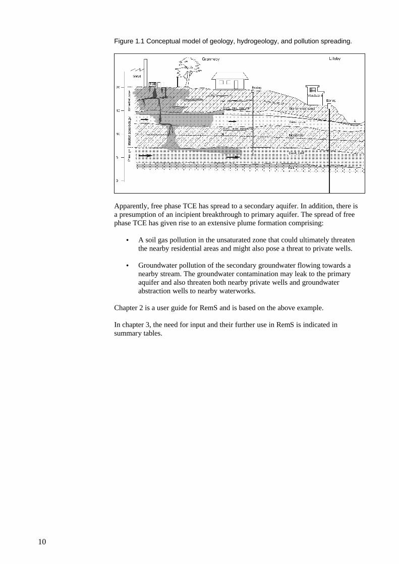
Studies have shown that surface spills and leaks from storage of Trichloroethylene (TCE) at Greenvillage Metal Works have resulted in a widespread contamination of soil and groundwater, as shown in Figure 1.1.
10
Figure 1.1 Conceptual model of geology, hydrogeology, and pollution spreading.
Apparently, free phase TCE has spread to a secondary aquifer. In addition, there is a presumption of an incipient breakthrough to primary aquifer. The spread of free phase TCE has given rise to an extensive plume formation comprising:
• A soil gas pollution in the unsaturated zone that could ultimately threaten the nearby residential areas and might also pose a threat to private wells.
• Groundwater pollution of the secondary groundwater flowing towards a nearby stream. The groundwater contamination may leak to the primary aquifer and also threaten both nearby private wells and groundwater abstraction wells to nearby waterworks.
Chapter 2 is a user guide for RemS and is based on the above example.
In chapter 3, the need for input and their further use in RemS is indicated in summary tables.
11
2 User Guide
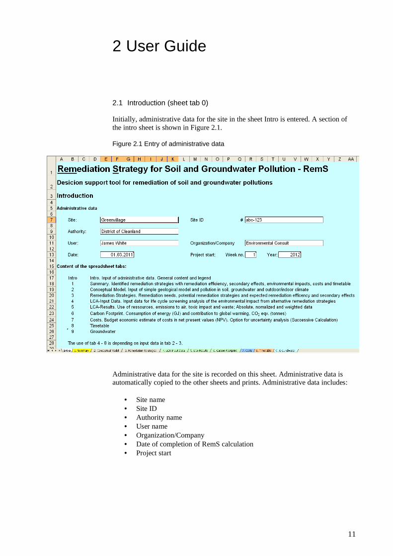
2.1 Introduction (sheet tab 0)
Initially, administrative data for the site in the sheet Intro is entered. A section of the intro sheet is shown in Figure 2.1.
Figure 2.1 Entry of administrative data
Administrative data for the site is recorded on this sheet. Administrative data is automatically copied to the other sheets and prints. Administrative data includes:
• Site name• Site ID• Authority name• User name• Organization/Company• Date of completion of RemS calculation• Project start
12
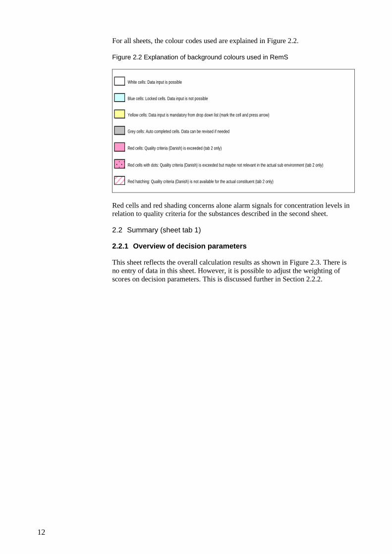
For all sheets, the colour codes used are explained in Figure 2.2.
Figure 2.2 Explanation of background colours used in RemS
White cells: Data input is possible
Blue cells: Locked cells. Data input is not possible
Yellow cells: Data input is mandatory from drop down list (mark the cell and press arrow)
Grey cells: Auto completed cells. Data can be revised if needed
Red cells: Quality criteria (Danish) is exceeded (tab 2 only)
Red cells with dots: Quality criteria (Danish) is exceeded but maybe not relevant in the actual sub environment (tab 2 only)
Red hatching: Quality criteria (Danish) is not available for the actual constituent (tab 2 only)
Red cells and red shading concerns alone alarm signals for concentration levels in relation to quality criteria for the substances described in the second sheet.
2.2 Summary (sheet tab 1)
2.2.1 Overview of decision parameters
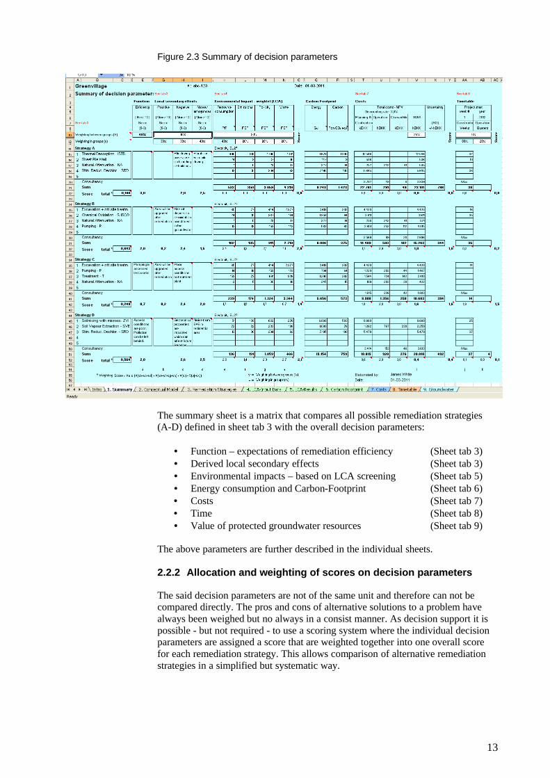
This sheet reflects the overall calculation results as shown in Figure 2.3. There is no entry of data in this sheet. However, it is possible to adjust the weighting of scores on decision parameters. This is discussed further in Section 2.2.2.
13
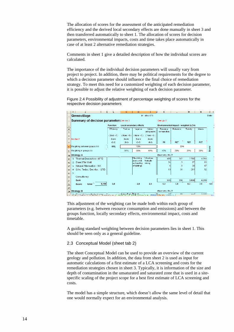
Figure 2.3 Summary of decision parameters
The summary sheet is a matrix that compares all possible remediation strategies (A-D) defined in sheet tab 3 with the overall decision parameters:
• Function – expectations of remediation efficiency (Sheet tab 3)• Derived local secondary effects (Sheet tab 3)• Environmental impacts – based on LCA screening (Sheet tab 5)• Energy consumption and Carbon-Footprint (Sheet tab 6)• Costs (Sheet tab 7)• Time (Sheet tab 8)• Value of protected groundwater resources (Sheet tab 9)
The above parameters are further described in the individual sheets.
2.2.2 Allocation and weighting of scores on decision parameters
The said decision parameters are not of the same unit and therefore can not be compared directly. The pros and cons of alternative solutions to a problem have always been weighed but no always in a consist manner. As decision support it ispossible - but not required - to use a scoring system where the individual decision parameters are assigned a score that are weighted together into one overall score for each remediation strategy. This allows comparison of alternative remediation strategies in a simplified but systematic way.
14
The allocation of scores for the assessment of the anticipated remediation efficiency and the derived local secondary effects are done manually in sheet 3 and then transferred automatically to sheet 1. The allocation of scores for decision parameters, environmental impacts, costs and time takes place automatically in case of at least 2 alternative remediation strategies.
Comments in sheet 1 give a detailed description of how the individual scores are calculated.
The importance of the individual decision parameters will usually vary from project to project. In addition, there may be political requirements for the degree to which a decision parameter should influence the final choice of remediation strategy. To meet this need for a customized weighting of each decision parameter, it is possible to adjust the relative weighting of each decision parameter.
Figure 2.4 Possibility of adjustment of percentage weighting of scores for the respective decision parameters
This adjustment of the weighting can be made both within each group of parameters (e.g. between resource consumption and emissions) and between the groups function, locally secondary effects, environmental impact, costs and timetable.
A guiding standard weighting between decision parameters lies in sheet 1. This should be seen only as a general guideline.
2.3 Conceptual Model (sheet tab 2)
The sheet Conceptual Model can be used to provide an overview of the current geology and pollution. In addition, the data from sheet 2 is used as input for automatic calculations of a first estimate of a LCA screening and costs for the remediation strategies chosen in sheet 3. Typically, it is information of the size and depth of contamination in the unsaturated and saturated zone that is used in a site-specific scaling of the project scope for a best first estimate of LCA screening and costs.
The model has a simple structure, which doesn’t allow the same level of detail that one would normally expect for an environmental analysis.
15
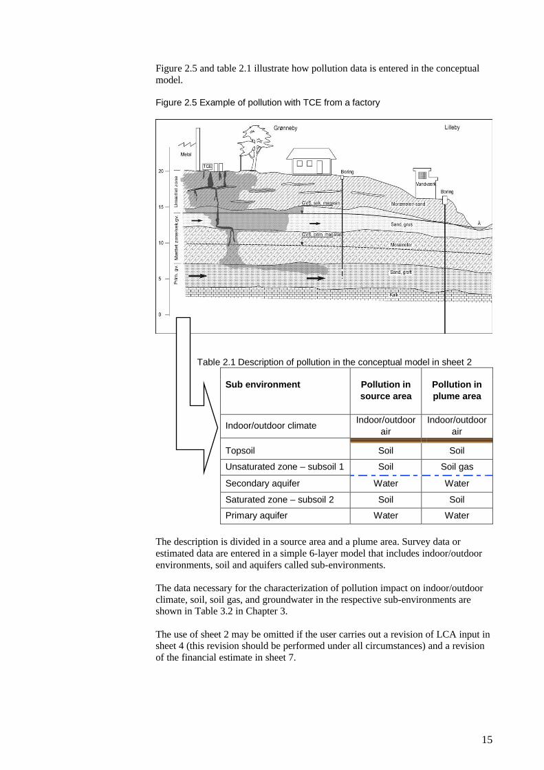
Figure 2.5 and table 2.1 illustrate how pollution data is entered in the conceptual model.
Figure 2.5 Example of pollution with TCE from a factory
Table 2.1 Description of pollution in the conceptual model in sheet 2
Sub environment Pollution in
source area
Pollution in
plume area
Indoor/outdoor climateIndoor/outdoor
air
Indoor/outdoor
air
Topsoil Soil Soil
Unsaturated zone – subsoil 1 Soil Soil gas
Secondary aquifer Water Water
Saturated zone – subsoil 2 Soil Soil
Primary aquifer Water Water
The description is divided in a source area and a plume area. Survey data or estimated data are entered in a simple 6-layer model that includes indoor/outdoor environments, soil and aquifers called sub-environments.
The data necessary for the characterization of pollution impact on indoor/outdoor climate, soil, soil gas, and groundwater in the respective sub-environments are shown in Table 3.2 in Chapter 3.
The use of sheet 2 may be omitted if the user carries out a revision of LCA input in sheet 4 (this revision should be performed under all circumstances) and a revision of the financial estimate in sheet 7.
16
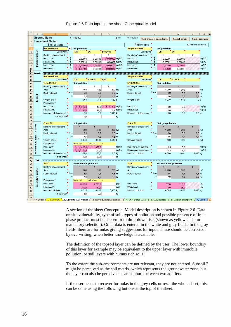
Figure 2.6 Data input in the sheet Conceptual Model
A section of the sheet Conceptual Model description is shown in Figure 2.6. Data on site vulnerability, type of soil, types of pollution and possible presence of free phase product must be chosen from drop-down lists (shown as yellow cells for mandatory selection). Other data is entered in the white and gray fields. In the gray fields, there are formulas giving suggestions for input. These should be corrected by overwriting, when better knowledge is available.
The definition of the topsoil layer can be defined by the user. The lower boundary of this layer for example may be equivalent to the upper layer with immobile pollution, or soil layers with humus rich soils.
To the extent the sub-environments are not relevant, they are not entered. Subsoil 2 might be perceived as the soil matrix, which represents the groundwater zone, but the layer can also be perceived as an aquitard between two aquifers.
If the user needs to recover formulas in the grey cells or reset the whole sheet, this can be done using the following buttons at the top of the sheet:
17
• ”Reset formulas in selected range”: Recovers formulas in marked cells”• ”Reset all formulas”: Recovers formulas in all grey cells, but all other data
are retained• ”Reset default values”: Recovers all formulas and deletes all entries in
sheet 2
For mobile contaminants, the source area shall be perceived as areas where seepage of dissolved and free phase contamination can occur. The plume area includes the part of the pollution that is spread as soil gas pollution in the unsaturated zone and as a groundwater contamination with dissolved substances.
Non / low mobile pollutions - such as heavy metals and tar substances - can occur in combination with mobile pollution and may be entered in both source and plume area. In the entry of affected areas there need not be a physical combination of contaminants in the same area.
In the description of pollution, the user shall for each sub-environment designate which of the listed pollutions that will determine the extent of potential remedial actions. Contaminations with "Priority 1" will be included in the further automated estimates on LCA screenings and costs of the selected remediation strategies.
18
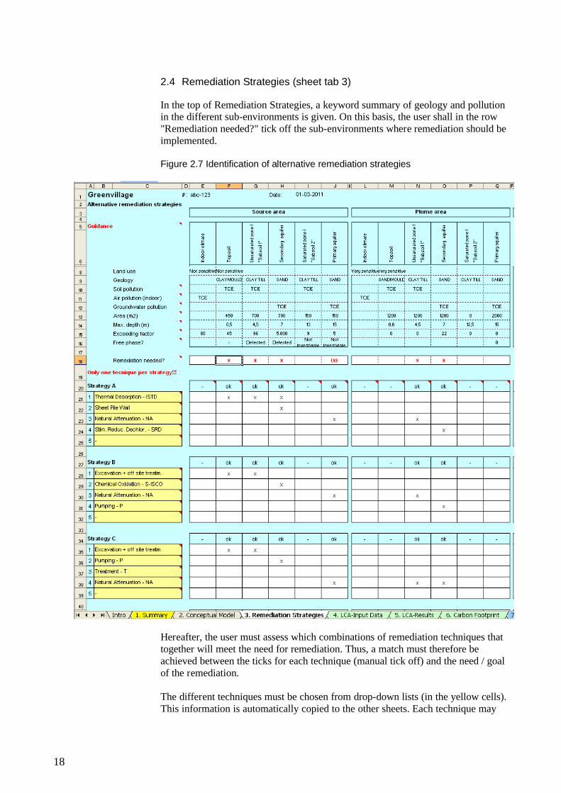
2.4 Remediation Strategies (sheet tab 3)
In the top of Remediation Strategies, a keyword summary of geology and pollution in the different sub-environments is given. On this basis, the user shall in the row "Remediation needed?" tick off the sub-environments where remediation should be implemented.
Figure 2.7 Identification of alternative remediation strategies
Hereafter, the user must assess which combinations of remediation techniques that together will meet the need for remediation. Thus, a match must therefore be achieved between the ticks for each technique (manual tick off) and the need / goal of the remediation.
The different techniques must be chosen from drop-down lists (in the yellow cells). This information is automatically copied to the other sheets. Each technique may
19
be chosen only once per strategy, otherwise there will arise conflict in calculating consumption, costs, etc.
Techniques available in RemS include:
1. Excavation/augering with off site biological treatment 2. Sheet Pile Wall 3. Pumping – P4. Soil Vapour Extraction – SVE5. Dual-Phase Extraction – DPE6. Surfactant-enhanced In Situ Chemical Oxidation – S-ISCO7. Stimulated Reductive Dechlorination – SRD8. Treatment – T (water and air)9. Soil mixing with Zero Valent Iron – ZVI 10. Natural Attenuation – NA11. Passive Soil Vapour Extraction – PSVE12. In Situ Thermal Desorption - ISTD (conductive heating)13. Steam Enhanced Extraction - SEE14. Electrical Resistivity Heating – ERH
Last in the drop-down list there is a "technique" called "specific consumption", which implies the possibility of direct input of energy consumption (electricity and diesel for entrepreneurial machines) and material consumption (such as concrete, asphalt, PVC, PE, steel, stainless steel, activated carbon , bentonite, and sand / gravel).
This enables addition of additional consumption that is not included in the standard techniques. This could be large dimension augered wells filled with concrete to ensure stability of an excavation, an access road with gravel, laying of asphalt or other. Each user must determine the expected consumption in absolute quantities, for example m3 concrete.
Excavation includes external biological soil remediation of contamination with lighter oil products. Other pollutants can with good approximation be simulated with this technique. It is noted that LCA calculations include that half of the amount of soil disposed of to a soil treatment plant are subsequently deposited. This contributes to the volume of bulk waste. The remainder is assumed reused, thus not contributing to environmental effects.
Chemical oxidation includes the opportunity to use sodium persulphate as oxidant in combination with sodium hydroxide for activating or potassium permanganate as oxidant. VeruSol can be included as surfactant.
Stimulated reductive dechlorination includes the possibility of using soya bean emulsion (EOS) or sodium formate (chemically similar to sodium lactate) as a substrate. As the bacterial culture KB1 is used.
Treatment can be combined to other techniques and include use of an LNAPL/DNAPL separator, stripping of water with an INKA ventilation or by filtration of water or air through activated carbon.
20
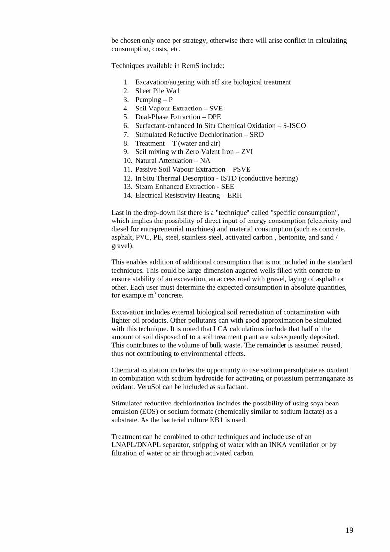
2.4.1 Assessment of remediation efficiency and secondary effects
In the right side of the sheet Remediation Strategies, cf. Figure 2.8, the user must give an assessment of the function of each remediation strategy (expectation of remediation efficiency and likelihood for effect) and derived secondary effects, including neighbours annoyances.
Figure 2.8 Assessment of remediation efficiency and derived secondary effects
This assessment is using a relative scoring system, where the most favourable outcome is given the value 3 and the worst outcome value 0. A guide for determining the scores is shown in comments in the header above the input data fields.
Any important remarks for the decision making process can be entered as a short comment which is transferred to the Summary sheet (sheet tab 1).
21
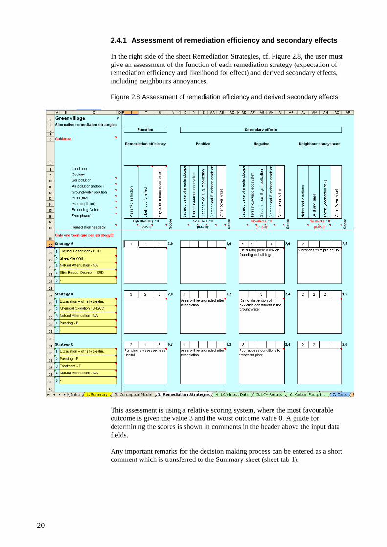
2.5 LCA- Input Data (sheet tab 4)
Appendix 1 sets out details of the LCA screening method.
LCA input includes input tables for life cycle screening of the selected remediation strategies. An example of an input data table is shown in Figure 2.9. Input tables are automatically created for the remediation techniques chosen by the user in sheet 3. The input tables show the main key-parameters for an overall description of the scope of the remediation project.
Figure 2.9 Correction of LCA input
On basis of the displayed key input, a set of data for unit energy and unit material consumption is generated forming the background for the LCA screening calculations for each technique. This data set is not visible to the user, but technique datasheets in Appendix 2 describe which activities are included in the LCA screening and which unit processes are used in each screening.
22
The applied unit processes that convert the unit energy consumption and consumption of unit materials to potential environmental impacts are documented in Appendix 3.
For each remediation technique, there is in the column "Standard" that display a data set for a "common scale project". In the example in Figure 2.9 a standard ISTD remediation based on heating of an area of 500 m2 to a depth of 7 m. Based on the user's description of the current geology and distribution of contamination in sheet 2, the input data for LCA screening is automatically corrected in the column "Auto adjusted", which is thus related to the site-specific conditions. In the next column "User adjusted " (not write protected), the user should correct the input if the user has a specific knowledge or expectation of a better estimate on the input data.
In the last column, the nominal values is automatically set, which are finally forming the basis for the LCA screening. A review from the user is needed to ensure that the auto-corrected data are approximate values to real situation. Highly divergent data can occur if the current geological conditions are not easily fittedinto the conceptual model in sheet 2, or if the user has chosen not to complete sheet 2.
Note that the corrected values chosen by the user in sheet 3 is reset when one technique is replaced with another.
In Appendix 5, forms for data collection for the LCA screening calculation are attached.
2.6 LCA results (sheet tab 5)
2.6.1 Screening parameters
RemS will automatically perform a life cycle screening, which as the result gives the environmental impact of the remediation strategy. The calculation is based on the input tables, section 2.5.
The environmental impact is expressed as an inventory of the consumption of resources that includes:
• Energy resources• Metals• Sand and gravel
And the impact potential for:
• Emissions to the atmosphere• Human and environmental toxic effects• Generation of waste
23
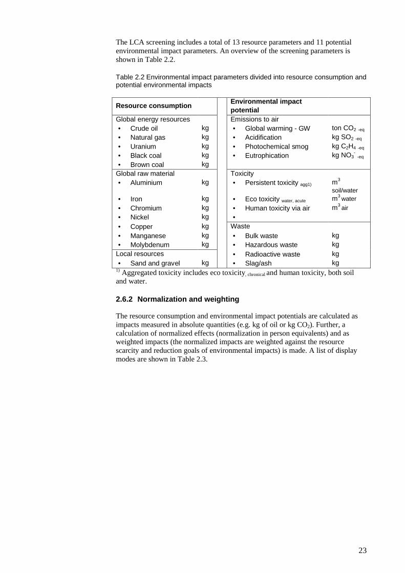
The LCA screening includes a total of 13 resource parameters and 11 potential environmental impact parameters. An overview of the screening parameters is shown in Table 2.2.
Table 2.2 Environmental impact parameters divided into resource consumption and potential environmental impacts
Resource consumptionEnvironmental impact
potential
Global energy resources Emissions to air
• Crude oil kg • Global warming - GW ton CO2 -eq
• Natural gas kg • Acidification kg SO2 -eq
• Uranium kg • Photochemical smog kg C2H4 -eq
• Black coal kg • Eutrophication kg NO3-
-eq
• Brown coal kg
Global raw material Toxicity
• Aluminium kg • Persistent toxicity agg1) m3
soil/water
• Iron kg • Eco toxicity water, acute m3 water
• Chromium kg • Human toxicity via air m3 air
• Nickel kg •
• Copper kg Waste
• Manganese kg • Bulk waste kg
• Molybdenum kg • Hazardous waste kg
Local resources • Radioactive waste kg
• Sand and gravel kg • Slag/ash kg1) Aggregated toxicity includes eco toxicity, chronical and human toxicity, both soil and water.
2.6.2 Normalization and weighting
The resource consumption and environmental impact potentials are calculated as impacts measured in absolute quantities (e.g. kg of oil or kg CO2). Further, a calculation of normalized effects (normalization in person equivalents) and as weighted impacts (the normalized impacts are weighted against the resource scarcity and reduction goals of environmental impacts) is made. A list of display modes are shown in Table 2.3.
24
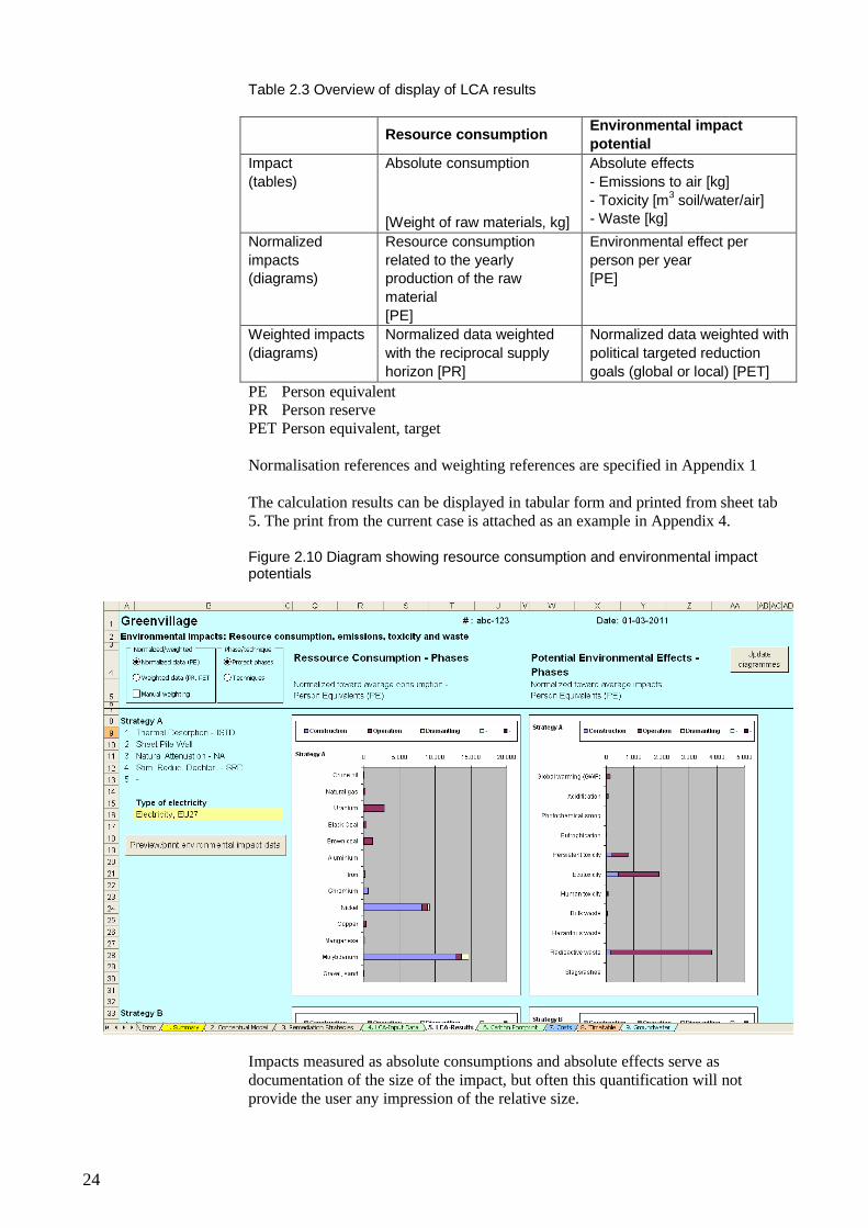
Table 2.3 Overview of display of LCA results
Resource consumptionEnvironmental impact
potential
Impact
(tables)
Absolute consumption
[Weight of raw materials, kg]
Absolute effects
- Emissions to air [kg]
- Toxicity [m3 soil/water/air]- Waste [kg]
Normalized
impacts(diagrams)
Resource consumption
related to the yearly production of the raw
material
[PE]
Environmental effect per
person per year[PE]
Weighted impacts
(diagrams)
Normalized data weighted
with the reciprocal supply
horizon [PR]
Normalized data weighted with
political targeted reduction
goals (global or local) [PET]
PE Person equivalentPR Person reservePET Person equivalent, target
Normalisation references and weighting references are specified in Appendix 1
The calculation results can be displayed in tabular form and printed from sheet tab 5. The print from the current case is attached as an example in Appendix 4.
Figure 2.10 Diagram showing resource consumption and environmental impact potentials
Impacts measured as absolute consumptions and absolute effects serve as documentation of the size of the impact, but often this quantification will not provide the user any impression of the relative size.

25
The normalized view gives a relative size of the project's impacts. The project’s impacts are compared with the average annual impact from an average person's annual loads, whereby the unit becomes person equivalent. This allows a quantification which immediately gives an impression of the environmental load sizes. Furthermore, the graphic display allows a visual comparison of alternative remediation strategies.
The normalization reference is "a world citizen" for global resources and global warming and "an EU citizen" for the other environmental impacts except for waste production, since there are no EU normalization references for waste. For waste generation is instead used a normalization reference based on the Danish / Swedish conditions.
Weighted impacts in principle allows for an assessment of the severity of resource consumption and environmental impacts.
Consumption of resources is shown with a weighting factor which is the reciprocal value of the supply horizon of the economically accessible reserves of that resource. Environmental impacts appear with a weighting factor corresponding to the reduction goal for the actual discharge that is determined on the basis of international agreements.
In addition, sheet 5 allows for a customized weighting that can be composed of two contributions. If an organization has chosen a set of weighting factors, these may be entered as a local political weighting. If there are particular site-specific terms –e.g. a densely populated residential area - it is possible to perform a manual weighting of e.g. toxic effects.
Results are shown as bars that can be chosen to be divided into project phases (planning and construction, operation, and dismantling) or divided into the individual techniques that are part of that strategy.
When choosing a phase / technology, the graphs are updated in the same scale, whereby the graphic profile of the strategies will be directly comparable.
For remediation strategies involving a significant consumption of electricity, the choice of the type of electricity may be significant. In sheet 5, there is a selection field for type of electricity for each strategy. This allows an immediate view of the consequences of the choice of electricity. By creating two similar remediation strategies, the importance of such marginal types of electricity versus conventional electricity can be compared.
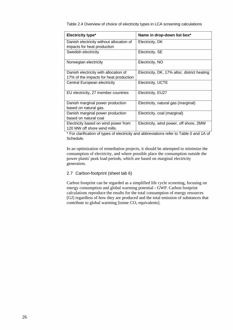
The types of electricity available in RemS are shown in Table 2.4. The selected type of electricity is displayed on sheet 1 Summary and sheet 6 Carbon footprint.
26
Table 2.4 Overview of choice of electricity types in LCA screening calculations
Electricity type* Name in drop-down list box*
Danish electricity without allocation of impacts for heat production
Electricity, DK
Swedish electricity Electricity, SE
Norwegian electricity Electricity, NO
Danish electricity with allocation of 17% of the impacts for heat production
Electricity, DK, 17% alloc. district heating
Central European electricity Electricity, UCTE
EU electricity, 27 member countries Electricity, EU27
Danish marginal power production based on natural gas.
Electricity, natural gas (marginal)
Danish marginal power production
based on natural coal
Electricity, coal (marginal)
Electricity based on wind power from
120 MW off shore wind mills.
Electricity, wind power, off shore, 2MW
* For clarification of types of electricity and abbreviations refer to Table 0 and 1A of Schedule.
In an optimization of remediation projects, it should be attempted to minimize the consumption of electricity, and where possible place the consumption outside the power plants' peak load periods, which are based on marginal electricity generation.
2.7 Carbon-footprint (sheet tab 6)
Carbon footprint can be regarded as a simplified life cycle screening, focusing on energy consumption and global warming potential - GWP. Carbon footprint calculations reproduce the results for the total consumption of energy resources [GJ] regardless of how they are produced and the total emission of substances that contribute to global warming [tonne CO2 equivalents].
27
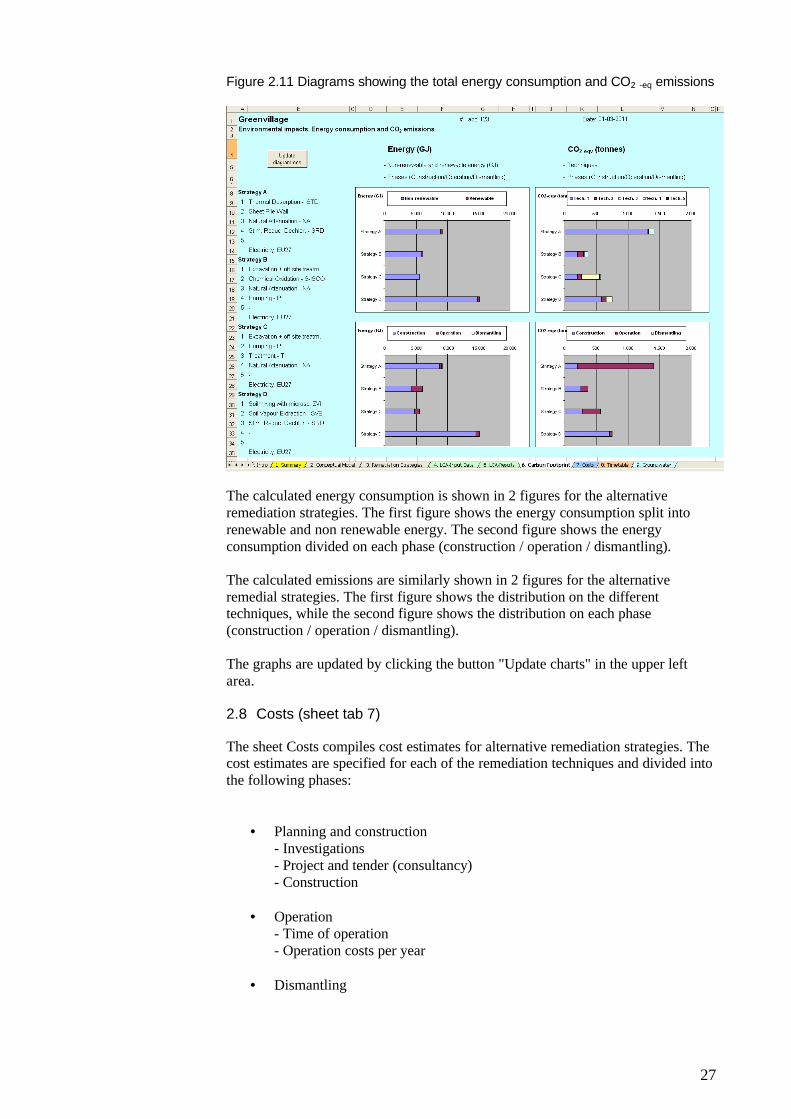
Figure 2.11 Diagrams showing the total energy consumption and CO2 -eq emissions
The calculated energy consumption is shown in 2 figures for the alternative remediation strategies. The first figure shows the energy consumption split into renewable and non renewable energy. The second figure shows the energy consumption divided on each phase (construction / operation / dismantling).
The calculated emissions are similarly shown in 2 figures for the alternative remedial strategies. The first figure shows the distribution on the different techniques, while the second figure shows the distribution on each phase (construction / operation / dismantling).
The graphs are updated by clicking the button "Update charts" in the upper left area.
2.8 Costs (sheet tab 7)
The sheet Costs compiles cost estimates for alternative remediation strategies. The cost estimates are specified for each of the remediation techniques and divided into the following phases:
• Planning and construction- Investigations- Project and tender (consultancy)- Construction
• Operation- Time of operation- Operation costs per year
• Dismantling
28
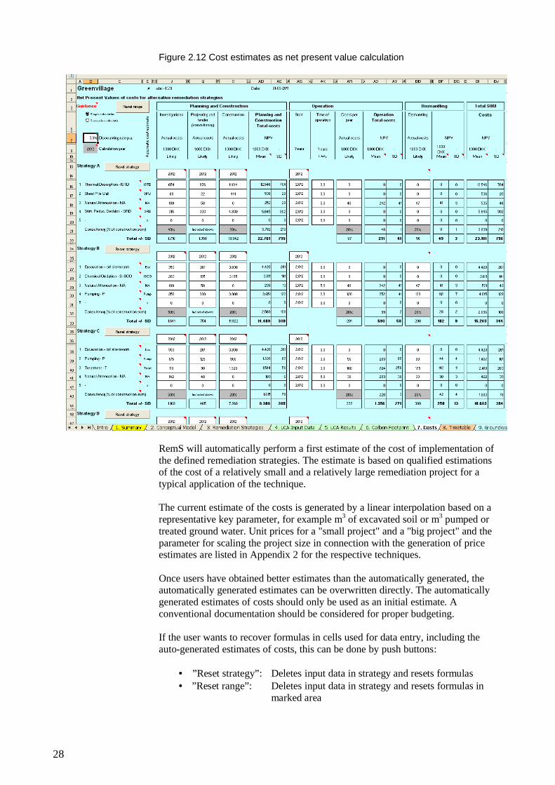
Figure 2.12 Cost estimates as net present value calculation
RemS will automatically perform a first estimate of the cost of implementation of the defined remediation strategies. The estimate is based on qualified estimations of the cost of a relatively small and a relatively large remediation project for a typical application of the technique.
The current estimate of the costs is generated by a linear interpolation based on a representative key parameter, for example m3 of excavated soil or m3 pumped or treated ground water. Unit prices for a "small project" and a "big project" and the parameter for scaling the project size in connection with the generation of priceestimates are listed in Appendix 2 for the respective techniques.
Once users have obtained better estimates than the automatically generated, the automatically generated estimates can be overwritten directly. The automatically generated estimates of costs should only be used as an initial estimate. Aconventional documentation should be considered for proper budgeting.
If the user wants to recover formulas in cells used for data entry, including the auto-generated estimates of costs, this can be done by push buttons:
• ”Reset strategy”: Deletes input data in strategy and resets formulas• ”Reset range”: Deletes input data in strategy and resets formulas in
marked area
29
A marked area may be one single cell, an area of more cells or the entire sheet.
It is noted that the pricing of the individual techniques generally relates to entrepreneurial and construction costs, including costs for laboratory analysis. Consulting is priced as a percentage of the entrepreneurial and construction costs. The reason is that consultancy costs are often not specified on the individual techniques, but settled for the overall strategy. The users may choose to change the percentage surcharge for consultancy or set the percentage at 0% and include the consultancy costs in the specific techniques. For projecting and tender it is merely a consultancy cost to be specified for each remediation technique.
2.8.1 Net Present Value calculation
The cost estimate includes a net present value (NPV) calculation of future costs /1/. This allows a comparison of alternative projects with different payment schedules.
In the calculation of the net present value, a discount rate is used. In the context of socio-economic assessments of environmental projects is recommended to use 3.0% as interest rate /2/. Interest rates can be modified by the user at the top left of the sheet whereby sensitivity analysis for different rates can be easily implemented. For sensitivity calculations, discount rates of 1 and 5% are recommended.
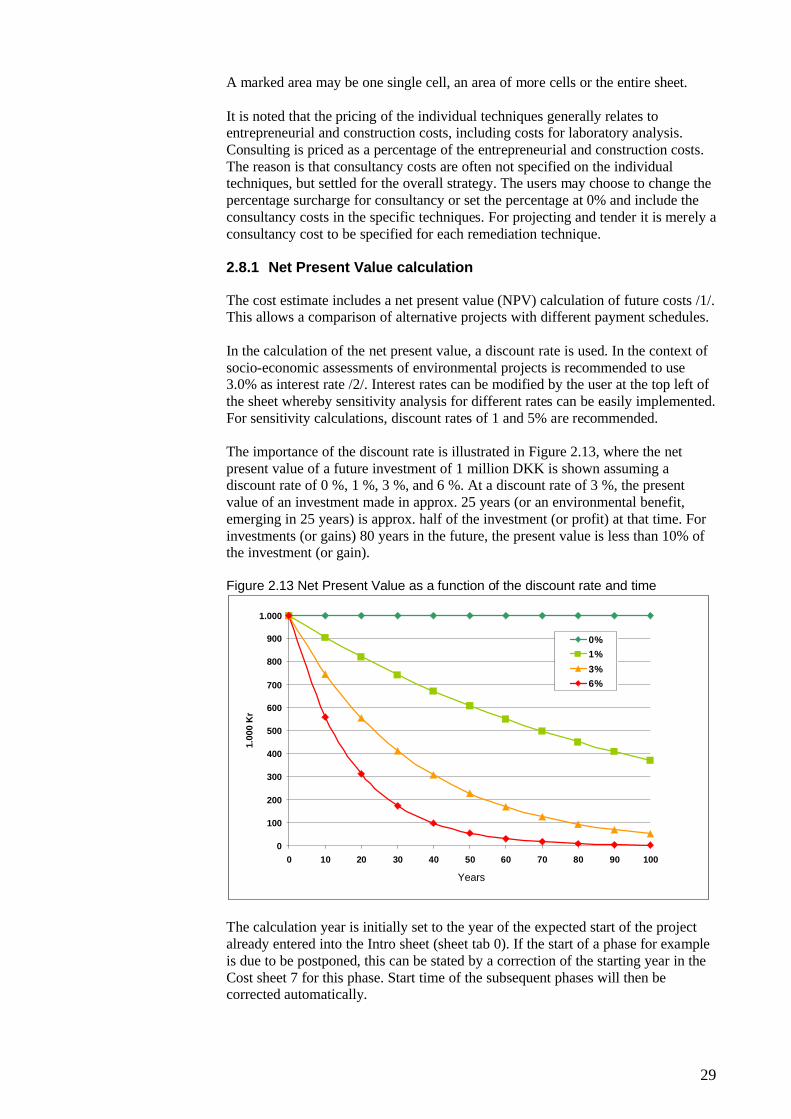
The importance of the discount rate is illustrated in Figure 2.13, where the net present value of a future investment of 1 million DKK is shown assuming a discount rate of 0 %, 1 %, 3 %, and 6 %. At a discount rate of 3 %, the present value of an investment made in approx. 25 years (or an environmental benefit, emerging in 25 years) is approx. half of the investment (or profit) at that time. For investments (or gains) 80 years in the future, the present value is less than 10% of the investment (or gain).
Figure 2.13 Net Present Value as a function of the discount rate and time
0
100
200
300
400
500
600
700
800
900
1.000
0 10 20 30 40 50 60 70 80 90 100
År
1.0
00 K
r
0%
1%
3%
6%
The calculation year is initially set to the year of the expected start of the project already entered into the Intro sheet (sheet tab 0). If the start of a phase for example is due to be postponed, this can be stated by a correction of the starting year in the Cost sheet 7 for this phase. Start time of the subsequent phases will then be corrected automatically.
Years
30
Where "treatment trains" are included, this can be simulated by adjusting appropriate start time for each technique in sheet 7.
2.8.2 Successive Calculation
Cost estimates for each of the alternative remediation strategies are in principle based on a simple calculation, where cost estimates are based on the "most likely" unit price, volume, and duration of operation.
However, there is often a great uncertainty in estimates of price and time. Successive Calculation is an accepted method based on Bayesian statistics, where it is assumed that the difference between a subjectively estimated value and the true value can be treated as a random variable.
In estimates of price or time, you can make a subjective assessment of the value as:
• Minimum• Likely• Maximum
If the assessments of minimum and maximum values are assumed to be within a 98% confidence interval, the approximate value of mean, variance and standard deviation can be calculated as follows /3/:
Mean value ~5
MaxLikely*3Min ++
Variance ~
2
5
− MinMax
Standard deviation = Variance
With an option button at the top left of Cost sheet is it possible to extend the estimate with a Successive Calculation, since input on costs and operating time are extended to include the expected minimum and maximum values.
31
Figure 2.14 Cost estimates based on Successive Calculation
A calculation of a mean and a standard deviation on on the individual items is hereby performed, allowing the major uncertainties to be identified, and thus making it possible to successively pursue and reduce the principal uncertainties in detail estimates where necessary. This could help avoid unnecessary detailing in calculations, where the uncertainty is of secondary importance.
Minimum and maximum values should be set conservatively. This will generate a distribution on each of the remediation techniques and disclose the greatest uncertainties.
The estimated costs are shown as a mean value with a standard deviation value onthe individual items. A large spread is obviously due to a great uncertainty. This allows you to successively refine the cost estimates, where the uncertainty is to high.
It is noted that standard deviation values on individual items can not be readily summed. The standard deviation on main items is based on the calculation of the variance on the main item concerned.
32
2.9 Timetable (sheet tab 8)
The remedial strategies selected are automatically transferred to the Timetable sheet from sheet 3.
Figure 2.15 Timetable input
The timetable is initially scaled on either weekly or monthly basis. Under the timetable for the planning and construction phase, is a timetable for eventual operation phase. Similarly, for operating periods of each strategy, monthly or quarterly view can be chosen.
For each technique, the end of entry is marked with an "s". There must be no other kind of marking of end of activities in the schedule. For techniques with a subsequent operating period, this is marked to the far right with a tick.
Subsequently, the expected completion of the operation period is also marked with an "s". Completion of the last activity is marked with an "s" in the cell immediately after the last activity. The marking "s" is used to calculate the duration of the project in the Summary sheet (sheet tab 1) and therefore necessary if the timetable is included in the final assessment.
2.10 Value of groundwater protection (sheet tab 9)
Remediation of polluted sites is often carried out with the purpose of protecting thegroundwater. Therefore it would be appropriate to quantify the environmental benefits of either remediation or protection of the groundwater. It is stressed that the value of groundwater protection is conditional on the groundwater resource is not threatened by other sources of pollution. If several sites threaten the same groundwater resource, this must be taken into account in the decision process.
Sheet 9 Groundwater allows a quantification of environmental benefits from an estimate of how large the protected groundwater resource is (m3) and a nominalunit price (DKK/m3) of the protected groundwater.
33
Figure 2.16 Capitalization of the value of groundwater protection
2.10.1 The groundwater resource
Initially, input information is given on whether the groundwater resource is part of a groundwater protection area, on the quantity of abstracted groundwater in the area, and the type of aquifer (secondary or primary aquifer). This information is only for informal purpose and is not used in further calculations.
2.10.2 Threat to groundwater
Risk of groundwater pollution from actual siteSubsequently, it is indicated to which extent the contamination on the actual siteposes a threat to groundwater resources. This information is given as a percentage that should be estimated according to the risk assessment of the groundwater threat.
34
Figure 2.17 Examples of expected groundwater threat without implementation of remediation
Figure 2.17 shows 2 examples of an expected development in the pollution impact on an aquifer, if no remedial action is taken. Scenario A illustrates a location where there is an assessed risk of a low pollution impact on the ground water, almostequivalent to the accept criteria. The assessment may be based on a risk assessment with a subsequent sensitivity analysis showing the uncertainty of the assessment. In RemS, the threat level should be expressed as ~50%. Scenario B illustrates a location with a high risk of a heavy pollution impact on the ground water. In RemS, the threat level should be set to 100%.
If the ground water is already affected by pollution above the accept criteria, enter100%.
Volume of protected groundwaterThen the amount of groundwater that is expected to be protected is estimated. The user must choose whether the protected groundwater quantity shall be accounted as an annually groundwater flux (m3/year) or a total volume (m3). Here should be argued for the choice of calculation method on the basis of site-specific conditions.
The groundwater flux can for example be estimated as the amount of ground water that is assessed to be affected above the accept criteria when passing the area in which seepage of pollution may occur. If the site is located in a catchment area, a groundwater flux equivalent to the annual abstraction may be chosen.
The total groundwater volume may for example be estimated on the basis of an assessment / modelling of the maximum spatial distribution of a pollution plumetaking dispersion and degradation conditions into consideration.
It is possible by Successive Calculation to quantify the uncertainty in the estimate of the quantity of the protected groundwater. The user can thus indicate an estimated minimum quantity, a likely quantity, and a maximum quantity by which a mean value and a standard deviation of the protected groundwater quantity is generated. The calculation principle is reviewed in section 2.8.2.
If an actual uncertainty assessment is not requested, only an estimate of the likely protected groundwater quantity is given.
35
2.10.3 Valuing
Unit value for protected groundwaterAs mentioned initially, the valuation is based on a unit value (kr/m3) for the protected groundwater.
This unit value is determining for the value of groundwater protection and at the same time difficult to estimate accurately. In principle, one can estimate the unit price based on a valuation study, which may contain several components:
• Use value, provided groundwater catchment takes place• Option value of a potential future groundwater catchment• Existence value for humans and environment
The use value and the option value can be assessed by estimates of either the cost for an alternative water supply or water treatment of groundwater at the waterworks (whether this is politically acceptable or not). The existence value is ethically contingent and can not be precisely determined, since the value of clean ground water as a resource for humans and the environment now and in future is a matter of perception by individuals.
There is no recommended unit value for protected / recovered groundwater, but one can easily make alternative calculation scenarios. The estimated cost for an alternative water supply could here be a minimum scenario.
Discount rateIn the net present value calculation of the future environmental benefit there is used the same back discount rate as the interest rate in the cost estimate. The discount rate is automatically transferred from sheet 7 to sheet 9.
It is possible to immediately carry out a sensitivity rating, in that the user may enter an alternative rate. The calculation result for the alternative rate will be displayed immediately. The alternative rate is reset automatically when the worksheet is closed. Therefore, calculation results with an alternative rate can not be saved.
Time aspectsDiscounting implies that the value of groundwater protection decreases the longer it takes before the desired effect is achieved.
The user must assess how many years it will take from the start of remediation to the targeted effect on the ground water is achieved (accept criteria). This could be the number of years until the groundwater threshold values is expected to be met.
In the net present value calculation, this corresponds to the time when the environmental benefits of remediation are achieved. The total time is the period from calculation date until start of remediation plus the period until the targeted effect of the preventing measures is achieved.
The time of calculation (year) is defined on sheet 0 Intro and automatically repeated on sheet 9.
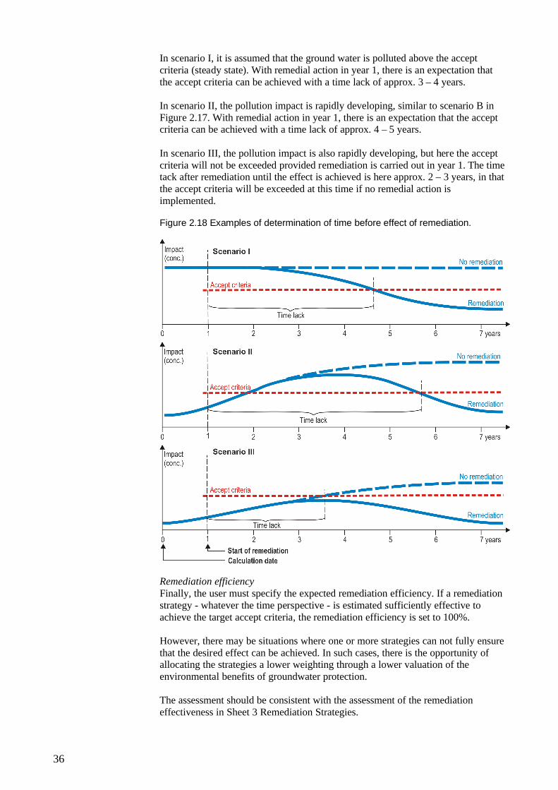
The time after remediation is started and until the effect is achieved must be assessed by the user. As a guide for this assessment is in Figure 2.18 shown 3 scenarios (I - III), which all have year 0 as calculation date and year 1 as start of remediation.
36
In scenario I, it is assumed that the ground water is polluted above the accept criteria (steady state). With remedial action in year 1, there is an expectation that the accept criteria can be achieved with a time lack of approx. 3 – 4 years.
In scenario II, the pollution impact is rapidly developing, similar to scenario B in Figure 2.17. With remedial action in year 1, there is an expectation that the acceptcriteria can be achieved with a time lack of approx. 4 – 5 years.
In scenario III, the pollution impact is also rapidly developing, but here the acceptcriteria will not be exceeded provided remediation is carried out in year 1. The time tack after remediation until the effect is achieved is here approx. 2 – 3 years, in thatthe accept criteria will be exceeded at this time if no remedial action is implemented.
Figure 2.18 Examples of determination of time before effect of remediation.
Remediation efficiencyFinally, the user must specify the expected remediation efficiency. If a remediation strategy - whatever the time perspective - is estimated sufficiently effective to achieve the target accept criteria, the remediation efficiency is set to 100%.
However, there may be situations where one or more strategies can not fully ensure that the desired effect can be achieved. In such cases, there is the opportunity of allocating the strategies a lower weighting through a lower valuation of the environmental benefits of groundwater protection.
The assessment should be consistent with the assessment of the remediation effectiveness in Sheet 3 Remediation Strategies.
37
Calculation of net present value of protected groundwaterThe calculated environmental benefit only include the years after the remediation is expected to be effective.
If a flux calculation is selected, the value of the groundwater protection is calculated as the annual environmental benefit from the time the effect of a remediation effort is expected to be achieved. For example, a remediation can leadto a fulfilment of the requirement for the groundwater quality 5 years after the remediation. In this case, the environmental benefit is calculated as the net present value of the environmental benefit from year 5 and the yearly benefit in years thereafter (the calculation is limited to 1,000 years after the remediation).
If a total volume calculation is selected then the value of the groundwater protection is calculated as the net present value of environmental benefits obtained when the effect of the remediation effort is expected to be achieved. For example, a remediation can lead to a fulfilment of the requirement for the groundwater quality for the full volume of the affected groundwater body 5 years after the remediation. In this case, the environmental benefit is calculated as the net present value of the entire environmental benefit expected in year 5 after the remediation.
In the following is referred to index (a) – (d) in figure 2.16
The value of the protected groundwater resource V is calculated as a net present value (NPV) of the annual groundwater volume (b) that are protected (flux based calculation) weighted by the risk that the groundwater resources are threatened (a) and the expected remediation efficiency (d).
V = a * d * NPV(b)
The valuation of the groundwater protection is thus directly proportional to the percentages given for the site to represent an actual risk of pollution to the ground water (a) and the assessed remediation efficiency of the individual remediation strategies (d).
The standard deviation on the value of the protected groundwater resource VSD is linked only to the uncertainty of the size of the protected groundwater resource (c).
VSD = a * d * NPV(c)
If the valuation relates to a total groundwater volume, the calculation is made in the same way, using (e) as the mean value of the protected volume of water instead of (b) and the standard deviation (f) instead of (c) in the above formulas.
2.11 Hidden sheets
The following sheets are hidden:• Input data (technique specifique setup)• Unit processes• Normalizing and weighting• Lists• Calculation• Environmental impact• Reset_tab 2• Reset_tab 7

38
The hidden sheets contain references, working calculations, and LCA dataautomatically used in the displayed sheet.
Calculations in the whole excel sheet are primarily based on direct and indirect references with lookup functions. Therefore, names of remediation techniques can only be changed one place to avoid losing the reference.
For uniformity of the charts, however, VBA coding (macros) has been used.
39
3 Input data to RemS
In the following, an overview of the need of and application of input data is given.
3.1 Intro Sheet
Administrative data (reference), [unit] Application
Site name Copied to all sheets
Site ID Copied to all sheets
Authority name Documentation
User name [name/initials] Documentation
Organization/Company Documentation
Date of completion of RemS
calcaulation[day, month, year] Copied to all sheets
Project start [week, year]Present value calculation
and timetable
3.2 Conceptual Model
Input data (reference), [unit] Application
Excee
din
g o
f
qua
lity
crite
ria
Ma
ss c
alc
ula
tion
Co
st
estim
ate
LC
A s
cre
en
ing
Pollution constituents (choice from list) x x x x
Sensitivity for human exposure
(choice from list) x
Geology, soil type (choice from list) x
Area of pollutions [m2] x x
Depth interval [m] x x
Concentration, maximum [mg/m3, mg/kg, •g/l] x
Concentration, mean [mg/m3, mg/kg, •g/l] x
Free phase (source area) [kg] x x
Priority of pollution for
remediation design[-] x x
40
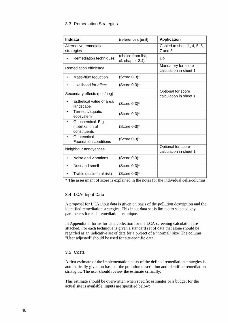
3.3 Remediation Strategies
Inddata (reference), [unit] Application
Alternative remediation
strategies
Copied to sheet 1, 4, 5, 6,
7 and 8
• Remediation techniques(choice from list,
cf. chapter 2.4)Do
Remediation efficiencyMandatory for score
calculation in sheet 1
• Mass-/flux reduction (Score 0-3)*
• Likelihood for effect (Score 0-3)*
Secondary effects (pos/neg)Optional for scorecalculation in sheet 1
• Esthetical value of area/
landscape(Score 0-3)*
• Terrestic/aquatic
ecosystem(Score 0-3)*
• Geochemical. E.g. mobilization of
constituents
(Score 0-3)*
• Geotecnical. Foundation conditions
(Score 0-3)*
Neighbour annoyancesOptional for score
calculation in sheet 1
• Noise and vibrations (Score 0-3)*
• Dust and smell (Score 0-3)*
• Traffic (accidental risk) (Score 0-3)*
* The assessment of score is explained in the notes for the individual cells/columns
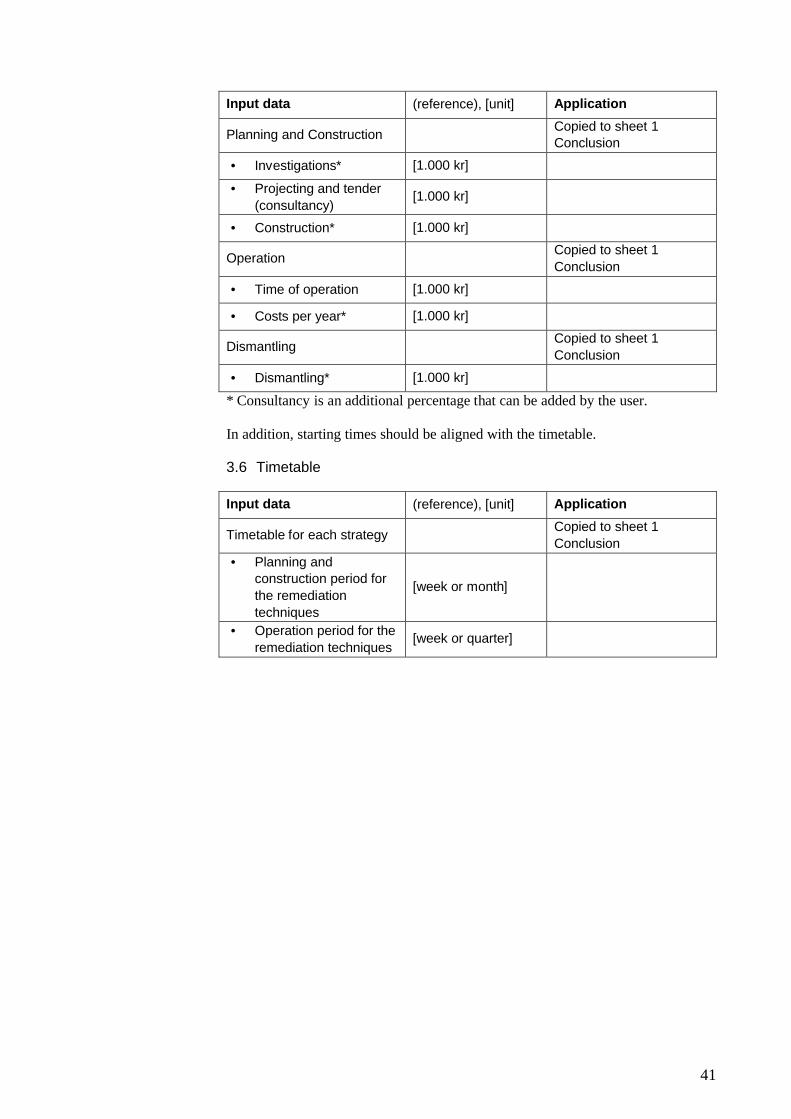
3.4 LCA- Input Data
A proposal for LCA input data is given on basis of the pollution description and theidentified remediation strategies. This input data set is limited to selected key parameters for each remediation technique.
In Appendix 5, forms for data collection for the LCA screening calculation are attached. For each technique is given a standard set of data that alone should be regarded as an indicative set of data for a project of a "normal" size. The column "User adjusted" should be used for site-specific data.
3.5 Costs
A first estimate of the implementation costs of the defined remediation strategies is automatically given on basis of the pollution description and identified remediationstrategies, The user should review the estimate critically.
This estimate should be overwritten when specific estimates or a budget for the actual site is available. Inputs are specified below:
41
Input data (reference), [unit] Application
Planning and ConstructionCopied to sheet 1 Conclusion
• Investigations* [1.000 kr]
• Projecting and tender
(consultancy)[1.000 kr]
• Construction* [1.000 kr]
OperationCopied to sheet 1
Conclusion
• Time of operation [1.000 kr]
• Costs per year* [1.000 kr]
DismantlingCopied to sheet 1
Conclusion
• Dismantling* [1.000 kr]
* Consultancy is an additional percentage that can be added by the user.
In addition, starting times should be aligned with the timetable.
3.6 Timetable
Input data (reference), [unit] Application
Timetable for each strategyCopied to sheet 1
Conclusion
• Planning and construction period for
the remediation
techniques
[week or month]
• Operation period for the
remediation techniques [week or quarter]

42
43
4 References
1. Lynggård, P.: "Investering og financiering". Handelshøjskolernes Forlag.2. Danmarks Miljøundersøgelser, Miljøstyrelsen og Skov- og Naturstyrelsen
(2000): ”Samfundsøkonomisk vurdering af miljøprojekter”.3. Lictenberg, S. (1974): "The Successive Principle", PMI-74, proc. 6-ann.
Seminar, Project Managament Institute, Washington DC, 1974 p. 570 - 78.4. Banestyrelsen rådgivning; HOH Vand og Miljø A/S; NIRAS Rådgivende
ingeniører og planlæggere A/S; Revisorsamvirket / Pannell Kerr Forster (2000): Miljørigtig oprensning af forurenede grunde. EU LIFE Project no. 96ENV/DK/0016. København, Danmark. Udarbejdet for Banestyrelsen, DSB og Miljøstyrelsen.
5. Bayer, P.; Heuer E.; Karl U.; Finkel M. (2005): Economical and ecological comparison of granular activated carbon (GAC) adsorber refill strategies. Water Research 2005, 39 (9), 1719-1728.
6. Energinet.dk (2008): Miljørapport 2008. Baggrundsrapport. Online udgave, April 2008.
7. Frischknecht, R.; Jungbluth N.; Althaus H.-J.; Doka G.; Dones R.; Heck T.; Hellweg S.; Hischier R.; Nemecek T.; Rebitzer G.; Spielmann M.; Wernet G. (2007): Overview and Methodology. ecoinvent report No. 1. 2007, Swiss Centre for Life Cycle Inventories, Dübendorf, 2007.
8. Hauge, O. (2009): Personal communication with O. Hauge, RGS90 A/S, Copenhagen, Denmark, via telephone 21-01-2009.

The Capital Region of DenmarkEnvironmental Department
RemSAppendices to User Guide
Remediation Strategy for Soil and Groundwater Pollution – RemS
Decision Support Tool
RemS is developed by NIRAS in collaboration with Gitte Lemming, DTU Environment, Technical University of Denmark.
Version 2.0. Marts 2011.

3
Appendices
1 PRINCIPLES FOR LIFE CYCLE ASSESSMENT 5
2 DATA SHEETS - TECHNIQUES 9
2.1 GENERAL INFORMATION ON LCA INPUT DATA 122.1.1 The investigation phase 132.1.2 Planning, construction, and operational phases 132.1.3 Control investigations 14
2.2 LCA INPUT DATA ON THE INDIVIDUAL TECHNIQUES 142.2.1 Excavation/augering with off site biological treatment 142.2.2 Sheet Pile Wall 162.2.3 Pumping – P 172.2.4 Soil Vapor Extraction – SVE 192.2.5 Dual-Phase Extraction – DPE 202.2.6 Surfactant-enhanced In Situ Chemical Oxidation – S-ISCO 212.2.7 Stimulated Reductive Dechlorination – SRD 232.2.8 Treatment – T (water and air) 252.2.9 Soil mixing with Zero Valent Iron – ZVI 272.2.10 Natural Attenuation – NA 282.2.11 Passive Soil Vapor Extraction – PSVE 292.2.12 In Situ Termal Desorption - ISTD (conductive heating) 302.2.13 Steam Enhanced Extraction – SEE 312.2.14 Electrical Resistivity Heating – ERH 332.2.15 Specific consumption 35
2.3 SPECIFIC ACTIVITIES 362.3.1 Transport 362.3.2 Boreholes/Wells 362.3.3 Entrepreneurial work 372.3.4 Other material consumption 37
2.4 UNIT PRICES 38
3 UNIT PROCESSES 43
4 ENVIRONMENTAL IMPACTS 55
5 DATA COLLECTION FOR LCA SCREENING CALCULATIONS 61

4

5
1 Principles for Life Cycle Assessment
The life cycle assessments translate the environmental exchanges from the inventory into environmental impacts using environmental assessment models (impact assessment models). The environmental assessment model used in RemS is the EDIP97 method (Wenzel et al. 1997), which contains the following impact categories:
Emissions:
• Global warming (ton CO2 eq)• Ozone depletion (kg CFC-11 eq)• Photochemical ozone formation (smog) (kg C2H4 eq)• Acidification (kg SO2 eq)• Eutrophication (NO3
- eq)
Toxic impacts:
• Human toxicity via air (m3 air)• Ecotoxicity, water, acute (m3 water)• Persistent toxicity§ Human toxicity via water (m3 water)§ Human toxicity via soil (m3 soil)§ Ecotoxicity, water, cronic (m3 water)§ Ecotoxicity, soil (m3 soil)
Waste:
• Bulk waste (kg)• Hazardous waste (kg)• Slag/ash (kg)• Radioactive waste (kg)
The impact category "Ozone depletion" is not included in the RemS assessment. The use of ozone-depleting gases is phased out as a result of international agreements, and therefore this influence is of less importance.
Besides the impact categories mentioned above, the EDIP97 method comprises an inventory of the consumption of a large number of scarce resources (natural energy resources and metals).
In the RemS tool, the following resources are reported:
• Crude oil (kg)• Natural gas (kg)• Uranium (kg)• Black coal (kg)• Brown coal (kg)

6
• Aluminium (kg)• Iron (kg)• Chromium (kg)• Nickel (kg)• Copper (kg)• Manganese (kg)• Molybdenum (kg)
As a supplement to the EDIP97 assessment, also the cumulative energy consumption (the Cumulative Energy Demand - CED) (Frischknecht et al., 2007) is calculated. The cumulative energy consumption shows the total energy consumption through the whole lifecycle of a product or a service. It includes both the direct and the indirect use, i.e. energy used for production, mining, transportation, infrastructure, etc.
In RemS, CED is referred to as energy consumption (in GJ) in sheet 6 Carbon Footprint.
Normalization and weightingThe results from the LCA are calculated in different units for each impact category, for example kg CO2 equivalents (global warming) and kg C2H4 eq. (photochemical ozone formation).
Normalization of person equivalents (PE) based on normalization references, which expresses the annual background exposure from an average person, is a method to translate the various influences into a single unit. This allows a comparison of magnitude across categories. To support the comparison and aggregation / position across impact categories, the normalized effects can bemultiplied by weighting factors reflecting the relative importance of the various environmental effects.
Normalization and / or weighting of environmental impacts under the EDIP methodology is used in RemS with updated factors of 2004 (LCA Centre, 2005). The normalization reference represents the average annual impacts from an average EU citizen for all impact categories except categories of global warming and waste. Global warming is a global impact and is therefore normalized to an average world citizen. There is no European normalization of waste production, why RemS uses Danish / Swedish normalization references of waste production.
The weighting factors in RemS are based on politically set targets for reducing the various types of emissions at EU level (global level for global warming).
Table 1 shows an overview of normalization and weighting factors and the corresponding reference region and year.
7
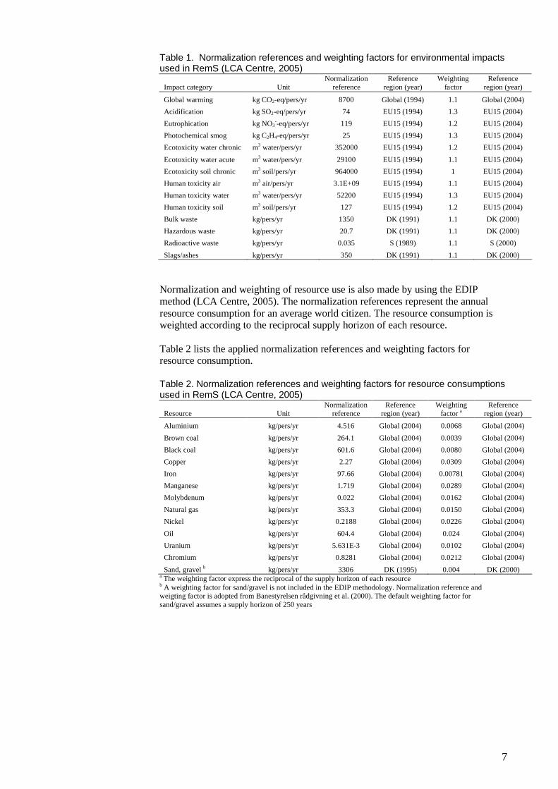
Table 1. Normalization references and weighting factors for environmental impactsused in RemS (LCA Centre, 2005)
Impact category UnitNormalization
referenceReference
region (year)Weighting
factorReference
region (year)
Global warming kg CO2-eq/pers/yr 8700 Global (1994) 1.1 Global (2004)
Acidification kg SO2-eq/pers/yr 74 EU15 (1994) 1.3 EU15 (2004)
Eutrophication kg NO3--eq/pers/yr 119 EU15 (1994) 1.2 EU15 (2004)
Photochemical smog kg C2H4-eq/pers/yr 25 EU15 (1994) 1.3 EU15 (2004)
Ecotoxicity water chronic m3 water/pers/yr 352000 EU15 (1994) 1.2 EU15 (2004)
Ecotoxicity water acute m3 water/pers/yr 29100 EU15 (1994) 1.1 EU15 (2004)
Ecotoxicity soil chronic m3 soil/pers/yr 964000 EU15 (1994) 1 EU15 (2004)
Human toxicity air m3 air/pers/yr 3.1E+09 EU15 (1994) 1.1 EU15 (2004)
Human toxicity water m3 water/pers/yr 52200 EU15 (1994) 1.3 EU15 (2004)
Human toxicity soil m3 soil/pers/yr 127 EU15 (1994) 1.2 EU15 (2004)
Bulk waste kg/pers/yr 1350 DK (1991) 1.1 DK (2000)
Hazardous waste kg/pers/yr 20.7 DK (1991) 1.1 DK (2000)
Radioactive waste kg/pers/yr 0.035 S (1989) 1.1 S (2000)
Slags/ashes kg/pers/yr 350 DK (1991) 1.1 DK (2000)
Normalization and weighting of resource use is also made by using the EDIP method (LCA Centre, 2005). The normalization references represent the annual resource consumption for an average world citizen. The resource consumption is weighted according to the reciprocal supply horizon of each resource.
Table 2 lists the applied normalization references and weighting factors for resource consumption.
Table 2. Normalization references and weighting factors for resource consumptionsused in RemS (LCA Centre, 2005)
Resource UnitNormalization
referenceReference
region (year)Weighting
factor aReference
region (year)
Aluminium kg/pers/yr 4.516 Global (2004) 0.0068 Global (2004)
Brown coal kg/pers/yr 264.1 Global (2004) 0.0039 Global (2004)
Black coal kg/pers/yr 601.6 Global (2004) 0.0080 Global (2004)
Copper kg/pers/yr 2.27 Global (2004) 0.0309 Global (2004)
Iron kg/pers/yr 97.66 Global (2004) 0.00781 Global (2004)
Manganese kg/pers/yr 1.719 Global (2004) 0.0289 Global (2004)
Molybdenum kg/pers/yr 0.022 Global (2004) 0.0162 Global (2004)
Natural gas kg/pers/yr 353.3 Global (2004) 0.0150 Global (2004)
Nickel kg/pers/yr 0.2188 Global (2004) 0.0226 Global (2004)
Oil kg/pers/yr 604.4 Global (2004) 0.024 Global (2004)
Uranium kg/pers/yr 5.631E-3 Global (2004) 0.0102 Global (2004)
Chromium kg/pers/yr 0.8281 Global (2004) 0.0212 Global (2004)
Sand, gravel b kg/pers/yr 3306 DK (1995) 0.004 DK (2000)a The weighting factor express the reciprocal of the supply horizon of each resourceb A weighting factor for sand/gravel is not included in the EDIP methodology. Normalization reference and weigting factor is adopted from Banestyrelsen rådgivning et al. (2000). The default weighting factor for sand/gravel assumes a supply horizon of 250 years

8
REFERENCES
Banestyrelsen rådgivning; HOH Vand og Miljø A/S; NIRAS Rådgivende ingeniører og planlæggere A/S; Revisorsamvirket / Pannell Kerr Forster (2000): Miljørigtig oprensning af forurenede grunde. EU LIFE Project no. 96ENV/DK/0016. Copenhagen, Denmark. Prepared for Banestyrelsen, DSB and Miljøstyrelsen.
Frischknecht, R.; Jungbluth N. (editors) et.al. (2007). Implementation of Life Cycle Impact Assessment Methods. ecoinvent report No. 3. Dübendorf, December 2007.
LCA Center. 2005, List of EDIP factors downloaded from LCA Center Denmark 04-11-2008 at http://www.lca-center.dk/cms/site.aspx?p=1595.
Wenzel, H.; Hauschild M.; Alting L. (1997). Environmental assessment of products - 1: Methodology, tools, and case studies in product development. Chapman & Hall, United Kingdom, 1997, Kluwer Academic Publishers, Hingham, MA. USA.

9
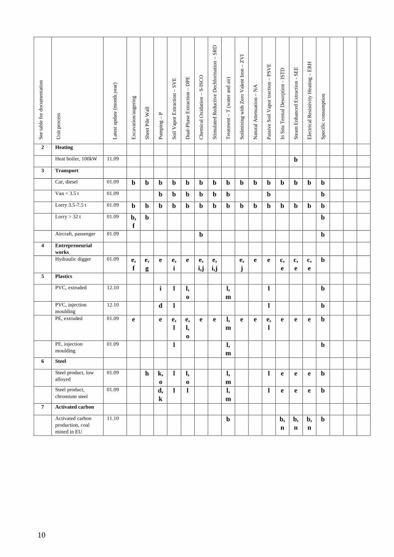
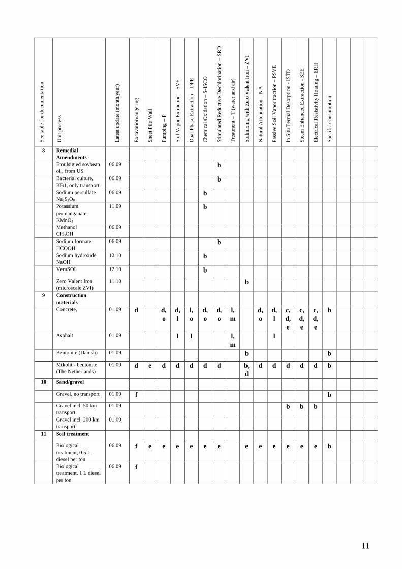
2 Data Sheets - Techniques
An overview of the techniques (T1 - T15) available in RemS and which unit processes are used in the various techniques (see explanation in Notes below table)is shown in Table 1. In addition, the date of the last update of the individual unit processes in RemS is stated.
For documentation of the individual unit processes, see appendix 3.
Table 1. Overview of techniques and use of unit processes in connection with LCA screening calculations(see Notes below table).
See
tab
le f
or d
ocum
enta
tion
Uni
t pr
oces
s
Lat
est
upda
te (
mon
th.y
ear)
Exc
avat
ion/
auge
ring
She
et P
ile
Wal
l
Pum
ping
– P
Soi
l V
apor
Ext
ract
ion
– S
VE
Dua
l-P
hase
Ext
ract
ion
– D
PE
Che
mic
al O
xida
tion
– S
-IS
CO
Sti
mul
ated
Red
ucti
ve D
echlo
rinat
ion –
SR
D
Tre
atm
ent
– T
(w
ater
and
air
)
Soi
lmix
ing
wit
h Z
ero
Val
ent
Iron –
ZV
I
Nat
ural
Att
enua
tion
– N
A
Pas
sive
Soi
l V
apor
tra
ctio
n –
PS
VE
In S
itu
Ter
mal
Des
orpt
ion -
IS
TD
Ste
am E
nhan
ced
Ext
ract
ion -
SE
E
Ele
ctri
cal
Res
isti
vity
Hea
ting –
ER
H
Spe
cifi
c co
nsum
ptio
n
T1
T2
T3
T4
T5
T6
T7
T8
T9
T10
T11
T12
T13
T14
T15
1A Electricity –
consumer mixes
Electricity DK 06.09 m l l m m l d, j
d, j
d, j
a
Electricity DK
(alloc.)
06.09 m l l m m l d,
j
d,
j
d,
j
a
Electricity SE 06.09 m l l m m l d, j
d, j
d, j
a
Electricity NO 06.09 m l l m m l d,
j
d,
j
d,
j
a
Electricity UCTE xx.08 m l l m m l d, j
d, j
d, j
a
Electricity EU27 06.09 m l l m m l d,
j
d,
j
d,
j
a
1B Electricity – single
production tech.
Electricity, coal
(marginal)
11.10 m l l m m l d,
j
d,
j
d,
j
a
Electricity, natural
gas (marginal)
11.10 m l l m m l d,
j
d,
j
d,
j
a
Electricity, wind
power, off shore,
2MW
11.10 m l l m m l d,
j
d,
j
d,
j
a
Electricity, wind
power, on shore,
800 kW
11.10 m l l m m l d,
j
d,
j
d,
j
a
10
See
tab
le f
or
docu
men
tati
on
Unit
pro
cess
Lat
est
updat
e (m
onth
.yea
r)
Exca
vat
ion/a
uger
ing
Shee
t P
ile
Wal
l
Pum
pin
g –
P
Soil
Vap
or
Extr
acti
on –
SV
E
Dual
-Phas
e E
xtr
acti
on –
DP
E
Chem
ical
Oxid
atio
n –
S-I
SC
O
Sti
mula
ted R
educt
ive
Dec
hlo
rinat
ion –
SR
D
Tre
atm
ent
– T
(w
ater
and a
ir)
Soil
mix
ing w
ith Z
ero V
alen
t Ir
on –
ZV
I
Nat
ura
l A
tten
uat
ion –
NA
Pas
sive
Soil
Vap
or
trac
tion –
PS
VE
In S
itu T
erm
al D
esorp
tion -
IS
TD
Ste
am E
nhan
ced E
xtr
acti
on -
SE
E
Ele
ctri
cal
Res
isti
vit
y H
eati
ng –
ER
H
Spec
ific
consu
mpti
on
2 Heating
Heat boiler, 100kW 11.09 b
3 Transport
Car, diesel 01.09 b b b b b b b b b b b b b b b
Van < 3.5 t 01.09 b b b b b b b b
Lorry 3.5-7.5 t 01.09 b b b b b b b b b b b b b b b
Lorry > 32 t 01.09 b,
f
b b
Aircraft, passenger 01.09 b b
4 Entrepreneurial
works
Hydraulic digger 01.09 e,
f
e,
g
e e,
i
e e,
i,j
e,
i,j
e,
j
e e c,
e
c,
e
c,
e
b
5 Plastics
PVC, extruded 12.10 i l l,
o
l,
m
l b
PVC, injection
moulding
12.10 d l l b
PE, extruded 01.09 e e e,
l
e,
l,
o
e e l,
m
e e e,
l
e e e b
PE, injection
moulding
01.09 l l,m
b
6 Steel
Steel product, low
alloyed
01.09 h k,
o
l l,
o
l,
m
l e e e b
Steel product,
chromium steel
01.09 d,
k
l l l,
m
l e e e b
7 Activated carbon
Activated carbon
production, coal
mined in EU
11.10 b b,
n
b,
n
b,
n
b
11
See
tab
le f
or
docu
men
tati
on
Unit
pro
cess
Lat
est
updat
e (m
onth
.yea
r)
Exca
vat
ion/a
uger
ing
Shee
t P
ile
Wal
l
Pum
pin
g –
P
Soil
Vap
or
Extr
acti
on –
SV
E
Dual
-Phas
e E
xtr
acti
on –
DP
E
Chem
ical
Oxid
atio
n –
S-I
SC
O
Sti
mula
ted R
educt
ive
Dec
hlo
rinat
ion –
SR
D
Tre
atm
ent
– T
(w
ater
and a
ir)
Soil
mix
ing w
ith Z
ero V
alen
t Ir
on –
ZV
I
Nat
ura
l A
tten
uat
ion –
NA
Pas
sive
Soil
Vap
or
trac
tion –
PS
VE
In S
itu T
erm
al D
esorp
tion -
IS
TD
Ste
am E
nhan
ced E
xtr
acti
on -
SE
E
Ele
ctri
cal
Res
isti
vit
y H
eati
ng –
ER
H
Spec
ific
consu
mpti
on
8 Remedial
Amendments
Emulsigied soybean
oil, from US
06.09 b
Bacterial culture,
KB1, only transport
06.09 b
Sodium persulfate
Na2S2O8
06.09 b
Potassium
permanganate
KMnO4
11.09 b
Methanol
CH3OH
06.09
Sodium formate
HCOOH
06.09 b
Sodium hydroxide
NaOH
12.10 b
VeruSOL 12.10 b
Zero Valent Iron
(microscale ZVI)
11.10 b
9 Construction
materials
Concrete, 01.09 d d,
o
d,
l
l,
o
d,
o
d,
o
l,
m
d,
o
d,
l
c,
d,e
c,
d,e
c,
d,e
b
Asphalt 01.09 l l l,
m
l
Bentonite (Danish) 01.09 b b
Mikolit - bentonite
(The Netherlands)
01.09 d e d d d d d b,d
d d d d d b
10 Sand/gravel
Gravel, no transport 01.09 f b
Gravel incl. 50 km
transport
01.09 b b b
Gravel incl. 200 km
transport
01.09
11 Soil treatment
Biological
treatment, 0.5 L
diesel per ton
06.09 f e e e e e e e e e e e e b
Biological
treatment, 1 L diesel
per ton
06.09 f
12
Notesa. Entry in sheet 4 LCA-entry combined with choice of type of electricity in sheet 5b. Entry in sheet 4 LCA-entryc. Function of aread. Function of number of wellse. Function of number of meters drilled (investigation wells, pump wells, heating wells, monitoring
wells, etc.)f. Function of amount of soil/soil volumeg. Function of amount of sheet piles, to be usedh. Function of amount of sheet piles disposed or left on sitei. Function of pipe length/length of pipe trenchj. Function of time (machine time, operation time)k. Function of time (life time of plant)l. Function of air flowm. Function of water flown. Function of amount of polluting substanceo. Fixed entries
For the individual techniques are hereinafter given a brief description of how the auto correction of LCA input is for the individual input parameters. Furthermore, it is described which activities are included in the LCA screening calculation.
General conditions and activities such as transport and drilling work in connection with environmental investigations and control investigations are initially described in Section 2.1.
For the individual techniques, the activities are described in Section 2.2.
Specific issues related to transportation, drilling, construction work and other material consumption are described in Section 2.3.
The automatic generation of cost estimates for the individual techniques are described in Section 2.4.
2.1 General information on LCA input data
In connection with LCA inputs, the nominal value of the individual data parameter basically relies on the user input ("User adjusted"). If the user does not make an entry of data, the auto adjusted value will be used. If this is not prepared, the standard value will be used.
Activities included in the LCA screening can either be regulated directly by the user via sheet 4 LCA input, be indirectly dependent on other parameters, or be included as a fixed component that can not be changed by the user.
The automatically adjusted value is typically based on the area and the depth of the contamination in the unsaturated and saturated zone according to the descibtion in sheet 2 Conseptual Model.
Activities such as transportation to and from sites, initial investigations and control investigations are reoccurring activities for the majority of the techniques and are therefore generally described below.
13
2.1.1 The investigation phase
The individual techniques include the investigation phase and the transportation to and from location and construction of screened 6" diameter investigationboreholes.
Input data parameter Formation of auto-adjusted value
Activities included in LCA calculations
Transportation, supervision Transportation by car in connection with supervision
Transportation, rig, lorry, etc. Transportation related to rig,
lorry, etc. The calculation assumes fully utilized payloads (gross weight of vehicle).
Boreholes, 6" diameter with
DN63 mm screen
The standard value multiplied
by the ratio of the standard area and the actual area
(proportional value).
Drilling work related to rig, see
section 2.3.3. Filter-installation with DN63 PEH pipes and
disposal of surplus soil from the borehole to biological soil
treatment, see section 2.3.2.Sealing with 20 kg bentonite (Mikolit) per borehole and
completion in terrain with DN150 mm concrete socket
pipes, see section 2.3.2.
2.1.2 Planning, construction, and operational phases
Transportation activities are in general included in most techniques.
Input data parameter Formation of auto-adjusted
value
Activities included in LCA
calculations
Transportation, supervision
related to the establishment phase
Transportation by car related to
supervision
Transportation, rig, lorry, etc. Transportation related to rig, lorry, etc. The calculation
assumes fully utilized payloads (gross weight of vehicle).
TransportationEngineer truck related to the
establishment phase
Transportation by van/lorry(<3.5 tonnes gross weight)
related to supervision. The calculation assumes fully
utilized payloads (gross weight of vehicle).
TransportationSupervision related to
operation and maintenance
Transportation by car related to supervision and maintenance.
TransportationEngineer truck related to
operation and maintenance
Transportation by van/lorry(<3.5 tonnes gross weight)
related to supervision. The calculation assumes fully utilized payloads (gross weight
of vehicle).
14
2.1.3 Control investigations
Control investigations is included in a number of techniques. Rechecking includes transportation to and from location and construction of boreholes, including collection of control samples. The boreholes are not installed with filter.
Input data parameter Formation of auto-adjusted
value
Activities included in LCA
calculations
Transportation, supervision Transportation ralated to
supervision.
(time)
Transportation per month Monitoring
Total transportation related to supervision in the monitoring
period.
Transportation, rig, lorry, etc. Transportation related to rig, lorry, etc. The calculation
assumes fully utilized payloads (gross weight of vehicle).
Boreholes, 6” diameter without screen
The default value multiplied by the ratio of the standard area and the actual area (propor-
tional value).
Drilling work related to rig, see section 2.3.3. Disposal of surplus soil from the borehole
to biological soil treatment, see section 2.3.2.
Sealing with 20 kg bentonite (Mikolit) per borehole, see
section 2.3.2.
2.2 LCA input data on the individual techniques
2.2.1 Excavation/augering with off site biological treatment
For transportation and drilling work in the investigation phase, see section 2.1.1.
Input data parameter Formation of auto-adjusted
value
Activities included in LCA
calculations
Assumptions for calculations See remarks
Establishment
Excavation and / or augering
Volume of soil to be excavated Sum of volume of "priority 1" pollution in surface soil and in
the unsaturated zone (2 upperlayers of soil, see sheet 2).
Soil handling related to excavation and re-establish-
ment, operation of site, etc., see section 2.3.3.
- Part with narrow/difficult
conditions
Supplement to soil handling,
see section 2.3.3.
- Part with excavation with large diameter auger
Supplement to soil handling, see section 2.3.3.Augering is assumed 3 times as
comprehensive as excavation.
15
Input data parameter Formation of auto-adjusted
value
Activities included in LCA
calculations
Additional soil volume due to
overlap by augering
A standard additional volume
is 20% due to overlap
For the proportion drilled up, a
surcharge of 20% for soil transport, soil handling, and
replacement material is assumed.
Transport and soil handling
Transportation. Supervision Transportation related to supervision.
Biological treatment(class 2 - 4)
Sum of volume of "priority 1" pollution in surface soil and in
the unsaturated zone (2 upper layers of soil, see sheet 2).
Soil handling at off site soil treatment plant – half of which
equivalent to 1,000 mg / kg light oil and half equivalent to
2,000 mg / kg light oil.
- Transport, exclusive return driving
Transport of soil to soil treatment plant on large lorry(>32 tonnes gross weight) incl.
return transportation.
Replacement materials and
filling in
Sand and gravel (new
materials)
The standard value multiplied
by the ratio of the standard volume and the actual volume
of excavated soil (proportional value).
Use of sand and gravel as a
function of excavated volume of soil.
Remarks:If part of the excavated soil should not be removed for soil remediation, this deduction shall be made in the input data of soil volume for soil remediation.
Soil Treatment includes only biological soil treatment on soil treatment plants in Denmark. The unit processes used are based on treatment of lighter oils such as gasoline, kerosene and gas oil. If other form of soil treatment is desired, this should be noted.
Use of recycled materials of sand, gravel or crushed concrete can not be handled in RemS at present. In the event of total or partial back fill with recycled materials (e.g. approved re-filling of slightly polluted soil), this should be noted separately.
Evaporation of pollutants into the atmosphere is not included in the LCA calculation.
It is presumed that 50% of the soil that are transported to soil treatment plant will be reused and 50 % will be final landfilled which is included as bulk waste in the LCA calculation.
16
2.2.2 Sheet Pile Wall
For transportation in the investigation phase, see 2.1.1.
Input data parameter Formation of auto-adjusted value
Activities included in LCA calculations
Assumptions for calculations
Depth of excavation Assumed equivalent to the lower delineation of the pollution in the unsaturated
zone for "priority 1" pollution in the source area, see sheet 2).
Investigations (geotechnics) Assumed one geotechnical
borehole per 10 m sheet piling. Drilling depth to depth of sheet
piling.
Drilling work related to rig, see
section 2.3.3. Installation of filter with DN25 mm filter and
disposal of surplus soil from the borehole to biological soil treatment, see section 2.3.2.
Sealing with bentonite (Mikolit), see section 2.3.2.
Construction (hammer driving
or pressing down pile wall)
Transportation. Truck with ram
(return).
Transport by big lorry (>32
tonnes gross weight)
Trapeze wall - continuous
steel wall
Length Assumed equivalent to the
periphery of a circular area for “priority 2” pollution in the source area, see sheet 2.
Piling depth Assumed 2.5 times the depth of the excavation.
Steel profile See remarks
HE profile wall –
discontinuous steel profiles
Length As for trapeze wall
Piling depth Assumed 3.0 times the depth of the excavation.
Distance between steel profiles
Steel profile See remarks
Total weight of wall Sum of trapeze wall and / orHE profile wall.
Contractor’s work assuming a pile driving of 5 tonnes of
sheet wall per hour. Fuel consumption, see section
2.3.3
Draw back of sheet pile wall Contractor’s work assuming
drawing up of 5 tonnes of sheet wall per hour. Fuel consumption, see section
2.3.3Parts of wall left and part of
wall to be disposed of are included in the LCA
calculation as use of steel.
17
Remarks:Users must specify the type of sheet piling as weight/m2 wall. Usually only one of the listed wall types is used. For the wall type not used, a length of 0 m is indicated.
2.2.3 Pumping – P
Regarding transportation in the investigation phase, see section 2.1.1. For transportation in the construction and operation phases, see section 2.1.2.
Input data parameter Formation of auto-adjusted value
Activities included in LCA calculations
Assumptions for calculations
Source area +plume area in the secondary aquifer
Actual area of ”priority 1” pollution in the secondary
groundwater aquifer(calculated as total area in the
source area and plume area, see sheet 2)
Depth to bottom of plume insecondary aquifer
Actual maximum depth to the bottom of the water pollution
in the source area or in the plume area, see sheet 2.
Plume area in primary aquifer Actual area of ”priority 1” pollution in the primary groundwater aquifer
(calculated as total area in the source area and plume area,
see sheet 2)
Depth to bottom of plume in
primary aquifer
Actual maximum depth to the
bottom of the water pollution in the source area or in the
plume area, see sheet 2.
Investigations
Boreholes, secondary aquifer,6" diameter with DN63 mm screen
Standard value multiplied by the ratio of the standard area of source + plume and the actual
area of source + plume (proportional value).
Drilling work related to rig, see section 2.3.3. Filter-installation with DN63 PEH pipes and
disposal of surplus soil from the borehole to biological soil
treatment, see section 2.3.2.Sealing with 20 kg bentonite
(Mikolit) per borehole and completion in terrain with DN150 mm concrete socket
pipes, see section 2.3.2.
Boreholes, primary aquifer,
8" diameter with DN110 mm screen
Standard value multiplied by
the ratio of the standard area of source + plume and the actual
area of source + plume (proportional value).
Drilling work related to rig, see
section 2.3.3. Filter-installation with DN110 PEH pipes and
disposal of surplus soil from the borehole to biological soil
treatment, see section 2.3.2.Sealing with 30 kg bentonite (Mikolit) per borehole and
completion in terrain with DN200 mm concrete socket
pipes, see section 2.3.2.
Establishment and operation
Time of operation
Pumping system:
Secondary=0, Primary=1
User must chose pumping from
the secondary (0) or the primary aquifer (1).
18
Input data parameter Formation of auto-adjusted
value
Activities included in LCA
calculations
Pumping system – secondary
ground water
Pumping wells, 10" diameter
with DN125 mm screen
Drilling work related to rig, see
section 2.3.3. Filter-installation with DN125 PEH pipes and disposal of surplus soil from
the borehole to biological soil treatment, see section 2.3.2.
Sealing with 50 kg bentonite (Mikolit) per well, see section
2.3.2. Completion in terrain with DN1250 mm concrete well.
Use of pumps, stainless steel with a lifetime of 5 years.
Total pump yield
Pump pipe, DN75 PVC Use of DN75 PVC
Power consumption for raw water pumps
Calculation based on linear interpolation between a power
consumption of 1.5 kW at 2.5 m3/h and 2.5 kW at 7 m3/h.
Calculation based on a power
consumption corresponding to Grundfos SP3A-15 and SP8A-15.
Total power consumption for the total operation period
Power consumption as a function of the water flow
Pump system – primary ground water
Pumping wells, 12" diameter with DN160mm screen
Drilling work related to rig, see section 2.3.3. Filter-installation
with DN160 PEH pipes and disposal of surplus soil from
the borehole to biological soil treatment, see section 2.3.2.Sealing with 100 kg bentonite
(Mikolit) per well, see section 2.3.2. Completion in terrain
with DN2000 mm concrete well.
Use of pumps, stainless steel with a lifetime of 5 years.
Total pump yield
Pump pipe, DN110 PVC Use of DN110 PVC
Power consumption for raw water pumps
Calculation based on linear interpolation between a power consumption of 1.5 kW at 2.5
m3/h and 2.5 kW at 7 m3/h.
Calculation based on a power consumption corresponding to
Grundfos SP3A-15 and SP8A-15.
Total power consumption for the total operation period
Power consumption as a function of water flow.

19
Remarks:For each technique is included 1 m2 in situ concrete surfacing (fixed amount) for various endings.
If water treatment is to be performed, the treatment plant must be chosen as a separate technique.
2.2.4 Soil Vapor Extraction – SVE
Regarding transportation in the investigation phase, see section 2.1.1. For services in the construction and operation phases, see section 2.1.2. For control investigations, see section 2.1.3.
Input data parameter Formation of auto-adjusted value
Activities included in LCA calculations
Assumptions for calculations
Remediation area in the
unsaturated zone
Actual area of ”priority 1”
pollution in the secondary groundwater aquifer(calculated as total area in the
source area and plume area, see sheet 2)
Depth to top of gas plume Actual depth to top of gas plume in unsaturated zone, see
sheet 2.
Depth to bottom of gas plume Actual depth to bottum of gas
plume in unsaturated zone, see sheet 2.
Total soil gas volume in gas plume
Actual volume and an air porosity of 0.3.
Investigations
Establishment and operation
Extraction wells - DN63mm Assumed 1 extraction well per
200 m2 of the soil gas pollution plume.
Drilling work related to rig, see
section 2.3.3. Filter-installation with DN63 PEH pipes and disposal of surplus soil from
the borehole to biological soil treatment, see section 2.3.2.
Sealing with 20 kg bentonite (Mikolit) per well, see section
2.3.2. Completion in terrain with DN1250 mm concrete well. Digging of 25 m pipe
trench per well.
Depth of extraction wells Assumed corresponding to the
lower delineation of the calculated value of soil gas
pollution cleaned up.
Number of air shifts in the
formation
Time of operation
Alternating operation, operation part
Air flow during extraction Equivalent to the number of air shifts for the total soil gas
volume, operation time, and alternating operation, if any.
Material consumption (asfunction of air flow) for the
plant, comprising PVC pipes, PE, steel, stainless steel, and concrete and asphalt paving.
20
Input data parameter Formation of auto-adjusted
value
Activities included in LCA
calculations
Consumption of electricity per
year
Calculation based on linear
interpolation between a power consumption of 12,500
kWh/year at 100 m3/h and 25,000 kWh/year at 200 m3/h.
Power consumption as function
of air flow
Remarks:If air treatment is to be performed, the treatment plant must be chosen as a separate technique.
2.2.5 Dual-Phase Extraction – DPE
Regarding transportation in the investigation phase, see section 2.1.1. For services in the construction and operation phases, see section 2.1.2.
Input data parameter Formation of auto-adjusted value
Activities included in LCA calculations
Assumptions for calculations
Source area in secondary
aquifer
Actual area of ”priority 1”
pollution in secondary groundwater aquifer
(calculated as total area in the source area, see sheet 2)
Remediation depth in secondary aquifer
Actuel depth to saturated zone i source area, see sheet 2.
Remediation depth in primary aquifer
Actuel depth to top of primary aquifer i source area, see sheet2.
Investigations
Boreholes, secondary aquifer,
6" diameter with DN63 mm screen
Standard value multiplied by
the ratio of the standard area of source + plume and the actual
area of source + plume (proportional value).
Drilling work related to rig, see
section 2.3.3. Filter-installation with DN63 PEH pipes and
disposal of surplus soil from the borehole to biological soil
treatment, see section 2.3.2.Sealing with 20 kg bentonite (Mikolit) per borehole and
completion in terrain with DN150 mm concrete socket
pipes, see section 2.3.2.
Boreholes, primary aquifer,
8" diameter with DN110 mm screen
Standard value multiplied by
the ratio of the standard area of source + plume and the actual
area of source + plume (proportional value).
Drilling work related to rig, see
section 2.3.3. Filter-installation with DN110 PEH pipes and
disposal of surplus soil from the borehole to biological soil treatment, see section 2.3.2.
Sealing with 30 kg bentonite (Mikolit) per borehole and
completion in terrain with DN200 mm concrete socket
pipes, see section 2.3.2.
Establishment and operation
Pumping system
Time of operation
21
Input data parameter Formation of auto-adjusted
value
Activities included in LCA
calculations
Pumping wells ~ DN63 mm
PEH filters
Number of pumping wells
assumed at 1 ea per 100 m2.
Drilling work related to rig, see
section 2.3.3. Filter-installation with DN63 PEH pipes and
disposal of surplus soil from the borehole to biological soil treatment, see section 2.3.2.
Sealing with 20 kg bentonite (Mikolit) per well, see section
2.3.2. Completion in terrain with DN1250 mm concrete
well.
Total pumping yield, air The total pump yield is calculated as number of pump
wells x pump yield per well. The pump yield per well is
assumed at 10 m3/hour.
Material consumption (as a function of air flow) for the
plant, comprising PVC pipes, steel, stainless steel, and
concrete and asphalt paving.
Total pumping yield, water The total pump yield is
calculated as number of pump wells x pump yield per well.
The pump yield per well is assumed at 0.25 m3/hour.
Consumption of electricity -vacuum pump
Calculation based on linear interpolation between a power consumption of 2.5 kW/year at
50 m3/h and 4 kW at 100 m3/h.
The calculation is based on power consumption corre-
sponding to a Sterling liquid ring pump.
Power consumption as a function of air flow.
Remarks:If air or water treatment is to be performed, the treatment plant must be chosen as a separate technique.
2.2.6 Surfactant-enhanced In Situ Chemical Oxidation – S-ISCO
Regarding transportation in the investigation phase, see section 2.1.1. For services in the construction and operation phases, see section 2.1.2. For control investigations, see section 2.1.3.
Input data parameter Formation of auto-adjusted value
Activities included in LCA calculations
Assumptions for calculations
Remediation area Actual area of ”priority 1”
pollution in secondary groundwater aquifer(calculated as total area in the
source area, see sheet 2)
Thickness of remediation
interval
Actual thickness of secondary
groundwater aquifer in source area, see sheet 2.
Depth to bottom of plume in secondary aquifer
Actual maximum depth to bottom of plume in secondary
aquifer in source area or plume area, see sheet 2.
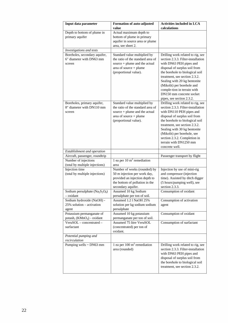
22
Input data parameter Formation of auto-adjusted
value
Activities included in LCA
calculations
Depth to bottom of plume in
primary aquifer
Actual maximum depth to
bottom of plume in primary aquifer in source area or plume
area, see sheet 2.
Investigations and tests
Boreholes, secondary aquifer, 6" diameter with DN63 mm screen
Standard value multiplied by the ratio of the standard area of source + plume and the actual
area of source + plume (proportional value).
Drilling work related to rig, see section 2.3.3. Filter-installation with DN63 PEH pipes and
disposal of surplus soil from the borehole to biological soil
treatment, see section 2.3.2.Sealing with 20 kg bentonite
(Mikolit) per borehole and comple-tion in terrain with DN150 mm concrete socket
pipes, see section 2.3.2.
Boreholes, primary aquifer,
8" diameter with DN110 mm screen
Standard value multiplied by
the ratio of the standard area of source + plume and the actual
area of source + plume (proportional value).
Drilling work related to rig, see
section 2.3.3. Filter-installation with DN110 PEH pipes and
disposal of surplus soil from the borehole to biological soil
treatment, see section 2.3.2.Sealing with 30 kg bentonite (Mikolit) per borehole, see
section 2.3.2. Completion in terrain with DN1250 mm
concrete well.
Establishment and operation
Aircraft, passenger, roundtrip Passenger transport by flight
Number of injections
(total by multiple injections)
1 ea per 10 m2 remediation
area
Injection time
(total by multiple injections)
Number of weeks (rounded) by
50 m injection per work day, provided an injection depth to
the bottom of pollution in the secondary aquifer.
Injection by use of mini-rig
and compressor (injection time). Assisted by ditch digger
(5 hours/pumping well), see section 2.3.3.
Sodium persulphate (Na2S2O8)
– oxidant
Assumed 10 kg Sodium
persulphate per ton of soil.
Consumption of oxidant
Sodium hydroxide (NaOH) -
25% solution – activationagent
Assumed 1.2 l NaOH 25%
solution per kg sodium sodium persulphate
Consumption of activation
agent
Potassium permanganate of potash, (KMnO4) - oxidant
Assumed 10 kg potassium permanganate per ton of soil.
Consumption of oxidant
VeruSOL – concentrated –surfactant
Assumed 75 litre VeruSOL (concentrated) per ton of
oxidant.
Consumption of surfactant
Potential pumping and
recirculation
Pumping wells ~ DN63 mm 1 ea per 100 m2 remediation
area (rounded)
Drilling work related to rig, see
section 2.3.3. Filter-installation with DN63 PEH pipes and disposal of surplus soil from
the borehole to biological soil treatment, see section 2.3.2.
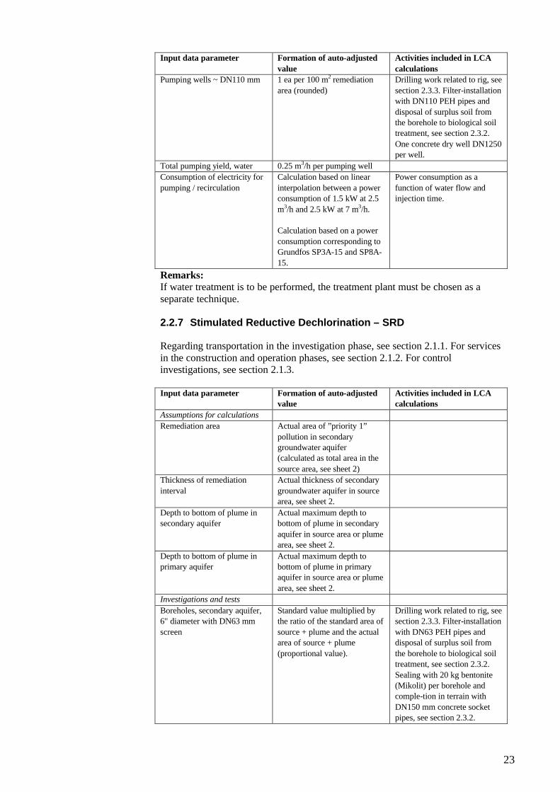
23
Input data parameter Formation of auto-adjusted
value
Activities included in LCA
calculations
Pumping wells ~ DN110 mm 1 ea per 100 m2 remediation
area (rounded)
Drilling work related to rig, see
section 2.3.3. Filter-installation with DN110 PEH pipes and
disposal of surplus soil from the borehole to biological soil treatment, see section 2.3.2.
One concrete dry well DN1250per well.
Total pumping yield, water 0.25 m3/h per pumping well
Consumption of electricity for
pumping / recirculation
Calculation based on linear
interpolation between a power consumption of 1.5 kW at 2.5
m3/h and 2.5 kW at 7 m3/h.
Calculation based on a power
consumption corresponding to Grundfos SP3A-15 and SP8A-
15.
Power consumption as a
function of water flow and injection time.
Remarks:If water treatment is to be performed, the treatment plant must be chosen as a separate technique.
2.2.7 Stimulated Reductive Dechlorination – SRD
Regarding transportation in the investigation phase, see section 2.1.1. For services in the construction and operation phases, see section 2.1.2. For control investigations, see section 2.1.3.
Input data parameter Formation of auto-adjusted value
Activities included in LCA calculations
Assumptions for calculations
Remediation area Actual area of ”priority 1”
pollution in secondary groundwater aquifer(calculated as total area in the
source area, see sheet 2)
Thickness of remediation
interval
Actual thickness of secondary
groundwater aquifer in source area, see sheet 2.
Depth to bottom of plume in secondary aquifer
Actual maximum depth to bottom of plume in secondary
aquifer in source area or plume area, see sheet 2.
Depth to bottom of plume in primary aquifer
Actual maximum depth to bottom of plume in primary aquifer in source area or plume
area, see sheet 2.
Investigations and tests
Boreholes, secondary aquifer, 6" diameter with DN63 mm
screen
Standard value multiplied by the ratio of the standard area of
source + plume and the actual area of source + plume
(proportional value).
Drilling work related to rig, see section 2.3.3. Filter-installation
with DN63 PEH pipes and disposal of surplus soil from
the borehole to biological soil treatment, see section 2.3.2.
Sealing with 20 kg bentonite (Mikolit) per borehole and comple-tion in terrain with
DN150 mm concrete socket pipes, see section 2.3.2.
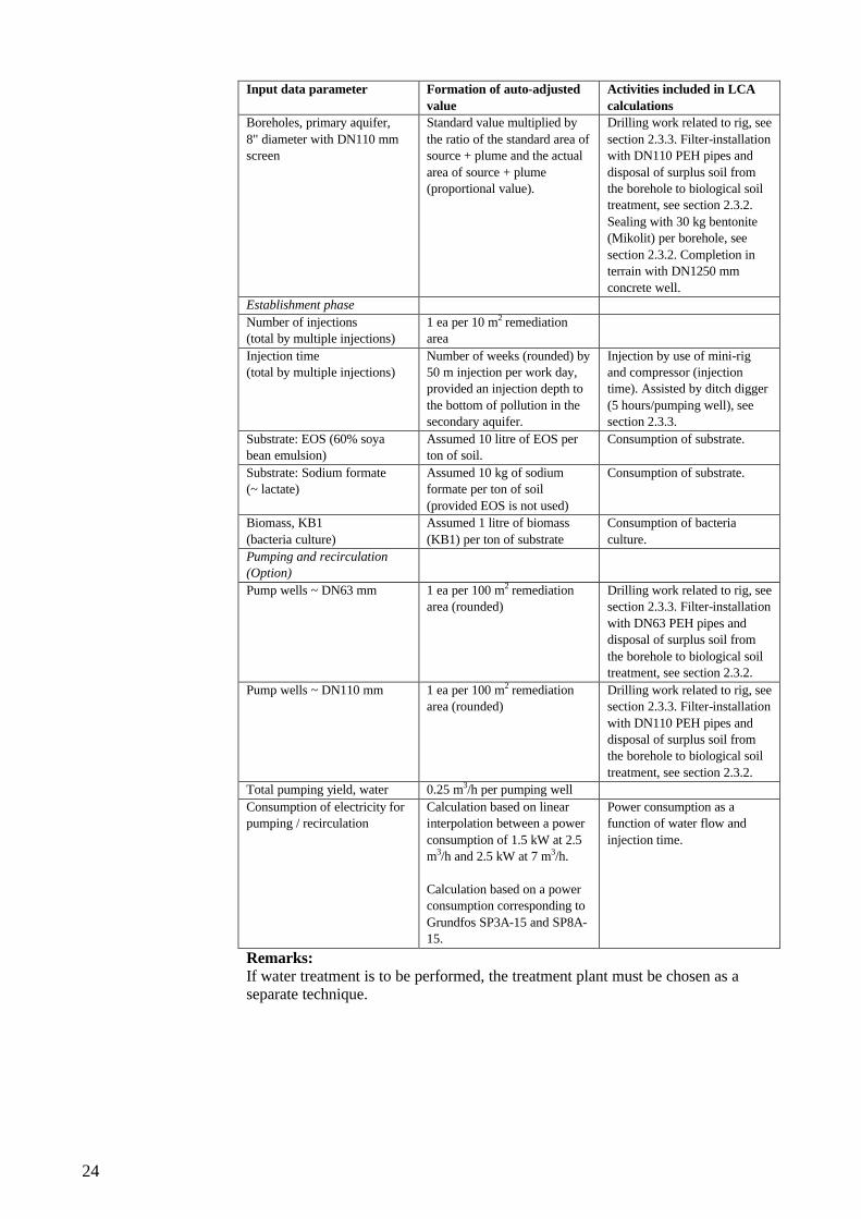
24
Input data parameter Formation of auto-adjusted
value
Activities included in LCA
calculations
Boreholes, primary aquifer,
8" diameter with DN110 mm screen
Standard value multiplied by
the ratio of the standard area of source + plume and the actual
area of source + plume (proportional value).
Drilling work related to rig, see
section 2.3.3. Filter-installation with DN110 PEH pipes and
disposal of surplus soil from the borehole to biological soil treatment, see section 2.3.2.
Sealing with 30 kg bentonite (Mikolit) per borehole, see
section 2.3.2. Completion in terrain with DN1250 mm
concrete well.
Establishment phase
Number of injections (total by multiple injections)
1 ea per 10 m2 remediationarea
Injection time (total by multiple injections)
Number of weeks (rounded) by 50 m injection per work day, provided an injection depth to
the bottom of pollution in the secondary aquifer.
Injection by use of mini-rig and compressor (injection time). Assisted by ditch digger
(5 hours/pumping well), see section 2.3.3.
Substrate: EOS (60% soya bean emulsion)
Assumed 10 litre of EOS per ton of soil.
Consumption of substrate.
Substrate: Sodium formate (~ lactate)
Assumed 10 kg of sodium formate per ton of soil
(provided EOS is not used)
Consumption of substrate.
Biomass, KB1
(bacteria culture)
Assumed 1 litre of biomass
(KB1) per ton of substrate
Consumption of bacteria
culture.
Pumping and recirculation(Option)
Pump wells ~ DN63 mm 1 ea per 100 m2 remediationarea (rounded)
Drilling work related to rig, see section 2.3.3. Filter-installation
with DN63 PEH pipes and disposal of surplus soil from
the borehole to biological soil treatment, see section 2.3.2.
Pump wells ~ DN110 mm 1 ea per 100 m2 remediationarea (rounded)
Drilling work related to rig, see section 2.3.3. Filter-installation
with DN110 PEH pipes and disposal of surplus soil from the borehole to biological soil
treatment, see section 2.3.2.
Total pumping yield, water 0.25 m3/h per pumping well
Consumption of electricity for pumping / recirculation
Calculation based on linear interpolation between a power
consumption of 1.5 kW at 2.5 m3/h and 2.5 kW at 7 m3/h.
Calculation based on a power consumption corresponding to
Grundfos SP3A-15 and SP8A-15.
Power consumption as a function of water flow and
injection time.
Remarks:If water treatment is to be performed, the treatment plant must be chosen as a separate technique.

25
2.2.8 Treatment – T (water and air)
Regarding transportation in the investigation phase, see section 2.1.1.
Input data parameter Formation of auto-adjusted
value
Activities included in LCA
calculations
Operation
Time of operation
Oil separator (Yes=1, No=0) User must choose (1) or not
choose (0) oil separator
Oil separator and grit
trap(Plastic-PE) < 20 m3/h
Dead load of oil separator and
grit trap.
Oil separator and grit
trap(concrete) < 20 m3/h
Dead load of oil separator and
grit trap.
Water treatment (Yes=1,
No=0):
User must choose (1) or not
choose (0) water treatment
Capacity
Consumption of electricity excl. aeration of water
Calculation based on linear interpolation between a power
consumption of 15,000 kWh/year at 10 m3/h and 20,000 kWh/year at 20 m3/h.
Power consumption as a function of water flow.
Activated carbon – GAC (on
water) - consumption
Calculation based on linear
interpolation between a coal consumption of 100 kg/year at
10 m3/h and 200 kg/year at 20 m3/h.
Consumption of activated
carbon.
In building=1; In container=2 User must choose whether the treatment plant to be
established in building (1) or in container (2)
Material consumption for building and container, incl.
treatment plant, is included (as a function of air flow) for plant
comprising PVC pipes, PE, steel, stainless steel, and
concrete and asphalt paving.
Air treatment – aerated water
(Yes=1, No=0):
User must choose (1) or not
choose (0) water treatment by aeration
Capacity (air stripping -INKA system)
The value is 150 times the amount of water for water treatment.
This assumption is based on an assumed need of aeration of
50-200 times the amount of water treated.
Consumption of electricity, air stripping
Value based on linear interpolation between a power
consumption of 175,000 kWh/year at 1,000 m3/h and 300,000 kWh/year at 2.500
m3/h.
Power consumption as a function of air flow.
Activated carbon – GAC (on air) - consumption
Calculation based on linear interpolation between a coal
consumption of 50 kg/year at 10 m3/h and 100 kg/year at 20
m3/h.
Consumption of activated carbon.
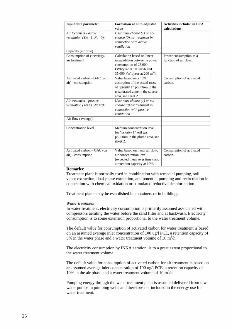
26
Input data parameter Formation of auto-adjusted
value
Activities included in LCA
calculations
Air treatment - active
ventilation (Yes=1, No=0):
User must choose (1) or not
choose (0) air treatment in connection with active
ventilation
Capacity (air flow)
Consumption of electricity, air treatment
Calculation based on linear interpolation between a power consumption of 25,000
kWh/year at 100 m3/h and 35.000 kWh/year at 200 m3/h.
Power consumption as a function of air flow.
Activated carbon - GAC (on air) - consumption
Value based on a 10% absorption of the actual mass
of ”prority 1” pollution in the unsaturated zone in the source
area, see sheet 2.
Consumption of activated carbon.
Air treatment - passive ventilation (Yes=1, No=0):
User must choose (1) or not choose (0) air treatment in
connection with passive ventilation
Air flow (average)
Concentration level Medium concentration levelfor "priority 1" soil gas
pollution in the plume area, see sheet 2.
Activated carbon – GAC (on
air) - consumption
Value based on mean air flow,
air concentration level(expected mean over time), and a retention capacity at 10%.
Consumption of activated
carbon.
Remarks:Treatment plant is normally used in combination with remedial pumping, soil vapor extraction, dual-phase extraction, and potential pumping and recirculation in connection with chemical oxidation or stimulated reductive dechlorination.
Treatment plants may be established in containers or in buildings.
Water treatmentIn water treatment, electricity consumption is primarily assumed associated with compressors aerating the water before the sand filter and at backwash. Electricityconsumption is to some extension proportional to the water treatment volume.
The default value for consumption of activated carbon for water treatment is based on an assumed average inlet concentration of 100 ug/l PCE, a retention capacity of 5% in the water phase and a water treatment volume of 10 m3/h.
The electricity consumption by INKA aeration, is to a great extent proportional to the water treatment volume.
The default value for consumption of activated carbon for air treatment is based on an assumed average inlet concentration of 100 ug/l PCE, a retention capacity of 10% in the air phase and a water treatment volume of 10 m3/h.
Pumping energy through the water treatment plant is assumed delivered from raw water pumps in pumping wells and therefore not included in the energy use for water treatment.
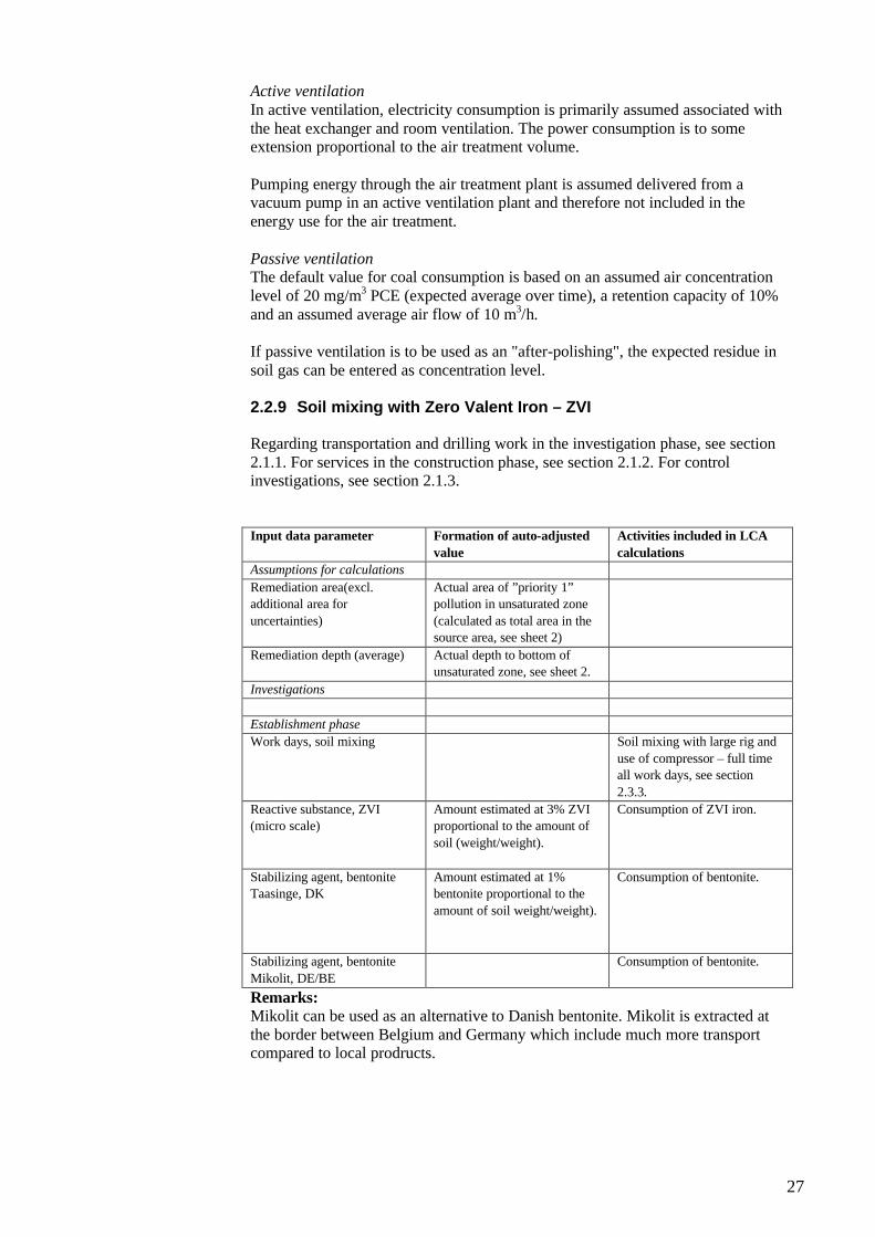
27
Active ventilationIn active ventilation, electricity consumption is primarily assumed associated with the heat exchanger and room ventilation. The power consumption is to some extension proportional to the air treatment volume.
Pumping energy through the air treatment plant is assumed delivered from a vacuum pump in an active ventilation plant and therefore not included in the energy use for the air treatment.
Passive ventilationThe default value for coal consumption is based on an assumed air concentration level of 20 mg/m3 PCE (expected average over time), a retention capacity of 10% and an assumed average air flow of 10 m3/h.
If passive ventilation is to be used as an "after-polishing", the expected residue in soil gas can be entered as concentration level.
2.2.9 Soil mixing with Zero Valent Iron – ZVI
Regarding transportation and drilling work in the investigation phase, see section 2.1.1. For services in the construction phase, see section 2.1.2. For control investigations, see section 2.1.3.
Input data parameter Formation of auto-adjusted
value
Activities included in LCA
calculations
Assumptions for calculations
Remediation area(excl.additional area for
uncertainties)
Actual area of ”priority 1” pollution in unsaturated zone
(calculated as total area in the source area, see sheet 2)
Remediation depth (average) Actual depth to bottom of unsaturated zone, see sheet 2.
Investigations
Establishment phase
Work days, soil mixing Soil mixing with large rig and
use of compressor – full time all work days, see section
2.3.3.
Reactive substance, ZVI (micro scale)
Amount estimated at 3% ZVI proportional to the amount of
soil (weight/weight).
Consumption of ZVI iron.
Stabilizing agent, bentonite Taasinge, DK
Amount estimated at 1% bentonite proportional to the
amount of soil weight/weight).
Consumption of bentonite.
Stabilizing agent, bentonite
Mikolit, DE/BE
Consumption of bentonite.
Remarks:Mikolit can be used as an alternative to Danish bentonite. Mikolit is extracted at the border between Belgium and Germany which include much more transport compared to local prodructs.
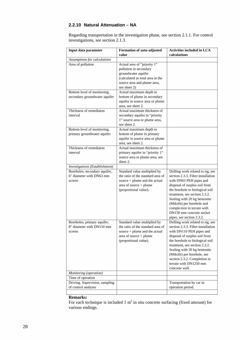
28
2.2.10 Natural Attenuation – NA
Regarding transportation in the investigation phase, see section 2.1.1. For control investigations, see section 2.1.3.
Input data parameter Formation of auto-adjusted value
Activities included in LCA calculations
Assumptions for calculations
Area of pollution Actual area of ”priority 1” pollution in secondary groundwater aquifer
(calculated as total area in the source area and plume area,
see sheet 2)
Bottom level of monitoring,
secondary groundwater aquifer
Actual maximum depth to
bottom of plume in secondary aquifer in source area or plume
area, see sheet 2.
Thickness of remediaton interval
Actual maximum thickness of secondary aquifer in “priority
1” source area or plume area, see sheet 2.
Bottom level of monitoring, primary groundwater aquifer
Actual maximum depth to bottom of plume in primary
aquifer in source area or plume area, see sheet 2.
Thickness of remediaton interval
Actual maximum thickness of primary aquifer in “priority 1”
source area or plume area, see sheet 2.
Investigations (Establishment)
Boreholes, secondary aquifer, 6" diameter with DN63 mm
screen
Standard value multiplied by the ratio of the standard area of
source + plume and the actual area of source + plume
(proportional value).
Drilling work related to rig, see section 2.3.3. Filter-installation
with DN63 PEH pipes and disposal of surplus soil from
the borehole to biological soil treatment, see section 2.3.2.
Sealing with 20 kg bentonite (Mikolit) per borehole and comple-tion in terrain with
DN150 mm concrete socket pipes, see section 2.3.2.
Boreholes, primary aquifer, 8" diameter with DN110 mm
screen
Standard value multiplied by the ratio of the standard area of
source + plume and the actual area of source + plume
(proportional value).
Drilling work related to rig, see section 2.3.3. Filter-installation
with DN110 PEH pipes and disposal of surplus soil from
the borehole to biological soil treatment, see section 2.3.2.Sealing with 30 kg bentonite
(Mikolit) per borehole, see section 2.3.2. Completion in
terrain with DN1250 mm concrete well.
Monitoring (operation)
Time of operation
Driving. Supervision, sampling of control analyses
Transportation by car in operation period.
Remarks:For each technique is included 1 m2 in situ concrete surfacing (fixed amount) for various endings.
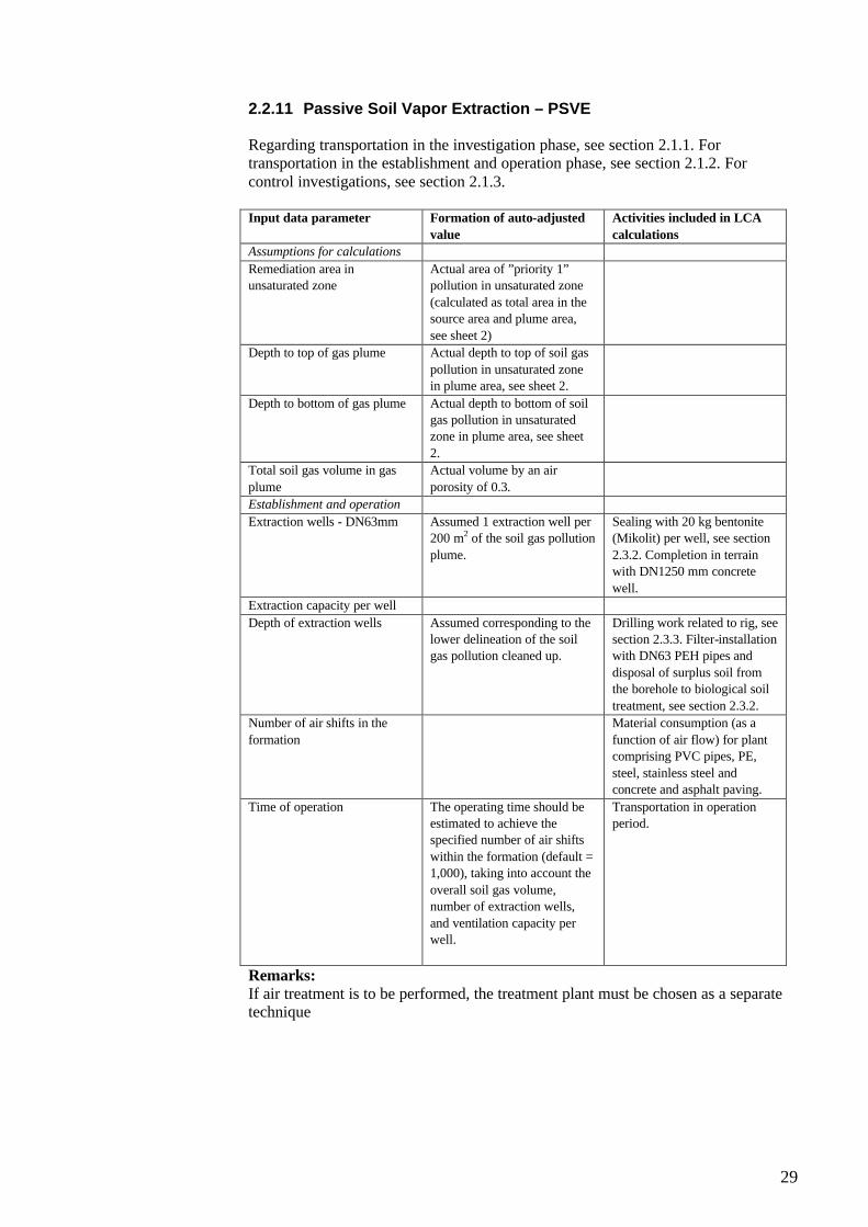
29
2.2.11 Passive Soil Vapor Extraction – PSVE
Regarding transportation in the investigation phase, see section 2.1.1. For transportation in the establishment and operation phase, see section 2.1.2. For control investigations, see section 2.1.3.
Input data parameter Formation of auto-adjusted
value
Activities included in LCA
calculations
Assumptions for calculations
Remediation area in unsaturated zone
Actual area of ”priority 1” pollution in unsaturated zone
(calculated as total area in the source area and plume area,
see sheet 2)
Depth to top of gas plume Actual depth to top of soil gas
pollution in unsaturated zone in plume area, see sheet 2.
Depth to bottom of gas plume Actual depth to bottom of soil gas pollution in unsaturated zone in plume area, see sheet
2.
Total soil gas volume in gas
plume
Actual volume by an air
porosity of 0.3.
Establishment and operation
Extraction wells - DN63mm Assumed 1 extraction well per 200 m2 of the soil gas pollution
plume.
Sealing with 20 kg bentonite (Mikolit) per well, see section
2.3.2. Completion in terrain with DN1250 mm concrete
well.
Extraction capacity per well
Depth of extraction wells Assumed corresponding to the lower delineation of the soil gas pollution cleaned up.
Drilling work related to rig, see section 2.3.3. Filter-installation with DN63 PEH pipes and
disposal of surplus soil from the borehole to biological soil
treatment, see section 2.3.2.
Number of air shifts in the
formation
Material consumption (as a
function of air flow) for plant comprising PVC pipes, PE,
steel, stainless steel and concrete and asphalt paving.
Time of operation The operating time should be estimated to achieve the specified number of air shifts
within the formation (default = 1,000), taking into account the
overall soil gas volume, number of extraction wells,
and ventilation capacity per well.
Transportation in operation period.
Remarks:If air treatment is to be performed, the treatment plant must be chosen as a separate technique

30
2.2.12 In Situ Termal Desorption - ISTD (conductive heating)
For transportation and boreholes in the investigation phase, see section 2.1.1. For transportation in the establishment and operation phase, see section 2.1.2. For control investigations, see section 2.1.3.
Input data parameter Formation of auto-adjusted value
Activities included in LCA calculations
Assumptions for calculations
Remediation area(without
additional area for uncertainties)
Actual area of ”priority 1”
pollution in unsaturated zone (calculated as total area in the
source area, see sheet 2)
Use of trench digger 37 hours/
500 m2.
Remediation depth (average) Actual depth to bottom of unsaturated zone, see sheet 2.
Establishment
Depth to top level to be heated(average)
Depth to bottom level to be
heated (average)
Value is remediation depth +
1,5 m
Heating wells, Direct Push, DN89 Heatercan
Calculated as 10 ea + 1 ea per 15 m2
Mini-rig 1 hour per heating well. 18 kg of steel and 1 kg of
stainless steel per m well.Heating elements 1.3 kg of
stainless steel per m well.
Temperature monitoring
probes, Direct Push, 1" screen
Calculated as 5 ea + 1/5 of
number of heating wells
Mini-rig 1 hour per sounding
point. 3 kg of steel and 5.5 kgof concrete per m sounding.
Vacuum venting wells, 8" Calculated as 3 ea + 1/4 of
number of heating wells
Drilling work related to rig, see
section 2.3.3. Disposal of surplus soil from the borehole
to biological soil treatment, see section 2.3.2. Filter-installation
consisting of 3.5 kg stainless steel and 5.4 steel per m well.
Sealing with 140 kg concrete per well. Consumption of steel for connection pipe from
vacuum extraction 160 m of 40 kg/m.
Pressure monitoring probes, 1 m deep, 1” screen
Calculated as 3 ea + 1/15 of number of heating wells
Mini-rig 1 hour per sounding point. 5 kg of steel per m
sounding.
Vapor drain – sand/gravel
layer
Calculated as heating area x
0.1 m thickness
Consumption of sand and
gravel.
Vaporcap, foamed concrete(~400 kg/m3, 0.2 m thick)
Calculated as heating area x 0.2 m thickness
Consumption of concrete.
Operation
Consumption of electricity for soil heating
Power consumption is calculated on basis of a power
consumption of 300 kWh/m3 soil multiplied by remediation
volume.
Power consumption as a function of remediation
volume.
Time of operation
Operating power for other electrical units
Value is estimated at 30kW+1kW/10 m2
remediation area
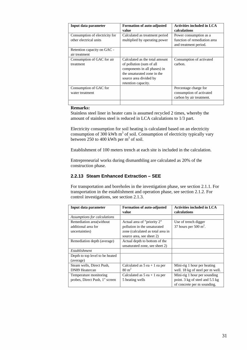
31
Input data parameter Formation of auto-adjusted
value
Activities included in LCA
calculations
Consumption of electricity for
other electrical units
Calculated as treatment period
multiplied by operating power
Power consumption as a
function of remediation area and treatment period.
Retention capacity on GAC -air treatment
Consumption of GAC for air treatment
Calculated as the total amount of pollution (sum of all components in all phases) in
the unsaturated zone in the source area divided by
retention capacity.
Consumption of activated carbon.
Consumption of GAC for
water treatment
Percentage charge for
consumption of activated carbon by air treatment.
Remarks:Stainless steel liner in heater cans is assumed recycled 2 times, whereby the amount of stainless steel is reduced in LCA calculations to 1/3 part.
Electricity consumption for soil heating is calculated based on an electricity consumption of 300 kWh m3 of soil. Consumption of electricity typically vary between 250 to 400 kWh per m3 of soil.
Establishment of 100 meters trench at each site is included in the calculation.
Entrepreneurial works during dismanthling are calculated as 20% of the construction phase.
2.2.13 Steam Enhanced Extraction – SEE
For transportation and boreholes in the investigation phase, see section 2.1.1. For transportation in the establishment and operation phase, see section 2.1.2. For control investigations, see section 2.1.3.
Input data parameter Formation of auto-adjusted value
Activities included in LCA calculations
Assumptions for calculations
Remediation area(without
additional area for uncertainties)
Actual area of ”priority 2”
pollution in the unsaturated zone (calculated as total area in
source area, see sheet 2)
Use of trench digger
37 hours per 500 m2.
Remediation depth (average) Actual depth to bottom of the
unsaturated zone, see sheet 2)
Establishment
Depth to top level to be heated(average)
Steam wells, Direct Push, DN89 Heatercan
Calculated as 5 ea + 1 ea per 80 m2
Mini-rig 1 hour per heating well. 18 kg of steel per m well.
Temperature monitoring probes, Direct Push, 1" screen
Calculated as 5 ea + 1 ea per 5 heating wells
Mini-rig 1 hour per sounding point. 3 kg of steel and 5.5 kg of concrete per m sounding.
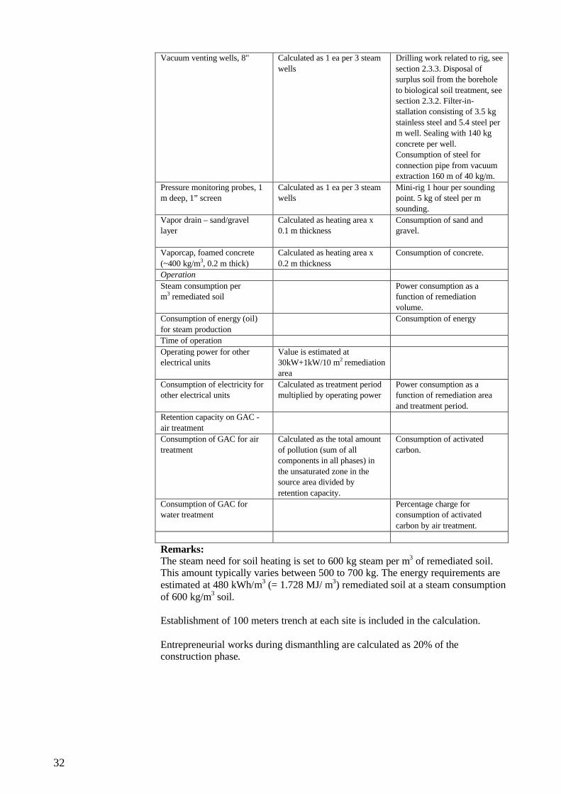
32
Vacuum venting wells, 8" Calculated as 1 ea per 3 steam
wells
Drilling work related to rig, see
section 2.3.3. Disposal of surplus soil from the borehole
to biological soil treatment, see section 2.3.2. Filter-in-stallation consisting of 3.5 kg
stainless steel and 5.4 steel per m well. Sealing with 140 kg
concrete per well. Consumption of steel for
connection pipe from vacuum extraction 160 m of 40 kg/m.
Pressure monitoring probes, 1 m deep, 1” screen
Calculated as 1 ea per 3 steam wells
Mini-rig 1 hour per sounding point. 5 kg of steel per m sounding.
Vapor drain – sand/gravel layer
Calculated as heating area x 0.1 m thickness
Consumption of sand and gravel.
Vaporcap, foamed concrete
(~400 kg/m3, 0.2 m thick)
Calculated as heating area x
0.2 m thickness
Consumption of concrete.
Operation
Steam consumption per m3 remediated soil
Power consumption as a function of remediation
volume.
Consumption of energy (oil)
for steam production
Consumption of energy
Time of operation
Operating power for other electrical units
Value is estimated at 30kW+1kW/10 m2 remediationarea
Consumption of electricity for other electrical units
Calculated as treatment period multiplied by operating power
Power consumption as a function of remediation area
and treatment period.
Retention capacity on GAC -
air treatment
Consumption of GAC for air
treatment
Calculated as the total amount
of pollution (sum of all components in all phases) in
the unsaturated zone in the source area divided by
retention capacity.
Consumption of activated
carbon.
Consumption of GAC for water treatment
Percentage charge for consumption of activated
carbon by air treatment.
Remarks:The steam need for soil heating is set to 600 kg steam per m3 of remediated soil. This amount typically varies between 500 to 700 kg. The energy requirements are estimated at 480 kWh/m3 (= 1.728 MJ/ m3) remediated soil at a steam consumption of 600 kg/m3 soil.
Establishment of 100 meters trench at each site is included in the calculation.
Entrepreneurial works during dismanthling are calculated as 20% of the construction phase.
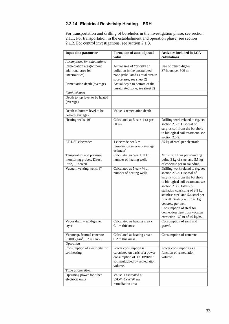
33
2.2.14 Electrical Resistivity Heating – ERH
For transportation and drilling of boreholes in the investigation phase, see section 2.1.1. For transportation in the establishment and operation phase, see section 2.1.2. For control investigations, see section 2.1.3.
Input data parameter Formation of auto-adjusted value
Activities included in LCA calculations
Assumptions for calculations
Remediation area(without
additional area for uncertainties)
Actual area of ”priority 1”
pollution in the unsaturated zone (calculated as total area in
source area, see sheet 2)
Use of trench digger
37 hours per 500 m2.
Remediation depth (average) Actual depth to bottom of the unsaturated zone, see sheet 2)
Establishment
Depth to top level to be heated (average)
Depth to bottom level to be heated (average)
Value is remediation depth
Heating wells, 10" Calculated as 5 ea + 1 ea per 30 m2
Drilling work related to rig, see section 2.3.3. Disposal of
surplus soil from the borehole to biological soil treatment, see
section 2.3.2.
ET-DSP electrodes 1 electrode per 3 m
remediation interval (average estimate)
35 kg of steel per electrode
Temperature and pressure
monitoring probes, Direct Push, 1" screen
Calculated as 5 ea + 1/3 of
number of heating wells
Mini-rig 1 hour per sounding
point. 3 kg of steel and 5.5 kg of concrete per m sounding.
Vacuum venting wells, 8" Calculated as 5 ea + ¼ of number of heating wells
Drilling work related to rig, see section 2.3.3. Disposal of
surplus soil from the borehole to biological soil treatment, see
section 2.3.2. Filter-in-stallation consisting of 3.5 kg stainless steel and 5.4 steel per
m well. Sealing with 140 kg concrete per well.
Consumption of steel for connection pipe from vacuum
extraction 160 m of 40 kg/m.
Vapor drain – sand/gravel
layer
Calculated as heating area x
0.1 m thickness
Consumption of sand and
gravel.
Vaporcap, foamed concrete (~400 kg/m3, 0.2 m thick)
Calculated as heating area x 0.2 m thickness
Consumption of concrete.
Operation
Consumption of electricity for soil heating
Power consumption is calculated on basis of a power
consumption of 300 kWh/m3 soil multiplied by remediation
volume.
Power consumption as a function of remediation
volume.
Time of operation
Operating power for other electrical units
Value is estimated at 35kW+1kW/20 m2
remediation area
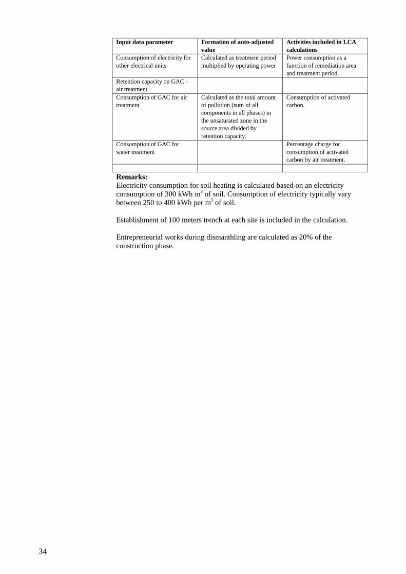
34
Input data parameter Formation of auto-adjusted
value
Activities included in LCA
calculations
Consumption of electricity for
other electrical units
Calculated as treatment period
multiplied by operating power
Power consumption as a
function of remediation area and treatment period.
Retention capacity on GAC -air treatment
Consumption of GAC for air treatment
Calculated as the total amount of pollution (sum of all components in all phases) in
the unsaturated zone in the source area divided by
retention capacity.
Consumption of activated carbon.
Consumption of GAC for
water treatment
Percentage charge for
consumption of activated carbon by air treatment.
Remarks:Electricity consumption for soil heating is calculated based on an electricity consumption of 300 kWh m3 of soil. Consumption of electricity typically vary between 250 to 400 kWh per m3 of soil.
Establishment of 100 meters trench at each site is included in the calculation.
Entrepreneurial works during dismanthling are calculated as 20% of the construction phase.
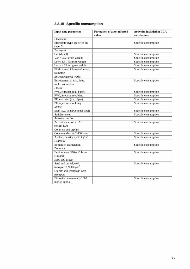
35
2.2.15 Specific consumption
Input data parameter Formation of auto-adjusted value
Activities included in LCA calculations
Electricity
Electricity (type specified on
sheet 5)
Specific consumption
Transport
Car (diesel) Specific consumption
Van < 3.5 t gross weight Specific consumption
Lorry 3.5-7.5t gross weight Specific consumption
Lorry > 32 ton gross weight Specific consumption
Flight travel, kilometer/person,roundtrip
Specific consumption
Entrepreneurial works
Entrepreneurial machines,
fuel consumption
Specific consumption
Plastic
PVC, extruded (e.g. pipes) Specific consumption
PVC, injection moulding Specific consumption
PE, extruded (e.g. pipes) Specific consumption
PE, injection moulding Specific consumption
Metals
Steel (e.g. constructional steel) Specific consumption
Stainless steel Specific consumption
Activated carbon
Activated carbon - GAC(origin EU)
Specific consumption
Concrete and asphalt
Concrete, density 2,400 kg/m3 Specific consumption
Asphalt, density 2,250 kg/m3 Specific consumption
Bentonite
Bentonite, extracted in Denmark
Specific consumption
Bentonite as "Mikolit" from Holland
Specific consumption
Sand and gravel
Sand and gravel, excl.
transport, 1,900 kg/m3Specific consumption
Off-site soil treatment, excl.
transport
Biological treatment (~1000 mg/kg light oil)
Specific consumption
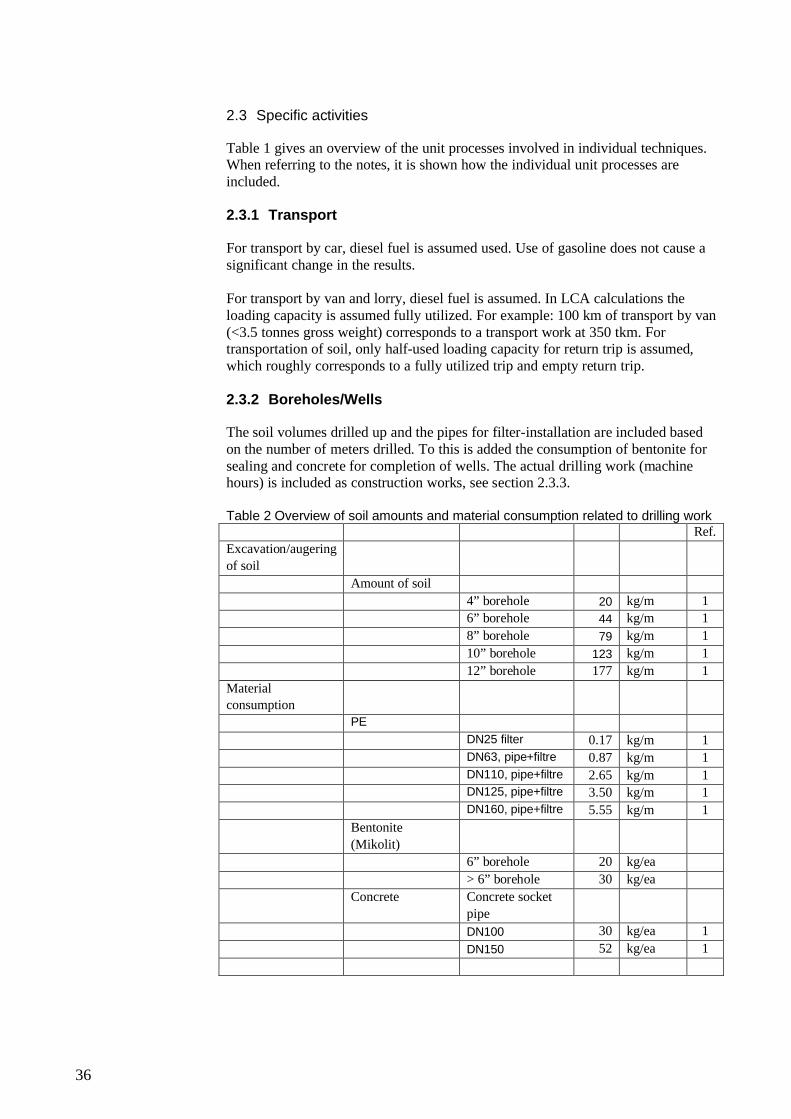
36
2.3 Specific activities
Table 1 gives an overview of the unit processes involved in individual techniques. When referring to the notes, it is shown how the individual unit processes are included.
2.3.1 Transport
For transport by car, diesel fuel is assumed used. Use of gasoline does not cause a significant change in the results.
For transport by van and lorry, diesel fuel is assumed. In LCA calculations the loading capacity is assumed fully utilized. For example: 100 km of transport by van (<3.5 tonnes gross weight) corresponds to a transport work at 350 tkm. For transportation of soil, only half-used loading capacity for return trip is assumed, which roughly corresponds to a fully utilized trip and empty return trip.
2.3.2 Boreholes/Wells
The soil volumes drilled up and the pipes for filter-installation are included based on the number of meters drilled. To this is added the consumption of bentonite for sealing and concrete for completion of wells. The actual drilling work (machine hours) is included as construction works, see section 2.3.3.
Table 2 Overview of soil amounts and material consumption related to drilling workRef.
Excavation/augering
of soil
Amount of soil
4” borehole 20 kg/m 1
6” borehole 44 kg/m 1
8” borehole 79 kg/m 1
10” borehole 123 kg/m 1
12” borehole 177 kg/m 1
Materialconsumption
PE
DN25 filter 0.17 kg/m 1DN63, pipe+filtre 0.87 kg/m 1DN110, pipe+filtre 2.65 kg/m 1DN125, pipe+filtre 3.50 kg/m 1DN160, pipe+filtre 5.55 kg/m 1
Bentonite
(Mikolit)
6” borehole 20 kg/ea
> 6” borehole 30 kg/ea
Concrete Concrete socket
pipe
DN100 30 kg/ea 1
DN150 52 kg/ea 1
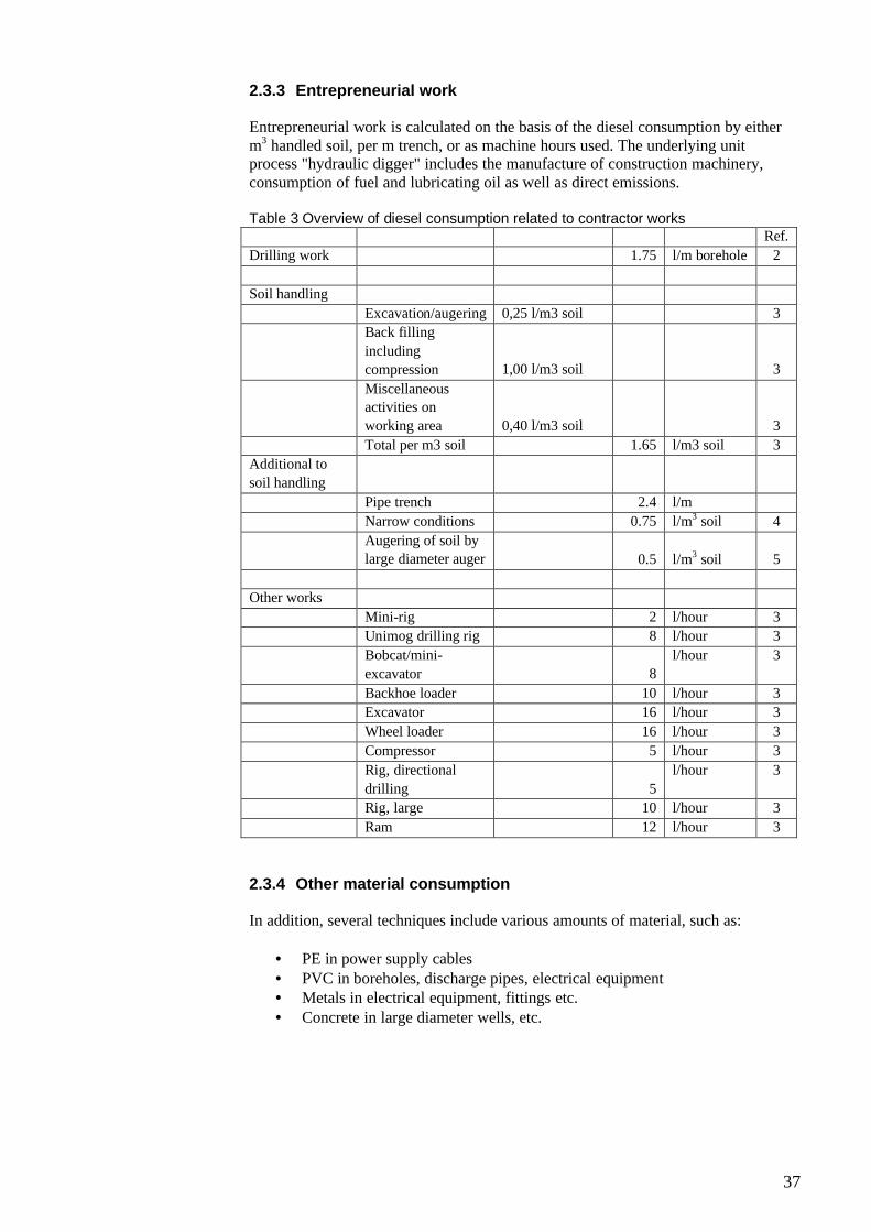
37
2.3.3 Entrepreneurial work
Entrepreneurial work is calculated on the basis of the diesel consumption by either m3 handled soil, per m trench, or as machine hours used. The underlying unit process "hydraulic digger" includes the manufacture of construction machinery,consumption of fuel and lubricating oil as well as direct emissions.
Table 3 Overview of diesel consumption related to contractor worksRef.
Drilling work 1.75 l/m borehole 2
Soil handling
Excavation/augering 0,25 l/m3 soil 3
Back filling
including
compression 1,00 l/m3 soil 3
Miscellaneousactivities on
working area 0,40 l/m3 soil 3
Total per m3 soil 1.65 l/m3 soil 3
Additional to
soil handling
Pipe trench 2.4 l/m
Narrow conditions 0.75 l/m3 soil 4
Augering of soil by large diameter auger 0.5 l/m3 soil 5
Other works
Mini-rig 2 l/hour 3
Unimog drilling rig 8 l/hour 3
Bobcat/mini-
excavator 8
l/hour 3
Backhoe loader 10 l/hour 3
Excavator 16 l/hour 3
Wheel loader 16 l/hour 3
Compressor 5 l/hour 3
Rig, directional
drilling 5
l/hour 3
Rig, large 10 l/hour 3
Ram 12 l/hour 3
2.3.4 Other material consumption
In addition, several techniques include various amounts of material, such as:
• PE in power supply cables• PVC in boreholes, discharge pipes, electrical equipment• Metals in electrical equipment, fittings etc. • Concrete in large diameter wells, etc.
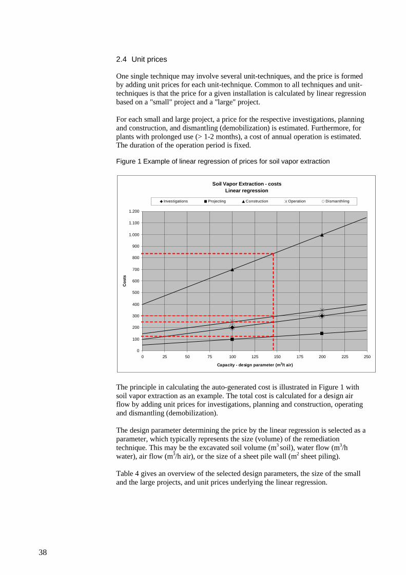
38
2.4 Unit prices
One single technique may involve several unit-techniques, and the price is formed by adding unit prices for each unit-technique. Common to all techniques and unit-techniques is that the price for a given installation is calculated by linear regression based on a "small" project and a "large" project.
For each small and large project, a price for the respective investigations, planning and construction, and dismantling (demobilization) is estimated. Furthermore, for plants with prolonged use (> 1-2 months), a cost of annual operation is estimated. The duration of the operation period is fixed.
Figure 1 Example of linear regression of prices for soil vapor extraction
Soil Vapor Extraction - costs
Linear regression
0
100
200
300
400
500
600
700
800
900
1.000
1.100
1.200
0 25 50 75 100 125 150 175 200 225 250
Capacity - design parameter (m3/t air)
Co
sts
Investigations Projecting Construction Operation Dismanthling
The principle in calculating the auto-generated cost is illustrated in Figure 1 with soil vapor extraction as an example. The total cost is calculated for a design airflow by adding unit prices for investigations, planning and construction, operating and dismantling (demobilization).
The design parameter determining the price by the linear regression is selected as a parameter, which typically represents the size (volume) of the remediation technique. This may be the excavated soil volume (m3 soil), water flow (m3/h water), air flow (m3/h air), or the size of a sheet pile wall (m2 sheet piling).
Table 4 gives an overview of the selected design parameters, the size of the small and the large projects, and unit prices underlying the linear regression.
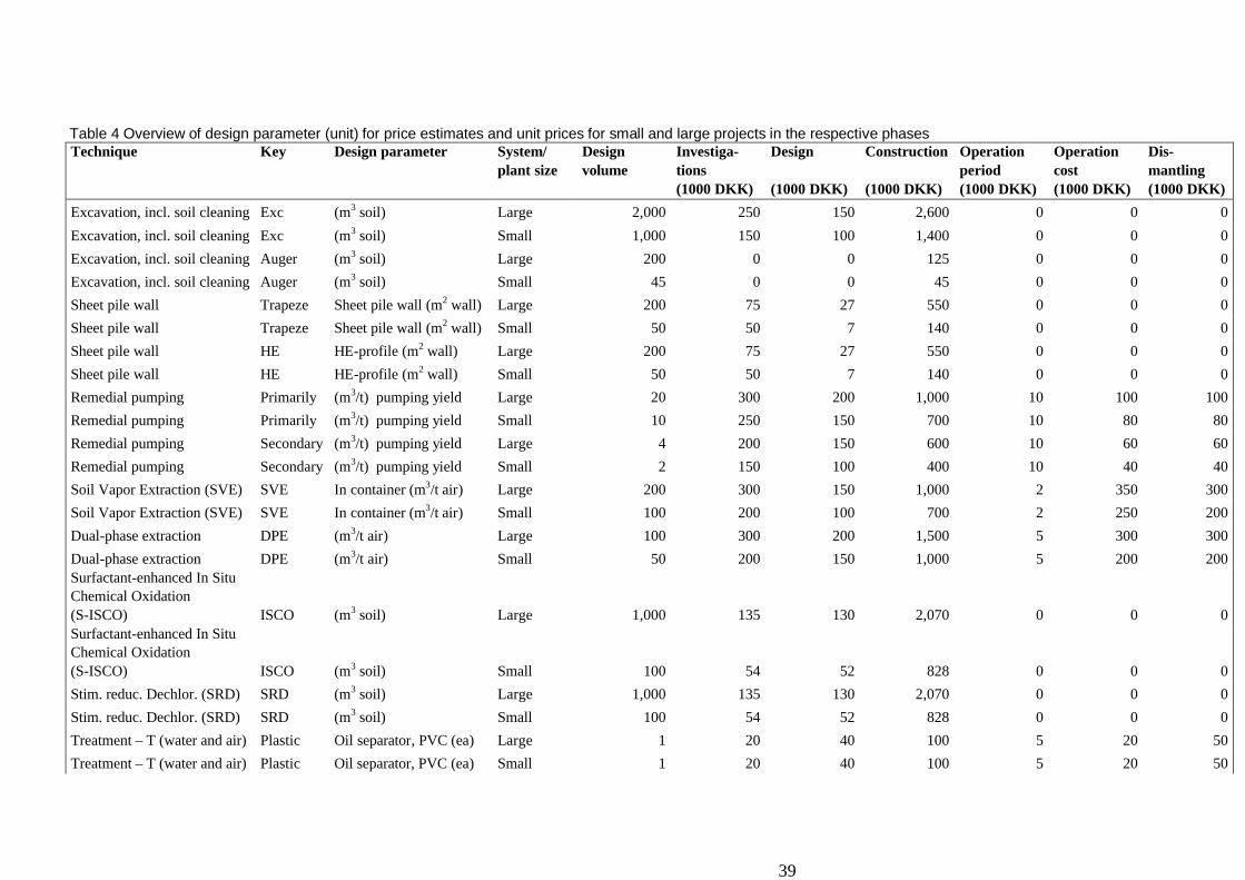
39
Table 4 Overview of design parameter (unit) for price estimates and unit prices for small and large projects in the respective phasesTechnique Key Design parameter System/
plant size
Design
volume
Investiga-
tions
(1000 DKK)
Design
(1000 DKK)
Construction
(1000 DKK)
Operation
period
(1000 DKK)
Operation
cost
(1000 DKK)
Dis-
mantling
(1000 DKK)
Excavation, incl. soil cleaning Exc (m3 soil) Large 2,000 250 150 2,600 0 0 0
Excavation, incl. soil cleaning Exc (m3 soil) Small 1,000 150 100 1,400 0 0 0
Excavation, incl. soil cleaning Auger (m3 soil) Large 200 0 0 125 0 0 0
Excavation, incl. soil cleaning Auger (m3 soil) Small 45 0 0 45 0 0 0
Sheet pile wall Trapeze Sheet pile wall (m2 wall) Large 200 75 27 550 0 0 0
Sheet pile wall Trapeze Sheet pile wall (m2 wall) Small 50 50 7 140 0 0 0
Sheet pile wall HE HE-profile (m2 wall) Large 200 75 27 550 0 0 0
Sheet pile wall HE HE-profile (m2 wall) Small 50 50 7 140 0 0 0
Remedial pumping Primarily (m3/t) pumping yield Large 20 300 200 1,000 10 100 100
Remedial pumping Primarily (m3/t) pumping yield Small 10 250 150 700 10 80 80
Remedial pumping Secondary (m3/t) pumping yield Large 4 200 150 600 10 60 60
Remedial pumping Secondary (m3/t) pumping yield Small 2 150 100 400 10 40 40
Soil Vapor Extraction (SVE) SVE In container (m3/t air) Large 200 300 150 1,000 2 350 300
Soil Vapor Extraction (SVE) SVE In container (m3/t air) Small 100 200 100 700 2 250 200
Dual-phase extraction DPE (m3/t air) Large 100 300 200 1,500 5 300 300
Dual-phase extraction DPE (m3/t air) Small 50 200 150 1,000 5 200 200
Surfactant-enhanced In Situ Chemical Oxidation
(S-ISCO) ISCO (m3 soil) Large 1,000 135 130 2,070 0 0 0
Surfactant-enhanced In Situ Chemical Oxidation
(S-ISCO) ISCO (m3 soil) Small 100 54 52 828 0 0 0
Stim. reduc. Dechlor. (SRD) SRD (m3 soil) Large 1,000 135 130 2,070 0 0 0
Stim. reduc. Dechlor. (SRD) SRD (m3 soil) Small 100 54 52 828 0 0 0
Treatment – T (water and air) Plastic Oil separator, PVC (ea) Large 1 20 40 100 5 20 50
Treatment – T (water and air) Plastic Oil separator, PVC (ea) Small 1 20 40 100 5 20 50
40
Technique Key Design parameter System/
plant size
Design
volume
Investiga-
tions
(1000 DKK)
Design
(1000 DKK)
Construction
(1000 DKK)
Operation
period
(1000 DKK)
Operation
cost
(1000 DKK)
Dis-
mantling
(1000 DKK)
Treatment – T (water and air) Concrete
Oil separator, concrete(ea) Large 1 20 40 100 5 20 50
Treatment – T (water and air) Concrete
Oil separator, concrete
(ea) Small 1 20 40 100 5 20 50
Treatment – T (water and air) cont-water Water, container Large 20 150 150 3,000 5 150 300
Treatment – T (water and air) cont-water Water, container Small 10 100 100 2,000 5 100 200
Treatment – T (water and air)
building-
water Water, building Large 20 150 250 5,000 5 150 600
Treatment – T (water and air)
building-
water Water, building Small 10 100 200 3,500 5 100 400
Treatment – T (water and air) Aerated Aerated water (m3/t) Large 20 50 75 300 5 300 100
Treatment – T (water and air) Aerated Aerated water (m3/t) Small 10 50 50 200 5 200 75
Treatment – T (water and air) Active Air flow, active (m3/t) Large 200 25 75 400 5 250 75
Treatment – T (water and air) Active Air flow, active (m3/t) Small 100 25 50 200 5 150 50
Treatment – T (water and air) Passive Air flow, passive (m3/t) Large 20 50 75 200 5 40 60
Treatment – T (water and air) Passive Air flow, passive (m3/t) Small 10 25 50 150 5 30 40
Soilmixing + microscale ZVI ZVI (m3 soil) Large 1,000 315 140 1,895 0 0 0
Soilmixing + microscale ZVI ZVI (m3 soil) Small 100 126 56 758 0 0 0
Natural attenuation (NA) NA (m3 soil) Large 10,000 200 60 0 5 50 50
Natural attenuation (NA) NA (m3 soil) Small 1,000 100 40 0 5 30 20
Steam Enhanced Extraction
(SEE) SEE (m3 soil) Large 11,000 850 1,200 13,126 0 0 0
Steam Enhanced Extraction (SEE) SEE (m3 soil) Small 2,000 500 800 5,028 0 0 0Passive Soil Vapor Extraction
(PSVE) PSVE (m3/t) Large 20 250 100 800 10 40 200
Passive Soil (PSVE) PSVE (m3/t) Small 10 200 80 500 10 30 150
In Situ Thermal Desorption (ISTD) ISTD (m3 soil) Large 11,000 850 1,200 17,133 0 0 0
41
Technique Key Design parameter System/
plant size
Design
volume
Investiga-
tions
(1000 DKK)
Design
(1000 DKK)
Construction
(1000 DKK)
Operation
period
(1000 DKK)
Operation
cost
(1000 DKK)
Dis-
mantling
(1000 DKK)
In Situ Thermal Desorption (ISTD) ISTD (m3 soil) Small 2,000 500 800 6,228 0 0 0Electrical Resistivity Heating
(ERH) ERH (m3 soil) Large 11,000 850 692 17,316 0 0 0Electrical Resistivity Heating
(ERH) ERH (m3 soil) Small 2,000 500 660 6,968 0 0 0
The unit prices for each technique are partly based on NIRAS’ knowledge on standard prices and partly on contractor’s informations.
REFERENCES
1. Banestyrelsen rådgivning; HOH Vand og Miljø A/S; NIRAS Rådgivende ingeniører og planlæggere A/S; Revisorsamvirket / Pannell Kerr Forster (2000): Miljørigtig oprensning af forurenede grunde. EU LIFE Project no. 96ENV/DK/0016. Copenhagen, Denmark. Prepared for Banestyrelsen, DSB and Miljøstyrelsen.
2. Glipstrup A/S3. Arkil A/S by Kim R. Jensen4. Arkil A/S by Claus Lundgaard5. Arkil A/S by Jon Boi Pedersen

42
43
3 Unit Processes
The life cycle inventory data for "cradle to gate" unit processes used in RemS are mainly based on the ecoinvent database version 2.0 (Frischknecht et al. 2007).
Ecoinvent’s unit processes for finished goods (steel, plastics, etc.) include environmental exchanges (resource consumption and emissions) related to the material and production phase of a product, i.e. extracting raw materials, production and transportation, but not the use phase and the final disposal of the produced product.
The unit processes in ecoinvent furthermore involve elements of infrastructure such as construction of a plant, a vehicle, etc., used for production or transportation of goods. A portion of the infrastructure environmental impacts is allotted the finished product in a ratio that is based on the estimated life time of the infrastructure.
The production processes in ecoinvent usually represent average European production conditions. Electricity generation is, however, available to all European countries. Table 1-11 list the applied ecoinvent unit processes and their temporal and geographic coverage. Some of the used unit processes are developed by combining a number ecoinvent processes, for example by adding extra transport or input of energy or material consumption.
The LCA software SimaPro version 7.1.8 is used for modelling the life cycle inventories and to calculate life cycle impacts related to each of the processes is listed in the Appendix.
Electricity productionElectricity consumption is often a significant contributor to environmental impacts in a life cycle assessment. The production technology that is chosen to represent the electricity consumption is therefore of great importance for the outcome of the life cycle assessment.
In RemS, it is possible to switch between power compositions representing a number of different countries or regions: DK, NO, SE, UCTE, and EU27. In addition, you can select specific production technologies such as natural gas, coal, and wind power. In table 1A-1C, is an overview of electricity production processes.
To represent the electricity used directly for remediation activities (on site or off site), the average electricity production in the country of the remediation can beused as a starting point. This can be complemented with a sensitivity scenario,including the marginal electricity production technology. The marginal electricity production technology is in the short term also the one that can immediately increase production if demand rises.
According to Weidema (2003), the marginal electricity supply in Denmark will in the short term be based on coal and in the rest of Europe be based on gas. For long term projects (over 10-20 years), the proportion of wind energy is expected to increase. Wind processes, representing production of wind power through land-based windmills as well as offshore windmills, is therefore included in the toolthereby allowing sensitivity analyses of wind energy as a power source.
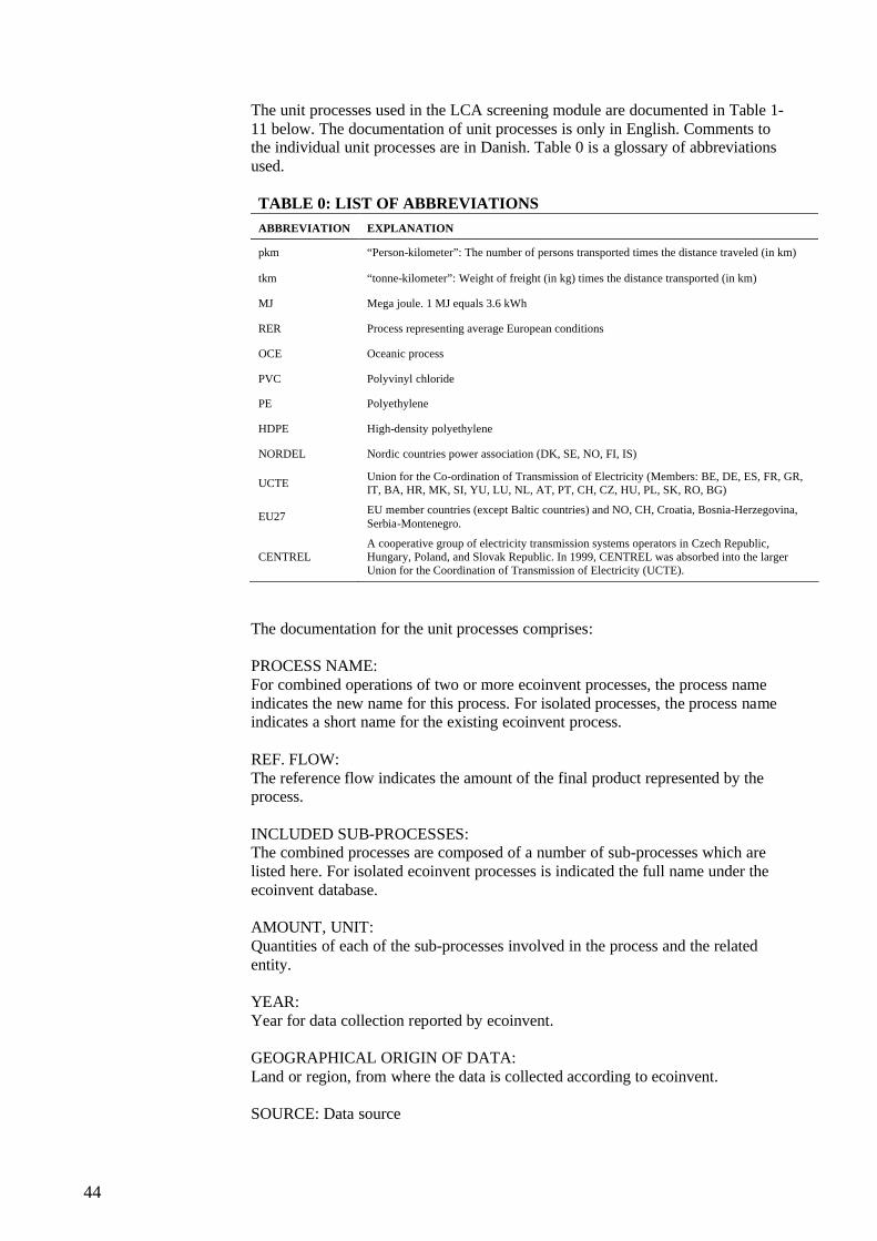
44
The unit processes used in the LCA screening module are documented in Table 1-11 below. The documentation of unit processes is only in English. Comments to the individual unit processes are in Danish. Table 0 is a glossary of abbreviations used.
TABLE 0: LIST OF ABBREVIATIONS
ABBREVIATION EXPLANATION
pkm “Person-kilometer”: The number of persons transported times the distance traveled (in km)
tkm “tonne-kilometer”: Weight of freight (in kg) times the distance transported (in km)
MJ Mega joule. 1 MJ equals 3.6 kWh
RER Process representing average European conditions
OCE Oceanic process
PVC Polyvinyl chloride
PE Polyethylene
HDPE High-density polyethylene
NORDEL Nordic countries power association (DK, SE, NO, FI, IS)
UCTEUnion for the Co-ordination of Transmission of Electricity (Members: BE, DE, ES, FR, GR, IT, BA, HR, MK, SI, YU, LU, NL, AT, PT, CH, CZ, HU, PL, SK, RO, BG)
EU27EU member countries (except Baltic countries) and NO, CH, Croatia, Bosnia-Herzegovina, Serbia-Montenegro.
CENTRELA cooperative group of electricity transmission systems operators in Czech Republic, Hungary, Poland, and Slovak Republic. In 1999, CENTREL was absorbed into the larger Union for the Coordination of Transmission of Electricity (UCTE).
The documentation for the unit processes comprises:
PROCESS NAME:For combined operations of two or more ecoinvent processes, the process name indicates the new name for this process. For isolated processes, the process name indicates a short name for the existing ecoinvent process.
REF. FLOW:The reference flow indicates the amount of the final product represented by the process.
INCLUDED SUB-PROCESSES: The combined processes are composed of a number of sub-processes which arelisted here. For isolated ecoinvent processes is indicated the full name under the ecoinvent database.
AMOUNT, UNIT: Quantities of each of the sub-processes involved in the process and the related entity.
YEAR: Year for data collection reported by ecoinvent.
GEOGRAPHICAL ORIGIN OF DATA: Land or region, from where the data is collected according to ecoinvent.
SOURCE: Data source
45
TABLE 1A: ELECTRICITY – Consumer mixes
PROCESS NAMEREF. FLOW INCLUDED SUBPROCESSES AMOUNT UNIT
YEAR 1
GEOGRAPHICAL ORIGIN OF DATA SOURCE
Electricity DK 1 MJ Electricity, low voltage, at grid/DK 1 MJ2004-2005
Denmark ecoinvent
Electricity DK (alloc.)
1 MJ Electricity, low voltage, at grid/DK 0.828 MJ2004-2005
Denmark ecoinvent
Electricity SE 1 MJ Electricity, low voltage, at grid/SE 1 MJ2004-2005
Sweden ecoinvent
Electricity NO 1 MJ Electricity, low voltage, at grid/NO 1 MJ2004-2005
Norway ecoinvent
Electricity UCTE 1 MJElectricity, low voltage, production UCTE, at grid/UCTE
1 MJ2004-2005
Continental Europe ecoinvent
Electricity EU27 1 MJElectricity, low voltage, production RER, at grid/RER
1 MJ2004-2005
EU27 ecoinvent
General description of processes:
All electricity processes above represent electricity at low voltage delivered to the consumer, i.e. electricity losses during transformation and distribution to the consumer is accounted for. Infrastructure is included (network, power plant etc.).
DK, SE and NO electricity represents average Danish, Swedish and Norwegian electricity production respectively including imports (see composition of production technologies for each country in Table 1C.
Electricity DK (alloc.) is equal to 'Electricity DK', but 17.2% of the environmental impacts are allocated to district heating which is a co-product of electricity production. The allocation is done based on the energy quality (exergy) in the produced electricity and heat respectively .The allocation method is described in Energinet.dk (2008)
Electricity UCTE represents the average electricity production in the UCTE member countries, see Table 0.
Electricity EU27 represents the average electricity production in the EU member countries (except Baltic countries) and NO, CH, Croatia, Bosnia-Herzegovina, Serbia-Montenegro.
1 Refers to age of the inventory data in ecoinvent
TABLE 1B: ELECTRICITY – Single production technologies
PROCESS NAMEREF. FLOW INCLUDED SUBPROCESSES AMOUNT UNIT
YEAR 1
GEOGRAPHICAL ORIGIN OF DATA SOURCE
Electricity, coal (marginal)
1 MJElectricity, hard coal, low voltage, at grid/NORDEL
1 MJ 2000 Nordic countries ecoinvent
Electricity, natural gas (marginal)
1 MJElectricity, natural gas, low voltage, at grid/NORDEL
1 MJ 2000 Nordic countries ecoinvent
Electricity, wind power, off shore, 2MW
1 MJElectricity, wind power 2MW, offshore, low voltage at grid/OCE
1 MJ 2002 Europe ecoinvent
Electricity, wind power, on shore, 800 kW
1 MJElectricity, wind power 800 kW, offshore, low voltage at grid/OCE
1 MJ 2002 Europe ecoinvent
General description of processes:Electricity production from coal and natural gas represents possible marginal production technologies for electricity production in Denmark. The ecoinvent processes do not include energy loss and emissions during transformation and distribution of electricity, but this has been added assuming the same loss as for average Danish electricity. Infrastructure is included (network, power plant etc.)
The ecoinvent processes for electricity production from wind energy do not include energy loss and emissions during transformation and distribution of electricity, but this has been added assuming the same loss as for average Danish electricity. Infrastructure (network, wind power plant etc.) and the operation of the wind power plant with the necessary change of gear oil is included. The lifetime of moving and fixed parts is assumed to be 20 resp. 40 years.
1 Refers to age of the inventory data in ecoinvent
46
TABLE 1C: ELECTRICITY – Consumer mix composition
COMPOSITION OF ELECTRICITY SOURCES (%)
Denmark (DK) Norway (NO) Sweden (SE)
Hard coal 38.4 0.03 0.61
Peat - - 0.41
Oil 3.4 0.01 1.17
Natural gas 20.5 0.28 0.45
Industrial gas 0.0 0.04 0.49
Hydropower 0.1 86.86 36.62
Nuclear - - 46.09
Wind power 14.4 0.24 0.55
Biomass 3.8 0.23 3.97
Biogas 0.5 - 0.06
Import, DE 7.4 - 0.87
Import, NO 3.2 - 1.39
Import, SE 8.3 8.97 -
Import DK - 3.06 1.52
Import, FI - 0.13 4.34Import, CENTREL - 0.15 -
Import, PL - - 1.46
Database: ecoinvent Version 2.0
47
TABLE 2: HEATING
PROCESS NAMEREF. FLOW INCLUDED SUBPROCESSES AMOUNT UNIT
YEAR 1
GEOGRAPHICAL ORIGIN OF DATA SOURCE
Heat boiler, 100kW 1 MJHeat, light fuel oil, at boiler 100kW, non-modulating/CH
1 MJ 2000 Switzerland Ecoinvent
General description of process:Heating of water using a non-modulating, non-condensing boiler with an efficiency of 94%. The material for the heat boiler is not included, but the full life cycle for the fuel oil is included.
1 Refers to age of the inventory data in ecoinvent
TABLE 3: TRANSPORT
PROCESS NAMEREF. FLOW INCLUDED SUBPROCESSES AMOUNT UNIT
YEAR 1
GEOGRAPHICAL ORIGIN OF DATA SOURCE
Car, diesel 1 pkmTransport, car, diesel, EURO4/CH
1 pkm2004-2005
Switzerland Ecoinvent
Van < 3.5 t 1 tkm Transport, van <3.5t/RER U 1 tkm2004-2005
Europe Ecoinvent
Lorry 3.5-7.5 t 1 tkmTransport, lorry 3.5-7.5t, EURO3/RER U
1 tkm2004-2005
Europe Ecoinvent
Lorry > 32 t 1 tkmTransport, lorry >32t, EURO3/RER
1 tkm2004-2005
Europe Ecoinvent
Aircraft, passenger 1 pkmTransport, aircraft, passenger/RER
1 pkm 2002 Europe Ecoinvent
General description of processes:The transport processes include direct transport emissions as well as manufacturing of the vehicle/aeroplane and fuel. Furthermore it includes infrastructure (airport- and road construction)
The 'Aircraft, passenger' process is a combined process assuming 75% intereuropean and 25% intercontinental flights.
1 Refers to age of the inventory data used in ecoinvent
TABLE 4: ENTREPRENEURIAL WORKS
PROCESS NAMEREF. FLOW INCLUDED SUBPROCESSES AMOUNT UNIT
YEAR 1
GEOGRAPHICAL ORIGIN OF DATA SOURCE
Hydraulic digger1 L diesel
Excavation, hydraulic digger, low sulphur diesel/RER
7.63 m3 2000 Europe Ecoinvent
General description of process:The process includes direct emissions as well as manufacturing of the entrepreneurial machine and the consumption of fuel and lubricating oil. The reference flow for the original ecoinvent process is excavation of 1 m3 soil. In the above process the reference flow has been changed to 1 l diesel used by the machine.
1 Refers to age of the inventory data in ecoinvent
48
TABLE 5: PLASTICS
PROCESS NAMEREF. FLOW INCLUDED SUBPROCESSES AMOUNT UNIT YEAR 1
GEOGRAPHICAL ORIGIN OF DATA SOURCE
PVC, extruded, at regional storage
1 kgPolyvinylchloride, at regional storage/RER
1 kg2005-2007
Europe Ecoinvent
Extrusion, plastic pipes/RER 1 kg2005-2007
Europe Ecoinvent
Transport, lorry > 16t, fleet average/RER
0.1 tkm2004-2005
Europe Ecoinvent
Transport, freight, rail/RER 0.2 tkm1999-2004
Europe Ecoinvent
1 kgPolyvinylchloride, at regional storage/RER
1 kg2005-2007
Europe EcoinventPVC, injection moulding, at regional storage Injection moulding/RER 1 1 kg
2005-2007
Europe Ecoinvent
Transport, lorry > 16t, fleet average/RER
0.1 tkm2004-2005
Europe ecoinvent
Transport, freight, rail/RER 0.2 tkm1999-2004
Europe ecoinvent
PE, extruded, at regional storage
1 kgPolyethylene, HDPE, granulate, at plant/RER
1 kg2005-2007
Europe ecoinvent
Extrusion, plastic pipes/RER 1 kg2005-2007
Europe ecoinvent
Transport, lorry > 16t, fleet average/RER
0.1 tkm2004-2005
Europe ecoinvent
Transport, freight, rail/RER 0.2 tkm1999-2004
Europe ecoinvent
1 kgPolyethylene, HDPE, granulate, at plant/RER
1 kg2005-2007
Europe ecoinventPE, injection moulding, at regional storage Extrusion, plastic pipes/RER 1 kg
2005-2007
Europe ecoinvent
Transport, lorry > 16t, fleet average/RER
0.1 tkm2004-2005
Europe ecoinvent
Transport, freight, rail/RER 0.2 tkm1999-2004
Europe ecoinvent
General description of processes:The processes include raw material acquisition, plastic production and manufacturing to pipes or a moulded product. The processes also include transport from production place to regional storage (Denmark) using transportation distances as suggested in ecoinvent (Frischknecht et al., 2007).
1 Refers to age of the inventory data in ecoinvent
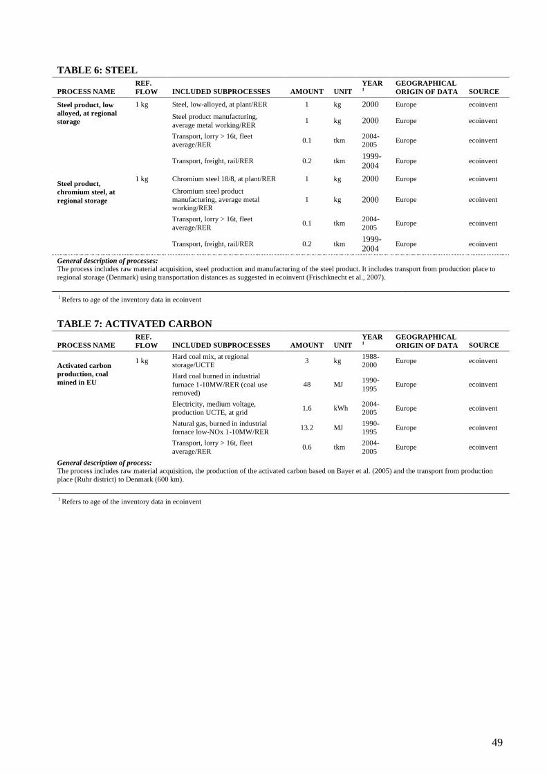
49
TABLE 6: STEEL
PROCESS NAMEREF. FLOW INCLUDED SUBPROCESSES AMOUNT UNIT
YEAR 1
GEOGRAPHICAL ORIGIN OF DATA SOURCE
1 kg Steel, low-alloyed, at plant/RER 1 kg 2000 Europe ecoinventSteel product, low alloyed, at regional storage
Steel product manufacturing, average metal working/RER
1 kg 2000 Europe ecoinvent
Transport, lorry > 16t, fleet average/RER
0.1 tkm2004-2005
Europe ecoinvent
Transport, freight, rail/RER 0.2 tkm1999-2004
Europe ecoinvent
1 kg Chromium steel 18/8, at plant/RER 1 kg 2000 Europe ecoinventSteel product, chromium steel, at regional storage
Chromium steel product manufacturing, average metal working/RER
1 kg 2000 Europe ecoinvent
Transport, lorry > 16t, fleet average/RER
0.1 tkm2004-2005
Europe ecoinvent
Transport, freight, rail/RER 0.2 tkm1999-2004
Europe ecoinvent
General description of processes:The process includes raw material acquisition, steel production and manufacturing of the steel product. It includes transport from production place to regional storage (Denmark) using transportation distances as suggested in ecoinvent (Frischknecht et al., 2007).
1 Refers to age of the inventory data in ecoinvent
TABLE 7: ACTIVATED CARBON
PROCESS NAMEREF. FLOW INCLUDED SUBPROCESSES AMOUNT UNIT
YEAR 1
GEOGRAPHICAL ORIGIN OF DATA SOURCE
1 kgHard coal mix, at regional storage/UCTE
3 kg1988-2000
Europe ecoinventActivated carbon production, coal mined in EU
Hard coal burned in industrial furnace 1-10MW/RER (coal use removed)
48 MJ1990-1995
Europe ecoinvent
Electricity, medium voltage, production UCTE, at grid
1.6 kWh2004-2005
Europe ecoinvent
Natural gas, burned in industrial fornace low-NOx 1-10MW/RER
13.2 MJ1990-1995
Europe ecoinvent
Transport, lorry > 16t, fleet average/RER
0.6 tkm2004-2005
Europe ecoinvent
General description of process:The process includes raw material acquisition, the production of the activated carbon based on Bayer et al. (2005) and the transport from production place (Ruhr district) to Denmark (600 km).
1 Refers to age of the inventory data in ecoinvent
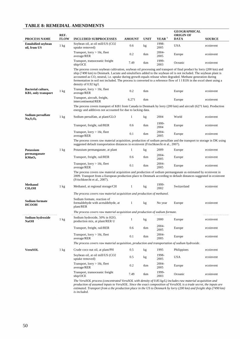
50
TABLE 8: REMEDIAL AMENDMENTS
PROCESS NAMEREF. FLOW INCLUDED SUBPROCESSES AMOUNT UNIT YEAR 1
GEOGRAPHICAL ORIGIN OF DATA SOURCE
Emulsified soybean oil, from US
1 kgSoybean oil, at oil mill/US (CO2 uptake removed)
0.6 kg1998-2005
USA ecoinvent
Transport, lorry > 16t, fleet average/RER
0.2 tkm2004-2005
Europe ecoinvent
Transport, transoceanic freight ship/OCE
7.49 tkm1999-2003
Oceanic ecoinvent
The process covers soybean cultivation, soybean oil processing and transport of final product by lorry (200 km) and ship (7490 km) to Denmark. Lactate and emulsifiers added to the soybean oil is not included. The soybean plant is accounted as CO2 neutral, i.e. uptake during growth equals release when degraded. Methane generation during fermentation in soil not included. The process is converted to a reference flow of 1 l EOS in the excel sheet using a density of 0.92 kg/l.
Bacterial culture, KB1, only transport
1 kgTransport, lorry > 16t, fleet average/RER
0.2 tkm Europe ecoinvent
Transport, aircraft, freight, intercontinental/RER
6.271 tkm Europe ecoinvent
The process covers transport of KB1 from Canada to Denmark by lorry (200 km) and aircraft (6271 km). Production energy and additives not accounted for due to lacking data.
Sodium persulfate Na2S2O8
1 kg Sodium persulfate, at plant/GLO 1 kg 2004 World ecoinvent
Transport, freight, rail/RER 0.6 tkm1999-2004
Europe ecoinvent
Transport, lorry > 16t, fleet average/RER
0.1 tkm2004-2005
Europe ecoinvent
The process covers raw material acquisition, production of sodium persulfate and the transport to storage in DK using suggested default transportation distances in ecoinvent (Frischknecht et al., 2007).
1 kg Potassium permanganate, at plant 1 kg 2009 Europe ecoinventPotassium permanganate KMnO4 Transport, freight, rail/RER 0.6 tkm
2004-2005
Europe ecoinvent
Transport, lorry > 16t, fleet average/RER
0.1 tkm2004-2005
Europe ecoinvent
The process covers raw material acquisition and production of sodium permanganate as estimated by ecoinvent in 2009. Transport from a European production place to Denmark according to default distances suggested in ecoinvent (Frischknecht et al., 2007).
MethanolCH3OH
1 kg Methanol, at regional storage/CH 1 kg1999-2002
Switzerland ecoinvent
The process covers raw material acquisition and production of methanol.
Sodium formateHCOOH
Sodium formate, reaction of formaldehyde with acetaldehyde, at plant/RER
1 kg No year Europe ecoinvent
The process covers raw material acquisition and production of sodium formate.
Sodium hydroxideNaOH
1 kgSodium hydroxide, 50% in H2O, production mix, at plant/RER U
1 kg 2000 Europe ecoinvent
Transport, freight, rail/RER 0.6 tkm2004-2005
Europe ecoinvent
Transport, lorry > 16t, fleet average/RER
0.1 tkm2004-2005
Europe ecoinvent
The process covers raw material acquisition, production and transportation of sodium hydroxide.
VeruSOL 1 kg Crude coco nut oil, at plant/PH 0.5 kg 1995 Philippines ecoinvent
Soybean oil, at oil mill/US (CO2 uptake removed)
0.5 kg1998-2005
USA ecoinvent
Transport, lorry > 16t, fleet average/RER
0.2 tkm2004-2005
Europe ecoinvent
Transport, transoceanic freight ship/OCE
7.49 tkm1999-2003
Oceanic ecoinvent
The VeruSOL process (concentrated VeruSOL with density of 0.85 kg/L) includes raw material acquisition and production of assumed inputs to VeruSOL. Since the exact composition of VeruSOL is a trade secret, the inputs are estimated. Transport from a the production place in the US to Denmark by lorry (200 km) and freight ship (7490 km) is included.
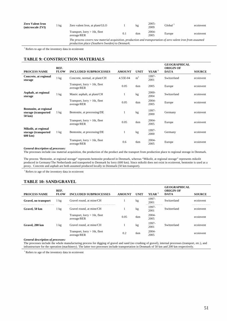
51
Zero Valent Iron (microscale ZVI)
1 kg Zero valent Iron, at plant/GLO 1 kg2005-2009
Global 2 ecoinvent
Transport, lorry > 16t, fleet average/RER
0.1 tkm2004-2005
Europe ecoinvent
The process covers raw material acquisition, production and transportation of zero valent iron from asuumed production place (Southern Sweden) to Denmark.
1 Refers to age of the inventory data in ecoinvent
TABLE 9: CONSTRUCTION MATERIALS
PROCESS NAMEREF. FLOW INCLUDED SUBPROCESSES AMOUNT UNIT YEAR 1
GEOGRAPHICAL ORIGIN OF DATA SOURCE
Concrete, at regional storage
1 kg Concrete, normal, at plant/CH 4.55E-04 m3 1997-2001
Switzerland ecoinvent
Transport, lorry > 16t, fleet average/RER
0.05 tkm 2005 Europe ecoinvent
Asphalt, at regional storage
1 kg Mastic asphalt, at plant/CH 1 kg2000-2004
Switzerland ecoinvent
Transport, lorry > 16t, fleet average/RER
0.05 tkm2004-2005
Europe ecoinvent
Bentonite, at regional storage (transported 50 km)
1 kg Bentonite, at processing/DE 1 kg1997-2000
Germany ecoinvent
Transport, lorry > 16t, fleet average/RER
0.05 tkm2004-2005
Europe ecoinvent
Mikolit, at regional storage (transported 600 km)
1 kg Bentonite, at processing/DE 1 kg1997-2000
Germany ecoinvent
Transport, lorry > 16t, fleet average/RER
0.6 tkm2004-2005
Europe ecoinvent
General description of processes:The processes include raw material acquisition, the production of the product and the transport from production place to regional storage in Denmark.
The process ‘Bentonite, at regional storage” represents bentonite produced in Denmark, whereas “Mikolit, at regional storage” represents mikolit produced in Germany/The Netherlands and transported to Denmark by lorry (600 km). Since mikolit does not exist in ecoinvent, bentonite is used as a proxy. Concrete and asphalt are both assumed produced locally in Denmark (50 km transport).
1 Refers to age of the inventory data in ecoinvent
TABLE 10: SAND/GRAVEL
PROCESS NAMEREF. FLOW INCLUDED SUBPROCESSES AMOUNT UNIT YEAR 1
GEOGRAPHICAL ORIGIN OF DATA SOURCE
Gravel, no transport 1 kg Gravel round, at mine/CH 1 kg1997-2001
Switzerland ecoinvent
Gravel, 50 km 1 kg Gravel round, at mine/CH 1 kg1997-2001
Switzerland ecoinvent
Transport, lorry > 16t, fleet average/RER
0.05 tkm2004-2005
ecoinvent
Gravel, 200 km 1 kg Gravel round, at mine/CH 1 kg1997-2001
Switzerland ecoinvent
Transport, lorry > 16t, fleet average/RER
0.2 tkm2004-2005
ecoinvent
General description of processes:The processes include the whole manufacturing process for digging of gravel and sand (no crushing of gravel), internal processes (transport, etc.), and infrastructure for the operation (machinery). The latter two processes include transportation in Denmark of 50 km and 200 km respectively.
1 Refers to age of the inventory data in ecoinvent
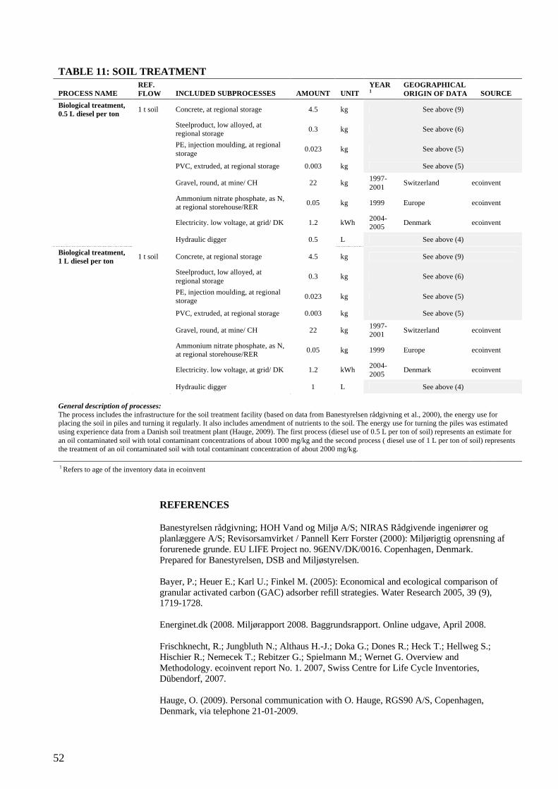
52
TABLE 11: SOIL TREATMENT
PROCESS NAMEREF. FLOW INCLUDED SUBPROCESSES AMOUNT UNIT
YEAR 1
GEOGRAPHICAL ORIGIN OF DATA SOURCE
Biological treatment, 0.5 L diesel per ton
1 t soil Concrete, at regional storage 4.5 kg See above (9)
Steelproduct, low alloyed, at regional storage
0.3 kg See above (6)
PE, injection moulding, at regional storage
0.023 kg See above (5)
PVC, extruded, at regional storage 0.003 kg See above (5)
Gravel, round, at mine/ CH 22 kg1997-2001
Switzerland ecoinvent
Ammonium nitrate phosphate, as N, at regional storehouse/RER
0.05 kg 1999 Europe ecoinvent
Electricity. low voltage, at grid/ DK 1.2 kWh2004-2005
Denmark ecoinvent
Hydraulic digger 0.5 L See above (4)
Biological treatment, 1 L diesel per ton
1 t soil Concrete, at regional storage 4.5 kg See above (9)
Steelproduct, low alloyed, at regional storage
0.3 kg See above (6)
PE, injection moulding, at regional storage
0.023 kg See above (5)
PVC, extruded, at regional storage 0.003 kg See above (5)
Gravel, round, at mine/ CH 22 kg1997-2001
Switzerland ecoinvent
Ammonium nitrate phosphate, as N, at regional storehouse/RER
0.05 kg 1999 Europe ecoinvent
Electricity. low voltage, at grid/ DK 1.2 kWh2004-2005
Denmark ecoinvent
Hydraulic digger 1 L See above (4)
General description of processes:The process includes the infrastructure for the soil treatment facility (based on data from Banestyrelsen rådgivning et al., 2000), the energy use for placing the soil in piles and turning it regularly. It also includes amendment of nutrients to the soil. The energy use for turning the piles was estimated using experience data from a Danish soil treatment plant (Hauge, 2009). The first process (diesel use of 0.5 L per ton of soil) represents an estimate for an oil contaminated soil with total contaminant concentrations of about 1000 mg/kg and the second process ( diesel use of 1 L per ton of soil) represents the treatment of an oil contaminated soil with total contaminant concentration of about 2000 mg/kg.
1 Refers to age of the inventory data in ecoinvent
REFERENCES
Banestyrelsen rådgivning; HOH Vand og Miljø A/S; NIRAS Rådgivende ingeniører og planlæggere A/S; Revisorsamvirket / Pannell Kerr Forster (2000): Miljørigtig oprensning af forurenede grunde. EU LIFE Project no. 96ENV/DK/0016. Copenhagen, Denmark. Prepared for Banestyrelsen, DSB and Miljøstyrelsen.
Bayer, P.; Heuer E.; Karl U.; Finkel M. (2005): Economical and ecological comparison of granular activated carbon (GAC) adsorber refill strategies. Water Research 2005, 39 (9), 1719-1728.
Energinet.dk (2008. Miljørapport 2008. Baggrundsrapport. Online udgave, April 2008.
Frischknecht, R.; Jungbluth N.; Althaus H.-J.; Doka G.; Dones R.; Heck T.; Hellweg S.; Hischier R.; Nemecek T.; Rebitzer G.; Spielmann M.; Wernet G. Overview and Methodology. ecoinvent report No. 1. 2007, Swiss Centre for Life Cycle Inventories, Dübendorf, 2007.
Hauge, O. (2009). Personal communication with O. Hauge, RGS90 A/S, Copenhagen, Denmark, via telephone 21-01-2009.

53
Weidema, B. (2003). Market information in life cycle assessment. Environmental Project No. 863 2003. Danish Environmental Protection Agency. Danish Ministry of the Environment.

54

55
4 Environmental Impacts
Example of documentation appendix from LCA screening calculation (print from sheet 5).
56
57
58
59

60

61
5 Data Collection for LCA Screening Calculations
Technique specific forms for collection of input data to LCA screening. Input data are to be use in sheet 4 LCA-Input Data.

62
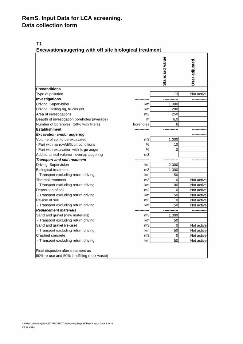
RemS. Input Data for LCA screening.Data collection form
T1
Excavation/augering with off site biological treatment
Sta
nd
ard
valu
e
Us
er
ad
jus
ted
Preconditions
Type of pollution Oil Not active
Investigations ------------ ------------ ------------
Driving. Supervision km 1.000
Driving. Drilling rig, trucks ect. km 200
Area of investigations m2 250
Deapth of investigation boreholes (average) m 6,0
Number of boreholes. (50% with filters) boreholes 6
Establishment ------------ ------------ ------------
Excavation and/or augering ------------
Volume of soil to be excavated m3 1.000
- Part with narrow/difficult conditions % 10
- Part with excavation with large auger % 0
Additional soil volume - overlap augering m3
Transport and soil treatment ------------ ------------ ------------
Driving. Supervision km 2.000
Biological treatment m3 1.000
- Transport excluding return driving km 50
Thermal treatment m3 0 Not active
- Transport excluding return driving km 100 Not active
Deposition of soil m3 0 Not active
- Transport excluding return driving km 50 Not active
Re-use of soil m3 0 Not active
- Transport excluding return driving km 50 Not active
Replacement materials ------------ ------------ ------------
Sand and gravel (new materials) m3 1.000
- Transport excluding return driving km 50
Sand and gravel (re-use) m3 0 Not active
- Transport excluding return driving km 50 Not active
Crushed concrete m3 0 Not active
- Transport excluding return driving km 50 Not active
Final disposion after treatment as
50% re-use and 50% landfilling (bulk waste)
\\allkfs01\data\sag\203\867\PROJECT\Vejledning\Engelsk\RemS Input Data 2_0.xls
30-03-2011
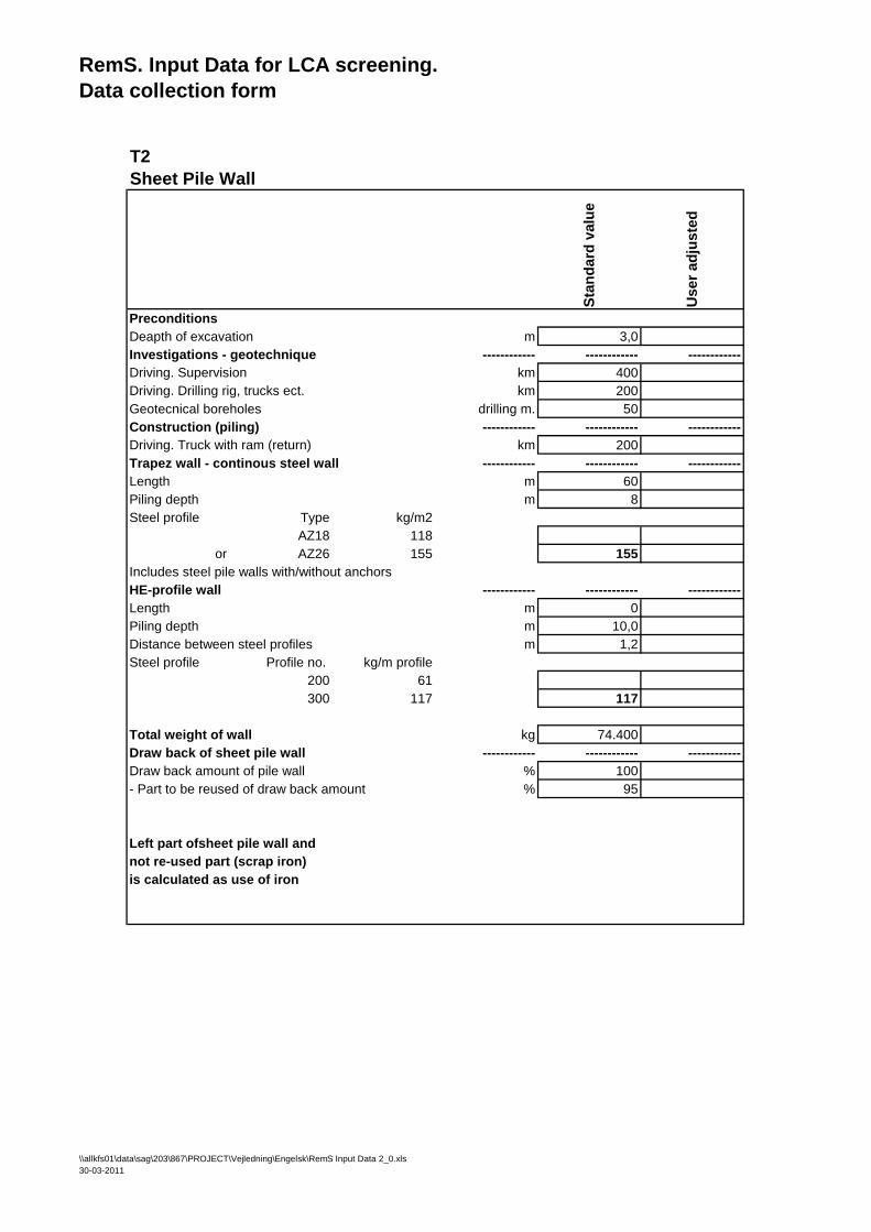
RemS. Input Data for LCA screening.Data collection form
T2
Sheet Pile Wall
Sta
nd
ard
valu
e
Us
er
ad
jus
ted
Preconditions
Deapth of excavation m 3,0
Investigations - geotechnique ------------ ------------ ------------
Driving. Supervision km 400
Driving. Drilling rig, trucks ect. km 200
Geotecnical boreholes drilling m. 50
Construction (piling) ------------ ------------ ------------
Driving. Truck with ram (return) km 200
Trapez wall - continous steel wall ------------ ------------ ------------
Length m 60
Piling depth m 8
Steel profile Type kg/m2
AZ18 118
or AZ26 155 155
Includes steel pile walls with/without anchors
HE-profile wall ------------ ------------ ------------
Length m 0
Piling depth m 10,0
Distance between steel profiles m 1,2
Steel profile Profile no. kg/m profile
200 61
300 117 117
Total weight of wall kg 74.400
Draw back of sheet pile wall ------------ ------------ ------------
Draw back amount of pile wall % 100
- Part to be reused of draw back amount % 95
Left part ofsheet pile wall and
not re-used part (scrap iron)
is calculated as use of iron
\\allkfs01\data\sag\203\867\PROJECT\Vejledning\Engelsk\RemS Input Data 2_0.xls
30-03-2011
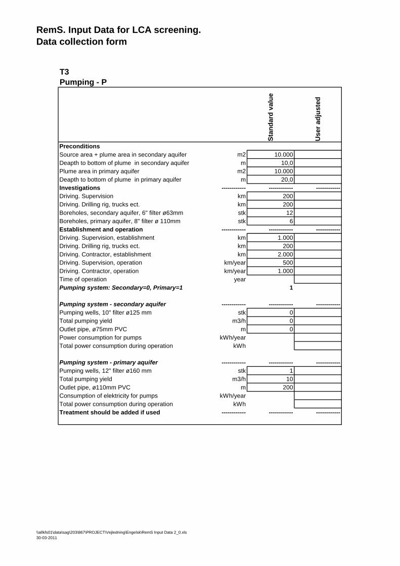
RemS. Input Data for LCA screening.Data collection form
T3
Pumping - P
Sta
nd
ard
valu
e
Us
er
ad
jus
ted
Preconditions
Source area + plume area in secondary aquifer m2 10.000
Deapth to bottom of plume in secondary aquifer m 10,0
Plume area in primary aquifer m2 10.000
Deapth to bottom of plume in primary aquifer m 20,0
Investigations ------------ ------------ ------------
Driving. Supervision km 200
Driving. Drilling rig, trucks ect. km 200
Boreholes, secondary aquifer, 6" filter ø63mm stk 12
Boreholes, primary aquifer, 8" filter ø 110mm stk 6
Establishment and operation ------------ ------------ ------------
Driving. Supervision, establishment km 1.000
Driving. Drilling rig, trucks ect. km 200
Driving. Contractor, establishment km 2.000
Driving. Supervision, operation km/year 500
Driving. Contractor, operation km/year 1.000
Time of operation year
Pumping system: Secondary=0, Primary=1 1
Pumping system - secondary aquifer ------------ ------------ ------------
Pumping wells, 10" filter ø125 mm stk 0
Total pumping yield m3/h 0
Outlet pipe, ø75mm PVC m 0
Power consumption for pumps kWh/year
Total power consumption during operation kWh
Pumping system - primary aquifer ------------ ------------ ------------
Pumping wells, 12" filter ø160 mm stk 1
Total pumping yield m3/h 10
Outlet pipe, ø110mm PVC m 200
Consumption of elektricity for pumps kWh/year
Total power consumption during operation kWh
Treatment should be added if used ------------ ------------ ------------
\\allkfs01\data\sag\203\867\PROJECT\Vejledning\Engelsk\RemS Input Data 2_0.xls
30-03-2011
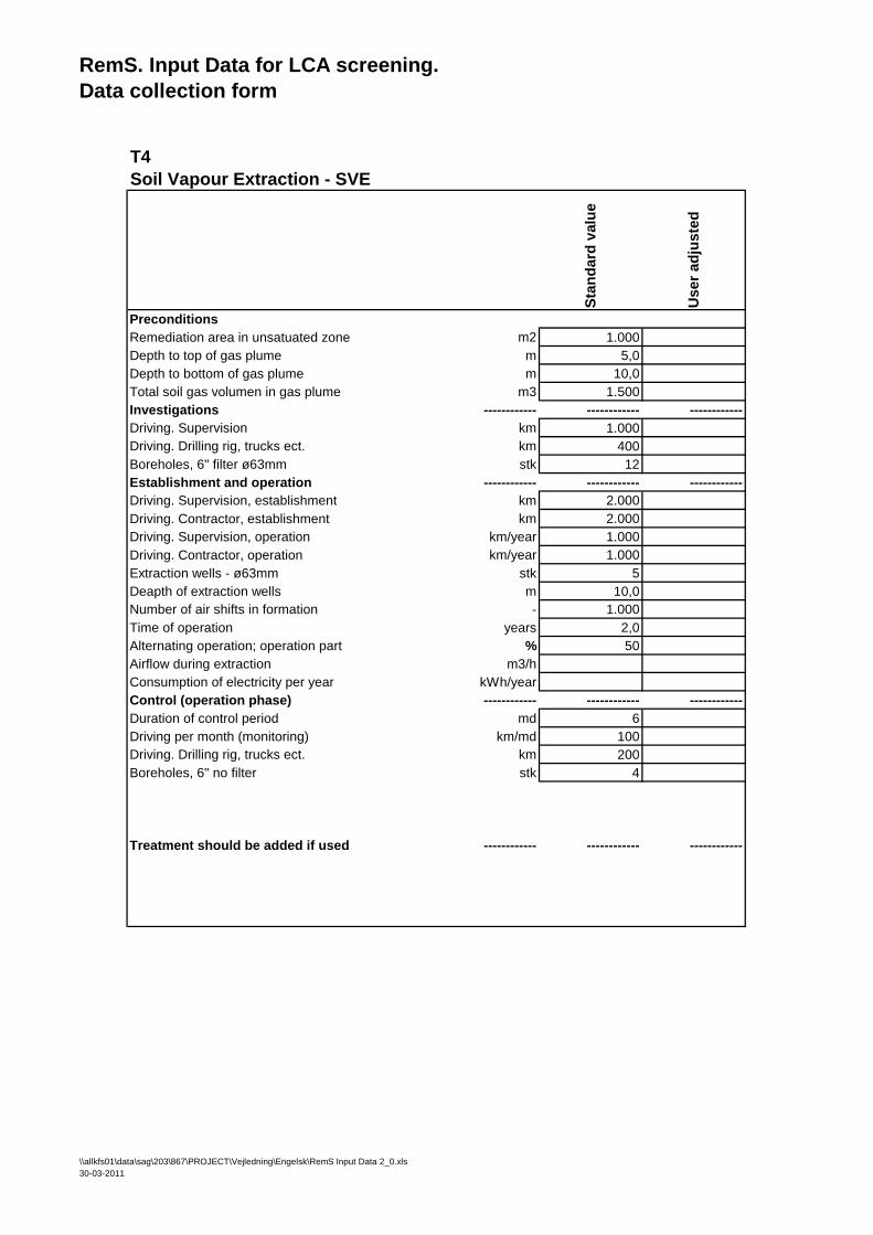
RemS. Input Data for LCA screening.Data collection form
T4
Soil Vapour Extraction - SVE
Sta
nd
ard
valu
e
Us
er
ad
jus
ted
Preconditions
Remediation area in unsatuated zone m2 1.000
Depth to top of gas plume m 5,0
Depth to bottom of gas plume m 10,0
Total soil gas volumen in gas plume m3 1.500
Investigations ------------ ------------ ------------
Driving. Supervision km 1.000
Driving. Drilling rig, trucks ect. km 400
Boreholes, 6" filter ø63mm stk 12
Establishment and operation ------------ ------------ ------------
Driving. Supervision, establishment km 2.000
Driving. Contractor, establishment km 2.000
Driving. Supervision, operation km/year 1.000
Driving. Contractor, operation km/year 1.000
Extraction wells - ø63mm stk 5
Deapth of extraction wells m 10,0
Number of air shifts in formation - 1.000
Time of operation years 2,0
Alternating operation; operation part % 50
Airflow during extraction m3/h
Consumption of electricity per year kWh/year
Control (operation phase) ------------ ------------ ------------
Duration of control period md 6
Driving per month (monitoring) km/md 100
Driving. Drilling rig, trucks ect. km 200
Boreholes, 6" no filter stk 4
Treatment should be added if used ------------ ------------ ------------
\\allkfs01\data\sag\203\867\PROJECT\Vejledning\Engelsk\RemS Input Data 2_0.xls
30-03-2011
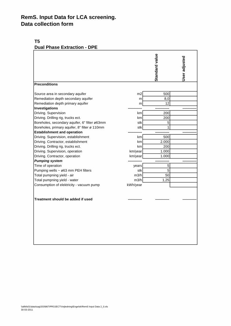
RemS. Input Data for LCA screening.Data collection form
T5
Dual Phase Extraction - DPE
Sta
nd
ard
valu
e
Us
er
ad
jus
ted
Preconditions
Source area in secondary aquifer m2 500
Remediation depth secondary aquifer m 8,0
Remediation depth primary aquifer m 12
Investigations ------------ ------------ ------------
Driving. Supervision km 200
Driving. Drilling rig, trucks ect. km 200
Boreholes, secondary aquifer, 6" filter ø63mm stk 5
Boreholes, primary aquifer, 8" filter ø 110mm stk 1
Establishment and operation ------------ ------------ ------------
Driving. Supervision, establishment km 500
Driving. Contractor, establishment km 2.000
Driving. Drilling rig, trucks ect. km 200
Driving. Supervision, operation km/year 1.000
Driving. Contractor, operation km/year 1.000
Pumping system ------------ ------------ ------------
Time of operation years 5
Pumping wells ~ ø63 mm PEH filters stk 5
Total pumpning yield - air m3/h 50
Total pumpning yield - water m3/h 1,25
Consumption of elektricity - vacuum pump kWh/year
Treatment should be added if used ------------ ------------ ------------
\\allkfs01\data\sag\203\867\PROJECT\Vejledning\Engelsk\RemS Input Data 2_0.xls
30-03-2011
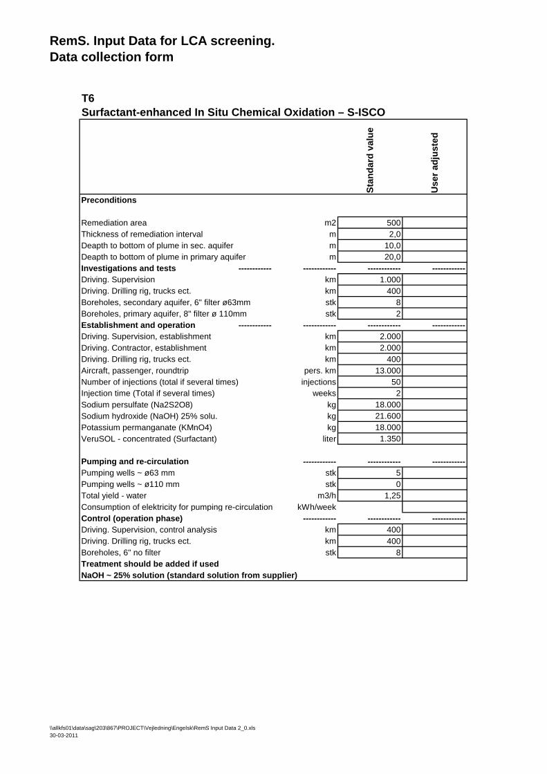
RemS. Input Data for LCA screening.Data collection form
T6
Surfactant-enhanced In Situ Chemical Oxidation – S-ISCO
Sta
nd
ard
valu
e
Us
er
ad
jus
ted
Preconditions
Remediation area m2 500
Thickness of remediation interval m 2,0
Deapth to bottom of plume in sec. aquifer m 10,0
Deapth to bottom of plume in primary aquifer m 20,0
Investigations and tests ------------ ------------ ------------ ------------
Driving. Supervision km 1.000
Driving. Drilling rig, trucks ect. km 400
Boreholes, secondary aquifer, 6" filter ø63mm stk 8
Boreholes, primary aquifer, 8" filter ø 110mm stk 2
Establishment and operation ------------ ------------ ------------ ------------
Driving. Supervision, establishment km 2.000
Driving. Contractor, establishment km 2.000
Driving. Drilling rig, trucks ect. km 400
Aircraft, passenger, roundtrip pers. km 13.000
Number of injections (total if several times) injections 50
Injection time (Total if several times) weeks 2
Sodium persulfate (Na2S2O8) kg 18.000
Sodium hydroxide (NaOH) 25% solu. kg 21.600
Potassium permanganate (KMnO4) kg 18.000
VeruSOL - concentrated (Surfactant) liter 1.350
Pumping and re-circulation ------------ ------------ ------------
Pumping wells ~ ø63 mm stk 5
Pumping wells ~ ø110 mm stk 0
Total yield - water m3/h 1,25
Consumption of elektricity for pumping re-circulation kWh/week
Control (operation phase) ------------ ------------ ------------
Driving. Supervision, control analysis km 400
Driving. Drilling rig, trucks ect. km 400
Boreholes, 6" no filter stk 8
Treatment should be added if used
NaOH ~ 25% solution (standard solution from supplier)
\\allkfs01\data\sag\203\867\PROJECT\Vejledning\Engelsk\RemS Input Data 2_0.xls
30-03-2011
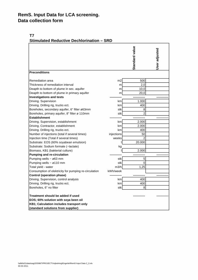
RemS. Input Data for LCA screening.Data collection form
T7
Stimulated Reductive Dechlorination – SRD
Sta
nd
ard
valu
e
Us
er
ad
jus
ted
Preconditions
Remediation area m2 500
Thickness of remediation interval m 2,0
Deapth to bottom of plume in sec. aquifer m 10,0
Deapth to bottom of plume in primary aquifer m 20,0
Investigations and tests ------------ ------------ ------------
Driving. Supervision km 1.000
Driving. Drilling rig, trucks ect. km 400
Boreholes, secondary aquifer, 6" filter ø63mm stk 8
Boreholes, primary aquifer, 8" filter ø 110mm stk 2
Establishment ------------ ------------ ------------
Driving. Supervision, establishment km 2.000
Driving. Contractor, establishment km 2.000
Driving. Drilling rig, trucks ect. km 400
Number of injections (total if several times) injections 50
Injection time (Total if several times) weeks 2
Substrate: EOS (60% soyabean emulsion) l 20.000
Substrate: Sodium formate (~lactate) kg
Biomass, KB1 (bakterial culture) l 2.000
Pumping and re-circulation ------------ ------------ ------------
Pumping wells ~ ø63 mm stk 5
Pumping wells ~ ø110 mm stk 0
Total yield - water m3/h 1,25
Consumption of elektricity for pumping re-circulation kWh/week
Control (operation phase) ------------ ------------ ------------
Driving. Supervision, control analysis km 400
Driving. Drilling rig, trucks ect. km 400
Boreholes, 6" no filter stk 8
Treatment should be added if used ------------ ------------
EOS; 60% solution with soya been oil
KB1; Calculation includes transport only
(standard solutions from supplier)
\\allkfs01\data\sag\203\867\PROJECT\Vejledning\Engelsk\RemS Input Data 2_0.xls
30-03-2011
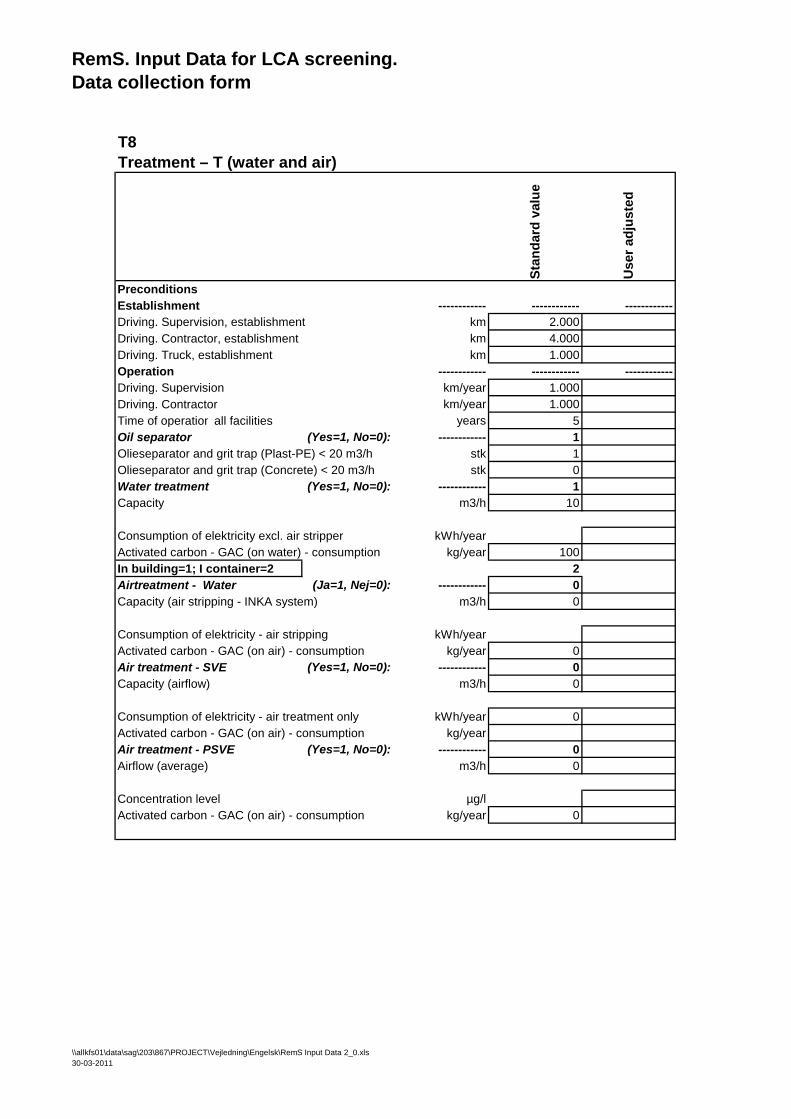
RemS. Input Data for LCA screening.Data collection form
T8
Treatment – T (water and air)
Sta
nd
ard
valu
e
Us
er
ad
jus
ted
Preconditions
Establishment ------------ ------------ ------------
Driving. Supervision, establishment km 2.000
Driving. Contractor, establishment km 4.000
Driving. Truck, establishment km 1.000
Operation ------------ ------------ ------------
Driving. Supervision km/year 1.000
Driving. Contractor km/year 1.000
Time of operation all facilities years 5
Oil separator (Yes=1, No=0): ------------ 1
Olieseparator and grit trap (Plast-PE) < 20 m3/h stk 1
Olieseparator and grit trap (Concrete) < 20 m3/h stk 0
Water treatment (Yes=1, No=0): ------------ 1
Capacity m3/h 10
Consumption of elektricity excl. air stripper kWh/year
Activated carbon - GAC (on water) - consumption kg/year 100
In building=1; I container=2 2
Airtreatment - Water (Ja=1, Nej=0): ------------ 0
Capacity (air stripping - INKA system) m3/h 0
Consumption of elektricity - air stripping kWh/year
Activated carbon - GAC (on air) - consumption kg/year 0
Air treatment - SVE (Yes=1, No=0): ------------ 0
Capacity (airflow) m3/h 0
Consumption of elektricity - air treatment only kWh/year 0
Activated carbon - GAC (on air) - consumption kg/year
Air treatment - PSVE (Yes=1, No=0): ------------ 0
Airflow (average) m3/h 0
Concentration level µg/l
Activated carbon - GAC (on air) - consumption kg/year 0
\\allkfs01\data\sag\203\867\PROJECT\Vejledning\Engelsk\RemS Input Data 2_0.xls
30-03-2011
RemS. Input Data for LCA screening.Data collection form
T9
Soil mixing with Zero Valent Iron – ZVI
Sta
nd
ard
valu
e
Us
er
ad
jus
ted
Preconditions
Remediaton area (ex. additional area - uncertainty) m2 100
Remediation depth (average) m 10,0
Investigations ------------ ------------ ------------
Driving. Supervision km 500
Driving. Drilling rig, trucks ect. km 400
Boreholes, 6" filter ø63mm stk 25
Establishment ------------ ------------ ------------
Driving. Supervision km 2.000
Driving. Drilling rig, trucks ect. km 2.000
Driving. Heavy transport km 200
Working days, soilmixing days 10
Reaktive substance, ZVI (micro scale) kg 57.000
Stabilizing agent, bentonit Taasinge, DK kg 19.000
Stabilizing agent, bentonit Mikolit, DE/BE kg
Control (operation phase) ------------ ------------ ------------
Driving. Supervision, control analysis km 500
Driving. Drilling rig, trucks ect. km 200
Boreholes, 6" no filter stk 25
\\allkfs01\data\sag\203\867\PROJECT\Vejledning\Engelsk\RemS Input Data 2_0.xls
30-03-2011
RemS. Input Data for LCA screening.Data collection form
T10
Natural Attenuation - NA
Sta
nd
ard
valu
e
Us
er
ad
jus
ted
Preconditions
Area of pollution m2 500
Bottom level of monitoring, secondary aquifer m 10
Thickness of remediation interval m 4,0
Bottom level of monitoring, primary aquifer m 20
Thickness of remediation interval m 4,0
Investigations (establishment) ------------ ------------ ------------
Driving. Supervision km 1.000
Driving. Drilling rig, trucks ect. km 500
Boreholes, secondary aquifer, 6" filter ø63mm stk 10
Boreholes, primary aquifer, 8" filter ø 110mm stk 2
Monitoring (operation phase) ------------ ------------ ------------
Time of operation years 5
Driving. Supervision, control analysis km/year 1.000
Control (operation phase) ------------ ------------ ------------
Driving. Supervision, control analysis km 400
Driving. Drilling rig, trucks ect. km 400
Boreholes, 6" no filter stk 8
\\allkfs01\data\sag\203\867\PROJECT\Vejledning\Engelsk\RemS Input Data 2_0.xls
30-03-2011
RemS. Input Data for LCA screening.Data collection form
T11Passive Soil Vapour Extraction – PSVE
Sta
nd
ard
valu
e
Us
er
ad
jus
ted
Preconditions
Remediation area in unsatuated zone m2 1.000
Depth to top of gas plume m 5,0
Depth to bottom of gas plume m 10,0
Total soil gas volumen in gas plume m3 1.500
Investigations ------------ ------------ ------------
Driving. Supervision km 1.000
Driving. Drilling rig, trucks ect. km 400
Boreholes, 6" filter ø63mm stk 12
Establishment and operation ------------ ------------ ------------
Driving. Supervision, establishment km 1.000
Driving. Contractor, establishment km 1.000
Driving. Supervision, operation km/year 200
Driving. Contractor, operation km/year 500
Extraction wells - ø63mm stk 10
Extraction capacity per well m3/h 2,0
Depth of extraction wells m 10,0
Number of air shifts in formation - 1.000
Time of operation years 10
Control (operation phase) ------------ ------------ ------------
Driving. Drilling rig, trucks ect. km 200
Boreholes, 6" no filter stk 4
\\allkfs01\data\sag\203\867\PROJECT\Vejledning\Engelsk\RemS Input Data 2_0.xls
30-03-2011
RemS. Input Data for LCA screening.Data collection form
T12In Situ Thermal Desorption - ISTD (conductive heating)
Sta
nd
ard
valu
e
Us
er
ad
jus
ted
Preconditions
Remediaton area (ex. additional area - uncertainty) m2 500
Remediation depth (average) m 7,0
Investigations ------------ ------------ ------------
Driving. Supervision km 500
Driving. Drilling rig, trucks ect. km 400
Boreholes, 6" filter ø63mm stk 25
Establishment ------------ ------------ ------------
Driving. Supervision km 2.000
Driving. Drilling rig, trucks ect. km 400
Depth to top level to be heated (average) m 0,0
Depth to bottom level to be heated (average) m 8,5
Heating wells, Direct Push, ø89 Heatercan stk 44
Temperature monitoring probes, Direct Push, 1" filter stk 14
Vacuum venting wells, 8" stk 14
Pressure monitoring probes, 1 m , 1 " filter stk 6
Vapor drain - sand/gravel layer, 0,1 m thick m3 50
Vaporcap, 0,2 m foam concrete (~400 kg/m3) m3 100
Operation ------------ ------------ ------------
Consumption of elektricity for soil heating MWh 1.275
Consumption of elektricity for other purposes ------------ ------------ ------------
Time of operation weeks 21
Operating power for other electric units kW 80
Consumption of elektricity for other electric units MWh 282
Retention capacity on GAC - air treatment % 15
Consumption of GAC - air treatment kg
Consumption of GAC - water treatment % 5
Driving per week. Supervision, service km/week 500
Driving per week. Truck, service km/week 100
Control (operation phase) ------------ ------------ ------------
Driving. Supervision, control analysis km 500
Driving. Drilling rig, trucks ect. km 200
Boreholes, 6" no filter stk 25
\\allkfs01\data\sag\203\867\PROJECT\Vejledning\Engelsk\RemS Input Data 2_0.xls
30-03-2011
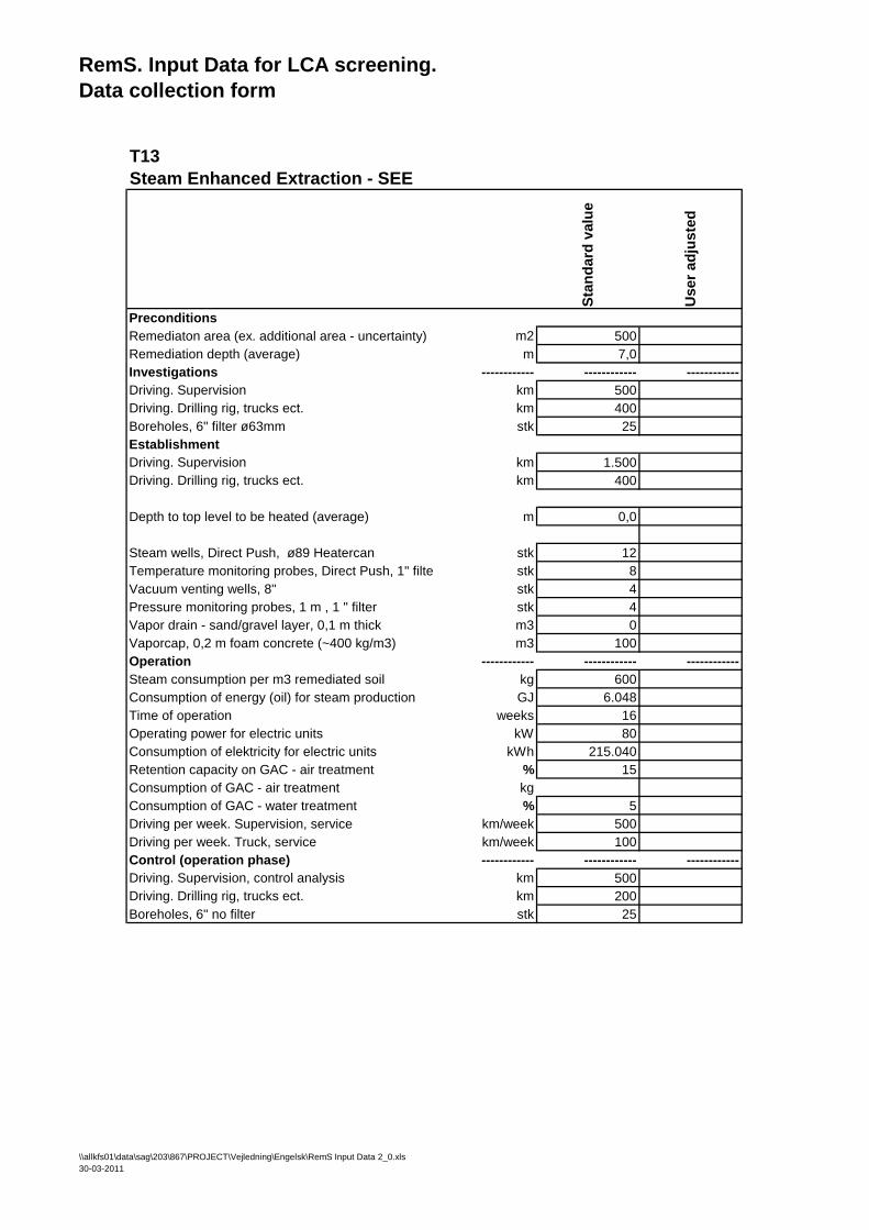
RemS. Input Data for LCA screening.Data collection form
T13
Steam Enhanced Extraction - SEE
Sta
nd
ard
valu
e
Us
er
ad
jus
ted
Preconditions
Remediaton area (ex. additional area - uncertainty) m2 500
Remediation depth (average) m 7,0
Investigations ------------ ------------ ------------
Driving. Supervision km 500
Driving. Drilling rig, trucks ect. km 400
Boreholes, 6" filter ø63mm stk 25
Establishment
Driving. Supervision km 1.500
Driving. Drilling rig, trucks ect. km 400
Depth to top level to be heated (average) m 0,0
Steam wells, Direct Push, ø89 Heatercan stk 12
Temperature monitoring probes, Direct Push, 1" filter stk 8
Vacuum venting wells, 8" stk 4
Pressure monitoring probes, 1 m , 1 " filter stk 4
Vapor drain - sand/gravel layer, 0,1 m thick m3 0
Vaporcap, 0,2 m foam concrete (~400 kg/m3) m3 100
Operation ------------ ------------ ------------
Steam consumption per m3 remediated soil kg 600
Consumption of energy (oil) for steam production GJ 6.048
Time of operation weeks 16
Operating power for electric units kW 80
Consumption of elektricity for electric units kWh 215.040
Retention capacity on GAC - air treatment % 15
Consumption of GAC - air treatment kg
Consumption of GAC - water treatment % 5
Driving per week. Supervision, service km/week 500
Driving per week. Truck, service km/week 100
Control (operation phase) ------------ ------------ ------------
Driving. Supervision, control analysis km 500
Driving. Drilling rig, trucks ect. km 200
Boreholes, 6" no filter stk 25
\\allkfs01\data\sag\203\867\PROJECT\Vejledning\Engelsk\RemS Input Data 2_0.xls
30-03-2011
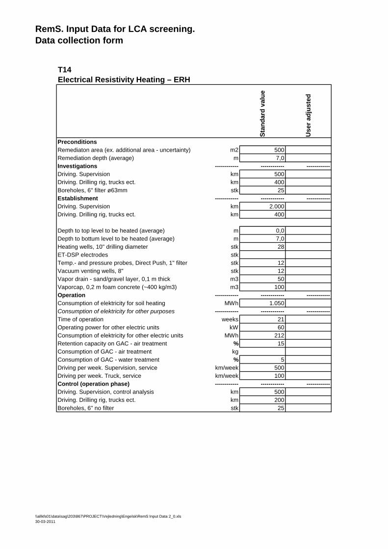
RemS. Input Data for LCA screening.Data collection form
T14
Electrical Resistivity Heating – ERH
Sta
nd
ard
valu
e
Us
er
ad
jus
ted
Preconditions
Remediaton area (ex. additional area - uncertainty) m2 500
Remediation depth (average) m 7,0
Investigations ------------ ------------ ------------
Driving. Supervision km 500
Driving. Drilling rig, trucks ect. km 400
Boreholes, 6" filter ø63mm stk 25
Establishment ------------ ------------ ------------
Driving. Supervision km 2.000
Driving. Drilling rig, trucks ect. km 400
Depth to top level to be heated (average) m 0,0
Depth to bottum level to be heated (average) m 7,0
Heating wells, 10" drilling diameter stk 28
ET-DSP electrodes stk
Temp.- and pressure probes, Direct Push, 1" filter stk 12
Vacuum venting wells, 8" stk 12
Vapor drain - sand/gravel layer, 0,1 m thick m3 50
Vaporcap, 0,2 m foam concrete (~400 kg/m3) m3 100
Operation ------------ ------------ ------------
Consumption of elektricity for soil heating MWh 1.050
Consumption of elektricity for other purposes ------------ ------------ ------------
Time of operation weeks 21
Operating power for other electric units kW 60
Consumption of elektricity for other electric units MWh 212
Retention capacity on GAC - air treatment % 15
Consumption of GAC - air treatment kg
Consumption of GAC - water treatment % 5
Driving per week. Supervision, service km/week 500
Driving per week. Truck, service km/week 100
Control (operation phase) ------------ ------------ ------------
Driving. Supervision, control analysis km 500
Driving. Drilling rig, trucks ect. km 200
Boreholes, 6" no filter stk 25
\\allkfs01\data\sag\203\867\PROJECT\Vejledning\Engelsk\RemS Input Data 2_0.xls
30-03-2011
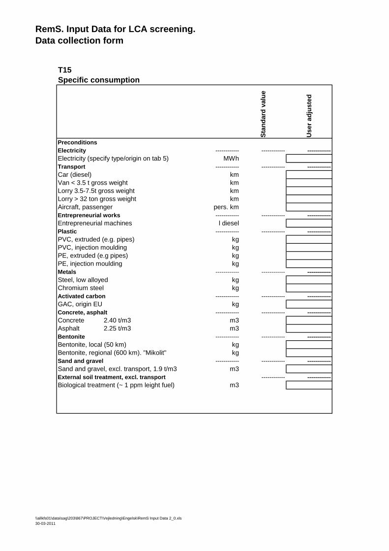
RemS. Input Data for LCA screening.Data collection form
T15
Specific consumption
Sta
nd
ard
valu
e
Us
er
ad
jus
ted
Preconditions
Electricity ------------ ------------ ------------
Electricity (specify type/origin on tab 5) MWhTransport ------------ ------------ ------------
Car (diesel) kmVan < 3.5 t gross weight kmLorry 3.5-7.5t gross weight kmLorry > 32 ton gross weight kmAircraft, passenger pers. kmEntrepreneurial works ------------ ------------ ------------
Entrepreneurial machines l dieselPlastic ------------ ------------ ------------
PVC, extruded (e.g. pipes) kgPVC, injection moulding kgPE, extruded (e.g pipes) kgPE, injection moulding kgMetals ------------ ------------ ------------
Steel, low alloyed kgChromium steel kgActivated carbon ------------ ------------ ------------
GAC, origin EU kgConcrete, asphalt ------------ ------------ ------------
Concrete 2.40 t/m3 m3Asphalt 2.25 t/m3 m3Bentonite ------------ ------------ ------------
Bentonite, local (50 km) kgBentonite, regional (600 km). "Mikolit" kgSand and gravel ------------ ------------ ------------
Sand and gravel, excl. transport, 1.9 t/m3 m3External soil treatment, excl. transport ------------ ------------
Biological treatment (~ 1 ppm leight fuel) m3
\\allkfs01\data\sag\203\867\PROJECT\Vejledning\Engelsk\RemS Input Data 2_0.xls
30-03-2011