removing shadows from images - ok.sc.e.titech.ac.jp · project report removing shadows from images...
TRANSCRIPT

ECSE-529AImage Processing and Communication
Project Report
Removing Shadows from Images
by
Samuel Audet
December 2, 2005

ECSE-529AImage Processing and Communication
Instructor: M. D. Levine
Project Report
Removing Shadows from Images
by
Samuel [email protected]
ID: 260184380
December 2, 2005
Electrical and Computer Engineering Department3480 University Street Room 410
Montreal, QuebecCanada H3A 2A7

ABSTRACT
Removing Shadows from Images
Samuel Audet
For this project, the shadow removal method used by Finlayson et al. in [1] was imple-
mented. This report contains an overview of the mathematical background and a detailed
discussion on the experiments performed with the implementation.
This method consists of two independent steps. First, an illumination invariant image
is derived from a color image for which an appropriate color calibration is known. Second,
shadow edges are detected by finding edges in the intensity image that are not in the illu-
mination invariant image. Gradient information is then erased at those shadow edges, and
a new shadowless color image is formed by solving a Poisson’s equation.
ii

ACKNOWLEDGMENTS
I would like to thank Professor Martin D. Levine for teaching the Image Processing course
from which I learned a lot of interesting material. I also gratefully acknowledge help received
from Stephane Pelletier and Professor Paul Tupper with regards to understanding some of
the mathematical background. Thanks as well to Jonathan Miller for proofreading this
report.
iii

Contents
List of Figures v
1 Introduction 1
2 Literature Review 2
3 Shadow Removal Theory 4
4 Experimentation and Discussion 8
4.1 Artificial Test Images . . . . . . . . . . . . . . . . . . . . . . . . . . . . . . . 8
4.2 Real World Images . . . . . . . . . . . . . . . . . . . . . . . . . . . . . . . . 11
5 Conclusion 17
References 20
iv

List of Figures
4.1 First test image processed with σ = 3, t1 = 5, t2 = 5, r1 = 1, r2 = 3 . . . . . 8
4.2 First test image processed with σ = 3, t1 = 5, t2 = 5, r1 = 1, r2 = 24 . . . . 9
4.3 Second test image processed with σ = 3, t1 = 5, t2 = 5, r1 = 1, r2 = 3 . . . . 10
4.4 Second test image processed with σ = 15, t1 = 5, t2 = 5, r1 = 1, r2 = 3 . . . 10
4.5 merry0101.tif processed with σ = 5, t1 = 5, t2 = 10, r1 = 2, r2 = 15 . . . . . 12
4.6 merry0107.tif processed with σ = 3, t1 = 15, t2 = 15, r1 = 1, r2 = 5 . . . . . 13
4.7 merry florida0005.tif processed with σ = 3, t1 = 15, t2 = 15, r1 = 1, r2 = 5 . 13
4.8 merry italy0146.tif processed with σ = 5, t1 = 7, t2 = 10, r1 = 1, r2 = 5 . . . 14
4.9 merry italy0188.tif processed with σ = 3, t1 = 15, t2 = 10, r1 = 1, r2 = 5 . . 14
4.10 merry mexico0140.tif processed with σ = 7, t1 = 3, t2 = 7, r1 = 1, r2 = 5 . . 15
4.11 merry italy0052.tif processed with σ = 3, t1 = 15, t2 = 15, r1 = 1, r2 = 5 . . 15
4.12 merry winter0033.tif processed with σ = 5, t1 = 5, t2 = 10, r1 = 1, r2 = 5 . . 16
v

Chapter 1
IntroductionShadows have always plagued computer vision applications where tracking, segmentation,
detection and recognition algorithms confuse the boundaries of shadows with those of differ-
ent surfaces or objects. It is therefore of great interest to discover ways of properly detecting
shadows and removing them while leaving other details of the original image untouched. The
ideal shadowless image would be an image where, although shading occurs due to the texture
of the material, large patches of shadows are removed, effectively taking out the direction of
the illumination, and leaving only the reflectance and the locally shaded texture. It is this
goal that the shadow removal method of Finlayson et al. [1] attempts to achieve.
For this project, the shadow removal method of Finlayson et al. was implemented, and
experiments were conducted. However, before discussing the results of those experiments,
first a literature review providing an overview of other methods used to achieve similar
goals are briefly explained and critically evaluated with regards to their advantages and
disadvantages. Then, the theoretical background of the method of interest in this report
is briefly explained. It is composed of two independent steps. The first step consists in
deriving an illumination invariant image from a color image. This step requires the knowledge
of a color calibration appropriate to this method. In the second step, the shadow edges
are detected and used to produce a new gradient image which is integrated by solving
the Poisson’s equation to recover the new shadowless color image. Finally, experimental
results showing how close the method is at achieving its goal are discussed while detailing its
capabilities and limitations for both test images and real world images. Although in some
cases the method offers acceptable results, it is far too sensitive to busy images, images where
the Planckian lighting assumption does not hold, or camera sensors whose responses are not
sufficiently narrow. The method also fails to remove shadows with very smooth edges.
1

Chapter 2
Literature ReviewA lot of research on shadow detection has been performed, but not as much was done on
shadow removal. The interest of shadow removal is not limited to the detection of the
shadow. It is also sometimes important to find ways to remove the effect of the shadow
while still keeping the underlying texture of the surfaces. For example, in applications where
both tracking and recognition of objects are important, one would might wish to keep the
shading of textured surfaces intact, while discounting the effect of sharp shadows casted
upon those surfaces.
Work by Weiss in [2] demonstrates how to recover intrinsic illumination and reflectance
images under the assumption that the histogram of the illumination and intensity derivatives
are sparse, meaning most of the values are 0. A sequence of images with illumination changes,
where shadow edges move, but with no reflectance changes, where all the surfaces and objects
do not move, go through derivation filters. For each pixel, only the median of this sequence
is kept, amounting to the maximum-likelihood estimation of the invariant reflectance. While
this method computes very natural looking, shadowless images, it does not work on single
images, or on a sequence where illumination does not change or where the reflectance does.
Levine et al. in [3] show a method making various assumptions about the behavior
of shadows at their boundaries, and segment images into shadow and non-shadow regions
with the help of a manually trained support vector machine. After some post-processing,
continuous and closed boundaries are found, and pixel color within the shadow regions are
replaced with the average color found at the boundaries. Unfortunately, this method removes
all high frequency details from the shadow regions and amounts to a very strong smoothing
of the reflectance.
The goal of work done by Sasagawa et al. in [4] is to remove shadows from satellite images
where geometric information of the scene and of the light source, the sun, are known. A
model of casted shadows can thus be precomputed with this knowledge, but it is impractical
for general purposes where no geometric information is known.
Tappen et al. in [5] build derivative images of the ”shading” (gray-scale illumination)
and of the reflectance. They use a color classifier based on the invariance properties of
normalized RGB and a manually trained grayscale classifier based on a local analysis of
2

edges with the help of the AdaBoost algorithm to find optimal filters and thresholds. The
resulting derivatives are then integrated in the same way as in [2], giving quite good results.
This method, however, tends to remove a lot of texture information from the reflectance
image.
The ShadowFlash algorithm [6] effectively removes shadows from scenes in an active
manner by illuminating an object or a scene from several different angles. Although it
produces very good results, it is an active technique and is not applicable to images in
general.
3

Chapter 3
Shadow Removal TheoryTwo independent steps are involved in the shadow removal method of Finlayson et al. [1].
The first step consists in performing operations to get an illumination invariant image, which
is a grayscale representation proportional to the color reflectance of the surfaces. To work
properly, this step requires some color calibration as well as other conditions described below.
The second step consists in finding shadow edges and removing them from the color image.
Shadow edges are defined as edges that are part of the intensity image, but not of the
illumination invariant image. With these shadow edges, it is possible to stamp these edges
off from the gradient of each color channel, and to recover a shadowless color image by solving
a linear system approximating the Poisson’s equation to integrate the now shadowless image
from the modified gradient information.
To produce the illumination invariant image, there are a few assumptions made. First, a
color calibrated camera whose sensor responses are directly proportional to the luminance is
used (but it will be shown that a more loosely defined calibration is sufficient); second, the
scene is illuminated with Planckian lighting; third, the sensor responses of the camera are
fairly narrow. To understand how this procedure works, recall that the intensity measured
by a sensor is given by
ρk =
∫E(λ)S(λ)Qk(λ)dλ where k = R,G, orB, (3.1)
and E(λ) is the spectral power distribution of the illumination, S(λ) is the surface re-
flectance distribution, and Qk(λ) is the sensor sensitivity distribution. If the sensor response
is narrow enough, it can be approximated by a Dirac delta function: Qk(λ) ≈ qkδ(λ − λk),
where qk = Q(λk) is the maximum response of the sensor at λk. Therefore,
ρk ≈ E(λk)S(λk)qk. (3.2)
Moreover, assume the lighting can be approximated by Planck’s law:
E(λ) =I2hc2
λ5
1
ehc
λkT − 1(3.3)
where T is the temperature of the black body, h is Planck’s constant, c is the speed of
light, k is Boltzmann’s constant, and I a factor representing the incident intensity of the
4

light. Through manipulation of equations (3.2) and (3.3) with three intensities from the
three color channels, one can demonstrate [1] that
gs = c1 lnρR
ρG
− c2 lnρB
ρG
where c1 =1
λB
− 1
λG
and c2 =1
λR
− 1
λG
(3.4)
is illumination invariant and solely depends on the reflectance of the surface. In this
representation, big numbers in absolute value tend to represent colorful surfaces, and colorless
surfaces (white, gray and black) tend to have lower values.
The second step consists of stamping out the border of the shadows, which are called
shadow edges. The SUSAN edge detector [7] is used to find those shadow edges. The
edge detector first blurs the image using a Gaussian kernel of given parameter σ, and then
runs the SUSAN thresholding operation. Only the strongest edges are kept, and no other
operations from the SUSAN algorithm are performed. Any edges found in the intensity
image I = (R + G + B)/3 not found in the illumination invariant image are assumed to be
shadow edges. Small noisy edges are eliminated with a morphological opening operation.
Due to the penumbra, shadow edges are not always sharp [3], so a thicker edge representation
is required. To accomplish this, a morphological dilation operation is used to thicken the
shadow edges.
Next, taking the gradient of the image in the log domain and setting pixels corresponding
to shadow edges to 0 effectively stamps out those edges. The reason this works is because,
according to equation (3.2), if one makes the assumption that S(λ), the reflectance, does
not change (which means the shadow is casted within the surface boundaries), then what is
left after taking the finite difference of two such log-domain pixels (done as part of the gra-
dient computation) is the difference in illumination E(λ). This is akin to lightness recovery
methods. The shadow edges thus drive the following algorithm :
∇sl′(x, y) =
0 if se(x, y) > 0
∇ρ′(x, y) otherwise(3.5)
where sl′(x, y) is the shadowless image in the log domain, se(x, y) are the shadow edges,
and ∇ρ′(x, y) = ∇ ln ρ(x, y). This gradient is approximated by convolution with masks[1 0 −1
]for ∇x and
[−1 0 1
]T
for ∇y. This procedure therefore removes the dif-
ference in illumination at shadow edges, if the invariant reflectance assumption holds. This
is done for the three color channels separately.
5

After which the image is reintegrated by first computing the Laplacian of sl′(x, y) by
taking the gradient of ∇sl′(x, y), and by then solving the Poisson’s equation:
∇2sl′(x, y) = ∇ · (∇sl′(x, y)) (3.6)
using Neumann boundary conditions for which the derivative is zero. This returns
sl′(x, y), the image in the log domain of the desired shadowless image, up to an unknown
additive constant. The Neumann condition is used so shadows that extend to the edges of
the image are not pulled back to their original dark shadow values. However, due to the same
Neumann boundary condition, each value is only exact up to an unknown additive constant.
Taking the exponential esl′(x,y)+k1 = k2 sl(x, y), this translates into an unknown multiplica-
tive constant. To compensate for this loss of information, for a given channel, each pixel
value is divided by the average of the pixel values belonging to the top first percentile. This
usually produces good results. However, in this report instead of the average, the median is
used, as it proved to give better results for the input images studied.
To summarize and clarify the operations of the algorithm, here is a detailed description
of each parameter.
• c1 and c2 are the constants used to create the illumination invariant image, and are
also related to the color calibration of the camera. Once these values are established
for a given camera, they do not need to be readjusted. Moreover, the author goes on to
prove that one does not need a color calibrated camera to find working constants, and
that a working calibration step for the algorithm can consist of a sequence of images of
a scene taken under varying lighting intensities, such as an outdoor scene over a period
of a few hours [1].
• σ represents the standard deviation of the Gaussian kernel used for the smoothing
operation before shadow edge detection. Noisy images or images with a lot of high-
frequency details need a higher value. Usual values range from 1 to 7.
• t1 is the SUSAN threshold for the intensity image. In the ideal case, the resulting
intensity edges must include all shadow edges. Usual values range from 5 to 20.
• t2 is the SUSAN threshold for the illumination invariant image. In the ideal case, these
edges must contain all edges from the intensity edges, while not containing any shadow
edges. Usual values range from 5 to 20.
6

• r1 is the radius of the structuring disk element for the morphological opening operation
on the shadow edges. It should be set to the size of small noisy edges in an attempt
to erase them, while keeping real shadow edges. Usual values range from 1 to 3.
• r2 is the radius of the structuring disk element for the morphological dilation operation
on the shadow edges. It should be set to the width of real shadow edges in an attempt
to completely remove them from the gradient. Usual values range from 3 to 10.
7

Chapter 4
Experimentation and DiscussionTo demonstrate how the algorithm functions and explain its capabilities and limitations, the
output produced from a few artificial test images are first discussed. Following this, results
from real world images are shown and discussed. For display and printing purposes, processed
images are all converted back to the sRGB color space [8], which consists of applying a gamma
correction of 2.2 on images whose values are linearly related to the luminance.
4.1 Artificial Test Images
The first artificial test image as shown in figure 4.1(a) consists of an almost pure blue
background and four ellipses which represent different kinds of situations the algorithm might
face. The top first ellipse is a ”perfect shadow” in the sense that the pixel values are uniform
across the ellipse, that the shadow edge is very sharp, and that its illumination invariant
value is the same as the background. The second one is an extremely smoothed version of
the first which results in a much more spread out shadow edge. The illumination invariant
value remains unchanged since the shadow edge is now merely a linear combination of two
colors that produce the same invariant value. The third one is a slightly greener and redder
shadow, which to the naked eye is pretty similar to the first. Nonetheless, this corresponds to
(a) Input image. (b) Invariant image. (c) Shadow edges. (d) Output image.
Figure 4.1. First test image processed with σ = 3, t1 = 5, t2 = 5, r1 = 1, r2 = 3
8

the case of a bad calibration or a failure of the Planckian lighting assumption. The invariant
value for this case is thus different, as seen in figure 4.1(b) . The last ellipse consists of
a completely different color producing the same invariant value. This ellipse is a model of
a surface having different reflectance than the background, but which maps to the same
invariant value. This is an inherent limitation of the method. One can easily show from
equation (3.4) that the information from the red and blue channels is effectively summed
up, so it is always possible to inverse the values of these two channels, in accordance with
the calibration, without changing the invariant value. The algorithm is in effect red/blue
color-blind.
In the output image (figure 4.1(d)), as expected, the first ellipse has completely disap-
peared. The second one is partially attenuated, but one can see from the shadow edges in
figure 4.1(c) that the its shadow edge is not thick enough. It can be successfully removed by
increasing the parameter r2 thus increasing the width of the shadow edge, as seen in figures
4.2(c) and 4.2(d). However, increasing the morphological dilation of shadow edges to big
values will erase more gradient information found within the shadow edge. This loss of infor-
mation shows up as smearing marks in natural images as seen below. The third ellipse was
not removed because it produced no shadow edge, but moreover the green channel is severely
amplified, resulting in discoloration. This problem occurs because of the normalization per-
formed to estimate the unknown multiplicative constant after integrating the gradient with
Neumann boundary conditions. In the input image (figure 4.1(a)) the values of the green
channel are very low overall, while the highest value is found within the third ellipse. After
(a) Input image. (b) Invariant image. (c) Shadow edges. (d) Output image.
Figure 4.2. First test image processed with σ = 3, t1 = 5, t2 = 5, r1 = 1, r2 = 24
9

integration, the algorithm simply takes the highest green value and maps it to the highest
pixel value possible. Now the green in the third ellipse comes out with the brightest possible
value. Next, since this algorithm is red/blue color-blind, it comes to no surprise that the
fourth ellipse is completely gone the same way the first one was removed. However, in this
case, it is a false positive as it does not represent an actual shadow.
The second test image (figure 4.3(a)) models a very busy background with a shadow edge
running over it. As one can see in the invariant image (figure 4.3(b)), the shadow is properly
ignored and all the busy information is not discarded. Everything is fine up until the point
where shadow edges are located, figure 4.3(c). It is a disaster. The real shadow edge is not
retained and many spurious edges from the busy background crop up. The reason for this is
that, in addition to the shadow edges, the edges detected in the intensity image and the ones
detected in the invariant image are not exactly the same. The gradients of both images vary
differently, and thus the pixels of the edges do not have a one to one correspondence. The
(a) Input image. (b) Invariant image. (c) Shadow edges. (d) Output image.
Figure 4.3. Second test image processed with σ = 3, t1 = 5, t2 = 5, r1 = 1, r2 = 3
(a) Input image. (b) Invariant image. (c) Shadow edges. (d) Output image.
Figure 4.4. Second test image processed with σ = 15, t1 = 5, t2 = 5, r1 = 1, r2 = 3
10

shadow edge is found somewhere in the middle of this mess and it is erased, since it passes
on top of actual reflectance changes in the invariant image, hence the misclassification. To
compensate for such images, one has to increase the σ value associated with the smoothing
operation. With a value of 15, the shadow edge can be located with some success, as shown
in figure 4.4(c). Such intensive smoothing can, however, make shadow edges disappear in
other types of images where shadow regions are narrow.
The implementation is behaving as expected with these artificial test images so it is
believed to work properly. For further discussion on the method, in the next section, it is
tested with real world images.
4.2 Real World Images
For experiments with real world images, images from the McGill Calibrated Colour Image
Database [9] were used. The use of these already-calibrated images removed the burden of
calibration and facilitated work on the algorithmic aspects of the problem. More information
on color calibration can be found in the documentation at this site. From this documentation,
the peak sensor responses of the cameras used to take these pictures are λB = 470 nm, λG =
530 nm, and λR = 590 nm. From equation (3.4): c1 = 0.24× 10⁻¹² and c2 = −0.19× 10⁻¹²,
or after normalization: c1 = 0.78 and c2 = −0.62. Since the sensor responses are obviously
not Dirac delta functions, these values were taken as initial approximations of the optimal
values. After visually evaluating a range of values and the resulting invariant images, it was
found that the values c1 = 0.47 and c2 = −0.67 gave the best results, and so these are the
values that were used for all the images.
Starting with merry0101.tif in figure 4.5, the first prominent issue is that the invariant
image really is not that invariant, which is obvious when looking at the shadow edges in the
invariant image. In the original paper [1], the invariant images look illumination invariant,
but it does not seem to work as well with the pictures used in this report. This indicates
that the narrow sensor response approximation assumed for equation (3.2) does not hold as
well as expected. Moreover, the noise pattern in the dark area is different from the one in
the bright area. Nonetheless, even in this situation it is possible to obtain relatively good
results. The shadow edges of figure 4.5(c) and the output (figure 4.5(d)) are quite acceptable.
However, there are a few things to notice about the output image. First, the overall color is
different. This is due to the Neumann boundary conditions and the subsequent per-channel
normalization. Second, as indicated before, the portion of the gradient erased at the shadow
11

(a) Input image. (b) Invariant image. (c) Shadow edges. (d) Output image.
Figure 4.5. merry0101.tif processed with σ = 5, t1 = 5, t2 = 10, r1 = 2, r2 = 15
edges appear as smearing marks in the output image. It is assumed the reflectance does
not change when executing equation (3.5), but the reflectance does in fact change as this is
textured dirt, and the information about this texture is smoothed out, resulting in visible
smearing marks. Also, the shadow is not completely removed since the edge detector fails
to properly locate the edges in the lower right corner of the picture. Should it detect them
properly, the overall color and intensity of the image would be constant. This not being
the case, some of the original gradient information is kept, affecting the whole image, albeit
the farther away a pixel is from the error, the smaller the effect. This can be explained
by an analysis of the conditioning of the problem. The condition number of the matrix for
approximating the Laplacian and for solving the Poisson’s equation (3.6) over a square image
of resolution 512× 512 is estimated to be 15× 104, which robs the results of a maximum of
log10(15×104) = 5.2 digits of accuracy in the worst case. The solutions shown in this report
were computed using IEEE 754 double precision floating-point arithmetic, which provides
− log10(2−52) = 15.7 digits of accuracy. This demonstrates that the problem is well-posed
and not very sensitive to noise, which in this case is mainly created when manipulating the
gradient images. This well-conditioned system provides robustness to failure.
Figures 4.6 and 4.7 are very complex images that cannot be properly processed as a
whole. The busy pattern created by the leaves and the grass produces a lot of noisy edges
and interferes with the localization of shadow edges. The shadow edges on the grass or in
the leaves do not come out very cleanly or at all, as seen in figures 4.6(c) and 4.7(c). It
would be possible to use stronger smoothing to compensate. However, in this case the gist
of the shadows in these images, consisting of narrow shadows, would be smoothed out and
12

(a) Input image. (b) Invariant image. (c) Shadow edges. (d) Output image.
Figure 4.6. merry0107.tif processed with σ = 3, t1 = 15, t2 = 15, r1 = 1, r2 = 5
(a) Input image. (b) Invariant image. (c) Shadow edges. (d) Output image.
Figure 4.7. merry florida0005.tif processed with σ = 3, t1 = 15, t2 = 15, r1 = 1, r2 = 5
not detected. Therefore, the results shown in figures 4.6(d) and 4.7(d) are about the best
that can be achieved with this technique. Also notice the blue halos pouring out of some
of the leaves and flowers. The blue channel being the noisiest channel is most sensitive to
changes. The maximum value of the Laplacian of this channel is usually 3 to 4 times higher
than what is observed from the red and green channels. Abruptly modifying these values as
done by this method thus results in larger errors in this channel.
In contrast, figures 4.8 and 4.9 are images for which this procedure works well. The
images are not very busy and the shadow edges are sharp and well located by the edge
detector. It is still not perfect, and one can notice the slight discoloration. Also note that in
figure 4.9 there is a lot of shadows around the sculptures at the top. In this case, one would
actually wish to keep these shadows intact, as they offer information about the shape of the
sculptures, which is lost in the shadowless image, as seen in the output image, figure 4.9(d).
13
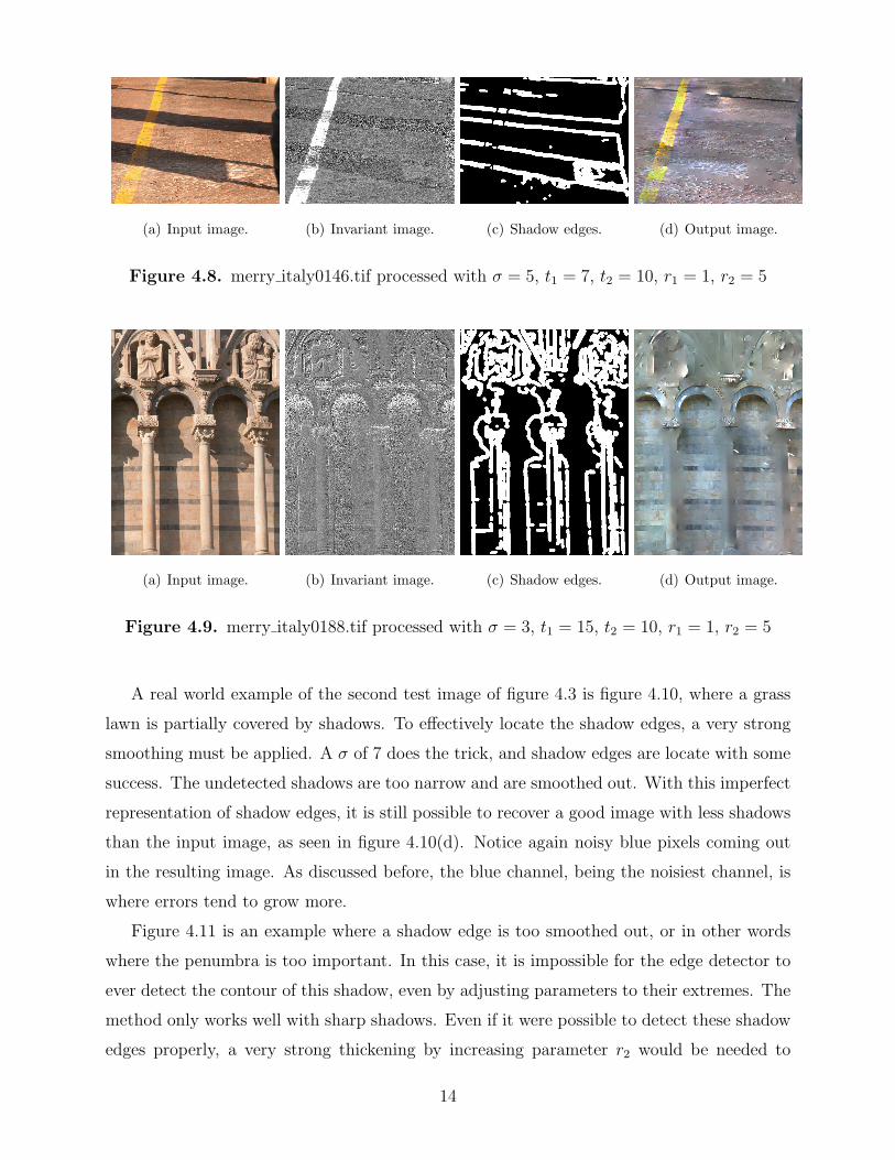
(a) Input image. (b) Invariant image. (c) Shadow edges. (d) Output image.
Figure 4.8. merry italy0146.tif processed with σ = 5, t1 = 7, t2 = 10, r1 = 1, r2 = 5
(a) Input image. (b) Invariant image. (c) Shadow edges. (d) Output image.
Figure 4.9. merry italy0188.tif processed with σ = 3, t1 = 15, t2 = 10, r1 = 1, r2 = 5
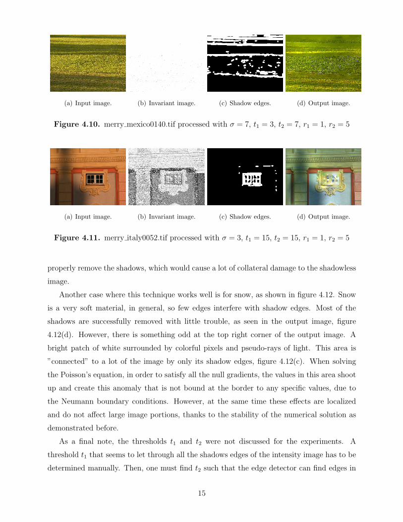
A real world example of the second test image of figure 4.3 is figure 4.10, where a grass
lawn is partially covered by shadows. To effectively locate the shadow edges, a very strong
smoothing must be applied. A σ of 7 does the trick, and shadow edges are locate with some
success. The undetected shadows are too narrow and are smoothed out. With this imperfect
representation of shadow edges, it is still possible to recover a good image with less shadows
than the input image, as seen in figure 4.10(d). Notice again noisy blue pixels coming out
in the resulting image. As discussed before, the blue channel, being the noisiest channel, is
where errors tend to grow more.
Figure 4.11 is an example where a shadow edge is too smoothed out, or in other words
where the penumbra is too important. In this case, it is impossible for the edge detector to
ever detect the contour of this shadow, even by adjusting parameters to their extremes. The
method only works well with sharp shadows. Even if it were possible to detect these shadow
edges properly, a very strong thickening by increasing parameter r2 would be needed to
14
(a) Input image. (b) Invariant image. (c) Shadow edges. (d) Output image.
Figure 4.10. merry mexico0140.tif processed with σ = 7, t1 = 3, t2 = 7, r1 = 1, r2 = 5
(a) Input image. (b) Invariant image. (c) Shadow edges. (d) Output image.
Figure 4.11. merry italy0052.tif processed with σ = 3, t1 = 15, t2 = 15, r1 = 1, r2 = 5
properly remove the shadows, which would cause a lot of collateral damage to the shadowless
image.
Another case where this technique works well is for snow, as shown in figure 4.12. Snow
is a very soft material, in general, so few edges interfere with shadow edges. Most of the
shadows are successfully removed with little trouble, as seen in the output image, figure
4.12(d). However, there is something odd at the top right corner of the output image. A
bright patch of white surrounded by colorful pixels and pseudo-rays of light. This area is
”connected” to a lot of the image by only its shadow edges, figure 4.12(c). When solving
the Poisson’s equation, in order to satisfy all the null gradients, the values in this area shoot
up and create this anomaly that is not bound at the border to any specific values, due to
the Neumann boundary conditions. However, at the same time these effects are localized
and do not affect large image portions, thanks to the stability of the numerical solution as
demonstrated before.
As a final note, the thresholds t1 and t2 were not discussed for the experiments. A
threshold t1 that seems to let through all the shadows edges of the intensity image has to be
determined manually. Then, one must find t2 such that the edge detector can find edges in
15

(a) Input image. (b) Invariant image. (c) Shadow edges. (d) Output image.
Figure 4.12. merry winter0033.tif processed with σ = 5, t1 = 5, t2 = 10, r1 = 1, r2 = 5
the invariant image which would ideally include all the edges in the intensity image except
shadow edges. However, fixing these parameters is a very subjective and error prone trial-
and-error procedure. In general, good thresholds rarely exist, and detected shadow edges
always contain a large amount of unwanted edges while real shadow edges are often broken
or not detected. Also, variation of the parameter r1 does not appear to help a lot in removing
noisy edges without damaging the shadow edges, and so was almost entirely ignored of the
discussion for this reason.
16

Chapter 5
ConclusionIn this report the shadow removal method by Finlayson et al. [1] was briefly explained,
and using an implementation of this method, experiments were conducted and a discussion
clarifying the results was given.
This method [1] consists of first deriving an illumination invariant image under the as-
sumptions of a color calibrated camera and of Planckian illumination. It was also seen that a
color calibrated camera was not necessary, and a more loosely defined calibration obtainable
from a sequence of images of a scene under varying illumination was sufficient. Second, edge
detection using the SUSAN algorithm is performed on both the intensity image and the
illumination invariant image to find shadow edges. Any edges found in the intensity image
but not in the invariant image are considered to be a shadow edges. Gradient information in
the log domain corresponding to illumination changes is removed from the image by setting
to 0 the magnitude of the gradient at pixels belonging to a thickened version of these shadow
edges. The new shadowless image is then integrated from this modified gradient.
Apart from the requirements of color calibration and Planckian lighting, there are a few
other problems with this shadow removal method. First, the sensor response of the camera
must be sufficiently narrow to provide a good illumination invariant image, although work
done in [10] to compensate for sensors with a broad spectrum looks promising. Second, the
illumination invariant image is red/blue color-blind, which can possibly lead to incorrectly
classified edges. Third, it is hard for the algorithm to work properly when shadow edges
fall on reflectance edges as well. This situation is common in busy natural images. Another
problem arises because gradient magnitude is simply set to 0 at the shadow edges. It is
assumed the reflectance does not change when executing equation (3.5), but the reflectance
does in fact often change, and the information about it is distorted, resulting in visible
smearing marks. These marks are especially visible when very spread out shadow edges
need to be covered up. This could be compensated for by detecting the direction of the
shadow edges as well and nullifying only that direction. Next, when these edges are too
spread out, they are not even detected. This method is only effective for sharp shadow
edges. Also, due to the Neumann boundary conditions, the resulting shadowless image often
suffers from discoloration. It should however be possible to bind the color channels together
17

in a way that their relative values are restored. Finally, taking the gradient of the gradient
to solve the Laplacian introduces a lot of unnecessary errors. It would be better to solve for
the shadowless image directly from the gradient. Moreover, before taking the gradient, it
might not even be necessary to switch to the log domain and also avoid the errors produced
by this calculation.
In conclusion, this method does not seem to be very useful on its own. In addition
to the inherent technical limitations of the method, it does not appear to produce clean
enough results appropriate for further analysis with other computer vision algorithms or
appropriate for human consumption, as the results are not visually pleasing as well. In light
of the results obtained in [3] and [5], it seems obvious that a trained classifier is better than a
simple edge detector at splitting information related to illumination from information related
to reflectance. It is rarely possible to find good thresholds for the edge detector to detect
shadow edges without incorporating various other edges. It should be possible to elaborate
an algorithm based on these two methods and the method detailed in this report that would
give better results than the ones obtained by any of those algorithms at the moment.
18

References
[1] G. D. Finlayson, S. D. Hordley, and M. S. Drew, “Removing Shadows from Images,” in
ECCV ’02: Proceedings of the 7th European Conference on Computer Vision-Part IV,
(London, UK), pp. 823–836, Springer-Verlag, 2002.
[2] Y. Weiss, “Deriving Intrinsic Images from Image Sequences.,” in ICCV, pp. 68–75, 2001.
[3] M. D. Levine and J. Bhattacharyya, “Removing shadows.,” Pattern Recognition Letters,
vol. 26, no. 3, pp. 251–265, 2005.
[4] Y. Li, T. Sasagawa, and P. Gong, “A system of the shadow detection and shadow
removal for high resolution city aerial photo,” in Proceedings Volume of the Geo-Imagery
Bridging Continents, XXth ISPRS Congress: IAPRS, Vol.XXXV, part B3, 2004.
[5] M. F. Tappen, W. T. Freeman, and E. H. Adelson, “Recovering Intrinsic Images from a
Single Image.,” IEEE Trans. Pattern Anal. Mach. Intell., vol. 27, no. 9, pp. 1459–1472,
2005.
[6] J. J. Yoon, C. Koch, and T. J. Ellis, “ShadowFlash: an approach for shadow removal in
an active illumination environment.,” in BMVC (P. L. Rosin and A. D. Marshall, eds.),
British Machine Vision Association, 2002.
[7] S. M. Smith and J. M. Brady, “SUSAN – A New Approach to Low Level Image Pro-
cessing,” Int. J. Comput. Vision, vol. 23, no. 1, pp. 45–78, 1997.
[8] M. Stokes, M. Anderson, S. Chandrasekar, and R. Motta, “A Standard Default Color
Space for the Internet – sRGB, Version 1.10,” 1996. http://www.w3.org/Graphics/
Color/sRGB.
[9] A. Olmos and F. A. A. Kingdom, “McGill Calibrated Colour Image Database,” 2004.
http://tabby.vision.mcgill.ca/.
19

[10] G. Finlayson, M. Drew, and B. Funt, “Spectral sharpening: sensor transformations for
improved color constancy,” J. Opt. Soc. Am. A, vol. 11, no. 5, pp. 1553–1563, 1994.
20