removal of sustained casing pressure by gravity
TRANSCRIPT

Louisiana State UniversityLSU Digital Commons
LSU Master's Theses Graduate School
2014
Removal of Sustained Casing Pressure by GravityDisplacement of Annular FluidEfecan DemirciLouisiana State University and Agricultural and Mechanical College, [email protected]
Follow this and additional works at: https://digitalcommons.lsu.edu/gradschool_theses
Part of the Petroleum Engineering Commons
This Thesis is brought to you for free and open access by the Graduate School at LSU Digital Commons. It has been accepted for inclusion in LSUMaster's Theses by an authorized graduate school editor of LSU Digital Commons. For more information, please contact [email protected].
Recommended CitationDemirci, Efecan, "Removal of Sustained Casing Pressure by Gravity Displacement of Annular Fluid" (2014). LSU Master's Theses.3535.https://digitalcommons.lsu.edu/gradschool_theses/3535

i
REMOVAL OF SUSTAINED CASING PRESSURE BY
GRAVITY DISPLACEMENT OF ANNULAR FLUID
A Thesis
Submitted to the Graduate Faculty of the
Louisiana State University and
Agricultural and Mechanical College
in partial fulfillment of the
requirements for the degree of
Master of Science in Petroleum Engineering
in
The Department of Petroleum Engineering
by
Efecan Demirci
B.S., Istanbul Technical University, 2010
May 2015

ii
ACKNOWLEDGEMENTS
I am using this opportunity to express gratitude to my advisor, Dr. Andrew K. Wojtanowicz,
who supported me throughout the course of this thesis. I am thankful for his inspiring guidance,
invaluably constructive criticism and friendly advice during the work. I am also sincerely
grateful to my committee members, Dr. Mayank Tyagi and Dr. Paulo Waltrich, for sharing their
truthful and illuminating views about this work.
I would like to thank my country, Republic of Turkey, and Turkish Petroleum Corporation for
giving me the opportunity and the funding to come to the United States.
I express my warm thanks to Joe O’day, Kristina Butler, Laura Beth Dong, Pritishma Lakhe,
Wade Williams and Kevin Deville (Albemarle Corporation) who provided me the required and
conductive conditions for the experiments. I would also like to thank Fenelon Nunes, Jeanette
Wooden, Chris Carver, Dr. Wesley Williams, Randy Hughes and all other employees of LSU
PERTT Lab. My appreciation goes also to Gregory Momen and Benjamin (from LSU Facility
Resources), and my student colleagues Sultan Anbar, Imran Chaudhry, Jesse Lambert and
Gorkem Aydin for their help throughout this work.
I am particularly grateful to my parents, Isin Alipaca and Gursel Demirci; without their
successful cooperation, I would not have been here to complete this work. My special thanks go
to Umran Serpen and Mustafa Onur, for teaching me about the engineering discipline in the first
place. My gratitude goes also to my aunt, Nursel Kocamaz, for being my guarantor; and to my
grandfather, Nefi Demirci, for keeping me dedicated. I am also thankful to my beloved friends,
back home, and my girlfriend, Ebru Isidan, who I have insanely missed during my studies.
Lastly I would like to thank Yasin Demiralp, Cem Topaloglu, Ahmet Binselam, Koray Kinik,
Darko Kupresan, Eric Thorson, Brian Piccolo, Paul van Els, Younes Alblooshi, Fatih Oz, Isil-
Mert Akyuz, Bahadir-Elif Dursun, Volkan Kanat, and Kenan Gedik for their sincerity and stress
relieving companionship during this period of my life. Also, I express my gratitude to Umut-
Dilsad Meraler couple and their son, Can Efe, as well as Inga and Tarcin, for being my surrogate
family in Baton Rouge.

iii
TABLE OF CONTENTS
ACKNOWLEDGEMENTS ....................................................................................................... ii
LIST OF TABLES .................................................................................................................... vi
LIST OF FIGURES ................................................................................................................ viii
NOMENCLATURE ..................................................................................................................xv
ABSTRACT ............................................................................................................................ xvi
CHAPTER 1: INTRODUCTION ...............................................................................................1 Mechanism and Occurrence of Sustained Casing Pressure ............................................. 1 SCP Remediation Efforts ................................................................................................. 2 Objective of this work ...................................................................................................... 4
Methodology of this work ................................................................................................ 4 Literature Review on Gravity Displacement and Gravity Settling .................................. 5
CHAPTER 2: CHARACTERIZATION OF ANNULAR FLUID ...........................................11 Objective ........................................................................................................................ 11 Literature Review on Characterization of Annular Fluid .............................................. 11
Determination of Annular Fluid Initial Properties ......................................................... 15
2.3.1 Generating Annular Fluid in Lab .............................................................................16 2.3.2 Generalization of Annular Fluid Formula ................................................................17 Static Mud Column Experiments ................................................................................... 18
2.4.1 Experimental Set-up, Matrix and Procedure ............................................................18 2.4.2 Results of Static Column Experiments ....................................................................20
Mud Column Density Distribution vs. Time ................................................................. 21 Prediction of Barite Bed Height ..................................................................................... 23
Compaction Zone Porosity............................................................................................. 25
CHAPTER 3: SELECTION OF KILL FLUID .........................................................................28 Objective ........................................................................................................................ 28
Criteria and Desired Properties of Kill Fluid ................................................................. 28 Albemarle Brominated Organics ................................................................................... 33 Compatibility Testing of Brominated Organics ............................................................. 34
3.4.1 Pilot Demo Test – 1 ..................................................................................................34
3.4.2 Pilot Demo Test – 2 ..................................................................................................35 3.4.3 Weighted Fluid Column Test ...................................................................................36 3.4.4 Bench-top Compatibility Tests ................................................................................36 Summary ........................................................................................................................ 40

iv
CHAPTER 4: VISUALIZATION OF GRAVITY DISPLACEMENT ....................................41 Objective ........................................................................................................................ 41 Methodology .................................................................................................................. 41
4.2.1 Physical Model Design and Fabrication ..................................................................41
4.2.2 Fluids Properties .......................................................................................................46 4.2.3 Experimental Procedure and Analysis .....................................................................49 Results and discussion ................................................................................................... 49
4.3.1 Observations – Miscible Displacement ....................................................................51 4.3.2 Observations – Immiscible Displacement ................................................................55
4.3.3 Relation to Field-Scale Applications .......................................................................63 Maximum Injection Rate to Prevent Initial Dispersion ................................................. 64
4.4.1 Side Injection ...........................................................................................................64
4.4.2 Top Injection ............................................................................................................67
CHAPTER 5: PILOT SCALE EXPERIMENTS ......................................................................72 Objective ........................................................................................................................ 72
Methodology .................................................................................................................. 72 5.2.1 Physical Model Design and Fabrication ..................................................................72
5.2.2 Experimental Procedure ...........................................................................................75 5.2.3 Experimental Matrix ................................................................................................77 Results and Observations ............................................................................................... 81
Analysis of Pilot Testing Results ................................................................................... 85 5.4.1 Process Performance Measures ................................................................................85
5.4.2 Pressure Replacement Model ...................................................................................86
5.4.3 Algorithm of Analysis of Unfinished Runs .............................................................91
Empirical Correlations ................................................................................................... 92 5.5.1 Trend Analysis .........................................................................................................92
5.5.2 Volume Displacement Ratio Correlation .................................................................94 5.5.3 Mixture zone Size Correlation .................................................................................98 5.5.4 Use of Correlations for Design ..............................................................................100
Maximum Injection Rate for Buoyant Settling ............................................................ 103
CHAPTER 6: FULL SCALE TEST .......................................................................................110 Methodology ................................................................................................................ 110
6.1.1 Well installation .....................................................................................................110
6.1.2 Testing Procedure ...................................................................................................113
6.1.3 Injection rate design ...............................................................................................114
Results and Observations ............................................................................................. 116 6.2.1 Pressure data ...........................................................................................................117 6.2.2 Sampling ................................................................................................................118 Analysis ........................................................................................................................ 120 Bridge-over of Buoyant Slippage ................................................................................ 124
6.4.1 Effect of Pump Pulsation .......................................................................................124 6.4.2 Effect of Gas Flotation ...........................................................................................126
v
CHAPTER 7: CONCLUSIONS .............................................................................................127
CHAPTER 8: RECOMMENDATIONS .................................................................................129
REFERENCES ........................................................................................................................130
APPENDIX A: SELECTION OF KILL FLUID DERIVATION...........................................137
APPENDIX B: PRESSURE REPLACEMENT MODEL DERIVATION ............................141
APPENDIX C: PILOT-SCALE MISCIBLE DISPLACEMENT RUN .................................147
APPENDIX D: SOFTWARE SCRIPTS .................................................................................148
VITA .......................................................................................................................................151
vi
LIST OF TABLES
Table 2.1: Properties of drilling muds used in static column experiments. ...................................19
Table 2.2: Table of experimental porosity data for compaction zone density calculations ...........26
Table 3.1: Criteria and desired properties of kill fluid ...................................................................32
Table 4.1: Table of hydraulic radiuses for various casings and annular areas (OC= Outer
casing, IC= Inner casing, ID= Inner diameter, OD= Outer diameter, NW= nominal weight
[lb/ft.], CS= Cross-Section, rh = Hydraulic Radius) ......................................................................44
Table 4.2: Statistical results of annulus hydraulic diameters .........................................................45
Table 4.3: Statistical properties of annulus hydraulic diameters ...................................................45
Table 4.4: Kill fluid properties used in slot experiments ...............................................................47
Table 4.5: Prepared translucent fluid formulas for slot model experiments ..................................48
Table 4.6: Properties of generated translucent fluids for slot experiments ....................................48
Table 4.7: Table of results .............................................................................................................50
Table 4.8: Fluid properties used in Figure 4.28 and Figure 4.29 ...................................................70
Table 5.1: Table of annular fluids (AF) in pilot experiments ........................................................78
Table 5.2: Properties of annular fluids in pilot experiments ..........................................................79
Table 5.3: Properties of kill fluids used in pilot experiments ........................................................79
Table 5.4: Experimental matrix of pilot-scale experiments ...........................................................80
Table 5.5: Immiscible displacement test results and analysis ........................................................84
Table 5.6: Variables that might control displacement process ......................................................94
Table 5.7: Summary and parameter estimates of the fits ...............................................................96
Table 5.8: Summary of fit for predicting exponential coefficient .................................................99

vii
Table 5.9: Parameter estimates calculated for predicting exponential coefficient ........................99
Table 5.10: Parameters used for upscaling example ....................................................................102
Table 6.1: Properties of the kill and annular fluids ......................................................................112
Table 6.2: Injection rate conversion from pilot-scale for full scale test ......................................115
Table 6.3: Injection rate design based on different criterion .......................................................116
Table 6.4: Description of overflow samples ................................................................................119
Table 6.5: Slopes of straight lines in Figure 6.14 and corresponding overflow densities ...........123

viii
LIST OF FIGURES
Figure 1.1: Mechanism of sustained casing pressure [4] ..................................................................1
Figure 1.2: Wells with SCP by age - outer continental shelf (OCS) [2] ...........................................2
Figure 1.3: Vertical well with spiral flow pattern in the rat-hole - miscible displacement of
mud with cement slurry[11] ...............................................................................................................5
Figure 1.4: Schematic of heavy brine injection into lighter white oil - immiscible
displacement experiment performed by Nishikawa [8]. Immediate dispersion and continuous
settling of brine was reported. ..........................................................................................................6
Figure 1.5: Primary fragmentation modes of a liquid jet [13] (Adopted from Reitz [14]) ..................7
Figure 1.6: Schematics of flow patterns generated by an impinging jet (a) Gravity flow with
draining flow width of W. (b) Rivulet flow with tail width of WT. (c) Gravity flow with dry
patch formation. R is the radius of the transition to a form of hydraulic jump, Rc is the radius
of the corona at the level of the impingement to the film jump[23]. .................................................9
Figure 2.1: Hindered (left) and Boycott (right) settling kinetics under static conditions (V0 is
the particles settling velocity, H is the height, b is the width and α is the inclination angle) [46]. .13
Figure 2.2: Plot of measured and predicted density of centrifuged synthetic based weighted
mud. Using unpublished empirical formulas [47]............................................................................14
Figure 2.3: A well interpretation combined with conventional logs and Isolation Scanner to
determine cut-and-pull level[63]. .....................................................................................................16
Figure 2.4: Rheology of drilling mud, spacer and annular fluid mixtures .....................................17
Figure 2.5: Picture of the mud/free water interface after 11 weeks of static settling ....................18
Figure 2.6: Picture of the 10-foot column. .....................................................................................19
Figure 2.7: Density distribution of static mud experiments after certain times .............................20
Figure 2.8: Progressive gel strength vs time plot ...........................................................................21
Figure 2.9: Drop of stagnant mud column density in time ............................................................22
Figure 2.10: Porosity experiment. Weights and compaction volumes are measured. ...................25

ix
Figure 2.11: Plot of compaction zone porosity experimental data and model ...............................27
Figure 2.12: Change in compaction height with increasing mud density ......................................27
Figure 3.1: Terminal velocity vs. size of fluid droplets [28] ...........................................................30
Figure 3.2: Example plot of displacement time and droplet traveling time changing with the
droplet size .....................................................................................................................................32
Figure 3.3: Viscosity versus density of brominated organics blended with components A and
B .....................................................................................................................................................34
Figure 3.4: Bench-top physical model for compatibility tests .......................................................37
Figure 3.5: Bench-top compatibility tests; (0.11, 0.28, 0.57 gpm) Flow patterns vary from
Rayleigh to Atomization. ...............................................................................................................38
Figure 3.6: Snapshots of the tests when injection stopped. Mixture zone height increased with
increasing injection rate. ................................................................................................................38
Figure 3.7: Poured kill fluids into Non-Newtonian AF generate different flow patterns. Left:
Low viscosity kill-fluid with Rayleigh mechanism. Middle: High viscosity kill-fluid with
First-Induced break-up. Right: Second-Induced Break-up [14]. .....................................................39
Figure 4.1: Well annulus (left) was cut from the red line; opened-up and converted into Slot
model (right). .................................................................................................................................42
Figure 4.2: Dimensions plot for the slot model according to hydraulic radius theory ..................43
Figure 4.3: Statistical analysis of hydraulic radius of 40 intermediate casings .............................43
Figure 4.4: Slow model width vs. thickness plotted according to statistical results. .....................45
Figure 4.5: Slot physical model schematics ...................................................................................46
Figure 4.6: Comparison of two translucent fluids and un-weighted bentonite muds ....................48
Figure 4.7: Injecting weighted mud KF2012 into water @~1 gpm (miscible displacement).
Instant mixing occurs (Experiment #55)........................................................................................52

x
Figure 4.8: Injecting heavy mud KF2012 into Non-Newtonian TF0107 @~1 gpm (Experiment
#53). Continuous rope transport and delayed mixing occur i.e. rope length = height of the
model..............................................................................................................................................52
Figure 4.9: Injecting heavy mud KF2014 into Non-Newtonian TF0107 @~2 gpm (Experiment
#51). Rope of KF destabilizes before reaching the bottom due to higher injection rate. ..............53
Figure 4.10: Dimensionless plots of miscible displacement @1 gpm. Miscible kill fluids give
poor displacement of water or water-based Bingham fluid. ..........................................................54
Figure 4.11: KF3011 (brine - red) into 8.6 ppg un-weighted mud (brown) with 1 gpm flow
rate (Experiment #57). A flocculated mud coating covered the brine stream as it went down
and displaced the clean mud. .........................................................................................................55
Figure 4.12: Mechanism of heavy brine slippage in mud ..............................................................55
Figure 4.13: Heavy KF1701 displaceing high-strength TF0107 (2 gpm) using side (left) and
top (right) injection geometries ......................................................................................................56
Figure 4.14: Top-injection of KF1203 into thin TF0101 at 5 gpm (Experiment #21). Fast
injection “atomizes” KF into dispersed phase that eventually settles down with no stable
mixture zone...................................................................................................................................57
Figure 4.15: Side injection of KF1203 into thin TF0101 at 5 gpm (Experiment #8).
Impingement absorbs the injection rate energy. Fluid droplets settle down by buoyancy. No
stable mixture zone is observed. ....................................................................................................58
Figure 4.16: Dimensionless plots of immiscible displacement demonstrate beneficial effect of
high density and detrimental effect of high injection rate on performance ...................................58
Figure 4.17: Side injection of KF1701 into low viscosity TF0104 at 2 gpm (Experiment #33).
There is a sharp TF/KF interface – negligible mixture zone formed. ............................................59
Figure 4.18: Side injection of KF1701 into high viscosity TF0102 at 2 gpm (Experiment #32).
High strength of TF generated blurry AF/KF interface – mixture zone formed bottoms up. ........60
Figure 4.19: Top-injecting KF1701 into TF0107 at 1.5 gpm (Experiment #42). Despite low
rate, dynamic jetting causes KF dispersion on its way downwards. ..............................................60
Figure 4.20: Top injection of KF1203 into thin TF0101 at 0.75 gpm (Experiment #6).
Relatively large KF droplets form and settle down by buoyancy. A sharp KF/AF interface is
observed .........................................................................................................................................61
xi
Figure 4.21: Side injection of KF1701 into TF0107 at low 0.5 gpm rate (Experiment #36) w/o
impingement. Despite high GS of TF, no mixture zone develops. ................................................62
Figure 4.22: Side injection of KF1701 into TF0107 at 2 gpm (Experiment #34). Higher flow
rate creates a blurry interface between fluids. ...............................................................................62
Figure 4.23: Side-injection of KF1204 into TF0107 at 2 gpm (Experiment #30) with large
impingement. Low viscosity kill fluid brakes into droplets that are carried upwards by
ascending TF- gravity settling with dispersion. .............................................................................63
Figure 4.24: Impingement width actual vs prediction plot. Rivulet threshold is estimated as
2.2”. ................................................................................................................................................66
Figure 4.25: Fragmentation modes of a liquid jet in pressure atomization into an ambient
fluid. ...............................................................................................................................................68
Figure 4.26: Matched flow pattern values for vertical injection ....................................................69
Figure 4.27: Rayleigh mechanism (left), transition (middle) and atomization modes (left) from
experiments #20, #42 and #44 respectively ...................................................................................70
Figure 4.28: Critical injection (for atomization) can be increased several-fold with large
nozzles............................................................................................................................................71
Figure 4.29: Critical injection rate (for atomization) can be increased for higher KF
viscosities, and lower AF viscosities .............................................................................................71
Figure 5.1: Pilot model ..................................................................................................................73
Figure 5.2: Bottom of outer casing with pressure instruments ......................................................74
Figure 5.3: Gas injection installation below annular column’s bottom with inner pipe drain
viewer .............................................................................................................................................74
Figure 5.4: Top view down annular column showing spaced pressure transducers and KF
side-injection port ..........................................................................................................................75
Figure 5.5: Pilot model schematics ................................................................................................76
Figure 5.6: Bottom pressure change during experiment ................................................................77

xii
Figure 5.7: Pressure vs. time plot of Batch 31 run; Pmax= maximum final pressure, Pu=
ultimate pressure (complete displacement) ....................................................................................81
Figure 5.8: Pressure vs. time plots of Batch 6 and Batch 23 runs demonstrate unfinished
displacements due shortage of KF .................................................................................................82
Figure 5.9: Depth of mixture zone above top of clean KF ............................................................83
Figure 5.10: Comparison plots of pressure buildup with (Batch 1 run) and without concurrent
gas migration (Batch 35 run) .........................................................................................................83
Figure 5.11: Fluid zones distribution in annulus: kill fluid (KF), mixture zone (MZ) and
annular fluid (AF) ..........................................................................................................................86
Figure 5.12: Exponential fit of mixture zone density with exponent (6) shows good match ........87
Figure 5.13: Overflowing density change during Batch12 experimental data ..............................88
Figure 5.14: Example plot for extrapolating measurements to estimate ultimate time .................91
Figure 5.15: Extrapolation of pressure buildup for Batch 10 run ..................................................92
Figure 5.16: Extrapolation of pressure buildup for Batch 12 run ..................................................92
Figure 5.17: Change in dimensionless values and exponential coefficient with increasing
annular fluid density. Batches 4, 31 and 15 runs show the effectiveness of the process when
lighter and low structural strength AF is present ...........................................................................93
Figure 5.18: Change in dimensionless values and exponential coefficient with increasing flow
rate. KF1204 injections into AF0903 with different rates (Batches 27, 28 and 29) show
increasing mixture zone height and more losses to overflow with increasing rate .......................93
Figure 5.19: Scatter plot of experimental variables .......................................................................95
Figure 5.20: Leverage plots of Ru residuals vs. all the variables ...................................................96
Figure 5.21: logRu actual versus logRu predicted with corrleation in Equation 5.16 (Properties
are shown in Table 5.7 ...................................................................................................................97
Figure 5.22: Profiler plot of variables ............................................................................................98
Figure 5.23: Prediction plot of mixture zone exponential coefficient ...........................................99

xiii
Figure 5.24: Mixture zone coefficient vs. flow rate for different AF viscosities for AF density
12 ppg...........................................................................................................................................100
Figure 5.25: Example upscaled dimensionless displacement process at various flow rates.
Increasing rate results in early deviation from 45 degree line. ....................................................103
Figure 5.26: Duration of displacement of three different critical rates for upscaling example ...103
Figure 5.27: KF injection rate design plots (τ0 = 2 lbf100sqft, ρaf = 8.6 ppg, μkf =8 cP, μaf = 5 cP, σ = 30 dyne/cm and A = 0.24 gal/ft) ..........................................................109
Figure 6.1: Well#1 schematics .....................................................................................................111
Figure 6.2: Full-scale test – well installation ...............................................................................112
Figure 6.3: Picture of well installation .........................................................................................113
Figure 6.4: Planned pressure change during test .........................................................................114
Figure 6.5: Flip-flop test for injection design. KF is in black, Translucent Fluid is in light
color. ............................................................................................................................................115
Figure 6.6: Corresponding operation durations for injection rates based on Equation 5.46 .......116
Figure 6.7: Top and bottom pressure change ...............................................................................117
Figure 6.8: Change of hydrostatic pressure and KF injection rate ..............................................118
Figure 6.9: Taken samples during KF injection (Sample numbers are chronological). Kill fluid
color is red. All samples, except S#3, show high KF content. ....................................................119
Figure 6.10: Overflow sample #3 taken after 2.5 hours of injection. ..........................................119
Figure 6.11: Samples taken during cleanup. Number 1 represent top of tubing and number 10
is the heavy displacing (cleaning) mud. .......................................................................................120
Figure 6.12: Density change in top and bottom well sections .....................................................121
Figure 6.13: Actual and ideal change in Ep and SCP ..................................................................122
Figure 6.14: Hydrostatic pressure buildup rate analysis ..............................................................122

xiv
Figure 6.15: Pictures of samples from laboratory generated emulsion. #1 represents the
highest and #4 represents the lowest portions of the mixture zone. No further separation
occurred in 6 days (bottom samples). ..........................................................................................123
Figure 6.16: Pump strokes per minute versus flow rate [Manual of Morgan Products Pump,
Model 5500DS-TR2-SR2S] .........................................................................................................124
Figure 6.17: Feed pump pulsation after wellhead decompression brings injection rate above its
limit ..............................................................................................................................................125
Figure C.1: Pressure plot of heavy mud kill fluid displacement. (Batch#34)..............................147

xv
NOMENCLATURE
KF Kill fluid AF Annular fluid
μkf Viscosity of KF [cP.] μaf Viscosity of AF [cP.]
ρkf Density of KF [ppg.] ρaf Density of AF [ppg.]
dn Nozzle diameter [inches] σ Interfacial tension [dynes/cm]
Z Modified Ohnesorge Number [-] μp Plastic viscosity [cP.]
W Impingement width [inches] m Mass flow rate [lb./s]
ϑA, ϑB Droplet terminal velocities [feet/sec] Ar Archimedes number [-]
τ0 Yield stress value of AF [lbf/100sqft] ϑs Particle slip velocity [feet/sec]
CD Drag coefficient [-] ϑT Transport velocity [feet/sec]
∆ρ Density difference of fluids [ppg.] dmax Max stable droplet diameter [inches]
dp Droplet diameter for peak velocity α, αp Velocity ratio and peak vel. Ratio [-]
mp Fit factor for peak velocity αpm Mean peak velocity ratio [-]
t Time ρc Compaction zone density [ppg.]
∅ Compaction zone porosity [-] ρum Un-weighted mud density [ppg.]
Vum Volume of un-weighted mud [gal.] Va Volume of annulus [gal.]
mB Mass of barite in mud [lb.] ρmud Mud density [ppg]
hC Height of compaction zone [feet] ha Height of annulus [feet]
td Displacement time ϑd Droplet velocity [feet/sec]
Aa Annular cross-sectional area [sq.ft.] Vd Droplet volume
N,Nmax Droplet generation frequency [1/sec] rh Hydraulic radius [inches]
Pba Bottom hydrostatic pressure [psi.] Ev Volumetric efficiency (1/R) [-]
Ep Pressure replacement efficiency [-] R Volumetric Displacement ratio [-]
Eo Eötvös Number [-] Mo Morton Number [-]
Vp Volume of KF pumped [gal.] Po Obtained bottom pressure [psi]
Paf Initial bottom pressure [psi.] RL End of linear Displacement ratio [-]
Ru Ultimate Displacement ratio [-] Re Reynolds Number [-]
β1, β2 Dimensionless groups [-] a Exponential coefficient [feet]
Pu Ultimate bottom pressure [psi.] A Annular capacity [gal/feet]

xvi
ABSTRACT
Sustained Casing Pressure (SCP) is the undesirable casing head pressure of a well annulus
that rebuilds when bled-down. As the conventional methods for SCP removal using rigs are
expensive, there is a need for improvement. Annular intervention for replacing the fluid above
the leaking cement with a heavier fluid to stop gas migration is a solution for SCP removal;
however, previous attempts failed due to miscibility of injected fluids. Using hydrophobic heavy
fluids for the purpose is a newly proposed technique to the technology.
Potential of theoretically selected and produced immiscible heavy fluids are investigated in
characterized annular fluids. A transparent laboratory scaled-down hydraulic analog of well’s
annulus provided visual evidence for displacement geometry and did the first stage testing of
heavy fluid injection into clear synthetic-clay muds. A 20-foot physical model then tested the
performance of the displacement process. Settling of various heavy fluids with densities from 11
to 23 ppg in drilling fluids with densities from 9 to 13 ppg provided quantitative bottom pressure
data. Finally, a full-size test in 2750-foot well examined the viability of the technology.
Visualization experiments proved that the counter-current flow in annulus leads to up-lifting
of heavy fluid droplets and must be minimized for a desirable displacement process. Selection of
injection geometry and rate are also essential to maintain a controlled transport of heavy fluid
downwards. Pilot experiments developed mathematical correlations relating the process
performance to fluid properties and rate. Full-size test shows that hydrophobic heavy fluids are
able to slip in long columns; however, bridge-over of buoyant settling may occur due to high
injection rates and/or flotation effect of migrating gas that was entrapped in annular fluid.
The findings in this research present solid support to the viability of immiscible gravity
displacement of annular fluid for remediating a well annulus affected with SCP. For given fluid
properties and in confined annular space, injection rate is the key to a successful displacement.
Finally, the research proved that the duration of a complete displacement process and required
heavy fluid volume are inversely correlated. For any operation design; time and killing material
restrictions must be considered.

1
CHAPTER 1: INTRODUCTION
Mechanism and Occurrence of Sustained Casing Pressure
Annular Casing Pressure (ACP) is defined as the accumulated pressure on the casing head;
which may be the result of gas migration from tubing or cement leaks, thermal expansion of
annular fluid, or may be deliberately applied for purposes such as gas lift or to reduce the
pressure differential across a down-hole component. Ideally, pressure gauges on all the casing
strings should read zero after bled-down, when the well is at steady-state flowing conditions.
However, if the annular casing pressure returns after all valves are closed, then the casing
annulus is said to be showing sustained casing pressure (SCP) [1]. SCP cannot be permanently
bled off as it is caused by gas migration in the annular fluid column above the top of leaking
cement (Figure 1.1) or tubing leaks. Statistical evidence shows that as the well ages, probability
of SCP occurrence increases (Figure 1.2). Globally, +/- 35% of +/- 1.8 million well population
has SCP[2]. Problems resulting from SCP can be failure of casing head or casing shoe causing
atmospheric emissions or underground blowouts, respectively. The leaking cement problem is
widely spread as shown by statistics from GOM, Canada, Norway and other places where SCP
has been regulated [1]. The US regulations (Bureau of Safety and Environment Enforcement,
BSEE) require removal of severe SCP to continue operation and removal of any SCP prior to
well’s plugging and abandonment (P&A) operations[3].
Figure 1.1: Mechanism of sustained casing pressure [4]

2
Figure 1.2: Wells with SCP by age - outer continental shelf (OCS) [2]
SCP Remediation Efforts
Tubing leaks, which are identified as the most dangerous cause of SCP, can easily be repaired
with well work-over operations. However, remediations of flow through cement channels and
cracks have been technically difficult. To date, industry has used few methods for solving the
SCP problem by moving a rig to the well side. One of them involves termination of the inner
casing string and placing cement plug. This method was reported as possible only where the
cement sheath was absent behind the inner casing[5]. Another rig method, section milling,
involves milling a section of a casing and pumping cement to intercept gas flow. The main
challenge for this method was stated as the difficulty of optimization of the milling tool size
where the inner casing is eccentric in relation to the outer casing[5].
Other methods – much less expensive than the rig methods – involve injecting “killing”
material into the well’s annulus in order either to increase the hydrostatic pressure at the cement
top and “kill” SCP, or plug the annulus with a sort of sealant to stop gas migration. The most
challenging problem of these methods is the fact that the only possible access to the casing
annulus is through the valve at the casing-head. Thereby, the killing material can either be

3
introduced with flexible tubing inserted to certain depth of the annulus (Casing Annulus
Remediation System, CARS), or by direct injection to the top valve. Previous applications show
that CARS can only reach to 1000 feet depth and was not promising to remediate SCP in deeper
annuli [4]. Another study involved dropping down a low-melting-point alloy metal into the
infected annulus, allowing to accumulate at the top of cement and melting it with an induction-
heating tool to create a plug, that stops the fluid communication between the formation and the
wellhead [6]. Full-scale testing of single-annulus laboratory models indicated that the method
would work in the innermost annulus filled with water or synthetic-base muds. However, other-
annulus model, which is more difficult to heat up with the induction tool, has never been tried.
Even though the small-scale tests showed promising results on plugging the annular space this
technology was never tried in a real well or commercialized, yet. Instead, another rig-less
technique, bleed-and-lube method, had become popular due to its low price and practicality.
Bleed-and-lube method appears to be very simple and the least expensive of all the
remediation methods. This method involves displacing annular fluid by consecutive cycles of
pressure removal through bleeding followed with lubrication of small batches of heavy (kill)
fluid. Few case histories reported some reduction in surface casing pressures and stated as
partially successful when using Zinc Bromide as the kill fluid. However, pressure reduction was
not enough to stop the gas migration [4]. Similarly, case histories of heavy mud lubrication
showed that the technique was not capable of reducing SCP by a noticeable amount. In one such,
prolonged lubricating an intermediate casing annulus did not remarkably reduce SCP and the
annulus quit taking more heavy mud. Applying higher pump pressure to inject more mud
resulted in creation of a new leak path from the intermediate casing into the production casing.
Even though the intermediate casing pressure showed a slight reduction, existence of the new
leak path confused the analysis and success of the technique could not be proven [1]. To date, the
performance of the bleed-and-lube method using heavy brine or drilling mud has been rather
poor.
Nishikawa et al. [7] discovered a strong relation between the bleed-and-lube method
performance and the chemical interaction of heavy brines with fluids in the annulus. Their
experiments in LSU showed that injection of heavy brine into water-base mud results in rapid
flocculation of the mud. The flocculated mud creates a plug on top of the annulus and prevents

4
the brine from displacing the entire annular volume. Moreover, experiments involving water and
brine showed no flocculation but complete displacement required very large number of injection
cycles as the brine readily dissolved in the water [4, 7, 8]. The use of weighted mud as the killing
fluid was also reported to be ineffective due to its mixing with annular fluid [8].
To date, field trials of SCP removal with heavy fluid displacement of annular fluid have been
unsuccessful, however, laboratory experiments have shown that the gravity displacement method
has merit if the two fluids are immiscible and the displacing fluid’s density is sufficiently greater
than that of the annular fluid[8]. The immiscible gravity displacement technique may become
viable and cheaper as compared to conventional SCP removal methods; thus, there is a need to
study it further.
Objective of this work
The objective of this research was to investigate feasibility of hydrophobic heavy fluids for
gravity displacement to remove SCP. In order to simulate field-like conditions, first step was to
characterize mature annular fluid and generalize its structure and composition. The main
objective was to develop a hydrophobic heavy fluid and to investigate its performance on
displacing lighter annular fluids. Considering the visual incapability of annular geometry, a
bench-top physical model was designed and fabricated to improve the understanding on the
injection method limitations. Secondly, a pilot physical model would give quantitative data for
the performance analysis of the displacement process. As the last piece of developing gravity
displacement method, a full-scale experiment would give information about viability of the
technology.
Methodology of this work
In this study, series of experiments have been designed and conducted with different physical
models: bench-top, floor-top, pilot-size, and full-scale. The models are described in the following
chapters. Experimental results have been, then, analyzed qualitatively and quantitatively.
Qualitative work includes observation of trends and analysis of videotaped records. Quantitative
analysis included development of empirical correlations to be used in formulation of analytical
models of the gravity displacement process performance.

5
Literature Review on Gravity Displacement and Gravity Settling
Gravity displacement by using miscible heavy fluid is often used and discussed by the oil
industry in cementing and setting of cement plug operations. The efficiency of the phenomena is
mostly described as its dependency on the breaking of fluid-fluid interface that results in mixing
of two fluids and slows down or prevents the down-movement of heavy fluid. Frigaard and
Crawshaw [9] experimentally studied two Bingham Plastic fluids in a closed-ended pipe that were
separated with a single fluid-fluid interface; heavier fluid on top of lighter fluid. Their tests
highlighted the behavior of the interface under different pipe inclinations, fluid rheology and
densities. Their results stated that not only the interface yields easier compared to the horizontal
pipe but also the presence of yield stresses maintains a statically stable interface. They also stated
that yield stress prevents unstable movement of heavier fluid in the lighter fluid; high viscosity
slows down the motion but do not stop it [10]. Similar phenomenon was also observed in an
annular geometry. During a cement plug setting experiment, the cement slurry unwound or roped
from the bottom of the plug in a clockwise circular pattern[11]. This movement would continue
until the leading edge of the heavy cement slurry was at the bottom of the pipe (Figure 1.3).
Figure 1.3: Vertical well with spiral flow pattern in the rat-hole - miscible displacement of mud
with cement slurry[11]

6
Displacement of a stagnant fluid begins with introducing the displacing body into the system.
Immiscible displacement tests conducted, at LSU, involved injecting heavy brine or bentonite
slurry into white oil through a vertical tubing [4]. It was reported that the heavy fluid parted
immediately and dispersed into droplets just after entering the stagnant medium, white oil [4]. It
was also observed that the large droplets settle faster than the small droplets (Figure 1.4). The
reason for this is; after the injection forces applied by the positive jetting expire; drops of heavy
fluid form and start moving only under buoyant forces. The displaced stagnant fluid moves
upwards while heavy fluid is settling down in counter-current flow. The phenomenon is also
called “gravity displacement”.
Figure 1.4: Schematic of heavy brine injection into lighter white oil - immiscible displacement
experiment performed by Nishikawa [8]. Immediate dispersion and continuous settling of brine
was reported.
Many researchers have studied fate of a vertical free liquid jet discharging into an ambient
fluid. As a result of capillary instability, a liquid being injected into another immiscible fluid
may break up into droplets either near the orifice or at the end of the jet. Experimental and
analytical studies to date have revealed the effect of surface tensions on the fragmentation of
heavier fluid when injected into a gaseous media. Ohnesorge [12] divided the breakup regimes of
a circular liquid jet into three areas depending on the liquid Reynolds number and Ohnesorge

7
number, which is defined as a dimensionless number that relates the viscous forces to inertial and
surface tension forces (Oh = √We Re⁄ = μ √ρσdn⁄ ; We = ρu2dn σ⁄ , μ = viscosity of the
fluid, ρ =density of liquid, u =jet velocity, dn =nozzle diameter, σ =liquid-air interfacial
tension)[13]. Reitz [14] detailed the investigation and identified four main breakup regimes
governed by Ohnesorge and Reynolds Numbers of the jet (qtd. in Multiphase Flow
Handbook[13]). As shown in Figure 1.5, Rayleigh mechanism generates a heavy fluid stream
consisted of uniform heavy fluid droplets. As the flow rate increases, fragmentation mode
transforms (to first and second wind induced regimes) and satellite droplets start occurring [15].
As the Atomization type of jetting establishes droplets with various sizes form due to dispersion.
Figure 1.5: Primary fragmentation modes of a liquid jet [13] (Adopted from Reitz [14])
Size of droplets formed from the breakup of cylindrical liquid jets discharging into a gas was
first analyzed by Tyler [16] (qtd. in Teng et al. [17]). By applying Rayleigh’s instability theory for
inviscid liquid jets vacuum and a mass balance at the end of the jet, he obtained a relationship

8
between the droplet diameter and the undisturbed jet diameter, without considering the ambient
fluid properties. Teng et al. [17] developed a simple analytical equation to predict size of droplets
formed during the breakup of cylindrical liquid jets while penetrating into another fluid. Their
equation applies to low-velocity liquid-in-gas and liquid-in-liquid injections, and shows
satisfactory match for both Newtonian and Non-Newtonian fluids. In order to include the
ambient fluid properties, they modified the Ohnesorge number by considering the viscosities of
both fluids.
Horizontal liquid jets impinging on a surface are used in many industrial applications such as
cleaning and coating of surfaces, and paper and textile drying processes. Beside the horizontal
free jets, confined jets are commonly referred to in the literature as submerged and free-surface
jets. Submerged are defined as the jets issuing into a region containing the same liquid, and free-
surface jets into ambient air (gas) [18]. Submerged jets can either be unconfined or confined by a
plate attached to the nozzle and parallel to the impingement plane. Miranda and Campos [19]
explained the laminar flow of a jet confined by a conical wall extending from the nozzle to an
impingement plate in three regions: the impingement region, the wall region, and the expansion
region. They indicated that the jet Reynolds number and the inlet velocity profile influences the
entire flow strongly, while the distance between the nozzle and the plate only affects the
expansion region. Numerical study of Storr and Behnia [20] also addresses free-surface jets -
water jets impacting onto the pool of water. They stated that air entrainment occurs when a water
jet falls under gravity through air headspace and separates from the flow as buoyancy overcomes
the decreasing jet momentum.
To observe the cleaning capability of an unconfined impinging jet, Morison and Thorpe [21]
conducted experiments by using a spray-ball that is often used as a cleaning material to wet a
surface. They developed empirical equations for finding the width of the wetted area during
impingement of the spray jet on the wall. Wilson et al. [22] defined and experimentally observed
two impingement flow regions, gravity flow and rivulet flow, when water is jetting onto glass
surfaces. As a result of their dimensional analysis, they highlighted the influence of Reynolds
number and Eötvös number on impinging width (Eo = ρgW2 σ⁄ , W = impinging width). Wang
et al. [23] performed experiments using water but also three different aqueous solutions as the
fluids impinging on glass and Perspex surfaces being injected from 1, 2 and 3 mm nozzles, and

9
identified one more flow pattern, gravity flow with dry patch (Figure 1.6). Their results showed
that the impingement flow pattern is highly dependent on the wetting surface. In the experiments,
Perspex surface mostly showed rivulet flow although the glass surfaces had more tendencies to
generate gravity type of flow pattern. They also stated that the low contact angle and low
viscosity promote a stable falling film after the impingement. This effect of viscosity was also
showed by Nusselt [24] as a parameter that increases the thickness of the falling liquid film.
According to his finding, increasing liquid viscosity generates a thicker film falling under the
gravitational force (qtd. in Multiphase Flow Handbook[13]).
Figure 1.6: Schematics of flow patterns generated by an impinging jet (a) Gravity flow with
draining flow width of W. (b) Rivulet flow with tail width of WT. (c) Gravity flow with dry patch
formation. R is the radius of the transition to a form of hydraulic jump, Rc is the radius of the
corona at the level of the impingement to the film jump[23].
Once the jetting forces acting on the liquid expire, dispersed heavy body starts moving in the
stagnant fluid only under gravitational and buoyant forces. Archimedes law of buoyancy is the
simplest approach for the gravity-based movement of a body in liquid. The dimensionless
Archimedes number (Ar = gL3ρl(ρ − ρl)/μ2, g = gravitational acceleration, L = characteristic
length of body, ρl = density of the fluid, ρ = density of the body and μ = dynamic viscosity of
the fluid) has been generated to determine the motion of a body in a fluid due to density
differences. When; Ar >> 1, less dense bodies rise and denser bodies sink in the fluid. The
highest Ar is possible with the maximum density difference and minimum fluid viscosity. The
similar theory was employed by Stokes to analyze velocity of falling body in a liquid. In his
work, slip velocity of a falling sphere in a Newtonian fluid was observed and explained by an

10
analytical formula [25]: ϑs = (ρ − ρf)gd2 18μ⁄ (ρ = Density of particle slipping in fluid, ρf =
density of fluid, d = Diameter of sphere particle, μ = viscosity of fluid). Non-Newtonian fluids as
the stagnant medium was studied by Dedegil [26]. He developed a particle velocity equation that
involves the yield stress and the drag coefficient (CD) generated by the ambient Non-Newtonian
liquid. Drag coefficient of particles in structurally viscous fluids was considered as a function of
particle Reynolds number, and functions based on experimental measurements were used [27].
Governing parameters of a particle slipping in fluid can be the density differential of the
particle and the fluid, viscosity of the fluid and the particle diameter. However, the mechanism of
heavy liquid droplets slipping in a stagnant medium is different. Krishna et al. [28] found a
relationship between the terminal velocity and spherical diameter of immiscible droplets falling
in fresh water [28]. They performed experiments with immiscible liquid drops with various
densities, interfacial tensions and viscosities. As a result, they determined that viscosity of
heavier fluids has no significant effect on terminal velocities of slipping droplets, and the
velocity of a droplet starts decreasing after the droplet diameter exceeds certain (peak) value.
Abdelouahab and Gatignol [29] generated analytical formulas that validate Krishna et al.’s
experiments. They defined the limits of their model with the maximum stable droplet diameter
proposed by Clift and Weber [30], which consisted of interfacial tension and density differential
between fluids. Bozzano and Dente [31] also modeled droplet terminal velocity numerically, by
relating the friction factor of the droplet to two dimensionless numbers: Eötvös number and
Morton number. They developed expressions covering all droplet Reynolds numbers. Analytical
formulas describing phenomena, discussed above, are provided in the following chapters.
In the light of previous studies, vertical and horizontal injection of a heavier fluid into an
annulus filled with a lighter fluid follows different physics. Introducing heavy fluid through
vertically placed tubing causes positive free jetting of the liquid and is not instantly affected by
the annular boundaries. In contrast side-injection into annulus is instantly affected by the
presence of the inner pipe wall boundary. It is a penetration of an axisymmetric positive
impinging jet confined by the casing wall. Both scenarios of immiscible jetting may result in
formation of droplets and these droplets that are supposed to settle at the bottom by traveling
downwards in a counter-current flow of the annular fluid.

11
CHAPTER 2: CHARACTERIZATION OF ANNULAR FLUID
Objective
An annulus infected with SCP is expected to be full of the fluid (annular fluid) that remains
after the cementing operation. Since the only access to any casing annulus is the top valve on the
wellhead, taking samples of the fluids from inside has been extremely difficult. So, there is little
information on properties and composition of these fluids. Properties of an aged annular fluid in
the mature wells could only be predicted by long-term experiments simulating chronological
process of the fluids aging from cementing operation to the time when migrating gas
accumulates in the wellhead and the well reaches SCP equilibrium.
This chapter describes characterization of annular fluid (AF) by comparing a few published
data with results of new experiments. The experiments with different annular fluids have been
conducted over extended period of time.
Literature Review on Characterization of Annular Fluid
Cementing operation is the main component of drilling process for supporting the casing and
protecting it from corrosion, and isolating different formations penetrated by the well[32]. Typical
cementing operation involves; running the casing down to the hole and creating an annulus, then
pumping cement through inside of the casing by displacing the drilling fluid to the surface.
During casing run, especially at extended reach wells, casing can be buckled and rotated for
better axial force transfer. Rotation and/or buckling creates a different flow geometry than
concentric or eccentric annuli [33] and should be considered during cementing. For cement to
make a good bond with the formation and pipe, all the mud must be displaced by the cement [34].
Ideally cement should push out the entire initial fluid and reach to the surface; however, due to
either calculation errors or economic reasons, the top of cement usually cannot make it to the
well-head. Therefore, an annular fluid fills out the space between two casings above the top of
cement. When the cement leaks gas, the aged annular fluid gets exposed to gas migration.
Drilling fluids, also known as the drilling muds, are mainly made with organic clays and
weighting agents. A good cementing operation is possible by cleaning the well from mud and its
cake efficiently, by also preventing the cement slurry from contamination. Though, contact
between the drilling mud and cement slurry often results in the generation of a viscous mass at

12
the cement/mud interface [35]. This may lead to channeling of displacing fluid (cement slurry)
through the initial fluid (mud); leaving patches of contaminated mud sticking to the walls of the
casing and formation. So, in order to ensure complete removal of the mud; spacers and pre-
flushes are commonly suggested and used [32]. Generally pre-flushes are fluids with low density
and viscosity that act by thinning and dispersing the mud. Spacers are, on the other hand, carry
weighting agents and fluid loss agents, and are generally characterized as a thickened
composition which functions primarily as a fluid piston in displacing of mud in the well [36]. A
better well cleaning can be achieved with turbulent flow in the annulus. It is important to
accurately estimate the local stability of the fluid in the annulus, so that flow rate can be adjusted
for the turbulent flow [37]. The content and pumping techniques of water-based spacers have been
studied and tested to improve their compatibility with water-based drilling fluids for the most
efficient displacement [38-40]. Based on experience from the previous cementing operations, 10
minute contact time between spacer and cement was recommended for minimum contamination
of cement, and spacer to pre-flush ratio was suggested as four [35]. After the cementing operation;
casing annulus is shut down and the remaining fluid, which is a combination of pre-flush, spacer
and drilling mud is trapped between two casings, cement top and the well-head. As the time
passes, fluid in the annulus transforms into a stagnant liquid column having thixotropic
properties and stratified by gravity.
Gel strength is one of the significant properties of a drilling mud. During drilling operations,
early (10 minutes) gel is considered an advantageous property, which acts to suspend drill
cuttings and other solid additives such as the weighting agents within its structure when the mud
is under static conditions[41]. Experiments showed that the oil based muds build less gel strength
than the water based muds[42, 43]. Makinde et al. [44] studied the effects of temperature and aging
time on properties of water-based drilling fluids. According to their experiments; plastic
viscosities, yield point and gel strengths of water-based drilling fluids diminish with time and
temperature. Erge [45] conducted a similar study on the temperature effect on the water-based
fluids and observed similar results. With not enough gel strengths static settling of solids –
particularly barite – in the fluid is expected to be much greater[46].
Barite settling in stagnant drilling fluid (Barite Sag) is an undesirable problem in drilling
operations [43] and causes density stratification in the mud column[47]. In a drilling operation

13
barite sag can cause problems such as differential sticking of the drill string, formation of density
gradient, wellbore instability, lost circulation, and may lead to serious well control issues[48, 49].
The settling can occur in both vertical and inclined fluid columns. The vertical case is often
called “Hindered settling” or “Free settling” with a compaction regime at the bottom, hindered
settling regime above the compaction regime, and the top clarification regime free from solid
particles (Figure 2.1)[46]. Hindered settling is slower than free settling of a single particle due to
changing concentrations and packing of the solid particles in a fluid[50]. Experiments on
corpuscles settlements conducted by Boycott [51] showed that the sedimentation rate of the
particles is a function of tubing inclination. Later, similar approach has been investigated by
many researchers in barite sagging [52, 53]. In horizontal and vertical wells the shorter distance to
the lower side of the wall results in rapid generation of solids beds as compared to that in vertical
wells [54].
Figure 2.1: Hindered (left) and Boycott (right) settling kinetics under static conditions (V0 is the
particles settling velocity, H is the height, b is the width and α is the inclination angle) [46].
Hanson et al. [52] stated that the differences between the maximum and minimum mud weights
after static sagging have been measured greater than 4 ppg. in the Gulf of Mexico [52]. This
difference was reported greater than 7 ppg. in oil base muds in the North Sea. In Atlantic
Canada, the density recorded during the bottoms-up circulation of the 11.3-lb/gal SBM varied
from 10.2 to 16.9 ppg.[47]. In another study on cement spacers, it was stated that a good portion
of barite in the spacer settled out in a short time when held under static conditions [55].
In a gas-leaking well, gas bubbles are expected to migrate through the annular fluid column.
Saasen et al. [53] conducted experiments in a 2.13-meter pipe to evaluate and measure the effects

14
of fluid properties on barite sag. Two of their mud samples contained some small bubbles of
residual air entrapped during mixing, and showed severe sag compared to the gas-cut samples.
They reported that the migration of bubbles during the static period may induce barite sagging,
but no further considerations were given[53]. According to another study on drilling fluid reserve
pits, as the depth in the pit increases; the density of the fluid gets heavier[56]. A watery layer of
light mud was observed at the top of drilling reserve pits that may have resulted from rainfalls. In
addition to mud thinning due settling solids, a decanting column of free water develops on top of
stagnant mud. Clay slurry dewatering experiments showed that calcium and magnesium-
contaminated bentonite would release more water comparing to the pure sodium bentonite
slurries[57]. Bol [58] performed 24 hour free-water settling tests by using bentonite slurries with
different concentrations and compositions. His experiments indicated that top-settling of water
can occur from zero to 46 percent of the total slurry height. All the findings above support the
three-zone stratification of an aged mud column shown in Figure 2.1. Many researchers have
been trying to predict the height of these zones. In Figure 2.2, a centrifuge experiment conducted
with weighted synthetic-based mud matched with an unpublished empirical model is shown. The
plot measurements and the model indicate three zones – 20% compaction zone, %25 hindered
settling zone and 55% clarification zone – similar to the discussion above [47].
Figure 2.2: Plot of measured and predicted density of centrifuged synthetic based weighted mud.
Using unpublished empirical formulas [47].

15
As discussed above, a compacted zone of settled barite is expected to deposit on the top of
cement in the well is annulus. Size of this zone is important for well P&A operation using the
cut-and-pull method that involves removing the inner casing and placing cement to maintain
downhole integrity. One of the challenges of this method encountered by the industry was the
incapability of production casing to be pulled up due to the compacted zone of settled Barite[59].
Thus, the top of this zone should be estimated to perform a successful cut-and-pull operation.
Conventional CBL (cement bond log) technology and invention of ultrasonic tools are still not
accurate enough due of uncertainty of interpretation[60]. Another relatively new logging
technique called Third-Interface Echo (TIE) improves detection of the type of material in the
entire annular volume[61]. A combination of these measurements and known system parameters –
such as the casing wall thickness and properties of annular fluid – provides definitive
determination of zonal isolation[60]. However, the improved technology would still not work with
thick casings, light cements and heavy mud until a technique called the Isolation Scanner was
introduced[62]. The scanner is able to predict the materials behind the casing including the
contaminated cements, heavy muds and annular solid sags[63]. Consequently, the tool is capable
to detect the top of compacted barite zone above the cement. Figure 2.3 shows a well
interpretation consisted of various conventional logs and Isolation scanner to determine the level
of cut-and-pull. As shown in the “Annulus Material” column of the figure, isolation scanner
indicates an approximate 625-foot column of sagged barite on top of the cement. Furthermore,
azimuthal evaluation shows the lightweight mud column above the barite section.
Determination of Annular Fluid Initial Properties
Annular fluid is a combination of three components: drilling mud, spacer and pre-flush.
According to the definition, spacer should have the highest and pre-flush should have the lowest
density among the components. Even though the properties of these fluids are theoretically
known, companies sell spacers as commercial product and their composition is confidential. For
this study, formulations of these fluids were taken from the patent of Griffin and Moran [36] and
from the Well Cementing book of Nelson [35]. Then. The three components mixed together to
create a typical annular fluid.

16
Figure 2.3: A well interpretation combined with conventional logs and Isolation Scanner to
determine cut-and-pull level[63].
2.3.1 Generating Annular Fluid in Lab
Firstly, 350 mL of a typical water-based drilling mud was mixed in the laboratory by adding
6% by weight (22 ppb) bentonite clay into 303 mL of water and weighting up to 12 ppg with 197
grams of barium sulfate.
The main duty of pre-flush is to decrease the density of the mud and to sweep for incoming
spacer and cement slurry. This low density fluid is often water; thus, in some cases, to improve
the dissolution of sticky mud cake on the casing wall, alcohol is mixed into water as well as
various kinds of surfactants. To imitate the similar formula; a half and half mixture of 6.6 ppg
isopropyl alcohol and tap water was used as the pre-flush.
Spacer is a complex mixture made mostly of water-soluble polymers, cellulose derivatives
and organic clays. A spacer’s density should be between the slurry and the mud, and also its
viscosity should be as low as possible to allow turbulent flow at reasonable pumping rates for a

17
more efficient annular cleaning [35]. Accordingly, based on the patented formula[36], a 13 ppg
spacer was generated in the laboratory by adding 14.58 grams of bentonite, 7 grams of silica, 8
grams of calcium chloride, 3.5 grams of CMC and 250 grams of Barite into 350 mL of water.
Rheology readings of both drilling mud and spacer were taken just after mixing.
Finally, three combinations of all these three components with different ratios; 80% Mud -
20% Pre-flush, 80% Mud - 20% Spacer, and 60% Mud - 20% Spacer - 20% Pre-flush were
poured into one-liter beakers based on an order as it would be in an actual well: spacer at the
bottom, pre-flush in the middle and drilling mud at the top. To overcome the chemical reactions
and overtime mixing; all the beakers were isolated from the atmosphere and were stored in room
temperature for 30 days before the necessary measurements.
2.3.2 Generalization of Annular Fluid Formula
As shown in Figure 2.4, all the fluid samples except the 80-20 percent mud-spacer mixture
show similar rheology to that of a drilling mud. The reason of this high rheology was thought to
be due to the high CMC concentration in the spacer. However, the mixture does not represent
annular fluid because lack of preflush. When the spacer is mixed with the pre-flush together, its
density the mixture becomes similar to the, as shown in Figure 2.4, initial mud properties.
In conclusion; although annular fluids in different wells may be different; they are expected to
have similar density and rheological behavior to a typical drilling mud. Therefore, experiments
on aging of annular fluid have been conducted with various water-based drilling muds.
Figure 2.4: Rheology of drilling mud, spacer and annular fluid mixtures
0
20
40
60
80
100
0 100 200 300 400 500 600
Sh
ear
Str
ess,
lb
f/1
00
sqft
Shear Rate, RPM
Mud (80%) + Spacer
(20%) - 12.7 ppg
Mud (60%) + Spacer
(20%) + Pre-flush (20%) -
12 ppg
Spacer - 13 ppg
Drilling Mud - 12 ppg
Mud (80%) + Pre-flush
(20%) - 11.6 ppg

18
Static Mud Column Experiments
Long-term gelation of stagnant drilling mud has been often discussed, and theoretically and
experimentally studied by many researchers. However, previous field studies only considered the
duration of static sagging at a maximum of 76 hours, due to the needs of drilling operators [47].
Lab studies also involved similar or less experimental durations. In a SCP-affected well, this
time frame needs to be extended to months, or even years. In order to obtain a better prediction
of an aged annular fluid, a series of pilot experiments have been carried out.
2.4.1 Experimental Set-up, Matrix and Procedure
A ten-foot column of the 4” PVC pipe was equipped with valves and pressure gauges spaced
18” apart 4” above the pipe bottom (Figure 2.6). For each test the column was filled with a
water-based weighted drilling mud and initial hydrostatic pressure at each depth was measured.
At the end of each test (3 to 11 weeks) final pressure values were measured (Figure 2.5). Then,
samples of the mud were taken from each valve and their properties were measured. Initial
properties of the muds are given in Table 2.1.
Figure 2.5: Picture of the mud/free water interface after 11 weeks of static settling

19
Figure 2.6: Picture of the 10-foot column.
Table 2.1: Properties of drilling muds used in static column experiments.
Static time,
weeks ρ
(ppg)
μp
(cP)
τ0 (lbf/100sqft)
τg10m
(lbf/100sqft)
3 12.5 10 4 5
4 12.5 9 3 4
7 13.6 20 9 9
11 14.5 30 30 16

20
2.4.2 Results of Static Column Experiments
Experiments showed density distribution with depth - Figure 2.7. In all tests there was a
compaction zones at the bottom, free-water zone at the top, and a column of un-weighted mud in
between. According to pressure readings taken from the gage installed on the bottom valve;
compaction zone was still able to transmit the same hydrostatic pressure, (though gages were
usually clogged due to bridged barite).
Figure 2.7: Density distribution of static mud experiments after certain times
The longest static time, 11 weeks, showed the tallest compaction zone and its density.
However, during the experiment, outside temperature dropped under the freezing point for a few
times. In the results, the mud froze and thawed occasionally during the experiment. Drop in
temperature should increase gel strength in a water based drilling mud[64]. However, dropping
below the freeze point might have caused destabilization of hydrated clay structures[65].
Considering this, more runs of the same mud were made.
0
1
2
3
4
5
6
7
8
9
10
8 10 12 14 16 18 20 22 24
Dep
th, ft
Density, ppg
12.5 ppg (3 weeks)
13.6 ppg (7 weeks)
14.5 ppg (11 weeks)
12.5 ppg (4 weeks)
*
*Froze & thawed

21
Results of all experiments show density of the same compaction zone around 20 ppg. The top
sections of the fluid columns were free-water underlain by un-weighted muds. The height of
these sections and transitions between the heavy and light mud sections showed some
differences. For example, 12.5 ppg mud with 4 weeks of static time had more un-weighted mud
at the top compared to the one that stayed for 3 weeks. In addition, as the mud density went up;
yield stress values in the mud sections were also increased.
Mud Column Density Distribution vs. Time
Another experiment was conducted to determine density change in a stagnant mud column
over time. Particularly important was to find the effect of progressive gelation on Barite sag.
A twenty-foot pilot-scale physical model of 6” by 8” annulus was fabricated using steel pipes.
Four pressure transducers were installed every 4 feet starting from 6” from the bottom of the
annulus. More information about this model can be found in chapter 5.2.1 .
The column was filled with 13.2 ppg water-based bentonite mud, having plastic viscosity 65
cP, yield point of 20 lbf/100sqft, and progressive gel strength that would reach its maximum
value of 80 lbf/100sqft in 8 to 15 hours as shown in Figure 2.8. Pressure values recorded every
30 seconds for 16 hours, were then converted to density of the mud column above each
transducer.
Figure 2.8: Progressive gel strength vs time plot
20
30
40
50
60
70
80
90
0 5 10 15 20 25 30
Gel
Str
ength
, lb
f/100
sqft
Time, hours
Fit curve
Measured
τg = 20 + 62 [1 − exp (−t
2.13)]

22
Four density plots are shown in Figure 2.9. All plots follow similar trends by they differ by
density values. The initial increase is caused by the migration of air bubbles trapped in the mud
during annulus fill-up. The reason for pressure (and density) drop in the 6th hour is the accidental
activation of the safety valve. However, after the valve was closed, the pressure re-built to the
same value in the 8th hour. After the 8th hour, there is a significant reduction of density (by 0.6-1
ppg) in all mud sections of the annulus despite the constant and high value of gel strength. The
top mud section shows the highest reduction in density and the total mud column density drop is
the smallest.
The results cannot be clearly explained – particularly the while mud column density drop. The
upper mud sections lost density due barite settling despite high gel strength. Apparently gel
strength was unable to prevent the settling or its actual value during Barite settling was smaller
than that measured in viscometer and plotted in Figure 2.9.
Figure 2.9: Drop of stagnant mud column density in time
0
10
20
30
40
50
60
70
80
90
11.5
12
12.5
13
13.5
14
0 2 4 6 8 10 12 14 16
Gel
Str
ength
, lb
f/100sq
ft
Den
sity
, ppg
Time, hours
Total density
P3 density
P4 density
P5 density
Gel strength

23
Reduction in gel strength might be the cause or result of Barite settling as the two-
phenomenon affect each other. Results of the mud aging study performed by Makinde et al. [44]
showed gel strength reduction over time. However, testing of gel strength (Figure 2.8) disproves
this finding. The reason of the contradiction may be the gel strength testing itself using
viscometer. In the viscometer the mud sample is uniformly mixed before testing, so any settling
of barite in the very small gap between the bob and cylinder is small or none. In the actual well,
however, settling volume is not confined so the loss of Barite reduces the gel strength that in
turn, enhances Barite sag. This seems to be the only way to explain formation of the free water
section at the top of mud column.
In summary, the annular fluid characterization study shows that:
Annular fluid and drilling mud are sufficiently similar so that the initial water-based
drilling mud can represent the annular fluid after cementing.
Over time weighted annular fluid undergoes the process of Barite sagging that cannot be
prevented by progressive gelation.
Final stratification of annular fluid includes free water top section and a bottom section of
fluidized Barite bed (density≈ 20 ppg) with an un-weighted mud section in between.
Prediction of Barite Bed Height
Height of the Barite bed can roughly be calculated by assuming that all the barite would settle
down to the bottom over long time.
Then, density of the compacted section is,
ρc = ρB − ∅(ρB − ρum) (2.1)
Where, ∅ is estimated compaction zone porosity, ρB is the barite density (35 ppg), ρc is the
compaction zone density (ppg), ρum is the un-weighted mud density (~8.6 ppg.)
Mud weighting formulas are,
Vum = VaρB − ρmudρB − ρum
(2.2)
mB = (Va − Vum)ρB (2.3)

24
so, the total mass of Barite is,
mB = (ρmud − ρumρB − ρum
)Va ∗ ρB (2.4)
and the volume of compaction zone is,
Vc =
mB + Vc ∅ ρumρc
Or,
Vc = (
ρmud − ρumρB − ρum
)Va ∗ ρBρc
+Vc ∅ ρumρc
(2.5)
Converting volume to annular height gives,
hc = (
ρmud − ρumρB − ρum
)ha ∗ ρB
ρc − ∅ ρum (2.6)
and substituting Equation 2.1 gives,
hc = (
ρmud − ρumρB − ρum
)ha ∗ ρB
ρB − ∅(ρB − ρum) − ∅ ρum
or, finally,
hc = (
ρmud − ρumρB − ρum
)ha
(1 − ∅) (2.7)
hC – height of the compaction zone, feet ∅ – estimated compaction porosity
ρmud – initial mud density, ppg ha – height of annulus above cement, feet
ρmud – weighted mud density, ppg Va- volume of annulus above cement, gal
Vum – initial volume of un-weighted mud, gal
Practical use of Equation (2.7) requires value for the compaction zone porosity, ∅.

25
Compaction Zone Porosity
In order to estimate the compaction zone porosity, lab experiments were conducted in 100 mL
graduated cylinders using mixture of water and barite (Figure 2.10). Empty (wempty) and full
(wfull) cylinder weights and compaction zone volumes are measured and used for calculating the
compaction zone porosity.
Figure 2.10: Porosity experiment. Weights and compaction volumes are measured.
For interpreting the experimental measurements equations below are used. The results are
shown in Table 2.2.
Mixture density is calculated as,
ρmixture = (wfull −wempty)/100
After the settling is completed, sag density can be estimated as,
ρcompaction =[wfull −wempty − (100 − Vcompaction) ∗ ρwater]
Vcompaction

26
Remembering,
ρc = (1 − ∅) ρbarite + ∅ ρwater
Porosity can be found by,
∅ =ρbarite − ρcompaction
ρbarite − ρwater
Table 2.2: Table of experimental porosity data for compaction zone density calculations
# Empty
cylinder
wt. (gr)
Full
cylinder
wt. (gr)
Mixture
density
(g/cc)
Compactio
n volume
(mL)
Compactio
n density
(g/cc)
Estimated
porosity
1 131.01 270 1.39 32 2.22 0.62
2 129.87 275 1.45 35 2.29 0.60
3 132.2 293 1.61 43.5 2.40 0.56
4 138.95 308 1.69 47 2.47 0.54
5 131.31 309 1.77 51.5 2.51 0.53
According to measurements, compaction zone porosities were lower for heavier mixtures of
barite with water. The results are used for a compaction porosity model that would work for the
muds that use barite as the weighting agent (ρbarite = 35 ppg). The model fit is shown in Figure
2.11.
∅(ρmud) = −0.026 ρmud + 0.909 (2.8)
By employing Equations 2.7 and 2.8 an estimation of compaction zone height can be made.
Experiments were conducted with a mixture of barite and water, thus, the model ignores the
suspended barite in the mud structure and also ignores the cuttings remained from drilling. The
model would roughly determine the displaceable annular fluid volume. Formulas can also
provide help to cut and pull method; where the desired level of cutter should correspond to a
barite-free region, to be able to pull the terminated casing.
For theoretical illustration, change in compaction height with increasing mud density is
plotted in Figure 2.12. A 3000-foot annulus and un-weighted mud density of 8.6 ppg are used for
the calculations.

27
Figure 2.11: Plot of compaction zone porosity experimental data and model
Figure 2.12: Change in compaction height with increasing mud density
0.4
0.45
0.5
0.55
0.6
0.65
0.7
0.75
9 10 11 12 13 14 15 16
Poro
sity
, %
Mud density, ppg
Porosity - measured
Porosity model
0
200
400
600
800
1000
1200
1400
1600
1800
10 11 12 13 14 15 16
Com
pac
tion
hei
ght,
fee
t
Mud density, ppg

28
CHAPTER 3: SELECTION OF KILL FLUID
Objective
As discussed above, past applications of the Bleed-and-Lube technique failed mostly because
of the miscible kill fluid (KF) mixing with annular water-based fluid (AF). [8]. In this chapter, an
immiscible kill fluid is defined theoretically, manufactured and evaluated in laboratory tests.
Criteria and Desired Properties of Kill Fluid
Ultimate performance of the annular displacement process is hydrostatic pressure replacement
with the kill fluid as,
∆Pb = 0.052(ρkf − ρaf)ha = 0.052 ∆ρ ha
As the fluid displacement may not always be complete, the most desirable KF should be one
with largest density: ρkf → Max
Buoyant slippage is the transport mechanism of the KF travelling downwards inside the
column of AF. To make the process effective, gravity forces must significantly exceed viscous
forces. The force ratio is represented by Archimedes number as,
Ar =g d3 ρaf(ρkf − ρaf)
μaf2
Thus, maximum Ar requires KF providing maximum ratio: ∆ρ μaf2⁄ → Max
LSU tests, discussed above, suggested that the heavy fluid (kill fluid, KF) candidate for a
successful displacement should be immiscible with water based annular fluids (AF).
Immiscibility is often described by the term called the partitioning or partition coefficient.
Partition coefficient (logP) is a ratio of concentrations of a compound in two phases of a mixture
of two immiscible liquids at equilibrium. High logP would mean low amount of KF dissolving in
surrounding liquid (water) and high hydrophobia, shown as,
log (P) = log ([solute]solution
[solute]water)
Thus, theoretically, a KF would be immiscible with the water-based AF: log(P) → Max
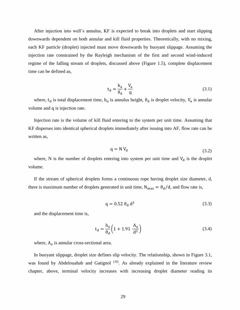
29
After injection into well’s annulus, KF is expected to break into droplets and start slipping
downwards dependent on both annular and kill fluid properties. Theoretically, with no mixing,
each KF particle (droplet) injected must move downwards by buoyant slippage. Assuming the
injection rate constrained by the Rayleigh mechanism of the first and second wind-induced
regime of the falling stream of droplets, discussed above (Figure 1.5), complete displacement
time can be defined as,
td =
haϑd+Vaq
(3.1)
where, td is total displacement time, ha is annulus height, ϑd is droplet velocity, Va is annular
volume and q is injection rate.
Injection rate is the volume of kill fluid entering to the system per unit time. Assuming that
KF disperses into identical spherical droplets immediately after issuing into AF, flow rate can be
written as,
q = N Vd (3.2)
where, N is the number of droplets entering into system per unit time and Vd is the droplet
volume.
If the stream of spherical droplets forms a continuous rope having droplet size diameter, d,
there is maximum number of droplets generated in unit time, Nmax = ϑd d⁄ , and flow rate is,
q = 0.52 ϑd d2 (3.3)
and the displacement time is,
td =haϑd(1 + 1.91
Aa d2
) (3.4)
where, Aa is annular cross-sectional area.
In buoyant slippage, droplet size defines slip velocity. The relationship, shown in Figure 3.1,
was found by Abdelouahab and Gatignol [29]. As already explained in the literature review
chapter, above, terminal velocity increases with increasing droplet diameter reading its

30
maximum value. For larger sizes of droplets, velocity would reduce until it becomes independent
from droplet size.
Figure 3.1: Terminal velocity vs. size of fluid droplets [28]
The authors proposed the following formula of velocity for Part A – velocity increase with
droplet size as,
ϑA = ϑL [1 + (82 mp μf
ρf αp ϑL d)
2
]
1 2⁄
⁄ (3.5)
where lift velocity, ϑL, is,
ϑL = 2(σg∆ρ ρ𝑓2⁄ )1 4⁄
(3.6)
and dimensionless fit factor, mp, for peak velocity is,
mp =ρf ϑL82 μf
dp√1 − αp2 (3.7)
and the ratio of velocities for peak velocity, αp, is,
αp = 1/ [1 + (17.58μfϑLσ)1 2⁄
]
1 2⁄
(3.8)
In order to compute maximum velocity from Equation 3.5 they proposed peak diameter
formula as,
dp = 1.311(σ g ∆ρ⁄ )1 2⁄ (3.9)

31
The authors also proposed velocity formula for Part B – velocity decrease with droplet size as,
ϑB = [
g ∆ρ
2 αp ρfd +
4 αp σ
d ρf]
1 2⁄
(3.10)
In order to limit the size a maximum stable droplet diameter from Clift and Weber [30] is used,
dmax ≈ 4(σ g∆ρ⁄ )1 2⁄ (3.11)
where, σ is interfacial tension of fluids, ∆ρ is density difference between fluids, ρf is stagnant
fluid density, μf is stagnant fluid viscosity and d is equivalent droplet diameter.
The above model is used to derive the minimum displacement time equation as,
tdA =1
60 haϑA (1 + 1.91
Aa d2
) for 0 < d < dp (Part A) (3.12)
and,
tdB =1
60
haϑB(1 + 1.91
Aa d2
) for dp < d < dmax (Part B) (3.13)
As shown in Appendix-A, substituting explicit expressions for ϑA and ϑB gives two formulas
for displacement time:
tdA =ha
120 b √1 +
a
d2 (1 + 1.91
Aa d2
) for 0 < d < dp
and,
tdB =1
60
hac √d
√e d2 + f(1 + 1.91
Aa d2
) for dp < d < dmax
As proved in Appendix-A, the minimum displacement time is for the maximum droplet size,
i.e. maximum terminal velocity. Abdelouahab and Gatignol [29] stated the alpha peak value of 24
ppg bromoform as 0.871 and interfacial tension value as 40.6 dynes/cm. The same kill fluid
displacing a 9 ppg fluid in a 3000-foot annulus (9 in – 7 in casings, Aa=0.174 sqft ) is plotted in
Figure 3.2.
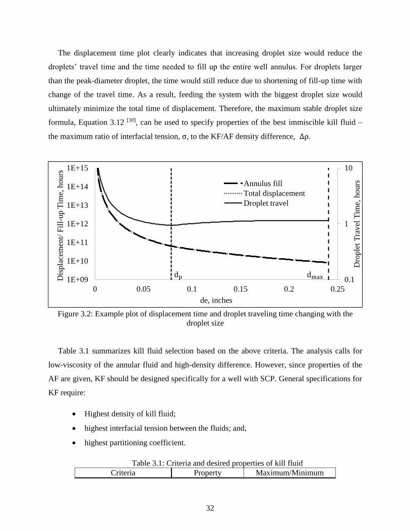
32
The displacement time plot clearly indicates that increasing droplet size would reduce the
droplets’ travel time and the time needed to fill up the entire well annulus. For droplets larger
than the peak-diameter droplet, the time would still reduce due to shortening of fill-up time with
change of the travel time. As a result, feeding the system with the biggest droplet size would
ultimately minimize the total time of displacement. Therefore, the maximum stable droplet size
formula, Equation 3.12 [30], can be used to specify properties of the best immiscible kill fluid –
the maximum ratio of interfacial tension, σ, to the KF/AF density difference, ∆ρ.
Figure 3.2: Example plot of displacement time and droplet traveling time changing with the
droplet size
Table 3.1 summarizes kill fluid selection based on the above criteria. The analysis calls for
low-viscosity of the annular fluid and high-density difference. However, since properties of the
AF are given, KF should be designed specifically for a well with SCP. General specifications for
KF require:
Highest density of kill fluid;
highest interfacial tension between the fluids; and,
highest partitioning coefficient.
Table 3.1: Criteria and desired properties of kill fluid
Criteria Property Maximum/Minimum
0.1
1
10
1E+09
1E+10
1E+11
1E+12
1E+13
1E+14
1E+15
0 0.05 0.1 0.15 0.2 0.25
Dro
ple
t T
ravel
Tim
e, h
ou
rs
Dis
pla
cem
ent/
Fil
l-up T
ime,
hours
de, inches
Annulus fill
Total displacement
Droplet travel
dp dmax

33
Pressure Replacement ∆ρ = ρkf − ρaf Maximum
Buoyancy ∆ρ μaf⁄ Maximum
Immiscibility log(P) Maximum
Displacement time
(Stable droplet size) σ ∆ρ⁄ Maximum
Fluids having the specified properties are available in the market; for instance, Abdelouahab
and Gatignol [29] used bromoform, which is a derivative of bromine (Br), that has a specific
gravity of 2.85 and is highly hydrophobic. However, these general properties are not sufficient
for field use. Other specifications such as toxicity and corrosion rate (over 1 mm/year) make
bromine a poor selection. Injecting a toxic and corrosive material in an annulus would result in
failure of casings and might lead to environmental hazards. Another material called
perchloroethylene, which is a kind of chlorocarbon, is a chemical being used for dry cleaning of
fabrics. It appears to be less toxic and less corrosive as compared to bromine, while; its specific
gravity can go up to 1.609. This liquid could be potentially used for remediating wells with low
SCP, so, its applications would be limited.
Albemarle Brominated Organics
Albemarle Process Development Center – Bromine Research and Technology Group has
developed fluids considering the selection requirements. They produced brominated organic
liquids that have low viscosity since they are comprised of light atoms such as carbon, hydrogen,
and oxygen and have significantly higher density since bromine is a heavy atom. The densities of
their products can be adjusted between 11 to 25 ppg and the fluids are able to withstand up to at
least 150 degrees Celsius. In addition, their partitioning coefficient values varies from 2 to 7,
which makes the fluids highly hydrophobic. The chemical formula of the product is kept
confidential by Albemarle Corporation due to marketing purposes.
The method Albemarle used for producing kill fluids with different densities was by blending
three main components together; A, B and C with densities of 11.08 ppg, 24.7 ppg and 7.01 ppg,
and viscosities of 4090 cP, 2 cP and 13 cP, respectively. Component B was mainly used for
adding density to the blend and the two other components were used for dilution. Figure 3.3
shows the trend of viscosity with increasing density for the brominated organics produced with

34
components A and B. As can be seen, usage of component A for lowering densities results in
dramatic viscosity increase. Therefore, low viscosity brominated organics were obtained by
using component C.
Figure 3.3: Viscosity versus density of brominated organics blended with components A and B
The brominated organics were chosen as the candidate kill fluids and compatibility tests have
been conducted to evaluate their performance in water-based fluids.
Compatibility Testing of Brominated Organics
Compatibility of the KF and AF is a combination of properties specified in Table 3.1 that
would result in gravity displacement. After selecting a hydrophobic KF, its performance should
be tested in water before any further studies. To do this, a set of basic tests was conducted in
LSU PETRLL and Albemarle labs.
3.4.1 Pilot Demo Test – 1
The first trial observation of brominated organics interacting with water was made by simply
pouring 16 ppg organic solvent into a 4” ODx10 feet close-ended clear-PVC pipe filled with
water to its ¾ height and a pressure gage attached to its bottom. A funnel with one-inch tip was
installed on top of the pipe to direct the kill fluid flow into the pipe. Funnel’s tip was 2 feet
above the water level.
Procedure was to pour 2.5 gallons of kill fluid continuously by also keeping the same liquid
level in the funnel. Therefore the injection rate would be more or less constant due to the
y = 8E+10x-6.98
0
500
1000
1500
2000
2500
3000
3500
4000
10 15 20
Vis
cost
y (
cP)
Density (ppg)

35
continual hydrostatic pressure exerting to the funnel’s tip. Entire process of kill fluid settlement
in water was videotaped and slipping times of droplets were recorded. After the system became
static, settled kill fluid was recovered from the valve at the bottom.
First remark was the stream of kill fluid droplets hitting on the water surface and entrapping
air onto their bodies. As these droplets traveled down, they parted to smaller bodies and attached
air bubbles lifted up particularly the smaller droplets. Ultimately most of the droplets were able
to become bubble-free, however the bottom sedimentation of kill fluid still included air in its
structure. The air eventually migrated while carrying-over some kill fluid droplets upwards and
delayed the static stabilization time of the system. As the water level increased the injection tip
became submerged and eliminated the air entrapment. Slip velocity of a single droplet in water
was then measured as around 43 feet per minute.
In summary, intrusion of the 3rd phase, air, slowed down the settling process so the submerged
injection is required. During the settling process; the pressure value on the gage increased
continuously and at the end; close to 100% of the kill fluid was recovered. No mixing with water
was observed.
3.4.2 Pilot Demo Test – 2
In the light of the learning from the first demo test, a second test was designed and conducted
to see the performance of the brominated organics with submerged injection and w/o trapped air
during the injection. In addition to the same set-up and procedure, a 2 feet pipe with a 3/16”
orifice was attached to the funnel to assure sub-surface injection of kill fluid.
As a result of submerged injection, stabilization time was significantly reduced. Organic
droplets would continuously travel down without interacting with air bubbles. In front of the
orifice, a 2 feet long dynamic jet was observed and at the end of the jet various sizes of droplets
were formed. When jetting forces expired, this jet turned into a buoyant jet and formed droplets
started to move downwards only under buoyant forces. During the injection process, the small
droplets most of the time failed to travel downwards and were either suspended or lifted-up by
the counter-current flow.
36
The velocity of a considerably big droplet being produced by the orifice was this time
measured as around 60 feet per minute, 40% more than in the first test. Therefore, as a
conclusion, if vertical injection is the case; air entrapment must be avoided by assuring a
submerged kill fluid injection.
3.4.3 Weighted Fluid Column Test
A one-time compatibility test by using weighted annular fluid was performed in Albemarle
PDC laboratories. The test was conducted in a vertical 3 feet glass pipe with 1.5” diameter. A 16
ppg brominated organic was dripped into the column of 14.2 ppg colorless calcium bromide
solution. The slipping time was measured.
Observations indicated that the presence of a heavier stagnant medium slows down the
droplets from slipping downwards, as already known from the literature. In addition, it was
observed that low injection flow rate through a circular nozzle provides big droplets with
uniform same size and these droplets can travel to the bottom without any interruption. The
velocity of the droplets slipping in the kill solution was measured as 10-12 feet per minute,
which is, considerably, lower than the velocity in water.
3.4.4 Bench-top Compatibility Tests
Previous compatibility tests involved only Newtonian fluids as the stagnant medium. To find
out the performance of brominated organics in Non-Newtonian fluids, several bench-scale tests
were performed in Albemarle PDC laboratories.
A custom made glass model, shown in Figure 3.4, was designed such that two glass pipes
with diameters of 2” and 4” would be attached in another to form a 1” width of annular gap.
Total length was 3 feet and the volumetric capacity was 1.5 gallons. The injection would take
place in the annulus by using either a 0.25” glass funnel or nitrogen source feeding a 0.125”
tygon tubing, and the annulus of the model would be drained from the valve at the bottom. In the
tests, two kill fluids blended using components A and B are used, with densities of 15.4 ppg
(orange) and 24.8 ppg (blue) and viscosities of 500 cP and 8 cP, respectively. And translucent
annular fluids with a rheology character of Yield-Power-Law with high viscosity and 8.5 ppg
density. Kill fluids were injected into the column by either pouring from a funnel or transferring
pressure from the nitrogen bottle. The limited pressure source did not allow high flow rates for

37
the viscous kill fluid. Nevertheless, for the low viscosity organic three different flow rates could
be obtained. In the tests, ¾ of the column (~1 gal) was filled with AF, and continuous submerged
injection of KF was performed. Whole phenomenon was captured by a video camera.
Figure 3.4: Bench-top physical model for compatibility tests
Results showed that when the injection rate is too high (Figure 3.5 - right picture), kill fluid
disperses into the annular fluid and spreads throughout the AF column. However, when the rate
is low (Figure 3.5 - left picture) uniform droplets form and settle down, reach the bottom and
build-up. The phenomenon, as discussed above in the literature review chapter, is defined by the
fragmentation modes directly influenced by the injection rate. Rayleigh mechanism, which
causes big uniform droplets, is possible with low rates and enables an unconstraint transport of
KF. Atomization regime causes mixture (due to dispersion) at the top and forms small KF
droplets that fail to travel down but upwards. When Atomization is avoided a mixture zone forms
at the KF/AF interface (at the bottom) due to disturbance that caused by the settling KF droplets.
Formation of this zone begins at the very bottom and expands as the KF feed continues. Figure
3.6 shows the amount of mixture when the same amount of KF was injected in the same AF with
different flow rates. For the lowest injection rate, mixture zone is comparably smaller than that
with the highest.
2” Glass tube
4” Glass tube
Nitrogen Bottle
0.125” Tygon
tubing
3 feet
Drainage

38
Figure 3.5: Bench-top compatibility tests; (0.11, 0.28, 0.57 gpm) Flow patterns vary from
Rayleigh to Atomization.
Figure 3.6: Snapshots of the tests when injection stopped. Mixture zone height increased with
increasing injection rate.

39
In addition to forced injections (with controlled rate), few funnel experiments (free fluid
discharge from funnel) were conducted by using different kill fluids. As seen in Figure 3.7, low
viscosity-high density kill fluids showed different fragmentation modes (as already shown in
Figure 1.5) and therefore caused various sizes of mixture zones; although, high viscosity- low
density fluid performed a slow consistent slippage and generated no mixture zone. Unfortunately
injection rate was limited for high viscosity fluid and its behavior under forced injection could
not be observed.
In summary, kill fluid viscosity (not specified in Table 3.1) is an important property that
controls dispersion and formation of mixture zone. Even though the heaviest fluid with low
viscosity travels to the bottom much faster, generation of a mixture zone reduces the process
performance. Instead of settling part of KF remains suspended. Thus, a fully compatible KF with
high density should also feature elevated viscosity.
Figure 3.7: Poured kill fluids into Non-Newtonian AF generate different flow patterns. Left: Low
viscosity kill-fluid with Rayleigh mechanism. Middle: High viscosity kill-fluid with First-
Induced break-up. Right: Second-Induced Break-up [14].
40
Summary
Brominated organic fluids have been developed by Albemarle Corporation and tested for
compatibility with water and synthetic clay suspensions. The demo tests with water mainly
provided information about the injection method. Evidently, dumbing the kill fluid above free
AF surface results in air entrapment and slows down the settling process (For well applications,
this might even cause taking the kill fluid back during the bleed-off cycles). To avoid this
negative effect, submerged injection was conducted in all other tests.
Bench-top tests showed relation of droplet size being highly dependent on the injection rate.
Highest rate caused partial dispersion of kill fluid in the annular fluids in small droplets and
decreased settling of the kill fluid to the bottom.
Brominated organics provide flexibility in combinations of density, viscosity and interfacial
tension. They are a promising kill fluid to be used in gravity displacement of annular fluid.
However, operational parameters must carefully be designed.

41
CHAPTER 4: VISUALIZATION OF GRAVITY DISPLACEMENT
Objective
As discussed above, in the past, the bleed-and-lube technique for SCP removal by placing
heavy fluid (KF) on the top of annular cement to kill gas migration has been tried and failed
because the kill fluid did not effectively displaced the annular fluid column above the cement
top. As the displacement requires gravity settling of the kill fluid in the lighter annular fluid,
there was a need for a laboratory visualization model to study and understand the mechanism of
the displacement process.
The first objective was to fabricate transparent laboratory scaled-down hydraulic analog of
well’s annulus. The second objective was to formulate clear synthetic-clay muds. The third
objective was to conduct series of experiments with various kill fluids injected at the top and at
the side of the annulus filled with different muds until maximum displacement occurred. The
results involve videotapes, pressure records and measured volumes of the kill fluids. The
measurements provide assessment of the process performance while the videos were used for
geometrical description of the kill fluid plume change on its way down the annulus.
The following aspects of the displacement process are tested in this study:
Comparison of the top with side injection in terms of fluid slippage and its consistency.
Effect of the two fluids properties on fluid mixing and the slippage
Comparison of immiscible and miscible injection
Design of operational parameters for efficient injection of kill fluid
Methodology
4.2.1 Physical Model Design and Fabrication
Physical simulation of an annulus is a difficult task. Even though the design of circular pipes
is alike to that of a well, they have significant disadvantages such as the visualization and
disassembling practicality. A bench-top physical model, dubbed here “slot model”, has been
designed by opening up the annulus to the sides and obtaining a rectangular geometry (Figure
4.1)

42
Figure 4.1: Well annulus (left) was cut from the red line; opened-up and converted into Slot
model (right).
The easiest way of calculating the flow characteristics in a non-circular conduit is to compare
it with a circular pipe, which is possible by calculating the shape’s “equivalent diameter”[66].
Langlinais et al. [67] used this approach to calculate the frictional pressure losses in a drill pipe
annulus but the method has never been used for buoyant displacement studies. The concept has
been employed to the slot model in order to maintain the hydraulic similarity of shapes, annulus
and the slot.
Hydraulic radius, which is defined as the ratio of the shape’s cross-sectional area to its
wetting perimeter, is widely being used under the name of equivalent diameter (de=4rH)[68].
Equating the hydraulic radiuses of both shapes gives the following mathematical relationship.
rHannulus = rHslot = rH (4.1)
Considering,
rH =w ∆d
2(w + ∆d)
Gives,
w =
2 rH ∆d
∆d − 2 rH (4.2)
Figure 4.2 shows the plot of Equation 4.2. As it is shown, hydraulic diameter defines both the
vertical and horizontal asymptotes. Sixty-two different combinations of casings are first
considered and hydraulic radii of these combinations are calculated. To limit the population with
the intermediate annuluses that generate SCP conductor casings, surface casings and relatively
w
∆d

43
small production casings are excluded, and 40 intermediate casings between 13 3/8” and 5” are
taken into consideration and hydraulic radii of each are calculated (Table 4.1).
Figure 4.2: Dimensions plot for the slot model according to hydraulic radius theory
Statistical analysis of a population of 40 hydraulic radiuses gives right-skewed distribution
and is shown in Figure 4.3. Statistical properties and results are also given in Table 4.2 and Table
4.3. Figure 4.4 shows the plots of the slot model width versus thickness for different central
tendency measures of annuluses. The selected design was 1.3” thick and 20” wide slot that was
later changed to 1.35” and 13.5”, respectively, due to fabrication constraints.
Figure 4.3: Statistical analysis of hydraulic radius of 40 intermediate casings
w
∆𝑑
vertical asymptot
horizontal asymptot
0%
27.5%
65%
87.5%97.5% 100%
0%
20%
40%
60%
80%
100%
0
2
4
6
8
10
12
14
16
0.28 0.45 0.61 0.78 0.94 1.11 1.27
% C
um
ula
tive
Fre
quen
cy
# o
f occ
urr
ence
Hydraulic radius, in
Number of
occurance
%Cumulative
frequency
(rH, rH)

44
Table 4.1: Table of hydraulic radiuses for various casings and annular areas (OC= Outer casing,
IC= Inner casing, ID= Inner diameter, OD= Outer diameter, NW= nominal weight [lb/ft.], CS=
Cross-Section, rh = Hydraulic Radius)
OC
OD, in
OC
NW
in
OC
Thickness
in
OC ID
in
OC Drift
diameter
in
Bit
size
in
Clearance
in
IC
OD
in
CS
Area
sqin
Wetting
Perimeter
in
rh
in
13.375 48 0.33 12.715 12.559 12.25 0.1545 9.625 54.22 70.18 0.773
13.375 54.5 0.38 12.615 12.459 12.25 0.1045 9.625 52.23 69.87 0.748
12.615 12.459 12.25 0.1045 8.625 66.56 66.73 0.998
13.375 61 0.43 12.515 12.359 12.25 0.0545 9.625 50.25 69.55 0.723
12.515 12.359 12.25 0.0545 8.625 64.59 66.41 0.973
13.375 68 0.48 12.415 12.259 12.25 0.0045 9.625 48.30 69.24 0.698
12.415 12.259 12.25 0.0045 8.625 62.63 66.10 0.948
13.375 72 0.514 12.347 12.191 11 0.5955 8.625 61.31 65.89 0.931
12.347 12.191 11 0.5955 7.625 74.07 62.74 1.181
10.75 51 0.45 9.85 9.694 9.5 0.097 7 37.72 52.94 0.713
10.75 55 0.495 9.76 9.604 9.5 0.052 7 36.33 52.65 0.690
10.75 60.7 0.545 9.66 9.504 9.5 0.002 7 34.81 52.34 0.665
10.75 65.7 0.595 9.56 9.404 8.75 0.327 7 33.30 52.02 0.640
9.56 9.404 8.75 0.327 6.625 37.31 50.85 0.734
9.625 32.3 0.312 9.001 8.845 8.75 0.0475 7 25.15 50.27 0.500
9.001 8.845 8.75 0.0475 6.625 29.16 49.09 0.594
9.625 36 0.352 8.921 8.765 8.75 0.0075 7 24.02 50.02 0.480
8.921 8.765 8.75 0.0075 6.625 28.03 48.84 0.574
9.625 40 0.395 8.835 8.679 8.625 0.027 7 22.82 49.75 0.459
8.835 8.679 8.625 0.027 6.625 26.83 48.57 0.553
9.625 43.5 0.435 8.755 8.599 8.5 0.0495 6.625 25.73 48.32 0.533
8.755 8.599 8.5 0.0495 6 31.93 46.35 0.689
9.625 47 0.472 8.681 8.525 8.5 0.0125 6.625 24.72 48.09 0.514
8.681 8.525 8.5 0.0125 6 30.91 46.12 0.670
9.625 53.5 0.545 8.535 8.379 8.375 0.002 6 28.94 45.66 0.634
8.535 8.379 8.375 0.002 5.5 33.45 44.09 0.759
8.625 24 0.264 8.097 7.972 7.875 0.0485 6 23.22 44.29 0.524
8.097 7.972 7.875 0.0485 5.5 27.73 42.72 0.649
8.625 28 0.304 8.017 7.892 7.875 0.0085 6 22.21 44.04 0.504
8.017 7.892 7.875 0.0085 5.5 26.72 42.46 0.629
8.625 32 0.352 7.921 7.796 6.75 0.523 5 29.64 40.59 0.730
8.625 36 0.4 7.825 7.7 6.75 0.475 5 28.46 40.29 0.706
8.625 40 0.45 7.725 7.6 6.75 0.425 5 27.23 39.98 0.681
8.625 44 0.5 7.625 7.5 6.75 0.375 5 26.03 39.66 0.656
8.625 49 0.557 7.511 7.386 6.75 0.318 5 24.67 39.30 0.628
7.625 24 0.3 7.025 6.9 6.75 0.075 5 19.12 37.78 0.506
7.625 26.4 0.328 6.969 6.844 6.75 0.047 5 18.51 37.60 0.492
7.625 29.7 0.375 6.875 6.75 6.75 0 5 17.49 37.31 0.469
7.625 33.7 0.43 6.765 6.64 6.5 0.07 5 16.31 36.96 0.441
7.625 39 0.5 6.625 6.5 6.5 0 5 14.84 36.52 0.406

45
Table 4.2: Statistical results of annulus hydraulic diameters
rH # of
occurrence
Relative
Frequency %frequency
Cumulative
Frequency
%Cumulative
frequency
0.2 to 0.365 0 0.000 0.00 % 0.00 0.00%
0.365 to 0.53 11 0.275 27.50 % 11.00 27.50 %
0.53 to 0.695 15 0.375 37.50 % 26.00 65.00 %
0.695 to 0.86 9 0.225 22.50 % 35.00 87.50 %
0.86 to 1.025 4 0.100 10.00 % 39.00 97.50 %
1.025 to 1.19 1 0.025 2.50 % 40.00 100.00 %
1.19 to 1.355 0 0.000 0.00 % 40.00 100.00 %
Totals 40 1 100 %
Table 4.3: Statistical properties of annulus hydraulic diameters
Count 40 # of classes 5 P90 0.82
Max Value 1.181 Class Width 0.165 P10 0.35
Min Value 0.459 Average 0.66
Range 0.722 Median 0.653
Figure 4.4: Slow model width vs. thickness plotted according to statistical results.
The model has been fabricated in LSU using one 0.75” thick glass for the front sight and a
chemically resistant plastic plate for the back plate. The whole system was sealed with durable
rubber and c-clamps. Injection could be conducted from nozzles with different sizes (0.125”,
0.5”, 0.6”), located at either at the top of the model or at the rear center point, below the top.
Overflowing fluid could be collected from 1” holes drilled to the sides of the plastic plates one
inch below the top that were connected to flexible hoses. A Teflon single cavity ½ HP motor
pump is used for the injection and a pressure transducer is installed at the bottom drainage line to
read the bottom pressure changes. Fluid displacement process in the model could be seen and
0
2
4
6
8
10
12
14
16
1 1.5 2 2.5 3
w, in
delta(d), in
AverageP90MedianP50

46
recorded with a video camera placed in front of the glass window. The volume of the model was
designed as 2.8 gallons however due to plastic sealant rubber and clamping method the volume
could be between 2.5 to 3 gallons. Schematics of the model is shown in Figure 4.5.
Figure 4.5: Slot physical model schematics
4.2.2 Fluids Properties
To conduct the displacement experiments, different kill fluids (KF) with various properties
are used. Table 4.4 shows the kill fluids named according to their densities and viscosities. KF
starting with #1 represents brominated organic fluids; #2 is weighted drilling mud and #3 shows
heavy brine. Due to the available amount of KF1701, most of the experiments are conducted
with it. Initial injection experiments with water as the annular fluids have been visually
informing; however, according to characterization of annular fluid studies, fluid in a well
13.5 in Flow
Meter Side
injection
KF
KF Tank Pump
Pressure
Transducer
3 ft.
AF
overflow
Top
injection
KF
KF
Drain

47
annulus – underneath the water layer – is expected to be a Non-Newtonian fluid that shows
structural strength. Structural strength defined in this work as a combination of high rheology
(viscosity) and tixotrophy (gel strength). For tixotrophy Laponite ® - a synthetic-based clay – is
mixed with water, and for viscosity cellulose derivatives, PAC or Xantham Gum, are used. These
fluids could also be weighted-up with Potassium Formate salt; however, this resulted in loss of
structural strength.
Table 4.4: Kill fluid properties used in slot experiments
Density,
ppg
Viscosity,
cP
Estimated IFT
dyne/cm Material
KF1201 11.95 14 30 Organic
KF1202 11.95 54 30 Organic
KF1203 11.95 94 30 Organic
KF1204 11.85 8 32 Organic
KF1401 13.9 11 30 Organic
KF1601 15.8 11 30 Organic
KF1402 14.1 25 30 Organic
KF1701 16.68 235 21.5 Organic
KF2012 12
Mud
KF2013 13.5
Mud
KF3011 11.25
Brine
Formulas of the translucent fluids is shown in Table 4.5, and rheology comparison of
translucent fluids and un-weighted bentonite muds are in Figure 4.6. Higher Laponite
concentrations gave higher gel strength values up to 30 lbf./100sqft. The hydration time of
Laponite was tested as 5 days [45]. Thereby, fluids to be used for the slot experiments were mixed
3-5 fold greater than model capacity at least 5 days before the tests. Translucent fluids’ rheology
was computed (Table 4.6) from Fann-vg viscometer readings at 3 and 100 rpm using the
following formulas for plastic viscosity,
μLow Shear =300
100 − 3(θ100 − θ3)
And for the yield point,
τ0 = θ3 − μLow Shear 3
300

48
Figure 4.6: Comparison of two translucent fluids and un-weighted bentonite muds
Table 4.5: Prepared translucent fluid formulas for slot model experiments
Grams of product per 350 mL water (lb/bbl.)
Name Laponite Pac Xantham Gum
TF0101 1.1 0.03
TF0102
1.75
TF0103 1.65 0.06 0
TF0104
0.9
TF0105 2.5 0.1
TF0107 2 1
TF0108 0.02
TF0205
1
TF0206 4 1
TF0207 2 1
TF0208
1
Table 4.6: Properties of generated translucent fluids for slot experiments
TF
0101
TF
0102
TF
0103
TF
0104
TF
0105
TF
0107
TF
0108
TF
0205
TF
0206
TF
0207
TF
0208
Density (ppg) 8.4 8.4 8.4 8.4 8.4 8.4 8.4 11 9.6 10 10
Low shear
viscosity (cP) 12.4 24.7 18.6 17 24.7 40.2 21.7 26.3 29.4 15.5 15.5
Yield Point
(lbf/100sqft) 0.9 9.8 1.8 3.8 10.8 6.6 0.8 2.2 2.7 1.9 0.9
10 min Gel
(lbf/100sqft) 11 11 20 7 32 30 1.5 6 5 3 2
0
5
10
15
20
25
0 100 200 300 400 500 600
Shea
r S
tres
s, l
bf/
100sq
ft
Shear Rate, RPM
TF0101
TF0103
15 ppb bentonite mud
20 ppb bentonite mud

49
4.2.3 Experimental Procedure and Analysis
Experimental procedure consisted of five parts.
1. Prepare sample of TF and measure rheology and gel strength.
2. Fill up the slot model with TF from the top
3. Inject KF into the slot model from the top/side port using desired nozzle size and at the
designed constant flow rate until bottom pressure stabilizes.
4. When bottom pressure does not increase for at least a minute (or no more kill fluid is
available); stop injection
5. Videotape the whole experimental run
Visual record and pressure data were obtained during the experiments. In order to explain the
phenomenon clearly, geometry of the process is evaluated. The impingement widths (W) and
impingement heights (h) of each side injection run is measured. For the top injection droplet
fragmentations are visually inspected and evaluated according to the study of Reitz [14], as
already explain in Figure 1.5 in the literature review chapter of this work.
Beside the qualitative visual study of videos, quantitative inspection of bottom pressure is also
evaluated. Recorded pressure data and injected KF volume are converted into dimensionless
relationships of pressure replacement efficiency (Ep) and displacement ratio (R) defined as,
Ep =
∆P
∆Pu=P − PiPu − Pi
(4.3)
R =
Vp
Vs (4.4)
where, P is the bottom pressure, Pi is the initial bottom pressure when the model is filled with
only AF, Pu is the ultimate bottom pressure when the model is filled with only KF, ∆P is the
change in bottom pressure, ∆Pu is the pressure difference when AF is completely replaced with
the KF, Vp is the volume of KF pumped into the model, and Vs is the slot model volume.
Results and discussion
A total of 59 experiments were conducted using various combinations of annular and kill
fluids at different flow rates. For viscous kill fluids – particularly KF1701 and heavy muds –

50
flow rate was limited by the pump. The results are shown in Table 4.7; where, KF refers to kill
fluid and TF refers to translucent fluid. In the table, nozzle sizes (dn) and direction of injection
are also stated. For the patterns; “GF” is gravity flow, Rayleigh is Rayleigh break-up regime and
“Atom” stands for atomization regime[69]. There were two above surface injections that are
shown in the table with “as” addition. Flow rates are varied between 0.5 gpm to 5 gpm; however,
due to the manual flow meter, these numbers may show +- 5% error.
Table 4.7: Table of results No KF TF q, gpm side/top dn, in W, in h, in pattern
1 1201 0101 2 side 0.5 3.32 2.6 GF
2 1201 0101 5 side 0.5 4.8 2.7 GF
3 1202 0103 0.5 side 0.5 0 0 Rayleigh
4 1202 0103 2 side 0.5 2.4 9.6 Rivulet
5 1202 0103 5 side 0.5 4.4 6.8 GF
6 1203 0101 0.75 side 0.5 0 2.7 Rayleigh
7 1203 0101 2 side 0.5 2.6 5.5 GF
8 1203 0101 5 side 0.5 3.4 5.5 GF
9 1401 0103 1 side 0.25 2 4 GF
10 1401 0103 2 side 0.25 4.1 4 GF
11 1401 0104 1 side 0.5 0 0 Rayleigh
12 1401 0104 2 side 0.5 2.36 3.5 GF
13 1401 0104 5 side 0.5 5.9 3.5 GF
14 1201 0101 1 top 0.5 0 2.7 Rayleigh
15 1201 0101 0.5 top 0.5 0 2.7 Rayleigh
16 1201 0101 5 top 0.5 0 4 Atom
17 1201 0102 2 top 0.5 0 2 Rayleigh
18 1201 0102 5 top 0.5 0 1 Atom
19 1202 0103 2 top 0.5 0 5.5 Induced
20 1203 0101 0.5 top 0.5 0 1.3 Rayleigh
21 1203 0101 5 top 0.5 0 5.8 Atom
22 1401 0103 1 top 0.25 0 4.6 Induced
23 1401 0104 1 top 0.5 0 4.6 Rayleigh
24 1401 0104 2 top 0.5 0 4.6 Induced
25 1401 0104 5 top 0.5 0 9 Atom
26 1204 0104 3 side 0.5 6.9 7.6 GF
27 1204 0104 3 top 0.6 0 10.7 Atom
28 1401 0104 3 side 0.5 5.17 7.65 GF
29 1402 0206 2 side 0.5 4.1 5.47 GF
30 1204 0107 2 side 0.4 8.7 11.9 GF
31 1204 0107 0.5 side 0.4 0 1 Rayleigh
32 1701 0102 2 side 0.6 0.7 11 Rivulet
33 1701 0104 2 side 0.6 3.2 10 GF
34 1701 0107 2 side 0.6 2.5 15.7 Rivulet
35 1701 0107 2 side 0.6 3 13 GF
36 1701 0107 0.5 side 0.6 0 4.3 Rayleigh

51
Table 4.7 continued
37 1701 0107 1.5 side 0.6 0.8 11.35 Rivulet
38 1701 0207 1.5 side 0.6 3.5 13.4 GF
39 1701 0208 1.5 side 0.6 3.13 13.45 GF
40 1701 0208 2 side 0.6 4 13.45 GF
41 1701 0107 5 side 1 3.4 15 GF
42 1701 0107 1.5 top 0.6 0 12.4 Induced
43 1701 0107 0.5 top 0.6 0 8.3 Rayleigh
44 1701 0107 1.5 top 0.125 0 0 Atom
45 1701 water 1.5 side 0.6 2.9 13.45 GF
46 1701 water 2 side 0.6 3.4 13.45 GF
47 1701 0107 1 side (as) 1 1.47 Rivulet
48 2013 0107 1 side 0.6 1.9 15.6 Rivulet
49 2013 0102 2 side 0.6 3.12 18.72 Rivulet
50 2013 0103 2 side 0.6 0 0 0
51 2013 0107 2 side 0.6 5.95 20.6 GF
52 2013 0107 4 side 0.6 7.04 20.6 GF
53 2013 0107 1 side 0.6 0.7 14 Rivulet
54 2013 0107 2 side 0.6 4 16 GF
55 2012 water 3 side 0.6 0 0 0
56 2013 B 8.6 2 side 0.6 4.9 9.75 GF
57 3011 B 8.6 1 side 0.6 2.6 10 Rivulet
58 3011 B 8.6 1 side (as) 0.6 2.4 10 Rivulet
59 1701 air 1.5 side 0.6 2.5 - Rivulet *B= bentonite mud
As the mechanism of miscible and immiscible displacement is completely different the results
are analyzed separately for miscible displacement with brine and heavy mud, and immiscible
displacement with brominated organics.
4.3.1 Observations – Miscible Displacement
Miscible displacement experiments with heavy mud as kill fluid were conducted with
bentonite muds weighted up to 12 and 13.5 ppg with barite, using side injection port and 0.6”
nozzle. Figure 4.7 shows the first and the most obvious observation; instant mixing of mud being
injected into water. The rapid mixing occurs at the top and in about 6 seconds heavy mud spreads
throughout the slot model homogenously.
As shown in Figure 4.8, below, when the heavy mud is injected to Non-Newtonian fluid at 1
gpm rate, a rope of heavy mud forms with no mixing until the rope reaches the bottom. At the
time the rope contacts the bottom it gets destabilized into mixture zone that builds upwards
reaching promptly the overflow ports. However when injection rate is higher, destabilization of

52
heavy mud rope occurs earlier. As demonstrated in Figure 4.9, rope forms at the top but branches
on its way down and mixes with the counter-current flowing translucent fluid.
Figure 4.7: Injecting weighted mud KF2012 into water @~1 gpm (miscible displacement).
Instant mixing occurs (Experiment #55).
Figure 4.8: Injecting heavy mud KF2012 into Non-Newtonian TF0107 @~1 gpm (Experiment
#53). Continuous rope transport and delayed mixing occur i.e. rope length = height of the model.

53
Figure 4.9: Injecting heavy mud KF2014 into Non-Newtonian TF0107 @~2 gpm (Experiment
#51). Rope of KF destabilizes before reaching the bottom due to higher injection rate.
Figure 4.10 shows the pressure replacement efficiency plots of miscible displacements. Forty-
five degree line is the perfect displacement line. The curve-linearity of each plot indicates
increasing mixing of the two fluids while the initial slope value represents instant rate of loss of
KF to overflow being 30% of the injection rate for heavy mud-water run. As one model volume
of heavy mud is injected into water loss to overflow approaches to 65%. For heavy mud being
injected into Non-Newtonian fluid, mixing is delayed and departure from perfect displacement
line occurs after about 40% model volumes of model volume is injected. As injection continues,
loss of heavy mud to overflow increases and loss approaches to 24% as one model volume has
been injected. Heavy-mud KF experiment was conducted in a taller pilot column with no
visualization but bottom pressure readings. When 1.6 model volumes (33 gallons) of heavy mud
was injected, bottom pressure reached the complete displacement (Ep=1). Additional information
about the run is shown in Appendix C.
As stated by Frigaard and Crawshaw [9], high yield stress of mud is required to provide
cement plug slippage as an interface between two Bingham fluids (cement slurry and mud) in a
closed pipe. The visual findings from the heavy mud miscible displacement experiments validate
this statement. In addition, when the mud was pumped slow (Figure 4.8), the stability of the mud

54
stream did not break until it reaches the bottom; however, higher flow rates (Figure 4.9) showed
formation of a slump. This phenomenon is explained by Alba et al. [70] as the exchange flow
determined by the balance between yield stress and buoyant forces when the heavy fluid is
presented into the system instantly.
Figure 4.10: Dimensionless plots of miscible displacement @1 gpm. Miscible kill fluids give
poor displacement of water or water-based Bingham fluid.
Addition series of miscible displacement experiments used heavy brine and water-based
annular fluid. Published LSU tests with heavy brine kill fluids reported rapid flocculation of
annular fluid being the reason for poor displacement[8]. Unlike bentonite muds, Laponite clay
suspensions show no significant flocculation when mixed with brine. Thereby, heavy brine
miscible displacement experiments were conducted in un-weighted bentonite mud with poor
visual inspection.
Injection of 11.25 ppg dyed (red) brine into 8.6 ppg bentonite mud at 1 gpm rate gives similar
displacement performance to that for heavy mud KF and TF0107. Figure 4.11 shows the visual
records of the injection process. Impinging brine slips down as a rope and displaces the mud
(brown). After about 2.5 minutes the model – including the bottom section – becomes red. Visual
inspections indicate that the falling rope of brine creates an envelope of flocculated mud that acts
as a protective coating. The mechanism is demonstrated in Figure 4.14 more clearly. Similar to
heavy mud KF displacement, once the rope reaches the bottom the “coated” rope gets
destabilized and starts building up a mixture zone (MZ). As shown in Figure 4.10, plot of brine
into mud shows a wavy increase due to overflowing slugs of flocculants.
0
0.2
0.4
0.6
0.8
1
0 0.2 0.4 0.6 0.8 1
E
R
Perfect displacement
Brine into mud
Heavy-mud into Laponite

55
Figure 4.11: KF3011 (brine - red) into 8.6 ppg un-weighted mud (brown) with 1 gpm flow rate
(Experiment #57). A flocculated mud coating covered the brine stream as it went down and
displaced the clean mud.
Figure 4.12: Mechanism of heavy brine slippage in mud
4.3.2 Observations – Immiscible Displacement
Hydrophobic fluids do not mix but may break-up while moving downwards under buoyant
forces when injected into a lighter fluid. Therefore, the physics of immiscible displacement is
MZ=KF+AF
Injection
nozzle
Heavy brine
rope Flocculated brine/mud
coating
Injection
(Impingement)
Heavy Brine
(Red)
Flocculated
Drilling mud

56
entirely different from miscible displacement. The geometry and rate of injection may control the
initial consistency and integrity of the KF stream falling downwards. Also, fluid properties, such
as density, interfacial tension and viscosity may affect the final shape and size of the fluid
particles and, therefore, the slippage velocity and displacement rate. Nevertheless, the slot model
experiments could only address the first issue – initial conditions of the displacement process-
the model’s height is too small for studying the second issue.
Injection geometry effect:
Of the two geometries of KF injection conducted, vertical injection is supposed to produce
initial laminar jet that would later destabilize into a droplets, shown in the right side of Figure
4.13. As the KF slippage continues, the droplets settle down at the bottom without mixing.
However, small droplets show very slow or no settling as they get carried upwards by the
displaced fluid and are mostly discharged in overflow.
Figure 4.13: Heavy KF1701 displacing high-strength TF0107 (2 gpm) using side (left) and top
(right) injection geometries
Side injection of KF forms an impingement zone on the glass plate. Size of this zone is much
bigger than the top injection jet size so more KF volume may move downwards as a continuous
stream. Eventually the stream breaks into KF fragments that settle to the bottom with no mixing
Impingement
Mixture
Jet
Dispersion

57
on lesser number of small fluid particles that could be carried upwards to the overflow. Higher
injection rates demonstrate the difference in displacement physics for two injection geometries
more clearly. As shown in Figure 4.14, although more than one model volume was pumped;
dispersed KF droplets settle down when injection stops. Side injection, on the other hand,
completely fills the model bottoms up and does not establish a settling region at the top (Figure
4.15). In summary, it appears that side injection is superior to top injection as the impingement
stabilizes the KF shearing and increases the rate of buoyant slippage.
Figure 4.14: Top-injection of KF1203 into thin TF0101 at 5 gpm (Experiment #21). Fast
injection “atomizes” KF into dispersed phase that eventually settles down with no stable mixture
zone.
Density differential effect:
As stated by many (Archimedes, Stokes, Dedegil [26] etc.) density differential of heavy
particle and stagnant media directly effects the slip velocity of the particle. The observations
indicate that the slot model slower particles often get carried over by the counter-current flow
and overflow. Figure 4.16 shows plots of immiscible kill fluids with different densities being
injected into TF. All plots demonstrate extended condition of perfect displacement (linear trend)
with mixing (non-linear top section). Plot 2 and 4 were run at the same injection rate but
different densities of KF. It is clearly seen that performance of lighter KF is lower, as its
departure from perfect displacement line is much sooner. The results show the beneficial effect

58
of using KF with maximum possible density. In addition, an increase in density differential (or
KF viscosity) reduces the size of stable impingement zone thus enabling higher injection rates.
Figure 4.15: Side injection of KF1203 into thin TF0101 at 5 gpm (Experiment #8). Impingement
absorbs the injection rate energy. Fluid droplets settle down by buoyancy. No stable mixture
zone is observed.
Figure 4.16: Dimensionless plots of immiscible displacement demonstrate beneficial effect of
high density and detrimental effect of high injection rate on performance
0
0.2
0.4
0.6
0.8
1
0 0.2 0.4 0.6 0.8 1
E
R
KF1701 into TF0107 @ 2 gpm (1)
KF1401 into TF0104 @ 3 gpm (2)
KF1204 into TF0107 @ 2 gpm (3)
KF1204 into TF0104 @ 3 gpm (4)

59
Annular fluid strength effect:
In this section, annular fluid’s viscosity and gels are considered together since both properties
are mutually dependent. As can be seen from the comparison between 2 seconds snapshots of
experiments #33 (Figure 4.17) and #32 (Figure 4.18), higher strength of annular fluid caused a
slower transport of kill fluid thus enabling larger mixture zones. Moreover, higher viscosity of
annular fluid caused more stable impingement zones (rivulet flow type of impingement), as the
low viscosity caused unstable impingement zone (gravity flow) that caused spreading of KF
throughout the model and could be more influenced by the counter-current flow.
Figure 4.17: Side injection of KF1701 into low viscosity TF0104 at 2 gpm (Experiment #33).
There is a sharp TF/KF interface – negligible mixture zone formed.
Injection rate effect:
For the top injection geometry and high rate, turbulent jetting generates dispersion
(atomization) of exiting fluid [69] and returns to the overflow with no gravity settling. Reducing
the injection rate allows formation of elongated buoyant jet that entrains annular fluid while
breaking up into distribution of droplets. However, as the annular (displaced) fluid flows
upwards it lifts small droplets thus creates mixture zone – shown in Figure 4.19. As also shown
in Figure 4.20, only extremely low injection rates (0.5 to 1 gpm) would form Rayleigh fragments
[14], and produce big and uniform droplets that are able to travel downwards and settle at the
bottom with no mixing.

60
Figure 4.18: Side injection of KF1701 into high viscosity TF0102 at 2 gpm (Experiment #32).
High strength of TF generated blurry AF/KF interface – mixture zone formed bottoms up.
Figure 4.19: Top-injecting KF1701 into TF0107 at 1.5 gpm (Experiment #42). Despite low rate,
dynamic jetting causes KF dispersion on its way downwards.

61
Figure 4.20: Top injection of KF1203 into thin TF0101 at 0.75 gpm (Experiment #6). Relatively
large KF droplets form and settle down by buoyancy. A sharp KF/AF interface is observed
For the side injection geometry, energy of fluid stream dissipates in the inner wall’s
impingement where buoyant slippage begins. Stability of the impingement limits the injection
rate as increasing flow rate results in large impingement for a given fluid. As shown in Figure
4.21, extremely slow rates allow a smooth transportation of KF to bottom and create a sharp
KF/AF interface. Higher flow rates, as shown in Figure 4.22, impinges and cause more
disturbance at the KF/AF interface thus resulting in mixture zone formation. Moreover, when
rate is higher (or viscosity of KF is low) impingement regime changes from rivulet to gravity
flow type and KF spreads mainly to the sides. Figure 4.23 demonstrates the unstable
impingement. Generated droplets become more vulnerable to counter-current flow and discharge
with AF.
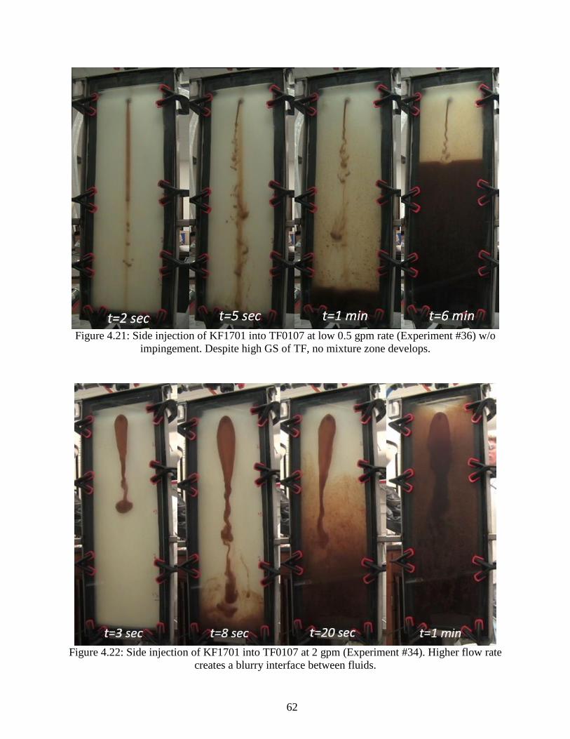
62
Figure 4.21: Side injection of KF1701 into TF0107 at low 0.5 gpm rate (Experiment #36) w/o
impingement. Despite high GS of TF, no mixture zone develops.
Figure 4.22: Side injection of KF1701 into TF0107 at 2 gpm (Experiment #34). Higher flow rate
creates a blurry interface between fluids.

63
Figure 4.23: Side-injection of KF1204 into TF0107 at 2 gpm (Experiment #30) with large
impingement. Low viscosity kill fluid brakes into droplets that are carried upwards by ascending
TF- gravity settling with dispersion.
4.3.3 Relation to Field-Scale Applications
Results of the miscible displacement experiments above show that when the stagnant annular
fluid has no strength the kill fluid (KF) mixes on contact with AF after injection. There is small
(or none) buoyant slippage so fluid displacement in long columns is practically impossible. For
structured AF (with some strength) some initial (rope-type) slippage occurs and mixing might be
merely delayed.
As investigated in the “Characterization of Annular Fluid” chapter in this thesis (Chapter
2.4.2 ), drilling mud in a real well annulus produce water column at the top. This column with no
structure would make it impossible for miscible KF to travel downwards. This may explain the
failure of the early field trials of the Bleed-and-Lube technique with heavy muds [1].
Brominated organics, in the slot model experiments, rapidly settle in water with no mixing.
They also travel through Non-Newtonian (structured) suspension after breaking into large
number of particles (fragments) of various sizes. However, small particles may travel very
slowly or become lifted upwards in the counter-current flow. Counter-current transport occurs
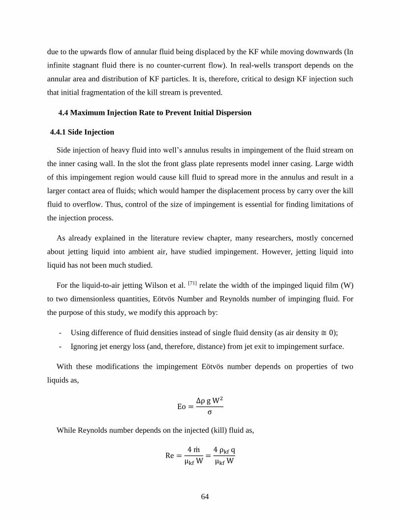
64
due to the upwards flow of annular fluid being displaced by the KF while moving downwards (In
infinite stagnant fluid there is no counter-current flow). In real-wells transport depends on the
annular area and distribution of KF particles. It is, therefore, critical to design KF injection such
that initial fragmentation of the kill stream is prevented.
Maximum Injection Rate to Prevent Initial Dispersion
4.4.1 Side Injection
Side injection of heavy fluid into well’s annulus results in impingement of the fluid stream on
the inner casing wall. In the slot the front glass plate represents model inner casing. Large width
of this impingement region would cause kill fluid to spread more in the annulus and result in a
larger contact area of fluids; which would hamper the displacement process by carry over the kill
fluid to overflow. Thus, control of the size of impingement is essential for finding limitations of
the injection process.
As already explained in the literature review chapter, many researchers, mostly concerned
about jetting liquid into ambient air, have studied impingement. However, jetting liquid into
liquid has not been much studied.
For the liquid-to-air jetting Wilson et al. [71] relate the width of the impinged liquid film (W)
to two dimensionless quantities, Eötvös Number and Reynolds number of impinging fluid. For
the purpose of this study, we modify this approach by:
- Using difference of fluid densities instead of single fluid density (as air density ≅ 0);
- Ignoring jet energy loss (and, therefore, distance) from jet exit to impingement surface.
With these modifications the impingement Eötvös number depends on properties of two
liquids as,
Eo =∆ρ g W2
σ
While Reynolds number depends on the injected (kill) fluid as,
Re =4 m
μkf W=4 ρkf q
μkf W

65
Where, W is the impingement width in inches, ∆ρ is the density differential (ρkf − ρaf) in
ppg., σ is the interfacial tension in dynes/cm, m is the mass flow rate in lb/min, q is the
volumetric flow rate in gal/min and μkf is the kill fluid viscosity in cP.
Wilson et al. [71] defined group parameter, named here as β1 – using our notation – becomes,
β1 =g μkf
4
ρkfσ3
They also combined Eo and Re into another group parameter, β2, as,
β2 =1
16Eo Re2 =
∆ρ g ��2
σ μkf2
And they expressed Eötvös number in terms of the two groups as,
Eo = c12 β1
0.25β20.75
Or,
∆ρ g W2
σ= c1
2 (g μkf
4
ρkfσ3)
0.25
(∆ρ g m2
σ μkf2 )
0.75
where, c1 is the conversion factor and empirical constant.
Solving for W gives formula for impingement size,
W = c1 m0.75
∆ρ0.25μkf0.25 σ0.25
(4.5)
Equation 4.5 is a theoretical formula and needs to be validated. Therefore, the empirical size
from the experiments (Table 4.7) is correlated with that predicted with Equation 4.3 for the
constant “c1” value giving the linear regression slope equal to unity, as shown in Figure 4.24.
The point marked with “x” is excluded from the correlation (Experiment #30). Triangular and
diamond shaped data points represent rivulet and gravity-flow type impingements, respectively.
In some runs, jet forces expired before KF reaching the wall and impingement width became
very small or none. This low injection rate generated Rayleigh fragmentation mode and
considered as rivulet type of impingement due to its desirability.

66
Figure 4.24: Impingement width actual vs prediction plot. Rivulet threshold is estimated as 2.2”
The unit slope regression line gives a=1.904. Therefore, the expression (Equation 4.5)
becomes,
W = 1.904
ρkf0.75 q0.75
∆ρ0.25μkf0.25 σ0.25
(4.6)
The likely reason for poor correlation in Figure 4.24 is that the properties of kill fluids; listed
in Table 4.4, are merely estimates (IFT). Also, measurements of flow rates were not precise.
Nevertheless, the trend in Figure 4.24 is clear. The plot defines threshold between rivulet and
gravity flow type of impingements for the width value, 2.2 inches. Substituting this number to
Equation 4.6 and solving for the injection rate gives the formula for maximum injection rate as,
qcr−i = 1.21 (∆ρ μkf σ)
13
ρkf (4.7)
Equation 4.7 represents the critical rate for impingement criteria. When the injection rate
exceeds this value impingement zone loses its stability and KF droplets spread in the annulus.
0
1
2
3
4
5
6
7
8
9
0 2 4 6 8
W m
easu
red,
inch
es
W predicted, inches
Prediction line
Rivulet
Gravity
Rayleigh
R2=0.57
W=2.2”

67
4.4.2 Top Injection
Reitz [14] studied fragmentation modes of a liquid jet in air[13]. He developed a plot of
Ohnesorge number versus nozzle Reynolds number and defined the threshold conditions (Figure
1.5). (Ohnesorge number relates viscous forces to inertial and surface tension forces) In his
experiments, the ambient fluid was air; however, in this case this fluid is liquid. A Modified
Ohnesorge number, Z, that considers two liquids was proposed by Teng et al. [17]. They used the
Z number for estimation of droplet sizes generated by a liquid spray emerging into an ambient
fluid of different properties. Modified Ohnesorge number in field units is,
Z ≡ 0.018 (3μkf + μaf) (dnσ ρkf)1
2⁄ (4.8)
Using Z instead of Ohnesorge number in estimation of fragmentation modes is theoretically
more accurate; since the effect of annular fluid on displacement process is significant. Figure
4.25, below, is similar to that in Figure 1.5 where Ohnesorge number is replaced with Modified
Ohnesorge number. The transition line formulas in the plot are also modified.
The threshold between transition and atomization mode is,
Z = 948.7 Re−1.25 (4.9)
The threshold between Rayleigh Mechanism and transition is,
Z = 131.9 Re−1.25 (4.10)
As discussed earlier, atomization regime represents the flow pattern when the injected fluid
disperses instantly just after it exits the nozzle. This phenomenon is obviously not wanted for
gravity displacement because small droplets may form emulsion in the countercurrent flow shear
and get lifted upwards. Transition do not atomize; but, generate various sizes of droplets
(satellite droplets [15]) that may be also carried upwards by the displaced liquid. Therefore, flow
rate must be designed such that the flow pattern of the kill fluid jet will always stay below
atomization threshold line in Figure 4.25.

68
Figure 4.25: Fragmentation modes of a liquid jet in pressure atomization into an ambient fluid.
Reynolds number in field units is,
Re = 928 ρkf u dn μkf⁄ (4.11)
Where, ρkf is kill fluid density (ppg), μkf is kill fluid viscosity (cP), u is velocity of the jet
(ft/sec), and dn is nozzle diameter (inches).
Equation 4.10 in field units iss,
Z = 131.9 (
928 ρkf u dnμkf
)−1.25
(4.12)
Velocity of kill fluid in the nozzle is,
u = q An⁄ =4
π
q
dn2
Or in fields units,
u [ft s⁄ ] = 0.41 q dn2⁄ (4.13)
Then, Equation 4.12 becomes,
Z = 0.078 (
ρkf q
μkf dn)−1.25
(4.14)
0.001
0.01
0.1
1
10
1 10 100 1000 10000 100000
Modif
ied O
hnes
org
e N
um
ber
(dim
ensi
on
less
)
Reynolds Number (dimensionless)
Rayleigh Mechanism
Atomization Mode

69
Equation 4.14 defines the modified Ohnesorge number where for offset of transition rate
atomization regime starts forming. Solving for flow rate gives,
0.018(3μkf + μaf)
(dnσ ρkf)12
= 0.078 (ρkf q
μkf dn)−1.25
Or,
qcr−R = 3.23
μkf dn1.4 σ0.4
ρkf0.6(3μkf + μaf)0.8
(4.15)
Equation 4.15 defines critical flow rate to assure the Rayleigh mechanism of jetting. Similar
derivation gives the critical flow rate defining the threshold for atomization,
qcr−A = 15.76
μkf dn1.4 σ0.4
ρkf0.6(3μkf + μaf)0.8
(4.16)
Atomization criteria can be applied to both top and side injection conditions to make sure that
the dynamic forces do not generate the turbulent regime and gravity forces control the jet.
Figure 4.26: Matched flow pattern values for vertical injection
0.001
0.01
0.1
1
10
1.0E+00 1.0E+01 1.0E+02 1.0E+03 1.0E+04 1.0E+05
Modif
ied O
hnes
org
e N
um
ber
Reynolds Number
Calculated
Atomization
Rayleigh
#20 #42
#44

70
Conducted experiments are marked in Reynolds versus Modified Ohnesorge number and
shown in Figure 4.26. The labeled data points are examples of three top jetting modes observed
in our experiments. As shown in Figure 4.27, Rayleigh mechanism allows a continuous transport
of KF to the bottom by maintaining uniform droplets, while atomization mode causes nozzle-
front dispersion and result in inefficient transport.
Figure 4.27: Rayleigh mechanism (left), transition (middle) and atomization modes (left) from
experiments #20, #42 and #44 respectively
As indicated by the power functions in Equation 4.13 and 4.15, the nozzle size has the most
influence on the flow rate. Figure 4.28 illustrates this effect for fluid properties shown in Table
4.8. It follows from Figure 4.12 that the size of nozzle is an important operational parameter;
nozzle increase from 0.5 in to 1.5 in may reduce the operational time five-fold. Figure 4.29
shows the change of critical flow rate (for atomization) with changing kill and annular fluid
viscosities. The plot implies, again, that selecting kill fluid with viscosities above 25 cP would
significantly reduce operational time.
Table 4.8: Fluid properties used in Figure 4.28 and Figure 4.29
Kill fluid viscosity 10 cP
Annular fluid viscosity 10 cP
Annular fluid density 9 ppg
Interfacial tension 30 dynes/cm

71
Figure 4.28: Critical injection (for atomization) can be increased several-fold with large nozzles
Figure 4.29: Critical injection rate (for atomization) can be increased for higher KF viscosities,
and lower AF viscosities
0
1
2
3
0 0.5 1 1.5 2
Cri
tica
l in
ject
ion r
ate,
gpm
Nozzle size, in
0
2
0 25 50 75 100 125 150 175 200
Cri
tica
l in
ject
ion r
ate,
gpm
Viscosity, cP
𝜌𝑘𝑓= 12 ppg
μaf increase - dn= 0.35”
μkf increase - dn= 0.35”
μkf increase - dn= 0.6”
μkf increase - dn= 1”
23 ppg

72
CHAPTER 5: PILOT SCALE EXPERIMENTS
Objective
The slot-model experiments, above, provided useful insight of the kill fluid injection and the
onset of buoyant slippage. However, small size of the model (a three-foot column) would not
allow the process of downwards transport to stabilize – before reaching the model’s bottom. For
example, spiral movement of the kill fluid stream (see Figure 1.3) did not establish any stable
pattern prior to the settling. Moreover, the process of mixture zone buildup at the model’s bottom
– on top of the settled kill fluid – was too short to fully develop. Therefore, a taller, pilot-scale
model was built and used to study the followings:
Investigate the pressure replacement and volumetric efficiencies for complete
displacement of annular fluid in a pilot size set-up;
study the individual effects of system and operational parameters on process efficiency;
estimate the effect of gas migration during gravity displacement process; and,
develop process design expressions for full-scale applications.
Methodology
5.2.1 Physical Model Design and Fabrication
Cyclic injection (Bleed-and-Lube) technique for gravity displacement method was tested at
LSU using a clear PVC apparatus[8]. The model system had been designed to imitate wellhead
pressure cycles using a U-tube effect. However, the design also brought some disadvantages
such as volumetric loss of kill fluid to inner pipe, and inability of injecting gas from the bottom.
With the new model design, these effects have been eliminated. Moreover, much larger number
of experiments with variety of fluids was designed to find the effects of various parameters on
the displacement process performance.
A twenty-foot pilot physical model was manufactured at the Albemarle PDC facility by
installing 6 in (6 5/8” OD) inside 8 in (8.329” ID) carbon steel pipes. Cross-sectional annular
area was 0.14 square-feet and the entire annular volume was 20.5 gallons (Capacity= A= 1.05
gal/ft). Four pressure transducers and manual gages were installed together in every 4 feet (3-
11/12’) starting from 6” above the bottom (see Figure 5.1 and Figure 5.5). Gas breathers were

73
attached at the bottom of annulus and connected to facility air source that had a maximum
pressure of 60 psi (see Figure 5.3). A 2-in overflow hole was drilled in the inner tubing at 1-in
from the top. The tubing’s bottom had an outlet for draining the overflowing fluid. A 4-in
diameter glass viewer was placed at the very bottom of the inner pipe to observe the overflowing
fluid. A 0.5-in valve was installed at the bottom to drain the column after each experiment run. A
0.5” OD (0.38” ID) injection port was welded at the top of annulus for top-injection of the
annular fluid to fill-up the column. The same size port was installed at the outer pipe wall, 4’
below the top for side-injecting the kill fluid (see Figure 5.4). The kill fluid was stored in a
closed mixer tank (KF Tank) that was pressurized from the central gas source. For higher
injection rates, a 50 HP downstream motor pump from KF tank was used. The KF tank weight
was recorded by a scale so the KF mass was continuously measured in order to compute the flow
rate. Schematics of the whole model is shown in Figure 5.5 in more details.
Figure 5.1: Pilot model

74
Figure 5.2: Bottom of outer casing with pressure instruments
Figure 5.3: Gas injection installation below annular column’s bottom with inner pipe drain
viewer

75
Figure 5.4: Top view down annular column showing spaced pressure transducers and KF side-
injection port
5.2.2 Experimental Procedure
All experiments were run in ten steps listed below. Also, Figure 5.6 shows bottom pressure
change at each step.
1) Transfer the kill fluid (KF) components to the KF tank and blend for at least 30 minutes
to assure complete mixing. Record the initial mass of KF in the tank.
2) Agitate the annular fluid (AF) in the mud mixer and pump the fluid line into the annulus.
Stop pumping when you see AF overflow in the glass viewer. Drain the viewer chamber
to collect a 300 mL sample of the injected AF.
3) Leave the AF in annulus undisturbed for around 2 hours to develop structural (gel)
strength.
4) Aerate the annular fluid by injecting gas from the breathers at maximum rate of 2 SCFM
to simulate gas migration in a real well.
5) Pressurize the KF tank for the desired injection rate. For injecting viscous fluids, use the
pump in addition to tank pressure.
6) Start kill fluid injection.
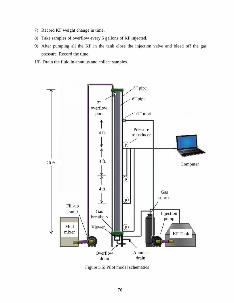
76
7) Record KF weight change in time.
8) Take samples of overflow every 5 gallons of KF injected.
9) After pumping all the KF in the tank close the injection valve and bleed off the gas
pressure. Record the time.
10) Drain the fluid in annulus and collect samples.
Figure 5.5: Pilot model schematics
Computer
6” pipe
Mud
mixer
Pressure
transducer
KF Tank
Overflow
drain
Annular
drain
Injection
pump
Gas
source
Viewer
Fill-up
pump
2”
overflow
port
20 ft.
4 ft.
1/2” inlet
Gas
breathers
P
P
P
P
8” pipe
4 ft.
4 ft.

77
Figure 5.6: Bottom pressure change during experiment
Pressure measurements were obtained automatically from the pressure transducers and also
manually from the pressure gages. The gages specified range of 30 psi and low accuracy and
accuracy of the transducers was ±0.015 psi. However, all the tested transducers except the one at
the bottom had offsets of around 0.1 psi. Nevertheless, only the bottom transducer was used for
the analysis so no corrections were required.
Flowmeter could not be installed on the injection line due to the safety regulations in
Albemarle facility. Therefore, rate was calculated from the mass vs. time measurements.
Therefore, error of the injection rate could only be detected and adjusted for after several minutes
of injection. This method made it difficult to set a desired injection rate, particularly in the first
five minutes of injection. Gas injection rate, on the other hand, could be fixed from a flowmeter
installed on the gas line. After each experimental run, drained fluid samples from the annulus
were tested for concentration of KF and AF. The samples in annulus were drained in different
drums and weighted separately. If a sample density was smaller than density of KF, the sample
was centrifuged to find volume fraction of each component.
5.2.3 Experimental Matrix
Annular fluid (AF) to be used in the pilot scale tests are mixed in a 20 barrel trip tank at
LSU Petroleum Engineering Research & Technology Transfer Laboratory (PERTTL) by using
0
5
10
15
20
0 1 2 3 4
Bott
om
Pre
ssure
, psi
Time, hours
Gel-up duration
Drainage and
sampling
KF injection
Gas
injection AF fill-up

78
different concentrations of bentonite clay and Barite (barium sulfate) to obtain various structural
strengths and densities. Structural strength is defined as a combination of fluid’s resistance to
shear and its gelation capability (rheology and tixotrophy). According to AF’s density and
structural strength level annular fluids are named starting with the letters “AF”. Structural
strength level varies dominantly with the drilling fluid’s clay concentration. As concentration
increases, AF shows higher rheology and higher gel strength. For instance the AF0901 fluid had
9 ppg density and properties the lowest level of structural strength. Annular fluid names,
densities and structural strength are listed in Table 5.1.
When annular fluids with the same density were being mixed, initially the lowest
concentration of bentonite was hydrated in the trip tank overnight. Then, barium sulfate was
added to increase its density to desired value. After taking out some of this low strength
(structural level 1) AF more bentonite is added to increase its structural strength and desired
amount is again taken out after circulating the mud for an hour to attain homogeneity. The same
process was repeated for all AF varieties. The fluids were collected in 30-gallon drums, labeled
and shipped to Albemarle PDC. Samples from each batch of mixing were also collected for
measurement.
Table 5.1: Table of annular fluids (AF) in pilot experiments
Name Density
ppg
Structural
Strength Level
Bentonite concentration
ppb
AF0901 9 1 13
AF0902 9 2 18
AF0903 9 3 25
AF1101 11 1 15
AF1102 11 2 20
AF1103 11 3 25
AF1301 13 1 15
AF1302 13 2 18
AF1303 13 3 22
Each kill fluid (KF) has been produced by blending two of three different components. As
explained in selection kill fluid chapter in this work densities of these components were 11.08,
24.7 and 7.01 ppg and their viscosities were 4090 cP, 2 cP and 13 cP, respectively. Properties of

79
KF used in the pilot tests are listed in Table 4.3. The fluids code represent density and viscosity
degree of the kill fluid. The blends heavier than 15 ppg were produced from the 11.08 ppg and
24.7 ppg components and their viscosities follow the trend shown in Figure 3.3. The KF having
12 ppg density was produced from the 24.7 ppg and 7.01 ppg components and the two blends
(15.1 ppg and 14.91 ppg) were obtained by blending all three components (24.8 ppg, 11.08 ppg,
and 7.01 ppg).
Table 5.2: Properties of annular fluids in pilot experiments
Fluid ρ
(ppg)
μp
(cP)
τ0 (lbf/100sqft)
τg2hours
(lbf/100sqft)
AF0901 9 3.2 2.1 2.1
AF0902 9 10.6 4.2 13
AF0903 9 25.4 14.8 37
AF1101 11 9.5 4.2 5
AF1102 11 21.2 6.4 28
AF1103 11 55 58.3 73
AF1301 13 21.2 9.5 17
AF1302 13 30.8 30.8 32
AF1303 13 38 40.3 75
Table 5.3: Properties of kill fluids used in pilot experiments
Density, ppg Viscosity, cP
Estimated IFT,
dynes/cm
Estimated
log(P)
KF1204 11.8 8.0 32 3
KF1501 15.01 492.0 24 6
KF1502 14.91 12.0 28 3
KF1701 16.68 235.6 21.5 6.5
KF2001 19.6 76.4 29 2
KF2301 22.94 25.5 34 2.5
Table 5.4 shows the AF/KF combinations used in the experiments. Each run are named as
“batch” and number. Batch refers to KF components mixed in the tank. This name has been
selected to avoid confusion with the slot-model experiments. Since supply of brominated organic
material was limited, most of the experiments were run with KF1701. Also, the maximum
injection rate was limited at 6 gpm by the installation.

80
Table 5.4: Experimental matrix of pilot-scale experiments
AF
KF AF0901 AF0902 AF0903 AF1101 AF1102 AF1103 AF1301 AF1302 AF1303
Batch# q, gpm B# q B# q B# q B# q B# q B# q B# q B# q
KF1204
27 1.0
28 6.0
29 4.3
KF1501 20 1.2 21 1.2 11 1.1
KF1502
30 0.8
KF1701
4 1.2 5 1.4 2* 1.1 18 2.2 10 1.1 14 1.3 15 1.2 9 0.9 7 1.0
3* 0.7 31 1.4 16 1.5 19 0.9
6 1.2
KF2001
26 1.0 24 1.0 1* 1.2
12 1.2
33 1.1 8 1.3
35 1.1
32 0.8
22 3.9
23 5.0
KF2301
17 1.3
13 1.1
25 1.3
AF1302
34 1.0
* Concurrent displacement with gas migration

81
Results and Observations
A total of 34 immiscible displacement experiments have been run as shown in Table 5.5. In
all experiments complete displacement was not achieved due limited volume of the kill fluid
(Pressure replacement stopped when there was no more fluid in the KF tank). A few runs, such
as Batch 31, shown in Figure 5.7, with 1.23 annular volumes of KF (Ru=1.23) resulted in almost
complete displacement (Ef=0.97). Typically, as shown in the plot, the bottom pressure buildup
was initially up to a departure point of the curved section that would asymptotically reach the
ultimate pressure value, Pu.
Figure 5.7: Pressure vs. time plot of Batch 31 run; Pmax= maximum final pressure, Pu= ultimate
pressure (complete displacement)
Figure 5.8 demonstrates two examples of unfinished displacement due to KF volume
shortage. The Batch 6 run used only 0.83 annular volumes of KF and did not show any deviation
from linear trend. The Batch 23 run, on the other hand, showed a curvature forming after 1.4
minutes of injection and did reach the complete displacement line despite injecting 1.79 volumes
of KF.
As explained in more details in the experimental procedure, KF injection rates are obtained
without use of a flowmeter. Therefore, as also shown in Figure 5.8 (Batch 6 run), the initial rate
was high before it got under control after minutes of injection. These operational problems
12
13
14
15
16
17
5 10 15 20
Bott
om
Pre
ssu
re,
psi
Time, minutes
q = 1.36 gpmtu = 18.7 minPmax = 16.82 psi
Pu = 16.9 psi
Complete displacement line Pu
Departure point

82
caused multiple flow rates and generated more than one linear trends in the pressure vs time
plots. Averaged flow rates, batch numbers and their corresponding fluid properties are shown in
the results, Table 5.5. In the table, Rf column shows the final displacement ratio when available
volume of KF was injected, and Ef column shows the final pressure replacement efficiencies.
Figure 5.8: Pressure vs. time plots of Batch 6 and Batch 23 runs demonstrate unfinished
displacements due shortage of KF
Fluid samples collected from the overflow and the annulus indicated presence of a mixture
zone on top of the settled clean kill fluid column. This zone had distributed density with depth –
shown in Figure 5.9. Density measurements for minus values of depth are obtained from the
overflow, and positive values are taken from annular drain samples. The general shapes of
density trends are not the same but their curvatures are different.
During an actual bleed-and-lube operation, the pressure bleed-off cycle may induce additional
gas migration. In order to simulate such a scenario (in the Batch 1, 2 and 3 runs) injection of KF
was conducted concurrently with gas injection. Figure 5.10 shows a comparison of the pressure
vs. time plots of the Batch 1 run and Batch 35 run.
The Batch 1 plot shows early curvature indicating loss of KF to overflow resulting from
flotation effect. As the plot’s curvature continues, it indicates an asymptote pressure value below
that for complete displacement. The phenomenon represents an “incomplete displacement” of
annular fluid and is indeed not a desirable performance of the displacement process.
8
9
10
11
12
13
14
15
16
17
0 10 20
Bott
om
Pre
ssure
, psi
Time, minutes
13
14
15
16
17
18
19
20
0 2 4Time, minutes
Batch 6 run
Complete
displacemen
Complete displacement line Complete displacement line
Batch 23 run
Complete
displacemen

83
Figure 5.9: Depth of mixture zone above top of clean KF
Figure 5.10: Comparison plots of pressure buildup with (Batch 1 run) and without concurrent gas
migration (Batch 35 run)
0
2
4
6
8
10
12
14
16
18
20
8 10 12 14 16 18 20 22
Colu
mn h
eight,
ft
Density, ppg
6
8
10
12
14
16
18
20
0 5 10 15 20 25 30
Bott
om
Pre
ssure
, psi
Volume of KF pumped, gal
Stagnant gas-cut AF
Gas migration
Complete displacement line
Column top
Column bottom
Batch 11 run
Batch 8 run
(Batch 35 run)
(Batch 1 run)

84
Table 5.5: Immiscible displacement test results* and analysis
Batch ρkf ppg
μkf cP
ρaf ppg
μaf cP
τ0 lbf/100sqft
τg
lbf/100sqft
q gpm
q gpm
a
ft tL
min tu
min EL Rf Ef Ru
4 16.68 236 8.90 3.18 2.12 2 1.2 1.2 0.85 15.50 17.65 0.92 0.97 0.97 1.04
5 16.68 236 9.00 10.60 4.24 11 1.4 1.4 4.33 13.50 17.79 0.88 0.96 0.92 1.18
6 16.68 236 9.00 25.44 14.84 25 1.2 1.2 1.00 14.00 17.80 0.84 0.84 0.83 1.06
7 16.68 236 12.90 39.22 32.96 71 1.0 1.2 8.36 6.72 23.96 0.51 0.96 0.67 1.41
8 19.60 76 13.01 36.04 31.80 71 1.3 1.3 11.75 7.72 22.78 0.50 0.99 0.88 1.45
9 16.68 236 13.10 28.62 27.56 28 0.9 1.0 3.38 13.72 24.30 0.66 1.02 0.94 1.22
10 16.68 236 10.90 22.79 16.96 25 1.1 1.1 3.28 16.97 23.15 0.83 1.04 0.93 1.21
11 15.60 376 9.11 27.56 27.56 35 1.1 1.1 1 0.00 23.11 1.00 0.98 0.77 1.22
12 19.60 76 11.10 51.94 78.44 69 1.2 1.4 4.13 7.72 18.12 0.52 0.98 0.86 1.26
13 22.94 25 11.00 63.60 74.20 69 1.1 1.2 4.61 11.22 21.40 0.65 0.96 0.95 1.21
14 16.85 219 11.00 60.42 62.54 69 1.3 1.3 8.11 7.48 21.30 0.48 0.99 0.70 1.36
15 16.68 236 13.20 21.20 9.54 16 1.2 1.2 9.31 12.23 22.68 0.73 1.00 0.89 1.36
16 16.68 236 11.00 25.44 20.14 25 1.5 1.5 8.48 12.23 17.72 0.87 1.04 0.89 1.26
17 22.68 28 9.00 29.15 26.50 35 1.3 1.3 4.76 10.73 20.18 0.65 0.87 0.85 1.24
18 16.68 236 10.90 12.72 7.42 5 2.2 2.2 13.93 4.38 13.82 0.50 0.93 0.70 1.46
19 16.68 236 11.00 55.12 69.96 69 0.9 1.0 4.70 19.32 25.69 0.88 1.06 0.97 1.25
20 15.01 492 8.86 6.36 1.06 2 1.2 1.2 1.35 14.32 19.52 0.78 1.01 0.91 1.09
21 15.01 492 8.93 13.78 7.42 12 1.2 1.2 1 0.00 19.43 1.00 1.01 0.93 1.12
22 19.60 76 13.00 36.04 26.50 71 3.9 3.8 11.35 3.98 8.30 0.62 1.04 0.88 1.52
23 19.35 84 13.00 33.92 31.80 71 5.0 5.0 20.09 1.43 7.33 0.35 1.04 0.79 1.79
24 19.60 76 8.90 11.66 8.48 12 1.0 1.0 2.35 17.32 22.17 0.86 1.04 0.92 1.11
25 22.52 29 12.85 39.16 29.68 71 1.3 1.4 5.57 6.65 18.90 0.46 1.04 0.86 1.30
26 19.60 76 8.80 3.18 3.18 2 1.0 1.0 1.21 17.73 21.22 0.88 1.04 0.96 1.08
27 11.80 8 9.10 27.56 20.14 35 1.0 1.0 1.53 19.00 21.02 0.96 0.99 0.95 1.07
28 11.92 8 9.00 28.62 23.32 35 6.0 6.0 11.91 2.82 5.22 0.69 1.04 0.82 1.53
29 11.92 8 9.10 27.56 34.98 35 4.3 4.3 7.45 1.82 6.74 0.34 1.02 0.94 1.41
30 14.91 12 9.00 28.62 29.68 35 0.8 1.0 2.60 16.73 24.01 0.80 1.03 0.92 1.20
31 16.68 236 11.00 11.66 6.36 5 1.4 1.4 4.85 13.73 18.66 0.85 1.29 0.98 1.23
32 19.60 76 11.10 68.90 84.80 69 0.8 1.1 1.80 17.65 22.15 0.88 1.03 0.93 1.15
33 19.60 76 13.00 29.68 37.10 35 1.1 1.1 10.10 10.00 25.02 0.57 1.03 0.90 1.39
35 19.68 74 9.10 28.62 37.10 35 1.1 1.0 6.63 13.32 23.87 0.72 0.90 1.22
*No runs with gas migration (Batch 1, 2, and 3)

85
Analysis of Pilot Testing Results
5.4.1 Process Performance Measures
The main objective of the pilot testing was to test the performance of gravity displacement
process by measuring the hydrostatic pressure change at the bottom of the fluid column. The
ultimate goal of the process is to increase the bottom pressure by displacing the annular fluid; in
a reasonable time. Thus, bottom pressure versus time data from the experiments are used for
calculating the performance measures: pressure replacement efficiency (Ep) and volumetric
efficiency (Ev) or displacement ratio defined as,
Pressure replacement efficiency:
Ep =
∆P
∆Pu=P − PafPu − Paf
(5.1)
Volumetric efficiency:
Ev =
1
R=VaVp
(5.2)
Displacement ratio:
R =
Vp
Va (5.3)
where, ∆P is bottom pressure change, ∆Pu is ultimate bottom pressure difference, P is bottom
pressure, Paf is bottom pressure when the column is filled with only AF, Pu is bottom pressure
when the column is filled with only KF, Va is the volume of annulus (20.5 gal) and Vp is the
volume of KF pumped into the column.
The end of a fully successful ideal displacement process is when the pressure replacement
and volumetric efficiencies are both equal one. Obviously, as already observed from the
experiments, more than one annular volume of kill fluid is required to reach 100% pressure
replacement efficiency. (Therefore, inverse of Ev, volume displacement ratio (R), is used for
computations.) End of the displacement process is defined as the time when the pressure
replacement efficiency is either one, or its value becomes constant and cannot be increased
anymore.

86
5.4.2 Pressure Replacement Model
As most of displacement runs were unfinished due to KF volume shortage, pressure buildup
plots must be extrapolated to determine the end of displacement process. Moreover, the
extrapolation model must have physical sense. Figure 5.11 shows fluid zones in the annulus
during displacement process. During the process, a mixture zone develops above the KF top and
expands. At the time the mixture zone (MZ) reaches the overflow port (t = tL, and zaf = 0), the
overflow density (ρof) starts increasing from the annular fluid density up to the kill fluid density
when the clean KF comes to the top (zkf = 0). The moment when KF column reaches the
overflow port indicates the ultimate time of displacement (tu).
Figure 5.11: Fluid zones distribution in annulus: kill fluid (KF), mixture zone (MZ) and annular
fluid (AF)
In most of the experiments displacement stopped when the mixture zone was already
overflowing. In order to extrapolate the process duration mixture zone density must be related to
density change in overflow. Exponential distribution of mixture zone density, shown in Figure
5.9, has been fitted with exponential function and the plots in Figure 5.12 demonstrate good
match.
MZ

87
Figure 5.12: Exponential fit of mixture zone density with exponent (6) shows good match
Thus, density distribution in the annulus at any time,
ρa(z) = ρaf for 0 < z < zaf (5.4)
ρa(z) = ρaf + (ρkf − ρaf) exp (−zkf − z
a) for zaf < z < zkf (5.5)
ρa(z) = ρkf for zkf < z (5.6)
where, z = depth below top of annulus
zaf = depth of AF section
zkf = depth of clean KF section top
Since, function 5.5; asymptotically approaches annular fluid density,
limz→∞
ρaf + (ρkf − ρaf) exp (−zkf − z
a) ≅ρaf
depth of AF section, zaf, is defined by setting small value, TOL, as TOL = [ρa(zaf) − ρaf] ≪ 1.
In general, length of the mixture zone, increases with time but the overflow density, ρof, remains
constant (ρof = ρaf) until the top of mixture zone comes to the overflow port so,
for 0 < t < tL ρof = ρaf (5.7)
where: tL= end of linear trend
9
11
13
15
17
19
0 5 10 15 20 25
Den
sity
, ppg
Height above KF top, ft
Batch 8 run
Batch 11 run

88
Later, no change in the mixture zone composition is assumed. With this assumption, travel
distance of each point in the mixture zone becomes linear function of time,
z(t) = −q
At
Where, q is injection rate and A is annular capacity.
As the mixture zone passes the overflow port, its length decreases at linear velocity, dz dt⁄ =
−q A⁄ and, concurrently the overflow density increases from ρaf to ρkf. The ultimate time, tu, is
when the clean kill fluid top reaches the overflow port, and zkf = 0.
Thus, the overflow density change vs. time (Equation 5.5) is,
ρof(t) = ρaf + (ρkf − ρaf) exp (−q
A
(tu − t)
a) for 0 < t < tL (5.8)
Overflow density change during the Batch 12 displacement run is shown in Figure 5.13.
Before and after mixture zone is displaced, annular fluid and kill fluid start flowing out. This
brings two discontinuity points: the time when clean annular fluid finishes and mixture zone
starts overflowing (tL), and the time when mixture zone finishes and clean kill fluid starts
overflowing (tu). Figure 5.13 shows these points and fit functions on measured overflowing
density data.
Figure 5.13: Overflowing density change during Batch12 experimental data
9
11
13
15
17
19
0 5 10 15 20 25 30
Over
flow
den
sity
, ppg
Time, min
OF density = AF density = constant = 11 ppg
OF density = AF density = constant = 19.6 ppg
Equation (5.8) (a=5)
Measured
tL tu

89
As shown in Appendix B, overflow density change is mathematically related to the change of
fluid mass in the annular column using two assumptions: (1) Constant-rate injection of KF; and
(2) Constant composition of mixture zone during the zone discharge.
During displacement of clean annular fluid, the annulus mass is,
ma(t) = maf + q (ρkf − ρaf ) t (5.9)
During charge of mixture zone, the annular mass is,
ma(t) = maf + q (ρkf − ρaf) t
− aA(ρkf − ρaf) exp (−q
Aatu) [ exp (
q
Aat) − 1]
(5.10)
At the end of mixture zone discharge, the annular mass is constant and equal to the mass of
kill fluid, mkf. Where, maf and mkf represent annular fluid mass full of annular and kill fluids,
respectively.
After converting fluid mass to hydrostatic bottom pressure, mathematical model of the
pressure replacement process is developed as follows.
For displacement of annular fluid stage,
Pba(t) = Paf + 0.052q
A ∆ρ t for
0 ≤ t ≤ tL
(5.11)
0 ≤ P ≤ PL
For change of mixture zone stage,
Pba(t) = PL +0.052 q ∆ρ
A(t − tL)
− 0.052 a ∆ρ exp (−q
Aa(tu − tL)) [ exp (
q
Aa(t − tL)) − 1]
(5.12)
for tL ≤ t < tu and PL ≤ P < Pe.
After the mixture zone discharge, ultimate pressure, Pu, is reached: 𝑃𝑢 = 0.052 𝜌𝑘𝑓 𝑉𝑎 𝐴⁄

90
Note, that Equation 5.12 for t=tu relates (typically unknown) mixture zone parameter “a” to
the measured values of tL and tu, as,
Pu = PL + 0.052∆ρ [ q
A(tu − tL) − a + a exp (−
q
Aa(tu − tL))]
(5.13)
In dimensionless formulation, using the process performance measures, Ep and R – defined
above, the pressure replacement model (Appendix B) becomes as follows.
For displacement of annular fluid (linear pressure increase), 0 ≤ R ≤ RL and 0 ≤ Ep ≤ EpL;
Ep(R) = R =Vp
Va=
qt
haA
For mixture zone discharge stage, RL ≤ R ≤ Ru or EpL ≤ Ep ≤ 1;
Ep(R) = R −
a
ha exp (−
haa(Ru − RL)) [ exp (
haa(R − RL)) − 1] (5.14)
After the mixture zone discharge (R ≥ Ru),
Ep(R) = 1
Note that for ultimate displacement ratio, Equation 5.14 equals unity and relates the
(typically) unknown mixture zone parameter “a” to the measured values of RL and Ru from the
tests, as,
E(Ru) = 1 = Ru −a
ha exp (−
haa(Ru − RL)) [ exp(
haa(Ru − RL)) − 1]
Solving for RL gives,
RL =a
haln (1 −
haa(Ru − 1)) + Ru (5.15)
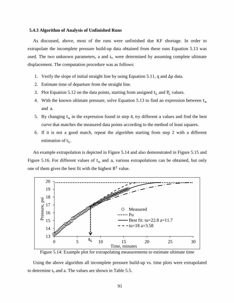
91
5.4.3 Algorithm of Analysis of Unfinished Runs
As discussed, above, most of the runs were unfinished due KF shortage. In order to
extrapolate the incomplete pressure build-up data obtained from these runs Equation 5.13 was
used. The two unknown parameters, a and tu, were determined by assuming complete ultimate
displacement. The computation procedure was as follows:
1. Verify the slope of initial straight line by using Equation 5.11, q and ∆ρ data.
2. Estimate time of departure from the straight line.
3. Plot Equation 5.12 on the data points, starting from assigned tL and PL values.
4. With the known ultimate pressure, solve Equation 5.13 to find an expression between tu
and a.
5. By changing tu in the expression found in step 4, try different a values and find the best
curve that matches the measured data points according to the method of least squares.
6. If it is not a good match, repeat the algorithm starting from step 2 with a different
estimation of tL.
An example extrapolation is depicted in Figure 5.14 and also demonstrated in Figure 5.15 and
Figure 5.16. For different values of tu and a, various extrapolations can be obtained, but only
one of them gives the best fit with the highest R2 value.
Figure 5.14: Example plot for extrapolating measurements to estimate ultimate time
Using the above algorithm all incomplete pressure build-up vs. time plots were extrapolated
to determine tu and a. The values are shown in Table 5.5.
13
14
15
16
17
18
19
20
0 5 10 15 20 25 30
Pre
ssure
, psi
Time, minutes
Measured
Pu
Best fit: tu=22.8 a=11.7
tu=18 a=3.58
𝐭𝐋

92
Figure 5.15: Extrapolation of pressure buildup for Batch 10 run
Empirical Correlations
5.5.1 Trend Analysis
Figure 5.17 shows the change in performance parameters with increasing density of annular
fluid, and consequently due to structural strength h, occurred as a result of higher barite
concentrations. For all three runs flow rate was around the same value and the volumes of
injected kill fluid were similar. According to the plot, as the density of annular fluid increases,
departure from linear pressure build-up occurs earlier. Therefore, mixture zone overflow starts
much sooner for heavier annular fluids, as also can be understood from the increase in
exponential coefficient. Accordingly, maximum obtainable efficiency for one annular volume
injection reduces significantly as the density goes up.
Figure 5.16: Extrapolation of pressure buildup for Batch 12 run
10
12
14
16
0 5 10 15 20 25
Bott
om
Pre
ssure
, psi
Time, minutes
MeasuredExtrapolationPutu
11
13
15
17
19
0 5 10 15 20
Bott
om
pre
ssure
, psi
Time, minutes
MeasuredExtrapolationPutu
mt = m = 0.53q = 1.4 gpmq = 1.7 gpmtu = 18.1 minRu = 1.26
mt = m = 0.31
q = 1.07 gpm
tu = 23.1 min
Ru = 1.21

93
Figure 5.17: Change in dimensionless values and exponential coefficient with increasing annular
fluid density. Batches 4, 31 and 15 runs show the effectiveness of the process when lighter and
low structural strength AF is present
Shown in Figure 5.18 are the trends of performance change with increasing injection rate. The
most obvious result of faster injection is the ultimate displacement ratio, which increases to ~1.5
with increasing flow rate. In other words, about 1.5 times more kill fluid provides a complete
displacement when injecting with 6 gpm than injecting with 1 gpm. The process inefficiency
increase results from the change of mixture zone coefficient “a” that determines the mixture zone
size. It should also be noted that pressure replacement efficiency, Ep, was equal unity in all
experiments for the range of injection rates applied.
Figure 5.18: Change in dimensionless values and exponential coefficient with increasing flow
rate. KF1204 injections into AF0903 with different rates (Batches 27, 28 and 29) show
increasing mixture zone height and more losses to overflow with increasing rate
0
2
4
6
8
10
0.7
0.8
0.9
1
1.1
1.2
1.3
1.4
8 9 10 11 12 13 14
a, f
eet
Dim
ensi
onle
ss v
alue
Annular Fluid Density, ppg
Ru
RL
a
0
2
4
6
8
10
12
14
0
0.2
0.4
0.6
0.8
1
1.2
1.4
1.6
1.8
0.0 1.0 2.0 3.0 4.0 5.0 6.0 7.0
a, f
eet
Dim
ensi
onle
ss v
alue
Flow rate, gpm
Ru
a
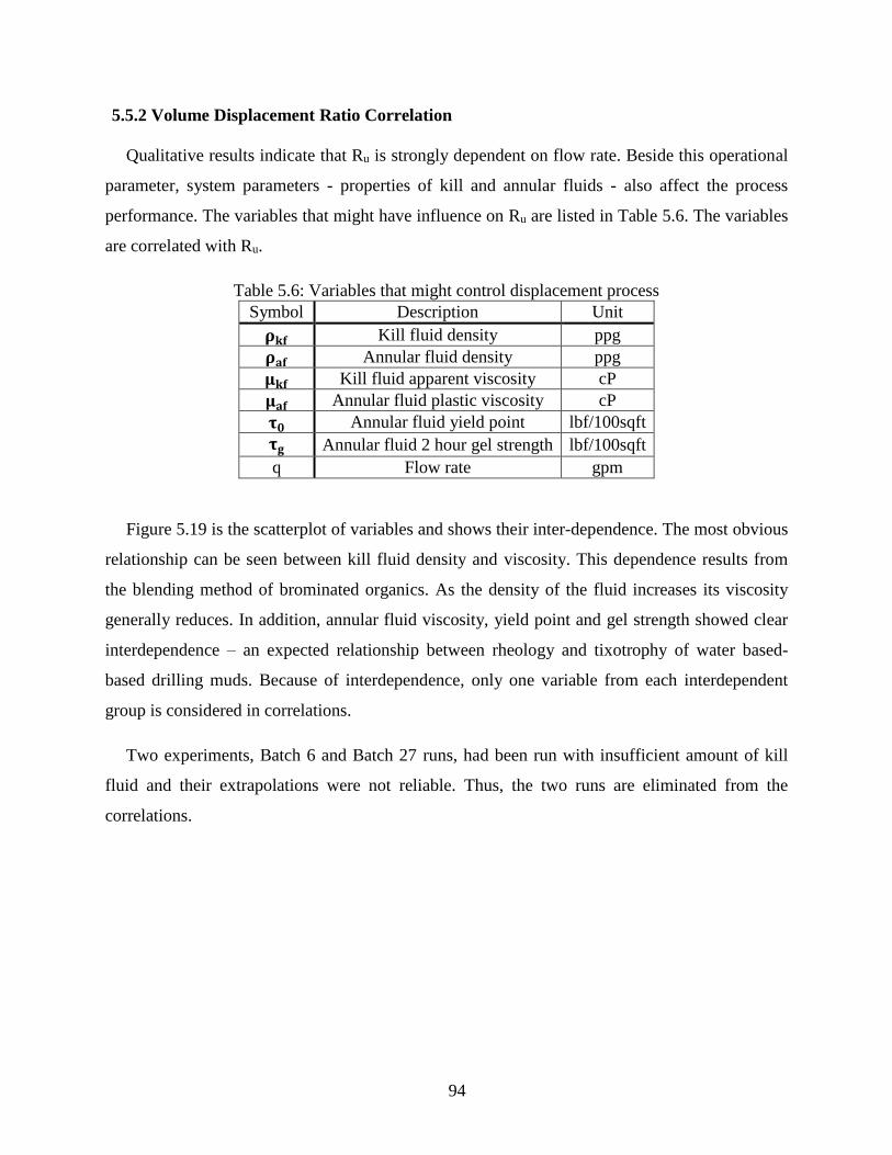
94
5.5.2 Volume Displacement Ratio Correlation
Qualitative results indicate that Ru is strongly dependent on flow rate. Beside this operational
parameter, system parameters - properties of kill and annular fluids - also affect the process
performance. The variables that might have influence on Ru are listed in Table 5.6. The variables
are correlated with Ru.
Table 5.6: Variables that might control displacement process
Symbol Description Unit
𝛒𝐤𝐟 Kill fluid density ppg
𝛒𝐚𝐟 Annular fluid density ppg
𝛍𝐤𝐟 Kill fluid apparent viscosity cP
𝛍𝐚𝐟 Annular fluid plastic viscosity cP
𝛕𝟎 Annular fluid yield point lbf/100sqft
𝛕𝐠 Annular fluid 2 hour gel strength lbf/100sqft
q Flow rate gpm
Figure 5.19 is the scatterplot of variables and shows their inter-dependence. The most obvious
relationship can be seen between kill fluid density and viscosity. This dependence results from
the blending method of brominated organics. As the density of the fluid increases its viscosity
generally reduces. In addition, annular fluid viscosity, yield point and gel strength showed clear
interdependence – an expected relationship between rheology and tixotrophy of water based-
based drilling muds. Because of interdependence, only one variable from each interdependent
group is considered in correlations.
Two experiments, Batch 6 and Batch 27 runs, had been run with insufficient amount of kill
fluid and their extrapolations were not reliable. Thus, the two runs are eliminated from the
correlations.

95
Figure 5.19: Scatter plot of experimental variables
By using all the variables that may affect the displacement process (variables in Table 5.6) a
prediction expression with a coefficient of determination (R2) of 0.896 is first obtained.
Parameter estimates is shown under initial prediction column in Table 5.7 and leverage plots are
drawn in Figure 5.20. In the initial prediction despite the high R2 value, t-Ratio values – which
represent the ratio of estimate over estimate standard error – of several parameters are found as
quite low. A significant variable generally should have an absolute t-ratio value greater than 2.
Leverage plots in Figure 5.20 also show the insignificance of several parameters. Leverage plots
are used for seeing which points might be exerting influence on the hypothesis test for the
variable. In other words, a leverage plot for an effect shows the impact of adding this effect to
the model, given the other effects already in the predictive model. In the plots, distance between
the points to fit line (red) gives the error when the variable is in the predicted model; and the
distance between the point and horizontal line (blue) gives the error when the variable is
removed from the model. The cloud-like plots confirm the annular fluid properties
interdependence, which causes a collinearity problem so that only one variable should be
considered in the correlation.

96
Figure 5.20: Leverage plots of Ru residuals vs. all the variables
Table 5.7: Summary and parameter estimates of the fits
Initial Prediction Final Prediction
R2 0.896 0.878
R2 adj 0.86 0.857
Root Mean Square Error 0.020 0.021
Mean of Response 0.104 0.104
Data Count 29 29
Term Estimate Std.
Error t Ratio Estimate
Std.
Error t Ratio
Intercept -0.3781 0.0826 -4.58 -0.3759 0.0794 -4.74
log10 ρaf 0.3062 0.0790 3.87 0.3771 0.0685 5.51
log10 μkf 0.0181 0.01 1.81 - - -
log10 τ0 0.0164 0.0278 0.59 0.0187 0.00904 2.07
log10 q 0.1882 0.0208 9.04 0.1719 0.01832 9.38
log10 ρkf 0.0485 0.0614 0.79 0.0351 0.0597 0.59
log10 τg 0.0074 0.0292 0.25 - - -
log10 μaf 0.0091 0.0465 0.19 - - -

97
By eliminating the insignificant parameters one by one, the best expression for Ru is obtained
by using only annular fluid density, and yield point, kill fluid viscosity (or density) and injection
rate. Statistical analysis is shown in Table 5.7 - final prediction column. Figure 5.21 shows the
prediction plot and Equation 5.16 is the predicted expression and gives an R2 value of 0.878.
Excluded points are also shown in the prediction plot with the cross shapes. In the figure, the red
solid line is the 45° line and represents the goodness of the fit. The red dashed lines give the 95%
confidence interval and blue dashed line is the mean value of actual displacement ratios.
Predicted Expression for displacement ratio:
Ru = 10−0.376 ρaf
0.377 ρkf0.035 τ0
0.019 q0.1719 (5.16)
Figure 5.22 shows the prediction profiler of variables. In this figure, X-axis shows the
variables, and the red numbers indicates their current values. Y-axis gives the corresponding Ru
value and red numbers show the corresponding Ru for the current values of the variables. Black
lines give the changing Ru when that particular variable is being changed while the others remain
constant. Based on the figure and Equation 5.16, the most significant variable is flow rate, and
second dominant variable is annular fluid density. Kill fluid density and annular fluid yield point
have some effect on Ru but not significant.
Figure 5.21: logRu actual versus logRu predicted with corrleation in Equation 5.16 (Properties are
shown in Table 5.7
(logR
u)
Mea
sure
d
(logRu) Predicted Ru, R2=0.88
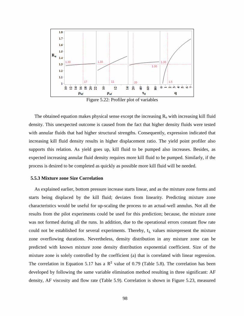
98
Figure 5.22: Profiler plot of variables
The obtained equation makes physical sense except the increasing Ru with increasing kill fluid
density. This unexpected outcome is caused from the fact that higher density fluids were tested
with annular fluids that had higher structural strengths. Consequently, expression indicated that
increasing kill fluid density results in higher displacement ratio. The yield point profiler also
supports this relation. As yield goes up, kill fluid to be pumped also increases. Besides, as
expected increasing annular fluid density requires more kill fluid to be pumped. Similarly, if the
process is desired to be completed as quickly as possible more kill fluid will be needed.
5.5.3 Mixture zone Size Correlation
As explained earlier, bottom pressure increase starts linear, and as the mixture zone forms and
starts being displaced by the kill fluid; deviates from linearity. Predicting mixture zone
characteristics would be useful for up-scaling the process to an actual-well annulus. Not all the
results from the pilot experiments could be used for this prediction; because, the mixture zone
was not formed during all the runs. In addition, due to the operational errors constant flow rate
could not be established for several experiments. Thereby, tL values misrepresent the mixture
zone overflowing durations. Nevertheless, density distribution in any mixture zone can be
predicted with known mixture zone density distribution exponential coefficient. Size of the
mixture zone is solely controlled by the coefficient (a) that is correlated with linear regression.
The correlation in Equation 5.17 has a R2 value of 0.79 (Table 5.8). The correlation has been
developed by following the same variable elimination method resulting in three significant: AF
density, AF viscosity and flow rate (Table 5.9). Correlation is shown in Figure 5.23, measured

99
data is scattered through around the prediction line; therefore, using experimental data – when
available – instead of the correlation is recommended.
Table 5.8: Summary of fit for predicting exponential coefficient
R2 0.79
R2 adjusted 0.76
Root Mean Square Error 0.16
Mean of Response 0.704
Data Count 25
Table 5.9: Parameter estimates calculated for predicting exponential coefficient
Term Estimate Std.
Error
t
Ratio
Intercept -1.606 0.5123 -3.13
log10 ρaf 1.5525 0.5600 2.77
log10 q 0.6619 0.1394 4.75
log10 μaf 0.4461 0.1122 3.98
Figure 5.23: Prediction plot of mixture zone exponential coefficient
a = 10−1.61 ρaf1.55 μaf
0.45 q0.66 (5.17)
(log a
) M
easu
red
(log a) Predicted Ru, R2=0.79

100
The plot in Figure 5.24 shows the change in exponential coefficient with increasing flow rate
and annular fluid viscosity. As can be seen, faster injection rates and higher viscosities result in
greater coefficients, which indicate a larger mixture zone.
Figure 5.24: Mixture zone coefficient vs. flow rate for different AF viscosities for AF density 12
ppg
5.5.4 Use of Correlations for Design
Using the empirical model, described above, for predicting performance of the displacement
process in 20-foot pilot to the field-length annulus. The upscaling is limited by the following
assumptions:
1. Well-head pressure stays constant during the displacement process so there is no new gas
entry to the fluid column.
2. Injection rate is constant.
3. Injection rate does not exceed its maximum value.
4. Scaling factor for the process performance is the ratio of fluid column length in the pilot
model and the well annulus.
The third assumption implies a designed rate of kill fluid that would not cause initial
dispersion (qcr−i) as described in chapter 4.4 and would not exceed the rate of buoyant settling
(qcr−T) defined in the following chapter.
0
5
10
15
20
25
0 2 4 6 8 10
MZ
coef
fiei
cnt,
a, fe
et
Flow rate, gpm
1 cP

101
The fourth assumption entails hydraulic similarity of steady-state counter-current buoyant
slippage in the pilot model and a full-scale annulus. The assumption awaits further experimental
verification.
Under the light of the learnings from the experiments, process design models can be
employed for any up-scaling attempt.
For a designed injection rate necessary volume of kill fluid to be used in displacement
operation can be found from Equation 5.45 (remembering: Ru = Vpumped/Vannulus).
Ru = 10−0.376 ρaf0.377 ρkf
0.035 τ00.019 q0.1719 (5.16)
A similar modification gives the time needed for complete displacement.
Considering the Ru definition,
Ru =1
Ev=Vp
Va=qtuVa
time needed for complete displacement is,
Pressure replacement efficiency can be estimated by using the fourth assumption to define
scaling factor, k, as,
k =hannulushpilot
Thus, dimensionless pressure replacement versus displacement ratio equations (Equation
5.14) can be rewritten as,
For, 0 ≤ R ≤ RL Ep(R) = R
and for, RL ≤ R ≤ Ru (or EpL ≤ Ep ≤ 1)
tu [hours] = 7.01 ∗ 10−3 ρaf0.377 ρkf
0.035 τ00.019 q−0.8281 Va (5.18)

102
Ep(R) = R −
ka
ha exp (−
haka(Ru − RL)) [ exp (
haka(R − RL)) − 1] (5.19)
Since for R ≥ Ru Ep(R) ≡ 1
it is possible to back calculate RL as,
RL = Ru +k a
haln (1 −
hak a
(Ru − 1)) (5.20)
After estimating the values of “Ru” and “a” from the correlations,the above equations can be
used for predicting a dimensionless plot for any length of well annulus. An example upscaling
design is presented by using the values in Table 5.10. Dimensionless trends are plotted by using
the critical injection rates and shown in Figure 5.25.
Table 5.10: Parameters used for upscaling example
Outer casing size, in 9-5/8” (9.001” ID) AF density, ppg 9
Inner casing size, in 7” (7” OD) AF viscosity, cP 10
Annular capacity, gal/ft 1.31 Yield point, lbf/100sqft 2
Annulus height, ft 4000 KF density, ppg 17
Annular volume, gal 5225 KF viscosity, cP 20
k 205.3 Interfacial tension, dynes/cm 22
qcr−i, gpm 1.1 qcr−A, gpm 2.5
qcr−T, gpm 10.7
To learn the bottom pressure at any particular moment; time can be converted into
displacement ratio. Then, pressure replacement efficiency can be either read from the plot or
calculated from the equations and converted to bottom pressure value. The example plot is
shown in Figure 5.26. The example demonstrates the effect of injection rate that may not always
be designed at maximum. At high rates, more KF is needed but the operation time is shorter.
Thus, the KF cost should be balanced with the well-site hourly cost.

103
Figure 5.25: Example upscaled dimensionless displacement process at various flow rates.
Increasing rate results in early deviation from 45 degree line.
Figure 5.26: Duration of displacement of three different critical rates for upscaling example
Maximum Injection Rate for Buoyant Settling
Results of the slot and pilot model experiments have shown that excessive KF injection rate
reduces efficiency of displacement by: (1) causing KF dispersion at the injection port, and (2)
increasing the counter-current flow rate and the KF reversal effect. The latter effect requires
finding a maximum value of KF injection rate for efficient buoyant transport of this fluid
downwards.
0
0.2
0.4
0.6
0.8
1
0 0.2 0.4 0.6 0.8 1 1.2 1.4 1.6 1.8
E
R
q=1.1 gpm
q=2.51 gpm
q=10.7 gpm
0
0.2
0.4
0.6
0.8
1
0 20 40 60 80 100
E
Duration of displacement, hours
q= 1.1 gpm
q= 2.51 gpm
q= 10.7 gpm

104
The efficient buoyant transport occurs when the system is fed with kill fluid (KF) not faster
than the previously-injected KF travels downwards. Assuming that KF does not form a rope but
breaks-up into droplets, transport rate of the KF can be predicted using the droplet slip velocity
theory. Transport velocity (ϑT) of a concentrated fluid column is slower than the velocity of a
single droplet (ϑd) thus can be represented as multiplication of droplet velocity by a correction
factor, ∈ ≤ 1, as,
ϑT = ∈ ϑd (5.21)
Dedegil [26] developed an equation that represents the velocity of a solid particle in non-
Newtonian media.
ϑp = √2
CDρf(2
3(ρ − ρf) d g − πτ0)
that to be used for droplet velocity, in field units is,
ϑd = √0.27
CDρaf(13.23 ∆ρ d − τ0) (5.22)
Where, ϑd is velocity of a single droplet in ft/sec, CD is drag coefficient acting on slipping
droplet, ρaf is annular fluid density in ppg, ∆ρ is density differential between droplet and
stagnant fluid in ppg, τ0 is yield stress of stagnant fluid in lbf/100sqft and d is equivalent droplet
diameter in inches.
Bozzano and Dente [31] developed drag coefficient equations for liquid droplets at terminal
velocities dependent upon values of the asymptotic friction function (𝑓∞) as follows:
𝑓∞ = 0.9
Eo12
1.4 (1 + 30Mo16) + Eo
32
(5.23)
For f∞ < 0.45,
CD =
48
Re √1 + 0.25 Re
1 + √1 + 0.25 Re
3 2⁄ + μaf μkf⁄
1 + μaf μkf⁄ 1 + 12 Mo
13
1 + 36 Mo13
+ 0.45 (5.24)

105
For f∞ ≥ 0.45,
CD =48
Re √1 + 0.25 Re
1 + √1 + 0.25 Re
3 2⁄ + μaf μkf⁄
1 + μaf μkf⁄ 1 + 12 Mo
13
1 + 36 Mo13
+ 0.9 Eo
12
1.4 (1 + 30Mo16) + Eo
32
(5.25)
Where, dimensionless Morton (Mo) Number and Eötvös Number (Eo) are,
Mo =∆ρ g μaf
4
ρaf2 σ3
Eo = ∆ρ g d2
σ
or in field units,
Mo = 8.2 10−5∆ρ μaf
4
ρaf2 σ3
Eo = 23.6 ∆ρd2
σ
and particle Reynolds number to calculate drag coefficient is,
Re = 928
ρafϑpd
μaf
There are several studies addressing the effect of geometrical restriction on terminal velocity
of particles (Richardson and Zaki [72], Di Felice [73], Kaneda [74], Koch and Sangani [75], Koch and
Hill [76], all qtd. in Multiphase Flow Handbook [13]). Wen and Wu [77] presented a correction for
the effect of particle concentration in a contained system as,
CD = CD0(1 − C)−3.7 (5.26)
where, CD0 is drag coefficient of a single particle and C is particles’ concentration in the system.
Wen and Wu [77] included the effects of relative Reynolds number in the expression for the
terminal velocity of a single particle. Thus, their correlation for the effect of concentration
became independent of the Reynolds number and, therefore, is represented with the constant

106
value, -3.7. The correlation is widely used in fluidization systems [13] and also practical for
computer coding, so, it is selected for this study.
All the above equations include size (diameter) of fluid droplets. For eliminating the droplet
diameter (d), maximum stable diameter of a droplet traveling in a stagnant media developed by
Clift and Weber [30] can be used. Maximum stable droplet diameter in field units is,
dmax ≈ 0.14 (σ ∆ρ⁄ )1 2⁄ (5.27)
Substituting dmax and particle velocity to Reynolds number gives,
Re = 130ρafϑ𝑝
μaf√σ
∆ρ (5.28)
Eötvös number for maximum droplet size becomes constant as,
Eo = 23.6 ∆ρ
σ (0.14 (
σ
∆ρ)1 2⁄
)
2
= 0.46
Also, substituting maximum stable droplet diameter and including concentration correction
into particle velocity formula (Equation 5.22) gives the transport velocity as,
ϑT = √0.27
CDρaf(1.85 √σ ∆ρ − τ0) (5.29)
Above equation assumes that the maximum stable droplet diameter will be achieved and
maintained as the kill fluid stream travels downwards. By substituting Equation 5.29 (after
writing corrected drag coefficient in place, CD = CD0(1 − C)−3.7) and Equation 5.22 we can
define the correction factor as,
∈ = √3.7(1 − C)3.71.85 √σ ∆ρ − τ013.23 ∆ρ d − τ0
In steady-state transport, concentration can be defined using material balance of KF in a unit-
length volume of annulus. For constant feed rate into the unit volume, if the transport velocity is

107
too slow, KF concentration would increase. On the other hand, when velocity is high,
concentration may become negligibly small. Thus, concentration of KF in the annular fluid
column is,
C =q
60 A ϑT (5.30)
The formula relates flow rate (injection rate) to transport velocity and kill fluid concentration
as,
qc = 60 A ϑT C (5.31)
Equation 5.31 implies that, for a given injection rate, qc, when transport velocity is small,
concentration becomes high that, in turn (considering Equation 5.29), further reduces transport
velocity causing chain-reaction that would stop the displacement process. By substituting
Equation 5.29 and to 5.31 equilibrium injection rate can be defined resulting in KF
concentration, C, as,
qc = 31.18 A C√(1 − C)3.7
CD0ρaf(1.85 √σ ∆ρ − τ0) (5.32)
Equation 5.32 directly relates injection rate with fluid concentration. In order to determine
relationship between injection rate and transport velocity the following trial-and-error procedure
is used.
1. Guess an initial value of ϑT.
2. Calculate asymptotic friction factor from Equation 5.23.
3. Calculate Reynolds Number from Equation 5.28.
4. Calculate uncorrected drag coefficient from Equation 5.24 or 5.25.
5. Find concentration from Equation 5.30.
6. Correct drag coefficient for concentration from Equation 5.26.
7. Find new transport velocity from Equation 5.29.
8. Repeat steps 1 through 6 until matching the two values of transport velocity.
9. Find the corresponding flow rate from Equation 5.31.
The above algorithm has been coded in Matlab as shown in Appendix D. Results from
example calculations are plotted in Figure 5.27. The top-left plot in Figure 5.27 depicts the effect

108
of concentration on transport velocity. For the lowest concentration, maximum transport velocity
can be reached. When concentration is too high, transportation velocity approaches zero value.
Interestingly, the plots of injection rate vs. concentration (top right) and vs. transport velocity
(bottom left) have maximum. The maximum value represents the only combination of the rate,
velocity and concentration that makes the rate of KF settling equal to injection rate- the condition
for steady-state settling. Thus, the maximum flow rate is the desired critical flow rate (qcr−T) and
is analytically calculated below.
First derivative of corresponding flow rate formula is,
dqcdC
=d
dC[60AC√
0.27 (1 − C)3.7
CD0ρaf(1.85 √σ ∆ρ − τ0) ] (5.33)
After defining constant, G, as,
G = √
0.27
CD0ρaf(1.85 √σ ∆ρ − τ0) (5.34)
and differentiation, equation for maximum qc can be written as,
dqcdC
= 60 AG [√(1 − C)3.7 +−3.7 (1 − C)2.7
2 √(1 − C)3.7 C] = 0 (5.35)
having only one root,
C = 0.35
Substituting the C=0.35 value into Equation 5.32 gives a closed formula for injection rate,
qcr−T = qc(C = 0.35) = 4.92 A √
(1.85 √σ ∆ρ − τ0)
CD0ρaf (5.36)
It must be emphasized, here, that validity of the critical rate formula (Equation 5.46) is limited
by validity of two empirical correlations: (1) maximum stable droplet size, Equation 5.27, and
(2) corrected drag coefficient, Equation 5.26. Nevertheless, the formula gives useful estimation
for designing the displacement process.

109
Figure 5.27: KF injection rate design plots (τ0 = 2 lbf 100sqft⁄ , ρaf = 8.6 ppg, μkf = 8 cP, μaf = 5 cP, σ = 30 dyne/cm and A =0.24 gal/ft)
KF concentration, fraction
KF
inje
ctio
n r
ate,
gpm
K
F i
nje
ctio
n r
ate,
gpm
Transport velocity, ft/sec
KF concentration, fraction Transport velocity, ft/sec
KF
inje
ctio
n r
ate,
gp
m
Tra
nsp
ort
vel
oci
ty,
ft/s
ec
KF concentration, fraction
𝜌𝑘𝑓 = 12
𝜌𝑘𝑓 = 20
𝜌𝑘𝑓 = 12
𝜌𝑘𝑓 = 12
𝜌𝑘𝑓 = 12
𝜌𝑘𝑓 = 20
𝜌𝑘𝑓 = 20
𝜌𝑘𝑓 = 20

110
CHAPTER 6: FULL SCALE TEST
As demonstrated in pilot-scale testing, above; brominated organics would completely displace
Non-Newtonian fluids and increase the bottom pressure. However, effectiveness of the
displacement process remains unknown for fluid column longer than 20-foot. Moreover, the
process performance may be also affected by surface pressure at the casing head. A single
full0size test was conducted with the following objectives:
Investigate efficiency of the displacement process under surface pressure (SCP);
verify performance of displacement in long fluid column; and,
test validity of the up-scaling model.
Methodology
6.1.1 Well installation
For the test, Well #1 in the LSU Petroleum Engineering Research & Technology Transfer
Laboratory was designated. Schematics of the well can be seen in Figure 6.1. A 2-7/8”
(ID=2.441”) tubing was installed in 5-1/2” and 10-3/4” intermediate casings. The tubing was
2750’ and had 16 barrels volumetric capacity (0.24 gal/ft.). A gas injection valve was installed at
2717’ depth, and two pressure transducers were attached to 1650’ and 2728’ feet depths. A check
valve that allowed one-way flow from annulus into tubing was connected to the bottom of the
tubing. Considering the kill fluid removal problem from the 2-7/8” - 5-1/2” annulus, the
displacement would take place in the 2-7/8” tubing. For top-injection of fluid injection a 0.5”
(ID=0.375”) diameter 60-ft long micro-tubing with an elbow on its end was installed at the
wellhead. Well #4 was used as a source of natural gas to transfer pressure into the annulus. A 2”
flow-line was also attached to the wellhead to receive the overflowing fluid. A conductivity-
meter on the flow-line would measure composition of the overflow stream. A pressure-
temperature transducer at the flow-line was connected to an auto-choke to regulate the pressure.
The flow-line discharged to a mud-gas separator. In addition, a sampling port was assembled
between the transducers and the wellhead to be able to obtain samples and visually inspect the
overflowing fluid. Injection would be provided by a positive displacement chemical resistant
pump that was able to reach up to 900 psi and 9-90 gallons per hour. Steel high-pressure tubing
was connected to the wellhead from the pump and a totalizer/flow meter was installed to be able

111
to read the flow rate and the volume of fluid injected for each batch. Schematics of the full-scale
installation can be seen in Figure 6.2 and a picture of the surface well installation is shown in
Figure 6.3.
Figure 6.1: Well#1 schematics
A 11.85 ppg low-viscosity (8 cP) kill fluid was used to enable efficient cleaning after the test.
The displaced (annular) fluid (AF) was slightly weighted bentonite drilling mud having 8.6 ppg
density. Properties of both fluids can be seen in Table 6.1. A total of 32 barrels of kill fluid was
blended at the facility using three of 550 gallons capacity totes. A 20-barrel trip tank was usd to
prepare the annular fluid. The mixed mud was stored and hydrated in the tank for a week.
5-1/2” Gas injection line (Well #4)
Inflow line
10-3/4” Casing (2788’)
Gas Lift Valve @ 2717’
Gauge Mandrel –
Check valve
attached to the
tubing @2750’
2-7/8” Flow line
2-7/8” Tubing – 16 bbl (2788’)
5-1/2” Casing (2724’)
Pressure-
Temperature
Transducer
@ 2728’
Pressure-
Temperature
Transducer
@ 1650’

112
Table 6.1: Properties of the kill and annular fluids
Kill Fluid Annular Fluid
Type Brominated Organic Blend Water-Based Mud
Density, ppg 11.85 8.6
Viscosity, cP 8 5
Yield Point , lbf/100sqft - 2
Figure 6.2: Full-scale test – well installation
2750 f
eet
T
P F
P
S C
G
PT
PT
Elements shown in the figure:
S: Mud-Gas Separator
A: Auto-choke
PT: Pressure and Temperature
transducers
C: Sampling port
F: Flow meter / Totalizer
P: Fluid injection pump
T: Totes
G: Gas injection valve
2717 f
eet
1590’
1078’
60’
22’
T
A
27
28
fee
t
1650 f
eet

113
Figure 6.3: Picture of well installation
6.1.2 Testing Procedure
1) Fill the tubing 15.5 barrels of the mud by leaving 57 feet space at the top in order to
create a gas cap and to obtain submerged kill fluid injection
2) Close all the valves; trap the mud in the tubing and keep it undisturbed (no gas injection)
for two hours for it to gain structural strength.
3) Set auto-choke to 2000 psi and inject gas through the gas lift valve.
4) Control wellhead pressure during gas migration to achieve its final value 350 psi.
5) Start injecting kill fluid while checking the pressure readings.
6) Collect fluid samples every 30 minutes to make sure that the AF is being displaced. If KF
is present in samples, reduce flow rate.
7) Keep the bottom pressure constant by bleeding-off the choke pressure by 50 psi if the
bottom pressure increases by 50 psi (do not drop below the initial bottom pressure).
8) Stop injection process when top pressure becomes zero or KF supply finishes –
whichever comes first.
Figure 6.4 shows the planned pressure history of the full-scale test. Step 1 represents the AF
fill up in the pipe. Step 2 is the 4-hr stagnant mud gelation. Step 3 and 4 represent gas injection
and migration that would be controlled by the auto-choke to prevent excessive pressure buildup.
At the end of this process, the wellhead pressure would be set at 350 psi. Step 5 is the kill fluid

114
injection. The choke would be adjusted in increments to keep the bottom pressure (lower P-T
transducer) constant.
Figure 6.4: Planned pressure change during test
6.1.3 Injection rate design
As learned from the previous tests, studied above, the efficiency of the displacement process
strongly depends on the injection rate. The rate was designed using data from earlier experiments
and theoretical considerations.
Experimental Considerations
The same kill fluid was used in the pilot-scale experiments, above, with a slightly thicker mud
as the annular fluids. All three runs with the same KF in the pilot tests (batches 27, 28 and 29)
showed high volumetric and pressure replacement efficiencies. The difference was the annular
vs. pipe geometry in the full-scale test. The pilot had a 1.05 gal/ft annular capacity and the well
has; 23% of the pilot: 0.24 gal/ft. pipe capacity. In order to obtain the similar performance,
relationship between the rate and the annular capacity are assumed to be proportional. This
assumption neglects the effect of geometrical effects such as the whirling flow of heavy fluid
through a lighter fluid, as stated in the study of Calvert et al. [11]. Table 6.2 below shows the flow
rate conversion from the pilot tests to the full-scale test by multiplying the actual rate by 0.23,
ratio of capacities.

115
Table 6.2: Injection rate conversion from pilot-scale for full scale test*
Batch # Injection Rate, gpm Converted rate, gpm
27 1 0.23
28 4.3 1
29 6 1.4
*Flow area criterion
In addition to the flow area, slip velocity of KF needs to be estimated and used for injection
rate conversion. A 4-foot 2.5” (2.323” ID) clear PVC pipe (0.23 gal/ft) pipe (similar size to 2-
7/8” tubing) was used for the conversion. One third of the pipe was filled with the kill fluid, the
rest is completed with Non-Newtonian translucent fluid (TF0103) and both sides of the pipe
were closed. Then, the pipe was flipped to have KF on top of AF and displacement process was
timed (Figure 6.5).
Figure 6.5: Flip-flop test for injection design. KF is in black, Translucent Fluid is in light color.
By the time the pipe is flipped; KF/TF interface broke and a plume of kill fluid started to slip
down. Translucent fluid interfering into initial kill fluid section parted kill fluid into droplets, and
these droplets started to slip down much slower. Nevertheless, the stagnant fluid occupied the
kill fluid’s initial place completely in after about 10 seconds. In other words, kill fluid evacuated
its top location in 10 seconds, sketched in Figure 6.5. Therefore, the rate of KF slippage is
estimated as, q = 60 ∙ 0.3 gal 10 sec⁄ = 1.8 gpm
3/3
0.3 gal
1/3
2/3

116
Theoretical Considerations
Table 6.3 below is generated based on the maximum injection rate criteria above (Chapter 4.4
and 5.6 ). Other estimations are also included for comparison. Beside these performance
limitations, time factor must also be considered. By employing Equation 5.47, necessary times to
displace 16 barrels of annular fluid with different flow rates are calculated and presented in
Figure 6.6. Considering the importance of atomization criteria and trying to keep the operation
time below about 12 hours; flow rate has been designed as between 1 and 2 gpm. The process
would start with 1.5 gpm and overflowing fluid would be visually inspected simultaneously. If a
high content of kill fluid overflows, injection rate would be dropped to 1 gpm or a lower value.
Table 6.3: Injection rate design based on different criterion
Symbol Design Criteria Source Calculated Value, gpm
qcr−i Impingement Width Equation 4.7 0.71
qcr−A Atomization Equation 4.16 1.96
qcr−T Transport velocity Figure 5.42 2.1
q(Ru = 1) Best performance Equation 5.46 0.77
qpilot Pilot scale exp. Table 6.2 1.4
qf Flip-flop test Equation 6.1 1.8
Figure 6.6: Corresponding operation durations for injection rates based on Equation 5.46
Results and Observations
As shown in Figure 6.7, the test did not proceed as planned due to some minor and major
problems. Injection was interrupted frequently by the leaks in the feed line and malfunction of
the pump. Moreover, the most important problem was the failure of the auto choke after 2.5
1
10
100
0.1 1 10
Oper
atio
n t
ime,
hours
Injection rate, gpm

117
hours of KF injection. The choke failure caused complete decompression of the wellhead. As a
result, shown in Figure 6.7, injection rate increased rapidly from 0.4 to 1.8 gpm. After the
pressure was lost, choke was reset to 350 psi again and pressure at the surface. Pressure data and
overflow samples were the only source to estimate the process in the well. Results obtained from
the pressure readings and from the samples taken during and after the test are explained in details
below.
6.2.1 Pressure data
Figure 6.7 is the recorded lower tubing pressure (LTP), upper tubing pressure (UTP) and
choke pressure (CP) during the test. Comparing with Figure 6.4 reveals that the first four steps
went on as planned. However, at the onset of kill fluid injection the choke failed resulting in
wellhead decompression – Step 5. The reason for choke failure is not clear – it might have been
caused by the choke reaction to rapid pressure increase due to filling up the top tubing with
incompressible kill fluid. During Step 6 the choke pressure was slowly rebuilt and somewhat
stabilized with reducing tendency resulting from poor choke performance. Also, each time a
sample was taken from the wellhead, the choke pressure would drop. As the downhole pressure
follows the pattern of surface pressure, the difference between the two pressures (i.e. hydrostatic
pressure) – shown in Figure 6.8 would better represent displacement process performance.
Figure 6.7: Top and bottom pressure change
0
200
400
600
800
1000
1200
1400
1600
1800
2000
0 5 10 15 20
Pre
ssure
, psi
Time. hours
4
1
5
6
1- AF fill-up
2- AF gelation
3- Gas injection & migration
4- Gas migration & bleed-off
5- KF injection & wellhead decompression
6- KF injection
2
3 Downhole pressure
Wellhead pressure
KF injection

118
Figure 6.8: Change of hydrostatic pressure and KF injection rate
6.2.2 Sampling
Five overflow fluid samples were taken during the injection and several more were extracted
during the cleanup. Pictures of the overflow samples are shown in Figure 6.9 with descriptions
given in Table 6.4. All of the overflow samples, except sample #3, contained high content of the
kill fluid. Due to the sample collection method, the first two samples (#1 and #2) represent the
fluid settled in the sampling port. Thus, the samples do not represent the overflowing fluid. The
third sample (#3) was taken after bleeding about 250 mL of the overflow that may have caused
wellhead depressurization. The sample had high content of mud (Figure 6.10).
The jars shown in Figure 6.11 are received during the cleanup and represent the sections of
remained fluid in the well. Number 1 corresponds to the top section and number 10 is the heavy
mud used for displacing the fluid in the pipe after the test. Samples 3, 4 and 5 clearly
demonstrate the presence of KF section somewhere in the middle of the fluid column that has not
settle to the bottom. The watery samples (7, 8, and 9) contain water from the tubing bottom
above the check valve and below the gas lift valve. As all these samples were taken after 4 days,
they cannot be considered an exact representation of fluid column.
0
0.2
0.4
0.6
0.8
1
1.2
1.4
1.6
1.8
2
1150
1170
1190
1210
1230
1250
1270
1290
1310
1330
1350
0 2 4 6 8 10 12 14
Inje
ctio
n r
ate,
gpm
Pb
ott
om
-Pw
ellh
ead
, p
si
Time, hours
P_bottom - P_wh
KF rate

119
Figure 6.9: Taken samples during KF injection (Sample numbers are chronological). Kill fluid
color is red. All samples, except S#3, show high KF content.
Table 6.4: Description of overflow samples
Sample # Time taken, hours Remarks
1 1 High KF%
2 1.5 High KF%
3 2.5 Lower KF%
4 4 High KF%
5 4.5 High KF%
Figure 6.10: Overflow sample #3 taken after 2.5 hours of injection.

120
Figure 6.11: Samples taken during cleanup. Number 1 represent top of tubing and number 10 is
the heavy displacing (cleaning) mud.
Analysis
Figure 6.12 shows fluid density change in the tubing during KF injection. The bottom fluid
section density is calculated from pressure difference between the two transducers (Initial density
of gas cut mud is ~8.5 ppg). The density of top section and total density in the tubing result from
the choke pressure and the transducer readings (Initial density is smaller than the mud density
during the top gas cap fill up). Patterns of the top and bottom sections density change are quite
different. Despite increasing density of the top section, the bottom section density stays generally
constant for about 2.6 hours. This means that the kill fluid traveled 1590’ of pipe section in about
that time. Accordingly, transport velocity is calculated as 0.17 ft/sec. (The transport model,
developed in chapter 5, gives 0.2 ft/sec for 1.5 gpm rate). After 2.6 hours, the bottom section
density started to raise as the kill fluid entered the section (However, the increase did not exceed
9 ppg. After 9 hours were elapsed, despite the increase in upper section; lower section density
stayed constant indicating no more kill fluid settling to the bottom).
According to density measurements, only 10% of injected KF retained in the well and 90% of
it is lost to overflow. Only 2% of the injected KF was able to reach to the bottom section.
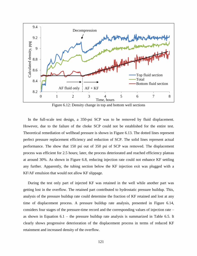
121
Figure 6.12: Density change in top and bottom well sections
In the full-scale test design, a 350-psi SCP was to be removed by fluid displacement.
However, due to the failure of the choke SCP could not be established for the entire test.
Theoretical remediation of wellhead pressure is shown in Figure 6.13. The dotted lines represent
perfect pressure replacement efficiency and reduction of SCP. The solid lines represent actual
performance. The show that 150 psi out of 350 psi of SCP was removed. The displacement
process was efficient for 2.5 hours; later, the process deteriorated and reached efficiency plateau
at around 30%. As shown in Figure 6.8, reducing injection rate could not enhance KF settling
any further. Apparently, the tubing section below the KF injection exit was plugged with a
KF/AF emulsion that would not allow KF slippage.
During the test only part of injected KF was retained in the well while another part was
getting lost in the overflow. The retained part contributed to hydrostatic pressure buildup. This,
analysis of the pressure buildup rate could determine the fraction of KF retained and lost at any
time of displacement process. A pressure buildup rate analysis, presented in Figure 6.14,
considers four stages of the pressure-time record and the corresponding values of injection rate –
as shown in Equation 6.1 – the pressure buildup rate analysis is summarized in Table 6.5. It
clearly shows progressive deterioration of the displacement process in terms of reduced KF
retainment and increased density of the overflow.
8.2
8.4
8.6
8.8
9
9.2
9.4
0 1 2 3 4 5 6 7 8
Cal
cula
ted d
ensi
ty,
ppg
Time, hours
Top fluid sectionTotalBottom fluid section
Decompression
AF fluid only AF + KF

122
Figure 6.13: Actual and ideal change in Ep and SCP
KF retained,% = 0.3205 m A
∆ρ qinj (6.1)
Where:
m – Pressure buildup rate, psi/hr A – tubing capacity, gal/ft
∆ρ – Density difference of KF and AF, ppg qinj – KF injection rate, gpm
Figure 6.14: Hydrostatic pressure buildup rate analysis
0
50
100
150
200
250
300
350
0
0.1
0.2
0.3
0.4
0.5
0.6
0.7
0.8
0.9
1
0 0.2 0.4 0.6 0.8 1
Wel
lhea
d S
CP,
psi
Pre
ssure
rep
lace
men
t ef
fici
ency
Volumetric displacement ratio
Actual efficiency change
Ideal efficiency increase
Actual SCP reduction
Ideal SCP reduction
1170
1190
1210
1230
1250
1270
1290
0 1 2 3 4 5 6
Pre
ssure
, psi
Time, hours
1
4
2
3
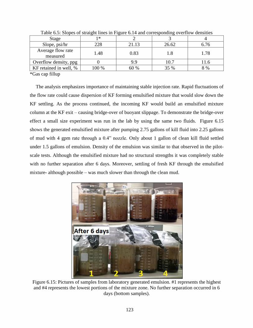
123
Table 6.5: Slopes of straight lines in Figure 6.14 and corresponding overflow densities
Stage 1* 2 3 4
Slope, psi/hr 228 21.13 26.62 6.76
Average flow rate
measured 1.48 0.83 1.8 1.78
Overflow density, ppg 0 9.9 10.7 11.6
KF retained in well, % 100 % 60 % 35 % 8 %
*Gas cap fillup
The analysis emphasizes importance of maintaining stable injection rate. Rapid fluctuations of
the flow rate could cause dispersion of KF forming emulsified mixture that would slow down the
KF settling. As the process continued, the incoming KF would build an emulsified mixture
column at the KF exit – causing bridge-over of buoyant slippage. To demonstrate the bridge-over
effect a small size experiment was run in the lab by using the same two fluids. Figure 6.15
shows the generated emulsified mixture after pumping 2.75 gallons of kill fluid into 2.25 gallons
of mud with 4 gpm rate through a 0.4” nozzle. Only about 1 gallon of clean kill fluid settled
under 1.5 gallons of emulsion. Density of the emulsion was similar to that observed in the pilot-
scale tests. Although the emulsified mixture had no structural strengths it was completely stable
with no further separation after 6 days. Moreover, settling of fresh KF through the emulsified
mixture- although possible – was much slower than through the clean mud.
Figure 6.15: Pictures of samples from laboratory generated emulsion. #1 represents the highest
and #4 represents the lowest portions of the mixture zone. No further separation occurred in 6
days (bottom samples).

124
Bridge-over of Buoyant Slippage
As discussed above, excessive or unstable injection might cause the bridge-over effect.
Another reason to be considered is fluctuation of pressure causing trapped gas expansion and
migration resulting in the flotation effect. The effects are explained below in more details.
6.4.1 Effect of Pump Pulsation
The pneumatic positive displacement pump used for KF injection generates pressure pulses
that result in fluctuation of flow rate. The flow-meter reading gave the average flow rate; but the
pump discharge pressure gauge fluctuated wildly.
Figure 6.16 shows the pump strokes per minute versus flow rate published in the pump
manual. Pulse frequency values from this figure were used for calculations. The stroking
behavior of the pump was modeled as a sinusoidal cyclic function, so the average flow rate is the
function’s integral divided by time.
Figure 6.16: Pump strokes per minute versus flow rate [Manual of Morgan Products Pump,
Model 5500DS-TR2-SR2S]
The pump discharge flow-rate fluctuation is described as,
q(t) =qmax2
sin(2πft) +qmax2
(6.2)
Integrating Equation 6.2, is,
∫ q dtt
0
= ∫ (qmax2
sin(2πft) +qmax2)dt
t
0
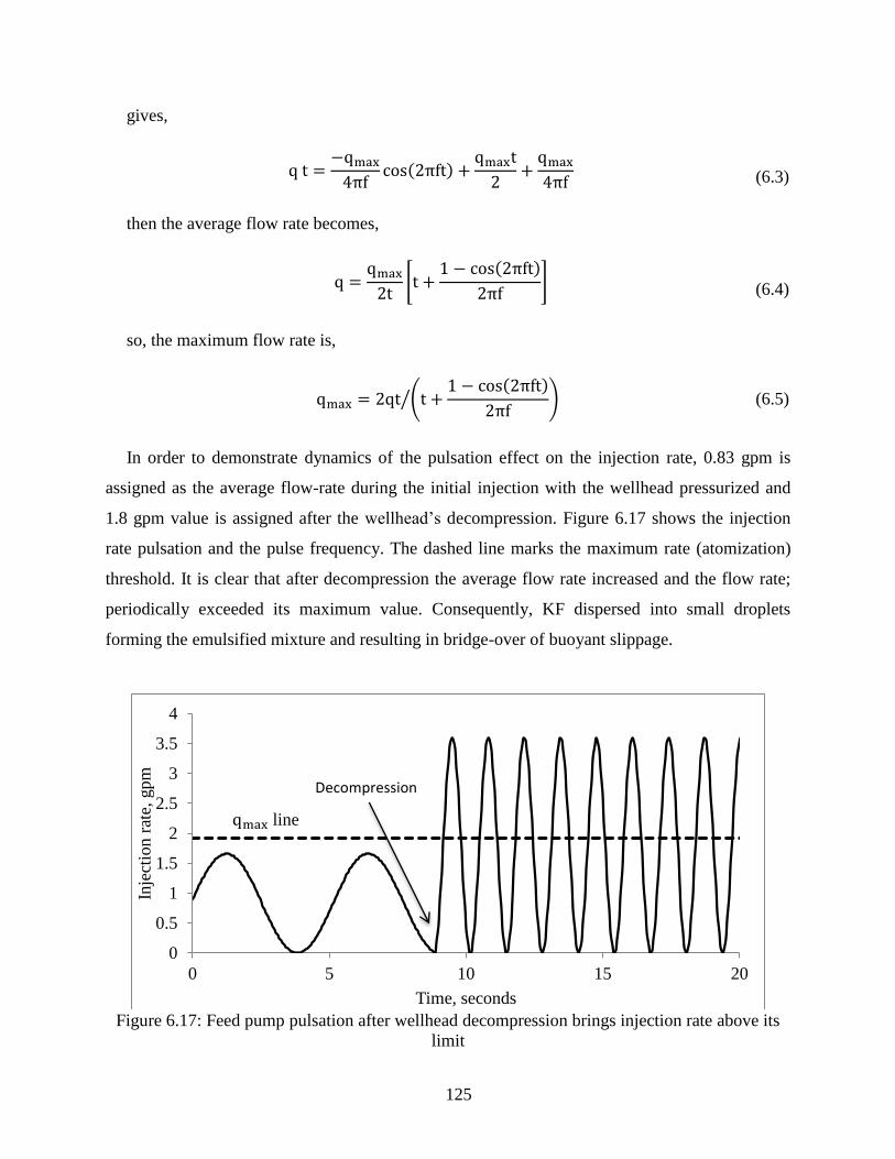
125
gives,
q t =−qmax4πf
cos(2πft) +qmaxt
2+qmax4πf
(6.3)
then the average flow rate becomes,
q =qmax2t
[t +1 − cos(2πft)
2πf] (6.4)
so, the maximum flow rate is,
qmax = 2qt (t +
1 − cos(2πft)
2πf)⁄ (6.5)
In order to demonstrate dynamics of the pulsation effect on the injection rate, 0.83 gpm is
assigned as the average flow-rate during the initial injection with the wellhead pressurized and
1.8 gpm value is assigned after the wellhead’s decompression. Figure 6.17 shows the injection
rate pulsation and the pulse frequency. The dashed line marks the maximum rate (atomization)
threshold. It is clear that after decompression the average flow rate increased and the flow rate;
periodically exceeded its maximum value. Consequently, KF dispersed into small droplets
forming the emulsified mixture and resulting in bridge-over of buoyant slippage.
Figure 6.17: Feed pump pulsation after wellhead decompression brings injection rate above its
limit
0
0.5
1
1.5
2
2.5
3
3.5
4
0 5 10 15 20
Inje
ctio
n r
ate,
gpm
Time, seconds
Decompression
qmax line

126
6.4.2 Effect of Gas Flotation
Yield point and wellhead compression cause gas entrapment in the mud. Releasing the well-
head pressure would reduce the pressure on top of trapped gas bubbles and allow them to
expand. Expanding gas bubbles would; (1) decrease the density of the fluid column, (2) start
migrating upwards. The similar phenomenon was actually tested in the pilot scale experiments.
As already shown in Figure 5.10; KF injection during gas migration results in poor displacement.
From the very beginning of the full scale test, as the kill fluid is injected and well-head pressure
increases the auto choke bled out gas; thus, a continuous but small gas expansion was present.
Nevertheless, failure of the auto choke caused decompression of the wellhead and resulted in a
drastic gas expansion, which ultimately contributed to formation of the emulsified mixture
column around the KF discharge point (bottom end of the micro-tubing).

127
CHAPTER 7: CONCLUSIONS
The objective of this study has been to understand the properties and to investigate the success
of gravity displacement of annular fluid, by a heavier fluid, to kill SCP. The following
conclusions are drawn:
Characterization of annular fluid experiments in Chapter 2 show that; in an annulus until
SCP occurs, annular fluid clears out from its weighting agents and becomes a low density
– low rheology Non-Newtonian drilling mud.
A good portion of sagged barite occupies the bottom section of the annulus. This portion
is very difficult to displace due to its high density and high rheology.
Gravity displacement of annular fluid is possible with immiscible kill fluids that have the
highest density, partitioning coefficient and interfacial tension, based on the minimum
displacement time criteria, studied in Chapter 3.
Visualization of miscible displacement experiments showed the instantaneous mixing of
heavy mud and heavy brine kill fluids right after they are injected into water. As the
annular fluid in a real-well annulus consists of water at the top, displacement becomes
impossible by using these kill fluid. When Non-Newtonian annular fluid is present,
mixing of both fluids delays but still occurs as the miscible kill fluid reaches the bottom.
Visualization experiments, documented in Chapter 4, illustrated the effect of injection
geometry on the kill fluid injection process. Side (horizontal) injection is superior to top
(vertical) injection due to advantageous effect of dissipation of jetting energy on the
casing wall, which allows higher injection rates.
For the side injection, visual inspections indicate that a narrow impinging width (rivulet
type) is required for a continuous downward movement and minimum loss of kill fluid to
overflow. For given fluids, recommended injection rate for rivulet type of impingement is
developed and presented in the study.
Vertical injection should precisely be limited since dispersion may easily occur; thus,
displacement worth nothing. Threshold injection rates for different type of fragmentation
modes are studied and given as injection rate limitations in the study. If vertical injection
through flexible tubing is desired, with given nozzle size and fluids properties, developed
limitations can be used for injection rate design.

128
Pilot scale experiments in Chapter 5 indicated the formation and structure of a mixture
zone that builds bottoms up and expands during ongoing displacement process, and has
an exponential density distribution. Based on the experimental measurements, a pressure
replacement model is developed that predicts the pressure change on top of cement in an
annulus.
The pressure replacement model is converted into dimensionless numbers by using
process measures to be used for upscaling. Correlations obtained from the experimental
data can be employed for up-scaling designs and process predictions.
Full scale test (Chapter 6) shows that when an emulsion of KF/AF forms, bridge-over
occurs and displacement process may stop. The emulsion may be formed by high
injection rate (dispersion) and/or due to concurrent movement of gas bubbles (flotation)
and kill fluid droplets.

129
CHAPTER 8: RECOMMENDATIONS
For a better estimation of displacement time, transport velocity model might be
improved. Experiments that would help for model validation could be run.
Although the well had a different geometry; the full-scale test was designed based on the
correlations obtained from the pilot tests. For a better design, displacement process in
different geometries might be better studied.
Beside the pipe and slot geometry, experiments in a transparent pilot physical annulus are
recommended to see the motion of slipping kill fluid. KF might be following a
downwards whirl motion and the droplet model could be incorrect in an annular
geometry. Seeing the phenomenon would improve or disprove study in this thesis.
In addition to water-based annular fluids, performance of immiscible buoyant
displacement in oil and synthetic based annular fluids could be tested.
The effect of brominated organics on the environment could be evaluated for any well-
size process design. Economic and environmental concerns could be compared.
Over time, any mud column creates a free-water layer on its top. Injecting miscible kill
fluids into this column might be mixing with this free-water and not displacing the
annular fluid below it. Methods for improving this method might be investigated. Before
injecting miscible heavy fluid into the column, light but high rheology mud could initially
be injected to improve Non-Newtonian character of annular fluid. Then injecting heavy
kill fluid could achieve a rope transport due to high yield-stresses of both fluids. All these
could be experimentally and theoretically studied.

130
REFERENCES
[1]Bourgoyne, A.T., S.L. Scott, and W. Manowski. A review of Sustained Casing Pressure
Occuring on the OCS. 2000. Web. December 19, 2014.
[2]Hopman, P. Webinar on Wellbore Integrity. 2013, Society of Petroleum Engineers.
[3]Kinik, K. 2012. Risk of Well Integrity Failure Due Sustained Casing Pressure. Louisiana State
University, M.S. Thesis.
[4]Wojtanowicz, A.K., S. Nishikawa, and X. Rong. Diagnosis and Remediation of Sustained
Casing Pressure in Wells. Final Report. Baton Rouge (LA): LSU, 2001. Web. December 19,
2014.
[5]Milanovic, D. and L. Smith. 2006. A Case History of Sustainable Annulus Pressure in Sour
Wells - Prevention, Evaluation and Remediation. SPE-97597-MS proceedings of the SPE
ATW HPHT Sour Well Design, The Woodlands, TX. May 17-19, 2005.
[6]Carpenter, R.B., M.E. Gonzalez, V. Granberry, and T.E. Becker. 2004. Remediating
Sustained Casing Pressure by Forming a Downhole Annular Seal with Low-Melt-Point
Eutectic Metal. SPE-87198-MS proceedings of the IADC/SPE Drilling Conference, Dallas,
TX. March 2-4, 2004.
[7]Nishikawa, S., A.K. Wojtanowicz, and J.R. Smith. 2001. Experimental Assessment of the
Bleed-and-Lube Method for Removal of Sustained Casing Pressure. PETSOC-2001-041
proceedings of the Petroleum Society's Canadian International Petroleum Conference,
Calgary, Alberta, Canada. June 12-13, 2001.
[8]Nishikawa, S. 1999. Mechanism of Gas Migration After Cement Placement and Control of
Sustained Casing Pressure. Louisiana State University, M.S. Thesis.
[9]Frigaard, I.A. and J.P. Crawshaw. 1999. Preventing buoyancy-driven flows of two Bingham
fluids in a closed pipe – Fluid rheology design for oilfield plug cementing. Journal of
Engineering Mathematics 36(4): p. 327-348.
[10]Crawshaw, J.P. and I. Frigaard. 1999. Cement Plugs: Stability and Failure by Buoyancy-
Driven Mechanism. SPE-56959-MS proceedings of the Offshore Europe Conference,
Aberdeen, Scotland. Sept 7-9, 1999.
[11]Calvert, D.G., J.F. Heathman, and J.E. Griffith. 1995. Plug Cementing: Horizontal to
Vertical Conditions. SPE-30514-MS proceedings of the SPE Annual Technical Conference
and Exhibition, Dallas, Texas. Oct. 22-25, 1995.

131
[12]Ohnesorge, W. 1936. Formation of drops by nozzles and the breakup of liquid jets. Z.
Angew. Math. Mech. 16: p. 355-358.
[13]Multiphase Flow Handbook. ed. C.T. Crowe. 2006.
[14]Reitz, R.D. 1978. Mechanism of Breakup of Round Liquid Jets. Princeton University, Ph.D.
Dissertation.
[15]Ramalingam, S., M.D. Cloeter, B. Smith, S.C. Garrick, and W. Liu. 2013. Experimental
Investigation of Viscous Liquid Jet Transitions. proceedings of the 25th Annual Conference
on Liquid Atomization and Spray Systems, Pittsburgh, PA. May 2013.
[16]Tyler, E. 1933. Instability of liquid jets. Phil. Mag. 16: p. 504-518.
[17]Teng, H., C.M. Kinoshita, and S.M. Masutani. 1995. Prediction of droplet size from the
breakup of cylindrical liquid jets. International Journal of Multiphase Flow 21(1): p. 129-136.
[18]Rayleigh, L. 1878. On the instability of jets. Lond. Math. Soc. Proc. 10: p. 4-18.
[19]Miranda, J.M. and J.B.L.M. Campos. 1999. Impinging jets confined by a conical wall:
Laminar flow predictions. AIChE Journal 45(11): p. 2273-2285.
[20]Storr, G.J. and M. Behnia. 2000. Comparisons between experiment and numerical simulation
using a free surface technique of free-falling liquid jets. Experimental Thermal and Fluid
Science 22(1–2): p. 79-91.
[21]Morison, K.R. and R.J. Thorpe. 2002. Liquid Distribution from Cleaning-in-Place
Sprayballs. Food and Bioproducts Processing 80(4): p. 270-275.
[22]Wilson, K.C., R.R. Horsley, T. Kealy, J.A. Reizes, and M. Horsley. 2003. Direct prediction
of fall velocities in non-Newtonian materials. International Journal of Mineral Processing
71(1–4): p. 17-30.
[23]Wang, T., J.F. Davidson, and D.I. Wilson. 2013. Effect of surfactant on flow patterns and
draining films created by a static horizontal liquid jet impinging on a vertical surface at low
flow rates. Chemical Engineering Science 88(0): p. 79-94.
[24]Nusselt, W. 1916. Oberflachen kondensation des Wasserdampfes. Zeitschrift Verein
Deutscher ingenieure 60: p. 569-575.
[25]Bourgoyne, A.T., M.E. Chenevert, K.K. Millheim, and F.S. Young. Applied Drilling
Engineering. SPE Textbook. Vol. 2. 1984.

132
[26]Dedegil, M.Y. 1987. Drag Coefficient and Settling Velocity of Particles in Non-Newtonian
Suspensions. Journal of Fluids Engineering 109(3): p. 319-323.
[27]Valentik, L. and R.L. Whitmore. 1965. The Terminal Velocity of spheres in Bingham
Plastics. Brit. J. Appl. Phys. 16: p. 1197-1203.
[28]Krishna, P.M., D. Venkateswarlu, and G.S.R. Narasimhamurty. 1959. Fall of Liquid Drops
in Water. Terminal Velocities. Journal of Chemical & Engineering Data 4(4): p. 336-340.
[29]Abdelouahab, M. and R. Gatignol. 2011. A new approach for computation of drop terminal
velocity in stagnant medium. Chemical Engineering Science 66(8): p. 1523-1535.
[30]Clift, R. and J.R.G.a.M.E. Weber. Bubbles, Drops and Particles. 1978, Academic Press,
INC.
[31]Bozzano, G. and M. Dente. 2009. Single Bubble and Drop Motion Modeling. proceedings of
the AIDIC Conference Series, 2009.
[32]Gordon, C., S. Lewis, and P. Tonmukayakul. 2008. Rheological Properties of Cement
Spacer: Mixture Effects. AADE-08-DF-HO-09 proceedings of the AADE Fluids Conference
and Exhibition, Houston, TX. April 8-9, 2008.
[33]Erge, O., M.E. Ozbayoglu, S.Z. Miska, M. Yu, N. Takach, A. Saasen, and R. May. 2014.
Effect of Drillstring Deflection and Rotary Speed on Annular Frictional Pressure Losses.
Journal of Energy Resources Technology-Transactions of the Asme 136(042909-1).
[34]Griffin, T.J. and W.L. Crowe. 1977. Water-Base Spacer Increases Success Ratio Of Cement
Jobs In Illinois Basin. SPE-6489-MS proceedings of the SPE/AIME Midwest Gas Storage
and Production Symposium, Indianapolis, Indiana. April 13-15, 1977.
[35]Nelson, E.B. Well Cementing. 1990: Schlumberger Educational Services.
[36]Griffin, T.J. and L.K. Moran. Spacer Composition and Method of Use. U.S. Patent.
4,083,407. Feb. 7, 1977. Print.
[37]Erge, O., E.M. Ozbayoglu, S.Z. Miska, M. Yu, N. Takach, A. Saasen, and R. May. 2014.
The Effects of Drillstring Eccentricity, Rotation, and Buckling Configurations on Annular
Frictional Pressure Losses While Circulating Yield Power Law Fluids. SPE-167950-MS
proceedings of the IADC/SPE Drilling Conference and Exhibition, Fort Worth, TX. March 4-
6, 2014.

133
[38]Brice, J.W., Jr. and B.C. Holmes. 1964. Engineered Casing Cementing Programs Using
Turbulent Flow Techniques. SPE-742-PA proceedings of the SPE Annual Gas Meeting, New
Orleans, Louisiana. Oct. 6-9, 1963.
[39]Beirute, R.M. 1976. All Purpose Cement-Mud Spacer. SPE-5691-MS proceedings of the
Society of Petroleum Engineers of AIME Symposium on Formation Damage Control,
Houston, Tx. Jan 29-30, 1976.
[40]Benge, G. 1990. Field Study of Offshore Cement-Spacer Mixing. SPE Drilling Engineering
SPE-19864-PA.
[41]Shah, S.N., N.H. Shanker, and C.C. Ogugbue. 2010. Future Challenges of Drilling Fluids
and Their Rheological Measurements. AADE-10-DF-HO-41 proceedings of the AADE Fluids
Conference and Exhibition, Houston, TX. April 6-7, 2010.
[42]Ehrhorn, C. and A. Saasen. 1996. Barite Sag in Drilling Fluids. 4(Annual Transactions of the
Nordic Rheology Society).
[43]Parvizinia, A., R.M. Ahmed, and S.O. Osisanya. 2011. Experimental Study on the
Phenomenon of Barite Sag. IPTC-14944-MS proceedings of the IPT Conference, Bangkok,
Thailand. Feb 7-9, 2014.
[44]Makinde, F.A., A.D. Adejumo, C.T. Ako, and V.E. Efeovbokhan. 2011. Modelling the
Effects of Temperature and Aging Time on the Rheological Properties of Drilling Fluids.
Petroleum & Coal 53: p. 167-182.
[45]Erge, O. 2013. Effect of Free Drillstring Rotation on Frictional Pressure Losses. University
of Tulsa, M.S. Thesis.
[46]Zamora, M. 2009. Mechanisms, Measurement And Mitigation Of Barite Sag. OMC-2009-
105 presented at the Offshore Mediterranean Conference, Ravenna, Italy. Mar 25-27, 2009.
[47]Scott, P.D., M. Zamora, and C. Aldea. 2004. Barite-Sag Management: Challenges,
Strategies, Opportunities. SPE-87136-MS proceedings of the IADC/SPE Drilling Conference,
Dallas, TX. Mar 2-4, 2004.
[48]Paslay, P., U.B.R. Sathuvalli, and M.L. Payne. 2007. A Phenomenological Approach to
Analysis of Barite Sag in Drilling Muds. SPE-110404-MS proceedings of the SPE Annual
Technical Conference and Exhibition, Anaheim, CA. Nov 11-14, 2007.
[49]Wagle, V., S. Maghrabi, and D. Kulkarni. 2013. Formulating Sag-Resistant, Low-Gravity
Solids-Free Invert Emulsion Fluids. SPE-164200-MS proceedings of the SPE Middle East Oil
and Gas Show and Conference, Manama, Bahrain. March 10-13, 2013.

134
[50]Baldock, T.E., M.R. Tomkins, P. Nielsen, and M.G. Hughes. 2004. Settling velocity of
sediments at high concentrations. Coastal Engineering 51(1): p. 91-100.
[51]Boycott, A.E. 1920. Sedimentation of Blood Corpuscles. Nature 104: p. 532.
[52]Hanson, P.M., T.K. Trigg, Jr., G. Rachal, and M. Zamora. 1990. Investigation of Barite
"Sag" in Weighted Drilling Fluids in Highly Deviated Wells. SPE-20423-MS proceedings of
the SPE 65th Annual Technical Conference and Exhibition, New Orleans, LA. Sept 23-26,
1990.
[53]Saasen, A., D. Liu, and C.D. Marken. 1995. Prediction of Barite Sag Potential of Drilling
Fluids From Rheological Measurements. SPE-29410-MS proceedings of the SPE/IADC
Drilling Conference, Amsterdam, The Netherlands. Feb 28-Mar 2, 1995.
[54]Skalle, P., K.R. Backe, S. Lyomov, and J. Svven. 1999. Barite Segregation In Inclined
Boreholes. Journal of Canadian Petroleum Technology PETSOC-97-76 38(13): p. 97-76.
[55]Moran, L.K. and K.O. Lindstrom. 1990. Cement Spacer Fluid Solids Settling. SPE-19936-
MS proceedings of the IADC/SPE Drilling Conference, Houston, TX. Feb 27-Mar 2, 1990.
[56]Wojtanowicz, A.K., S.D. Field, and Z. Krilov. 1989. Statistical Assessment and Sampling of
Drilling-Fluid Reserve. SPE Drilling Engineering SPE-17245-PA: p. 162-170.
[57]Suckling, T.P., C. Lam, S.A. Jefferis, and C.J. Pantling. 2011. Evaluation of Causes of
Bleeding of Free Water From Bentonite Slurry. proceedings of the 36th Annual Conference
on Deep Foundations, Boston, Massachusetts.
[58]Bol, G.M. 1986. Bentonite Quality and Quality-Evaluation Methods. SPE-13454-PA
proceedings of the IADC/SPE Drilling Conference, New Orleans. Aug, 1985.
[59]Abshire, L., S. Hekelaar, and P.C. Desai. 2013. Offshore Plug & Abandonment: Challenges
and Technical Solutions. OTC23906 proceedings of the Offshore Tehnology Conference,
Houston, TX. May 6-9, 2013.
[60]Hayden, R., C. Russell, A. Vereide, P. Babasick, P. Shaposhnikov, and D. May. 2011. Case
Studies in Evaluation of Cement with Wireline Logs in a Deep Water Environment.
proceedings of the SPWLA 52nd Annual Logging Symposium, Colorado Springs, CO. May
14-18, 2011.
[61]Shaposhnikov, P. and D. Findlater. 2013. Advanced Techniques in Integrated Cement
Evaluation. proceedings of the SPWLA 54th Annual Logging Symposium, New Orleans, LA.
June 22-26, 2013.

135
[62]Schlumberger "Isolation Scanner Brochure". 2011.
[63]Shaposhnikov, P. 2014. Current and New Developments in the Cement Evaluation
Technologies. presented at the Well Integrity & Asset Digitalization Conference, Houston,
TX. April 15-16, 2014.
[64]Amani, M., M. Al-Jubouri, and A. Shadravan. 2012. Comparative Study of Using Oil-Based
Mud Versus Water-Based Mud in HPHT Fields. Advances in Petroleum Exploration and
Development 4(2): p. 18-27.
[65]Wojtanowicz, A.K. and J. Yawen Ye. 1998. Environmental Control of Drilling Mud
Discharge Through Dewatering in Cold Weather Climates: Effect of Ambient Temperature.
Canadian Petroleum Technology 37(5): p. 35-40.
[66]Anifowoshe, O.L. and S.O. Osisanya. 2012. The Effect of Equivalent Diameter Definitions
on Frictional Pressure Loss Estimation in an Annulus with Pipe Rotation. SPE-151176-MS
proceedings of the SPE Deepwater and Completions Conference and Exhibition, Galveston,
Texas. June 20-21, 2012.
[67]Langlinais, J.P., A.T. Bourgoyne, Jr., and W.R. Holden. 1983. Frictional Pressure Losses for
the Flow of Drilling Mud and Mud/Gas Mixtures. SPE-11993-MS proceedings of the SPE
58th Annual Technical Conference and Exhibition, San Francisco, CA. Oct 5-8, 1983.
[68]Munson, B.R., D.F. Young, T.H. Okiishi, and W.W. Huebsch. Fundementals of Fluid
Mechanics. 6 ed. 2009.
[69]Lin, S.P. and R.D. Reitz. 1998. Drop and Spray Formation from a Liquid Jet. Annual Review
of Fluid Mechanics 30(1): p. 85-105.
[70]Alba, K., S.M. Taghavi, J.R. de Bruyn, and I.A. Frigaard. 2013. Incomplete fluid–fluid
displacement of yield-stress fluids. Part 2: Highly inclined pipes. Journal of Non-Newtonian
Fluid Mechanics 201(0): p. 80-93.
[71]Wilson, D.I., B.L. Le, H.D.A. Dao, K.Y. Lai, K.R. Morison, and J.F. Davidson. 2012.
Surface flow and drainage films created by horizontal impinging liquid jets. Chemical
Engineering Science 68(1): p. 449-460.
[72]Richardson, J.F. and W.N. Zaki. 1954. The fall velocities of spheres in viscous fluids. Trans.
Inst. Chem. Eng. 32: p. 35-41.
[73]Di Felice, R. 1994. The voidage function for fluid-particle interaction systems. International
Journal of Multiphase Flow 20: p. 153-162.

136
[74]Kaneda, Y. 1986. The drag on a sparse random array of fixed spheres in flow at small but
finite Reynolds number. Journal of Fluid Mechanics 167: p. 455-463.
[75]Koch, D.L. and A.S. Sangani. 1999. Particle pressure and marginal stability limits for a
homogenous monodisperse gas fluidized bed: kinetic theory and numberical calculations.
Journal of Fluid Mechanics 400: p. 229-263.
[76]Koch, D.L. and R.J. Hill. 2001. Inertial effects in suspension and porous media flows.
Annual Review of Fluid Mechanics 33: p. 619-647.
[77]Wen, C.Y. and Y.H. Wu. 1966. Mechanics of fluidization. Chem. Eng. Prog. Symp. Ser. 62:
p. 100-125.

137
APPENDIX A: SELECTION OF KILL FLUID DERIVATION
Rearranging Equation 3.5 by substituting Equations 3.6, 3.7 and 3.8 gives,
ϑA =
2(σg∆ρ ρf2⁄ )1 4⁄
[
1 +
(
82 (
ρf ϑL82 μf
dp√1 − αp2) μf
ρf αpm ϑL d
)
2
] 1 2⁄
Or,
ϑA = 2
{
√σg∆ρ
ρ𝑓
[
1 +
(
dp√1 − αp2
αpm d
)
2
]
⁄
}
1 2⁄
(A.1)
Using peak diameter (Equation 3.10) in place gives,
ϑA = 2 {√σg∆ρ
ρf[1 + (
1.311
αpm√σ(1 − αp2)
g ∆ρ)
2
1
d2]⁄ }
1 2⁄
(A.2)
Grouping the parameters as,
a = (1.311
αpm√σ(1 − αp2)
g ∆ρ)
2
b = (√σg∆ρ ρ𝑓⁄ )1 2⁄
so, Equation A.2 becomes,
ϑA =
2b
√1 +ad2
(A.3)
Substituting Equation A.3 into 3.13 gives the displacement time as,
tdA =ha
120 b √1 +
a
d2 (1 + 1.91
Aa d2
)

138
Or,
tdA =
ha120 b
(√d2 + a
d+ 1.91 Aa
√d2 + a
d3 ) (A.4)
Equation A.4 represents the displacement time for the droplet sizes generated below the peak
diameter. Same derivation is employed for Part B. Rearranging Equation 3.11 gives,
ϑB =1
√2 αpm ρf[g ∆ρ d2 + 8 αpm
2 σ
d]
1 2⁄
(A.5)
Grouping the parameters as,
c = √2 αpm ρf e = g ∆ρ f = 8 αpm2 σ
Equation A.5 becomes,
ϑB =
1
c[e d2 + f
d]
1 2⁄
(A.6)
Substituting Equation A.6 to 3.14 gives the displacement time for Part B as,
tdB =
1
60
hac √d
√e d2 + f(1 + 1.91
Aa d2
)
Or,
tdB =
hac
60(
√d
√e d2 + f+ 1.91 Aa
d−3 2⁄
√e d2 + f) (A.7)
In order to minimize displacement time, the roots of the derivatives of functions A.4 and A.7
should be found.
dtdAdt
= 0 dtdBdt
= 0
Taking derivative of Equation A.4:
tdA′ =
ha120 b
[1
√d2 + a−√d2 + a
d2+ 1.91 Aa (
1
d2√d2 + a− 3√d2 + a
d4 )]

139
Yields,
d2(a + 3.82Aa) + 5.73 Aaa
d4 √d2 + a= 0
d2(a + 3.82Aa) + 5.73 Aaa = 0 Gives, d = √−5.73Aaa
a+3.82Aa
Where, Aa > 0 and a >0.
Thus,
1 d4⁄ = 0 Gives, d = ∓∞
1 √d2 + a⁄ = 0 Gives, d = ∓∞
Above derivations mean that for Part A has no real roots for maximum or minimum
displacement time.
Taking derivative of Equation 3.21:
tdB′ =
hac
60 (e d2 + f )( √d √e d2 + f
2 d−
e d2√d
√e d2 + f−3 ∗ 1.91 Aa√e d
2 + f
2 d2 √d−
1.91 Aae
√d√e d2 + f)
Since ed2 + f > 0,
(e d2 + f )(0.5 d2 − 2.865 Aa) − e(d4 + 1.91Aa)
d52 √e d2 + f
= 0
Since d > 0,
(e d2 + f )(0.5 d2 − 2.865 Aa) − e(d4 + 1.91Aa) = 0
Or,
0.5 e d4 + (2.865 Aa e − 0.5 f)d2 + (2.865 Aa f + 1.91 Aa e) = 0
It can be proved that for most practical values of Aa, e and f, the expression (2.865 Aa e −
0.5 f) > 0, so the LHS>0 and the equation has no roots.

140
Calculating delta as,
∆= (2.865 Aa e − 0.5 f)2 − 4 ∗ 0.5 e (2.865 Aa f + 1.91 Aa e)
Or,
∆= 4.38 Aa2 e2 − 8.595 Aa e f + 0.25 f
2
So the roots are of variable (d2) are,
d2 =−(2.865 Aa e − 0.5 f) ∓ √4.38 Aa2 e2 − 8.595 A2 e f + 0.25 f2
e
or the “d” roots are,
d1 = √−(2.865 Aa e − 0.5 f) + √4.38 Aa2e2 − 8.595 Aa e f + 0.25 f2
e
d2 = √−(2.865 Aa e − 0.5 f) − √4.38 Aa2e2 − 8.595 Aa e f + 0.25 f2
e
d3 = −√−(2.865 Aa e − 0.5 f) + √4.38 Aa2e2 − 8.595 Aa e f + 0.25 f2
e
d4 = −√−(2.865 Aa e − 0.5 f) − √4.38 Aa2e2 − 8.595 Aa e f + 0.25 f2
e
Since the droplet size must be positive, d3 and d4 are not real. The other two roots, d1 and d2,
are also imaginary as shown by the following example.
Considering,
e = g ∆ρ = 981cm
s2∗ 1.8
gr
cm3 = 1736 f = 8 αpm2 σ = 8 ∗ 0.8712 ∗ 40.6
dyn
cm= 283
A = 130 cm2
Thus roots become,
d1 = 10 √−1 and d2 = 25 √−1
In conclusion, the displacement time function in regions A and B have no minimum value and
are monotonically decreasing, so the minimum time tdminimum = td(dmax)

141
APPENDIX B: PRESSURE REPLACEMENT MODEL DERIVATION
Displacement process involves injection of kill fluid and overflow of displaced fluid, and can
mathematically be derived from material balance equation.
ma(t) = maf +min(t) − mof(t) (B.1)
Where, ma is changing mass in annulus, maf is mass of annular fluid initially in annulus, min
is mass injected into annulus and mof is mass displaced (overflowed).
Injection rate and density of kill fluid does not change in time.
min(t) = ∫q(t) ρ(t) dt
t
0
= q ρkf t (B.2)
If both fluids inside the annulus are incompressible, outflow rate should be equal to injection
rate. The outflowing fluid mass can be represented in three separate sections: displacement of
clean annular fluid, displacement of mixture zone and displacement of clean kill fluid.
Displacement of clean annular fluid:
mofAF(t) = q∫ ρaf dt
t
0
= q ρaf t for 0 < t < tL (B.3)
Displacement of mixture:
mofmixture(t) = q∫ ρof(t) dt
t
0
for tL < t < tu (B.4)
Displacement of kill fluid:
mofKF(t) = q∫ ρkf dt
t
0
= q ρkf t for tu < t (B.5)
Substituting Equation 5.8 to Equation B.4 gives,

142
mofmixture(t) = q∫ [ρaf + (ρkf − ρaf) exp (−
q
Aatu) exp (
q
Aat) ] dt
t
0
Considering,
∫ exp (q
Aat)
t
0
=aA
q [ exp (
q
Aat) − 1]
Equation B.4 becomes,
moutmixture(t) = qρaft + aA(ρkf − ρaf) exp (−
q
Aatu) [ exp (
q
Aat) − 1] (B.6)
Thus, mass balance in the annulus (Equation B.1) for all three sections become,
During displacement of clean annular fluid, the annulus mass is,
ma(t) = maf + q (ρkf − ρaf ) t (B.7)
During charge of mixture zone, the annular mass is,
ma(t) = maf + q (ρkf − ρaf) t
− aA(ρkf − ρaf) exp (−q
Aatu) [ exp (
q
Aat) − 1]
(B.8)
At the end of mixture zone discharge, the annular mass is constant and equal to the mass of
KF, ma(t) = mkf = constant. Where, maf and mkf represent annular fluid mass full of annular
and kill fluids, respectively.
In order to derive the mass balance equations to represent pressure build-up; a few
assumptions must be made:
The minor losses of small kill fluid particles to counter-current flow are negligible.
From the moment when mixture appears in the overflow, vertical density distribution
above the top of clean kill fluid in annulus remains unchanged.
The top of clean kill fluid section will always reach the overflow port and complete
displacement will always be established by pumping necessary amount of kill fluid.

143
Using pressure data obtained from the bottom transducer is possible by converting mass
balance principle to pressure difference equation. Pressure at the bottom of annulus is related to
fluid weight as,
Pba = mgh =Vaρg
A=ma
Ag
Or, in field units,
Pba = 0.052ma
A (B.9)
Substituting Equation 5.20 to mass balance equations gives the pressure increase
functions. Density differential is grouped as ∆ρ = ρkf − ρaf.
After converting fluid mass to hydrostatic bottom pressure, mathematical model of the
pressure replacement process is developed as follows.
For displacement of annular fluid:
Pba(t) = Paf + 0.052q
A ∆ρ t for
0 ≤ t ≤ tL
(B.10)
0 ≤ P ≤ PL
For discharge of mixture zone, stage,
Pba(t) = PL +0.052 q ∆ρ
A(t − tL)
− 0.052 a ∆ρ exp (−q
Aa(tu − tL)) [ exp (
q
Aa(t − tL)) − 1]
(B.11)
for tL ≤ t < tu and PL ≤ P < Pe.
After the mixture zone discharge, ultimate pressure, Pu, is reached.
Where,
Pba – Bottom pressure, psi Paf – Initial pressure in annulus, psi
PL – Pressure when linear increase ends q – Injection rate, gpm
t – Time, min tL – Time when linear increase ends, min

144
a – Exponential coefficient, ft A – Annular capacity, gal/ft
∆ρ – Density difference of fluids, ppg tu – Ultimate time: end of displacement, min
Pu – Ultimate pressure tu, psi
Equation B.10 gives Paf when t=0 and Equation B.11 gives PL when t=tL. Based on the single
complete run, (Batch 31 shown in Figure 5.7), all the experiments are assumed as they would
reach to the complete displacement line. Thus, Equation B.11 should give the ultimate pressure
when the complete displacement is established and ultimate time of displacement has elapsed.
Hydrostatic pressure at the bottom when annular column is filled with only kill fluid is,
Pu = 0.052
VaA ρkf (B.12)
Plugging tu into Equation B.11 gives,
Pu = Pba(tu) = PL +0.052
Aq∆ρ (tu − tL)
− 0.052 a ∆ρ exp (−q
Aa(tu − tL)) [ exp (
q
Aa(tu − tL)) − 1]
Note that Equation B.11 for t=tu relates (typically unknown) mixture zone parameter “a” to
the measured values of tL and tu, as,
Pu = PL + 0.052∆ρ [
q
A(tu − tL) − a + a exp (−
q
Aa(tu − tL))] (B.13)
Equation B.13 above represents the relationship between two unknowns; ultimate time of
displacement and mixture zone density distribution coefficient (exponential coefficient). When
all the other variables are known, the equation can be solved iteratively to find tu.
Pressure replacement is transformed into dimensionless forms by using performance
measures.
Considering,

145
Pu − Paf = 0.052 (ρkf − ρaf)ha (B.14)
Pressure replacement efficiency becomes,
Ep =Pba − PafPu − Paf
=Pba − Paf0.052 ∆ρ ha
(B.15)
Also displacement ratio yields,
R =
qt
Va=
qt
haA (B.16)
Thus,
ha =
qt
R A (B.17)
Rearranging Equation B.10, substituting Equation B.17, and dividing by Equation B.14 gives,
Pba − PafPu − Paf
=0.052∆ρ
qtA
0.052 (ρkf − ρaf)ha
Considering Equations B.15 and B.16; above formula becomes,
Ep = R
Substituting Equation B.10 to B.12 when t=tL gives,
Pba − Paf = 0.052∆ρ { q
At − a exp (−
q
Aa(tu − tL)) [ exp (
q
Aa(t − tL)) − 1]}
Dividing sides by B.14 and substituting Equations B.15 and B.16 gives,
Ep = R −a
ha exp (−
haa(Ru − RL)) [ exp(
haa(R − RL)) − 1]
As learned from the slot model experiments and also mentioned in chapter 5.3 , a minor kill
fluid loss during the injection is inevitable. Similar suggestion applies to ultimate displacement
rate and pressure replacement efficiency. If the entire annular column is displaced with kill fluid,
final efficiency should give one; however, in fact, some kill fluid may be trapped in the annular

146
fluid column and 100% efficiency cannot be established. Nevertheless, neither the minor losses
nor the trapped fluid is considered in the pressure build-up model.
In dimensionless formulation, using the process performance measures, Ep and R – defined
above, the pressure replacement model becomes as follows.
For displacement of annular fluid (linear pressure increase), 0 ≤ R ≤ RL and 0 ≤ Ep ≤ EpL;
Ep(R) = R =Vp
Va=
qt
haA
For mixture zone discharge stage, RL ≤ R ≤ Ru or EpL ≤ Ep ≤ 1;
Ep(R) = R −
a
ha exp (−
haa(Ru − RL)) [ exp(
haa(R − RL)) − 1] (B.18)
After the mixture zone discharge (R ≥ Ru),
Ep(R) = 1
Note that for ultimate displacement ratio, Equation 5.14 equals unity and relates the
(typically) unknown mixture zone parameter “a” to the measured values of RL and Ru from the
tests, as,
E(Ru) = 1 = Ru −a
ha exp (−
haa(Ru − RL)) [ exp(
haa(Ru − RL)) − 1]
Solving for RL gives,
RL =a
haln (1 −
haa(Ru − 1)) + Ru (B.19)

147
APPENDIX C: PILOT-SCALE MISCIBLE DISPLACEMENT RUN
According to slot model experiments, when AF is water displacement is almost impossible.
However, when a viscous but low density AF is present, a rope transport of heavy-mud KF is
possible. To observe the phenomenon in a longer column, similar experiment was conducted in
the 20-foot pilot model. AF0903 and AF1303 (notations and properties are given in pilot scale
chapter) were used as the AF and KF, respectively. Flow rate was about 1 gpm and 45.4 gallons
of heavy mud was injected into the model for the test.
After pumping about 33 gallons of heavy mud (tu = 33 min, Ru = 1.6), bottom pressure
approached to the complete displacement line (Ep ≈ 1) - shown in Figure C.1. Bottom pressure
increased almost linearly for about 15 minutes and then the overflow density started to increase,
which indicated the mixture zone.
This single heavy-mud displacement run validates the statements in the visualization chapter.
Heavy-mud KF – when injected into a viscous AF – is able to travel downwards with little
mixing. But – once the bottom is reached – mixing starts and complete displacement is delayed
despite the low injection rate. In conclusion, even if the fluid in the annulus is viscous (which is
not expected considering the characterization of AF experiments), efficiency of the miscible
displacement in thousands of feet annulus is still indefinite.
Figure C.1: Pressure plot of heavy mud kill fluid displacement. (Batch#34)
8.5
9.5
10.5
11.5
12.5
13.5
0 5 10 15 20 25 30 35
Bott
om
Pre
ssure
, psi
Time, minutes
Complete displacement line
Mixture zone displacement

148
APPENDIX D: SOFTWARE SCRIPTS
Injection rate design function (Matlab)
function [vt, Re, Cd, qmax]= FlowRate(yp, denkf, denaf, visaf, viskf, ift, a, C)
%Density difference
dendiff=denkf-denaf;
%Viscosity ratio
visr=visaf/viskf;
%Eotvos number
Eo=0.46;
%Morton number
Mo=8.2/10^5*dendiff*visaf^4/denaf^2/ift^3;
%Variables dependent on C
numC=length(C);
vt=zeros(numC,1);
Re=zeros(numC,1);
Cd=zeros(numC,1);
qmax=zeros(numC,1);
%Grouped constants
Refix=130*denaf/visaf*sqrt(ift/dendiff);
Cdfix1=48*(3/2+visr)/(1+visr)*(1+12*Mo^(1/3))/(1+36*Mo^(1/3));
Cdfix2=0.9*Eo^(1/2)/(1.4*(1+30*Mo^(1/6))+Eo^(3/2));
vtfix=sqrt(0.27/denaf*(1.87*sqrt(ift*dendiff)-1.01*yp));
%Iteration
tol=10^-10;
maxiter=1000;
for i=1:numC
vtest=0.5;
errvt=1;
iter=0;
while errvt>tol && iter<=maxiter
iter=iter+1;
Recal=Refix*vtest;
if Cdfix2<0.45
Cdcal=((Cdfix1/Recal)*sqrt(1+0.25*Recal)/(1+sqrt(1+0.25*Recal))+0.45)*(1-C(i,1))^(-3.7);
else
Cdcal=((Cdfix1/Recal)*sqrt(1+0.25*Recal)/(1+sqrt(1+0.25*Recal))+Cdfix2)*(1-C(i,1))^(-3.7);
end
vtcal=vtfix*sqrt(1/Cdcal);
errvt=abs(vtest-vtcal)/vtest*100;
vtest=vtcal;
end
vt(i,1)=vtcal;
Re(i,1)=Recal;
Cd(i,1)=Cdcal;
qmax(i,1)=60*a*vt(i,1)*C(i,1);
end

149
Plotting function (Matlab)
clear all
clc
%Input Data
%Yield point (lbf/100sqft)
yp=2;
%Kill and Annular Fluid Densities (ppg)
denkf=(12:2:20)';
denaf=8.6;
%Kill and Annular Fluid Viscosities (cP)
viskf=8;
visaf=5;
%Interfacial Tension (dynes/cm)
ift=30;
%Annular capacity (gal/ft)
a=0.24;
%Concentration from 0.01 to 0.99
C=(0:0.01:0.99)';
%Variables dependent on concentration
numC=length(C);
numden=length(denkf);
vt=zeros(numC, numden);
Re=zeros(numC, numden);
Cd=zeros(numC, numden);
qmax=zeros(numC, numden);
%Plotting function
for i=1:numden
[vt(:,i), Re(:,i), Cd(:,i), qmax(:,i)]= FlowRate(yp, denkf(i,1), denaf, visaf, viskf, ift, a, C);
end
ColorMatrix=[0 0 0;...
0 0.498039215803146 0;...
1 0 0;...
0.47843137383461 0.062745101749897 0.894117653369904;...
0 1 0];
figure
subplot(2,2,1)
hold on;
for i=1:numden
plot(C, vt(:,i), 'LineWidth', 2, 'Color', ColorMatrix(i,:))
end
hold off;
grid on; box on;
xlabel('KF Concentration', 'FontWeight', 'bold', 'FontSize', 10)
ylabel('Transport Velocity, ft/sec', 'FontWeight', 'bold', 'FontSize', 10)
legend('\rho_{kf}= 12', '\rho_{kf}= 14', '\rho_{kf}= 16', '\rho_{kf}= 18', '\rho_{kf}= 20')
subplot(2,2,2)
hold on;
for i=1:numden
plot(C, qmax(:,i), 'LineWidth', 2 , 'Color', ColorMatrix(i,:))
end
150
hold off;
grid on; box on;
ylabel('Corresponding Flow Rate, gpm', 'FontWeight', 'bold', 'FontSize', 10)
xlabel('KF Concentration', 'FontWeight', 'bold', 'FontSize', 10)
subplot(2,2,3)
hold on;
for i=1:numden
plot(vt(:,i), qmax(:,i), 'LineWidth', 2, 'Color', ColorMatrix(i,:))
end
hold off;
grid on; box on;
ylabel('Corresponding Flow Rate, gpm', 'FontWeight', 'bold', 'FontSize', 10)
xlabel('Transport Velocity, ft/sec', 'FontWeight', 'bold', 'FontSize', 10)
subplot(2,2,4)
axis([0 1 0 1.5 0 2.5])
hold on;
for i=1:numden
plot3(C, vt(:,i), qmax(:,i), 'LineWidth', 2, 'Color', ColorMatrix(i,:))
end
hold off;
grid on; box on;
xlabel('KF Concentration', 'FontWeight', 'bold', 'FontSize', 10)
ylabel('Transport Velocity, ft/sec', 'FontWeight', 'bold', 'FontSize', 10)
zlabel('Corresponding Flow Rate, gpm', 'FontWeight', 'bold', 'FontSize', 10)
Displacement Ratio Fit model – For empirical correlation (JMP)
Fit Model(
Y( :log10Ru ),
Effects( :log10q, :log10KF_dens, :log10AF_dens, :log10AF_yp ),
Personality( Standard Least Squares ),
Emphasis( Effect Leverage ),
Run(
:log10Ru << {Lack of Fit( 0 ), Show Prediction Expression( 1 ),
Plot Actual by Predicted( 1 ), Plot Regression( 0 ),
Plot Residual by Predicted( 1 ), Plot Effect Leverage( 1 )}
) );
)
Mixture zone exponential Coefficient Fit model (JMP)
Fit Model(
Y( :log10a ),
Effects( :log10AF_dens, :log10AF_visc, :log10q ),
Personality( Standard Least Squares ),
Emphasis( Effect Leverage ),
Run(
:log10a << {Lack of Fit( 0 ), Show Prediction Expression( 1 ),
Sorted Estimates( 1 ), Plot Actual by Predicted( 1 ), Plot Regression( 0 ),
Plot Residual by Predicted( 1 ), Plot Effect Leverage( 1 )}
) );

151
VITA
Efecan Demirci was born in Istanbul, Turkey in 1988. He received his Bachelor of Science
degree in Petroleum and Natural Gas Engineering from Istanbul Technical University. During
his undergraduate studies he taught mathematics to high school students for a living. After his
graduation in 2010 he started working for Viking International Company as a coiled tubing
engineer, participated in various well stimulation operations in Turkey and Iraq, and also played
role in importing coiled tubing technology to Turkey and translating the technology to Turkish
Language. He later got qualified for the scholarship of National Turkish Petroleum Corporation
(TPAO) to study abroad for his masters. In 2011, he proceeded to Middle East Technical
University and pursued his International Welding Engineering diploma. Then in January 2012,
he started his graduate studies at Louisiana State University. A year later, he started to work on a
joint industry R&D project investigating the viability of immiscible buoyant kill technology on
remediation of sustained casing pressure in a well annulus.