Seediscussions,stats,andauthorprofilesforthispublicationat:http://www.researchgate.net/publication/222890710

Ascalableapproachtomappingannuallandcoverat250musingMODIStimesseriesdata:acasestudyintheDryChacoecoregionofSouthAmerica.RemoteSensEnviron

ARTICLEinREMOTESENSINGOFENVIRONMENT·NOVEMBER2010

ImpactFactor:6.39·DOI:10.1016/j.rse.2010.07.001

CITATIONS

86

READS

104

4AUTHORS,INCLUDING:

MatthewClark

SonomaStateUniversity

28PUBLICATIONS1,049CITATIONS

SEEPROFILE

RicardoGrau

NationalUniversityofTucuman

88PUBLICATIONS2,205CITATIONS

SEEPROFILE

Allin-textreferencesunderlinedinbluearelinkedtopublicationsonResearchGate,

lettingyouaccessandreadthemimmediately.

Availablefrom:MatthewClark

Retrievedon:16November2015

Remote Sensing of Environment 114 (2010) 2816–2832

Contents lists available at ScienceDirect

Remote Sensing of Environment

j ourna l homepage: www.e lsev ie r.com/ locate / rse

A scalable approach to mapping annual land cover at 250 m using MODIS time seriesdata: A case study in the Dry Chaco ecoregion of South America

Matthew L. Clark a,⁎, T. Mitchell Aide b, H. Ricardo Grau c, George Riner a

a Center for Interdisciplinary Geospatial Analysis, Department of Geography and Global Studies, Sonoma State University, Rohnert Park, California, USA 94928b Department of Biology, University of Puerto Rico, PO Box 23360, Río Piedras 00931-3360, Puerto Rico, USAc CONICET, Instituto de Ecología Regional, Universidad Nacional de Tucumán, Casilla de Correo 34 (4107) Yerba Buena, Tucumán, Argentina

⁎ Corresponding author. Tel.: +1 707 664 2558.E-mail address: mateolclark@gmail.com (M.L. Clark)

0034-4257/$ – see front matter © 2010 Elsevier Inc. Aldoi:10.1016/j.rse.2010.07.001

a b s t r a c t

a r t i c l e i n f o

Article history:Received 8 December 2009Received in revised form 16 June 2010Accepted 2 July 2010

Keywords:Land cover and land use changeMODIS Enhanced Vegetation Index (EVI)Time series analysisVegetation phenologyRandom ForestsGoogle Earth interpretationDry Chaco ecoregion

Land use and land cover (LULC) maps from remote sensing are vital for monitoring, understanding andpredicting the effects of complex human–nature interactions that span local, regional and global scales. Wepresent a method to map annual LULC at a regional spatial scale with source data and processing techniquesthat permit scaling to broader spatial and temporal scales, while maintaining a consistent classificationscheme and accuracy. Using the Dry Chaco ecoregion in Argentina, Bolivia and Paraguay as a test site, wederived a suite of predictor variables from 2001 to 2007 from the MODIS 250 m vegetation index product(MOD13Q1). These variables included: annual statistics of red, near infrared, and enhanced vegetation index(EVI), phenological metrics derived from EVI time series data, and slope and elevation. For reference data, wevisually interpreted percent cover of eight classes at locations with high-resolution QuickBird imagery inGoogle Earth. An adjustable majority cover threshold was used to assign samples to a dominant class. Whencompared to field data, we found this imagery to have georeferencing error b5% the length of a MODIS pixel,while most class interpretation error was related to confusion between agriculture and herbaceousvegetation. We used the Random Forests classifier to identify the best sets of predictor variables and percentcover thresholds for discriminating our LULC classes. The best variable set included all predictor variablesand a cover threshold of 80%. This optimal Random Forests was used to map LULC for each year between2001 and 2007, followed by a per-pixel, 3-year temporal filter to remove disallowed LULC transitions. Oursequence of maps had an overall accuracy of 79.3%, producer accuracy from 51.4% (plantation) to 95.8%(woody vegetation), and user accuracy from 58.9% (herbaceous vegetation) to 100.0% (water). We attributedmap class confusion to limited spectral information, sub-pixel spectral mixing, georeferencing error andhuman error in interpreting reference samples. We used our maps to assess woody vegetation change in theDry Chaco from 2002 to 2006, which was characterized by rapid deforestation related to soybean andplanted pasture expansion. This method can be easily applied to other regions or continents to producespatially and temporally consistent information on annual LULC.

.

l rights reserved.

© 2010 Elsevier Inc. All rights reserved.

1. Introduction

Land use and land cover (LULC) maps are vital for monitoring,understanding and predicting the effects of complex human–natureinteractions that span local, regional and global scales. For example, aspatial depiction of land conversion, such as deforestation foragriculture or pastures, or incremental changes, such as forestdegradation and reforestation, are important for reducing uncertaintyin carbon stocks and emissions, developing strategies for biodiversityprotection, and understanding how globalization affects local andregional land use trends (Houghton, 2005; De Fries et al., 2007).

Assessment of rapid land use changes, such as deforestation in thetropics (Archard et al., 2002), requires frequent measurements if it isto be incorporated into management and policy decisions. Further-more, global issues span political and cultural boundaries, and so LULCmaps need to be produced with spatially and temporally consistentinformation and accuracy. To meet these requirements, we need todevelop cost-effective ways for automating the processing of satelliteimages and the production of LULC maps with high temporalresolution (Defries & Belward, 2000; Skole et al., 1997).

There is a strong tradition of using data from medium resolutionsensors (10–60 m)–especially Landsat–for mapping LULC change atlocal to national scales (Alves & Skole, 1996; Steininger et al., 2001;Roberts et al., 2002; Zak et al., 2004; Boletta et al., 2006; Killeen et al.,2007; Gasparri & Grau 2009; Huang et al., 2009). This level of spatialresolution is generally sufficient for detecting fine-scale land usepatterns. However, data costs, small image extent, cloud cover, haze,

Fig. 1. The Dry Chaco ecoregion study site. MODIS tile extents are shown as the grid, andtile numbers are given with horizontal and vertical reference numbers (e.g., h11v10).

2817M.L. Clark et al. / Remote Sensing of Environment 114 (2010) 2816–2832

and infrequent measurements can make data from medium resolutionsensors impractical for regional and global mapping (Asner, 2001;Hansen et al., 2008).

Satellites such as MODIS, SPOT-Vegetation, and MERIS offermultispectral measurements with lower spatial resolution (250 to1000 m), relatively large scenes, and near-daily coverage that allowmultiple observations in a year despite cloud coverage. Multi-temporal and multispectral analysis of these data can be used toproduce LULC maps and other land cover descriptors, such as thetiming, length and frequency of vegetation growing seasons. Severalglobal land cover maps have been produced from low resolutionsatellites: 1.1-km AVHRR (IGBP DISCover , Loveland et al., 2000; UMDGLCC, Hansen et al., 2000), 1-km SPOT-Vegetation (GLC2000,Bartholomé & Belward, 2005), 500 m and 1000 m MODIS(MOD12Q1, Friedl et al., 2002; MCD12Q1, Friedl et al., 2010), and300 m MERIS (Globcover, Bicheron et al., 2008). These map productsgenerally focus on separating natural vegetation types for globalcarbon assessment and differ by source images, spatial scale, referencedata, classification techniques and class rules, making comparisonproblematic (Herold et al., 2008). Evergreen broadleaf trees and areaswithout vegetation (snow, ice, barren) tend to be well classified, butaccuracy is poor with large pixels that mix spectral and temporalsignals from trees, shrubs and herbaceous vegetation (Herold et al.,2008). Most global maps provide “baseline” information from a singletime period (mostly circa 2000), thus precluding analysis of LULCchange using one product with consistent error. The 500 mMCD12Q1MODIS product offers annual LULC maps from 2001 to 2007, withplans to continue into the future, but these products have just beenreleased and have not been thoroughly assessed for class accuracy andchange detection (Friedl et al., 2010).

In summary, there is a lack of LULC map products at regional tocontinental scales with spatially and temporally consistent informa-tion content and error, which prevents analyses of coupled naturaland human systems across political boundaries and through time. Tosatisfy this need, we develop a scalable method for mapping annualLULC at these spatial scales. We use the Dry Chaco ecoregion in SouthAmerica as a case study; however, the main impetus for this study is alarger project focused on recent LULC change in Latin America and theCaribbean. Our method is novel in that it integrates: 1) reference datainterpreted from high-resolution imagery sampled in space and timewithin an Internet-based tool (Google Earth), 2) a flexible classifica-tion scheme based on percent cover thresholds, 3) predictor variablesthat respond to phenological variation in MODIS vegetation indextime series data, 4) annual maps produced at 250 m scale, and 5) aRandom Forests classifier that is robust in the face of heterogeneousclasses and reference data error.

2. Study area: Dry Chaco ecoregion

To develop and test our method, we worked in the Dry Chacoecoregion that spans Argentina, Bolivia and Paraguay (Olson et al.,2001). This is the second largest ecoregion in Latin America, covering790,000 km2 between 17°32′26″S and 33°52′7″S latitude and 67°43′12″W and 57°59′26″W longitude (Fig. 1), and includes the largestcontinuous neotropical dry forest (Eva et al., 2004). The ecoregion ischaracterized by a monsoonal climate with a strong seasonality (drywinters, rainy summers), but average temperature and in particularrainfall vary significantly across the area. Annual mean temperaturevaries from 18°C in the southern part of the ecoregion to 21°C in thenorth, and precipitation varies from 500 mm/year in the center to1000 mm/year in the eastern and western extremes (Minetti, 1999).The vegetation is dominated by dry forest trees and shrubs, butnatural grasslands occur in areas with sandy soils and frequent fires.Most of the ecoregion is flat, with elevation rising in the wetter,western side. Elevation above mean sea level for the ecoregioncalculated from a digital elevationmodel (see Section 2.7) had a range

of 56 to 3577 m and average of 326±289 m. Lowland areas, havingelevation below 700 m, cover 91% of the ecoregion.

Historically, much of the ecoregion has been severely degraded byextensive cattle ranching and timber and charcoal extraction. Inaddition, agriculture has occurred in the foothills of the Andes and inirrigated valleys for more than a century. Citrus plantations (mostlylemon, some grapefruit and oranges) and sugar cane are importantcrops near the Andes. In the northern humid zones there are somebanana plantations, while olives are cultivated in the drier southwest.The region also has some scattered tree plantations (pine, eucalyptusand poplar) and minor fruit orchards including blueberries, peaches,figs, and walnuts. During the last 30 years, the conversion of forest toagriculture has accelerated, mostly driven by growing global fooddemand (Grau et al., 2005). In Argentina, the majority of this newdeforestation has occurred in the wetter eastern and western parts ofthe ecoregion, where millions of hectares of Chaco forest have beenreplaced with soybeans and pastures (Gasparri & Grau, 2009).

As a consequence of its large area and rapid land use change, theecoregion has the largest carbon stock and the largest source ofemissions fromdeforestation in LatinAmericaoutside theAmazonbasin(Gasparri et al., 2008). The ecoregion is part of the Tropical/SubtropicalDry Broadleaf Forest biome,whichglobally has a high percentage of areaconverted and relatively low protection (Hoekstra et al., 2005), and ithas the largest continuous habitat for large mammals (e.g., jaguars,peccaries) outside the Amazon basin, making it important for regionalconservation (Altritcher and Boaglio, 2004; Altritcher et al., 2006;Redford et al., 1990). Given its large extent and rapid changes,developing remote sensing methods to monitor LULC is a priority fortheDryChaco. Existing studieshaveused Landsat images, coveringpartsof the ecoregion in Bolivia (Killeen et al., 2007), Paraguay (Huang et al.,2009) and Argentina (Zak et al., 2004; Boletta et al., 2006; Gasparri &Grau 2009). Methods varied from automated per-pixel classification tovisual interpretation; however, despite the lack of consistent products,all studies reported accelerated deforestation since the 1990s.

Table 1Visual criteria used for estimating percent cover of land use/land cover classes in GoogleEarth QuickBird image samples (Section 3.2). The class label of each sample, andsubsequent classification scheme for a map, was determined by a variable majoritycover threshold (Section 3.8.1).

Class Abbreviation Visual criteria

Built-up areas Built Urban and industrial buildings, infrastructureand associated roads

Water Water Lakes and large riversBare areas Bare In addition to including areas of bare soil,

which could be common in deserts, this classalso includes ice, snow, sand dunes, rock, saltflats, and dry riverbeds. Open-pit mines withexposed soil/rock are included in this class.

Agriculture Ag Agricultural fields with annual crops (e.g., sugarcane, corn, wheat, soybean, rice). Perennial crops(e.g., citrus plantations) are included in theplantation class. Crops can usually be detected byplow lines, rectilinear shapes, and nearby roadsand infrastructure. Bare soil in this context wasclassified as crops, but fallow agricultural landwas classified as herbaceous or woody.

Plantations Plant The major characteristics of plantations are:perennial vegetation and the regular spacing ofthe plants. Common examples in the Chaco arepine and eucalyptus plantations, citrus and oliveorchards, and vineyards. Roads, bare ground, orgrass within the plantation were considered aspart of the plantation.

Herbaceousvegetation

Herb This class is usually dominated by native orplanted grasses and herbs. The most commonland use in this class is cattle pasture, whichcan be distinguished by trails and watering holes.This class can be confused with agriculture butis usually more heterogeneous in color (green,gray, brown) and texture.

Woodyvegetation

Woody Trees and shrubs are the major components ofthis class. Although most areas in this class arenatural areas, woody vegetation can also occurwithin agricultural and urban regions.

Mixed woodyvegetation

MixWoody Not interpreted directly in Google Earth.Woody, Herb and Bare percent cover make upthis class (see Section 3.8.1)

2818 M.L. Clark et al. / Remote Sensing of Environment 114 (2010) 2816–2832

3. Methods

3.1. Google Earth reference data collection

We collected reference data with human interpretation of high-resolution imagery in Google Earth (GE, http://www.earth.google.com). In Latin America, most of this imagery is from Digital Globe'sQuickBird satellite. Google superimposes high-resolution images overcoarser images according to image availability, quality and date, andthe final imagemosaic is streamed to the GE application fromGoogle'sservers. The use of GE provides scalability to our method in that itshigh-resolution imagery is free to access, easy to navigate, isdistributed across the region, and can be interpreted with a consistentset of rules.

We first selected random points across the Dry Chaco ecoregion,with point centers at least 1000 m apart. Points were snapped to theclosest MODIS pixel (Section 3.4). At each pixel center, a 250×250 msquare (62,500 m2) representing the pixel was generated alongwith a4×5 internal grid of cells. Each cell covered 5% of the grid (eachinternal cell was 62.5×50 m=3125 m2). Reference sample pointsand associated grid layers were developed in the Interrupted GoodeHomolosine (IGH) projection, WGS84 datum within ArcGIS 9.2 andthen projected to the geographic coordinate system (GCS, i.e., simplecylindrical projection with latitude, longitude) within a KMZ file forviewing in GE (v4.3 to v5.0). Samples with no high-resolutionQuickBird imagery in GE were removed from the sample set. Withineach sample grid, two technician-level interpreters estimated thepercent cover of seven classes with increments of 10%: woodyvegetation (Woody), herbaceous vegetation (Herb), agriculture (Ag),plantations (Plant), built-up areas (Built), bare areas (Bare), and water(Water). Each interpreter estimated percent cover based on criteriapresented in Table 1 (mixed woody is explained below and inSection 2.8.1). Fig. 2 shows typical examples of six classes (excludingWater and MixWoody) as seen in GE QuickBird imagery with the250×250 m interpretation grid, which is slightly larger than a MODISpixel. Each interpreter was allowed to consider the larger landscapecontext around the sample in assessing component classes, but allpercent cover estimates were confined to the land cover in the samplegrid. QuickBird image date is available in GE's status bar and the yearwas recorded for each sample. Samples were then labeled with theclass that had themajority cover, one label from each technician. If thetwo class labels agreed, the estimates of class cover were averaged toprovide one estimate for the sample. If the two class labels disagreed,then the technician interpretations were discarded and an “expert”interpreter (one of the authors) estimated the sample's final percentcover, and then the majority-class label came from the expert'sestimation. A mixed woody/natural vegetation (MixWoody) class wascreated from samples with a blend ofWoody, Herb and Bare cover (seeSection 3.8.1).

Our initial interpretations with random sampling yielded 3147samples, with an overabundance of non-riparian woody vegetation. Incontrast, there were relatively few samples for bare, built, plant,water, and riparian area woody, as these areas covered a smallfraction of the landscape; and thus, we implemented a stratifiedrandom sampling approach for these areas. We first digitizedpolygons in GE for Bare, Built, Plant, Water and riparian vegetationareas with QuickBird images. Random samples were generated withinthese polygons and then interpreted using the same protocol, yieldingan additional 461 reference samples (13% of total).

3.2. Reference data accuracy assessment

Reference data collected from GE were expected to have spatialand interpretation error. Spatial error may be caused by terraindisplacement in QuickBird images that have not been orthorectified.Interpretation error could be in percent cover estimates for the seven

land cover classes or in recording QuickBird image dates. These errorsare expected to vary among interpreters (Congalton & Mead, 1983;Powell et al., 2004), and can result from disagreement on class percentcover, level of training, fatigue, and data recording errors.

To test the spatial and interpretation accuracy of our GE referencedata, we collected an independent set of points from field observa-tions. Points were collected with a Trimble GeoExplorer 3 GPSreceiver (PDOP b 6.0, N 4 satellites, and average of 70 positions perpoint) on January 2 and 3, 2009 along a highway route through theSantiago del Estero, Tucuman, and Salta provinces of NW Argentina,160 to 950 m elevation.We applied differential corrections to 18 of 62locations using a public base station (SOPAC, UNSA Salta, 24°43′38.84″S, 65°24′27.52″W); the remaining 44 locationswere not corrected dueto missing base station data. At each location, we recorded thecompass bearing and estimated distance to the center of patchesdominated by one of our land cover classes. Google Earth “place-marks”were digitized with reference to GPS field locations and notes.A 250×250 m sample grid was then generated for each placemarkand loaded into GE. Four technicians and one expert estimatedpercent cover and recorded image date for each field sample using theinterpretation criteria in Table 1 (see Section 3.6). Some GPS pointswere located at road intersections visible in GE QuickBird imagery.The point location (placemark) of the GPS receiver was digitized in GEusing detailed field notes and photographs as reference. Thedifference in IGH projected coordinates (see Section 3.4) betweenthe placemark and GPS point was then used to determine GEQuickBird spatial error in meters.

Fig. 2. Example reference samples in Google Earth for six land use/land cover classes. The grid is centered on a MODIS pixel and covers 250×250 m. Each grid cell is 5% of the totalsample area.

2819M.L. Clark et al. / Remote Sensing of Environment 114 (2010) 2816–2832

3.3. MODIS imagery

We used the MODIS MOD13Q1 Vegetation Indices 250 m product(Collection 5) for LULC classification. The product is a 16-day compositeof the highest-quality pixels from daily images and includes theNormalized Difference Vegetation Index (NDVI), Enhanced VegetationIndex (EVI), blue, red, near infrared (NIR), mid-infrared reflectance andpixel reliability (Huete et al., 2002). We focused our study on MODIStiles H12V10, H12V11, and H12V12, which covermost of the Dry Chaco(Fig. 1). Scenes fromday 289, year 2000 to day 273, and year 2008 (184,16-day scenes) were analyzed in this study. For each day, scenes werereprojected from their native Sinusoidal projection to the IGHprojection(sphere radius of 6,378,137.0 m) using nearest-neighbor resampling.The original cell size of 231.7 mwasmaintained in the reprojection. TheIGH projection is a composite, equal-area projection that is useful forcalculating area over regional to global scales. A key component of thisresearch was to have the GE sample grids and MODIS pixels cover thesame area. Ideally, theMODIS scenes should be reprojected to IGH afterclassification to minimize geolocation mismatch with GE sample grids.However, GE requires GCS and sample grids projected from thesinusoidal projection to GCS were extremely skewed, especially athigher latitudes, which added error to our percent cover estimates. Byprojecting rasters to IGH first, we could generate GE sample gridscentered onMODIS pixels thatwere relatively squarewhen projected toGCS for overlay in GE.

3.4. Temporal profiles of classes

The NDVI and EVI vegetation indices (VIs) target the red and NIRspectral regions and respond to vegetation photosynthetic pigment

concentrations (mostly chlorophyll) and structure. Detailed timeseries of these data follow the annual growth cycles–or phenology–ofvegetation found in a pixel. Fig. 3 plots the temporal profiles of EVI andNDVI for example classes shown in Fig. 2, with vertical bars indicatingthe QuickBird image date. In native Chaco forest, trees and shrubs aremostly green (leaf-on) in the wet summers, producing higher VIvalues (Fig. 3—woody). Winters are relatively dry and many trees andshrubs lose their leaves (Fig. 2—woody), causing VI values to decrease.NDVI and EVI values follow the same temporal trend, but NDVI valuesare higher. At the other extreme are bare areas, such as dry lake beds(Fig. 2—bare). There is minimal to no vegetation in these areas, and VIvalues remain fairly flat through the year (Fig. 3—bare). Built-up areashave EVI and NDVI profiles that partly follow the seasonal cycle ofprecipitation due to urban vegetation, such as trees and herbaceouslots, yet vegetation index (VI) values are relatively low (Fig. 3—built-up) due to high cover of non-photosynthetic surfaces, such as roof-tops and streets (Fig. 2—built-up). Plantations have VI profiles thatrespond to seasonal precipitation cycles, yet since they are generallyirrigated, values are relatively high in the dry winter months relativeto native forest (Fig. 3—plantation vs. woody). In this example, theplantation's temporal profile shows a steady increase in VI valuesfrom 2001 to 2008, likely the result of increasing biomass andproductivity. Herbaceous vegetation is highly variable in the DryChaco landscape and includes natural grasslands and pastures forlivestock. The QuickBird image for the herbaceous example showstrails radiating from awatering hole, indicating that the area is a cattlepasture (Fig. 2—herbaceous). As with most classes, the herbaceous VIprofiles follow seasonal precipitation, yet values are more erratic thanwoody vegetation. Agriculture in the Dry Chaco is predominantlyrain-fed, and areas with mechanized agriculture (e.g., soybeans) have

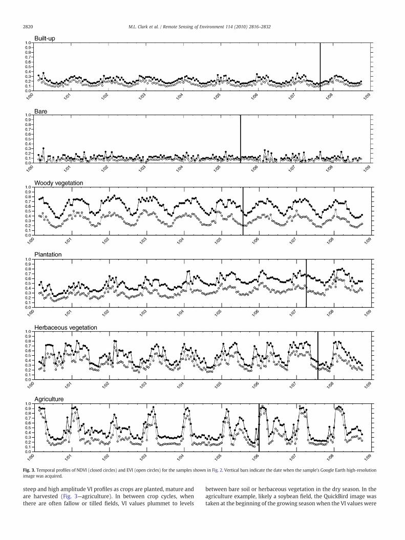
Fig. 3. Temporal profiles of NDVI (closed circles) and EVI (open circles) for the samples shown in Fig. 2. Vertical bars indicate the date when the sample's Google Earth high-resolutionimage was acquired.

2820 M.L. Clark et al. / Remote Sensing of Environment 114 (2010) 2816–2832

steep and high amplitude VI profiles as crops are planted, mature andare harvested (Fig. 3—agriculture). In between crop cycles, whenthere are often fallow or tilled fields, VI values plummet to levels

between bare soil or herbaceous vegetation in the dry season. In theagriculture example, likely a soybean field, the QuickBird image wastaken at the beginning of the growing season when the VI values were

2821M.L. Clark et al. / Remote Sensing of Environment 114 (2010) 2816–2832

increasing rapidly (Figs. 2 and 3—agriculture). The VIs in this exampletrack one growing season in 2003 and 2004, while there appear to betwo crop cycles in 2005 and 2006.

3.5. Phenological variables

We started with the assumption that land cover classes havedifferent phenological signals that can be used for automatedclassification. Our goal was to derive predictor variables from the VItime series that are sensitive to annual phenological change, yetreduce data volume and signal noise.

3.5.1. Annual statisticsWe calculated the annual statistics mean, standard deviation,

minimum, maximum and range for EVI, NDVI, red reflectance and NIRreflectance values from calendar years 2001 to 2007. The MOD13Q1pixel reliability layer was used to remove all unreliable pixels(value=3) prior to calculating statistics. We explored restrictingour analysis to highly reliable pixels (value=0), but this eliminatedtoo many data points, and so signal error from marginally reliablepixels (value=1) contributes to the total error in our process. Annualmetrics are referenced by the input band evi, ndvi, red or nir and thestatistic _mean, _stddev, _min, _max, and _range. For example,evi_mean is the mean EVI for 1 year.

3.5.2. TIMESAT processing of time series dataThe TIMESAT program (Jönsson & Eklundh, 2004) was designed to

analyze phenological signals found in time series data from satellitesensors. The program fits local functions to the time series data points,and then combines these functions into a global model. Phenologicalvariables for each growing season are then extracted from the smoothmodel function, thereby reducing the influence of signal noise in theraw data. We used TIMESAT v.2.3 (Jönsson & Eklundh, 2004) toprocess EVI and NDVI data from Julian day 289, year 2000 to Julian day273, year 2008 (23 points per years×8 years=184 points). Thistemporal window does not align with calendar years, but allowed theprogram to have ample data to fit a full function to the main SouthernHemisphere growing seasons 2001–2002 to 2007–2008. The MOD13pixel reliability band was used to weight each point in the time series:value 0 (good data) had full weight (1.0), values 1–2 (marginal data,snow/ice) had half weight (0.5), and value 3 (cloudy) had minimalweight (0.1). Function-fitting parameters used in TIMESAT were: aSavitzky-Golay filter procedure, 3- and 4-point window over 2 fittingsteps, adaptation strength of 2.0, no spike or amplitude cutoffs, seasoncutoff of 0.0, and begin and end of season threshold of 20%.

Fig. 4. Example TIMESAT function fit (black line) to 16-day MOD13 NDVI data (open circles wthe function are numbered on the figure for the 2006/2007 growing season, with variable n

An example fit to NDVI data from an agriculture sample is shownin Fig. 4. Phenological variables extracted for each growing seasonincluded: 1. length of the season (seas_length); 2. base level, averageof the left and right minimum values (base_level); 3. largest data valuefor the fitted function during the season (maximum); 4. seasonalamplitude (amplitude); 5. rate of increase at the beginning of theseason (left_der); 6. rate of decrease at the end of the season(right_der); 7. small seasonal integral (small_int); 8. large seasonalintegral (large_int); 9. number of seasons in a calendar year(num_seas); 10. time for the start of the season (day_start); 11. timefor the end of the season (day_end); and, 12. time for the mid of theseason (day_mid). A custom program was created to output thesephenological variables as raster bands in a stack for each calendaryear, 2001 to 2007. TIMESAT outputs fractions of band number forvariables 10, 11, and 12. Julian day within a calendar year (0 to 366)was linearly interpolated from a lookup table of MODIS bands andJulian day. Each image pixel was processed independently andphenological variables were labeled with the year in which theseason started. Only data for the first growing season in a calendaryear were used in our analyses. If TIMESAT failed to retrieve a growingseason for a year, the phenological variables for the year were set to ano data value.

3.6. Terrain variables

Additional auxiliary predictor variables used in the classificationincluded elevation and slope derived from the Shuttle RadarTopography Mission (SRTM) 90 m Digital Elevation Model (DEM)that had missing data filled by the Consultative Group for Interna-tional Agriculture Research (CGIAR, DEM Version 4, http://www.srtm.csi.cgiar.org). Degree slope was derived from the DEM at 90 m andthen both elevation and slope were projected to the IGH projectionusing a bilinear interpolationmethod and a 231.7 m cell size, tomatchthe MODIS-derived datasets.

3.7. Classification with Random Forests

We implemented per-pixel mapping of land cover with theRandom Forests (RF) tree-based classifier (Breiman, 2001). Decisiontree classifiers have an advantage overmore traditional classifiers, likethe maximum likelihood classifier, in that they make no assumptionsabout data distributions (e.g., normality), can handle data withdifferent scales, and can adapt to noise and non-linear relationshipsinherent in remote sensing data (Friedl & Brodley, 1997). For example,a highly variable class such as agriculture, which includes different

ith dashed line) for an agriculture pixel. TIMESAT phenological variables derived fromames and actual values in the table. See Section 3.6.2 for more information.

2822 M.L. Clark et al. / Remote Sensing of Environment 114 (2010) 2816–2832

crops, cropping patterns and fallow periods, may have multipledecision paths through a tree that all lead to the agriculture class.

The RF classifier builds multiple decision trees from bootstrappedsampling of the reference data. A final class is determined from themajority vote of the ensemble of trees—the forest. To decrease thetime it takes to construct trees, RF tests subsets of the predictorvariables for each decision branch (node). Roughly 2/3 of thereference data are sampled with replacement to build each tree,while 1/3 of the reference data are withheld from tree construction(called “out-of-bag”, or OOB samples). The OOB samples are sentdown trees for which they were not used, and the difference betweenthe predicted and actual class is used to calculate an error matrix andunbiased estimate of accuracy (Breiman, 2001). RF also trackspredictor variable importance, which is calculated as a decrease inoverall or class-level classification accuracy when the variable ispermuted in the OOB samples.

Random Forests have been used in remote sensing to map landcover (Chan & Paelinckx, 2008; Gislason et al., 2006; Pal, 2005; Sesnieet al., 2008), forest biomass and structural parameters (Baccini et al.,2004; Hudak et al., 2008), forest successional stage (Falkowski et al.,2009), habitat (Korpela et al., 2009; Martinuzzi et al., 2009) andinvasive species (Lawrence et al., 2006). In land cover studies, the RFclassifier has been found to be stable and relatively fast, involve fewuser-defined parameters and yield overall accuracies that are either

Fig. 5. Distribution of reference samples collected in Google Earth. Year corresponds to the imyear is shown in parentheses.

comparable to or better than other classifiers, such as maximumlikelihood, spectral angle mapper and conventional decision trees(Lawrence et al., 2006), AdaBoost decision trees and neural networks(Chan & Paelinckx, 2008), and support vector machines (Pal, 2005).

3.7.1. Reference data preparationAnnual statistics and TIMESAT phenology were extracted for the

year corresponding to the QuickBird image year (2002 to 2007) foreach GE reference sample. Since samples came from different years,they included variability in space and time. Sample class labels wereassigned according to the class with majority cover. Each GE samplethus included a majority class and its percent cover, and a suite ofpredictor variables: annual statistics, TIMESAT phenology and terrainvariables. This dataset was filtered to remove samples with noTIMESAT values when using EVI or NDVI. This filtered version ofsamples is called the “reference dataset”. There were 3309 totalsamples, spanning years 2002 to 2007 (Fig. 5). The spatial distributionof samples was clumped, reflecting the patchy distribution ofQuickBird scenes in Google Earth.

The reference dataset was then split by randomly selecting 70%and 30% of samples per class for training and testing, respectively,with a maximum limit of 700 samples in any given class (Table 2). Thetraining and test datasets were filtered to provide 5 datasets with 60%,80% and 100% majority cover thresholds. For example, the 60%

age date of the high-resolution imagery under a sample. Total number of samples for a

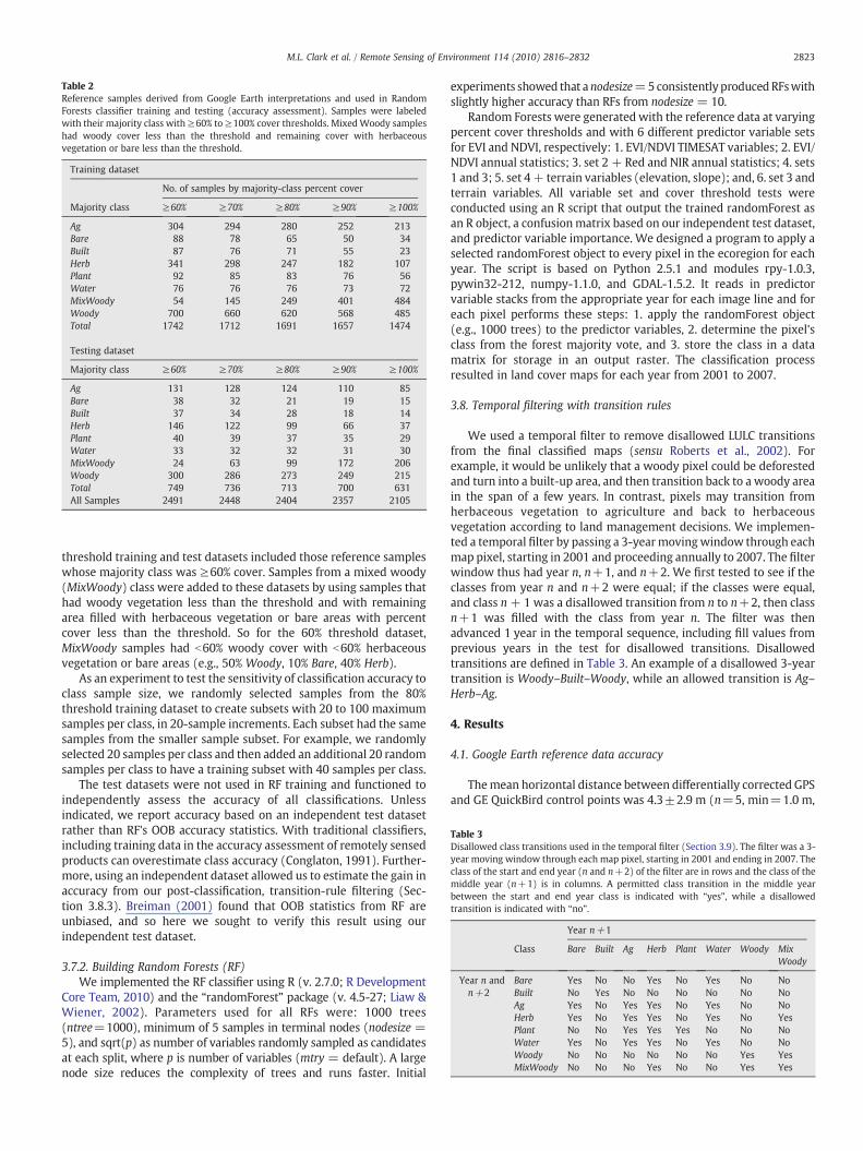
Table 2Reference samples derived from Google Earth interpretations and used in RandomForests classifier training and testing (accuracy assessment). Samples were labeledwith their majority class with≥60% to≥100% cover thresholds. MixedWoody sampleshad woody cover less than the threshold and remaining cover with herbaceousvegetation or bare less than the threshold.

Training dataset

No. of samples by majority-class percent cover

Majority class ≥60% ≥70% ≥80% ≥90% ≥100%

Ag 304 294 280 252 213Bare 88 78 65 50 34Built 87 76 71 55 23Herb 341 298 247 182 107Plant 92 85 83 76 56Water 76 76 76 73 72MixWoody 54 145 249 401 484Woody 700 660 620 568 485Total 1742 1712 1691 1657 1474

Testing dataset

Majority class ≥60% ≥70% ≥80% ≥90% ≥100%

Ag 131 128 124 110 85Bare 38 32 21 19 15Built 37 34 28 18 14Herb 146 122 99 66 37Plant 40 39 37 35 29Water 33 32 32 31 30MixWoody 24 63 99 172 206Woody 300 286 273 249 215Total 749 736 713 700 631All Samples 2491 2448 2404 2357 2105

Table 3Disallowed class transitions used in the temporal filter (Section 3.9). The filter was a 3-year moving window through each map pixel, starting in 2001 and ending in 2007. Theclass of the start and end year (n and n+2) of the filter are in rows and the class of themiddle year (n+1) is in columns. A permitted class transition in the middle yearbetween the start and end year class is indicated with “yes”, while a disallowedtransition is indicated with “no”.

Year n+1

Class Bare Built Ag Herb Plant Water Woody MixWoody

Year n andn+2

Bare Yes No No Yes No Yes No NoBuilt No Yes No No No No No NoAg Yes No Yes Yes No Yes No NoHerb Yes No Yes Yes No Yes No YesPlant No No Yes Yes Yes No No NoWater Yes No Yes Yes No Yes No NoWoody No No No No No No Yes YesMixWoody No No No Yes No No Yes Yes

2823M.L. Clark et al. / Remote Sensing of Environment 114 (2010) 2816–2832

threshold training and test datasets included those reference sampleswhose majority class was ≥60% cover. Samples from a mixed woody(MixWoody) class were added to these datasets by using samples thathad woody vegetation less than the threshold and with remainingarea filled with herbaceous vegetation or bare areas with percentcover less than the threshold. So for the 60% threshold dataset,MixWoody samples had b60% woody cover with b60% herbaceousvegetation or bare areas (e.g., 50% Woody, 10% Bare, 40% Herb).

As an experiment to test the sensitivity of classification accuracy toclass sample size, we randomly selected samples from the 80%threshold training dataset to create subsets with 20 to 100 maximumsamples per class, in 20-sample increments. Each subset had the samesamples from the smaller sample subset. For example, we randomlyselected 20 samples per class and then added an additional 20 randomsamples per class to have a training subset with 40 samples per class.

The test datasets were not used in RF training and functioned toindependently assess the accuracy of all classifications. Unlessindicated, we report accuracy based on an independent test datasetrather than RF's OOB accuracy statistics. With traditional classifiers,including training data in the accuracy assessment of remotely sensedproducts can overestimate class accuracy (Conglaton, 1991). Further-more, using an independent dataset allowed us to estimate the gain inaccuracy from our post-classification, transition-rule filtering (Sec-tion 3.8.3). Breiman (2001) found that OOB statistics from RF areunbiased, and so here we sought to verify this result using ourindependent test dataset.

3.7.2. Building Random Forests (RF)We implemented the RF classifier using R (v. 2.7.0; R Development

Core Team, 2010) and the “randomForest” package (v. 4.5-27; Liaw &Wiener, 2002). Parameters used for all RFs were: 1000 trees(ntree=1000), minimum of 5 samples in terminal nodes (nodesize =5), and sqrt(p) as number of variables randomly sampled as candidatesat each split, where p is number of variables (mtry = default). A largenode size reduces the complexity of trees and runs faster. Initial

experiments showed that anodesize=5consistentlyproducedRFswithslightly higher accuracy than RFs from nodesize = 10.

Random Forests were generated with the reference data at varyingpercent cover thresholds and with 6 different predictor variable setsfor EVI and NDVI, respectively: 1. EVI/NDVI TIMESAT variables; 2. EVI/NDVI annual statistics; 3. set 2 + Red and NIR annual statistics; 4. sets1 and 3; 5. set 4+ terrain variables (elevation, slope); and, 6. set 3 andterrain variables. All variable set and cover threshold tests wereconducted using an R script that output the trained randomForest asan R object, a confusionmatrix based on our independent test dataset,and predictor variable importance. We designed a program to apply aselected randomForest object to every pixel in the ecoregion for eachyear. The script is based on Python 2.5.1 and modules rpy-1.0.3,pywin32-212, numpy-1.1.0, and GDAL-1.5.2. It reads in predictorvariable stacks from the appropriate year for each image line and foreach pixel performs these steps: 1. apply the randomForest object(e.g., 1000 trees) to the predictor variables, 2. determine the pixel'sclass from the forest majority vote, and 3. store the class in a datamatrix for storage in an output raster. The classification processresulted in land cover maps for each year from 2001 to 2007.

3.8. Temporal filtering with transition rules

We used a temporal filter to remove disallowed LULC transitionsfrom the final classified maps (sensu Roberts et al., 2002). Forexample, it would be unlikely that a woody pixel could be deforestedand turn into a built-up area, and then transition back to a woody areain the span of a few years. In contrast, pixels may transition fromherbaceous vegetation to agriculture and back to herbaceousvegetation according to land management decisions. We implemen-ted a temporal filter by passing a 3-yearmovingwindow through eachmap pixel, starting in 2001 and proceeding annually to 2007. The filterwindow thus had year n, n+1, and n+2. We first tested to see if theclasses from year n and n+2 were equal; if the classes were equal,and class n+ 1 was a disallowed transition from n to n+2, then classn+1 was filled with the class from year n. The filter was thenadvanced 1 year in the temporal sequence, including fill values fromprevious years in the test for disallowed transitions. Disallowedtransitions are defined in Table 3. An example of a disallowed 3-yeartransition is Woody–Built–Woody, while an allowed transition is Ag–Herb–Ag.

4. Results

4.1. Google Earth reference data accuracy

Themean horizontal distance between differentially corrected GPSand GE QuickBird control points was 4.3±2.9 m (n=5, min=1.0 m,

Table 5Accuracy results for Random Forests with the 6 variable sets, excluding and includingthe MixWoody class, and a 60%, 80% and 100% cover threshold. Overall=independenttest overall accuracy; OOB=out-of-bag overall accuracy.

No MixWoody With MixWoody

Variable set Overall OOB Overall OOB

Set 160 66.5% 65.6% 64.5% 63.7%80 71.0% 68.9% 62.3% 59.8%100 76.0% 76.0% 60.2% 62.3%

Set 260 62.3% 60.1% 59.3% 57.9%80 66.6% 63.5% 58.2% 53.6%100 74.4% 72.1% 55.9% 57.5%

Set 360 74.9% 75.2% 71.6% 72.8%80 79.0% 78.8% 69.6% 69.1%100 84.9% 83.8% 69.6% 72.2%

Set 460 77.7% 76.9% 75.6% 74.0%80 82.1% 80.4% 73.1% 71.1%100 85.9% 84.9% 72.4% 74.6%

Set 560 80.3% 78.6% 77.7% 75.7%80 82.9% 82.0% 74.2% 71.7%100 86.1% 86.7% 72.9% 74.9%

Set 660 76.8% 78.1% 75.2% 76.3%80 81.6% 81.4% 71.9% 71.6%100 86.1% 84.9% 71.0% 73.7%

1. Timesat; 2. VI; 3. VI+Red+NIR; 4. VI+Red+NIR+Timesat; 5. VI+Red+NIR+Timesat+Terrain; 6. VI+Red+NIR+Terrain.

2824 M.L. Clark et al. / Remote Sensing of Environment 114 (2010) 2816–2832

max=8.6 m). However, uncorrected points had a mean horizontalerror of 14.9±13.1 m (n=16, min=1.3 m, max=43.0 m). Thissuggests that GPS horizontal position error could account for 10 m ofthe discrepancy between GPS and GE QuickBird control points. Withcorrected and uncorrected points combined, the mean horizontalerror between GPS and GE QuickBird points was 12.4±12.3 m,(n=21, min=1.0 m, max=43.0 m), which is only 5.4% of the lengthof a MODIS pixel.

Technicians agreed in their majority class interpretation of GEimages for 83% of the reference samples (Table 4, top panel).Consequently, 17% of the reference samples were reviewed by anexpert, who then determined the final class label. Techniciansdisagreed more often on Herb samples or samples that had no clearmajority cover (i.e., 50% cover by 2 classes). They had moderatedisagreement on Ag and Bare, while they had N90% agreement for theother classes. Expert and technician interpretation of the majorityclass in GE imagery had an 88% and 86% overall agreement withobservations from the field, respectively (Table 4, bottom panel). Mostof the errors were in discriminating Ag and Herb samples.

4.2. Experiments with variable sets

We first added sets of predictor variables to the RF classifier(Section 3.8.2) while adjusting the percent cover threshold. Sets withvariables based on EVI generally outperformed those based on NDVI,and so we present only results using EVI (Table 5). The overallaccuracy calculated from the RF OOB process relative to theindependent test dataset, across all variable sets and five percentcover thresholds, differed on average by −1.0±1.1% withoutMixWoody and −0.3±1.1% with MixWoody (OOB–independent);that is, the OOB and independent test accuracies were very similar,with OOB providing accuracy estimates that were on average, slightlypessimistic. In discussing results, we focus on accuracy estimatesusing the independent test dataset.

For all variable sets, overall accuracy was higher when theMixWoody class, which had spectrally mixed pixels, was excludedfrom the classification (Table 5). Overall accuracy steadily improvedwhen mixed pixels were further filtered from the classification byraising the percent cover threshold, i.e., 100% had the highest pixel“purity” (Table 5—noMixWoody). In contrast, overall accuracy tendedto decrease with a higher cover threshold when the MixWoody classwas included in the classification (Table 5—with MixWoody).

For each cover threshold, there was a steady increase in overallaccuracy with the addition of more predictor variables, with higheroverall accuracies reached with sets 4 to 6. The lowest overallaccuracies were with annual statistics (set 2), while TIMESAT

Table 4Accuracy assessment of Google Earth interpretation. The top table shows percentagreement of 2 technicians in majority cover class for reference samples (training andtesting ≥70% majority cover in Table 2). The bottom table shows agreement forsamples visited in the field. There were 4 technician-level interpreters and one expert.Error matrices were calculated for each comparison: expert against field observationsand technicians against field observations. Accuracies are percent of points inagreement for all points available (overall) or individual classes.

Reference samples with ≥70% majority cover (training and testing)

Overall Ag Built-up

Herb Plant Bare Water Woody Nomajority

Technicianagreement

83% 77% 92% 59% 96% 74% 90% 92% 48%

Agreement of expert and technicians with field observations

Overall Ag Built Herb Plant Woody

No. of samples 105 27 15 19 16 28Expert 88% 78% 100% 63% 95% 100%Tech mean 86% 63% 100% 73% 97% 100%

phenology variables (set 1) had improved accuracy. When Red andNIR annual statistics were combined with EVI annual statistics (set 3),accuracy improved on average 8.5% and 7.5% without and withMixWoody, respectively. Adding TIMESAT variables to set 3 (set 4)increased overall accuracy on average 2.3% and 3.3% without and withMixWoody, respectively. Combining set 4 variables with elevation andslope terrain variables (set 5) increased accuracy on average 1.4%without MixWoody and 1.5% with MixWoody. Finally, adding terrainvariables to annual statistics (set 4) variables, to create set 6,decreased accuracy slightly. The highest overall accuracy achievedwas 86.1% without the MixWoody class and a 100% cover threshold.The highest overall accuracy with MixWoody was 77.7%, using a 60%threshold and variable set 5, yet the user and producer accuracieswere 0.0% for MixWoody (Table 6). With the 80% cover threshold andset 5, overall accuracy was 74.2% and MixWoody user accuracyimproved substantially to 54.9% (Table 6).

For operational mapping, we sought a classifier that had arelatively high overall and class accuracy, while accommodatingmixed pixels—which are prevalent in the Dry Chaco landscape. Wethus chose a classifier with MixWoody and a relatively low coverthreshold (i.e., less pixel purity).We focused on RFswith variable set 5since they had the highest overall accuracy (Table 5). The 60%

Table 6Class producer and user accuracy results for the Random Forests classification with theMixWoody class, variable set 5 and a 60%, 80% and 100% cover threshold.

Ag Bare Built Herb Mix Woody Plant Water Woody

Class producer accuracy60 74.0% 68.4% 78.4% 67.8% 0.0% 47.5% 78.8% 95.3%80 73.4% 81.0% 78.6% 53.5% 50.5% 51.4% 78.1% 92.3%100 83.5% 80.0% 57.1% 29.7% 66.5% 27.6% 83.3% 87.4%

Class user accuracy60 82.9% 74.3% 76.3% 58.2% 0.0% 90.5% 96.3% 83.9%80 82.7% 68.0% 81.5% 47.7% 54.9% 79.2% 100.0% 84.0%100 74.0% 85.7% 80.0% 55.0% 65.6% 66.7% 100.0% 76.7%

Table 7Class user accuracy for Random Forests classifications with a maximum limit on training samples per class (see Section 3.8.1). The label “All” refers to the classification using allavailable training data (Table 2—training dataset). All accuracies were assessed with the independent dataset (Table 2—testing dataset).

Samples per class Overall Ag Bare Built Herb MixWoody Plant Water Woody

20 61.2% 71.4% 57.6% 53.2% 20.9% 39.1% 38.4% 93.1% 89.0%40 68.2% 76.4% 61.3% 60.5% 46.7% 41.9% 39.7% 100.0% 89.2%60 71.0% 80.4% 62.5% 65.9% 48.3% 45.5% 51.7% 100.0% 89.5%80 71.8% 79.3% 62.5% 66.7% 51.1% 47.6% 51.7% 100.0% 90.4%100 73.6% 84.1% 66.7% 77.1% 55.8% 47.7% 52.8% 96.2% 88.8%All 74.2% 82.7% 68.0% 81.5% 47.7% 54.9% 79.2% 100.0% 84.0%

2825M.L. Clark et al. / Remote Sensing of Environment 114 (2010) 2816–2832

threshold was excluded because it could not classify MixWoody. The100% threshold RF was also excluded because it was trained onsamples with very high pixel purity. Producer and user accuracy forMixWoody was 33.0% and 10.9% higher for the 80% threshold over anRF with a 70% threshold, respectively (data not shown). In contrast,Herb producer and user accuracy was 12.9% and 4.8% lower with the80% threshold relative to the 70% threshold, respectively (data notshown). Accuracy trends for other classes were less clear whencomparing the 70% and 80% thresholds; however, we found that the80% threshold produced more conservative maps depicting change inwoody vegetation, and so this threshold was used for subsequentanalyses (Section 4.3 to 4.5).

4.3. Sensitivity of Random Forests classifier to class sample size

Our final experiment involved adjusting themaximum sample sizeper class in the training dataset. We used an 80% cover threshold,variable set 5 (all variables) and included MixWoody. There was ageneral increase in overall and user accuracy with more samples perclass (Table 7). Overall accuracy climbed steadily with the addition oftraining samples. In general, 60 to 100 samples per class producedonly slightly lower overall map accuracy relative to using all trainingsamples. Water and Woody were well classified with only 20 trainingsamples. With 100 samples per class, the RF overall accuracy was 0.6%lower, and Ag, Herb and Woody had higher user accuracy relative tothe RF trained with all samples. In contrast, the RF with all trainingsamples had 7.2% and 26.4% higher user accuracy for MixWoody andPlant, respectively.

4.4. Final classification

Overall classification accuracy for our finalmapwas 74.2% (Table 5—set 5, 80% threshold, MixWoody). In reviewing 182 misclassifiedsamples, we found that some test samples were clearly misinterpreted.An expert re-estimated the percent cover for the 182 misclassifiedsamples without prior knowledge of the original class label or RF classprediction. A new class label was then assigned to each sample andaccuracy statistics were recalculated (Table 8). Nine test samples were

Table 8Error matrix for the final classification using all predictor variables (Set 5) with an 80% covesamples (Section 4.4).

Classification Reference

Ag Bare Built Herb MixW

Ag 96 – – 8 4Bare – 17 – 2 3Built – – 22 2 2Herb 18 – 3 63 13MixWoody 1 1 1 13 63Plant 1 – – 1 1Water – – – – –

Woody 3 – – 6 25Total 119 18 26 95 111Producer 80.7% 94.4% 84.6% 66.3% 56.8%

excluded from the revised accuracy assessment because they no longerhad N80% majority cover, nor fit into the MixWoody class. For theremaining results and discussion of the final map, we use accuracystatistics from Table 8. Class producer accuracywas lowest for Plant andhighest forWoody, while user accuracywas lowest for Herb and highestfor Water. Most Woody misclassified (omitted) samples went toMixWoody. Woody had lower user accuracy, due to misclassified(committed) Herb, MixWoody and Plant samples. Herb samples wereconfused with most classes, especially Ag and MixWoody, while mostmisclassified Ag samples were confused with Herb. Plant had lowproducer accuracymainly due to confusionwithWoody.MixWoodywasalso difficult to map. Most misclassified MixWoody samples wereconfused with Herb and Woody. The user accuracy of MixWoody washigher than its producer accuracy because samples were committedfrom Herb and Woody.

Fig. 6 shows the mean decrease in OOB overall and class produceraccuracy when a given predictor variable was withheld from the RF. Avariable that created a greater decrease in accuracy was thusconsidered to be relatively important in the RF. In terms of overallaccuracy, the most important variables were the Red mean, minimumand maximum, NIR mean and base level. The TIMESAT variables weregenerally less important than Red and NIR annual statistics. Importantvariables for discriminating Woody were similar to those for overallaccuracy. Red mean, EVI standard deviation and season length wereimportant for classifying Ag. Plantations were best separated withelevation, EVI minimum and base level. Red mean was particularlyimportant for Built accuracy, while NIR mean was important forWateraccuracy.

There were some pixels in the EVI images that did not have clearseasonality (e.g., bare areas, water), which prevented TIMESAT fromfitting a function and resulted in null values. Prior to transition-rulefiltering, we filled pixels with null TIMESAT variables with the classfrom the RF using set 6 variables, 80% cover threshold (Table 5, doesnot include TIMESAT).

We extracted the class value from our transition-rule filteredmaps(years 2001 to 2007) for the location and year of samples in the testdataset; filtered map and class values (test dataset with secondaryreview)were then compared as an errormatrix (data not shown). The

r threshold and independent test data with a secondary expert review of misclassified

oody Plant Water Woody Total User

1 1 – 110 87.3%– 3 – 25 68.0%1 – – 27 81.5%5 4 1 107 58.9%1 1 9 90 70.0%19 – 1 23 82.6%– 25 – 25 100.0%10 – 253 297 85.2%37 34 264 70451.4% 73.5% 95.8% 79.3%

Fig. 6.Mean decrease in overall and class producer accuracy from 1000 trees in Random Forests. Input predictor variables were EVI set 5 (all variables). Those variables with highermean decrease in accuracy are considered to be more important for overall or class-level classification.

2826 M.L. Clark et al. / Remote Sensing of Environment 114 (2010) 2816–2832

transition-rule filter improved overall accuracy 0.1% relative to theunfiltered maps. User accuracy increased 6.5% for Built, 0.7% for Plant,and 0.5% for Woody. Bare, Herb and Water showed no improvementwith transition-rule filtering, while Ag and MixWoody user accuracydecreased 0.8% and 1.2%, respectively.

4.5. Land use/Land cover change from 2002 to 2006

The area of LULC for the Dry Chaco ecoregion from 2002 to 2006 ispresented in Fig. 7. Note that only years 2002 through 2006 had classvalues changed by the transition-rule filter, and sowe describe changewithin those years. Woody decreased each year while Ag, Herb andMixWoody expanded (Fig. 7). From 2002 to 2006, our maps showed a

6,969,951 ha decrease inWoody, or 11.9% of the 2002 area. In contrast,Ag increased by 1,650,564 ha, Herb increased by 984,634 ha andMixWoody increased 4,392,469 ha, whichwere 44.9%, 17.5% and 55.0%increases from their 2002 area, respectively. Of the pixels that wereWoody in 2002 and another class in 2006, 68.9% went to MixWoody(5,695,721 ha), 13.3% went to Ag (1,100,303 ha) and 16.7% went toHerb (1,382,515 ha). There were also 659,233 ha of MixWoody thattransitioned into Woody between 2002 and 2006. Given the classifierconfusion of Woody and MixWoody, some of the Woody loss or gain iscertainly related tomisclassification withMixWoody; however, part ofthis change is likely related to forest degradation (e.g., Woody toMixWoody) or woody growth (e.g., MixWoody to Woody). There wasmuch less confusion between Woody and Ag or Herb samples, and

Fig. 7. Area of the Dry Chaco ecoregion covered by woody vegetation, agriculture,herbaceous vegetation, mixed woody and all other classes (plantations, water, bare,and built-up) for years 2002 to 2006.

2827M.L. Clark et al. / Remote Sensing of Environment 114 (2010) 2816–2832

transitions between these classes are more confident and representdeforestation (e.g., Woody to Ag, Herb) or reforestation (Ag, Herb toWoody).

The LULC maps for 2002 and 2006 show zones of deforestation insouthwest Paraguay near Mariscal Estigarribia and northwestArgentina in the provinces of Salta, Tucuman and Santago del Estero(Fig. 8). Deforestation tended to be either on the periphery or in-fill ofexisting agricultural zones. Forests were converted mainly toagriculture in Argentina, while they were converted to pastures(Herb) in Paraguay. In both countries, converted areas typicallyfeatured large, regularly cut blocks, which were often established byfirst thinning forests (e.g., with tractors and chains) resulting inWoody transitioning to MixWoody, followed by Herb or Ag insubsequent years (Fig. 9—inset). There was a large increase inMixWoody from 2002 to 2006 in the southern part of the ecoregionbetween La Rioja and San Luis, Argentina (Fig. 8). It is not clear whatcreated this consistent trend—MixWoody increased in every yearduring the study period. Given that this area includes comparativelymore open-canopy forests (i.e., with spectral characteristics similar toMixWoody) due to drier conditions than the rest of the ecoregion, thismay reflect subtle changes in canopy cover due to changes in grazingpressure or decreasing rainfall.

5. Discussion

An objective of this study was to establish a method for mappingannual LULC that can be easily applied at broader spatial scales withinternally consistent information content and error. We wereinterested in producing annual maps of woody vegetation, herba-ceous vegetation and agriculture, as these are the dominant classesresponding to recent economic activity and other social factors. Thefinal classification scheme used all predictor variables—TIMESATphenological metrics, annual statistics from EVI, Red and NIR,elevation and slope. Our reference dataset included mixed pixels,with 80% or greater class cover. The exception was mixed woodyvegetation, which was a heterogeneous class with 20–80% woodycover with bare or herbaceous understory. We performed astatistically rigorous accuracy assessment with an independent testdataset that had the same spatial scale and class evaluation protocol asthe training dataset (sensu Stehman & Czaplewski, 1998). Sampleswere randomly selected from the entire region and through time andincluded mixed pixels, which lower accuracy statistics but provide arealistic assessment of a map's utility (Powell et al., 2004).

The final overall accuracy for our 2001–2007 maps was 79.3%.Woody vegetation had an 85.2% user's accuracy—the probability that a

mapped pixel would be woody vegetation if we were to visit the pixelin the field, or virtually in Google Earth. Mixed woody was anintermediate class between herbaceous and woody vegetation, and soit was confused with both of these classes. Agriculture had similaruser accuracy as woody vegetation (87.3%), while herbaceousvegetation had a low user accuracy of 58.9%. There was considerableconfusion among herbaceous and agriculture samples, and when wecombined the two classes, the resulting class had 85.3% user accuracyand overall map accuracy was 83.0%. If we considered just woodyvegetation and combined all other classes, overall map accuracy was92.2% and woody vegetation and the other class had 85.2% and 97.3%user accuracy, respectively. This Woody/Other classification hassufficient accuracy for detecting changes in woody vegetation, suchas deforestation and reforestation zones.

5.1. Using Google Earth for reference data

The Dry Chaco ecoregion covers 79 million hectares and spansthree countries with relatively low road density. Ground-basedreference data collection was thus impractical for this study area. Inaddition, we sought amethod that could scale tomap LULC over largerregions. We thus explored collecting reference data from “virtual”field visits within Google Earth (GE). This relatively new source ofdata has recently been combined with other information (e.g., expertopinion, additional imagery) to provide reference data for classifica-tion and accuracy assessment of regional and global scale land covermaps (Bicheron et al., 2008; Helmer et al., 2009; Friedl et al., 2010).We found the main advantages of using Google Earth for referencedata to be: 1) access is free, includes an intuitive globe interface, andpermits quick viewing of a large archive of high-resolution imagesthat are streamed over the Internet; 2) QuickBird high-resolutionimages were available across the region, particularly for areas withhuman activity, allowing sampling of spatial variation in predictorvariables for LULC classes; 3) QuickBird images were acquired duringthe same years as the MODIS imagery, allowing sampling of inter-annual variation in MODIS-derived variables—each location waslinked to a specific year for extracting variables; 4) relative to aphysical field campaign, our time and monetary costs were extremelylow, and there were no access constraints (e.g., property ownership,distance to roads, etc.); and, 5) we had a synoptic view of the entire250×250 m sample plot, which is difficult to achieve on the ground.We found the georeferencing of GE QuickBird scenes to be excellent,with an average error on b5.4% the length of a MODIS pixel.

There are some obvious disadvantages in using GE for referencedata. For one, we had no control over the spatial and temporalcoverage of high-resolution imagery. Google attempts to provide themost recent, cloud-free images, and most scenes in Latin America arefrom the QuickBird satellite, launched in late 2001. In our random andstratified random sampling of available scenes, there were over 310samples for each year from 2002 to 2007, yet no samples from 2001.Although not explored in this study, Google Earth does allow a user topan through an archive of high-resolution images, providing greateropportunities for sampling reference data through time and verifyingmapped LULC change. QuickBird scenes in Dry Chaco tended to coverareas of intense human activity (e.g., agriculture, pastures and urbanareas) and nearby natural vegetation, and so there is bias towardsthese areas in random sampling. However, this bias is advantageous inthat it allows greater sampling of anthropogenic classes, which are arelatively small fraction of Dry Chaco's area and spatially clustered.

Visual interpretation of high-resolution imagery has severallimitations. Vegetation phenology, atmospheric conditions, illumina-tion, and view angle varied among GE QuickBird scenes, which canincrease variation in image interpretation. We used very general LULCclasses that could be reliably identified using generic features byinterpreters that had little a priori understanding of the landscape. Forthis reason, our woody classes did not distinguish between shrubs and

Fig. 8. Change in land use/land cover from 2002 to 2006 for the Dry Chaco ecoregion. The zoom extent is the area shown with more detail in Fig. 9.

2828 M.L. Clark et al. / Remote Sensing of Environment 114 (2010) 2816–2832

trees, and pastures and low vegetation where combined in theherbaceous vegetation class. Even though natural vegetation degra-dation, successional stage (e.g., secondary forests) and crop type areimportant dimensions of LULC change, these properties were difficultto accurately distinguish in the high-resolution imagery. Technicianand expert disagreements with field observations were mostly with

herbaceous vegetation and agriculture. These classes were oftendifficult to distinguish in the imagery as the interpreter had to rely onvisual cues such as plow lines for agriculture and cattle trails andwatering holes for herbaceous pastures. However, some of theconfusion between these two classes resulted from the timedifference between interpreted GE images (years 2002 to 2007) and

Fig. 9. A large block of agriculture expansion to the east of Salta, Argentina. The zoneincludespartiallydeforestedblocks in2006,whicharedetectedasmixedwoodyvegetation.

2829M.L. Clark et al. / Remote Sensing of Environment 114 (2010) 2816–2832

the field visit in January, 2009. Pastures could pre-date agriculturefields visited in 2009 and some parcels can alternate annuallybetween food crops (Ag) and forage for cattle (Herb), depending onfactors such as climate and market prices; and thus, there could bemismatch between LULC in field observations and imagery thatregisters as an interpretation error. We tried to minimize this error byselecting field sites thought to be under regular cultivation at least7 years. We can further reduce this error from temporal mismatch bycombining Herb and Ag into a single class. With the Ag/Herb class,expert and average technician accuracy was 95.3% and 88.4%,respectively, and overall accuracy across all classes was 97.1% forthe expert and averaged 94.8% for technicians. Therefore, for all

classes except Herb and Ag, GE interpretation accuracy is quite high.We sought to block interpretation errors from entering the RF bycomparing the majority cover class from 2 technicians for eachsample; the expert then determined the final class only for thosesamples with technician disagreements. A disadvantage of thisapproach is that it reduced the total number of samples we couldcollect in a set time, as there were two technicians, and sometimesone expert, that had to view each sample.

High-resolution imagery over large areas has historically beenexpensive to acquire, and many past studies involving LULC mappingwith low resolution imagery have used Landsat-scale map products asreference data (DeFries et al., 1998; Hansen et al., 2000; Carreiraset al., 2006). These data, which are limited in spatial extent and timeperiods, in turn have their own map generalization and error thatpropagates into the analysis of coarser resolution pixels. Freelyavailable, GE high-resolution imagery removes some of these barriers,permitting spatial and temporal sampling of land cover variabilitythat strengthens algorithm development and assessment of productaccuracy (Bicheron et al., 2008; Helmer et al., 2009). The percentcover reference data collected in our study are flexible for use in otherapplications. For discrete LULC mapping, different classes can bedefined with percent cover rules applied to “end members” (e.g.,woody, agriculture, herbaceous). For example, an agriculture–wood-land mosaic class could be created by selecting samples that are a mixof agriculture and woody vegetation, with neither cover greater than80%. The thresholds could also be set to approximate a standardizedsystem, such as the UN Land Cover Classification System (LCCS; DiGregorio, 2005). Google Earth reference data can be used forcalibration and validation of continuous field land cover productsover broad areas, such as Vegetation Continuous Fields (VCF, Hansenet al., 2003) or fractional cover from spectral mixture analysis(Roberts et al., 2002; Carreiras et al., 2006).

5.2. LULC classification with the MODIS vegetation index product

The MOD13Q1 product has several advantages for LULC mapping.First, the product includes EVI and NDVI, as well as blue, red, NIR andmid-infrared bands, with a 16-day compositing scheme that helpseliminate cloudy and other unreliable pixels. Although there arealternative compositing techniques for MODIS daily imagery(reviewed in Dennison et al., 2007), MOD13 is favorable becauseimage compositing is done prior to download, greatly reducing datadownload time, storage costs and processing time. Second, MOD13Q1VI, red and NIR bands have 250 m resolution, whereas other MODISproducts, such as the Nadir BRDF-Adjusted Reflectance (NBAR) basedon Aqua and Terra (MCD43A4) have ≥500 m resolution. Although500 m pixels are generally sufficient for the scale of land use in the DryChaco ecoregion, there are other regions where land use has a finergrain and requires 250 m or finer pixels (Hansen et al., 2008).

It is important to consider MODIS pixel georeferencing error, whichin combination with GE georeferencing error (Section 5.1), cancontribute to spatial mismatch between reference and MODIS data,which in turn, can translate into error in both RF decision rules andmapaccuracy assessment. Pixel georeferencing error results from thegridding of sensor observations that have inherent geolocation errorand tend to overlap and include photons from larger surface areas withincreasing view zenith angle (Wolfe et al., 2002; Tan et al., 2006). Thecurrent MOD13 C5 compositing algorithm attempts to reduce view-angle effects by selecting the best quality pixel (within highest 10% ofNDVI over 16days)with the smallest view angle (Didan&Huete, 2006).Geolocation of MODIS data has improved since launch, and empiricalresults estimate error to be on average 18±38 m and 4±40 m in theacross-track and along-scan directions, respectively (Wolfe et al., 2002).Since GE samples were 250×250 m, or 18.3 m larger on each side thanthe gridded MOD13 data (231.7 m), they accommodated some spatialmismatch between the two datasets. However, georeferencing error is

2830 M.L. Clark et al. / Remote Sensing of Environment 114 (2010) 2816–2832

certainly part of the total error observed in our RF decision rules andmap accuracy statistics. We expect GE samples with mixed cover tocontribute the most error to our analysis, as a spatial shift between thevisually interpreted area to the actual area sensed by MODIS couldchange the relative proportion of classes mixing in the integratedspectral response through time. In contrast, GE sampleswith 100%coverby a single class, which excludes the MixWoody class, were generallyfromhomogeneous patches, and so spatialmismatchwithMODIS pixelscaused minimal error in RF training and accuracy assessment. In ouranalysis, this best-case scenario of minimal georeferencing error waswith the RF based on all predictor variables, which had an overallaccuracy of 86.1% (Table 5—set 5, 100%, no MixWoody), with useraccuracy ranging from 69.0% (Herb) to 100% (Water); and thus, the RFstill has difficulty separating some classes, likely from spectro-temporalsimilarity and mislabeled classes in reference samples.

We used two approaches to extract predictive information from theMOD13 time series—TIMESAT and annual statistics. Variables fromTIMESAT produced higher accuracies than did EVI annual statistics(Table 5); however, combined EVI, Red andNIR annual statistics yieldedhigher classification accuracies than TIMESAT. One advantage ofTIMESAT is that it produces phenological variables that are straightfor-ward to interpret. These variables could be used for monitoringfunctional and structural changes in natural vegetation due to forestdegradation, climate change, or invasive species. However, a majordisadvantage with TIMESAT was its multiple function-fitting para-meters (see Section 3.6.2). We subjectively evaluated these parametersfor fitting all LULC types, but a rigorous optimization analysis would betime consuming. Another disadvantage with TIMESAT is that sampleswithout clear EVI seasonality (e.g., bare areas, water) are not fit,resulting in null values. This included 3.5% of reference samples in ourTIMESAT EVI analysis. Chaco and other dry forests have pronouncedseasonality that provides clear trends for TIMESAT function-fitting. InAmazonian seasonally dry forests, EVI andwater indices are sensitive tocanopy phenological cycles (Huete et al., 2006; Xiao et al., 2005), yettrends are noisy and temporal profiles may have missing data due tocloud cover; and thus, we expect TIMESAT to be less useful in morehumid regions. Future research should explore alternative filteringtechniques, such as wavelets (Galford et al., 2008), and predictivemetrics based on MODIS time series data.

5.3. LULC classification with Random Forests

The Random Forests classifier is a relatively new technique forremote sensing (Chan& Paelinckx, 2008; Gislason et al., 2006; Lawrenceet al., 2006, Pal 2005). Some advantages of RF include: fewparameters toadjust—terminal node size, number of trees, and number of variablestested at each node; only the most important variables will tend to beused, and so havingmany correlated orweak predictor variables is not aproblem; insighton theclassification canbegainedbyanalyzingvariableimportance; and, classification accuracy estimated by OOB is unbiased(Breiman, 2001; Lawrence et al., 2006). This last property of RF OOBaccuracy is a benefit for remote sensing in particular, since referencedata are time consuming to collect and are best used in training theclassifier rather than being withheld for testing. Our results using anindependent dataset indicate that RF OOB accuracy is generally moreconservative, i.e., negatively biased (Table 5). For example, thefinalmapoverall accuracy was 71.7% and 74.5% with OOB and the original (non-reviewed) test dataset, respectively. However,when anexpert reviewedthe misclassified samples of our test dataset (Section 3.4), overallaccuracy increased to 79.3%, while OOB remained 71.7% because it wasbased on training data. This result indicates that OOB accuracy statisticswill be closer to those from an independent dataset as long as errors aresimilar, as they were before the secondary expert review of test data.One of the most important features of the RF classifier is that it canhandle heterogeneous classeswithnon-parametric distributions; that is,a tree can arrive at a class through multiple pathways, provided that

there are sufficient samples. In our study, an RF tree terminal node had aminimum of 5 samples, and so a class would need≥10 total samples tohave two separate terminal nodes—more samples allow for moreterminal nodes. This property is particularly important for classes suchas agriculture, which includes fallow fields and various crops withvarying growing cycles. How many samples are needed per class toachieve a reasonable accuracy? Our experiments show that overallaccuracywasonly0.6% lesswithup to100 samplesper class versususingall 1691 samples. However, therewere differences in class user accuracythat should be taken into consideration. Water had N90% user accuracywith as few as 20 samples since it has a distinct low reflectance signal.Most classes had user accuracy that stabilizedwhen the RF had between60 to 100 samples per class, and only mixed woody and plantationsbenefited with the addition of all available samples. Plantationsbenefited the most from adding more than 100 samples per class;however, there were only 83 total plantation samples available, and soimprovement in class accuracy was related to the addition of samplesfrom other classes, which reduced commission error.

5.4. Land change in the Dry Chaco

From 2002 to 2006, our maps showed that a net 6.9 millionhectares of closed-canopy (≥80% cover), woody vegetation was lostfrom the Dry Chaco ecoregion. About 5.7 million hectares entered themixed woody class, which had b80% woody cover mixed withherbaceous vegetation or bare soil, while about 0.7 million hectarestransition frommixed woody into woody vegetation. Some of the lossof woody vegetation can be attributed to forest degradation, whereforests have trees and shrubs removed as an intermediate step toagriculture or pastures. However, the classifier confused these twowoody classes, and so we cannot attribute the increase of mixedwoody only to forest degradation, and a large proportion of theMixWoody–Woody transition (i.e., the southwest of the study area)should be attributed to subtle and more reversible changes such asincreases in grazing pressure and decreases in canopy cover due tochanges in rainfall. There was less confusion of closed-canopy woodyvegetation with herbaceous vegetation or agriculture; and thus, weconsidered pixels that transitioned between these classes from 2002to 2006 to be reliable for mapping deforestation and reforestation.With this logic, there were 2.5 million hectares of woody vegetation(4% of 2002 area) that was deforested from 2002 to 2006. InArgentina, these trends reflect the clearing of Chaco forest for soybeanproduction to meet demand from global markets during this timeframe (Gasparri & Grau, 2009; Grau et al., 2005). The maps from thisstudy will form the basis for a future analysis of socio-economicfactors that are linked to land use change in this ecoregion.

6. Conclusion

Wedeveloped amethod tomap annual land use/land cover (LULC)at regional scales using source data and processing techniques thatpermit scaling to broader spatial and temporal scales, while main-taining a consistent classification scheme and accuracy. Our mapshave a 250 m pixel size, include 8 general classes, and can be producedannually from year 2001 onward. Using the Dry Chaco ecoregion as atest site, our 2001–2007 maps had an overall accuracy of 79.3%.Herbaceous vegetation was difficult to distinguish from agricultureand mixed woody vegetation with our technique, due to sub-pixelmixing, limited spectral information, georeferencing error andmislabeled reference data. A generalized map of areas with andwithout closed-canopy, woody vegetation had an overall accuracy of92.2%. When compared as a multi-temporal sequence, this level ofclassification provides a land cover change “alarm”, similar toVegetation Cover Conversion (Zhan et al., 2002), that maps recenthuman disturbance such as deforestation and large disturbances suchas fire. Conversely, the annual sequence of LULC maps can track the

2831M.L. Clark et al. / Remote Sensing of Environment 114 (2010) 2816–2832

year pixels regenerate to woody vegetation, thus providing anestimate of time since recovery, or forest age (Helmer et al., 2009).

Our procedure is transferable to other regions and could provide arelatively inexpensive means to monitor annual LULC at regional tocontinental scales. First, we implemented our method with free andopen-source tools available on many operating systems, which alsoallows flexibility and scalability in processing data on workstations orservers. Second, our input satellite imagery and reference data areavailable across political boundaries. We used the free MOD13MODISproduct, which includes the most reliable pixels every 16 days andgreatly reduced pixels affected by clouds. Since compositing ofhundreds of reflectance scenes is done before download, our datastorage and processing costs were minimized. Although MOD13 datado not have many spectral bands, they are temporally rich. Thisallowed us to calculate predictor variables that describe vegetationphenology and other temporal variation within pixels. The RFclassifier was successful at discriminating LULC classes using thesetemporal variables, without the operator having to select optimalpredictor variables or classifier parameters. Random Forests canhandle classes with multi-modal distributions, which is particularlyimportant when mapping at broad scales since class varianceincreases across environmental and anthropogenic gradients.

We relied on visual interpretation of high-resolution imagery inGoogle Earth for collecting reference data. This approach allowsstatistically rigorous sampling across broad spatial scales, with limitsset more by time and labor costs than data availability. We found thatavailable images covered all but one year in our study, and the ability toview historical images in Google Earth increases sampling possibilities inthe spatial and temporal domains. Google Earth allows the remotesensing community to sample more area, with arguably more accuracy,than relying on medium resolution images or classified maps (e.g., fromLandsat) for training and validation data. There is great potential indeployingGoogle Earth as part of aWeb-based LULC observation system,whereby expert collaborators or facilitated volunteers (e.g., “crowd-sourcing”) interpret imagery remotely via the Internet (Fritz et al., 2009).However, there are caveats to using these virtual reference data in otherregions. Our results based on field data indicate that samples are wellgeoreferenced, but there is class interpretation error, especially indistinguishing herbaceous vegetation and agriculture. Given the widerange of global LULC types and differences in human perception of theseclasses, it is important to control class error by establishing interpretationrules and a training protocol, with understanding and accuracyassessments based on field observations. In the future, we expect thatnewWeb-based geospatial technology, such as Google Earth used in thisstudy,will promote greater international participation in developing andvalidating remote sensing products that span spatial and temporal scales.

Acknowledgements

This research was funded by a Dynamics of Coupled Natural andHuman Systems grant from the U.S. National Science Foundation (NSF0709598) and from Fondo paa la Investigación Científica y Tecnoló-gica, Argentina (FONCyT, PICT 2006-1693).We thank student workersat the Sonoma State University and University of Puerto Rico whohelped interpret imagery in Google Earth. This work was greatlyimproved by four anonymous reviewers.

References

Achard, F., Eva, H., Stibig, H. J., Mayaux, P., Gallego, J., Richards, T., et al. (2002).Determination of deforestation rates of the world's humid tropical forests. Science,297, 999−1002.

Altritcher, M., & Boagio, G. (2004). Distribution and relative abundance of peccaries inthe Argentine Chaco: associations with human factors. Biological Conservation, 116,217−225.

Altritcher, M., Boaglio, G., & Perovic, P. (2006). The decline of jaguars, Panthera onca, inthe Argentine Chaco. Oryx, 40, 302−309.

Alves, D. S., & Skole, D. L. (1996). Characterizing land cover dynamics using multi-temporal imagery. International Journal of Remote Sensing, 17, 835−839.

Asner, G. P. (2001). Cloud cover in Landsat observations of the Brazilian Amazon.International Journal of Remote Sensing, 22, 3855−3862.

Baccini, A., Friedl, M. A., Woodcock, C. E., & Warbington, R. (2004). Forest biomassestimation over regional scales using multisource data. Geophysical Research Letters,31, L10501.

Bartholomé, E., & Belward, A. S. (2005). GLC2000: A new approach to global land covermapping from Earth Observation data. International Journal of Remote Sensing, 26,1959−1977.

Bicheron, P., Defourny, P., et al. (2008). GlobCover: products description and validationreport, ESA GlobCover project. http://www.ionia1.esrin.esa.int/images/GLOBCOV-ER_Product_Specification_v2.pdf

Boletta, P. E., Ravello, A. C., Planchuela, A. M., & Grillo, M. (2006). Assessingdeforestation in Argentine Chaco. Forest Ecology and Management, 228, 108−114.

Breiman, L. (2001). Random Forests. Machine Learning, 45, 5−32.Carreiras, J. M. B., Pereira, J. M. C., & Shimabukuro, Y. E. (2006). Land-covermapping in the

Brazilian Amazon using SPOT-4 vegetation data and machine learning classificationmethods. Photogrammetric Engineering & Remote Sensing, 72, 897−910.

Chan, J. C. -W., & Paelinckx, D. (2008). Evaluation of Random Forest and Adaboost tree-based ensemble classification and spectral band selection for ecotope mapping usingairborne hyperspectral imagery. Remote Sensing of Environment, 112, 2999−3011.

Congalton, R. G., & Mead, R. A. (1983). A quantitative method to test for consistency andcorrectness in photointerpretation. Photogrammetric Engineering and Remote Sensing,49, 69−74.

DeFries, R. S., & Belward, A. S. (2000). Global and regional land cover characterizationfrom satellite data: an introduction to the Special Issue. International Journal ofRemote Sensing, 21, 1083−1092.

DeFries, R. S., Hansen, M. C., Townshend, J. R. G., & Sohlberg, R. S. (1998). Global landcover classifications at 8 km spatial resolution: the use of training data derivedfrom Landsat imagery in decision tree classifiers. International Journal of RemoteSensing., 19, 3141−3168.

DeFries, R., Achard, F., Brown, S., Herold, M., Murdiyarso, D., Schlamadinger, B., et al.(2007). Earth observations for estimating greenhouse gas emissions from deforesta-tion in developing countries. Environmental Science and Policy, 10, 385−394.

Dennison, P. E., Roberts, D. A., & Peterson, S. H. (2007). Spectral shape-based temporalcompositing algorithms for MODIS surface reflectance data. Remote Sensing ofEnvironment, 109, 510−522.

Di Gregorio, A. (2005). Land Cover Classification System––classification concepts and usermanual for Software version 2. FAO Environment and Natural Resources ServiceSeries, No. 8, Rome 208 pp.

Didan, K., & Huete, A. (2006). MODIS Vegetation Index Product Series Collection 5 ChangeSummary.Terrestrial Biophysics and Remote Sensing (TBRS) laboratory, TheUniversity of Arizona June 29, 2006.

Eva, H. D., Belward, A. S., De Miranda, E. E., Di Bella, C. M., Gond, V., Huber, O., et al.(2004). A land cover map of South America. Global Change Biology, 10, 731−744.

Falkowski, M. J., Evans, J. S., Martinuzzi, S., Gessler, P. E., & Hudak, A. T. (2009).Characterizing forest succession with Lidar data: An evaluation for the inlandNorthwest USA. Remote Sensing of Environment, 113, 946−956.

Friedl, M. A., & Brodley, C. E. (1997). Decision tree classification of land cover fromremotely sensed data. Remote Sensing of Environment, 61, 399−409.

Friedl, M. A., McIver, D. K., Hodges, J. C. F., Zhang, X. Y., Muchoney, D., Strahler, A. H.,et al. (2002). Global land cover mapping fromMODIS: algorithms and early results.Remote Sensing of Environment, 83, 287−302.

Friedl, M. A., Sulla-Menashe, D., Tan, B., Schneider, A., Ramankutty, N., Sibley, A., et al.(2010). MODIS Collection 5 global land cover: algorithm refinements andcharacterization of new datasets. Remote Sensing of Environment, 114, 168−182.

Fritz, S., McCallum, I., Schill, C., Perger, C., Grillmayer, R., Achard, F., et al. (2009). Geo-Wiki.Org: The use of crowd sourcing to improve global land cover. Remote Sensing, 1,345−354.

Galford, G. L., Mustard, J. F., Melillo, J., Gendrin, A., Cerri, C. C., & Cerri, C. E. P. (2008).Wavelet analysis of MODIS time series to detect expansion and intensification ofrow-crop agriculture in Brazil. Remote Sensing of Environment, 112, 576−587.

Gasparri, N. I., & Grau, H. R. (2009). Deforestation and fragmentation of Chaco dry forests inNW Argentina (1972–2007). Forest Ecology and Management, 258, 913−921.

Gasparri, N. I., Grau, H. R., & Menghi, E. (2008). Carbon pools and emissions fromdeforestation in extra-tropical forests of northern Argentina from 1900 to 2005.Ecosystems, 11, 1247-121.

Gislason, P. O., Benediktsson, J. A., & Sveinsson, J. R. (2006). Random Forests for landcover classification. Pattern Recognition Letters, 27, 294−300.

Grau, H. R., Aide, T. M., & Gasparri, N. I. (2005). Globalization and soybean expansioninto semiarid ecosystems of Argentina. Ambio, 34, 267−268.

Hansen, M. C., Defries, R. S., et al. (2000). Global land cover classification at 1 km spatialresolution using a classification tree approach. International Journal of RemoteSensing, 216–7, 1331−1364.

Hansen, M. C., DeFries, R. S., Townshend, J. R. G., Carroll, M., Dimiceli, C., & Sohlberg, R. A.(2003). Global percent tree cover at a spatial resolution of 500meters: First results ofthe MODIS vegetation continuous fields algorithm.Earth Interactions, 7(10) 15 pp.

Hansen, M. C., Stehman, S. V., Potapov, P. V., Loveland, T. R., Townshend, J. R. G., DeFries,R. S., et al. (2008). Humid tropical forest clearing from 2000 to 2005 quantified byusing multitemporal and multiresolution remotely sensed data. Proceedings of theNational Academy of Science, 105, 9439−9444.

Helmer, E. H., Lefsky, M. A., & Roberts, D. A. (2009). Biomass accumulation rates ofAmazonian secondary forest and biomass of old-growth forests from Landsat timeseries and the Geoscience Laser Altimeter System. Journal of Applied Remote Sensing,3, 033505.

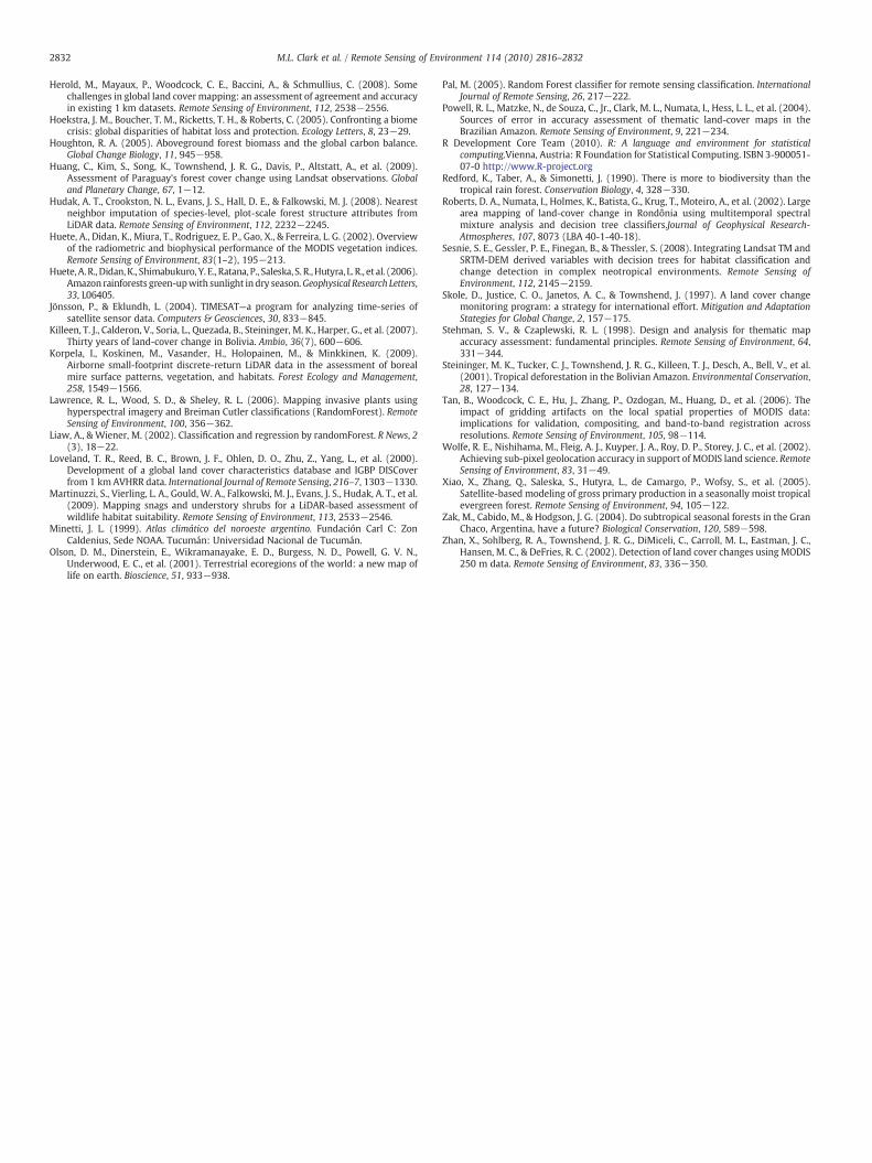
2832 M.L. Clark et al. / Remote Sensing of Environment 114 (2010) 2816–2832

Herold, M., Mayaux, P., Woodcock, C. E., Baccini, A., & Schmullius, C. (2008). Somechallenges in global land cover mapping: an assessment of agreement and accuracyin existing 1 km datasets. Remote Sensing of Environment, 112, 2538−2556.

Hoekstra, J. M., Boucher, T. M., Ricketts, T. H., & Roberts, C. (2005). Confronting a biomecrisis: global disparities of habitat loss and protection. Ecology Letters, 8, 23−29.

Houghton, R. A. (2005). Aboveground forest biomass and the global carbon balance.Global Change Biology, 11, 945−958.

Huang, C., Kim, S., Song, K., Townshend, J. R. G., Davis, P., Altstatt, A., et al. (2009).Assessment of Paraguay's forest cover change using Landsat observations. Globaland Planetary Change, 67, 1−12.

Hudak, A. T., Crookston, N. L., Evans, J. S., Hall, D. E., & Falkowski, M. J. (2008). Nearestneighbor imputation of species-level, plot-scale forest structure attributes fromLiDAR data. Remote Sensing of Environment, 112, 2232−2245.

Huete, A., Didan, K., Miura, T., Rodriguez, E. P., Gao, X., & Ferreira, L. G. (2002). Overviewof the radiometric and biophysical performance of the MODIS vegetation indices.Remote Sensing of Environment, 83(1–2), 195−213.

Huete,A.R., Didan,K., Shimabukuro, Y. E., Ratana, P., Saleska, S. R.,Hutyra, L. R., et al. (2006).Amazon rainforests green-upwith sunlight in dry season.Geophysical Research Letters,33, L06405.

Jönsson, P., & Eklundh, L. (2004). TIMESAT—a program for analyzing time-series ofsatellite sensor data. Computers & Geosciences, 30, 833−845.

Killeen, T. J., Calderon, V., Soria, L., Quezada, B., Steininger, M. K., Harper, G., et al. (2007).Thirty years of land-cover change in Bolivia. Ambio, 36(7), 600−606.

Korpela, I., Koskinen, M., Vasander, H., Holopainen, M., & Minkkinen, K. (2009).Airborne small-footprint discrete-return LiDAR data in the assessment of borealmire surface patterns, vegetation, and habitats. Forest Ecology and Management,258, 1549−1566.

Lawrence, R. L., Wood, S. D., & Sheley, R. L. (2006). Mapping invasive plants usinghyperspectral imagery and Breiman Cutler classifications (RandomForest). RemoteSensing of Environment, 100, 356−362.

Liaw, A., & Wiener, M. (2002). Classification and regression by randomForest. R News, 2(3), 18−22.

Loveland, T. R., Reed, B. C., Brown, J. F., Ohlen, D. O., Zhu, Z., Yang, L., et al. (2000).Development of a global land cover characteristics database and IGBP DISCoverfrom 1 km AVHRR data. International Journal of Remote Sensing, 216–7, 1303−1330.

Martinuzzi, S., Vierling, L. A., Gould, W. A., Falkowski, M. J., Evans, J. S., Hudak, A. T., et al.(2009). Mapping snags and understory shrubs for a LiDAR-based assessment ofwildlife habitat suitability. Remote Sensing of Environment, 113, 2533−2546.

Minetti, J. L. (1999). Atlas climático del noroeste argentino. Fundación Carl C: ZonCaldenius, Sede NOAA. Tucumán: Universidad Nacional de Tucumán.

Olson, D. M., Dinerstein, E., Wikramanayake, E. D., Burgess, N. D., Powell, G. V. N.,Underwood, E. C., et al. (2001). Terrestrial ecoregions of the world: a new map oflife on earth. Bioscience, 51, 933−938.

Pal, M. (2005). Random Forest classifier for remote sensing classification. InternationalJournal of Remote Sensing, 26, 217−222.

Powell, R. L., Matzke, N., de Souza, C., Jr., Clark, M. L., Numata, I., Hess, L. L., et al. (2004).Sources of error in accuracy assessment of thematic land-cover maps in theBrazilian Amazon. Remote Sensing of Environment, 9, 221−234.

R Development Core Team (2010). R: A language and environment for statisticalcomputing.Vienna, Austria: R Foundation for Statistical Computing. ISBN 3-900051-07-0 http://www.R-project.org

Redford, K., Taber, A., & Simonetti, J. (1990). There is more to biodiversity than thetropical rain forest. Conservation Biology, 4, 328−330.

Roberts, D. A., Numata, I., Holmes, K., Batista, G., Krug, T., Moteiro, A., et al. (2002). Largearea mapping of land-cover change in Rondônia using multitemporal spectralmixture analysis and decision tree classifiers.Journal of Geophysical Research-Atmospheres, 107, 8073 (LBA 40-1-40-18).

Sesnie, S. E., Gessler, P. E., Finegan, B., & Thessler, S. (2008). Integrating Landsat TM andSRTM-DEM derived variables with decision trees for habitat classification andchange detection in complex neotropical environments. Remote Sensing ofEnvironment, 112, 2145−2159.

Skole, D., Justice, C. O., Janetos, A. C., & Townshend, J. (1997). A land cover changemonitoring program: a strategy for international effort. Mitigation and AdaptationStategies for Global Change, 2, 157−175.

Stehman, S. V., & Czaplewski, R. L. (1998). Design and analysis for thematic mapaccuracy assessment: fundamental principles. Remote Sensing of Environment, 64,331−344.

Steininger, M. K., Tucker, C. J., Townshend, J. R. G., Killeen, T. J., Desch, A., Bell, V., et al.(2001). Tropical deforestation in the Bolivian Amazon. Environmental Conservation,28, 127−134.

Tan, B., Woodcock, C. E., Hu, J., Zhang, P., Ozdogan, M., Huang, D., et al. (2006). Theimpact of gridding artifacts on the local spatial properties of MODIS data:implications for validation, compositing, and band-to-band registration acrossresolutions. Remote Sensing of Environment, 105, 98−114.

Wolfe, R. E., Nishihama, M., Fleig, A. J., Kuyper, J. A., Roy, D. P., Storey, J. C., et al. (2002).Achieving sub-pixel geolocation accuracy in support of MODIS land science. RemoteSensing of Environment, 83, 31−49.

Xiao, X., Zhang, Q., Saleska, S., Hutyra, L., de Camargo, P., Wofsy, S., et al. (2005).Satellite-based modeling of gross primary production in a seasonally moist tropicalevergreen forest. Remote Sensing of Environment, 94, 105−122.

Zak, M., Cabido, M., & Hodgson, J. G. (2004). Do subtropical seasonal forests in the GranChaco, Argentina, have a future? Biological Conservation, 120, 589−598.

Zhan, X., Sohlberg, R. A., Townshend, J. R. G., DiMiceli, C., Carroll, M. L., Eastman, J. C.,Hansen, M. C., & DeFries, R. C. (2002). Detection of land cover changes using MODIS250 m data. Remote Sensing of Environment, 83, 336−350.