Remittances and Financial Openness

Michel Beine Elisabetta Lodigiani Robert Vermeulen

CESIFO WORKING PAPER NO. 3090 CATEGORY 7: MONETARY POLICY AND INTERNATIONAL FINANCE

JUNE 2010 PRESENTED AT CESIFO AREA CONFERENCE ON MACRO, MONEY & INTERNATIONAL FINANCE, FEBRUARY 2010

An electronic version of the paper may be downloaded • from the SSRN website: www.SSRN.com • from the RePEc website: www.RePEc.org

• from the CESifo website: Twww.CESifo-group.org/wp T

CESifo Working Paper No. 3090

Remittances and Financial Openness

Abstract Remittances have greatly increased during recent years, becoming an important and reliable source of funds for many developing countries. Therefore, there is a strong incentive for receiving countries to attract more remittances, especially through formal channels that turn to be either less expensive or less risky. One way of doing so is to increase their financial openness, but this policy option might generate additional costs in terms of macroeconomic volatility. In this paper we investigate the link between remittance receipts and financial openness. We develop a small model and statistically test for the existence of such a relationship with a sample of 66 mostly developing countries from 1980-2005. Empirically we use a dynamic generalized ordered logit model to deal with the categorical nature of the financial openness policy. We apply a two-step method akin to two stage least squares to deal with the endogeneity of remittances and potential measurement errors. We find a strong positive statistical and economic effect of remittances on financial openness.

JEL-Code: E60, F24, F41, O10.

Keywords: remittances, financial openness, government policy.

Michel Beine

CREA / University of Luxembourg michel.beine@uni.lu

Elisabetta Lodigiani

CREA / University of Luxembourg elisabetta.lodigiani@uni.lu

Robert Vermeulen CREA / University of Luxembourg

robert.vermeulen@uni.lu June 2010 We would like to thank Michael Binder, Herbert Brucker, Alessandra Casarico, Yin-Wong Cheung, Paul de Grauwe, Frédéric Docquier, Giovanni Facchini, Marcel Fratzscher, Frank Heinemann, Kajal Lahiri, Concetta Mendolicchio, Joan Muysken, Gianni Toniolo, Jean-Pierre Urbain, Timo Wollmershauser, participants of the 3rd TOM conference in Hamburg, 3rd MIFN workshop in Luxembourg, macro-lunch seminar at IRES Louvain-la-Neuve, the internal seminar in Luxembourg, the seminar at IAB in Nurnberg, the APPAM conference in Maastricht and the CES-Ifo annual workshop in international macroeconomics in Munich for helpful comments. The authors gratefully acknowledge support by the Fonds National de Recherche Luxembourg under grant FNR/VIVRE/06/30/10. All errors remain ours.

1 Introduction

Official global remittances sent to developing countries have reached 300 billion

US dollar in 2008 and have become a significant source of income for many

of these developing countries. In fact, for quite a few countries remittance

receipts exceed 20% of GDP (e.g. Guyana, Honduras, Jordan and several more).

These remittances appear to be a stable source of income over time , compared

to e.g. foreign direct investment, and their value quite often exceeds official

development aid. The importance of remittances has been recognized by policy

makers, global institutions, such as the World Bank, and academics alike.1

A growing academic literature has been devoted to analyze the microeco-

nomic and macroeconomic effects of remittances in developing countries (see

Schiff and Ozden, 2006, 2007, for a synthesis). The effects of remittances on re-

ceiving countries seem indeed numerous. At a microeconomic level, remittances

have been found to boost investment in human capital and educational attain-

ments, thereby reducing poverty in many developing countries. Furthermore,

there is significant evidence that remittances increase not only consumption

but tend to also raise health levels and investment in public infrastructure. At

a macroeconomic level, the existence of a positive relationship between remit-

tances and growth is more controversial. While remittances tend to favor the

accumulation of important production factors such as physical capital and edu-

cation, they exert detrimental effects in terms of labor market incentives. They

also create ’Dutch disease’ effects through the appreciation of domestic curren-

cies, leading to further deindustrialization in the receiving country. Neverthe-

less, the recent literature shows that appropriately used migrant remittances,

combined with sound government policies, have a positive net effect on economic

growth.

The growing importance of remittances and their positive impact on the

economic conditions in receiving countries create for their governments strong

incentives to facilitate the attraction of those flows. In some countries such as

Mexico and the Philippines, explicit programs have been set up to increase the

flows of the received remittances. Among the possible schemes aimed at boosting

these receipts, the opening of financial borders is a possible policy instrument of

governments. By decreasing the cost of the remittances sent through the official

way or by relaxing the restriction of financial flows coming from abroad, govern-

ments can significantly boost the total amount of the received funds. Financial

openness creates, however, new costs and risks for the receiving countries. One

of the most important costs is the increased exposure to financial crises and to

1In particular, given the importance of the remittances for a large set of countries, theWorld Bank devoted substantial efforts to monitor, understand and forecast remittance flows.See website link www.go.worldnak.org/ssw3DDNL.

2

macroeconomic instability. Therefore, the final decision to open the financial

borders is likely to result from a trade-off between the various benefits drawn

from the attracted remittances and the increased macroeconomic risk. In turn,

those benefits will depend on the initial size of the incoming remittances, which

depend on a set of factors unrelated to financial openness. Those factors include

among others the size of the existing diaspora and their location.

In this paper, we proceed to a political economy investigation of the choice

of the degree of financial openness by government with respect to their situation

in terms of incoming remittances. We first develop a small model that expresses

the trade off faced by government in their decision to open the financial borders.

We show that the optimal degree of openness depends on the initial size of the

incoming remittances which in turn depends on factors that are exogenous for

the government, such as the size the total diaspora, its location or the economic

conditions of the destination countries. Then, we investigate empirically that

link for a sample of 66 mostly developing countries from 1980-2005. Financial

openness is classified according to three regimes (closed, neutral or open) based

on the KAOPEN financial openness indicator of Chinn and Ito (2008). In

addition to remittances we account for institutional quality, trade openness and

domestic financial development.

Empirically we use a dynamic generalized ordered logit model to establish the

link between remittances and financial openness. This framework is attractive

because it is well suited to deal with the ordinal nature of the financial openness

indicator. Moreover, it is possible to take unobserved heterogeneity into account.

In addition, we apply a two-step method akin to two stage least squares to deal

with the endogeneity of remittance receipts and potential measurement errors.

To preview our results, we find a strong positive effect of remittances on

financial openness. The more remittances a country receives, the more likely it

will be financially open. The positive effect of remittances on financial openness

is robust to instrumentation of remittances, both in a balanced and unbalanced

sample.

A counterfactual analysis shows that remittances have an important effect

on country’s financial openness policy. Results indicate that large remittance

receiving countries have a much larger probability of being financially closed

when they do not receive remittances anymore.

The paper is organized as follows. We first review the existing related liter-

ature and provide some stylized facts(Section 2). In Section 3 we introduce a

theoretical model that captures the trade-off between the benefits and the costs

of opening the financial borders and hence the determinants of the government’s

decision. The empirical model and results are discussed in Section 4. In Section

5 we study two counterfactual scenarios to assess the economic importance of

3

remittance receipts for individual countries. Section 6 concludes.

2 Motivation, existing related literature and styl-

ized facts

In this section, we cover the related literature. Our paper provides a political

economy analysis of the choice of financial openness based on the incentive to

attract remittances from abroad. It is thus related to the literature on the effects

of remittances and the one dealing with financial integration. We also provide

specific examples of governmental schemes. Finally, we provide preliminary

evidence in favour of a link between the cost to remit and the degree of financial

openness of the receiving country.

2.1 Related literature on the effects of remittances

The exiting literature on the impact of remittances suggests that remittances

exert important effects on the economic situation of the receiving countries.

The academic debate has focused on both micro- and macroeconomic ef-

fects of remittances. First, a number of micro studies investigate the poverty

reduction effect of remittances. Country studies show that remittances play an

important role in reducing poverty in e.g. Lesotho (Gustafsson and Makonnen,

1993), Guatemala (Adams, 2006) and Mexico (Acosta et al., 2006). A second

strand investigates how remittance recipients spend their receipts. In general,

households either consume or invest their receipts, where investment (especially

in human capital) can potentially accelerate future economic growth. Recent

studies (e.g. Dustmann and Kirchkamp, 2002; Cox-Edwards and Ureta, 2003;

Adams, 2006) show that a sizable fraction of remittances are invested in edu-

cation, health care and physical assets. Indeed, beyond the direct effect that

remittances exert on spending, the fact that households receive money from

abroad can be seen as a strong increase in collateral that in turn might increase

investment. Remittances alleviate liquidity constraints that can act as impor-

tant constrains on investment in education in a set of developing countries. In

countries with a minimal level of banking development, the permanent inflow of

remittances can act as a collateral for borrowing by the households. In turn, this

might favour investment in human capital, small businesses or infrastructure.

Finally, since remittances give rise to some increase in aggregate consumption,

this leads to increase in public revenues in countries that tax consumption.

In response, macroeconomic studies started to focus on the effects of remit-

tances on economic growth. While there is ample evidence that remittances

4

reduce poverty (Adams and Page, 2005) and boost aggregate demand, the ef-

fects on growth are not clear cut. One reason is that remittances might alter the

behaviour of receiving households (the so-called moral hazard effects) or induce

price developments that are detrimental for the development of the country.

One of these effect is the so-called Dutch Disease effect through which the flow

of remittances induces a real exchange rate appreciation that affects negatively

the activity of the tradable manufacturing sector (Acosta et al., 2009).

However, recent studies find that remittances have a positive impact on eco-

nomic growth. Giuliano and Ruiz-Arranz (2008) show that in the economies

where the financial system is underdeveloped, remittances alleviate credit con-

straints and work as a substitute for financial development, improving the al-

location of capital and therefore accelerating economic growth. On the other

hand, Mundaca (2009) shows that financial development potentially leads to

better use of remittances, thus fostering growth. Recent research conducted by

Aggarwal et al. (2006) also shows that remittances may directly promote finan-

cial development. In particular, they find that remittances have a significant

and positive impact on bank deposits to GDP. Overall, the literature finds that

net effect on growth seems to be positive, without even considering the positive

impact remittances can have on the income distribution.

2.2 Government policies

The favourable effects of remittances on the economic situation of receiving

countries have induced some governments to implement specific programs to

promote remittance receipts.

The Philippines provides a clear-cut example, where the government ex-

plicitly promotes emigration to receive remittances. In 1982, the Philippine

Overseas Employment Administration (POEA) has been created by Executive

Order No. 797. Article I of this order clearly mentions the main objectives:

∙ “3. Recruitment and place workers to service the requirements of overseas

employers for trained and competent Filipino workers;”

∙ “4. Promote the development of skills and careful selection of Filipino

workers for overseas employment;”

∙ “7. Generate Foreign exchange from the earnings of Filipinos employed

under its programs;”

These objectives clearly show that the Philippine government’s aim is to

maximize remittance receipts. Moreover, articles VII and IX state the objectives

even clearer:

5

∙ “k. Formulate and implement programs for the effective monitoring of

foreign exchange remittances of overseas contract workers.” (Art. VII,

Sec. 31)

∙ “4. Maximize foreign exchange generation from Filipino workers and sea-

men;” (Art. IX, Sec. 37)

The Mexican program Citizen Initiative 3x1 (Iniciativa Ciudadana 3x1 in

Spanish) is another example of a government initiated scheme to promote re-

mittance receipts from migrants. In the United States Mexican migrants run

over 2000 so called Hometown Associations (HTAs), which support their local

communities in Mexico. Under Citizen Initiative 3x1 remittances from Mexican

HTAs are matched with local, state and federal governments’ funds to finance

mostly basic infrastructure in rural areas. By investing in basic infrastructure,

such as building roads, bridges and irrigation systems, necessary conditions are

created for economic growth. In effect, remittances are generous and in some

municipalities the funds received by Citizen Initiative 3x1 are larger than the

municipality’s total budget (Orozco and Lapointe, 2004).

By matching migrant’s remittances the Mexican government is able to chan-

nel remittance receipts to productive use, which benefits the country’s long term

growth. In addition, the development of rural areas reduces the problems in-

duced by urbanization, e.g. lack of proper housing for Mexico City’s expanding

population. The success of the program is enormous and the only problem the

government faces is that

“[t]he amounts committed to the program by HTAs has increased so rapidly

in recent years that, at times, the government does not have the budget to match

the funds” (Maimbo and Ratha, 2005, p. 123).

While some specific microeconomic programs such as those presented above

might be desirable, there are complementary macroeconomic reforms that can

be implemented on a larger scale.2 One example is the choice of the exchange

rate regime. Freund and Spatafora (2008) find that the existence of multiple

exchange rates significantly reduces the amount of recorded remittances. Singer

(2009) shows that the size of incoming remittances increase the likelihood that

policymakers of developing countries will adopt fixed exchange rates. Our paper

considers an alternative policy option , i.e. the openness of the financial borders.

Financial liberalization turns out to be a more global option encompassing the

choice of the exchange rate regime.3

2For several other examples of government programs to promote remittance receipts seee.g. Maimbo and Ratha (2005).

3Our indicator of financial openness includes the existence of multiple exchange rates forinstance.

6

Financial liberalization exerts two specific effects on the flows of remittances.

First, financial liberalization facilitates foreign financial transactions. In case of

financial autarky, it is almost impossible for some migrants to send remittances

through the formal way. While informal ways can always be relied on and

are not always more expensive at first glance, these involve much more risk.

Furthermore, the informal channel is often used for illegal purposes, with the

danger of being considered as a criminal.4 For some pairs of countries that are

quite distant, physical transportation of money might be not only dangerous

but also may involve higher costs. Second, more financial openness will also

lower (formal) remittances’ transaction costs and will provide incentives to send

remittances trough the formal market. Financial borders are often associated

to controls and constraints on international financial flows such as foreign direct

investments, portfolio investments and remittances sent through the banking

system. This leads to an increase in the cost and to lower transfers compared

to a liberalized regime.

2.3 Stylized facts

To illustrate the impact of financial openness on the cost of sending remittances,

Table 1 provides the results of a gravity regression relating the (bilateral) cost

of sending remittances from country i to country j and the degree of financial

openness in country j. The cost of sending remittances denoted by cij is drawn

from the new dataset built by the World Bank on the remittance costs across

134 country corridors, involving 14 sending countries and 72 potential receiving

countries. The data come from a survey conducted by the World Bank and are

available only for 2008 and 2009.5

The World bank data include two components of the cost of remitting, i.e.

the exchange rate margin associated to currency conversion and the fixed fee

associated to the international transfer. The data reveals that the total cost

of remitting can be substantial. Total costs of more than 15 percent are not

unusual. Furthermore, those costs are observed for the most popular transfer

corridors. They might be expected to be even more important for remitting

between less popular country pairs. We report here the regression results ob-

tained with the cost of sending 500 USD but we get quite the same qualitative

conclusions with the other measure based on the cost of sending 200 USD.

In line with Beck and Peria (2009), we account for factors that are bilat-

eral to i and j, origin specific and destination specific. Since our purpose is

4See for instance http://www.interpol.int/Public/FinancialCrime/MoneyLaundering/Hawala/default.asp about the Hawala system, one of the most popular informal channelsfor remittances, and money laundering.

5The full data and the related explanations are available at www.remittanceprices.org.

7

to focus on the impact on destination specific factors such as financial open-

ness and since our dataset is only cross-sectional, we capture the origin specific

factors by fixed effects, denoted by �i. Included bilateral factors are the log

of distance between the two countries, the log of the stock of migrants from

country j living in country i, the existence of colonial links and a common

official language. For convenience in exposition, these factors are collected in

the matrix xij,k in Equation (1). The destination specific factors include some

index of bank concentration (Herfindahl index) to capture the impact of bank

competition (denoted by bankj) and our index of financial integration (denoted

by kaopenj). The index of financial integration we use in this paper is the

KAOPEN index developed by Chinn and Ito (2008). We provide more informa-

tion on this indicator in Section 4.1. The higher the index, the more financially

open a country is.

The estimated equation is:

cij = �i + �1kaopenj + �2bankj +∑k

kxij,k + �ij (1)

The results in Table 1 shed light on the relationship between financial open-

ness and the cost of sending remittances through the official channel. In both

specifications reported in Table 1, �1 is found to be negative and significant

at the 5 percent level. The results show that the higher the openness of the

receiving countries, the lower the cost to send remittances to that country,

everything equal elsewhere. The results suggest that one reason to open the

financial borders for governments of remittances receiving countries is to lower

the transaction costs. In turn, this should increase the total amount sent by the

migrants, especially since the cost is supported by them.

Table 1: Cost of remitting $ 500

variable (1) (2)kaopen -0.256** -0.270**

(0.126) (0.125)bank concentration host 4.347*** 3.991***

(0.919) (0.842)log(number of migrants) -0.246 -0.277**

(0.158) (0.124)common language -0.385

(0.481)distance 0.000

(0.000)colony 0.153

(0.564)Observations 89 89R2 0.956 0.955

Note: Estimation of Equation (1) using OLS, withrobust standard errors. *,**,*** imply significanceat the 10%, 5% and 1%, respectively.

8

The World Bank dataset also reveals an important feature concerning the

operating country corridors. The dataset covers 14 sending countries and 72

receiving countries. Nevertheless, prices were obtained by the surveyors of the

WB only for 134 country corridors. This means that the dataset contains 87

percent of missing observations. Of course, the reasons of those missing obser-

vations might be numerous. Part of the missing data might be due to the fact

that it is possible to send remittances but that the cost was unknown by the

service providers at the time of the survey. In turn, the prices might be unknown

because there is little demand for that particular corridor. Importantly, some

missing data might also reflect that some or all service providers do not offer

that service for this particular country corridor. Whatever the various reasons,

the important proportion of missing data for the costs of sending remittances

suggests that in many case, sending remittances through the formal channel

might be cumbersome for the migrants. Part of the impossibility of sending

remittances to a particular country might be due to the fact that the country

is not fully opened to international financial flows.

2.4 Financial openness as an option

A related literature in international finance investigates the relationship be-

tween capital account/financial openness, financial development and economic

growth.6 A large number of studies find a positive effect of financial openness

on economic growth (e.g. Quinn, 1997; Bekaert et al., 2005; Quinn and Toyoda,

2008). However, this positive view is challenged by others (e.g. Edison et al.,

2002). Klein and Olivei (2008) argue that the lack of a positive growth effect

of financial openness in developing countries is due to a missing effect of finan-

cial openness on financial development for these countries. However, Chinn and

Ito (2006) do find a positive effect of financial openness on domestic financial

development if the institutional quality in the country is of a sufficiently high

level.

The importance of threshold levels of institutional quality and macroeco-

nomic policies has been advocated further by Kose et al. (2009). Due to the

positive effects of remittances on macroeconomic stability and financial develop-

ment, it is attractive for remittance receiving countries to liberalize their capital

account and increase their financial openness to accelerate economic growth.

Hence, remittances can have an important direct effect on a developing coun-

tries’ financial openness and therefore an indirect impact on growth. However,

6Remittances are recorded in both the current and capital account of the balance of pay-ments. Hence, when we refer to capital account/financial openness this ought to be interpretednot strictly as capital account transactions. Therefore, we use the more general term financialopenness to assess the ease of sending and receiving remittances.

9

financial openness does not only have positive effects, but also creates costs for

governments. First, from the Mundell-Fleming model we know that the govern-

ment needs to give up either exchange rate stability or monetary policy when

allowing the free movement of capital. If the government aims to control all

three factors, countries risk being hit by speculative attacks, where the only op-

tion left is to devaluate the currency. The Argentine experience during the early

2000s is an illustrative example. In order to curtail inflation in the early 1990s

Argentina pegged its currency to the US$. Due to large public deficits (financed

in part by the Central Bank) and a revaluation of the US$ vs. the Brazilian

real and the euro made Argentina’s export sector uncompetitive. Hence, both

imports and foreign debt increased. This resulted in a severe economic crisis

and in 2002 the peg with the US$ was abandoned.

Second, financial openness induces potential contagion effects, where healthy

countries can become affected due to ill neighbors. Kaminsky and Reinhart

(2000) show the important role of the financial sector and how the actions

of financial market participants can lead to instability, facilitated by financial

openness. This contagion risk was especially prevailing during the 1997 Asian

financial crisis, where countries such as Korea had sound macroeconomic poli-

cies, but entered in economic hardship due to capital flight induced by herd

behavior. In addition, financial openness increases the comovement of stock

markets, especially in times of crisis (Beine et al., 2010). Hence, countries will

become more integrated in the world economy and be less able to steer their own

economy. The potential positive and negative effects of financial openness need

to be weighted by governments in their choice regarding the degree of financial

openness. More specifically for developing countries, they need to weight the

positive effects of remittances to the potential risks of increased macroeconomic

volatility.

3 The Model

This section formalizes the trade off a remittance receiving country’s govern-

ment faces: the positive economic effects of remittance receipts vs. potentially

increasing macroeconomic instability. To keep the model tractable and intuitive,

we consider a simple static model with 3 decision agents: one migrant remitter

(m), one recipient household (f), which can consist of one or more individuals,

and the government of the receiving household’s country whose objective it is

to maximize revenues.7

7In this section we want to introduce a very simple and intuitive model to provide insightsin the underlying mechanisms of the government’s financial openness policy. We decide to usea static model for illustrative purposes since a dynamic model will be much more complex,being beyond the scope of this section. The empirical model we are going to test includes

10

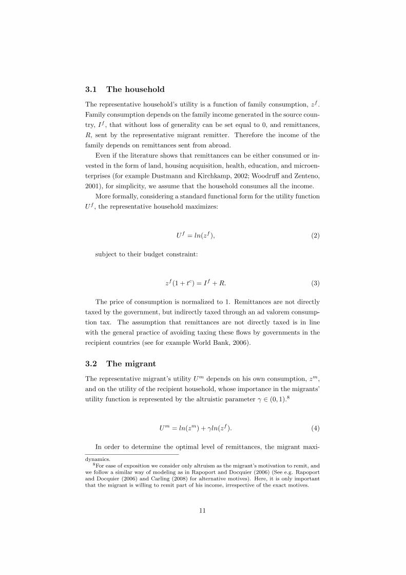
3.1 The household

The representative household’s utility is a function of family consumption, zf .

Family consumption depends on the family income generated in the source coun-

try, If , that without loss of generality can be set equal to 0, and remittances,

R, sent by the representative migrant remitter. Therefore the income of the

family depends on remittances sent from abroad.

Even if the literature shows that remittances can be either consumed or in-

vested in the form of land, housing acquisition, health, education, and microen-

terprises (for example Dustmann and Kirchkamp, 2002; Woodruff and Zenteno,

2001), for simplicity, we assume that the household consumes all the income.

More formally, considering a standard functional form for the utility function

Uf , the representative household maximizes:

Uf = ln(zf ), (2)

subject to their budget constraint:

zf (1 + tc) = If +R. (3)

The price of consumption is normalized to 1. Remittances are not directly

taxed by the government, but indirectly taxed through an ad valorem consump-

tion tax. The assumption that remittances are not directly taxed is in line

with the general practice of avoiding taxing these flows by governments in the

recipient countries (see for example World Bank, 2006).

3.2 The migrant

The representative migrant’s utility Um depends on his own consumption, zm,

and on the utility of the recipient household, whose importance in the migrants’

utility function is represented by the altruistic parameter ∈ (0, 1).8

Um = ln(zm) + ln(zf ). (4)

In order to determine the optimal level of remittances, the migrant maxi-

dynamics.8For ease of exposition we consider only altruism as the migrant’s motivation to remit, and

we follow a similar way of modeling as in Rapoport and Docquier (2006) (See e.g. Rapoportand Docquier (2006) and Carling (2008) for alternative motives). Here, it is only importantthat the migrant is willing to remit part of his income, irrespective of the exact motives.

11

mizes his utility function subject to his budget constraint, given by:

zm = Im −R(1 + �), (5)

where zm denotes consumption of the migrant, Im and R denote respec-

tively the income of the migrant and the amount of remittances. The price of

consumption, as before, is normalized to 1, therefore, prices are assumed to be

the same across the host and origin country. However, this assumption does not

change any of the substantive implications of the model. The cost of sending re-

mittances depends on the parameter �, a kind of iceberg cost, which reflects the

degree of financial openness of the migrant origin country. The more open the

country is, the less costly is to send remittances home and vice versa. Costs can

be interpreted in a broader sense, i.e. in terms of easiness of the transactions.9

Ruling out the possibility of negative transfers from the migrant to the house-

hold, the maximization problem of the migrant can be written as:

maxR

Um = ln(Im −R(1 + �)) + ln((If +R)/(1 + t))

= ln(Im −R(1 + �)) + ln(If +R)− ln(1 + t). (6)

The first order condition is given by:

∂Um/∂R = − 1 + �

Im −R(1 + �)+

If +R= 0, (7)

and the optimal amount of remittances is

R∗ = Im

(1 + �)(1 + )− If

1 + . (8)

Doing some comparative-statics, it is easy to see that the model predicts that

transfers to the origin household increase with the income of the migrant, ∂R∂Im >

0, and with the altruistic parameter, ∂R∂ > 0, and decrease with the wealth of

the origin family, ∂R∂If

< 0. Moreover, transfers are decreasing in �, ∂R∂� < 0,

predicting that the more the home country is financially closed, the less migrants

are going to remit.

9The cost can be interpreted also as the “risks in sending remittances”. It is plausibleto think that a more open financial system provides incentives to use the formal systemin sending remittances, therefore lowering the risks faced when sending money through theinformal channel. A lower risk will induce more remittances. Here, we do not distinguishbetween formal and informal remittances, as only the formal ones are observed.

12

3.3 The government

The government chooses the degree of financial openness in order to maximize its

revenues, which it derives from taxing consumption. Since remittances are fully

spend on consumption, the government tries to maximize remittances receipts.

Hence, the government has a strong incentive to open its financial borders to

attract remittances. On the other hand, controls are beneficial, because they

insulate domestic markets from external shocks. Ceteris paribus, the more open

a country is, the higher is capital flow volatility, the probability of external

shocks and economic crises.10 Naturally, the risk of incurring a financial crisis

depends on several country characteristics, e.g. institutional quality.

We introduce a simple cost function to capture the risk-cost of the govern-

ment. The government incurs a country-specific cost �, which it will pay with

probability � ∈ [0, 1]. We assume that the probability is decreasing in �, and

it is equal to 0 when � → +∞ (fully closed) and equal to 1 when � = 0 (fully

open).

More formally, the government maximization problem is given by

max�

Vg = zf t− ��

=t

(1 + t)(If +R)− ��, (9)

The first order condition is

∂V/∂� =t

(1 + t)

∂R

∂�− � ∂�

∂�= 0. (10)

From Equation (8) it is easy to see that ∂R∂� < 0, predicting that the more

financially closed the home country is, the less migrants are going to remit.

At the same time ∂�∂� is negative, meaning that the more the home country is

financially closed, the lower the probability to pay a cost �. In order to determine

the optimum level of �, the government faces the trade-off between the expected

earnings that it will derive from the (indirect) taxation of remittances and the

expected cost of opening, cost depending on country characteristics.

For given t, then the optimum � will depend negatively on R and positively

on �, �∗ = �(R, �). In case of interior solution, the government may choose a �∗

which reflects intermediate or limited openness.

More explicitly, for analytical tractability, let’s take the particular case for

10Alesina et al. (1994) list four main motives for capital controls: (i) limit volatile capitalflows; (ii) maintain the domestic tax base; (iii) retain domestic savings; and (iv) sustainstructural reform. Even if Alesina et al. (1994) identify the governments’ attempt to collectrevenue from financial repression as the main motive for controls, there are a lot of exampleswhere financial crises were mainly due to capital flights (for example the Asian crisis in 1997).

13

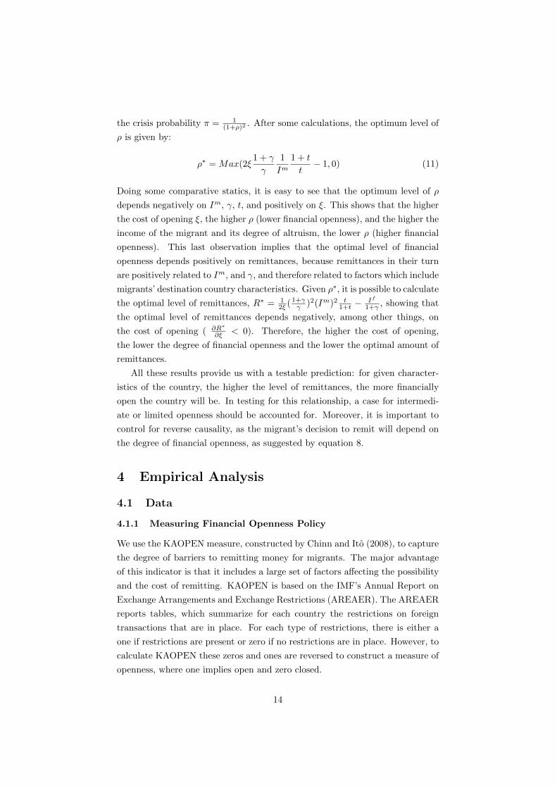
the crisis probability � = 1(1+�)2 . After some calculations, the optimum level of

� is given by:

�∗ = Max(2�1 +

1

Im1 + t

t− 1, 0) (11)

Doing some comparative statics, it is easy to see that the optimum level of �

depends negatively on Im, , t, and positively on �. This shows that the higher

the cost of opening �, the higher � (lower financial openness), and the higher the

income of the migrant and its degree of altruism, the lower � (higher financial

openness). This last observation implies that the optimal level of financial

openness depends positively on remittances, because remittances in their turn

are positively related to Im, and , and therefore related to factors which include

migrants’ destination country characteristics. Given �∗, it is possible to calculate

the optimal level of remittances, R∗ = 12� ( 1+

)2(Im)2 t1+t −

If

1+ , showing that

the optimal level of remittances depends negatively, among other things, on

the cost of opening ( ∂R∗

∂� < 0). Therefore, the higher the cost of opening,

the lower the degree of financial openness and the lower the optimal amount of

remittances.

All these results provide us with a testable prediction: for given character-

istics of the country, the higher the level of remittances, the more financially

open the country will be. In testing for this relationship, a case for intermedi-

ate or limited openness should be accounted for. Moreover, it is important to

control for reverse causality, as the migrant’s decision to remit will depend on

the degree of financial openness, as suggested by equation 8.

4 Empirical Analysis

4.1 Data

4.1.1 Measuring Financial Openness Policy

We use the KAOPEN measure, constructed by Chinn and Ito (2008), to capture

the degree of barriers to remitting money for migrants. The major advantage

of this indicator is that it includes a large set of factors affecting the possibility

and the cost of remitting. KAOPEN is based on the IMF’s Annual Report on

Exchange Arrangements and Exchange Restrictions (AREAER). The AREAER

reports tables, which summarize for each country the restrictions on foreign

transactions that are in place. For each type of restrictions, there is either a

one if restrictions are present or zero if no restrictions are in place. However, to

calculate KAOPEN these zeros and ones are reversed to construct a measure of

openness, where one implies open and zero closed.

14

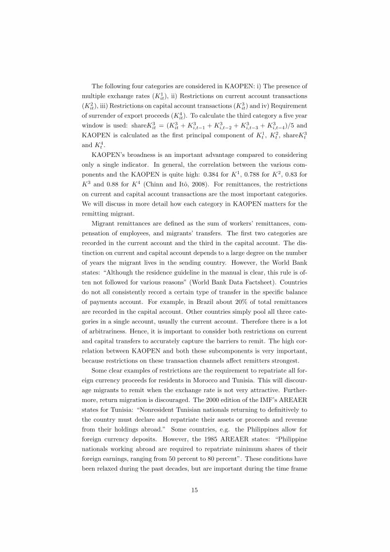
The following four categories are considered in KAOPEN: i) The presence of

multiple exchange rates (K1it), ii) Restrictions on current account transactions

(K2it), iii) Restrictions on capital account transactions (K3

it) and iv) Requirement

of surrender of export proceeds (K4it). To calculate the third category a five year

window is used: shareK3it = (K3

it + K3i,t−1 + K3

i,t−2 + K3i,t−3 + K3

i,t−4)/5 and

KAOPEN is calculated as the first principal component of K1t , K2

t , shareK3t

and K4t .

KAOPEN’s broadness is an important advantage compared to considering

only a single indicator. In general, the correlation between the various com-

ponents and the KAOPEN is quite high: 0.384 for K1, 0.788 for K2, 0.83 for

K3 and 0.88 for K4 (Chinn and Ito, 2008). For remittances, the restrictions

on current and capital account transactions are the most important categories.

We will discuss in more detail how each category in KAOPEN matters for the

remitting migrant.

Migrant remittances are defined as the sum of workers’ remittances, com-

pensation of employees, and migrants’ transfers. The first two categories are

recorded in the current account and the third in the capital account. The dis-

tinction on current and capital account depends to a large degree on the number

of years the migrant lives in the sending country. However, the World Bank

states: “Although the residence guideline in the manual is clear, this rule is of-

ten not followed for various reasons” (World Bank Data Factsheet). Countries

do not all consistently record a certain type of transfer in the specific balance

of payments account. For example, in Brazil about 20% of total remittances

are recorded in the capital account. Other countries simply pool all three cate-

gories in a single account, usually the current account. Therefore there is a lot

of arbitrariness. Hence, it is important to consider both restrictions on current

and capital transfers to accurately capture the barriers to remit. The high cor-

relation between KAOPEN and both these subcomponents is very important,

because restrictions on these transaction channels affect remitters strongest.

Some clear examples of restrictions are the requirement to repatriate all for-

eign currency proceeds for residents in Morocco and Tunisia. This will discour-

age migrants to remit when the exchange rate is not very attractive. Further-

more, return migration is discouraged. The 2000 edition of the IMF’s AREAER

states for Tunisia: “Nonresident Tunisian nationals returning to definitively to

the country must declare and repatriate their assets or proceeds and revenue

from their holdings abroad.” Some countries, e.g. the Philippines allow for

foreign currency deposits. However, the 1985 AREAER states: “Philippine

nationals working abroad are required to repatriate minimum shares of their

foreign earnings, ranging from 50 percent to 80 percent”. These conditions have

been relaxed during the past decades, but are important during the time frame

15

we study.

Other examples include Vietnam, which mandates migrants to invest 30

percent of their remittances in a government fund. Some countries, such as

Colombia and Ecuador tax remittances, whereas others, e.g. Brazil, mandate

that all foreign exchange go through the central bank (Agunias, 2006). However,

during the eighties and nineties more countries imposed restrictions, but many

of these were abandoned once the governments realized the positive effects of

remittances. The AREAER indicates that quite a few countries require the

surrender of export proceeds. This requirement is also closely related to the

mandatory conversion of foreign currencies into domestic currency. While not

affecting directly migrants, the requirement of surrender of export proceeds

might be considered as reflecting some uncertainty regarding the extortion of

remittances. Hence, including this factor in KAOPEN helps to obtain a more

complete picture of the total financial openness policy of a country.

The existence of multiple exchange rates creates extra costs for migrants

remitting. In fact, Freund and Spatafora (2008) show that the existence of mul-

tiple exchange rates significantly reduces the amount of recorded remittances.

In addition, the World Bank data on the cost of remitting shows that there are

sizeable exchange rate margins (extra costs above interbank rate) for several

countries when remitting internationally. For example, when transferring from

the U.S. to Brazil the average exchange rate margin is around 3%, from the

U.K. to Kenya 5%, from France to Morocco 2%, Canada to India 5%, etcetera.

There is quite some competition in these remittance corridors, so costs will be

even higher for less popular country pairs. Those exchange rate margins are of

course added to the fixed fee associated to the transfer.

Dual exchange rates are still in place for a large number of countries (Rein-

hart and Rogoff, 2004). As remitters are most likely low priority, they will not

receive the most favorable exchange rate, which makes remitting less attractive.

However, countries receiving large amounts of remittances are more likely to

opt for a fixed exchange rate regime (Singer, 2009). Naturally, fixed exchange

rates reduce the costs of remitting. Hence, we expect large remittance receiving

countries to have a very low probability of a double exchange rate regime.

Quite often a dual exchange rate regime is in place after a balance of pay-

ments crisis. For example, India opted for a dual exchange rate regime in 1992

right after the balance of payments crisis of 1991. Basically, there was an official

rate for selected government and private transactions and a market determined

rate for all other transactions. Naturally, this market rate was worse than the

official rate.

To sum up, the KAOPEN index is a broad indicator of financial openness,

which captures a set of various relevant factors affecting the cost of remitting.

16

It is therefore more representative of the overall policy of a country regarding

its degree of financial openness. As we are interested in government policy mea-

sures, de facto indicators of financial openness policy based on parity conditions

or cross border asset holdings are of limited use to address this paper’s research

question.

Due to its straightforward and transparent construction KAOPEN is avail-

able for virtually all countries in the world. The indicator is easily constructed

and therefore annually updated.11 This large coverage is necessary to analyze

the large number of countries in this study. In this paper a subset of 66 coun-

tries is considered. This restricted set of 66 countries is due to the exclusion of

OECD countries and the requirement of full data availability for KAOPEN and

remittances data from 1980 until 2005. Alternative financial openness policy

indicators by Quinn (1997) and Miniane (2004) do not cover a large enough

country span and do not fully cover the timeframe we consider.12 For the com-

mon country/timeframe KAOPEN shows a strong correlation with the other

two indicators.

Figure 1 shows a quantile graph of the KAOPEN database pooling all 66

countries across all years. The values of KAOPEN range between about -1.9

and 2.6. Note that these values are not of a cardinal nature, i.e. -1 is not twice

as closed as -0.5. The higher KAOPEN the more financially open a country is.

Figure 1: Quantile graph of KAOPEN 1980-2005

11The data and a detailed description on its construction are available athttp://www.ssc.wisc.edu/∼mchinn/research.html. Recently, an updated version of thedatabase up to 2007 has been released.

12For a detailed comparison of different indicators we refer to Edison et al. (2004) andMiniane (2004).

17

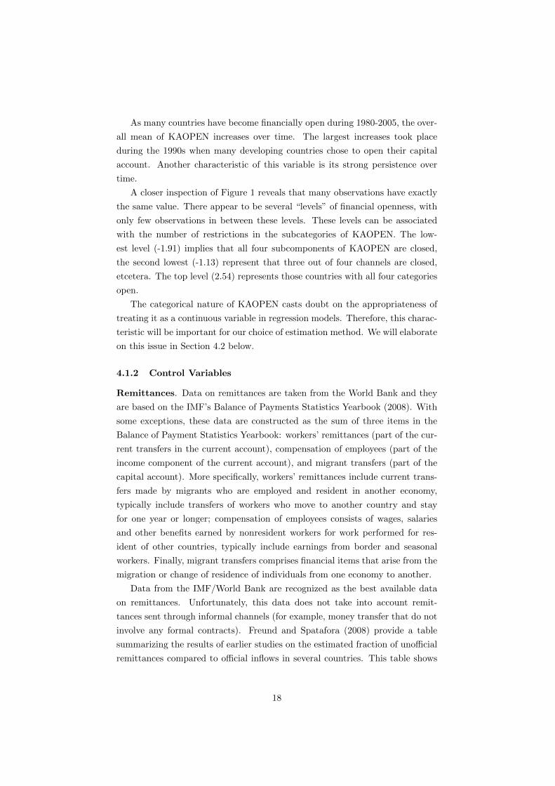
As many countries have become financially open during 1980-2005, the over-

all mean of KAOPEN increases over time. The largest increases took place

during the 1990s when many developing countries chose to open their capital

account. Another characteristic of this variable is its strong persistence over

time.

A closer inspection of Figure 1 reveals that many observations have exactly

the same value. There appear to be several “levels” of financial openness, with

only few observations in between these levels. These levels can be associated

with the number of restrictions in the subcategories of KAOPEN. The low-

est level (-1.91) implies that all four subcomponents of KAOPEN are closed,

the second lowest (-1.13) represent that three out of four channels are closed,

etcetera. The top level (2.54) represents those countries with all four categories

open.

The categorical nature of KAOPEN casts doubt on the appropriateness of

treating it as a continuous variable in regression models. Therefore, this charac-

teristic will be important for our choice of estimation method. We will elaborate

on this issue in Section 4.2 below.

4.1.2 Control Variables

Remittances. Data on remittances are taken from the World Bank and they

are based on the IMF’s Balance of Payments Statistics Yearbook (2008). With

some exceptions, these data are constructed as the sum of three items in the

Balance of Payment Statistics Yearbook: workers’ remittances (part of the cur-

rent transfers in the current account), compensation of employees (part of the

income component of the current account), and migrant transfers (part of the

capital account). More specifically, workers’ remittances include current trans-

fers made by migrants who are employed and resident in another economy,

typically include transfers of workers who move to another country and stay

for one year or longer; compensation of employees consists of wages, salaries

and other benefits earned by nonresident workers for work performed for res-

ident of other countries, typically include earnings from border and seasonal

workers. Finally, migrant transfers comprises financial items that arise from the

migration or change of residence of individuals from one economy to another.

Data from the IMF/World Bank are recognized as the best available data

on remittances. Unfortunately, this data does not take into account remit-

tances sent through informal channels (for example, money transfer that do not

involve any formal contracts). Freund and Spatafora (2008) provide a table

summarizing the results of earlier studies on the estimated fraction of unofficial

remittances compared to official inflows in several countries. This table shows

18

that are quite a few differences between countries and that the share of unofficial

remittances may be quite high in some cases. For example, the share of infor-

mal remittances is quite low in Guatemala and the Dominican Republic, 5%

and 15% respectively. However, in other countries the majority of remittances

received may be unofficial, e.g. Bangladesh 54% and Uganda 80%.13

Other data. In order to explain the determinants of financial openness,

data drawn from a several number of sources are considered.

Financial development measures. Measures of financial development are ex-

tracted from the data set of Beck et al. (2000). In particular we consider the

ratio of bank credit over bank deposit and a measure of liquid liabilities over

GDP.

Institutional quality measures. In order to consider the importance of in-

stitutional quality on the degree of financial openness, we use the composite

Polity2 index from the Polity IV data set, which is the difference between the

Polity’s democracy and autocracy indices. It ranges from -10 (strongly auto-

cratic countries) to + 10 (strongly democratic countries). Polity IV contains

annual information on regime and authority characteristics for all independent

countries. Legal origin dummies, taken from La Porta et al. (1999) are also

considered.

Trade Openness. It is often claimed that trade openness is a pre-condition

for financial openness (e.g. Chinn and Ito, 2002; Tornell et al., 2004). To test

this hypothesis a variable capturing trade openness is included. In particular,

we include the updated version of Sachs and Warner’s trade policy openness

indicator of Wacziarg and Welch (2008).

Macro-economic control variables. To control for the level of development

of the economy, per capita GDP from the World Development Indicators and

income dummies according to the World Bank classification are considered.

4.2 Gologit model

The categorical nature of the financial openness indicator KAOPEN warrants an

empirical estimation technique able to deal with this type of data.14 We choose

to employ the Generalized Ordered Logit Model (gologit) for this purpose.15

The choice for the number of categories is guided by the distribution of the data

in Figure 1 and the properties of the gologit model. The number of categories

should be in proportion to the number of data points, i.e. choosing too many

13Possible effects of unrecorded remittances on the estimation results are discussed in Section4.4.

14Appendix B reports results based on estimations where KAOPEN is treated as a contin-uous variables. These results are discussed in Section 4.4.

15For a detailed exposition on the gologit model we refer to Williams (2006). We use RichardWilliams’ gologit2 Stata module to estimate the model.

19

categories will result in estimation problems.

We opt for three financial openness categories: “closed”, “neutral” and

“open”. A country is considered closed when it imposes restrictions on at least

three of the four subcategories in KAOPEN. If there is at most one restriction

on the four subcategories in KAOPEN, the country is considered to be open.

When there are two restrictions out of four, the country is considered to have

a neutral openness policy. Since the subcategory capital account openness is

calculated over a five year period, there are points in between the levels (See

Figure 1). Hence, we define the following categories: “closed” = 0 for KAOPEN

below -1.1, “neutral” = 1 for KAOPEN between -1.1 and 1 and “open” = 2 for

KAOPEN above 1. Using this choice for the categories, we can write the gologit

model as

P (Yit > 0) = g(Xit�0) =exp(�0 +Xit�0)

1 + [exp(�0 +Xit�0)],

P (Yit > 1) = g(Xit�1) =exp(�1 +Xit�1)

1 + [exp(�1 +Xit�1)], (12)

where Yit is the categorical dependent variable taking values 0, 1 and 2. Xit

is a vector of independent variables corresponding to observation i at time t, �0

and �1 are vectors of coefficients and �0 and �1 are constants.

From Equation (12) we can determine the probabilities that Y will take on

each of the values 0, 1 or 2 conditional on the explanatory variables

P (Yit = 0) = 1− g(Xit�0)

P (Yit = 1) = g(Xit�0)− g(Xit�1)

P (Yit = 2) = g(Xit�1).

The gologit model is a general specification, which nests more restrictive

models such as the ordered logit model (ologit). This ologit model is sometimes

referred to as proportional odds model. It is more restrictive because it assumes

�0 = �1, i.e. it imposes the parallel lines assumption. Note that the gologit

model is able to nest this assumption for all or only subset of variables. When

only two categories are considered, the gologit model boils down to the familiar

logit model for binary data.

We incorporate dynamics in the gologit model to capture the persistence of

KAOPEN. This is done in a similar fashion as in Contoyannis et al. (2004),

who introduce dynamics in an ordered probit model. Moreover, we explicitly

incorporate starting values as suggested by Wooldridge (2005) to deal with

the initial conditions problem in nonlinear dynamic panel data models with

20

unobserved heterogeneity. So, rewriting Equation (12) as

P (Yit > 0) =exp(�0 + Xi,t−1∣t−5�0 + Yi,t−5 0 + Yi,0�0 + �t)

1 + exp(�0 +Xi,t−1∣t−5�0 + Yi,t−5 0 + Yi,0�0 + �t),

P (Yit > 1) =exp(�1 + Xi,t−1∣t−5�1 + Yi,t−5 1 + Yi,0�1 + �t)

1 + exp(�1 +Xi,t−1∣t−5�1 + Yi,t−5 1 + Yi,0�1 + �t), (13)

where Yi,t−5 is the one period lag (five years) of Yit and Yi,0 is the initial

value of Yit at time t = 1980. The matrix X contains the variable of interest,

the remittance/gdp ratio, and other control variables (the polity2 indicator to

capture institutional quality, the Wacziarg and Welch trade openness indicator

and the bank credit/ bank deposit ratio). All explanatory variables are calcu-

lated as five year averages from t-5 until t-1, where an average is included if

the variable is available for at least three years in the t-1—t-5 time span. Time

dummies are added to the model to capture common time shocks.

By using t-1—t-5 averages we avoid a potential simultaneity bias since all

variables are now predetermined. However, they are not strictly exogenous.

Contoyannis et al. (2004) estimate a random effects ordered probit model,where

they take explicit care of unobserved heterogeneity using random effects. As

their sample is a typical micro panel, i.e. survey data, a random effects specifi-

cation is more appropriate. However, in our case we are dealing with a macro

panel, where one may consider introducing fixed effects to capture unobserved

heterogeneity. However, when countries do not change their financial openness

during 1980-2005 this is already captured by initial conditions. Consequently,

by incorporating a large set of explanatory variables, initial conditions and time

dummies we aim to minimize the potential bias arising from unobserved hetero-

geneity.

4.3 Benchmark results

Table 2 shows the results of the estimation of Equation (13) using five specifi-

cations, denoted (1),...,(5), on an unbalanced panel.16 For every specification

there are two columns with parameter estimates, indicated by 0-2 or 1-2. Since

KAOPEN is split into three categories, we estimate two slopes inbetween these

categories, i.e. from 0 to 1 and 1 to 2. When the coefficients in columns 0-1

and 1-2 are equal, we have been able to impose slope homogeneity across the

categories.

The Brant test is used to determine for which variable slope homogeneity

16Table 6 in the Appendix shows the estimation results for a balanced panel. The balancedsample consists of 43 countries. Both samples yield similar results.

21

is imposed. First, the unrestricted model, i.e. without slope homogeneity, is

estimated. For each variable, the Brant test calculates a p-value to determine

if slope homogeneity is rejected or not. Second, we reestimate the model by

imposing slope homogeneity on the variable with the highest p-value. Third, the

Brant test is calculated again for all variables and we impose slope homogeneity

for the variable with the highest p-value as well, i.e. the model is reestimated

with slope homogeneity on two variables. This iterative procedure is continued

until slope homogeneity is rejected significantly at 5% for all remaining variables

in the model. The tables in this paper report only the results from this final

model. In Table 2 we assume slope homogeneity for all variables, except for the

small states variable.

Column(1) reports our baseline specification, where we account for dynam-

ics, initial conditions, the variable of interest remittances and several control

variables. First, accounting for dynamics is important when explaining the de-

terminants of financial openness. Note that “closed” is our baseline category.

For both neutral and open capital account policies the lagged openness level is

an important positive determinant of current openness. This effect is especially

strong for a financially open policy. Moreover, if a country is open in 1980, it is

very likely to remain open as shown by the large and positive coefficient on the

initial condition.

The coefficient on remittances is positive and significant at the 1% level.

This implies that once a country receives more remittances, it will be more

likely to liberalize its capital account, ceteris paribus. Note that the coefficients

on remittances are very stable across all specifications.

Other control variables show that improved institutions increase the proba-

bility of financial openness. Moreover, a liberalized trade policy has a positive

effect on financial openness as well, which is in line with the literature showing

the importance of trade liberalization preceding financial liberalization. More

bank credits relative to bank deposits have a positive impact on financial open-

ness. This indicates that a more efficient domestic financial system induces the

country to become more financially open. Apparently, small states have an in-

creased probability to be open. However, the slope heterogeneity assumption

does not hold here, since the coefficient for the 0-1 transition is insignificant.

In columns (2)-(5), other potential explanatory variables are added to the

baseline specification. In column (2) GDP per capita is added to investigate

if a country’s standard of living affects its liberalization policy. This variable

turns out to be insignificant. Moreover, when including income dummies in

column (3), we also do not find any relationship between the income level and

financial openness. One reason for these findings is that we capture GDP per

capita adequately with the initial conditions, as most countries which start

22

Tab

le2:

Ben

chm

ark

resu

lts

(1)

(2)

(3)

(4)

(5)

vari

able

0-1

1-2

0-1

1-2

0-1

1-2

0-1

1-2

0-1

1-2

neutr

al

(t-5

)1.0

50**

1.0

50**

1.0

47**

1.0

47**

1.0

32**

1.0

32**

1.0

47**

1.0

47**

0.9

31**

0.9

31**

(0.4

24)

(0.4

24)

(0.4

34)

(0.4

34)

(0.4

31)

(0.4

31)

(0.4

33)

(0.4

33)

(0.4

36)

(0.4

36)

op

en

(t-5

)3.8

53***

3.8

53***

3.8

51***

3.8

51***

3.8

41***

3.8

41***

3.8

49***

3.8

49***

4.0

10***

4.0

10***

(0.6

87)

(0.6

87)

(0.6

86)

(0.6

86)

(0.6

98)

(0.6

98)

(0.6

89)

(0.6

89)

(0.7

19)

(0.7

19)

neutr

al

(1980)

0.8

21**

0.8

21**

0.8

24**

0.8

24**

0.8

64**

0.8

64**

0.8

25**

0.8

25**

0.6

53*

0.6

53*

(0.3

64)

(0.3

64)

(0.3

65)

(0.3

65)

(0.3

68)

(0.3

68)

(0.3

67)

(0.3

67)

(0.3

87)

(0.3

87)

op

en

(1980)

1.8

36**

1.8

36**

1.8

42**

1.8

42**

1.7

87**

1.7

87**

1.8

44**

1.8

44**

1.9

86**

1.9

86**

(0.8

37)

(0.8

37)

(0.8

34)

(0.8

34)

(0.8

73)

(0.8

73)

(0.8

44)

(0.8

44)

(0.8

93)

(0.8

93)

rem

itta

nces

/gdp

14.6

1***

14.6

1***

14.6

0***

14.6

0***

13.1

8***

13.1

8***

14.6

5***

14.6

5***

15.6

5***

15.6

5***

(3.9

25)

(3.9

25)

(3.9

46)

(3.9

46)

(4.1

32)

(4.1

32)

(3.9

91)

(3.9

91)

(3.8

76)

(3.8

76)

inst

ituti

onal

quality

0.0

508**

0.0

508**

0.0

512**

0.0

512**

0.0

519**

0.0

519**

0.0

505**

0.0

505**

0.0

696***

0.0

696***

(0.0

237)

(0.0

237)

(0.0

260)

(0.0

260)

(0.0

256)

(0.0

256)

(0.0

240)

(0.0

240)

(0.0

257)

(0.0

257)

trade

op

eness

0.9

36**

0.9

36**

0.9

40**

0.9

40**

0.9

57**

0.9

57**

0.9

35**

0.9

35**

1.1

33***

1.1

33***

(0.3

85)

(0.3

85)

(0.3

96)

(0.3

96)

(0.4

02)

(0.4

02)

(0.3

87)

(0.3

87)

(0.4

08)

(0.4

08)

bank

cre

dit

/bank

dep

osi

ts1.0

11**

1.0

11**

1.0

10**

1.0

10**

1.0

09**

1.0

09**

1.0

21**

1.0

21**

1.2

43***

1.2

43***

(0.4

18)

(0.4

18)

(0.4

26)

(0.4

26)

(0.4

26)

(0.4

26)

(0.4

43)

(0.4

43)

(0.4

78)

(0.4

78)

small

state

s-0

.517

2.6

80***

-0.5

14

2.6

83***

-0.2

68

2.9

23***

-0.5

33

2.6

66***

-0.6

04

2.7

10***

(0.4

74)

(0.6

15)

(0.4

91)

(0.6

15)

(0.5

29)

(0.6

24)

(0.4

92)

(0.6

30)

(0.4

74)

(0.6

52)

gdp

per

capit

a-0

.00694

-0.0

0694

(0.1

47)

(0.1

47)

low

-mid

dle

incom

e0.2

51

0.2

51

(0.3

55)

(0.3

55)

upp

er-

mid

dle

incom

e0.0

893

0.0

893

(0.5

49)

(0.5

49)

hig

hin

com

e-0

.366

-0.3

66

(0.6

10)

(0.6

10)

Bri

tish

legal

ori

gin

0.0

310

0.0

310

(0.3

50)

(0.3

50)

liquid

liabilit

ies

/gdp

-0.7

63

-0.7

63

(0.6

81)

(0.6

81)

Obse

rvati

ons

277

276

277

277

254

log

likelihood

-173.8

-173.7

-173.2

-173.7

-158.4

pse

udo

R2

0.4

02

0.4

00

0.4

04

0.4

02

0.4

13

Note

:E

stim

ati

on

of

Eq.

(13)

usi

ng

genera

lized

ord

ere

dlo

git

.T

he

colu

mn

0-1

rep

ort

sth

esl

op

eb

etw

een

the

clo

sed

and

neutr

al

financia

lop

enness

regim

eand

colu

mn

1-2

rep

ort

sth

esl

op

eb

etw

een

the

neutr

al

and

op

en

regim

e.

*,*

*,*

**

imply

signifi

cance

at

the

10%

,5%

and

1%

,re

specti

vely

.

23

out relatively rich remain rich. Another factor that might play a role is the

occurrence of an endogeneity bias, since financially liberalized countries tend to

grow faster (Bekaert et al., 2005).

Some authors argue that the legal origin of a country is related to financial

openness (e.g. Brune and Guisinger, 2003). Although this is likely to be captured

by the initial conditions and/or institutional quality (La Porta et al., 1999), it

is explicitly included in column (4). However, the coefficient on British legal

origin turns out to be insignificant. Unreported results show that a French legal

origin dummy is also insignificant.

As the bank credit over bank deposits ratio captures the general develop-

ment level of the financial system, other variables may be included to capture

additional characteristics of a country’s financial development. In column (5)

we incorporate the private credit over GDP ratio, which shows how large the

financial sector is relative to the economy. Some authors argue (see e.g. Braun

and Raddatz, 2007) that a large domestic financial system may substitute for in-

ternational sources of capital financing. Hence, a large domestic financial sector

may result in a more closed financial openness policy. The private credit over

GDP ratio has a negative coefficient, which is in line with Braun and Raddatz

(2007), but this variable is insignificant.17

Model (1) is our baseline specification and captures the most relevant vari-

ables explaining financial openness. However, there may be some distrust in

the results of the estimations in Table 2 due to a potential endogeneity bias.

Even though all variables are predetermined, they are not strictly exogenous.

Especially, we are concerned about the potential endogeneity of remittances.

The first concern is reverse causality, since the cheaper it is to remit, the higher

will be remittances, ceteris paribus. Put differently, if transaction costs are very

high, a migrant will not remit or remit a lower fraction of his income compared

to situation without transaction costs.

A second point of concern is a potential bias due to measurement error. As

the IMF/World Bank data only registers official flows, we miss those remittances

sent through unofficial channels. The size of unofficial remittances is likely to be

correlated with financial openness, since unofficial channels are not attractive

when transaction costs of official channels are small. In order to address these

concerns, we adopt an instrumental approach in the next section.

17The impossible trinity states that a country’s government can pursue at most two outof the following three policies: 1. A fixed exchange rate, 2. Free capital flows and 3. Anindependent monetary policy. This suggests to include the country’s exchange rate regimeas a control variable. Unreported results, which are available upon request, show that theexchange rate regime has no impact on financial openness.

24

4.4 Instrumentation

Instrumental variable (IV) methods are a common approach to deal with endo-

geneity problems. In linear models, the literature guiding the use of instrumen-

tation is well developed and widespread. In particular, it is possible to use the

very popular two-stage least squares technique (2SLS), and for dynamic panel

data models, as in our case, the Arellano-Bover system GMM. Unfortunately,

in a nonlinear framework, it is not easy to find a suitable method to account for

endogeneity and there appears to be some confusion around the application of

instrumental variable methods in this setting.

Very recently, Terza et al. (2008), address this issue. In the literature. there

are two instrumental variables-based approaches to correct for endogeneity in

non-linear models. The first one is the two-stage residual inclusion (2SRI) and

the second one is the two-stage predictor substitution (2SPS). 2SPS is very

similar to the linear 2SLS estimator. In the first-stage of 2SPS, reduced form

regressions are estimated with any consistent estimation technique, then the

results are used to generate predicted values for the endogenous variables. In

the second-stage, the endogenous variables are replaced by their predicted values

obtained from the first-stage. The 2SRI estimator has the same first stage as

2SPS, but in the second stage the endogenous variables are not replaced by

their predicted values. Instead, the first-stage residuals are included in the

second stage, reflecting the component of the error term that is correlated with

the endogenous explanatory variables, and thereby correcting for endogeneity.18

Terza et al. (2008) support the use of 2SRI, showing that 2SRI is generally

statistically consistent in the broader class of non-linear model, whereas 2SPS

is not. Following their suggestion we use the 2SRI technique.19

A consistent estimation technique is required for first-stage estimation. In

our context we apply a robust fixed effect estimation, thereby accounting for

all time-constant variables explaining remittances, e.g. geographical charac-

teristics, colonial history, linguistic and cultural features of a migrants’ origin

country.

Attempting to confront the endogeneity issue requires finding suitable in-

struments. To properly instrument remittances we need to find variables that

must satisfy the following conditions: first, they need to be sufficiently corre-

lated with the endogeneous variable (i.e. they must not be weak); and, second,

they can neither have a (direct) influence on the dependent variable, capital ac-

count openness, nor be correlated with the error term in (13). Also, there must

18We recall that the essence of the endogeneity problem is the correlation between theexplanatory variable and the error term

19In not reported regressions, we used also the 2SPS technique. Results were in generalsimilar to the ones obtained with 2SRI, even if less robust in the balanced sample.

25

be at least as many instruments as there are endogenous regressors. In our case,

we need one instrument for exact identification and at least 2 instruments for

overidentification.

Instrumental estimation of model (13) allows also to take into account mea-

surement errors in the key variable, i.e. the remittances variable. As explained

before, remittances are subject to measurement errors due to the fact that

informal remittances are not included in the official data. The size of this mea-

surement error is likely to vary across countries.

We consider as instruments for remittances, the (lagged) total emigration

rate to the six major OECD receiving countries, considering the Defoort (2008)

data set, and the growth rate of very young people (0-14) as a percentage of the

total population (data are taken from the World Bank’s World Development

Indicators).

The emigration rate is positively correlated with remittances as a percentage

of GDP, as one expect that workers from abroad send money to their family at

home. At the aggregate level, therefore, the more workers migrate abroad, the

larger the amounts of remittances received by their home country. Freund and

Spatafora (2008) even argue that the stock of migrants in OECD countries is the

primary determinant of remittances.20 Growth rate of very young population is

supposed to be positively correlated with remittances, as family size increases,

and in particular with more children in the family, migrants spend less on them-

selves, and spend more on young family members, e.g. on education, in their

home country.

From our first stage estimation in Table 3, we can see that the estimated

coefficients of our instruments are positive and statistically significant. They

have very high joint explanatory power, which can be inferred from the high

F-statistics for both the unbalanced and balances samples. This indicates that

our instruments are strong.21

The second requirement for valid instruments is that they can neither have

a (direct) influence on the dependent variable, financial openness, nor be corre-

lated with the error term. In our case, we think that this is the case for both

the lagged emigration rate and the growth rate of very young population.

If we do not see any direct correlation between our instruments and our de-

pendent variable, some indirect correlation can be claimed, but from our data,

this correlation appears quite weak. For example, as GDP per capita and in-

20The use of total emigration rate to the six major OECD countries as instrument forremittances as a percentage of GDP is also in line with Singer (2009) who, in his study onremittances and exchange regime policies, uses as instrument for remittances the five-yearrolling average annual emigration to 15 advanced industrial countries, scaled by the sendingcountry’s population.

21In general, practitioners consider instruments as strong when the F-statistic is larger thanten.

26

Table 3: First stage

variable unbalanced balancedneutral (t-5) 0.00768** 0.00976**

(0.00332) (0.00385)open (t-5) 0.00459 0.00433

(0.00542) (0.00655)emigration rate (t-5) 0.684*** 0.673***

(0.136) (0.145)growth rate young population 0.123** 0.129**

(0.0581) (0.0615)institutional quality -0.000594* -0.000441

(0.000349) (0.000378)trade openess -0.00124 -0.000333

(0.00552) (0.00666)bank credit / bank deposits -0.00833* -0.0106**

(0.00431) (0.00516)Observations 277 215R-squared 0.385 0.391Number of countries 66 43F-stat 29.76 25.24p-value (F-stat) 0.000 0.000partial R2 0.2526 0.2489

Note: Estimation of first stage regression with remit-tances/gdp as dependent variable using fixed effects and ro-bust standard errors. *,**,*** imply significance at the 10%,5% and 1%, respectively.

come dummies are not significant in our benchmark estimation, we can exclude

that the growth rate of very young population is correlated with our dependent

variable through GDP per capita (population growth and GDP per capita are

negatively correlated, as rich countries usually have a lower population growth

rate). For the emigration rate, one can claim that the emigration rate is po-

tentially correlated with capital account openness through institutional quality,

considering capital account openness as a reflection of institutions. There are

some papers assessing the relationship between migration and political institu-

tions (e.g. Spilimbergo, 2009). Even if in our estimation, institutional quality

is positive and highly significant, financial openness and institutional quality,

measured as a corrected indicator of democracy, are unconditionally uncorre-

lated (for instance, there are very open countries with low level of democracy),

therefore excluding a possible correlation between emigration rate and financial

openness through institutional quality.22

In order to statistically test for correlation of our instruments with the error

term, an over-identifying restrictions test has been performed. This test is a

likelihood ratio test which compares the likelihood function of the two-stage

estimates with the likelihood function of a specification which additionally in-

cludes our instruments. This test confirms the validity of our instruments both

22We consider the unconditional correlation between Kaopen and the Polity2 measure fromthe Polity IV data set. The correlation is 0.0713 with a p-value of 0.1395.

27

for the unbalanced and the balanced sample.

Table 4 shows the second-stage gologit results. The estimated coefficients of

the residuals are positive and statistically significant in columns 0-1, negative

and less significant in columns 1-2; they either test for endogeneity and capture

the component of the error term correlated with the endogenous explanatory

variables. Even correcting for endogeneity, the coefficient on remittances is pos-

itive and highly significant at the 1 % level, with only a minor lower estimated

coefficient compared to our benchmark estimation, both in the unbalanced and

balanced sample. The residual variable in this second stage estimation is signifi-

cantly different from zero in 3 out of the 4 equations reported in the Table. The

significance of this variable can be seen as some indirect evidence of the need

to instrument the remittance variable. In turn, in the spirit of the well-known

Hausman test in the case of continuous models, this might provide indirect evi-

dence in favour of reverse causality between financial openness and remittances.

This interpretation should be nevertheless taken with caution.23

Table 4: Instrumentation Second Stage Gologit

unbalanced balancedvariable 0-1 1-2 0-1 1-2neutral (t-5) 1.167*** 1.167*** 1.322** 1.322**

(0.430) (0.430) (0.523) (0.523)open (t-5) 3.937*** 3.937*** 3.666*** 3.666***

(0.687) (0.687) (0.770) (0.770)neutral (1980) 0.859** 0.859** 0.287 0.287

(0.372) (0.372) (0.460) (0.460)open (1980) 1.717** 1.717** 1.290 1.290

(0.851) (0.851) (0.854) (0.854)remittances / gdp 13.19*** 13.19*** 14.01*** 14.01***

(4.299) (4.299) (4.058) (4.058)institutional quality 0.0517** 0.0517** 0.0789** 0.0789**

(0.0244) (0.0244) (0.0332) (0.0332)trade openess 0.988** 0.988** 1.198** 1.198**

(0.390) (0.390) (0.491) (0.491)bank credit / bank deposits 0.969** 0.969** 2.866*** -0.484

(0.430) (0.430) (0.656) (0.872)small states -0.608 2.551*** -1.259** 2.304***

(0.445) (0.627) (0.573) (0.833)residual 33.08** -15.60 57.93*** -26.51*

(13.95) (15.89) (15.74) (15.24)Observations 277 215log likelihood -169.4 -121.3pseudo R2 0.417 0.460Overid (LR test, p-val) 0.141 0.257

Note: Estimation of Equation (13) using generalized ordered logit. The column0-1 reports the slope between the closed and neutral financial openness regimeand column 1-2 reports the slope between the neutral and open regime. *,**,***imply significance at the 10%, 5% and 1%, respectively.

23In the same perspective, it is impossible to assess the degree of reverse causality in ourdata from the mere comparison between estimates of Table 2 and of Table 4. The reason isthat with respect to the basic estimates of the gologit model, the IV estimates correct for twodifferent biases, i.e. the simultaneity bias and the measurement error one.

28

Now initial conditions are less important than previous estimation for the

balanced sample. All the other results for our benchmark specification are

confirmed.

In order to assess the robustness of our results we treat the dependent vari-

able, financial openness, as a continuous variable using two different estimation

techniques. First, we re-estimate our model using a linear 2SLS technique, con-

sidering the same set of instruments as before. Second, with the Arellano-Bover

system GMM, considering the lagged dependent variable as predetermined, and

remittances as endogenous and instrumented by their second and further lags.

The regression results are reported in Appendix B. Also in these cases our main

results are confirmed: the estimated coefficient of remittances is positive and

significant at usual statistically level in both cases.

One concern with the results of Tables 2 and 4 is the quality of the remit-

tances variable. As mentioned before, there is only data available for official

remittance flows, i.e. unofficial remittances are not captured in the data. Sup-

pose all countries have a certain fraction of remittances received through infor-

mal channels in 1980. The potential effect on financial openness is captured by

the initial conditions. Over time the fraction official vs. unofficial remittances is

likely to increase. Due to financial innovations, official transactions have become

cheaper since the 1980s. Consequently, we would expect that the increase in

official remittances is larger than the increase in total remittances. In this case,

the coefficient on remittances in Tables 2 and 4 is underestimated and the effect

of remittances on capital account openness is even stronger than the estimated

one.

4.5 Marginal effects

From the estimated coefficients in Table 4 it is possible to calculate marginal

effects. These marginal effects are calculated at the mean of each independent

variable for all categories. Table 5 shows these marginal effects for both the

unbalanced (left panel) and balanced sample (right panel). The interpretation

of the coefficients is straightforward. Consider remittances in the unbalanced

panel, the coefficient of about -3 implies that if the remittance over GDP ratio

increases by one percentage point (e.g. from 2 to 3 percent), then this decreases

the probability of ending up in a closed regime by 3 percentage points. Likewise,

a one percentage point increase in remittances/GDP results increases the prob-

ability of ending up in the category neutral (open) by 2 (1) percentage point(s).

These results show that countries which receive large amounts of remittances

from abroad are unlikely to be financially closed, e.g. a ten percentage point

increase in remittances reduces the probability of being in a closed regime by

29

thirty two percentage points.

The coefficients on the lagged categories can be interpreted as transition

probabilities. If a country has a neutral financial openness policy at t-5, it is

unlikely to end up in a closed regime at time t. Put differently, the probability

of ending up in a closed regime is reduced by 27 percentage points if a country

has a neutral regime at t-5. This effect is even stronger when a country has

an open financial policy at t-5 (-55 percentage points). Countries that have an

open financial regime are likely to remain open. The probability of a country

to be open at time t, when it is open at time t-5, increases by 66.7 percentage

points.

Initial conditions do not seem to matter for the balanced sample, implying

that countries are not “stuck” in a regime. Instead they are able to switch

regimes when e.g. remittances increase strongly during the 1980-2005 period.

For the unbalanced sample initial conditions do seem to matter, e.g. if you

have a neutral regime in 1980 this increases the probability of being in a neutral

regime in the future by 13 percentage points. Moreover, the probability to end

up in a closed regime is reduced by 20 percentage points.

The quality of institutions has a positive effect on the probability of being

in a neutral or open regime, i.e. countries with good institutions are less likely

to have a closed financial regime.

Financial openness appears to go hand in hand with trade openness. Coun-

tries with a closed trade policy are unlikely to have an open capital account

policy. This finding is related to McKinnon (1991) who argues that trade open-

ness is prerequisite for financial openness. Empirical evidence in favor of this

reasoning has been provided by, among others, Chinn and Ito (2006). The

findings in Table 5 are in line with this reasoning.

Economically, the size of this effect is large. When a country liberalizes

its trade account, this reduces the probability of ending up in a closed regime

by about 24% (or 29% in the balanced sample). Therefore, an increase in the

remittance/gdp ratio of seven percentage points is similar in magnitude as a

change from a closed to open trade regime. Note that the relative importance

of trade openness and remittances is similar across financial openness regimes.

With quite a few countries receiving remittances in excess of 10% of GDP, the

importance of remittances is very obvious.

A higher bank credit/bank deposits ratio lowers the probability of a coun-

try to be financially closed. This implies that countries with more developed

financial systems are more likely to have a neutral or open financial policy.

Small countries have a higher probability of being either closed or open.

Apparently, governments of small states choose one of these extreme policies

and have less preference for a neutral financial openness policy.

30

Tab

le5:

Marg

inal

effec

ts

unb

ala

nce

db

ala

nce

dvari

ab

le0

12

01

2n

eutr

al

(t-5

)-0

.269***

0.1

63***

0.1

06***

-0.3

01***

0.1

81**

0.1

20**

(0.0

935)

(0.0

619)

(0.0

404)

(0.1

12)

(0.0

747)

(0.0

494)

op

en(t

-5)

-0.5

52***

-0.1

15

0.6

67***

-0.5

11***

-0.1

18

0.6

29***

(0.0

517)

(0.1

03)

(0.1

20)

(0.0

649)

(0.1

18)

(0.1

42)

neu

tral

(1980)

-0.2

03**

0.1

29**

0.0

734*

-0.0

689

0.0

461

0.0

229

(0.0

835)

(0.0

512)

(0.0

389)

(0.1

09)

(0.0

724)

(0.0

377)

op

en(1

980)

-0.3

31***

0.1

05

0.2

27

-0.2

65**

0.1

14***

0.1

51

(0.1

07)

(0.0

749)

(0.1

65)

(0.1

33)

(0.0

428)

(0.1

41)

rem

itta

nce

s/

gd

p-3

.220***

2.2

12***

1.0

09***

-3.3

88***

2.3

01***

1.0

86***

(1.0

54)

(0.7

96)

(0.3

70)

(1.0

08)

(0.8

21)

(0.3

53)

inst

itu

tion

al

qu

ality

-0.0

126**

0.0

0867**

0.0

0395**

-0.0

191**

0.0

130**

0.0

0612**

(0.0

0597)

(0.0

0430)

(0.0

0199)

(0.0

0813)

(0.0

0628)

(0.0

0251)

trad

eop

enes

s-0

.241**

0.1

66**

0.0

755**

-0.2

90**

0.1

97**

0.0

929**

(0.0

968)

(0.0

719)

(0.0

319)

(0.1

22)

(0.0

920)

(0.0

399)

ban

kcr

edit

/b

an

kdep

osi

ts-0

.236**

0.1

62**

0.0

741**

-0.6

93***

0.7

31***

-0.0

375

(0.1

05)

(0.0

761)

(0.0

354)

(0.1

61)

(0.1

58)

(0.0

683)

small

state

s0.1

51

-0.5

62***

0.4

12***

0.3

03**

-0.6

62***

0.3

59*

(0.1

09)

(0.1

37)

(0.1

33)

(0.1

25)

(0.1

79)

(0.1

86)

resi

du

al

-8.0

77**

9.2

70***

-1.1

93

-14.0

1***

16.0

7***

-2.0

55*

(3.3

95)

(3.2

67)

(1.2

29)

(3.7

89)

(3.7

80)

(1.2

07)

Note

:C

alc

ula

tion

of

marg

inaleff

ects

usi

ng

the

coeffi

cien

tsin

Tab

le4.

Th

eco

effici

ents

ind

icate

the

magn

itu

de

by

wh

ich

ach

an

ge

inan

ind

epen

den

tvari

ab

leaff

ects

the

pro

bab

ilit

yth

at

ace

rtain

cou

ntr

yh

as

eith

era

close

d,

neu

tral

or

op

enfi

nan

cial

op

enn

ess

regim

e.*,*

*,*

**

imp

lysi

gn

ifica

nce

at

the

10%

,5%

an

d1%

,re

spec

tivel

y.

31

In sum, Table 5 confirms the predictions of the positive effect of remittances

on a country’s financial openness policy. Moreover, the impact of remittances

on financial openness is not only statistically significant, but also economically

large.

5 Counterfactual analysis

In order to further assess the economic effect of remittances, we investigate what

the financial openness policy of a country would be under different scenarios. By

keeping other country characteristics fixed at their observed values and varying

only the amount of remittances received, the objective is to gain insight on the

economic importance of remittances. We consider two specific scenarios. In the

first scenario we show how the distribution of financial openness changes when

a country receives zero remittances. The second scenario investigates the case

when the amount of remittances received is doubled. We hypothesize, based

on the results obtained in Sections 5.3 and 5.4, that large remittance receiving

countries will have a lower financial openness in the first scenario and a higher

financial openness under the second. Naturally, for countries receiving relatively

few remittances we do not expect large effects on financial openness.

In Section 5.4 we calculated the marginal effects of each variable for the

average country in the sample. This provides insights on the effects of a change

in e.g. remittances for the “average country”. Instead of using the average

country’s data, here country specific data will be used to calculate the country

specific marginal effects. From these country specific characteristics, the esti-

mated model parameters and the distributional properties of the logit model,

we are able to calculate for each country individually the probabilities of ending

up in a specific financial openness regime.24

The intuition of the technique is straightforward when illustrating it for an

individual country, say the Dominican Republic. The characteristics of this

country, when predicting its 2005 financial openness regime, are as follows: 1)

Financial openness in 1980 was ”closed” and in 2000 it was ”neutral”, 2) The

remittances/gdp ratio during 2000-2004 is 0.11, 3) It scored an 8 for institu-

tional quality during these years, 4) The country is open to trade, 5) Its bank

credit/bank deposit ratio during 2000-2004 is 1.43 and 6) it is considered to be

a small state. Under these conditions the model predicts the following regime

probabilities for the Dominican Republic in 2005: 7% ”closed”, 51% ”neutral”

and 42% ”open”.

Since the Dominican Republic’s remittances/gdp ratio is 11%, this will be

24The mfx postestimation command in Stata is used to calculate these probabilities.

32

set to 0% in scenario 1 and doubled to 22% in scenario 2. Keeping all other

variables constant we now obtain the following probabilities in scenario 1: 25%

”closed”, 61% ”neutral” and 14% ”open”. Under scenario 2 this is: 2% ”closed”,

22% ”neutral” and 76% ”open”. These numbers show the important impact

remittances have on the Dominican Republic’s financial openness policy regime.

Therefore, remittances strongly impact the prospects of ending up in either the

neutral or open regime. Based on the country’s other characteristics there is a

relatively small, but not negligible, 25% probability of ending up in the closed

regime when no remittances are received.25

Figure 2 presents the changes in probabilities to end up in one of the 3

categories as a function of the average remittances/GDP ratio during 2000-

2004 when a country receives zero remittances. It is easy to see that the higher

the remittances/gdp ratio the higher the probability to become more closed.

All countries face an increase in the probability to move to a lower financial

openness category.

Let us focus on some particular countries, as an example. Jamaica is in

an open regime in 2000 and receives a large amount of remittances relative to

GDP. In the case of zero remittances, the probability to end up in an open

regime widely decreases, while the probability to end up in a neutral regime

increases. The probability to end up in a closed regime will be slightly affected.

Consider now the Philippines, a country which is intermediate open in 2000

and receiving a large amount of remittances. We can see that both the proba-

bility to be in an open or neutral regime will decrease, while the probability to

end up in a closed regime increases. The same happens for countries with an

intermediate amount of remittances and which are in a closed regime in 2000,

such as Morocco.

On the opposite, the probabilities to end up in a certain regime will generally

not change when the remittances/GDP ratio is very low. For example, Mexico is

in an open regime in 2000 and does not receive that many remittances (in terms

of GDP only 2%, in absolute terms the figure is large), therefore its probability

to have an open regime is unaffected in case it receives no remittances anymore.

Figure 3 presents the changes in probabilities to end up in one of the 3

categories as a function of remittances/GDP ratio in 2000 when the amount of

remittances received is doubled. In general, the results of scenario 2 show the

reverse pattern of scenario 1.

Countries such as Jamaica, which are open and receive already a large

amount of remittances, would face an increase in the probability to stay in

the open regime. It is interesting to note, that countries like Morocco and

25Table 8 shows in detail the probabilities for all the countries in the baseline case and thetwo scenarios

33

Figure 2: Scenario 1 (zero remittances)

34

Figure 3: Scenario 2 (double remittances)

35

Philippines instead, will strongly increase the probability to end up in a more

open category, i.e. neutral for Morocco and open for Philippines, and strongly

decrease the probability to remain in the current regime.

6 Conclusion

Workers’ remittances have greatly increased during recent years, becoming a

significant source of income for many developing countries. In addition to their

increasing size, the stability and counter-cyclicality of these flows make them an

important and reliable source of funds for developing countries. The importance

of remittances on human capital investments, poverty reduction, and macro-

economic stability has been widely recognized by researchers and policymakers.

Therefore, it is attractive for remittance receiving countries to liberalize their

capital account and increase their financial openness in order to attract more

remittances through formal channels. Hence, remittances can have an important

direct effect on a developing countries’ financial openness.

In this paper we investigate the link between remittance receipts and finan-

cial openness for a sample of 66 mostly developing countries from 1980-2005.

Empirically we use a dynamic generalized ordered logit model to establish the

link between remittances and financial openness. In addition, we apply a two-

-step method akin to two stage least squares to deal with the potential endo-

geneity of remittances.

We find a highly positive effect of remittances on financial openness, i.e.

the more remittances a country receives, the more likely it will be financially

open. This positive effect is statistically significant and economically large.

Through counterfactual experiments, we show that the probability to be finan-

cially opened is higher ceteris paribus for countries which receive a considerable

amount of remittances.

36

References

Acosta, P. A., Lartey, E. K. and Mandelman, F. S. (2009). Remittances and

the dutch disease, Journal of International Economics 79(1): 102–116.

Acosta, P., Fajnzylber, P. and Lopez, J. (2006). What is the Impact of Interna-

tional Remittances on Poverty and Inequality in Latin America?”, in Ozden,

C. and Schiff, M. (eds), International Migration, Economic Development and

Policy, Chapter 2, Palgrave-Macmillan.

Adams, R. (2006). Remittances Poverty and Investment in Guatemala, in:

Ozden, C. and Schiff, M. (eds), International migration, remittances and the

brain drain, Chapter 2, Palgrave-Macmillan.

Adams, R. and Page, J. (2005). Do international migration and remittances

reduce poverty in developing countries?, World Development 33(10): 1645–

1669.

Aggarwal, R., Demirguc-Kunt, A. and Martinez Peria, M. (2006). Do workers’

remittances promote financial development?, World Bank Policy Research

Working Paper 3957 .

Agunias, D. R. (2006). Remittances and development: Trends, impacts, and

policy options; a review of the literature, Report Migration Policy Institute .

Alesina, A., Grilli, V. and Milesi-Ferretti, G. (1994). The Political Economy

of Capital Controls, in Leonardo Leiderman and Assaf Razin, eds., Capital

mobility: The impact on consumption, investment, and growth., Cambridge:

Cambridge University Press.

Beck, T., Demirguc-Kunt, A. and Levine, R. (2000). A new database on the

structure and development of the financial sector, World Bank Economic

Review 14(3): 597–605.

Beck, T. and Peria, M. S. M. (2009). What explains the cost of remittances?

an examination across 119 country corridors, Policy Research Working Paper

Series 5072, The World Bank .

Beine, M., Cosma, A. and Vermeulen, R. (2010). The dark side of global integra-

tion: Increasing tail dependence, Journal of Banking & Finance 34: 184–192.

Bekaert, G., Harvey, C. and Lundblad, C. (2005). Does financial liberalization

spur growth, Journal of Financial Economics 77: 3–55.

37

Braun, M. and Raddatz, C. (2007). Trade liberalization, capital account liberal-

ization and the real effects of financial development, Journal of International

Money and Finance 26: 730–761.

Brune, N. and Guisinger, A. (2003). The diffusion of capital account liberaliza-

tion in developing countries, Prepared for delivery at the 2003 Annual Meeting

of the American Political Science Association .

Carling, J. (2008). The determinants of migrant remittances, Oxford Review of

Economic Policy 24: 581–598.

Chinn, M. and Ito, H. (2002). Capital account liberalization, institutions and fi-

nancial development: Cross country evidence, NBER Working Paper: Work-

ing Paper 8967 .

Chinn, M. and Ito, H. (2006). What matters for financial development? capital

controls, institutions and interactions, Journal of Development Economics

81: 163–192.

Chinn, M. and Ito, H. (2008). A new measure of financial openness, Journal of

Comparative Policy Analysis 10: 309–322.

Contoyannis, P., Jones, A. and Rice, N. (2004). The dynamics of health in the

british household panel survey, Journal of Applied Econometrics 19: 473–503.

Cox-Edwards, A. and Ureta, M. (2003). International migration, remittances,

and schooling: Evidence from el salvador, Journal of Development Economics

.

Defoort, C. (2008). Tendances de long terme en migrations internationales.

analyse a partir des 6 principaux pays receveurs, Population-F 63: 317–352.

Dustmann, C. and Kirchkamp, O. (2002). The optimal migration duration and

activity choice after remigration, Journal of Development Economics 67: 351–

372.

Edison, H., Klein, M., Ricci, L.-A. and Slok, T. (2004). Capital account liber-

alization and economic performance: Survey and synthesis, IMF Staff Papers

51(2): 220–256.

Edison, H., Levine, R., Ricci, L.-A. and Slok, T. (2002). International finan-

cial integration and economic growth, Journal of International Money and

Finance 21(November): 749–776.

Freund, C. and Spatafora, N. (2008). Remittances, transaction costs, and in-

formality, Journal of Development Economics 86: 356–366.

38

Giuliano, P. and Ruiz-Arranz, M. (2008). Remittances, financial development,

and growth, Journal of Development Economics Article in Press.

Gustafsson, B. and Makonnen, N. (1993). Poverty and remittances in lesotho,

Journal of African Economies 2(1): 49–73.

Kaminsky, G. and Reinhart, C. (2000). On crises, contagion, and confusion,

Journal of International Economics 51(1): 145–168.

Klein, M. and Olivei, G. (2008). Capital account liberalization, financial depth,

and economic growth, Journal of International Money and Finance 27(Octo-

ber): 861–875.

Kose, A., Prasad, E., Rogoff, K. and Wei, S.-J. (2009). Financial globalization:

A reappraisal, IMF Staff Papers 56(1): 8–62.

La Porta, R., Lopes-de Silanes, F., Schleifer, A. and Vishny, R. (1999). The

quality of government, The Journal of Law, Economics & Organization

15(1): 222–279.

Maimbo, S. and Ratha, D. (2005). Remittances, development impact and future

prospects, The International Bank for Reconstruction and Development / The

World Bank, Washington, DC.

McKinnon, R. (1991). The Order of Economic Liberalization: Financial Control

in the Transition to a Market Economy, Johns Hopkins University Press,

Baltimore.

Miniane, J. (2004). A new set of measures on capital account restrictions, IMF

Staff Papers 51(2): 276–308.

Mundaca, G. (2009). Remittances, financial markets development and economic

growth: The case of latin america and caribbean, Review of Development

Economics 13(2): 288–303.

Orozco, M. and Lapointe, M. (2004). Mexican hometown associations and de-

velopment opportunities, Journal of International Affairs 57(2): 1–21.

Quinn, D. (1997). The correlates of change in international financial regulation,

American Political Science Review 91(3): 531–551.

Quinn, D. and Toyoda, A. (2008). Does capital account liberalization lead to

growth?, The Review of Financial Studies 21(3): 1403–1449.

Rapoport, H. and Docquier, F. (2006). The Economics of migrants’ remittances,

in S. Kolm and Jean Mercier Ythier , eds., Handbook on the economics of

giving, altruism and reciprocity, Vol. 1, Elsevier.

39

Reinhart, C. M. and Rogoff, K. S. (2004). The modern history of exchange rate

arrangements: A reinterpretation, Quarterly Journal of Economics 119(1): 1–

48.

Schiff, M. and Ozden, C. (2006). International migration, remittances and the

brain drain, Palgrave-Macmillan.

Schiff, M. and Ozden, C. (2007). International Migration, Economic Develop-

ment and Policy, Palgrave-Macmillan.

Singer, D. A. (2009). Migrant remittances and exchange rate regimes in the

developing world, Mimeo Massachusetts Institute of Technology .

Spilimbergo, A. (2009). Democracy and foreign education, American Economic

Review 99(1): 528–543.

Terza, J., Basu, A. and Rathouz, P. (2008). A two-stage residual inclusion

estimation: Addressing endogeneity in health econometric modeling, Journal

of Health Economics 27: 531–543.

Tornell, A., Westermann, F. and Martinez, L. (2004). The positive link between

financial liberalization, growth and crises, National Bureau of Economic Re-

search Working Paper Series 10293.

Wacziarg, R. and Welch, K.-H. (2008). Trade liberalization and growth: New

evidence, The World Bank Economic Review 22(2): 187–231.

Williams, R. (2006). Generalized ordered logit/ partial proportional odds mod-

els for ordinal dependent variables, The Stata Journal 6(1): 58–82.

Woodruff, C. and Zenteno, R. (2001). Remittances and microenterprises in

mexico, Working Paper, University of California, San Diego, Graduate School

of International Relations and Pacific Studies .

Wooldridge, J. (2005). Simple solutions to the initial conditions problem in

dynamic, nonlinear panel data models with unobserved heterogeneity, Journal

of Applied Econometrics 20: 39–54.

World Bank, . (2006). Global Economic Prospects: Economic Implications of

Remittances and Migration, Washington: The World Bank.

40

Ap

pen

dix

A:

Rob

ust

ness

bala

nce

dp

an

el

poole

dO

LS

est

imati

on

Tab

le6:

Ben

chm

ark

resu

lts

(bala

nce

dp

an

el)

(1)

(2)

(3)

(4)

(5)

vari

able

0-1

1-2

0-1

1-2

0-1

1-2

0-1

1-2

0-1

1-2

neutr

al

(t-5

)0.9

79**

0.9

79**

1.1

55**

1.1

55**

1.0

31**

1.0

31**

0.8

94*

0.8

94*

0.9

88**

0.9

88**

(0.4

60)

(0.4

60)

(0.4

85)

(0.4

85)

(0.4

68)

(0.4

68)

(0.4

65)

(0.4

65)

(0.4

66)

(0.4

66)

op

en

(t-5

)3.3

30***

3.3

30***

3.6

58***

3.6

58***

3.5

65***

3.5

65***

3.2

65***

3.2

65***

3.8

37***

3.8

37***

(0.7

18)

(0.7

18)

(0.7

82)

(0.7

82)

(0.8

07)

(0.8

07)

(0.7

37)

(0.7

37)

(0.8

26)

(0.8

26)

neutr

al

(1980)

0.2

06

0.2

06

0.1

52

0.1

52

0.2

73

0.2

73

0.2

58

0.2

58

0.1

29

0.1

29

(0.4

10)

(0.4

10)

(0.3

96)

(0.3

96)

(0.3

99)

(0.3

99)

(0.4

16)

(0.4

16)

(0.4

15)

(0.4

15)

op

en

(1980)

1.5

61*

1.5

61*

1.6

02*

1.6

02*

1.2

05

1.2

05

1.7

60**

1.7

60**

1.9

22**

1.9

22**

(0.8

49)

(0.8

49)

(0.8

85)

(0.8

85)

(0.9

98)

(0.9

98)

(0.8

89)

(0.8

89)

(0.9

70)

(0.9

70)

rem

itta

nces

/gdp

14.8

9***

14.8

9***

13.8

6***

13.8

6***

15.3

1***

15.3

1***

16.1

0***

16.1

0***

16.3

8***

16.3

8***

(3.9

60)

(3.9

60)

(4.1

13)

(4.1

13)

(4.4

62)

(4.4

62)

(4.1

39)

(4.1

39)

(4.2

47)

(4.2

47)

inst

ituti

onal

quality

0.0

684**

0.0

684**

0.0

921***

-0.0

273

0.0

545*

0.0

545*

0.0

644**

0.0

644**

0.0

724**

0.0

724**

(0.0

290)

(0.0

290)

(0.0

332)

(0.0

543)

(0.0

322)

(0.0

322)

(0.0

293)

(0.0

293)

(0.0

305)

(0.0

305)

trade

op

eness

1.0

62**

1.0

62**

1.2

17**

1.2

17**

1.0

57**

1.0

57**

1.0

65**

1.0

65**

1.1

62**

1.1

62**

(0.4

52)

(0.4

52)

(0.5

16)

(0.5

16)

(0.5

05)

(0.5

05)

(0.4

33)

(0.4

33)

(0.4

88)

(0.4

88)

bank

cre

dit

/bank

dep

osi

ts2.7

52***

-0.0

719

2.6

46***

-0.4

92

2.6

71***

0.1

86

3.0

81***

0.1

79

2.7

16***

-0.1

52

(0.6

20)

(0.7

83)

(0.6

22)

(1.0

09)

(0.6

15)

(0.9

62)

(0.6

76)

(0.8

26)

(0.6

13)

(0.9

30)

small

state

s-1

.068*

2.3

02***

-1.0

79*

2.2

53**

-0.7

34

2.5

88***

-1.4

64**

1.9

87**

-1.0

10*

2.2

78***

(0.6

41)

(0.8

01)

(0.6

30)

(0.8

76)

(0.7

01)

(0.8

60)

(0.6

97)

(0.8

19)

(0.6

12)

(0.8

26)

gdp

per

capit

a-0

.206

0.4

99**

(0.1

89)

(0.2

44)

low

-mid

dle

incom

e-0

.0481

-0.0

481

(0.4

31)

(0.4

31)

upp

er-

mid

dle

incom

e0.7

49

0.7

49

(0.6

88)

(0.6

88)

hig

hin

com

e-0

.280

-0.2

80

(0.7

05)

(0.7

05)

Bri

tish

legal

ori

gin

0.6

35

0.6

35

(0.4

25)

(0.4

25)

liquid

liabilit

ies

/gdp

-0.3

36

-0.3

36

(0.8

08)

(0.8

08)

Obse

rvati

ons

215

210

215

215

200

log

likelihood

-131.0

-125.2

-129.1

-129.7

-119.7

pse

udo

R2

0.4

17

0.4

32

0.4

25

0.4

22

0.4

32

Note

:E

stim

ati

on

of

Eq.

(13)

usi

ng

genera

lized

ord

ere

dlo

git

.T

he

colu

mn

0-1

rep

ort

sth

esl

op

eb

etw

een

the

clo

sed

and

neutr

al

financia

lop

enness

regim

eand

colu

mn

1-2

rep

ort

sth

esl

op

eb

etw

een

the

neutr

al

and

op

en

regim

e.

*,*

*,*

**

imply

signifi

cance

at

the

10%

,5%

and

1%

,re

specti

vely

.

41

Appendix B: Robustness using System GMM

and 2SLS

Table 7: Robustness using System GMM and 2SLS

unbalanced balancedvariable SGMM 2SLS SGMM 2SLSkaopen (t-5) 0.503*** 0.208** 0.567*** 0.244**

(0.131) (0.0942) (0.154) (0.110)remittances / gdp 14.92** 24.27*** 8.486** 26.13***

(5.813) (7.055) (4.056) (7.309)institutional quality 0.0272** -0.0230 0.0233 -0.0338

(0.0136) (0.0218) (0.0147) (0.0227)trade openess 0.366* 0.852*** 0.409* 0.910***

(0.201) (0.256) (0.205) (0.275)bank credit / bank deposits 0.416** 0.777*** 0.445** 1.011***

(0.208) (0.222) (0.219) (0.221)small states 0.272 0.293

(0.449) (0.474)Observations 277 276 215 215Number of countries 66 65 43 43Number of instruments 32 32AR(2) 0.280 0.218Hansen J (p-value) 0.172 0.163 0.194 0.295R-squared 0.355 0.401F-statistic 30.25 25.88Underidentification (p-value) 0.000255 0.000368

Estimation of Equation (13) using System GMM and 2SLS. *,**,*** imply sig-nificance at the 10%, 5% and 1%, respectively.

42

Ap

pen

dix

C:

Cou

nte

rfact

ual

an

aly

sis

Table

8:

Counte

rfactu

al

scenari

os

Ori

gin

al

Zero

Rem

itta

nces

Double

Rem

itta

nces

Countr

yR

em

itta

nces

Clo

sed

Neutr

al

Op

en

Clo

sed

Neutr

al

Op

en

Clo

sed

Neutr

al

Op

en

(in

%of

GD

P)

Alg

eri

a0.0

20.9

30.0

70.0

00.9

40.0

50.0

00.9

10.0

80.0

1

Arg

enti

na

0.0

00.0

40.1

60.8

00.0

40.1

60.8

00.0

40.1

60.8

1

Bangla

desh

0.0

50.4

90.4

70.0

40.6

60.3

20.0

20.3

20.6

00.0

8

Benin

0.0

30.6

20.2

70.1

00.7

00.2

20.0

80.5

40.3

20.1

4

Bolivia

0.0

20.0

10.0

50.9

40.0

10.0

70.9

30.0

00.0

40.9

5

Bra

zil

0.0

00.8

20.1

50.0

30.8

30.1

40.0

30.8

10.1

50.0

4

Burk

ina

Faso

0.0

20.7

90.1

10.1

00.8

20.1

00.0

80.7

50.1

30.1

2

Cam

ero

on

0.0

00.7

30.2

30.0

40.7

40.2

20.0

40.7

30.2

30.0

4

Chile

0.0

00.4

00.4

80.1

20.4

00.4

80.1

20.4

00.4

80.1

2

Colo

mbia

0.0

30.4

80.4

50.0

70.5

70.3

80.0

50.3

90.5

10.1

0

Congo,

Rep.

0.0

00.9

60.0

40.0

10.9

60.0

40.0

10.9

60.0

40.0

1

Cost

aR

ica

0.0

10.0

10.0

90.9

10.0

10.1

00.8

90.0

00.0

70.9

2

Cypru

s0.0

10.7

7-0

.15

0.3

70.7

9-0

.14

0.3

50.7

5-0

.15

0.4

0

Cote

d’I

voir

e0.0

10.5

30.4

00.0

70.5

60.3

70.0

60.4

90.4

20.0

8

Dom

inic

an

Republic

0.1

10.0

70.5

10.4

20.2

50.6

10.1

40.0

20.2

20.7

6

Ecuador

0.0

60.0

50.6

20.3

30.1

20.7

10.1

70.0

20.4

40.5

3

Egypt,

Ara

bR

ep.

0.0

30.2

80.0

10.7

10.3

80.0

10.6

10.2

00.0

00.8

0

El

Salv

ador

0.1

40.0

10.0

60.9

30.0

40.2

90.6

70.0

00.0

10.9

9

Eth

iopia

0.0

10.8

20.1

60.0

20.8

30.1

50.0

20.8

00.1

80.0

2

Gab

on

0.0

00.9

1-0

.08

0.1

60.9

2-0

.08

0.1

60.9

1-0

.08

0.1

7

Gam

bia

,T

he

0.0

80.0

50.0

00.9

50.1

40.0

00.8

60.0

20.0

00.9

8

Ghana

0.0

10.7

50.2

30.0

30.7

70.2

10.0

20.7

30.2

40.0

3

Guate

mala

0.0

60.0

10.1

20.8

80.0

10.2

30.7

60.0

00.0

50.9

4

Guin

ea

0.0

10.8

50.1

30.0

20.8

60.1

20.0

20.8

30.1

50.0

2

Guyana

0.0

90.0

3-0

.01

0.9

80.0

9-0

.02

0.9

30.0

10.0

00.9

9

Hondura

s0.1

10.0

20.6

30.3

50.0

70.8

20.1

10.0

00.3

00.7

0

India

0.0

30.6

40.3

10.0

50.7

30.2

40.0

30.5

40.3

80.0

7

43

Table

8:

Counte

rfactu

al

scenari

os

Ori

gin

al

Zero

Rem

itta

nces

Double

Rem

itta

nces

Countr

yR

em

itta

nces

Clo

sed

Neutr

al

Op

en

Clo

sed

Neutr

al

Op

en

Clo

sed

Neutr

al

Op

en

(in

%of

GD

P)

Indonesi

a0.0

10.0

20.1

10.8

80.0

20.1

10.8

70.0

10.1

00.8

9

Iran,

Isla

mic

Rep.

0.0

10.6

50.2

90.0

70.6

70.2

70.0

60.6

30.3

00.0

7

Isra

el

0.0

00.0

30.0

90.8

80.0

30.0

90.8

70.0

30.0

90.8

9

Jam

aic

a0.1

50.0

00.1

60.8

40.0

20.5

50.4

30.0

00.0

30.9

7

Jord

an

0.2

20.0

00.0

30.9

70.0

20.3

50.6

30.0

00.0

01.0

0

Kenya

0.0

40.0

30.3

20.6

50.0

50.4

20.5

30.0

20.2

30.7

6

Kore

a,

Rep.

0.0

00.5

10.3

70.1

20.5

10.3

70.1

20.5

00.3

80.1

2

Madagasc

ar

0.0

00.6

30.2

70.0

90.6

40.2

70.0

90.6

30.2

80.0

9

Mala

wi

0.0

00.9

30.0

60.0

10.9

30.0

60.0

10.9

30.0

60.0

1

Mala

ysi

a0.0

10.1

50.4

40.4

10.1

70.4

50.3

80.1

40.4

20.4

4

Mali

0.0

30.4

10.4

60.1

30.5

20.3

90.0

90.3

10.5

00.1

9

Mauri

tius

0.0

40.0

5-0

.03

0.9

80.0

9-0

.05

0.9

60.0

3-0

.02

0.9

9

Mexic

o0.0

20.0

20.0

40.9

40.0

30.0

50.9

20.0

20.0

30.9

5

Moro

cco

0.0

70.6

40.3

30.0

30.8

20.1

60.0

10.4

10.5

10.0

9

Nepal

0.0

80.3

90.5

80.0

30.6

40.3

40.0

10.1

90.7

30.0

8

Nic

ara

gua

0.1

00.0

10.2

10.7

80.0

30.4

70.5

00.0

00.0

70.9

3

Nig

er

0.0

10.7

30.2

40.0

30.7

60.2

10.0

30.7

00.2

70.0

4

Nig

eri

a0.0

30.6

60.3

00.0

40.7

30.2

40.0

30.5

80.3

60.0

6

Pakis

tan

0.0

30.9

4-0

.19

0.2

50.9

6-0

.13

0.1

70.9

0-0

.25

0.3

4

Panam

a0.0

10.0

10.0

40.9

50.0

10.0

50.9

40.0

10.0

40.9

5

Papua

New

Guin

ea

0.0

00.8

00.1

70.0

30.8

10.1

70.0

30.7

90.1

80.0

3

Para

guay

0.0

40.0

10.1

10.8

80.0

10.1

70.8

20.0

10.0

70.9

3

Peru

0.0

10.0

20.1

40.8

40.0

20.1

60.8

20.0

10.1

20.8

7

Philip

pin

es

0.1

10.0

60.7

60.1

80.2

30.7

20.0

50.0

20.5

00.4

9

Rw

anda

0.0

00.9

30.0

60.0

10.9

40.0

60.0

10.9

30.0

60.0

1

Senegal

0.0

70.3

10.6

50.0

40.5

20.4

60.0

20.1

60.7

40.1

0

Sie

rra

Leone

0.0

20.8

60.1

20.0

20.8

90.1

00.0

10.8

30.1

40.0

2

South

Afr

ica

0.0

00.6

60.2

80.0

60.6

70.2

80.0

50.6

50.2

90.0

6

Sri

Lanka

0.0

80.4

70.4

40.0

90.7

10.2

50.0

30.2

50.5

50.2

1

44

Table

8:

Counte

rfactu

al

scenari

os

Ori

gin

al

Zero

Rem

itta

nces

Double

Rem

itta

nces

Countr

yR

em

itta

nces

Clo

sed

Neutr

al

Op

en

Clo

sed

Neutr

al

Op

en

Clo

sed

Neutr

al

Op

en

(in

%of

GD

P)

Sw

aziland

0.0

50.8

40.0

70.0

90.9

10.0

40.0

50.7

50.1

00.1

5

Tanzania

0.0

00.8

60.1

30.0

20.8

60.1

30.0

20.8

60.1

30.0

2

Thailand

0.0

10.3

00.4

00.3

00.3

30.3

90.2

70.2

70.3

90.3

4

Togo

0.0

60.6

50.3

40.0

10.8

10.1

80.0

00.4

50.5

30.0

2

Tri

nid

ad

and

Tobago

0.0

10.0

9-0

.08

0.9

90.1

0-0

.09

0.9

90.0

9-0

.08

0.9

9

Tunis

ia0.0

50.5

10.4

50.0

40.6

60.3

20.0

20.3

60.5

70.0

7

Turk

ey

0.0

10.8

50.1

20.0

30.8

70.1

00.0

30.8

30.1

30.0

4

Uganda

0.0

50.0

70.3

80.5

50.1

30.5

00.3

80.0

30.2

50.7

1

Venezuela

,R

B0.0

00.0

20.0

90.8

90.0

20.0

90.8

90.0

20.0

90.8

9

45

CESifo Working Paper Series for full list see Twww.cesifo-group.org/wp T (address: Poschingerstr. 5, 81679 Munich, Germany, office@cesifo.de)

___________________________________________________________________________ 3029 Erik Snowberg and Justin Wolfers, Explaining the Favorite-Longshot Bias: Is it Risk-

Love or Misperceptions?, April 2010 3030 Doina Radulescu, The Effects of a Bonus Tax on Manager Compensation and Welfare,

April 2010 3031 Helmut Lütkepohl, Forecasting Nonlinear Aggregates and Aggregates with Time-

varying Weights, April 2010 3032 Silvia Rocha-Akis and Ronnie Schöb, Welfare Policy in the Presence of Unionised

Labour and Internationally Mobile Firms, April 2010 3033 Steven Brakman, Robert Inklaar and Charles van Marrewijk, Structural Change in

OECD Comparative Advantage, April 2010 3034 Dirk Schindler and Guttorm Schjelderup, Multinationals, Minority Ownership and Tax-

Efficient Financing Structures, April 2010 3035 Christian Lessmann and Gunther Markwardt, Decentralization and Foreign Aid

Effectiveness: Do Aid Modality and Federal Design Matter in Poverty Alleviation?, April 2010

3036 Eva Deuchert and Conny Wunsch, Evaluating Nationwide Health Interventions when

Standard Before-After Doesn’t Work: Malawi’s ITN Distribution Program, April 2010 3037 Eric A. Hanushek and Ludger Woessmann, The Economics of International Differences

in Educational Achievement, April 2010 3038 Frederick van der Ploeg, Aggressive Oil Extraction and Precautionary Saving: Coping

with Volatility, April 2010 3039 Ainura Uzagalieva, Evžen Kočenda and Antonio Menezes, Technological Imitation and

Innovation in New European Union Markets, April 2010 3040 Nicolas Sauter, Jan Walliser and Joachim Winter, Tax Incentives, Bequest Motives, and

the Demand for Life Insurance: Evidence from two Natural Experiments in Germany, April 2010

3041 Matthias Wrede, Multinational Capital Structure and Tax Competition, April 2010 3042 Burkhard Heer and Alfred Maussner, A Note on the Computation of the Equity

Premium and the Market Value of Firm Equity, April 2010 3043 Kristiina Huttunen, Jukka Pirttilä and Roope Uusitalo, The Employment Effects of

Low-Wage Subsidies, May 2010

3044 Matthias Kalkuhl and Ottmar Edenhofer, Prices vs. Quantities and the Intertemporal

Dynamics of the Climate Rent, May 2010 3045 Bruno S. Frey and Lasse Steiner, Pay as you Go: A New Proposal for Museum Pricing,

May 2010 3046 Henning Bohn and Charles Stuart, Population under a Cap on Greenhouse Gas

Emissions, May 2010 3047 Balázs Égert and Rafal Kierzenkowski, Exports and Property Prices in France: Are they

Connected?, May 2010 3048 Thomas Eichner and Thorsten Upmann, Tax-Competition with Involuntary

Unemployment, May 2010 3049 Taiji Furusawa, Kazumi Hori and Ian Wooton, A Race beyond the Bottom: The Nature

of Bidding for a Firm, May 2010 3050 Xavier Vives, Competition and Stability in Banking, May 2010 3051 Thomas Aronsson and Erkki Koskela, Redistributive Income Taxation under

Outsourcing and Foreign Direct Investment, May 2010 3052 Michael Melvin and Duncan Shand, Active Currency Investing and Performance

Benchmarks, May 2010 3053 Sören Blomquist and Laurent Simula, Marginal Deadweight Loss when the Income Tax

is Nonlinear, May 2010 3054 Lukas Menkhoff, Carol L. Osler and Maik Schmeling, Limit-Order Submission

Strategies under Asymmetric Information, May 2010 3055 M. Hashem Pesaran and Alexander Chudik, Econometric Analysis of High Dimensional

VARs Featuring a Dominant Unit, May 2010 3056 Rabah Arezki and Frederick van der Ploeg, Do Natural Resources Depress Income Per

Capita?, May 2010 3057 Joseph Plasmans and Ruslan Lukach, The Patterns of Inter-firm and Inter-industry

Knowledge Flows in the Netherlands, May 2010 3058 Jenny E. Ligthart and Sebastian E. V. Werner, Has the Euro Affected the Choice of

Invoicing Currency?, May 2010 3059 Håkan Selin, Marginal Tax Rates and Tax-Favoured Pension Savings of the Self-

Employed – Evidence from Sweden, May 2010 3060 Richard Cornes, Roger Hartley and Yuji Tamura, A New Approach to Solving

Production-Appropriation Games with Many Heterogeneous Players, May 2010

3061 Ronald MacDonald and Flávio Vieira, A Panel Data Investigation of Real Exchange

Rate Misalignment and Growth, May 2010 3062 Thomas Eichner and Rüdiger Pethig, Efficient Management of Insecure Fossil Fuel

Imports through Taxing(!) Domestic Green Energy?, May 2010 3063 Vít Bubák, Evžen Kočenda and Filip Žikeš, Volatility Transmission in Emerging

European Foreign Exchange Markets, May 2010 3064 Leonid V. Azarnert, Après nous le Déluge: Fertility and the Intensity of Struggle against

Immigration, May 2010 3065 William E. Becker, William H. Greene and John J. Siegfried, Do Undergraduate Majors

or Ph.D. Students Affect Faculty Size?, May 2010 3066 Johannes Becker, Strategic Trade Policy through the Tax System, May 2010 3067 Omer Biran and Françoise Forges, Core-stable Rings in Auctions with Independent

Private Values, May 2010 3068 Torben M. Andersen, Why do Scandinavians Work?, May 2010 3069 Andrey Launov and Klaus Wälde, Estimating Incentive and Welfare Effects of Non-

Stationary Unemployment Benefits, May 2010 3070 Simon Gächter, Benedikt Herrmann and Christian Thöni, Culture and Cooperation, June

2010 3071 Mehmet Bac and Eren Inci, The Old-Boy Network and the Quality of Entrepreneurs,

June 2010 3072 Krisztina Molnár and Sergio Santoro, Optimal Monetary Policy when Agents are

Learning, June 2010 3073 Marcel Boyer and Donatella Porrini, Optimal Liability Sharing and Court Errors: An

Exploratory Analysis, June 2010 3074 Guglielmo Maria Caporale, Roman Matousek and Chris Stewart, EU Banks Rating

Assignments: Is there Heterogeneity between New and Old Member Countries? June 2010

3075 Assaf Razin and Efraim Sadka, Fiscal and Migration Competition, June 2010 3076 Shafik Hebous, Martin Ruf and Alfons Weichenrieder, The Effects of Taxation on the

Location Decision of Multinational Firms: M&A vs. Greenfield Investments, June 2010 3077 Alessandro Cigno, How to Deal with Covert Child Labour, and Give Children an

Effective Education, in a Poor Developing Country: An Optimal Taxation Problem with Moral Hazard, June 2010

3078 Bruno S. Frey and Lasse Steiner, World Heritage List: Does it Make Sense?, June 2010 3079 Henning Bohn, The Economic Consequences of Rising U.S. Government Debt:

Privileges at Risk, June 2010 3080 Rebeca Jiménez-Rodriguez, Amalia Morales-Zumaquero and Balázs Égert, The

VARying Effect of Foreign Shocks in Central and Eastern Europe, June 2010 3081 Stephane Dees, M. Hashem Pesaran, L. Vanessa Smith and Ron P. Smith, Supply,

Demand and Monetary Policy Shocks in a Multi-Country New Keynesian Model, June 2010

3082 Sara Amoroso, Peter Kort, Bertrand Melenberg, Joseph Plasmans and Mark

Vancauteren, Firm Level Productivity under Imperfect Competition in Output and Labor Markets, June 2010

3083 Thomas Eichner and Rüdiger Pethig, International Carbon Emissions Trading and

Strategic Incentives to Subsidize Green Energy, June 2010 3084 Henri Fraisse, Labour Disputes and the Game of Legal Representation, June 2010 3085 Andrzej Baniak and Peter Grajzl, Interjurisdictional Linkages and the Scope for

Interventionist Legal Harmonization, June 2010 3086 Oliver Falck and Ludger Woessmann, School Competition and Students’

Entrepreneurial Intentions: International Evidence Using Historical Catholic Roots of Private Schooling, June 2010

3087 Bernd Hayo and Stefan Voigt, Determinants of Constitutional Change: Why do

Countries Change their Form of Government?, June 2010 3088 Momi Dahan and Michel Strawczynski, Fiscal Rules and Composition Bias in OECD

Countries, June 2010 3089 Marcel Fratzscher and Julien Reynaud, IMF Surveillance and Financial Markets – A

Political Economy Analysis, June 2010 3090 Michel Beine, Elisabetta Lodigiani and Robert Vermeulen, Remittances and Financial

Openness, June 2010