reliability evaluation of large telecommunication networks · makes possible a rapid restoration...

DISCRETE APPLIED MATHEMATICS

EISEVIER Discrete Applied Mathematics 76 (1997) 61-80

Reliability evaluation of large telecommunication networks

Jacques Carlier”, *, Yu Li”, Jean-luc Luttonb

“Heudiasyc LaboratovjURA CNRS 817, Universitk de Technologie de Compit?gne.

60206 Compikgne cedex. France

‘CNET/PAA/ATR, 38-40 rue du G&kraf Lecierc, 92131 Issy les Mx. France

Received 1 May 1995; revised 19 February 1996

Abstract

In this paper, we describe an approximation method to evaluate the reliability of large telecommunication networks based on optic fibre and digital cross-connect systems (DCS). The reliability measures are defined as the availability and the expected lost traffic. Their evaluation is decomposed into the rerouting calculation and the probabilistic calculation. The rerouting calculation (restoration from failures) is accomplished by a heuristic method using the K- shortest paths. It is made very rapidly, thanks to a sophisticated data structure. The probabilistic calculation is based on the stratified sampling which results in computational savings of several orders of magnitude and is well suited to very large networks with high reliability components.

Keywords: Telecommunication network; Reliability; Rerouting; K-shortest paths; Stratified sampling

1. Introduction

Recently, two technological advances have had a radical impact on the telecommunication networks. One is the extensive deployment of optic fibre transmission

systems carrying multiple gigabits per second, which makes telecommunication network structures less and less meshed. Thus, the failure of an optic fibre system or a node will result in serious loss of services. Fortunately, the other advance, which is the deployment of reconfigurable digital cross-connect systems (DCS) nodes, makes possible a rapid restoration from failures with the spare capacity of fibre optic links by centralized control algorithm or distributed control algorithm [2,10, 11, 141.

Therefore, the problems of evaluating network reliability become essential for both operation and design of the networks.

* Corresponding author. Fax: 33 44234477: e-mail: [email protected].

0166-218X/97/$17.00 0 1997 Elsevier Science B.V. All rights reserved PII SOl66-218X(96)00117-5

62 J. Carlier et al. / Discrete Applied Mathematics 76 (1997) 61-80

Traditionally, network reliability was defined as some connectivity measure and the

associated problems are NP-hard [l, 5, 13, 181. But the situation is different in

a telecommunication network based on fibre optic systems and DCS nodes. We may

outline three main characteristics:

(1) The high reliability of the network components: Consequently the network

generally remains connected even after failures of several components.

(2) The substantial size: the network may have 100 nodes and 200 arcs.

(3) The multiflow: the rerouting makes it necessary to take into account the multiflow characteristics of the traffic.

No known exact computational techniques have been developed for handling such

a large network. An alternative approach is to develop approximation methods for reliability evaluation [9]. So far, we have not seen many results for this problem. An exception is the work done by Sanso et al. which consists in evaluating the perfor-

mance measures of telecommunication networks carrying traffics between all pairs of nodes [15,17]. But it can only take into account a limited number of failures for

combinatorial reasons. The context of our paper is slightly different. We treat transmission networks with DCS nodes and optic fibre, for which it is necessary to consider a great number of multiple failures because in practice two or three simulta-

neous failures are not unlikely. Here, we propose an approximation method which combines analytical methods

with simulation schemes. This method consists of the rerouting calculation and the

probabilistic calculation, The rerouting calculation is realized by an efficient algorithm based on the K-shortest paths. The probabilistic calculation is based mainly on

the stratified sampling. This paper is organized as follows. Section 2 introduces a general model for telecom-

munication networks, Section 3 defines the reliability measures and describes the method used for their calculation, Section 4 explains the rerouting calculation, Section 5

presents the probabilistic calculation based on the stratified sampling, Section 6 presents some computational results by using this method, and Section 7 is the conclusion.

2. Model of telecommunication networks [3,4]

In this section, we discuss a model of telecommunication networks based on optic fibre systems and DCS nodes. However, our method could also be applied to transport networks after some modifications.

2. I. Model description

This model consists of two layers. The first layer is called the physical network and it corresponds to the “civil engineering” structure. An arc of this network corresponds to a transmission cable. The second layer is called the logical network and it is routed along the physical network. An arc of the logical network is constituted by a set of

J. Carlier et al. / Discrete Applied Mathematics 76 (1997) 61-80 63

optic fibre transmission systems, also called a system link or simply a link. Each link

(i j) has a given capacity which consists of a working capacity and a spare capacity.

The working capacity is used to transmit the traffic demand, and the spare capacity is

used to restore from failures. The nodes correspond to DCS nodes. In this model, the traffic demands are taken into account. A point-to-point demand

between a pair of nodes is routed over the logical network with some routing strategy.

Fig. 1 shows an example taken from [l 11. We have taken their network as “logical

network” (Fig. l(a)), then we have built a physical network (Fig. l(b)). For this network, the point-to-point demands with the routing plan are indicated in Table 1.

Fig. l(a). 1 l-node, 23-link logical network.

cable

(b) link

Fig. l(b). 1Ccable physical network +23-link logical network.

64

Table 1

J. Carlier et al. / Discrete Applied Mathematics 76 (1997) 61-80

Point-to-point demand and routing plan

Node pair Demand Routing plan Node pair Demand Routing plan

1+2 I+3 l-4 l-t5 l-6 I+7 l-8 l-9 l+lO l+ll 2+3 2-+4 2-5 2+6 2+7 2-+8 2+9 2 + 10 2+11 3-+4 3+5 3+6 3-7 3-+8 3+9 3 + 10 3+11 4+5

10 2

15 2

20 12 40

15 15 25 15

15

15 4

10 2

4 20 12 9

15 15 33

l-2 l-3 1-4 l-5 l-6 l-8-7 1-8 l-4-9 l-4-9-10 l-5-1 1 2-3 2-l-4 2-l-5 2-l-6 2-l-8-7 2-l-8 2-l-4-9 2-l-4-9-10 2-1-8-11 3-l-4 3-5 3-l-6 3-5-7 3-l-8 3-l-5-9 3-l-5-9-10 3-1-5-l 1 4-5

4-+6 4+7 4-8 4+9 4-10 4+11 5-6 5+7 5+8 5-9 5+10 5+11 6+7 6+8 6-9 6+10 6+11 7+8 7-9 7-10 7+11 8-9 8 + 10 8+11 9 + 10 9+11

lo+11

35

58 3 2

10 13 4

81 30 15

2 5

10 15 15

2

15

4

20

10 28 11 55 4

4-5-6 4-8-7 4-8 4-9 4-9-10 4-9-l 1 5-6 5-7 5-8 5-9 5-l l-10 5-11 6-8-7 6-8 6-8-9 6-8-11-10 6-8-l 1 7-8 7-8-9 7-8-9-10 7-8-l 1 8-9 8-9-10 8-l 1 9-10 9-10 lo-11

2.2. Failure restoration: Rerouting

Three types of failures are taken into account: node failures, cable failures and link failures. Generally, nodes are more reliable than cables, and cables more reliable than links. It is supposed that failures are total. That is, a link failure causes cancellation of all its capacity, so that all demands passing through this link cannot be transmitted. A cable failure results in failures of all the links using this cable. A node failure causes the failures of all the links connected to it.

Each failure is repaired by its own repairer. It is supposed that component failure and repair are independent and their rates are constant (Markov hypotheses). Let li the failure rate of component i and pi the repair rate of component i, the probability that component i operates is calculated by pi = ~i/(ni + pi). Note that the components have a high reliability, that is, pi is very close to 1.

Systems are the less reliable components of transmission networks. Typically, a system can fail twice a month and the mean repair duration is equal to 6 h; we have

J. Carlier et al. J Discrete Applied Mathematics 76 (1997) 61-80 65

pi = 0.9836. The failures of cables and nodes are very unlikely. A cable can fail every 2 yr and the mean repair duration can be equal to 24 h: we have pi = 0.9986. A node can fail every year and the mean repair duration can be 1 h: pi = 0.9998. The number of components of a large network can be equal to 500 so, even if each component is

reliable, it will be necessary to consider many simultaneous failures.

After a failure, the affected demands are rerouted on alternative paths having spare

capacity. This technique is called rerouting or restoration. Until now, many restoration algorithms, using centralized or distributed control, have been proposed

[lo, 11, 141. Here, we are interested in centralized control algorithms. The rerouting is accomplished through the logical network. We distinguish two

categories of rerouting: local rerouting also known as link restoration, and global

rerouting known as path restoration or end-to-end rerouting. In the local rerouting, the aim is to provide replacement paths between the nodes directly adjacent to the

failure. In the global rerouting, each demand affected by the failure is individually rerouted from its originating source to its final destination. Fig. 2 illustrates the difference.

Local rerouting is simpler and faster than global rerouting, although the latter uses more efficiently the spare capacity. Typically, local rerouting is used for the case of one

link failure, as opposed to global rerouting which is used for the case of several link failures. Local rerouting is a max-flow problem. whereas global rerouting is a multiflow problem.

The telecommunication networks are dimensioned so that in case of single link failure all the traffic is rerouted, contrary to the case of many simultaneous failures where a part of the traffic can be lost.

The objective of this paper is to evaluate the reliability of networks in this context. In next section, we define the reliability measures, and we present the method for their calculation.

original route local rerouting

global rerouting (path restoration)

Fig. 2. Local rerouting and global rerouting.


3. Methodology

3.1. Reliability measures: Availability and expected lost traj’ic

It is clear that the availability of a network is an important reliability measure. By

availability we mean the probability that the network is operating at any given time.

The measure related to availability is the expected lost trajic, which represents the demands that cannot be transmitted because of failures.

A component of a network has two states: an operating state and a failed state.

A state of a network is the configuration of its components. We associate the rerouted trafic rate a(e) with each state e of the network:

a(e) = demand-traffic - lost-traffic(e)

demand-traffic ’

where demand_trafJic is the sum of demands over all pairs of nodes, and lost_trafJic(e) is the sum of the unsatisfied demands between all pairs of nodes in state e, which is

obtained by the rerouting process. For the network in state e, if a(e) after the rerouting is greater than or equal to

a given rate z (z is called availability-coeficient), the network is said in operating state; otherwise, in failed state.

The availability and the expected lost traffic are represented as

Expected-lost-trafic = xp(e)lost_tra#ic(e)

Availability = c p(e). cl(e) >r

(2)

3.2. Method for computing availability and expected lost trafic

From the definitions of the expected lost traffic and the availability, the approach

for computing them is naturally divided into two steps: (1) The rerouting calculation computes lost_trafJic(e) for a network state e, and it is

realized by simulating the rerouting process of the network. (2) The probabilistic calculation computes the expected lost traffic and the avail-

ability. The rerouting is an important module in our method. It is thus extremely important

to develop an efficient rerouting. We proposed a heuristic method for treating uniformly local rerouting and global

rerouting: the end-to-end affected demands are ranked by some criterion, i.e., in decreasing order of these demands, then we sequentially treat them in this order. Therefore, the rerouting can be viewed as solving successive maximum flow problems.

Most rerouting schemes realize the K-shortest paths instead of maximum flow. They are not strictly optimal in terms of finding the maximal number of paths in all

J. Carlier et al. J Discrete Applied Mathematics 76 (1997) 61-80 67

possible networks, but the results are not so bad [7]. Moreover, they are simpler to implement, and adapted to practice where it is prohibited to use a too long path.

Here, our rerouting algorithm is based on finding K-shortest paths in term of the number of links. This consists of finding the paths of length 1, then the paths of length

2, and so on. The basic difficulty to achieve an effective rerouting is thus to develop an

efficient algorithm for searching K-shortest paths in a graph. We have realized a simple and efficient algorithm using an optimal data structure for the K-shortest path problem, as it is discussed in Section 4.

The paths are not necessarily disjoint. Indeed, it is for the rerouting process and after some repair we will return to normal.

We have chosen this very simple heuristic for several reasons. First of all it permits to evaluate very rapidly the consequences of some failures, which is necessary in the

stratified sampling method. Second, it is realistic in practice. For instance, this

heuristic is used for rerouting the traffic in company networks. Finally solving every time the multiflow problem would be too costly.

For the probabilistic calculation, because of the combinatorial difficulties related

to real network sizes, an exact analytical approach is not practical except for a small network. We propose an effective approach which combines analytical methods with

simulation schemes and which is presented in Section 5.

4. Rerouting calculation: The K-shortest path algorithm [3]

We have developed an algorithm that searches K-shortest paths and stores

them definitively in an optimal data structure. By means of this sophisticated data structure, we are able to get access to a path of a given length in linear time, that is proportional to its length. Thus, we have a very efficient rerouting algorithm. More- over, using this structure, a distributed rerouting algorithm could be more easily written.

4.1 Principle of the algorithm

We restrict our discussion to undirected graphs where there are no loop nor parallel edges. Such a graph can be represented by G = (V, E), where I/ is the set of vertices and E the set of edges. The sizes of V and E are denoted by N and M respectively. We assume that the vertices are numbered 1,2, . . . , N and the edges, 1,2, . . . , M. Generally, an undirected graph can be considered as a directed graph by replacing an edge [hj] with two arcs (i,j) and (j, i). The basic concepts of graph theory can be found in [S].

We want to find all the elementary paths of length smaller than or equal to L and store them in an increasing length order, where the length of a path is the number of

68 .I Carlier et al. / Discrete Applied Mathematics 76 (1997) 61-80

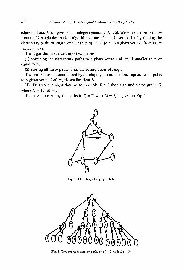
edges in it and L is a given small integer (generally, L < 5). We solve the problem by running N single-destination algorithms, once for each vertex, i.e. by finding the

elementary paths of length smaller than or equal to L to a given vertex i from every

vertex j, j > i. The algorithm is divided into two phases:

(1) searching the elementary paths to a given vertex i of length smaller than or equal to L;

(2) storing all these paths in an increasing order of length.

The first phase is accomplished by developing a tree. This tree represents all paths to a given vertex i of length smaller than L.

We illustrate the algorithm by an example. Fig. 3 shows an undirected graph G,

where N = 10, M = 14. The tree representing the paths to i( = 2) with L( = 3) is given in Fig. 4.

Fig. 3. lo-vertex, 14-edge graph G.

Fig. 4. Tree representing the paths to i ( = 2) with L ( = 3).


The second phase is done by associating with each vertex k in the above tree the sets

of vertices defined by

L:(m) = {successors of k from which i is reachable by a path of length m - l},

where m = 1, 2, , L

Particularly,

L!(l) = {i} if i is a successor of k;

L;(m) = $3.

(3)

Now, we explain how to calculate L:(m). This is accomplished by a breadth-first search on the tree created in the first phase. During it, when vertex ih is met at depth h,

its successor vertex ih_ 1 is put in the set L?(h) and so on. At the end, we obtain L:(m)

for each vertex k (k # i).

Next, we explain how to construct a path, from j to i of length h, denoted by

.i=jO, ji,..., j,_,, j, = i with the sets L:(m).

By the definition of L:(m), the following relation holds:

j,++Li’(h-t), t=O,l,..., h. (4)

This relation allows us to construct a path of length h from j to i. j, = j, then by reading L;(h), we obtain the vertexj,. Similarly, by reading Lj’(h - l), we obtain the

vertex j,, and so on. We give an example clarifying this procedure. In Fig. 4, at depth 3 of the tree, we

associate the following sets with the encountered vertices j ( > 2):

L;(3) = {S}, L:‘(3) = {8, 5}, L;(3) = {lo, 3, l}, L;(3) = {S}, L:(3)

= {10,6), L:(3) = (5).

Similarly, at depth 2, we have

L:‘(2) = {6}, L:(2) = 13, lo>, L;(2) = {3}, L;(2) = {lo}, L;(2)

= (6, lo}, L;(2) = (71, L:(2) = (10).

And at depth 1, we have

LiO(l) = (2}, L;(l) = (2}, L;(l) = {2}, L:(l) = (2).

From the above sets, we can find all the elementary paths from j to 2 (j > 2) of maximal length 3. For example, if we look for the paths from 10 to 2, we begin by constructing the paths from 10 to 2 of length 1. Since L:‘(l) = {2}, there exists a path from 10 to 2.

Similarly, in constructing the paths from 10 to 2 of length 2, L:‘(2) = {6}, L;(l) = {2}, thus we have a path 10 + 6 + 2.

Finally, in constructing the paths from 10 to 2 of length 3, L:‘(3) = {8,5}, L:(2) = (3, lo}, L:(l) = {2}, L:‘(l) = {2}, then we have the first path: 10 + 8 + 3 + 2, the


second path: 10 + 8 + 10 + 2. L;(2) = (6, lo}. L:(l) = {2}, L:‘(l) = {2}, we have the

third path: 10 -+ 5 + 6 + 2 and the fourth path: 10 + 5 + 10 -+ 2. The drawback of this algorithm is the risk of constructing a path having a cycle in

the case of a path j = j,, ji, . . . , jp, . . . , j,, . ,j, = i where jP E L+(h - q). It could happen when L - 2 is greater than the shortest path between j and i. In the above

example, when we search the paths from 10 to 2 of length 3, we obtain two paths

having a cycle: 10 +8--t lo-2 and lo-+5 + 10-2. To avoid this, we test the existence of a cycle during the construction of a path.

We have proposed an optimal data structure to store the sets L:(m) associated with paths. The advantage of this data structure is that it uses little memory

space and allows direct access to a path. In addition, it may be potentially

distributed.

4.2. Data structures

We create a linked data structure to represent L{(m) = {iI, iz, . . . , i,,} as shown in the

Fig. 5. Each element in this representation is an object x called NODE with two data fields:

intl and int2, and two other pointer fields: prev and next. The pointer field next is used

to make up a linked list. In Fig. 5, the NODE x at the first level is called path-node: intl [x] is the vertex j. The

linked list at the second level is called length&t: intl [x] is the length of paths. The

linked list at the third level is called successor-list: intl [x] is a successor it of the vertex j, int2[x] is the edge corresponding to (j, it), and preu[x] points to the length-list of Li’(m - 1).

With this representation, the paths from j to i (i given and j > i) can be constructed

by linking the path-nodes. Fig. 6 represents the structure corresponding to the paths from j to 2 of the graph G.

We have analysed the memory space complexity in the worst-case. In this case, the size of length-list is L(L is the maximal length of paths) and the size of successor-list is

path-node

length-list

Fig. 5. Data structure of L;(m).


Fig. 6. Representation of paths from j to 2.

D (D is the maximal degree of vertices). Number-nodes(i), the number of the NODES used to store the paths from j to i are computed below:

Number-nodes(i) = (1 + L + LD)N. (5)

Doing the same for the vertices i = 1,2, . . , , N - 1, the total number of NODES used

ior G is then (I + f, + LD)N2.

5. Probabilistic calculation: Stratified sampling [lS]

In telecommunication networks, the components are highly reliable, we can thus neglect the states with more thanf failures (j-will be taken equal to 7 or 8 in general).

Let m be the number of components in the network, the network has 2” states.

These states can be divided into m + 1 classes: class Co containing the state without failures where the lost traffic is minimal and equal to zero, class C1 containing states with one failure, . . . , class C, containing states with m failures where the lost traffic is maximal. If we only consider the first f + 1 classes, the upper and lower interval bounds for the calculated measures are

Expected_lost_trafJic,,, = i$l P(Ci)Expected_lost_trafJic(C;),

Expected_lost_trafJic,, = f: P(Ci)Expected_ht_trafJic(Ci) i=l

+ (1 - ii P(C,)) Expected_lost_traJic(C,),

72 J. Carlier ei al. / Discrete Applied Mathematics 76 (1997) 61-80

Availability,,, = i Availability( i=O

Availability,, = 1 - i (P(Ci) - Availability(C i=O

We have used a simulation procedure called stratijied sampling or stratification

[9,6] to calculate the expected lost traffic for classes Ci. The stratified sampling

approach leads to computational savings of several orders of magnitude and is well suited for very large networks which have high component reliability.

5.1. Principle of the stratified sampling

Given a population 52 and a random variable X representing a characteristic of the

population, we want to estimate the mean m of X. The stratified sampling consists in dividing the population Sz into k subpopulations

as homogeneous as possible: Q1, &, . . . , !Sk. These subpopulations are called strata.

They are not overlapping, and their union is equal to the population, i.e., &+s22+ ..’ +52,=52.

Each unit hi in the stratum Oh has a probability phi, and the probability Ph of sZh is the sum of ph,, we have xi=, P,, = 1.

We distinguish equiprobable and non-equiprobable strata. If phi in the Q, are different, this stratum is called non-equiprobable, otherwise, equiprobable. The main difficulties arise for the case of strata non-equiprobable.

When the strata have been determined, a sample nh is independently drawn from each of them. The sample sizes within the strata are denoted by nr, n2, . . . , nk,

respectively. n is the total size of the stratified sample n = nl + n2 + ... + nk. (1) Stratljied estimate zStr. The estimate for m in stratified sample is

&,, = ; PhXh, h=l

where

The main properties of the estimate s,,, are outlined in [6]. (2) Conjidence intervals. The confidence intervals are as follows:

IL - 5S(XSA L + LNL)I

where

(7)

(8)

P(R,,,) = 5 Pi5 2, s; = h=l

--& ,i (xhi - xh)'. r-l

J. earlier et al. / Discrete Applied Mathematics 76 (1997) 61-80 13

These formulae assume that X,,, is normally distributed so that the multiplier 5 can be read from tables of normal distribution, but they can also be applied in the general

case when nh 2 25, for every h.

5.2. Estimation of the availability and the lost trafJic

We return to the model presented in Section 3, the states of a component i can be represented by a Bernoulli distributed random variable Xi with parameter

Pi = Pi/(4 + Pi),

Xi= 1, ,component i is in operating statej .

A network state is represented by a random variable vector X = (XI, X2, . . ,X,), and its values x = (x1, x 2, . . . ,x,) has a probability

P(X = X) = n pi n (1 - pi). i/x, = 1 i/xi = 0

We use two other random variables to represent, respectively, the two network

characteristics: Y(x) the lost traffic in state x, and Q(x) the structure function of system defined by

Q(x) = i

1 if a(x) > z,

0 otherwise.

Hence, the expected lost traffic and the availability are the means of the random variables Ii/(x) and Q(x):

Expected_lost-trafic = E(Y(X)) = 1 Y(x)P(X = x), xeR

Availability = E(@(X)) = 1 @(x)P(X = x). XCQ

(9)

Our problem is thus to estimate E(@(X)) and E(Y(X)). Our method consists in first dividing the network state into strata. For a small

stratum, that is, containing a few of states, we exactly calculate it by complete

enumeration; otherwise, we estimate it by drawing a sample. By the result presented in Section 5.1, the estimates for the expected lost traffic and the availability can be rewritten as

- Expected_lost_trafJic, = i P,, Y(X),,

h=l

where

(10)

Availability, = i P,, Q(X),, ,

h=l

14 J. Carlier et al. J Discrete Applied Mathematics 76 (1997) 61-80

where

Q(x), = Lh @(x) nh

5.3. Problems to dove

The following five problems have to be solved in order to estimate the expected lost

traffic and the availability: (1) define the strata Qh, (2) determine the sizes nh of samples corresponding to the total size it of the

stratified sample, (3) estimate the total sample size n corresponding to the calculation accuracy y, (4) draw a random sample q# in a stratum fib,

(5) calculate the probability Ph of a stratum &. The second and the third problems have been solved by Cochran [6]. We report

here their solutions. In the stratified sampling to minimize the variance, the values of the sample sizes nh in the respective strata for a specified size n of the sample are given

by

(11)

In order to obtain the calculation accuracy y, n has to be chosen by the formula

n = (CPhah)2 t2

(v4’

where m is the mean of X. (12)

In the following paragraphs, we treat the remaining problems.

5.3.1. Dejinition of strata We have to define the strata so that they are as homogeneous as possible. The

variance of estimates of each stratum must be small in order to minimize the variance of the stratified sample.

A simple definition of a stratum is given by a triple (u, v, w). The stratum (u, v, w) regroups all network states with u failed system arcs, v failed cables and w failed nodes. For example, for a class with 3 failures, we have the first stratum containing the states with 3 link failures, the second stratum containing the states with 2 link failures and 1 cable failure, . . .

Other definitions are possible, which is a perspective of our work.

5.3.2. Drawing of a sample q, in the stratum 52, The elementary way of drawing in statistics is the random sampling. In any draw,

the drawing must fulfill the unit probability in a population. This probability is the

J. earlier et al. 1 Discrete Applied Mathematics 76 (1997) 61-80 75

same for all units when strata are equiprobable. In this case, the sample obtained is called simple random sample. When strata are not equiprobable, it is necessary to apply other methods for drawing a sample. We use a simple and efficient method called the method ofreject [ 161 whose essential idea is to use a second drawing so that

a unit having a greater probability has a greater chance of being drawn. Concretely, by the method of reject, we first draw randomly a unit e from a non-

equiprobable stratum L$, and we calculate its probability p(e). Then, we draw randomly a number a in the interval [0, maxxprob], max-prob being the maximum of

probabilities of states in Q,,. If a 6 p(e), e is kept in the sample to constitute; otherwise, e is rejected. This process is repeated until a random sample rc,, is constituted.

5.3.3. Calculation of the probability Ph of the stratum Q,, In the case of an equiprobable stratum, Ph is equal to the probability of a network

state in stratum Q,, multiplied by the number of states of Q,,. In the case of a non- equiprobable stratum, a classic method is to compute Ph by enumerating all combinations of arcs, cables and nodes. However, this enumeration demands an exponential time. This is inapplicable for a large network. We propose instead a quadratic

algorithm for computing P,,.

The principle of this algorithm is to decompose Ph into a product of several terms corresponding to subtrees, and to calculate the probability of each subtree in a quad-

ratic time. Note that the causes of failures are supposed to be independent. This algorithm consists of two steps.

(1) Decomposition of Ph. It can be easily verified that

P,, = probw * sum_noe*sum_cab*sum_sys (13)

with

probw = n py fl pyb i=l i=l i=l

where nnoe, ncab and nsys note, respectively, the numbers of nodes, cables and system arcs, and pnoe, pcab and psys, respectively, the number of node failures, cable failures and system arc failures. sum-cab and sum_noe are given by formulae similar to sum_sys (13).

This step is illustrated by combination of subtrees that corresponds to the terms. We give an example: with nsys, ncab and nnoe, respectively, equal to 6,4,4, we consider a stratum (2,2, 1) with 2 link failures, 2 cable failures and 1 node failure. We enumerate all combinations of these 5 failures using the tree of Fig. 7.

(2) Calculation of the probability of a subtree: We state now a recursive formula which allows to calculate sum-noe, sum-cub and sum-sys in a quadratic time.


node failure enumeration

arc failure enumeration

Fig. 7. Tree corresponding to the enumeration of failures.

Let us define

then

n-j+1

(14)

where n is the number of a given type components, p is the number of a given type component failures, and j = 0, 1, . . . ,p -

For example,

1, p. Particularly, II”, = 1.

n = nsys, p = psys,

Hence, sum__sys can be rewritten by -

With I7”, = 1, we calculate II”, = Ci=, ah at the beginning, and we obtain II: at the end, that is, we calculate sum-sys, sum-cub and sum-we.

This calculation procedure may be schematized by Fig. 8.

J. Carlier et al. / Discrete Applied Mathematics 76 (1997) 61-80 II

n- +2 P- P

n1 A . . . . . .

a an

1 n+l . . . . . . 0 . . . . . .

Fig. 8. A subtree corresponding to the calculation of II!.

By developing formula (14), we have the following results for the example in Fig. 7:

(16)

By taking into account the two steps, it is clear that the computing time is proportional to

O(max(pnoes,pcab,psys)Xmax(nnoe,ncab,nsys)) (17)

It is substantially reduced in comparison with the exponential time of the complete enumeration. Now, the strata probability P,, can be calculated in quadratic time.


6. Computational results

We have implemented a prototype program which allows to calculate confidence

intervals of the expected lost traffic and the availability by using the stratified sampling method. We present below two groups of experiments realized on SUN Station Spare 2.

(1) Validity ofthe method: in order to compare the results obtained by the stratified

sampling and the exact results, we have tested our program on a network of 26 nodes [12] by limiting the number of failures to 2. We present some results in Table 2.

(2) Applying the method to a large network: Table 3 gives the result of one proced-

ure on a network of 114 nodes [12].

Table 2

Exact results Estimated results

Max path Lost-traffic Availability Time Lost-traffic Availability Time Length (L) (s) (s)

5 69.801632 0.669807 24.8 [67.604659,71.573623] [0.665825,0.676690] 1 6 55.299030 0.708848 39.2 [53.293667,57.101423] [0.705753,0.717841] 14.8 7 47.323774 0.748539 59.6 [45.312288,49.041037] [0.745647,0.756886] 22.0 8 42.798904 0.773666 92.2 [40.803806,44.522097] [0.770184,0.780955] 32.3 9 39.447225 0.791327 144.0 [37.470540,41.174457] [0.787292,0.798033] 47.1

10 34.205541 0.827880 212.6 [32.248436,35.961330] [0.824734,0.835207] 69.4

Table 3

Number of nodes = 114 Number of cables = 179 Number of systems = 183

Sum of spare capacity = 132713 Sum of working capacity = 144 187

Probability of node from 0.98039 to 0.98901 Probability of cable from 0.99800 to 0.99889 Probability of system from 0.99980 to 0.99987

Maximum length of paths for rerouting (L) = 5 Number of failures considered (f) = 8

Availability coefficient (z) = 0.98 Probability of confidence for intervals = 0.99

Results

Cumul probability = 0.994371 Probability without failure = 0.048330 Total availability = 0.854072 Total traffic demands = 69563.000000 Total lost traffic = 645.754303 Confidence intervals over states with at most 8 failures Expected-lost-traffic = [619.0136,672.4949] Availability = [0.844873,0.863270]

Intervals over all states Expected-lost-traffic = [619.01,1064.05] Availability = [0.844873,0.868899] Computing time 674.4 s


7. Conclusion

We have presented a method based on K-shortest path rerouting and stratified sampling technique to calculate the reliability of telecommunication networks. The

rerouting is made very rapidly, thanks to a sophisticated data structure. The stratified

sampling method especially takes into account the case of non-equiprobable strata. The main interest of our method is that it is effective in practice for very large networks (e.g. a network of 100 nodes). Up to now, we have not seen any work done

with such a result. Moreover, this method is very general: it can be used to calculate

other characteristics of network reliability.

Acknowledgements

This work was supported by the Centre National d’Etudes des Telecommunica- tions (grant N”7758c).

References

[l] A. Aggarwal and R.E. Barlow, A survey of network reliability and domination theory, Oper. Res. 32 (1984) 478-479.

[2] R.J. Boehm, Y.C. Ching, C.G. Griffith and F.A. Saal, Standardized fiber optic transmission systems ~ a synchronous optical network view, IEEE J. Select. Areas Comm. SAC-4 (1986) 142441431.

[3] J. Carlier, Y. Li and J.-L. Lutton, Evaluation of telecommunication network performances, in: J. Henry and J.-P. Yvon, eds. Proceedings of the 16th IFIP-TC7 Conference on System Modelling and Optimisation, France, 5-9 July 1993, Lecture Notes in Control and Information Sciences, vol. 197 (Springer, Berlin 1994) 865-874.

[4] J. Carlier, Y. Li and J.-L. Lutton, Reliability evaluation of large telecommunication networks by using stratification method, Proceedings of the 6th International Network Planning Symposium NETWORKS’94, Hungary, 5-9 September (Scientific Society for Telecommunications, 1994) 113-118.

[S] J. Carlier and C. Lucet, A decomposition method for network reliability evaluation, Discrete Appl. Math. (1995) 1768.

[6] W.G. Cochran, Sampling Techniques (Wiley, New York, 1977). [7] D.A. Dunn and W.D. Grover, Comparison of k-shortest paths and maximum flow routing for

network facility restoration, IEEE J. Selected Areas Commun. 12 (1994) 88-99. [S] S. Even, Graph Algorithms. (Computer Science Press, Rockville, MD, 1979). [9] H. Frank, Survivability analysis of command and control communications networks - Part II, IEEE

Trans. Commun. 22 (1974) 596-605. [lo] W.D. Grover, The selfhealing network: a fast distributed restoration technique for networks using

digital cross-connect machines, IEEE Global Telecommunication Conf. (1987) 28.2.1-28.2.6. [l l] W.D. Grover, T.D. Bilodeau and B.D. Venables, Near optimal spare capacity planning in a mesh

restoration network, IEEE Global Telecommunication Conf. (1991) 57.1.1-57.1.6. [12] Y. Li, Etude et calcul de la fiabilitt des reseaux de telecommunication, PhD Dissertation, Universitb

de Technologie de Compiegne, France, 1993. [ 133 M.O. Locks, Recent development in computing of system reliability, IEEE Trans. Reliab. 34 (1985)

4255436. [14] C. Palmer and F. Hummel, Restoration in a partitioned multi-bandwidth cross-connect network,

1EEE Global Telecommunication Conf. (GLOBECOM) (1990) 301.7.1-301.7.5.

80 J. Carlier et al. 1 Discrete Applied Mathematics 76 (1997) 61-80

[15] B. Sanso, F. Soumis and M. Gendreau, On the evaluation of telecommunication networks reliability using routing models, IEEE Trans. Commun. 39 (1991) 1494-1501.

[16] G. Saporta, Probabilites, analyse des don&s, et statistique (Editions Technip, Paris, 1990). [17] F. Soumis and B. Sanso, Communication and transportation network reliability using routing

models, IEEE Trans. Reliab. 40 (1991) 29-38. [18] 0. Theologou and J. Carlier, Factoring and reductions for networks with imperfect vertices, IEEE

Trans. Reliab. 40 (1991) 210-217.

reliability evaluation of large telecommunication networks · makes possible a rapid restoration...

Documents