Reliability based design of flood defenses and river dikes P.H.A.J.M. van Geldera, and J.K. Vrijlinga

aFaculty of Civil Engineering and Geosciences, University of Technology Delft, The Netherlands, email: p.vangelder@ct.tudelft.nl, and j.k.vrijling@ct.tudelft.nl

Abstract In this paper an example is elaborated of the design of a river dike, incorporating reliability-based models. The design is demonstrated with the help of this example, which is based on [1].

1. PROBLEM DESCRIPTION

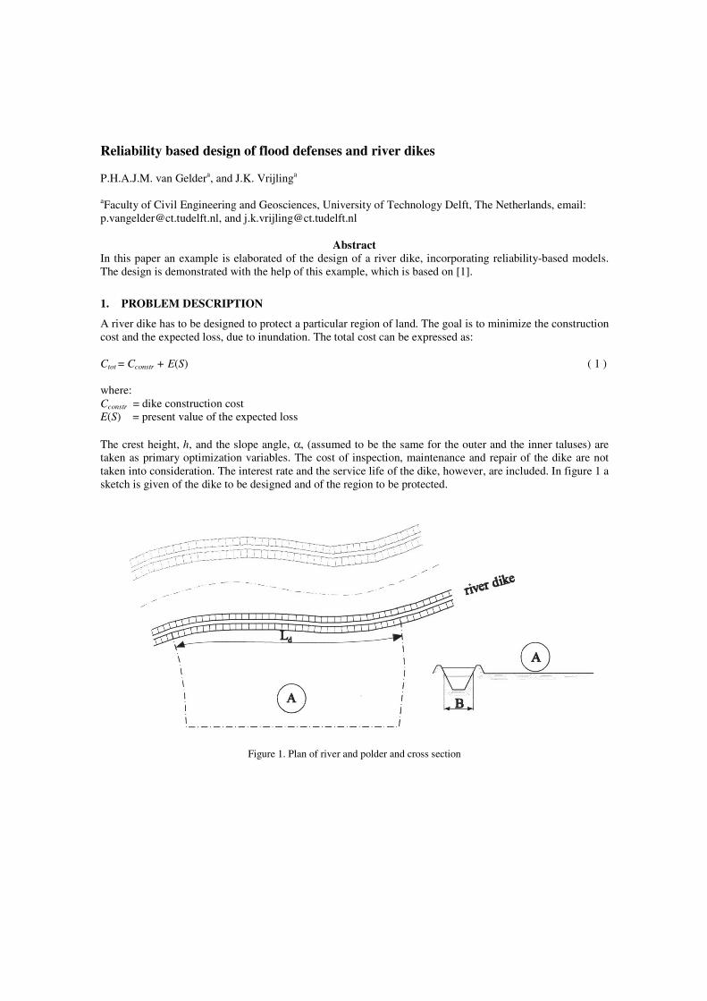
A river dike has to be designed to protect a particular region of land. The goal is to minimize the construction cost and the expected loss, due to inundation. The total cost can be expressed as: Ctot = Cconstr + E(S) ( 1 ) where: Cconstr = dike construction cost E(S) = present value of the expected loss The crest height, h, and the slope angle, α, (assumed to be the same for the outer and the inner taluses) are taken as primary optimization variables. The cost of inspection, maintenance and repair of the dike are not taken into consideration. The interest rate and the service life of the dike, however, are included. In figure 1 a sketch is given of the dike to be designed and of the region to be protected.

Figure 1. Plan of river and polder and cross section

River It is assumed that one single flood wave raising the water level in the river once throughout a year poses the only hazard to the dike. The shape of this flood wave in time, presented in figure 2, is parabolic. The river width, B, is assumed to be constant, being 400 m. The bottom level of the river, hh , is 3.5 m below datum level. The gradient of the river bed, I, is 10-4, whereas De Chezy’s constant is taken as C = 40 m1/2 s-1.

Figure 2. Shape of the flood wave and indication of the water level

River dike The length of the river dike, Ld , is 20 km. Its schematized cross section (not to scale) is shown in figure 3. The cross section is symmetrical in shape. The dike consists of a sand core, the outer talus of which is covered with clay. The crest is at a level h0 above datum level, the crest width is bk and the base width is L2. The subsoil consists of sand, covered with a clay layer thick dk = 3.5 m. The taluses slope with angles α with the horizontal. If necessary a foreland can be created on the outer side of the dike (i.e. river ward) by building the dike further inland. The width of the foreland then is L1.

Figure 3. Cross section of the river dike

Protected region The protected area, A, covers 200 km2. Its level, hm , is supposed to be entirely at 0.5 m above level datum. Part α1 of the region is urban area (α1

.A km2), α2.A km2 is used for agriculture and the α3

.A km2

remainder, is industrial area. The coefficients, α1 , α2 and α3 are taken as 0.06, 0.93 and 0.01 respectively. The region is assumed to contain no flood water retaining provisions, neither intended nor accidentally present. Considered failure mechanisms Failure of flood defences can be adequately modelled with help of fault trees (Vrijling, 2001). In this paper, it is assumed that inundation of the protected area can be caused in two ways:

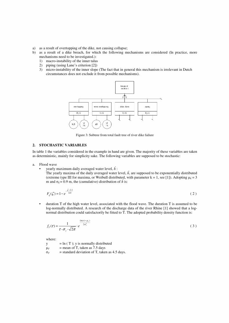
a) as a result of overtopping of the dike, not causing collapse; b) as a result of a dike breach, for which the following mechanisms are considered (In practice, more

mechanisms need to be investigated.): 1) macro-instability of the inner talus 2) piping (using Lane’s criterion [2]) 3) micro-instability of the inner slope (The fact that in general this mechanism is irrelevant in Dutch circumstances does not exclude it from possible mechanisms).

Figure 3: Subtree from total fault tree of river dike failure

2. STOCHASTIC VARIABLES

In table 1 the variables considered in the example in hand are given. The majority of these variables are taken as deterministic, mainly for simplicity sake. The following variables are supposed to be stochastic: a. Flood wave • yearly maximum daily averaged water level, ĥ :

The yearly maxima of the daily averaged water level, ĥ, are supposed to be exponentially distributed (extreme type III for maxima, or Weibull distributed, with parameter k = 1, see [1]). Adopting µĥ = 3 m and σĥ = 0.9 m, the (cumulative) distribution of ĥ is:

2.1

0.9ˆ ( ) 1h

F eζ

ζ−−

= − ( 2 )

• duration T of the high water level, associated with the flood wave. The duration T is assumed to be

log-normally distributed. A research of the discharge data of the river Rhine [1] showed that a log-normal distribution could satisfactorily be fitted to T. The adopted probability density function is:

2

(ln( ) )

21( )

2

y

y

T

y

f e

τ µ

σττ σ π

−

= ⋅⋅ ⋅

( 3 )

where:

y = ln ( T ); y is normally distributed µT = mean of T, taken as 7.5 days σT = standard deviation of T, taken as 4.5 days.

b. Soil The following parameters of clay and sand are assumed to be stochastic:

k = permeability [m/s] φ = angle of natural slope [O]; c’ = cohesion [kN/m] λeq = kk,eq / dk,eq = equivalent leakage factor of the clay layer on the outer talus, including the

perforations in this layer kk,eq = equivalent permeability of clay dk,eq = equivalent thickness of the clay layer (see below)

In an actual case it is sometimes possible to provide a statistical basis for some variables, but for other variables it will be necessary to rely on estimates.

c. Geometry • Thickness of clay layer on outer talus.

The permeability of the clay layer on the outer talus is important as it is a determining factor in the position of the phreatic surface. The effect of a variation in thickness is combined with the permeability of the clay to the equivalent leakage factor: λeq= kk,eq / dk,eq ( 4 )

• Thickness of clay layer under the dike. The clay layer on which the dike is situated, varies in thickness. It is modelled by a layer of constant but unknown thickness, which is normally distributed with mean 3.5 m and coefficient of variation of 0.2.

d. Model factor for piping

In the piping mechanism a model factor is introduced as (among other things) to represent the variation in the results. Lane’s formula [2] is chosen to model piping (being a “conservative” assumption compared with Sellmeijer’s [3] formulation). The model factor is supposed to be a normally distributed variable with mean 1.67 and coefficient of variation 0.2.

e. Width of the breach

The width of the breach in a dike, b , may vary greatly [4]. The distribution is assumed to be of log-normal type. The mean width is taken as 100 m and the coefficient of variation as 1.0.

Table 1 Overview of the problem variables

variable description type µ unit σ / µ ĥ highest water level (upstream) E 3 m 0.30 T duration of high water level LN 7.5 days 0.60 ck cohesion (clay) N 10 kN/m2 0.20 φk angle of repose (clay) N 20 degrees 0.20 kk permeability (clay) LN 10 -8 m/s 1.60 cz cohesion (sand) D 0 kN/m2 - φz angle of respose (sand) N 35 degrees 0.10

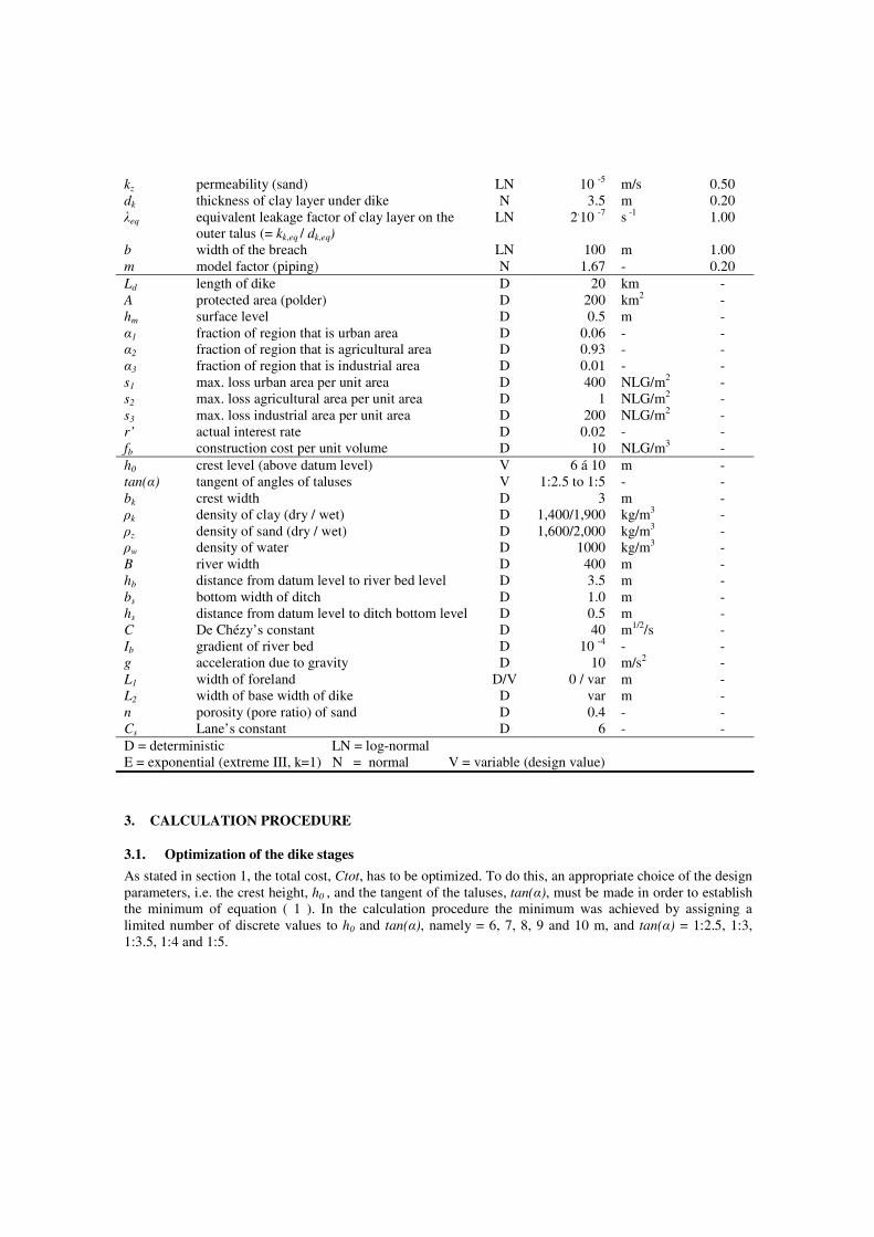
kz permeability (sand) LN 10 -5 m/s 0.50 dk thickness of clay layer under dike N 3.5 m 0.20 λeq equivalent leakage factor of clay layer on the

outer talus (= kk,eq / dk,eq) LN

2.10 -7 s -1 1.00

b width of the breach LN 100 m 1.00 m model factor (piping) N 1.67 - 0.20 Ld length of dike D 20 km - A protected area (polder) D 200 km2 - hm surface level D 0.5 m - α1 fraction of region that is urban area D 0.06 - - α2 fraction of region that is agricultural area D 0.93 - - α3 fraction of region that is industrial area D 0.01 - - s1 max. loss urban area per unit area D 400 NLG/m2 - s2 max. loss agricultural area per unit area D 1 NLG/m2 - s3 max. loss industrial area per unit area D 200 NLG/m2 - r’ actual interest rate D 0.02 - - fb construction cost per unit volume D 10 NLG/m3 - h0 crest level (above datum level) V 6 á 10 m - tan(α) tangent of angles of taluses V 1:2.5 to 1:5 - - bk crest width D 3 m - ρk density of clay (dry / wet) D 1,400/1,900 kg/m3 - ρz density of sand (dry / wet) D 1,600/2,000 kg/m3 - ρw density of water D 1000 kg/m3 - B river width D 400 m - hb distance from datum level to river bed level D 3.5 m - bs bottom width of ditch D 1.0 m - hs distance from datum level to ditch bottom level D 0.5 m - C De Chézy’s constant D 40 m1/2/s - Ib gradient of river bed D 10 -4 - - g acceleration due to gravity D 10 m/s2 - L1 width of foreland D/V 0 / var m - L2 width of base width of dike D var m - n porosity (pore ratio) of sand D 0.4 - - Cs Lane’s constant D 6 - - D = deterministic LN = log-normal E = exponential (extreme III, k=1) N = normal V = variable (design value)

3. CALCULATION PROCEDURE

3.1. Optimization of the dike stages

As stated in section 1, the total cost, Ctot, has to be optimized. To do this, an appropriate choice of the design parameters, i.e. the crest height, h0 , and the tangent of the taluses, tan(α), must be made in order to establish the minimum of equation ( 1 ). In the calculation procedure the minimum was achieved by assigning a limited number of discrete values to h0 and tan(α), namely = 6, 7, 8, 9 and 10 m, and tan(α) = 1:2.5, 1:3, 1:3.5, 1:4 and 1:5.

3.2. Construction cost

The cost of the dike is assumed to depend on the volume of the dike body only. The equation expressing the construction cost is: Cconstr = Ld

. h0 . (h0

. cotan(α) + bk ) . fb ( 5 )

in which: Ld = length of dike h0 = crest height (above datum level), design parameter cotan(α) = cotangent of the slope of the inner and outer talus, design parameter bk = crest width fb = construction cost per unit volume.

3.3. Present value of the risk

Inundation will occur upon failure of the dike. The result will be a particular amount of damage or loss, S, which is assumed to depend only on the inundation depth, d. The risk in year i, or the expectation of the loss in year i is: E(S)i = P(Fi)

. S ( 6 ) where: P(Fi ) = probability of failure in year i S = amount of damage or loss. Considering the actual interest rate and the intended service life of the dike, the capitalized loss expectation, or the present value of the risk, can be written as:

,1

( )( )

(1 )

Ni

ii

P F SE S

r=

⋅=

+∑ ( 7 )

in which: N = intended service life r’ = actual interest rate. If N is large and P(Fi ) is constant in time, E( S) can be written as:

,

( )( ) iP F S

E Sr

⋅= ( 8 )

or:

,0

1( ) ( ) ( )dE S S d f d

rδ δ δ

∞

= ⋅ = ⋅ ⋅∫ ( 9 )

where: fd(δ) = probability density function of the inundation depth, d (figure 5).

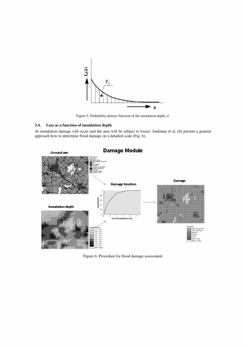
Figure 5. Probability density function of the inundation depth, d.

3.4. Loss as a function of inundation depth

At inundation damage will occur and the area will be subject to losses. Jonkman et al. [6] present a general approach how to determine flood damage on a detailed scale (Fig. 6).

Figure 6. Procedure for flood damage assessment

δ

f d(δ

)

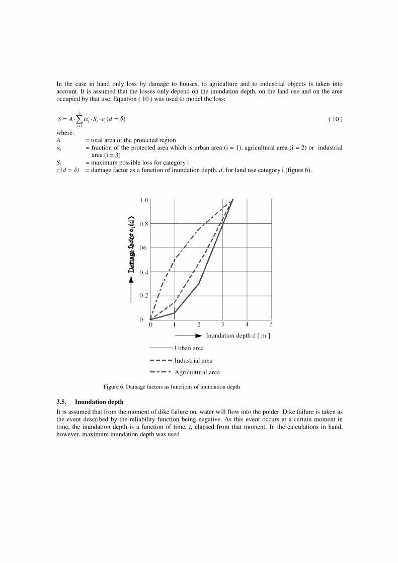
In the case in hand only loss by damage to houses, to agriculture and to industrial objects is taken into account. It is assumed that the losses only depend on the inundation depth, on the land use and on the area occupied by that use. Equation ( 10 ) was used to model the loss:

3

1

( )i i ii

S A S c dα δ=

= ⋅ ⋅ ⋅ =∑ ( 10 )

where: A = total area of the protected region αi = fraction of the protected area which is urban area (i = 1), agricultural area (i = 2) or industrial

area (i = 3) Si = maximum possible loss for category i ci(d = δ) = damage factor as a function of inundation depth, d, for land use category i (figure 6).

Figure 6. Damage factors as functions of inundation depth

3.5. Inundation depth

It is assumed that from the moment of dike failure on, water will flow into the polder. Dike failure is taken as the event described by the reliability function being negative. As this event occurs at a certain moment in time, the inundation depth is a function of time, t, elapsed from that moment. In the calculations in hand, however, maximum inundation depth was used.

Given the equations for ci(d=δ), the area of the polder, A, the fractions of land use, αi, and the maximum possible loss for land use category i, s , the loss, S, can be calculated as a function of the inundation depth. To calculate E(S) from equation ( 9 ), the probability density function, fd(δ), has to be established. This can be done by determining the probability P{d>δ AND failure} for a number of values of δ. In principle the probability density function, fd(δ) , can then be calculated:

( ) { } { }( ) d

d

dF P d P df

d

δ δ δ δδδ δ

> − > + ∆= =∆

( 11 )

The probability P{d > δ} was calculated according to level II analyses a by FORM approach (it can be refined by SORM- calculations which were not performed in the example in hand.) In calculating P{d > δ} it is implicitly assumed that the dike fails. The results of FORM-calculations therefore result in: P { d > δ AND failure } ( 12 )

3.6. Computational scheme

The calculation procedure of a mechanism basically consists of the successive determination of each design combination (h0 , tan(α)): • the probability of failure P{Zi < 0} • P{Z0 < 0} = P{d > δ} for the various values of δ (0.25 - 3.5 m) • the correlation coefficient ρ(Z0Zi) for the various values of δ • the probability P { d > δ AND Zi < 0 } ~=~ Fd(δ) • the probability density function fd(δ) • the present value of the risk, E(S) according to equation ( 9 ) • the construction cost, Cconstr , according to equation ( 5 ) • the total cost Ctot = Cconstr+ E(S), according to equation ( 1 ). The actual optimum can only be determined if the mechanisms are combined. Primarily, the mechanisms are dealt with separately.

4. RESULTS PER MECHANISM

4.1. Overtopping

In figure 7 the mechanism of overflowing is schematically illustrated. The following steps in the calculation are considered:

Figure 7. Mechanism of overtopping

a. Failure probability

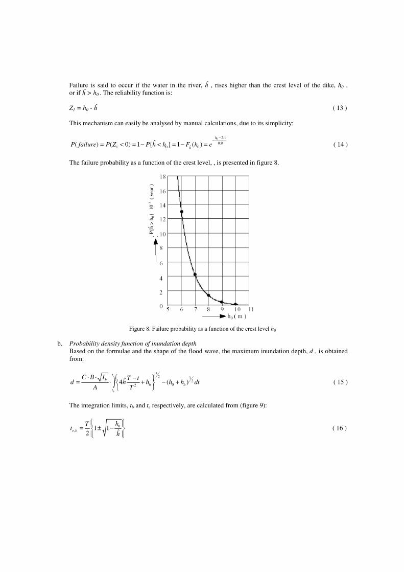
Failure is said to occur if the water in the river, ĥ , rises higher than the crest level of the dike, h0 , or if ĥ > h0 . The reliability function is: Z1 = h0 - ĥ ( 13 ) This mechanism can easily be analysed by manual calculations, due to its simplicity:

0 2.1

0.9ˆ1 0 0

ˆ( ) ( 0) 1 { } 1 ( )h

hP failure P Z P h h F h e

−−

= < = − < = − = ( 14 )

The failure probability as a function of the crest level, , is presented in figure 8.

Figure 8. Failure probability as a function of the crest level h0

b. Probability density function of inundation depth

Based on the formulae and the shape of the flood wave, the maximum inundation depth, d , is obtained from:

32 3

202

ˆ4 ( )e

b

tb

h h

t

C B I T td h h h h dt

A T

⋅ ⋅ − = ⋅ + − + ∫ ( 15 )

The integration limits, tb and te respectively, are calculated from (figure 9):

0, 1 1

ˆ2e b

hTt

h

= ± −

( 16 )

P{ĥ

> h

0} . 1

0-3 (

yea

r )

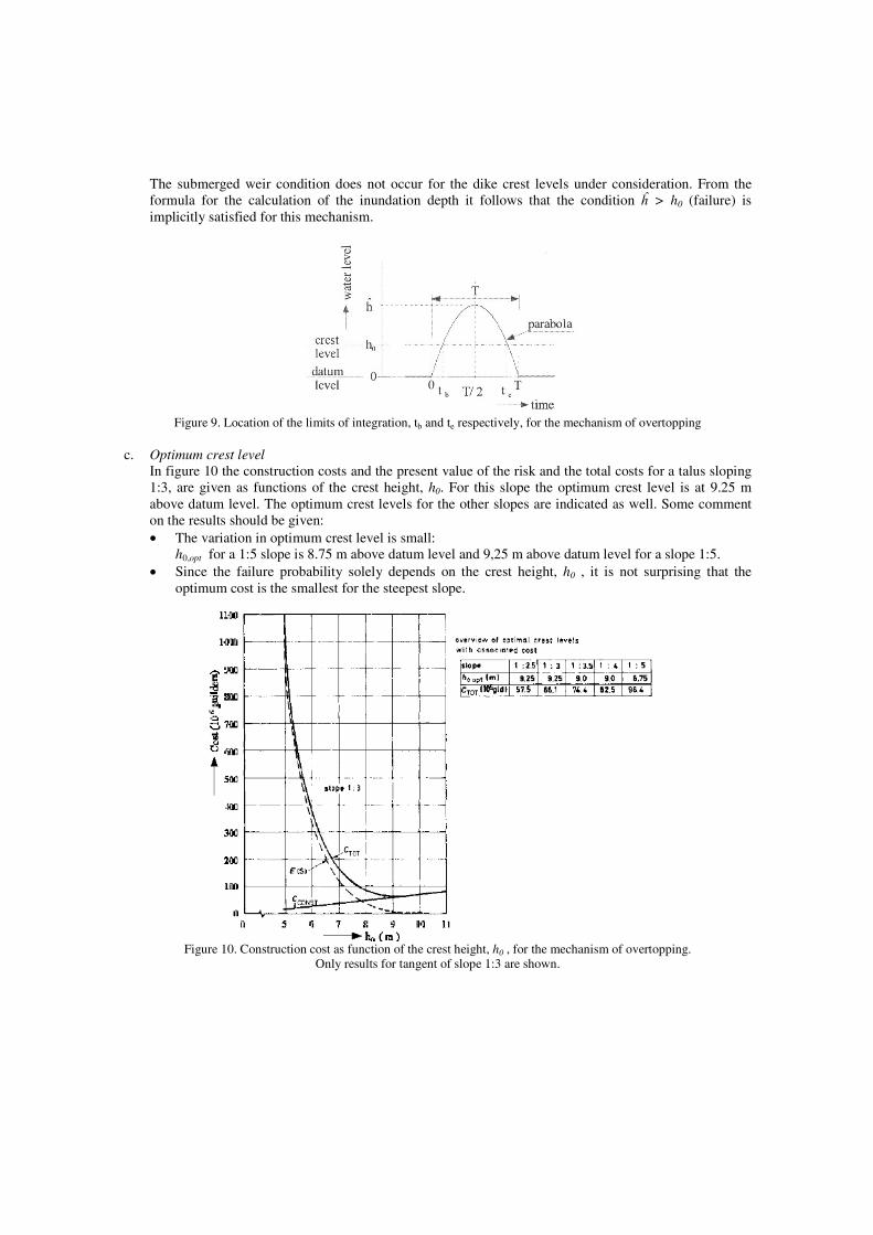
The submerged weir condition does not occur for the dike crest levels under consideration. From the formula for the calculation of the inundation depth it follows that the condition ĥ > h0 (failure) is implicitly satisfied for this mechanism.

Figure 9. Location of the limits of integration, tb and te respectively, for the mechanism of overtopping

c. Optimum crest level

In figure 10 the construction costs and the present value of the risk and the total costs for a talus sloping 1:3, are given as functions of the crest height, h0. For this slope the optimum crest level is at 9.25 m above datum level. The optimum crest levels for the other slopes are indicated as well. Some comment on the results should be given: • The variation in optimum crest level is small: h0,opt for a 1:5 slope is 8.75 m above datum level and 9,25 m above datum level for a slope 1:5. • Since the failure probability solely depends on the crest height, h0 , it is not surprising that the

optimum cost is the smallest for the steepest slope.

Figure 10. Construction cost as function of the crest height, h0 , for the mechanism of overtopping.

Only results for tangent of slope 1:3 are shown.

4.2. Macro-instability of the inner talus

The phreatic surface in the dike is schematized to a straight line. a. Failure probability

The stability factor, Γ , is calculated by some slip surface model. Several methods are known from literature. A well known method is the so called simplified Bishop method.

The critical slip circle is the slip circle for which the stability factor is smallest. The critical slip circle has to be found in an iteration process, changing both the centre and the radius of the slip circle. The “deterministic” stability factor, Γ , for a slip circle follows from equilibrium:

{ }, ,

1

( ) tan( )n

i i ii

R A

R c u bM M

σ ϕ=

+ − ⋅ ∆= =

Γ

∑ , where R

A

M

MΓ = ( 17 )

from which Γ has to be solved in an iterative process. The reliability function can be written as: Z2 = Γ - q ( 18 )

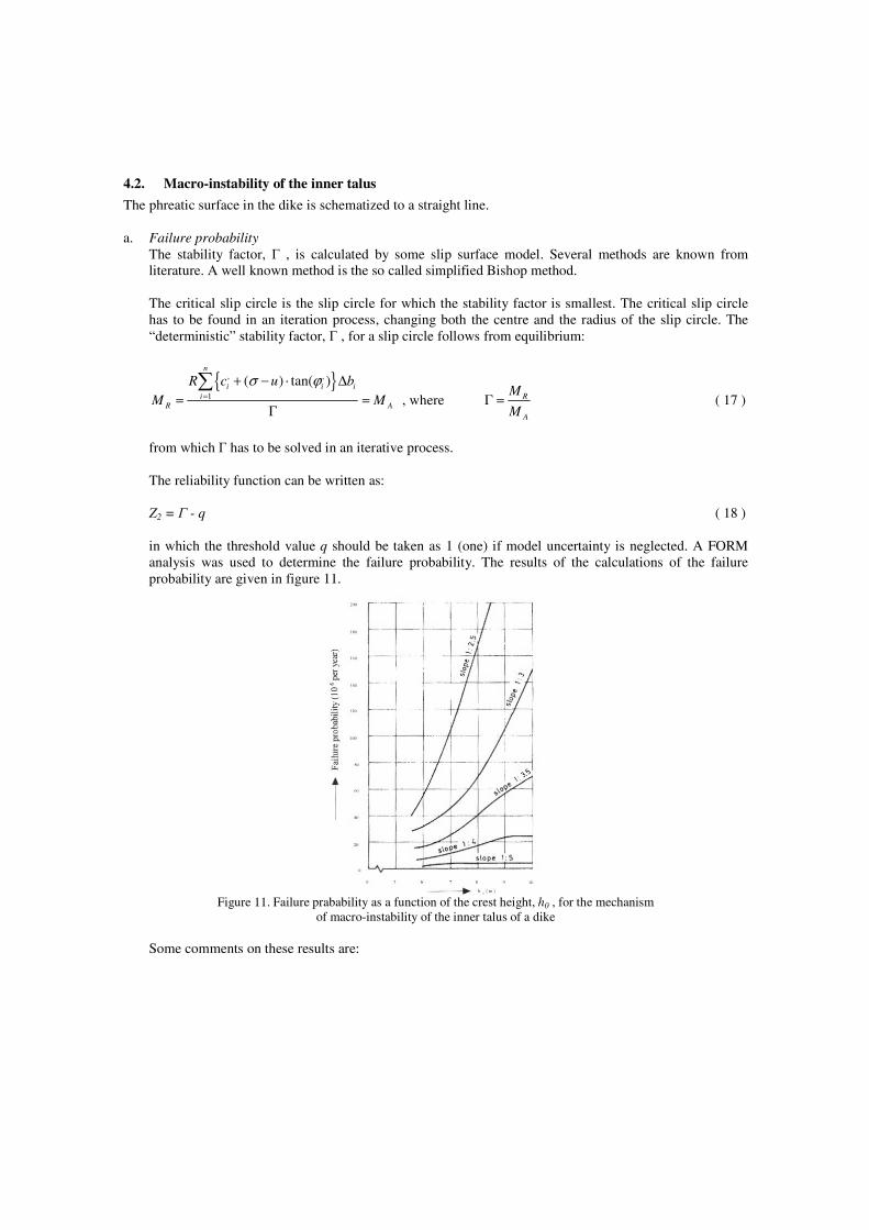
in which the threshold value q should be taken as 1 (one) if model uncertainty is neglected. A FORM analysis was used to determine the failure probability. The results of the calculations of the failure probability are given in figure 11.

Figure 11. Failure prabability as a function of the crest height, h0 , for the mechanism

of macro-instability of the inner talus of a dike Some comments on these results are:

• the calculated failure probabilities are rather low (smaller than 8.10 - 4 per year, except for slope 1:2.5)

• the failure probability increases with increasing cfrest level. Reasons for this are: o the phreatic surface does not effect the governing slip circle for the crest heights and

slopes considered. o the overturning moment increases relatively faster than the resisting moment if the crest

height is increased • if the crest level is increased above a particular level, the failure probability is not influenced

by this increase as no part of the (horizontal) crest is contained in the slip circle. b. Probability density function of inundation depth

For the free-napped weir (no deduction is given here) the maximum inundation depth, d, can be calculated from :

3

22

2 23 3 ( )

e

b

t

m

t

gd b h h dt

A= − ⋅∫ ( 19 )

Water depth h2 can be found from the equation of continuity:

3 1 1

2 2 21 2 2

3 22 3( ) ( ) ( )b m b

b

gh h b h h h h

CB I+ = − + + ( 20 )

The integration limits, and respectively, were taken as: tb = moment at which the river attains its highest water level

te = moment at which overtopping changes from free-nappe to submerged weir. This situation occurs

if 2

2( )

3 md h h= − .

For submerged weir conditions, d can be calculated from:

2

2( ) ( )m

gd d b d h h d dt

A= ⋅ ⋅ − − ⋅ ( 21 )

In this equation ( 21 ), has h2 to be solved from the continuity equation as well:

3 3

2 21 2 2

2( ) ( ) ( )b m b

b

gh h b d h h d h h

C B I+ = ⋅ − − + +

⋅ ⋅ ( 22 )

Solving is done by iteration. The calculation is stopped as soon as d + hm = h2 . c. Optimum crest level

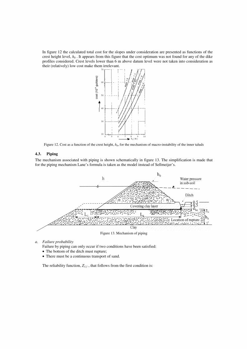
In figure 12 the calculated total cost for the slopes under consideration are presented as functions of the crest height level, h0 . It appears from this figure that the cost optimum was not found for any of the dike profiles considered. Crest levels lower than 6 m above datum level were not taken into consideration as their (relatively) low cost make them irrelevant.

Figure 12. Cost as a function of the crest height, h0, for the mechanism of macro-instability of the inner taluds

4.3. Piping

The mechanism associated with piping is shown schematically in figure 13. The simplification is made that for the piping mechanism Lane’s formula is taken as the model instead of Sellmeijer’s.

Figure 13. Mechanism of piping

a. Failure probability Failure by piping can only occur if two conditions have been satisfied:

• The bottom of the ditch must rupture; • There must be a continuous transport of sand.

The reliability function, Z3,1 , that follows from the first condition is:

cost

(10

-6 g

uild

ers)

3,1 ,ˆ( )nk kd eff w bZ g d g h hρ ρ= ⋅ ⋅ − ⋅ ⋅ + ( 23 )

where: ρnk = density of wet clay dkd,eff = (effective) thickness of clay layer under bottom of ditch.

After rupture of the bottom of the ditch, a sand carrying boil may be formed. Piping is assumed to occur if:

18 6

k ksL dh m

> +

( 24 )

where: m = model factor Lk = seepage path length (see figure 13) dks = thickness of clay layer under bottom of ditch. The reliability function, Z3,2 , is therefore

3,2ˆ

18 6k ksL d

Z m h = + −

( 25 )

It is assumed that the dike fails if Z3,1 AND Z3,2 < 0.

As dks<< Lk in most cases, (see figure 13) the occurrence or non occurrence of a sand carrying boil is mainly determined by the path length, Lk . Accordingly, in figure 14 the failure probability has been plotted as a function of Lk . The figure shows, that for seepage paths lengths smaller than approximately 90 m, the failure probability varies largely in response to a variation in Lk .

b. Probability density function of inundation depth • For free flow conditions the following values for the limits of integration in equation ( 19 ) have been

adopted:

- for tb : 1 1ˆ2b

T et

h

= − −

( 26 )

where e = the water level at the moment when the two reliability functions, Z3,1 and Z3,2 respectively, are

no longer positive - te is the instant when the submerged weir situation is reached.

• For submerged weir conditions equations ( 21 ) and ( 22 ) are applicable. c. Optimum crest level for dike without foreland

In figure 15 the present value of the risk is presented as a function of the seepage path length, Lk . For the slopes under consideration, the points of minimum total cost have been indicated as well. The dike profile corresponding to the lowest optimum cost is the one with a 1:5 slope. Furthermore the optimum crest levels, associated with the chosen slopes, are given in figure 15. For slopes steeper than 1:5, the optimum crest levels appear to be high to very high.

d. Optimum crest level for dike with foreland

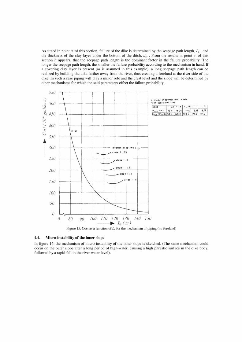
As stated in point a. of this section, failure of the dike is determined by the seepage path length, Lk , and the thickness of the clay layer under the bottom of the ditch, dks . From the results in point c. of this section it appears, that the seepage path length is the dominant factor in the failure probability. The longer the seepage path length, the smaller the failure probability according to the mechanism in hand. If a covering clay layer is present (as is assumed in this example), a long seepage path length can be realized by building the dike farther away from the river, thus creating a foreland at the river side of the dike. In such a case piping will play a minor role and the crest level and the slope will be determined by other mechanisms for which the said parameters effect the failure probability.

Figure 15. Cost as a function of Lk for the mechanism of piping (no foreland)

4.4. Micro-instability of the inner slope

In figure 16. the mechanism of micro-instability of the inner slope is sketched. (The same mechanism could occur on the outer slope after a long period of high-water, causing a high phreatic surface in the dike body, followed by a rapid fall in the river water level).

Figure 16. Mechanism of micro-instability of the inner slope

a. Failure probability

The dike is assumed to fail (collapse) if the volume of material (sand) that is transported from the inner talus to the toe of the dike is so large, that the crest of the dike is affected. As shown in figure 16 the level of point A is than at the crest level, ha .The reliability function, Z4 , that follows from this condition is: Z4 = h0 - ha ( 27 )

ha was determined according to [5]. The results of the calculations are presented in figure 17. The calculations have only been performed for the 1:2.5 and 1:3.5 slopes, the reason being that for these relatively steep slopes very low failure probabilities were found in comparison with the overtopping and piping mechanisms. Gentler slopes will lead to even lower probabilities.

Figure 17. Failure probabilities as functions of h0 for the mechanism of micro-instability of the inner slope

B-C = schematized phreatic surface during development of instability D-E = phreatic surface after development of seepage surface

h0 (m)

b. Probability density function of inundation depth The procedure to determine fd(δ) is similar to the one applied for macro-instability and for piping:

• For free flow conditions the following values for the limits of integration have been adopted: - for tb : instant at which the highest water pressure under the clay cover on the outer talus is reached (tb = 2/3 T) - te is the instant when the submerged weir situation is reached.

• For submerged weir conditions equations ( 21 ) and ( 22 ) are applicable. c. Optimum crest level

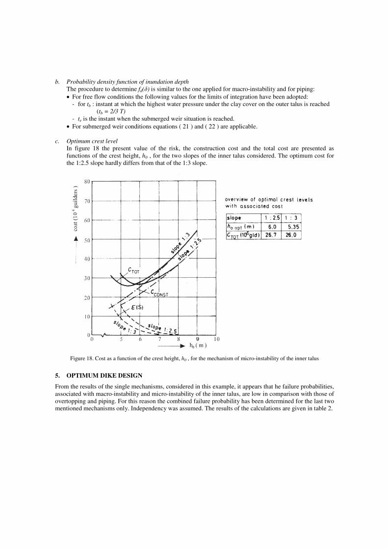
In figure 18 the present value of the risk, the construction cost and the total cost are presented as functions of the crest height, h0 , for the two slopes of the inner talus considered. The optimum cost for the 1:2.5 slope hardly differs from that of the 1:3 slope.

Figure 18. Cost as a function of the crest height, h0 , for the mechanism of micro-instability of the inner talus

5. OPTIMUM DIKE DESIGN

From the results of the single mechanisms, considered in this example, it appears that he failure probabilities, associated with macro-instability and micro-instability of the inner talus, are low in comparison with those of overtopping and piping. For this reason the combined failure probability has been determined for the last two mentioned mechanisms only. Independency was assumed. The results of the calculations are given in table 2.

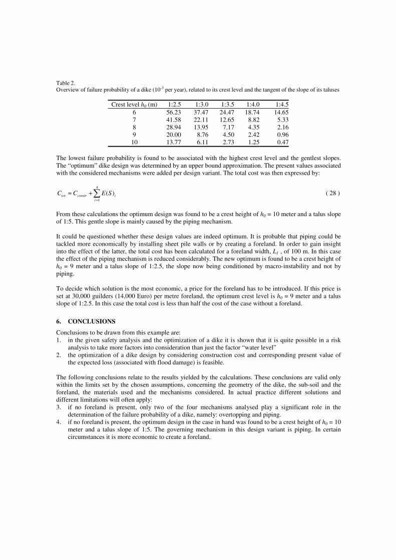
Table 2. Overview of failure probability of a dike (10-3 per year), related to its crest level and the tangent of the slope of its taluses

Crest level h0 (m) 1:2.5 1:3.0 1:3.5 1:4.0 1:4.56 56.23 37.47 24.47 18.74 14.657 41.58 22.11 12.65 8.82 5.338 28.94 13.95 7.17 4.35 2.169 20.00 8.76 4.50 2.42 0.96

10 13.77 6.11 2.73 1.25 0.47 The lowest failure probability is found to be associated with the highest crest level and the gentlest slopes. The “optimum” dike design was determined by an upper bound approximation. The present values associated with the considered mechanisms were added per design variant. The total cost was then expressed by:

4

1

( )tot constr ii

C C E S=

= +∑ ( 28 )

From these calculations the optimum design was found to be a crest height of h0 = 10 meter and a talus slope of 1:5. This gentle slope is mainly caused by the piping mechanism. It could be questioned whether these design values are indeed optimum. It is probable that piping could be tackled more economically by installing sheet pile walls or by creating a foreland. In order to gain insight into the effect of the latter, the total cost has been calculated for a foreland width, L1 , of 100 m. In this case the effect of the piping mechanism is reduced considerably. The new optimum is found to be a crest height of h0 = 9 meter and a talus slope of 1:2.5, the slope now being conditioned by macro-instability and not by piping. To decide which solution is the most economic, a price for the foreland has to be introduced. If this price is set at 30,000 guilders (14,000 Euro) per metre foreland, the optimum crest level is h0 = 9 meter and a talus slope of 1:2.5. In this case the total cost is less than half the cost of the case without a foreland.

6. CONCLUSIONS

Conclusions to be drawn from this example are: 1. in the given safety analysis and the optimization of a dike it is shown that it is quite possible in a risk

analysis to take more factors into consideration than just the factor “water level” 2. the optimization of a dike design by considering construction cost and corresponding present value of

the expected loss (associated with flood damage) is feasible. The following conclusions relate to the results yielded by the calculations. These conclusions are valid only within the limits set by the chosen assumptions, concerning the geometry of the dike, the sub-soil and the foreland, the materials used and the mechanisms considered. In actual practice different solutions and different limitations will often apply: 3. if no foreland is present, only two of the four mechanisms analysed play a significant role in the

determination of the failure probability of a dike, namely: overtopping and piping. 4. if no foreland is present, the optimum design in the case in hand was found to be a crest height of h0 = 10

meter and a talus slope of 1:5. The governing mechanism in this design variant is piping. In certain circumstances it is more economic to create a foreland.

5. in case there is a foreland a steep inner slope can be applied, as the probability of instability of the inner slope is low. The presence of a clay layer covering the outer talus is very effective with regard to water penetration into the core of the dike and to the degree of development of a high phreatic surface. For this reason the probability of instability of the inner talus (both macroinstability and micro-instability) is low in spite of the fact that a considerable permeability of the cover, due to plant roots, drying off, or the activities of burrowing animals have been taken into account.

6. restriction of the expected loss associated with the mechanisms considered can be achieved by: 1. a sufficiently high crest level h0 (limiting overtopping) 2. a clay cover on the outer slope (protecting from macro-instability and micro-instability of the inner slope) 3. the provision a foreland (as a protection against piping).

7. REFERENCES

[1] A.C.W.M. Vrouwenvelder and A.J. Wubs, “Een probabilistisch dijkontwerp”, (“A probabilistic dike design”, in Dutch), Delft, TNO B-85-64/64.3.0873, 1985.

[2] E.W. Lane, “Masonry dams on earth foundations”, Transactions ASCE, Paper 100, 1935. [3] J.B. Sellmeijer, “On the mechanism of piping under impervious structures”, Thesis TU Delft, Faculty of

Civil Engineering, 1988. [4] P.J. Visser, “Breach growth in sand-dikes”, Thesis TU Delft, Faculty of Civil Engineering and

Geosciences, 1999. [5] E.O.F. Calle, “Uitwerking grenstoestand micro-instabiliteit”, (“Limit state micro-instability”, in Dutch),

LGM note CO-263230/14, 1982. [6] S.N.Jonkman, P.H.A.J.M. van Gelder, J.K. Vrijling, Loss of life models for sea- and river floods , pages

196 - 206, Volume 1, Flood Defence, Wu et al. (eds), 2002 Science Press, New York Ltd., ISBN 1-880132-54-0.

[7] Vrijling JK, Probabilistic design of water defense systems in The Netherlands, RELIAB ENG SYST SAFE 74 (3): 337-344 DEC 2001.