reliability analysis of the electrical system in boeing ... analysis of... · reliability analysis...

Reliability Analysis of the Electrical System in Boeing 757-200

Aircraft and RB211-535 Engines

-As primary analysis for 120 minutes ETOPS approval-

Þórey Friðrikka Guðmundsdóttir

Thesis of 30 ECTS credits Master of Science (M.Sc.) in Engineering Management

June 2017





Thesis of 30 ECTS credits submitted to the School of Science and Engineering

at Reykjavík University in partial fulfillment of the requirements for the degree of

Master of Science in Engineering Management

June 2017

Supervisors:

Þorgeir Pálsson, Sc.D., Supervisor Professor, School of Science and Engineering at Reykjavík University Páll Jensson, Ph.D., Co-Supervisor

Professor, School of Science and Engineering at Reykjavík University

Examiner:

Ólafur Pétur Pálsson, Ph.D., Examiner Professor, University of Iceland

Copyright


June 2017





30 ECTS thesis submitted to the School of Science and Engineering at Reykjavík University in partial fulfillment

of the requirements for the degree of Master of Science in Engineering Management

June 2017

Student:

___________________________________________


Supervisors:

___________________________________________

Þorgeir Pálsson, Sc.D.

___________________________________________

Páll Jensson, Ph.D.

Examiner:

___________________________________________

Ólafur Pétur Pálsson, Ph.D.

The undersigned hereby grants permission to the Reykjavík University Library to reproduce

single copies of this Thesis entitled Reliability Analysis of the Electrical System in Boeing

757-200 Aircraft and RB211-535 Engines and to lend or sell such copies for private,

scholarly or scientific research purposes only.

The author reserves all other publication and other rights in association with the copyright in

the Thesis, and except as herein before provided, neither the Thesis nor any substantial portion

thereof may be printed or otherwise reproduced in any material form whatsoever without the

author’s prior written permission.

Date


Master of Science

i

ABSTRACT

Reliability Analysis of the Electrical System in Boeing 757-200 Aircraft and RB211-535

Engines

Air travel is today one of safest mode of transport. High reliability requirements have been

established in the aviation industry because of the potentially severe consequences of system

failure. In 1953, twin-engine aircraft were restricted to fly on routes that were within 60

minutes from an alternate airport. In 1985 the Extended Twin-engine Operations (ETOPS)

rules were established. They are a deviation from the 60 minute restriction, allowing twin-

engine aircraft to fly further away from an alternative airport, if operators can fulfill certain

technical and operational requirements. To obtain ETOPS approval both the aircraft and the

operator have to comply with a set of standards and regulations [1], [2].

The electrical system in Boeing 757-200 is a large and a complex system. The consequences

of losing all electrical power in-flight can cause, in worst case scenario, catastrophic accidents.

Because of the severity of such failures, a fail-safe redundancy is built into the electrical

system. The Boeing 757-200 was designed both with three and four generators. Aircrafts with

four generators have Hydraulic motor generator (HMG) added as the fourth generator. The

Boeing 757-200 aircraft with three generators is today non-ETOPS, whereas an aircraft with

four generators has ETOPS approval up to certain limits.

The main objective of this research project is to develop a quantitative method for determining

the reliability of the electrical system in Boeing 757-200 aircraft with three generators and the

reliability of the RB211-535 engines. This is done to assess whether the electrical system in

question meets the reliability requirements for 120 minutes ETOPS approval, without an

additional generator. The reliability modeling of this research project is based on the

Reliability Block Diagram technique and the commercial software tool, BlockSim 10, is used

to construct a model of the systems with the RBD approach. Analyses will be performed both

analytically and via simulation using the BlockSim software, where the software undertakes

all computations.

These results are promising and support the idea that it is a viable option to apply for a 120

minute ETOPS approval, although the electrical system only contains three generators.

Keywords: Boeing 757-200 electrical system, RB211-535 engines, Extended operation

(ETOPS) and Regulations, Reliability, Reliability Block Diagram.

ii

ÁGRIP

Áreiðanleikagreining á rafmagnskerfi í Boeing 757-200 flugvélum og RB211-535

þotuhreyflum.

Að ferðast með flugi er í dag einn af öruggustu ferðamátunum. Háar áreiðanleika kröfur hafa

fest sig í mót í flugiðnaðinum, vegna þess hversu alvarlegar afleiðingar kerfisbilanir geta haft.

Árið 1953 var tveggja hreyfla flugvélum sett sú skorða að þurfa ávallt að vera innan við 60

mínútur frá næsta flugvelli á flugleið sinni. Árið 1985 var þessi regla útvíkkuð að hluta með

tilkomu fjarflugs reglna (ETOPS reglur). Þessar reglur gefa ákveðið frávik frá 60 mínútna

skorðunni, þannig að kleyft sé að fljúga tveggja hreyfla flugvélum fjær næsta flugvelli en sem

nemur 60 mínútum, svo framralega sem rekstraraðili uppfylli ákveðnar kröfur hvað varðar

tækni og rekstur flugvéla. Til þess að öðlast ETOPS leyfi, þá þarf bæði búnaður flugélarinnar

og rekstraraðilinn að hlíta ákveðnum stöðlum og reglugerðum.

Rafmagnskerfið í Boeing 757-200 flugvélum er stórt og flókið kerfi. Afleiðing þess að missa

alla raforku á meðan flugi stendur, getur í versta mögulega tilfelli valdið hörmulegu slysi.

Vegna þess hversu alvarlegar afleiðingar slík bilun getur valdið, þá er ákveðin umfremd

innbyggð í rafmagnskerfið. Boeing 757-200 flugvélar voru á sínum tíma bæði hannaðar með

þremur og fjórum rafölum. Flugvélar með fjórum rafölum hafa vökvaknúinn rafal (HMG),

innbyggðan sem fjórða rafalinn. Boeing 757-200 flugvélar með þremur rafölum hafa í dag

ekki ETOPS leyfi, en aftur á móti þá hafa þær Boeing 757-200 flugvélar sem innihalda HMG

sem fjórða rafalinn, ETOPS leyfi upp að vissum mörkum.

Aðalmarkmið þessarar rannsóknar er að þróa megindlega aðferð til að ákvarða áreiðanleika

rafmagnskerfisins í Boeing 757-200 flugvélum með þremur rafölum og áreiðanleika RB211-

535 þotuhreyfla. Þetta er gert í þeim tilgangi að meta hvort umrætt rafmagnskerfi standist þær

áreiðanleika kröfur sem uppfylla þarf fyrir 120 mínútna ETOPS leyfi, án þess að hafa fjórða

rafalinn innbyggðan. Áreiðanleika líkanið sem þróað er í þessu rannsóknarverkefni byggir á

Áreiðanleika Blokk riti (RBD) og er BlockSim 10 hugbúnaðurinn notaður til að smíða módel

með RBD aðferðinni. Stærðfræðileg greining sem og greining með hermun er framkvæmd

með notkun BlockSim hugbúnaðarins, þar sem hugbúnaðurinn tekur yfir alla útreikninga.

Niðurstöðurnar lofa góðu og styðja við þá hugmynd að það sé raunhæfur möguleiki að sækja

um 120 mínútna ETOPS leyfi, þó svo að rafmagnskerfið innihaldi aðeins þrjá rafala.

Lykilorð: Rafmagnskerfi í Boeing 757-200, RB211-535 þotuhreyflar, ETOPS aðgerðir og

reglugerðir, Áreiðanleiki, Áreiðanleika Blokk Rit.

iii

ACKNOWLEDGEMENTS

This master thesis is the final project before receiving my master s degree in Engineering

Management at Reykjavík University. There are many that have supported me with invaluable

support and I am forever grateful to those how have helped me during the making of this

master thesis.

I would like to express my deepest gratitude to my supervisor Þorgeir Pálsson, professor at

Reykjavík University, for his endless support and motivation, for all the work and time he

made available to help me and for all his advice and guidance regarding this master thesis. I

would also like to thank Páll Jensson, professor at Reykjavík University, for all his advice and

guidance.

Special thanks go to Bragi Baldursson, head of design at Icelandair, for his strong support and

assistance by providing data and information needed for the project, for providing contacts,

setting up meeting with appropriate specialists and for all his time and work.

I would also like to thank Icelandair Technical Services (ITS), particularly Unnar

Sumarliðason, Heimir Örn Hólmarsson, Ragnheiður Guðmundsdóttir and Sveinn Haukur

Albertsson, for their support and assistant, for familiarizing me with functions and aircraft

systems needed for this master thesis.

Thanks go to Harpa Rún Garðarsdóttir and Unnur Þorleifsdóttir for all their advice and

assistance regarding this master thesis.

I would also like to thank Duane Kritzinger, author of Aircraft System Safety for his valuable

seminar and advice regarding this master thesis.

I would also like to express my gratitude to Reliasoft for their valuable seminar and support by

providing license and access to BlockSim and Weibull++. Special thanks go to Lukasz Pieniak

at Reliasoft for his assistance.

Finally, I would like to thank my parents, my fiancé Þorkell Þór Gunnarsson and my dear

daughter Elsa María Þorkelsdóttir, for there loving support, patience and for always believing

in me.


v

TABLE OF CONTENTS

ABSTRACT ..............................................................................................................................i

ÁGRIP ................................................................................................................................... ii

ACKNOWLEDGEMENTS ........................................................................................................... iii

TABLE OF CONTENTS............................................................................................................... v

TABLE OF FIGURES ................................................................................................................viii

TABLE OF TABLES................................................................................................................... x

1. INTRODUCTION ...................................................................................................................1

1.1 Background...................................................................................................................1

1.2 Statement of the problem.................................................................................................3

1.3 Aims and objectives .......................................................................................................5

1.4 Research questions .........................................................................................................7

1.5 Research contribution .....................................................................................................7

1.6 Research methodology ....................................................................................................7

1.7 Assumptions and limitations ............................................................................................8

1.8 Structure of the research project .......................................................................................9

2. INTRODUCTION TO ETOPS AND REGULATIONS....................................................................... 11

2.1 Extended operations (ETOPS)........................................................................................ 11

2.1.1 Events leading up to ETOPS .................................................................................... 12

2.1.2 Development of ETOPS .......................................................................................... 12

2.1.3 The benefits of ETOPS ........................................................................................... 15

2.2 Regulatory authorities ................................................................................................... 15

2.2.1 Requirements for 120 minutes ETOPS ...................................................................... 16

3. LITERATURE REVIEW ......................................................................................................... 17

3.1 Main definitions and terms ............................................................................................ 17

3.2 Quantitative and Qualitative Reliability Analysis. ............................................................. 18

3.2.1 Qualitative methods................................................................................................ 18

3.2.2 Quantitative methods .............................................................................................. 20

4. THEORETICAL FRAMEWORK ................................................................................................ 25

4.1 Reliability Calculations ................................................................................................. 25

vi

4.1.1 Reliability and Unreliability ..................................................................................... 25

4.1.2 Failure rate function ............................................................................................... 26

4.1.3 The Mean time to failure (MTTF)............................................................................. 27

4.1.4 The Bathtub curve .................................................................................................. 27

4.2 Life data analysis ......................................................................................................... 29

4.2.1 Life data classification ............................................................................................ 29

4.2.2 Lifetime distributions.............................................................................................. 31

4.2.3 Parameter Estimation.............................................................................................. 36

5. METHODOLOGY ................................................................................................................ 39

5.1 Reliability Block Diagrams (RBD) ................................................................................. 39

5.1.1 RBD configuration ................................................................................................. 40

5.2 Analyzing the RBD Model ............................................................................................ 46

5.2.1 Analytical analysis ................................................................................................. 46

5.2.2 Monte Carlo (MC) Simulation ................................................................................. 47

5.3 Reliability Phase Diagrams (RPD) .................................................................................. 48

5.3.1 Phase blocks.......................................................................................................... 48

5.3.2 Simulation of RPDs................................................................................................ 48

6. RELIABILITY OF THE ELECTRICAL SYSTEM IN BOEING 757-200 AIRCRAFT ................................... 51

6.1 Overview of the electrical system in Boeing 757-200 aircraft .............................................. 51

6.1.1 Difference between electrical systems with and without HMG ...................................... 53

6.2 Failure data and estimation of lifetime distributions ........................................................... 53

6.2.1 Failure models for RB211-535 Engines ..................................................................... 54

6.2.2 Failure models for IDGs.......................................................................................... 56

6.2.3 Failure models for APU generator ............................................................................ 57

6.2.4 Failure model for HMG .......................................................................................... 58

6.2.5 Data concerning APU start in-flight. ......................................................................... 59

6.3 System reliability models .............................................................................................. 59

6.3.1 RBD for the engines ............................................................................................... 60

6.3.2 RBD of a system without HMG................................................................................ 60

6.3.3 RBD of a system with HMG .................................................................................... 63

6.4 Reliability Phase Diagram (RPD) ................................................................................... 66

vii

6.4.1 The RPD model ..................................................................................................... 68

7. RESULTS AND DISCUSSIONS................................................................................................ 71

7.1 In-flight start of APU .................................................................................................... 72

7.2 IFSD rate .................................................................................................................... 72

7.3 Engines ...................................................................................................................... 73

7.3.1 Analytical calculations ............................................................................................ 73

7.3.2 Simulation ............................................................................................................ 74

7.4 Results from reliability analysis using stand-by container. .................................................. 78

7.4.1 System without an HMG ......................................................................................... 78

7.4.2 System with an HMG ............................................................................................. 83

7.4.3 Comparison of results for a systems with and without HMG ......................................... 85

7.5 Diversion due to different failure modes .......................................................................... 86

7.5.1 Diversion due to a single engine failure ..................................................................... 87

7.5.2 Diversion due to a dual generator failure (IDG and APU generator) ............................... 91

7.5.3 Comparison and discussion...................................................................................... 94

7.6 Simulation by using RPD approach ................................................................................. 96

7.6.1 System without an HMG ......................................................................................... 96

7.6.2 System with an HMG ............................................................................................. 98

7.7 Suitability of selected methods and software .................................................................... 99

8. SUMMARY AND CONCLUSIONS .......................................................................................... 101

8.1 Summary .................................................................................................................. 101

8.2 Conclusions .............................................................................................................. 102

8.3 Future work............................................................................................................... 105

9. REFERENCES ................................................................................................................... 107

10. APPENDIXES ................................................................................................................. 111

A. Maintainability and Availability .................................................................................... 111

B. Lifetime distributions .................................................................................................. 113

B.1 The Normal Distribution ......................................................................................... 113

B.2 The Lognormal Distribution .................................................................................... 115

C. 757-200 Electrical block diagram with an HMG............................................................... 119

D. 757-200 Electrical Block Diagram without an HMG......................................................... 120

viii

TABLE OF FIGURES Figure 1-1: Icelandair´s route network [3] ...................................................................................1

Figure 2-1: Routes for a flight from London (LHR) to New York (JFK) under both 60 and 120 minute

ETOPS rules [22]. .................................................................................................................. 13

Figure 4-1: Relationship between reliability and unreliability [43]................................................. 26

Figure 4-2: The "Bathtub curve" showing three life stages of failure rate vs. time [45]..................... 28

Figure 4-3: Example of complete data sample set [37]. ............................................................... 30

Figure 4-4: Example of data set with suspension [37]. ................................................................ 30

Figure 4-5: Example of Interval censored data [37]..................................................................... 30

Figure 4-6: Example data set with left censoring [37] ................................................................. 31

Figure 4-7: Exponential pdf with two different values of the failure rate λ [40]. .............................. 32

Figure 4-8: Weibull pdf with three different values of the shape parameter β [40]. ......................... 34

Figure 4-9: Weibull failure rate with three different values of the shape parameter β [40]. .............. 34

Figure 4-10: Weibull pdf with three different values of η [40]. ..................................................... 35

Figure 5-1: Example of Reliability Block Diagram [55]. ................................................................ 40

Figure 5-2: Example of a series structured system [14]. .............................................................. 41

Figure 5-3: Example of a parallel structured system [14]. ............................................................ 42

Figure 5-4: Example of k-out-of-n structure [56]. ....................................................................... 43

Figure 5-5: Example of blocks in a load sharing container [14]. .................................................... 44

Figure 5-6: Example of blocks in a standby container [15]. .......................................................... 45

Figure 6-1: Electrical System Overview [64]............................................................................... 52

Figure 6-2: RBD model of engines............................................................................................ 60

Figure 6-3: RBD model of engines and generators in stand-by container ....................................... 61

Figure 6-4: RBD model of the system in normal phase ................................................................ 62

Figure 6-5: RBD of the system in diversion phase ....................................................................... 63

Figure 6-6: RBD model of engines and generators with HMG in Standby container ......................... 64

Figure 6-7: RBD model of the system with HMG in normal phase ................................................. 65

Figure 6-8: RBD of the system with HMG in diversion phase ........................................................ 65

Figure 6-9: Route form Keflavik to Seattle - Non ETOPS [62] ........................................................ 67

Figure 6-10: Route from Keflavik to Seattle - 120 minutes ETOPS approval [62] ............................. 67

Figure 6-11: RPD used to simulate systems ............................................................................... 68

Figure 7-1: Data on APU In-flight start, represented on a 12-month rolling average base. ................ 72

Figure 7-2: Frequency of single engine failures in each phase, results from simulating the RPD........ 77

Figure 7-3: Reliability function; system with three generators where two active paths are required. . 80

Figure 7-4: Reliability function; system with three generators where one active path is required. ..... 81

Figure 7-5: Reliability function; system with four generators where one active path is required........ 84

Figure 7-6: Reliability functions; both systems where one generator is required as a minimum........ 86

ix

Figure 7-7: Frequency of failures in each phase for a system without an HMG............................... 97

Figure 7-8: Frequency of failures in each phase for a system with an HMG. ................................... 99

Figure B-1: Normal pdf with three different values of σ [61]. ..................................................... 114

Figure B-2: Normal failure rate with three different values of σ [61]. .......................................... 114

Figure B-3: Lognormal pdf with two different values of u'[37].................................................... 116

Figure B-4: Lognormal pdf with two different values of σ' [37] ................................................... 116

Figure B-5: Lognormal failure rate with three different values of σ' [64]. ..................................... 117

x

TABLE OF TABLES

1

1. INTRODUCTION

This chapter will provide the reader with a general introduction of this research project. First

the background and statement of the problem, as well as aims and objectives are introduced.

Research questions, contribution, assumptions and limitations are then listed, along with a

short description of the research methodology. Finally the structure of this master thesis is

presented.

1.1 Background

Icelandair is the main airline in Iceland with roots dating back to 1937. It has been growing

significantly over the last decade. In 2015 the airline carried for the first time more than three

million passengers, in 2016 they carried 3.7 million passangers and are predicting to pass the

four million mark in 2017. Iceland’s geographical location, between Europe and North

America, plays a key role in Icelandair´s route network. This route network with Iceland

serving as a hub, allows Icelandair to offer flights to and from Iceland as well as connections

between multiple cities for passengers travelling across the North Atlantic. Thus today’s route

network, which can be seen in figure 1-1, connects 27 European airports with 16 North

American airports [3], [4].

Figure 1-1: Icelandair´s route network [3]

2

Icelandair is the largest Boeing 757 operator in Europe, their fleet consists of 28 Boeing 757-

200 and one 757-300 narrow-body aircraft, along with two Boeing 767 wide-body aircraft.

Since 1953, twin-engine aircraft, such as Boeing 757 which Icelandair operates, have been

restricted to fly on a route that is within 60 minutes from an alternate airport1 at a one-engine

inoperative cruise speed2. The Extended Twin-engine Operations (ETOPS) rules3, which are a

deviation from the 60 minute restriction, were established in 1985 as a response to rapid

technological evolution when very economical long-range twin engine aircraft came on the

market. Virtually every system in the aircraft and in particular the turbine engines had

undergone enormous changes in the reliability. In the beginning the ETOPS abbreviation

stood for “Extended twin-engine operations” and was therefore limited to aircraft with only

two engines. But with the newest update of the ETOPS regulation, the abbreviation has now

been redefined to mean “Extended operations”, restricting all passenger-carrying aircrafts

whether they are two, three or four-engine aircraft [2],[6],[1]. They are however restricted in

different ways depending on the number of engines (see chapter 2). All aircrafts may need to

divert4 for some reason, such as passenger illness, turbulence, fuel leaks, cargo fire, significant

system5 failure or an engine failure. The whole ETOPS concept is to preclude such diversions

and, if they were to occur, to have programs in place to protect the diversion. ETOPS is a

conservative, evolutionary program that enhances safety, reliability, and efficiency during

extended operations [2].

From reference such as [2] the preclude and protect concept is explained further;

Preclude – “ETOPS design enhancements have increased the robustness of airplane systems

and driven further gains in the extreme reliability of modern fanjet engines. ETOPS

maintenance requirements also reduce diversions through engine condition and oil

level/consumption monitoring, the aggressive resolution of reliability issues, and procedures

to avoid human error during maintenance of airplane engines and systems.”

Protect – “ETOPS protects diverting jetliners through safety-enhancing operational

requirements such as dispatch, communications, alternate airport weather and fuel.”

The reliability of technical components and systems, i.e. hardware reliability, is a concept that

has been applied for a very long time, starting just after World War I [7]. Reliability analyses

are applicable in many areas and there exists a vast literature on reliability. Reliability analysis

1 An alternate airport is an airport that satisfies all requirements and regulations concerning an ETOPS flights, such as [5]. Operators must present a l ist of alternate airports for a specific area of operation to the local operational authorities as a part of the operational approval [1], [5]. 2 The one-engine-inoperative cruise speed for the intended area of operation must be a speed, within the certificated limits of the aircraft, selected by the operator and approved by the competent authority [5]. 3 See more extensive coverage of ETOPS rules and ETOPS evolution in chapter 2. 4 When a fl ight is diverted, the fl ight has been routed to an airport other than its intended destination [2]. 5 Aircraft propulsion system or any other system whose failure could adversely affect the safety of the fl ight[5].

3

is extremely important in some fields, where the tolerance for failure must be close to zero.

Failures in complex systems such as nuclear power plants and aircraft propulsion systems can

be disastrous, thus the requirements on reliability in such systems is very high [8].

Air transport is one of the fastest growing modes of transport [9]. In 2015 the total number of

airline passengers increased by 6,4 % and is projected to continue to grow at an annual rate

of 5 % to 6 % over the next years because of the ongoing growth in air transport demand [9],

[10]. Air travel is today one of safest mode of transport. High reliability requirements have

been established in the aviation industry because of the potentially severe consequences of

system failure. Thus safety is one of the main driving forces within civil aviation [8]. Because

failure of significant systems in aircraft can adversely affect the safety of a flight, fail-safe

redundancy is built into the systems, e.g. hydraulic and electrical system, to increase

reliability. So if for example one generator fails, the safety of the aircraft is not jeopardized,

although the aircraft might have to divert to the nearest available airport.

Electrical power sources, i.e. jet engines and Auxiliary Power Units (APU), and associated

generators, e.g. two integrated drive generators (IDG) and one APU generator, are an example

of a redundant system with increased dependability and reliability over a non-redundant

system. Developing a quantitative reliability model of the electrical power sources and

associated generators can however be a difficult task. Quantitative reliability model of such

systems can benefit operators, not only by giving the estimate of the reliability, but also by

being a tool that can be used for the purpose of analyzing, for example, different maintenance

strategies and the effect of failure characteristics of different types of components on the

overall system.

1.2 Statement of the problem

Of the 28 Boeing 757-200 operated by Icelandair 18 have ETOPS approval for flying at a

distance of up to 180 minutes from an alternate airport. To obtain such an approval the aircraft

itself must first receive a type design approval, called type certificate (TC), which is issued by

the relevant aviation regulatory authorities and signifies the airworthiness6 of the aircraft

design and manufacture. The second step is to obtain operational approval from the relevant

aviation regulation authorities. Operators pursuing to obtain ETOPS approval have to fulfill

stringent requirements regarding maintenance, operations, training and reliability programs

[2], [1] in addition to potential improvements to aircraft systems and/or components.

When an aircraft has obtained a type design certificate, the design of the aircraft cannot be

changed. If a manufacturer or an operator wants to modify the aircraft from its original design

they need to apply for a Supplemental Type Certificate (STC). There are many steps involved

6 Airworthiness is a measure of an aircraft´s condition and suitability for safe fl ight [11].

4

in the STC approval process, which often include extensive technical analysis and in-depth

regulatory review [5], [12].

Icelandair is seeking to get a 120 minutes ETOPS approval for the 10 remaining Boeing 757-

200 twinjets. As for now these aircraft are non-ETOPS and therefore restricted to fly on routes

that do not go further than 60 minutes from an alternate airport at a one-engine inoperative

cruise speed. However there is a difference in the original design of these aircraft, i.e. the 18

Boeing 757-200 with approved 180 minutes ETOPS and the 10 Boeing 757-200 that do not

have ETOPS approval. Those that are already approved have four independent electrical

power sources. Primary power is supplied by two engine-driven (RB211-535 engines)

integrated drive generators (IDG). The third power source is an Auxiliary power unit (APU)-

driven generator, which provides an in-flight back-up for the two main engine-driven IDG.

The fourth power source is a Hydraulic motor generator (HMG) which is automatically

activated if all alternating current (AC) power is lost during flight. Those aircraft that are non-

ETOPS only have three independent electrical power sources as the original design does not

include an installation of an HMG.

Despite the fact that regulations, published by EASA [5] and by FAA [6], only require three

independent electrical power sources for ETOPS approval up to 180 minutes, the

airframe/engine combination of Boeing 757-200 aircrafts that have obtained a type design

approval for ETOPS all have four independent electrical power sources. The reason for this

can most likely be attributed to the fact that when the Boeing 757-200 airframe/engine

combination received ETOPS type design approval in 1986 the reliability of the propulsion

system, electrical system and other critical systems were not as high as it is today. Therefore

there may have been a valid reason for requiring a standby electrical power source like the

HMG. In order to obtain an ETOPS approval for up to 120 minutes limit for the remaining 10

Boeing 757-200, the airline either must have each aircraft modified by the manufacturer, i.e.

installation of the HMG by Boeing or other approved maintenance organization, or seek

approval for a new STC from the relevant aviation authorities, i.e. EASA. To be eligible for

120 minute ETOPS Icelandair has to fulfill stringent requirements, such as are spelled out in

the EASA regulations. The airline must demonstrate that all specified reliability requirements

are fulfilled regarding critical systems, such as propulsion and electrical systems, and that all

operational requirements are satisfied [2], [5].

In this research project a quantitative reliability model will be structured to calculate the

reliability of the system, i.e. three independent power sources (two engines and APU) and

three dependent generators (two IDGs and one APU generator), in order to demonstrate that

all requirements regarding reliability are met, despite having only three power sources.

5

The requirements related to this research project are according to [5] the following;

In-flight start reliability of the APU 7 should not be less than 95%.

In-flight shut-down (IFSD) rate needs to be equal to or less than 0.027 shutdowns per

1000 engine flight hours.

The probability of a catastrophic accident due to complete loss of thrust from

independent causes must be no worse than 0.3 x 10-8 per flying hour.

In addition to these requirements, which are listed in AMC 20-6, Icelandair wants to

demonstrate that the probability of losing two out of three electrical power sources meets the

safety objective of being less than or on the order of 10-5 per flying hour. Which is defined as

probability of a major failure condition according to the Certification Specifications for Large

Aeroplanes (CS-25) and can be found in reference such as [13].

Extensive and more detailed coverage regarding regulations for both ETOPS type design

approval and ETOPS operational approval can be found in references, such as [5] ,[6] and

[13]. Whereas Icelandair already has obtained an ETOPS operational approval for 180

minutes, there is no need to apply for a new one. However some additional in-flight

maintenance actions or procedures or training might need to be implemented.

Developing a quantitative reliability model to estimate the system reliability is beneficial for

Icelandair for a number of reasons. Not only can it be used to assess if current non-ETOPS

engine/airframe combination meets established requirements for 120 minutes ETOPS. It can

also be used to identify the weakest link in the system and to plan maintenance actions to

increase reliability and/or reduce cost associated with maintenance strategies.

1.3 Aims and objectives

The main objective of this research project is to develop a quantitative method for determining

the reliability of a system consisting of three power sources (two engines and an APU) and the

three associated electrical generators of the Boeing 757-200 aircraft operated by Icelandair.

The objective is also to assess whether the electrical system in question meets the reliability

requirements for 120 minutes ETOPS approval, i.e. whether they fulfill requirements to extend

the permitted flying time from the nearest alternate airport from 60 minutes to 120 minutes,

without an additional generator. The objective is also to compare the reliability of an electrical

system containing four generators (HMG as the fourth) with 180 minutes ETOPS approval

7 The APU is usually not running in air unless a failure, causing engines or main generators to fail, has occurred. It is a backup system, which can be started in flight if needed. The In-flight start of the APU must be at 95% or above to fulfill ETOPS requirements.

6

with an electrical system consisting of three generators (without an HMG) with a diversion

time of 120 minutes.

The quantitative method that will be developed for determining the reliability of the system

will be based on a recognized modeling technique that provides a description of how various

components interact reliability-wise to deliver the designed functionality of the overall system.

Critical components in the primary alternating current (AC) electrical power system will be

modeled, reflecting their reliability-wise connection. The resulting reliability model should

then enable calculations of the systems overall reliability. In order to achieve the aim and

objectives of this research project, the following tasks will be performed:

Initial analysis of the primary AC power system, which will lead up to a model of all

critical components in the system.

Data collection. Data will be collected from both manufacturers and other airlines that

operate Boeing 757-200, with the same airframe and engine combination as Icelandair

operates.

Data analysis to assess whether IFSD rate and In-flight start reliability of APU meet

the requirements that need to be fulfilled.

Survey of what methods have previously been used to determine the reliability of

primary AC power system in aircraft, the propulsion system or similar systems. A

survey of this type would be useful in evaluating which method is likely to answer the

questions of this research project.

Develop a sub-model that consists only of engines, to calculate the reliability and

probability of dual engine failure.

Develop a reliability model of all electrical power sources (engines and APU) and

associated generators to calculate the reliability and probability of losing AC power.

Develop a system reliability model with a fourth power generator installed, namely the

HMG, and comparing this to reliability model with three power generators with

varying diversion times.

Perform analytical calculations, on each of these models, using suitable software to

determine the reliability of each system.

Perform a simulation, using suitable software to examine the behavior of the systems

and determine reliability metrics of interest.

Provide reliability results that can be used to assess whether it is viable to apply for

120 minutes ETOPS approval without the installation of an HMG.

7

1.4 Research questions

While analyzing the reliability of the system, i.e. electrical power sources (engines and APU),

IDG and APU generators the following research questions will be answered:

1. What is the overall reliability of the electrical system in question?

2. Are all requirements listed in chapter 1.2, fulfilled for a system without an HMG?

3. What is the probability of failure of a system with three generators with maximum

diversion time of 120 minutes compared to a system with HMG installed as the fourth

generator with approved maximum diversion time of 180 minutes? Is there a

significant difference?

4. Is it suitable and convenient to use the selected method to construct a model which is

comprised of RB-211 jet engines and electrical system with either three or four

generators?

5. Is it suitable and convenient to use the selected method and software to analyze and

determine the reliability of the systems?

6. What further research and development work needs to be done as extension of this

research project?

These questions will be answered and discussed in detailed in chapter 7 and 8.

1.5 Research contribution

The main contributions of this research project are expected to be the following:

Formal initial analysis of the reliability of the primary AC power system in Boeing

757-200 aircraft.

Formal analysis of requirements and regulations that need to be fulfilled.

Assessment of methods that could be eligible for determining the reliability of the

system.

Large database, where data is collected from other airlines and manufactures. Data can

be used to compare reliability of components between operators.

A reliability results that confirms whether requirements and regulations considered in

this research project are meet.

A reliability model that could be used for further studies.

1.6 Research methodology

Multiple approaches are available for modeling and analyzing system reliability. As systems

get more complex and modeling requires a more detail description of the real-life systems,

8

with for example maintenance actions, many approaches may not be considered fit for

analyzing the systems. Therefore a survey of different methods that are often used for

analyzing systems reliability is presented in chapter 3. The methods that were considered most

fitting for this research project were life data analysis to analyze real-life data from Icelandair

and other operators and Reliability Block Diagram (RBD) for modeling the system, being

analyzed. Both analytical approaches and Monte Carlo (MC) simulation were used to analyze

the RBD model. These methods are described in more detail in chapters 4 and 5.

The Weibull++ software tool, developed by Reliasoft Corporation will be used to analyze the

data gathered from operators and to obtain a failure distribution for each component. The

commercial software tool, BlockSim 10, also developed and published by Reliasoft

Corporation will be used to model the system. The BlockSim software offers a sophisticated

graphical interface that enable modelling of both simple and extremely complex systems using

RBD or Fault Tree analysis (FTA). Calculations through BlockSim on overall system

reliability can be performed analytically or with MC simulation. In this research project the

software will be used to simulate the model and to perform analytical analysis.

1.7 Assumptions and limitations

The electrical system in the Boeing 757-200 aircraft is large, highly complex system, which

contains various interacting sub-systems. The focus in this research project will be on the main

components in the electrical system, i.e. engines, IDGs, APU generator, in-flight start on APU

and HMG. These are the critical components in the system and each of them will be presented

with a single block in the model. The reason for not breaking those components further down

is because only severe failures that cause complete loss are being considered. Furthermore

data collecting would be difficult, where such detailed data is usually not available. All results

are therefore limited to failures causing either total engine shutdown or a generator shutdown.

Separate models will be built, model for a system with an HMG installed as the fourth

generator and a model for a system without an HMG. Systems are modeled in their present

configuration when determining their reliability.

Data on complete failures (or shut down) of engines and generators will be collected, without

considering the underlying causes. It is assumed that components fail independently of other

components. The system is analyzed over one flight including the possibility of a diversion.

Furthermore it is assumed that the system is in “as good as new” condition before each flight.

Therefore routine maintenance and inspection actions will not be included directly. This is

done because the failures that are being analyzed are so severe that in most cases they cannot

be repaired with routine maintenance action. It is assumed that normal line maintenance

actions and other on-wing maintenance actions are carried out to maintain the health of the

9

engine and generators. The system is therefore thought of as non-repairable when analyzing it

because we assume that all maintenance actions are reflected in the data.

It was not possible to obtain failure data on HMG. The reason for this is that the HMG is so

rarely used in-flight that no operational failure data exists to the knowledge of Icelandair

personnel. It is assumed that the HMG would have similar failure distribution as the APU

generator. It is also assumed that the HMG has a perfict start, i.e. if needed it will always start

successfully. The assumption is also made that if the APU starts, the APU itself will not fail. It

is therefore presented as a single component that will either start or not with certain

probabilities. This limits the results as reliability results are only as accurate as the data

available for the components in the system.

It is assumed that components, when in dormant mode, cannot fail. This assumption is made

for both systems, i.e. with and without an HMG and may cause the system to be slightly more

reliable. Due to the fact that this assumption is made for both systems, this should not have

decisive effect on the overall reliability results.

In the analytical analysis, the reliability and other matrices of interest are calculated over a

predefined period. It is also assumed that a maximum allowable diversion time is needed, two

hours for a system without HMG and three hours for a system with HMG.

In the simulation, the hours for each phase in the model are assumed to be fixed throughout all

simulations. No maintenance actions or inspections are performed as the system is assumed to

be non-reparable. It is also assumed that the stress loads between different phases, e.g. stress

load on components form take-off to landing, is the same in all phases.

Other assumptions made, regarding specific components and selection of failure distributions

for each component will be stated in the appropriate chapters.

1.8 Structure of the research project

Chapter 1 presents the motivation for undertaking this research project and provides the

objectives, methodology and research questions that apply in this work. Chapter 2 provides the

reader with information on the concept of extended twin operations or ETOPS, why these are

important for an airline and what requirements are associated for the approval of ETOPS

regarding propulsion system and electrical system. In chapter 3 commonly used methods when

performing reliability analysis are introduced along with an explanation on basic terms used in

this research project. Chapter 4 is intended to provide the reader with general information

about reliability theory, life data analysis and the mathematics behind these subjects. In

chapter 5 the RBD methodology used in this research project is explained in detail. Chapter 6

presents the in-depth study of the electrical power system and associated generators and

10

equipment. The results and discussions of the reliability analysis are presented in chapter 7

and finally conclusions and summary of this Master thesis is presented in chapter 8.

11

2. INTRODUCTION TO ETOPS AND REGULATIONS

This chapter is intended to provide the reader with an overview of the concept of ETOPS,

events leading up to the establishment of the ETOPS rules, how the rules have developed over

time and what benefits are gained from their adoption in airline operations.

2.1 Extended operations (ETOPS)

Since 1953, twin-engine aircraft have been restricted to fly on routes that are always within 60

minutes from an alternate airport flying at a single-engine operative cruise speed, approved by

the appropriate authorities. ETOPS stands for “Extended operations” and is an abbreviation

created by the International Civil Aviation Organization (ICAO) to describe deviations from

the 60 minute restriction. The ETOPS rules were established as a response to rapid

technological evolution concerning virtually every system in the aircraft and the engine as

well. With the development and advent of new technology the reliability of aircraft systems

and engines had increased enormously. Consequently the Federal Aviation Administration

(FAA) and other major Civil Aviation Authorities8 (CAA) estimated that it was safe for twin-

engine aircraft to exceed the 60-minute operating restriction if operators could fulfill certain

technical and operational requirements. Since ETOPS flying began in 1985, millions of

ETOPS flights have been flown. Today there are over 143 operators worldwide flying about

1700 ETOPS flights every day [2],[1].

In the beginning the ETOPS abbreviation stood for “Extended twin-engine operations” and

was therefore limited to aircraft with only two engines. But with the latest update of the

ETOPS regulation, the abbreviation has now been redefined to mean “Extended operations”,

imposing constraints on all passenger-carrying aircraft whether they are two, three or four-

engine aircraft [2],[6],[1]. However the limits are different for twin-engine aircraft than for

three-and four-engine aircrafts.

To obtain ETOPS approval both the aircraft and the operator (airline) have to comply with a

set of standards. The approval is a two-step process. First step is the aircraft type design

approval, where the aircraft model type, airframe/engine combination, must be approved for

extended operations. The second step is to obtain operational approval from relevant aviation

regulation authorities. Operators pursuing to obtain ETOPS approval have to fulfill stringent

requirements regarding maintenance, operations, training and reliability programs [1], [2].

8 ETOPS requirements are essentially the same for all the Aviation authorities [1]. Aviation authorities

in Europe, like European Aviation Safety Agency (EASA) has incorporated similar requirements as FAA

have in the United States.

12

The ETOPS rules are designed to eliminate as much risk as reasonably possible to ensure a

safe flight. The ETOPS rules provide a very high level of safety while enabling the use of

twin-engine aircrafts on routes which were previously open to three- and four-engine aircraft

only. The farther an operator wants to fly from an alternate airport, the more stringent

requirements have to be fulfilled, to minimize risk [1], [6].

“If it weren’t for ETOPS, airlines and the traveling public would not have been able to benefit

from the leading safety, reliability, and efficiency of long-range twinjets on extended-

diversion-time air routes. The reason is a longstanding operating restriction on two-engine

airliners that is informally known as the 60-minute rule”[2]

2.1.1 Events leading up to ETOPS

The first non-stop transatlantic9 flight was carried out in the year 1919, when two British

aviators, John Alcock and Lieutenant Arthur Whitten Brown, flew over the Atlantic Ocean in

a Vickers Vimy aircraft10. They flew from Canada to Ireland and the flight took just over

sixteen hours [16]. In 1936 the U.S. established a rule that prohibited all types of aircraft,

regardless of the number of engines, to fly more than 100 miles from an alternate airport in

commercial transport operations. In 1953, as a response to limited reliability of combustion

engines, such as the piston engines that powered most aircrafts in the 1940s and early 1950s,

the U.S. Federal Aviation Administration established the 60-minute rule in 1953. The 60-

minute rule focused on engine reliability, it involved restricting two-engine aircraft to routes

that remain within 60 minutes from an alternate airport, at one engine inoperative cruise speed.

The intention of the 60 minutes rule was to reduce the risk of a catastrophic accident by

restricting aircraft to be within an acceptable distance from the nearest airport that is adequate

for landing in the event of an emergency. If one engine failed at any point along the route a

safe landing could be made before the remaining engine would fail. Although this rule was

intended for two-engine aircrafts, it was also applied to three-engine aircrafts in the beginning

[2], [1], [6]. Since the 60-minute rule was established major developments in flight-related

technologies has improved the reliability of nearly every system in the aircraft. The aviation

industry also converted to turbine propulsion that lead to major improvements in engine

reliability [1], [17]. Because of this rapid growth in engine reliability, FAA changed the 60-

minute rule in 1964, so that three-engine, turbine-powered aircrafts would be exempted from

the rule. After that only twin-engine operators were restricted by the rule [2], [6].

2.1.2 Development of ETOPS

Over the next decades further advancements in airframe, avionics, and propulsion system

technology was achieved and with the advent of high-bypass-ratio turbofan engines, an 9 A Flight which spans over the Atlantic Ocean is a transatlantic flight [14]. 10 Vickers Vimy was a British aircraft, originally designed as a heavy bomber for England in World War I [15].

13

enormous progress was made in the engine efficiency and overall reliability of civil aircrafts.

With this technological progress, twin-engine aircrafts or twinjets could be designed with the

performance and safety improvements that enable them to fly safely on routes beyond 60

minutes from alternate airport. Thus with time, the 60-minute rule needed reconsideration. In

the early 1980s ICAO started to examine the possibility of twinjets operating beyond the 60

minute operating restriction. Criteria’s (both from design and operational point of view) that

needed to be met to ensure a very high level of reliability were identified and defined. The

results were the ETOPS program, which was established for the ETOPS approval of new

aircrafts as well as relaxation of the 60 min rule for aircrafts already in operation [2], [1].

In 1985, the FAA published Advisory Circular (AC) 120-42, also known as the 120-minute

ETOPS rule. ACs are intended to provide institutions and individuals within the aviation

industry, information and guidance. AC 120-42 provided guidance on how to comply with

Federal Aviation Regulations11 (FAR) by defining an acceptable means of compliance in order

to get permission to exceed the 60-minute operating restriction. By fulfilling all the 120-

minute ETOPS rule s stringent requirements, operators were permitted to fly their twinjets on

routes that remained within 120 minutes at all points from an alternate airport [2], [6].

Figure 2-1: Routes for a flight from London (LHR) to New York (JFK) under both 60 and 120 minute ETOPS rules [22].

In Figure 2-1, the difference between 60 and 120 minutes ETOPS routes from London to New

York can be seen. If a twinjet and its operator are not certified for 120 min ETOPS operations

it cannot fly the route represented by the straight white line from London to New York, it

would have to stay within the blue circular area.

11 Federal Aviation Regulations (FAR) are mandates for controlling all aspects of aviation in the U.S. The Federal Aviation Administration (FAA) establishes these regulations [18].

14

In 1988, FAA published AC 120-42A, also known as 180 minute ETOPS rule. This permitted

operators fulfilling all requirements to fly their twinjets on routes that remain within 180

minutes from alternate airport [2].

From the time that the ETOPS rules were established in 1985, they have been constantly

evolving. The latest update appeared in 2007 when the FAA published AC 120-42B. With this

new update, the legal definition of ETOPS was changed. Now the rule did not only restrict

twinjets, but also affected three-and four-engine aircrafts that carried passengers [2], [6].

“Currently, engine reliability has improved to a level where the safety of the operations is not

impacted so much by the number of engines, but by other factors that affect operations of all

airplanes whose routings take them great distances from adequate airports [6].”

“Operational data shows that the diversion rate for all airplane-related and non-airplane related

causes are comparable between two-engine airplanes and airplanes with more than two engines.

Consequently, the FAA has found that there is a need for all passenger carrying operations

beyond 180 minutes from an adequate airport to adopt many of the ETOPS requirements that have

been based on sound safety principles and successfully proven over many years of operations.”

So from the update in 2007 the abbreviation ETOPS has stood for Extended Operations

instead of Extended Twin-Engine Operations. However, there is a difference in when the

ETOPS rules apply, i.e. the definition of when the aircraft has reached a distance that would

be classified as an extended operation is different between two-engine and three-and four-

engine aircrafts. For twinjets the ETOPS rule still applies if it flies on a route that at some

point goes further than 60 minutes from an alternate airport. However for three-and four-

engine passenger carrying aircrafts, the ETOPS rule applies when they fly on routes that at

some point goes further than 180 minutes from an alternate airport [2], [6].

Today there are many deviations from the original ETOPS rule. According to AC-120-42B,

operators that fulfill all relevant ETOPS requirements can apply for ETOPS certification in

any of the following categories [6];

75-minute ETOPS

90-minute ETOPS

120-minute ETOPS

138-minute ETOPS

180-minute ETOPS

207-minute ETOPS (in the North Pacific Area of Operation)

240-minute ETOPS (approvals are based on specific geographical areas)

Beyond 240-minute ETOPS (approvals at this level are based on particular city pairs)

15

2.1.3 The benefits of ETOPS

Before the ETOPS rules were established, three-and four-engine aircraft served the majority of

all long-haul routes. With the advent of ETOPS two-engine aircraft now account for the

majority of these flights [2]. The benefits of ETOPS flights are multiple both for operators and

passengers as well. In figure 2-1, the efficiency of flying direct ETOPS flight, on a route that

permits 120 minutes instead of 60 minutes from a suitable alternate airport, can be

demonstrated by comparing the distance, time and fuel savings between those routes [1]. For

passengers, ETOPS, for example, provides benefits through a greater variety of flights to

choose from with different departures. There is also a potential for lower ticket price because

operational costs per seat-mile associated with two-engine aircrafts is likely to be less than for

three-and four-engine aircrafts. For operators, ETOPS benefits are derived through increased

operational flexibility, more direct routings, increased passenger satisfaction, greater

profitability and efficiency. More importantly, ETOPS has benefited both operators and

passengers by making aviation safer [2],[1].

2.2 Regulatory authorities

The FAA is the national aviation authority of the United States. The European Aviation Safety

Agency (EASA) is an agency of the European Union (EU) and hence the European aviation

authority. Countries that are a part of the European Economic Area (EEA) as well as

Switzerland are also members of EASA. The mission of both these agencies is, among other

things, to implement the highest common standards of safety and environmental protection in

civil aviation [19], [20].

Acceptable Means of Compliance (AMC) 20-6 is a document published by EASA. AMC 20-6

describes the means to establish compliance with the basic regulations and implementing

rules published by EASA [6], [5]. EASA has adopted similar requirements as the FAA

regarding ETOPS rules, so essentially the rules and requirements should be the same [2].

A newly developed aircraft model must obtain a type certificate from relevant aviation

regulatory authorities, before the aircraft may start operation. FAA and EASA are the main

agencies world-wide responsible for the certification of aircraft [2]. To obtain ETOPS

approval both the aircraft and the operator (airline) have to comply with a set of standards.

The Approval is a two-step process [6];

1. Type design approval of aircraft and engine combination

2. Operational approval

Certificate holders must demonstrate that the operation can be conducted at a level of

reliability that achieves and maintains an acceptable level of risk as defined by the

16

requirements. Permission is granted as long as adequate safety is demonstrated and current

levels of safety maintained [6].

2.2.1 Requirements for 120 minutes ETOPS

In this research project the main focus is on requirements concerning the reliability of the

propulsion system and primary AC electrical power system. For that reason, not all

requirements and rules need for ETOPS approval are being considered, only those relating to

this research project concerning the propulsion and electrical system.

The requirements related to this research project are according to [5] the following;

In-flight start reliability of the APU should not be less than 95%.

In-flight shut-down (IFSD) rate needs to be equal to or less than 0.027 shutdowns per

1000 engine flight hours.






probability of a major failure condition in Certifications Specifications for Large Aeroplanes

(CS-25) [13].

Extensive and more detailed coverage regarding regulations for both ETOPS type design

approval and ETOPS operational approval can be found in references such as [5], [6] and [13].

17

3. LITERATURE REVIEW

The purpose of this chapter is to provide an overview of the main definitions and terms in

reliability theory that are used in this research project. Also to give a short description of

commonly used methods in reliability and their associated literature from the aviation

industry.

3.1 Main definitions and terms

Reliability is defined as the probability that a component or system will perform its required

function under stated conditions for a specific period of time [7], [21].

Unreliability is the inverse of reliability. It is the probability of a component or system failure

over a specific period of time [7], [22].

Non-Repairable systems are systems that cannot be or do not get repairers after failures. The

components are not repaired or replace when a failure occurs [22]. No maintenance actions are

therefor considered. When calculating the reliability for non-repairable systems, the reliability

is the probability that the system will operate successfully at a given time in future, i.e. it is

used to measure how long the system will perform its intended function or to measure if it will

last for specific time.

Repairable systems are systems that can be repaired after a failure occurs and restored to an

operational state, with appropriate maintenance actions. Maintenance actions can be classified

in many different ways, but the two primary types, are corrective maintenance and preventive

maintenance [23]. Preventive maintenance is a scheduled maintenance action that is performed

on a component when it is functioning properly to prevent failures in the future. Corrective

maintenance is an action that is performed after a component or system has failed [7], [22].

When analyzing repairable systems the reliability by itself does not give enough information,

because it doesn’t consider any maintenance actions. When assessing the performance of

repairable systems, both reliability and maintainability properties of all components and/or

system have to be considered [24], [25]. Maintainability is defined as the probability of

performing a successful repair within a given time. That is, the probability that after a failure,

the system will be restored to an operational stage within a given time [7], [21]. Availability is

a measure that considers both reliability and maintainability. Availability gives the percentage

of time or the probability that a system is available when requested. Unavailability is

therefore the opposite of availability and gives the percentage of time or the probability that

the system is not available when requested [22], [21]. When the system is thought of as non-

repairable, where no maintenance actions are performed, then availability is equal to the

18

reliability [22]. Further information on availability and maintainability is provided in appendix

A.

Other terms are for example;

MTTFF which is the mean time to first failure for the system or its components.

MTBF which is the mean time between failures for the system or its components.

MTTR which is the mean time to repair, i.e. the average time it takes to repair system

or components.

3.2 Quantitative and Qualitative Reliability Analysis.

Many methods have been developed for reliability analysis. These methods can essentially be

divided into two broad categories, qualitative and quantitative, depending on the subject

matter and data availability. A qualitative analysis is intended to identify various failure

modes, severities and causes that contribute to the unreliability of a component or system [8].

Qualitative analysis is more subjective than quantitative analysis. However an in-depth

understanding of the subject matter can be gained with qualitative analysis, which often leads

up to ideas and hypotheses for later quantitative analyses [26]. In quantitative analysis

numerical data on failure or suspensions are collected for the component or system in

question. The data is then used with suitable mathematical model to obtain numerical estimate

on reliability for the component or system. Quantitative reliability analysis therefore uses

component or system past performance to estimate the reliability and predict the future

performance [8], [27].

Methods previously used in the aviation industry range from qualitative to quantitative

reliability analysis methods. In the following subsections a short description of commonly

used methods in the aviation industry is presented, along with examples of associated

literature. It should however be pointed out that much of the work and researches that have

been done in the aviation industry is kept confidential and can not be found in open literature.

3.2.1 Qualitative methods

Many qualitative methods exist and have been used when analyzing complex systems in the

aviation industry. The methods that were considered to potentially be helpful for the making

of this research project are listed below.

Common Cause Analysis (CCA) aims to support the development of a specific system

architecture by evaluating the overall architecture sensitivity to common cause events and

through determination that appropriate independence can be achieve. By applying CCA, it can

be ensured the installed design is free from common causes which can undermine the design.

Although most systems contain fail safe design i.e. redundancy, it has been shown up on

19

examination that many of the systems have a single cause or a common point that could cause

multiple failures, for example a common bus bar in electrical system. Common cause events

include, for example common processes, manufacturing defect, maintenance related errors and

external events. CCA consists of three different types of analysis [7], [28], [29];

Zonal Safety Analysis (ZSA) is a theoretical and visual examination of each zone in

the aircraft, to ensure that interference and interactions with adjacent systems do not

violate the independence requirements of the systems [28].

Particular Risk Assessment (PRA) examines common events or influences that are

outside of the systems concern, but might violate independence requirements of the

system [28], [29].

Common Mode Analysis (CMA) aims to verify whether events are truly independent.

It considers for example effects of design implementation, manufacturing and

maintenance errors, failures that defect the design redundancy and independence of

functions and their monitors [29].

Common Cause Failures are often the limiting factor for integrity and safety of complex

systems, however they are often overlooked. This method has been used by The US National

Aeronautics and Space Administration (NASA) since 1987 and recommended for assessments

and analysis of the risk of failures of aircraft systems and equipment [9], [30]. The impact of

Common Cause Failures on an aircraft electrical power generation system was assessed from a

study carried out by Hawker Siddeley Aviation in 1970s [30]. Other studies where CCA is

used in the aviation industry could not be found in open literature.

Failure Mode and Effect Analysis (FMEA) is a systematic, bottom-up technique to identify

different failure modes of a component or system and to determine the effects of failures on a

higher level. For each component, the failure modes and their resulting effects on the rest of

the system are recorded in a specific FMEA worksheet, which can be a good record for future

reviews. An FMEA is often the first step of a system reliability study. If criticalities or

priorities are assigned to the failure mode effects, it becomes a failure mode, effects and

criticality analysis (FMECA). Both of these analyses are often used by designers during the

design stage of a system. The purpose is to identify design areas where improvements are

needed to meet reliability requirements that have been set [7], [28]. Moffat, Abraham,

Desmulliez, Koltsov and Richardson (2008) present in their paper a comprehensive list of the

causes and modes of failure and ageing in legacy aircraft wiring and interconnect. In the paper

they conducted a FMEA to categorize the most serious failures [31].

20

3.2.2 Quantitative methods

Many quantitative methods exist and have been used when analyzing complex systems in the

aviation industry. The methods that were considered to potentially be helpful for the making

of this research project are listed below.

Reliability Block Diagrams (RBD) is a graphical technique of how components of a system

are connected from reliability point of view. It provides a success-oriented view of the system,

showing all essential functions required for the system operation. RBD uses blocks to

represent components of the overall system and lines for success paths. For the system to be

functioning i.e. successfully operational, a functioning path must exist between the start point

and the end point of the diagram [7], [32], [33]. When RBDs are used a commonly used

approach is to break the system into subsystems or components from a top-down point of

view. The level of segmentation should be based on both the availability of data and lowest

level of actionable component [22], [34]. After the system has been broken down to a desired

level, lifetime distributions12 (i.e. failure distributions) can be assigned to each block in the

RBD. Then, after the blocks have been connected in there reliability-wise configuration13, the

RBD can be used to calculate the overall system reliability. The configuration of the block s in

the diagram can be simple with components configured in for example a series structure. The

block s can also be configured in rather complex way with for example, stand-by structure,

load sharing structure and k-out-of-n structure [22], [35]. The RBD can be analyzed both

analytically and via simulation. Using analytical approach to analyze the RBD involves

determining exact mathematical expression that describes the reliability of the system [36].

When modeling complex system it gets harder and often quite time consuming to obtain

analytical solution. If the system is repairable and maintenance actions have to be included,

solving them analytically becomes extremely difficult or even impossible. In those cases,

when the system is repairable or very complex, analysis through simulation becomes

necessary to obtain information on the systems reliability and/or availability [22]. No articles

were found in open literature where detailed and complex RBD are used in the aviation

industry.

Fault Tree Analysis (FTA) is one of the most commonly used techniques in risk and

reliability studies. A fault tree diagram is the underlying graphical model in fault tree analysis,

which gives a visual representation of combinations of failures. FTA is a top-down approach,

which shows logical relationships between a particular failure conditions and the failures or

other causes leading to a particular undesired event [21], [28]. The main objectives of an FTA

is to evaluate how a higher-level failure (e.g. total system loss) may be caused by lower-level

failures (e.g. components within the system), and to quantify the probability that the higher-

12 Lifetime distributions are discussed in more detail in chapter 4.2.2 13 RBD configurations are discussed in more detail in chapter 5.1.1

21

level failure will occur [29]. The FTA method has been successfully used to analyze safety

systems in nuclear power stations it has also frequently been used to assess safety and

reliability of aircraft and ATM computer components [7], [9]. Rito and Schettini (2015) use

FTA in a safety assessment of flight control systems for light remotely-piloted helicopters for

civil applications, in order to point out the most critical elements of the flight control system

and to provide basic quidelines on required redundancy level [37].

Event Tree Analysis (ETA) it is an inductive graphical technique. It is a logic tree diagram

that starts from a basic initiating event e.g. lightning strike, loss of power supply or generator

and provides a systematic coverage of the time sequence of the event escalating to its potential

outcomes. ETA starts with an initial failure and operates with forward logic by asking

questions like “What happens if ”[7], [28].

Event tree analysis starts with a hazard, but instead of working backwards as in the fault tree,

it works forward to describe all the possible subsequent events and so identify the event

sequences that could lead to a variety of possible consequences [28].

Each outcome of each event (branch) in the event tree are in most cases true or false events

with assigned probabilities, this way an numerical results can be obtained. The ETA can

however be performed in both qualitative and quantitative ways, depending on the objectives

of the analysis. The ETA is also applicable in combination with FTA for almost all technical

systems including both aircrafts components [7], [9]. Papis and Matyjewski (2016) used ETA

in there study with assigned probabilitys to each event, to analyze the risk in case of fire on

PZL Bryza aircraft [38].

Monte Carlo (MC) Simulation is used to imitate the behavior of real-life systems. Model of

the system is usually built using RBD or flow diagrams, which are then simulated using

suitable software package, like BlockSim [7]. After the model has been built and all failure

distributions (lifetime distributions) estimated, along with all additional events such as

maintenance actions, the model representing the system can be simulated. MC simulation

generates a random failure times from each components failure distribution in the system.

These randomly generated failure times are then combined in accordance with the way the

components are reliability–wise connected in the system [22], [24]. The simulation is repeated

multiple times to generate enough independent lifetime scenarios of the systems, so that

statistical significant results can be obtained. After results from the simulations have been

obtained the reliability and other matrices in interest, both for the entire system and its

components, can be calculated [7], [24]. When complex systems are being analyzed, obtaining

analytical solution can be difficult, especially if the systems are repairable and maintenance

actions are included. In those cases were the complexity is very high or the system is

repairable, then it can be more convenient or even necessary to analyze the system through

22

simulation [22]. Kim and Hwang (2004) showed in there reliability study how MC simulation

can be used to estimate the probability of a failure of wing structure, when subjected to

random gust loads in-flight [39].

Markov analysis (MA) is a widely used technique in reliability analysis. MA uses a chain of

different states of the system and rates of transition between states. The system can for

example be in an operational state, failure state or repair state and the transition occurs due to

a component failure or repair. Different from FTA, MA calculates the probability of the

system being in different states as a function of time and provides a great flexibility in

modeling the timing of events [21],[40]. The time can be either discrete or continuous.

Markov process is characterized by its lack of memory, in other words when the present state

of the process is known the future development of the process is independent of any thing that

has happened in the past [7].

MA can be used to model repairable systems with complex repair strategies and is also

considered suitable when analyzing systems were the order in which failures occur is

important [7]. MA has been used in the aviation industry to analyze complex systems. Ito and

Nakagawa (2014) used this method in their study when analysing optimal Preventive

Mantenance policies of airframe cracks, where airframe states are represented as the Markov

renewal process [41].

Live Data Analysis (LDA)14 refers to the study and modeling of the life of an observed item,

component, system, product, etc. By analyzing a sample from a population of a particular

component of interest, and collecting data on time of successful operation and time to failure,

predictions can be made about the population. These predictions are made by fitting a

statistical distribution to the collected life data from the representative sample of units. The

statistical distribution chosen to describe the data set, can then be used to estimate important

life characteristics of the individual components, such as the failure rate, reliability or

probability of failure at a specific time and the mean life [22], [28] [40]. LDA is widely used

in the aviation industry to help estimate for example reliability of critical components. LDA

was for example used by Pulido, Moore and Hill (2016) to estimate statistical distributions

that described the failure behavior for components within the Weather Radar system [42].

In this research project the main goal is to develop a quantitative model to analyze the overall

reliability of a system consisting of two engines, APU and their associated generators, to

assess if the system meets requirements established by aviation authorities. Engines and

generator need to be assessed both separately and jointly. Furthermore the models are needed

14 LDA is also known as Weibull analysis. LDA is discussed in more detail in chapter 4.2

23

to analyze the probability of electrical power failures over time periods that are representative

of diversions that could be experienced on selected ETOPS flight routes.

According to Boeing s ETOPS quarterly report 2014 [43], it has already been demonstrated

that the RBD211-535 engine is reliable enough and fulfills ETOPS requirements. Given that

information, it is not necessary to calculate the reliability of the engine. Nevertheless data

concerning engine will be analyzed to obtain a statistical distribution and to calculate the

reliability. This is mainly done as a support for a model of the electrical system as the engines

are needed to analyze the probability of electrical power failures.

In terms of the ETOPS requirements it is obvious that many factors need to be considered.

Also a significant amount of data is needed to assess whether the requirements regarding APU

in-flight start and engine IFSD are fulfilled. As only critical engine failures are being

analyzed, causing IFSD of an engine and complete loss of power from the associated

generator, the system will not be broken down into multiple subsystems. The engine will be

thought of as one component within the system and a generator is also thought of as one

component. Data on complete failures (or shut down) of engines and generators will be

collected, without considering the underlying causes. The system is analyzed over one flight

including the possibility of a diversion. Furthermore it is assumed that the system is in “as

good as new” condition before each flight. Therefore routine maintenance and inspection

actions will not be included directly. This is done because the failures that are being analyzed

are so severe that it in most cases they cannot be repaired with routine maintenance action and

must be removed from the wing. It is assumed that normal line maintenance actions and other

on-wing maintenance actions are carried out to maintain the health of the engine. The system

is therefore thought of as non-repairable when analyzing it because we assume that all

maintenance actions are reflected in the data.

To reach the identified goals of this research project it was decided to use Life Data Analysis

and Reliability Block Diagram.

It was determined that Life Data Analysis would be best suited to obtain statistical

distribution (failure distributions) for engines and generators. The statistical distributions that

describe the failure behavior of components are then used in the model in the reliability

analysis. It was also determined to use Reliability Block Diagram to build a model of the

system. RBD provides a success-oriented view of the system, which was believed to be more

suitable in this research project. Also the RBD is described as suitable method for non-

repairable systems in reference such as [7] and wherein maintenance actions will not be

included (because the system is considered in a “as good as new” condition before each flight

and it is assumed that the components are being serviced with normal line maintenance after

each flight), the system can be thought of as non-repairable. Then analytical analysis and

Monte Carlo Simulation will be used to analyze the RBD. In following chapters, further

24

details about Life Data Analysis, Reliability Block Diagrams, analytical analysis and Monte

Carlo Simulation will be provided.

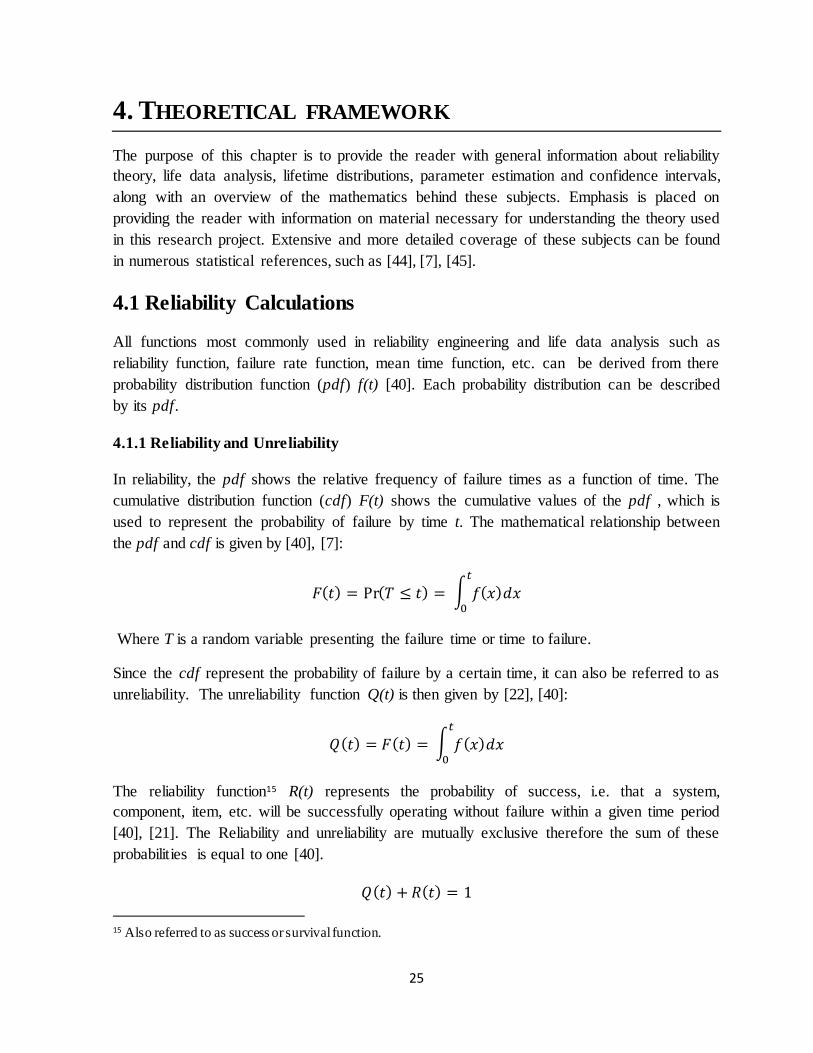
25

4. THEORETICAL FRAMEWORK

The purpose of this chapter is to provide the reader with general information about reliability

theory, life data analysis, lifetime distributions, parameter estimation and confidence intervals,

along with an overview of the mathematics behind these subjects. Emphasis is placed on

providing the reader with information on material necessary for understanding the theory used

in this research project. Extensive and more detailed coverage of these subjects can be found

in numerous statistical references, such as [44], [7], [45].

4.1 Reliability Calculations

All functions most commonly used in reliability engineering and life data analysis such as

reliability function, failure rate function, mean time function, etc. can be derived from there

probability distribution function (pdf) f(t) [40]. Each probability distribution can be described

by its pdf.

4.1.1 Reliability and Unreliability

In reliability, the pdf shows the relative frequency of failure times as a function of time. The

cumulative distribution function (cdf) F(t) shows the cumulative values of the pdf , which is

used to represent the probability of failure by time t. The mathematical relationship between

the pdf and cdf is given by [40], [7]:

𝐹(𝑡) = Pr(𝑇 ≤ 𝑡) = ∫ 𝑓(𝑥)𝑑𝑥𝑡

0

Where T is a random variable presenting the failure time or time to failure.

Since the cdf represent the probability of failure by a certain time, it can also be referred to as

unreliability. The unreliability function Q(t) is then given by [22], [40]:

𝑄(𝑡) = 𝐹(𝑡) = ∫ 𝑓(𝑥)𝑑𝑥𝑡

0

The reliability function15 R(t) represents the probability of success, i.e. that a system,

component, item, etc. will be successfully operating without failure within a given time period

[40], [21]. The Reliability and unreliability are mutually exclusive therefore the sum of these

probabilities is equal to one [40].

𝑄(𝑡) + 𝑅(𝑡) = 1

15 Also referred to as success or survival function.

26

The reliability function is then given by [40], [7], [21]:

𝑅(𝑡) = 1 − 𝑄(𝑡)

𝑅(𝑡) = 1 − ∫ 𝑓(𝑥)𝑑𝑥𝑡

0

𝑅(𝑡) = ∫ 𝑓(𝑥)𝑑𝑥∞

𝑡

𝑅(𝑡) = Pr(𝑇 > 𝑡) 𝑓𝑜𝑟 𝑡 > 0

The three functions, R(t), F(t) and f(t) are closely related to one another. If any of them is

known, all the others can be determined [21] since [7]:

𝑓(𝑡) =𝑑

𝑑𝑡𝐹(𝑡) =

𝑑

𝑑𝑡𝑄(𝑡) =

𝑑

𝑑𝑡(1 − 𝑅(𝑡)) = −𝑅′(𝑡)

In figure 4-1 the relationship between the reliability function and the cumulative distribution

function (unreliability), can be seen. Where the x-axis represents time and y-axis shows how

reliability and unreliability are related and changes in one affect the other.

Figure 4-1: Relationship between reliability and unreliability [43].

4.1.2 Failure rate function

The failure rate function16 𝜆(𝑡) describes the number of failures per time unit, where time can

be any quantifiable measure, such as minutes, hours, cycles, etc. The failure rate is useful in

describing the failure behavior of a components [40], it provides information about the

changing rate in the aging behavior over the life of a population of components [21].

16 Also referred to as the hazard rate and in actuarial statistics referred to as force of mortality [7].

27

The failure rate function is defined as [40], [7], [21]:

𝜆(𝑡) = 𝑓(𝑡)

(1 − 𝐹(𝑡)) =

𝑓(𝑡)

𝑅(𝑡) =

−𝑅′(𝑡)

𝑅(𝑡)= −

𝑑

𝑑𝑡ln 𝑅(𝑡)

Since all parts are assumed to be functional at time t = 0 or R(0) = 1, then by integrating both

sides results in [7]:

∫ 𝜆(𝑢)𝑡

0𝑑𝑢 = − ln 𝑅(𝑡)

𝑅(𝑡) = 𝑒− ∫ λ(u)𝑡

0 𝑑𝑢

The reliability function R(t) and the unreliability function Q(t) = 1 - R(t) are therefore uniquely

determined by the failure rate function 𝜆(𝑡) [7].

4.1.3 The Mean time to failure (MTTF)

The mean time to failure (MTTF) is defined as the expected value of the lifetime before a

failure occurs [21].

MTTF provides a measure of the average time of operation to failure and is given by [21], [7]:

𝑀𝑇𝑇𝐹 = ∫ 𝑡 ∗ 𝑓(𝑡)𝑑𝑡∞

0= ∫ 𝑅(𝑡)𝑑𝑡

∞

0

The MTTF does not give much, if any, information on the failure distribution of the

component. Different distributions can have identical means, so it is unwise to use only the

MTTF when measuring the reliability of the component [40].

MTTF is used for non-repairable systems, for repairable systems the mean time between

failures (MTBF) is used. MTBF is an expected value of the random variable time between

failures. Another important measure that is often used in maintenance studies is the mean time

to repair (MTTR), which is the expected value of the repair time. The mathematical

relationship between these measures is given by [21].

𝑀𝑇𝐵𝐹 = 𝑀𝑇𝑇𝑅 + 𝑀𝑇𝑇𝐹

4.1.4 The Bathtub curve

The failure rate as a function of time can be described graphically, if the time to failure for

enough units from a given population has been observed. The failure rate can be increasing,

28

decreasing or be a combination of those, depending on the component characteristics [40],

[46]. The plot of failure rate versus time typically takes on a characteristic bathtub shape as

shown in figure 4-2. The bathtub curve can be very useful in determining, for example, the

optimum breaking in period, the optimum burn-in time, the optimum preventive replacement

time of components and the optimum warranty period and cost [44].

Figure 3-2: The "Bathtub curve" showing three life stages of failure rate vs. time [45].

The bathtub curve comprises three life stages [47], [23]:

1. The first stage has a decreasing failure rate, known as early failures, infant mortality or

burn-in stage.

2. The second stage has a constant failure rate, known as random failures, useful life or

steady life stage.

3. The third stage has an increasing failure rate, known as wear-out-failures or rapid

breakdown period.

In the initial stages, the failure rate is high but quickly decreases as defective components are

identified. Manufactures often test components before they are distributed to the customers,

that way much of the infant mortality will be removed before the components are delivered to

the costumers [7].

In the middle stage, the failure rate is generally low and constant. Usually considered to be

random failures which are caused by stress exceeding the design strength, for example,

overstress failures due to accidental or transient circuit overload [46]. In this research project

the engines are for example considered to have constant failure rate (see chapter 6.2.1.2)

which is represented by the second stage of the bathtub curve. The main prerequisite for using

a constant failure rate is that engines are being analyzed based on overall behavior of engines,

i.e. behavior on engines on world fleet basis. Essentially it is expected that all engines have the

same fundamental characteristics, especially regarding severe failures which would result in

29

IFSD and therefore making the assumption that the probability of IFSD over the lifetime of

the engines is uniformly distributed.

In the last stage, the failure rate increases as the component begins to wear out, due to fatigue,

depletion of materials, etc.

4.2 Life data analysis

Life data analysis17 refers to the study and modeling of observed item, component, system,

product, etc. lives. By analyzing a sample from a population of a particular component, in

interest, and collecting data on time of success operation or time to failure, predictions can be

made about the population. One of the primary objectives is to obtain a distribution that

describes the time of success operation or time to failure of the component. Once, appropriate

distribution has been found for the data set, it can be used to estimate important life

characteristics of the component, such as the failure rate, reliability or probability of failure at

a specific time and the mean life [40], [22].

Data used in this research project was obtained from Rolls-Royce, Delta Airlines and

Icelandair over the period from 18.01.2010 to 31.03.2016. The collected data gave information

on failures over that period and accumulated fleet hours, whether there was a failure or not.

This information was then used to estimate distributions, which would describe the time to

failure of each component (see chapter 6.2)

4.2.1 Life data classification

In life data analysis, the model is the lifetime distribution and the data are the time to failure of

the component. The lifetime distribution that best fits the data is chosen at each time, if the

supplied data is bad or insufficient it will most likely result in bad prediction. The precision of

any predictions is proportional to the quality, accuracy and completeness of the data [40], [7].

So it is important to consider the type of the supplied data, for example, is all information

included in the data or not. Life data of components can be separated into four types [7];

Complete data

Right censored data (Suspension)

Interval censored data

Left censored data

Each data type requires a modification to the analysis in order to correctly estimate the

underlying lifetime distribution.

17 Also known as Weibull analysis.

30

4.2.1.1 Complete Data

When the supplied data is a complete

data, it means that the value of each unit

in the sample is known, that is the time

to failure of all units in the sample [40].

In figure 4-3, a complete data set of five

sample units is illustrated

4.2.1.2 Right Censored Data

Often some units in the sample have not

failed after a given time (testing time) or

the exact times to failure of all the units

in the sample are not known. This type

of data is called censored data; right

censored data (or suspended data) is

when data sets are composed with units

that did not fail over the test time, and

are therefore still operating [7], [40]. In

figure 4-4, a data set of five sample

units, were two of them contain suspension

is illustrated.

4.2.1.3 Interval Censored Data

When the supplied data is an interval

censored data only the time interval for

when the sample unit failed is known,

not the exact time of failure. In situations

where the components in the sample are

not constantly monitored, however,

inspections are done in a certain time

interval, this type of data is obtained [7],

[40]. In figure 4-5 a data set of five

sample units with interval censoring is

illustrated.

Figure 4-3: Example of complete data sample set [37].

Figure 4-4: Example of data set with suspension [37].

Figure 4-5: Example of Interval censored data [37].

31

4.2.1.4 Left Censored Data

When the supplied data is a left

censoring data, the data sets are

composed with sample units that have

failed but the time of failure is not known

only that the sample unit failed between

time 0 and when it was inspected [7],

[40]. In figure 4-6 a data set of five

samples, were two of them are left

censoring is illustrated.

In this research project the collected data gave information on failure times and accumulated

fleet hours, whether there was a failure or not. This was done to estimate the number of

suspensions for the components i.e. the number of times for when the component did not fail

over the period. So according to life data classification the obtained data is right censored data.

4.2.2 Lifetime distributions

There are many different distributions that can be used to model probability of failure (or the

probability of success). However some distributions tend to better represent life data and are

commonly called lifetime distributions. The most commonly used distributions in the

reliability studies, according to [47] are the Weibull distribution, exponential distribution and

the lognormal distribution [40], [47]. When choosing the appropriate lifetime distribution, the

component s characteristics and failure behavior needs to be considered. Times to failure of

electrical components, for example, are often modeled with the exponential distribution,

because it is often assumed that they do not wear out. On the other hand, the time to failure of

mechanical components are often modeled with the Weibull distribution [48].

In the following sections only the lifetime distributions that the Weibull++ software estimated,

to be best suited, to describe the times to failure for components are presented. These

distributions are the Exponential distribution and the Weibull distribution. In appendix B

information about the Normal distribution and the Lognormal distribution can also be found.

For further information on other distributions, detail coverage can be found in references such

as [7].

4.2.2.1 The Exponential Distribution

The exponential distribution is a very commonly used distribution to model reliability data.

The main reason for this is its mathematical simplicity and that it is often a good

approximation to the actual distribution for certain types of components [49], [7]. An

Figure 4-6: Example data set with left censoring [37]

32

important property of the exponential distribution is that it is memoryless. This means that the

failure rate of an component with exponential distribution is constant i.e. independent of time

and therefore does not have any aging property [7], [21]. Due to its mathematical simplicity

the exponential distribution has been widely used even in cases where it is inappropriate [40].

One of the most typical missteps is the assumption of an exponential distribution and therefor

a constant failure rate behavior for components that do not have a constant failure rate. As a

result, indications of the infant-mortality and wear-out failures are not noticed. This can lead

to inaccurate reliability estimates [50], [51]. However the exponential distribution is a

realistic life distribution for certain types of components, for example electrical components,

where it may be assumed that the component dose not degrades or wear out with time [7],

[52]. The exponential distribution is considered to be a good model for the long flat “intrinsic

failure” portion of the Bathtub Curve (see chapter 4.1.4). Because many components spend the

majority of their lives in this portion of the Bathtub Curve, this often justifies the frequent use

of the exponential distribution [53].

The probability distribution function (pdf) for the exponential distribution is defined as [7],

[49]:

𝑓(𝑡) = { 𝜆𝑒−𝜆𝑡 𝑓𝑜𝑟 𝑡 > 0, 𝜆 > 0 0 𝑜𝑡ℎ𝑒𝑟𝑤𝑖𝑠𝑒

where λ is the failure rate parameter and t is a variable representing the operation time. In

figure 4-7 the pdf for the exponential distribution is illustrated with two different values of the

failure rate, λ equal 0.01 and λ equal 0.005. Changes in pdf are shown on the y-axis while the

x-axis represents time.

Figure 4-7: Exponential pdf with two different values of the failure rate λ [40].

33

The reliability function is [7]:

𝑅(𝑡) = Pr(𝑇 > 𝑡) = ∫ 𝑓(𝑢)𝑑𝑢∞

𝑡= 𝑒−𝜆𝑡 𝑓𝑜𝑟 𝑡 > 0

where T is a random variable presenting the time to failure.

The failure rate function is [7]:

𝜆(𝑡) =𝑓(𝑡)

𝑅(𝑡)=

𝜆𝑒−𝜆𝑡

𝑒−𝜆𝑡 = 𝜆

The mean time to failure is [7]:

𝑀𝑇𝑇𝐹 = ∫ 𝑅(𝑡)𝑑𝑡∞

0= ∫ 𝑒−𝜆𝑡𝑑𝑡

∞

0=

1

𝜆

4.2.2.2 The Weibull Distribution

The Weibull distribution is one of the most commonly used life distribution in reliability and

life data analysis due to its versatility, flexibility and relative simplicity [54], [55]. Depending

on the values of the parameters, the Weibull distribution can take on the characteristics of

other types of distributions and be used to model many types of failure rate behaviors [7].

Analysis of the Weibull distribution can also be useful in providing information needed for

troubleshooting, scheduling preventive maintenance, scheduling inspections and classifying

failure types [54]. The pdf for the 2-parameter Weibull distribution is given by [40], [56]:

𝑓(𝑡) = {𝛽

𝜂(

𝑡

𝜂)

𝛽−1

𝑒−(𝑡

𝜂)

𝛽

𝑡 ≥ 0

0 𝑜𝑡ℎ𝑒𝑟𝑤𝑖𝑠𝑒

where β is the shape parameter18, η is the scale parameter19 and t is a variable presenting time.

The shape parameter β determines the basic shape of the function, the impact of the parameter

is reflected in the shapes of the pdf, the failure rate function and the reliability function [40].

18 Also known as the Weibull slope, because β is equal to the slope of the regressed line in a probability plot [40]. 19 Known as scale parameter or characteristic life.

34

Figure 4-8: Weibull pdf with three different values of the shape parameter β [40].

In figure 4-8 the pdf for the Weibull distribution is illustrated with three different values of the

shape parameter, β equal to 0.5, β equal to 1 and β equal to 3.The scale parameter η is fixed.

Changes in pdf are shown on the y-axis while the x-axis represents time. In the above figure it

can be seen how different values of β affect the shape of the pdf. Varying the values of β can

also have huge impact on the failure rate of the Weibull distribution and important

assumptions can be made about the components failure characteristics by considering the

value of β.

Figure 4-9: Weibull failure rate with three different values of the shape parameter β [40].

In figure 4-9 the failure rate function of the Weibull distribution is illustrated with three

different values of β and fixed η. Changes in the failure rate function are shown on the y-axis

while the x-axis represents time. From the figure it can be seen that the Weibull distribution

can be used to model life distributions where the failure rate is decreasing, constant or

35

increasing and is therefore capable to model all three life stages of the bathtub curve (see

chapter 4.1.4) [7]. Because of this flexibility the Weibull distribution is considered to be a

realistic distribution for many types of components [40].

The scale parameter η indicates where the bulk of the distribution lies, or how stretched out it

is. The larger the η, the more spread out. The smaller it is, the more squeezed [40].

Figure 4-10: Weibull pdf with three different values of η [40].

In figure 4-10 it can be seen how changing the value of η, with fixed β, can impact the Weibull

pdf.

The reliability function for the 2-parameter Weibull distribution is [40]:

𝑅(𝑡) = Pr(𝑇 > 𝑡) = 𝑒−(𝑡

𝜂)

𝛽

𝑓𝑜𝑟 𝑡 > 0

where T is a random variable presenting the time to failure.

The failure rate function is [40]:

𝜆(𝑡) =𝑓(𝑡)

𝑅(𝑡)=

𝛽

𝜂(

𝑡

𝜂)

𝛽−1


The mean time to failure is [40], [7]:

𝑀𝑇𝑇𝐹 = ∫ 𝑅(𝑡)𝑑𝑡∞

0= ∫ 𝑒

−(𝑡𝜂

)𝛽

𝑑𝑡 ∞

0= 𝜂 ∗ Γ (

1

𝛽+ 1)

36

where Γ (1

𝛽+ 1) is the gamma function, calculated with the value given by (

1

𝛽+ 1).

The gamma function is defined as [40]:

Γ(𝑡) = ∫ 𝑒−𝑥 𝑥𝑡−1𝑑𝑥∞

0

Further information on gamma function can be found in references such as [7] and [40].

4.2.3 Parameter Estimation

In parameter estimation, sample data (times to failure or success data) is used to estimate the

parameters of the distribution that was selected. There are several methods to estimate the

parameters to fit a lifetime distribution to a particular data set, and different methods produce

different estimates. Typical parameter estimation methods are [40], [57];

Least Squares (Linear Regression)

Maximum Likelihood Estimation

Bayesian Methods

In the least squares parameter estimation method the values of the unknown parameters are

estimated by finding numerical values for the parameters that minimize the sum of squared

discrepancies between observed data, on the one hand, and their expected values on the other.

A line is fitted to the data points, so that the sum of the squares of the distance from the points

to the line is minimized. This can be done in either vertical or horizontal direction. The

method is considered quite good for functions that can be linearized [40], [58].

The maximum likelihood estimation (MLE) involves finding the most likely values of the

unknown parameters that will best describe the data, for a given distribution, that is, the

parameter that maximizes the likelihood of the observed data. The MLE is considered to be a

powerful method for large sample sizes, but with small sample sizes the method can be very

biased [40], [57].

In both least squares parameter estimation and MLE classical statistics are used. In Bayesian

analysis methods, Bayesian statistics are used. The main difference is that in classical

statistics, parameters are fixed numerical values, but in Bayesian statistics the true numerical

value of the parameters can be treated as a random variable to which the analysist assigns a

probability distribution, known as prior information [59]. So in Bayesian statistics prior

knowledge is taken into account, along with a given set of current observations. This prior

knowledge could, for example, come from operational or observational data, from engineering

37

knowledge or previous comparable experiments [40], [7]. When there is a lack of data, when

analyzing reliability and risk, this prior knowledge can be very useful.

4.2.3.1 Confidence bounds

When performing life data analysis the results are an estimate based on the observed lifetimes

of the sample components, due to limited sample size there is always an uncertainty involved

in the results. Confidence bounds are used to quantify this uncertainty due to this sampling

error. By employing confidence bounds a range of plausible values for the estimated

parameter is obtained. Confidence bounds can be expressed as one-sided or two-sided. Using

two-sided confidence bounds means that there is a closed interval and the true value lies

within this interval with a specific certainty. One-sided confidence bounds are either upper

bounds or lower bounds. With a upper bound, the true value is with a certain present below a

specific point and the opposite for the lower bound. As an example when using 90% two-sided

confidence bounds in parameter estimation, it can be estimated with 90% certainty that the

true value of the parameter lies within the interval, in 5% of the time it is below the lower

bound and in 5% of the time it is above the upper bound [40].

39

5. METHODOLOGY

The reliability of the system will be analyzed using the Reliability Block Diagram (RBD)

approach. A RBD model of the system will be built using the commercial BlockSim 10

software. The reliability model will be analyzed by simulating the model in the software.

BlockSim will also undertake all computations that the RBD approach is based on. The model

will also be analyzed with analytical calculations, however when analyzing the model over

different phases of a flight (i.e. take off, climb, cruise, descent and landing) analytical

calculations can get extremely difficult. In such cases simulation is more suitable.

The main purpose of this chapter is to provide an overview of the RBD approach along with

the associated mathematical formulation needed in this research project. Similarly this chapter

also gives an overview of Reliability Phase Diagram (RPD) method and other features used in

BlockSim to model the system.

5.1 Reliability Block Diagrams (RBD)

A RBD model provides a success-oriented view of the system, showing all essential functions

required for system operation. It is a graphical representation of how the components of a

system are connected from a reliability point of view. RBD also provides a good framework

for understanding the redundancy of the system. RBD blocks are used to represent

components of the overall system and to define success paths, for the system to be

functioning i.e. successfully operational, a functioning path must exist between the start point

and the end point of the diagram [7], [32], [33]. An example of a RBD can be seen in figure

5-1. In this system there are ten components, components one, two and tree are connected

reliability-wise in series, which means that all three of them have to be functioning for the

overall system to be functioning. Components nine and ten are connected reliability-wise in

parallel, which means that either one of them has to be functioning, not both, for the overall

system to be functioning, i.e. there is a redundancy. Components four to eight are combined in

a series and parallel configuration. In this diagram there are six potential flow paths through

the system, but only one of them has to be functioning for the overall system to be

functioning.

40

Figure 5-1: Example of Reliability Block Diagram [55].

When modeling a RBD a detailed understanding of the overall system is necessary, a

commonly used approach is to break the system into subsystems or components from a top-

down point of view. The level of detail in segmenting the system should be based on both the

availability of data and the lowest level of actionable component [22], [34]. When the system

has been segmented to a desired level of accuracy, blocks in the diagram and their connections

can be defined. Once necessary data has been obtained, lifetime distributions can be defined

for each component, along with reliability and other characteristics of the component. When

these reliability characteristics of all components that make up the system are known, the RBD

can be used to calculate the overall system reliability [22], [35].

In the following subsections an overview of different RBD configurations will be presented.

5.1.1 RBD configuration

A RBD shows in a graphical way the reliability wise connection between components in a

system. Each block in the diagram represents a component of the overall system. Blocks can

be connected in different ways depending on the system being analyzed. The structure of the

components in a system can be in, for example, series structure, parallel structure, k-out-of-n

structure, load sharing structure, complex structure, standby structure or some combination of

these structures. The main structures that can be used in the BlockSim software and those that

are used in this research project are described in the following subsections.

5.1.1.1 Series Structure

When a system has a series structure, all blocks are connected reliability-wise in series. The

system is functioning only if all of its components are functioning, so if one component fails it

results in a failure of the entire system. In other words, all of the components in a series

system must succeed for the system to succeed. The reliability of such system is always less

41

than the reliability of the least reliable component and the system reliability decreases as more

components are added [7], [22],[47]. An example of a series structured system with three

components can be seen in figure 5-2.

Figure 5-2: Example of a series structured system [14].

The system reliability (𝑅𝑠) of a system with n components in series structure is given by

[7],[22]:

𝑅𝑠 = 𝑅1 ∗ 𝑅2 … 𝑅𝑛 = ∏ 𝑅𝑖

𝑛

𝑖=1

5.1.1.2 Parallel Structure (Redundancy)

When a system has a parallel structure, all blocks are arranged reliability-wise in parallel. The

system is functioning if at least one of the components is functioning, so all components must

fail in order for the system to fail. In other words, success of any component in the system

results in a system success [7], [22]. A system with components connected in parallel is said to

be a redundant system [47]. Redundancy is a very important aspect of system design and

reliability, because by adding redundancy, that is, having several identical or similar

components to perform the same function within the system, the reliability of the system can

be improved [57]. Redundancy is widely used in the aerospace industry and with electronic

products and safety systems to achieve higher reliability [22], [57]. For systems with parallel

structure, the component with the highest reliability has the biggest effect on the systems total

reliability. Opposite to the series structure system, by increasing the number of components in

a parallel system, the system s reliability increases [22]. An example of parallel structured

system with n components can be seen in figure 5-3.

42

Figure 5-3: Example of a parallel structured system [14].

The system reliability (𝑅𝑠) of a system with n components in a parallel structure is given by

[7], [22]:

𝑅𝑠 = 1 − (1 − 𝑅1)(1 − 𝑅2) … (1 − 𝑅𝑛) = 1 − ∏(1 − 𝑅𝑖)

𝑛

𝑖=1

5.1.1.3 k-out-of-n Structure

When a system has a k-out-of-n structure, the system is considered to be functioning if at least

k out of a total of n components is functioning. This is a special case of the parallel

redundancy, where at least k components have to succeed for the system to succeed. As the k

number of component needed increases compared to the total of n components, the system

structure moves closer to being a series structure. Thus, with increasing k compared with n, the

reliability decreases. A series structure is therefore an n-out-of-n structure and parallel

structure is a 1-out-of-n structure [7], [22]. A note block is used to specify the k number of

component required for the entire system to be functional [21]. An example of k-out-of-n

structured system can be seen in figure 5-4. This is a system with two out of three structure,

the node specifies that two components out of three must be functional for the system to be

functional.

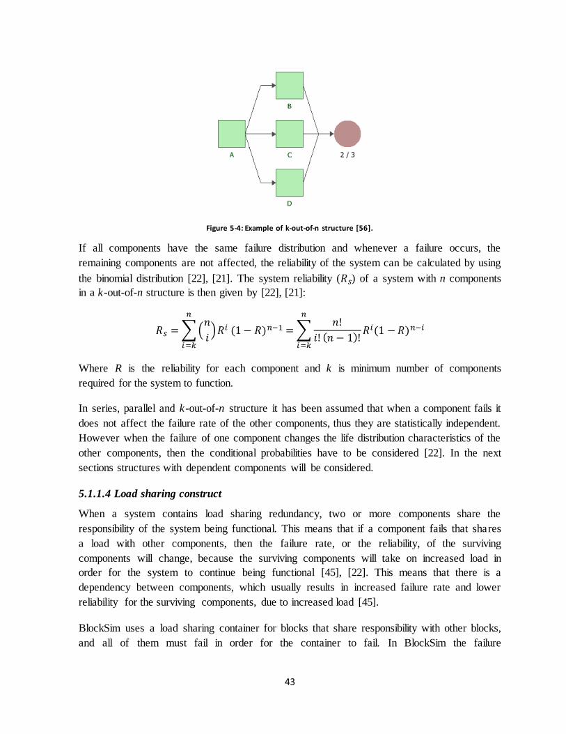
43

Figure 5-4: Example of k-out-of-n structure [56].

If all components have the same failure distribution and whenever a failure occurs, the

remaining components are not affected, the reliability of the system can be calculated by using

the binomial distribution [22], [21]. The system reliability (𝑅𝑠) of a system with n components

in a k-out-of-n structure is then given by [22], [21]:

𝑅𝑠 = ∑ (𝑛

𝑖)𝑅𝑖

𝑛

𝑖=𝑘

(1 − 𝑅)𝑛−1 = ∑𝑛!

𝑖! (𝑛 − 1)!

𝑛

𝑖=𝑘

𝑅𝑖(1 − 𝑅)𝑛−𝑖

Where R is the reliability for each component and k is minimum number of components

required for the system to function.

In series, parallel and k-out-of-n structure it has been assumed that when a component fails it

does not affect the failure rate of the other components, thus they are statistically independent.

However when the failure of one component changes the life distribution characteristics of the

other components, then the conditional probabilities have to be considered [22]. In the next

sections structures with dependent components will be considered.

5.1.1.4 Load sharing construct

When a system contains load sharing redundancy, two or more components share the

responsibility of the system being functional. This means that if a component fails that shares

a load with other components, then the failure rate, or the reliability, of the surviving

components will change, because the surviving components will take on increased load in

order for the system to continue being functional [45], [22]. This means that there is a

dependency between components, which usually results in increased failure rate and lower

reliability for the surviving components, due to increased load [45].

BlockSim uses a load sharing container for blocks that share responsibility with other blocks,

and all of them must fail in order for the container to fail. In BlockSim the failure

44

characteristics of each block is defined using both a lifetime distribution and a life-stress

relationship that describes how the lifetime distribution changes as the load changes. In figure

5-5 an example of a system with load sharing container can be seen.

Figure 5-5: Example of blocks in a load sharing container [14].

When dealing with a load sharing redundancy and therefore a component dependence, the

system becomes much more complex. Hence, calculating the system reliability can be very

complex as well. For that reason only the formulation of the reliability function for a load

sharing container with two components will be shown.

The reliability at some time t of a load sharing container with two components can be

calculated with the following equation [60]:

𝑅(𝑡) = 𝑅1(𝑡, 𝑆1) ∗ 𝑅2(𝑡, 𝑆2)

+ ∫ 𝑓1(𝑥, 𝑆1) ∗ 𝑅2(𝑥, 𝑆2) ∗ (𝑅2(𝑡1𝑒 + (𝑡 − 𝑥), 𝑆)

𝑅2(𝑡1𝑒 , 𝑆))

𝑡

0𝑑𝑥

+ ∫ 𝑓2(𝑥, 𝑆2) ∗ 𝑅1(𝑥, 𝑆1) ∗ (𝑅1(𝑡2𝑒 + (𝑡 − 𝑥), 𝑆)

𝑅1(𝑡2𝑒 , 𝑆)) 𝑑𝑥

𝑡

0

Where 𝑓1is the pdf for component one and 𝑓2 is the pdf for component two. 𝑅1 is the reliability

for component one and 𝑅2 the reliability for component two. 𝑆1 and 𝑆2 represent the load

share that component one and two must support when both components are functioning and 𝑆

is the total load. 𝑆1 = 𝑃1𝑆 and 𝑆2 = 𝑃2𝑆, where 𝑃1and 𝑃2 represent the portion of the total load

that each component is supposed to supply when both components are functioning. 𝑡1𝑒 is the

equivalent operating time for component one if it had been operating at 𝑆 instead of 𝑆1and 𝑡2𝑒

is the equivalent operating time for component two if it had been operating at 𝑆 instead of 𝑆2.

45

5.1.1.5 Stand-by Construct

When a system contains standby redundancy, some components are available in standby state.

Standby components are inactive until they are needed, that is they are activated or switched

on when a component in the primary system fails [47]. So, a standby construct is a k-out-of-n

structure, where k out of n components are required to be in an active state while the

remaining components are in a standby state. The system reliability improves when it has a

standby redundancy [22].

BlockSim uses a container with other blocks inside it to represent the components that are in

an active and standby state. The purpose of the container is to define the standby relationship

between an active component and standby components, and also to control the switching

process. Failure distributions for each state have to be defined in BlockSim and it is also a

possibility to define the probability that a switch will successfully activate a standby

component when needed [22], [32]. An example of a system that contains a standby

redundancy can be seen in figure 5-6. The container in the figure contains three components,

one component that is in an active state and two components that are in a standby state.

Figure 5-6: Example of blocks in a standby container [15].

As with load sharing redundancy, the complexity of the system increases rapidly when it

includes standby container. Hence, calculating the system reliability can be very complex as

well. For simplification only the formulation of the reliability function for a standby container

with two components will be shown.

Before formulating the following two assumptions had to be made [47]:

1. The switching system does not fail and there are no delays, so the standby component

is activated instantaneously when primary component fails.

2. The standby component does not fail while it is in a standby state.

46

The reliability at some time t of standby container with two components can be calculated

with the following equation [61]:

𝑅(𝑡) = 𝑅1(𝑡) + ∫ 𝑓1(𝑥)𝑡

0∗ 𝑅2,𝑠𝑏(𝑥) ∗

𝑅2,𝐴(𝑡𝑒 + 𝑡 − 𝑥)

𝑅2,𝐴(𝑡𝑒)𝑑𝑥

Where f1is the pdf for the active component and R1 is the reliability for the active component.

R2,sb is the reliability for the standby component when it is in an standby state. R2,A is the

reliability of the standby component when it is in an active state. t1e is the equivalent

operating time for component one if it had been operating at S instead of S1 and t2e is the

equivalent operating time for the standby component if it had been operating at an active state

[61].

5.2 Analyzing the RBD Model

When the lifetime distributions for each component (block) in the system have been defined,

the components can be connected in a way that represents the reliability-wise configuration of

the system. Once the RBD model for the system has been constructed, an overall system

reliability calculation can be made. The analysis method used for computing the reliability of

the system can be made either by an analytical approach or a simulation [22],[62]. Using

analytical approach to analyze the RBD involves determining exact mathematical expression

that describes the reliability of the system [36]. When modeling complex system it gets harder

and often quite time consuming to obtain analytical solution. If the system is repairable and

maintenance actions have to be included, solving them analytically becomes extremely

difficult or even impossible. In those cases, when the system is repairable or very complex,

analysis through simulation becomes necessary to obtain information on the systems reliability

and/or availability [22].

In BlockSim both Analytical calculation and simulation can be performed. The analytical

approach should be used when considering only the failure characteristics of the components.

When the system is repairable and both failure and maintenance characteristics are considered,

then it’s necessary to use simulation, where it might be impossible to compute an analytical

solution. By using the simulation methods additional events like repair, maintenance and

restoration action can be included in the model [22], [62], [36].

5.2.1 Analytical analysis

Using analytical approach to analyze the RBD involves determining exact mathematical

expression that describes the reliability of the system, after the reliability-wise configuration

for components (blocks) has been defined along with lifetime distributions for each

component the reliability function (mathematical expression) can be obtained.

47

The reliability function describes the reliability of the system as a function of time based on

the lifetime distributions of its components, i.e. from the probability distribution (pdf) for each

component [22].

After the systems reliability function has been obtained, the reliability and other metrics in

interest can be calculated. Such calculations include for example [36]:

1. Calculating the pdf for the system

2. Calculating the failure rate for the system

3. Calculating the MTTF for the system

4. Calculating the exact values of the reliability at specific points in time

5. Calculating reliability importance measures for the components of the system

Two types of analytical calculations can be performed using RBD, static and time-dependent

calculations. Systems can contain either one or a mixture of static and time-dependent blocks,

i.e. components in the system can have a fixed probability of success/failure independent of

time and components wherein a lifetime distribution is assigned to the component and

success/failure is time-dependent (reliability will be a function of time) [22].

5.2.2 Monte Carlo (MC) Simulation

When performing a reliability analysis, there are many techniques that can be used. The most

commonly used techniques are RBD, network diagrams, fault tree analysis and MC

simulation[21]. Computer simulation has served as an important tool in many fields, such as

engineering, economics, biology, medicine, chemistry and many others fields. Through

computer simulation, the behavior of real-life systems are studied [63].

MC simulation is used to imitate the behavior of real-life systems. After the model has been

built and all failure distributions (lifetime distributions) estimated, along with all additional

events such as maintenance actions, the model representing the system can be simulated. MC

simulation generates a random failure times from each components failure distribution in the

system. These randomly generated failure times are then combined in accordance with the way

the components are reliability–wise connected in the system [22], [24]. In general models have

to be simulated multiple times, i.e. MC simulation can consist of multiple iterations, to obtain

an estimate of the real-life system. After results from the simulation have been obtained the

reliability and other matrices in interest, both for the entire system and its components, can be

calculated [24].

48

5.3 Reliability Phase Diagrams (RPD)

RPDs are used as an extension of the RBD approach. When only RBD are used to analyze the

reliability of a system, the system cannot undergo any changes over the operating time, i.e. the

system has a fixed configuration. On the other hand if RPD are used with RBD, it becomes

possible to analyze system that might undergo changes in its reliability configuration and/or

changes in other properties of the system or components over the operating time [22],[32].

The BlockSim software uses RPDs to analyze systems, through simulation, that undergo such

changes over the operating time.

5.3.1 Phase blocks

In the BlockSim software, phase blocks are used to build a RPD and each phase block

represents a certain stage in the operation of the system. Each phase is linked to a relevant

RBD that describes the reliability-wise configuration of the system (and other properties)

during that stage of the operation time. Phase blocks in the RPD are arranged in chronological

order to describe each sequential stage in the operation of the system [22], [32].

In the BlockSim software, there are two kinds of phase blocks that can be used in RPD,

operational phase and maintenance phase.

5.3.1.1 Operational Phases

An operational phase is used to describe any stage in the operation of the system, except for

the maintenance actions that are executed in the maintenance phase. Operational phases are

always linked to a RBD, which describes the reliability-wise configuration of the system at

that stage. For each operational phase in the RBD the duration needs to be specified and it is

also a possibility to specify different stress loads (phase duty cycle) between operational

phases [22].

5.3.1.2 Maintenance phases

A maintenance phase is used to describe the portion of the systems operation time where the

system is down and maintenance actions are executed whether they are scheduled or

unscheduled actions. Wherein no maintenance actions are included in this research project the

maintenance phase will not be discussed in more detail, for further information see references

such as [22], [32].

5.3.2 Simulation of RPDs

In BlockSim RPDs are analyzed though simulation, before simulation can begin, success and

failure paths need to be defined. When the RPD is simulated the movement from the first

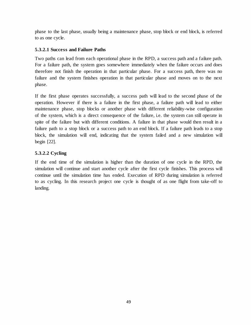
49

phase to the last phase, usually being a maintenance phase, stop block or end block, is referred

to as one cycle.

5.3.2.1 Success and Failure Paths

Two paths can lead from each operational phase in the RPD, a success path and a failure path.

For a failure path, the system goes somewhere immediately when the failure occurs and does

therefore not finish the operation in that particular phase. For a success path, there was no

failure and the system finishes operation in that particular phase and moves on to the next

phase.

If the first phase operates successfully, a success path will lead to the second phase of the

operation. However if there is a failure in the first phase, a failure path will lead to either

maintenance phase, stop blocks or another phase with different reliability-wise configuration

of the system, which is a direct consequence of the failure, i.e. the system can still operate in

spite of the failure but with different conditions. A failure in that phase would then result in a

failure path to a stop block or a success path to an end block. If a failure path leads to a stop

block, the simulation will end, indicating that the system failed and a new simulation will

begin [22].

5.3.2.2 Cycling

If the end time of the simulation is higher than the duration of one cycle in the RPD, the

simulation will continue and start another cycle after the first cycle finishes. This process will

continue until the simulation time has ended. Execution of RPD during simulation is referred

to as cycling. In this research project one cycle is thought of as one flight from take-off to

landing.

51

6. RELIABILITY OF THE ELECTRICAL SYSTEM IN

BOEING 757-200 AIRCRAFT

In this chapter an overview of the electrical system in Boeing 757-200 aircrafts is provided

along with an explanation on of how the engines and APU are configured in the electrical

system. Moreover the difference in the electrical system between Boeing 757-200 aircraft with

three generators and aircraft with four generators (HMG as the fourth) is illustrated and

explained in more detail. Information on data collection and how data was processed is also

covered. Then finally a description of how the RBD, which is covered in chapter 5, is used to

build a reliability model of the systems.

6.1 Overview20 of the electrical system in Boeing 757-200 aircraft

The Boeing 757-200 has three non-time limited independent power sources. Primary power is

supplied by two engine-driven integrated drive generators (IDG). The third power source is an

Auxiliary power unit (APU)-driven generator, which provides an in-flight back-up for the two

main engine-driven IDG. The primary alternating current (AC) system is divided into left and

right main AC buses as can be seen in figure 6-1. Each channel consists of a main AC bus

supplied by an associated IDG. Both the IDG s provide separately 90 KVA power to the

aircraft systems. The APU generator also provides 90 KVA power to the aircraft systems. The

power provided from each one of these generators is sufficient to power all of the aircraft

critical systems. In figure 6-1, it can be seen how the left IDG, right IDG and APU generator

are connected to the main AC buses. If an in-flight generator shutdown or a power source

overload occurs during flight then all non-essential loads on both main AC buses are de-

energized, which is called load shedding. The entertainment system (TV screens) is an

example of non-essential load that would be turned off if needed. During two generator

operation, the 757 electrical power system can supply all required electrical power, without

de-energizing any loads. However during single generator operation, the total aircraft load

demands can exceed the capacity of one generator. Automatic load shedding will then de-

energize non-essential loads to prevent generator overload.

20 All Information’s about the electrical system were obtained from Boeing 757 training manuals, General Familiarization Manuals such as [64] and Electrical load analysis obtained from Icelandair Technical Services.

52

Figure 6-1: Electrical System Overview [64].

External Power Source can be connected to the AC tie bus through the external power

contactor (EPC), which can be seen in the figure as well, this however can only be done when

the aircraft is on ground. External power will not be considered in this research project since

the system is being analyzed when in flight. The generator control units (GCU), which are also

shown in the figure, provide automatic control and protection functions for each channel by

monitoring IDG output. The GCU provides protective trip commands to the generator circuit

Breaker (GCB) and/or bus tie breaker (BTB) to prevent load and source equipment damage if

faults or failures occur in the system.

In this research project only the RB211-535E4-B engines (which Icelandair operates), IDGs,

APU generator, in-flight start on APU and HMG are considered. These are the critical

components in the system and each of them will be presented with a single block in the model.

The reason for not breaking those components further down is because only severe failures

that cause complete loss are being considered. Furthermore data on subcomponent level would

be difficult, where such detailed data is often not available.

GCU, GCB, BTB, and main AC buses are not included in the model (see figure 6-1), however

these components need to be functioning correctly to supply electrical power the aircrafts

systems. In this research project the main focus is on showing that the reliability of the

generators are sufficient and that they are capable of feeding the AC buses. If failure occurs in

BTB, GCB, and GCU or if the AC bus itself fails, it is irrelevant to the generators, they could

still be in a good condition. Furthermore the structure of the system, concerning the BTB,

GCB, GCU and AC buses is the same whether the aircraft has ETOPS approval or not so the

reliability for those components should be the same whether the aircraft is ETOPS or non-

53

ETOPS. Also, according to Icelandair Technical Service (ITS) expert’s21 failures in BTB,

GCU, GCB and the AC buses are very rare, at least failures that would result in loss of AC

buses so that aircraft system could not be powered. Failures in the generators themselves are

more likely to be the cause of power loss. If these components would however be included in

the model, their effect would be expected to be negligible on the system reliability results,

wherein failures occur on a much larger time interval than a failure of generators.

6.1.1 Difference between electrical systems with and without HMG

The HMG which is today installed in all Boeing 757-200 aircrafts with ETOPS approval

provides additional electrical power. A HMG, capable of providing additional 5 KVA

electrical power is installed for 120 minute ETOPS and a 10 KVA for 180 minute ETOPS

approval. When a total loss of main power is sensed (i.e. both IDGs and APU generator are

out) then the HMG automatically activates and provides power to critical flight loads.

In appendixes C and D electrical power block diagrams, obtained from Icelandair Technical

Services, can be seen, one without an HMG and the other with an HMG. A red line has been

drawn to highlight which systems the standby system supplies power to upon loss of main

power. In electrical system without HMG, the main battery will supply back-up power to

flight critical loads upon loss of all main power, however it is only capable of supplying

power for a certain amount of time depending on the battery capacity e.g. 30 or 60 minutes.

When a HMG is installed a hydraulic power is supplied to the HMG from the left hydraulic

system when a total loss of AC power (main power) is sensed. The HMG provides power to

all flight critical loads and is non-time limited. However the left hydraulic system is driven by

the left engine; if the left engine fails and the left hydraulic system loses pressure, then a

power transfer unit (PTU) is activated. The PTU will supply the left hydraulic distribution

system with pressure from the right hydraulic pump system and thus provide power to the

HMG.

The main difference is that an electrical system without HMG is not capable of supplying

power to the flight instrument bus22 upon loss of all main power (see appendixes C and D),

whereas a system with HMG can. Furthermore the HMG is non-time limited, but the battery is

time limited.

6.2 Failure data and estimation of lifetime distributions

Data used in this research project was obtained from Rolls-Royce, Delta Airlines and

Icelandair over the period from 18.01.2010 to 31.03.2016. The collected data gave information

21 Heimir Ö. Hólmarsson and Geirfinnur S. Sigurðsson 22 Fl ight instrument bus provides power to selected flight instrument´s, such as speed indicator and altimeter.

54

on failures over that period, which resulted in complete loss of engine (i.e. engine shut-down),

and IDG and APU generator failures and the number of times that the APU could not be

started. Data on accumulated fleet hours, whether there was a failure or not, were also

provided to estimate the number of suspensions23. The Weibull++ software, developed by

Reliasoft Inc., was used to fit a failure distribution (or lifetime distribution24) to the data and

obtain relevant model parameters for each type of component. Thus it is assumed that all IDG

generators are identical in terms of reliability performance. When the failure distribution for

each component type has been estimated, the reliability of the system and other reliability

metrics of interest can be calculated. The Weibull++ software uses Maximum likelihood

estimation25 (MLE) to estimate the parameter values, where all data used contained

suspensions and also because of the large size of the data sets.

Data on engines was collected on a world fleet basis, as regulations require. Data concerning

IDGs was collected from Icelandair Technical Service (ITS). There are no requirements that

the data on generators should be on a world fleet basis. Data concerning APU generator and

APU start in-flight was obtained from both ITS and Delta Airlines, ITS database was not

considered large enough so Delta Airlines provided data as well to support the making of this

research project.

For reasons of confidentiality, the data itself cannot be displayed in this thesis.

6.2.1 Failure models for RB211-535 Engines

In this section only the engines and data concerning them are considered. Data to estimate the

failure distribution for engines (based on IFSD events) was obtained from Rolls-Royce, the

producer of the engine. The family of the RB211 engines can be divided into three distinct

series; RB211-535, -22 and -524. There are three types of the RB211-535 engines; the RB211-

535E4, -535E4B and-535C. Icelandair operates the RB211-535E4 and -535E4B, so only those

engine types are being considered in this research project.

6.2.1.1 Data on number of IFSD on a world fleet basis

Data on engines was obtained on a world fleet basis from Rolls-Royce over the period from

18.01.2010 to 31.03.2016. The data provides information on the number of IFSD events over

that period, the accumulated flight hours of each engine when an IFSD occurred and the total

number of engine hours on a world fleet basis over that same period.

23 See chapter 4.2.1 for further information. 24 See chapter 4.2.2 for further information. 25 See chapter 4.2.3 for further information

55

According to Icelandair s power plant engineers the average engine time before overhaul is

21.450 flight hours. After overhaul the engine is considered to be in “as good as new”

condition. The average operating time before overhaul was therefore considered a valid

estimate of the time at which suspension26 occurred. The flight hours for engines that did not

fail over that same period is therefore estimated to be 21.450 hours.

According to the data total engine hours for RB211-535E4/535E4B over the period were

14.416.475 hours and a total of 91 IFSD occurred. Using the average time before overhaul as

the maximum usage for engines that did not fail, then the number of suspensions could be

estimated, as shown in table 6-1;

Table 6-1: Engine data and estimation of number of engines that did not fail

Engine Data

Total Flight hours on a world fleet basis 14.416.475 hrs.

Sum of accumulated flight hours for all events when IFSD occurred 1.004.137 hrs.

Total success time (accumulated) for engines that did not fail 13.412.338 hrs.

Average time between overhaul 21.450 hrs. Estimated number of engines that did

not fail (number of suspensions) 625 engines

6.2.1.2 Lifetime distribution and parameters for engines

From the data obtained from Rolls-Royce and estimation on suspension times, the failure

distribution that best describes the failure behavior of engines, with respect to IFSD, could be

generated.

Table 6-2: Distribution of RB211-535 failures generated from Rolls-Royce data

Failure distribution for engine

Distribution Parameter

Exponential λ=0,0000062455

As can be seen in table 6-2, results from using the Weibull++ software implied that the

exponential distribution27 with a constant failure rate of λ = 0,625 ∗ 10−5 failures/hour and

26 See chapter 4.2.1.2 for further information. 27 See chapter 4.2.2.1 for further information.

56

therefore an MTTF of 160.115 engine hours (i.e. between IFSDs) on a world fleet basis would

be best suited to describe the data.

Using an exponential distribution with a constant failure rate can be justified. Due to

preventive maintenance actions, servicing actions and corrective line maintenance, the failure

rate for IFSD can be considered as being constant. Moreover when analyzing the probability

of failure on a mission that consists of only a few hours flying time with stress loads that are

the same whether it is an ETOPS or non-ETOPS flight it was considered realistic to conclude

that a constant failure rate of IFSD over the flight can be assumed.

6.2.2 Failure models for IDGs

In this section only the IDGs and failure data concerning them are considered. Data to estimate

the failure distribution for IDGs was obtained from ITS over the period from 18.01.2010 to

31.03.2016. The data provided information on accumulated flight hours for the IDGs when

failure occurred as well as accumulated flight hours for the Boeing 757-200 fleet operated by

Icelandair.

According to the data, total flight hours for the fleet over this period were 433.832 hrs. In each

Boeing 757-200 aircraft there are two IDGs, one is driven by the left engine and the other is

driven by the right engine, hence this results in a total of 867.664 flight hours for IDGs over

this period.

To estimate the number of IDG that did not fail and the times at which suspensions occurred,

the mean time between failures (MTBF) was used as a maximum usage for the IDGs. Data on

MTBF were obtained from the manufacturer of the IDG, Hamilton Sundstrand and was

calculated as an average of a 12 month rolling average from November 2014 to October 2015,

which results in a MTBF of 22.268 flight hours. Using the MTBF as a maximum usage for

IDGs that did not fail, then the number of suspensions could be estimated, as shown in

following table 6-3;

Table 6-3: IDG data and estimation of number of IDGs that did not fail

IDG Data

Total Flight hours

867.664 hrs.

Sum of accumulated fl ight hours for all events when failure occurred

341.314 hrs.

Total success time (accumulated) for IDGs that did not fail

526.350 hrs.

Average time between failure on world fleet basis

22.268 hrs.

Estimated number of IDGs that did not fail (number of suspensions)

24 IDGs

57

6.2.2.1 Lifetime distribution and parameters for IDGs

From the data obtained from Icelandair and estimation on suspension times, the failure

distribution that best describes the failure behavior of IDGs could be generated.

Table 6-4: Failure distribution for IDGs

Failure distribution for IDG

Rank Distribution Parameter

1 Weibull β=0,73454, η=15.995

2 Exponential λ = 0,639468 ∗ 10−4

As can be seen in table 6-4, results from using the Weibull++ software implied that the

Weibull distribution28 with parameters β = 0,73454 and η = 15.994 hrs. could be used to

describe the data. Results also implied that the exponential distribution with MTTF = 15.638

hrs. and a constant failure rate of λ = 0,639468 ∗ 10−4 failures/hour could be used.

6.2.3 Failure models for APU generator

Data to estimate the failure distribution for the APU Generator was obtained from both ITS

and Delta Airlines over the period from 18.01.2010 to 31.03.2016. All data gathered on the

failures of APU generators contained both failure times and suspension times and therefore

there was no need to perform estimation on the number of suspensions and the times at which

suspensions occurred.

6.2.3.1 Lifetime distribution and parameters for APU generator

The APU generator is usually not running unless a failure, causing one of the main generators

to fail, has occurred. Due to the fact that the APU generator is a backup generator and not

always in use, keeping track of actual use of the generator is more complex. Most airlines

record failure times for the APU generator in terms of aircraft hours, i.e. for how long has the

APU generator been installed on the aircraft before a failure occurred. This however does not

describe the actual usage of the generator. Therefore, most airlines make the assumption that

the APU generator is on average in use for one hour per each cycle that the aircraft flew after

the generator was installed and until a failure occurred. From the data obtained from Delta and

the above estimate of APU hours per cycle, the failure distribution that best describes the

failure behavior of APU generator could be generated.

28 Se chapter 4.2.2.2

58

Table 6-5: Failure distribution for APU generator

Failure distribution for APU Generator (APU hours)

Rank Distribution Parameter

1 Weibull β=1,296902, η=4.386

2 Exponential λ = 0,225641∗ 10−3

Table 6-5 shows the distributions that were generated by using the Weibull++ software with

regard to APU hours. Results implied that the Weibull distribution with parameters

β=1,296902 and η=4.386 hrs. could be used to describe the failure behavior of the APU

generator. The results also implied that the exponential distribution with MTTF = 4.431 hrs.

and a constant failure rate of λ = 0,225641 ∗ 10−3 failures/hour could be used.

It was determined that the Exponential distribution would be better suited for the purpose of

this research project, both for the IDGs and the APU generator. Using a constant failure rate,

which is synonymous with using the exponential distribution, can be justified in much the

same way as for the engines. It is assumed that inspections, servicing actions and line

maintenance etc. are performed and reflected in the data. Furthermore, it can be argued that

regulations such as [5] presume that a constant failure rate is used. If not, ETOPS regulations

would have to specify maximum usage of components or some guidelines to prevent for

example wear-out-failures, which are described by the third stage of the bathtub curve (see

chapter 4.1.4).

6.2.4 Failure model for HMG

It was not possible to obtain failure data for the HMG. The reason for this is that HMG s are

so rarely used in-flight that no operational failure data exists for these units to the knowledge

of Icelandair and Delta technical personnel. No occurrences were found where the Boeing

757-200 had lost all main electrical power sources and the HMG was turned on. Neither has

any test data been collected or made available to the industry by the manufacturer as far as can

be determined.

In this research project it is assumed that the HMG would have similar failure distribution as

the APU generator. Although they are driven by different systems both are back-up

generators; the APU is the primary standby power source that is started as soon as one of the

primaries fails. Consequently it is used much more frequently than the HMG. It is also capable

of powering all critical aircraft systems as the APU has an order of magnitude more output

than the HMG. Attributing the same reliability to the HMG as the APU must be considered

conservative in favor of estimating its contribution to overall system reliability.

59

6.2.5 Data concerning APU start in-flight.

Data to estimate the probability of a successful APU start in-flight was obtained from ITS over

the period from 18.01.2010 to 31.03.2016. Data was also obtained from Delta Airlines over

the period from September 2013 to August 2016. The objective is not to estimate a failure

distribution, but to estimate the probability of achieving a successful start in-flight whenever

APU services are required.

When the APU is started in-flight, pilots can make three attempts. Start failure is defined if the

APU doesn’t start in three attempts. According to data from ITS there was never a scenario in

the Icelandair data where the APU didn t start in-flight. However, it was not considered

realistic to assume 100% reliability of a start of the APU in-flight. Data gathered from Delta

Airlines showed slightly less reliability and therefore, to be conservative, that information was

used. According to Deltas Airlines data the average of 12 month rolling average over the

period from September 2013 to August 2016 was 99 %. The probability of a successful APU

start in-flight is therefore assumed to be 99% in this research project.

In this research project the assumption is made that if the APU starts, the APU itself will not

fail. It is therefore presented as a single component that will either start or not with certain

probabilities.

6.3 System reliability models

To be able to answer all research questions and to estimate if all ETOPS requirements that are

considered in this project are fulfilled, three system reliability models were constructed. The

first model only contains the engines, in order to estimate their reliability and the probability

of a dual engine shutdown. The second includes the engines combined with three generators

(IDGs and APU generator). The third model is the same as the second one but with the HMG

installed as the fourth generator of electrical power.

The RBD of the engines, presented by two blocks in a parallel configuration, was analyzed

both analytically and through simulation.

The RBD of a system consisting of engines, associated IDGs, APU start and APU generator

(with or without HMG) was also analyzed both analytically and through simulation.

Analytical calculations were performed using a standby container29 in the BlockSim software.

The software generates an exact mathematical expression for the system in question and

undertakes all necessary computations. More extensive coverage on standby containers can be

found in references, such as [7], [47] and [61]. Analyzing the system with RPD through

simulation, required a different configuration of the system, wherein the reliability-wise

29 See section 5.1.1.5 for further information information on standby containers.

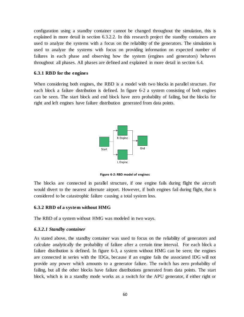
60

configuration using a standby container cannot be changed throughout the simulation, this is

explained in more detail in section 6.3.2.2. In this research project the standby containers are

used to analyze the systems with a focus on the reliability of the generators. The simulation is

used to analyze the systems with focus on providing information on expected number of

failures in each phase and observing how the system (engines and generators) behaves

throughout all phases. All phases are defined and explained in more detail in section 6.4.

6.3.1 RBD for the engines

When considering both engines, the RBD is a model with two blocks in parallel structure. For

each block a failure distribution is defined. In figure 6-2 a system consisting of both engines

can be seen. The start block and end block have zero probability of failing, but the blocks for

right and left engines have failure distribution generated from data points.

Figure 6-2: RBD model of engines

The blocks are connected in parallel structure, if one engine fails during flight the aircraft

would divert to the nearest alternate airport. However, if both engines fail during flight, that is

considered to be catastrophic failure causing a total system loss.

6.3.2 RBD of a system without HMG

The RBD of a system without HMG was modeled in two ways.

6.3.2.1 Standby container

As stated above, the standby container was used to focus on the reliability of generators and

calculate analytically the probability of failure after a certain time interval. For each block a

failure distribution is defined. In figure 6-3, a system without HMG can be seen; the engines

are connected in series with the IDGs, because if an engine fails the associated IDG will not

provide any power which amounts to a generator failure. The switch has zero probability of

failing, but all the other blocks have failure distributions generated from data points. The start

block, which is in a standby mode works as a switch for the APU generator, if either right or

61

left IDGs fails the start block is activated with certain probability, which activates the APU

generator if the start is successful.

Figure 6-3: RBD model of engines and generators in stand-by container

Number of active paths required for the system to be operating can be defined within the

standby container in BlockSim. If required paths are for example two, then one IDG can fail,

but if the APU doesn t start successfully the system is considered to have failed. If only one

path is required then the system would still be considered functioning although the APU

wouldn t start, all generators would have to fail for the system to fail.

6.3.2.2 Simulating RBD through different phases.

As stated above different system models were constructed to analyze a system that might

potentially have to divert from its original route to the nearest alternative airport. This is

because, the reliability-wise connection between components within the system changes if the

aircraft must be diverted. As it is not possible to implement this change within a stand-by

container, another model was constructed. To model the system, in such a way that it would

imitate the real-life behavior of the system, state change triggers (STC) and predefined groups

of blocks which trigger the STC were used. A SCT is an important and powerful feature in

BlockSim when modeling a complex system. State changes triggers in blocks make it possible

to specify events that will activate and/or deactivate the block during simulation. The initial

state of the block must be defined when the simulation starts, either as being on or off. All

blocks that might trigger state changes (active/deactivate) in other blocks throughout the

simulation, have to be clearly defined [22], [65]. This feature of BlockSim can only be used

when performing simulation and enables modeling of cold standby 30 configuration without

using a standby container.

30 Cold standby configuration is where the component cannot fail when it is in a standby mode [32]

62

In figure 6-4, an RBD of the engine and electrical system, which represents the reliability-wise

connection in a normal phase, can be seen. For the system to operate normally, i.e. so that the

aircraft would not have to be diverted from its original route, both engines need to be running

and at least two generators. State change triggers are represented with a blue quadrangle (in

lower right corner). If a block belongs to a predefined group that can trigger a state change it

has a red circle (in the upper left corner). The red circle in the right engine block is connected

to the blue STC in the right IDG block, meaning that if the right engine fails the right IDG

fails as well, but not vice versa. The same goes for the left engine block and the left IDG

block. The STC in the APU start block defines the block as inactive in the beginning, but is

activated if either the right or left IDG fails.

.

Figure 6-4: RBD model of the system in normal phase

If either one engine fails or if an IDG fails and the APU generator cannot be started, then the

aircraft would have to divert from its original route, to the nearest alternate airport. The RBD

in figure 6-5, shows how the reliability-wise connection changes. In a diversion at least one

engine needs to be running and at least one generator. Otherwise the system is considered to

have suffered a total failure.

63

Figure 6-5: RBD of the system in diversion phase

For each block in the RBD represented in figure 6-4 and 6-5 a failure distribution is defined.

The system start block has zero probability of failing. The circles represent how many

successful paths need to be functioning for the system to operate in that particular phase. The

circles themselves have zero probability of failing. The APU Start block has fixed probability

of success and ther blocks in the RBD have defined failure distribution generated from data

points.

6.3.3 RBD of a system with HMG

The RBD of a system with HMG was also modeled in two ways.

6.3.3.1 Standby container

For each block in the standby container, a failure distribution is defined. In figure 6-6 a system

with an HMG can be seen. This RBD is identical to the one for a system without an HMG,

except for one additional block which represents the HMG. The HMG is listed as a second

standby unit, meaning that the APU generator is a standby unit number one and is therefore

started before the HMG. In this standby container the APU start block also works as a switch,

with certain probability of starting successfully. However, the assumption is made that the

HMG will always be successfully started if needed. The switch itself (on the container)

therefore has zero probability of failing, but all the other blocks have failure distributions

generated from data points.

64

Figure 6-6: RBD model of engines and generators with HMG in Standby container

Due to the fact that the HMG is a second standby unit that cannot be activated unless all main

AC power has been lost, this model is analysed for when one active path is required. If the

system would be analyzed with two active paths as a requirement, then the software would

assume that the HMG could be started before all main AC power is lost.

6.3.3.2 Simulating RBD with HMG through different phases

In figure 6-7, an RBD of the system with HMG, which represent the reliability-wise

connection in a normal phase, can be seen. For the system to operate normally, i.e. so that the

aircraft would not have to go out of its original route, both engines need to be running and at

least two generators. The Block which represents the APU generator is inactive in the

beginning but is activated during the simulation if the right or left IDG fails. The block which

represents the HMG is also inactivated in the beginning but is activated during the simulation

if an APU start of the generator fails as well. Due to fact that it turned out to be difficult to

implement in the model, the assumption is made that if two generators are required (as in

normal phase) that the HMG can be started if two generators have failed. This is not possible

in reality; however it makes the system with an HMG more reliable than it actually is, but will

not affect the results of the system without an HMG. This is therefore a rather conservative

assumption, considering that results from models with and without an HMG will be compared.

65

Figure 6-7: RBD model of the system with HMG in normal phase

If either one engine fails or if and IDG fails and the APU generator cannot be started, then the

aircraft would have to divert from its original route, to the nearest alternate airport. The RBD

in figure 6-8, shows how the reliability-wise connection changes.

Figure 6-8: RBD of the system with HMG in diversion phase

For each block in the RBD represented in figure 6-7 and 6-8 a failure distribution is defined.

The start block has zero probability of failing. The circles represent how many successful

paths need to be functioning for the system to operate in that particular phase. The circles

themselves have also zero probability of failing. The APU start block has fixed probability of

success and other blocks in the RBD have defined failure distribution generated from data

points.

66

6.4 Reliability Phase Diagram (RPD)

The RPD is used to analyze the models through simulation with the BlockSim software. When

an RPD is being used as an extension of the RBD approach, it becomes possible to analyze

systems that might undergo changes in its reliability-wise configuration over its operating time

period [22],[32].

In a normal flight the aircraft goes through different phases during operation. These phases

are; taxi, take-off, climb, cruise, descent and landing and will all be implemented in the

models, except for the taxi phase. Only scenarios where the aircraft is airborne are being

analyzed and therefore the taxi phase is not included, since it is a ground phase. Different

stress loads between phases can be implemented in the BlockSim software. There are different

stress loads on aircrafts components depending on which phase it is operating in. However,

from the data collected for the making of this research project, it could not be estimated in

what phase components were when failure occurred. Therefore, stress loads between

components could not be implemented. The data would need to be much more detailed in

order to do so. This is, however, something that could be necessary to implement in the model

to obtain more reliable results and could therefore be an eligible project for future work.

If a failure occurs in-flight, i.e. a failure that would result in turn back to point of departure or

diversion to the nearest alternate airport then the reliability-wise configuration of the RBD

models changes. Consequently, other phases are needed to represent those changes in the

model. These phases are air turn back and diversion. If a failure occurs in either the take-off

phase or climb phase then it is assumed that the aircraft would enter an air turn back phase,

meaning that the aircraft would turn back to the departure airport. If a failure occurs in the

cruise phase then the aircraft would have to be diverted to the nearest alternate airport. If a

failure occurs in descent or landing then the reliability-wise connection of the RBD model

representing the aircraft would also change. The aircraft would however continue with the

landing at its original destination airport. This event will be represented with another phase in

the RPD, called emergency landing.

In the above situation, if a failure were to occur, i.e. such a failure that would lead to air turn

back, diversion or emergency landing, the failure is critical but would not be thought of as a

catastrophic failure leading to a total loss of the system. However, if a failure occurs in either

air turn back, diversion or emergency landing, these failures could cause a total loss of the

system. If for example one engine fails in the cruise phase and the aircraft must divert and the

other engine fails in the diversion phase this could lead a catastrophic accident. The duration

of each of these phases can be set as a constant in the BlockSim software. However, if a

failure occurs which would lead to a diversion, the software will stop simulating in that phase

and move to appropriate phase. When considering the duration of the flight to be simulated, it

67

must reflect actual duration of an ETOPS flight. Figure 6-9 shows a route from Keflavik to

Seattle, if the aircraft are non-ETOPS they cannot fly over the gray area, meaning that the

aircraft would have to take a longer route.

Figure 6-9: Route form Keflavik to Seattle - Non ETOPS [62]

In figure 6-10 the same route can be seen, but flown by an aircraft with 120 minutes ETOPS

approval. Here it can be seen that the gray area is gone, meaning that the aircraft could fly 120

minutes from the nearest alternate airport and therefore in this case the shortest route. This

route is an example of a scenario where it would be beneficial for Icelandair to operate with

120 minute ETOPS approval. The flight from Keflavík to Seattle is approximately 8 hours and

therefore that timeframe will be used in this analysis.

Figure 6-10: Route from Keflavik to Seattle - 120 minutes ETOPS approval [62]

68

Given that the duration of the flight is 8 hours and that models with different diversion times

are going to be compared, the estimated durations of the phases which will be used in the

simulation are represented in table 6-6.

Table 6-6: Duration of different phases

Phase Duration (Hours)

Take-off 0,1

Climb 0,4

Cruise 7

Descent 0,4

Landing 0,1

Air turn back 0,5

Diversion without HMG 2 (120 minutes) Diversion With HMG 3 (180 minutes)

Emergency Landing 0,5

When simulating the model with four electrical power sources (with an HMG), the duration of

the diversion phase, will be set to 180 minutes and when simulating with three electrical

power sources (without an HMG), the duration of the diversion phase will be 120 minutes. If a

failure occurs in either diversion phases, at some time, the simulation will stop; it will not

finish the time remaining time in that phase.

6.4.1 The RPD model

The resulting RPD which will be used to simulate the 8 hour flight can be seen in figure 6-11.

Figure 6-11: RPD used to simulate systems

69

The green lines in the RPD represent the success path whereas the red lines represent the

failure paths. After a successful operation in take-off the simulation moves on to climb phase,

if climb phase operates successfully the simulation moves on to cruise phase and so on. If a

critical failure occurs in; take-off, climb-, cruise, descent or landing the simulation will move

on to either air turn back, diversion or emergency landing, whichever is relevant at that state.

If a failure occurs in those phases the simulation will move on to a stop block, representing a

total loss of the system. The simulation stops and starts a new simulation from the beginning.

The node is used to represents cases where the aircraft manages to land safely, whether it’s a

success path leading from landing phase, air turn back, diversion or emergency landing. After

a safe landing the simulation ends and a new one begins.

71

7. RESULTS AND DISCUSSIONS

In the previous chapter Reliability Block Diagram (RBD) models of the systems and a

Reliability Phase Diagram (RPD) were developed including a discussion of the reliability-wise

configuration of subsystems and components in the system models. Models for the failure

behavior of each block in the system model were also defined by analyzing operational data

obtained from Icelandair, Delta Airlines and Rolls-Royce.

In this chapter the reliability models developed in previous chapters will be used to calculate

the reliability for the systems with the primary objective of determining the capability of the

electrical power system to satisfy reliability requirements for ETOPS operations. The systems

are analyzed both analytically and through simulation and reliability results will be discussed,

with the aim of answering research questions 1-5 which were presented in section 1.4, they are

the following;

1. What is the reliability of the electrical system in question?

2. Are all requirements listed in section 1.2, fulfilled for a system without an HMG?

3. What is the probability of failure of a system with three generators with maximum

diversion time of 120 minutes compared to a system with an HMG installed as the

fourth generator with approved maximum diversion time of 180 minutes? Is there a

significant difference?



generators?


determine the overall reliability of the systems?

Research question 6, concerning future work, will be answered in chapter 8.

The requirements and objectives listed in section 1.2 are the following;

In-flight start reliability of the APU should not be less than 95%

In-flight engine shut-down (IFSD) rate needs to be equal to or less than 0.027

shutdowns per 1000 engine flight hours.






72


Aeroplanes (CS-25) and can be found in references such as [13].

7.1 In-flight start of APU

Data concerning In-flight start of APU were analyzed and the average calculated as a 12-

month rolling average, which can be seen in figure 7-1.

Figure 7-1: Data on APU In-flight start, represented on a 12-month rolling average base.

The requirements listed in section 1.2 specify that the In-flight start reliability of the APU

should not be less than 95%. According to Deltas Airlines data the probability of a

successful in-flight start of the APU (or reliability) has never gone below 95% over the last

three years and the average of 12 month rolling average over the period from September 2013

to August 2016 is 99 %, which is well above the requirements of a 95% in–flight start

reliability of the APU.

7.2 IFSD rate

The requirements listed in section 1.2 also specify that the In-flight shut-down (IFSD) rate

needs to be equal to or less than 0,027 shutdowns per 1000 engine flight hours. Data

collected from Rolls-Royce only included information on the RB211-535E4/B engine types,

which are the same engine types as Icelandair operates. According to the data total engine

hours on a world fleet basis were 14.416.475 hours. Number of IFSD over the same period

95%

96%

96%

97%

97%

98%

98%

99%

99%

100%

100%

Pro

ba

bilit

y

Month

Probability of a successfull APU In-flight start -12 Month rolling average-

73

were 91, therefore the number of IFSD per flight hour is 0,0000063122 or 0,0063122 IFSD

per 1000 flight hours , which is well below the requirement of 0,027 IFSD per 1000 flight

hours. Also, according to Boeing s ETOPS quarterly report 2014, the published 12 month

rolling IFSD rate is 0,008 engine shutdowns per 1000 engine flight hours [43]. Consequently it

has already been demonstrated that the RBD211-535 engine is reliable enough and fulfills

ETOPS requirements by a significant margin.

7.3 Engines

The requirements listed in section 1.2 also specify that the probability of a catastrophic

accident due to complete loss of thrust from independent causes must be no worse than

0,3 x 10-8 per flying hour. To calculate the engine reliability and probability of a dual engine

shutdown, both analytical calculations and simulation were performed.

7.3.1 Analytical calculations

With analytical calculations the exact mathematical expression was used to calculate the

reliability with t = 8 hrs, which would correspond to a flight duration from Keflavík to

Seattle31.

To calculate the reliability of a system consisting of two engines in parallel structure, the

following mathematical expression was used;

𝑅𝑠(𝑡) = 1 − (1 − ∫ 𝑓(𝑥)𝑅𝐸𝑛𝑔𝑖𝑛𝑒𝑑𝑥∞

𝑡

) (1 − ∫ 𝑓(𝑥)𝐿𝐸𝑛𝑔𝑖𝑛𝑒𝑑𝑥∞

𝑡

)

The distribution that was chosen32 to describe the failure behavior of engines, with regard to

IFSD, was the exponential distribution with mean time to failure of 160.115 engine hours on

world fleet basis and a constant failure rate λ = 0,625 ∗ 10−5 failures/hr.

𝑅𝑠(𝑡) = 1 − (1 − ∫ 𝑓(𝑥)𝑅𝐸𝑛𝑔𝑖𝑛𝑒𝑑𝑥∞

𝑡

) (1 − ∫ 𝑓(𝑥)𝐿𝐸𝑛𝑔𝑖𝑛𝑒𝑑𝑥∞

𝑡

)

𝑅𝑠(𝑡) = 1 − (1 − ∫ 𝜆𝑒−𝜆𝑥 𝑑𝑥∞

𝑡

)(1 − ∫ 𝜆𝑒−𝜆𝑥 𝑑𝑥∞

𝑡

)

𝑅𝑠(𝑡) = 1 − (1 − 𝑒 −𝜆𝑡)(1 − 𝑒−𝜆𝑡)

31 The fl ight route which was chosen is discussed in more detail in section 6.4. 32 See section 6.2.1.2 for further information.

74

Thus the reliability of two engines with t = 8 hrs. is;

𝑅𝑠(8) = 1 − (1 − 𝑒−0,0000062455𝑡)(1 − 𝑒−0,0000062455𝑡) = 0,9999999975

Consequently, the probability of a dual engine failure during an 8 hr. flight is;

𝑄(𝑡) = 1 − 𝑅(𝑡)

𝑄(8) = 1 − 0,9999999975 = 𝟎, 𝟐𝟓 ∗ 𝟏𝟎−𝟖

This however is the probability of a dual engine failure during an 8 hour flight, which would

equal to 𝟎, 𝟑𝟏𝟑 ∗ 𝟏𝟎−𝟗 probability of dual engine failure per flying hour. This is well

below the requirement of 𝟎, 𝟑 ∗ 𝟏𝟎−𝟖 per flying hour as stated in the ETOPS

requirements .

7.3.2 Simulation

The system consisting of two engines in a parallel structure was simulated in two ways. First

only the RBD was simulated, as if the flight consisted of only one phase with duration of 8

hours. Results obtained, should be similar to the results from analytical calculations. The RPD

approach was then used to model all phases (i.e. take-off, climb, cruise, descent, landing,

emergency landing, diversion and air turn back), allowing changes in the reliability-wise

configuration of the system to be modeled and simulated.

7.3.2.1 Simulation of RBD

The system of two engines connected reliability-wise in parallel was simulated 1.000.000

times. Each simulation run was 8 hours, so that in total the simulation generates 8.000.000

flight hours and hence 16.000.000 engine hours.

Table 7-1: Simulation results after simulating system with two engines 1.000.000 times.

System Overall Results

Mean Availability (All Events): 100%

Std. Deviation (Mean Availability): 0

Reliability at 8 hours (prob. of no failure): 100%

Expected Number of Failures: 0

Std. Deviation (Number of Failures): 0

Individual Block Information: Right and Left Engine

Mean Availability (All Events): 0,999973

Expected Number of Failures: 0,000053

Mean Time Between Failure 150.939

75

The results in table 7-1 are obtained as the average of the results over all simulations. For the

overall system the mean availability and reliability is 100%, which means that over all

simulations there was never a dual engine failure. This however does not reflect the reality;

the reliability of the system is not 100%. This only indicates that there was never a dual engine

failure over these 16.000.000 engine hours. A dual engine failure would have been more likely

to occur in simulation if the system would have been simulated over, for example, 10.000.000

flights (i.e. 160.000.000 engine hours), as the probability of such an event is extremely low.

For the engines individually, the mean availability or reliability is 99,9973 %, expected

number of failures is 0,000053 for each engine over a 8 hour flight which would result in 106

IFSD s over 8.000.000 flight hours or 16.000.000 engine hours. Consequently, the IFSD rate

would be equal to 106/16.000.000 per engine hour, which equals 0,006625 per 1000 engine

hours. The mean time between IFSD is 150.939 engine hours, which is less than estimated

from when using the exponential distribution. But still, the simulation results show that

simulating the system over 16.000.000 engine hours generates results that are in line with data

obtained from Rolls-Royce. The simulation, based on the engine reliability model, gives

results that are in good agreement with the data which was used to develop the model (i.e. the

chosen lifetime distribution).

Using the mathematical model, used in the analytical calculation, combined with results for a

single engine shut down from the simulation the reliability of the overall system can be

calculated. With λ=1/150939 failures/hr. the reliability can be calculated as;

Rs(8) = 1 − (1 − e−( 1

150939)∗8)(1 − e

−( 1150939

)∗8) = 0,9999999972

Consequently, the probability of a dual engine failure can be calculated as;

Q(8) = 1 − 0,9999999972 = 0,28 ∗ 10−8

This however is also the probability of a dual engine failure over an 8 hour flight, which

would equal to 𝟎, 𝟑𝟓 ∗ 𝟏𝟎−𝟗 probability of a dual engine failure per flight hour. Which is

well below the requirement of 𝟎, 𝟑 ∗ 𝟏𝟎−𝟖 per flying hour as stated in the ETOPS

requirements.

Results obtained from analytical calculations and results obtained by using parameters

generated from simulation are very similar, i.e. the difference is small. With even more

simulations, the convergence of the results would increase further. The purpose for calculating

the reliability of engines both with analytical calculations and by simulation was mainly to

validate the use of the BlockSim software, whereby the software performs all computation

regarding generators and overall systems reliability.

76

7.3.2.2 Simulation using RPD

The Reliability Phase Diagram (RPD) was also applied in order to achieve 1.000.000 flights

with each flight set to 8 hours. This generates 16.000.000 engine hours. However, as explained

in the previous subsection, orders of magnitude more simulation runs would have to be run in

order for a dual engine failure to occur as such a system state has a very low probability of

occurring. The duration of the diversion phase33 was set to 120 minutes. Each phase in the

diagram has a fixed time throughout all simulations, however if a failure occurs, leading to

diversion, air turnback or emergency landing, the simulation will end it s current phase and

move to appropriate phase.

Table 7-2: Frequency of single engine failures in each phase, results from simulating the RPD.

Frequency of single engine failures

Phases

Take-off 0,000002

Climb 0,000007

Cruise 0,000093

Descent 0,000008

Landing 0

Diversion 0

Air turn back 0

Emergency landing 0

Total 0,00011

Results from simulating the RPD can be seen in table 7-2 (and graphically in figure 7-2). Total

number of failures in all phases is equal to 0,00011, which results in 110 IFSD over all

1.000.000 flights. In Take-off phase the frequency of IFSD is 0,000002. Frequency of IFSD is

0,000007 in Climb phase, 0,000093 in Cruise phase and 0,000008 in Descent phase. In other

phases, i.e. Landing, Diversion, Air turn-back and Emergency landing the expected failure is

equal to 0, meaning that through all simulation there was never a dual engine shut down. From

the above results, the IFSD rate would be equal to 110/16.000.000 per engine hour, which

equals to 0,006867 IFSD per 1000 engine hours and the mean time between IFSD is 145.455

engine hours.

33 Durations for phases is discussed in section 6.4.

77

Figure 7-2: Frequency of single engine failures in each phase, results from simulating the RPD

In figure 7-2, the frequency of failures in each phase can be seen. Phases are listed on the x-

axis and the y-axis represents the expected number of failures in each phase.

Simulating the RPD can give, among other things, useful information on the number of IFSDs

in different phases. However, due to the fact that different stress loads were not implemented

in the model, the number of IFSDs in each phase is largely dependent on the duration of the

phases. Consecuently, the cruise phase has the highest number of failures as its duration is the

longest. According to ITS Powerplant Engineer34 the stress load on the engines is highest in

both take-off and climb phase. Therefore, the results obtained by simulating the RPD, do not

give usefull or reliable information. In order to obtain reliable results from when simulating

the RPD, it is necessary to implement different stress loads between phases.

34 Hafdís Ósk Pétursdóttir

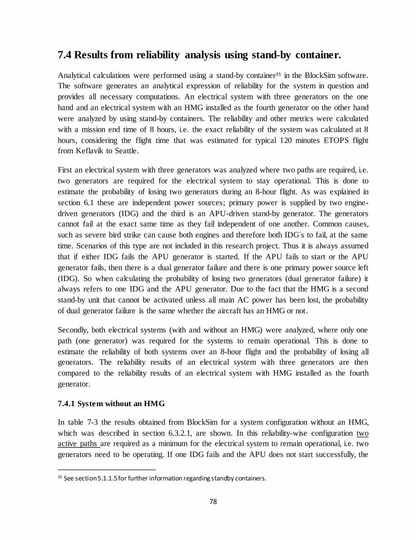
78

7.4 Results from reliability analysis using stand-by container.

Analytical calculations were performed using a stand-by container35 in the BlockSim software.

The software generates an analytical expression of reliability for the system in question and

provides all necessary computations. An electrical system with three generators on the one

hand and an electrical system with an HMG installed as the fourth generator on the other hand

were analyzed by using stand-by containers. The reliability and other metrics were calculated

with a mission end time of 8 hours, i.e. the exact reliability of the system was calculated at 8

hours, considering the flight time that was estimated for typical 120 minutes ETOPS flight

from Keflavík to Seattle.

First an electrical system with three generators was analyzed where two paths are required, i.e.

two generators are required for the electrical system to stay operational. This is done to

estimate the probability of losing two generators during an 8-hour flight. As was explained in

section 6.1 these are independent power sources; primary power is supplied by two engine-

driven generators (IDG) and the third is an APU-driven stand-by generator. The generators

cannot fail at the exact same time as they fail independent of one another. Common causes,

such as severe bird strike can cause both engines and therefore both IDG s to fail, at the same

time. Scenarios of this type are not included in this research project. Thus it is always assumed

that if either IDG fails the APU generator is started. If the APU fails to start or the APU

generator fails, then there is a dual generator failure and there is one primary power source left

(IDG). So when calculating the probability of losing two generators (dual generator failure) it

always refers to one IDG and the APU generator. Due to the fact that the HMG is a second

stand-by unit that cannot be activated unless all main AC power has been lost, the probability

of dual generator failure is the same whether the aircraft has an HMG or not.

Secondly, both electrical systems (with and without an HMG) were analyzed, where only one

path (one generator) was required for the systems to remain operational. This is done to

estimate the reliability of both systems over an 8-hour flight and the probability of losing all

generators. The reliability results of an electrical system with three generators are then

compared to the reliability results of an electrical system with HMG installed as the fourth

generator.

7.4.1 System without an HMG

In table 7-3 the results obtained from BlockSim for a system configuration without an HMG,

which was described in section 6.3.2.1, are shown. In this reliability-wise configuration two

active paths are required as a minimum for the electrical system to remain operational, i.e. two

generators need to be operating. If one IDG fails and the APU does not start successfully, the

35 See section 5.1.1.5 for further information regarding standby containers.

79

system is defined to have failed. The IDG can either fail due to engine failure or due to

internal failure of the IDG itself. The estimated probability of a successful start of the APU is

99%36. After a successful APU start, the APU itself will not fail, however the APU generator

can still fail. Here, the main goal is to estimate the probability of losing two generators during

an 8-hour flight.

Table 7-3: Reliability results for a system with three generators in

a stand-by container where two paths are required.

System results with three generators for an 8-hour flight

Reliability: 0,9999875

Prob. of Failure: 1,25E-05

Failure Rate (/Hr.): 1,73E-06

Mean Life (Hrs.) 10.466

From the results in table 7-3 it can be seen that the reliability at 8 hours is 99,99875 % and the

probability of failure is 1,25 ∗ 10−5. The average failure rate is 1,73 ∗ 10−6 per hour and the

mean life (or the mean time to failure (MTTF)) is 10.466 hours. In figure 7-3 a plot of the

reliability function over an 8-hour flight, can be seen. The y-axis represents the reliability on

the scale from 0,9999 to 1 and the x-axis represents the timeline from 0 to 8 hours.

36 See section 6.2.5 for further information on estimation of the APU in-fl ight start.

80

Figure 7-3: Reliability function; system with three generators where two active paths are required.

One of the requirements listed in section 1.2 is that the probability of losing two out of three

electrical power sources should meet the safety objective of being less than or on the

order of 10-5 per flying hour, which is defined as probability of a major failure condition

(see reference [13]). The results for an electrical system with three generators, where two

paths are required for the system remain operational can be used to estimate the probability of

losing two generators. The reliability is 99,99875 % and probability of failure is 1,25 ∗ 10−5

for an 8-hour flight. The average failure rate was estimated to be 1,73 ∗ 10−6 per flying hour.

According to these results, an electrical system with three generators (without an HMG)

exceeds this safety objective by almost one order of magnitude.

In table 7-4 the results for a system configuration without an HMG can be seen, with the same

assumption as before except that now only one active path is required as a minimum for the

system to remain operational, i.e. only one generator needs to be operating. The main goal is

to estimate the probability of losing all three generators during an 8-hour flight.

81

Table 7-4: Reliability results for a system with three generators in a stand-by container where one path is required.

System results with three generators for an 8-hour flight

Reliability: 0,99999999666




The reliability for the system at 8 hours is 99,999999666 % and the probability of failure is

3,34 ∗ 10−9. The average failure rate is 8,58 ∗ 10−10 per flying hour and the mean life

(MTTF) is 25.750 hours. A plot of the reliability function for an 8-hour flight can be seen in

figure 7-4. The reliability increases when only one path is required for the system to stay

operational, therefore the y-axis which represents the reliability was now plotted from

0,99999999 to 1.

Figure 7-4: Reliability function; system with three generators where one active path is required.

82

Research question 1: What is the overall reliability of the electrical system in question?

The results for an electrical system with three generators, where one path (one generator) is

required for the system to remain operational, express the overall reliability and probability of

losing all three generators during an 8-hour flight. According to the results, the overall

reliability for an electrical system with three generators for an 8-hour flight is

99,999999666 % and probability of failure is 𝟑, 𝟑𝟒 ∗ 𝟏𝟎−𝟗. The average failure rate is

estimated to be 𝟖, 𝟓𝟖 ∗ 𝟏𝟎−𝟏𝟎 per flying hour. Thus the first research question has been

answered with regard to an electrical system with three generators.

Research question 2: Are all requirements listed in section 1.2, fulfilled for an electrical

system without an HMG?

The requirements and objectives listed in section 1.2 are the following;

In-flight start reliability of the APU should not be less than 95%

In-flight engine shut-down (IFSD) rate needs to be equal to or less than 0.027

shutdowns per 1000 engine flight hours.







Aeroplanes (CS-25) and can be found in reference such as [13].

Calculations in the above sections show that;

The reliability of the APU in-flight start is 99% (see section 7.1).

The IFSD rate is 0,0063122 per 1000 flight hours (see section 7.2).

The probability of dual engine failure is 0,313 ∗ 10−9 per flying hour (see section

7.3).

The probability of losing two electrical power sources during an 8-hour flight is on

average 1,73 ∗ 10−6 per flying hour (see section 7.4.1)

After analyzing the results for an electrical system with three generators (without an

HMG) the results show that all requirements listed in section 1.2 are fulfilled. Thus

research question number two has been answered.

83

7.4.2 System with an HMG

The HMG is a second stand-by unit that is not activated unless all main AC power has been

lost; the probability of losing one IDG and the APU generator is the same whether the aircraft

has an HMG or not. Therefore, the probability of dual generator failure is the same for these

systems.

As for an electrical system with three generators the stand-by container can be used to

calculate the probability of losing all four generators in an electrical system with an HMG. In

table 7-5 the results for a system configuration with an HMG, which was described in section

6.3.3.1, are shown for an 8-hour flight. In this reliability-wise configuration only one active

path is required as a minimum for the system to remain operational, i.e. one generator needs to

be operating.

Table 7-5: Reliability results for a system with four generators in

a stand-by container where one path is required

System results with four generators for an 8-hour flight

Reliability: 0,9999999999978




The reliability for the system at 8 hours is 99,99999999978 % and the probability of failure

is 2,15 ∗ 10−12. The average failure rate is 8,39 ∗ 10−13 per flying hour and the mean life is

26.193 hours. In figure 7-5 a plot of the reliability function for an 8-hour flight, can be seen.

Here, the y-axis represents the reliability on the scale from 0,999999999 to 1.

84

Figure 7-5: Reliability function; system with four generators where one active path is required.

Research question 1: What is the overall reliability of the electrical system in question?

The results for an electrical system with four generators, where one path (one generator) is

required for the system to remain operational, express the overall reliability and probability of

losing all four generators during an 8-hour flight. According to the results, the reliability for

an electrical system with four generators for an 8-hour flight is 99,99999999978 % and

probability of failure is 𝟐, 𝟏𝟓 ∗ 𝟏𝟎−𝟏𝟐. The average failure rate is estimated to be 𝟖, 𝟑𝟗 ∗

𝟏𝟎−𝟏𝟑 per flying hour. Thus research question one has been answered with regard to an

electrical system with four generators, i.e. the HMG installed as the fourth.

85

7.4.3 Comparison of results for a systems with and without HMG

In table 7-6, a comparison of main results for systems with and without an HMG at 8 hours

can be seen.

Table 7-6: Comparison of systems results where one generator is required as a minimum during an 8 -hour flight.

Comparison of systems

with three generators (NO HMG)

with four generators (with HMG)

Reliability: 0, 99999999666 0,9999999999978

Prob. of Failure: 3,34E-09 2,15E-12

Failure Rate (/Hr.): 8,58E-10 8,39E-13

As can be seen from the table the difference in probability of failure, for the two types of

system is significant. This difference is expected due to higher redundancy obtained with the

installation of the HMG. However, it should be noted that it is assumed that the HMG would

have similar failure distribution as the APU generator. As explained in section 6.1, the APU is

the primary standby power source that is started as soon as one of the primaries (IDG) fails.

Consequently it is used much more frequently than the HMG. It is also capable of powering

all critical aircraft systems as the APU has an order of magnitude more output than the HMG.

Attributing the same reliability to the HMG as the APU must be considered conservative in

favor of estimating its contribution to overall system reliability. Is is also assumed that the

HMG will always starts successfully, which increases the reliability of that system.

It is important to note that the difference in probability of losing all three generators and the

probability of a dual engine failure is insignificant. One of the requirements listed in section

1.2 was that the probability of losing thrust in both engines should be shown to be less than 0.3

x 10-8 per flying hour, which was shown to be 0,313 ∗ 10−9 (equivalent to 3,13 * 10-10) per

flying hour in section 7.3.1 based on data provided by the manufacturer of RB-211 engines.

These results indicate that it is as likely that a catastrophic accident will occur due to a dual

engine failure as due to a total loss of all AC power even if only three generators are installed.

It can therefore be concluded that the installation of the HMG is superfluous. Moreover, as

mentioned in section 6.1.1 (and can bee seen in electrical block diagram in appendix D) if

electrical system without HMG loses all main AC power, the main battery will supply back-up

power to flight critical loads for a certain amount of time, usually 30 to 60 minutes, depending

on the battery. This was not implemented in the model, but would further enhance the

reliability of the electrical system.

86

In figure 7-6 the reliability functions for both types of AC electrical systems are plotted over

an 8-hour flight. The blue line represents an electrical system with three generators and the

green line represents an electrical system with an HMG installed as the four generator. Here,

the y-axis represents the reliability on the scale from 0,99999999 to 1.

Figure 7-6: Reliability functions; both systems where one generator is required as a minimum.

7.5 Diversion due to different failure modes

In this section different failure modes which would have the most critical effect on the

electrical system and result in immediate diversion to the nearest alternate airport, are

considered. The probability of such an event to occur is estimated for predefined point of time.

Following this event, both types of electrical systems, i.e. with and without an HMG, are

analyzed over a period equivalent to either a two or three hour diversion time depending on

the system. Thus an electrical system with an HMG is analyzed for a diversion time of three

hours and an electrical system without an HMG is analyzed for a diversion time of two hours.

Here the objectives are to estimate the probability of a total AC power failure for both systems

87

in diversion phase following a predefined failure that lead to the diversion and to compare the

systems.

There are two failure modes that lead to an immediate diversion and have a major impact on

the electrical system, they are;

1. Single engine failure

2. Dual generator failure (one IDG fails and the APU fails to start or APU generator fails

after it is started)

The aircraft must always be diverted when a single engine failure occurs. Such a failure also

affects the electrical systems, wherein the IDG s are engine driven generators, so that if one

engine fails the associated IDG fails as well. The IDG can however fail without the engine

failing, but not vice versa. In situations where one IDG fails (without an engine failure) and

the APU cannot be started or if the APU generator fails after a successful APU start, then a

dual generator failure has occurred. In such situations the aircraft must also always be diverted

to the nearest alternate airport, whether the aircraft has an HMG installed as the fourth

generator or not.

The assumption is made that component failures are independent from each other, both IDG s

cannot fail at the same time and both engines cannot either fail at the same time, as was

explained in section 7.4.

7.5.1 Diversion due to a single engine failure

The probability of a single engine failure is the same, whether the aircraft has an HMG or not.

A model of two engines was presented in chapter 6.3.1, however, now the assumption is made

that both engines need to be operating for the system, consisting only of engines, to be

functioning. Therefore, if one engine fails the system is defined to have failed as well. With

this assumption the probability of losing one engine can be calculated as if the engines were

connected reliability-wise in series37.

As estimated in chapter 6.2.1.2, the exponential distribution with a constant failure rate of

0,625∗ 10−5 per hour can be used to describe the failure behavior of the engines. The

reliability and probability of a single engine failure was calculated at time t = 6 hours. This

could have been calculated for any time period, however the 6 hour flying time was chosen

because in a typical flight from Keflavík to Seattle the aircraft would be in the middle of an

ETOPS segment at this point in the flight (see figure 6-9 in section 6.4)

37 See section 5.1.1.1 for further information on RBD in series configuration.

88

The following mathematical expression was used to calculate the reliability;

𝑅𝑠(𝑡) = (∫ 𝑓(𝑥)𝑅𝐸𝑛𝑔𝑖𝑛𝑒𝑑𝑥∞

𝑡

) (∫ 𝑓(𝑥)𝐿𝐸𝑛𝑔𝑖𝑛𝑒𝑑𝑥∞

𝑡

)

𝑅𝑠(𝑡) = 𝑒−𝜆𝑡 ∗ 𝑒−𝜆𝑡

Thus the reliability of the system with t = 6 hours is;

𝑅𝑠(6) = 𝑒−0,00000625∗6 ∗ 𝑒−0,00000625 = 0,999925057

Consequently, the probability of a single engine failure during a 6 hour flight is;

𝑄(𝑡) = 1 − 𝑅(𝑡)

𝑄(6) = 1 − 0,999925057 = 7,49 ∗ 10−5

The probability of a single engine failure during the first 6 hours of the flight is therefore

estimated to be 𝟕, 𝟒𝟗 ∗ 𝟏𝟎−𝟓 and as stated above this is the same, whether the aircraft has an

HMG or not.

Following a failure such as single engine failure that leads to diversion, it is assumed that an

aircraft without an HMG would be capable of diverting for 2 hours and that an aircraft with an

HMG would be capable of diverting for 3 hours. This is done to compare the electrical system

capabilities when they both are required to demonstrate their maximum diversion time. In

reality it is very unlikely that they are exactly at that point in the flight that they would have to

use their maximum diversion time. Furthermore, if flying the same route, aircraft with and

without HMG would both divert to the same alternate airport. However for the purpose of this

research project it is assumed that maximum diversion time is needed for both electrical

systems.

The BlockSim software was used to undertake all computations, by using stand-by containers

for an electrical system with an HMG and without an HMG, as described in chapters 6.3.2.1

and 6.3.3.1. In both RBD models the right IDG and the right engine were set as failed and only

one active path (one generator) was required for the system to remain operational. For an

electrical system without an HMG the results were analyzed from time 6 to 8 hrs., as if a

failure occurred at t = 6 and the aircraft had to be diverted for 2 hours. For an electrical system

with an HMG the results were analyzed from time 6 to 9, as if a failure occurred at t = 6 and

the aircraft had to be diverted for 3 hours.

89

Table 7-7: Comparison of systems with and without an HMG, both diverting due to a single engine failure.


With three generators diverting for 2 hours

with four generators diverting for 3 hours

Reliability: 0,99999838 0,99999999584


In table 7-7, the results show that for an electrical system with three generators, diverting due

to a single engine failure, that the reliability of the electrical system for 2 hours from 6 to 8

hours is 99,999838 % and the probability of failure over that 2 hour diversion period is 1,62 ∗

10−6. The results show that for an electrical system with four generators, that the reliability

for three hours from 6 to 9 hours is 99,999999584 % and the probability of failure over that

three hour diversion is 4,16 ∗ 10−9.

As the right and left engine have the exact same failure distribution and parameters, and

because both IDGs have the same failure distribution and parameters, these results are the

same whether considering right or left engine failure. Accordingly, if an aircraft has to divert

due to an engine failure an electrical system with an HMG has a significantly higher reliability

at the end of a 180 minutes diversion than a system without an HMG at the end of a 120

minutes diversion time.

Research question 3: What is the probability of losing all main AC power for an electrical

system with three generators with maximum diversion time of 120 minutes compared to an

electrical system with an HMG installed as the fourth generator with approved maximum

diversion time of 180 minutes? Is there a significant difference?

This research question will be answered based on two scenarios. First, the probability of a

total AC power loss in diversion phase, following a single engine failure that caused the

diversion. Secondly, the probability of a total AC power loss in diversion phase, following a

dual generator failure that caused the diversion. In both scenarios it is assumed that a failure

leading to diversion occurs at the first 6 hours of the flight, and that diversion time is either 2

or 3 hours, depending on the system in question.

For both systems (with and without an HMG) the probability of a single engine failure over 6

hours was estimated to be 7,49 ∗ 10−5. The probability of a failure over a 2 hour diversion

was estimated to be 1,62 ∗ 10−6 for an electrical system with three generators. The probability

of a failure over a 3 hour diversion was estimated to be 4,16 ∗ 10−9 for an electrical system

with the HMG installed as the fourth generator.

To calculate the exact probability for such an event to occur, i.e. single engine failure and a

total loss of the remaining generators in diversion, conditional probabilities can be used.

90

Assuming that failures are independent, following mathematical expression is used to

calculate the probability of total AC power loss;

𝑃(𝑇𝑜𝑡𝑎𝑙 𝐴𝐶 𝑝𝑜𝑤𝑒𝑟 𝑙𝑜𝑠𝑠)

= 𝑃(𝑆𝑖𝑛𝑔𝑙𝑒 𝑒𝑛𝑔𝑖𝑛𝑒 𝑓𝑎𝑖𝑙𝑢𝑟𝑒) ∗ 𝑃(𝐹𝑎𝑖𝑙𝑢𝑟𝑒 𝑖𝑛 𝑎 𝑑𝑖𝑣𝑒𝑟𝑠𝑖𝑜𝑛 𝑝ℎ𝑎𝑠𝑒)

Then for an electrical system without an HMG;

𝑃(𝑇𝑜𝑡𝑎𝑙 𝐴𝐶 𝑝𝑜𝑤𝑒𝑟 𝑙𝑜𝑠𝑠) = 7,49 ∗ 10−5 ∗ 1,62 ∗ 10−6 = 𝟏, 𝟐𝟐 ∗ 𝟏𝟎−𝟏𝟎

This is the estimated probability of a total AC power loss, for this exact event for an electrical

system without an HMG, which corresponds to approximately 𝟏, 𝟓𝟐 ∗ 𝟏𝟎−𝟏𝟏 per flying

hour.

Then for an electrical system with an HMG;

𝑃(𝑇𝑜𝑡𝑎𝑙 𝐴𝐶 𝑝𝑜𝑤𝑒𝑟 𝑙𝑜𝑠𝑠) = 7,49 ∗ 10−5 ∗ 4,16 ∗ 10−9 = 𝟑, 𝟏𝟐 ∗ 𝟏𝟎−𝟏𝟑

This is the probability of a total AC power loss, for this exact event for an electrical system

with an HMG, which corresponds too approximately 𝟑, 𝟒𝟕 ∗ 𝟏𝟎−𝟏𝟒 per flying hour.

When considering the safety objectives in Certification Specifications for Large Aeroplanes

(CS-25), extremely improbable failure conditions are defined as being less than or on the order

of 10−9 per flying hour [13]. Both electrical systems (with and without an HMG) exceed this

safety objective, therefore, it can be said that it is extremely improbable that either of these

events will occur.

Based on these results, it can be seen that there is a significant difference between an electrical

system with three generators and an electrical system with an HMG installed as the fourth

generator, when considering total AC power loss in diversion following a single engine

failure. The probability for an electrical system with an HMG to lose all AC power is

approximately three orders of magnitude lower than for an electrical system without an HMG,

despite being diverted for a longer time. However, as mentioned in section 7.4.3, attributing

the same reliability to the HMG as the APU is considered conservative in favor of estimating

its contribution to overall system reliability. Furthermore, it is assumed that the HMG will

always start successfully. If the HMG would have the same probability of a successful start as

the APU, the difference between the systems would reduce.

Thus research question number three has been answered with respect to single engine failure,

both for an electrical system without HMG and with an HMG.

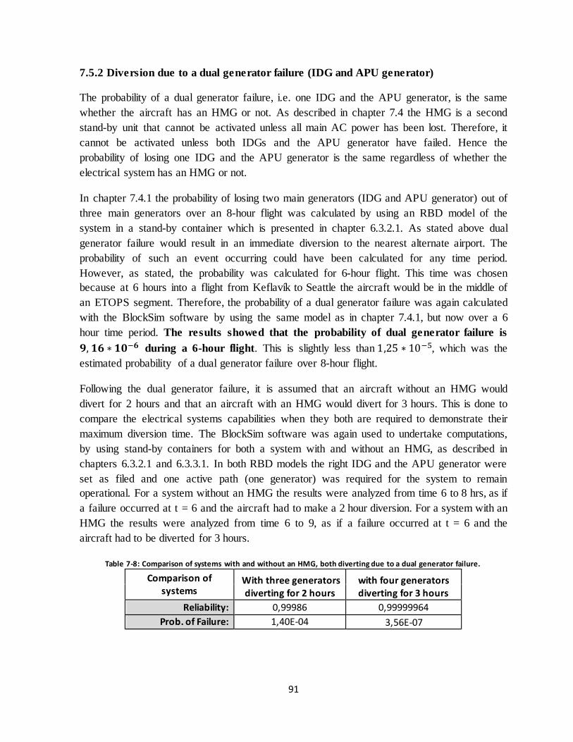
91

7.5.2 Diversion due to a dual generator failure (IDG and APU generator)

The probability of a dual generator failure, i.e. one IDG and the APU generator, is the same

whether the aircraft has an HMG or not. As described in chapter 7.4 the HMG is a second

stand-by unit that cannot be activated unless all main AC power has been lost. Therefore, it

cannot be activated unless both IDGs and the APU generator have failed. Hence the

probability of losing one IDG and the APU generator is the same regardless of whether the

electrical system has an HMG or not.

In chapter 7.4.1 the probability of losing two main generators (IDG and APU generator) out of

three main generators over an 8-hour flight was calculated by using an RBD model of the

system in a stand-by container which is presented in chapter 6.3.2.1. As stated above dual

generator failure would result in an immediate diversion to the nearest alternate airport. The

probability of such an event occurring could have been calculated for any time period.

However, as stated, the probability was calculated for 6-hour flight. This time was chosen

because at 6 hours into a flight from Keflavík to Seattle the aircraft would be in the middle of

an ETOPS segment. Therefore, the probability of a dual generator failure was again calculated

with the BlockSim software by using the same model as in chapter 7.4.1, but now over a 6

hour time period. The results showed that the probability of dual generator failure is

𝟗, 𝟏𝟔 ∗ 𝟏𝟎−𝟔 during a 6-hour flight. This is slightly less than 1,25 ∗ 10−5, which was the

estimated probability of a dual generator failure over 8-hour flight.

Following the dual generator failure, it is assumed that an aircraft without an HMG would

divert for 2 hours and that an aircraft with an HMG would divert for 3 hours. This is done to

compare the electrical systems capabilities when they both are required to demonstrate their

maximum diversion time. The BlockSim software was again used to undertake computations,

by using stand-by containers for both a system with and without an HMG, as described in

chapters 6.3.2.1 and 6.3.3.1. In both RBD models the right IDG and the APU generator were

set as filed and one active path (one generator) was required for the system to remain

operational. For a system without an HMG the results were analyzed from time 6 to 8 hrs, as if

a failure occurred at t = 6 and the aircraft had to make a 2 hour diversion. For a system with an

HMG the results were analyzed from time 6 to 9, as if a failure occurred at t = 6 and the

aircraft had to be diverted for 3 hours.

Table 7-8: Comparison of systems with and without an HMG, both diverting due to a dual generator failure.


With three generators diverting for 2 hours

with four generators diverting for 3 hours

Reliability: 0,99986 0,99999964


92

In table 7-8, the results show that for an electrical system with three generators, diverting due

to a dual generator failure, that the reliability of the system for 2 hours from t = 6 to 8 hours is

99,986 % and the probability of failure over that 2 hour diversion is 𝟏, 𝟒 ∗ 𝟏𝟎−𝟒. The

results also show that for an electrical system with four generators, the reliability for three

hours from 6 to 9 hours is 99,999964 % and the probability of failure over that 3 hour

diversion is 3,56 ∗ 10−7.

As the right and left IDGs have the same failure distribution and parameters, these results are

the same whether considering right or left IDG failure in combination with APU generator

failure. Accordingly, if an aircraft has to be diverted due to a dual generator failure an

electrical system with an HMG has a significantly higher reliability at the end of a 180

minutes diversion than a system without an HMG at the end of a 120 minutes diversion time.

Research question 3: What is the probability of losing all main AC power for an electrical

system with three generators with maximum diversion time of 120 minutes compared to an

electrical system with an HMG installed as the fourth generator with approved maximum

diversion time of 180 minutes? Is there a significant difference?

As explained before, this research question is answered based on two scenarios. First, the

probability of a total AC power loss in diversion, following a single engine failure that caused

the diversion, this was calculated in section 7.5.1. Secondly, this question is answered based

on the probability of a total AC power loss in diversion, following a dual generator failure that

caused the diversion. This part of the question will be analyzed now. It is again assumed that a

failure leading to diversion occurs during the first 6 hours of the flight, and that diversion time

is either 2 or 3 hours, depending on the system in question.

For both electrical systems (with and without an HMG) the probability of a dual generator

failure over 6 hours was estimated to be 9,16 ∗ 10−6. The probability of a failure over a 2 hour

diversion was estimated to be 1,4 ∗ 10−4 for an electrical system with three generators. The

probability of a failure over a 3 hour diversion was estimated to be 3,56 ∗ 10−7 for an

electrical system with the HMG installed as the fourth generator.

To calculate the probability for such an event to occur, i.e. dual generator failure and a total

loss of the remaining generators in diversion, conditional probabilities can be used. Assuming

that these failures are independent, following mathematical expression was used to calculate

the probability of total AC power loss;

𝑃(𝑇𝑜𝑡𝑎𝑙 𝐴𝐶 𝑝𝑜𝑤𝑒𝑟 𝑙𝑜𝑠𝑠)

= 𝑃(𝐷𝑢𝑎𝑙 𝑔𝑒𝑛𝑒𝑟𝑎𝑡𝑜𝑟 𝑓𝑎𝑖𝑙𝑢𝑟𝑒) ∗ 𝑃(𝐹𝑎𝑖𝑙𝑢𝑟𝑒 𝑖𝑛 𝑎 𝑑𝑖𝑣𝑒𝑟𝑠𝑖𝑜𝑛 𝑝ℎ𝑎𝑠𝑒)

93

Then for an electrical system without an HMG;

𝑃(𝑇𝑜𝑡𝑎𝑙 𝐴𝐶 𝑝𝑜𝑤𝑒𝑟 𝑙𝑜𝑠𝑠) = 9,16 ∗ 10−6 ∗ 1,4 ∗ 10−4 = 𝟏, 𝟐𝟗 ∗ 𝟏𝟎−𝟗

This is the estimated probability of a total AC power loss, for this exact event for an electrical

system without an HMG, which corresponds too approximately 𝟏, 𝟔𝟏 ∗ 𝟏𝟎−𝟏𝟎 per flying

hour.

Then for an electrical system with an HMG;

𝑃(𝑇𝑜𝑡𝑎𝑙 𝐴𝐶 𝑝𝑜𝑤𝑒𝑟 𝑙𝑜𝑠𝑠) = 9,16 ∗ 10−6 ∗ 3,56 ∗ 10−7 = 𝟑, 𝟐𝟔 ∗ 𝟏𝟎−𝟏𝟐

This is the probability of a total AC power loss, for this exact event for an electrical system

with an HMG, which corresponds too approximately 𝟑, 𝟔 ∗ 𝟏𝟎−𝟏𝟑 per flying hour.

Comparing above results to defined safety objectives in Certification Specifications for Large

Aeroplanes (CS-25), both systems (with and without an HMG) exceed, by far, the safety

objective of being less than or on the order of 10−9 per flying hour. Therefore, it can be said

that it is extremely improbable that either of these events will occur.

Based on these results, it can be seen that there is a significant difference between an electrical

system with three generators and an electrical system with an HMG installed as the fourth

generator, when considering total AC power loss in diversion following a dual generator

failure. Despite that an aircraft with an HMG is diverted for a longer time, the probability of

failure is still less. However as mentioned before, if the HMG would have the same

probability of a successful start as the APU, the difference between the systems would reduce.

Thus research question number three has been answered with respect to dual generator failure,

for an electrical system without HMG and with an HMG.

94

7.5.3 Comparison and discussion

In section 7.5 two failure modes of the engines/generator system were defined which raise

important questions regarding electrical system reliability and lead to immediate diversion.

They are single engine failure on the one hand and dual generator failure (IDG and APU start

or APU generator) on the other hand. The probabilities of the occurrence of these failures

were calculated (see section 7.5.1 and 7.5.2) over a 6 hour period and can be seen in table 7-9.

Table 7-9: Comparison for the two different failure modes to occur over 6 hour flight

Failure mode Probability of diversion failure during 6 hours

Single engine failure: 7,49E-05

Dual generator failure: 9,16E-06

According to these results it is approximately ten times more likely that a Boeing 757-200

using RB-211 engines has to be diverted due to a single engine failure than due to a dual

generator failure, whether the aircraft has an HMG or not.

In section 7.5.1 the probability of a total AC power loss in diversion, following a single engine

failure at the first 6 hours into the flight was calculated for both systems. The results are

summarized in table 7-10.

Table 7-10: Comparison between systems; probability of a total AC power loss

in diversion following a single engine failure

Electrical system without an HMG Electrical system with an HMG

Prob. of single engine failure: 7,49E-05 Prob. of single engine failure: 7,49E-05

Prob. of losing the two remaining generators in 2 hour diversion:

1,62E-06 Prob. of losing the three remaining generators in 3 hour diversion:

4,16E-09

Overall prob. of total AC system failure

1,22E-10 Overall prob. of total AC system

failure 3,12E-13

In section 7.5.2 the probability of a total AC power loss in diversion, following a dual

generator failure was calculated for both systems. The results are summarized in table 7-11.

Table 7-11: Comparison of systems; probability of a total AC power loss in diversion following a dual generator failure

Electrical system without an HMG Electrical system with an HMG

Prob. of dual generator failure: 9,16E-06 Prob. of dual generator failure: 9,16E-06

Prob. of losing the one remaining generator in 2 hour diversion:

1,40E-04 Prob. of losing the two remaining generators in 3 hour diversion:

3,56E-07

Overall prob. of total AC system failure

1,29E-09 Overall prob. of total AC system

failure 3,26E-12

95

From the results in table 7-10 and 7-11, it can be concluded that it is extremely improbable

that a catastrophic accident will occur due to a total AC power loss, for both systems.

As expected, due to higher redundancy obtained with the installation of the HMG, a system

with an HMG has significantly lower probability of losing all AC power in both scenarios,

despite being diverting for on hour longer period. However, as mentioned before, due to the

fact that the HMG start is always successful, the difference between these systems is most

likely not as high in reality as the results indicate.

It is also concluded that it is ten times more likely that a Boeing 757-200 will be diverted due

to a single engine failure than due to a dual generator failure. However, the probability of a

total AC power failure in the diversion phase is higher if the aircraft is diverting due to a dual

generator failure than if diverting due to a single engine failure. When diverting due to a single

engine failure, two generators (APU generator and one IDG) are operating in diversion,

however when diverting due to a dual generator failure only one IDG is operating in diversion.

Thus, it is expected that the probability of a total AC power failure in diversion is higher if the

aircraft is diverting due to a dual generator failure than if diverting due to a single engine

failure.

In section 7.3.1 the probability of a dual engine failure was shown to be equivalent to 3,13 *

10-10 per flying hour. The results show that it as unlikely that an aircraft will loos all AC

power, inspite having only three generators. From this comparison it can be concluded that the

installation of the HMG is not necessary to satisfy this stringent reliability requirement

The main conclusion is that, when considering requirements in AMC 20-6 and safety

objectives defined in CS-25, an electrical system with three generators exceeds all

requirements needed for a 120 minutes ETOPS approval.

96

7.6 Simulation by using RPD approach

Both models, i.e. model without an HMG and with an HMG (as described in section 6.3.2.2

and 6.3.3.2) were simulated using the Relisbility Phase Diagram approach. RPD enables

modeling of all phases (i.e. take-off, climb, cruise, descent, landing, emergency landing,

diversion and air turn back), so that changes in the reliability-wise configuration of the system

when failure occurs can be modeled and simulated. Both models were simulated 500.000

times, i.e. for 500.000 flights, with each simulation set to 8 hours and with each phase having

its predefined nominal duration (see section 6.4). When simulating the model with an HMG,

the duration of the diversion phase was set at 180 minutes and when simulating the model

without an HMG, the duration of the diversion phase was set at 120 minutes. If a failure

occurs, leading to diversion, air turn back or emergency landing, the simulation will end it s

currnet phase and move to appropriate phase. If a failure occurs in those phases the simulation

will move on to a stop block, representing a total loss of the system. The simulation then stops

and starts a new simulation from the beginning.

7.6.1 System without an HMG

The results from simulating the RPD for a system without HMG can be seen in table 7-12 (and

graphically in figure 7-7). Frequency of failures in each phase can be seen in the table.

Number of critical failures (engine or generator failure) leading to air turn back, diversion or

emergency landing are summarized in the first five rows of the table. Numbers of catastrophic

failures due to either total engine failure or total AC power loss, leading to a total system

failure are summarized in the last three rows of the table.

Table 7-12: Frequency of failures in each phase for a system without an HMG.

Frequency of failures in each phase

Phases

Take-off 0,000002

Climb 0,000004

Cruise 0,000078

Descent 0,000002

Landing 0,000002

Diversion 0

Air turn back 0

Emergency landing 0

Total 0,000088

From the table it can be seen that the sum of failures in all phases is equal to 0,000088,

meaning that over all 500.000 simulations, there were 44 failures that either caused diversion,

emergency landing, air turn back or total system failure. The results show however that there

was never a failure in diversion, air turn back or emergency landing, following a failure in a

97

normal phase, meaning that there was never a dual engine failure or a total AC power loss. In

Take-off phase the frequency of failures is 0,000002 wich results in one failure over all

simulations. Frequency of failures is 0,000004 in climb phase, which results in two failures

over all simultaions. In cruise phase the frequency of failures is 0,000078 which results in 39

failures over all simulations. In decent and landing phase the frequency of failures is 0,000002

which results in one failure over all simulations in each phase.

Figure 7-7: Frequency of failures in each phase for a system without an HMG.

Results obtained by simulating the RPD model are not statistically significant, due to the fact

that events such as dual engine failure and a total loss of all AC power are extremely unlikely

to occur. Therefore the model would have to be simulated over at least 100 million times to

obtain significant results. Furthermore, as mentioned in section 7.3.2.2 simulating the RPD

can give, among other things, useful information on the number of failures in different phases.

However, due to the fact that different stress loads were not implemented in the model,

number of failures in each phase is largely dependent on the duration of the phases. Results

obtained from simulating the RPD are therefore not considered reliable.

98

Moreover, when considering an ETOPS flight, the aircraft is only within an ETOPS segment

for a small part of the flight. When the aircraft is in take-off phase, climb phase, descent phase

or landing phase it is highly unlikely that the aircraft is further than 60 minutes form an

alternate airport. Therefore, it can be assumed that the ETOPS segment of the flight is within

the cruise phase. Based on this, it is concluded that Reliability Block Diagram approach is not

suitable for the purpos of this research project and does not add any value to the results.

7.6.2 System with an HMG

The results from simulating the RPD for a system with HMG can be seen in table 7-13 (and

graphically in figure 7-8).

Table 7-13: Frequency of failures in each phase for a system with HMG

Frequency of failures in each phase

Phases

Take-off 0,000002

Climb 0,000004

Cruise 0,000104

Descent 0

Landing 0,000002

Diversion 0

Air turn back 0

Emergency landing 0

Total 0,000112

From the table it can be seen that the sum of failures in all phases is equal to 0,000112,

meaning that over all 500.000 simulations, there were 56 failures that either caused diversion,

emergency landing, air turn back or total system failure. The results show however that there

was never a failure in diversion, air turn back or emergency landing, following a failure in a

normal phase, meaning that there was never a dual engine failure or a total AC power loss. In

Take-off phase the frequency of failures is 0,000002 wich results in one failure over all

simulations. The frequency of failures is 0,000004 in climb phase, which results in two

failures over all simultains. In cruise phase the frequency of failures is 0,000104 which results

in 52 failures over all simulations. In decent phase there are zero failures over all simulations

and in landing phase the frequency of failures is 0,000002 which results in one failure over all

simulations. Graphical representation can be seen in figure 7-8.

99

Figure 7-8: Frequency of failures in each phase for a system with an HMG.

As for the results obtained by simulationg the RPD for a system without an HMG, these

results are, for the same reason, not considered reliable and will therefore not be used further.

7.7 Suitability of selected methods and software

The purpose of this section is mainly to discuss whether the selected methods and software are

suitable and convenient for the purpose of this research project, with the aim of answering

research questions 4 and 5, which are the following;



generators?


determine the overall reliability of the systems?

100

The RBD approach applied in this research project provides a success-oriented view of the

system, showing all essential functions required for the system to operate successfully. Using

the RBD approach gives a good understanding of the system design, in addition to providing a

good understanding of redundancy and weak points within the system. The RBD approach has

therefore proven to be a suitable and very convenient to construct a model of the electrical

system and engines, in the Boeing 757-200. The BlockSim software was used to construct a

graphical model of the systems with the RBD approach. The software offers a sophisticated

graphical interface that enables modelling of both simple and extremely complex systems

using RBD. The BlockSim software has many powerful features and can present very complex

system in a rather simple way, by using, for example, sub-diagrams which can represent

multiple sub-systems within the system. The software provides a comprehensive platform for

reliability calculations and is well suited for handling complex systems such as the electrical

system and engines in the Boeing 757-200. If components were to be broken down to sub-

systems, such an implementation could be performed in a very convenient way. Using the

RBD approach and the BlockSim software together is a very convenient and an attractive

option for determine the reliability and other metrics in interest for each system configuration.

Calculations carried out by BlockSim of overall system reliability can be performed

analytically or with Monte Carlo simulations. In this research project the systems were

analyzed both analytically and through simulation. The use of stand-by containers in the

BlockSim software turned out to be a convenient way to analytically determine the reliability

and other metrics of interest for each system configuration. However, due to the fact that

failures such as dual engine failure and total AC power loss are extremely unlikely to occur,

RBD models analyzed through simulation did not give statistically significant results. To

obtain such results the RBD models would have had to be simulated over 100 million times,

which is extremely time consuming. Hence simulating the RBD models for the purpose of this

research project was not considered a convenient option. Results obtained by analytical

analysis were therefore used as the main framework in this research project. Howevere, results

obtained by simulating RBD model of only engines over one phase did give usefull

information regarding number of single engine failures and generated results that were in line

with data obtained from Rolls-Royce. Simulating the RPD was also not considered a

convenient option for the purpos of this research project.

101

8. SUMMARY AND CONCLUSIONS

This chapter provides a summary of this research project, main conclusions derived from this

work and suggestions for possible future research work.

8.1 Summary

Air travel is today one of safest mode of transport. High reliability requirements have been

established in the aviation industry because of the potentially severe consequences of system

failure. Thus safety is one of the main driving forces within civil aviation [8]. In 1953, twin-

engine aircraft were restricted to fly on routes that were within 60 minutes from an alternate

airport. In 1985 the ETOPS rules were established, they are a deviation from the 60 minute

restriction, allowing twin-engine aircraft to fly further away from an alternate airport, if

operators (airline) can fulfill certain technical and operational requirements. To obtain ETOPS

approval both the aircraft and the operator have to comply with a set of standards and

regulations and obtain certification from the relevant aviation authority [1], [2].

Icelandair already has 180 minute ETOPS approval for 18 of their Boeing 757-200 aircraft,

allowing them to fly on a route that’s 180 minutes from the nearest alternative airport. The

airline also operates 10 Boeing 757-200 that are non-ETOPS and are therefore restricted by

the 60 minute rule. Icelandair is seeking to obtain a 120 minutes ETOPS approval for those 10

remaining aircrafts. However there is a difference in the original design of the aircrafts, those

that are non-ETOPS have three electrical power sources, whereas those that have ETOPS

approval have four electrical power sources, with the Hydraulic motor generator (HMG)

added as the fourth.

In order to obtain a 120 minutes ETOPS approval for the remaining 10 Boeing 757-200

Icelandair has to fulfill stringent requirements, such as are spelled out in the EASA regulations

[5]. The airline must demonstrate that all specified reliability requirements are fulfilled

regarding critical systems, such as propulsion and electrical systems, and that all operational

requirements are satisfied.

The main objective of this research project was to develop a quantitative method for

determining the reliability of the electrical system consisting of three power sources (two

engines and an APU) and the three associated electrical generators of the Boeing 757-200

aircraft operated by Icelandair. The objective was also to assess whether the electrical system

in question meets the reliability requirements for 120 minutes ETOPS approval, without

installing the HMG as the fourth generator. The objective was also to compare the reliability

of an electrical system containing four generators (HMG as the fourth) with 180 minutes

102

ETOPS approval, with an electrical system consisting of three generators (without an HMG),

with a diversion time of 120 minutes.

To accomplished the identified goals of this research project, separated reliability models of

the systems where develop, one for an electrical system with an HMG and other for a system

without an HMG. Furthermore a separate reliability model consisting only of engines needed

to be developed. These reliability models and relevant assumptions made are described in

detail in chapter 6. The Reliability Block Diagram (RBD) approach was estimated to be best

suited to develop reliability models of the systems. The commercial software tool, BlockSim

10, developed and published by Reliasoft Corporation was used to model the systems with the

RBD approach. Analysis of the RBD model can be performed both analytically and via

simulation in the BlockSim software, both analysis methods were used in this research project.

Analytical calculations were performed by using a stand-by container which is an optional

RBD configuration in the BlockSim software. The software generates an exact mathematical

expression for the system in question and undertakes all computations.

Reliability Phase Diagrams (RPDs) were used as an extension of the RBD approach. When

only RBD are used to analyze the reliability of a system, the system cannot undergo any

changes over the operating time, i.e. the system has a fixed configuration. On the other hand if

RPD are used with RBD, it becomes possible to analyze system that might undergo changes in

its reliability configuration and/or changes in other properties of the system or components

over the operating time [22],[32]. Therefore when analyzing the system through simulation,

RPD where used as an extension of the RBD approach to include different operational phases,

such as take-off, climb, cruise, descent, landing and different diversion phases, these phases

are explained in more detail in section 6.4. The simulation is used to analyze the systems with

focus on providing information on expected number of failures in each phase and observing

how the system (engines and generators) behaves throughout all phases.

Data on failure times for components was collected from Icelandair Technical Service, Delta

Airlines and Rolls-Royce. The Weibull++ software tool, also developed by Reliasoft

Corporation was then used to analyze the data and to obtain a failure distribution for each

component, which describes its failure behavior. These failure distributions were then

assigned to relevant blocks in each RBD model.

8.2 Conclusions

The reliability models developed in this research project provide a quantitative tool for

estimating the reliability of the RB211-535 engines and the reliability of engines combined

with critical components in the electrical system of the Boeing 757-200. Developing a

quantitative reliability model to estimate the system reliability is beneficial for Icelandair as it

103

can be used to assess if the current non-ETOPS engine/airframe combination meets

established requirements for 120 minutes ETOPS without any addition of the fourth generator.

Following are the main conclusions derived from this research project;

When considering requirements listed in AMC 20-6 regarding ETOPS requirements

and the safety objectives defined in Certification Specifications for Large Aeroplanes

(CS-25), an electrical system with three generators exceeds all requirements which are

needed to be fulfilled for 120 minutes ETOPS approval. Therefore, it is a viable option

for Icelandair to apply for a 120 minute ETOPS approval, although the electrical

system only contains three generators.

When considering the safety objectives in CS-25, extremely improbable failure

conditions are defined as being less than or on the order of 10−9 per flying hour. Both

electrical systems, with and without an HMG, exceed this safety objective. Therefore it

is concluded that it is extremely improbable that either of these systems will suffer a

total AC power loss.

When considering the probability of losing all three generators for a system without an

HMG, which was shown to be 8.58 x 10-10 per flying hour and the probability of dual

engine failure, which was shown to be 3.13 x 10-10 per flying hour, the difference is

insignificant. Thus, it is as likely that a catastrophic accident will occur due to a dual

engine failure as due to a total loss af all AC power, even if only three generators are

installed. Moreover if electrical system without an HMG loses all main AC power, the

main battery will supply back-up power to flight critical loads for a certain amount of

time, usually 30 to 60 minutes. This was not implemented in the models, but would

further enhance the reliability of the electrical system. From this comparison it is also

concluded that the installation of the HMG is not necessary to satisfy stringent ETOPS

reliability requirement.

It is approximately ten times more probable that a Boeing 757-200 will have to be

diverted due to a single engine failure than due to a dual generator failure, whether the

electrical system contains an HMG or not.

The probability of a dual generator failure, which was shown to be 1.73 x 10-6 per

flying hour, is the same for a system with and without an HMG. It is therefore equally

likely that a Boeing 757-200 will have to be diverted due to a dual generator failure,

whether the aircraft has an HMG or not.

The probability of a dual engine failure was shown to be an order of magnitude lower

than is required in ETOPS regulations.

Based on the above, one of the main results of this research project is therefore that the

reliability of the electrical system in Boeing 757-200 has reached a point where it is

unnecessary to install the HMG as the fourth generator. It can therefore be concluded that the

104

installation of the HMG should not be required in order to safely extend the ETOPS time to

120 minutes.

The Reliability Block Diagram approach applied in this research project proven to be suitable

and very convenient way to construct a model of the electrical system and engines, in the

Boeing 757-200. Using the RBD approach and the BlockSim software together also proved to

be a very convenient and an attractive option for determine the reliability and other metrics of

interest. Analytical analysis via BlockSim turned out to be a more suitable option than

analyzing the systems through simulation. However, simulating the model of only engines

through one phase, gave results that were in line with data obtained from Rolls-Royce.

Calculating the reliability of engines both analytically and by simulation was mainly done to

validate the use of the BlockSim software, whereby the software performs all computation

regarding generators and overall systems reliability. Using the Reliability Phase Diagram

approach to simulate the models through different phases did not give reliable results. Much

more detailed data is needed for that purpose. Also the model would have to be simulated far

more often to obtain statistical significant results. Furthermore, when considering an ETOPS

flight, the aircraft is only within an ETOPS segment for a small part of the flight. When the

aircraft is in take-off phase, climb phase, descent phase or landing phase it is highly unlikely

that the aircraft is further than 60 minutes from an alternate airport. Therefore, it can be

assumed that the ETOPS segment of the flight is within the cruise phase. Based on this, it can

be concluded that RPD approach is not suitable for the purpos of this research project and does

not add any value to the results.

105

8.3 Future work

This research project, with the quantitative reliability models that were developed, has

provided an initial analysis of a system containing all critical components, in the electrical

system in the Boeing 757-200 aircraft. However the models do not include all of the electrical

system components needed to assure that main AC buses38 are supplied with electrical power.

The focus was on, whether the generators were capable of supplying the system with electrical

power. Also certain assumptions were made, due to lack of data and information’s. Therefore

further research work is needed to extend and improve the models.

To improve the model further data is needed on the HMG, both on the generator and the

switch. Furthermore, if the Reliability Phase Diagram model would be used for further studies,

information about different stress loads on components in different phases needs to be

collected. To obtain such data, a massive data gathering is needed which requires cooperation

with multiple airlines, manufacturers and aircraft specialists. Also, the assumption was made

that the APU itself would not fail if it was started successfully when needed, further

improvements can be made by implementing the APU to the model. Both the engines and

APU are complex systems that can be broken down to multiple sub-systems. To improve the

models further data on lower levels could be collected. However, as recognized in this

research project, such detailed data collection might be a difficult task.

The models could be extended by including components, such as the main AC buses, bus tie

breakers, generators control units, bus power control units and other components, which were

mentioned in chapter 6, that need to be functioning for the electrical system to supply all

airframes systems with power. The model can also be extended by including the hydraulic

system in the models, as the HMG largely relies on it. For further studies it could also be

interesting to include the standby power system in the models, the standby system39 is a

battery which can, if needed, provide electrical power for a short period of time.

The models could also be further expanded so that they would include maintenance actions

(inspections, preventive and corrective maintenance actions). They could even include the

availability of repair crews and components spares. Such extensions could for example, be

used to assess the most promising maintenance actions to increase reliability and/or reduce

cost associated with maintenance strategies.

Sensitivity analysis should also be done to estimate how sensitive the model results are to

changes in the input parameters, i.e. changes in failure distributions and relevant parameters

chosen to describe the failure behavior of each component.

38 See section 6.1 for more detail discussion on the electrical system. 39 See Electrical Block Diagrams in appendix C and D.

107

9. REFERENCES

[1] “Getting to grips with ETOPS : Flight Operations Support & Line Assistance.” Airbus Customer

Service, Oct-1998.

[2] “ETOPS Explained: An Overview Of Extended Operations By Boeing Comercial Airplanes.” Boeing, 15-Feb-2008.

[3] “About | Icelandairgroup.is.” [Online]. Available: http://www.icelandairgroup.is/about/. [Accessed: 11-Aug-2016].

[4] “Annual Report 2016 - Icelandair Group.” [Online]. Available: http://vefbirting.oddi.is/Icelandair/annual_report_2016/files/assets/basic-html/page-11.html#. [Accessed: 17-May-2017].

[5] “Acceptable Means of Compliance (AMC) 20-6, revision number 2; Estended Range Operation with Two-Engine Aeroplanes ETOPS Certification and Operation.” EASA, 2010.

[6] “Advisory Circular: 120-42B.” U.S. Department of Transportantion: Federal Aviation Administration, 2008.

[7] M. Rausand and A. Høyland, System reliability theory: models, statistical methods, and applications, 2nd ed. New Jersey: Wiley-Interscience, 2004.

[8] W. R. Blischke and D. N. P. Murthy, Case Studies in Reliability and Maintenance. New Jersey: Hoboken: John Wiley & Sons, Inc., 2003.

[9] F. Netjasov and M. Janic, “A review of research on risk and safety modelling in civil aviation,” Elsevier Ltd, pp. 213–220, 2008.

[10] “Continuing Traffic Growth and Record Airline Profits Highlight 2015 Air Transport Results.” [Online]. Available: http://www.icao.int/Newsroom/Pages/Continuing-Traffic-Growth-and-Record-Airline-Profits-Highlight-2015-Air-Transport-Results.aspx. [Accessed: 12-Aug-2016].

[11] “Annex 8, Airworthiness of Aircraft.” International Civil Aviation Organization, Jul-2010.

[12] “FAA Supplemental Type Certification (STC) Process.” [Online]. Available: http://www.astech-engineering.com/systems/avionics/aircraft/faastcprocess1.html#SUPPLEMENTAL%20TYPE%20CERTIFICATES. [Accessed: 15-Aug-2016].

[13] “Certification Specifications for Large Aeroplanes CS-25.” European Aviation Safety Agency, 19-Sep-2007.

[14] “What do you mean by a Trans-Atlantic flight?,” Qatar Airways Support. [Online]. Available: http://support.qatarairways.com/hc/en-us/articles/206465248-What-do-you-mean-by-a-Trans-Atlantic-flight-. [Accessed: 03-Aug-2016].

[15] “Vickers Vimy - Development and Operational History, Performance Specifications and Picture Gallery.” [Online]. Available: http://www.militaryfactory.com/aircraft/detail.asp?aircraft_id=836. [Accessed: 03-Aug-2016].

[16] “Captain John Alcock and Lieutenant Arthur Whitten Brown.” [Online]. Available: http://www.aviation-history.com/airmen/alcock.htm. [Accessed: 03-Aug-2016].

108

[17] “Aviation History | GE Aviation.” [Online]. Available: http://www.geaviation.com/company/aviation-history.html. [Accessed: 04-Aug-2016].

[18] “Federal Aviation Regulations.” [Online]. Available: http://www.aviation-safety-bureau.com/federal-aviation-regulations.html. [Accessed: 05-Aug-2016].

[19] “What we do.” [Online]. Available: https://www.faa.gov/about/mission/activities/. [Accessed: 09-Aug-2016].

[20] “Acceptable Means of Compliance (AMC) and Alternative Means of Compliance (AltMoC) | EASA.” [Online]. Available: https://www.easa.europa.eu/document-library/acceptable-means-compliance-amcs-and-alternative-means-compliance-altmocs. [Accessed: 09-Aug-2016].

[21] M. Xie, Y.-S. Dai, and K.-L. Poh, Computing System Reliability: Models and Analysis. New York: Kluwer Academic/Plenum Publisher, 2004.

[22] ReliaSoft, System Analysis Reference: Reliability, Availability & Optimization. Tucson, USA: ReliaSoft Corporation, 2015.

[23] R. Gulati and R. Smith, Maintenance and Reliability Best Practices. New York: Industrial Press, Inc., 2009.

[24] R. F. Stapelberg, Handbook of Reliability,Availability, Maintainability and Safety in Engineering Design. Australia: Queensland: Springer, 2009.

[25] “Reliability Basics: Availability and the Different Ways to Calculate It.” [Online]. Available: http://www.weibull.com/hotwire/issue79/relbasics79.htm. [Accessed: 28-Jul-2016].

[26] “Qualitative and Quantitative research - Data Analysis,” atlas.ti. [Online]. Available: http://atlasti.com/quantitative-vs-qualitative-research/. [Accessed: 28-Nov-2016].

[27] D. Farrokhzad, M. Fotubi-Firuzabad, and H. Gharahgozloo, “A Data Collection Scheme for Reliability Evaluation and Assessment - A Practical Case in Iran,” presented at the International Conference on Power system technology - POWERCON, Singapore, 2004, pp. 999–1004.

[28] D. Kritzinger, Aircraft system safety: Millitary and civil aeronautical application. England: Cambridge: Woodhead Publishing Limited, 2006.

[29] M. H. C. Everdij and J. J. Scholte, “Unified Framework for FAA Risk Assessment and Risk Management; Toolset of Methods for Safety Risk Management,” NLR Air Transport Safety Institute, NLR-CR-2012-582, May 2013.

[30] “System Safety Assemssment Course: Common Cause Feilures, Particular Risks and Zonal Safety Analysis.” R.G.W. Cherry and Associates Limited, 09-May-2012.

[31] B. G. Moffat, E. Abraham, M. P. Y. Desmulliez, D. Koltsov, and A. Richardson, “Failure mechanismis of legacy aircraft wiring and interconnects,” IEEE Trans. Dielectr. Electr. Insul., vol. 15, no. 3, pp. 808–822, Jun. 2008.

[32] ReliaSoft, BlockSim/Reno 10-User´s Guide. Tucson, USA: ReliaSoft Publishing, 2015.

[33] P. O. Chelson and R. E. Eckstein, “Reliability Computation From Reliability Block Diagrams.” Jet Propulsion Laboratory; California Institute Of Technology, 1971.

[34] J. Blow, Applied R&M Manual for Defence System Part C - R&M Related Techniques - Reliability Block Diagrams. Ministry of Defense, 2011.

109

[35] D. Bailey, E. Frank-Schultz, P. Lindeque, and J. L. Temple III, “Three reliability engineering techniques and their application to evaluationg the availability of IT systems: An introduct ion,” IBM Syst. J., pp. 577–589, 2008.

[36] A. Mettas and M. Savva, “System Reliability Analysis: The Advantages of Using Analytical Methods to Analyze Non-Repairable Systems,” in Reliability and Maintainability Symposium, 2001. Proceedings. Annual, 2001, pp. 80–85.

[37] R. G. Di and S. F., “Impacts of safety on the design of light remotely-piloted helicopter flight control systems,” Elsevier Ltd, vol. 149, pp. 121–129, May 2016.

[38] M. Papis and M. Matyjewski, “Risk analysis in case of fire on PZL BRYZA using the event tree analysis,” J. KONBiN, vol. 38, pp. 245–20, 2016.

[39] T.-U. Kim and I. H. Hwang, “Reliability analysis of composite wing subjected to gust loads,” Elsevier Ltd, vol. 66, no. 1–4, pp. 527–531, 2004.

[40] ReliaSoft, Life Data Analysis Reference. Tucson, USA: ReliaSoft Corporation, 2015.

[41] K. Ito and T. Nakagawa, “Optimal Maintenance of airframe cracks,” Int. J. Reliab. Qual. Saf. Eng., vol. 21, no. 3, pp. 1450014-1-1450014–16, 2014.

[42] J. Pulido, D. Moore, and W. Hill, “Life data analysis with applications for the airline industry,” presented at the Reliability and Maintainability Symposium (RAMS), Tucson, USA, 2016.

[43] “ETOPSAbrev142.pdf,” Scribd. [Online]. Available: https://www.scribd.com/document/244905659/ETOPSAbrev142-pdf. [Accessed: 06-Dec-2016].

[44] D. Kececioglu, Reliability Engineering Handbook-Volume 1. Lancaster: DEStech Publications, Inc, 2002.

[45] D. Kececioglu, Reliability Engineering Handbook - Volume 2. Lancaster: DEStech Publications, Inc, 2002.

[46] P. O´connor and A. Kleyner, Practical Reliability Engineering, 5th ed. United Kingdom: Chichester: John Wiley & Sons Ltd., 2012.

[47] T. R. Chandrupatla, Quality and Reliability in Engineering. New York: Cambridge University Press, 2009.

[48] R. Apthorpe, A Probabilistic Approach to Estimating Computer system Reliability. California: San Diego: The USENIX Association, 2001.

[49] S. M. Ross, Introduction to Probability Models, 9th ed. USA: Elsevier Inc., 2007.

[50] G. Sarakakis, A. Gerokostopoulos, and A. Mettas, “Special Topics for Consideration in a Design for Reliability Process.” ReliaSoft Corporation, 2011.

[51] “Limitations of the Exponential Distribution for Reliability Analysis.” [Online]. Available: http://www.reliasoft.com/newsletter/4q2001/exponential.htm. [Accessed: 18-Feb-2016].

[52] M. Todinov, Reliability And Risk Models: Setting Reliability Requirements. England: West Sussex: John Wiley & Sons Ltd., 2005.

[53] “8.1.6.1. Exponential.” [Online]. Available: http://www.itl.nist.gov/div898/handbook/apr/section1/apr161.htm. [Accessed: 19-Feb-2016].

110

[54] B. Dodson, The Weibull Analysis Handbook, Second Edition. Milwaukee: Wisconsin: ASQ Quality Press, 2006.

[55] “Weibull Distribution: Characteristics of the Weibull Distribution.” [Online]. Available: http://www.weibull.com/hotwire/issue14/relbasics14.htm. [Accessed: 22-Feb-2016].

[56] “1.3.6.6.8. Weibull Distribution.” [Online]. Available: http://www.itl.nist.gov/div898/handbook/eda/section3/eda3668.htm. [Accessed: 23-Feb-2016].

[57] R. Jiang, Introduction to Quality and Reliability. Science Press, Beijing and Springer-Verlag Berlin Heidelberg, 2015.

[58] S. A. Van De Geer, Least Squares Estimation, vol. 2. Chichester: John Wiley & Sons Ltd., 2005.

[59] J. W. Stevens, “What is Bayesian statistics?” Hayward Group Ltd., 2009.

[60] “Determining the Reliability of a System with Load Sharing.” [Online]. Available: http://www.weibull.com/hotwire/issue20/hottopics20.htm. [Accessed: 25-Mar-2016].

[61] “Determining the Reliability of a System with Standby Redundancy.” [Online]. Available: http://www.weibull.com/hotwire/issue21/relbasics21.htm. [Accessed: 26-Mar-2016].

[62] ReliaSoft, BlockSim version 10 Quick Start Guide. Tucson, USA: ReliaSoft Corporation, 2016.

[63] R. Y. Rubinstein and D. P. Kroese, Simulation and the Monte Carlo Method, 2nd ed. New Jersey: Hoboken: John Wiley & Sons, Inc., 2008.

[64] C. Launius and S. Oebermann, “General Familiarization: Boeing 757.” AeroED & Aircraft Technical Book Company, LLC, 2005.

[65] “Advanced RBD Modeling Using State Change Triggers.” [Online]. Available: http://www.weibull.com/hotwire/issue134/hottopics134.htm. [Accessed: 16-Jul-2016].

[66] M. Modarres, M. Kaminskiy, and V. Krivtsov, Reliability Engineering and Risk Analysis: A Parctical Guide. New York: CRC Press, Taylor & Francis Group, 2009.

[67] C. M. Grinstead and J. L. Snell, Introduction to Probability. USA: American Mathematical Society, 1997.

[68] “8.1.6.4. Lognormal.” [Online]. Available: http://www.itl.nist.gov/div898/handbook/apr/section1/apr164.htm. [Accessed: 11-Mar-2016].

[69] M. Ohring, Reliability and Failure of Electronic Materials and Devices. United Kingdom: Academic Press, 1998.

111

10. APPENDIXES

A. Maintainability and Availability

When analyzing repairable systems the reliability by itself does not give enough information,

because it doesn’t consider any maintenance actions. When assessing the performance of

repairable systems, both reliability and maintainability properties of all components and/or

system have to be considered [24], [25].

Maintainability is defined as the probability of performing a successful repair within a given

time. That is, the probability that after a failure, the system will be restored to an operational

stage within a given time [7], [21]. The time it takes to repair, whether it’s preventive or

corrective maintenance action, is referred to as downtime and its defined as the length of time

an component or the overall system is not operational [22].

If both reliability and maintainability are considered, i.e. the probability that the component

will not fail and the probability of performing a successful repair on the component after

failure, then another measure that involves both has to be taken into consideration, namely

availability [22], [21]. Availability can be classified in different ways depending on time

frame being considered at each time. A wide range of availability classifications exists, such

as [25];

Instantaneous (or Point) Availability

Average Uptime Availability (or Mean Availability)

Operational Availability

Point Availability A(t) is defined as the probability that a system will be available

(operational) at time t, in the future [21]. Point Availability A(t) and the reliability function

R(t) are similar in a certain way. R(t) calculates the probability that a system will be function

at time t, in the future, but A(t) includes maintenance actions and therefore is the probability

that the system will be operation at a given time t, in the future. The point availability is given

by [25]:

𝐴(𝑡) = 𝑅(𝑡) + ∫ 𝑅(𝑡 − 𝑢)𝑚(𝑢)𝑑𝑢𝑡

0 0 < 𝑢 < 𝑡

Where R(t) is the probability that the system is still functioning from time 0 to t and the

second part of the equation is the probability that the system is still functioning after last repair

112

at time 𝑢, where 0 < 𝑢 < 𝑡. The function 𝑚(𝑢) presents the renewal density function for the

system.

Average Uptime Availability 𝐴(𝑡) represents the mean value of the point availability

function over the period (0,T] and is given by [22]:

𝐴(𝑡) =1

𝑡∫ 𝐴(𝑢)𝑑𝑢

𝑡

0

Mean Availability (or Operational Availability) 𝐴𝑎𝑣 is the mean availability including all

maintenance actions and is given by [7], [21]:

𝐴𝑎𝑣 = 𝑆𝑦𝑠𝑡𝑒𝑚 𝑢𝑝𝑡𝑖𝑚𝑒

𝑆𝑦𝑠𝑡𝑒𝑚 𝑢𝑝𝑡𝑖𝑚𝑒 + 𝑆𝑦𝑠𝑡𝑒𝑚 𝑑𝑜𝑤𝑛𝑡𝑖𝑚𝑒=

𝑀𝑇𝑇𝐹

𝑀𝑇𝑇𝐹 + 𝑀𝑇𝑇𝑅

Where MTTF is the mean time to failure and MTTR is the mean time to repair.

When the system is thought of as non-repairable, where no maintenance actions are

performed, then availability is equal to the reliability [22].

113

B. Lifetime distributions

There are many different distributions that can be used to model probability of failure (or the

probability of success). In this research project the Exponential distribution and the Weibull

distribution are used to describe the time to failure for components, however there are many

other lifetime distribution used in reliability analysis. In this chapter coverage of the Normal

distribution and Lognormal distribution is presented. Detail information on other lifetime

distributions often used in reliability analysis can be found in references such as [7] and [40].

B.1 The Normal Distribution

The normal distribution40 is the most widely used distribution in statistics [7] and commonly

used for general reliability analysis. The distribution is sometimes used to model failure rate

behavior for simple electronical and mechanical components, equipment or systems [40]. It is

also widely used to model strength and stress of materials [66]. The normal distribution is a

two parameter distribution and its pdf is defined as [7] :

𝑓(𝑡) = 1

𝜎√2𝜋𝑒

−12

(𝑡−𝜇

𝜎)

2

𝑓𝑜𝑟 − ∞ < 𝑡 < ∞

Where μ is the mean of normal times to failure, σ is the standard deviation of the times to

failure and t is a variable representing the operation time.

The normal distribution is symmetrical about its μ and is defined from negative to positive

infinity, for that reason the distribution is sometimes considered inappropriate for reliability

calculations, because this could potentially result in modeling negative times to failure.

However, if the μ is relatively high and the σ is relatively small, negative times to failure

should not occur [40]. In those cases were μ isn’t high enough and σ isn t small enough,

consequently the probability of time to failure being negative gets higher, the normal

distribution left truncated at 0 can be used. Then there is a lower bound so that t is only

defined for t ≥ 0 [7].

40 Also known as the Gaussian distribution.

114

Figure B-1: Normal pdf with three different values of σ [61].

In figure B-1 the pdf for the normal distribution is illustrated with three different values of σ

and fixed μ. Changes in pdf are shown on the y-axis while the x-axis represents time. The

effect of σ can be seen in the figure, it is the scale parameter for the normal pdf. With

increasing σ the pdf gets more stretched out from the μ and with decreasing σ the pdf gets

pushed toward the μ.

The failure rate function for the normal distribution is always a monotonically increasing

function of time. Thus, the normal distribution can be used as a model representing the third

stage of the bathtub curve (see chapter 4.1.4), known as wear-out-failures [66]. In figure B-2

the failure rate function of the Normal distribution is illustrated with three different values of σ

and fixed μ. Changes in the failure rate function are shown on the y-axis while the x-axis

represents time.

Figure B-2: Normal failure rate with three different values of σ [61].

115

The reliability function for the normal distribution is given by [40]:

𝑅(𝑡) = Pr(𝑇 > 𝑡) = ∫ 𝑓(𝑥)𝑑𝑥∞

𝑡= ∫

1

𝜎√2𝜋𝑒

−12

(𝑥−𝜇

𝜎)

2

𝑑𝑥∞

𝑡

Where T is a random variable presenting the time to failure.

The failure rate function is given by [40]:

𝜆(𝑡) = 𝑓(𝑡)

𝑅(𝑡)=

1

𝜎√2𝜋𝑒

−12

(𝑡−𝜇𝜎

)2

∫1

𝜎√2𝜋𝑒

−12

(𝑥−𝜇𝜎

)2

𝑑𝑥∞

𝑡

The mean time to failure is [40]:

𝑀𝑇𝑇𝐹 = 𝜇

There are no closed form solutions for the reliability function or failure rate function.

Probability values can however be calculated more easily by using standard normal tables,

extensive coverage can be found in numerous statistical references, such as [7], [47] and [67].

B.2 The Lognormal Distribution

The lognormal distribution is widely used in reliability engineering and closely related to the

normal distribution, however, while the normal distribution is symmetrical, the lognormal

distribution is non-negative and skewed positively, which makes it more suitable for modeling

life data [40]. The lognormal distribution is very flexible and can empirically fit many types of

failure data. The distribution is commonly used as a distribution when modeling repair time,

material strength and when analyzing fatigue failure behavior [7], [40],[68]. The time to

failure of a component is said to be lognormally distributed if the logarithm of the times to

failure is normally distributed. The lognormal distribution is a two parameter distribution and

its pdf is defined as [40], [7]:

116

𝑓(𝑡) = {

1

𝑡𝜎 ′ √2𝜋𝑒

−12

(ln(𝑡)−𝑢′

𝜎′ )2


0 𝑜𝑡ℎ𝑒𝑟𝑤𝑖𝑠𝑒

Where 𝑢′is the mean of the natural logarithms of the times to failure and 𝜎 ′ is the standard

deviation of the natural logarithms of the times to failure. t values are time to failure and ln(t)

is normally distributed time.

In figure B-3 the pdf for the lognormal distribution is illustrated with two different values of

𝜎 ′ and fixed 𝑢′ and in figure B-4 the pdf is illustrated with two different values of 𝑢′and fixed

𝜎 ′. Changes in pdf are shown on the y-axis while the x-axis represents time. In the figures it

can be seen that 𝑢′is the scale parameter and the parameter 𝜎 ′ is the shape parameter and

assumes only positive values [40].

The lognormal failure rate initially increases over time and then decreases. The rate of

increase and decrease depends on the values of the parameters 𝑢′and 𝜎 ′ [66]. Thus, the

lognormal distribution can be used to model the third stage of the bathtub curve (see chapter

4.1.4), known as wear-out-failures [40]. However, using a superposition of lognormal

distribution and varying values of 𝜎 ′ gives the possibility to represent the first stage of the

bathtub curve, known as early failures or infant mortality [69]. In figure B-5 the failure rate

function of the lognormal distribution is illustrated with three different values of 𝜎 ′. Changes

in the failure rate function are shown on the y-axis while the x-axis represents time.

Figure B-3: Lognormal pdf with two different

values of σ' [37] Figure B-4: Lognormal pdf with two different values

of u'[37]

117

Figure B-5: Lognormal failure rate with three different values of σ' [64].

The mean of the lognormal distribution is given by [7]:

𝑀𝑇𝑇𝐹 = 𝜇 = 𝑒𝑢′+ 𝜎′2

2

The standard deviation of the lognormal distribution 𝜎𝑇 is given by [40]:

𝜎𝑇 = √(𝑒2𝑢′ + 𝜎′2

)(𝑒 𝜎′2

− 1)

The reliability function for the lognormal distribution is given by [40]:

𝑅(𝑡) = Pr(𝑇 > 𝑡) = ∫ 𝑓(𝑥)𝑑𝑥 = ∫1

𝜎 ′√2𝜋𝑒

−12

(x−𝑢′

𝜎′ )2

𝑑𝑥∞

ln (𝑡)

∞

𝑡

The failure rate function for the lognormal distribution is given by [40]:

118

𝜆(𝑡) = 𝑓(𝑡)

𝑅(𝑡)=

1

𝑡𝜎′√2𝜋𝑒

−12

(ln(𝑡)−𝜇′

𝜎′)

2

∫1

𝜎′√2𝜋𝑒

−12

(𝑥−𝜇′𝜎′

)2

𝑑𝑥∞

ln (𝑡)

There are no closed form solutions for the reliability function or failure rate function.

Solutions can be obtained with the use of standard normal tables. Extensive coverage can be

found in numerous statistical references, such as [8], [40], [47], [67].

119

C. 757-200 Electrical block diagram with an HMG

120

D. 757-200 Electrical Block Diagram without an HMG

122

School of Science and Engineering Reykjavík University

Menntavegur 1

101 Reykjavík, Iceland

Tel. +354 599 6200

Fax +354 599 6201

www.ru.is

http://www.ru.is/

reliability analysis of the electrical system in boeing ... analysis of... · reliability analysis...

Documents