release planning & buffered moscow rules

Release Planning & Buffered MoSCoW RulesDr. Eduardo MirandaInstitute for Software Research

ASSE 2013 ‐ 14th Argentine Symposium on Software Engineering / 42 JAIIO (Argentine Conference on Informatics)September 16th, 2013, Cordoba, Argentina

Gracias

© Eduardo Miranda, 2013 2

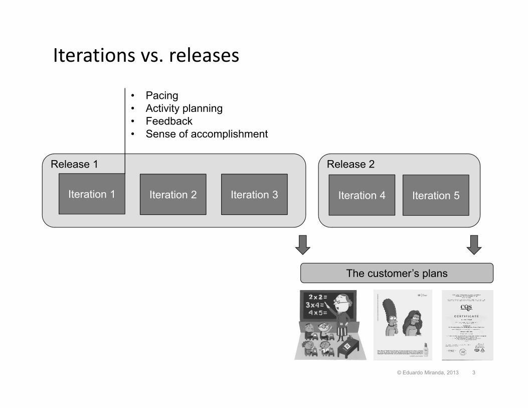
Release 1 Release 2

Iterations vs. releases

Iteration 1 Iteration 2 Iteration 3 Iteration 4

The customer’s plans

Iteration 5


• Pacing• Activity planning• Feedback• Sense of accomplishment

The release planning problem

• Release planning is the process of deciding when and with what features a working version of a software product will be made available to its customers

• The process must take into consideration business objectives, technical and functional dependencies and resource constrains


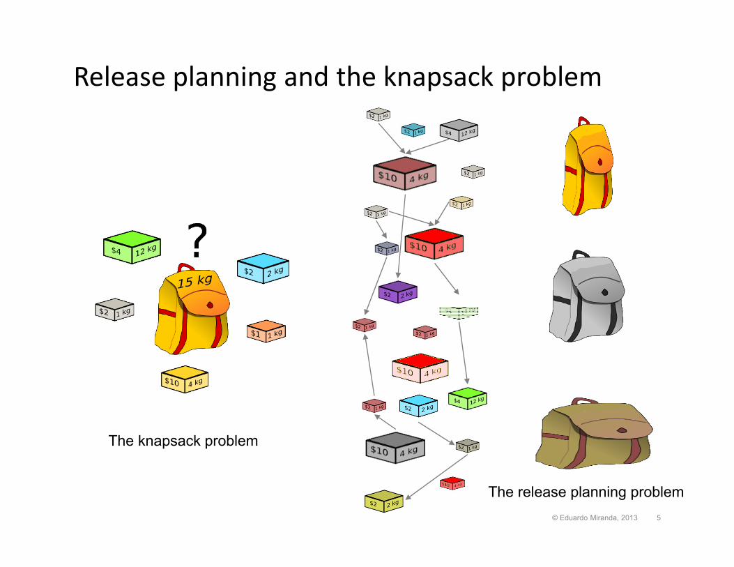
Release planning and the knapsack problem

The knapsack problem

The release planning problem© Eduardo Miranda, 2013 5

Release planning methods (1)

• Must Have, Should Have, Could Have, Won’t have (MoSCoW) Method; D. Clegg 1994 & DSDM Consortium– Unstated customer preference & delivery certainty– Assumes three releases within a predefined time box– Manual method, qualitative

• Statistically Planned Incremental Delivery (SPID); E. Miranda, 2002– Unstated customer preference & delivery certainty– Assumes a defined number of releases within a predefined time box– Manual. Uses subjective probabilities and statistical concepts to guarantee

the delivery of the most important features consistent with the basic assessments

• Evolve, D. Greer & G. Ruhe, 2003– Maximizes an objective function defined in terms of benefits & penalties– Inputs: Features’ value, criticality and required effort; stakeholders weight,

effort constraints for release– Undefined number of releases. Genetic algorithm makes recommendation

of k best solutions for the immediate release, customer choose and iterates


Release planning methods (2)

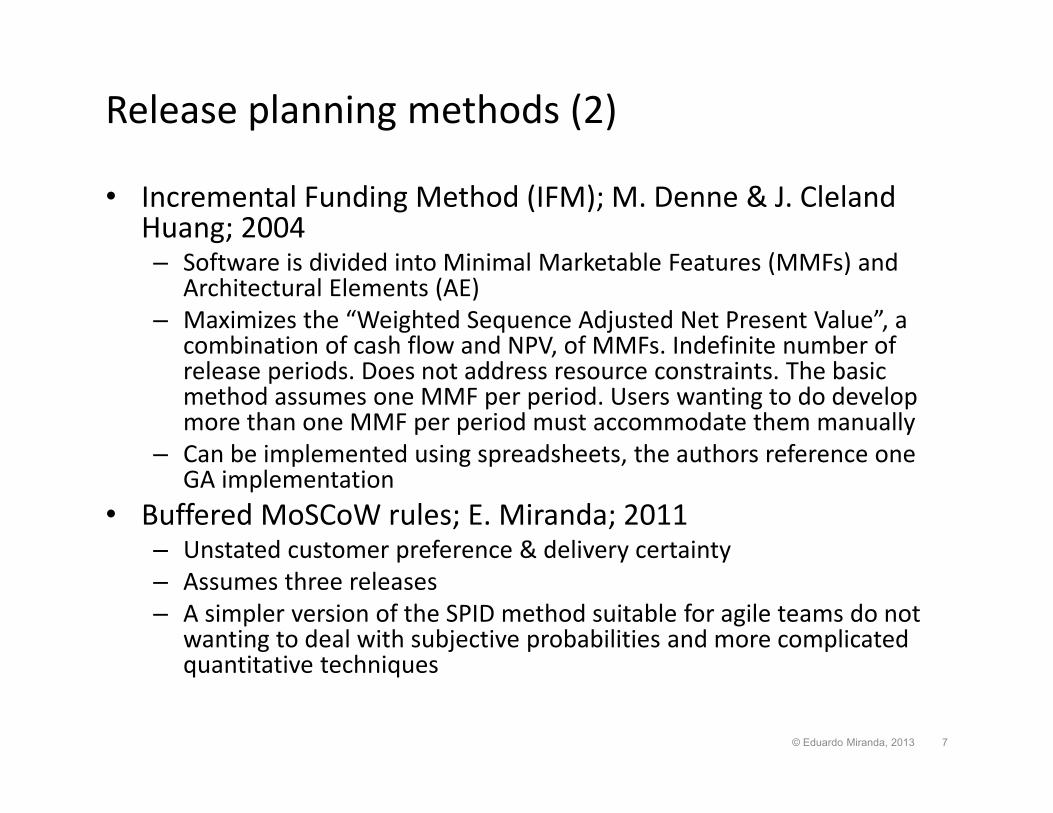
• Incremental Funding Method (IFM); M. Denne & J. Cleland Huang; 2004– Software is divided into Minimal Marketable Features (MMFs) and

Architectural Elements (AE)– Maximizes the “Weighted Sequence Adjusted Net Present Value”, a

combination of cash flow and NPV, of MMFs. Indefinite number of release periods. Does not address resource constraints. The basic method assumes one MMF per period. Users wanting to do develop more than one MMF per period must accommodate them manually

– Can be implemented using spreadsheets, the authors reference one GA implementation

• Buffered MoSCoW rules; E. Miranda; 2011– Unstated customer preference & delivery certainty– Assumes three releases– A simpler version of the SPID method suitable for agile teams do not

wanting to deal with subjective probabilities and more complicated quantitative techniques


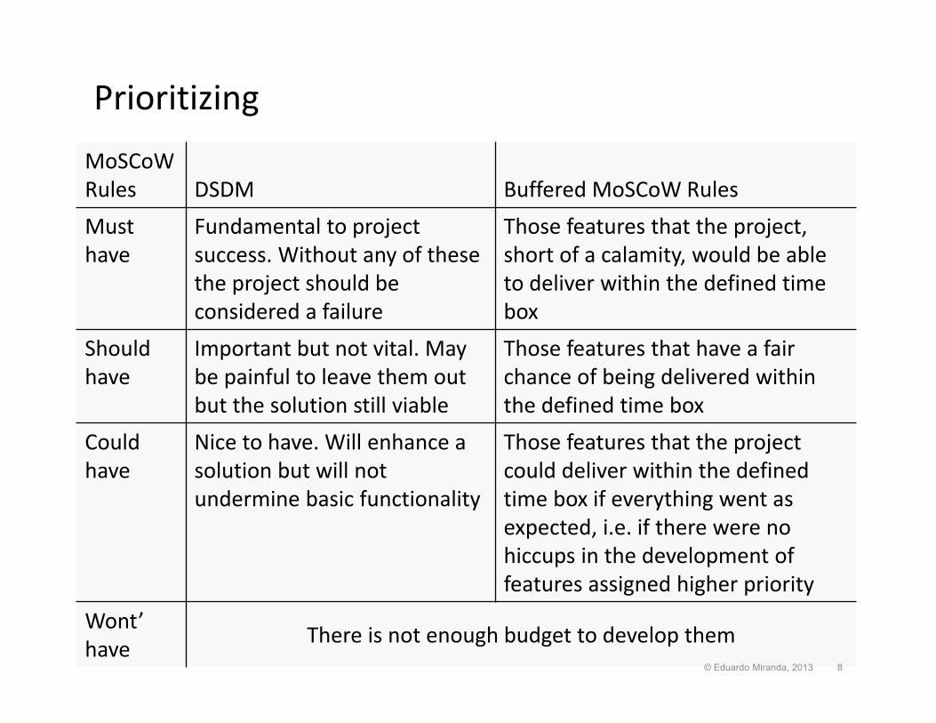
Prioritizing MoSCoWRules DSDM Buffered MoSCoW RulesMust have

Fundamental to project success. Without any of thesethe project should be considered a failure

Those features that the project, short of a calamity, would be able to deliver within the defined time box

Should have

Important but not vital. May be painful to leave them out but the solution still viable

Those features that have a fair chance of being delivered within the defined time box

Couldhave

Nice to have. Will enhance a solution but will not undermine basic functionality

Those features that the project could deliver within the defined time box if everything went as expected, i.e. if there were no hiccups in the development of features assigned higher priority

Wont’ have There is not enough budget to develop them


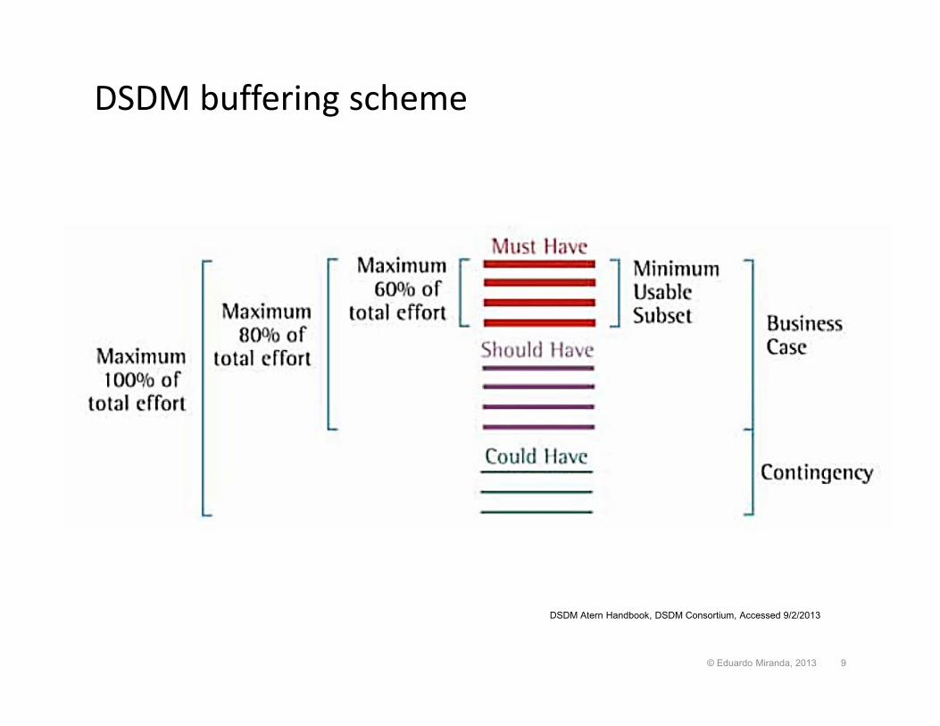
DSDM buffering scheme

DSDM Atern Handbook, DSDM Consortium, Accessed 9/2/2013


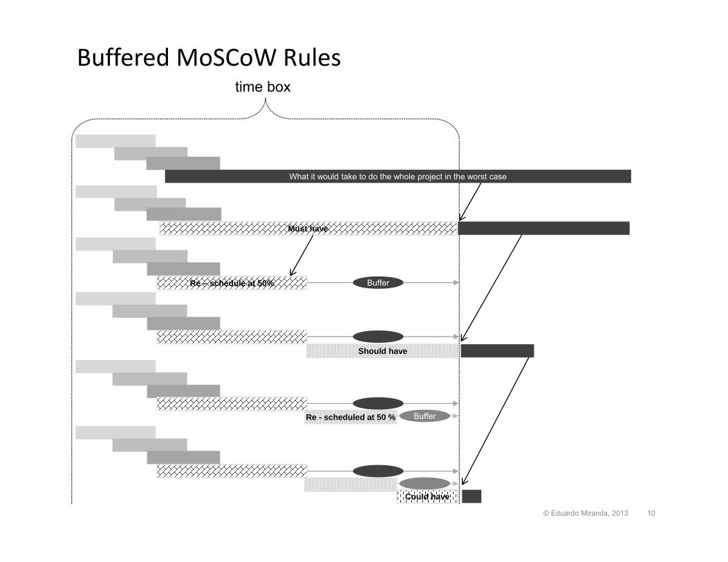
Buffered MoSCoW Rulestime box

What it would take to do the whole project in the worst case

Must have

Re – schedule at 50% Buffer

Should have

BufferRe - scheduled at 50 %

Could have


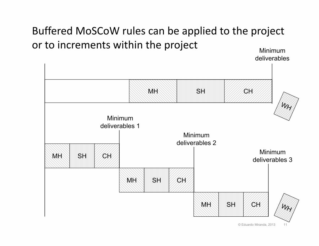
Buffered MoSCoW rules can be applied to the project or to increments within the project

Minimum deliverables

Minimum deliverables 1




MH SH CH

MH SH CH

MH SH CH

MH SH CH

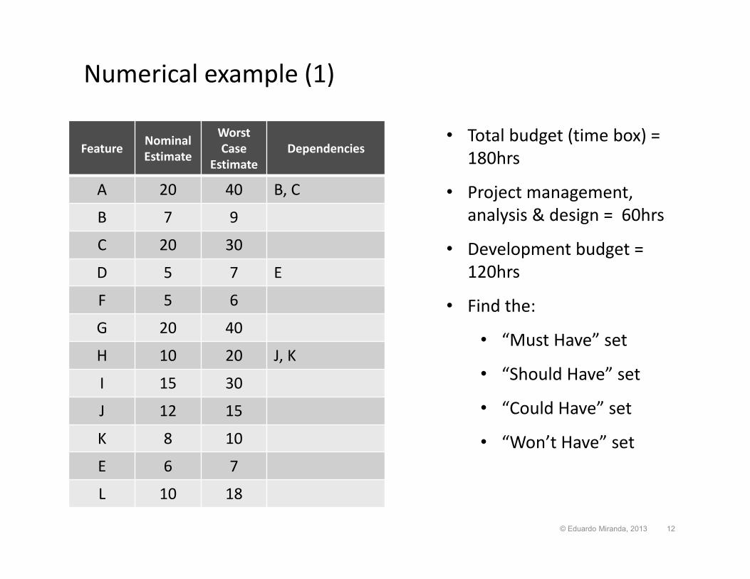
Numerical example (1)

Features 50%Estimate

90%Estimate Dependencies

A 20 40 B, C

B 7 9

C 20 30

D 5 7 E

E 5 6

F 20 40

G 10 20

H 15 30 J, K

I 12 15

J 8 10

K 6 7

L 10 18

• Total budget (time box) = 180hrs

• Project management, analysis & design = 60hrs

• Development budget = 120hrs

• Find the:

• “Must Have” set

• “Should Have” set

• “Could Have” set

• “Won’t Have” set

Feature Nominal Estimate

Worst Case

EstimateDependencies

A 20 40 B, C

B 7 9

C 20 30

D 5 7 E

F 5 6

G 20 40

H 10 20 J, K

I 15 30

J 12 15

K 8 10

E 6 7

L 10 18


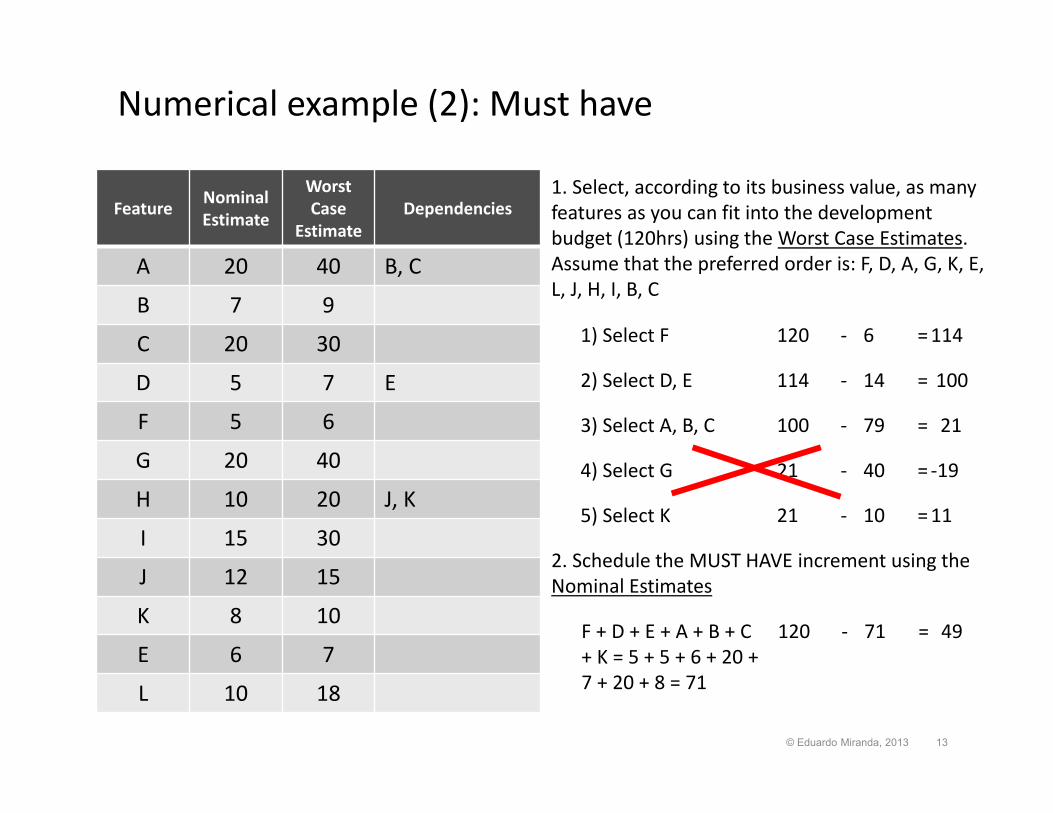
Numerical example (2): Must have


Worst Case


A 20 40 B, C

B 7 9

C 20 30

D 5 7 E

F 5 6

G 20 40

H 10 20 J, K

I 15 30

J 12 15

K 8 10

E 6 7

L 10 18

3) Select A, B, C 79 21100 ‐ =

2) Select D, E 14 100114 ‐ =

4) Select G 40 ‐1921 ‐ =

1) Select F 6 114120 ‐ =

5) Select K 10 1121 ‐ =

1. Select, according to its business value, as many features as you can fit into the development budget (120hrs) using the Worst Case Estimates. Assume that the preferred order is: F, D, A, G, K, E, L, J, H, I, B, C

2. Schedule the MUST HAVE increment using the Nominal Estimates

F + D + E + A + B + C + K = 5 + 5 + 6 + 20 + 7 + 20 + 8 = 71

71 49120 ‐ =


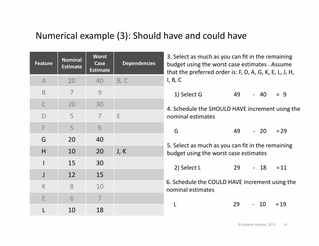
Numerical example (3): Should have and could have


Worst Case


A 20 40 B, C

B 7 9

C 20 30

D 5 7 E

F 5 6

G 20 40

H 10 20 J, K

I 15 30

J 12 15

K 8 10

E 6 7

L 10 18

1) Select G 40 949 ‐ =

G 20 2949 ‐ =

2) Select L 18 1129 ‐ =

3. Select as much as you can fit in the remaining budget using the worst case estimates . Assume that the preferred order is: F, D, A, G, K, E, L, J, H, I, B, C

4. Schedule the SHOULD HAVE increment using the nominal estimates

5. Select as much as you can fit in the remaining budget using the worst case estimates

6. Schedule the COULD HAVE increment using the nominal estimates

L 10 1929 ‐ =


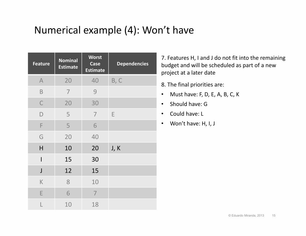
Numerical example (4): Won’t have


Worst Case


A 20 40 B, C

B 7 9

C 20 30

D 5 7 E

F 5 6

G 20 40

H 10 20 J, K

I 15 30

J 12 15

K 8 10

E 6 7

L 10 18

7. Features H, I and J do not fit into the remaining budget and will be scheduled as part of a new project at a later date

8. The final priorities are:

• Must have: F, D, E, A, B, C, K

• Should have: G

• Could have: L

• Won’t have: H, I, J


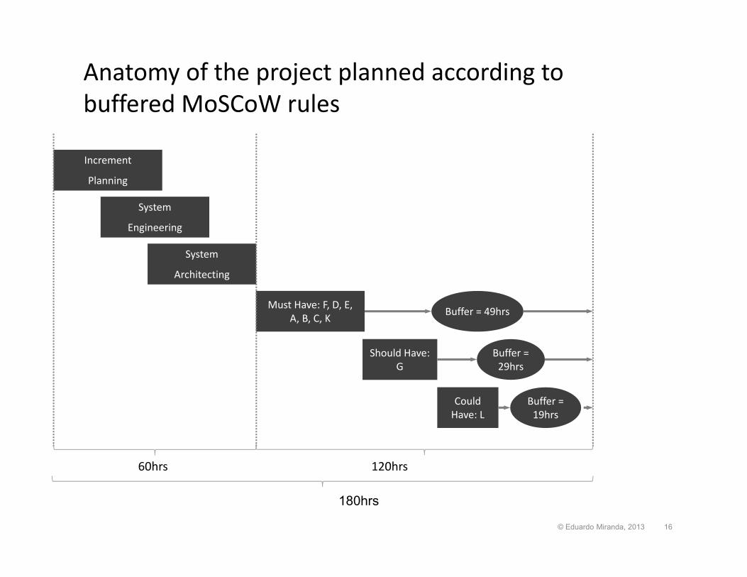
Anatomy of the project planned according to buffered MoSCoW rules

Increment

Planning

System

Engineering

System

Architecting

Must Have: F, D, E, A, B, C, K

Should Have: G

Could Have: L

Buffer = 49hrs

Buffer = 29hrs

60hrs 120hrs

180hrs

Buffer = 19hrs


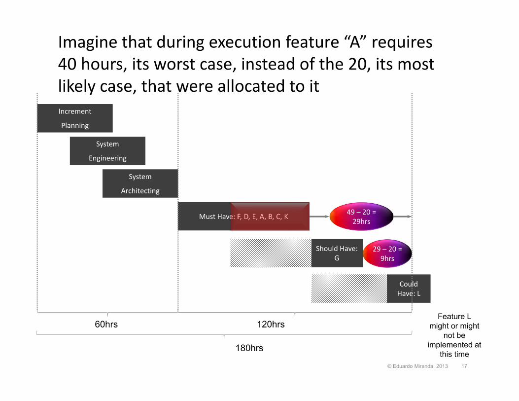
29 – 20 = 9hrs

49 – 20 = 29hrs

Imagine that during execution feature “A” requires 40 hours, its worst case, instead of the 20, its most likely case, that were allocated to itIncrement

Planning

System

Engineering

System

Architecting

Must Have: F, D, E, A, B, C, K

Should Have: G

Could Have: L

60hrs 120hrs

180hrs

Feature L might or might

not be implemented at

this time© Eduardo Miranda, 2013 17

FAQ

• What it is the extent of the guarantee?• How do you handle infrastructure work, changes and defects?

• Contracts & Employee incentives– Why will developers do something more than the “must have”?

– Why will a client accept less than “everything”?

• What do you loose by using the worst case scenarios to simplify the problem?


What it is the extent of the guarantee?

• Results at the project level are consistent with assertions made at the lower levels

• If the assertions are wrong, the results will be consistently wrong


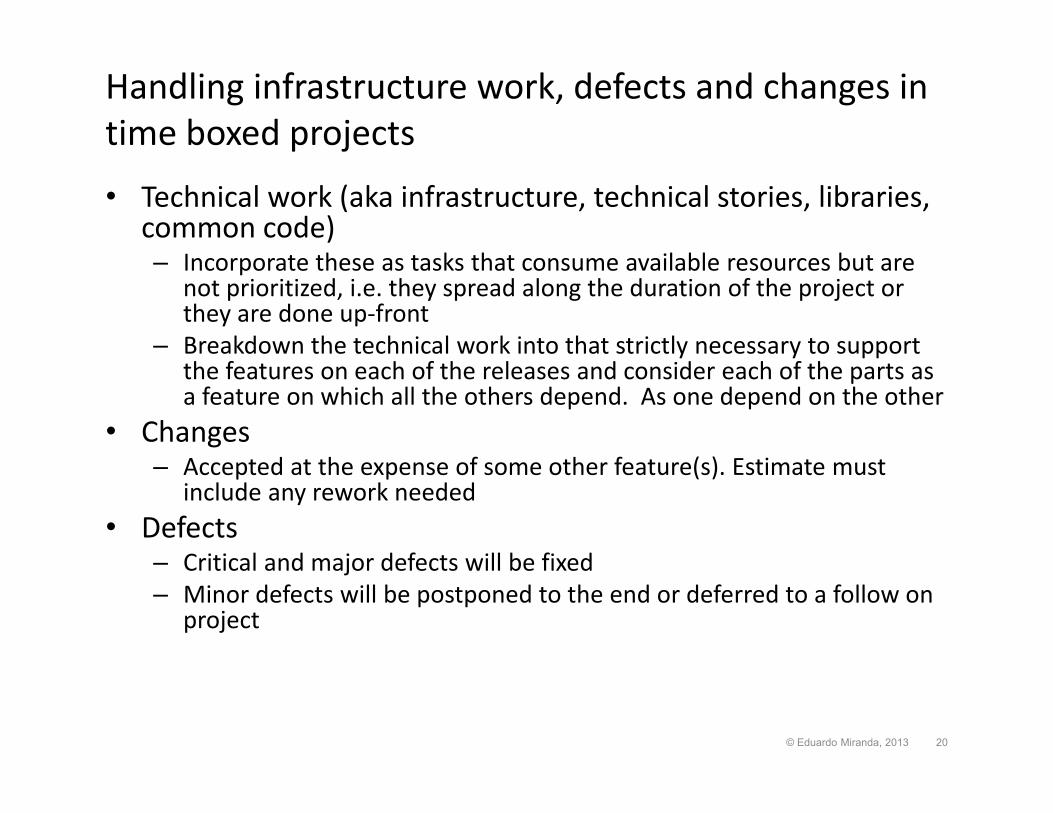
Handling infrastructure work, defects and changes in time boxed projects

• Technical work (aka infrastructure, technical stories, libraries, common code)– Incorporate these as tasks that consume available resources but are

not prioritized, i.e. they spread along the duration of the project or they are done up‐front

– Breakdown the technical work into that strictly necessary to support the features on each of the releases and consider each of the parts as a feature on which all the others depend. As one depend on the other

• Changes– Accepted at the expense of some other feature(s). Estimate must

include any rework needed• Defects

– Critical and major defects will be fixed– Minor defects will be postponed to the end or deferred to a follow on

project


Incentives & contracts

• Associate employee rewards with release completion, suppress overtime and provide larger bonuses after successful deployment

• Contracts must include price incentives/penalties contingent on deliveries

• Supplier must take in consideration the probabilities of successful deliveries to price the contract


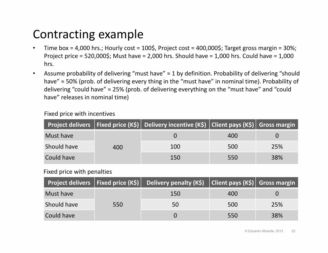
Contracting example• Time box = 4,000 hrs.; Hourly cost = 100$, Project cost = 400,000$; Target gross margin = 30%;

Project price = 520,000$; Must have = 2,000 hrs. Should have = 1,000 hrs. Could have = 1,000 hrs.

• Assume probability of delivering “must have” ≈ 1 by definition. Probability of delivering “should have” ≈ 50% (prob. of delivering every thing in the “must have” in nominal time). Probability of delivering “could have” ≈ 25% (prob. of delivering everything on the “must have” and “could have” releases in nominal time)


Project delivers Fixed price (K$) Delivery incentive (K$) Client pays (K$) Gross margin

Must have

400

0 400 0

Should have 100 500 25%

Could have 150 550 38%

Fixed price with incentives

Project delivers Fixed price (K$) Delivery penalty (K$) Client pays (K$) Gross margin

Must have

550

150 400 0

Should have 50 500 25%

Could have 0 550 38%

Fixed price with penalties

Employee incentives


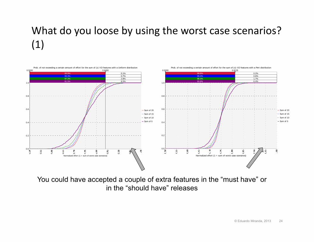
What do you loose by using the worst case scenarios? (1)

99.8% 0.2%99.4% 0.6%98.3% 1.7%93.6% 6.4%

0.5000 0.8125

Normalized effort (1 = sum of worst case scenarios)

0.0

0.2

0.4

0.6

0.8

1.0

Prob. of not exceeding a certain amount of effort for the sum of (x) IID features with a Pert distribution

Sum of 20

Sum of 15

Sum of 10

Sum of 5

99.9% 0.1%99.3% 0.7%97.2% 2.8%91.5% 8.5%

0.5000 0.8400


0.0

0.2

0.4

0.6

0.8

1.0

Prob. of not exceeding a certain amount of effort for the sum of (x) IID features with a Uniform distribution

Sum of 20

Sum of 15

Sum of 10

Sum of 5

You could have accepted a couple of extra features in the “must have” or in the “should have” releases


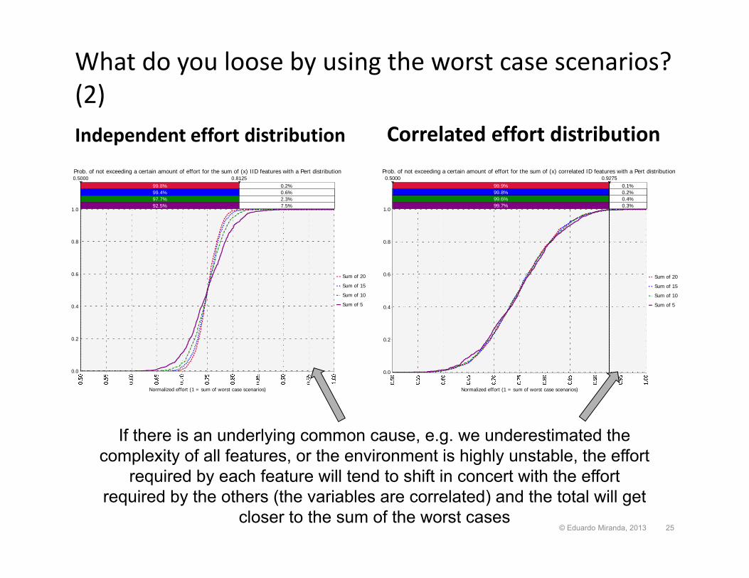
What do you loose by using the worst case scenarios? (2)Independent effort distribution

99.8% 0.2%99.4% 0.6%97.7% 2.3%92.5% 7.5%

0.5000 0.8125


0.0

0.2

0.4

0.6

0.8

1.0

Prob. of not exceeding a certain amount of effort for the sum of (x) IID features with a Pert distribution

Sum of 20

Sum of 15

Sum of 10

Sum of 5

Correlated effort distribution

99.9% 0.1%99.8% 0.2%99.6% 0.4%99.7% 0.3%

0.5000 0.9275


0.0

0.2

0.4

0.6

0.8

1.0

Prob. of not exceeding a certain amount of effort for the sum of (x) correlated ID features with a Pert distribution

Sum of 20

Sum of 15

Sum of 10

Sum of 5


If there is an underlying common cause, e.g. we underestimated the complexity of all features, or the environment is highly unstable, the effort

required by each feature will tend to shift in concert with the effort required by the others (the variables are correlated) and the total will get

closer to the sum of the worst cases

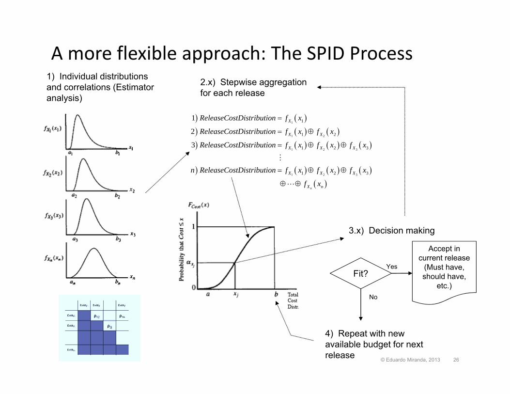
A more flexible approach: The SPID Process

1

1 2

1 2 3

1 2 3

1

1 2

1 2 3

1 2 3

1

2

3

n

X

X X

X X X

X X X

X n

ReleaseCostDistribution f x

ReleaseCostDistribution f x f x

ReleaseCostDistribution f x f x f x

n ReleaseCostDistribution f x f x f x

f x

Fit?

1) Individual distributions and correlations (Estimator analysis)

2.x) Stepwise aggregation for each release

Accept in current release

(Must have, should have,

etc.)

3.x) Decision making

Yes

4) Repeat with new available budget for next release

No


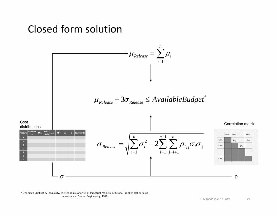
Closed form solution

ρσ

E. Miranda © 2011, CMU 27

Correlation matrixCost distributions

1

n

Release ii

12

, j1 1 1

2n n n

Release i i j ii i j i

* One sided Chebyshev inequality, The Economic Analysis of Industrial Projects, L. Bussey, Prentice‐Hall series in Industrial and System Engineering, 1978

*3Release Release AvailableBudget

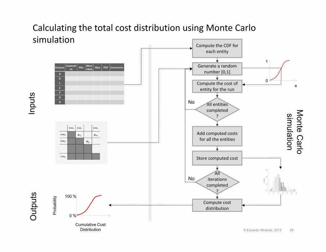
Calculating the total cost distribution using Monte Carlo simulation

Monte C

arlo sim

ulationCompute the CDF for

each entity

Generate a random number [0,1]

Compute the cost of entity for the run

All entities completed

?

0

1

e

Add computed costs for all the entities

All iterations completed

?

Compute cost distribution

Store computed cost

No

No

0 %

100 %

Cumulative Cost Distribution

Pro

babi

lity

Inpu

tsO

utpu

ts


Summary• We have presented a simple prioritization procedure that can be applied

to the ranking of requirements at the release as well as the project level. The procedure does not only captures customer preferences, but by constraining the number of features in the “must have” set as a function of the uncertainty of the underlying estimates, is able to offer project sponsors a high degree of reassurance in regards to the delivered of an agreed level of software functionality by the end of the time box

• To be workable for the supplier and the employer, the contract between the parts must incorporate the notion that an agreed partial delivery is an acceptable, although not preferred, outcome

• Similarly, employees must be engaged into the process to prevent free rides

• The method simplicity is not free. It comes at the expense of the claims we can make about the likelihood of delivering a given functionality and a conservative buffer. Users seeking to make more definitive probabilistic statements or optimize the buffer size should consider the use of a more sophisticated approach such as SPID (described in Planning and Executing Time Bound Projects, E. Miranda, 2002)


Questions?


release planning & buffered moscow rules

Documents

technicala eduardo miranda

dsdm consortium

denne j