release 1.0.1 k.a. kvåle
TRANSCRIPT

KOMARelease 1.0.1
K.A. Kvåle
Jan 20, 2022


CONTENTS:
1 Installation and usage 31.1 Python . . . . . . . . . . . . . . . . . . . . . . . . . . . . . . . . . . . . . . . . . . . . . . . . . . 31.2 MATLAB . . . . . . . . . . . . . . . . . . . . . . . . . . . . . . . . . . . . . . . . . . . . . . . . . 3
2 Python code reference 5
3 MATLAB code reference 73.1 Operational modal analysis module . . . . . . . . . . . . . . . . . . . . . . . . . . . . . . . . . . . 73.2 Modal post-processing module . . . . . . . . . . . . . . . . . . . . . . . . . . . . . . . . . . . . . . 83.3 Visualization module . . . . . . . . . . . . . . . . . . . . . . . . . . . . . . . . . . . . . . . . . . . 10
4 Examples 154.1 Python example: shear frame . . . . . . . . . . . . . . . . . . . . . . . . . . . . . . . . . . . . . . 154.2 MATLAB example: shear frame . . . . . . . . . . . . . . . . . . . . . . . . . . . . . . . . . . . . . 194.3 MATLAB exaple: visualization of beam modes . . . . . . . . . . . . . . . . . . . . . . . . . . . . . 24
5 Licensing information 27
6 References 29
7 Acknowledgements 31
8 Indices and tables 33
Bibliography 35
MATLAB Module Index 37
Index 39
i

ii

KOMA, Release 1.0.1
KOMA is a package for operational modal analysis, with core functionality available both in Python and MATLABlanguages. For additional details about the implementation of the covariance-driven stochastic subspace identificationalgorithm please refer to [5]. Data-SSI and FDD are implemented in the MATLAB version of KOMA. For automaticOMA and clustering analysis, please refer to [6]. More information and functionality will be added after publicationof the cited paper.
CONTENTS: 1

KOMA, Release 1.0.1
2 CONTENTS:

CHAPTER
ONE
INSTALLATION AND USAGE
1.1 Python
Either download the repository to your computer and install, e.g. by pip
pip install .
or install directly from the python package index.
pip install git+https://www.github.com/knutankv/koma.git@master
Thereafter, import the package modules, exemplified for the `oma´ module, as follows:
import koma.oma
1.2 MATLAB
Download or clone repository. Folder containing package root has to be in the MATLAB path:
addpath('C:/Users/knutankv/git-repos/koma/');
Ideally this is done permanently, such that it is always accessible. Then, the package can be imported with thefollowing command:
import koma.*
Now all the subroutines of the package are accessible through
koma.function_name
E.g., to use the function covssi.m located at . . . /+koma/+oma/ the following syntax is applied:
[lambda,phi,order] = koma.oma.covssi(data, fs, i, 'order', order);
Functions inside private folders are accessible only from functions inside the folder at the root of the private folder.
3

KOMA, Release 1.0.1
4 Chapter 1. Installation and usage

CHAPTER
TWO
PYTHON CODE REFERENCE
5

KOMA, Release 1.0.1
6 Chapter 2. Python code reference

CHAPTER
THREE
MATLAB CODE REFERENCE
3.1 Operational modal analysis module
koma.oma.covssi(data, fs, blockrows, varargin)Covariance-driven SSI.
Parameters
• data (double) – data matrix, with channels stacked column-wise (n_samples-by-n_channels)
• fs (double) – sampling frequency
• blockrows (int) – maximum number of block rows
• orders ([], optional) – array or list of what orders to include
• weighting ('none', optional) – what weighting type to use (‘none’ or ‘br’, or‘cva’)
• matrix_type ('matrix_type', optional) – what matrix type formulation tobase computation on (‘hankel’ or ‘toeplitz’)
• algorithm ('shift', optional) – what algorithm to use (‘shift’ or ‘standard’ -when using ‘standard’ the method is equivalent to NExt-ERA)
• showinfo (True, optional) – whether or not to print information during computa-tion
• balance (True, optional) – whether or not to conduct balancing to the cross-correlation matrices prior to matrix operations (Cholesky and SVD)
Returns
• lambd (double) – cell array with vectors for all modes corresponding to all orders
• phi (double) – cell array with matrices containing all mode shapes corresponding to allorders
• order (int) – vector with all orders
• weighting (str) – the applied weighting algorithm (not always equal input)
7

KOMA, Release 1.0.1
References
• Hermans and van Der Auweraer [1] (1 in code)
• Van Overschee and de Moor [2] (2 in code)
• Rainieri and Fabbrocino [3] (3 in code)
• Pridham and Wilson [4] (4 in code)
koma.oma.ddssi(data, fs, blockrows, varargin)Data-driven SSI.
Parameters
• data (double) – data matrix, with channels stacked column-wise (n_samples-by-n_channels)
• fs (double) – sampling frequency
• blockrows (int) – maximum number of block rows
• orders ([], optional) – array or list of what orders to include
• weighting ('upc', optional) – what weighting type to use (‘pc’, ‘upc’, ‘cva’)
• algorithm (2, optional) – what algorithm to use with reference to Van Overscheeand de Moor [2] (1, 2 [fastest], or 3)
• showinfo (true, optional) – whether or not to print information during computa-tion
Returns
• lambda (double) – cell array with vectors for all modes corresponding to all orders
• phi (double) – cell array with matrices containing all mode shapes corresponding to allorders
• orders (int) – vector with all orders
• weighting (str) – the applied weighting algorithm (not always equal input)
References
• Van Overschee and de Moor [2] (1 in code)
• Rainieri and Fabbrocino [3] (2 in code)
3.2 Modal post-processing module
koma.modal.find_stable_poles(lambda, phi, order, s, stabcrit, indicator)Post-processing of Cov-SSI results, to establish modes (stable poles) from all poles.
Parameters
• lambda (double) – cell array of arrays with complex-valued eigenvalues, one cell entryper order
• phi (double) – cell array of matrices with complex-valued eigevectors (stacked column-wise), one cell entry per order
8 Chapter 3. MATLAB code reference

KOMA, Release 1.0.1
• orders (int) – 1d array with orders corresponding to the cell array entries in lambd andphi
• s (int) – stability level, see [5]
• stabcrit ({'freq': 0.05, 'damping':0.1, 'mac': 0.1}, optional)– criteria to be fulfilled for pole to be deemed stable
• indicator ('freq', optional) – what modal indicator to use (‘freq’ or ‘mac’)
Returns
• lambd_stab (double) – array with complex-valued eigenvalues deemed stable
• phi_stab (double) – 2d array with complex-valued eigenvectors (stacked as columns), eachcolumn corresponds to a mode
• order_stab (int) – corresponding order for each stable mode
• idx_stab (int) – indices of poles (within its order from the input) given in lambd_stabdeemed stable (for indexing post)
References
Kvaale et al. [5]
koma.modal.pick_stable_modes(lambda_stab, phi_stab, slack, varargin)Pick stable modes from arrays of lambdas. Use like this: [lambda,phi,order,idx] = pick_stable_modes(lambda,phi, slack, phi_ref)
Parameters
• lambd_stab (double) – array with complex-valued eigenvalues deemed stable byfind_stable_poles
• phi_stab (double) – 2d array with complex-valued eigenvectors (stacked as columns)deemed stable by find_stable_poles, each column corresponds to a mode
• slack (double) – allowed relative deviance between different modes input for them tobe clustered together as the same mode (3-by-1, [freq, xi, mac])
• phi_ref (double, optional) – reference modal matrix, MAC slack value corre-sponds to slack from this if input. If not wanted, use []. Note slack(1) and slack(2) notused in this mode!
• maxmacdeviance (0.2, optional) – restricts the deviance from the ref. mode shape(value of 0.2 => MAC>0.8)
• onlyone (true, optional) – if true, only one mode is identified per reference - oth-erwise, multiple modes within slack limits are selected
• mean (true, optional) – if true, the statistical mean of all within slack is used insteadof the single pole with largest MAC. The standard deviations are reported in lambda_std andphi_std. Only applicable when phi_ref is input.
• slack_mode ('all', optional) – ‘all’ (all have to be within) or ‘one’ (okay if onlyone is)
Returns
• lambda_picked (double) – array with selected lambdas
• phi_picked (double) – phi with stable mode shapes (stacked column-wise)
3.2. Modal post-processing module 9
KOMA, Release 1.0.1
• statistics (struct) – structure with statistics for each mode cluster
koma.modal.resasref(lambda, phi, phi_ref, maccrit)Restructure modes as reference (shuffle the mode numbering).
Parameters
• lambd (double) – array of all eigenvalues
• phi (double) – modal transformtaion matrix (all mode shapes), stacked column-wise
• phi_ref (int) – modal transformation matrix from reference (the one to sort after)
• maccrit (int) – MAC criterion (nan/empty if not satisfied)
Returns
• lambda_save (double) – output lambda (picked and sorted from lambda)
• phi_save (double) – output phi (picked and sorted from phi)
• okrefidx (int) – indices related to reference that are deemed ok
• okididx (int) – indices related to input phi that are deemed ok
koma.modal.xmacmat(phi1, varargin)Modal assurance criterion numbers, cross-matrix between two modal transformation matrices (modes stackedas columns).
Parameters
• phi1 (double) – reference modes
• phi2 (double, optional) – modes to compare with, if not given (i.e., equal defaultvalue None), phi1 vs phi1 is assumed
• conjugates (true, optional) – check the complex conjugates of all modes as well(should normally be true)
Returns macs – matrix of MAC numbers
Return type boolean
3.3 Visualization module
koma.vis.animate_mode(phi, w, griddef, elements, slave, active_nodes, varargin)Plot translational part of mode, by inputting translational mode shape.
Parameters
• phi (double) – complex-valued mode shape to plot (translational part only)
• w (double) – scalar frequency value (rad/s) in which to animate the mode vibration
• griddef (double) – matrix defining the nodes of the model (see Notes for details)
• elements (int) – matrix defining the elements of the model, connecting the node num-bers together as patches or beams (see Notes for details)
• slave (int) – matrix defining linear relations between DOFs (see Notes for details)
• active_nodes (int) – Index of nodes that are active (highlighted). If empty, all nodesare assumed active!
10 Chapter 3. MATLAB code reference

KOMA, Release 1.0.1
• movietitle (str, optional) – title (name) for movie file (if not given a dialog willappear)
• fps (30, optional) – frames per second of generated video file
• laps (1, optional) – laps to animate the mode
• rotations (0, optional) – rotations (pan-style) about the z-axis during animation
• xi (0, optional) – damping estimate for mode, used for animation
• cam (0, optional) – as for plot_mode, camera defintions
• complexmode (true, optional) – wheter or not to plot the complex mode
Notes
All of the optional inputs to plot_mode are valid as input as well. Please refer to doc of plot_mode.
koma.vis.plot_mode(phi, griddef, elements, slave, active_nodes, varargin)Plot translational part of mode, by inputting translational mode shape.
Parameters
• phi (double) – complex-valued mode shape to plot (translational part only)
• griddef (double) – matrix defining the nodes of the model (see Notes for details)
• elements (int) – matrix defining the elements of the model, connecting the node num-bers together as patches or beams (see Notes for details)
• slave (int) – matrix defining linear relations between DOFs (see Notes for details)
• active_nodes (int) – Index of nodes that are active (highlighted). If empty, all nodesare assumed active!
• scaling ([], optional) – numerical value defining linear scaling of displacementvector ([] results in automatic scaling).
• scalefactor (1, optional) – second factor used to adjust automatic scaling
• axishandle ([], optional) – axis handle to make plot in
• cam ([], optional) – camera properties
• cmdir ('abs', optional) – component to base the colormap on (‘abs’, ‘x’, ‘y’ or ‘z’)
• colormap ([], optional) – predefined colormap vector (max and min val.), [] leadsto auto.
• plots ('both', optional) – which deformation state to plot (‘both, ‘undeformed’,or ‘deformed’)
• labels ('none', optional) – put labels on the figure (which state)? (‘both’, ‘unde-formed’, ‘deformed’, or ‘none’)
• title ('', optional) – title of figure, at position as defined in cam
• axis (false, optional) – whether or not to show axis
• edge ('both', optional) – show edge color for surfaces (‘both’, ‘undeformed’, ‘de-formed’, ‘none’)
• nodes ('both', optional) – switch for nodes (‘both’,’active’, or’inactive’)
• lines (true, optional) – switch for lines showing displacements
3.3. Visualization module 11

KOMA, Release 1.0.1
• renderer ('zbuffer', optional) – figure renderer (‘zbuffer’, ‘painters’, or‘opengl’)
• maxreal (true, optional) – make the real part as big as possible or not
• linewidth (1, optional) – line width on edges and lines
Returns
• axis_handle (obj) – handle of axis object
• scaling (double) – used scaling
• cm (obj) – used colormap
Notes
griddef, elements and slave follow the exact same definition as for the MACEC toolbox. See details below.
griddef is exemplified as follows for arbitrary three nodes (exclude header):
Node no. X Y Z1 0 0 12 0.1 0.2 0.33 -2 0.3 10
3D input is required even if the analysis is 2D. Other than that, its definition is assumed self-explanatory.
elements is exemplified as follows (exclude header):
Node 1 Node 2 Node 31 2 32 3 0
This example creates two elements: (1) a patch between nodes 1,2, and 3 and (2) a beam element betweennodes 2 and 3 (node 3 = 0 => beam element). If no patch elements are needed, the table’s first two columns aresufficient.
slave is exemplified as follows (exclude header):
Master X Y Z Slave X Y Z1 1 0 0 2 0.3 0.7 01 0 1 0 4 0 1 03 1 0 0 5 1 0 0
The displacement of the slave node is defined based on the displacement of the master node in either X, Y orZ direction. A unity value indicates that this is the local DOF to use as master (keep the others equal 0). Theamplitudes of the different DOFs of the slave nodes are defined by the values in the latter three columns.
• The example table above describes the following slave-master definition:
– Node 1, DOF X, dictates the motion of node 2 by a factor 0.3 on the X-component and a factor of 0.7on the Y-component.
– Node 1, DOF Y, dictates the motion of node 4 by a factor of 1 on the Y-component.
12 Chapter 3. MATLAB code reference

KOMA, Release 1.0.1
– Node 3, DOF X, dictates the motion of node 5 by a factor of 1 on the X-component.
koma.vis.stabplot(lambda, phi, orders, varargin)Plot stabilization plot from lambda and phi arrays (output from covssi).
Parameters
• lambda (double) – cell array of arrays with complex-valued eigenvalues, one cell entryper order
• phi (double) – cell array of matrices with complex-valued eigevectors (stacked column-wise), one cell entry per order matrix)
• orders (int) – 1d array with orders corresponding to the cell array entries in lambd andphi
• s (int, optional) – stability level, see [5]
• stabcrit ({'freq': 0.05, 'damping':0.1, 'mac': 0.1}, optional)– criteria to be fulfilled for pole to be deemed stable
• indicator ('freq', optional) – what modal indicator to use (‘freq’ or ‘mac’)
• plots ('both', optional) – what poles to plot (‘both’ or ‘stable’)
• markers ('.', optional) – first value applies to all poles, second to stable poles
• markersize ([36], optional) – first value applies to all poles, second to stablepoles
• colors ({'r' 'k'}, optional) – first value applies to all poles, second to stablepoles
• picked_lambda ([], optional) – plot vertical lines of these lambda values
• picked_error ([], optional) – plot corresponding error bar (frequency,abs(lambda), and not lambda) relying on thirdparty contribution by Jos van der Geest, her-rorbar
• figure ([], optional) – specified figure handle
• selection (false, optional) – whether or not to enable selection of poles for plot-ting and output
• grid ([], optional) – if selection is true, this is used to plot mode shape
• elements ([], optional) – if selection is true, this is used to plot mode shape
• slave ([], optional) – if selection is true, this is used to plot mode shape
• active_nodes ([], optional) – if selection is true, this is used to plot mode shape
References
Jos (10584) (2020). HERRORBAR (https://www.mathworks.com/matlabcentral/fileexchange/3963-herrorbar),MATLAB Central File Exchange. Retrieved April 21, 2020.
3.3. Visualization module 13

KOMA, Release 1.0.1
14 Chapter 3. MATLAB code reference

CHAPTER
FOUR
EXAMPLES
Some simple examples are provided for both Python and MATLAB. More will be added at a later point in time.
4.1 Python example: shear frame
[1]: import koma.oma, koma.plot
import numpy as npimport matplotlib.pyplot as plt
from scipy.signal import detrend, welch
import pandas as pd
4.1.1 System definition
[2]: K = np.array([[8000, -8000,0], [-8000, 16000, -8000], [0, -8000, 16000]])C = np.array([[10, 0,0], [0, 10, 0], [0, 0, 10]])M = np.array([[500,0,0], [0, 500,0], [0, 0, 500]])
4.1.2 Analytical eigenvalue solution
[3]: from knutils.modal import statespace as to_A
A = to_A(K, C, M) # establish state matrix based on K, C and Mlambdai, qi = np.linalg.eig(A)
ix = np.argsort(np.abs(lambdai))xi = -np.real(lambdai)/np.abs(lambdai)
print(xi[ix[::2]]*100)
[0.5617449 0.20048443 0.13873953]
15

KOMA, Release 1.0.1
4.1.3 Load data and define input
[38]: # Import and specify properties of input datadf = pd.read_csv('shear_frame_simulation.csv', sep=',',header=None)data = df.values # data including noisefs = 3.0t = np.arange(0,1/fs*(data.shape[0]),1/fs)
# Cov-SSI settingsi = 20s = 4orders = np.arange(2, 50+2, 2)stabcrit = {'freq':0.2, 'damping': 0.2, 'mac': 0.3}
# Noise specificationnoise_factor = 1.0
4.1.4 Add artificial noise and plot response
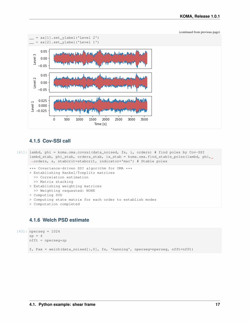
[40]: noise = np.std(data) * noise_factordata_noised = data + noise*np.random.randn(data.shape[0], data.shape[1])
fig, ax = plt.subplots(nrows=3, ncols=1, num=1)ax[0].plot(t, data_noised[:,0])ax[0].plot(t, data[:,0], color='IndianRed', alpha=1)ax[1].plot(t, data_noised[:,3])ax[1].plot(t, data[:,3], color='IndianRed', alpha=1)ax[2].plot(t, data_noised[:,6])ax[2].plot(t, data[:,6], color='IndianRed', alpha=1)
__ = [a.set_xticks([]) for a in ax[0:2]]__ = ax[2].set_xlabel('Time [s]')
__ = ax[0].set_ylabel('Level 3')
(continues on next page)
16 Chapter 4. Examples
KOMA, Release 1.0.1
(continued from previous page)
__ = ax[1].set_ylabel('Level 2')__ = ax[2].set_ylabel('Level 1')
4.1.5 Cov-SSI call
[41]: lambd, phi = koma.oma.covssi(data_noised, fs, i, orders) # find poles by Cov-SSIlambd_stab, phi_stab, orders_stab, ix_stab = koma.oma.find_stable_poles(lambd, phi,→˓orders, s, stabcrit=stabcrit, indicator='mac') # Stable poles
*** Covariance-driven SSI algorithm for OMA ***> Establishing Hankel/Toeplitz matrices
>> Correlation estimation>> Matrix stacking
> Establishing weighting matrices>> Weighting requested: NONE
> Computing SVD> Computing state matrix for each order to establish modes> Computation completed
4.1.6 Welch PSD estimate
[43]: nperseg = 1024zp = 4nfft = nperseg*zp
f, Pxx = welch(data_noised[:,0], fs, 'hanning', nperseg=nperseg, nfft=nfft)
4.1. Python example: shear frame 17

KOMA, Release 1.0.1
4.1.7 Visualization: stabilization plot
[44]: fig = koma.plot.stabplot(lambd_stab, orders_stab, renderer='notebook', psd_freq=f,→˓psd_y=Pxx, frequency_unit='Hz', freq_range=[0,1.5], damped_freq=False)
As seen, the analytical critical damping ratios are 0.5617449% (mode 1), 0.20048443% (mode 2), and 0.13873953%(mode 3). The stabilization plot shows experimental data with reasonable agreement!
If you want to be able to use interactive selection of poles (append to table)- uses the following syntax in your IPythonenvironment:
fig = koma.plot.stabplot(lambd_stab, orders_stab, renderer=None, psd_freq=f,psd_y=Pxx, frequency_unit='Hz', freq_range=[0,1.5], to_clipboard='ix',damped_freq=False)
fig
This generates the following interactive interface:
(This is not used above because it does not export well for static online docs)
18 Chapter 4. Examples

KOMA, Release 1.0.1
4.1.8 Pole clustering
By using pole clustering tecniques available in the clustering module, you can obtain modal results without anymanual selection. The module is based on the HDBSCAN method, and relies on the hdbscan python package. Thetwo cells below show how the module is used to automatically identify estimates of the three modes of ours system.
[45]: import koma.clusteringpole_clusterer = koma.clustering.PoleClusterer(lambd_stab, phi_stab, orders_stab,→˓scaling={'xi':1.0, 'mac':1.0, 'omega_n':1.0})prob_threshold = 0.5 #probability of pole to belong to cluster, based on estimated→˓"probability" density functionargs = pole_clusterer.postprocess(prob_threshold=prob_threshold)xi_auto, omega_n_auto, phi_auto, order_auto, probs_auto, ixs_auto = koma.clustering.→˓group_clusters(*args)xi_mean = np.array([np.mean(xi_i) for xi_i in xi_auto])fn_mean = np.array([np.mean(om_i) for om_i in omega_n_auto])/2/np.pi
xi_std = np.array([np.std(xi_i) for xi_i in xi_auto])fn_std = np.array([np.std(om_i) for om_i in omega_n_auto])/2/np.pi
[46]: # Print tableimport pandas as pdres_data = np.vstack([fn_mean, 100*xi_mean]).Tresults = pd.DataFrame(res_data, columns=['f_n [Hz]', r'$\xi$ [%]'])results
[46]: f_n [Hz] $\xi$ [%]0 0.28 0.541 0.90 0.21
[57]: # Group only a selected quantity (e.g. indices)lambd_used, phi_used, order_stab_used, group_ixs, all_single_ix, probs = pole_→˓clusterer.postprocess(prob_threshold=prob_threshold)grouped_ixs = koma.clustering.group_array(all_single_ix, group_ixs) # for→˓instance the indices only,grouped_phis = koma.clustering.group_array(phi_used, group_ixs, axis=1) # or the→˓phis only
4.2 MATLAB example: shear frame
See the file ./examples/matlab/covssi_example.m. The content and results of the file are reproduced in the followingsubsection.
import koma.*
imported = load('example_data.mat');
data_clean = imported.u;levels = imported.levels;fs = imported.fs;f = imported.f;S = imported.S;lambda_ref = imported.lambda_ref;
(continues on next page)
4.2. MATLAB example: shear frame 19
KOMA, Release 1.0.1
(continued from previous page)
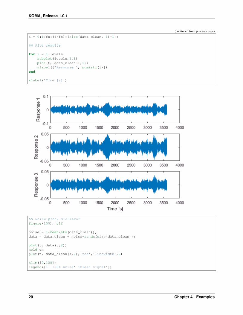
t = 0:1/fs:(1/fs)*(size(data_clean, 1)-1);
%% Plot results
for i = 1:levelssubplot(levels,1,i)plot(t, data_clean(:,i))ylabel(['Response ', num2str(i)])
end
xlabel('Time [s]')
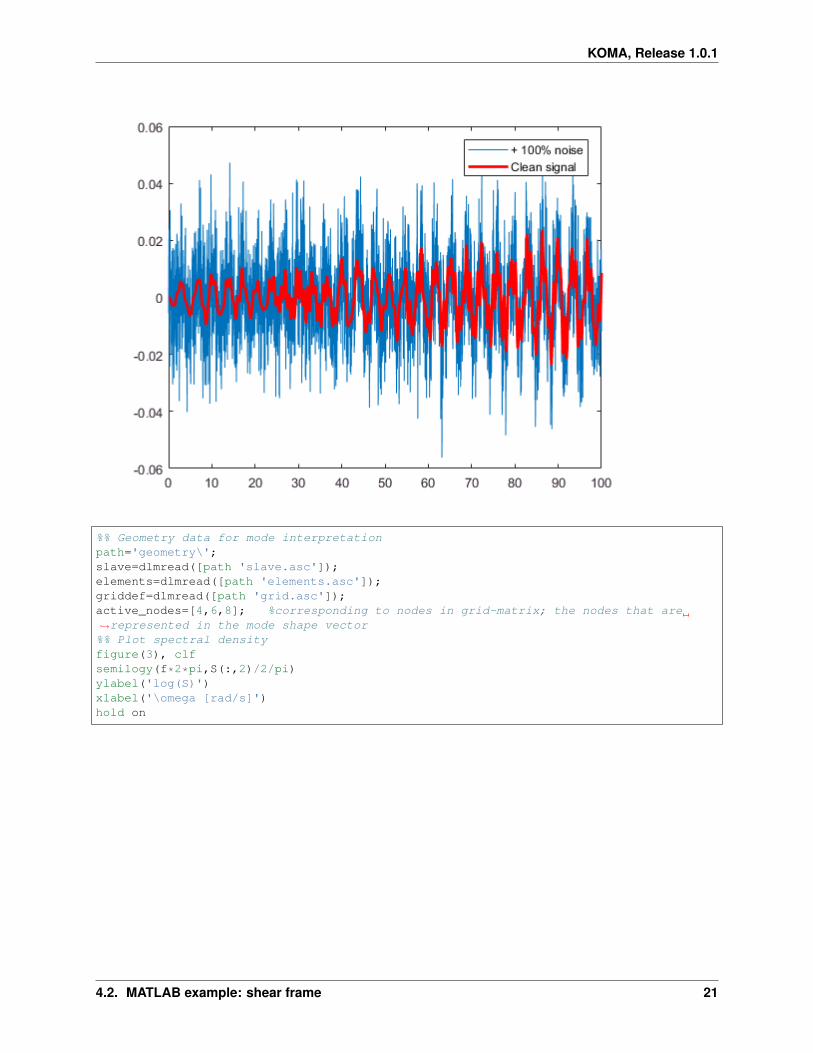
%% Noise plot, mid-levelfigure(100), clf
noise = 1*mean(std(data_clean));data = data_clean + noise*randn(size(data_clean));
plot(t, data(:,2))hold onplot(t, data_clean(:,2),'red','linewidth',2)
xlim([0,100])legend({'+ 100% noise' 'Clean signal'})
20 Chapter 4. Examples
KOMA, Release 1.0.1
%% Geometry data for mode interpretationpath='geometry\';slave=dlmread([path 'slave.asc']);elements=dlmread([path 'elements.asc']);griddef=dlmread([path 'grid.asc']);active_nodes=[4,6,8]; %corresponding to nodes in grid-matrix; the nodes that are→˓represented in the mode shape vector%% Plot spectral densityfigure(3), clfsemilogy(f*2*pi,S(:,2)/2/pi)ylabel('log(S)')xlabel('\omega [rad/s]')hold on
4.2. MATLAB example: shear frame 21

KOMA, Release 1.0.1
%% SSI runi = 20; %blockrowsorder = 2:2:50;figure(5)fs_rs = ceil(2*max(abs(lambda_ref)/2/pi));data_rs = resample(detrend(data),fs_rs,fs);% Extend data matrix to 3d (for easy plotting of mode shapes, not necessary for ssi)data_3d = zeros(size(data_rs,1),3*size(data_rs,2));data_3d(:,1:3:end) = data_rs;data_3d(:,2:3:end) = 0*data_rs;data_3d(:,2:3:end) = 0*data_rs;
[lambda,phi,order] = koma.oma.covssi(data_3d, fs_rs, i, 'order',order);
Resulting output:
*** COVARIANCE DRIVEN SSI ALGORITHM FOR OPERATIONAL MODAL ANALYSIS ***** ESTABLISHING HANKEL AND TOEPLITZ MATRICES
** Correlation estimation
** Matrix stacking
* CALCULATING SVD OF MATRICES AND CONTROLLING MAXIMUM ORDER
** Rank(D) = 60
** Maximum system order used is n_max = 50
* ESTABLISHING WEIGHTING MATRIX
* COMPUTING STATE MATRIX FROM DECOMPOSITION FOR EACH ORDER, AND ESTABLISH EIGENVALUES→˓AND EIGENVECTORS
* COMPUTATION COMPLETE!
22 Chapter 4. Examples
KOMA, Release 1.0.1
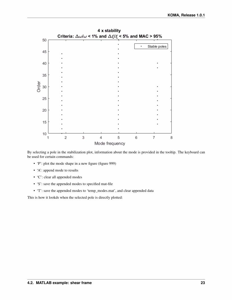
By selecting a pole in the stabilization plot, information about the mode is provided in the tooltip. The keyboard canbe used for certain commands:
• ‘P’: plot the mode shape in a new figure (figure 999)
• ‘A’: append mode to results
• ‘C’: clear all appended modes
• ‘S’: save the appended modes to specified mat-file
• ‘T’: save the appended modes to ‘temp_modes.mat’, and clear appended data
This is how it lookds when the selected pole is directly plotted:
4.2. MATLAB example: shear frame 23

KOMA, Release 1.0.1
4.3 MATLAB exaple: visualization of beam modes
See the file ./examples/matlab/beam_modes.m. The content and results of the file are reproduced in the followingsubsection.
import ../../koma.*
%% Geometry data for mode interpretationpath='geometry_beam\';slave=dlmread([path 'slave.asc']);elements=dlmread([path 'elements.asc']);griddef=dlmread([path 'grid.asc']);active_nodes=2:8; %corresponding to nodes with sensors, and thus has to match the→˓dimensions of phi (/3)
%% Plot modemode_n = 1;
x = griddef(:,2);phi_1d_all = cos(mode_n*(1-x/5) * pi/2);phi_1d_sensors = phi_1d_all(4:end);phi_3d = [phi_1d_sensors*0, phi_1d_sensors, phi_1d_sensors*0]';phi = phi_3d(:);
koma.vis.plot_mode(phi, griddef, elements, slave, active_nodes, 'labels', 'deformed')
24 Chapter 4. Examples

KOMA, Release 1.0.1
4.3. MATLAB exaple: visualization of beam modes 25

KOMA, Release 1.0.1
26 Chapter 4. Examples

CHAPTER
FIVE
LICENSING INFORMATION
Please cite both the original research paper for which the code was developed for and the the code if used in research.
The software is licensed under the MIT license:
Copyright (c) 2020 Knut Andreas Kvåle
Permission is hereby granted, free of charge, to any person obtaining a copy of this software and associ-ated documentation files (the “Software”), to deal in the Software without restriction, including withoutlimitation the rights to use, copy, modify, merge, publish, distribute, sublicense, and/or sell copies of theSoftware, and to permit persons to whom the Software is furnished to do so, subject to the followingconditions:
The above copyright notice and this permission notice shall be included in all copies or substantial portionsof the Software.
THE SOFTWARE IS PROVIDED “AS IS”, WITHOUT WARRANTY OF ANY KIND, EXPRESS ORIMPLIED, INCLUDING BUT NOT LIMITED TO THE WARRANTIES OF MERCHANTABILITY,FITNESS FOR A PARTICULAR PURPOSE AND NONINFRINGEMENT. IN NO EVENT SHALLTHE AUTHORS OR COPYRIGHT HOLDERS BE LIABLE FOR ANY CLAIM, DAMAGES OROTHER LIABILITY, WHETHER IN AN ACTION OF CONTRACT, TORT OR OTHERWISE, ARIS-ING FROM, OUT OF OR IN CONNECTION WITH THE SOFTWARE OR THE USE OR OTHERDEALINGS IN THE SOFTWARE.
27

KOMA, Release 1.0.1
28 Chapter 5. Licensing information

CHAPTER
SIX
REFERENCES
29

KOMA, Release 1.0.1
30 Chapter 6. References

CHAPTER
SEVEN
ACKNOWLEDGEMENTS
Jos van der Geest contribution to Mathworks Central File Exchange is used to produce error bars in stability plots ofMATLAB function stabplot.m.
31
KOMA, Release 1.0.1
32 Chapter 7. Acknowledgements


KOMA, Release 1.0.1
34 Chapter 8. Indices and tables

BIBLIOGRAPHY
[1] L HERMANS and H VAN DER AUWERAER. MODAL TESTING AND ANALYSIS OF STRUCTURES UN-DER OPERATIONAL CONDITIONS: INDUSTRIAL APPLICATIONS. Mechanical Systems and Signal Pro-cessing, 13(2):193–216, mar 1999. URL: http://www.sciencedirect.com/science/article/pii/S0888327098912110,doi:http://dx.doi.org/10.1006/mssp.1998.1211.
[2] Peter Van Overschee and Bart De Moor. Subspace identification for linear systems: theory, implementation, ap-plications. Kluwer Academic Publishers, Boston/London/Dordrecht, 1996.
[3] Carlo Rainieri and Giovanni Fabbrocino. Operational Modal Analysis of Civil Engineering Structures. Springer,New York, 2014.
[4] Brad A. Pridham and John C. Wilson. A study of damping errors in correlation-driven stochastic realizations usingshort data sets. Probabilistic Engineering Mechanics, 18(1):61–77, jan 2003. URL: http://www.sciencedirect.com/science/article/pii/S0266892002000425, doi:10.1016/S0266-8920(02)00042-5.
[5] Knut Andreas Kvåle, Ole Øiseth, and Anders Rønnquist. Operational modal analysis of an end-supported pontoonbridge. Engineering Structures, 148:410–423, oct 2017. URL: http://www.sciencedirect.com/science/article/pii/S0141029616307805, doi:10.1016/j.engstruct.2017.06.069.
[6] K.A. Kvåle and Ole Øiseth. Automated operational modal analysis of an end-supported pontoon bridge usingcovariance-driven stochastic subspace identification and a density-based hierarchical clustering algorithm. IAB-MAS Conference, 2020.
35

KOMA, Release 1.0.1
36 Bibliography

MATLAB MODULE INDEX
kkoma, 7koma.modal, 8koma.oma, 7koma.vis, 10
37

KOMA, Release 1.0.1
38 MATLAB Module Index

INDEX
Aanimate_mode() (in module koma.vis), 10
Ccovssi() (in module koma.oma), 7
Dddssi() (in module koma.oma), 8
Ffind_stable_poles() (in module koma.modal), 8
Kkoma (module), 7koma.modal (module), 8koma.oma (module), 7koma.vis (module), 10
Ppick_stable_modes() (in module koma.modal), 9plot_mode() (in module koma.vis), 11
Rresasref() (in module koma.modal), 10
Sstabplot() (in module koma.vis), 13
Xxmacmat() (in module koma.modal), 10
39