release 0.1.0 nikolaus sonnenschein, joão cardoso · cameo documentation, release 0.1.0 warning:...

cameo DocumentationRelease 0.1.0

Nikolaus Sonnenschein, João Cardoso

January 19, 2016

Contents

1 Table of Contents 31.1 Dependencies . . . . . . . . . . . . . . . . . . . . . . . . . . . . . . . . . . . . . . . . . . . . . . . 31.2 Installation . . . . . . . . . . . . . . . . . . . . . . . . . . . . . . . . . . . . . . . . . . . . . . . . 31.3 Getting started with cameo . . . . . . . . . . . . . . . . . . . . . . . . . . . . . . . . . . . . . . . . 51.4 Import models . . . . . . . . . . . . . . . . . . . . . . . . . . . . . . . . . . . . . . . . . . . . . . 71.5 Simulate models . . . . . . . . . . . . . . . . . . . . . . . . . . . . . . . . . . . . . . . . . . . . . 81.6 Analyzing models . . . . . . . . . . . . . . . . . . . . . . . . . . . . . . . . . . . . . . . . . . . . 101.7 Predict expression modulation targets . . . . . . . . . . . . . . . . . . . . . . . . . . . . . . . . . . 111.8 Compute knockout strategies . . . . . . . . . . . . . . . . . . . . . . . . . . . . . . . . . . . . . . . 131.9 Predict heterologous pathways . . . . . . . . . . . . . . . . . . . . . . . . . . . . . . . . . . . . . . 161.10 Parallelization . . . . . . . . . . . . . . . . . . . . . . . . . . . . . . . . . . . . . . . . . . . . . . 211.11 cameo vs. cobrapy . . . . . . . . . . . . . . . . . . . . . . . . . . . . . . . . . . . . . . . . . . . . 211.12 API . . . . . . . . . . . . . . . . . . . . . . . . . . . . . . . . . . . . . . . . . . . . . . . . . . . . 22

2 Indices and tables 27

i

cameo Documentation, Release 0.1.0

Warning: These pages are under construction. Feel free to look around ...

Cameo is a high-level python library developed to aid the strain design process in metabolic engineering projects. Thelibrary provides a modular framework of simulation methods, strain design methods, access to models, that targetsdevelopers that want custom analysis workflows.

Computationally heavy methods have been parallelized and can be run on a clusters using the IPython parallelizationframework (see example and documentation for more details). The default fallback is python’s multiprocessing library.

Furthermore, it exposes a high-level API to users that just want to compute promising strain designs.

from cameo.api import designdesign(product='L-Serine')

You got curious? Head over to try.cameo.bio and give it a try.

Contents 1

http://try.cameo.bio


2 Contents

CHAPTER 1

Table of Contents

1.1 Dependencies

Cameo has the following hard dependencies:

• [optlang](https://pypi.python.org/pypi/optlang) (for defining optimization problems)

• [numpy](http://www.numpy.org/) and [scipy](http://www.scipy.org/) (for obvious reasons)

• [inspyred](https://pypi.python.org/pypi/inspyred) (for heuristic optimizations)

• [escher](https://pypi.python.org/pypi/Escher) (for pathway visualizations)

• [blessings](https://pypi.python.org/pypi/blessings) and [IProgress](https://pypi.python.org/pypi/IProgress) (fordisplaying progress bars)

• [lazy-proxy-object](https://pypi.python.org/pypi/lazy-object-proxy) (for keeping models unevaluated)

Optionally, the following soft dependencies can be installed

• Jupyter notebook (cameo is tightly integrated with the notebook interface)

• bokeh (for plotting and showing progress)

The following dependencies are needed for development:

• [nose]() (for running unit tests)

• [rednose]() (for running unit tests)

• [coverage]() (for determining test coverage)

The following dependencies are needed for generating documentation:

• sphinx

• mock

• numpydoc

1.2 Installation

1.2.1 Setting up a virtual environment first

We highly recommended installing cameo inside a virtual environment (virtualenv). virtualenvwrapper tremendouslysimplifies using virtualenv and can easily be installed using virtualenv-burrito. Once you installed virtualenv and

3

https://pypi.python.org/pypi/optlang

http://www.numpy.org/

http://www.scipy.org/

https://pypi.python.org/pypi/inspyred

https://pypi.python.org/pypi/Escher

https://pypi.python.org/pypi/blessings

https://pypi.python.org/pypi/IProgress

https://pypi.python.org/pypi/lazy-object-proxy

https://pypi.python.org/pypi/virtualenv

https://pypi.python.org/pypi/virtualenvwrapper


https://github.com/brainsik/virtualenv-burrito



virtualenvwrapper, run

$ mkvirtualenv cameo # or whatever you'd like to call your virtual environment$ workon cameo

and then continue with the installation instructions described below.

1.2.2 Non-python dependencies

cameo relies on optlang to solve optimization problems. Currently, optlang supports either glpk (open source) or cplex(academic licenses available), which are not python tools. At least one of them has to be installed before one canproceed with the cameo installation.

GLPK

Using cameo with glpk also requires swig to be installed (in order to generate python bindings). On ubuntu (or othersimilar linux platforms) we recommend using apt-get:

$ sudo apt-get install libglpk-dev glpk-utils swig

On macs we recommend using homebrew.

$ brew install swig$ brew install glpk

CPLEX

The cplex contains a python directory (similar to IBM/ILOG/CPLEX_Studio1251/cplex/python/x86-64_osx).Inside this directory run

$ python setup.py install

to install the python bindings.

1.2.3 Normal installation

Warning: cameo is still under heavy development. We recommend installing the development version (see below)if you would like to stay up-to-date with the latest changes.

cameo can be installed using pip.

$ pip install cameo

1.2.4 Development setup

pip can also be used to install cameo directly from the github repository.

$ pip install -e git+https://github.com/biosustain/cameo.git@devel#egg=cameo

Alternatively, you can clone the repository (or your fork) and then run

4 Chapter 1. Table of Contents

https://pypi.python.org/pypi/virtualenvwrapper

https://github.com/biosustain/optlang

https://www.gnu.org/software/glpk/

http://www-01.ibm.com/software/commerce/optimization/cplex-optimizer/

https://www.gnu.org/software/glpk/

http://www.swig.org/

http://brew.sh/

http://www-01.ibm.com/software/commerce/optimization/cplex-optimizer/

https://github.com/biosustain/cameo


$ python setup.py install

From withing the cameo directory.

from pandas import optionsoptions.display.max_rows = 8

1.3 Getting started with cameo

cameo reuses and extends model data structures defined by cobrapy (COnstraints-Based Reconstruction and Analysistool for Python). So, in addition to following this quick start guide and other cameo tutorials, we encourage you toexplore cobrapy’s documentation as well.

1.3.1 Step 1: Load a model

Loading a model is easy. Just import the load_model function.

from cameo import load_model

For example, load the most current genome-scale metabolic reconstruction of Escherichia coli.

model = load_model("iJO1366")

Models, reactions, metabolites, etc., provide return HTML when evaluated in Jupyter notebooks and can thus be easilyinspected.

model

1.3.2 Step 2: Simulate a model

The model can be simulated by executing solve.

solution = model.solve()

A quick overview of the solution can be obtained in form of a pandas DataFrame (all solution objects in cameo provideaccess to data frames through a data_frame attribute).

solution

The data frame is accessible through solution.data_frame.

solution.data_frame

Data frames make it very easy to process results. For example, let’s take a look at reactions with flux != 0

solution.data_frame.query('fluxes != 0')

1.3.3 Step 3: Exploring a model

Objects—models, reactions, metabolites, genes—can easily be explored in the Jupyter notebook, taking advantage oftab completion. For example, place your cursor after the period in model.reactions. and press the TAB key. Adialog will appear that allows you to navigate the list of reactions encoded in the model.

1.3. Getting started with cameo 5

https://opencobra.github.io/cobrapy/

https://cobrapy.readthedocs.org/en/latest/cobra.core.html

http://pandas.pydata.org/pandas-docs/stable/generated/pandas.DataFrame.html


model.reactions. # place your cursor after the period and press the TAB key.

For example, you can access the E4PD (Erythrose 4-phosphate dehydrogenase) reaction in the model.

model.reactions.E4PD

Be aware though that due variable naming restrictions in Python dot notation access to reactions (and other objects)might not work in some cases.

model.reactions.12DGR120tipp

File "<ipython-input-11-fa7ea4193315>", line 1model.reactions.12DGR120tipp

^SyntaxError: invalid syntax

In these cases you need to use the model.reactions.get_by_id.

model.reactions.get_by_id('12DGR120tipp')

Metabolites are accessible through model.metabolites. For example, D-glucose in the cytosolic compartment.

model.metabolites.glc__D_c

<Metabolite glc__D_c at 0x10b7cfe48>

A list of the genes encoded in the model can be accessed via model.genes.

model.genes[0:10]

[<Gene b0929 at 0x10b8b1a20>,<Gene b1377 at 0x10b8b19b0>,<Gene b2215 at 0x10b8b19e8>,<Gene b0241 at 0x10b8b1978>,<Gene b4035 at 0x10b8b1e80>,<Gene b4033 at 0x10b8b1e10>,<Gene b4032 at 0x10b8b1e48>,<Gene b4034 at 0x10b8b1dd8>,<Gene b4036 at 0x10b8b1ef0>,<Gene b4213 at 0x10b8b89b0>]

A few additional attributes have been added that are not available in a cobrapy model. For example, exchange reactionsthat allow certain metabolites to enter or leave the model can be accessed through model.exchanges.

model.exchanges[0:10]

[<Reaction DM_4CRSOL at 0x107773da0>,<Reaction DM_5DRIB at 0x107773f60>,<Reaction DM_AACALD at 0x10a4ae5f8>,<Reaction DM_AMOB at 0x10a4ae630>,<Reaction DM_MTHTHF at 0x10ae32d30>,<Reaction DM_OXAM at 0x10ae329e8>,<Reaction EX_12ppd__R_e at 0x10ae32940>,<Reaction EX_12ppd__S_e at 0x10ae32c18>,<Reaction EX_14glucan_e at 0x10ae32fd0>,<Reaction EX_15dap_e at 0x10ae32ba8>]

Or, the current medium can be accessed through model.medium.




model.medium

It is also possible to get a list of essential reactions ...

model.essential_reactions()[0:10]

[<Reaction DM_4CRSOL at 0x107773da0>,<Reaction DM_5DRIB at 0x107773f60>,<Reaction DM_AMOB at 0x10a4ae630>,<Reaction DM_MTHTHF at 0x10ae32d30>,<Reaction Ec_biomass_iJO1366_core_53p95M at 0x10ae32c50>,<Reaction EX_ca2_e at 0x10ae38630>,<Reaction EX_cl_e at 0x10ae38828>,<Reaction EX_cobalt2_e at 0x10ae38908>,<Reaction EX_cu2_e at 0x10ae38b38>,<Reaction EX_glc_e at 0x10ae45b38>]

... and essential genes.

model.essential_genes()[0:10]

[<Gene b0029 at 0x10b998048>,<Gene b2320 at 0x10bb10080>,<Gene b0175 at 0x10b9840b8>,<Gene b2530 at 0x10ba580b8>,<Gene b0639 at 0x10bad8240>,<Gene b0025 at 0x10b9dc278>,<Gene b3807 at 0x10ba58278>,<Gene b3196 at 0x10b9482e8>,<Gene b3041 at 0x10b984438>,<Gene b3939 at 0x10bb73550>]

from pandas import optionsoptions.display.max_rows = 8

1.4 Import models

1.4.1 Import models from different file formats

pass

1.4.2 Models on the internet

In the previous chapter we showed how to to use load_model to import a model by ID. But where did themodel come from? Cameo has currently access to two model repositories on the internet, http://bigg.ucsd.edu andhttp://darwin.di.uminho.pt/models.

Cameo also has the ability to load the model from the internet. To data

from cameo import models

models.index_models_bigg()

1.4. Import models 7

http://bigg.ucsd.edu

http://darwin.di.uminho.pt/models


from pandas import optionsoptions.display.max_rows = 8from cameo import load_modelmodel = load_model("iJO1366")

1.5 Simulate models

cameo uses and extends the model data structures defined by cobrapy, our favorite COnstraints-Based Reconstructionand Analysis tool for Python. cameo is thus 100% compatible with cobrapy. For efficiency reasons, however, cameoimplements its own simulation methods that take advantage of a more advanced solver interface.

1.5.1 Primer: Constraint-Based Modeling

Constraint-based modeling is a powerful modeling framework for analyzing metabolism on the genome scale (Mc-Closkey et al., 2013). For a model that encompasses 𝑛 reactions that involve 𝑚 metabolites, S is a matrix of dimension𝑚× 𝑛 that encodes the stoichiometry of the metabolic reaction system; it is usually referred to as stoichiometric ma-trix. Assuming that the system is in a steady state—the concentration of metabolites are constant—the system offlux-balances can be formulated as

Sv = 0 , (1.1)

where v is the vector of flux rates. With the addition of a biologically meaningful objective, flux capacity constraints,information about the reversibility of reactions under physiological conditions, an optimization problem can be for-mulated that can easily be solved using linear programming.

, e.g., maximimization of biomass production,Given the maximization of growth rate as one potential biological ob-jective 𝑣𝑏𝑖𝑜𝑚𝑎𝑠𝑠, i.e., the flux of an artificial reaction that consumes biomass components in empirically determinedproportions, and assuming that the cell is evolutionary optimized to achieve that objective, and incorporating knowl-edge about reaction reversibility, uptake and secretion rates, and maximum flux capacities in the form of lower anduppers bounds (v𝑙𝑏 and v𝑢𝑏) on the flux variables v, one can formulate and solve an optimization problem to identifyan optimal set of flux rates using flux balance analysis (FBA):

𝑀𝑎𝑥 𝑍𝑜𝑏𝑗 = c𝑇v (1.2)s.t. Sv = 0(1.3)

v𝑙𝑏 ≤ v ≤ v𝑢𝑏 .(1.4)

1.5.2 Flux Balance Analysis

In cameo, flux balance analysis can be performed with the function fba.

from cameo import fbafba_result = fba(model)

Basically, fba calls model.solve() and wraps the optimization solution in a FluxDistributionResultobject. The maximum objective values (corresponding to a maximum growth rate) can obtained througresult.objective_value.

fba_result.objective_value

0.9823718127269799



http://www.ncbi.nlm.nih.gov/pubmed/23632383


https://en.wikipedia.org/wiki/Linear_programming


1.5.3 Parsimonious Flux Balance Analysis

Parsimonious flux balance analysis (Lewis et al., 2010), a variant of FBA, performs FBA in in a first step to determinethe maximum objective value 𝑍𝑜𝑏𝑗 , fixes it in form of an additional model constraint (c𝑇v ≥ 𝑍𝑜𝑏𝑗), and then minimizesin a second optimization the 𝐿1 norm of v. The assumption behind the pFBA is that cells try to minimize fluxmagnitude as well in order to keep the costs of protein low.

𝑀𝑎𝑥 |v| (1.5)s.t. Sv = 0(1.6)

c𝑇v ≥ 𝑍𝑜𝑏𝑗(1.7)v𝑙𝑏 ≤ v ≤ v𝑢𝑏 .(1.8)

In cameo, pFBA can be performed with the function pfba.

from cameo import pfbapfba_result = pfba(model)

The objective_function value is |v| ...

pfba_result.objective_value

699.0222751839377

... whis is significantly smaller than flux vector of the original FBA solution.

abs(fba_result.data_frame.flux).sum()

764.91487969777245

1.5.4 Setp 2: Simulate knockouts phenotypes

Although PFBA and FBA can be used to simulate the effect of knockouts, other methods have been proven morevaluable for that task: MOMA and ROOM. In cameo we implement a linear version of MOMA.

Simulating knockouts:

• Manipulate the bounds of the reaction (or use the shorthand method knock_out)

model.reactions.PGI

model.reactions.PGI.knock_out()model.reactions.PGI

• Simulate using different methods:

%timefba_knockout_result = simulation.fba(model)fba_knockout_result[model.objective]

CPU times: user 2 µs, sys: 0 ns, total: 2 µsWall time: 5.01 µs

0.905983

1.5. Simulate models 9



pfba_knockout_result = simulation.pfba(model)pfba_knockout_result[model.objective]

0.905983

MOMA and ROOM relly on a reference (wild-type) flux distribution and we can use the one previously computed.

Parsimonious FBA references seem to produce better results using this methods

lmoma_result["2 * EX_glc_lp_e_rp_"]

-18.7358

%timelmoma_result = simulation.lmoma(model, reference=pfba_result.fluxes)lmoma_result[model.objective]

CPU times: user 2 µs, sys: 1 µs, total: 3 µsWall time: 5.01 µs

0.791393

%timeroom_result = simulation.room(model, reference=pfba_result.fluxes)room_result[model.objective]

CPU times: user 2 µs, sys: 1 µs, total: 3 µsWall time: 5.01 µs

0.887440

room_result

<cameo.core.result.FluxDistributionResult at 0x10aa75b50>

1.6 Analyzing models

computer aided metabolic engineering and optimization

cameo uses and extends the model data structures defined by cobrapy, our favorite COnstraints-Based Reconstructionand Analysis tool for Python. cameo is thus 100% compatible with cobrapy. For efficiency reasons though cameoimplements its own analysis methods that take advantage of a more advanced solver interface.

from cameo import modelsmodel = models.bigg.e_coli_core

1.6.1 Flux Variability Analysis

Flux variability analysis (FVA) enables the computation of lower and upper bounds of reaction fluxes.

from cameo import flux_variability_analysis

fva_result = flux_variability_analysis(model, reactions=[model.reactions.PGI, model.reactions.EX_glc_e])fva_result.data_frame




One very useful application of FVA is determining if alternative optimal solution exist.

fva_result = flux_variability_analysis(model, reactions=[model.reactions.PGI, model.reactions.EX_glc_e],fraction_of_optimum=1.)

fva_result.data_frame

1.6.2 Phenotpic Phase Plane

from cameo import phenotypic_phase_plane

model.reactions.EX_o2_e.lower_bound = -10result = phenotypic_phase_plane(model,

variables=[model.reactions.Biomass_Ecoli_core_w_GAM],objective=model.reactions.EX_succ_e,points=10)

result.plot(height=400)

result.data_frame

1.7 Predict expression modulation targets

1.7.1 Differential flux variability analysis

from cameo import modelsfrom cameo.flux_analysis.analysis import phenotypic_phase_planefrom cameo.strain_design.deterministic import DifferentialFVA

E. coli model and succinate production

Load the E. coli core model.

model = models.bigg.e_coli_core

The production envelope looks like this.

production_envelope = phenotypic_phase_plane(model,variables=[model.reactions.Biomass_Ecoli_core_w_GAM],objective=model.reactions.EX_succ_e)

production_envelope.plot()

Set up a model that represents a reference state (in this case a model with a constrained growth rate).

reference_model = model.copy()biomass_rxn = reference_model.reactions.Biomass_Ecoli_core_w_GAMbiomass_rxn.lower_bound = 0.3target = reference_model.reactions.EX_succ_etarget.lower_bound = 2

Set up the differential flux variability analysis strain design method.

1.7. Predict expression modulation targets 11


diffFVA = DifferentialFVA(design_space_model=model,reference_model=reference_model,objective=target,variables=[biomass_rxn],normalize_ranges_by=biomass_rxn,points=10)

diffFVA = DifferentialFVA(model, model.reactions.EX_succ_e, points=20)

Run differential flux variability analysis (only on the surface of the production envelope)

result = diffFVA.run(surface_only=True, improvements_only=True)result.plot()

result.display_on_map("iJO1366.Central metabolism")

<IPython.core.display.Javascript object>





















1.8 Compute knockout strategies

import cameofrom cameo import modelsfrom cameo.strain_design.heuristic import GeneKnockoutOptimization, ReactionKnockoutOptimizationfrom cameo.strain_design.heuristic.objective_functions import biomass_product_coupled_yield, product_yield, number_of_knockoutsfrom cameo.flux_analysis.simulation import fbafrom cameo.parallel import SequentialViewimport inspyred

model = models.bigg.e_coli_core

objective1 = biomass_product_coupled_yield(model.reactions.Biomass_Ecoli_core_w_GAM,model.reactions.EX_ac_e,model.reactions.EX_glc_e)

objective2 = number_of_knockouts()objective = [objective1, objective2]

ko = GeneKnockoutOptimization(model=model,simulation_method=fba,objective_function=objective,heuristic_method=inspyred.ec.emo.NSGA2,seed=1234)

results = ko.run(max_evaluations=3000, popuplation_size=100, view=SequentialView())

Starting optimization at Fri, 17 Jul 2015 13:53:04

Using saved session configuration for http://localhost:5006/To override, pass 'load_from_config=False' to Session

/Users/niko/.virtualenvs/cameo_py3/lib/python3.4/site-packages/bokeh/session.py:319 [1;31mUserWarning[0m: You need to start the bokeh-server to see this example.











1.8. Compute knockout strategies 13




























Finished after 00:00:16

results

1.8. Compute knockout strategies 15


from IPython.display import displayimport re

1.9 Predict heterologous pathways

from cameo import modelsfrom cameo.strain_design import pathway_prediction

import logginglogging.getLogger('cameo').setLevel(logging.DEBUG)

predictor.mapping['atp']

'MNXM3'

predictor.adpater_reactions

[]

predictor.model.solver.configuration.verbosity = 3

pathways = predictor.run(product="L-Serine", max_predictions=1)

INFO:cameo.strain_design.pathway_prediction:Predicting pathway No. 1

Found incumbent of value 2513.000000 after 0.16 sec. (31.18 ticks)MIP emphasis: balance optimality and feasibility.MIP search method: dynamic search.Parallel mode: deterministic, using up to 4 threads.Root relaxation solution time = 0.44 sec. (147.56 ticks)

Nodes Cuts/Node Left Objective IInf Best Integer Best Bound ItCnt Gap

* 0+ 0 2513.0000 0.0000 100.00%

* 0+ 0 59.0000 0.0000 100.00%

* 0+ 0 35.0000 0.0000 100.00%0 0 0.0003 3 35.0000 0.0003 1020 100.00%

* 0+ 0 3.0000 0.0003 99.99%0 0 1.0002 2 3.0000 Covers: 1 1021 66.66%0 0 1.0002 4 3.0000 Covers: 1 1028 66.66%0 0 1.0002 4 3.0000 Covers: 1 1030 66.66%0 0 cutoff 3.0000 1.0002 1030 66.66%

Elapsed time = 1.18 sec. (260.74 ticks, tree = 0.00 MB, solutions = 4)

Cover cuts applied: 3

Root node processing (before b&c):Real time = 1.18 sec. (261.05 ticks)

Parallel b&c, 4 threads:Real time = 0.07 sec. (1.53 ticks)Sync time (average) = 0.00 sec.Wait time (average) = 0.00 sec.

------------Total (root+branch&cut) = 1.25 sec. (262.57 ticks)



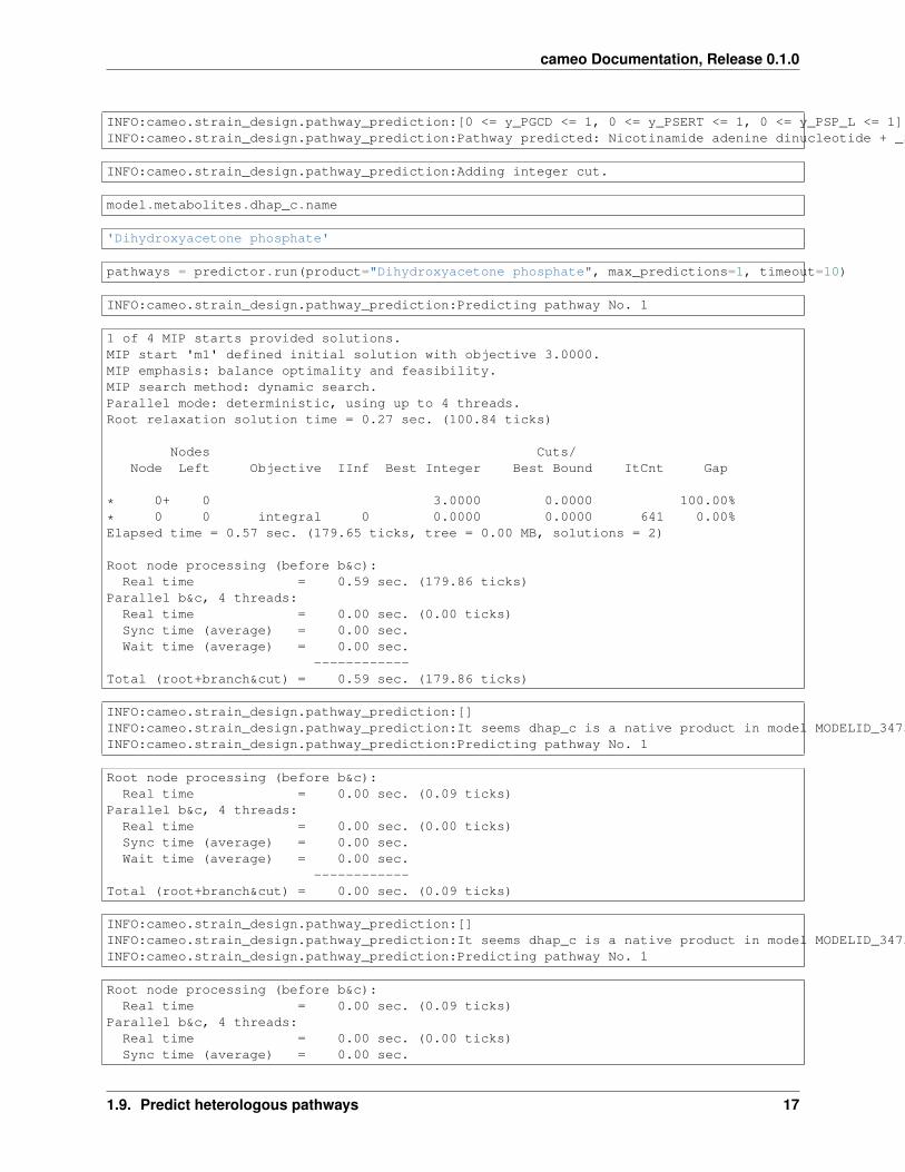
INFO:cameo.strain_design.pathway_prediction:[0 <= y_PGCD <= 1, 0 <= y_PSERT <= 1, 0 <= y_PSP_L <= 1]INFO:cameo.strain_design.pathway_prediction:Pathway predicted: Nicotinamide adenine dinucleotide + _3-Phospho-D-glycerate --> 3-Phosphohydroxypyruvate + Nicotinamide adenine dinucleotide - reduced + H+ 3-Phosphohydroxypyruvate + L-Glutamate --> _2-Oxoglutarate + O-Phospho-L-serine H2O + O-Phospho-L-serine --> L-Serine + Phosphate

INFO:cameo.strain_design.pathway_prediction:Adding integer cut.

model.metabolites.dhap_c.name

'Dihydroxyacetone phosphate'

pathways = predictor.run(product="Dihydroxyacetone phosphate", max_predictions=1, timeout=10)

INFO:cameo.strain_design.pathway_prediction:Predicting pathway No. 1

1 of 4 MIP starts provided solutions.MIP start 'm1' defined initial solution with objective 3.0000.MIP emphasis: balance optimality and feasibility.MIP search method: dynamic search.Parallel mode: deterministic, using up to 4 threads.Root relaxation solution time = 0.27 sec. (100.84 ticks)

Nodes Cuts/Node Left Objective IInf Best Integer Best Bound ItCnt Gap

* 0+ 0 3.0000 0.0000 100.00%

* 0 0 integral 0 0.0000 0.0000 641 0.00%Elapsed time = 0.57 sec. (179.65 ticks, tree = 0.00 MB, solutions = 2)




INFO:cameo.strain_design.pathway_prediction:[]INFO:cameo.strain_design.pathway_prediction:It seems dhap_c is a native product in model MODELID_3473243. Let's see if we can find better heterologous pathways.INFO:cameo.strain_design.pathway_prediction:Predicting pathway No. 1






Parallel b&c, 4 threads:Real time = 0.00 sec. (0.00 ticks)Sync time (average) = 0.00 sec.

1.9. Predict heterologous pathways 17


Wait time (average) = 0.00 sec.------------

Total (root+branch&cut) = 0.00 sec. (0.09 ticks)




































1.9. Predict heterologous pathways 19

















tmp = pathways.pathways[0]

tmp.adapters

[]

predictor.model.metabolites.ser__L_c.name



'ser__L_c'

predictor.run()

model = models.bigg.iMM904

predictor = pathway_prediction.PathwayPredictor(model=model, compartment_regexp=re.compile(".*_c$"))

INFO:cameo.strain_design.pathway_prediction:Loading default universal model.INFO:cameo.strain_design.pathway_prediction:Trying to set solver to cplex to speed up pathway predictions.INFO:cameo.strain_design.pathway_prediction:Adding reactions from universal model to host model.

pathways = predictor.run(product="vanillin", max_predictions=5)

from cameo import phenotypic_phase_planefrom cameo.util import TimeMachinefrom cameo.visualization.plotting import Grid

with Grid(nrows=3) as grid:for i, pathway in enumerate(pathways):

with TimeMachine() as tm:pathway.plug_model(model, tm=tm)ppp = phenotypic_phase_plane(model, variables=[model.reactions.biomass_SC5_notrace], objective=pathway.product)ppp.plot(grid=grid, width=450, height=350, title="Pathway %i" % (i+1), axis_font_size="12pt")

1.10 Parallelization

Most methods in cameo can be parallelized using views.

1.11 cameo vs. cobrapy

1.11.1 Importing a model

cobrapy (load a model in SBML format):

from cobra.io import read_sbml_modelmodel = read_sbml_model('path/to/model.xml')

cameo (load models from different formats):

from cameo import load_model# read SBML modelmodel = load_model('path/to/model.xml')# ... or read a pickled modelmodel = load_model('path/to/model.pickle')# ... or just import a model by ID from http://darwin.di.uminho.pt/modelsiAF1260 = load_model('iAF1260')

1.11.2 Solving models

cobrapy:

1.10. Parallelization 21


solution = model.optimize()if solution.status == 'optimal':

# proceed

try:solution = model.solve()

except cameo.exceptions.SolverError:print "A non-optimal solution was returned by the solver"

else:# proceed

It is important to note that cameo models maintain optimize to maintain compatibility with cobrapy but we dis-courage its use.

1.12 API

1.12.1 cameo package

Subpackages

cameo.api package

Submodules

cameo.api.designer module

cameo.api.hosts module

cameo.api.products module

Module contents

cameo.core package

Submodules

cameo.core.reaction module

cameo.core.result module

cameo.core.solution module

cameo.core.solver_based_model module

Module contents



cameo.data package

Submodules

cameo.data.metanetx module

Module contents

cameo.flux_analysis package

Submodules

cameo.flux_analysis.analysis module

cameo.flux_analysis.simulation module

cameo.flux_analysis.util module

Module contents

cameo.models package

Submodules

cameo.models.universal module

cameo.models.webmodels module

Module contents

cameo.network_analysis package

Submodules

cameo.network_analysis.networkx_based module

cameo.network_analysis.util module

Module contents

1.12. API 23


cameo.strain_design package

Subpackages

cameo.strain_design.deterministic package

Submodules

cameo.strain_design.deterministic.flux_variability_based module

Module contents

cameo.strain_design.heuristic package

Submodules

cameo.strain_design.heuristic.archivers module

cameo.strain_design.heuristic.decoders module

cameo.strain_design.heuristic.generators module

cameo.strain_design.heuristic.genomes module

cameo.strain_design.heuristic.metrics module

cameo.strain_design.heuristic.objective_functions module

cameo.strain_design.heuristic.observers module

cameo.strain_design.heuristic.optimization module

cameo.strain_design.heuristic.plotters module

cameo.strain_design.heuristic.stats module

cameo.strain_design.heuristic.variators module

Module contents

cameo.strain_design.pathway_prediction package



Submodules

cameo.strain_design.pathway_prediction.pathway_predictor module

cameo.strain_design.pathway_prediction.util module

Module contents

Module contents

cameo.ui package

Module contents

cameo.visualization package

Submodules

cameo.visualization.escher_ext module

cameo.visualization.plotting module

cameo.visualization.visualization module

Module contents

Submodules

cameo.config module

cameo.exceptions module

cameo.io module

cameo.parallel module

cameo.util module

Module contents

1.12. API 25

CHAPTER 2

Indices and tables

• genindex

• modindex

• search

27

release 0.1.0 nikolaus sonnenschein, joão cardoso · cameo documentation, release 0.1.0 warning:...

Documents