relative versus absolute speed of adjustment in...

Experimental Economics, 6:181–207 (2003)c© 2003 Economic Science Association

Relative versus Absolute Speed of Adjustmentin Strategic Environments: Responder Behaviorin Ultimatum Games

DAVID J. COOPERCase Western Reserve University

NICK FELTOVICHUniversity of Houston

ALVIN E. ROTHHarvard University

RAMI ZWICKHong Kong University of Science and Technology

Abstract

Learning models predict that the relative speed at which players in a game adjust their behavior has a criticalinfluence on long term behavior. In an ultimatum game, the prediction is that proposers learn not to make smalloffers faster than responders learn not to reject them. We experimentally test whether relative speed of learninghas the predicted effect, by manipulating the amount of experience accumulated by proposers and responders. Theexperiment allows the predicted learning by responders to be observed, for the first time.

Keywords: Game Theory, learning, bargaining

JEL Classification: C7, C9, D83

1. Introduction

There’s an old joke about two men awakened by a bear while camping in the woods. Onestarts putting on his running shoes, and the other says, “A man can’t outrun a bear.” Thefirst man responds, “I don’t have to outrun the bear, I just have to outrun you.”

The point is that relative speed sometimes matters as much as absolute speed. This is alsoa robust prediction of models of learning in strategic environments. How a player learns toadjust his behavior, and how quickly, depends on what the other players are doing, and onhow quickly they are changing their behavior.

The advantage of learning theories over other kinds of theories is clearest for games inwhich players’ behavior changes a great deal over time, but does so slowly. For other kindsof games, namely games in which behavior very quickly converges to some stable behavior,or (especially) games in which players’ behavior changes little over time, it is easy to see

182 COOPER ET AL.

the appeal of theories that de-emphasize learning. The aim of the present paper is to showthat even in games of this latter kind, in which behavior appears to change only slowly if atall, the relative speed of learning may play a critical role in determining what behavior isobserved.

Roth and Erev (1995) showed that very simple learning models could qualitatively trackexperimentally observed behavior both in games in which behavior quickly converged to a(perfect) equilibrium and in games in which it did not, for games with similar equilibriumpredictions. Erev and Roth (1998) found that closely related learning models could predictbehavior in real time, i.e. they could approximate the speed and magnitude of players’adjustments in their behavior as they gained experience with games. The success of thelearning models in these papers rests not so much on their ability to explain behavior in anysingle game, but rather on their ability to provide a unified theory of behavior across a widevariety of games that induce vastly different behavior.

Perhaps the most surprising result in Roth and Erev (1995) is the explanation of behaviorin the ultimatum game through the use of a learning model. This simple bargaining gameis among the most studied games in experimental economics.1 It is a two player gamebetween a “proposer,” who proposes how to divide a fixed sum between the two players,and a “responder,” who either accepts the proposed division, in which case the proposedsplit is implemented, or rejects it, in which case both players earn zero. When both playersevaluate outcomes only in terms of their own payoff, the perfect equilibrium of this gameis for the proposer to offer the smallest feasible positive amount to the responder, andfor the responder to accept. The experimental results, in contrast, consistently show thatsmall offers are made rarely, and are frequently rejected when made. The most commonoutcome is that the proposer offers the responder something in the range of 40–50%, andthe responder accepts.

Reinforcement models of learning explain the robust experimental results in terms of therelative speed of learning that the game induces between the two kinds of players.2 Thesetheories predict that a responder who receives a very small offer adjusts his behavior little,after either accepting or rejecting it, because (since it is a small offer) accepting it gives onlyslightly greater reinforcement than rejecting it. However a proposer who makes a moderateoffer and has it accepted reaps a large reward, unlike a proposer who makes a small offer andhas it rejected. Thus proposers learn not to make small offers much faster than responderslearn not to reject them. And, once proposers stop making small offers (or make them veryrarely), there is little further opportunity for responders to learn not to reject them. So ifplayers begin with somewhat diffuse propensities over what offers to make and accept, thelearning dynamics reproduce the experimentally observed behavior.

However, there exists little experimental evidence that the behavior of responders changesover time. This is not entirely unexpected, since the learning models predict that learning byresponders will be very much slower than that of proposers, but it presents a critical empiricalchallenge to learning theories. These theories posit that the responders and proposers learnin precisely the same way, even though the game causes them to learn at different speeds.While learning models appear to explain a wide range of strategic behavior in very differentgames,3 the failure to detect responder learning in ultimatum games raises the question ofwhether this success is somehow accidental. Indeed, alternative theories have been presented

RELATIVE VERSUS ABSOLUTE SPEED OF ADJUSTMENT 183

for the ultimatum game, in which players have unchanging preferences over distributionsof outcomes rather than just their own payoffs (a “taste for fairness,”), that also capture themain features of ultimatum game data.4 Unlike learning theories, these theories predict thatthe behavior of responders will not change over time (see e.g. Ochs and Roth, 1988; Bolton,1991; Bolton and Ockenfels, 2000; Fehr and Schmidt, 1999; Rabin 1993).5 In some waysthis approach seems more natural than learning theories, since responders in the ultimatumgame are not faced with any strategic complexities that can only slowly be learned. Howeversince quite a range of learning theories also predict the experimental results, the existingdata cannot help determine if the conceptual explanation of responder behavior embodiedin the learning models has predictive power beyond that of alternative theories.

The present paper reports an experiment designed to directly test the learning theorypredictions about responder behavior in ultimatum games, by examining if the relativespeeds of learning by proposers and responders have the predicted effect. The design of theexperiment rests heavily on the learning model. That is, the design is intended to make it easyto see learning on the part of responders if it arises in just the way that the learning modelpredicts, as a function of the simultaneous learning being experienced by the proposers.

Specifically, we will seek to directly influence the relative speeds of learning by varyingthe amount of experience that proposers and responders obtain. In one condition of ourexperiment, called the 1 × 1 condition, responders and proposers will play the ultimatumgame equally often. In the other condition, called the 2 × 1 condition, responders will playtwice as often as proposers. For example, a responder playing his tenth ultimatum gamewill be receiving a proposal from a proposer playing his fifth game. The reinforcementlearning model predicts that, because a responder in the 2 × 1 condition is playing lessexperienced proposers, he will receive more low offers, and learn more quickly to acceptthem, compared to the 1 × 1 condition in which responders and proposers acquire equalexperience. Therefore rejection rates should be lower in the 2 × 1 treatment.6

The present experiment is designed so that, if the learning models are correct aboutthe kind of learning going on in ultimatum games, it will have enhanced power to detectthe learning of responders. The experimental results are consistent with the predictionsof the learning model. As predicted by the learning model, rejection rates are significantlylower in the 2×1 treatment than in the 1×1 treatment. Beyond predicting a treatment effect,the learning model also predicts a mechanism underlying the treatment effect. Respondersin the 2×1 treatment should receive more low offers, and therefore have more opportunitiesto learn to accept low offers. When we econometrically control for the proportion of lowoffers received by the responders, we find that the treatment effect vanishes. The results ofour experiment thus find the predicted effect, for the predicted reason.

In summary, the behavior of responders in the ultimatum game presents a test of theapparent generality of theories of learning in games. Alternative explanations of observedbehavior in ultimatum games have been proposed that do not involve any learning, but rathersuppose that responders have unchanging preferences for fairness. Since existing experi-mental results are consistent with both sorts of theories, we have designed an experimentthat should make it easy to detect learning by responders if they are learning in exactlythe same fashion as proposers. Our experimental results are consistent with the predictionsof reinforcement learning models. In particular, we can predict changes in responders’

184 COOPER ET AL.

behavior as we manipulate the relative speeds of learning by proposers and responders.Thus the learning models, which explain the easily observed features of the ultimatumgame in terms of the relative speed of learning on each side of the game, also give usthe ability to predict even very subtle effects having to do with the relative speed oflearning.

2. Experimental methods

We ran sixteen experimental sessions, consisting of eight 1×1 sessions (with equal numbersof proposers and responders) and eight 2 × 1 sessions (with twice as many proposers asresponders). A total of 250 subjects participated in the sixteen sessions, split into 112subjects in 1 × 1 sessions and 138 subjects in 2 × 1 sessions. Subjects were primarilyundergraduates at the University of Pittsburgh. No subject participated in more than onesession.

In each session, subjects were randomly assigned to computer terminals; the assignedterminal determined the role of the subject (proposer or responder). Subjects remained inthe same role throughout a session. Subjects were handed written instructions and giventime to read them. The instructions were then read aloud by a monitor in order for the rulesof the game to be common knowledge. Subjects’ questions were also answered at this time.

Most sessions consisted of 50 periods of play. One session was cut short after 40 periodsdue to a computer crash. Two sessions that finished early were run for an additional 10periods in order to observe the further development of play. Subjects were not told inadvance how many periods would be played, but they did know that the session would lastno longer than 2 hours.

The sequence of events in a period was as follows. First, proposers and responders wererandomly matched. The matching algorithm prohibited players from being matched to thesame counterpart in two successive periods; otherwise, all matchings were equally likely.Matchings were anonymous. Next, proposers were prompted to choose an offer. Offerswere constrained to be whole dollar amounts between $1.00 and $10.00 inclusive (out of$10.00). After offers were made and verified, each responder was shown the offer of hisproposer and prompted to choose a response (accept or reject). After responses were madeand verified, players were shown the result of play in that period (own action, other player’saction, own payoff and other’s payoff) and prompted to press a key to continue. After allsubjects had pressed the key, the next period began. Each subject’s computer screen kepttrack of his or her recent history of play.

At the end of a session, one period was randomly chosen and subjects earned their payoff(in dollars) for that period in addition to a show-up fee of $5.00.7

In the 1 × 1 condition, all responders and proposers played in every period. In the 2 × 1condition, all responders played every period while proposers only played every otherperiod. More specifically, proposers were split into two groups with one group playing onlyodd numbered periods and the other playing only even numbered periods. This treatmentwas designed to make the responders relatively more experienced than the proposers. Forinstance, when a responder plays his tenth ultimatum game he is matched with a proposerplaying only his fifth game.


To maximize the likelihood that any observed differences in subject behavior in the twocells were due only to changes in the relative frequency of play, we made it difficult forproposers in the 2 × 1 sessions to realize that they were playing in only every second period.The instructions did not make any mention of period numbers, so we could unobtrusivelyvary the number of periods that different subjects played, without the use of deception. Allreferences to “period” numbers on a subject’s screen were in the subject’s own time (so thatin a 2 × 1 session, what was period 20 to a responder would be period 10 to a proposer).

3. The reinforcement learning model: Description and predictions

In this section, we use simulations based on a reinforcement learning model to generatepredictions for this experiment. More precisely, each individual will be modeled as a rein-forcement learner, and the predictions of the learning model for the current experiment willbe developed by running computational simulations of the experiment in which simulatedplayers will be matched as in the actual experiment. Our goal is not to find the learningmodel that best fits the data from this experiment, but rather to develop a simple model thatallows us to robustly predict outcomes for this (and other) experiments.

To maintain comparability with the analysis in Roth and Erev (1995), we use one of theirsimple models for the simulations.8 The technical details of the reinforcement learningmodel and the simulations are contained in Appendix A of this paper. To understand thegist of the material, however, a brief intuitive description of the model and a summary ofhow it was implemented for the simulations will suffice. The reinforcement learning modelformalizes two basic psychological principles. First, strategies that do better are playedmore frequently over time. Second, the rate of adjustment slows down over time. These twoprinciples, known respectively as the “Law of Effect” (Thorndike, 1898) and the “PowerLaw of Practice” (Blackburn, 1936), have been validated by numerous experiments.

To formalize these two “laws,” the reinforcement learning model assumes that playersplace a weight, known as a propensity, upon each of the available strategies. The probabilityof a strategy being chosen is proportional to its propensity. The central feature of the model ishow the propensities are updated following each play. In the simplest version of the model,the propensity for the strategy that was just used is updated (reinforced) by adding therealized payoff to the propensity while the propensities for other strategies are unaffected.We study a version of the model that includes “forgetting”—all propensities are discountedby a fixed factor prior to the updating. Intuitively, this modification to the model puts greaterweight on relatively recent experiences.9

Because the amount of reinforcement a strategy receives after being played depends onthe realized payoff, strategies that yield higher expected payoffs will also receive greaterreinforcements. It follows that the reinforcement learning model obeys the Law of Effect.As long as the rate of forgetting is not too great, the total sum of propensities will growover time. Since the size of payoffs (and hence reinforcements) is not changing over time,it follows that the reinforcement learning model will follow the Power Law of Practice withlearning curves becoming flatter over time.

In implementing the reinforcement learning model for the simulations, we mimic theexperiments as much as possible. Each (simulated) proposer is allowed to use the ten

186 COOPER ET AL.

offers available in the actual experiment. For simplicity, we restrict responders to the use ofcutoff strategies, where a responder’s cutoff specifies the lowest offer that play is willingto accept.10 Higher cutoffs correspond to tougher behavior by responders. The restrictionto cutoff strategies gives the responders ten available strategies, like the proposers. For allsimulations there were 10 responders. For simulations of the 1 × 1 treatment there wereten proposers, with this doubled to twenty proposers for simulations of the 2 × 1 treatment.These numbers are similar in scale to the numbers of subjects in our sessions. As in theactual experiments, the simulated proposers play in every period for the 1 × 1 simulationsand alternate periods in the 2 × 1 simulations. Simulated subjects were randomly matchedas in the experiments. All of the simulations were run for 50 periods, the modal numberof periods in the actual experiments. This allows us only 25 periods to compare proposers’behavior between the two treatments.

Because our goal is to predict behavior in our experiments, we did not engage in astatistical exercise to find the best possible set of parameters either for these experimentsor some previously published experiment.11 Instead, we restrict the initial values of thepropensities to generate a fixed distribution of strategies similar to those typically observedin ultimatum game experiments. We also pick plausible values for the strength of the initialpropensities and the rate of forgetting, the parameters that govern the speed of learning,to serve as a baseline.12 After generating predictions for the baseline parameter values,we then vary the strength of the initial propensities and the rate of forgetting to study therobustness of these predictions. For all sets of parameters we ran 10,000 simulations, so ourpredictions are unlikely to depend on the particulars of what random numbers were drawnfor the simulations.

The top two panels of figure 1summarize the results of the baseline simulations while thebottom two panels compare the predicted treatment effects across a variety of parametervalues.

The top left panel in figure 1 shows the average offer over the 10,000 baseline simulationsfor each treatment. The periods shown on the x-axis are given from the proposer’s point ofview. Thus, the 50th period of a 2 × 1 simulation is shown as the 25th proposer-period, sinceit is only the 25th time the proposers have made a decision. For both treatments, the averageoffer rises over time. This increase does not reflect some general theoretical property ofthe reinforcement learning model, but instead depends on the initial propensities. Sincethe initial offers are slightly lower on average than the best response to responders’ initialbehavior, the average offer must rise over time in the simulations. Comparing the plots forthe two treatments, the average offers are less in the 2 × 1 treatment than in the 1 × 1treatment. This difference develops gradually over time.

The top right panel of figure 1 shows the average cutoff over the 10,000 baseline simu-lations for each treatment. For both treatments, the average cutoff falls over time. This isa general property of the reinforcement learning model. Play in the reinforcement learningmodel on average moves towards better responses, so it follows that cutoffs must on averagebe falling. This implies that, holding the offer fixed, rejection rates must decline over time.The magnitude of this decrease is determined by the initial propensities. Comparing theplots for the two treatments, the average cutoff is less in the 2 × 1 treatment than in the 1 × 1treatment. Lower cutoffs imply lower rejection rates in the 2 × 1 treatment. The differenceemerges slowly over time.


Simulated ProposersStrength = 10, Forgetting = 1.0

3.5

3.7

3.9

4.1

4.3

4.5

0 5 10 15 20 25Proposer Period

Ave

rag

e O

ffer

1x1 Treatment 2x1 Treatment

Simulated RespondersStrength = 10, Forgetting = 1.0

2.5

2.7

2.9

3.1

3.3

3.5

0 10 20 30 40 50Period

Ave

rag

e C

uto

ff

1x1 Treatment 2x1 Treatment

Simulated ProposersTreatment Effect across Differing Parameters

-0.15

-0.1

-0.05

0

0 5 10 15 20 25Period

Ave

rag

e D

iffe

ren

ce in

Off

ers

(2x1

- 1

x1)

Strength = 2.5, Forgetting = 1.0 Strength = 10, Forgetting = 1.0

Strength = 40, Forgetting = 1.0 Strength = 2.5, Forgetting = 0.8

Strength = 10, Forgetting = 0.8 Strength = 40, Forgetting = 0.8

Simulated RespondersTreatment Effect across Differing Parameters

-0.15

-0.1

-0.05

0

Period

Ave

rag

e D

iffe

ren

ce in

Cu

toff

s (2

x1 -

1x1

)

Strength = 2.5, Forgetting = 1.0 Strength = 10, Forgetting = 1.0

Strength = 40, Forgetting = 1.0 Strength = 2.5, Forgetting = 0.8

Strength = 10, Forgetting = 0.8 Strength = 40, Forgetting = 0.8

0 10 20 30 40 50

Figure 1. Simulation results—Comparison of treatments.

Based on the baseline simulations, we predict lower offers and lower rejection rates in the2 × 1 treatment. To explore the robustness of these predictions and the speed with whichdifferences might emerge, we vary the strength of initial propensities and the forgettingparameter. We examine five parameter combinations in addition to the baseline values.13

The bottom left panel of figure 1 shows the difference in average offers between the two

188 COOPER ET AL.

treatments in these six sets of simulations. Specifically, the graph shows the average offer inthe 2 × 1 treatment simulations minus the average offer in the 1 × 1 treatment simulations.As previously, the period number gives the number of times the proposers have made adecision reflecting the different timing for proposers in 2 × 1 sessions. The plot for thebaseline simulations is highlighted with large squares and bold lines. Across parametervalues the average offer is consistently lower in the 2 × 1 treatment. The size of thistreatment effect and the speed with which it emerges vary considerably across parametervalues. Thus, we can make a robust prediction that average offers will be lower in the 2 × 1treatment, but cannot make any strong predictions about how fast this difference will emergeor how large it will be.

The bottom right panel of figure 1 compares the difference in average cutoffs betweenthe two treatments across the six sets of simulations, displaying the average cutoff in the2 × 1 treatment simulations minus the average cutoff in the 1 × 1 treatment simulations.The plot for the baseline simulations is again highlighted with large squares and bold lines.Across parameter values the average cutoff is consistently lower in the 2 × 1 treatment. Thesize of this treatment effect and the speed with which it emerges vary considerably acrossparameter values. For example, consider the plot highlighted with large x’s and bold lines.The simulations that generate this plot have both a lower strength for the initial propensitiesand a lower rate of forgetting than the baseline simulations.14 After 50 periods, the predictedtreatment effect for responders with these parameters is almost identical to the predictedtreatment effect for the baseline simulations. However, the effect is much faster to emerge;the plot is almost completely flat after the first ten periods. Econometrically, we wouldexpect to be able to pick up the difference between the two treatments but not necessarilythe widening of this effect. More generally, we can make a robust prediction that averagecutoffs will be lower in the 2 × 1 treatment, but cannot predict how fast this difference willemerge or how large it will be.

To summarize, the learning model robustly predicts that both average offers and averagecutoffs are lower in the 2 × 1 treatment. We therefore predict that (controlling for the numberof proposer periods) lower offers should be observed in the 2 × 1 treatment, and (holdingthe offer fixed) rejection rates should be lower in the 2 × 1 treatment. The model does notmake any specific predictions about the magnitude of the treatment effect for either role,but in the simulations it is typically small. Given the subtlety of the predicted treatmenteffects, little reason exists to expect effects that are obvious to the naked eye. The learningmodel robustly predicts that the treatment effect for both roles will increase over time, butthis increase may be so slight as to be virtually undetectable.

The intuition underlying the treatment effects predicted by the reinforcement learningmodel is roughly the same for either role. Responders observe offers rising over time. Evenignoring any treatment effects on the proposers, the 2 × 1 treatment makes this increaseseem half as fast to the responders. Since they are receiving lower offers, responders in the2 × 1 treatment learn to use lower cutoffs than responders in the 1 × 1 treatment. From thepoint of view of proposers, rejection rates decline over time. Even without any treatmenteffects for responders, the 2 × 1 treatment makes this decline appear twice as rapid tothe proposers. Since they are receiving fewer rejections, proposers in the 2 × 1 treatmentlearn to make lower offers than proposers in the 1 × 1 treatment (or rather, do not learn


as quickly to avoid making low offers). While these predictions have been developed for aspecific formulation of Roth and Erev’s learning model, the same intuition will hold for anyreinforcement learning model that obeys the Law of Effect and the Power Law of Practice.

4. Experimental results

4.1. An overview of the data

Table 1 summarizes the experimental data, broken down by session type. There are relativelyfew offers of 6 or more, so these offers have been pooled together in a single category.Likewise, given the small number of offers of 1 or 2, these two offers have been pooledinto a single category. We report the data both in terms of raw counts and as frequencies.Information on rejections is reported in parentheses.

Before examining Table 1 in detail, a cautionary note is in order. The statistics reportedin this table are aggregated over multiple sessions. This aggregation introduces biases intothe raw statistics.

For example, the observed decrease in rejection rates does not allow us to automati-cally conclude that responders are learning to accept more offers. In later periods of the

Table 1. Distribution of proposals and responses by session type.

Periods 1–15 Periods 16–60 Total

Offer Raw data Frequency Raw data Frequency Raw data Frequency

1 × 1 Sessions1–2

(Rejections)62

(51).074

(.823)69

(50).033

(.725)131

(101).045

(.771)3

(Rejections)138(75)

.164(.543)

286(93)

.137(.325)

424(168)

.145(.396)

4(Rejections)

377(85)

.449(.225)

1004(179)

.480(.178)

1381(264)

.471(.191)

5(Rejections)

232(1)

.276(.004)

675(45)

.323(.067)

907(46)

.310(.051)

6–10(Rejections)

31(0)

.037(.000)

56(0)

.027(.000)

87(0)

.030(.000)

2 × 1 Sessions

1–2(Rejections)

45(39)

.065(.867)

62(49)

.040(.790)

107(88)

.040(.822)

3(Rejections)

117(67)

.170(.573)

261(126)

.169(.483)

378(193)

.169(.511)

4(Rejections)

283(41)

.410(.145)

716(109)

.465(.152)

999(150)

.465(.150)

5(Rejections)

217(2)

.314(.009)

451(0)

.293(.000)

668(2)

.293(.003)

6–10(Rejections)

28(2)

.041(.071)

50(3)

.032(.060)

78(5)

.035(.064)

190 COOPER ET AL.

experiment, the distribution of offers is endogenous. If learning by proposers moves themtowards offers with higher expected payoffs, there will be negative correlation betweenthe initial probability that low offers are rejected in a session and the probability that suchoffers are observed in later periods. It follows that low offers in later periods are morelikely to come from sessions in which low offers were more often accepted. The resultingaggregation effect biases the observed change in rejection rates for low offers downwards.To control for individual effects (and the resulting aggregation effects), we examine thebehavior of responders using probit analysis with a random effects specification.15

Pooling data from all treatments over all periods, the average offer is 4.13. The averageoffer rises slightly over time, changing from an average of 4.04 for the first fifteen periodsto an average offer of 4.16 in the remaining periods. The distribution of offers tightenssomewhat over time. This is reflected by a fall in the standard deviation of offers, from 1.09in the first fifteen periods to .97 in the remaining periods.

Average offers are lower in 2 × 1 sessions (4.10 over all periods) than in 1 × 1 sessions(4.14 over all periods). This difference is due primarily to later periods; for periods 16–60,the average offer is 4.20 for 1 × 1 sessions and 4.11 for 2 × 1 sessions. The modal offer is4 for both types of session in all periods.

Turning to responders, we observe frequent rejection of positive offers. The overallrejection rate is 19.7%, and the modal offer, 4, has a rejection rate of 17.4%. Consideringthe offers for which there are significant amounts of rejection, rejection rates fall over time.This effect is especially strong for low offers (3 and less). As noted above, we shouldn’tread too much into these declines since they may be due solely to aggregation bias.

The response data do not reveal an obvious systematic difference between 1 × 1 and2 × 1 sessions. Pooling all periods, the rejection rate is slightly lower for offers of 4 ormore in 2 × 1 sessions, but substantially higher for offers of 3 or less. These differencesmust be interpreted with great caution. Not only are there strong individual effects in thedata, but the aggregation effects are also stronger for 1 × 1 sessions than for 2 × 1 sessions.

Overall, the data are consistent with observations from earlier ultimatum gameexperiments.16 The experiments do not yield the subgame perfect outcome, and are notobviously trending toward the subgame perfect outcome over time. Positive offers are per-sistently rejected with substantial probability.

4.2. Econometric analysis of responder data

Our econometric analysis of the data begins by examining the responder data. We show thatthere exists a strong treatment effect, providing evidence in favor of learning by respon-ders, and explore the factors that drive this treatment effect. In this section we provide asummary of the analysis. Technical details of how the variables were constructed and howthe regressions were run are contained in Appendix B of this paper.

All of our econometric analysis of responders’ data uses probit regressions with a ran-dom effects specification (to control for individual effects). The dependent variable is theresponder’s choice, with positive parameters corresponding to a higher probability of rejec-tion. Statistical tests of significance for individual parameter estimates are always two-tailedz-tests, and tests of joint significance are always loglikelihood ratio tests.


Several of our regressions include measures of past behavior by proposers. We use threevariables to measure proposers’ past behavior: the proportion of previous offers greater thanor equal to 5 (high offers), the proportion of previous offers less than or equal to 3 (lowoffers), and the lagged offer from the preceding period. Since we are interested in learningeffects, our analysis includes controls for changes in time. We use a non-linear specificationfor time, with the variable “Late Periods” being a dummy for observations after the 15thperiod.

The probit analysis of responders’ behavior is summarized in Table 2. Model 1 is abaseline regression that only includes a constant, the current offer, and the dummy for lateperiods. As we would expect, the current offer achieves a high level of statistical (and eco-nomic) significance. If we couldn’t detect the negative correlation between current offersand rejection rates, there would be little reason to believe any of the other results. We can-not detect any learning effects here as the dummy for late periods fails to be statisticallysignificant at any standard level. This result is consistent with the results of earlier experi-ments that have failed to detect learning by responders. As noted in the simulation section,learning over time will be difficult to detect econometrically for subjects whose learningcurves flatten out quickly (obeying the Power Law of Practice). The primary purpose of ourexperiment is to give us an indirect method for detecting learning by responders.

Model 2 adds a dummy for the 2 × 1 sessions, as well as an interaction term betweenthe 2 × 1 dummy and the late periods dummy. The 2 × 1 dummy is easily statistically

Table 2. Probit regressions on responder data (102 subjects, 5058 observations).

Variable Model 1 Model 2 Model 3 Model 4

Constant 4.892∗∗ 5.009∗∗ 5.090∗∗ 4.974∗∗(.105) (.125) (.294) (.307)

Current offer −1.468∗∗ −1.472∗∗ −1.485∗∗ −1.467∗∗(.015) (.015) (.016) (.016)

2 × 1 Dummy −.506∗∗ .112(.098) (.096)

Late periods −.048 −.019 −.075 −.104+(.044) (.059) (.046) (.059)

Late periods x −.026 .0542 × 1 dummy (.093) (.096)

Proportion of high offers .201 .277∗(offer ≥ 5) (.136) (.133)

Proportion of low offers −1.608∗∗ −1.504∗∗(offer ≤ 3) (.147) (.167)

Lagged offer .020 .023(.039) (.040)

Log likelihood −1315.099 −1307.280 −1291.721 −1291.140

+Significantly different from 0 at the 10% level.∗Significantly different from 0 at the 5% level.∗∗Significantly different from 0 at the 1% level.

192 COOPER ET AL.

significant at the 1% level, but the interaction term fails to be statistically significant atany standard level. The treatment effect emerges rapidly, with little change in later periods.This again is consistent with our observation from the simulations that a treatment effectshould exist regardless of the parameters for the model, but changes over time may be hardto detect for subjects whose learning curves flatten out quickly. Holding all else equal, theimpact of moving from the 1 × 1 treatment to the 2 × 1 treatment is a decrease in rejectionrates of 9%.17 It may seem surprising that this non-negligible effect cannot be detectedwith the naked eye. The magnitude of the individual effects in the responders’ data cannotbe overstated. Without some control rejection rates. for the individual effects, these easilyoverwhelm any treatment effect.

Finding the predicted effect for the 2 × 1 treatment does not mean that the theoryunderlying the prediction is necessarily correct. The reinforcement learning model predictsan effect through the treatment’s impact on the distribution of offers that responders observe.Models 3 and 4 allow us to establish that the differences in responders’ behavior betweenthe two treatments are indeed driven by differences in the offers that are being observed byresponders.

Model 3 introduces our three measures of past behavior by proposers, the proportionof previous high offers (offer ≥5), the proportion of previous low offers (offer ≤3), andthe lagged offer from the preceding period. The proportion of low offers easily achievesstatistical significance at the 1% level, while the other two measures of past proposerbehavior have no statistically significant impact on rejection rates. In terms of economicsignificance, a 10% change in the proportion of low offers has about a 3% effect on rejectionrates holding all else equal. The negative relationship between the proportion of low offersand rejection rates is extremely robust and can even be seen with the naked eye. Take the first25 periods of data (usually the first half of the experiment) and group subjects into thirdsby the proportion of low offers they have observed. We can then calculate each subject’srejection rate for the modal offer of 4 in the remainder of the experiment. Going from thethird with the most low offers to the third with the least low offers, the respective rejectionrates are 15%, 17%, and 25%. Beyond the current offer, the proportion of low offers inprevious periods is by far the most important factor driving rejection rates. No other factoris even close.

With the addition of the three measures of past proposer behavior we can detect a weakdecrease in rejection rates over time. The dummy for late periods just barely misses signifi-cance at the 10% level, and if we eliminate the non-significant parameters for the proportionof high offers and the lagged offer from the regression, then the dummy for late periodsbecomes statistically significant at the 10% level. Thus, while we find strong evidence thatresponders adjust their behavior in reaction to the offers they receive, we still only findweak direct evidence of learning (holding the distribution of offers fixed). This serves toreinforce our earlier point that learning, even when it is quite strong initially, can be difficultto detect directly if it quickly dies out.

Model 4 combines the two variables designed to capture treatment effects with the threemeasures of past behavior by proposers. Neither the 2 × 1 dummy nor the interactionbetween the 2 × 1 dummy and the dummy for late periods is statistically significant atany standard level. These two variables also fail to achieve joint significance (χ2 = 0.81,p > .10, 2 d.f.). The proportion of low offers remains significant at the 1% level, and the ratio


of high offers edges up to statistical significance at the 5% level. The dummy for late periodsachieves statistical significance at the 10% level. Once we control for the past behavior byproposers, the treatment effect observed in Model 2 vanishes. This implies that the treatmenteffect in Model 2 is driven by responders’ reactions to the differing distributions of offersfor the two treatments, consistent with the explanation of the treatment effect provided bya reinforcement learning model.

Overall, our analysis of the responders’ data yields strong conclusions. As predicted bythe reinforcement learning model, we are able to detect lower rejection rates in the 2 ×1 treatment. These differences are closely tied to differences between the distribution ofoffers observed in the two treatments. In particular, responders react strongly to differencesin the proportion of low offers received in previous periods.

4.3. Econometric analysis of proposer data

This section summarizes our analysis of proposer data. Once again, see Appendix 2 of thispaper for more technical details.

Our econometric analysis of proposer data uses ordered probit regressions with a randomeffects specification (to control for individual effects). All regressions on proposer datameasure time from the perspective of the proposer. Thus, the tenth period of a 2 × 1 sessionis considered equivalent to the fifth period of a 1 × 1 session, since in both cases theproposer is playing for the fifth time. We refer to the “proposer period” to make it clear thatwe are referring to the number of times a proposer has played. As with responders, we use anon-linear specification for time with proposers. We subdivide proposer periods into threeclasses: proposer periods 1–15, proposer periods 16–25, and proposer periods 26–60. Werefer to these as early, middle, and late proposer periods respectively. The break following25 proposer periods isolates proposer periods that only contain data from 1 × 1 sessions.This guarantees that any differences we identify between the treatments aren’t due solelyto the fact that there are twice as many proposer periods in the 1 × 1 sessions.

Table 3 summarizes the ordered probit regressions on proposer data. Model 1 is a baselineregression that only includes the dummies for middle proposer periods and late proposerperiods. Both of these terms are positive and significant at the 1% level, indicating a statis-tically significant increase in offers over time. The predicted shifts are small in magnitude.The average offer is predicted to rise by about twelve cents between the early and middleproposer periods, and then another six cents between the middle and late proposer periods.

Model 2 introduces a dummy for the 2 × 1 treatment along with an interaction termbetween this dummy and the dummy for middle proposer periods. There is no need to includean interaction term for late proposer periods, since all of the observations in late proposerperiods are from 1 × 1 sessions. Neither of these two additional terms are statisticallysignificant by themselves at any standard level, nor are they jointly significant (χ2 = 0.37,p > .10, 2 d.f.). We detect no sign of a treatment effect for the proposers.

While we cannot detect a treatment effect for the proposers, we do observe substantialevidence that proposers’ choices react to responders’ actions. Model 3 modifies Model 1by adding in the previously observed rejection rates for offers of 5, offers of 4, and offers of3. The coefficients on all three rejection rates are positive and statistically significant at the

194 COOPER ET AL.

Table 3. Ordered probit regressions on proposer data (148 subject, 5012 observations).

Variable Model 1 Model 2 Model 3

Middle proposer periods .241∗∗ .272∗∗ .244∗∗(.028) (.053) (.030)

Late proposer periods .122∗∗ .108∗ .032(.031) (.050) (.038)

2 × 1 Dummy .036(.048)

Middle proposer periods x2 × 1 −.051dummy (.063)

Rejection rate 5.792∗∗(offer = 5) (.574)



Log-likelihood −3631.046 −3630.860 −3579.743


1% level. The three rejection rates are also jointly significant at the 1% level (χ2 = 102.61,p < .01, 3 d.f.). Not surprisingly, an increase in any of the rejection rates causes an increasein offers consistent with learning by proposers. Even though we are not finding the predictedtreatment effect for proposers, the data contain clear evidence of learning by the proposers.

The lack of any observable treatment effect for the proposers is puzzling. While ourprimary interest is in the behavior of responders, the prediction of a treatment effect forproposers is just as robust as the prediction of a treatment effect for responders. Moreover,the results of Model 3 in Table 3 suggest that we are seeing exactly the sort of learning byproposers that the model predicts. The best explanation for this missing treatment effectderives from the forces underlying the reinforcement learning model’s predictions.18

Through its manipulation of the relative speeds of play, the 2 × 1 treatment is supposedto give subjects different experiences with the distribution of offers (for responders) or thelikelihood that a particular offer will be rejected (for proposers). The predicted treatmenteffects are driven by these expected differences in experience. If subjects receive differentexperience (on average) in the two treatments, they should learn to behave differently. Ifthere were no observable differences between the two treatments in the experience subjectsplaying one of the roles receive, the reinforcement learning model would not predict atreatment effect. Given that a treatment effect is only observed for the responders, wehypothesize that it is possible from the point of view of a responder to observe differencesbetween the behavior of proposers in the two treatments, but it is not possible from thepoint of view of a proposer to see differences between the behavior of responders in thetwo treatments.


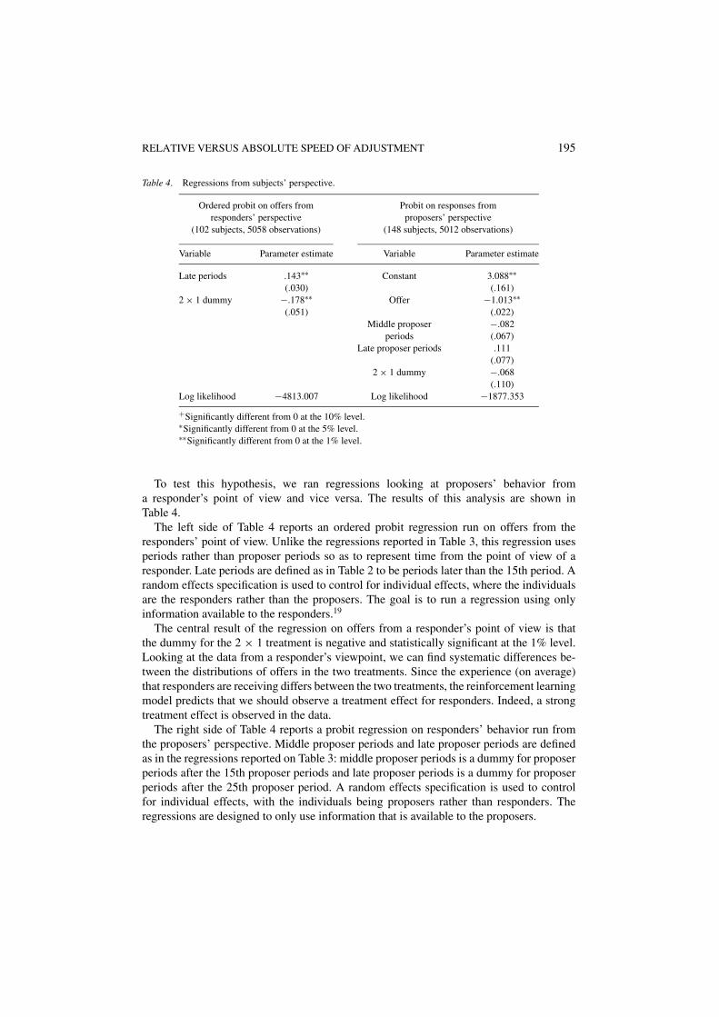
Table 4. Regressions from subjects’ perspective.

Ordered probit on offers from Probit on responses fromresponders’ perspective proposers’ perspective

(102 subjects, 5058 observations) (148 subjects, 5012 observations)

Variable Parameter estimate Variable Parameter estimate

Late periods .143∗∗ Constant 3.088∗∗(.030) (.161)

2 × 1 dummy −.178∗∗ Offer −1.013∗∗(.051) (.022)

Middle proposer −.082periods (.067)

Late proposer periods .111(.077)

2 × 1 dummy −.068(.110)

Log likelihood −4813.007 Log likelihood −1877.353


To test this hypothesis, we ran regressions looking at proposers’ behavior froma responder’s point of view and vice versa. The results of this analysis are shown inTable 4.

The left side of Table 4 reports an ordered probit regression run on offers from theresponders’ point of view. Unlike the regressions reported in Table 3, this regression usesperiods rather than proposer periods so as to represent time from the point of view of aresponder. Late periods are defined as in Table 2 to be periods later than the 15th period. Arandom effects specification is used to control for individual effects, where the individualsare the responders rather than the proposers. The goal is to run a regression using onlyinformation available to the responders.19

The central result of the regression on offers from a responder’s point of view is thatthe dummy for the 2 × 1 treatment is negative and statistically significant at the 1% level.Looking at the data from a responder’s viewpoint, we can find systematic differences be-tween the distributions of offers in the two treatments. Since the experience (on average)that responders are receiving differs between the two treatments, the reinforcement learningmodel predicts that we should observe a treatment effect for responders. Indeed, a strongtreatment effect is observed in the data.

The right side of Table 4 reports a probit regression on responders’ behavior run fromthe proposers’ perspective. Middle proposer periods and late proposer periods are definedas in the regressions reported on Table 3: middle proposer periods is a dummy for proposerperiods after the 15th proposer periods and late proposer periods is a dummy for proposerperiods after the 25th proposer period. A random effects specification is used to controlfor individual effects, with the individuals being proposers rather than responders. Theregressions are designed to only use information that is available to the proposers.

196 COOPER ET AL.

The critical variable in interpreting this regression is once again the 2 × 1 treatmentdummy. While the coefficient on this variable has the correct sign, it is not statistically sig-nificant at any standard level. This result implies that the experience proposers are receivingin the two treatments does not differ significantly. As such, the reinforcement learning modeldoes not predict that we will find a treatment effect, and indeed we don’t.20

To summarize, the presence or absence of treatment effects for the two roles is consistentwith the reinforcement learning model once we account for the presence or absence ofobservable differences in the experience subjects receive in the two treatments.

On a broad level, the experimental results are consistent with the reinforcement learningmodel. The reinforcement learning model predicts that responders adjust more slowly thanproposers in the ultimatum game because their incentives to change their behavior aremuch lower. Because the relative speed of adjustment is slower for responders than forproposers, proposers stop making low offers before responders learn to accept them. The2 × 1 treatment is designed to manipulate the relative speeds of adjustment so that responderswill both receive more low offers and receive them farther into the experiment. Havinggiven the responders more relevant experience, we expect to see more adjustment towardsaccepting low offers. This is exactly what is observed. Rejection rates are lower in the 2 ×1 treatment than in the 1 × 1 treatment.

5. Conclusions

The experiment described in this paper is designed to elicit a subtle yet important effect.By successfully detecting learning by the responders, we show that a critical empiricalprediction of reinforcement learning models is fulfilled. The data are consistent with theresponders learning in exactly the same manner that the proposers learn. The famouslyanomalous behavior of responders in the ultimatum game need not depend on respondershaving unchanging preferences for fairness, but instead can be explained by the relativelyslow speed of responders’ learning as compared with proposers’ learning.

Our point is not that the magnitude of learning by responders in the ultimatum game isespecially large. The learning theories predict that responders will learn only slowly, and thepositive evidence of a small effect collected here is consistent both with these predictionsand with previous studies in which no responder learning was detected. It is because learningby responders is so difficult to detect that the responder learning detected here says as muchabout the learning models as does their success at predicting behavior in games in whichlearning is much more evident. Successful models should allow us to predict non-obviouseffects that haven’t yet been observed as well as the obvious ones we already know about.If learning models were only successful at predicting behavior in games in which rapidlearning is evident, we could not be as confident that the models were capturing the causeof the learning behavior, and not just its gross effects. The successful observation of thepredicted responder learning in the 2 × 1 condition allows us to have greater confidence inthe explanatory as well as the predictive power of learning theories.

Our results do not imply that theories of fairness have no role to play in understandingbehavior in the ultimatum game and related games. The learning models do a good jobof explaining how behavior evolves given a starting configuration of strategies, but do


not explain how this initial state arises. Theories of fairness have a natural role to playin explaining the initial state of play. Moreover, work on related games by Cooper andStockman (2000) has shown that models that combine fairness and learning do a better jobof capturing the major features of the data than models that use just fairness or just learning.We have done similar exercises with the data set reported in this paper (Cooper et al., 1999),and also find that a hybrid model combining fairness and learning outperforms a puremodel. Thus, while our results indicate that learning by responders must be accounted forin understanding the ultimatum games, explanations of responder behavior in the ultimatumgame also leave a role for theories incorporating preferences concerning fairness.

We are not the first experimenters to study learning by responders, but we believe our workrepresents a significant step forward in understanding learning by responders. In particular,we have found unambiguous evidence of learning by responders. Most experiments thatallow players to gain experience reveal changes over time in the offers, but have been unableto detect changes in the acceptance/rejection behavior of responders. (See e.g. Roth et al.,1991; Slonim and Roth, 1998; Duffy and Feltovich, 1999).

The notable exception to this statement is List and Cherry (2000).21 That paper repli-cates the earlier work of Slonim and Roth (1998) while adding an element of proposerentitlement.22 In the low stakes treatment, no changes in responders’ behavior are observedover the ten periods of the experiment. In the high stakes treatment, there is a statisticallydetectable decrease in the rejection rates by responders over the final three periods. List andCherry do not attribute this change to any specific cause, but do note that it is consistentwith the learning model of Roth and Erev.

Our work both complements the work of List and Cherry and adds to it substantially.List and Cherry note that their two differing treatments generate different distributionsof offers, and conjecture that this difference in distributions drives the differing behaviorby responders. Our results largely confirm this conjecture. Our work expands the workof List and Cherry in three specific ways, listed in order of increasing importance. (1)Because their purpose was not to study responder learning, List and Cherry’s experimentaldesign includes potential confounds that could explain their results. Our experiments arecompletely standard ultimatum games from the subjects’ points of view with no potentialconfound. (2) The effect found by List and Cherry is an endgame effect, and is consistentwith subjects abandoning a reputation for toughness. This suggests that the changes inresponders’ behavior they found may not necessarily be due to learning in the sense wetypically think of it. The effects we find in our data are in no sense endgame effects. (3)We clearly demonstrate that changes in responders’ behavior are driven by the stream ofoffers they are receiving. In other words, we aren’t just seeing a decline in errors for someunknown reason, we aren’t just seeing an endgame effect, but rather we are seeing truelearning in which subjects are responding to their experiences by changing their behavior.

On a broader level, it bears repeating that while showing that responders learn is animportant result, our purpose is more than this. The theoretical argument that this paperexplores depends on differences in relative speeds of learning—the prediction that play inthe ultimatum game need not converge to the subgame perfect equilibrium follows from theobservation that while responders learn in the same fashion as proposers, they learn moreslowly than proposers. This implies manipulating the relative speeds of learning can alter thebehavior that we observe. Our goal, which we have achieved, was to verify this prediction.

198 COOPER ET AL.

Appendix A

This appendix contains technical material describing the reinforcement learning model andexplaining how simulations of this model were implemented.

A.1. Description of the reinforcement learning model

The model for each individual is specified as follows. At time t = 1 (before any experiencehas been acquired) each player n has an initial propensity to play his kth pure strategy,given by some number qnk(1). If player n plays his kth pure strategy at time t and receives apayoff of x , then the propensity to play strategy k is updated by setting qnk(t + 1) = φqnk(t)+ x , while for all other pure strategies j , qnj (t + 1) = φqnj (t), where 0 < φ < 1 is a“forgetting” parameter that regulates how slowly past experience decays. The probabilitypnk(t) that player n plays his kth pure strategy at time t is pnk(t) = qnk(t)/�qnj (t), wherethe sum is over all of player n’s pure strategies j . The model thus has two parameters, φ,and the sum over all pure strategies j of a player’s initial propensities, S = φqnj (1). Thislatter parameter, which is taken to be the same for all players, is called the “strength” of theinitial propensities, and influences the early speed of learning.

Thus this model predicts that strategies that have been played and have met with successtend over time to be played with greater frequency than those that have met with less success;i.e. these dynamics obey the “law of effect.” Also, the learning curve will be steeper in earlyperiods and flatter later (because �qnj (t) is an increasing function of t , so a payoff of xfrom playing pure strategy k at time t has a bigger effect on pnk(t) when t is small thanwhen t is large, i.e. the derivative of pnk(t) with respect to a payoff of x is a decreasingfunction of t).

A.2. Implementation of the reinforcement learning model to predict the outcomeof the experiment

In using the reinforcement learning model to predict the outcome of the current experiment,we begin by specifying a strategy set for each player. For the proposers, the strategy setequals the set of available offers, {1, 2, . . . ,10}. For responders, we follow Roth and Erev(p. 177) in limiting the set of available strategies to be cutoff strategies. A cutoff strategyspecifies the lowest offer that a player would be willing to accept. For example, an individualwith a cutoff of 4 will accept any offer greater than or equal to 4, and will reject lower offers.The set of available cutoffs corresponds to the set of available offers, {1, 2,. . .,10}.23

Having limited responders to cutoff strategies, the learning model can be applied to theultimatum game as a normal form game in which each of the two players chooses a numberbetween 1 and 10 simultaneously. Let O be the offer selected and C be the cutoff selected.The following equations give the proposer’s payoff, πP, and the responder’s payoff, πR.

πP(O, C) = 10 − O if O ≥ C

= 0 otherwise (1a)


πR(O, C) = O if O ≥ C

= 0 otherwise (1b)

To predict differences between the 1 × 1 treatment and the 2 × 1 treatment, we ran 10,000simulations of each treatment. The simulations of the 1 × 1 treatment use two populationsof ten individuals (represented by the learning model), ten proposers and ten responders,with all individuals playing in each period. The simulations of the 2 × 1 treatment usethree populations of ten players, two groups of ten proposers and ten responders. As inthe actual experiments, the responders play each period while the two groups of proposersalternate periods. The proposers and responders playing in any particular period are ran-domly matched. All of the simulations last for 50 periods, the modal number of periodsfor the actual experiments. This allows us only 25 periods to compare proposers’ behaviorbetween the two treatments.

Our goal in running these simulations was to generate qualitative predictions for the effectof the 2 × 1 treatment, not to find the best fit for some particular data set. Therefore, ourapproach is to choose a plausible set of parameters, determine the predicted treatment effects,and then see how robust these predictions are to changes in the parameters. For simplicity,we use the same initial probabilities over offers and cutoffs for all of the simulations andonly vary the strength of initial propensities and the forgetting parameter. For simplicity,all individuals are assumed to have identical initial propensities.24 The initial propensitiesfor proposers put weights of 33.3% on an offer of 5, 33.3% on an offer of 4, 16.7% on anoffer of 3 and 16.7% on an offer of 2. The initial propensities for responders put weights of20% on a cutoff of 5, 40% on a cutoff of 4, 20% on a cutoff of 3, and 20% on a cutoff of 0.The implied initial reject rates are 0% for an offer of 5, 20% for an offer of 4, 60% for anoffer of 3, and 80% for an offer of 2. Initially, an offer of 5 maximizes expected payoffs bya narrow margin. These initial propensities are in the ballpark of what is typically seen inultimatum game experiments. In the baseline simulations, the initial strength of propensitieswas set equal to 10 for all individuals and the forgetting parameter was set equal to 1 for allindividuals. We then vary these values to evaluate the sensitivity of the model’s predictionsto the parameters.

Appendix B

This appendix contains technical material on the regressions described in Sections 4.1 and4.3.

B.1. Regressions on responder data

All of our econometric analysis of responders’ data uses probit regressions. The dependentvariable is always the responder’s choice, with an acceptance coded as a 0 and a rejectioncoded as a 1. Thus, positive parameters correspond to a higher probability of rejectionand negative parameters correspond to higher probability of acceptance. Statistical tests of

200 COOPER ET AL.

significance for individual parameter estimates are always two-tailed z-tests, and tests ofjoint significance are always log-likelihood ratio tests.

Many of our regressions include lagged variables. Due to this, the first period of data isdeleted from our data set. Other than this we have used all observations from all responders.

Casual investigation of the data indicates that there are strong individual effects in theresponder data. A random effects specification, allowing for correlation between observa-tions from the same individual, is used to correct for these individual effects. The regressionresults strongly support the use of a random effects specification since the random effectsterm is always significant at the 1% level. We do not report the estimate of the randomeffects term in our tables, since it has no economic relevance.25

Several of our regressions include measures of past behavior by proposers. We use threevariables to measure proposers’ past behavior: the proportion of previous offers greaterthan or equal to 5 (high offers), the proportion of previous offers less than or equal to 3(low offers), and the lagged offer from the preceding period. All three of these measures arecalculated using the individual responder’s past history—no information that a subject couldnot have observed is used. The first two variables allow us to control for the distributionof past offers without imposing linearity while the third controls for the possibility thatthe most recent experience gets extra weight. While these three measures of proposers’behavior are closely related to each other, they are far from being perfectly correlated.26

Since we are interested in learning effects, our analysis includes controls for changes intime. We use a non-linear specification for time, with the variable “Late Periods” being adummy for observations after the 15th period. We tested a variety of alternative specificationsfor time, including linear specifications and non-linear specification with more intervals,and found that this one best fits the data. The choice of specifications for time does notaffect any of our main conclusions.27

B.2. Regressions on proposer data

Our econometric analysis of proposer data uses ordered probit regressions. Our use of thisnon-linear specification is driven by the discreteness of proposer data. Unlike many ultima-tum game experiments in which subjects are choosing (approximately) over a continuum,proposers in our experiments only have a small number of possible strategies. We can there-fore think of the observable choices as categories capturing subjects’ underlying choicesover the continuum of possible offers.

Offers are classified into three categories: offers less than or equal to 3, offers of 4, andoffers of 5 or greater. The first period of data is deleted to allow for the use of laggedvariables. Since there are strong individual effects in the proposer data, we use a randomeffects specification. The breakpoints between categories and the random effects term arenot reported in our tables. While these items are always statistically significant, they lackany economic significance. The ordered probit regressions do not contain a constant sincethis would be colinear with the breakpoints.28

All regressions on proposer data measure time from the perspective of the proposer.Thus, the tenth period of a 2 × 1 session is considered equivalent to the fifth period of a1 × 1 session, since in both cases the proposer is playing for the fifth time. We refer to the


“proposer period” to make it clear that we are referring to the number of times a proposer hasplayed. We use proposer periods to avoid comparing apples with oranges. It isn’t surprisingthat a proposer playing for the tenth time is different from one playing for the fifth time,given the strong learning dynamic in the data. Instead, we are trying to find differencesbetween subjects who have played the same number of times in different treatments.

As with responders, we use a non-linear specification for time with proposers. We sub-divide proposer periods into three classes: proposer periods 1–15, proposer periods 16–25,and proposer periods 26–60. We refer to these as early, middle, and late proposer periodsrespectively. The break following 15 proposer periods is used to parallel our analysis ofresponders’ data. The break following 25 proposer periods isolates proposer periods thatonly contain data from 1 × 1 sessions. This guarantees that differences we identify betweenthe treatments aren’t due solely to the fact that there are twice as many proposer periods inthe 1 × 1 sessions.29 The regressions include a dummy for proposer periods greater than15 (“middle proposer periods”) and a dummy for proposer periods greater than 25 (“lateproposer periods”). Thus, the parameter labeled “late proposer periods” reflects the differ-ence between offers in the middle proposer periods and offers in the late proposer periods,not between offers in the early proposer periods and offers in the late proposer periods.

Model 3 on Table 3 modifies Model 1 by adding three measures of responders’ behavior.In choosing the variables to be included, many obvious measures of responders’ behaviorcould not be used because of concerns with endogeneity and sample censoring.30 We employthe rejection rates for offers of 5, offers of 4, and for offers of 3. These three rejection ratesare calculated at the session level. For example, the rejection rate for offers of 4 is basedon the responses to all previous offers of 4 by any proposer in the same session as thesubject whose behavior we are trying to predict. While the session rejection rate differsfrom the rejection rate observed by any one individual, session rejection rates should behighly correlated with the responses observed by individual proposers. Therefore we believethat the session rejection rates are good proxies for the responder behavior observed by anindividual subject.31

Appendix C: Instructions

The purpose of this session is to study how people make decisions in a particular situation.During this session you are going to participate in several rounds of negotiations. In each

round the group of people in the room is divided into pairs. Each pair will bargain on howto divide $10.00.

How do you bargain on the division?

One of you, the PROPOSER, will propose a division of the money. The person who re-ceives the offer, the RESPONDER, can either accept or reject it. In either case the roundENDS immediately after the response to the offer is made. If the RESPONDER accepts theproposed division, then the money is divided accordingly. If the RESPONDER rejects theproposed division the round ends in disagreement and EACH one of you receives nothing.

202 COOPER ET AL.

PROPOSER RESPONDER$9.00 $1.00$8.00 $2.00$7.00 $3.00$6.00 $4.00$5.00 $5.00$4.00 $6.00$3.00 $7.00$2.00 $8.00$1.00 $9.00$0.00 $10.00

In this session, the PROPOSER can not demand more than $9.00 for him/herself outof the $10.00. Also, the amounts must be multiples of $1.00. Hence, the PROPOSER canpropose only one of the following 10 divisions:

YOU WILL HAVE THE SAME ROLE, PROPOSER OR RESPONDER, IN ALLROUNDS. Your role will be determined randomly.

How do you get paid for your participation?

For completing the session you will receive $5.00. During the session you will participatein a series of rounds described above. At the end of the session, one of the rounds will bechosen at random, and you will be paid in cash what you earned in that round, in additionto the $5.00.

Who are the bargainers?

In each round the computer will randomly assign you to another person with whom youwill bargain. You will never bargain with the same player twice in a row. Since you areinteracting using the computer terminal, you will not know your co-bargainer’s identity,nor will they know yours. These identities will not be revealed even after the session iscompleted.

How to use the computer terminal

The whole session in managed by a computer program. All exchanges (offers and responses)are done through the terminal in front of you. You key in offers/responses using the keyboardand watch for responses and other information by observing the screen.

The PROPOSER makes an offer by filling in his/her proposed share of the $10.00in the following statement on the screen: “I propose to get $X.00 out of the $10.00.”The PROPOSER should type in one number to replace the X on the screen. After doing sothe computer will display the proposal back and will ask for verification. At that point, thePROPOSER can revise his/her proposal if so desired.


A confirmed proposal will be sent to the RESPONDER who will be asked to accept orreject it, by typing A for accept and R for reject. After doing so the computer will ask forverification. At that point, the RESPONDER can change his/her decision if so desired.

At the bottom of the screen you will find a “History of Past Play” window. This windowwill display the outcomes of previous rounds you have played.

Note that a new round will start only after all games played in the previous round arefinished. Since there are many players in this session, expect delays between rounds. Pleasebe patient.

During the session you may not communicate with other participants expect through thecomputer terminals. If you have any questions during the session, raise your hand and amonitor will come speak to you.

Instructions will now be read out loud, and any questions will be answered.

Acknowledgments

We would like to thank John Ham, Glenn Harrison, Hidehiko Ichimura, John List, andBob Slonim for their helpful comments. As per usual, the authors of this paper are solelyresponsible for any errors it may contain.

Notes

1. It was initially studied by Guth et al. (1982); see Roth (1995) for a survey of related work.2. The term reinforcement learning is here meant broadly, and certainly includes the replicator dynamics used

by Gale et al. (1995) to derive a similar explanation to the one discussed here.3. In addition to the papers cited earlier, see also Bornstein et al., 1994, 1996; Cooper et al., 1997; Erev, 1998;

Erev and Rapoport, 1998; Feltovich, 2000, Mookherjee and Sopher, 1994, 1997; Nagel and Tang, 1998;Rapoport et al., 1997, 1998; Roth et al., 2000; Sarin and Vahid, 2000; Tang, 1995; Van Huyck et al. 1994.

4. There also exists a literature on the evolutionary foundations for such preferences. See Samuelson, 2001, fora concise summary of this literature.

5. According to this view, the learning observed on the part of proposers is simply ordinary Bayesian learningabout the parameters of responders’ utility functions.

6. The reinforcement learning model also predicts a second order effect on proposer behavior, that reinforcesthe difference between the two conditions. The prediction is that, in the 2 × 1 condition, since the (lessexperienced) proposers will be encountering responders who more quickly learn to accept low offers than inthe 1 × 1 condition, the proposers in the 2 × 1 condition will learn not to make low offers more slowly thanequally experienced proposers in the 1 × 1 condition.

7. Average earnings were roughly $9.00 for a two-hour session. Subject payments were made in cash immediatelyfollowing the session.

8. A comparison of some of the newer learning models can be found in Erev et al. (2002).9. See Erev and Roth (1998) for a discussion of variations on the basic reinforcement model. For an alternative

approach to reinforcement learning that does not obey the Power Law of Practice, see Bush and Mosteller(1955) as well as Cross (1983).

10. Guth et al. (2001) find evidence that some individuals in ultimatum game experiments do not use cutoffstrategies. However, given that 91% of their subjects do use cutoff strategies, we feel that the use of cutoffstrategies is a defensible simplification. The model’s qualitative predictions do not depend on this assumption.

11. Cooper et al. (1999) contains such a fitting exercise.12. Specifically we set the initial strength equal to 10, and set the forgetting parameter equal to 1. Setting the rate

of forgetting equal to 1 is equivalent to not including any forgetting in the model.

204 COOPER ET AL.

13. We consider all possible combinations of initial strength = 2.5, 10, and 40 and the forgetting parameter =.8 and 1.0. This gives us six sets of simulations including the baseline simulations. The choice of only sixparameter combinations is made to keep the graphs relatively readable. Adding more parameter values wouldnot affect our predictions. Likewise, we use the same initial probabilities for the players’ strategies in all ofthe simulations to simplify matters, but our predictions would not change if we used a variety of differinginitial probabilities.

14. Specifically, the strength of initial propensities is equal to 2.5 and the forgetting parameter is equal to .8.15. All of our econometric analysis of responders’ behavior uses the offer as an explanatory variable. To the extent

that offers are endogenous, this could raise problems with our analysis. We are analyzing data at the individuallevel. There is negative correlation between the likelihood of receiving a low offer and the likelihood thatresponders in a particular session will reject such an offer. There must be positive correlation between thelikelihood that a particular individual rejects a low offer and the likelihood that a responder randomly selectedfrom his session rejects a low offer. Implicitly, we are assuming that our sessions are large enough that theproduct of these two correlations is small.

16. Beyond the main treatment variable, one unusual feature of our experiments is the large number of repetitions.One could argue that, compared with single-shot experiments, this might bias subjects towards using simpleadaptive algorithms rather than trying to reason through the game. If this were true, we would expect first playbehavior to be altered. However, comparing the first play behavior in our experiment with that observed inother ultimatum game experiments, we see no evidence to support this hypothesis. In particular, we gatheredfirst period data from Guth et al.’s inexperienced sessions (1982), Forsythe et al’s. (1994) ten dollar ultimatumgames, and Roth et al.’s (1991) ten dollar ultimatum games from Pittsburgh. The first two experiments aresingle-shot, with Forsythe et al. being run in the U.S. for the same stakes we used. The Roth et al. sessionsrepeated the game ten times, but used the same population and the same stakes as the current experiments.Comparing first play offers across these four experiments, our subjects are neither the most generous nor theleast. To see this, we can break first offers into three categories: 50% of the pie or more, 40–49% of the pie,and less than or equal to 39% of the pie. For our experiment, the proportions of proposers in these categoriesare .439, .338, and .223 respectively. The respective proportions for the other experiments are .238, .167, and.595 for Guth et al., .750, .125, and .125 for Forsythe et al., and .593, .259, and .148 for Roth et al. Proposersfrom the Forsythe et al. experiments are the most generous while those from the Guth et al. experimentsare the least generous. Looking at rejection rates, our subjects again look unexceptional. Breaking down theoffers into the same three categories as above, we get rejection rates of .000, .243, and .355 for the currentexperiments. The respective numbers for the other experiments are .071, .143, and .280 for Guth et al., .000,.167, and .000 for Forsythe et al., and .188, .167, and .500 for Roth et al. These numbers should be taken witha grain of salt, since the number of observations in any category is relatively small. However, no clear rankingemerges among the four experiments for first period rejection rates.

17. We report marginal effects calculated at the average values of the independent variables. Given the non-linearityof the probit model, the predicted effect on rejection rates will differ for any particular offer.

18. Another possible explanation rests on the statistics being used. As indicated by the simulations, the treatmenteffect can be quite small while the individual effects in the data are substantial. Our ability to pick up treatmenteffects in the data depends on our ability to separate individual effects from systematic treatment effects. Themore observations we have for each individual in our sample, the easier it becomes to disentangle individualand treatment effects. The experimental design gives us only 25 proposer periods in which we can make adirect comparison between the two treatments for proposers, as opposed to 50 periods for the responders.For all practical purposes, we are trying to detect a subtle treatment effect for proposers with a substantiallysmaller data set than the data set for responders. Not surprisingly, it is harder to detect a treatment effect witha smaller data set.

19. Unlike the regressions in Tables 2 and 3, neither regression in Table 4 includes an interaction effect be-tween the treatment dummy and the time dummies. This simplified specification is used to maximize ourchance of detecting a statistically significant treatment effect. Including interaction terms would not affect ourconclusions.

20. It isn’t surprising that we find a difference in responder’s behavior between the two treatments in Table 2 butnot in Table 4. The regressions in Table 2 use information that is not available to proposers, and therefore isnot incorporated into the regressions in Table 4.


21. Harrison and McCabe (1996) also report an experiment on an ultimatum-like game where they find decliningcutoffs for responders. Reflecting the primary purpose of their work, studying the effects of different varietiesof feedback on subject behavior, the methodologies and the ultimatum game used in this experiment departsignificantly from those typically used in ultimatum game experiments. Indeed, several of their sessionsconverge toward the perfect equilibrium, certainly not a standard ultimatum game result. The two sessionsclosest to standard ultimatum game experiments both in methods and results are their two control sessionsU1 and U1′ which show similar declines in the responders’ cutoffs. This is interesting, because subjects arereceiving no feedback whatsoever in U1 while they receive standard feedback on their opponent’s choice inU′

1. This odd result, albeit based on a small sample, indicates that we need to be very careful about labelingchanges in responder behavior as learning. Most models of learning, including all models of reinforcementlearning, have players modifying their actions in response to feedback about previous outcomes. As such,establishing a link between the feedback and responders’ choices is a necessary condition for a meaningfulclaim of learning. Changes by themselves may indicate nothing more than reduced subject confusion or greaterintrospection due to having more time to think.

22. Proposers were assigned to the high or low stakes payoff treatment based on their performance on a quiz.Responders were told that proposers had “earned an amount of money (the pie being bargained over) byparticipating in a previous session.”

23. For symmetry with proposers (who cannot offer 0), we don’t allow for the possibility that an offer of 10 willbe rejected. Given the rarity of such offers, this is not an important restriction to the model.

24. Consistent with the use of a random effects specification in the econometric analysis of our data, we couldhave assumed that initial propensities are drawn from a random distribution. If we were trying to generatea best fit to the experimental data, such a specification could potentially play a valuable role. However,for our limited purposes this just adds extra complexity to the simulations without materially affecting thepredictions.

25. More specifically, a random effects specification estimates the correlation between observations from thesame individual (rho). This acts as an additional parameter in the maximum likelihood estimation. Rejectingthe null hypothesis that this parameter equals zero tells us that observations from the same individual are notstatistically independent. For example, for the key regression in Table 2, Model 2, the estimated value of rhois .618 with a standard error of .013. This indicates a strong rejection of the null hypothesis of independence.

26. The correlation between the proportion of high offers and the proportion of low offers is −.550. The correlationbetween the proportion of high offers and the offer from the preceding period is .375. The correlation betweenthe proportion of low offers and the offer from the preceding period is −.402.

27. To the extent that alternative specifications for time affect our results, we find that the treatment effect forresponders widens significantly over time with some specifications. Since this result is not robust to the choiceof specifications, we put little weight on it. We have also explored specifications in which the measures ofpast proposer behavior are interacted with the dummy for late periods. We do not find that these specificationssignificantly improve our ability to fit the data.

28. We limited the number of categories for offers to avoid convergence problems in the estimation. Given thatover 90% of offers are in the 3–5 range, we lost little by eliminating separate categories for the extreme offers.As a robustness check, we have also run linear regressions with a random effect specification and orderedprobits using all possible offers as categories and the method suggested by Moulton (1986) to correct thestandard errors for clustering. In both cases, the qualitative results are identical to those reported in Table 3.This indicates that neither the use of an ordered probit specification nor the limited number of categories aredriving our results.

29. Without adding in this extra time class, we find significantly lower offers in the 2 × 1 sessions. This is afalse positive, reflecting the fact that offers continue to rise beyond the 25th proposer period, the last proposerperiod in the 2 × 1 sessions.

30. For a detailed discussion of the limitations we faced in constructing measures of responders’ behavior, seethe working version of this paper (Cooper et al., 1999).

31. We do not use the session rejection rates as instrumental variables per se. For our purposes there is little tobe gained by using instrumental variables, and the technical problems raised by trying to use instrumentalvariables with an ordered probit regression would be substantial.

206 COOPER ET AL.

References

Blackburn, J.M. (1936). “Acquisition of Skill: An Analysis of Learning Curves.” IHRB Report No. 73.Bolton, G. (1991). “A Comparative Model of Bargaining: Theory and Evidence.” American Economic Review.

81, 1096–1136.Bolton, G.E. and Ockenfels, A. (1999). “ERC: A Theory of Equity, Reciprocity and Competition.” American

Economic Review, forthcoming.Bornstein, G., Erev, I., and Goren, H. (1994). Learning processes and reciprocity in intergroup conflicts. Journal

of Conflict Resolution. 38, 690–707.Bornstein, G., Winter, E., and Goren, H. (1996). “Experimental Study of Repeated Team Games.” European

Journal of Political Economy Volume 12, Issue 4, 17-December-1996.Cooper, D.J., Garvin, S., and Kagel, J.H. (1997). “Adaptive Learning versus Equilibrium Refinements in an Entry

Limit Pricing Game.” Economic Journal. 107, 553–575.Cooper, D.J., Feltovich, N., Roth, A.E., and Zwick, R. (1999). “Relative versus Absolute Speed of Adjustment in

Strategic Environments: Responder Behavior in Ultimatum Games.” Working Paper.Cooper, D.J. and Stockman, C.K. (2002). “Fairness and Learning in a Step-Level Public Goods Game.” Games

and Economic Behavior. 41, 26–45.Duffy, J. and Feltovich, N. (1999). “Does Observation of Others Affect Learning in Strategic Environments? An

Experimental Study.” International Journal of Game Theory. 28, 131–152.Erev, I. (1998). “Signal Detection by Human Observers: A Cutoff Reinforcement Learning Model of Categorization

Decisions Under Uncertainty. Psychological Review. 105, 280–298.Erev, I. and Rapoport, A. (1998). “Magic, Reinforcement Learning and Coordination in a Market Entry Game.”

Games and Economic Behavior. 23, 146–175.Erev, I. and Roth, A.E. (1998). “Predicting how people play games: Reinforcement learning in experimental games

with unique, mixed strategy equilibria,” American Economic Review. 88(4), 848–881.Erev, I., Roth, A.E., Slonim, R.L., and Barron, G. “Combining a Theoretical Prediction with Experimental Evi-

dence.” Revised 2002.Fehr, E. and Schmidt, K.M. (1999). “A Theory of Fairness, Competition, and Cooperation.” Quarterly Journal of

Economics. 114, 817–868.Feltovich, N. (2000). “Reinforcement-Based vs. Beliefs-Based Learning Models in Experimental Asymmetric-

Information Games.” Econometrica. 68, 605–641.Forsythe, R., Horowitz, J., Savin, N.E., and Sefton, M. (1994). “Fairness in Simple Bargaining Experiments.”

Games and Economic Behavior. 6, 347–369.Gale, J., Binmore, K., and Samuelson, L. (1995). “Learning to be Imperfect: The Ultimatum Game.” Games and

Economic Behavior 8, 56–90.Guth, W., Schmittberger, R., and Schwarz, B. (1982). “An Experimental Analysis of Ultimatum Bargaining.”

Journal of Economic Behavior and Organization. 3, 367–388.Harrison, G. and McCabe, K. (1996). “Expectations and Fairness in a Simple Bargaining Experiment.” Interna-

tional Journal of Game Theory. 25, 303–327.List, J. and Cherry, T. (2000). “Learning to Accept in Ultimatum Games: Evidence from an Experimental Design

the Generates Low Offers.” Experimental Economics. 3, 11–30.Mookherjee, D. and Sopher, B. (1994). “Learning Behavior in an Experimental Matching Pennies Games.” Games

and Economic Behavior. 7, 62–91.Mookherji, D. and Sopher, B. (1997). “Learning and Decision Costs in Experimental Constant Sum Games.”

Games and Economic Behavior. 19(1), 97–132.Moulton, B. (1986). “Random Group Effects and the Prevision of Regression Estimates.” Journal of Econometrics.

32, 385–397.Nagel, R. and Tang, F.F. (1998). “Experimental Results on the Centipede Game in Normal Form: An Investigation

on Learning.” Journal of Mathematical Psychology. 42, 356–384.Ochs, J. and Roth, A.E. (1989). “An Experimental Study of Sequential Bargaining.” American Economic Review.

79, 355–384.Rabin, M. (1993). “Incorporating Fairness into Game Theory and Economics.” American Economic Review. 83,

1281–1302.


Rapoport, A., Erev, I., Abraham, E.V., and Olson, D.E. (1997). “Randomization and Adaptive Learning in aSimplified Poker Game.” Organizational Behavior and Human Decision Processes. 69, 31–49.

Rapoport, A., Seale, D., Erev, I., and Sundali, J.A. (1998). “Coordination Success in Market Entry Games: Testsof Equilibrium and Adaptive Learning Models.” Management Science. 44, 119–141.

Roth, A.E. (1995). “Bargaining Experiments.” Handbook of Experimental Economics, J. Kagel and A.E. Roth(eds.). Princeton University Press, pp. 253–348.

Roth, A.E. and Erev, I. (1995). “Learning in Extensive-Form Games: Experimental Data and Simple DynamicModels in the Intermediate Term.” Games and Economic Behavior, Special Issue: Nobel Symposium. 8, 164–212.

Roth, A.E., Prasnikar, V., Okuno-Fujiwara, M., and Zamir, S. (1991). “Bargaining and Market Behavior inJerusalem, Ljubljana, Pittsburgh, and Tokyo: An Experimental Study.” American Economic Review. 81, 1068–1095.

Samuelson, L. (2001). “Introduction to the Evolution of Preferences.” Journal of Economic Theory. 97, 225–230.Sarin, R. and Vahid, F. (2001). “Predicting How People Play Games: A Simple Dynamic Model of Choice.” Games

and Economic Behavior. 34, 104–122.Slonim, R. and Roth, A.E. (1998). “Learning in High Stakes Ultimatum Games: An Experiment in the Slovak

Republic.” Econometrica. 66(3), 569–596.Tang, F.-F. (1995). “Anticipatory Learning in Two-Person Games: An Experimental Study.” Dissertation, Univer-

sity of Bonn.Thorndike, E.L. (1898). Animal Intelligence: An Experimental Study of the Associative Processes in Animals.

Psychological Monographs, 2.Van Huyck, J.B., Cook, J.P., and Battalio, R.C. (1994). “Selection Dynamics, Asymptotic Stability, and Adaptive

Behavior.” Journal of Political Economy. 102, 975–1005.

relative versus absolute speed of adjustment in...

Documents