relationships between air quality, health and...
TRANSCRIPT

Relationships between Air Quality,Health and Economy
C. Arden Pope III, PhDMary Lou Fulton Professor of Economics
Brigham Young University
International Sustainable Development SchoolTraining for Sustainability
2017: Air QualityOctober 30-November 3, 2017

What do we breathe?
Pure Air--nitrogen (78%), oxygen (21%), argon . . .
+Air pollutants, including:➢Various gaseous pollutants (SO2, NO2, CO, O3 . . . )
➢Particulate matter:Course particles (> 2.5 µm in diameter)
PM2.5—Fine particles (< 2.5 µm in diameter)
➢Other air toxics

How small are fine particles?
Human Hair
(60 mm diameter)
PM10
(10 mm)
PM2.5
(2.5 mm)

Magnified ambient particles (www.nasa.gov/vision/earth/environment)

Beijing, ChinaIndia--Lucknow, Chandigarh, Jaipur
Salt Lake City, UtahIndia--Agra (Taj Mahal)Medellin, Colombia

1st Controversy:
Was London smog romantic or deadly?
Peter Ellenshaw paintings from Mary Poppins

Claude Monet,
Houses of Parliament,
London,1903

Old King Coal and the Fog Demon brings asthma, pneumonia, pleurisy and bronchitis to London.
Cartoon from British humor magazine Punch, 1880.
Image: Public Domain Review

Romantic vs. deadly controversy largely resolved with three well-documented air pollution episodes.
Dec. 5-9, 1952: London--1000’s of excess deaths
Dec. 1-5, 1930: Meuse Valley, Belgium60 deaths (10x expected)
Oct. 27-31, 1948: Donora, PA20 deaths, ½ the town’s population fell ill
Respiratory and cardiovascular disease and death

London Fog Episode, Dec. 1952
From: Brimblecombe P. The Big Smoke, Methuen 1987
David Bates, MDSt. BartholomewMcGill U, UBC

Killer Smog (and related research)
Public Policy Results1955-1967: Air pollution control
acts
1967, 1970: Clean Air Act, EPAMajor Amendments, National
Environmental Policy Act
1977 & 1990: Major Amendments
to Clean Air Act
1980’s: Elimination of
extreme “Killer Smog” episodes & Improved air quality
1930: Meuse Valley, Belgium
1948: Donora, PA
1952: London, England
National Ambient Air Quality Standards

1st Controversy:
Were extreme smog episodes romantic or deadly?
Answer: Deadly
2nd Controversy:
Can short-term exposure to moderate levels of pollution hurt us?

Utah Valley, 1980s
• Winter inversions trap local pollution
• Natural test chamber
• Local Steel mill contributed ~50% PM2.5
• Shut down July 1986-August 1987• Natural Experiment

Geneva Steel, Utah Valley, 1989 (PM10 = 150 mg/m3)

Air pollution workshop participants in front of Geneva Steel, March 19-20, 1992
Joel SchwartzBart OstroArden PopeJane KoenigJack SpenglerFred LipfertSverre VedalDoug DockeryDavid Bates

Utah Valley, 1989, (PM10 = 220 mg/m3) There are 250,000+ people breathing down there—including asthmatic children and elderly with CV and COPD. Does this pollution affect their health?

mg/m
3/N
um
bers
of A
dm
issio
ns
0
50
100
150
200
250
300
PM10 concentrations Children's respiratory hospital admissions
Mean PM10
levels forMonthsIncluded
Mean HighPM
10
levels forMonthsIncluded
PneumoniaandPleurisy
Bronchitisand Asthma
Total
Children's Respiratory Hospital AdmissionsFall and Winter Months, Utah Valley
Sources: Pope. Am J Pub Health.1989; Pope. Arch Environ Health. 1991
When the steel mill was open, total children’s hospital admissions for respiratory conditions approx. doubled.
mg
/m3/N
um
be
rs o
f A
dm
issio
ns
0
50
100
150
200
250
300
PM10 concentrations Children's respiratory hospital admissions
Mean PM10
levels forMonthsIncluded
Mean HighPM
10
levels forMonthsIncluded
PneumoniaandPleurisy
Bronchitisand Asthma
Total
Children's Respiratory Hospital AdmissionsFall and Winter Months, Utah Valley
Sources: Pope. Am J Pub Health.1989; Pope. Arch Environ Health. 1991
Mill
Open
Mill
Closed

Time-series studies take advantage of highly variable air pollution levels
98 99 00 01 02 03 04 05 06 07 08 09 10
0
10
20
30
40
50
60
70
80
90
100
98 99 00 01 02 03 04 05 06 07 08 09 10
0
10
20
30
40
50
60
70
80
90
100
PM2.5 concentrations January 1 1998-December 12 2009. Black dots, 24-hr PM2.5; Red line, 30-day moving average PM2.5;
Green line, 1-yr moving average PM2.5.
Utah Valley (Lindon Monitor)
g/m
3
Salt Lake Valley (Hawthorn Monitor)
g/m
3
Salt Lake Valley (Hawthorn Monitor)

Daily changes in air pollution daily death counts
Time (days)
# o
f D
eath
s
Utah Valley

Poisson Regression
Count data (non-negative integer values). Counts of independent and
random occurrences classically modeled as being generated by a Poisson
process with a Poisson distribution:
Prob (Y = r) = e(-λ)
Note: λ = mean and variance. If λ is constant across time, we have a
stationary Poisson process. If λ changes over time due to changes in
pollution (P), time trends, temperature, etc., this non-stationary Poisson
process can model as:
ln λt = α + β(w0Pt + w1Pt-1 + w2Pt-2 + . . .) + s1(t) + s2(tempt) + . . .
λr
r!
How to construct
the lag structure? (MA, PDL, etc.)
How aggressive do you
fit time? (harmonics vs GAMs, df, span, loess, cubic spline, etc.)
How to control for
weather? (smooths of temp & RH, synoptic weather, etc.)
Embedded Statistical modeling controversies
Also: How to combine or integrate information from multiple cities
Joel Schwartz, PhDHarvard
Scott Zeger, PhDJohns Hopkins

% in
cre
ase
in
mo
rta
lity
0
1
2
3
Estimates frommeta analysis
Estimates from Multicity studies
29 c
itie
s(L
evy e
t al. 2
000)
GA
M-b
ased s
tudie
s(S
tieb e
t al. 2
002,
2003)
Unadju
ste
d(A
nders
on e
t al. 2
005)
6 U
.S.
citie
s(K
lem
m a
nd M
ason 2
003)
8 C
anadia
n c
itie
s(B
urn
ett
and G
old
berg
2003)
9 C
alif
orn
ian c
itie
s(O
str
o e
t al. 2
006)
10 U
.S c
itie
s(S
chw
art
z 2
000,
2003)
14 U
.S c
itie
s,
case-c
rossover
(Schw
art
z 2
004)
NM
MA
PS
, 20-1
00 U
.S.
citie
s(D
om
inic
i et
al. 2
003)
AP
HE
A-2
, 15-2
9 E
uro
pean c
itie
s(K
ats
ouyanni et
al. 2
003)
9 F
rench c
itie
s(L
e T
ert
re e
t al. 2
002)
13 J
apanese c
itie
s(O
mori e
t al. 2
003)
Non G
AM
-based s
tudie
s(S
tieb e
t al. 2
002,
2003)
Public
ation b
ias a
dju
ste
d
(Anders
on e
t al. 2
005)
7 K
ore
an c
itie
s(L
ee e
t al. 2
000)
20
g/m
3 P
M1
0
20
g/m
3 P
M1
0
20
g/m
3 P
M1
0
20
g/m
3 P
M1
0
20
g/m
3 P
M1
0
10
g/m
3 P
M2.5
20
g/m
3 P
M1
0
10
g/m
3 P
M2.5
10
g/m
3 P
M2.5
20
g/m
3 P
M1
0
20
g/m
3 P
M1
0
20
g/m
3 P
M1
0
20
g/m
3 B
S
40
g/m
3 T
SP
20
g/m
3 S
PM
Revie
w o
f A
sia
n L
it.-
-8 s
tudie
s(H
EI
Report
, T
able
TS
2)
20
g/m
3 P
M1
0
20
g/m
3 P
M1
0
20
g/m
3 P
M1
0
Estimates frommeta analysisfrom Asian Lit
PA
PA
Stu
die
s--
4 s
tudie
s(H
EI
Report
, T
able
TS
2)
Asia
n L
it.
incorp
ora
ting
PA
PA
stu
die
s(H
EI
Report
, T
able
TS
2)
18 L
atin A
m.
stu
die
s
(PA
HO
2005)
20
g/m
3 P
M1
0
Daily time-series studies ***of over 200 cities***
Jonathan Samet, MDJohns Hopkins, USC
Klea Katsouyanni, PhDU of Athens, King’s College London

Short-term changes in air pollution exposure are associated with:
• Daily death counts (respiratory and cardiovascular)
• Hospitalizations
• Lung function
• Symptoms of respiratory illness
• School absences
• Ischemic heart disease
• Etc.

3rd Controversy:
Can long-term exposures contribute to significant disease and loss of life?
2nd Controversy:Can short-term exposure to moderate levels of pollution hurt us?Answer: Yes

An Association Between Air Pollution andMortality in Six U.S. Cities
1993
Dockery DW, Pope CA III, Xu X, Spengler JD,Ware JH, Fay ME, Ferris BG Jr, Speizer FE.
Methods:
➢14-16 yr prospective follow-up of 8,111 adults living in
six U.S. cities.
➢Monitoring of TSP PM10, PM2.5, SO4, H+, SO2, NO2, O3 .
➢Data analyzed using survival analysis, including
Cox Proportional Hazards Models.
➢Controlled for individual differences in: age, sex,
smoking, BMI, education, occupational exposure.
Doug Dockery, ScDHarvard
Frank Speizer, ScDHarvard

Average
Polluted
cities
Highly
Polluted
cities
Clean
cities


Particulate Air Pollution as a Predictor of Mortality in a Prospective Study of U.S. Adults
Pope CA III, Thun MJ, Namboodiri MM,
Dockery DW, Evans JS, Speizer FE, Heath CW Jr.
1995
Methods: Linked and analyzed ambient air pollution data from 51-151 U.S. metro areas with risk factor data for over 500,000 adults enrolled in the ACS-CPSII cohort.
Eugenia Calle, PhD
ACS
Michael Thun, MD
ACS
Susan Gapstur, PhD
ACS

25 July 1997
In 1997, U.S. EPA proposed national ambient air quality standards for PM2.5.
Legal challenges by various industry groups(Whitman v. Am. Trucking 531 U.S. 457)
Calls for independent validation and reanalysis

Dan Krewski
Rick BurnettMark Goldbergand 28 others
➢ Formal audit of data➢ Reproduce published
results➢ Conduct robustness
and sensitivity analysis
Confirmed originally reported results.

Legal uncertainty largely
resolved with 2001
unanimous ruling by the
U.S. Supreme Court.

Cox Proportional Hazards Survival Model
Cohort studies of outdoor air pollution have commonly used the CPH Model
to relate survival experience to exposure while simultaneously controlling for
other well known mortality risk factors. The model has the form
)()()( )(0
)()( txexptt l
i
Tll
i
Hazard function
or instantaneous
probability of
death for the ith
subject in the lth
strata.
Baseline
hazard
function,
common to all
subjects within a strata.
Regression equation that
modulates the baseline
hazard. The vector Xi(l)
contains the risk factor
information related to the hazard function by the
regression vector β which
can vary in time.
Extended the basic Cox PH model allow random effects,
spatial autocorrelation, and semi-non-parametric spacial moothing.
More
statistical
modeling
controversies
Richard Burnett, PhdHealth Canada/U. Ottawa


➢ 60,925,443 Medicare beneficiaries➢ Followed up from 2000-2012➢ 460,310,521 person-yrs follow-up
10 µg/m3 increase in PM2.5
7.3% (95% CI 7.1-7.5)increase in all-cause mortality

%
0
5
10
15
20
25
30
All-cause mortality Cardiovascular or Circulatory disease mortality
Jerrett et al. 2017
(alternative measures of PM2.5)
High-quality models
(lowest AIC) P
ope e
t al. 1
995
Kre
wski et
al. 2
000
Pope e
t al. 2
002
Kre
wski et
al. 2
009
Pope e
t al. 2
015
Enstr
om
2017
Jerr
ett
et
al. 2
009
Pope e
t al. 1
995
Kre
wski et
al. 2
000
Pope e
t al. 2
002
Pope e
t al. 2
004
Kre
wski et
al. 2
009
Jerr
ett
et
al. 2
009
Pope e
t al. 2
015
Relatively high exposure misclassification
(Remote sensing,no ground-based data)
[More subject/exposure mismatching]
(HEI Independent
reanalyis)
**
*
*
*
*
*
*
*
**
*
*
*
*
* *
Hoek e
t al. 2
013
Hoek e
t al. 2
013
Di et
al. 2
017
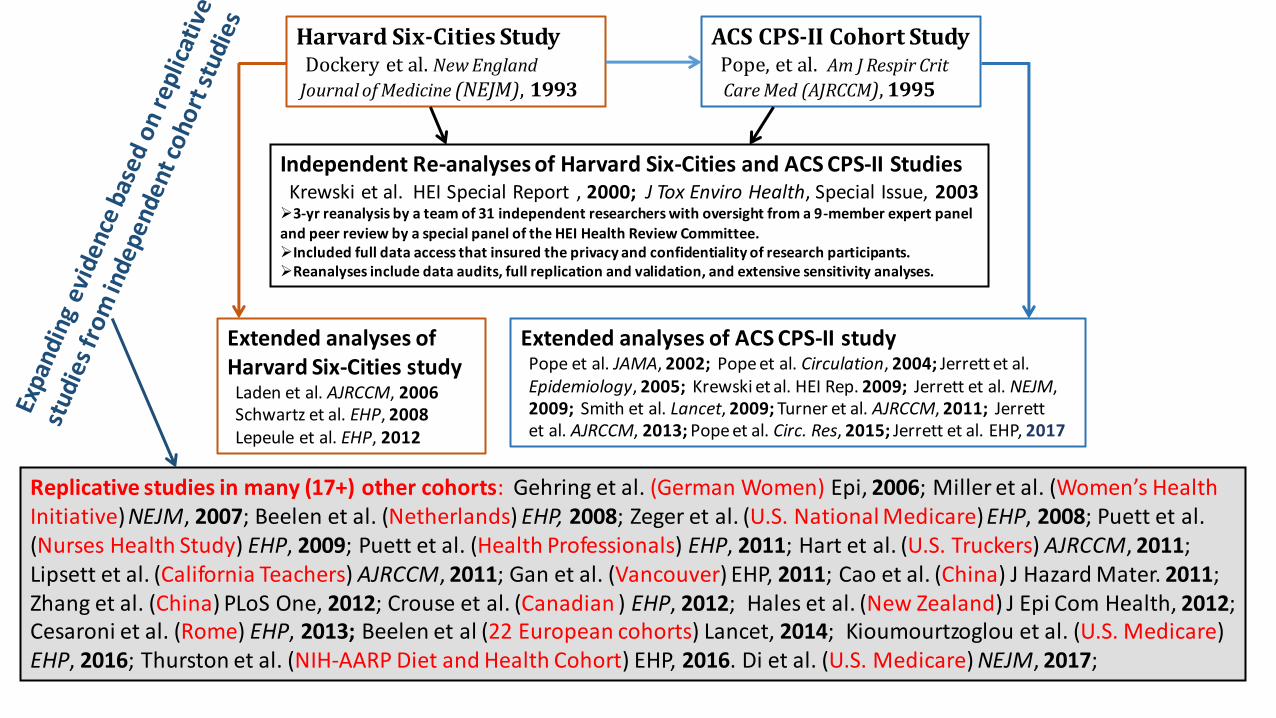
Harvard Six-Cities StudyDockery et al. New England
Journal of Medicine (NEJM), 1993
ACS CPS-II Cohort StudyPope, et al. Am J Respir Crit
Care Med (AJRCCM), 1995
Independent Re-analyses of Harvard Six-Cities and ACS CPS-II StudiesKrewski et al. HEI Special Report , 2000; J Tox Enviro Health, Special Issue, 2003➢3-yr reanalysis by a team of 31 independent researchers with oversight from a 9-member expert panel and peer review by a special panel of the HEI Health Review Committee.➢Included full data access that insured the privacy and confidentiality of research participants.➢Reanalyses include data audits, full replication and validation, and extensive sensitivity analyses.
Extended analyses ofHarvard Six-Cities studyLaden et al. AJRCCM, 2006Schwartz et al. EHP, 2008Lepeule et al. EHP, 2012
Extended analyses of ACS CPS-II studyPope et al. JAMA, 2002; Pope et al. Circulation, 2004; Jerrett et al.Epidemiology, 2005; Krewski et al. HEI Rep. 2009; Jerrett et al. NEJM,2009; Smith et al. Lancet, 2009; Turner et al. AJRCCM, 2011; Jerrettet al. AJRCCM, 2013; Pope et al. Circ. Res, 2015; Jerrett et al. EHP, 2017
Replicative studies in many (17+) other cohorts: Gehring et al. (German Women) Epi, 2006; Miller et al. (Women’s Health Initiative) NEJM, 2007; Beelen et al. (Netherlands) EHP, 2008; Zeger et al. (U.S. National Medicare) EHP, 2008; Puett et al. (Nurses Health Study) EHP, 2009; Puett et al. (Health Professionals) EHP, 2011; Hart et al. (U.S. Truckers) AJRCCM, 2011; Lipsett et al. (California Teachers) AJRCCM, 2011; Gan et al. (Vancouver) EHP, 2011; Cao et al. (China) J Hazard Mater. 2011; Zhang et al. (China) PLoS One, 2012; Crouse et al. (Canadian ) EHP, 2012; Hales et al. (New Zealand) J Epi Com Health, 2012; Cesaroni et al. (Rome) EHP, 2013; Beelen et al (22 European cohorts) Lancet, 2014; Kioumourtzoglou et al. (U.S. Medicare) EHP, 2016; Thurston et al. (NIH-AARP Diet and Health Cohort) EHP, 2016. Di et al. (U.S. Medicare) NEJM, 2017;

Sept. 26, 2017

Key estimated equations:
Mortality or
Life expectancy
for city j.
Indicator variable
equal to 1 for
locations North
of Huai River line
Polynomial
in degrees
North of Huai
River line
Other demographic
and city characteristics
that may effect mortality
Or estimate 2a as the first step in a two stage least-squares (2SLS) and
then estimated 2c above as the second stage equation.


4th Controversy:
So does reducing air pollution improve health and reduce mortality?
3rd Controversy:
Can long-term exposures contribute to significant disease and loss of life?
Answer: Yes


Reduction in fine particulate air pollution:Extended follow-up of the Harvard Six Cities Study(AJRCCM 2006)
0.7
0.8
0.9
1.0
1.1
1.2
1.3
1.4
0 5 10 15 20 25 30 35
PM2.5 (mg/m3)
Mo
rtali
ty R
isk R
ati
o
SteubenvilleTopeka
Watertown
Kingston
St. Louis
Portage
Francine Laden, ScDHarvard
Joel Schwartz, PhDHarvard
Doug Dockery,ScDHarvard
Frank Speizer, MDHarvard

Fine-Particulate Air Pollution and Life Expectancy in the United States
C. Arden Pope, III, Ph.D., Majid Ezzati, Ph.D., and Douglas W. Dockery, Sc.D.
January 22, 2009
Majid Ezzati, PhDImperial College London
Matching PM2.5 data for
1979-1983 and 1999-2000 in51 Metro Areas
Life Expectancy data for1978-1982 and 1997-2001 in
211 counties in 51 Metro areas
Evaluate changes in Life
Expectancy with changes inPM2.5 for the 2-decade period
of approximately 1980-2000.
Francesca Dominici, PhDHarvard

10 µg/m3 decrease in PM2.5 associated with a one year increase in life expectancy.
This increase in life expectancy persisted even after controlling for
socio-economic, demographic, or smoking variables

4th Controversy:
So does reducing air pollution improve health and reduce mortality?
Answer: Yes
5th Controversy:
Does a safe threshold even exist?

Ambient Concentrations ( g/m3)
$
CT
CM
Marginal HealthCosts of Pollution
He
alth
Eff
ect
Health Effect
U.S. CAA requires the EPA to set air quality standards that “are requisite to protect the public health with an adequate margin of safety.”

British Smoke
0 200 400 600 800 1000 1200 1400
Daily
Dea
ths
260
280
300
320
340
360
380
London
Schwartz and Marcus. Am J Epidemiology 1990
Early analyses of concentration-response function.
Used London mortality data for 14 winters
C-R function less steep at higher concentrations
No evidence of a threshold
Joel Schwartz, PhDHarvard
Bart Ostro, PhDUC Davis

PM10
10 20 30 40 50 60 70 80 90
Rela
tive R
isk o
f D
ea
th
0.98
1.00
1.02
1.04
1.06
1.08
1.10
1.12
TSP
60 70 80 90 100 110 120 130
Rela
tive
Ris
k o
f D
ea
th
0.995
1.000
1.005
1.010
1.015
1.020
1.025
PM10
10 15 20 25 30 35 40 45 50
Rela
tive R
isk o
f D
ea
th
0.99
1.00
1.01
1.02
1.03
1.04
1.05
TSP
40 60 80 100 120 140
Rela
tive R
isk o
f D
ea
th
0.99
1.00
1.01
1.02
1.03
1.04
PM10
40 60 80 100 120 140
Rela
tive R
isk o
f D
ea
th
0.98
1.00
1.02
1.04
1.06
1.08
1.10
1.12
1.14
British Smoke
0 200 400 600 800 1000 1200 1400
Daily
Dea
ths
260
280
300
320
340
360
380
LondonA DetroitB
St. LouisC D Utah Valley
E Philadelphia F Sao Paulo
0 20 40 60 80 100
% in
cre
ase
in
de
ath
s
0
2
4
6
8
0 20 40 60 80 100
% in
cre
ase
in
de
ath
s
0
2
4
6
8
0 20 40 60 80 100
% in
cre
ase
in
de
ath
s
0
2
4
6
8
0 20 40 60 80 100 120 140 160 180 200 220%
in
cre
ase
in
de
ath
s
0
2
4
6
8
PM10
(mg/m3)
0 20 40 60 80 100
% in
cre
ase
in
de
ath
s
0
2
4
6
8 10 U.S. Cities
(Schwartz and Zanobetti 2000)a 8 Spanish Cities
(Schwartz et al. 2001)b
20 U.S. Cities
(Daniels et al. 2000;
Dominici et al. 2003)
c d 88 U.S. Cities
(Dominici et al. 2002;
Dominici et al. 2003)
e 22 European Cities
(Samoli et al. 2005)
Figure 1. Selected concentration-response relationships estimated fromvarious multi-city daily time-series mortality studies (approximate adaptationsfrom original publications re-scaled for comparison purposes).
BS (mg/m3)
PM10
(mg/m3) PM
10 (mg/m
3)
PM10
(mg/m3)

5 10 15 20 25 30
0.8
0.9
1.0
1.1
1.2
1.3
1.4
P
T W
L
H
S
p t
w
l
h
s
5 10 15 20 25 30
650
700
750
800
850
900
950
1000
1050
U.S. cross-sectional mortality Harvard Six-cities
(Laden et al. 2006)
5 10 15 20 25 30
Ad
juste
d m
ort
alit
y r
ela
tive r
isk
0.8
0.9
1.0
1.1
1.2
1.3
1.4
5 10 15 20 25 30
FE
V1 <
80
% o
f p
red
icte
d (
%)
0
2
4
6
8
10
12 dc
a b
Figure 2. Selected concentration-response relationships estimated fromvarious studies of long-term exposure (approximate adaptations fromoriginal publications re-scaled for comparison purposes).
PM2.5
(mg/m3)PM
2.5 (mg/m
3)
ACS cohort
(Pope et al. 2002)Children's Lung Growth
(Gauderman et al. 2004)
19
80
ad
juste
d m
ort
alit
y(d
ea
ths/y
r/1
00
,00
0)
Ad
juste
d m
ort
alit
y r
ela
tive r
isk
PM2.5
(mg/m3) PM
2.5 (mg/m
3)
Period 1 (upper case)
Period 2 (lower case)
All cause
Cardiopulmonary
Lung Cancer
All other
Cardiopulmonary Mortality(Pope et al. JAMA 2002)
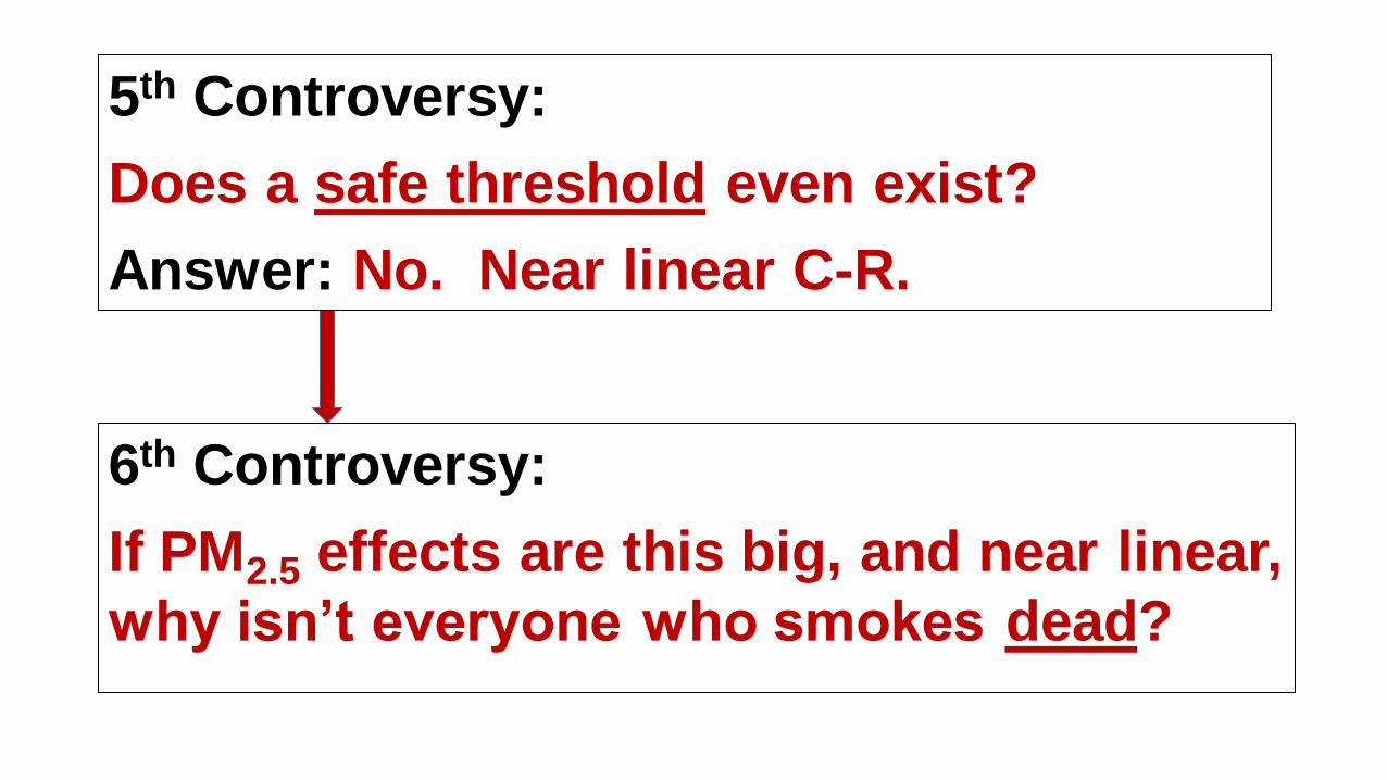
5th Controversy:
Does a safe threshold even exist?
Answer: No. Near linear C-R.
6th Controversy:
If PM2.5 effects are this big, and near linear,
why isn’t everyone who smokes dead?

0 60 120 180 240
Ad
jus
ted
Re
lati
ve
Ris
k
1.0
1.5
2.0
estimated daily dose of PM2.5
, mg
18-22cigs/day
Pack-a-day smoker:
RR ~ 2
Daily inhaled dose ~ 240 mg
Live in polluted city or
With smoking spouse
RR ~ 1.15 – 1.35
Daily inhaled dose ~ 0.2–1.0 mg
Estimated daily dose assumes:
• Inhalation rate of 18 m3/day
• 12 mg/cig
30 µg/m3 of mean PM2.5 X
18 m3/day inhalation rate =540 µg or 0.54 mg daily dose of PM2.5
12 mg/cig X 20 cigs = daily dose of 240 mg PM2.5

0 60 120 180 240 300
Ad
juste
d R
ela
tive R
isk
1.0
1.5
2.0
2.5
<3cigs/day
estimated daily dose of PM2.5
, mg
23+cigs/day
8-12cigs/day
13-17cigs/day
18-22cigs/day
4-7cigs/day
Figure A. Adjusted relative
risks (and 95% CIs) of IHD (light gray), CVD (dark gray), and CPD (black)
mortality plotted over estimated daily dose of
PM2.5 from different increments of current cigarette smoking.
Pope, Burnett, Krewski, et al. 2009.
Estimated daily dose assumes:• Inhalation rate of 18 m3/day • 12 mg/cigarette

0 60 120 180 240 300
Ad
jus
ted
Re
lati
ve
Ris
k
1.0
1.5
2.0
2.5
<3cigs/day
estimated daily dose of PM2.5
, mg
23+cigs/day
8-12cigs/day
13-17cigs/day
18-22cigs/day
4-7cigs/day
Pope, Burnett, Krewski, et al. 2009.Figure 1. Adjusted relative
risks (and 95% CIs) of IHD (light gray), CVD (dark gray), and CPD (black)
mortality plotted over estimated daily dose of
PM2.5 from different increments of current cigarette smoking.
Diamonds represent comparable mortality risk
estimates for PM2.5 from air pollution. Stars represent comparable pooled relative
risk estimates associated with SHS exposure from
the 2006 Surgeon General’s report and from the INTERHEART study.
Estimated daily dose assumes:• Inhalation rate of 18 m3/day • 12 mg/cigarette

0.1 1.0 10.0 100.0
Ad
juste
d R
ela
tive R
isk
1.0
1.5
2.0
2.5
estimated daily dose of PM2.5
, mg
Exposure from
Second hand cigarette smoke: Stars, from 2006 Surgeon General Report and INTERHEART studyAnd air pollution: Hex, from Womens Health Initiative cohort Diamonds, from ACS cohort Triangles, Harvard Six Cities cohort
Exposure from smoking<3, 4-7, 8-12, 13-17, 18-22, and 23+
cigarettes/day
Figure 2. Adjusted relative
risks (and 95% CIs) of ischemic heart disease (light gray), cardiovascular
(dark gray), and cardiopulmonary (black)
mortality plotted over baseline estimated daily dose (using a log scale) of
PM2.5 from current cigarette smoking (relative
to never smokers), SHS, and air pollution.
Pope, Burnett, Krewski, et al. 2009.
Estimated daily dose assumes:• Inhalation rate of 18 m3/day • 12 mg/cigarette

2011

6th Controversy:
If PM2.5 effects are this big, and near linear, why isn’t everyone
who smokes dead?
Answer: Not linear—diminishing marginal effects.
7th Controversy:
Are these health effects biologically plausible?

2004.
RR
(9
5%
CI)
0.65
0.70
0.75
0.80
0.85
0.90
0.95
1.00
1.05
1.10
1.15
1.20
1.25
1.30
1.35
1.40A
ll C
ard
iova
scu
lar
plu
s D
iab
ete
s
Isch
em
ic h
ea
rtd
ise
ase
Dysrh
yth
mia
s,H
ea
rtfa
ilure
, C
ard
iac a
rre
st
Hyp
ert
en
siv
ed
ise
ase
Oth
er
Ath
ero
scle
rosis
,a
ort
ic a
ne
ury
sm
s
Ce
reb
ro-
va
scu
lar
Oth
er
Ca
rdio
-va
scu
lar
Dia
be
tes
Re
sp
ira
tory
Dis
ea
se
s
CO
PD
an
da
llie
d c
on
ditio
ns
Pn
eu
mo
nia
,In
flu
en
za
All
oth
er
resp
ira
tory
Figure 1. Adjusted relative risk ratios for cardiovascular and respiratory mortality associated with
a 10 mg/m3 change in PM
2.5 for 1979-1983, 1999-2000, and the average of the two periods.
(Relative size of the dots correspond to the relative number of deaths for each cause.)
John Godleski, MD
Harvard
Biological mechanisms include:➢ Pulmonary and systemic inflammation➢ Accelerated atherosclerosis➢ Altered cardiac autonomic function
Eugenia Calle, Phd
ACS

Brook, Rajagopalan, Pope, et al. 2011
AHA Scientific Statement, PM and CVD
Robert Brook, MDU of Michigan
Sanjay Rajagopalan, MDUH Cleveland Medical

Fine particulate
exposure(from smoking or air pollution)
↓
Pulmonary and
systemic inflammation
and oxidative stress
(along with blood lipids)
↓
Endothelial
injury/dysfunction
↓
Progression and
destabilization of
atherosclerotic plaques
Consistent with EPI evidence of:
➢ Coronary artery disease➢ Ischemic heart disease events➢ Subsequent heart failure➢ Ischemic strokes➢ Deep vein thrombosis
(and potential pulmonary embolism)

2016Aruni Bhatnagar, PhD FAHAU of Louisville
Tim O’Toole, PhDU of Louisville
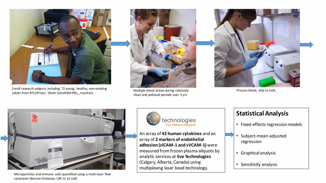
Enroll research subjects including 72 young, healthy, non-smoking adults from BYU/Provo. (Note DataRAM PM2.5 monitor).
Multiple blood draws during relativelyclean and polluted periods over 3 yrs.
Process blood, ship to UofL.
Microparticles and immune cells quantified using a multi-laser flow cytometer (Becton Dickinson LSR II) at UofL
An array of 42 human cytokines and an array of 2 markers of endothelial adhesion (sICAM-1 and sVCAM-1) were measured from frozen plasma aliquots by analytic services at Eve Technologies(Calgary, Alberta, Canada) using multiplexing laser bead technology.
Statistical Analysis
• Fixed-effects regression models
• Subject-mean-adjusted regression
• Graphical analysis
• Sensitivity analysis

1/6 1/13 1/20 1/27 2/3 2/10 2/17 2/24 3/3 3/10 3/17
PM
2.5 (
g/m
3)
0
10
20
30
40
50
60
70
80
90
100
110
120
130
Lindon 1-d FRMNorth Provo 1-d FRMSpanish Fork 1-d FRMLindon 24-h Real timeNorth Provo 24-h Real timeBlood Draws, Subs 1-12
Blood Draws, Subs 13-24
2013
1/5 1/12 1/19 1/26 2/2 2/9 2/16 2/23 3/2 3/9 3/16
PM
2.5 (
g/m
3)
0
10
20
30
40
50
60
70
80
90
100
110
120
130
Lindon 1-d FRMNorth Provo 1-d FRMSpanish Fork 1-d FRMLindon 24-h Real timeNorth Provo 24-h Real timeBlood Draws, Subs 1-12
Blood Draws, Subs 13-24FOB 24-hr Real time
Blood-draw room 24-hr
2014
12/7 12/14 12/21 12/28 1/4 1/11 1/18 1/25 2/1 2/8 2/15 2/22 3/1 3/8 3/15 3/22 3/29 4/5
PM
2.5 (
g/m
3)
0
10
20
30
40
50
60
70
80
90
100
110
120
130
Lindon 1-d FRMNorth Provo 1-d FRMSpanish Fork 1-d FRMLindon 24-h Real timeNorth Provo 24-h Real timeBlood Draws, Subs 1-12
Blood Draws, Subs 13-24
FOB 24-hr Real timeBlood-draw room 24-hr
2014/2015
Figure 1. PM2.5
concentrations and
blood-draw dates
plotted during study
periods.

Elevated
circulating
endothelial
microparticles
indicative of
endothelial cell
apoptosis and
endothelial
injury.
Elevated circulating monocytes and T,
but not B, lymphocytes—Suggestive
of a non-specific or innate immune
response and not a specific adaptive
response involving production of
antibodies targeting specific antigens.
Weaker but sig. association with
platelet-monocyte aggregates

%
-8
-6
-4
-2
0
2
4
6
8
10
12
14
16
TN
F
sIC
AM
-1
MC
P-1
IL-8
Fra
cta
lkin
e
MIP
-1
MIP
-1
IP-1
0
sV
CA
M-1
IL-6
IL-1
0
IL-1
IL-9
IL-1
5
IL-1
RA
IL-1
3
IL-1
2P
70
G-C
SF
Eo
taxi
n-1
IL-5
IL-1
TN
F
MC
p-3
IL-1
2P
40
FG
F-2
TG
F
GM
-CS
F
IL-1
7A
IL-2
IL-7
IFN
y
IL-4
PD
GF
-BB
Flt-3
L
IL-1
8
MD
C
IFN
2
IL-3
VE
GF
-A
GR
O
RA
NT
ES
PD
GF
-AA
sC
D4
0L
EG
F
Figure 3. Percent change (and 95% CIs) in analyte per 10 g/m3 increase in PM
2.5 relative to mean value
of analyte. Estimates come from subject-mean adjusted regressions. The results are ordered from left to
right based on t-values--resulting in the most statistically signifiant possitive associations being on the left
and the most statistially significant negative associations being on the right.
Statistically significant even when
using the Bonferroni correction for
multiple testing of 44 analytes (P<0.05/44)
Statistical interpretation

%
-8
-6
-4
-2
0
2
4
6
8
10
12
14
16T
NF
sIC
AM
-1
MC
P-1
IL-8
Fra
cta
lkin
e
MIP
-1
MIP
-1
IP-1
0
sV
CA
M-1
IL-6
IL-1
0
IL-1
IL-9
IL-1
5
IL-1
RA
IL-1
3
IL-1
2P
70
G-C
SF
Eo
taxi
n-1
IL-5
IL-1
TN
F
MC
p-3
IL-1
2P
40
FG
F-2
TG
F
GM
-CS
F
IL-1
7A
IL-2
IL-7
IFN
y
IL-4
PD
GF
-BB
Flt-3
L
IL-1
8
MD
C
IFN
2
IL-3
VE
GF
-A
GR
O
RA
NT
ES
PD
GF
-AA
sC
D4
0L
EG
F
Figure 3. Percent change (and 95% CIs) in analyte per 10 g/m3 increase in PM
2.5 relative to mean value
of analyte. Estimates come from subject-mean adjusted regressions. The results are ordered from left to
right based on t-values--resulting in the most statistically signifiant possitive associations being on the left
and the most statistially significant negative associations being on the right.
Increase in proinflammatory/
anti-angiogenic cytokines (TNFα,
monocyte chemoattractant protein 1,
IL-8, macrophage inflammatory
protein 1α/β, interferon γ-induced
protein 10)
Suppressed cytokines/ growth
factors that are potent
pro-angiogenic factors,
including: epidermal growth
factor, CD40 ligand, platelet-
derived growth factor, RANTES,
growth-regulated protein alpha,
and vascular endothelial growth
factor.
Anti-angiogenic plasma profile
Elevated intercellular adhesion molecule 1
and vascular cellular adhesion molecule 1.


7th Controversy:
Are these health effects biologically plausible?
Answer: There are plausible biological mechanisms.
8th Controversy:
Aren’t air pollution health effects just small compared to other more important risk factors.

The Global Burden of Disease 2010
Bre
ath
ing
Co
nta
min
ants
Christopher Murray, MDU of Washington, IHME
Aaron Cohen, DSc.HEI, IHME
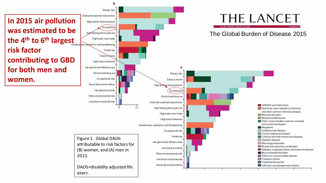
The Global Burden of Disease 2015
Figure 1. Global DALYs attributable to risk factors for (B) women, and (A) men in 2015.
DALYs=disability adjusted life years.
In 2015 air pollution was estimated to be the 4th to 6th largest risk factor contributing to GBD for both men and women.

The Global Burden of Disease 2015
Breathing contaminants contributes to global burden of disease (GBD)
Number of attributable deaths
Tobacco Smoking 6.4 mil.
Second Hand Smoke 0.9 mil.
PM2.5 air pollution 4.2 mil.
Household air pollution from solid fuels 2.9 mil.
Ambient Ozone 0.2 mil.

8th Controversy:
Aren’t air pollution health effects just small compared to other more important risk factors.
Answer: No. The effects of air pollution as substantial.
9th Controversy:
Cleaning up air pollution costs too much and hurts our economy.

Clean versus
polluted air is
among our
economic
choices.
➢ Clean air is an economic good that contributes to human
well-being, human capital, and positive environmental
amenities.
➢ The “production” of clean air can contribute to economic
prosperity, human well being, and improved public health.
Medellin

Changes in Economic Indicators and Pollutant Emissions 1970-2015. Adapted from Samet et al. NEJM March 1, 2017.
Gross domestic product
Vehicle miles traveled
Population
Energy consumption
CO2 emissions
Aggregate air pollutionemissions (6 common pol.)
1970CAA
&EPA

U.S. EPA March 2011

10th Controversy: How much evidence is needed before efforts to have clean air are no longer controversial?

Economics Principles ofAir Pollution Management

Over London by Rail, 1870
Gustave DoréDepicts the congested and pollutedIndustrial environment of 1870 London

Classical Economics
• Adam Smith (Scottish social philosopher and political economist), author of Wealth of Nations (1776), free markets,
competition, and the metaphor of the
“invisible hand”.
• Doctrine of “Laissez-faire”
• What about air pollution? Smells like money to me!

Began to lose our Faith in the doctrine of Laissez-fair
Dec. 5-9, 1952: London--1000’s of excess deaths
Dec. 1-5, 1930: Meuse Valley, Belgium60 deaths (10x expected)
Oct. 27-31, 1948: Donora, PA20 deaths, ½ the town’s population fell ill
Respiratory and cardiovascular disease and death

Loss of Faith in the doctrine of Laissez-faire
• No longer did air pollution “smell like money” but it smelled like something unhealthy.
• In the UK, US, and elsewhere public policy efforts to clean up the air and eliminate the “Killer Smog Episodes” began (Clean air act).
• There was success at eliminating or reducing the extreme air pollution episodes but air pollution remained and we have learned that even moderate air pollution had adverse health effects.

Ambient Concentrations ( g/m3)
$
CT
CM
Marginal HealthCosts of Pollution

Ambient Concentrations ( g/m3)
$
Marginal Costof Abatement
Marginal Health Costof Pollution
CT C* C
M

Ambient Concentrations ( g/m3)
$
Marginal Costof Abatement
Marginal Health Costof Pollution
CT C* C
M
Management approach 1—Do nothing

Ambient Concentrations ( g/m3)
$
Marginal Costof Abatement
Marginal Health Costof Pollution
CT C* C
M
DEAD WEIGHT LOSS(due to over abatement)
Management approach 2—Abate pollution at or below threshold

Ambient Concentrations ( g/m3)
$
Marginal Costof Abatement
Marginal Health Costof Pollution
CT C* C
M
Re
gula
tory
act
ion
1 (
ban
co
al/w
oo
d b
urn
ing
for s
pac
e h
eat
ing)
Re
gula
tory
act
ion
2 (
stag
e I
auto
em
issi
on c
on
tro
ls)
Re
gula
tory
act
ion
3 (
coal
po
we
r pla
nt c
on
tro
ls)
Re
gula
tory
act
ion
5
(sta
ge II
au
to e
mis
sion
co
ntr
ols
)
Re
gula
tory
act
ion
4 (
ste
el
mil
l/sm
elte
r em
issi
on
con
tro
ls)
RA 6 (Dieselemission controls)
Management approach 3—Use regulatory actions and B/C criteria

Ambient Concentrations ( g/m3)
$
Marginal Costof Abatement
Marginal Health Costof Pollution
CT C* C
M
Re
gula
tory
act
ion
1 (
ban
co
al/w
oo
d b
urn
ing
for s
pac
e h
eat
ing)
Re
gula
tory
act
ion
2 (
stag
e I
auto
em
issi
on c
on
tro
ls)
Re
gula
tory
act
ion
3 (
coal
po
we
r pla
nt c
on
tro
ls)
Re
gula
tory
act
ion
5
(sta
ge II
au
to e
mis
sion
co
ntr
ols
)
Re
gula
tory
act
ion
4 (
ste
el
mil
l/sm
elte
r em
issi
on
con
tro
ls)
RA 6 (Dieselemission controls)
Assumes regulatory management that is wise, competent, well-enforced, efficient, not over reaching,politically acceptable, etc.

Ambient Concentrations ( g/m3)
$
Marginal Costof Abatement
Marginal Health Costof Pollution
CT C* C
M
Piqovian Tax rate or Price in Cap-and-Trade scheme.
Management approach 4 and 5—Use Pigovian Taxes or Cap-and Trade

Ambient Concentrations ( g/m3)
$
Marginal Costof Abatement
Marginal Health Costof Pollution
CT C* C
M
Piqovian Tax rate or Price in Cap-and-Trade scheme.
Also assumes management and enforcement of the Piqovian Tax or the Cap-and-Trade scheme that is feasible, enforceable, politically acceptable, etc.

In Six-Cities study, adjusted relative risk of dying werealmost linearly associated with air pollution.

In ACS study, adjusted relative risk of dying were
almost linearly associated with air pollution.

Ambient Concentrations ( g/m3)
$
Marginal Costof Abatement
Marginal Health Costof Pollution
C*

Ambient Concentrations ( g/m3)
$
Marginal Costof Abatement
Marginal HealthCost of Pollution
C*
high estimate
median estimate
low estimate
CL C
H

0 60 120 180 240 300
Ad
jus
ted
Re
lati
ve
Ris
k
1.0
1.5
2.0
2.5
<3cigs/day
estimated daily dose of PM2.5
, mg
23+cigs/day
8-12cigs/day
13-17cigs/day
18-22cigs/day
4-7cigs/day
Pope, Burnett, Krewski, et al. 2009.
Figure 1. Adjusted relative
risks (and 95% CIs) of IHD (light gray), CVD (dark gray), and CPD (black)
mortality plotted over estimated daily dose of
PM2.5 from different increments of current cigarette smoking.
Diamonds represent comparable mortality risk
estimates for PM2.5 from air pollution. Stars represent comparable pooled relative
risk estimates associated with SHS exposure from
the 2006 Surgeon General’s report and from the INTERHEART study.

Ambient Concentrations ( g/m3)
$
C* CH
Marginal Costsof Abatement
Marginal HealthCosts of Pollution
CNC
Pollution Abatement

Ambient Concentrations ( g/m3)
$
C* CH
Marginal Costsof Abatement
Marginal HealthCosts of Pollution
CNC

Ambient Concentrations ( g/m3)
$
C* CH
Marginal Costsof Abatement
Marginal HealthCosts of Pollution
CNC

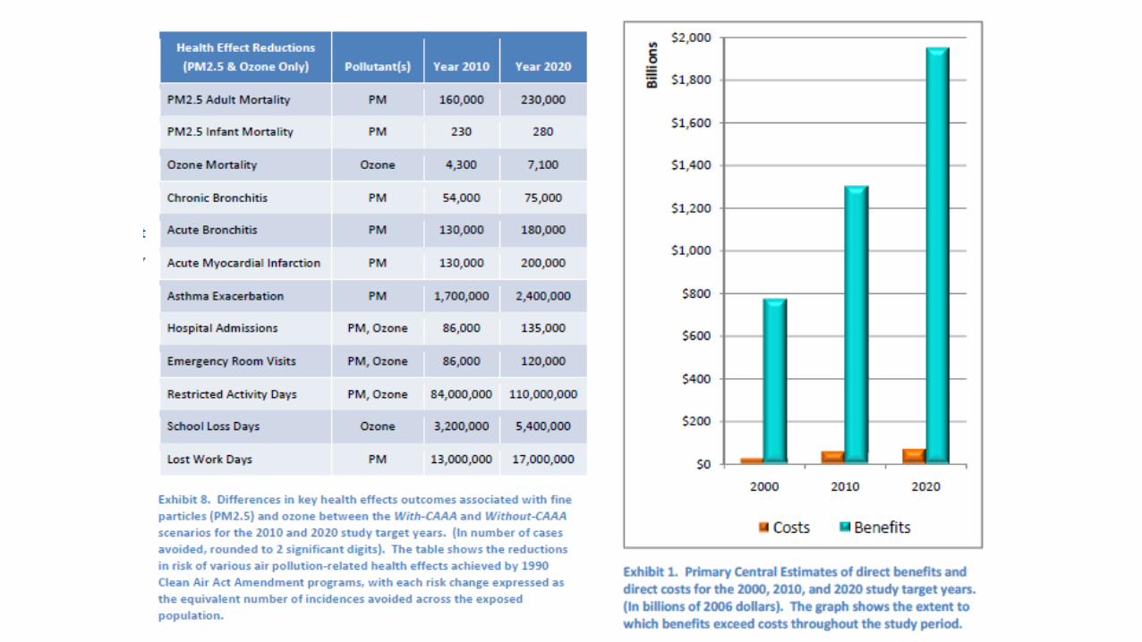
In 2007 and 2008 OMB estimates that the
largest benefits of ALL federal regulations were
attributable to controlling exposure to a single
air pollutant:
fine particulate matter (PM2.5).
Estimated benefits:
$18.8 to $167.4 billion/year
Estimated costs:
$7.3 billion per/year


Ambient Concentrations ( g/m3)
$
C* CH
Marginal Costsof Abatement
Marginal HealthCosts of Pollution
CNC

ER = 0.0063 * (PM2.5)
(Approximately from Hoek et al., 2013)
ER = 0.4 {1 – exp [-.03 (PM2.5)0.9 ] }
(Approximation based on functional form of the integrated risk function, Burnett et al. 2014).
Figure 2. Stylized analysis of pollution abatement for linear and supralinear C-R functions.
From:Pope, Cropper, Coggins, Cohen. JAWMA 2015

Fine-Particulate Air Pollution and Life Expectancy in the United States
C. Arden Pope, III, Ph.D., Majid Ezzati, Ph.D., and Douglas W. Dockery, Sc.D.
January 22, 2009
Matching PM2.5 data for1979-1983 and 1999-2000 in
51 Metro Areas
Life Expectancy data for
1978-1982 and 1997-2001 in 211 counties in 51 Metro areas
Evaluate changes in Life
Expectancy with changes in
PM2.5 for the 2-decade periodof approximately 1980-2000.
0 2 4 6 8 10 12 14
0
5
10
15
20
Reduction in PM2.5 (mg/m3)
Incr
eas
e in
inco
me
($
10
00
s)
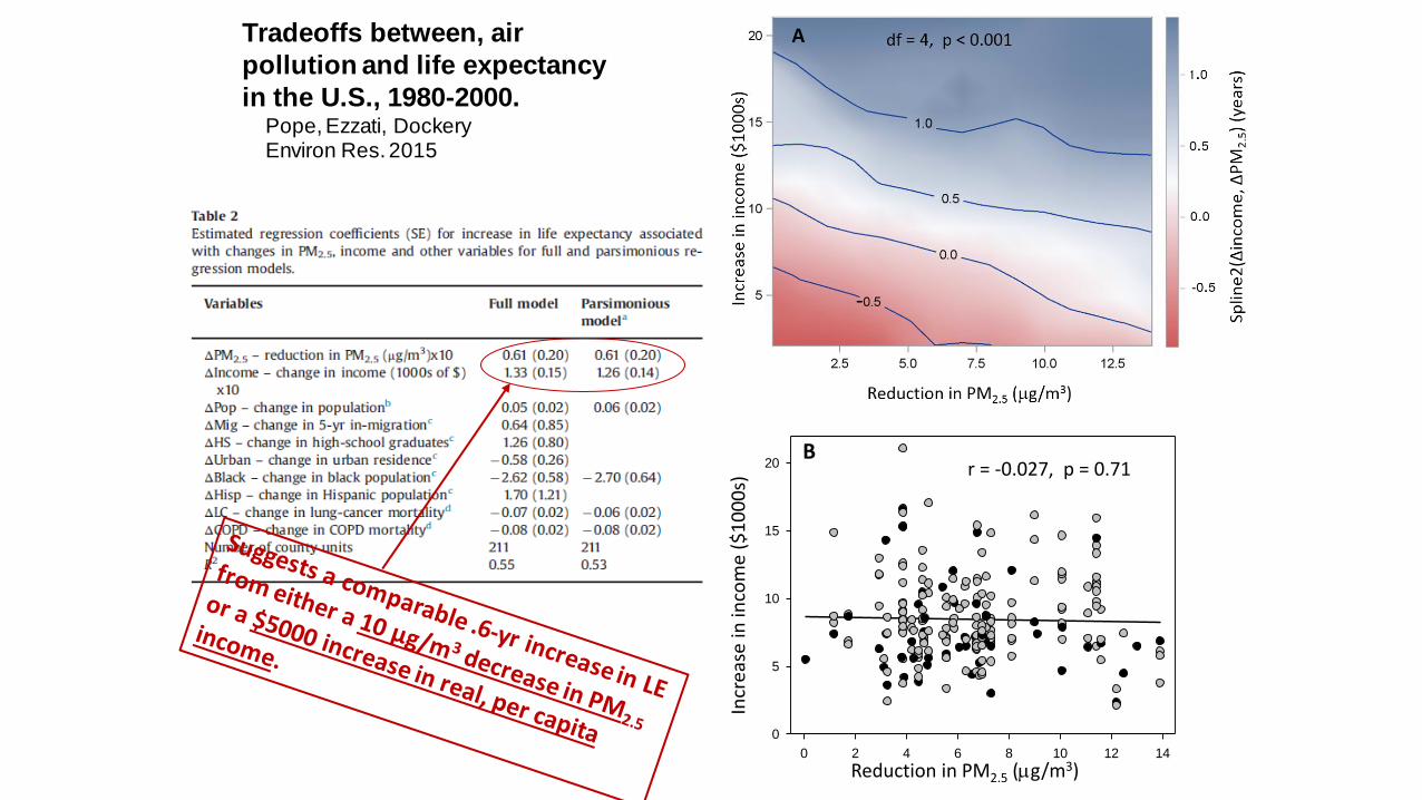
Br = -0.027, p = 0.71
Tradeoffs between, air
pollution and life expectancy
in the U.S., 1980-2000.Pope, Ezzati, DockeryEnviron Res. 2015

Changes in Economic Indicators and Pollutant Emissions 1970-2015.Adapted from Samet et al. NEJM March 1, 2017.
GDP
Vehicle miles traveled
Population
Energy consumption
CO2 emissions
Aggregate air pollutionEmissions(6 common pol.)
1970CAA
&EPA

Clean versus
polluted air is
among our
economic
choices.
➢ Clean air is an economic good that contributes to human
well-being, human capital, and positive environmental
amenities.
➢ The “production” of clean air can contribute to economic
prosperity, human well being, and improved public health.
Medellin

Finally,
This stylized approach ignores various uncertainties and complications including:
➢Interactive multi-pollutants,
➢Issues of environmental justice,
➢How do efforts to reduce traditional air pollutants complement or diverge from efforts to address climate change and is there a reasonable way to integrate these efforts.
Thank you.