relations between reflection and transmission responses of three

Geophys. J. Int. (2004) 156, 179–194 doi: 10.1111/j.1365-246X.2003.02152.x

GJI

Geo

desy

,pot

ential

fiel

dan

dap

plie

dge

ophy

sics

Relations between reflection and transmission responsesof three-dimensional inhomogeneous media

Kees Wapenaar, Jan Thorbecke and Deyan DraganovCentre for Technical Geoscience, Delft University of Technology, PO Box 5028, 2600 GA Delft, the Netherlands. E-mail: [email protected]

Accepted 2003 September 30. Received 2003 September 16; in original form 2002 October 10

S U M M A R YRelations between reflection and transmission responses of horizontally layered media wereformulated by Claerbout in 1968 and by many others. In this paper we derive similar relationsfor 3-D inhomogeneous media. As the starting point for these derivations, we make use oftwo types of propagation invariants, based on one-way reciprocity theorems of the convolu-tion type and of the correlation type. We obtain relations between reflection and transmissionresponses, including their codas, due to internal multiple scattering. These relations can beused for deriving the reflection response from transmission measurements (which is useful forseismic imaging of the subsurface, using passive recordings of noise sources in the subsur-face, also known as acoustic daylight imaging) as well as for deriving the transmission codafrom the reflection measurements (which is useful for seismic imaging schemes that take in-ternal multiple scattering into account). Furthermore, following the same approach, we obtainmutual relations between reflection responses with and without free-surface multiples. Theconvolution-type relations are similar to those used by Berkhout and others for surface-relatedmultiple elimination, whereas the correlation-type relations resemble Schuster’s relations forseismic interferometry. Last, but not least, we obtain expressions for the reflection response ata boundary below an inhomogeneous medium, which may be useful for imaging the medium‘from below’. The main text of this paper deals with the acoustic situation; the Appendicesprovide extensions to the elastodynamic situation.

Key words: acoustic daylight imaging, coda, propagation invariant, reciprocity, seismicinterferometry.

I N T RO D U C T I O N

In this paper we present a unified approach for deriving relationships between seismic reflection and transmission responses in 3-D inhomo-geneous acoustic and full elastic media. In all relations, the codas due to internal multiple scattering are included. We consider situations withand without a free surface on top of the configuration; below a specific depth level we assume that the medium is homogeneous. Hence, theresponses of interest are:

(1) reflection responses at the upper boundary, with and without free-surface multiples at the upper boundary;(2) transmission responses between the upper and lower boundaries, with and without free-surface multiples at the upper boundary;(3) reflection responses at the lower boundary, with and without free-surface multiples at the upper boundary.

Apart from relations between reflection and transmission responses we will encounter relations between reflection responses with and withoutfree-surface multiples and relations between reflection responses at the upper and lower boundaries.

The relations between reflection and transmission responses are the basis for deriving the reflection response from the transmissionresponse, and the coda of the transmission response from the reflection response. The former relation is relevant for ‘acoustic daylightimaging’, that is, for imaging the subsurface from passive recordings of the transmission responses of natural noise sources in the subsurface(Rickett and Claerbout 1999). The latter relation is useful for deriving seismic imaging schemes that take internal multiple scattering intoaccount.

The relations between reflection responses with and without free-surface multiples are the basis for surface-related multiple elimination(Verschuur et al. 1992; van Borselen et al. 1996) as well as for interferometric imaging, that is, imaging the subsurface from cross-correlateddata (Schuster 2001).

C© 2003 RAS 179

Dow

nloaded from https://academ

ic.oup.com/gji/article/156/2/179/2044909 by guest on 14 D

ecember 2021

180 K. Wapenaar, J. Thorbecke and D. Draganov

Finally, the relations between reflection responses at the upper and lower boundaries may prove to be useful for imaging the medium‘from below’, in addition to conventional imaging ‘from above’.

Similar relations have been obtained by many authors for acoustic as well as elastodynamic waves in horizontally layered media. Wemention Claerbout (1968), Frasier (1970), Kennett et al. (1978), Ursin (1983) and Chapman (1994). In the main text of this paper we derivethe relations for 3-D inhomogeneous acoustic media. In Appendix A we generalize the results for the full elastic situation.

P RO PA G AT I O N I N VA R I A N T S A N D R E C I P RO C I T Y T H E O R E M S

Haines (1988), Kennett et al. (1990), Koketsu et al. (1991) and Takenaka et al. (1993) used ‘propagation invariants’ for 3-D inhomogeneousacoustic and elastic media as the starting point for deriving symmetry properties of reflection and transmission responses as well as fordesigning efficient numerical modelling schemes. For the acoustic situation the propagation invariant in the space–frequency domain is givenby∫

�

{PAV3,B − V3,A PB} d2x, (1)

where � is an arbitrary horizontal integration boundary, P = P(x, ω) and V 3 = V 3(x, ω) denote the acoustic pressure and the verticalcomponent of the particle velocity, ω denotes the angular frequency, and x = (x 1, x 2, x 3) the Cartesian coordinate vector (throughout thispaper the x3-axis points downwards). The subscripts A and B refer to two independent acoustic states. The notion ‘propagation invariant’refers to the fact that the quantity described by eq. (1) does not change when the depth level of � is varied. This is true for lossless as well asdissipative media; the only condition is that � should not encounter any sources on its journey. Hence, for a source-free 3-D inhomogeneousregion enclosed by horizontal boundaries ∂D0 and ∂Dm, we can write∫

∂D0

{PAV3,B − V3,A PB} d2x =∫

∂Dm

{PAV3,B − V3,A PB} d2x. (2)

The procedure for deriving the symmetry properties of reflection and transmission responses employed by the above-mentioned authors canbe summarized as follows.

(1) Apply plane-wave decomposition to all the wavefields in eq. (2) and use Parseval’s theorem to transform eq. (2) to the horizontalwavenumber domain.

(2) Assume that the inhomogeneous region is embedded between homogeneous half-spaces above ∂D0 and below ∂Dm. Express thewavefields in the transformed eq. (2) in terms of downgoing and upgoing waves, using wavefield decomposition operators.

(3) Introduce reflection and transmission operators that interrelate the downgoing and upgoing wavefields in the transformed eq. (2). Withthese substitutions, eq. (2) leads to symmetry relations for the reflection and transmission responses defined at the boundaries ∂D0 and ∂Dm

of the inhomogeneous region.(4) Optionally, when the inhomogeneous region only contains a mildly curved interface that obeys the conditions for the validity of the

Rayleigh hypothesis, the integration boundaries ∂D0 and ∂Dm can be moved to one and the same depth level between the boundaries, withoutchanging the character of the downgoing and upgoing waves under the integrals. This leads to symmetry relations for the reflection andtransmission responses of the curved interface, all defined at the same depth level.

It is worth noting that the propagation invariant can be seen as a special case of Rayleigh’s acoustic reciprocity theorem (de Hoop 1988). Sincereciprocity theorems have been derived in various forms, this enables us to formulate a number of alternatives for eq. (2) that have not beenconsidered by the authors mentioned above.

First of all, we can distinguish between reciprocity theorems of the convolution-type and of the correlation-type (Bojarski 1983). Eq. (2)is a special case of the convolution-type reciprocity theorem (the products PAV 3,B etc. in the frequency domain correspond to convolutions inthe time domain). From the reciprocity theorem of the correlation-type we obtain∫

∂D0

{P∗

A V3,B + V ∗3,A PB

}d2x =

∫∂Dm

{P∗

A V3,B + V ∗3,A PB

}d2x, (3)

where ∗ denotes complex conjugation (the products P∗AV 3,B etc. in the frequency domain correspond to correlations in the time domain).

Again, the medium between ∂D0 and ∂Dm is arbitrarily inhomogeneous and source-free. Unlike eq. (2), which is valid for lossless as well asdissipative media, however, eq. (3) is valid only for lossless media.

Furthermore, reciprocity theorems can be formulated in terms of two-way and one-way wavefields. Eqs (2) and (3) are both expressed interms of two-way wavefields. Reciprocity theorems for one-way (that is, downgoing and upgoing) wavefields have been derived by Wapenaar& Grimbergen (1996). For these one-way reciprocity theorems, too, we distinguish between a convolution-type and a correlation-type theorem.From the reciprocity theorem of the convolution-type for one-way wavefields we obtain, analogous to eq. (2),∫

∂D0

{P+

A P−B − P−

A P+B

}d2x =

∫∂Dm

{P+

A P−B − P−

A P+B

}d2x, (4)

where P+ = P+(x, ω) and P− = P−(x, ω) are flux-normalized downgoing and upgoing wavefields, respectively. Eq. (4) holds for primaryand multiply reflected waves with any propagation angle (including evanescent wave modes) in 3-D lossless or dissipative inhomogeneous

C© 2003 RAS, GJI, 156, 179–194

Dow



ecember 2021

Reflection and transmission responses 181

media. Finally, from the one-way reciprocity theorem of the correlation-type we obtain, analogous to eq. (3),∫∂D0

{(P+

A )∗ P+B − (P−

A )∗ P−B

}d2x =

∫∂Dm

{(P+

A )∗ P+B − (P−

A )∗ P−B

}d2x. (5)

Here it is assumed that the medium is lossless and that evanescent wave modes can be neglected. As a consequence, any result obtained fromeq. (5) will be spatially band-limited (we will see an effect of this in Fig. 3b). In what follows, when we speak of two-way reciprocity theoremswe refer to eqs (2) and (3), whereas when we speak of one-way reciprocity theorems we refer to eqs (4) and (5).

In this paper we will use the convolution-type and correlation-type one-way reciprocity theorems with various combinations of boundaryconditions to derive relations between reflection and transmission responses. The choice for the one-way theorems is mainly a matter ofconvenience. Since reflection and transmission responses can be seen as transfer functions between downgoing and/or upgoing one-waywavefields, the one-way reciprocity theorems lead in a straightforward manner to relations between these responses. For example, fromthe step-wise procedure discussed above, only step 3 is required [with eq. (2) in the wavenumber domain replaced by eq. (4) in the spacedomain] to establish the symmetry relations for the reflection and transmission responses. This is reviewed in the section ‘source–receiverreciprocity’. Our use of correlation-type reciprocity theorems leads to results that are essentially different from those derived by the authorsmentioned at the beginning of this section. Furthermore, by employing various combinations of boundary conditions (see the next section)we differentiate from previous work. As a result, we obtain a number of new relations between reflection and transmission responses thatlead to a number of potential applications in seismic processing. One of the applications, acoustic daylight imaging, will be discussed indetail.

S P E C I F I C AT I O N O F T H E S TAT E S F O R T H E O N E - WAY R E C I P RO C I T Y T H E O R E M S

In this section we define the states A and B that will be used in the one-way reciprocity theorems for deriving the relations between thereflection and transmission responses. As mentioned in the Introduction, we consider responses with and without free-surface multiples. Forthe situation without free-surface multiples, consider the configuration denoted as State A−1 in Fig. 1. The boundaries ∂D0 and ∂Dm arechosen at depth levels x 3,0 + ε and x3,m − ε, respectively (with x 3,m > x 3,0 and ε a vanishing positive constant). The half-spaces above ∂D0

and below ∂Dm are homogeneous; the medium in domain D between boundaries ∂D0 and ∂Dm is 3-D inhomogeneous and source-free. We

Figure 1. States for the acoustic one-way reciprocity theorems. State A-1: at xA just above ∂D0 there is a source of downgoing waves. The half-spaces above∂D0 and below ∂Dm are homogeneous. The half-space below ∂Dm is source-free. State A-2: as state A-1, but with a source of upgoing waves at x′

A just below∂Dm. State A-3: as state A-1, but with a free surface just above ∂D0. State A-4: as state A-3, but with a source of upgoing waves at x′

A just below ∂Dm.

C© 2003 RAS, GJI, 156, 179–194

Dow



ecember 2021


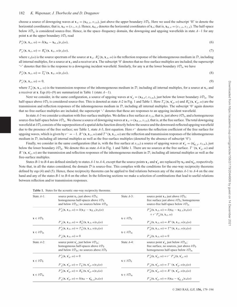
choose a source of downgoing waves at x A = (xH,A, x 3,0), just above the upper boundary ∂D0. Here we used the subscript ‘H’ to denote thehorizontal coordinates; that is, xH = (x 1, x 2). Hence, xH,A denotes the horizontal coordinates of xA; that is, xH,A = (x 1,A, x 2,A). The half-spacebelow ∂Dm is considered source-free. Hence, in the space–frequency domain, the downgoing and upgoing wavefields in state A−1 for anypoint x at the upper boundary ∂D0 read

P+A (x, xA, ω) = δ(xH − xH,A)sA(ω), (6)

P−A (x, xA, ω) = R+

0 (x, xA, ω)sA(ω), (7)

where sA(ω) is the source spectrum of the source at x A. R+0 (x, x A, ω) is the reflection response of the inhomogeneous medium in D, including

all internal multiples, for a source at xA and a receiver at x. The subscript ‘0’ denotes that no free-surface multiples are included; the superscript‘+’ denotes that this is the response to a downgoing incident wavefield. Similarly, for any x at the lower boundary ∂Dm we have

P+A (x, xA, ω) = T +

0 (x, xA, ω)sA(ω), (8)

P−A (x, xA, ω) = 0, (9)

where T +0 (x, x A, ω) is the transmission response of the inhomogeneous medium in D, including all internal multiples, for a source at xA and

a receiver at x. Eqs (6)–(9) are summarized in Table 1 (state A−1).Next we consider, in the same configuration, a source of upgoing waves at x′

A = (xH,A′, x3,m), just below the lower boundary ∂Dm. Thehalf-space above ∂D0 is considered source-free. This is denoted as state A-2 in Fig. 1 and Table 1. Here T −

0 (x, x′A, ω) and R−

0 (x, x′A, ω) are the

transmission and reflection responses of the inhomogeneous medium in D, including all internal multiples. The subscript ‘0’ again denotesthat no free-surface multiples are included; the superscript ‘-’ denotes that these are responses to an upgoing incident wavefield.

In state A-3 we consider a situation with free-surface multiples. We define a free surface at x3,0, that is, just above ∂D0, and a homogeneoussource-free half-space below ∂Dm. We choose a source of downgoing waves at x A = (xH,A, x 3,0), that is, at the free surface. The total downgoingwavefield at ∂D0 consists of the superposition of a spatial delta function directly below the source and the downward-reflected upgoing wavefielddue to the presence of the free surface; see Table 1, state A-3, first equation. Here r− denotes the reflection coefficient of the free surface forupgoing waves, which is given by r− = −1. R+(x, x A, ω) and T +(x, x A, ω) are the reflection and transmission responses of the inhomogeneousmedium in D, including all internal multiples as well as the free-surface multiples (denoted by the absence of subscript ‘0’).

Finally, we consider in the same configuration (that is, with the free surface at x3,0) a source of upgoing waves at x′A = (x′

H,A, x3,m), justbelow the lower boundary ∂Dm. We denote this as state A-4 in Fig. 1 and Table 1. There are no sources at the free surface. T −(x, x′

A, ω) andR−(x, x′

A, ω) are the transmission and reflection responses of the inhomogeneous medium in D, including all internal multiples as well as thefree-surface multiples.

States B-1 to B-4 are defined similarly to states A-1 to A-4, except that the source points xA and x′A are replaced by xB and x′

B , respectively.Note that, in all the states considered, the domain D is source-free. This complies with the conditions for the one-way reciprocity theoremsdefined by eqs (4) and (5). Hence, these reciprocity theorems can be applied to find relations between any of the states A-1 to A-4 on the onehand and any of the states B-1 to B-4 on the other. In the following sections we make a selection of combinations that lead to useful relationsbetween reflection and/or transmission responses.

Table 1. States for the acoustic one-way reciprocity theorems.

State A-1: source point xA just above ∂D0; State A-3: source point xA just above ∂D0;homogeneous half-spaces above ∂D0 free surface just above ∂D0; homogeneousand below ∂Dm; no sources below ∂Dm source-free half-space below ∂Dm

P+A (x, x A , ω) = δ(xH − xH,A)sA(ω) P+

A (x, x A , ω) = δ(xH − xH,A)sA(ω)

+ r−P−A (x, xA, ω)

x ∈ ∂D0 x ∈ ∂D0

P−A (x, x A , ω) = R+

0 (x, x A , ω)sA(ω) P−A (x, x A , ω) = R+(x, x A , ω)sA(ω)

P+A (x, x A , ω) = T +

0 (x, x A , ω)sA(ω) P+A (x, x A , ω) = T +(x, x A , ω)sA(ω)

x ∈ ∂Dm x ∈ ∂Dm

P−A (x, x A , ω) = 0 P−

A (x, x A , ω) = 0

State A-2: source point x′A just below ∂Dm; State A-4: source point x′

A just below ∂Dm;homogeneous half-spaces above ∂D0 free surface, no sources, just above ∂D0

and below ∂Dm; no sources above ∂D0 homogeneous half-space below ∂Dm

P+A (x, x′

A , ω) = 0 P+A (x, x′

A , ω) = r− P−A (x, x′

A , ω)

x ∈ ∂D0 x ∈ ∂D0

P−A (x, x′

A , ω) = T −0 (x, x′

A , ω)sA(ω) P−A (x, x′

A , ω) = T −(x, x′A , ω)sA(ω)

P+A (x, x′

A , ω) = R−0 (x, x′

A , ω)sA(ω) P+A (x, x′

A , ω) = R−(x, x′A , ω)sA(ω)

x ∈ ∂Dm x ∈ ∂Dm

P−A (x, x′

A , ω) = δ(xH − x′H,A)sA(ω) P−

A (x, x′A , ω) = δ(xH − x′

H,A)sA(ω)

C© 2003 RAS, GJI, 156, 179–194

Dow



ecember 2021


S O U RC E – R E C E I V E R R E C I P RO C I T Y

In this section we derive source–receiver reciprocity relations. Although these relations are well known for full wavefields (that is, solutionsof the two-way wave equation), they are less obvious for one-way wavefields (that is, solutions of the coupled one-way wave equations fordowngoing and upgoing waves). Note that, if pressure-normalization were used instead of flux-normalization for the decomposition of the fullwavefield into one-way wavefields in inhomogeneous media, reciprocity would not hold for the one-way wavefields. Flux-normalization wasused in the derivation of the one-way reciprocity theorems (4) and (5), which explains their relatively simple form. We will now demonstrate thatthese theorems lead to source–receiver reciprocity relations for the reflection and transmission responses introduced in the previous section.

We substitute the expressions for the one-way wavefields of states A-1 and B-1 (Table 1) into the one-way convolution-type reciprocitytheorem (eq. 4). Dividing the result by sA(ω)sB(ω) we obtain∫

∂D0

[δ(xH − xH,A)R+

0 (xH, x3,0, xB, ω) − R+0 (xH, x3,0, xA, ω)δ(xH − xH,B)

]d2x = 0, (10)

or

R+0 (xA, xB, ω) = R+

0 (xB, xA, ω), (11)

for xA and xB just above ∂D0. This equation describes source–receiver reciprocity for the reflection response without the free-surface multiples,observed just above the boundary ∂D0.

A similar result for the reflection response observed just below the lower boundary ∂Dm is obtained by substitution of states A-2 andB-2, yielding

R−0 (x′

A, x′B, ω) = R−

0 (x′B, x′

A, ω), (12)

for x′A and x′

B just below ∂Dm. Substitution of states A-3 and B-3 into eq. (4) yields for the reflection response including the free-surfacemultiples, observed at the free surface,

R+(xA, xB, ω) = R+(xB, xA, ω). (13)

Similarly, combining states A-4 and B-4 yields

R−(x′A, x′

B, ω) = R−(x′B, x′

A, ω). (14)

Finally, source–receiver reciprocity for the transmission responses is obtained by substituting either states A-2 and B-1 or states A-4 and B-3into eq. (4), yielding

T +0 (x′

A, xB, ω) = T −0 (xB, x′

A, ω) (15)

and

T +(x′A, xB, ω) = T −(xB, x′

A, ω). (16)

Eqs (11), (12) and (15) were derived in the wavenumber domain by Haines (1988), following the stepwise procedure outlined in a previ-ous section.

F RO M T R A N S M I S S I O N T O R E F L E C T I O N

In this section we derive the first relation between reflection and transmission responses for the situation with free-surface multiples and wediscuss how this relation can be used to derive the reflection response from the transmission response.

We substitute the expressions for the one-way wavefields of states A-3 and B-3 (Table 1) into the one-way correlation-type reciprocitytheorem (eq. 5). Dividing the result by s∗

A(ω)sB(ω) we obtain

R+(xA, xB, ω) + {R+(xB, xA, ω)

}∗ = δ(xH,B − xH,A) −∫

∂Dm

{T +(x, xA, ω)

}∗T +(x, xB, ω) d2x, (17)

for xA and xB at the free surface, which is situated just above ∂D0. Note that this equation is not exact, since evanescent wave modes havebeen neglected in the derivation of the one-way correlation-type reciprocity theorem. Using the source–receiver reciprocity relations (13) and(16), we can rewrite eq. (17) as

2�[R+(xA, xB, ω)

] = δ(xH,B − xH,A) −∫

∂Dm

{T −(xA, x, ω)}∗T −(xB, x, ω) d2x, (18)

where �{·} denotes the real part. Eq. (18) is an explicit expression for the real part of the reflection response R+(x A, xB , ω) in terms of thetransmission responses T −(x A, x, ω) and T −(xB , x, ω) for a range of x-values at ∂Dm (which can, for example, be obtained from passivemeasurements of natural noise sources in the subsurface—see the discussion below). Since the reflection response in the time domain is causal,the imaginary part of R+(x A, xB , ω) is obtained via the Hilbert transform of the real part. This is equivalent to transforming 2�{R+(x A, xB ,ω)} into the time domain and setting the non-causal part to zero.

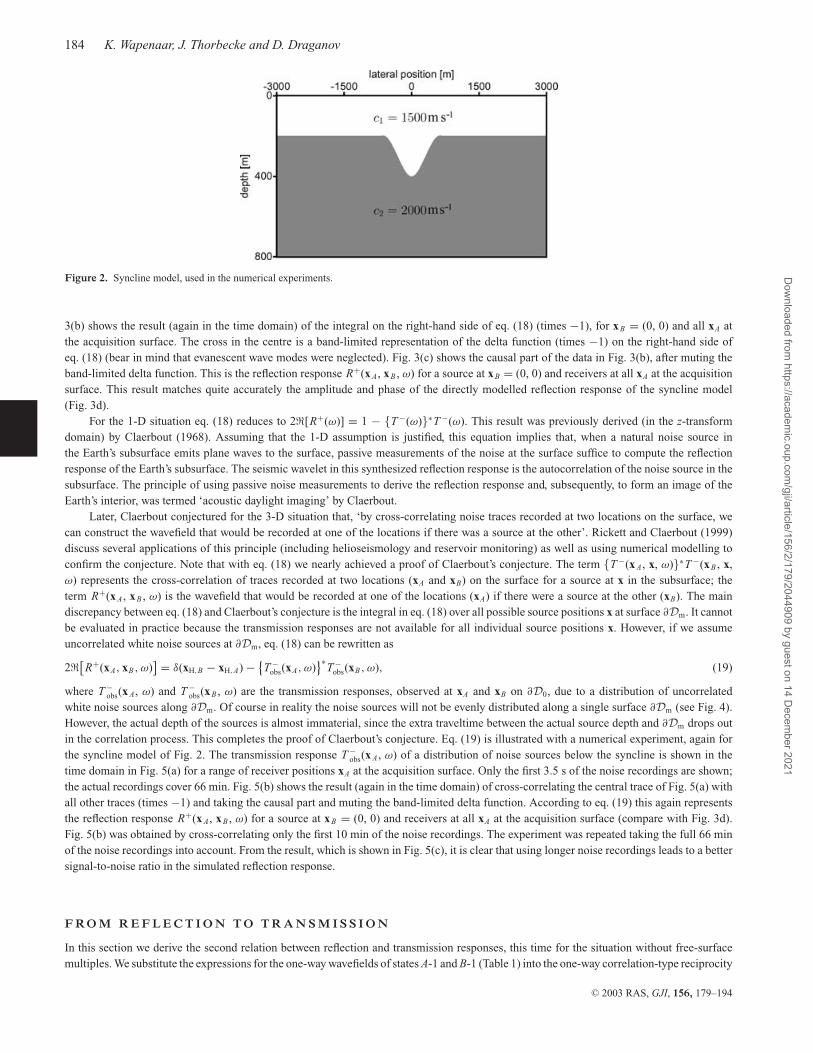
Eq. (18) is illustrated with a 2-D numerical experiment. The transmission response T −(x A, x, ω) of the syncline model in Fig. 2 isshown in the time domain in Fig. 3(a) for a fixed source at x = (0, 800) and a range of receiver positions xA at the acquisition surface. Fig.

C© 2003 RAS, GJI, 156, 179–194

Dow



ecember 2021


Figure 2. Syncline model, used in the numerical experiments.

3(b) shows the result (again in the time domain) of the integral on the right-hand side of eq. (18) (times −1), for xB = (0, 0) and all xA atthe acquisition surface. The cross in the centre is a band-limited representation of the delta function (times −1) on the right-hand side ofeq. (18) (bear in mind that evanescent wave modes were neglected). Fig. 3(c) shows the causal part of the data in Fig. 3(b), after muting theband-limited delta function. This is the reflection response R+(x A, xB , ω) for a source at xB = (0, 0) and receivers at all xA at the acquisitionsurface. This result matches quite accurately the amplitude and phase of the directly modelled reflection response of the syncline model(Fig. 3d).

For the 1-D situation eq. (18) reduces to 2�[R+(ω)] = 1 − {T −(ω)}∗T −(ω). This result was previously derived (in the z-transformdomain) by Claerbout (1968). Assuming that the 1-D assumption is justified, this equation implies that, when a natural noise source inthe Earth’s subsurface emits plane waves to the surface, passive measurements of the noise at the surface suffice to compute the reflectionresponse of the Earth’s subsurface. The seismic wavelet in this synthesized reflection response is the autocorrelation of the noise source in thesubsurface. The principle of using passive noise measurements to derive the reflection response and, subsequently, to form an image of theEarth’s interior, was termed ‘acoustic daylight imaging’ by Claerbout.

Later, Claerbout conjectured for the 3-D situation that, ‘by cross-correlating noise traces recorded at two locations on the surface, wecan construct the wavefield that would be recorded at one of the locations if there was a source at the other’. Rickett and Claerbout (1999)discuss several applications of this principle (including helioseismology and reservoir monitoring) as well as using numerical modelling toconfirm the conjecture. Note that with eq. (18) we nearly achieved a proof of Claerbout’s conjecture. The term {T −(x A, x, ω)}∗T −(xB , x,ω) represents the cross-correlation of traces recorded at two locations (xA and xB) on the surface for a source at x in the subsurface; theterm R+(x A, xB , ω) is the wavefield that would be recorded at one of the locations (xA) if there were a source at the other (xB). The maindiscrepancy between eq. (18) and Claerbout’s conjecture is the integral in eq. (18) over all possible source positions x at surface ∂Dm. It cannotbe evaluated in practice because the transmission responses are not available for all individual source positions x. However, if we assumeuncorrelated white noise sources at ∂Dm, eq. (18) can be rewritten as

2�[R+(xA, xB, ω)

] = δ(xH,B − xH,A) − {T −

obs(xA, ω)}∗

T −obs(xB, ω), (19)

where T −obs(x A, ω) and T −

obs(xB , ω) are the transmission responses, observed at xA and xB on ∂D0, due to a distribution of uncorrelatedwhite noise sources along ∂Dm. Of course in reality the noise sources will not be evenly distributed along a single surface ∂Dm (see Fig. 4).However, the actual depth of the sources is almost immaterial, since the extra traveltime between the actual source depth and ∂Dm drops outin the correlation process. This completes the proof of Claerbout’s conjecture. Eq. (19) is illustrated with a numerical experiment, again forthe syncline model of Fig. 2. The transmission response T −

obs(x A, ω) of a distribution of noise sources below the syncline is shown in thetime domain in Fig. 5(a) for a range of receiver positions xA at the acquisition surface. Only the first 3.5 s of the noise recordings are shown;the actual recordings cover 66 min. Fig. 5(b) shows the result (again in the time domain) of cross-correlating the central trace of Fig. 5(a) withall other traces (times −1) and taking the causal part and muting the band-limited delta function. According to eq. (19) this again representsthe reflection response R+(x A, xB , ω) for a source at xB = (0, 0) and receivers at all xA at the acquisition surface (compare with Fig. 3d).Fig. 5(b) was obtained by cross-correlating only the first 10 min of the noise recordings. The experiment was repeated taking the full 66 minof the noise recordings into account. From the result, which is shown in Fig. 5(c), it is clear that using longer noise recordings leads to a bettersignal-to-noise ratio in the simulated reflection response.

F RO M R E F L E C T I O N T O T R A N S M I S S I O N

In this section we derive the second relation between reflection and transmission responses, this time for the situation without free-surfacemultiples. We substitute the expressions for the one-way wavefields of states A-1 and B-1 (Table 1) into the one-way correlation-type reciprocity

C© 2003 RAS, GJI, 156, 179–194

Dow



ecember 2021


Figure 3. From transmission to reflection: illustration of eq. (18) for the 2-D medium in Fig. 2. (a) Transmission response. (b) Result of the integral on theright-hand side of eq. (18). (c) Causal part of the data in (b), after muting the band-limited delta function. This is the reflection response R+(x A , xB , ω). (d)For comparison, the directly modelled reflection response.

theorem (eq. 5). Dividing the result by s∗A(ω)sB(ω) we obtain∫

∂Dm

{T +

0 (x, xA, ω)}∗

T +0 (x, xB, ω) d2x = δ(xH,B − xH,A) −

∫∂D0

{R+

0 (x, xA, ω)}∗

R+0 (x, xB, ω) d2x, (20)

for xA and xB just above ∂D0. Note that this equation is not exact, since evanescent wave modes are neglected in the derivation of the one-waycorrelation-type reciprocity theorem. Similar expressions have been derived by Herman (1992) using the two-way reciprocity theorem (eq. 3)and by Wapenaar & Herrmann (1993) using the one-way reciprocity theorem (eq. 5). There is no unique way to resolve the transmissionresponse T +

0 (x, x A, ω) from the left-hand side of eq. (20). In Wapenaar et al. (2003) we discuss how to resolve the coda of the transmissionresponse from the left-hand side of eq. (20), given the cross-correlation of the reflection response (the right-hand side of eq. 20) for a largerange of source positions xA and xB at x3,0. Note that the inverse of the transmission coda, in combination with an inverse primary propagator,can be used in seismic reflection imaging to obtain an image in which the internal multiple scattering effects are suppressed. In this approach,the inverse primary propagator is estimated from the traveltime information in the data (as usual), whereas the inverse transmission coda is

C© 2003 RAS, GJI, 156, 179–194

Dow



ecember 2021


Figure 3. (Continued).

obtained from the cross-correlation of the reflection measurements. By way of comparison, we note that in the imaging scheme proposed byWeglein et al. (2000) the full inverse operator (primaries as well as internal multiples) is estimated directly from the reflection measurements.The advantages and disadvantages of the two methods with respect to accuracy, stability, etc. remain to be investigated.

E X P R E S S I O N S F O R F R E E - S U R FA C E M U LT I P L E S

To find a relation between the reflection responses with and without free-surface multiples, we substitute the expressions for the one-waywavefields of states A-1 and B-3 (Table 1) into the one-way convolution-type reciprocity theorem (eq. 4). Applying the source–receiverreciprocity relation (11) to the result we obtain

R+0 (xA, xB, ω) − R+(xA, xB, ω) =

∫∂D0

R+0 (xA, x, ω)R+(x, xB, ω) d2x, (21)

for xA and xB just above ∂D0. When the reflection response R+0 (x A, xB , ω) without free-surface multiples is known (for example as a

result of numerical seismic modelling), eq. (21) is an integral equation of the second kind for the reflection response R+(x A, xB , ω) with

C© 2003 RAS, GJI, 156, 179–194

Dow



ecember 2021


Figure 4. Transmission responses, observed at xA and xB, due to a distribution of uncorrelated white noise sources. According to eq. (19), their cross-correlationyields the reflection response observed at xA, as if there were an impulsive point source at xB.

free-surface multiples. On the other hand, when the response R+(x A, xB , ω) with free-surface multiples is known (from decomposed seismicmeasurements), eq. (21) is an integral equation of the second kind for the response R+

0 (x A, xB , ω) without free-surface multiples. A methodfor free-surface multiple elimination, based on a similar type of equation but derived in a different way, has been proposed by Berkhout(1982) and implemented by Verschuur et al. (1992). Fokkema & van den Berg (1993) used the two-way reciprocity theorem to derive a similarmultiple elimination scheme, which has been implemented by van Borselen et al. (1996). Eq. (21) can be seen as the ‘one-way counterpart’of the result of Fokkema & van den Berg (1993).

Next we substitute states A-2 and B-3 into eq. (4). Applying the source–receiver reciprocity relation (15) to the result we obtain

T +0 (x′

A, xB, ω) − T +(x′A, xB, ω) =

∫∂D0

T +0 (x′

A, x, ω)R+(x, xB, ω) d2x, (22)

for xB just above ∂D0 and x′A just below ∂Dm. Alternatively, substituting states A-4 and B-1 into eq. (4) and using source–receiver reciprocity

relation (16) yields

T +0 (x′

A, xB, ω) − T +(x′A, xB, ω) =

∫∂D0

T +(x′A, x, ω)R+

0 (x, xB, ω) d2x. (23)

Eqs (22) and (23) interrelate the transmission responses T +0 (x′

A, xB , ω) and T +(x′A, xB , ω) without and with free-surface multiples. Eq. (22)

can be seen as an explicit expression for the transmission response T +(x′A, xB , ω) with free-surface multiples in terms of T +

0 (x′A, x, ω) and

R+(x, xB , ω), whereas eq. (23) is an explicit expression for the transmission response T +0 (x′

A, xB , ω) without free-surface multiples in termsof T +(x′

A, x, ω) and R+0 (x, xB , ω).

S E I S M I C I N T E R F E RO M E T RY

In the previous section we substituted states A-1 and B-3 into the one-way convolution-type reciprocity theorem (eq. 4) and obtained a relationbetween reflection responses without and with free-surface multiples (eq. 21). The right-hand side of this equation contains an integral overthe product of R+

0 (x A, x, ω) and R+(x, xB , ω), which corresponds to a convolution of these terms in the time domain. Schuster (2001)proposed evaluating a similar integral over the product of {R+

0 (x A, x, ω)}∗ and R+(xB , x, ω), which corresponds to a cross-correlation inthe time domain of two reflection responses recorded at xA and xB, respectively. He showed that this leads to a new reflection responseobserved at xA, as if there was a source at xB. Note the analogy with Claerbout’s conjecture about the cross-correlation of transmissionresponses. Schuster (2001) used the term ‘seismic interferometry’ for any method that employs the cross-correlation of seismic responsesrecorded at different locations. We investigate the integral over the product of {R+

0 (x A, x, ω)}∗ and R+(xB , x, ω) by substituting states A-1and B-3 into the one-way correlation-type reciprocity theorem (eq. 5) and employing the appropriate source–receiver reciprocity relations. Weobtain

R+(xA, xB, ω) = δ(xH,B − xH,A) −∫

∂D0

{R+

0 (xA, x, ω)}∗

R+(xB, x, ω) d2x −∫

∂Dm

{T −0 (xA, x, ω)}∗T −(xB, x, ω) d2x, (24)

for xA and xB just above ∂D0. This equation shows that an integral over the correlation of reflection responses recorded at xA and xB (the firstintegral on the right-hand side along the common source coordinate x at ∂D0 of both responses) indeed contributes to the reflection responseR+(x A, xB , ω). This we call seismic reflection interferometry. It is illustrated with an example in Fig. 6, for the reflection data of Fig. 3(d).From Fig. 6(a), which represents the result of the first integral on the right-hand side of eq. (24), we observe that this seismic reflectioninterferometric result contains all events of the true reflection response R+(x A, xB , ω) (compare with Fig. 3d), but with erroneous amplitudes.

C© 2003 RAS, GJI, 156, 179–194

Dow



ecember 2021


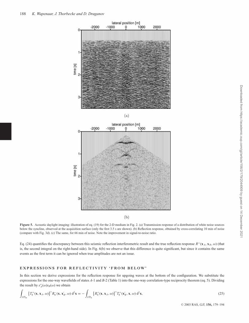
Figure 5. Acoustic daylight imaging: illustration of eq. (19) for the 2-D medium in Fig. 2. (a) Transmission response of a distribution of white noise sourcesbelow the syncline, observed at the acquisition surface (only the first 3.5 s are shown). (b) Reflection response, obtained by cross-correlating 10 min of noise(compare with Fig. 3d). (c) The same, for 66 min of noise. Note the improvement in signal-to-noise ratio.

Eq. (24) quantifies the discrepancy between this seismic reflection interferometric result and the true reflection response R+(x A, xB , ω) (thatis, the second integral on the right-hand side). In Fig. 6(b) we observe that this difference is quite significant, but since it contains the sameevents as the first term it can be ignored when true amplitudes are not an issue.

E X P R E S S I O N S F O R R E F L E C T I V I T Y ‘ F RO M B E L O W ’

In this section we derive expressions for the reflection response for upgoing waves at the bottom of the configuration. We substitute theexpressions for the one-way wavefields of states A-1 and B-2 (Table 1) into the one-way correlation-type reciprocity theorem (eq. 5). Dividingthe result by s∗

A(ω)sB(ω) we obtain∫∂Dm

{T +

0 (x, xA, ω)}∗

R−0 (x, x′

B, ω) d2x = −∫

∂D0

{R+

0 (x, xA, ω)}∗

T +0 (x′

B, x, ω) d2x, (25)

C© 2003 RAS, GJI, 156, 179–194

Dow



ecember 2021


Figure 5. (Continued.)

for xA just above ∂D0 and x′B just below ∂Dm. When the reflection response R+

0 (x, x A, ω) and the transmission response T +0 (x, x A, ω),

both without free-surface multiples, are known, eq. (25) is an integral equation of the first kind for the reflection response R−0 (x, x′

B , ω)for upgoing waves at the bottom of the configuration, just below ∂Dm, without free-surface multiples. R+

0 (x, x A, ω) could be the result offree-surface multiple elimination (eq. 21), whereas T +

0 (x, x A, ω) could be obtained from the transformation of the reflection response intothe transmission coda (eq. 20), combined with the primary transmission response. R−

0 (x, x′B , ω) can be used for imaging the configuration

between the boundaries ∂D0 and ∂Dm ‘from below’, in addition to conventional imaging ‘from above’.Next we substitute states A-3 and B-4 into eq. (5). Applying the source–receiver reciprocity relation (16) to the result, we obtain∫

∂Dm

{T +(x, xA, ω)

}∗R−(x, x′

B, ω) d2x = −T +(x′B, xA, ω), (26)

for xA at the free surface just above ∂D0 and x′B just below ∂Dm. When the transmission response T +(x, x A, ω) with free-surface multiples

is known, eq. (26) is an integral equation of the first kind for the reflection response R−(x, x′B , ω) for upgoing waves at the bottom of the

configuration, just below ∂Dm, with free-surface multiples related to the free surface just above ∂D0.Finally, by substituting states A-4 and B-4 into eq. (5), we obtain∫

∂Dm

{R−(x, x′

A, ω)}∗

R−(x, x′B, ω) d2x = δ(x′

H,B − x′H,A), (27)

for x′A and x′

B just below ∂Dm. This equation shows that the reflection response R−(x, x′A, ω) for upgoing waves at the bottom of the

configuration is unitary when there is a free surface on top of the configuration—see Fig. 1, state A-4.

C O N C L U S I O N S

We have derived a number of relations between reflection and transmission responses of 3-D inhomogeneous media. The starting point for ourderivations is given by the one-way reciprocity theorems of the convolution-type and of the correlation-type (eqs 4 and 5). These reciprocitytheorems interrelate flux-normalized downgoing and upgoing waves in two acoustic states A and B. For both reciprocity theorems the mediumbetween ∂D0 and ∂Dm is source-free and the medium parameters are assumed to be identical in both states. For all states specified in Table 1 wehave assumed that the half-space below ∂Dm is homogeneous, and that above ∂D0 there is either a free surface or a homogeneous half-space.The one-way convolution-type reciprocity theorem (eq. 4) is exact and applies to lossless as well as to dissipative media. In the derivation ofthe one-way correlation-type reciprocity theorem (eq. 5) evanescent wave modes have been ignored and the medium between ∂D0 and ∂Dm

is assumed to be lossless.We have considered reflection responses at the upper boundary ∂D0 and at the lower boundary ∂Dm as well as transmission responses

between these boundaries. All responses have been considered with and without free-surface multiples; internal multiple scattering was alwaysincluded. The mutual relations between these responses were obtained by substituting a selection of responses for the two states A and B ineither one of the reciprocity theorems (4) or (5). The assumptions discussed above apply of course also to the relations that have been derivedfrom either one of these reciprocity theorems.

C© 2003 RAS, GJI, 156, 179–194

Dow



ecember 2021


0

1

2

3

time

[s]

-2000 -1000 0 1000 2000lateral position [m]

(a)

0

1

2

3

time

[s]

-2000 -1000 0 1000 2000lateral position [m]

(b)

Figure 6. Seismic interferometry: illustration of eq. (24) for the 2-D medium in Fig. 2 and its reflection response in Fig. 3(d). (a) Result of the first integralon the right-hand side of eq. (24) (times −1). (b) Result of the second integral on the right-hand side of eq. (24) (times −1).

First we derived source–receiver reciprocity relations for the various reflection and transmission responses (eqs 11–16). Although thistype of relation is well known for full wavefields, we needed to establish them independently for the reflection and transmission responses ofdowngoing and upgoing wavefields. Since these expressions were derived from the one-way convolution-type reciprocity theorem (eq. 4) theyare exact and valid for media with or without anelastic losses. Eqs (11), (12) and (15) were previously derived in the wavenumber domain byHaines (1988).

Next we derived a relation between reflection and transmission responses including free-surface multiples (eq. 19). This is an explicitexpression for the reflection response in terms of the cross-correlation of transmission measurements. We noted that this equation confirmsClaerbout’s conjecture about acoustic daylight imaging and demonstrated this with a numerical example. We derived a second relation betweenreflection and transmission responses, this time without free-surface multiples (eq. 20). We noted that this equation can be used to derivethe transmission coda from the cross-correlation of the reflection measurements. This may be useful in seismic imaging schemes that takeinternal multiple scattering into account. Eqs (19) and (20) were derived from the one-way correlation-type reciprocity theorem (eq. 5), andhence evanescent wave modes are ignored and they are valid only for lossless media.

C© 2003 RAS, GJI, 156, 179–194

Dow



ecember 2021


We derived two classes of expressions between responses without and with free-surface multiples. The first class of expressions wasbased on the convolution-type reciprocity theorem (eq. 4) and led to the exact relations (21)–(23). Eq. (21) is similar to those employedby Berkhout (1982), Verschuur et al. (1992), Fokkema & van den Berg (1993) and van Borselen et al. (1996) for surface-related multipleelimination. The second class of expressions was based on the correlation-type reciprocity theorem (eq. 5) and led to the approximate eq. (24),which confirms one of the expressions for seismic interferometry derived by Schuster (2001).

Finally, we derived three approximate expressions (eqs 25–27) based on the correlation-type reciprocity theorem for the reflectionresponse at the lower boundary ∂Dm. These expressions may be useful for imaging ‘from below’.

Note that, because all relations apply to reflection and/or transmission responses for downgoing and/or upgoing wavefields, in practicea decomposition of measurements into downgoing and upgoing wavefields is required as a pre-processing step.

The extensions of all relations to the elastodynamic situation are discussed in Appendix A. These relations can be applied to multicom-ponent seismic data after decomposition into downgoing and upgoing P and S waves.

A C K N O W L E D G M E N T S

We thank the editors and one of the anonymous reviewers for their constructive comments. This work is supported by the Netherlands ResearchCentre for Integrated Solid Earth Science (ISES) and the Dutch Science Foundation (STW, grant DTN.4915).

R E F E R E N C E S

Berkhout, A.J., 1982. Seismic Migration. Imaging of Acoustic Energy byWavefield Extrapolation, Elsevier, Amsterdam.

Bojarski, N.N., 1983. Generalized reaction principles and reciprocity the-orems for the wave equations, and the relationship between the time-advanced and time-retarded fields, J. acoust. Soc. Am., 74, 281–285.

Chapman, C.H., 1994. Reflection/transmission coefficients reciprocities inanisotropic media, Geophys. J. Int., 116, 498–501.

Claerbout, J.F., 1968. Synthesis of a layered medium from its acoustic trans-mission response, Geophysics, 33, 264–269.

deHoop, A.T., 1988. Time-domain reciprocity theorems for acoustic wavefields in fluids with relaxation, J. acoust. Soc. Am., 84, 1877–1882.

Fokkema, J.T. & vanden Berg, P.M., 1993. Seismic Applications of AcousticReciprocity, Elsevier, Amsterdam.

Frasier, C.W., 1970. Discrete time solution of plane P- SV waves in a planelayered medium, Geophysics, 35, 197–219.

Haines, A.J., 1988. Multi-source, multi-receiver synthetic seismograms forlaterally heterogeneous media using F–K domain propagators, Geophys.J. Int., 95, 237–260.

Herman, G.C., 1992. Estimation of the inverse acoustic transmission opera-tor of a heterogeneous region directly from its reflection operator, InverseProblems, 8, 559–574.

Kennett, B. L.N., Kerry, N.J. & Woodhouse, J.H., 1978. Symmetries in thereflection and transmission of elastic waves, Geophys. J. R. astr. Soc., 52,215–230.

Kennett, B. L.N., Koketsu, K. & Haines, A.J., 1990. Propagation invariants,reflection and transmission in anisotropic, laterally heterogeneous media,Geophys. J. Int., 103, 95–101.

Koketsu, K., Kennett, B. L.N. & Takenaka, H., 1991. 2-D reflectivity methodand synthetic seismograms for irregularly layered structures—II. Invariantembedding approach, Geophys. J. Int., 105, 119–130.

Osen, A., Amundsen, L. & Reitan, A., 1996. Multiple attenuation on mul-ticomponent sea floor data, in 58th Mtg, Eur. Assoc. Explor. Geophys.,Extended Abstracts. Abstract No. B024, ed. Feenstra, D.J., Eur. Assoc.Explor. Geophys., Houten, the Netherlands.

Rickett, J. & Claerbout, J.F., 1999. Acoustic daylight imaging via spectral

factorization: helioseismology and reservoir monitoring in ed. Ross, C.P.,69th Ann. Int. Mtg, Soc. Explor. Geophys., Expanded Abstracts, pp. 1675–1678. Soc. Explor. Geophys., Tulsa, OK, USA.

Schalkwijk, K.M., Wapenaar, C.P.A. & Verschuur, D.J., 1998. Decomposi-tion of multicomponent ocean-bottom data in two steps, in eds Brown,R. & Comeaux, L., 68th Ann. Int. Mtg, Soc. Explor. Geophys., ExpandedAbstracts, pp. 1425–1428. Soc. Explor. Geophys., Tulsa, OK, USA.

Schuster, G.T., 2001. Theory of daylight/interferometric imaging: tutorial,63rd Mtg, Eur. Assoc. Explor. Geophys., Extended Abstracts. AbstractNo. A032, ed. Nordberg, H., Eur Assoc. Explor. Geophys., Houten, theNetherlands.

Takenaka, H., Kennett, B.L.N. & Koketsu, K., 1993. The integral operatorrepresentation of propagation invariants for elastic waves in irregularlylayered media, Wave Motion, 17, 299–317.

Ursin, B., 1983. Review of elastic and electromagnetic wave propagation inhorizontally layered media, Geophysics, 48, 1063–1081.

van Borselen, R.G., Fokkema, J.T. & vanden Berg, P.M., 1996. Surface-related multiple elimination, Geophysics, 61, 202–210.

Verschuur, D.J., Berkhout, A.J. & Wapenaar, C.P.A., 1992. Adaptive surface-related multiple elimination, Geophysics, 57, 1166–1177.

Wapenaar, C.P.A. & Grimbergen, J.L.T., 1996. Reciprocity theorems forone-way wave fields, Geophys. J. Int., 127, 169–177.

Wapenaar, C. P.A. & Herrmann, F.J., 1993. True amplitude migration takingfine-layering into account, 63rd Ann. Int. Mtg, Soc. Explor. Geophys., Ex-panded Abstracts, pp. 653–656. Soc. Explor. Geophys., Tulsa, OK, USA.

Wapenaar, C.P.A., Herrmann, P., Verschuur, D.J. & Berkhout, A.J., 1990. De-composition of multicomponent seismic data into primary P- and S-waveresponses, Geophys. Prospect., 38, 633–662.

Wapenaar, C. P.A., Draganov, D. & Thorbecke, J.W., 2003. Relations be-tween codas in reflection and transmission data and their applications inseismic imaging, in ed. Uchida, T., 6th Ann. Int. Mtg, Soc. Explor. Geo-phys. of Japan, Expanded Abstracts, pp. 152–159. Soc. Explor. Geophys.of Japan, Tokyo, Japan..

Weglein, A.B., Matson, K.H., Foster, D.J., Carvalho, P.M., Corrigan, D. &Shaw, S.A., 2000. Imaging and inversion at depth without a velocitymodel: theory, concepts and initial evaluation, in ed. Cary, P., 70th Ann.Int. Mtg, Soc. Explor. Geophys., Expanded Abstracts, pp. 1016–1019. Soc.Explor. Geophys., Tulsa, OK, USA.

A P P E N D I X A : E X T E N S I O N T O T H E E L A S T O DY N A M I C S I T UAT I O N

To derive relations between reflection and transmission responses for elastodynamic waves in 3-D inhomogeneous elastic media, we haveagain the choice between reciprocity theorems for two-way and one-way wavefields. In the former case the reciprocity theorems are formulatedin terms of particle velocities and stresses in two states (similarly to the propagation invariant introduced by Kennett et al. 1990); in the lattercase they are formulated in terms of flux-normalized downgoing and upgoing P and S waves in both states. Hence, elastodynamic two-wayreciprocity theorems can be applied directly to observable quantities, such as the three components of particle velocity measured by geophonesin multi-component seismic data acquisition. However, similarly to in the acoustic case, elastodynamic reflection and transmission responses

C© 2003 RAS, GJI, 156, 179–194

Dow



ecember 2021


are transfer functions between downgoing and upgoing P and S waves. For this reason the elastodynamic one-way reciprocity theorems arepreferred as the starting point for deriving the relations between the various reflection and transmission responses. To apply the results inpractice, the multi-component data should be decomposed into downgoing and upgoing P and S waves as a pre-processing step (Wapenaaret al. 1990; Osen et al. 1996; Schalkwijk et al. 1998).

In the following we discuss the extensions of all results derived for the acoustic situation to the elastodynamic situation.

Elastodynamic one-way reciprocity theorems

For the elastodynamic situation, the one-way reciprocity theorems (4) and (5) are replaced by∫∂D0

{(P+

A )tP−B − (P−

A )tP+B

}d2x =

∫∂Dm

{(P+

A )tP−B − (P−

A )tP+B

}d2x (A1)

and∫∂D0

{(P+

A )†P+B − (P−

A )†P−B

}d2x =

∫∂Dm

{(P+

A )†P+B − (P−

A )†P−B

}d2x, (A2)

respectively, where ‘t’ denotes transposition and ‘†’ denotes transposition and complex conjugation. The one-way wavefield vectors are definedas follows

P±A =

±A

�±A

ϒ±A

, P±

B =

±B

�±B

ϒ±B

, (A3)

where ±, �± and ϒ± represent the flux-normalized downgoing and upgoing P, S1 and S2 waves, respectively, for states A and B (Wapenaar& Grimbergen 1996).

Specification of the states for the one-way reciprocity theorems

In Table 1 the scalar acoustic one-way wavefields P±A need to be replaced by the vector elastodynamic one-way wavefields P±

A . Furthermore,the scalar reflection and transmission responses R±

0 , R±, T ±0 and T± have to be replaced by 3 × 3 matrices R±

0 , R±, T±0 and T±, respectively,

which have the following form

R±(x, xA, ω) =

R±φ,φ R±

φ,ψ R±φ,υ

R±ψ,φ R±

ψ,ψ R±ψ,υ

R±υ,φ R±

υ,ψ R±υ,υ

(x, xA, ω), (A4)

etc., where R±β,α(x, x A, ω) denotes the reflection response in terms of an incident α-wavefield at xA and a reflected β-wavefield at x. The

scalar free-surface reflection coefficient r− in Table 1 (with r− = −1) should be replaced by a 3 × 3 operator matrix r̂−, where the circumflexdenotes a pseudo-differential operator acting on the x1- and x2-coordinates. In Appendix B we show that r̂− obeys the following properties

{r̂−}t = r̂−, (A5)

{r̂−}† r̂− = I, (A6)

where I is the 3 × 3 identity matrix. Finally, in Table 1 we should replace δ(xH − xH,A) by Iδ(xH − xH,A), sA(ω) by s A(ω) (a 3 × 1 vectorrepresenting source spectra for the various wave types) and 0 by 0 (the 3 × 1 null vector). Similar replacements should be made for state B.

Source–receiver reciprocity

Substituting the expressions for the elastodynamic one-way wavefields of states A-1 and B-1 of the modified Table 1 into the one-wayconvolution-type reciprocity theorem (eq. A1) we obtain∫

∂D0

stA(ω)

[δ(xH − xH,A)R+

0 (xH, x3,0, xB, ω) − {R+

0 (xH, x3,0, xA, ω)}t

δ(xH − xH,B)]sB(ω) d2x = 0. (A7)

Since this expression should hold for any sA(ω) and sB(ω), we obtain

R+0 (xA, xB, ω) = {

R+0 (xB, xA, ω)

}t, (A8)

for xA and xB just above ∂D0. This is the elastodynamic equivalent of the source–receiver reciprocity relation (11). In a similar way we findthe elastodynamic equivalents of the source–receiver reciprocity relations (12)–(16):

R−0 (x′

A, x′B, ω) = {R−

0 (x′B, x′

A, ω)}t, (A9)

R+(xA, xB, ω) = {R+(xB, xA, ω)

}t, (A10)

R−(x′A, x′

B, ω) = {R−(x′

B, x′A, ω)

}t, (A11)

C© 2003 RAS, GJI, 156, 179–194

Dow



ecember 2021


T+0 (x′

A, xB, ω) = {T−0 (xB, x′

A, ω)}t, (A12)

T+(x′A, xB, ω) = {T−(xB, x′

A, ω)}t, (A13)

for xA and xB just above ∂D0 and x′A and x′

B just below ∂Dm. Eqs (A8), (A9) and (A12) were previously derived in the wavenumber domain byKennett et al. (1990). Note that we made use of the first symmetry property of the free-surface reflection operator r̂− (eq. A5) in the derivationof eqs (A10), (A11) and (A13).

Using the form introduced in eq. (A4) we obtain for example from eq. (A10) that

R+α,β (xA, xB, ω) = R+

β,α(xB, xA, ω). (A14)

This equation states that the upgoing α-wavefield at xA due to a downgoing β-wavefield at xB is identical to the upgoing β-wavefield at xB

due to a downgoing α-wavefield at xA.

From transmission to reflection

Using the second symmetry property of the free-surface reflection operator r̂− (eq. A6), we find for the elastodynamic version of the relationbetween reflection and transmission responses with free-surface multiples, analogous to eq. (18),

−r̂−(xA)R+(xA, xB, ω) − {R+(xA, xB, ω)}∗{r̂−(xB)}† = Iδ(xH,B − xH,A) −∫

∂Dm

{T−(xA, x, ω)}∗{T−(xB, x, ω)}t d2x, (A15)

for xA and xB at the free surface, just above ∂D0. This equation is the basis for resolving the P and S reflection responses from the cross-correlation of the P and S transmission responses and finds its application in acoustic daylight imaging.

From reflection to transmission

Analogous to the acoustic relation (eq. 20) between reflection and transmission responses without free-surface multiples, we obtain for theelastodynamic situation∫

∂Dm

{T+

0 (x, xA, ω)}†

T+0 (x, xB, ω) d2x = Iδ(xH,B − xH,A) −

∫∂D0

{R+

0 (x, xA, ω)}†

R+0 (x, xB, ω) d2x, (A16)

for xA and xB just above ∂D0. This equation is the basis for resolving the P and S wave transmission codas from the cross-correlation of theP and S reflection responses. These transmission codas may be used to derive inverse propagators that take internal multiple scattering intoaccount in elastodynamic seismic imaging.

Expressions for free-surface multiples

The elastodynamic equivalent of the acoustic relation between reflection responses with and without free-surface multiples (eq. 21) reads

R+0 (xA, xB, ω) − R+(xA, xB, ω) = −

∫∂D0

R+0 (xA, x, ω)r̂−R+(x, xB, ω) d2x, (A17)

for xA and xB just above ∂D0. A similar relation was obtained previously by Wapenaar et al. (1990) and illustrated with a numerical example,demonstrating its application in elastodynamic multiple elimination of decomposed multi-component data in a 2-D inhomogeneous elasticmedium.

The elastodynamic equivalents of eqs (22) and (23) read

T+0 (x′

A, xB, ω) − T+(x′A, xB, ω) = −

∫∂D0

T+0 (x′

A, x, ω)r̂−R+(x, xB, ω) d2x (A18)

and

T+0 (x′

A, xB, ω) − T+(x′A, xB, ω) = −

∫∂D0

T+(x′A, x, ω)r̂−R+

0 (x, xB, ω) d2x, (A19)

for xB just above ∂D0 and x′A just below ∂Dm.

Seismic interferometry

Analogous to eq. (24) we obtain

−r̂−(xA)R+(xA, xB, ω) = Iδ(xH,B − xH,A) −∫

∂D0

{R+

0 (xA, x, ω)}∗{R+(xB, x, ω)}t d2x

−∫

∂Dm

{T−

0 (xA, x, ω)}∗{T−(xB, x, ω)}t d2x, (A20)

for xA and xB just above ∂D0. This equation is the basis for elastodynamic seismic interferometry.

C© 2003 RAS, GJI, 156, 179–194

Dow



ecember 2021


Expressions for reflectivity ‘from below’

Finally, the elastodynamic equivalents of the expressions for reflectivity ‘from below’ (eqs 25, 26 and 27) read∫∂Dm

{T+

0 (x, xA, ω)}†

R−0 (x, x′

B, ω) d2x = −∫

∂D0

{R+

0 (x, xA, ω)}†

T+0 (x′

B, x, ω) d2x, (A21)

for xA just above ∂D0 and x′B just below ∂Dm;∫

∂Dm

{T+(x, xA, ω)

}†R−(x, x′

B, ω) d2x = r̂−(xA)T+(x′B, xA, ω), (A22)

for xA at the free surface just above ∂D0 and x′B just below ∂Dm; and∫

∂Dm

{R−(x, x′A, ω)}†R−(x, x′

B, ω) d2x = Iδ(x′H,B − x′

H,A), (A23)

for x′A and x′

B just below ∂Dm. These expressions are the basis for elastodynamic imaging of the configuration between the boundaries ∂D0

and ∂Dm ‘from below’, in addition to elastodynamic imaging ‘from above’.

A P P E N D I X B : T H E F R E E - S U R F A C E R E F L E C T I O N O P E R A T O R

For the derivation of the properties of the free-surface reflection operator r̂− we choose ∂D0 again at x 3,0 + ε, that is, just below the freesurface, but the other integration boundary is chosen above the free surface. Since no wavefields are present in the upper half-space, theintegral over this upper boundary is zero. Hence, if we choose the sources for the one-way wavefields below ∂D0, the elastodynamic one-wayreciprocity theorems read∫

∂D0

{(P+

A )tP−B − (P−

A )tP+B

}d2x = 0 (B1)

and∫∂D0

{(P+A )†P+

B − (P−A )†P−

B } d2x = 0. (B2)

The free-surface reflection operator r̂− transforms an upgoing elastodynamic wavefield at ∂D0 (that is, just below the free surface) into adowngoing wavefield at ∂D0. Hence, for states A and B we have

P+A (x, ω) = r̂−P−

A (x, ω), (B3)

P+B (x, ω) = r̂−P−

B (x, ω), (B4)

for x at ∂D0. Substitution into eqs (B1) and (B2) gives∫∂D0

{P−A (x, ω)}t({r̂−}t − r̂−)P−

B (x, ω) d2x = 0 (B5)

and∫∂D0

{P−A (x, ω)}†({r̂−}† r̂− − I)P−

B (x, ω) d2x = 0, (B6)

respectively, where {r̂−}t and {r̂−}† denote the transposed and adjoint free-surface reflection operators, respectively. Since eqs (B5) and (B6)should hold for any P−

A (x, ω) and P−B (x, ω), we obtain

{r̂−}t = r̂−, (B7)

{r̂−}† r̂− = I. (B8)

C© 2003 RAS, GJI, 156, 179–194

Dow



ecember 2021

relations between reflection and transmission responses of three

Documents