relating measurement patterns to circuits via pauli flow
TRANSCRIPT
M. Backens, C. Heunen (Eds.): Quantum Physics and Logic (QPL) 2021
EPTCS 343, 2021, pp. 50–101, doi:10.4204/EPTCS.343.4
Relating Measurement Patterns to Circuits via Pauli Flow
Will Simmons
Cambridge Quantum Computing Ltd9a Bridge Street, Cambridge, UK
Department of Computer Science, University of OxfordWolfson Building, Parks Road, Oxford, UK
The one-way model of Measurement-Based Quantum Computing and the gate-based circuit model
give two different presentations of how quantum computation can be performed. There are known
methods for converting any gate-based quantum circuit into a one-way computation, whereas the
reverse is only efficient given some constraints on the structure of the measurement pattern. Causal
flow and generalised flow have already been shown as sufficient, with efficient algorithms for identi-
fying these properties and performing the circuit extraction. Pauli flow is a weaker set of conditions
that extends generalised flow to use the knowledge that some vertices are measured in a Pauli basis.
In this paper, we show that Pauli flow can similarly be identified efficiently and that any measurement
pattern whose underlying graph admits a Pauli flow can be efficiently transformed into a gate-based
circuit without using ancilla qubits. We then use this relationship to derive simulation results for the
effects of graph-theoretic rewrites in the ZX-calculus using a more circuit-like data structure we call
the Pauli Dependency DAG.
1 Introduction
There are numerous approaches to quantum computation that differ in how problems are encoded and
how the system evolves over time. The one-way model [31] is a variant of Measurement-Based Quantum
Computing (MBQC) where the inputs are embedded into a general graph state, and the chosen computa-
tion is specified by a sequence of single-qubit measurements to apply, consuming the state and inducing
a desired output state on the remaining qubits. In contrast, the gate-based model [29] applies unitary
gates from some universal gateset to the input qubits directly. Gate-based circuits may use ancilla qubits
and measurements, though they are only necessary for expanding to a larger state space for outputs and
reading out final data.
There is a wide literature on rewriting both measurement patterns [16, 17, 32] and circuits [2, 11, 18,
21,25,34] to reduce the resource cost. Of particular interest here is the use of graph-theoretic rewrites of
ZX-diagrams (in close correspondence with measurement patterns [16]) by Kissinger and van de Weter-
ing [21], and of representations focussed on sequences of rotations about Pauli tensors such as by Zhang
and Chen [34] herein referred to as Pauli Dependency DAGs (PDDAGs) as they capture the temporal de-
pendencies between these rotations. Both works presented these as techniques for T gate reduction with
identical performance. The extraction method in this paper maps a measurement pattern/ZX-diagram
directly into the form of a PDDAG, allowing us to formally demonstrate that each of the graph-theoretic
rewrites can be simulated by moving Clifford-angled rotations through the PDDAG. This complements
existing work on deriving equivalences between the PathSum formalism and the ZH calculus [3,4,23] and
between different graphical calculi [22,28] which have shown to provide useful insight on the semantics
of operations for the more abstract calculi.

W. Simmons 51
Previous work in this area has given algorithms for extracting circuits from measurement patterns
that satisfy flow properties which describe how the errors from unwanted measurement outcomes can
be corrected using the stabilizers of the graph state [5, 7]. The weakest such property that allows for
interesting (i.e. non-Pauli) measurements is generalised flow (gflow) for which the single-plane form
exactly describes the set of patterns that are uniformly, strongly, and stepwise deterministic [9]. Pauli
flow [9] weakens the uniformity condition by labelling some of the measurements as being in a Pauli
basis rather than at some arbitrary angle in a plane of the Bloch sphere. This allows for more interesting
corrections that make use of Pauli projections to absorb some terms of the graph state stabilizers. This
paper directly extends the works of Mhalla and Perdrix [27] and Backens et al. [5] for gflow to handle
this wider class of measurement patterns.
This paper starts by laying out the key definitions and concepts behind measurement patterns and
existing results on causal flow and gflow in Section 2. Section 3 will give a short overview of the Pauli
Dependency DAG structure and how it can be used to rewrite circuits. We will then introduce the notion
of Pauli flow and decompose the circuit extraction problem to generate a procedure that works for any
measurement pattern with Pauli flow in Section 4. Then Section 5 will cover a number of methods of
rewriting measurement patterns in turn and investigate their effects on the PDDAG extracted to show
how they can be simulated.
2 Measurement-Based Quantum Computing
The one-way model follows the typical structure of MBQC of building some resource state which is then
consumed by single-qubit measurements. The particular resource considered is a graph state, constructed
by matching qubits (inputs and ancillas prepared in the |+〉 = 1√2(|0〉+ |1〉) state) with vertices in a
graph, and entangling them (with a CZ gate) according to the edges. Measurements are generally non-
deterministic so, in order to have a deterministic effect overall, local gates can be applied to the remaining
qubits to counteract the difference between the projectors for each outcome, giving the net effect of post-
selecting the desired outcome. The introduction of such correction gates can be viewed as adapting the
choice of basis for the future measurements.
Single qubit measurements are characterised by the bases they project into, which themselves can
be described by a vector in the Bloch sphere. For MBQC, we conventionally restrict measurements into
a plane of the Bloch sphere spanned by two of the Pauli bases. Such planar measurement bases are
described by the following for α ∈ [0,2π):
|+XY,α〉= 1√2
(
|0〉+ eiα |1〉)
|−XY,α〉= 1√2
(
|0〉− eiα |1〉)
|+XZ,α〉= cos(
α2
)
|0〉+ sin(
α2
)
|1〉 |−XZ,α〉= sin(
α2
)
|0〉− cos(
α2
)
|1〉 (1)
|+YZ,α〉= cos(
α2
)
|0〉+ isin(
α2
)
|1〉 |−YZ,α〉= sin(
α2
)
|0〉− icos(
α2
)
|1〉with the following special cases for Pauli measurements for α = aπ (a ∈ {0,1}):
|+X ,aπ〉= 1√2(|0〉+(−1)a |1〉) |−X ,aπ〉= 1√
2(|0〉− (−1)a |1〉)
|+Y,aπ〉= 1√2(|0〉+ i(−1)a |1〉) |−Y,aπ〉= 1√
2(|0〉− i(−1)a |1〉) (2)
|+Z,aπ〉= (1−a) |0〉+a |1〉 |−Z,aπ〉= a |0〉+(1−a) |1〉For any measurement basis, the negative outcome at angle α is equivalent to the positive outcome at
angle α +π . We usually treat the positive measurement outcome as the desired branch, i.e. the projector
we want to apply to achieve our desired end state.
52 Relating Measurement Patterns to Circuits via Pauli Flow
Formally, measurement patterns (i.e. MBQC programs) are defined as follows:
Definition 2.1 (Measurement pattern). A measurement pattern consists of a collection V of qubits with
distinguished subsets I,O ⊆V of inputs and outputs, and a sequence of commands from:
• Preparations Nu, initialising qubit u /∈ I to |+〉;• Entangling operators Euv, applying a CZ gate between distinct qubits u,v ∈V ;
• Destructive measurements Mλ ,αu , projecting qubit u /∈ O onto either |+λ ,α〉 with outcome 0 or
|−λ ,α〉 with outcome 1;
• Corrections [Xu]v or [Zu]
v, conditionally applying an X gate or a Z gate to qubit u∈V if the outcome
of the measurement for qubit v was 1.
A measurement pattern is runnable if additionally:
• All non-input qubits are prepared exactly once;
• A non-input qubit is not acted on by any other command before its preparation;
• All non-output qubits are measured exactly once;
• A non-output qubit is not acted on by any other command after its measurement;
• No correction depends on an outcome not yet measured.
The intended branch of a measurement pattern (where all measurement outcomes are 0 and hence no
corrections are required) can be summarised by a tuple (Γ,α) of a labelled open graph Γ describing the
entanglement and measurement planes, and an assignment of measurement angles α : O → [0,2π).
Definition 2.2 (Labelled open graph). A labelled open graph is a tuple Γ = (G, I,O,λ ) where G = (V,E)is an undirected graph, I,O ⊆ V are (possibly overlapping) subsets of vertices for inputs and outputs
respectively, and λ : O →{XY,XZ,YZ,X ,Y,Z} is a labelling function assigning a measurement plane or
Pauli to each non-output vertex.
Remark 2.3. To fix notation, we will use I =V \ I for non-input (prepared) vertices and O =V \O for
non-output (measured) vertices. u ∼ v denotes vertices u,v ∈ V being adjacent in G. Neighbour sets
are NG(u) := {w ∈ V |w ∼ u} and odd neighbourhoods are OddG(A) := {w ∈V | |NG(w)∩A| is odd},
writing Odd(A) when the choice of graph is obvious. The symmetric difference of sets is written as
A∆B := (A\B)∪(B\A). When drawing diagrams for measurement patterns, we will distinguish between
measured and output vertices as filled and unfilled points respectively, and inputs are specified by boxes
around the vertices. For linear maps, subscripts may be used to specify that a map acts on some given
qubit(s) and is the identity on all others, such as 〈+λ(v),α(v)|v or Pv for some Pauli P.
Each branch (combination of measurement outcomes) gives rise to a linear map from the inputs to
the outputs based on the commands run and the projections observed. The overall channel from con-
sidering all branches is a completely-positive trace-preserving map whose Kraus maps are exactly the
branch maps. When we have a strongly deterministic pattern (all branches are equal up to global phase),
we just associate it with the linear map of the intended branch. Since runnable patterns can be standard-
ised to perform all initialisations first, then all entangling gates, and finally alternate measurements and
corrections, this linear map also has a standard representation.
Definition 2.4 (Linear map of a pattern). The linear map associated with a measurement pattern (Γ,α)is given by
MΓ,α :=
(
∏u∈O
〈+λ(u),α(u)|u
)
EGNI (3)

W. Simmons 53
where EG := ∏u∼v Euv entangles pairs of adjacent qubits in the graph with CZ gates and NI := ∏u∈I Nu
initialises every non-input in the |+〉 state.
Interpreting the graph state as EGNI gives rise to a stabilizer per initialised vertex u ∈ I:
EGNI = EGXuNI =
(
∏v∈NG(u)
Zv
)
XuEGNI (4)
Since the linear map of a pattern is not just a simple graph state but a projected graph state, it is
possible for some Pauli terms introduced by graph state stabilizers to be absorbed by the Pauli projections:
〈+X ,aπ |u = (−1)a 〈+X ,aπ |u Xu
〈+Y,aπ |u = (−1)a 〈+Y,aπ |uYu
〈+Z,aπ |u = (−1)a 〈+Z,aπ |u Zu
(5)
These stabilizers and Pauli absorptions are practical for deriving possible means of correcting for
unwanted measurement outcomes.
The intention behind different types of flow conditions is to capture the ability to propagate errors
from unwanted measurement outcomes forward to the rest of the circuit in order to correct them, aiming
for stepwise determinism (each measurement can be corrected independently). Causal flow is the sim-
plest case where we suppose all vertices are measured in the XY basis and each error can be corrected by
considering a single stabilizer of the graph state.
Definition 2.5 (Causal flow [13]). Given a labelled open graph Γ = (G, I,O,λ ) such that ∀u ∈ O.λ (u) =XY , a causal flow for Γ is a tuple ( f ,≺) of a map f : O → I and a strict partial order ≺ over V such that
for all v ∈ O:
• v ∼ f (v)
• v ≺ f (v)
• ∀w ∈ NG( f (v)).w = v∨ v ≺ w
The idea here is that Zv from the graph stabilizer(
∏w∈NG( f (v)) Zw
)
X f (v) will eliminate the effect of the
measurement error on qubit v, meaning we can correct the error by applying(
∏w∈NG( f (v))\{v} Zw
)
X f (v)
and implicitly invoking the stabilizer. The partial order ≺ indicates a required order of the measurements,
ensuring that none of the vertices required for correcting v have been measured yet.
Generalised flow takes a similar approach, but allows us to take combinations of the basic stabilizers.
If the stabilizer of a candidate f (v) would require a Z correction on some u ∈ NG( f (v)) that has already
been measured, there may exist some other stabilizer we can apply that cancels out the Z for us. Now,
instead of the stabilizer being determined by a single vertex f (v) ∈ I, we have a set g(v) ⊆ I giving(
∏w∈Odd(g(v)) Zw
)(
∏w∈g(v) Xw
)
up to phase. By relaxing these restrictions on the stabilizers used, we can
also generate Y or X on the measured vertex, allowing the correction of measurements in the XZ and Y Z
planes respectively.
Definition 2.6 (Generalised flow [9]). Given a labelled open graph Γ = (G, I,O,λ ) such that ∀u ∈O.λ (u) ∈ {XY,XZ,YZ}, a generalised flow (or gflow) for Γ is a tuple (g,≺) of a map g : O → P[I]and a strict partial order ≺ over V such that for all v ∈ O:
• ∀w ∈ g(v).v 6= w ⇒ v ≺ w
• ∀w ∈ Odd(g(v)).v 6= w ⇒ v ≺ w

54 Relating Measurement Patterns to Circuits via Pauli Flow
Gate Equivalent Pauli exponentials
CXct e−i
π4
ZcXt eiπ4
Zceiπ4
Xt
CZct e−i
π4
ZcZt eiπ4
Zceiπ4
Zt
RZ(α) e−i
α2
Z
RX(α) e−i
α2
X
H e−i
π4
Ze−i
π4
Xe−i
π4
Z
CCXabt e−i
π8
ZaZbXt eiπ8
ZaZbeiπ8
ZaXt eiπ8
ZbXt e−i
π8
Za e−i
π8
Zbe−i
π8
Xt
Table 1: Summary of conversions from common gates into Pauli exponentials (up to global phase). Sub-
scripts are used to indicate specific qubits for multi-qubit gates. Other gates can similarly be represented
by first decomposing into a universal gate set such as {CX ,RZ,RX} and optionally tidying up using the
Reorder Rules.
• λ (v) = XY ⇒ v /∈ g(v)∧ v ∈ Odd(g(v))
• λ (v) = XZ ⇒ v ∈ g(v)∧ v ∈ Odd(g(v))
• λ (v) = Y Z ⇒ v ∈ g(v)∧ v /∈ Odd(g(v))
There exist polynomial-time algorithms for identifying whether or not a labelled open graph admits
causal flow or gflow [5, 14, 27], and for extracting an equivalent unitary circuit for the measurement
pattern given either type of flow [5, 7].
3 Pauli Dependency DAGs
The Pauli Dependency DAG is a data structure for representing the action of a pure quantum circuit that
abstracts away gate set, Clifford gates, and gate commutations. This was notably covered in the work
of Zhang and Chen [34] where it was used to identify possible pairs of T gates which could be merged
through some sequence of gate commutations and Clifford gate relations in order to reduce the number
of T gates in the circuit. Similar structures are also covered by Litinski [24] for compiling circuits for
lattice surgery and by Gosset et al. [19] as an intermediate for synthesis of Clifford+T circuits.
The Clifford group is the group of linear maps that can be formed from CX , Hadamard, and RZ(π2)
with qubit initialisation in the |0〉 state. These hold a special place in quantum theory as the maximal
group of actions under which the Pauli group is closed. Their behaviour is conveniently captured by the
stabilizer framework, allowing for canonical representations like the stabilizer tableau [1, 33]. They are
often viewed as the “easy” gates in a circuit because of their simple algebra, efficient simulation [1, 20],
and low resource cost in many error correction schemes [10].
Most common gate types can be expressed as (combinations of) Pauli exponentials (eiθ P for some
P ∈ {I,X ,Y,Z}⊗n), which also benefit from elegant relations with stabilizers.
Lemma 3.1 (Product Rotation Lemma). Let A and B be commuting operators such that BC = C for
some linear map C . Then eiθ AC = eiθ ABC .
Proof. For any analytic function F(A), we can expand its Taylor series in F(A)C , then introduce and
commute B in each term to form the Taylor series for F(AB)C .

W. Simmons 55
Pauli exponentials where the coefficient is an integral multiple of π4
correspond to Clifford gates.
The action of Clifford gates on both Paulis and arbitrary Pauli exponentials can be summarised in a few
equations.
Lemma 3.2 (Reorder Rules). For any Pauli strings A,B ∈ {I,X ,Y,Z}⊗n and angles θ ,φ , if A and B
commute, then
eiθ AB = Beiθ A (6)
eiθ AeiφB = eiφBeiθ A (7)
and otherwise (i.e. they anticommute)
eiπ4
AB = (iAB)ei
π4
A (8)
eiπ4
AeiφB = eiφ(iAB)e
iπ4
A (9)
Proof. Any operator satisfying A2 = I and real θ permit the decomposition eiθ A = cosθ I + isin θA by
grouping terms in the Taylor expansion. Each equation follows from decomposing one of the exponen-
tials in this way. Whilst the right-hand side of Equation 9 appears to contain a real exponent, remember
that iAB is a real Pauli string when A and B anticommute.
We can represent any circuit as a set of qubit initialisations followed by a sequence of Pauli exponen-
tials by decomposing each gate in turn. The above rules can then be used to move any Clifford-angled
exponentials to the start of the circuit, resulting in the product form(
∏k eiφkAk)
C where C is a stabilizer
process and each φk is not an integral multiple of π4
. Previous presentations [24,34] collected the Clifford
gates at the end of the circuit rather than at the start. When considering unitary circuits, the choice of
direction is arbitrary, but in the general case we may not always be able to transport qubit initialisations
through the Pauli exponentials to the end.
C can be expressed canonically by its stabilizer tableau. Specifically, since we could have an arbitrary
number of inputs we need a variant mixing the extremes of the unitary case [1] and the usual state
case [33] to capture both how Paulis over the inputs are transformed to Pauli strings over the outputs
and additional generators for free stabilizers over the outputs. In examples, we will describe this by the
stabilizers of the Choi operator of C (which we shall refer to as an isometry tableau for clarity), from
which it is simple to convert it to any binary matrix format of choice. Such tableaux can be identified and
synthesised by embedding them into unitary tableaux by breaking down the isometry into an initialisation
of |O|− |I| qubits in the |0〉 state followed by a unitary circuit which maps Z on the initialised qubits to
each of the free output stabilizers and X to any choice of operators that extend our generators to span the
full Pauli group. Since the rows are just generators for the stabilizer group, we still have the notion of
“free actions” given by reordering rows or multiplying two rows together.
For the rotation list, there is still some obvious redundancy in the product form resulting from com-
mutations. Because anticommuting Pauli strings prevent commutation of their exponentials, any valid
ordering of the rotations will preserve the relative order of rotations with anticommuting strings, induc-
ing a temporal dependency between them. Taking the transitive closure of these dependencies gives a
partial order between the exponentials which represents ∏k eiφkAk up to any number of commutations.
Definition 3.3 (Pauli Dependency DAG). A Pauli Dependency DAG (PDDAG) for a circuit is a pair
of an isometry tableau for a Clifford map C and a directed acyclic graph for a partial order ≺ over
56 Relating Measurement Patterns to Circuits via Pauli Flow
S RY (α3)
RX(α4)
RY (α5) RZ(α6)RZ(α0) RY (α2)
RZ(α1) RY (α7)
Ins Outs Sign
X Y +X X +
Z Z +Z Z +
(Z1I2,−α0) (X1I2,α2) (Y1X2,−α3) (Z1I2,−α6)
(Y1X2,−α5)
(I1Z2,−α1) (I1X2,α4) (I1Y2,−α7)
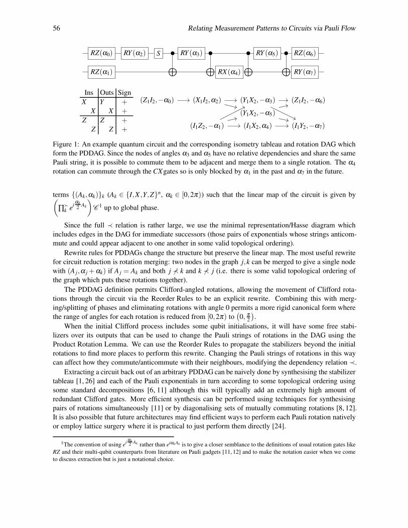
Figure 1: An example quantum circuit and the corresponding isometry tableau and rotation DAG which
form the PDDAG. Since the nodes of angles α3 and α5 have no relative dependencies and share the same
Pauli string, it is possible to commute them to be adjacent and merge them to a single rotation. The α4
rotation can commute through the CXgates so is only blocked by α1 in the past and α7 in the future.
terms {(Ak,αk)}k (Ak ∈ {I,X ,Y,Z}n, αk ∈ [0,2π)) such that the linear map of the circuit is given by(
∏≻k e
iαk
2Ak
)
C 1 up to global phase.
Since the full ≺ relation is rather large, we use the minimal representation/Hasse diagram which
includes edges in the DAG for immediate successors (those pairs of exponentials whose strings anticom-
mute and could appear adjacent to one another in some valid topological ordering).
Rewrite rules for PDDAGs change the structure but preserve the linear map. The most useful rewrite
for circuit reduction is rotation merging: two nodes in the graph j,k can be merged to give a single node
with (A j,α j +αk) if A j = Ak and both j 6≺ k and k 6≺ j (i.e. there is some valid topological ordering of
the graph which puts these rotations together).
The PDDAG definition permits Clifford-angled rotations, allowing the movement of Clifford rota-
tions through the circuit via the Reorder Rules to be an explicit rewrite. Combining this with merg-
ing/splitting of phases and eliminating rotations with angle 0 permits a more rigid canonical form where
the range of angles for each rotation is reduced from [0,2π) to(
0, π2
)
.
When the initial Clifford process includes some qubit initialisations, it will have some free stabi-
lizers over its outputs that can be used to change the Pauli strings of rotations in the DAG using the
Product Rotation Lemma. We can use the Reorder Rules to propagate the stabilizers beyond the initial
rotations to find more places to perform this rewrite. Changing the Pauli strings of rotations in this way
can affect how they commute/anticommute with their neighbours, modifying the dependency relation ≺.
Extracting a circuit back out of an arbitrary PDDAG can be naively done by synthesising the stabilizer
tableau [1, 26] and each of the Pauli exponentials in turn according to some topological ordering using
some standard decompositions [6, 11] although this will typically add an extremely high amount of
redundant Clifford gates. More efficient synthesis can be performed using techniques for synthesising
pairs of rotations simultaneously [11] or by diagonalising sets of mutually commuting rotations [8, 12].
It is also possible that future architectures may find efficient ways to perform each Pauli rotation natively
or employ lattice surgery where it is practical to just perform them directly [24].
1The convention of using eiαk
2 Ak rather than eiαkAk is to give a closer semblance to the definitions of usual rotation gates like
RZ and their multi-qubit counterparts from literature on Pauli gadgets [11, 12] and to make the notation easier when we come
to discuss extraction but is just a notational choice.

W. Simmons 57
Alternatively, similar to the action of phase teleportation in ZX-diagram rewriting [21], one can also
retain the structure of a circuit and just use the PDDAG structure to spot where non-adjacent gates can
be merged via the rotation merging rewrites. This is typically good when the original circuit already has
a relatively low density of Clifford gates when it is unlikely that resynthesis will give as efficient a circuit
structure.
4 Circuit Extraction
The goal of circuit extraction is to identify a sequence of gates that implements the same linear map as a
given measurement pattern. Simply calculating the linear map and using standard matrix decomposition
techniques is not sufficient since it will scale exponentially with the size of the pattern, making it imprac-
tical in the long-run. The method presented here will make use of a Pauli flow to determine the effect
that each measurement angle has on the outputs. Doing so will yield the PDDAG representation directly,
giving a rotation per planar measurement and a stabilizer process.
To motivate our method, recall the possible measurement bases from Section 2. Each planar basis
projection can be constructed as a basic rotation of some Pauli basis:
〈±XY,α | ≈ 〈±X ,0|eiα2
Z
〈±XZ,α | ≈ 〈±Z,0|eiα2
Y
〈±YZ,α | ≈ 〈±Z,0|e−iα2
X
(10)
The key idea driving this method of circuit extraction is to apply the Product Rotation Lemma to
alter these rotations and move them to onto the output qubits, but this requires identifying an appropriate
stabilizer of the graph state to use. In a similar way, flow conditions already describe stabilizers for
propagating errors onto other qubits. Pauli flow is one such example which can handle both planar mea-
surements λ (v) ∈ {XY,XZ,YZ} and special cases for Pauli measurements λ (v) ∈ {X ,Y,Z}. Similar to
gflow, it gives a stabilizer that applies a Pauli X to vertices in p(v) and a Pauli Z to vertices in Odd(p(v)).However, because Equation 5 means Pauli corrections have no observable effect if the qubit is measured
in the same basis, it doesn’t matter if, for example, a vertex u ∈ p(v) with λ (u) = X has already been
measured before v.
〈+X ,α(u)|u EGNI ≈ 〈+X ,α(u)|u
∏w∈p(v)
w6=u
Xw
(
∏w∈Odd(p(v))
Zw
)
EGNI (11)
Definition 4.1 (Pauli flow [9, 30]). Given a labelled open graph Γ = (G, I,O,λ ), a Pauli flow for Γ is a
tuple (p,≺) of a map p : O → P[I] and a strict partial order ≺ over V such that for all u ∈ O:
[≺ .X ] ∀v ∈ p(u).u 6= v∧λ (v) /∈ {X ,Y}⇒ u ≺ v
[≺ .Z] ∀v ∈ Odd(p(u)).u 6= v∧λ (v) /∈ {Y,Z} ⇒ u ≺ v
[≺ .Y ] ∀v � u.u 6= v∧λ (v) = Y ⇒ (v ∈ p(u)⇔ v ∈ Odd(p(u)))
[λ .XY ] λ (u) = (X ,Y )⇒ u /∈ p(u)∧u ∈ Odd(p(u))
[λ .XZ] λ (u) = (X ,Z)⇒ u ∈ p(u)∧u ∈ Odd(p(u))
[λ .Y Z] λ (u) = (Y,Z)⇒ u ∈ p(u)∧u /∈ Odd(p(u))

58 Relating Measurement Patterns to Circuits via Pauli Flow
[λ .X ] λ (u) = X ⇒ u ∈ Odd(p(u))
[λ .Z] λ (u) = Z ⇒ u ∈ p(u)
[λ .Y ] λ (u) = Y ⇒ (u /∈ p(u)∧u ∈ Odd(p(u)))∨ (u ∈ p(u)∧u /∈ Odd(p(u)))
where u � v := ¬(v ≺ u).
Definition 4.2 (Extraction string). Let (Γ,α) describe a measurement pattern with Pauli flow (p,≺)and some chosen measured vertex v ∈ O. A Pauli string P over the outputs is a P-extraction string
(P ∈ {X ,Y,Z}) for v if PvP is a stabilizer of the linear map C :
C :=
∏w∈Ow≻v
λ(w)∈{XY,XZ,Y Z}
〈+λ(w),0|w
∏w∈O\{v}
λ(w)∈{X ,Y,Z}
〈+λ(w),α(w)|w
EGNI (12)
A primary extraction string P⊥v for v is a P⊥v-extraction string where
P⊥v :=
X if v ∈ p(v)∧ v /∈ Odd(p(v))
Y if v ∈ p(v)∧ v ∈ Odd(p(v))
Z if v /∈ p(v)∧ v ∈ Odd(p(v))
(13)
Relating this definition to the goal of using the Product Rotation Lemma, the cases for P⊥v match
the rotations in Equation 10. The fact that the rest of the stabilizer is over the outputs means we are
successfully removing it from the scope of the pattern. For the purposes of extraction, we can assume all
measurement angles of future vertices have already been extracted, making them Pauli projections. The
notion of a focussed flow [5, 27] then guarantees that all Pauli terms are absorbed, leaving something in
the form of an extraction string.
Definition 4.3 (Focussed). Given a labelled open graph Γ, a set p̂ ⊂ I is focussed over S ⊆ O if:
[FX ] ∀w ∈ S∩ p̂.λ (w) ∈ {XY,X ,Y}[FZ] ∀w ∈ S∩Odd(p̂).λ (w) ∈ {XZ,Y Z,Y,Z}[FY ] ∀w ∈ S.λ (w) = Y ⇒ (w ∈ p̂ ⇔ w ∈ Odd(p̂))
A focussed set p̂ for Γ is focussed over O. A Pauli flow (p,≺) is focussed if p(v) is focussed over
O\{v} for all v ∈ O.
Lemma 4.4. Let Γ= (G, I,O,λ ) be a labelled open graph with some measurement angles α : O→ [0,2π)and a focussed Pauli flow (p,≺). Then for any vertex v ∈ O, p(v) determines a P⊥v-extraction string.
Proof. Proof in Appendix (Lemma C.2).
To make this extraction technique practical, we need to be able to find a focussed Pauli flow when
one exists. This follows similarly to the corresponding results for causal flow and gflow.
Theorem 4.5. (Generalisation of [27, Theorem 2], [5, Theorem 3.11]) There exists an algorithm that
decides whether a given labelled open graph has a Pauli flow, and that outputs such a Pauli flow if it
exists. Moreover, this output is maximally delayed, and the algorithm completes deterministically in
time that grows polynomially with the number of vertices in the graph.

W. Simmons 59
Proof. Proof in Appendix (Theorem A.6).
Lemma 4.6. (Generalisation of [5, Proposition 3.14]) If a labelled open graph has a Pauli flow, then it
has a maximally delayed, focussed Pauli flow.
Proof. Proof in Appendix (Lemma B.5).
We are now in the position where we can take any Pauli flow and extract all of the planar measurement
angles from a measurement pattern. This just leaves a Clifford process which can be characterised
completely by stabilizer theory. The rows of the isometry tableau describing how inputs are mapped
are given by extraction strings of the inputs (taking input extensions of the measurement pattern as
appropriate), and the remaining generators over the outputs are obtained from extraction strings.
Theorem 4.7. (Generalisation of [5, Theorem 5.5]) Let (Γ,α) describe a measurement pattern where
Γ has a Pauli flow. Then there is an algorithm that identifies an equivalent circuit requiring no ancillae
which completes in time polynomial in the number of vertices in Γ.
Proof. Proof in Appendix (Theorem C.12).
5 Relating Rewrites
The most common rewrites in PDDAGs are merging terms and moving Clifford rotations, most notably
moving a Clifford phase between a node in the DAG and the initial Clifford process. The structure or
redundancy being exploiting for optimisation is very clear and easy to understand. On the other hand,
graph-theoretic rewrites used for measurement patterns or ZX-diagrams have less obvious interpretations
in how they relate to optimisations in the gate-based model. To compare the two, we consider extracting a
PDDAG from a measurement pattern before and after a rewrite to observe the changes in the order, Pauli
strings, and phases of the rotations from each measurement or tableau row, and then find a sequence of
simple PDDAG rewrites that produces the same effect. Detailed proofs and examples can be found in
Appendix D.
Given the special treatment of Pauli measurements in our representation of measurement patterns,
the simplest rewrite we can do is to relabel a vertex measured in a Pauli basis between a planar label and
a Pauli label, without changing the graph or other vertices.
Theorem 5.1. Let (Γ,α) describe a measurement pattern with some vertex u ∈ O such that λ (u) ∈{XY,XZ,YZ} and α(u) ∈ {0, π
2,π, 3π
2}. Relabelling u to the equivalent Pauli label corresponds to push-
ing the rotation from u to the start of the PDDAG and absorbing it into the initial stabilizer process.
Proof. Proof in Appendix (Theorem D.4).
Removing vertices from the measurement pattern typically involves reducing a vertex’s measurement
to the Z basis, at which point it no longer needs to be entangled with the other qubits. We can consider
doing this both when the vertex is labelled as a Pauli Z measurement and as a planar measurement in the
XZ or Y Z planes.
Theorem 5.2. Let (Γ,α) describe a measurement pattern with some vertex u ∈ O such that λ (u) ∈{XZ,Y Z,Z} and α(u) ∈ {0,π}. Eliminating u from the graph corresponds to the following sequence of
actions on the PDDAG:

60 Relating Measurement Patterns to Circuits via Pauli Flow
1. If u has a planar (XZ or Y Z) label, then its rotation is pulled from the rotation DAG into the
stabilizer block;
2. For each neighbour n of u that is an output, a Zn rotation of α(u) is pulled from the stabilizer block
through the entire rotation DAG to the end of the circuit;
3. For each neighbour n of u with λ (n) = XY , a P⊥n rotation of α(u) is pulled from the stabilizer
block and merged with the existing rotation for n.
Proof. Proof in Appendix (Theorem D.9).
Here, we have a slightly different effect for planar labels compared to the Pauli Z label, though
this can be thought of as a combination of the previous rewriting rule and the basic case for Pauli Z
elimination. The additional rotations generated are exactly the Z gates introduced on neighbouring qubits
to preserve the semantics (Lemma D.6).
One of the more interesting rewrites on measurement patterns is performing local complementation
about some vertex u. This inverts the connectivity between each pair of vertices neighbouring u. To
preserve the semantics, we also update the labels and measurement angles of u and its neighbours. Com-
bining this with Z vertex elimination allows the elimination of vertices measured in the Y basis.
Theorem 5.3. Performing local complementation about a vertex u corresponds to the following sequence
of actions on the PDDAG:
1. For each output w neighbouring u, a (Zw,π2) rotation is pulled from the initial stabilizer block all
the way to the end of the rotation DAG;
2. If u is an output, a (Xu,−π2) rotation is pulled from the initial stabilizer block all the way to the
end of the rotation DAG;
3. For each vertex w neighbouring u with λ (w) = XY , and for u itself if λ (u) is planar, we pull a(
P′⊥w,(−1)Dw π2
)
rotation from the initial stabilizer block to merge it into the existing rotation for
w or u. We do this in ≻-order over such w vertices.
Proof. Proof in Appendix (Theorem D.17).
Another similar operation to local complementation is the act of pivoting a diagram about an edge,
which can be used to prepare a Pauli X measurement for elimination. This action can be decomposed
into a sequence of local complementations about each end of the edge, so this can also be simulated by
some sequence of Clifford transformations in the PDDAG.
In each of the above, we assume that a particular transformation is made to the focussed Pauli flow
and focussed sets for the measurement pattern based on the rewrite chosen, as detailed in Appendix D. In
truth, focussed Pauli flows need not be unique for a measurement pattern. We can view the map between
focussed Pauli flows as a rewrite on the measurement pattern that changes the corrections applied after
each measurement, keeping the labelled open graph and measurement angles the same. We can compare
the differences to the focussed sets for the pattern to obtain our final correspondence theorem:
Theorem 5.4. Let (Γ,α) describe a measurement pattern with some focussed Pauli flow (p,≺), a fo-
cussed set p̂, and some vertex u ∈ O such that ∀w ∈ p̂∪Odd(p̂).λ (w) ∈ {XY,XZ,YZ}⇒ w 6= u∧u ≺ w.
Updating p(u) to p(u)∆ p̂ corresponds to a free action on the isometry tableau if u is an input, and apply-
ing the Product Rotation Lemma to the rotation from u with the stabilizer of p̂ if u has a planar label.

W. Simmons 61
Therefore, any two focussed Pauli flows for the same labelled open graph yield PDDAGs that are
related by a sequence of applications of the Product Rotation Lemma and free actions on the isometry
tableau.
Proof. Proof in Appendix (Theorem D.23).
An interesting consequence of this result is the uniqueness of focussed Pauli flow for unitary pat-
terns (up to weakening of the partial order), since there are no free stabilizers with which to apply the
Product Rotation Lemma.
6 Conclusion
We have investigated the significance of Pauli flow in the extraction of gate-based reversible circuits from
measurement patterns, demonstrating that it is sufficient. This weakens the requirements for circuit ex-
traction from universal measurement patterns compared to previous results. The principal contributions
are a polynomial-time algorithm for identifying a Pauli flow for a measurement pattern (if one exists)
and using this to construct an equivalent circuit without using ancillas or measurements.
The subsequent investigation using this map formally demonstrated that the effects of common graph-
theoretic rewrites on measurement patterns/ZX-diagrams can be simulated via movement of Clifford
rotations in a Pauli Dependency DAG. We know that the reverse simulation must be possible from the
completeness of the ZX-calculus.
There are a number of possible avenues for future development regarding the topics of this paper:
• The simulation of rewrites demonstrates that ZX-calculus and PDDAGs can perform equivalent
effects, but analysis of the computational complexities is needed to determine preferences for
practical usage such as the actual data structure of choice for quantum circuit compilation. This
will be heavily dependent on the choice of the graph structure used in each case and how this can
capture the dependency relation in the PDDAG.
• Given a PDDAG (or generic gate-based circuit), the work here provides some practical constraints
on Pauli flows that any equivalent measurement pattern should admit. This could give rise to
a reverse construction to find a minimal measurement pattern for a given PDDAG, allowing for
explicit simulations for any PDDAG rewrite in measurement patterns.
• The flexibility of the PDDAG structure could be extended by incorporating measurements, dis-
cards or decoherence, conditional gates, and more elaborate rewrites aiming for completeness for
deciding circuit equivalence.
62 Relating Measurement Patterns to Circuits via Pauli Flow
References
[1] Scott Aaronson & Daniel Gottesman (2004): Improved Simulation of Stabilizer Circuits. Physical Review A
70(5), p. 052328, doi:10.1103/PhysRevA.70.052328.
[2] Matthew Amy (2019): Formal Methods in Quantum Circuit Design. Ph.D. thesis. Available at http://hdl.
handle.net/10012/14480.
[3] Matthew Amy (2019): Towards Large-scale Functional Verification of Universal Quantum Circuits. Elec-
tronic Proceedings in Theoretical Computer Science 287, pp. 1–21, doi:10.4204/EPTCS.287.1.
[4] Miriam Backens & Aleks Kissinger (2019): ZH: A Complete Graphical Calculus for Quantum Computations
Involving Classical Non-linearity. Electronic Proceedings in Theoretical Computer Science 287, pp. 23–42,
doi:10.4204/EPTCS.287.2.
[5] Miriam Backens, Hector Miller-Bakewell, Giovanni de Felice, Leo Lobski & John van de Wetering (2021):
There and back again: A circuit extraction tale. Quantum 5, p. 421, doi:10.22331/q-2021-03-25-421.
[6] Panagiotis Kl Barkoutsos, Jerome F. Gonthier, Igor Sokolov, Nikolaj Moll, Gian Salis, Andreas Fuhrer, Marc
Ganzhorn, Daniel J. Egger, Matthias Troyer, Antonio Mezzacapo, Stefan Filipp & Ivano Tavernelli (2018):
Quantum algorithms for electronic structure calculations: Particle-hole Hamiltonian and optimized wave-
function expansions. Physical Review A, doi:10.1103/PhysRevA.98.022322.
[7] Niel De Beaudrap (2010): Unitary-circuit semantics for measurement-based computations. International
Journal of Quantum Information, doi:10.1142/S0219749910006113.
[8] Ewout van den Berg & Kristan Temme (2020): Circuit optimization of Hamiltonian simulation by simultane-
ous diagonalization of Pauli clusters. Quantum 4, p. 322, doi:10.22331/q-2020-09-12-322.
[9] Daniel E Browne, Elham Kashefi, Mehdi Mhalla & Simon Perdrix (2007): Generalized flow and determinism
in measurement-based quantum computation. New Journal of Physics 9(8), pp. 250–250, doi:10.1088/
1367-2630/9/8/250.
[10] A. R. Calderbank, E. M. Rains, P. W. Shor & N. J.A. Sloane (1997): Quantum error correction and orthogo-
nal geometry. Physical Review Letters, doi:10.1103/PhysRevLett.78.405.
[11] Alexander Cowtan, Silas Dilkes, Ross Duncan, Will Simmons & Seyon Sivarajah (2020): Phase gadget
synthesis for shallow circuits. In: Electronic Proceedings in Theoretical Computer Science, EPTCS, doi:10.
4204/EPTCS.318.13.
[12] Alexander Cowtan, Will Simmons & Ross Duncan (2020): A Generic Compilation Strategy for the Unitary
Coupled Cluster Ansatz. Available at http://arxiv.org/abs/2007.10515.
[13] Vincent Danos & Elham Kashefi (2006): Determinism in the one-way model. Physical Review A 74(5),
doi:10.1103/PhysRevA.74.052310.
[14] Niel De Beaudrap (2008): Finding flows in the one-way measurement model. Physical Review A - Atomic,
Molecular, and Optical Physics 77(2), p. 022328, doi:10.1103/PhysRevA.77.022328.
[15] Ross Duncan, Aleks Kissinger, Simon Perdrix & John Van De Wetering (2020): Graph-theoretic Simplifica-
tion of Quantum Circuits with the ZX-calculus. Quantum 4, p. 279, doi:10.22331/q-2020-06-04-279.
[16] Ross Duncan & Simon Perdrix (2010): Rewriting Measurement-Based Quantum Computations with Gener-
alised Flow. In: Lecture Notes in Computer Science (including subseries Lecture Notes in Artificial Intelli-
gence and Lecture Notes in Bioinformatics), pp. 285–296, doi:10.1007/978-3-642-14162-1_24.
[17] Maryam Eslamy, Mahboobeh Houshmand, Morteza Saheb Zamani & Mehdi Sedighi (2018): Optimization of
One-Way Quantum Computation Measurement Patterns. International Journal of Theoretical Physics, doi:10.
1007/s10773-018-3844-x.
[18] Andrew Fagan & Ross Duncan (2019): Optimising Clifford Circuits with Quantomatic. Electronic Proceed-
ings in Theoretical Computer Science 287, pp. 85–105, doi:10.4204/EPTCS.287.5.
[19] David Gosset, Vadym Kliuchnikov, Michele Mosca & Vincent Russo (2014): An algorithm for the T-count.
Quantum Information and Computation 14(15&16), pp. 1261–1276, doi:10.26421/QIC14.15-16-1.

W. Simmons 63
[20] Daniel Gottesman (1998): The Heisenberg Representation of Quantum Computers. Available at http://
arxiv.org/abs/quant-ph/9807006.
[21] Aleks Kissinger & John van de Wetering (2020): Reducing the number of non-Clifford gates in quantum
circuits. Physical Review A 102(2), p. 022406, doi:10.1103/PhysRevA.102.022406.
[22] Stach Kuijpers, John van de Wetering & Aleks Kissinger (2019): Graphical Fourier Theory and the Cost of
Quantum Addition. Available at http://arxiv.org/abs/1904.07551.
[23] Louis Lemonnier, John van de Wetering & Aleks Kissinger (2020): Hypergraph simplification: Linking the
path-sum approach to the ZH-calculus. Available at http://arxiv.org/abs/2003.13564.
[24] Daniel Litinski (2019): A Game of Surface Codes: Large-Scale Quantum Computing with Lattice Surgery.
Technical Report, doi:10.22331/q-2019-03-05-128.
[25] Dmitri Maslov (2017): Basic circuit compilation techniques for an ion-trap quantum machine. Technical
Report, doi:10.1088/1367-2630/aa5e47.
[26] Dmitri Maslov & Martin Roetteler: Shorter stabilizer circuits via Bruhat decomposition and quantum circuit
transformations. Technical Report, doi:10.1109/TIT.2018.2825602.
[27] Mehdi Mhalla & Simon Perdrix (2008): Finding Optimal Flows Efficiently. In: Lecture Notes in Computer
Science (including subseries Lecture Notes in Artificial Intelligence and Lecture Notes in Bioinformatics),
5125 LNCS, Springer, Berlin, Heidelberg, pp. 857–868, doi:10.1007/978-3-540-70575-8_70.
[28] Kang Feng Ng & Quanlong Wang (2017): A universal completion of the ZX-calculus. Available at http://
arxiv.org/abs/1706.09877.
[29] Michael A. Nielsen & Isaac L. Chuang (2010): Quantum Computation and Quantum Information. doi:10.
1017/cbo9780511976667.
[30] Simon Perdrix & Luc Sanselme (2017): Determinism and Computational Power of Real Measurement-Based
Quantum Computation. In: Lecture Notes in Computer Science (including subseries Lecture Notes in Artifi-
cial Intelligence and Lecture Notes in Bioinformatics), 10472 LNCS, Springer Verlag, pp. 395–408, doi:10.
1007/978-3-662-55751-8_31.
[31] Robert Raussendorf & Hans J. Briegel (2001): A one-way quantum computer. Physical Review Letters,
doi:10.1103/PhysRevLett.86.5188.
[32] Raphael Dias da Silva, Einar Pius & Elham Kashefi (2013): Global Quantum Circuit Optimization. Available
at http://arxiv.org/abs/1301.0351.
[33] Maarten Van den Nest, Jeroen Dehaene & Bart De Moor (2004): Graphical description of the action of
local Clifford transformations on graph states. Physical Review A - Atomic, Molecular, and Optical Physics,
doi:10.1103/PhysRevA.69.022316.
[34] Fang Zhang & Jianxin Chen (2019): Optimizing T gates in Clifford+T circuit as π/4 rotations around Paulis.
Available at http://arxiv.org/abs/1903.12456.

64 Relating Measurement Patterns to Circuits via Pauli Flow
A An Algorithm for Identifying Pauli Flow
Here we will build up to an algorithm for identifying a Pauli flow from a graph, which follows the
key principle of previous algorithms for causal flow and gflow [5, 27] of delaying measurements as
long as possible in order to have as many vertices available for corrections as possible at each step.
This is achieved by working backwards from the outputs and calculating the sets of vertices of a given
“correction depth”.
Definition A.1. For a given labelled open graph (G, I,O,λ ) and a given Pauli flow (p,≺), for each
k ≥−1 we define the vertices at depth k under ≺ by
V≺k :=
{
/0 if k =−1
max≺(V \⋃i<k V≺i ) if k ≥ 0
(14)
the cumulative vertices up to depth k by
V≺∪k :=
⋃
i≤k
V≺i (15)
and the vertices in each plane correctable at depth k+1 by
V≺,XYk+1 :=
u ∈ O
∣
∣
∣
∣
∣
∣
λ (u) ∈ {XY,X ,Y}∧∃K ⊆ (V≺∪k ∪ΛX
u ∪ΛYu )∩ I.
K ∩ΛYu \V≺
∪k = Odd(K)∩ΛYu \V≺
∪k
∧Odd(K)\ (V≺∪k ∪ΛY
u ∪ΛZu ) = {u}
(16)
V≺,XZ
k+1 :=
u ∈ O
∣
∣
∣
∣
∣
∣
λ (u) ∈ {XZ,X ,Z}∧∃K ⊆ (V≺∪k ∪ΛX
u ∪ΛYu )∩ I.
K ∩ΛYu \V≺
∪k = Odd(K ∪{u})∩ΛYu \V≺
∪k
∧Odd(K ∪{u})\ (V≺∪k ∪ΛY
u ∪ΛZu ) = {u}
(17)
V≺,YZ
k+1 :=
u ∈ O
∣
∣
∣
∣
∣
∣
λ (u) ∈ {Y Z,Y,Z}∧∃K ⊆ (V≺∪k ∪ΛX
u ∪ΛYu )∩ I.
K ∩ΛYu \V≺
∪k = Odd(K ∪{u})∩ΛYu \V≺
∪k
∧Odd(K ∪{u})\ (V≺∪k ∪ΛY
u ∪ΛZu ) = /0
(18)
where ΛPu := {v ∈ O|v 6= u∧λ (v) = P}.
The sets V≺,XY
k , V≺,XZ
k , V≺,YZ
k capture the vertices v at correction depth k for which the v component
of the correcting stabilizer is Z, Y , or X respectively. These definitions are intended to mirror the Pauli
flow conditions, with the restrictions on λ (v) matching [λ .XY ]-[λ .Y ] and the other conditions capturing
[≺ .X ]-[≺ .Y ] using K for p(v)\{v} and V≺∪k to represent the future vertices under ≺.
Definition A.2 (Delayed). Given two Pauli flows (p,≺) and (p′,≺′) for the same labelled open graph,
(p,≺) is more delayed than (p′,≺′) if for all k,
∣
∣V≺∪k
∣
∣≥∣
∣
∣V≺′∪k
∣
∣
∣ (19)
and there exists a k for which this inequality is strict. A Pauli flow (p,≺) is maximally delayed if there
exists no Pauli flow over the same labelled open graph that is more delayed.
Remark A.3. If a labelled open graph admits a Pauli flow, then there must be a maximally delayed
Pauli flow since the delayed relation is a strict partial order and there are only finitely many possible
Pauli flows (the graph is finite, so there are only finite possible choices of maps p and orders ≺). Any
sequence of increasingly delayed flows must be finite, so we can always reach a maximal point. We will
freely assume this without statement in subsequent proofs.
W. Simmons 65
i a
b
c
o
v λ (v) p(v) Odd(p(v)) {u|v ≺ u}i XY a i,b,o b,oa X o a o
b XY c b −c X b,o c b,o
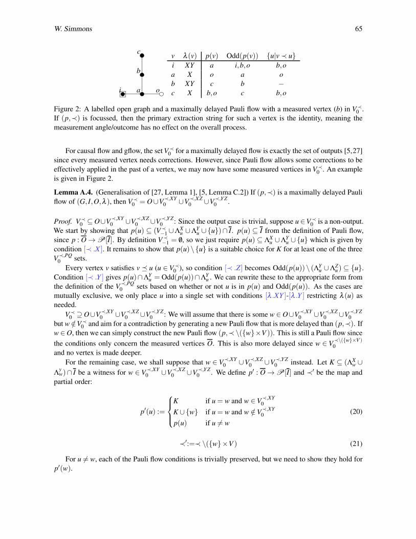
Figure 2: A labelled open graph and a maximally delayed Pauli flow with a measured vertex (b) in V≺0 .
If (p,≺) is focussed, then the primary extraction string for such a vertex is the identity, meaning the
measurement angle/outcome has no effect on the overall process.
For causal flow and gflow, the set V≺0 for a maximally delayed flow is exactly the set of outputs [5,27]
since every measured vertex needs corrections. However, since Pauli flow allows some corrections to be
effectively applied in the past of a vertex, we may now have some measured vertices in V≺0 . An example
is given in Figure 2.
Lemma A.4. (Generalisation of [27, Lemma 1], [5, Lemma C.2]) If (p,≺) is a maximally delayed Pauli
flow of (G, I,O,λ ), then V≺0 = O∪V
≺,XY0 ∪V
≺,XZ0 ∪V
≺,YZ0 .
Proof. V≺0 ⊆ O∪V
≺,XY0 ∪V
≺,XZ0 ∪V
≺,YZ0 : Since the output case is trivial, suppose u ∈V≺
0 is a non-output.
We start by showing that p(u) ⊆ (V≺−1 ∪ΛX
u ∪ΛYu ∪{u})∩ I. p(u) ⊆ I from the definition of Pauli flow,
since p : O → P[I]. By definition V≺−1 = /0, so we just require p(u) ⊆ ΛX
u ∪ΛYu ∪{u} which is given by
condition [≺ .X ]. It remains to show that p(u)\{u} is a suitable choice for K for at least one of the three
V≺,PQ
0 sets.
Every vertex v satisfies v � u (u ∈V≺0 ), so condition [≺ .Z] becomes Odd(p(u)) \ (ΛY
u ∪ΛZu ) ⊆ {u}.
Condition [≺ .Y ] gives p(u)∩ΛYu = Odd(p(u))∩ΛY
u . We can rewrite these to the appropriate form from
the definition of the V≺,PQ
0 sets based on whether or not u is in p(u) and Odd(p(u)). As the cases are
mutually exclusive, we only place u into a single set with conditions [λ .XY ]-[λ .Y ] restricting λ (u) as
needed.
V≺0 ⊇ O∪V
≺,XY0 ∪V
≺,XZ0 ∪V
≺,YZ0 : We will assume that there is some w ∈ O∪V
≺,XY0 ∪V
≺,XZ0 ∪V
≺,YZ0
but w /∈V≺0 and aim for a contradiction by generating a new Pauli flow that is more delayed than (p,≺). If
w ∈ O, then we can simply construct the new Pauli flow (p,≺ \({w}×V )). This is still a Pauli flow since
the conditions only concern the measured vertices O. This is also more delayed since w ∈ V≺\({w}×V )0
and no vertex is made deeper.
For the remaining case, we shall suppose that w ∈ V≺,XY0 ∪V
≺,XZ0 ∪V
≺,YZ0 instead. Let K ⊆ (ΛX
w ∪Λ
yw)∩ I be a witness for w ∈ V
≺,XY0 ∪V
≺,XZ0 ∪V
≺,YZ0 . We define p′ : O → P[I] and ≺′ be the map and
partial order:
p′(u) :=
K if u = w and w ∈V≺,XY0
K ∪{w} if u = w and w /∈V≺,XY0
p(u) if u 6= w
(20)
≺′:=≺ \({w}×V ) (21)
For u 6= w, each of the Pauli flow conditions is trivially preserved, but we need to show they hold for
p′(w).

66 Relating Measurement Patterns to Circuits via Pauli Flow
This satisfies condition [≺ .X ] from K ⊆ (ΛXw ∪ ΛY
w)∩ I. For each of the V≺,PQ0 options, we get
Odd(p′(w))\(
ΛYw ∪ΛZ
w
)
⊆{w}, so we can show [≺ .Z]. Similarly, we get p′(w)∩ΛYw =Odd(p′(w))∩ΛY
w
in each of the V≺,PQ
0 options, so condition [≺ .Y ] also follows.
The membership of w in p′(w) and Odd(p′(w)) is decided by which of the V≺,PQ0 it belongs to, which
also restricts λ (w) to the compatible planes according to conditions [λ .XY ]-[λ .Y ].
By assumption, w ∈ V≺k for some k > 0. By construction, the depth of every vertex under ≺′ is
no larger than its depth under ≺ and w ∈ V≺′0 . This means ∀k ≥ 0.
∣
∣V≺∪k
∣
∣ ≤∣
∣
∣V≺′∪k
∣
∣
∣and
∣
∣V≺0
∣
∣ <∣
∣
∣V≺′
0
∣
∣
∣, so
(p′,≺′) is a more delayed Pauli flow than (p,≺).
Lemma A.5. (Generalisation of [27, Lemma 3], [5, Lemma C.4]) If (p,≺) is a maximally delayed Pauli
flow of (G, I,O,λ ), then ∀k > 0.V≺k =V
≺,XYk ∪V
≺,XZk ∪V
≺,YZk .
Proof. For any given k, the proof of this follows the same strategy as Lemma A.4. When construct-
ing the more delayed flow given a counterexample w, we need to adapt the definition of ≺′ to ≺′:=(≺ \({w}×V ))∪ ({w}×V≺
∪k−1). Vertices in V≺∪k−1 are not covered by the constraints in the definitions
of V≺,PQk , so we add them all to the future of w to make sure we satisfy conditions [≺ .X ]-[≺ .Y ].
These characterisations of the sets V≺k give us an iterative method of identifying them since we can
simply search for possible witness sets K for each vertex.
Theorem A.6. (Restatement of Theorem 4.5) There exists an algorithm that decides whether a given
labelled open graph has a Pauli flow, and that outputs such a Pauli flow if it exists. Moreover, this output
is maximally delayed, and the algorithm completes deterministically in time that grows polynomially
with the number of vertices in the graph.
Proof. The function PauliFlow(V,Γ, I,O,λ ) in Algorithm 1 takes sets V and I,O ⊆ V of vertices, an
adjacency matrix Γ over V and a basis labelling function λ and returns “true” with a Pauli flow if one
exists and “false” otherwise.
To see this, we consider the auxilliary method PauliFlowAux(V,Γ, I,λ ,A,B,k) which aims to iden-
tify V≺k , given sets A = V≺
∪k−1 of possible correctors and B ⊆ V≺∪k (B ⊇ A) of solved vertices, and
then proceed recursively over the remainder of the graph for higher depths. For the case of k = 0,
O ⊆V≺0 has already been handled by the setup in PauliFlow(V,Γ, I,O,λ ) so it is sufficient to just find
V≺,XY
k ∪V≺,XZk ∪V
≺,YZk due to Lemma A.4. For k > 0, A=B so we are just finding V
≺,XYk ∪V
≺,XZk ∪V
≺,YZk
in accordance with Lemma A.5. In each recursive call, it examines each candidate vertex in turn and
looks for a witness set K for membership into either V≺,XYk , V
≺,XZk , or V
≺,YZk , from which we can identify
a valid correction set. The global variables p and d map vertices to their correction sets and depths from
the output (this defines the order ≺ over vertices with v ≺ w ⇔ d(v)> d(w)).
This algorithm is guaranteed to terminate because V is finite and B ⊆V strictly grows with each call
for k ≥ 1, so C will eventually be an empty set.
The resulting Pauli flow must be maximally delayed because we are constructing the largest set
possible at each value of k. If there were a more delayed Pauli flow (p′,≺′), there must be some minimal
k for which V≺′k \V≺
k is non-empty. However, if a vertex v belonged in this set then a suitable correction
set for v must exist. Algorithm 1 would find this when testing v and place it in V≺k .
For a given vertex u, finding the witness set K in each of the three possible search cases can be
achieved by solving the linear equation system MA,uXK = Sλ̃ in F2 defined by:

W. Simmons 67
PauliFlow(V,Γ, I,O,λ ) = begin
LX := /0; LY := /0; LZ := /0;
forall v ∈V do
if v ∈ O then d(v) := 0;
if λ (v) = X then LX := LX ∪{v};
if λ (v) = Y then LY := LY ∪{v};
if λ (v) = Z then LY := LZ ∪{v};
end
return PauliFlowAux(V,Γ, I,λ , /0,O,0);
end
PauliFlowAux(V,Γ, I,λ ,A,B,k) = begin
C := /0;
forall u ∈ BC do
if λ (u) ∈ {XY,X ,Y} then
KXY := Solution for K ⊆ (A∪LX ∪LY )∩ IC \{u} where
K ∩LY \ ({u}∪A) = Odd(K)∩LY \ ({u}∪A) and
Odd(K)∩ ((A∪LY ∪LZ)C ∪{u}) = {u};
end
if λ (u) ∈ {XZ,X ,Z} then
KXZ := {u}∪ (Solution for K ⊆ (A∪LX ∪LY )∩ IC \{u} where
K ∩LY \ ({u}∪A) = Odd(K ∪{u})∩LY \ ({u}∪A) and
Odd(K ∪{u})∩ ((A∪LY ∪LZ)C ∪{u}) = {u});
end
if λ (u) ∈ {Y Z,Y,Z} then
KYZ := {u}∪ (Solution for K ⊆ (A∪LX ∪LY)∩ IC \{u} where
K ∩LY \ ({u}∪A) = Odd(K ∪{u})∩LY \ ({u}∪A) and
Odd(K ∪{u})∩ ((A∪LY ∪LZ)C ∪{u}) = /0);
end
if a solution K0 is found for any of KXY ,KXZ,KYZ then
C :=C∪{u};
p(u) := K0;
d(u) := k;
end
end
if C = /0 and k > 0 then
if B =V then return (true, p,d);else return (false, /0, /0);
end
else
B′ := B∪C;
return PauliFlowAux(V,Γ, I,λ ,B′,B′,k+1);end
end
Algorithm 1: An algorithm for identifying whether a labelled open graph has a Pauli flow.

68 Relating Measurement Patterns to Circuits via Pauli Flow
MA,u :=
[
Γ∩KA,u×PA,u
(Γ+ Id)∩KA,u ×YA,u
]
(22)
Sλ̃ :=
[
{u}0
]
if λ̃ = XY
[
(NΓ(u)∩PA,u)∪{u}NΓ(u)∩YA,u
]
if λ̃ = XZ
[
NΓ(u)∩PA,u
NΓ(u)∩YA,u
]
if λ̃ = Y Z
(23)
where KA,u := (A∪ΛXu ∪ΛY
u )∩ IC is the set of possible elements of the witness set K, PA,u := (A∪ΛYu ∪
ΛZu )
C is the set of vertices in the past/present which should remain corrected afer measuring and correct-
ing u, YA,u := ΛYu \A is the set of vertices we have to consider for condition [≺ .Y ], λ̃ ∈ {XY,XZ,YZ}
denotes which of the three cases we are considering, and XK is the column vector with 1 in the position
of v if v ∈ K and a 0 otherwise.
Taking λ̃ = XY as an example, the top block of equations encodes Odd(K)∩PA,u = {u} and the
lower block encodes K ∩ΛYu \A = Odd(K)∩ΛY
u \A, so the solutions to these equations are exactly the
possible witness sets K. Such solutions can be identified by Gaussian elimination and back substitution
in O(|V |3) time.
This part of the algorithm is hit at most |V | times per call to PauliFlowAux, which may be called at
most |V | times, hence the overall complexity of this algorithm is O(|V |5).
The complexity of this algorithm is higher than the O(|V |4) for the equivalent method for identifying
gflow [5] 2. This is because we can no longer do a single gaussian elimination per depth round because
the matrix MA,u and the range of the witness set K are both dependent on the particular vertex u under
consideration.
B Focussed Sets and Pauli Flows
Even though the Pauli flow generated by Algorithm 1 is guaranteed to be maximally delayed, the correc-
tion sets may not be unique as the back substitution step may not have a single solution. In this section,
we will investigate some transformations on Pauli flows resulting from this freedom to show that we can
always reach a focussed Pauli flow.
Lemma B.1. Given a Pauli flow (p,≺) for a labelled open graph (G, I,O,λ ) with two vertices u,v ∈ O
such that u ≺ v, then (p′,≺) is a Pauli flow where p′(u) := p(u)∆p(v) and ∀w ∈ O\{u}.p′(w) := p(w).Moreover, if (p,≺) is maximally delayed, then so is (p′,≺).
Proof. The Pauli flow conditions hold trivially for any vertex in O\{u} since the correction sets have not
changed, so it is sufficient to show they are preserved for u. We should first observe that Odd(p′(u)) =Odd(p(u)∆p(v)) = Odd(p(u))∆Odd(p(v)).
[≺ .X ]: For any w ∈ p′(u) with w 6= u and λ (w) /∈ {X ,Y}, we must have either w ∈ p(u), w = v, or
w ∈ p(v)∧w 6= v. In any of these cases, we have u ≺ w from [≺ .X ] for (p,≺) and u ≺ v.
2It should be noted that Eslamy et al. provide an even more efficient algorithm for finding gflow in O(|V |3) time [17]. It
may be possible to generalise this to Pauli flow in search of a more efficient routine.

W. Simmons 69
[≺ .Z]: This follows similarly from u ≺ v and [≺ .Z] on Odd(p(u)) and Odd(p(v)).
[≺ .Y ]: For any w � u with λ (w) = Y , we also must have w � v since u ≺ v. Hence by [≺ .Y ],w ∈ p(u) ⇔ w ∈ Odd(p(u)) and the same for p(v). Therefore, we find that w ∈ p′(u) = p(u)∆p(v) ⇔w ∈ Odd(p(u))∆Odd(p(v)) = Odd(p′(u)) as required.
[λ .XY ]-[λ .Y Z]: u /∈ p(v) and u /∈ Odd(p(v)) by [≺ .X ] and [≺ .Z] since u ≺ v, so the requirements
are given by the corresponding conditions for (p,≺).
[λ .X ]: u /∈ Odd(p(v)) by [≺ .Z] and u ∈ Odd(p(u)) by [λ .X ], so u ∈ Odd(p′(u)).[λ .Z]: u /∈ p(v) by [≺ .X ] and u ∈ p(u) by [λ .Z], so u ∈ p′(u).[λ .Y ]: u ∈ p(v) ⇔ u ∈ Odd(p(v)) by [≺ .Y ] and u ∈ p(u) ⇔ u /∈ Odd(p(u)) by [λ .Y ], then it is
straightforward to show u ∈ p′(u)⇔ u /∈ Odd(p′(u)) by cases.
The maximally delayed property of a Pauli flow only concerns the partial order between the vertices,
so since (p,≺) and (p′,≺) both use ≺ the property is trivially preserved.
This gives us a mechanism to generate new Pauli flows by adding correction sets together. We now
show that this can help us to make progress towards satisfying the focussed property.
Lemma B.2. For any labelled open graph Γ, if sets p̂, q̂ ⊆ I are focussed over S ⊆ O, then so is p̂∆q̂.
Proof. [FX ]: For any vertex v ∈ (p̂∆q̂)∩ S, we have either v ∈ p̂ or v ∈ q̂. Since p̂ and q̂ are focussed
over S, the corresponding [FX ] condition gives λ (v) ∈ {XY,X ,Y}.
[FZ]: Similarly, for any vertex v ∈ Odd(p̂∆q̂)∩ S = (Odd(p̂)∆Odd(q̂))∩ S, λ (v) ∈ {XZ,YZ,Y,Z}follows from either v ∈ Odd(p̂) or v ∈ Odd(q̂) and [FZ].
[FY ]: For any v ∈ S with λ (v) =Y , we have v ∈ p̂ ⇔ v ∈ Odd(p̂) and v ∈ q̂ ⇔ v ∈ Odd(q̂) from [FY ]for p̂ and q̂. Hence v ∈ p̂∆q̂ ⇔ v ∈ Odd(p̂)∆Odd(q̂).
Lemma B.3. For any labelled open graph Γ, if sets p̂, q̂ ⊆ I are not focussed over {v} (v ∈ O), then p̂∆q̂
is focussed over {v}.
Proof. We consider each case for λ (v) and how the focussed conditions could fail for p̂ and q̂:
λ (v) ∈ {XY,X}: [FX ] and [FY ] are trivially satisfied, so we must have v ∈ Odd(p̂) and v ∈ Odd(q̂)to fail [FZ]. This means v /∈ Odd(p̂)∆Odd(q̂) = Odd(p̂∆q̂), satisfying [FZ] for p̂∆q̂.
λ (v) ∈ {XZ,Y Z,Z}: Similarly, [FZ] and [FY ] hold trivially, so we must have v ∈ p̂ and v ∈ q̂ to fail
[FX ]. We hence have v /∈ p̂∆q̂, satisfying [FZ] for p̂∆q̂.
λ (v) =Y : Now [FX ] and [FZ] are trivial and we have v ∈ p̂∆Odd(p̂) and v ∈ q̂∆Odd(q̂) to fail [FY ].This now satisfies [FY ] since v /∈ (p̂∆Odd(p̂))∆(q̂∆Odd(q̂)) = (p̂∆q̂)∆Odd(p̂∆q̂).
Combining these two lemmas, we can find combinations of correction sets that fix unfocussed ver-
tices whilst preserving those we have already focussed.
Lemma B.4. (Generalisation of [5, Lemma 3.13]) Let (G, I,O,λ ) be a labelled open graph with a Pauli
flow (p,≺) and some vertex v ∈ O. Then there exists p′ : O → P[I] such that:
1. ∀w ∈ O.v = w∨ p′(w) = p(w);
2. p′(v) is focussed over O\{v};
3. (p′,≺) is a Pauli flow for (G, I,O,λ ).
70 Relating Measurement Patterns to Circuits via Pauli Flow
Proof. Let J : Z|O| → O be some indexing of the vertices that respects the order ≺ (∀i, j < |O|.J(i) ≺J( j)⇒ i < j). We define a sequence of functions pk as:
p0(u) := p(u) (24)
pk+1(u) :=
pk(u)∆pk(J(k)) if
u = v,
J(k) 6= v,
pk(v) is not focussed over {J(k)}
pk(u) otherwise
(25)
1 is satisfied for all (pk,≺) by construction, and 3 is also satisfied for all by Lemma B.1. To work
towards 2, we proceed inductively with hypothesis Φ(k) := “pk(v) is focussed over {J(i)}i<k \{v}”. The
k = 0 case holds vacuously.
Suppose we have Φ(k). If J(k) = v, then pk+1(v) = pk(v) and Φ(k+1) is an immediate consequence
of Φ(k). If pk(v) is focussed over {J(k)}, then pk+1(v) = pk(v), so Φ(k+1) follows from this assumption
and Φ(k). If, on the other hand, pk(v) is not focussed over {J(k)}, we have pk+1(v) = pk(v)∆pk(J(k)).From conditions [λ .XY ]-[λ .Y ], pk(J(k)) is also not focussed over {J(k)}, so by Lemma B.3 we have
pk+1(v) is focussed over {J(k)}. For any of the remaining i < k (where J(i) 6= v), Φ(k) says that pk(v)is focussed over {J(i)}. Since J respects the order ≺, we also have J(i) � J(k), and hence conditions
[≺ .X ]-[≺ .Y ] imply that pk(J(k)) is focussed over {J(i)}. We combine these with Lemma B.2 to deduce
that pk+1(v) is also focussed over {J(i)}.
At the end of this chain, we have (p|O|,≺) where p|O| is focussed over O\{v}.
Lemma B.5. (Restatement of Lemma 4.6) If a labelled open graph has a Pauli flow, then it has a maxi-
mally delayed, focussed Pauli flow.
Proof. Let (p,≺) be such a maximally delayed Pauli flow according to Remark A.3. Applying Lemma
B.4 for each v ∈ O in turn, we reach some (p′,≺) where, for every v ∈ O, p′(v) is focussed over O\{v},
i.e. (p′,≺) is a focussed Pauli flow. Since the partial order ≺ remains the same, this is also still maximally
delayed.
For general measurement patterns, even focussed Pauli flows may not be unique. However, given
multiple focussed Pauli flows, the differences between their correction sets are given by the focussed sets
of the graph.
Lemma B.6. Let Γ = (G, I,O,λ ) be a labelled open graph with a focussed Pauli flow (p,≺) and a
focussed set p̂ ⊆ I. Let v ∈ O be a vertex such that ∀w ∈ p̂∪Odd(p̂).λ (w) ∈ {XY,XZ,YZ} ⇒ w 6=v∧ v � w. Then (p′,≺′) is a focussed Pauli flow, where:
p′(w) :=
{
p(w)∆ p̂ if w = v
p(w) if w 6= v(26)
and ≺′ is the transitive closure of ≺ ∪{(v,w)|w ∈ p̂∪Odd(p̂)∧λ (w) ∈ {XY,XZ,YZ}}.
Proof. Firstly, ≺′ is still a strict partial order. Transitivity is immediate from the definition as a transitive
closure. For antisymmetry (and similarly for strictness), suppose on the contrary that we have some
a ≺′ b and b ≺′ a (or directly a ≺′ a). This gives a transitive loop [a, . . . ,b, . . . ,a] where each step is

W. Simmons 71
either in ≺ or {(v,w)|w ∈ p̂∪Odd(p̂)∧ λ (w) ∈ {XY,XZ,YZ}}. Since ≺ is a strict partial order, we
cannot have such a loop where every step is in ≺, so at least one step must be some such (v,w). We can
freely eliminate inner loops around v, so we can assume wlog that v only appears once in the loop. This
means the rest of the loop is only from ≺, so w ≺ v by transitivity. However, we assumed that v � w
since w ∈ p̂∪Odd(p̂) and λ (w) ∈ {XY,XZ,YZ}, giving us the contradiction we need.
Conditions [≺ .X ]-[≺ .Y ] are preserved from the extension to ≺′ covering planar labels and the fo-
cussed property covering Pauli labels.
Conditions [λ .XY ]-[λ .Y Z] are preserved since v /∈ p̂∪Odd(p̂) gives v ∈ p′(v) ⇔ v ∈ p(v) and v ∈Odd(p′(v))⇔ v ∈ Odd(p(v)).
For conditions [λ .X ]-[λ .Y ], the correction amounts to saying that p′(v) is not focussed over {v}. If
this were not the case, then p′(v)∆ p̂ = p(v) would be focussed over {v} by Lemma B.2, contradicting
the corresponding Pauli flow condition for p(v).Finally, p′(v) is focussed over O\{v} using Lemma B.2, so (p′,≺′) is focussed.
Lemma B.7. Let Γ be a labelled open graph with two focussed Pauli flows (p,≺) and (p′,≺′). Then for
any vertex v ∈ O, p(v)∆p′(v) is a focussed set.
Proof. Each of p(v) and p′(v) are focussed over O\{v}, so their combination must also be by Lemma
B.2. For each case of λ (v), the corresponding condition from [λ .XY ]-[λ .Y ] is then enough to show that
p(v)∆p′(v) is also focussed over {v}.
An important consequence of this result is that in order to fully identify the space of all focussed
Pauli flows for a given labelled open graph, it is sufficient to find one using Algorithm 1 that we focus
with Lemma 4.6, and find all of the focussed sets. The following proofs show that the focussed sets
form a group, allowing us to only need some generating set, and giving an algorithm for finding such
generators.
Lemma B.8. The focussed sets of a labelled open graph form a group under ∆.
Proof. Closure is a direct consequence of Lemma B.2 with S = O. We then extend this to a group with
identity /0 and each focussed set is self-inverse.
Lemma B.9. Any labelled open graph Γ = (G, I,O,λ ) with a focussed Pauli flow has 2|O|−|I| distinct
focussed sets.
Proof. We can find the number of subsets of I that are focussed over some S ⊆ O inductively over the
size of S using the following induction hypothesis:
Φ(k) := ∀S ⊆ O.|S|= k ⇒∣
∣
{
p̂ ⊆ I∣
∣p̂ is focussed over S}∣
∣= 2|I|−|S| (27)
For k = 0, we only have to consider S = /0. Any subset of |I| satisfies the required properties, so there
are 2|I| many such sets, so Φ(0) holds.
Suppose Φ(k) holds for some k ≥ 0. Suppose S ⊆ O is of size k+1 and choose any vertex v ∈ S. Let
Sv := S\ v, so |Sv|= k. Φ(k) implies there are 2|I|−k subsets of I that are focussed over Sv. The subsets
focussed over S are those that are focussed over both Sv and {v}.
Let (p,≺) be some focussed Pauli flow for Γ, so p(v) is focussed over O\v, and hence for Sv. Lemma
B.2 implies the sets focussed over Sv are closed under symmetric difference with p(v). However, Lemma
B.3 implies p̂ is focussed over {p} if and only if p̂∆p(v) is not because p(v) corrects the measurement
at v. This means taking the symmetric difference with p(v) defines a bijection between the sets that are

72 Relating Measurement Patterns to Circuits via Pauli Flow
focussed for S and those that are focussed for Sv but not for {v}. Since these are disjoint and partition
the 2|I|−k that are focussed over Sv, we must have 2|I|−(k+1) that are focussed over S, giving Φ(k+1).
Focussed sets are those that are focussed over the entirety of O, so Φ(|O|) tells us that there are
2|I|−|O| = 2|O|−|I| focussed sets.
Lemma B.10. Given a labelled open graph Γ with focussed Pauli flow, there exists an algorithm that
identifies |O|−|I| independent generators for the group of focussed sets of Γ. Furthermore, this algorithm
completes in time polynomial in the number of vertices in Γ.
Proof. Similar to Theorem 4.5, we can encode the conditions for focussed sets into a linear equation
system MX = S in F2 which can be solved by Gaussian elimination and back substitution to obtain a
single focussed set.
M :=
[
Γ∩P×OC
(Γ+ Id)∩P×Y
]
(28)
S :=
[
0
0
]
(29)
P := (O∪{w ∈ O|λ (w) ∈ {XY,X ,Y}})∩ I (30)
O := O∪{w ∈ O|λ (w) ∈ {XZ,YZ,Y,Z}} (31)
Y := {w ∈ O|λ (w) = Y} (32)
In the above, we let Γ stand for the adjacency matrix of its graph. We define P to be the set of vertices
that could be included in a focussed set and O the set of vertices that could be in the odd neighbourhood.
Solutions satisfy [FX ] since X only ranges over P. The top block of the system encodes [FZ] since
multiplying by Γ in F2 gives the odd neighbourhood, and similarly the bottom block encodes [FY ].
We need to add additional conventions to make sure that the focussed sets we obtain are non-empty
and independent. Since this system is underconstrained (when there exist non-empty focussed sets),
there will always be some freedom of choice during the back substitution step. Since every focussed set
must be a solution, these free substitutions must generate the full set. Hence we can obtain independent,
non-empty focussed sets by taking a single free substitution for each focussed set, iterating through each
free substitution in turn.
Since both |P| and |OC|+ |Y| are at most |V |, the Gaussian elimination takes O(|V |3) time. Each
back substitution takes O(|V |2) time, which we must repeat |O|− |I| times giving O(|V |3) again.
It should be noted that similar conditions can be incorporated into Algorithm 1 to directly obtain
focussed Pauli flows by imposing further restrictions on the vertices that can be included in the correction
sets and adding extra equations to restrict the odd neighbourhood.
A final comment we will make about the focussed conditions is that it removes the need for any
ordering relation between Pauli vertices. When the measurement pattern uses only Pauli measurements,
all of them can be measured simultaneously, giving a single round of corrections on the outputs. When
there are additional planar measurements, we can do all Pauli measurements in a single layer before
considering any of the planar measurements.
Lemma B.11. If a labelled open graph has a Pauli flow, then there exists a Pauli flow (p,≺) which
satisfies ∀v ∈ O.λ (v) ∈ {X ,Y,Z}⇒ ∀u ∈V.v � u.

W. Simmons 73
Proof. Given a Pauli flow (p,≺), we can assume wlog that it is focussed from Lemma 4.6. Let ≺′:=≺\{(u,v) ∈V ×O|λ (v)∈{X ,Y,Z}}. By construction, this satisfies ∀v∈O.λ (v)∈ {X ,Y,Z}⇒∀u∈V.v �′
u. To show that (p,≺′) is a valid Pauli flow, we just need to show that [≺ .X ]-[≺ .Y ] are unaffected which
all follow from the focussed conditions.
C Proofs for Circuit Extraction
This section will explore how to identify extraction strings and their properties, building up to a proof
of Theorem 4.7 for circuit extraction. As dicussed in Section 4, the key principle is to extract planar
measurement angles as rotations over the outputs, to leave behind a stabilizer process. We start by
building up an explicit construction for extraction strings from a focussed Pauli flow.
Lemma C.1. Given a Pauli flow (p,≺) for a labelled open graph (G, I,O,λ ), for any vertex v ∈ O the
size of p(v)∩Odd(p(v)) is even.
Proof. Let G = (V,E) and define the subgraph G′ = (p(v),E ∩ (p(v)× p(v))). For any vertex w ∈ V ,
w ∈ p(v)∩Odd(p(v)) if and only if w has odd degree in G′. Since the sum of the vertex degrees must
equal 2 times the number of edges in G′, there must be an even number of vertices with odd degree.
Lemma C.2. (Restatement of Lemma 4.4) Let Γ = (G, I,O,λ ) be a labelled open graph with some
measurement angles α : O → [0,2π) and a focussed Pauli flow (p,≺). Then for any vertex v ∈ O, p(v)determines a P⊥v-extraction string.
Proof. Consider an arbitrary measured vertex v ∈ O.
Since each correction set p(v) is a subset of the non-input vertices, we can combine the graph state
stabilizers. We may reorder the Z and X terms with the possible introduction of a (−1).
EGNI = (−1)a
(
∏u∈p(v)
Xu
)(
∏u∈Odd(p(v))
Zu
)
EGNI (33)
where a = |E ∩ (p(v)× p(v))| is the number of edges in the subgraph of p(v), since for each edge here
we have to reorder the Z and X terms on exactly one of the two vertices.
There are an even number of vertices with both an X and a Z (see Lemma C.1), so we can apply
Y = iXZ on all such instances, again introducing a possible (−1) term.
EGNI = (−1)b
(
∏u∈p(v)\Odd(p(v))
Xu
)(
∏u∈Odd(p(v))\p(v)
Zu
)
(
∏u∈p(v)∩Odd(p(v))
Yu
)
EGNI
(34)
where b = a+ |p(v)∩Odd(p(v))|/2.
Since (p,≺) is a Pauli flow, every vertex in p(v) or Odd(p(v)) is either a Pauli measurement or
greater than v in ≺ (from conditions [≺ .X ] and [≺ .Z]). To fit the form from Equation 12, we consider
adding the corresponding projections. Since (p,≺) is focussed, each vertex (besides outputs and v) in
p(v) \Odd(p(v)) is projected into an X basis eigenvector, and similarly Odd(p(v)) \ p(v) into Z and

74 Relating Measurement Patterns to Circuits via Pauli Flow
p(v)∩Odd(p(v)) into Y . This means we can absorb these Pauli operators into the projections, again
with the possible introduction of a (−1).
∏u≻v
λ(u)/∈{X ,Y,Z}
〈+λ(u),0|u
∏u∈O\{v}
λ(u)∈{X ,Y,Z}
〈+λ(u),α(u)|u
EGNI
= (−1)c
∏u≻v
λ(u)/∈{X ,Y,Z}
〈+λ(u),0|u
∏u∈O\{v}
λ(u)∈{X ,Y,Z}
〈+λ(u),α(u)|u
(
∏u∈(p(v)\Odd(p(v)))∩(O∪{v})
Xu
)(
∏u∈(Odd(p(v))\p(v))∩(O∪{v})
Zu
)
(
∏u∈p(v)∩Odd(p(v))∩(O∪{v})
Yu
)
EGNI
(35)
where c = b+∣
∣(p(v)∪Odd(p(v)))∩{u ∈ O|λ (u) ∈ {X ,Y,Z}∧α(u) = π}∣
∣.
This is now a Pauli operator with P⊥v on v and remainder over only the outputs, making it a valid
primary extraction string.
Recall that the Product Rotation Lemma can use these extraction strings to remove the measurement
angles. We can summarise Equation 10 by
〈+λ(v),α(v)| ≈ 〈+λ(v),0|e(−1)Dv iα(v)
2P⊥v
(36)
Dv :=
{
1 if λ (v) =Y Z
0 otherwise(37)
where Dv dictates the direction of rotation about the Bloch sphere. This means the rotation we extract
over the outputs is e(−1)Dv i
α(v)2
P⊥v
.
After extracting all planar measurement angles, we are left with the following stabilizer process:
C =
∏u∈O
λ(u)/∈{X ,Y,Z}
〈+λ(u),0|u
∏u∈O
λ(u)∈{X ,Y,Z}
〈+λ(u),α(u)|u
EGNI (38)
We can characterise this by finding its isometry tableau. Recall from Section 3 that the isometry
tableau generalises variants of the stabilizer tableau representation from previous literature for both sta-
bilizer states [33], where the rows represent generators for the stabilizer group, and unitaries [1], where
the rows represent the actions of the unitary on Zu and Xu for each input u - that is, the operator P such
that PC Zu = C . It is enough for us to find such Zu and Xu actions for each input along with |O| − |I|generators for the free stabilizers over the outputs.
Since Z on an input will commute through the CZ gates, we can get the corresponding stablizer
row from the primary extraction string assuming P⊥u = Z for this input. This is guaranteed since the
correction set cannot contain any inputs, including itself.
W. Simmons 75
We can use the same trick to obtain the X rows from primary extraction strings. In this case, we find
an altered pattern (Γ′,α ′) such that C ≈ C ′Hu. The Hadamard maps X to a Z, meaning we can use the
extraction string with respect to (Γ′,α ′). One way to achieve this is by input extension.
Definition C.3 (Input Extension). Given an open graph (G, I,O), input extension about u ∈ I adds a
new vertex u′ that is only connected to u and replaces u in the input set. Formally, V ′ = V ∪ {u′},
E ′ = E ∪{u′ ∼ u}, I′ = (I ∪{u′})\{u}.
Lemma C.4. Let (Γ,α) describe a measurement pattern with some chosen input u ∈ I. Taking an
input extension about u gives an equivalent measurement pattern (Γ′,α ′) assuming λ ′ = λ ∪{u′ 7→ XY},
α ′ = α ∪{u′ 7→ 0}, and a Hamadard gate is applied to input u′ before the start of the pattern.
Proof. It is enough to verify the following equation:
H =√
2(〈+XY,0|⊗ I)CZ (I⊗|+X ,0〉) (39)
In order to actually use this, we need to show that Pauli flows are preserved by input extensions.
Lemma C.5. (Generalisation of [5, Lemma 3.8]) Let Γ and Γ′ be labelled open graphs related by an
input extension on vertex u ∈ I (generating u′ ∈ I′). If Γ has a Pauli flow, then so does Γ′.
Proof. Suppose Γ has a Pauli flow (p,≺). Let p′ = p∪{u′ 7→ {u}} and ≺′ be the transitive closure of
≺ ∪{(u′,w)|w ∈ NG(u)∪{u}}.
For any v ∈V \O, u′ /∈ p′(v) = p(v) and u′ /∈ OddG′(p′(v)) = OddG(p(v)) since its only neighbour u
is an input in Γ which could not appear in any correction sets from p. This allows us to inherit all of the
Pauli flow properties from (p,≺) for v as they have remained unchanged.
For u′, the definition of ≺′ guarantees conditions [≺ .X ]-[≺ .Y ] since u′ ≺′ w for every w ∈ NG(u)∪{u} = (OddG′(p′(u′))\{u′})∪ p′(u′). From the construction of p′(u′), we satisfy condition [λ .XY ], and
the remainder hold trivially.
The remaining stabilizer generators can be obtained from the focussed sets of the measurement pat-
tern.
Lemma C.6. Given a measurement pattern (Γ,α) where the labelled open graph Γ = (G, I,O,λ ) has a
focussed set p̂, then p̂ determines a stabilizer P̂ of the linear map:
∏w∈O
λ(w)/∈{X ,Y,Z}
〈+λ(w),0|w
∏w∈O
λ(w)∈{X ,Y,Z}
〈+λ(w),α(w)|w
EGNI (40)
Proof. This follows similarly to Lemma 4.4. After applying the measurement projections, the only Pauli
terms that are not absorbed into the projections are over the output qubits.
Lemma B.9 implies that we can get |O| − |I| generators for the group of focussed sets, and we
are looking for |O| − |I| generators for the free stabilizers. For this to work, we need the map from
Lemma C.6 to be a bijection (i.e. the generators for the focussed sets don’t degenerate when mapped
into stabilizers). We go one step further by showing that it also preserves the group action as a result of
Lemmas C.7 and C.8.
Lemma C.7. Let Γ be a labelled open graph. For any set of vertices S ⊆ I, denote the output substring
of the stabilizer as PS = (∏w∈O∩S Xw)(
∏w∈O∩Odd(S)Zw
)
. Then for any S,T ⊆ I we have PSPT ≈ PS∆T .
Proof. This follows from the anticommutativity of X and Z and Odd(S∆T ) = Odd(S)∆Odd(T ).

76 Relating Measurement Patterns to Circuits via Pauli Flow
PSPT =
(
∏w∈O∩S
Xw
)(
∏w∈O∩Odd(S)
Zw
)(
∏w∈O∩T
Xw
)(
∏w∈O∩Odd(T )
Zw
)
≈(
∏w∈O∩S
Xw
)(
∏w∈O∩T
Xw
)(
∏w∈O∩Odd(S)
Zw
)(
∏w∈O∩Odd(T )
Zw
)
=
(
∏w∈O∩(S∆T )
Xw
)(
∏w∈O∩Odd(S∆T )
Zw
)
= PS∆T
(41)
Lemma C.8. For any non-zero linear map C with stabilizers A and B, if A and B share the same Pauli
string then A = B.
Proof. If A and B share the same Pauli string, they can only differ by phase, so B= eiθ A. Since stabilizers
form a group, AB = A(eiθ A) = eiθ I is also a stabilizer, i.e. C = eiθ C . eiθ 6= 1 implies C is a zero map,
so we must have A = B.
Because the groups of focussed sets and free stabilizers have the same finite cardinality, injectivity
is enough to show that we have an isomorphism. We can prove this by showing that only the empty set
gets mapped to the identity.
Lemma C.9. Let (Γ,α) describe a measurement pattern with a focussed Pauli flow (p,≺). Then for any
vertices u,v ∈ O the primary extraction strings satisfy
P⊥uP⊥v = (−1)Fp
u→v+Fp
v→uP⊥vP⊥u (42)
where Fp
x→y := |{y}∩ (p(x)∪Odd(p(x)))| indicates whether y is used in the correction of x. Similarly,
given a focussed set p̂, its stabilizer satisfies
P⊥uP̂ = (−1)G p̂→uP̂P⊥u (43)
where G p̂→u = |{u}∩ (p̂∪Odd(p̂))| indicates whether u is used in the generation of the stabilizer.
Proof. Since P⊥u and P⊥v are tensor products of Pauli matrices, they must either commute or anticom-
mute. Consider the linear map C given by:
C :=
∏w∈O\{u,v}
λ(w)/∈{X ,Y,Z}u≺w∨v≺w
〈+λ(w),0|w
∏w∈O\{u,v}
λ(w)∈{X ,Y,Z}
〈+λ(w),α(w)|w
EGNI (44)
This may not be in the exact form needed to introduce extraction strings for u and v if they use each
other for corrections. Let Px→y be the Pauli induced on y when correcting x.

W. Simmons 77
Px→y :=
I if y /∈ p(x)∪Odd(p(x))
X if y ∈ p(x)\Odd(p(x))
Y if y ∈ p(x)∩Odd(p(x))
Z if y ∈ Odd(p(x))\ p(x)
(45)
We can still follow the construction in the proof of Lemma 4.4 to deduce that (−1)Apu→vP⊥u
u Pu→vv P⊥u
and (−1)Apv→u Pv→u
u P⊥vv P⊥v are stabilizers of C where
Apx→y :=
{
Fp
x→y if λ (y) ∈ {X ,Y,Z}∧α(y) = π
0 otherwise(46)
Comparing conditions [λ .XY ]-[λ .Y ] and the focussed conditions, we see that, for any vertex x ∈ O,
P⊥x is orthogonal to the measurement plane/Pauli of x and hence anticommutes with any Py→x 6= I.
Equationally, P⊥xPy→x = (−1)Fp
y→x Py→xP⊥x.
The stabilizer group of C is abelian, so we have
(−1)Apu→vP⊥u
u Pu→vv P⊥u(−1)A
pv→uPv→u
u P⊥vv P⊥v
=(−1)Apv→uPv→u
u P⊥vv P⊥v(−1)A
pu→v P⊥u
u Pu→vv P⊥u
=(−1)Fp
u→v+Fp
v→u(−1)Apu→vP⊥u
u Pu→vv P⊥v(−1)A
pv→u Pv→u
u P⊥vv P⊥u
(47)
i.e. P⊥uP⊥v = (−1)Fp
u→v+Fp
v→uP⊥vP⊥u.
The proof for focussed sets is virtually the same, though we only need care about anticommuting
Paulis on u.
Lemma C.10. Given a labelled open graph Γ = (G, I,O,λ ) with a focussed Pauli flow and any focussed
set p̂, then (p̂∪Odd(p̂))∩O = /0 ⇔ p̂ = /0.
Proof. p̂ = /0 ⇒ (p̂∪Odd(p̂))∩O = /0 is trivial. For the other direction, suppose for a contradiction that
we have a non-empty p̂ for which (p̂∪Odd(p̂))∩O= /0, so we have some v∈ p̂∩O and the corresponding
stabilizer is the identity. However, Lemma C.9 implies that the stabilizer must anticommute with the
primary extraction string P⊥v, contradicting the identity assumption.
Theorem C.11. Let (Γ,α) describe a measurement pattern with a focussed Pauli flow. Then the con-
struction from Lemma C.6 gives an isomorphism between the groups of focussed sets and the stabilizers
of the linear map for (Γ,α) after removing all planar measurement angles.
Proof. The group action is preserved due to Lemmas C.7 and C.8. By Lemma C.10, the map is injective
(if we had two distinct focussed sets with the same stabilizer, combining them with ∆ would give a non-
empty focussed set that maps to the identity stabilizer) and subsequently bijective by cardinality from
Lemma B.9.
This isomorphism guarantees that the focussed sets identified by Lemma B.10 actually give a gener-
ating set for the stabilizer group, giving a valid isometry tableau. All that remains is to put everything
together into a formal procedure.
78 Relating Measurement Patterns to Circuits via Pauli Flow
Theorem C.12. (Restatement of Theorem 4.7) Let (Γ,α) describe a measurement pattern where Γ has
a Pauli flow. Then there is an algorithm that identifies an equivalent circuit requiring no ancillae which
completes in time polynomial in the number of vertices in Γ.
Proof. Using Theorem 4.5 and Lemma 4.6, we can identify a maximally delayed, focussed Pauli flow
(p,≺). Let J : Z|O| → O be an indexing over the measured qubits such that J(i) ≺ J( j) ⇒ j < i, i.e. J
iterates from outputs to inputs respecting ≺. We will define a sequence of patterns (Γ,αk) and circuits
Ck such that JCkK · JΓ;αkK ≈ JΓ;αK (where J−K denotes the interpretation as a linear function). We start
with α0 = α and C0 is the empty (identity) circuit.
For any k ≥ 0, the update from αk to αk+1 is just setting the angle of J(k) to 0 if it is planar.
αk(J( j)) :=
{
0 if j < k∧λ (J(i)) ∈ {XY,XZ,YZ}α(J( j)) otherwise
(48)
Defining the update from Ck to Ck+1 requires us to find a Pauli string P over the outputs such that:
(
∏j<k∧λ(J( j))/∈{X ,Y,Z}
〈+λ(J( j)),0|J( j)
)
(
∏j≥k∨λ(J( j))∈{X ,Y,Z}
〈+λ(J( j)),α(J( j))|J( j)
)
EGNI
≈ eiα(J(k))
2P
(
∏j≤k∧λ(J( j))/∈{X ,Y,Z}
〈+λ(J( j)),0|J( j)
)
(
∏j>k∨λ(J( j))∈{X ,Y,Z}
〈+λ(J( j)),α(J( j))|J( j)
)
EGNI
(49)
When λ (J(k)) ∈ {X ,Y,Z} the projections on each side of Equation 49 are identical, meaning it
suffices to let P be the identity and set Ck+1 =Ck.
When λ (J(k)) ∈ {XY,XZ,YZ}, the projectors differ by a e(−1)
DJ(k) iα(J(k))
2P⊥J(k)J(k) according to Equa-
tion 10. Equation 49 then holds by using the Product Rotation Lemma with a primary extraction string
for J(k), which we can obtain by Lemma 4.4. We decompose this rotation into basic gates (for ex-
ample, by CX ladder constructions [6, 11]) and add them to the start of Ck so that JCk+1K = JCkK ·e(−1)
DJ(k) iα(J(k))
2P⊥J(k)
.
At the end of this sequence, we have the pattern (Γ,α|O|) where every measurement is in a Pauli
basis and the associated circuit C|O|. This means the corresponding isometry for this pattern is a stabilizer
process.
To characterise this process, it is sufficient to identify its isometry tableau. For each input, we can
find the Z row from the primary extraction string of the input vertex, and by taking an input extension
with Lemma C.5 we can similarly get the X row. Each of our |O|− |I| generators for the free stabilizers
is given by Lemma B.10.
We can efficiently synthesise the isometry tableau and qubit preparations into a circuit Cstab. The
final circuit is the combination of Cstab followed by C|O| which implements the same operator as (Γ,α).To examine the complexity, we suppose an explicit Pauli flow is not given up front. Theorem 4.5 says
that we can identify it in O(|V |5) time. We can extend the flow to consider all of the input extensions

W. Simmons 79
simultaneously using Lemma C.5 in O(|I|) time (ignoring the update to ≺ since it won’t affect the
outcome of the extraction procedure). The construction of Lemma 4.6 focusses this Pauli flow in O(|V |3)time (we apply at most O(|V |2) updates, each of which takes O(|V |) time to identify and apply). Adding
the extra focussed sets also takes O(|V |3) time by Lemma B.10. Synthesising this into a circuit using
the naive CX ladder construction takes O(|V | · |O|) time for the rotations from non-Pauli measurements,
and O(|O|3) to synthesise a stabilizer tableau using Aaronson and Gottesman’s method [1] (mapping
an isometry tableau into that form just requires identifying the additional generators to fill the Pauli
group, which can be done by Gaussian elimination in O(|O|3) time). The overall complexity is therefore
dominated by the O(|V |5) Pauli flow identification.
Example C.13. Suppose we start with the following measurement pattern and focussed Pauli flow.
i d
a
o2
c o1
b
v λ (v) p(v) Odd(p(v)) {u|v ≺ u}i XY b,o2 i,a a,b,c,o1,o2
a Y Z a,c,d,o2 d,o1,o2 c,o1,o2
b XY c,d,o1 b,d,o1,o2 c,o1,o2
c XY o1 c o1
d Y o2 d o2
Because we have two outputs and only one input, there is also an extra focussed set p̂ = {c,o2}. We
start by constructing the primary extraction strings for each vertex from Lemma 4.4. Let ad ∈ {0,1}be such that α(d) = adπ . Recall that we get one phase flip per edge between adjacent vertices in the
correction/focussed set (|E ∩ (p(v)× p(v))|), one phase flip for every two Y s that appear in the graph
state stabilizer (|p(v)∩Odd(p(v))|/2), and one for each term in the graph state stabilizer that is absorbed
from a Pauli measurement with angle π (|(p(v)∪Odd(p(v)))∩{w|λ (w) ∈ {X ,Y,Z}∧α(w) = π}|).
S S∩O Odd(S)∩O Edges Y s Paulis PS
p(i) o2 0 0 I1X2
p(a) o2 o1,o2 4 2 d (−1)ad+1Z1Y2
p(b) o1 o1,o2 2 2 d (−1)ad+1Y1Z2
p(c) o1 0 0 X1I2
p(d) o2 0 0 I1X2
p̂ o2 o1 0 0 Z1X2
We start by extracting the planar angles as rotations in ≻-order. We must start with c, extracing it as
eiα(c)
2X1I2 over the outputs.
Having extracted this, the projection on c becomes the positive X basis vector so it can absorb the
corresponding Paulis on the graph state stabilizer from p(a) and p(b). Either a or b can be extracted
next, giving e(−1)ad
α(a)2
Z1Y2 and e(−1)ad+1 α(b)
2Y1Z2 respectively. Note that the phase of the rotation from a
got an extra −1 since Da = 1 (λ (a) = Y Z).
The final rotation to be extracted is eiα(i)
2I1X2 from i. We don’t extract any rotation from d since the
measurement is already in a Pauli basis, and hence we can treat it as part of the leftover stabilizer process.
We can get the isometry tableau for this from the primary extraction strings. Having both the input
and its only neighbour labelled with XY means we don’t necessarily have to perform input extensions
to obtain the rows of the tableau during extraction, since they will function identically to i and b here
because Γ can already be viewed as an input extension of Γ \{i} with input b. This process maps Z on
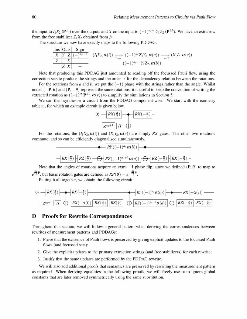
80 Relating Measurement Patterns to Circuits via Pauli Flow
the input to I1X2 (P⊥i) over the outputs and X on the input to (−1)ad+1Y1Z2 (P⊥b). We have an extra row
from the free stabilizer Z1X2 obtained from p̂.
The structure we now have exactly maps to the following PDDAG:
Ins Outs Sign
X Y Z (−)ad+1
Z X +
Z X +
(I1X2,α(i)) ((−1)ad Z1Y2,α(a)) (X1I2,α(c))
((−1)ad+1Y1Z2,α(b))
Note that producing this PDDAG just amounted to reading off the focussed Pauli flow, using the
correction sets to produce the strings and the order ≺ for the dependency relation between the rotations.
For the rotations from a and b, we put the (−1) phase with the strings rather than the angle. Whilst
nodes (−P,θ) and (P,−θ) represent the same rotations, it is useful to keep the convention of writing the
extracted rotation as ((−1)Dv P⊥v,α(v)) to simplify the simulations in Section 5.
We can then synthesise a circuit from the PDDAG component-wise. We start with the isometry
tableau, for which an example circuit is given below.
RX(π2) RX(−π
2)
Zad+1 H
|0〉
For the rotations, the (I1X2,α(i)) and (X1I2,α(c)) are simply RX gates. The other two rotations
commute, and so can be efficiently diagonalised simultaneously.
RY ((−1)ad α(b))
RZ((−1)ad+1α(a))RZ(π2) RZ(−π
2)RX(π
2) RX(−π
2)
Note that the angles of rotations acquire an extra −1 phase flip, since we defined (P,θ) to map to
eiθ2
P, but basic rotation gates are defined as RP(θ) = e−i
θ2
P.
Putting it all together, we obtain the following circuit:
RX(π2) RX(−π
2)
Zad+1 H
|0〉 RY ((−1)ad α(b))
RZ((−1)ad+1α(a))RZ(π2) RZ(−π
2)RX(π
2) RX(−π
2)RX(−α(i))
RX(−α(c))
D Proofs for Rewrite Correspondences
Throughout this section, we will follow a general pattern when deriving the correspondences between
rewrites of measurement patterns and PDDAGs:
1. Prove that the existence of Pauli flows is preserved by giving explicit updates to the focussed Pauli
flows (and focussed sets);
2. Give the explicit updates to the primary extraction strings (and free stabilizers) for each rewrite;
3. Justify that the same updates are performed by the PDDAG rewrite.
We will also add additional proofs that semantics are preserved by rewriting the measurement pattern
as required. When deriving equalities in the following proofs, we will freely use ≈ to ignore global
constants that are later removed symmetrically using the same substitution.

W. Simmons 81
D.1 Relabelling Pauli Measurements
Lemma D.1. Let (Γ,α) describe a measurement pattern and u∈O be a vertex with λ (u)∈ {XY,XZ,YZ}and α(u) ∈ {0, π
2,π, 3π
2}. Then there exists an equivalent pattern (Γ′,α ′) from relabelling u as a Pauli
measurement, where the new labels and angles are given by
(λ ′(u),α ′(u)) =
(X ,α(u)) if λ (u) = XY ∧α(u) ∈ {0,π}(Y,α(u)− π
2) if λ (u) = XY ∧α(u) ∈ {π
2, 3π
2}
(Z,α(u)) if λ (u) = XZ∧α(u) ∈ {0,π}(X ,α(u)− π
2) if λ (u) = XZ∧α(u) ∈ {π
2, 3π
2}
(Z,α(u)) if λ (u) = Y Z∧α(u) ∈ {0,π}(Y,α(u)− π
2) if λ (u) = Y Z∧α(u) ∈ {π
2, 3π
2}
(50)
and (λ ′(v),α ′(v)) = (λ (v),α(v)) for any v ∈ O\{u}.
Proof. The following equations describe how the Pauli measurements are embedded into the planes:
〈+X ,α | ≈ 〈+XY,α | ≈ 〈+XZ,α+
π2|
〈+Y,α | ≈ 〈+XY,α+
π2| ≈ 〈+
YZ,α+π2|
〈+Z,α | ≈ 〈+XZ,α | ≈ 〈+YZ,α |
(51)
The equivalent Pauli measurement label and angle are determined uniquely by these embeddings.
Lemma D.2. Let (Γ,α) and (Γ′,α ′) describe measurement patterns related by relabelling some planar
u ∈O as a Pauli according to Lemma D.1. If Γ has a focussed Pauli flow (p,≺), then (p′,≺) is a focussed
Pauli flow for Γ′ where for any v ∈ O
p′(v) :=
{
p(v)∆p(u) if v 6= u∧u ∈ p(v)∪Odd(p(v))∧α(u) ∈ {π2, 3π
2}
p(v) otherwise(52)
Furthermore, focussed sets p̂ can be updated as
p̂′ :=
{
p̂∆p(u) if u ∈ p̂∪Odd(p̂)∧α(u) ∈ {π2, 3π
2}
p̂ otherwise(53)
Proof. Suppose that (p,≺) is a focussed Pauli flow for Γ. Since λ (u) ∈ {XY,XZ,YZ}, any v ∈ O\{u}such that u ∈ p(v)∪Odd(p(v)) must satisfy v ≺ u by conditions [≺ .X ] and [≺ .Z]. (p′,≺) is then also a
Pauli flow for Γ using Lemma B.1. Any Pauli flow for Γ is also a Pauli flow for Γ′, since [≺ .X ]-[≺ .Y ]are strictly weakened and [λ .X ]-[λ .Y ] for Γ′ follow from [λ .XY ]-[λ .Y Z] for Γ.
To show that (p′,≺) is focussed for Γ′, consider and vertex v ∈ O. As λ and λ ′ only differ on u, when
p′(v)= p(v) it remains focussed over O\{u,v} in Γ′. This is enough when v= u. If u /∈ p(v)∪Odd(p(v)),then it is trivially focussed over {u} in Γ′. Finally, in each of the cases of Equation 50 where α(u) ∈{0,π}, the compatible corrections in the focussed conditions do not change, so it remains focussed over
{u} in Γ′.

82 Relating Measurement Patterns to Circuits via Pauli Flow
Suppose instead that v 6= u, u ∈ p(v)∪Odd(p(v)), and α(u) ∈ {π2, 3π
2}, so p′(v) = p(v)∆p(u). Both
p(v) and p(u) remain focussed over O\{u,v} in Γ′, and Lemma B.2 gives the same for p′(v). For each
case of λ (u)∈ {XY,XZ,YZ}, what was a compatible correction for λ (u) is now incompatible with λ ′(u),so p(v) is not focussed over {u} in Γ′. Additionally, conditions [λ .X ] and [λ .Y ] mean that p(u) is also
not focussed over {u}. However, we can then use Lemma B.3 to conclude that their combination (p′(v))is focussed.
The proof of updating a focussed set p̂ to p̂′ follows similarly.
Lemma D.3. Let (Γ,α) and (Γ′,α ′) be the measurement patterns and respective focussed Pauli flows
(p,≺) and (p′,≺) from Lemma D.2 formed by changing the label of some u ∈ O from a planar measure-
ment to a Pauli measurement. Then the new primary extraction string for each vertex v ∈ O\{u} is given
by
P′⊥v= P′⊥v
v P⊥vv P⊥v
(
cosα(u)I − isin(−1)Du+Apu→vα(u)Pu→v
v P⊥u)F
pv→u
(54)
and P′⊥u = P⊥u. Furthermore, a stabilizer from a focussed set p̂ is updated to
P̂′ = P̂(
cosα(u)I − isin(−1)Du α(u)P⊥u)G p̂→u
(55)
Proof. The case for u is simple because p′(u) = p(u) and the linear map C in the definition of extraction
strings is unchanged. For the remainder, we consider some v ∈ O\{u}.
Firstly, we show that P′⊥vP⊥v ≈ I if α(u) ∈ {0,π} or (Pu→v)Fp
v→u if α(u) ∈ {π2, 3π
2} to deduce that
P′⊥vonly acts on the outputs. If either u /∈ p(v)∪Odd(p(v)) (i.e. F
pv→u = 0) or α(u) ∈ {0,π}, then
p′(v) = p(v) and hence P′⊥v = P⊥v. Otherwise, we have p′(v) = p(v)∆p(u). By following a similar
logic to the proof of Lemma C.7 considering {v} instead of O, we end up with P′⊥v ≈ P⊥vPu→v.
Now we show that P′⊥vis a primary extraction string in (Γ′,α ′). Let C ′ be the linear map from
Definition 4.2 for (Γ′,α ′) and let C be the corresponding for (Γ,α) (plus an extra projection on u if
u � v).
C′ :=
∏w≻v
λ ′(w)/∈{X ,Y,Z}
〈+λ ′(w),0|w
∏w∈O\{v}
λ ′(w)∈{X ,Y,Z}
〈+λ ′(w),α ′(w)|w
EGNI
≈ 〈+λ(u),α(u)|u
∏w≻vw6=u
λ(w)/∈{X ,Y,Z}
〈+λ(w),0|w
∏w∈O\{v}
λ(w)∈{X ,Y,Z}
〈+λ(w),α(w)|w
EGNI
≈
∏w≻v∨w=u
λ(w)/∈{X ,Y,Z}
〈+λ(w),0|w
∏w∈O\{v}
λ(w)∈{X ,Y,Z}
〈+λ(w),α(w)|w
e(−1)Du i
α(u)2
P⊥uu EGNI
= e(−1)Du+A
pu→v i
α(u)2
Pu→vv P⊥u
C (56)
= e(−1)Du+A
pu→v i
α(u)2
Pu→vv P⊥u
P⊥vv P⊥v
C

W. Simmons 83
= P⊥vv e
(−1)Du+Apu→v+F
pu→v i
α(u)2
Pu→vv P⊥u
P⊥vC
= P⊥vv P⊥ve
(−1)Du+Apu→v+F
pv→u i
α(u)2
Pu→vv P⊥u
C
= P⊥vv P⊥ve−(−1)Du+A
pu→v F
pv→uiα(u)Pu→v
v P⊥u
e(−1)Du+A
pu→v i
α(u)2
Pu→vv P⊥u
C
≈ P⊥vv P⊥ve−(−1)Du+A
pu→v F
pv→uiα(u)Pu→v
v P⊥u
C′
= P⊥vv P⊥v
(
cos α(u)I − isin(−1)Du+Apu→vα(u)Pu→v
v P⊥u)F
pv→u
C′
= P′⊥vv P′⊥v
C′
In the above derivation, moving P⊥vv P⊥v through the rotation requires Lemma C.9 and P⊥vPu→v =
(−1)Fp
u→vPu→vP⊥v.
Finally, by doing a case distinction on Fp
v→u and Lemma C.7, the extraction string from (p′,≺)matches P′⊥v
up to phase, with Lemma C.8 making them equal.
The proof for focussed sets and stabilizers follows similarly.
Theorem D.4. (Restatement of Theorem 5.1) Let (Γ,α) describe a measurement pattern with some
vertex u ∈ O such that λ (u) ∈ {XY,XZ,YZ} and α(u) ∈ {0, π2,π, 3π
2}. Relabelling u to the equivalent
Pauli label corresponds to pushing the rotation from u to the start of the PDDAG and absorbing it into
the initial stabilizer process.
Proof. The corresponding PDDAG initially has a rotation node ((−1)Du P⊥u,α(u)) (representing the
operator e(−1)Du i
α(u)2
P⊥u
) since u originally has a planar label. Moving this to the front of the circuit
updates the Pauli strings of other vertices according to the Reorder Rules, so we need to check that the
same update is made to planar vertices and the isometry tableau is updated appropriately.
For any planar vertex v � u, v /∈ p(u)∪Odd(p(u)) and hence Pu→v = I and Apu→v = 0. If u /∈ p(v)∪
Odd(p(v)) then P⊥v and P⊥u commute, so no update is needed which matches the formula for P′⊥vwith
Fp
v→u = 0. Otherwise, they anticommute. If α(u) = 0, the rotation is an identity so P⊥v is unchanged. If
α(u) = π , the rotation is a Pauli operator and hence flips the phase of v’s rotation, matching the cosα(u)update. For α(u) ∈ {π
2, 3π
2}, the extraction string is updated by multiplication with the correct phase.
For the tableau, we need to handle rows from both the inputs and free stabilizers. For an input
i gained by input extension with λ (i) = XY , the same reductions can be made as for planar vertices
and the updates for free stabilizers are essentially identical. In each case of α(u), these updates match
the effect on the isometry tableau since the Reorder Rules show the same effect for Paulis and generic
rotations.
Example D.5. Let’s start with the same measurement pattern from Example C.13. Suppose α(c) = π2
,
so we can obtain a semantically equivalent pattern by relabelling (λ ′(c),α ′(c)) := (Y,0). This would
make p(a), p(b) and p̂ no longer focussed. Refocussing gives:
v λ ′(v) p′(v) Odd(p′(v)) {u|v ≺′ u}i XY b,o2 i,a a,b,o1,o2
a Y Z a,c,d,o1,o2 c,d,o1,o2 o1,o2
b XY c,d b,c,d,o1,o2 o1,o2
c Y o1 c o1
d Y o2 d o2

84 Relating Measurement Patterns to Circuits via Pauli Flow
and p̂′ = {c,o1,o2}. The restriction of ≺ to ≺′ is not necessary, but will help to see the resemblance to
the PDDAG later.
Now let’s look at applying the corresponding rewrite on the PDDAG from C.13. That is, we use
the Reorder Rules to move (X1I2,π2) (i.e. e
iπ4
X1I2) into the tableau. X1I2 anticommutes with the rotations
from a and b, the tableau row from b, and the free stabilizer from p̂. Each of these strings will then be
updated by multiplication by X1I2. These are exactly the correction/focussed sets that were updated in
the measurement pattern by combining with p(c). The result of this rewrite on the PDDAG is:
Ins Outs Sign
X Z Z (−)ad
Z X +
Y X +
(I1X2,α(i)) ((−1)ad+1Y1Y2,α(a))
((−1)ad Z1Z2,α(b))
One can check that this is identical to the PDDAG extracted using (p′,≺).
D.2 Z Measurement Elimination
Lemma D.6. Let (Γ,α) describe a measurement pattern with some vertex u ∈ O such that λ (u) ∈{XZ,Y Z,Z} and α(u) = aπ (a ∈ {0,1}). Then eliminating vertex u gives an equivalent measurement
pattern (Γ′,α ′) where Γ′ = (G\{u}, I,O,λ ), for all w ∈ O\{u}
α ′(w) :=
α(w)+aπ if w ∈ NG(u)∧λ (w) ∈ {XY,X ,Y}(−1)aα(w) if w ∈ NG(u)∧λ (w) ∈ {XZ,YZ}α(w) otherwise
(57)
and each output neighbouring u is followed by a Za gate.
Proof. This is just an extension of the planar case given in the proof of [5, Lemma 4.7] to cover Pauli
labels by considering the embeddings from Equation 51. The idea is that the Z-basis projections 〈0|and 〈1| reduce each of the CZ gates on that qubit to either an identity or a Z gate (modelled as a Z
conditioned on the measurement angle), in the same way that they reduce when applied to a |0〉 or |1〉.This Z commutes with other CZ gates to the neighbouring outputs or to change the effective measurement
on the neighbour. The qubit u can then be removed since the only operations on it are the preparation
and measurement.
Lemma D.7. (Generalisation of [5, Lemma 3.4]) Let (Γ,α) and (Γ′,α ′) be measurement patterns related
by elimination of a vertex u as in Lemma D.6. If (p,≺) is a Pauli flow for Γ, then (p′,≺) is a Pauli flow
for Γ′ where for any v ∈ O\{u}
p′(v) :=
{
p(v)∆p(u) if u ∈ p(v)
p(v) if u /∈ p(v)(58)
If (p,≺) is focussed, then so is (p′,≺). Furthermore, if p̂ is a focussed set for Γ, then it is also a
focussed set for Γ′.
Proof. We first need to show that p′ is a function from O\{u} to P[I \{u}]. This follows since λ (u) ∈{XZ,Y Z,Z} implies u ∈ p(u) (by conditions [λ .XZ], [λ .Y Z], and [λ .Z]), so both cases of the definition
of p′(v) give u /∈ p′(v).

W. Simmons 85
Because λ (u) ∈ {XZ,Y Z,Z}, if u ∈ p(v) then v ≺ u from [≺ .X ]. This means (p′,≺) is a valid Pauli
flow for (G, I,O,λ ) by repeated applications of Lemma B.1. In particular, this means it satisfies all of
the Pauli flow conditions for any v ∈ O\{u}. These aren’t invalidated when restricting to G\{u} since
OddG\{u}(A) = OddG(A)\{u} for any A ⊆V \{u} and ∀v ∈ O\{u}.p′(v)⊆V \{u}.
If (p,≺) is a focussed Pauli flow, then u /∈ p(v) for any v 6= u since λ (u) ∈ {XZ,Y Z,Z}. This means
p′(v) = p(v) for every v, so the focussed property is trivially preserved. Similarly, the same holds for
focussed sets.
Lemma D.8. Let (Γ,α) and (Γ′,α ′) be the measurement patterns and respective Pauli flows (p,≺) and
(p′,≺) from Lemma D.7 formed by the elimination of a vertex u. Then the new primary extraction string
for each vertex v ∈ O\{u} is given by
P′⊥v= (−1)a|p(v)∩NG(u)∩(O∪{v})|
∏n∈(NG(u)∪{u})∩O
n≻vn=u⇒λ(n)∈{XZ,Y Z}
n6=u⇒λ(n)=XY
(−1)Fp
v→n
a
P⊥v (59)
where α(u) = aπ . Furthermore, the stabilizer from a focussed set p̂ is updated similarly.
Proof. The focussed property implies u /∈ p(v) (resp. u /∈ p̂), so p′(v) = p(v) (resp. p̂ is still a focussed
set). Then p′(v)∪OddG\u(p′(v)) = (p(v)∪OddG(p(v)))\{u} (resp. p̂∪OddG\u(p̂) = (p̂∪OddG(p̂))\{u}). This is enough to show that the strings are preserved up to phase.
We find a primary extraction string for v in (Γ′,α ′) by considering the linear map C ′ from Definition
4.2, using the respective linear map C for (Γ,α).
C′ =
∏w≻vw6=u
λ(w)/∈{X ,Y,Z}
〈+λ(w),0|w
∏w∈O\{u}
λ(w)∈{X ,Y,Z}
〈+λ(w),α ′(w)|w
EG\uNI\{u} (60)
We can reintroduce qubit u with measurement angle 0. We can then map the angles for the Pauli
projections from α ′ to α using orthogonal Paulis, letting zu := 1 if λ (u) = Z and 0 if λ (u) ∈ {XZ,Y Z}.
C′ ≈
√2
∏w≻vw6=u
λ(w)/∈{X ,Y,Z}
〈+λ(w),0|w
∏w∈O\{u}
λ(w)∈{X ,Y,Z}
〈+λ(w),α ′(w)|w
〈+λ(u),0|u EGNI
≈√
2
∏w≻v∨w=u
λ(w)/∈{X ,Y,Z}
〈+λ(w),0|w
∏w∈O
λ(w)∈{X ,Y,Z}
〈+λ(w),α(w)|w
(P⊥uu )zua
∏n∈NG(u)
λ(n)∈{X ,Y}
P⊥nn
a
EGNI
(61)

86 Relating Measurement Patterns to Circuits via Pauli Flow
We can then apply the stabilizer of the graph state centred around u to move these Paulis to other
qubits, some of which can be absorbed into projections again.
C′ ≈
√2
∏w≻v
λ(w)/∈{X ,Y,Z}
〈+λ(w),0|w
∏w∈O
λ(w)∈{X ,Y,Z}
〈+λ(w),α(w)|w
(P⊥uu )(1−zu)a
(
∏n∈NG(u)∩(O∪{v})
Zn
)a
∏n∈NG(u)∩O
n≻vλ(n)=XY
P⊥nn
a
∏n∈NG(u)∩O
n�vλ(n)/∈{X ,Y,Z}
Zn
a
EGNI
(62)
Each of the Paulis trapped under projections can be replaced by the primary extraction strings of
those qubits. We leave the extraction strings without any order since reordering only introduces phases
at this point which will be later removed.
C′ ≈
√2
∏w=uw≻v
Pu→vv P⊥u ∏
w=uw�v
P⊥uu
(1−zu)a(
∏n∈NG(u)∩(O∪{v})
Zn
)a
∏n∈NG(u)∩O
n≻vλ(n)=XY
Pn→vv P⊥n
a
∏n∈NG(u)∩O
n�vλ(n)/∈{X ,Y,Z}
Zn
a
C
(63)
We can now introduce P⊥vv P⊥v. Commuting this to the front induces phase changes according to
Lemma C.9 and P⊥vPu→v = (−1)Fp
u→v Pu→vP⊥v. We then undo the previous steps to get back to C ′.
C′ ≈
√2
∏w=uw≻v
Pu→vv P⊥u ∏
w=uw�v
P⊥uu
(1−zu)a(
∏n∈NG(u)∩(O∪{v})
Zn
)a
∏n∈NG(u)∩O
n≻vλ(n)=XY
Pn→vv P⊥n
a
∏n∈NG(u)∩O
n�vλ(n)/∈{X ,Y,Z}
Zn
a
P⊥vv P⊥v
C
=√
2P⊥vv
∏w=uw≻v
(−1)Fp
u→v Pu→vv P⊥u ∏
w=uw�v
P⊥uu
(1−zu)a
(64)
(−1)a|p(v)∩NG(u)∩{v}|(
∏n∈NG(u)∩(O∪{v})
Zn
)a

W. Simmons 87
∏n∈NG(u)∩O
n≻vλ(n)=XY
(−1)Fp
n→v Pn→vv P⊥n
a
∏n∈NG(u)∩O
n�vλ(n)/∈{X ,Y,Z}
Zn
a
P⊥vC
=√
2P⊥vv P⊥v
∏w=uw≻v
(−1)Fp
v→u Pu→vv P⊥u ∏
w=uw�v
P⊥uu
(1−zu)a
(−1)a|p(v)∩NG(u)∩(O∪{v})|(
∏n∈NG(u)∩(O∪{v})
Zn
)a
∏n∈NG(u)∩O
n≻vλ(n)=XY
(−1)Fp
v→n Pn→vv P⊥n
a
∏n∈NG(u)∩O
n�vλ(n)/∈{X ,Y,Z}
Zn
a
C
≈P⊥vv P⊥v(−1)a|p(v)∩NG(u)∩(O∪{v})|
∏n∈(NG(u)∪{u})∩O
n≻vn=u⇒λ(n)∈{XZ,Y Z}
n6=u⇒λ(n)=XY
(−1)Fp
v→n
a
C′
The calculations for focussed sets follow similarly. We can finish by using Lemma C.8 to conclude
that these primary extraction strings (resp. stabilizers) are the ones generated by the new Pauli flow (resp.
focussed sets).
Theorem D.9. (Restatement of Theorem 5.2) Let (Γ,α) describe a measurement pattern with some
vertex u ∈ O such that λ (u) ∈ {XZ,YZ,Z} and α(u) ∈ {0,π}. Eliminating u from the graph corresponds
to the following sequence of actions on the PDDAG:
1. If u has a planar (XZ or Y Z) label, then its rotation is pulled from the rotation DAG into the
stabilizer block;
2. For each neighbour n of u that is an output, a Zn rotation of α(u) is pulled from the stabilizer block
through the entire rotation DAG to the end of the circuit;
3. For each neighbour n of u with λ (n) = XY , a P⊥n rotation of α(u) is pulled from the stabilizer
block and merged with the existing rotation for n.
Proof. Each action is moving Pauli operators through rotations. The Reorder Rules simplify to inducing
phase flips. In the PDDAG, we can flip either the operator or angle of the rotation. The α(u) = 0 case is
trivial, so we suppose that α(u) = π (a = 1).
For both the rotations and tableau rows, we need only consider extraction strings of planar vertices.
Each of the rotations moved through the PDDAG to/from location w (either w = u or w ∈ NG(u)) would
induce a phase shift in the rotation or tableau row for v if the corresponding Pauli string P⊥w anticom-
mutes with P⊥v and originated beyond v (either w is an output or v � w), i.e. w ∈ p(v)∩O or Fp
v→w = 1.

88 Relating Measurement Patterns to Circuits via Pauli Flow
Equation 59 also negates the angle on v if v ∈ NG(u) and λ (v) ∈ {XZ,Y Z} (i.e. v ∈ p(v)), as covered in
Lemma D.6.
Example D.10. We will use the same example measurement pattern as Example C.13. a is the only
vertex with a label ready for vertex elimination, so to see something actually interesting we suppose
α(a) = π . Eliminating a gives the following residual pattern.
i d o2
c o1
b
v λ ′(v) α ′(v) p′(v) Odd(p′(v)) {u|v ≺ u}i XY α(i) b,o2 i b,c,o1,o2
b XY α(b)+π c,d,o1 b,d,o1,o2 c,o1,o2
c XY α(c)+π o1 c o1
d Y α(d)+π o2 d o2
The focussed set p̂ = {c,o2} remains valid. Following the rewrite sequence in the PDDAG, step
1 sees the rotation from a pulled into the tableau. The Z1Y2 term anticommutes with the rotation and
tableau row from i, as well as the free stabilizer from p̂.
Ins Outs Sign
X Y Z (−)ad+1
Z X −Z X −
(−I1X2,α(i)) ((−1)ad+1Y1Z2,α(b)) (X1I2,α(c))
For step 2, none of the neighbours of a are outputs, so there is no change. For step 3, only b and c are
labelled XY , so we move Y1Z2 and X1I2 from the tableau and merge into their corresponding rotations.
Ins Outs Sign
X Y Z (−)ad
Z X +
Z X +
(I1X2,α′(i)) ((−1)adY1Z2,α
′(b)) (X1I2,α′(c))
This same PDDAG is obtained by extracting from the reduced measurement pattern above. Since
extraction will give everything in terms of α ′, we note that the phase on the primary extraction string
from b is now (−1)1+α ′(d)/π = (−1)ad .
D.3 Local Complementation of Graphs
Definition D.11. Given a graph G = (V,E) with some designated vertex u ∈V , the local complementa-
tion of G about u is the operation resulting in the graph:
G⋆u := (V,E∆{(v,w)|(v,u),(w,u) ∈ E ∧ v 6= w}) (65)
Lemma D.12. Let (Γ,α) describe a measurement pattern with Γ = (G, I,O,λ ) and some vertex u ∈I. Then performing a local complementation about u gives an equivalent measurement pattern (Γ′,α ′)where Γ′ = (G⋆u, I,O,λ ′), for all v ∈ O\{u}
(λ ′(u),α ′(u)) :=
(XZ,α(u)+ π2) if λ (u) = XY
(XY, π2−α(u)) if λ (u) = XZ
(Y Z,α(u)+ π2) if λ (u) = Y Z
(X ,α(u)) if λ (u) = X
(Z,α(u)+π) if λ (u) = Y
(Y,α(u)) if λ (u) = Z
(66)
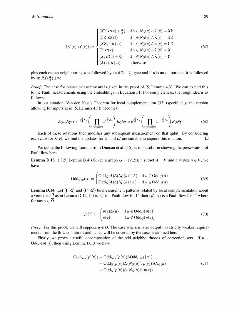
W. Simmons 89
(λ ′(v),α ′(v)) :=
(XY,α(v)+ π2) if v ∈ NG(u)∧λ (v) = XY
(Y Z,α(v)) if v ∈ NG(u)∧λ (v) = XZ
(XZ,−α(v)) if v ∈ NG(u)∧λ (v) = Y Z
(Y,α(v)) if v ∈ NG(u)∧λ (v) = X
(X ,α(v)+π) if v ∈ NG(u)∧λ (v) = Y
(λ (v),α(v)) otherwise
(67)
plus each output neighbouring u is followed by an RZ(−π2) gate and if u is an output then it is followed
by an RX(π2) gate.
Proof. The case for planar measurements is given in the proof of [5, Lemma 4.3]. We can extend this
to the Pauli measurements using the embeddings in Equation 51. For completeness, the rough idea is as
follows:
In our notation, Van den Nest’s Theorem for local complementation [33] (specifically, the version
allowing for inputs as in [5, Lemma 4.3]) becomes:
EG⋆uNI ≈ e−i
π4
Xu
(
∏w∈NG(u)
eiπ4
Zw
)
EGNI ≈ eiπ4
Xu
(
∏w∈NG(u)
e−i
π4
Zw
)
EGNI (68)
Each of these rotations then modifies any subsequent measurement on that qubit. By considering
each case for λ (v), we find the updates for λ ′ and α ′ are suitable to capture this rotation.
We quote the following Lemma from Duncan et al. [15] as it is useful in showing the preservation of
Pauli flow here.
Lemma D.13. ( [15, Lemma B.4]) Given a graph G = (V,E), a subset A ⊆ V and a vertex u ∈ V , we
have
OddG⋆u(A) =
{
OddG(A)∆(NG(u)∩A) if u /∈ OddG(A)
OddG(A)∆(NG(u)\A) if u ∈ OddG(A)(69)
Lemma D.14. Let (Γ,α) and (Γ′,α ′) be measurement patterns related by local complementation about
a vertex u ∈ I as in Lemma D.12. If (p,≺) is a Pauli flow for Γ, then (p′,≺) is a Pauli flow for Γ′ where
for any v ∈ O
p′(v) :=
{
p(v)∆{u} if u ∈ OddG(p(v))
p(v) if u /∈ OddG(p(v))(70)
Proof. For this proof, we will suppose u ∈ O. The case where u is an output has strictly weaker require-
ments from the flow conditions and hence will be covered by the cases examined here.
Firstly, we prove a useful decomposition of the odd neighbourhoods of correction sets. If u ∈OddG(p(v)), then using Lemma D.13 we have
OddG⋆u(p′(v)) = OddG⋆u(p(v))∆OddG⋆u({u})= OddG(p(v))∆(NG(u)\ p(v))∆NG(u)
= OddG(p(v))∆(NG(u)∩ p(v))
(71)
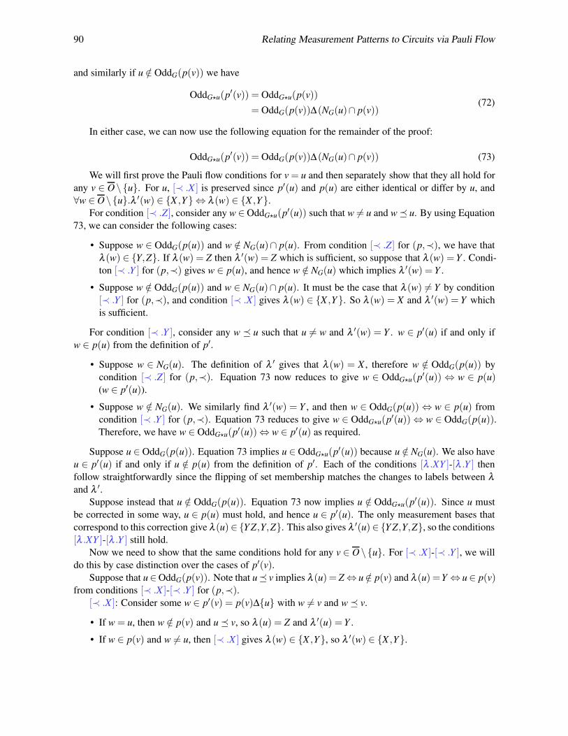
90 Relating Measurement Patterns to Circuits via Pauli Flow
and similarly if u /∈ OddG(p(v)) we have
OddG⋆u(p′(v)) = OddG⋆u(p(v))
= OddG(p(v))∆(NG(u)∩ p(v))(72)
In either case, we can now use the following equation for the remainder of the proof:
OddG⋆u(p′(v)) = OddG(p(v))∆(NG(u)∩ p(v)) (73)
We will first prove the Pauli flow conditions for v = u and then separately show that they all hold for
any v ∈ O\{u}. For u, [≺ .X ] is preserved since p′(u) and p(u) are either identical or differ by u, and
∀w ∈ O\{u}.λ ′(w) ∈ {X ,Y} ⇔ λ (w) ∈ {X ,Y}.
For condition [≺ .Z], consider any w ∈ OddG⋆u(p′(u)) such that w 6= u and w � u. By using Equation
73, we can consider the following cases:
• Suppose w ∈ OddG(p(u)) and w /∈ NG(u)∩ p(u). From condition [≺ .Z] for (p,≺), we have that
λ (w) ∈ {Y,Z}. If λ (w) = Z then λ ′(w) = Z which is sufficient, so suppose that λ (w) =Y . Condi-
ton [≺ .Y ] for (p,≺) gives w ∈ p(u), and hence w /∈ NG(u) which implies λ ′(w) = Y .
• Suppose w /∈ OddG(p(u)) and w ∈ NG(u)∩ p(u). It must be the case that λ (w) 6= Y by condition
[≺ .Y ] for (p,≺), and condition [≺ .X ] gives λ (w) ∈ {X ,Y}. So λ (w) = X and λ ′(w) = Y which
is sufficient.
For condition [≺ .Y ], consider any w � u such that u 6= w and λ ′(w) = Y . w ∈ p′(u) if and only if
w ∈ p(u) from the definition of p′.
• Suppose w ∈ NG(u). The definition of λ ′ gives that λ (w) = X , therefore w /∈ OddG(p(u)) by
condition [≺ .Z] for (p,≺). Equation 73 now reduces to give w ∈ OddG⋆u(p′(u)) ⇔ w ∈ p(u)(w ∈ p′(u)).
• Suppose w /∈ NG(u). We similarly find λ ′(w) = Y , and then w ∈ OddG(p(u)) ⇔ w ∈ p(u) from
condition [≺ .Y ] for (p,≺). Equation 73 reduces to give w ∈ OddG⋆u(p′(u)) ⇔ w ∈ OddG(p(u)).Therefore, we have w ∈ OddG⋆u(p′(u))⇔ w ∈ p′(u) as required.
Suppose u ∈ OddG(p(u)). Equation 73 implies u ∈ OddG⋆u(p′(u)) because u /∈ NG(u). We also have
u ∈ p′(u) if and only if u /∈ p(u) from the definition of p′. Each of the conditions [λ .XY ]-[λ .Y ] then
follow straightforwardly since the flipping of set membership matches the changes to labels between λ
and λ ′.Suppose instead that u /∈ OddG(p(u)). Equation 73 now implies u /∈ OddG⋆u(p′(u)). Since u must
be corrected in some way, u ∈ p(u) must hold, and hence u ∈ p′(u). The only measurement bases that
correspond to this correction give λ (u)∈{Y Z,Y,Z}. This also gives λ ′(u)∈{Y Z,Y,Z}, so the conditions
[λ .XY ]-[λ .Y ] still hold.
Now we need to show that the same conditions hold for any v ∈ O\{u}. For [≺ .X ]-[≺ .Y ], we will
do this by case distinction over the cases of p′(v).Suppose that u∈OddG(p(v)). Note that u� v implies λ (u) = Z ⇔ u /∈ p(v) and λ (u) =Y ⇔ u∈ p(v)
from conditions [≺ .X ]-[≺ .Y ] for (p,≺).[≺ .X ]: Consider some w ∈ p′(v) = p(v)∆{u} with w 6= v and w � v.
• If w = u, then w /∈ p(v) and u � v, so λ (u) = Z and λ ′(u) =Y .
• If w ∈ p(v) and w 6= u, then [≺ .X ] gives λ (w) ∈ {X ,Y}, so λ ′(w) ∈ {X ,Y}.

W. Simmons 91
[≺ .Z]: Consider some w ∈ OddG⋆u(p′(v)) = OddG(p(v))∆(NG(u)∩ p(v)) with w 6= v and w � v.
• If w = u then u � v, so λ (w) ∈ {Y,Z} and λ ′(w) ∈ {Y,Z}.
• If w ∈ OddG(p(v)), w 6= u, and w /∈ NG(u) ∩ p(v) then by [≺ .Z] we have λ (w) ∈ {Y,Z}. If
λ (w) = Z then λ ′(w) = Z. If λ (w) = Y , then w ∈ p(v) by [≺ .Y ], so w /∈ NG(u) by Equation 73
and therefore λ ′(w) = Y .
• If w /∈ OddG(p(v)) and w ∈ NG(u)∩ p(v), then by [≺ .X ] and [≺ .Y ] we must have λ (w) = X , so
λ ′(w) = Y .
[≺ .Y ]: Consider any w � v with w 6= v and λ ′(w) = Y .
• If w ∈ NG(u), then λ (w) = X and w 6= u. Using [≺ .Z] we get w /∈ OddG(p(v)), so Equation 73
reduces to w ∈ OddG⋆u(p′(v)) if and only if w ∈ p(v). Since w 6= u, this happens if and only if
w ∈ p′(v) = p(v)∆{u}.
• If w = u, then λ (w) = Z. By [≺ .X ] we have u /∈ p(v) and by assumption u ∈ OddG(p(v)). These
mean u ∈ p′(v) = p(v)∆{u} and u ∈ OddG⋆u(p′(v)) by Equation 73.
• If w /∈ NG(u) and w 6= u, then λ (w) = Y . Equation 73 gives w ∈ OddG⋆u(p′(v)) if and only if
w ∈ OddG(p(v)). Using [≺ .Y ], this happens if and only if w ∈ p(v) and thus if and only if w ∈p′(v) = p(v)∆{u}.
Otherwise, suppose u /∈ OddG(p(v)).[≺ .X ]: Consider some w ∈ p′(v) = p(v) with w 6= v and w � v.
• If w = u, then by [≺ .X ] and [≺ .Y ] we have λ (u) = X = λ ′(w).
• If w 6= u, then by [≺ .X ] we have λ (w) ∈ {X ,Y}, so λ ′(w) ∈ {X ,Y}.
[≺ .Z]: Consider some w ∈ OddG⋆u(p′(v)) = OddG(p(v))∆(NG(u)∩ p(v)) with w 6= v and w � v.
Since u /∈ NG(u) and u /∈ OddG(p(v)), w 6= u.
• If w ∈ NG(u), then Equation 73 gives w ∈ OddG(p(v))∆p(v). Conditions [≺ .X ]-[≺ .Y ] imply that
λ (w) ∈ {X ,Z}, so λ ′(w) ∈ {Y,Z}.
• If w /∈ NG(u), w ∈ OddG(p(v)) and λ ′(w) = λ (w), so the result follows straightforwardly from
[≺ .Z] for (p,≺).
[≺ .Y ]: Consider any w � v with w 6= v and λ ′(w) = Y .
• If w = u, then λ (u) = Z. From [≺ .X ], u /∈ p(v) = p′(v), and u /∈ OddG⋆u(p′(v)) since u /∈OddG(p(v)) by assumption and u /∈ NG(u).
• If w ∈ NG(u), then λ (w) = X . From [≺ .Z], w /∈ OddG(p(v)). Equation 73 then reduces to w ∈OddG⋆u(p′(v)) if and only if w ∈ p(v) = p′(v).
• If w /∈ NG(u) and w 6= u, then λ (w) = Y . Equation 73 gives w ∈ OddG⋆u(p′(v)) if and only if
w ∈ OddG(p(v)), which happens if and only if w ∈ p(v) = p′(v) by [≺ .Y ] for (p,≺).
[λ .XY ]-[λ .Y Z]: Suppose λ (v) ∈ {XY,XZ,YZ}. Since v ∈ O\{u}, v ∈ p′(v) if and only if v ∈ p(v).Whether or not v ∈ p(v) and v ∈ Odd(p(v)) is given by [λ .XY ]-[λ .Y Z] for (p,≺) and the value of λ (v).
• If v ∈ NG(u), then Equation 73 gives v ∈ OddG⋆u(p′(v)) if and only if v ∈ OddG(p(v))∆p(v). This
change in the odd neighbourhood coincides with the definition of λ ′ flipping the labels of XZ and
Y Z.

92 Relating Measurement Patterns to Circuits via Pauli Flow
• If v /∈ NG(u), then Equation 73 gives v ∈ OddG⋆u(p′(v)) if and only if v ∈ OddG(p(v)), which is
enough since λ ′(v) = λ (v).
[λ .X ]-[λ .Y ]: We will prove these conditions by considering the possible cases for λ (v) ∈ {X ,Y,Z}in turn. In each case, since v 6= u, v ∈ p′(v) if and only if v ∈ p(v).
If λ (v) = Z, then λ ′(v) = Z and we get v ∈ p(v) (v ∈ p′(v)) from [λ .Z] for (p,≺).Suppose λ (v) = X , so v ∈ OddG(p(v)) from [λ .X ] for (p,≺).
• If v ∈ NG(u), then λ ′(v) = Y and Equation 73 gives v ∈ OddG⋆u(p′(v)) if and only if v /∈ p(v)(v /∈ p′(v)).
• If v /∈ NG(u), then λ ′(v) = X and Equation 73 gives v ∈ OddG⋆u(p′(v)).
Suppose λ (v) = Y , so v ∈ p(v)⇔ v /∈ OddG(p(v)) from [λ .Y ] for (p,≺).
• If v ∈ NG(u), then λ ′(v) = X . Since v ∈ OddG(p(v))∆p(v), Equation 73 gives v ∈ OddG⋆u(p′(v)).
• If v /∈ NG(u), then λ ′(v) = Y . Equation 73 gives v ∈ OddG⋆u(p′(v)) if and only if v ∈ OddG(p(v)).From [λ .Y ] and v 6= u, this happens if and only if v /∈ p′(v).
Lemma D.15. Let (Γ,α) and (Γ′,α ′) be the measurement patterns from Lemma D.12 related by local
complementation about a vertex u ∈ I. If (p,≺) is a focussed Pauli flow for Γ, then (p′,≺) is a focussed
pauli flow for Γ′, where p′ is defined in ≻-order (from outputs backwards) as
p′(v) :=
{
p(v)∆{u} if u ∈ OddG(p(v))p(v) if u /∈ OddG(p(v))
}
∆ ∆w∈O\{v}
w∈p(v)∪OddG(p(v))w∈NG(u)∪{u}
w∈NG(u)⇒λ(w)=XYw=u⇒λ(u)/∈{X ,Y,Z}
p′(w) (74)
Furthermore, if p̂ is a focussed set for Γ, then we obtain a corresponding focussed set for Γ′ as
p̂′ :=
{
p̂∆{u} if u ∈ OddG(p̂)p̂ if u /∈ OddG(p̂)
}
∆ ∆w∈O
w∈p̂∪OddG( p̂)w∈NG(u)∪{u}
w∈NG(u)⇒λ(w)=XYw=u⇒λ(u)/∈{X ,Y,Z}
p′(w) (75)
Proof. Lemma D.14 gives a Pauli flow for Γ′, which we will rename as (q,≺). We can view (q,≺) as
an intermediate in the construction of (p′,≺). It is not necessarily focussed, but we can refocus it using
Lemma 4.6. Recall that this adds correction sets together according to Lemma B.1 for any case where the
focussed conditions do not hold for q. We just need to show that these cases match those in the definition
of p′.As usual, the proofs for Pauli flows and focussed sets are almost identical, so herein we could change
out references of q for
q̂ :=
{
p̂∆{u} if u ∈ OddG(p̂)
p̂ if u /∈ OddG(p̂)(76)
as an intermediate in the construction of p̂′.
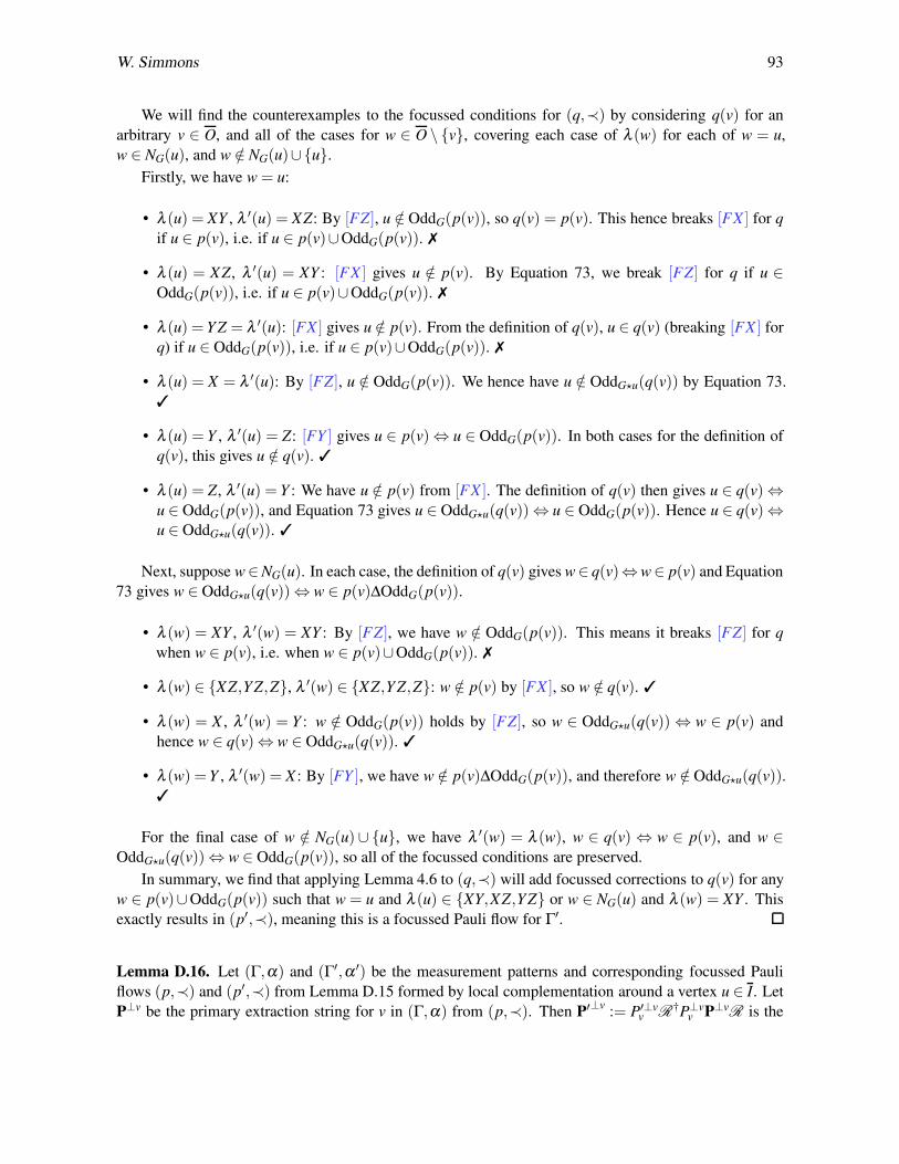
W. Simmons 93
We will find the counterexamples to the focussed conditions for (q,≺) by considering q(v) for an
arbitrary v ∈ O, and all of the cases for w ∈ O \ {v}, covering each case of λ (w) for each of w = u,
w ∈ NG(u), and w /∈ NG(u)∪{u}.
Firstly, we have w = u:
• λ (u) = XY , λ ′(u) = XZ: By [FZ], u /∈ OddG(p(v)), so q(v) = p(v). This hence breaks [FX ] for q
if u ∈ p(v), i.e. if u ∈ p(v)∪OddG(p(v)). ✗
• λ (u) = XZ, λ ′(u) = XY : [FX ] gives u /∈ p(v). By Equation 73, we break [FZ] for q if u ∈OddG(p(v)), i.e. if u ∈ p(v)∪OddG(p(v)). ✗
• λ (u) = Y Z = λ ′(u): [FX ] gives u /∈ p(v). From the definition of q(v), u ∈ q(v) (breaking [FX ] for
q) if u ∈ OddG(p(v)), i.e. if u ∈ p(v)∪OddG(p(v)). ✗
• λ (u) = X = λ ′(u): By [FZ], u /∈ OddG(p(v)). We hence have u /∈ OddG⋆u(q(v)) by Equation 73.
✓
• λ (u) = Y , λ ′(u) = Z: [FY ] gives u ∈ p(v)⇔ u ∈ OddG(p(v)). In both cases for the definition of
q(v), this gives u /∈ q(v). ✓
• λ (u) = Z, λ ′(u) = Y : We have u /∈ p(v) from [FX ]. The definition of q(v) then gives u ∈ q(v) ⇔u ∈ OddG(p(v)), and Equation 73 gives u ∈ OddG⋆u(q(v))⇔ u ∈ OddG(p(v)). Hence u ∈ q(v)⇔u ∈ OddG⋆u(q(v)). ✓
Next, suppose w∈NG(u). In each case, the definition of q(v) gives w∈ q(v)⇔w∈ p(v) and Equation
73 gives w ∈ OddG⋆u(q(v))⇔ w ∈ p(v)∆OddG(p(v)).
• λ (w) = XY , λ ′(w) = XY : By [FZ], we have w /∈ OddG(p(v)). This means it breaks [FZ] for q
when w ∈ p(v), i.e. when w ∈ p(v)∪OddG(p(v)). ✗
• λ (w) ∈ {XZ,YZ,Z}, λ ′(w) ∈ {XZ,Y Z,Z}: w /∈ p(v) by [FX ], so w /∈ q(v). ✓
• λ (w) = X , λ ′(w) = Y : w /∈ OddG(p(v)) holds by [FZ], so w ∈ OddG⋆u(q(v)) ⇔ w ∈ p(v) and
hence w ∈ q(v)⇔ w ∈ OddG⋆u(q(v)). ✓
• λ (w) =Y , λ ′(w) = X : By [FY ], we have w /∈ p(v)∆OddG(p(v)), and therefore w /∈ OddG⋆u(q(v)).✓
For the final case of w /∈ NG(u)∪ {u}, we have λ ′(w) = λ (w), w ∈ q(v) ⇔ w ∈ p(v), and w ∈OddG⋆u(q(v))⇔ w ∈ OddG(p(v)), so all of the focussed conditions are preserved.
In summary, we find that applying Lemma 4.6 to (q,≺) will add focussed corrections to q(v) for any
w ∈ p(v)∪OddG(p(v)) such that w = u and λ (u) ∈ {XY,XZ,YZ} or w ∈ NG(u) and λ (w) = XY . This
exactly results in (p′,≺), meaning this is a focussed Pauli flow for Γ′.
Lemma D.16. Let (Γ,α) and (Γ′,α ′) be the measurement patterns and corresponding focussed Pauli
flows (p,≺) and (p′,≺) from Lemma D.15 formed by local complementation around a vertex u ∈ I. Let
P⊥v be the primary extraction string for v in (Γ,α) from (p,≺). Then P′⊥v:= P′⊥v
v R†P⊥vv P⊥vR is the
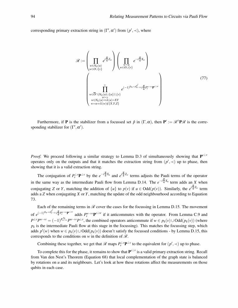
94 Relating Measurement Patterns to Circuits via Pauli Flow
corresponding primary extraction string in (Γ′,α ′) from (p′,≺), where
R :=
∏w∈NG(u)w∈O∪{v}
eiπ4
Zw
∏w=u
w∈O∪{v}
e−i
π4
Xw
≻∏
w∈O∩(NG(u)∪{u})\{v}w≻v
w∈NG(u)⇒λ(u)=XY
w=u⇒λ(w)/∈{X ,Y,Z}
e(−1)Dw+A
p′w→v i
π4
Pw→vv P′⊥w
(77)
Furthermore, if P is the stabilizer from a focussed set p̂ in (Γ,α), then P′ := R†PR is the corre-
sponding stabilizer for (Γ′,α ′).
Proof. We proceed following a similar strategy to Lemma D.3 of simultaneously showing that P′⊥v
operates only on the outputs and that it matches the extraction string from (p′,≺) up to phase, then
showing that it is a valid extraction string.
The conjugation of P⊥vv P⊥v by the e
−iπ4
Xu and eiπ4
Zw terms adjusts the Pauli terms of the operator
in the same way as the intermediate Pauli flow from Lemma D.14. The e−i
π4
Xu term adds an X when
conjugating Z or Y , matching the addition of {u} to p(v) if u ∈ Odd(p(v)). Similarly, the eiπ4
Zw term
adds a Z when conjugating X or Y , matching the update of the odd neighbourhood according to Equation
73.
Each of the remaining terms in R cover the cases for the focussing in Lemma D.15. The movement
of e(−1)Dw+A
p′w→v i
π4
Pw→vv P′⊥w
adds Pw→vv P′⊥w
if it anticommutes with the operator. From Lemma C.9 and
P⊥vPw→v = (−1)Fpk
w→v Pw→vP⊥v, the combined operators anticommute if w ∈ pk(v)∪Odd(pk(v)) (where
pk is the intermediate Pauli flow at this stage in the focussing). This matches the focussing step, which
adds p′(w) when w ∈ pk(v)∪Odd(pk(v)) doesn’t satisfy the focussed conditions - by Lemma D.15, this
corresponds to the conditions on w in the definition of R.
Combining these together, we get that R maps P⊥vv P⊥v to the equivalent for (p′,≺) up to phase.
To complete this for the phase, it remains to show that P′⊥vis a valid primary extraction string. Recall
from Van den Nest’s Theorem (Equation 68) that local complementation of the graph state is balanced
by rotations on u and its neighbours. Let’s look at how these rotations affect the measurements on those
qubits in each case.

W. Simmons 95
λ (w) w = u w ∈ NG(u)
XY 〈+XZ,
π2|ei
π4
X= 〈+XY,0| 〈+XY,
π2|e−i
π4
Z≈ 〈+XY,0|
XZ 〈+XY,
π2|ei
π4
X≈ 〈+XZ,0| 〈+YZ,0|e−iπ4
Z≈ 〈+XZ,0|
Y Z 〈+YZ,
π2|ei
π4
X= 〈+YZ,0| 〈+XZ,0|e−iπ4
Z≈ 〈+YZ,0|
X 〈+X ,α(w)|eiπ4
X≈ 〈+X ,α(w)| 〈+Y,α(w)|e−iπ4
Z≈ 〈+X ,α(w)|Y 〈+Z,α(w)+π |ei
π4
X≈ 〈+Y,α(w)| 〈+X ,α(w)+π |e−iπ4
Z≈ 〈+Y,α(w)|Z 〈+Y,α(w)|ei
π4
X≈ 〈+Z,α(w)| 〈+Z,α(w)|e−iπ4
Z≈ 〈+Z,α(w)|
We can now consider the primary extraction string of some v ∈ O. As usual, we define C ′ to be the
linear map of interest from Definition 4.2 for (Γ′,α ′) and let C refer to the equivalent for (Γ,α).
C′ :=
∏w≻v
λ ′(w)/∈{X ,Y,Z}
〈+λ ′(w),0|w
∏w∈O\{v}
λ ′(w)∈{X ,Y,Z}
〈+λ ′(w),α ′(w)|w
EG⋆uNI (78)
We start by applying the reverse of the extraction algorithm to modify the measurement angles in the
diagram to match those in the table above. Since this changes the angles (which must be 0 to extract any
rotation before them), we must perform this in ≺-order.
C′ ≈
∏w≻v
w∈NG(u)∪{u}w∈NG(u)⇒λ ′(w)=XY
w=u⇒λ ′(w)/∈{X ,Y,Z}
〈+λ ′(w),π
2|w
e(−1)1+Dw i
π4
P⊥ww
∏w≻vw6=u
w∈NG(u)⇒λ ′(w)∈{XZ,Y Z}w/∈NG(u)⇒λ ′(w)/∈{X ,Y,Z}
〈+λ ′(w),0|w
∏w∈O\{v}
λ ′(w)∈{X ,Y,Z}
〈+λ ′(w),α ′(w)|w
EG⋆uNI
=
≺∏w≻v
w∈NG(u)∪{u}w∈NG(u)⇒λ ′(w)=XY
w=u⇒λ ′(w)/∈{X ,Y,Z}
e(−1)1+Dw+A
p′w→v i
π4
Pw→vv P′⊥w
∏w≻v
w∈NG(u)∪{u}w∈NG(u)⇒λ ′(w)=XY
w=u⇒λ ′(w)/∈{X ,Y,Z}
〈+λ ′(w),π
2|w
∏w≻vw6=u
w∈NG(u)⇒λ ′(w)∈{XZ,Y Z}w/∈NG(u)⇒λ ′(w)/∈{X ,Y,Z}
〈+λ ′(w),0|w
∏w∈O\{v}
λ ′(w)∈{X ,Y,Z}
〈+λ ′(w),α ′(w)|w
EG⋆uNI
(79)

96 Relating Measurement Patterns to Circuits via Pauli Flow
Next, we apply Van den Nest’s Theorem to yield C .
C′ ≈
≺∏w≻v
w∈NG(u)∪{u}w∈NG(u)⇒λ ′(w)=XY
w=u⇒λ ′(w)/∈{X ,Y,Z}
e(−1)1+Dw+A
p′w→v i
π4
Pw→vv P′⊥w
∏w≻v
w∈NG(u)∪{u}w∈NG(u)⇒λ ′(w)=XY
w=u⇒λ ′(w)/∈{X ,Y,Z}
〈+λ ′(w),π
2|w
∏w≻vw6=u
w∈NG(u)⇒λ ′(w)∈{XZ,Y Z}w/∈NG(u)⇒λ ′(w)/∈{X ,Y,Z}
〈+λ ′(w),0|w
∏w∈O\{v}
λ ′(w)∈{X ,Y,Z}
〈+λ ′(w),α ′(w)|w
eiπ4
Xu
(
∏w∈NG(u)
e−i
π4
Zw
)
EGNI
≈
≺∏w≻v
w∈NG(u)∪{u}w∈NG(u)⇒λ ′(w)=XY
w=u⇒λ ′(w)/∈{X ,Y,Z}
e(−1)1+Dw+A
p′w→v i
π4
Pw→vv P′⊥w
∏w=u
w∈O∨w�v
w∈O\{v}⇒λ(w)/∈{X ,Y,Z}
eiπ4
Xw
∏w∈NG(u)
w∈O∨w�v
w∈O\{v}⇒λ(w)/∈{X ,Y,Z}
e−i
π4
Zw
∏w≻v
λ(w)/∈{X ,Y,Z}
〈+λ(w),0|w
∏w∈O\{v}
λ(w)∈{X ,Y,Z}
〈+λ(w),α(w)|w
EGNI
= R†
∏w=u6=v
w�vλ(w)/∈{X ,Y,Z}
eiπ4
Xw
∏w∈O∩NG(u)\{v}
w�vλ(w)/∈{X ,Y,Z}
e−i
π4
Zw
C
(80)

W. Simmons 97
The final step is then to introduce P⊥vv P⊥v, move it through R and reverse the construction to return
to C ′.
C′ ≈ R
†
∏w=u6=v
w�vλ(w)/∈{X ,Y,Z}
eiπ4
Xw
∏w∈O∩NG(u)\{v}
w�vλ(w)/∈{X ,Y,Z}
e−i
π4
Zw
P⊥vP⊥vv C
= P′⊥vP′⊥v
v R†
∏w=u6=v
w�vλ(w)/∈{X ,Y,Z}
eiπ4
Xw
∏w∈O∩NG(u)\{v}
w�vλ(w)/∈{X ,Y,Z}
e−i
π4
Zw
C
≈ P′⊥vP′⊥v
v C′
(81)
Hence P′⊥vis a valid primary extraction string for v, and by Lemma C.8 it is exactly the one generated
by (p′,≺). As usual, the proof is virtually identical for stabilizers from focussed sets.
Theorem D.17. (Restatement of Theorem 5.3) Performing local complementation about a vertex u cor-
responds to the following sequence of actions on the PDDAG:
1. For each output w neighbouring u, a (Zw,π2) rotation is pulled from the initial stabilizer block all
the way to the end of the rotation DAG;
2. If u is an output, a (Xu,−π2) rotation is pulled from the initial stabilizer block all the way to the
end of the rotation DAG;
3. For each vertex w neighbouring u with λ (w) = XY , and for u itself if λ (u) is planar, we pull a(
P′⊥w,(−1)Dw π2
)
rotation from the initial stabilizer block to merge it into the existing rotation for
w or u. We do this in ≻-order over such w vertices.
Proof. Lemma D.12 shows that the additions of π2
to measurement angles and outputs matches the set of
rotations that are moved in the above PDDAG rewrite sequence.
The updates for the Pauli strings for each rotation and the stabilizers/tableau are covered by Lemma
D.16. In particular, in each case we consider planar vertices and so all of the Pw→vv terms in R are I,
meaning the update to the extraction string corresponds to the effect of the Reorder Rules. However, the
phase may differ in the update from P⊥v to P′⊥v.
P⊥v eiπ4
XvP⊥ve−i
π4
Xv e−i
π4
Zv P⊥veiπ4
Zv
X X Y
Y −Z −X
Z Y Z
This shows that we experience an extra phase flip in the extraction string for u when λ (v) = XZ,
balanced by the negating of α(u) in the statement of Lemma D.12. For v ∈ NG(u), we get an extra phase
flip for λ (v) ∈ {XZ,YZ} from Equation 10, which cancels with the above for λ (v) = XZ and is balanced
by the negating of α(v) when λ (v) =Y Z.

98 Relating Measurement Patterns to Circuits via Pauli Flow
Example D.18. Again, we start from the same measurement pattern from Example C.13 and apply local
complementation about vertex d. This complements the connectivity within {a,b,c,o2}.
i d
a
o2
c o1
b
v λ ′(v) α ′(v) p′(v) Odd(p′(v)) {u|v ≺ u}i XY α(i) b,c,o2 i,a,d,o1 a,b,c,o1,o2
a XZ −α(a) a,c,o1,o2 a,d,o1 c,o1,o2
b XY α(b)+ π2
c b,d,o1,o2 c,o1,o2
c XY α(c)+ π2
o1 c o1
d Z α(d)+π d,o2 d,o2 o2
We update the focussed set p̂ to p̂′ = {c,o1,o2}, and to preserve semantics we also have an RZ(−π2)
applied to output o2.
Now we turn to the sequence of rewrites on the PDDAG. For step 1, o2 neighbours d so we pull
a (I1Z2,π2) rotation through to the end. The Reorder Rules update the rotations with anticommuting
Pauli strings (the rotation from a, the tableau row and rotation from i, and the free stabilizer from p̂) by
multiplication.
Ins Outs Sign
X Y Z (−)ad+1
Z Y +
Z Y +
(I1Y2,α(i)) ((−1)ad+1Z1X2,α(a)) (I1Z2,π2)
((−1)ad+1Y1Z2,α(b)) (X1I2,α(c))
Step 2 does not apply since d is not an output. Finally, in step 3, d is not planar but it is adjacent to b
and c that are labelled as XY . Since b ≺ c, we first pull out the (X1I2,π2) rotation.
Ins Outs Sign
X Z Z (−)ad+1
Z Y +
Y Y −
(I1Y2,α(i)) ((−1)adY1X2,α(a)) (I1Z2,π2)
((−1)ad+1Z1Z2,α(b)) (X1I2,α(c)+ π2)
Then we pull out the ((−1)ad+1Z1Z2,π2) rotation for b.
Ins Outs Sign
X Z Z (−)ad+1
Z Z X (−)ad
Y Y −
((−1)ad Z1X2,α(i)) ((−1)adY1X2,α(a)) (I1Z2,π2)
((−1)ad+1Z1Z2,α(b)+ π2) (X1I2,α(c)+ π
2)
We now find that this is the same PDDAG that would be extracted after applying the local comple-
mentation on the measurement pattern (take care when determining the phases during extraction as the
phase from including d in p′(v)∪Odd(p′(v)) is now (−1)ad+1 because α ′(d) = α(d)+π). In the final
step, it is important to have maintained the convention of extracting as ((−1)Dv P⊥v,α(v)) and keeping
the −1 terms with the string rather than the angle. If we had instead moved ((−1)ad Z1Z2,−π2), we would
end up with a rotation of α(b)− π2
and different phases on the rotation and tableau row for i.
Remark D.19. One should note that the action of local complementation is not quite self-inverse due to
some measurement angles being updated by π2
. However, performing the inverse update is also valid and
just relies on using the other case of Equation 68 to flip the angles that are added. This can similarly be
simulated by just flipping the angles of the rotations being moved through the PDDAG.
Now that we have the ability to simulate the effects of local complementation, extending this to
pivoting is trivial since it simply decomposes into a sequence of local complementations.

W. Simmons 99
Definition D.20. Given a graph G = (V,E) with some designated edge u ∼ v ∈ E , the pivot of G about
the edge u ∼ v is the operation resulting in the graph:
G∧uv := G⋆u⋆ v⋆u(= G⋆ v⋆u⋆ v) (82)
Lemma D.21. Let (Γ,α) describe a measurement pattern with Γ = (G, I,O,λ ) and some chosen vertices
u,v ∈ I such that u ∼ v. Then performing a pivot around the edge u ∼ v gives an equivalent measurement
pattern (Γ′,α ′) where Γ′ = (G∧uv, I,O, λ̂ ), for all a ∈ {u,v} and w ∈ O\{u,v}
(λ ′(a),α ′(a)) :=
(Y Z,−α(a)) if λ (a) = XY
(XZ, π2−α(a)) if λ (a) = XZ
(XY,−α(a)) if λ (a) =Y Z
(Z,α(a)) if λ (a) = X
(Y,α(a)+π) if λ (a) =Y
(X ,α(a)) if λ (a) = Z
(83)
(λ ′(w),α ′(w)) :=
(λ (w),α(w)+π) if w ∈ NG(u)∩NG(v)∧λ (w) ∈ {XY,X ,Y}(λ (w),−α(w)) if w ∈ NG(u)∩NG(v)∧λ (w) ∈ {XZ,Y Z}(λ (w),α(w)) otherwise
(84)
plus each output neighbouring both u and v is followed by a Z gate and if each of u or v is an output then
it is followed by a Hadamard gate.
Proof. We can similarly extend the case for planar measurements given in the proof of [5, Lemma 4.5]
to Pauli measurements by considering how they embed into the planes as in Equation 51. Similarly, this
follows by using Van den Nest’s Theorem [33] (Equation 68) multiple times, alternating the phases of
the angles each time, and rotating the measurement projections accordingly.
Since this proof requires alternating between the different phase variants of Equation 68, simulating
the effect in the PDDAG requires alternating between the different variants of local complementation as
mentioned in Remark D.19 but is otherwise just a trivial application of Theorem 5.3.
D.4 Alternative Focussed Pauli Flows
Lemma D.22. Let (Γ,α) describe a measurement pattern with a focussed set p̂, vertex v ∈ O, and two
focussed Pauli flows (p,≺) and (p′,≺) related by the addition of p̂ to p(v) as in Lemma B.6. Let P̂ be
the stabilizer corresponding to p̂, and P⊥v and P′⊥vbe the primary extraction strings for v according to
(p,≺) and (p′,≺′) respectively. Then P′⊥v = P⊥vP̂.
Proof. Lemma C.7 immediately gives this result up to phase. To invoke Lemma C.8, we consider the
linear map C for extraction strings of v. From the conditions of Lemma B.6 and the definition of ≺′,any w ∈ p̂∪Odd(p̂) must satisfy w 6= v and λ (w) /∈ {X ,Y,Z} ⇒ v ≺ w. So both P⊥v
v P⊥v and P̂ are
stabilizers of C , meaning they combine to give the stabilizer P⊥vv P⊥vP̂ which defines this as a valid
primary extraction string.

100 Relating Measurement Patterns to Circuits via Pauli Flow
Theorem D.23. (Restatement of Theorem 5.4) Let (Γ,α) describe a measurement pattern with some
focussed Pauli flow (p,≺), a focussed set p̂, and some vertex u ∈ O such that ∀w ∈ p̂∪Odd(p̂).λ (w) ∈{XY,XZ,YZ} ⇒ w 6= u∧ u ≺ w. Updating p(u) to p(u)∆ p̂ corresponds to a free action on the isome-
try tableau if u is an input, and applying the Product Rotation Lemma to the rotation from u with the
stabilizer of p̂ if u has a planar label.
Therefore, any two focussed Pauli flows for the same labelled open graph yield PDDAGs that are
related by a sequence of applications of the Product Rotation Lemma and free actions on the isometry
tableau.
Proof. This update on the Pauli flow is the same as from Lemma B.6, meaning Lemma D.22 gives the
update to the primary extraction strings. For both uses of u in extraction, we assume u has a planar label.
If u is an input considered for the tableau of the PDDAG, multiplication of a row of the tableau by a
free stabilizer is a free action as it just gives another equivalent set of generators for the stabilizer group.
On the other hand, if u is some planar vertex giving a rotation in the PDDAG, we note that P̂ remains
a stabilizer after applying each of the rotations for vertices w � u (they commute according to Lemma
C.9), allowing us to apply the Product Rotation Lemma to get the same effect.
To show that any two focussed Pauli flows (p,≺) and (p′,≺′) can be related using this, we start with
(p,≺) and derive the sequence of transformations needed to reach (p′,≺′).We consider weakening of the partial order in a Pauli flow to be a free action, as well as the reverse
so long as the Pauli flow conditions are preserved, since neither affect the semantics or extraction. So
suppose wlog that ≺ and ≺′ are minimal, i.e. ≺ is the transitive closure of {(u,v)|v ∈ p(u)∪Odd(p(u))∧u 6= v∧λ (v) ∈ {XY,XZ,YZ}} (we ignore Pauli measurements by Lemma B.11).
We proceed inductively over ≺. Under some indexing of the vertices respecting ≺, let v be the
first for which p(v) 6= p′(v), i.e. ∀w ≺ v.p(v) = p′(v). Our assumptions on minimality then imply that
∀w ∈ O.w ≺ v ⇔ w ≺′ v.
By Lemma B.7, p̂v := p(v)∆p′(v) is a focussed set for any v ∈ O. Conditions [λ .XY ]-[λ .Y Z] imply
that λ (v) ∈ {XY,XZ,YZ} ⇒ v /∈ p̂v ∪Odd(p̂v). Using conditions [≺ .X ] and [≺ .Z], we also have ∀w ∈p̂v∪Odd(p̂v).w 6= v∧λ (w)∈ {XY,XZ,YZ}⇒ v≺w∨v≺′ w. Since v≺′ w⇒ v�′ w and v�′ w⇔ v�w
by the minimality assumption, we now have ∀w ∈ p̂v ∪Odd(p̂v).λ (w) ∈ {XY,XZ,YZ}⇒ w 6= v∧ v � w.
This means that combining (p,≺) with v̂ according to Lemma B.6 (and reducing to the minimal order)
gives a focussed Pauli flow equal to (p′,≺′) up to v in ≺.
Repeating this inductively over the remaining vertices will eventually yield (p′,≺′).
Example D.24. We revisit the measurement pattern from Example C.13. Recall that we have a focussed
set p̂ = {c,o2} with Odd(p̂) = {a,o1}, so we can freely add this to the correction sets for any of i, b, or
d. Suppose we do so for b and d to give the following focussed Pauli flow:
v λ (v) p′(v) Odd(p′(v)) {u|v ≺ u}i XY b,o2 i,a a,b,c,o1,o2
a Y Z a,c,d,o2 d,o1,o2 c,o1,o2
b XY d,o1,o2 a,b,d,o2 a,c,o1,o2
c XY o1 c o1
d Y c a,d,o1 a,c,o1,o2
The difference between p(d) and p′(d) has no effect on the PDDAG since d is not involved in the
extraction procedure. So the only rewrites needed are the multiplication of the top row of the isometry
tableau by the bottom, and applying the Product Rotation Lemma to the b rotation mapping Y1Z2 7→(Y1Z2)(Z1X2) =−X1Y2.
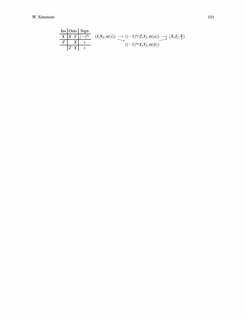
W. Simmons 101
Ins Outs Sign
X X Y (−)ad
Z X +
Z X +
(I1X2,α(i)) ((−1)ad Z1Y2,α(a)) (X1I2,π2)
((−1)ad X1Y2,α(b))