reinforcement learning approach to product allocation - drs1496/... · reinforcement learning...
TRANSCRIPT
Reinforcement Learning Approach to
Product Allocation and Storage
Masters Thesis Presented
By
Mitha Andra
To
Department of Industrial Engineering
In partial fulfillment of the requirements for the degree of
Masters of Science
In the field of
Industrial Engineering
Advisor
Sagar Kamarthi
Northeastern University
Boston, Massachusetts
May, 2010
i
Table of Contents
List of Figures ................................................................................................................................. ii
Acknowledgements ........................................................................................................................ iii
Abstract .......................................................................................................................................... iv
Chapter 1 ......................................................................................................................................... 1
1.1 Introduction .................................................................................................................. 1
1.2 Problem Statement ........................................................................................................ 8
1.3 Approach ...................................................................................................................... 9
Chapter 2 ....................................................................................................................................... 15
2.1 Literature Review ....................................................................................................... 15
2.2 Quadratic Assignment Problem .................................................................................. 20
Chapter 3 ....................................................................................................................................... 23
3.1 Reinforcement Learning ............................................................................................. 23
3.2 Application to Our Problem ....................................................................................... 27
Chapter 4 ....................................................................................................................................... 37
4.1 Concluding Remarks ................................................................................................... 37
References ..................................................................................................................................... 38
Appendix A. Notations ................................................................................................................. 44
Appendix A. Analysis ................................................................................................................... 45

ii
List of Figures
Figure 1.1 Layout of the warehouse ............................................................................................... 5
Figure 1.2 Bulk area layout with 14 sub-areas, 2 exits, and staging area ....................................... 6
Figure 1.3 Reinforcement learning model (4)............................................................................... 10
Figure 1.4 Q-Learning algoritm (5) .............................................................................................. 14
Figure 2.1 Warehouse design decision parameters (19) ............................................................... 17
Figure 3.1 Reinforcement learning architecture (50) .................................................................... 25
Figure 3.2 The structure of the learning system, with the agent, the environment, the agent
listeners as interface for the learning algorithms and agent controllers (13) ................................ 26
Figure 3.3 Reward matrix example ............................................................................................... 30
iii
Acknowledgements
Sincere gratitude is extended to Prof. Sagar Kamarthi, my thesis advisor, for his guidance and
support. In addition I would like to thank MS Walker, Inc. for providing the necessary data to
accomplish this thesis.
iv
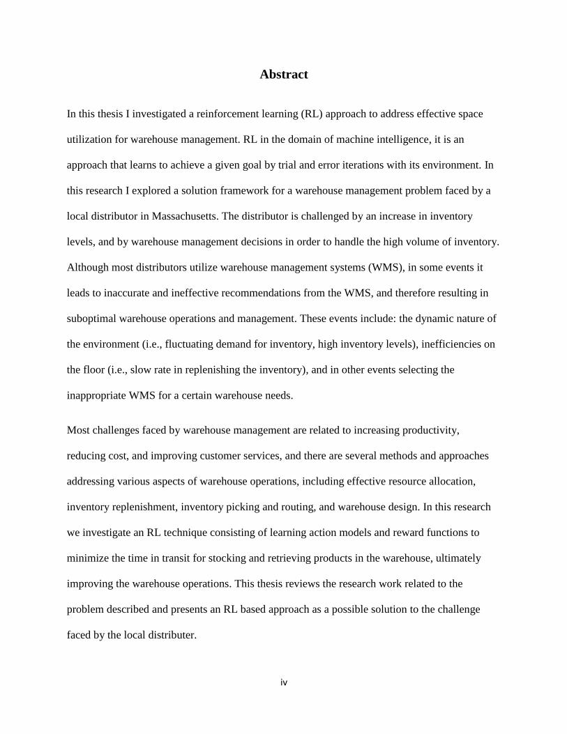
Abstract
In this thesis I investigated a reinforcement learning (RL) approach to address effective space
utilization for warehouse management. RL in the domain of machine intelligence, it is an
approach that learns to achieve a given goal by trial and error iterations with its environment. In
this research I explored a solution framework for a warehouse management problem faced by a
local distributor in Massachusetts. The distributor is challenged by an increase in inventory
levels, and by warehouse management decisions in order to handle the high volume of inventory.
Although most distributors utilize warehouse management systems (WMS), in some events it
leads to inaccurate and ineffective recommendations from the WMS, and therefore resulting in
suboptimal warehouse operations and management. These events include: the dynamic nature of
the environment (i.e., fluctuating demand for inventory, high inventory levels), inefficiencies on
the floor (i.e., slow rate in replenishing the inventory), and in other events selecting the
inappropriate WMS for a certain warehouse needs.
Most challenges faced by warehouse management are related to increasing productivity,
reducing cost, and improving customer services, and there are several methods and approaches
addressing various aspects of warehouse operations, including effective resource allocation,
inventory replenishment, inventory picking and routing, and warehouse design. In this research
we investigate an RL technique consisting of learning action models and reward functions to
minimize the time in transit for stocking and retrieving products in the warehouse, ultimately
improving the warehouse operations. This thesis reviews the research work related to the
problem described and presents an RL based approach as a possible solution to the challenge
faced by the local distributer.
1
Chapter 1
1.1 Introduction
The focus of warehouse operations is about ensuring the right quantity of the right product is
delivered to the right customer at the right time, and this requires the product to be picked and
dispatched from the warehouse in right quantity in a timely manner. Effective warehouse
operations are critical in product delivery and in maintaining good customer relations, especially
due to the numerous activities involved, an effective collaboration of these activities is required
to manage issues such as high inventory levels and transportation costs, and productivity levels.
The research presented in this thesis particularly focuses on the warehouse operation practices of
a local wholesale distributor of wines, spirits, and cigars. The distributor is challenged by
inefficient operations and by use of space in the Bulk storage area of the facility. In addition, the
distributor anticipates an increase in demand for the product base and would like to expand the
facility capacity to accommodate for this increase in inventory. Inefficient space utilization is a
major area of concern to the distributor; product inventories are stored in bulk to meet the
unpredictable customer demand. It is important to understand the cause for the high inventory
levels at the warehouse as it would provide insight into variables impacting and leading to
suboptimal warehouse operations. As in most cases, the distributor holds stock at various stages
within the supply chain due to factors such as, an unpredictable and irregular demand for product
type, incentives such as lower shipping costs per unit for larger orders and discounts in bulk
buying, safety stock to cover for lead time, and high seasonality.

2
The problem of effective space utilization and resource allocation is largely applicable to other
fields such as manufacturing production control, fleet management, and personnel management.
Researchers have examined and proposed solutions for various problem areas in warehouse
management such as inventory allocation involving single and multiple retailers, best methods
for shipment consolidation, optimal policy for production and inventory control, timing of
shipment and quantity for a certain product, approaches for coordination of shipment and stock
rebalancing, and optimizing inventory dispatching policies. Several solution methods have been
proposed with basis in, Artificial Intelligence (AI) methods [1], search algorithms [2];
reinforcement learning (RL) approaches [3].
Although several approaches have been explored, this problem continues to draw research and
efficient solution methods: for instance, a certain layout or storage assignment may prove to be
effective for certain routing strategies, but ineffective for others. Additionally, there are several
objectives and decisions that could be explored for effective space utilization and resource
allocation including maximizing criteria such as the use of equipment, labor, and use of space.
In this thesis we analyze the relationships among inventory type, ordering quantity and inventory
location, and apply reinforcement learning approach to manage inventory, and optimize space
allocation at the stock keeping unit (SKU)/store level by minimizing average travel distance.
Warehouse Operations
This section will discuss the conditions at the local distributor in Massachusetts. The product
arriving at the warehouse on any given day varies highly based on the product type, quantity, and
supplier. Shipments of inventory received enter the warehouse by three receiving doors that are
located within close proximity of each other. The product usually arrives in prepared pallets

3
consisting of cases of wine or spirits. Products also arrive as individual cases, which then have to
be sorted and stacked onto a pallet by the employees at the warehouse. The distributor has little
or no control over the product packaging at arrival, and the time of arrival, which adds to the
uncertainty of product arrival as well as the workload.
Once the shipment truck is emptied, with the help of forklifts and conveyors, the product is
moved to a temporary storage location referred to as the staging area. Due to the uncertainty of
the product arrival, there may be several trucks with product delivery on a certain day, and none
the next. The distributor is faced with yet another challenge, balancing the workload among the
employees who replenish the products, and the ones unloading the trucks. In addition, in the
event of unplanned and high volume of product arrival, the product is stored in the temporary
storage area for longer duration, causing a backlog in operations.
The product in the staging area is moved and stored in the appropriate product location until the
requests for dispatch are received. Although the warehouse is equipped with a Warehouse
Management System (WMS), it is primarily used to just track the products. The warehouse
employees determine the location of product placement, and manually update the WMS with the
product end location in the warehouse. The reasoning behind the ineffective use of WMS is due
to the high variation in product type and the product case dimensions. The warehouse considered
it highly intensive on time and resources to measure the various case dimensions per product
type as input for the WMS; therefore the WMS is not used effectively in the warehouse
operations.
The next step is storing the product until an order needs to be fulfilled. Although the warehouse
has not established clearly defined guidelines on product replenishment, there is a general

4
guideline that the operators follow. When a product type is received, an operator will check the
WMS to verify whether a location for the product exists in the warehouse. If a location does
exist for the product, the operator then checks for available space, and in the instance that there is
enough space to store the product the operator places the product in that location. This
transaction is recorded to the WMS, and the system is updated. In the instance that there is no
space for the product received, the operator will find a location in the warehouse that will
accommodate the product, update the WMS and proceed to next product in line to be stored.
There are four different storage areas for the inventory, consisting of over 9,000 SKUs, namely:
Slug Line, Forward Pick, Bulk Storage, and Reserves. When the request for dispatch is received,
the appropriate SKUs are picked and moved to either of the two exit doors. Physical features of
the warehouse and storage areas are not subject to change. Figure 1.1 is the scaled-to-fit layout of
the warehouse.
As aforementioned, there are four locations where the products are stored, and the warehouse
utilizes each of these locations to store inventory based on its volume. The Slug Line is a picking
line which contains products that ship the highest volume. A picking line consists of a conveyer
running at the center of pallets of products. During the picking process, an operator will take the
cases off the pallets and place them on the conveyor belt, which then delivers the products to the
shipping location. The difference between the slug line and the other lines is the higher capacity
for each product.
The Forward Pick area consists of medium volume products, and similar to the Slug Line, a
conveyor belt is used to transport the products to the shipping area.

5
Figure 1.1 Layout of the warehouse
The Bulk Storage area includes largest amount of product in the warehouse, a majority of
replenishments occur in this area. High and medium volume products are stored here. The Bulk
area is used to store excess pallets of a product until they are replenished in the Slug and Forward
Pick areas.
Lastly, products are stored in the Reserve area; it consists of low volume product inventory.
Since the warehouse inventory consists of large number of SKUs, and since many of these SKUs
do not sell a large amount in a year, they are stored in the Reserve area. As the products in the

6
Reserve area are low volume, they are stored as cases and not as pallets. These cases are
assembled on to a pallet when a dispatch order is received, making this an inefficient process.
The warehouse capacity is projected to be at 375,000 cases, the warehouse currently houses
350,000 cases and feels the pressure of a full warehouse.
The focus of this thesis is to improve the replenishment and dispatch operations in the Bulk
Storage area, majority of replenishments occur in this area, as product is stored in this area until
the Slug and Forward Pick areas require replenishing. Improving the efficiency of operations in
the Bulk Storage area will alleviate some of the major hurdles in product replenishment and
dispatch operations.
Bulk Storage area is shown in detail below Figure 1.2; it is composed of 14 different sub-areas.
Figure 1.2 Bulk area layout with 14 sub-areas, 2 exits, and staging area

7
The warehouse operations begin at the receiving doors, these operations consist of removing the
inventory from supplier trucks and replenishing the products in a storage area. As mentioned
before, the product on any given truck varies greatly by supplier, type of product, and quantity of
products, and furthermore there is high uncertainty associated with the product arrival time. The
inventory removed from the trucks is placed in temporary storage called staging areas. Ideal
warehouse operation would consist of replenishing items in the warehouse while simultaneously
unloading the products from trucks. However, as it is the case with most other warehouse
facilities, this is harder to achieve due to shift in operations due to the dynamic nature of the
warehouse functionality. For instance consider highly fluctuating product supply such as with
this warehouse, which may cause several trucks to arrive on a particular day, engaging several
employees in unloading the trucks, causing the staging area to be stocked to over capacity.
Although this warehouse facility does utilize a warehouse management system (WMS) to track
product arrival, placement, and dispatch, due to the wide variation in product type, the
warehouse has not configured an effective use of WMS. In order to accommodate for this range
of product type, the facility employs tedious procedure for replenishment of the product
involving employees to query the WMS, as well as manually check location for storage space.
The process is as follows:
1. Pick up product
2. Query WMS for the current location of product
3. Query WMS for available storage space in premium locations
4. Physically check all available locations in the Forward Pick area for storage space
5. If Forward Pick area is full, check other available locations for product storage

8
This process leads to products placement in non-ideal locations, for instance product frequently
replenished could be stored in a location that is further away, increasing travel time and causing
inefficiencies. Therefore a solution that would facilitate better product flow through the facility
would benefit the warehouse.
As discussed prior, warehouse management is an area of interest to many research communities,
as it presents challenges that are unique to a warehouse (i.e., diversity in product type, demand
for product, size of the warehouse, storage and replenishment methods, and picking process)
hence a solution tailored for certain set of constraints or a distributor might not benefit another.
Through literature review of recent and past approaches, and problem analysis, a novel solution
tailored to address the concerns of the warehouse under study, is formulated. The contribution of
this paper and our work is in the derivation of the algorithm.
1.2 Problem Statement
The warehouse management is challenged with space allocation and product flow for the various
product types. This is due to the product arriving at the warehouse varying highly based on three
factors: the product type, quantity, and supplier. In addition the distributor has little or no control
over the product packaging at arrival, whether they are in pallets or individual cases and the time
of arrival. Also, in the event of unplanned and high volume of product arrival, the product is
stored in the temporary storage area for longer duration, causing a backlog in operations. These
operations ultimately contributed to poor warehouse management, and ineffective use of WMS
due to the high variation in product type and the product case dimensions.
Although the distributer does not have control over the product arriving in pallets or individual
cases, and fluctuation in product volume at arrival, planning product allocation and retrieval on
9
key product characteristics would contribute towards better warehouse management and
operations.
In order to better understand the warehouse operations, data provided by the distributor was
analyzed. The data consisted of transaction details of each product type housed in the warehouse.
This data was analyzed to identify characteristics such as correlation between quantity of a
product shipped and the type of product. Nonlinear programming approaches such as a quadratic
assignment problem (QAP) were evaluated in understanding and formulating a solution.
Variability analysis was conducted on the warehouse data to analyze the variation of the
quantity of products shipped from one day to the next. It was anticipated that products shipped at
a low volume would return higher variance. From the analysis it was evident that the facility
houses large quantity of product on hand, and variability was high irrespective of high or low
volume products.
Network analysis was conducted to determine any connections between the product type and the
customer and vendor, the analysis resulted with no significant correlation.
Optimization of storage areas such as forward pick areas and warehouse operations such as
order picking, routing, batching, were also considered in order to improve the overall warehouse
efficiency. However, pursuing a holistic solution is appropriate considering the dynamic nature
for the warehouse operations.
1.3 Approach
After exploring a few optimization methods, based on the data characteristics, we focused on
machine learning approaches, particularly reinforcement learning to solve the challenges faced
by the warehouse. In this thesis we formulate the warehouse management problem as a

10
reinforcement learning problem. This section details the fundamentals of reinforcement learning
model, and it's applicability to the challenges faced by the warehouse.
At a basic level, the reinforcement learning model, as described by Kaelbling and Moore [4],
consists on an agent who is connected to its environment through perception and action, as
represented in Figure 1.3 below.
Figure 1.3 Reinforcement learning model [4]
At every interaction, the agent receives an input, i, indication of the current state, s, of the
environment; the agent then chooses an action, a, to generate as output. The action changes the
state of the environment, and the value of the state transition is communicated to the agent
through a scalar reinforcement signal, r. The agent's behavior, B, should choose actions that tend
to increase the long-run sum of values of the reinforcement signal. It can learn to do this over
time by systematic trial and error, guided by a variety of algorithms.
The model consists of:
a discrete set of environment states, S;

11
a discrete set of agent actions, A; and
a set of scalar reinforcement signals; typically {0, 1} or the real numbers.
The figure above also includes an input function I, which determines how the agent views the
environment state [4].
This approach translates to the warehouse problem in the following manner; let's start with the
state space, which consists of the item , the frequency of item , ( , and distance ( of item
to location . The location is defined as the center point of a zone. The frequency of an item
(SKU) is defined in this thesis as the annual ordering volume of that SKU. Similar products are
grouped together into a zone based on volume shipped. For instance, SKUs that are 10% of
shipped volume are placed in zone 1, 20% into zone 2, 50% into Zone 3 and so on. The Bulk
Storage area as described in Figure 1.2 above with the sub-areas is further categorized into the
four zones. The action space under the RL architecture is defined as travel in terms of distance
to each of the zones ( ) from Bulk storage area, or to exist points in order to
replenish, or dispatch inventory.
Now that we have covered the basics of the approach, a more detailed description is discussed in
the following sections. As a proposed solution, we explore RL approach. Reinforcement learning
is the study of learning mechanisms that use reward as a source of knowledge about performance
[5]. A reward can be external (either positive or negative, such as pleasure or pain received
directly from the environment) or internal (e.g., a predisposition to prefer novel situations) [6].
Using experience, a reinforcement learning algorithm adjusts the agent’s expectations of future
rewards for its actions in different situations. These stored expectations are then used to select
actions that maximize expected future reward.
12
In general RL algorithms depend on a gradual accumulation of experience than on learning from
a single experience, and thus are robust over noise and non-determinism in the agent’s
interaction with the environment [7]. There have been successful applications of RL in
manufacturing domain include maintenance scheduling for a single machine [8], optimizing
throughput of a three-machine single product transfer line [9], and four-machine serial line [10].
RL approaches for solving sequential decision making include job-shop scheduling [3], elevator
scheduling [11], and dynamic channel allocation [12]. RL does have a few drawbacks as well;
these have been thoroughly discussed by Neuman [13]:
curse of dimensionality, coined by Bellman [14] is the exponential growth of the
number of parameters to be learned with the size of any compact encoding of system
state. Many algorithms need to discretize the state space, which is harder to do with high
dimensionality, because the number of discrete states would explode. Therefore, it is
critical that time is spent on designing the state space for reinforcement learning
problems.
numerous learning trials, a large state space requires numerous learning trials.
Therefore reinforcement learning can be time-consuming for the learning process.
exploration vs. exploitation, a difference between reinforcement learning and
supervised learning is that a supervised learner must explicitly explore its environment.
Given a good state representation and enough learning trials for the learning process, the
agent will get caught in suboptimal solutions, because the agent hasn't searched
thoroughly through the state space. If too many exploration steps are executed, the agent
will not arrive at a good policy.

13
Although there are drawbacks to reinforcement learning, many in industry and academia have
successfully applied reinforcement learning approaches to solve problems in various domains.
The reinforcement learning process on a basic level consists of an agent taking actions that
maximize its expected future reward. Reinforcement learning is concerned with obtaining an
optimal policy without a model consisting of knowledge of the state transition probability, and
reinforcement function. The agent interacts with its environment directly to obtain information.
The agent maintains a value function, called Q function, which provides a mapping from the
state to expected rewards from the environment for each possible action that can be applied to
the state [7]. In this thesis we apply a model free average reward reinforcement learning method
called Q-learning.
Watkins [15] discovered the Q-learning algorithm; it is a temporal difference algorithm designed
to solve the reinforcement learning problem (RLP). Temporal difference algorithm solves the
RLP without knowing the transition probabilities between the states of the finite MDP. is the
learned action value function which is directly approximated and the * is the optimal action-
value function independent of the policy being followed by the agent [16]. Q-learning is rooted
in dynamic programming, and is a special case of TD (λ) when λ = 0. It handles discounted
infinite-horizon MDP (Markov Decision Process), is easy to implement, is exploration
insensitive, and is so far one of the most popular and seems to be the most effective model-free
algorithm for learning from delayed reinforcement. However, it has been noted that Q-learning
does not address scaling problem, and may converge quite slowly [16].
The process that is applied in executing the Q-learning algorithm is illustrated in the Figure 1.4.

14
Figure 1.4 Q-Learning Algorithm [5]
Regarding the Q-learning algorithm in Figure 1.4 above, the steps 2 to 7 represent a learning
cycle, which is also referred to as an "epoch" or an "episode". The parameter "a" representing
step size is what influences the learning rate. The parameter "?" represents the discount rate and
influences the current value of future rewards. The Q(s, a) values can be initialized arbitrarily.
Suppose no actions for any specific states are preferred, then when starting the Q-learning
procedure all the Q(s, a) values in the policy table can be initialized with the same value. In the
case that knowledge exists of the benefits of certain actions, the agent might take those actions at
the start by initializing those Q(s, a) values with larger values than the others. Then these actions
will be selected, and this could shorten the learning period. The step 3 involves the tradeoff of
exploration and exploitation and many state-action pair selection methods may be used in this
step. The parameters that could be manipulated in applying the Q-learning algorithm include:
step size, discount rate, state determination criteria, number of ranges for determining
reward/penalty, threshold value settings for these ranges, approaches used to set the magnitude
of reward/penalty, and initial Q values in the policy table [17].

15
Chapter 2
2.1 Literature Review
There have been significant contributions in the field of warehouse optimization, some focusing
on the processes, which are the various steps a product goes through before getting to the
customer. These processes include: receiving SKUs from suppliers, storing of the SKUs,
receiving orders from customers, retrieving the SKUs, assembly of product for shipment, and the
shipment of the product to the customers. Other research has focused on the resources, which
includes the equipment, labor, space, and importantly coordinating the capacity, throughput,
service at a minimum cost. Research was also focused on the organization which consists of
procedures such as planning and control procedures required to operate the warehouse [18] [19].
Rouwenhorst et al. [18] further decompose the flow of items through the warehouse, resources
and organization into distinct processes:
Flow of items through the warehouse
Receiving is where the product arrives by truck or internal transport. Upon arrival the
product may be checked or transformed, meaning that the arrival of product and quantity
is noted, or repacked for storage module.
Storage is where the product is placed in a storage location. The storage area may
consist of reserve area, where products are stored as bulk storage, and forward area
where product is stored for easy retrieval.
Order picking is where product is retrieved from storage location. These items may be
transported to the sorting and/or consolidation (grouping of product foe the same
customer) process.

16
Shipping is where the orders are checked, packed and loaded in trucks or other carriers.
Number of resources
Storage unit is where the products may be stored, such as pallets and boxes.
Storage systems are diverse and may range from simple shelves up to automated
systems.
Pick equipment is used to retrieve items from storage system.
Computer system which enable computer control of the processes by a warehouse
management system.
Material handling equipment aids in preparation of retrieval of product and these
include sorter systems, palletizers and truck loaders.
Personnel, an important resource on whose availability the warehouse performance is
dependent.
Warehouse organization
Process flow is important decision concern process flow at design stage. Some processes
require specific organizational policies such as: assignment policy, storage policies,
zoning policy, routing policy, dock assignment policy, and operator and equipment
assignment policy.
Research spanning all three of the categories above has been conducted, some topics more in
detail than the others. Some of the prominent research will be covered in this section. Before we
get to a review of the research literature, an insight shared by Gu et al. [19], who presents a
review of warehouse research and classifies papers based on some of the main issues in
warehouse design, as seen in Figure 2.1 below, as well as by Rouwenhorst et al. [18] is that
warehouse design related research focused on the analysis rather than synthesis. Gu et al. [19]

17
work highlights that this research is primarily of the storage systems. The authors state that with
the recent advances in analytical methods, one might have expected a more robust design-centric
research literature.
Figure 2.1 Warehouse design decision parameters [19]

18
Prominent contributions to warehouse operations and management focused research include the
following. Van den Berg and Zijm [20] present a classification of warehouse management
problems. Cormier and Gunn [21] present a classification of the warehouse models. De Koster et
al., [22] present a review of research focusing on order picking. Gu et al., [23] [19] present an
extensive review of literature focused specifically on warehouse design, and a review of the
warehouse operation problems related to four major warehouse functions: receiving, storage,
order picking, and shipping. Ratliff and Rosenthal [24], Van den Berg et al., [25] Karasawa et
al., [26] present a nonlinear mixed integer formulation satisfying service and storage capacity
requirements. The formulation consists of decision variables, which are the number of cranes and
the height and length of storage racks, and costs that include construction and equipment costs
while. Lowe et al. [27], White and Francis [28] present deterministic models and algorithms
focused on warehouse systems. Bozer and White [29], and De Koster [30] present queuing
models to evaluate the performance of a warehouse that uses sequential zone picking where each
bin is assigned to one or more orders and is transported using a conveyer. Chew and Tang [31]
present a model of the travel time pdf to analyze order batching and storage allocation using a
queuing model. Bartholdi II et al., [32] propose a Bucket Brigades order picking method that is
similar to sequential zone picking, but does not require pickers to be restricted to zones.
Hackman and Rosenblatt [33] present a heuristic model specifically for forward/reserve that
considers both assignment and allocation of product. The model attempts to minimize total costs
for picking and replenishment.
Research related to warehouse storage includes: Davies et al. [34] compared stock location
strategies: alphanumeric placement, fast and often placement, frequency placement, and
selection density factor placement. The results from the study indicated that selection density

19
factor placement produced the lowest average distance and time per picking trip. The selection
density factor was defined as the ratio of selections per year to the required storage volume.
Francis et al. [35] evaluate four storage location policies: dedicated storage, randomized storage,
class-based dedicated storage, and shared storage, for determining the assignment of items to
storage locations. Goetshalckx and Ratliff [36] discuss a shared storage policy based on duration
of stay for stock location problems. Gu et al. [19] discuss basic storage strategies that include
random storage, dedicated storage, class-based storage, and Duration-of-Stay (DOS) based
storage. Kulturel et al. [81] conduct a study where they compare class-based storage and DOS-
based storage using simulations, and the class-based storage was found to consistently
outperform the DOS-based storage.
Dating back to 1985, Ashayeri and Gelders [37] employed entry-order-quantity rule to address
the aggregate design issues in designing optimal model for warehouse design. The entry-order-
quantity rule, an optimization-based heuristic procedure for assigning items to groups, states that
if a certain combination of items appears frequently in common order or picking list, then the
probability to simultaneously select these items in one picking trip can be relatively high.
Therefore, if this group of items can be located in the adjacent storage locations in a warehouse,
then the travel distance for the required picking operations can be shortened [38]. Other research
focused on warehouse design in terms of the overall structure include, Cormier and Gunn [39];
they propose closed-form solution that yields the optimal warehouse size, the optimal amount of
space to lease in each period, and the optimal replenishment quantity for a single product case
with deterministic demand. The multi-product case is modeled as a nonlinear optimization
problem assuming that the timing of replenishments is not managed. Rosenblatt and Roll [40]
20
use simulation to study the effects of inventory control policies on the total required storage
capacity.
Methods have been presented to address warehouse design as well as determine a strategy for
resource allocation. Heragu et al., [41] present an optimization model and a heuristic algorithm
that jointly determines product allocation to the functional areas in the warehouse as well as the
size of each area to minimize total material handling and storage costs. Frazelle et al., [42]
present a framework to determine the size of forward pick area jointly with the allocation of
products to that area. Hackman and Platzman [43] present a mathematical programming
approach that addresses general instances of the product assignment and allocation in a
warehouse.
2.2 Quadratic Assignment Problem
Nonlinear programming approaches such as QAP were evaluated since significant research
conducted on facility layout problem is based on quadratic assignment problem (QAP)
formulation [44]. QAP models have been applied in the domains including facility location,
manufacturing, scheduling, and facility layout design. QAP is typically formulated with an
objective to minimize the distance based transportation cost with consideration to quantity of
workflow and distance traveled. Koopmans and Beckmann [45] introduced the QAP as a
mathematical model in analysis of the location of economic activities. The QAP, in Koopmans
and Beckmann study, was stated as a facility location problem assigning n facilities to n
locations so that the total interaction cost of all possible flow-distance products between the
locations to which the facilities are assigned, plus the allocation costs of facilities to locations are
minimized. Francis et al. [35] describe the QAP as major elements consisting of set of facilities,
21
set of locations, workflow intensity between each pair of facilities, distance between each pair of
locations, fixed cost associated with the placement of a facility in a specified location.
The objective function generally is to assign facilities to locations so that the traveling distance
of material flow is minimized while assuming that the cost of assigning a facility does not
depend upon the location. In addition constraint sets ensures that each location is only be placed
by one facility and ensures that each facility is assigned to one location only. The warehouse
problem under consideration is structured as assigning multiple products to a storage area rather
than a specific location within a storage area, therefore better suited to be evaluated under
generalized quadratic assignment problem.
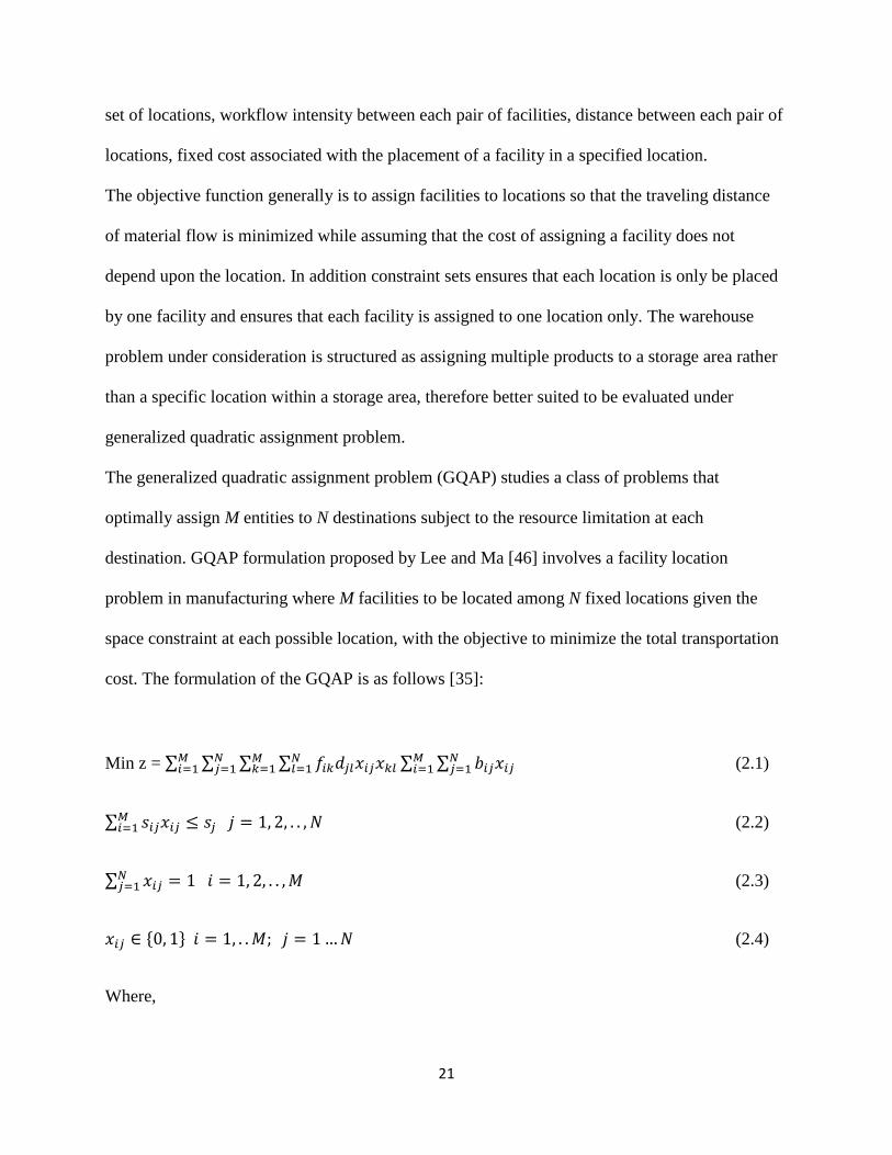
The generalized quadratic assignment problem (GQAP) studies a class of problems that
optimally assign M entities to N destinations subject to the resource limitation at each
destination. GQAP formulation proposed by Lee and Ma [46] involves a facility location
problem in manufacturing where M facilities to be located among N fixed locations given the
space constraint at each possible location, with the objective to minimize the total transportation
cost. The formulation of the GQAP is as follows [35]:
Min z = ∑ ∑ ∑ ∑
∑ ∑
(2.1)
∑ (2.2)
∑ (2.3)
{ } (2.4)
Where,

22
M the number of facilities
N the number of locations
the commodity flow from facility i to facility k
the distance from location j to location l
the cost of installing facility i at location j
the space requirement if facility i is installed at location j
the space available at location j
binary variable, with x ij = 1 iff facility i is installed at location j
The GQAP formulation was restructured to address the warehouse problem considered in this
research, where the objective function was restated to minimize the travel distance among the
storage areas to replenish and dispatch product. The GQAP formulation was evaluated for
appropriateness in addressing the warehouse problem considered in this research. It was
concluded that due to the limitations in the level of detail provided by the data from the
warehouse, the GOAP formulation is not the best suited method. Methods such as reinforcement
learning are more appropriate as they can be formulated to solve the warehouse problem even
with data limitations.

23
Chapter 3
3.1 Reinforcement Learning
In this thesis we explore RL algorithms to identify a good domain-specific heuristics to
determine appropriate location for a product type, thus reducing the time involved in
replenishing products and dispatching of inventory. An RL method recommends what to do in
order to maximize a numerical reward signal. Unlike in other machine learning methods, the
learner is not told which actions to take, but the learner discovers which actions yield the most
reward through exploration of state space. The actions may affect not only the immediate reward
but also that of the subsequent states. The trial and error search, and the delayed reward are two
most distinctive features of RL, it is different from other machine learning methods used in
research for statistical pattern recognition, and artificial neural networks which employ
supervised learning. Supervised learning extracts information and knowledge from examples
provided by a knowledgeable external supervisor. This is an important kind of learning, but
alone it is not adequate for learning from interaction [5].
The major components of RL, as discussed by Sutton and Barto [5], are highlighted in the
following paragraphs: a policy defines the learning agent’s way of behaving at a given time. It
can be thought of as a mapping from perceived states of the environment to actions to be taken
when in those states. Policy forms the core of RL, in that it alone would suffice in determining an
agent’s behavior.
A reward function defines the goal in a reinforcement learning problem. It maps the state action
pair of the environment to a single number, a reward, indicating the desirability of that state. The
objective of an RL agent is to maximize the total reward it receives in the long run.
24
The reward function is an immediate indicator in selecting the “right” state-action pair; a value
function is applied to guide the selection of the “right” actions in the long run. The value of a
state is the total amount of reward an agent can expect to accumulate over the future, starting
from the state. As rewards determine the immediate, desirability of environmental states, values
determine the long-term desirability of states after taking into account the states that are likely to
follow, and the rewards available in those states. RL agent seeks actions that bring states with
high values, not high reward, because these actions yield the highest cumulative reward in the
long run.
Sutton and Barto [5], Bertsekas and Tsitsiklis [47], and Gosavi [48] have done prominent work
in RL domain and thoroughly describe reinforcement learning method and its applications. RL
methods learn a policy for selecting actions in a problem space, the policy dictates for each state
which action is to be performed in that state. After an action is chosen and applied in state ,
the problem space shifts to state and learning system receives reinforcement ( [49].
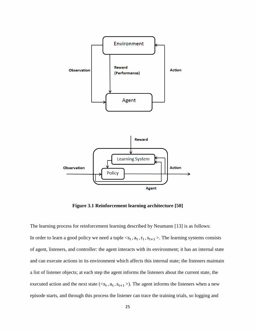
The reinforcement learning architecture is depicted in Figure 3.1. In this architecture [50], an
agent continually observes and acts in an environment, and its actions can trigger rewards to be
issued. The agent contains a policy, which determines how it responds to its observations. A
policy is characterized by a number of parameters, which form a parameter space. The agent also
contains a learning system, which uses the reward signal, or performance measure, to update the
policy via a feedback mechanism.
25
Figure 3.1 Reinforcement learning architecture [50]
The learning process for reinforcement learning described by Neumann [13] is as follows:
In order to learn a good policy we need a tuple < >. The learning systems consists
of agent, listeners, and controller: the agent interacts with its environment; it has an internal state
and can execute actions in its environment which affects this internal state; the listeners maintain
a list of listener objects; at each step the agent informs the listeners about the current state, the
executed action and the next state (< >). The agent informs the listeners when a new
episode starts, and through this process the listener can trace the training trials, so logging and

26
learning are performed simultaneously. The controller, informs the agent to execute in the
current state. This controller could calculate the Q-function; however another representation of
the policy is used by some algorithms. This process is described in the Figure 3.2 below.
Figure 3.2 The structure of the learning system, with the agent, the environment, the agent
listeners as interface for the learning algorithms and agent controllers [13]
RL approaches have been applied to solve several warehouse management problems. Zhang and
Dietterich [3] present an RL technique for a resource allocation problem, to solve a static
scheduling problem. Aydin and Oztemel [51] present a modified version of Q-learning method to
learn dispatching ruled for production scheduling. Wang and Usher [52] present Q-learning
algorithm for use by job agents when making routing decisions in a job shop environment.
Mahadevan and Theocharous [9] present an artificial intelligence approach to optimization based
on a simulation-based dynamic programming method, reinforcement learning. Reidmiller and
Riedmiller [53] present a neural network based agent to autonomously optimize local dispatching

27
policy with respect to global optimization goal, defined for the overall plant. Sui et al. [54]
propose a methodology based on reinforcement learning rooted in Bellman equation, to
determine a replenishment policy in a Vendor-Managed Inventory (VMI) system with
consignment inventory.
3.2 Application to our problem
As discussed in earlier sections of the thesis, we apply a model-free learning as opposed to
model-based learning. In model-based learning the model is learned empirically, and MDP is
solved as if the learned model is correct. Whereas, applying a model-free learning, the value
function is updated each time there is a transition, and frequent outcomes contribute to more
updates over time.
The following paragraphs will discuss the applicability of RL to the warehouse problem. As we
know it the warehouse is divided into zones and there are fourteen zones. Also known are the
distances among zones and the capacities of the zones. We assume that high arrival items are
also high shipment items. The input to the algorithm is the product type and its quantity. The
objective is for the algorithm to learn that the high frequency items are high in demand, they
move quickly so they should be placed closest to the receiving /shipping doors. The objective of
the algorithm is to minimize the transit time for product placement and dispatch, described in
equation 3.1, and it is a value that is calculated by multiplying the frequency, and distance for
each item and zone pair. So for each item number, the minimum distance from current location
of the item to a zone will be chosen based on frequency (demand in quantity of the item) of the
item. A product will be placed in a zone with the capacity to support the product quantity. Based
on the constraints of the algorithm, the product will only be placed in a zone if the required
capacity for the product quantity is available in the zone.

28
∑ ∑
(3.1)
∑ (3.2)
where,
z = the total cost for transit between waiting area by the receiving door to appropriate zone and
the location of zone item located in the exit doors
the frequency or volume of item
;
the location of the zone housing item
the capacity of zone
the required capacity for item in zone
State determination Criteria
A policy table is used so an agent can make decisions based on its current state. For this product
allocation problem, the policy table for a product maps the product's current state to zones that
the product can be placed in for the next operation. To determine the current state, the RL agent
considers product information that it is in its current knowledge, or product information that is
available on the zone under consideration. State determination criteria are based on the frequency
of a product, and distance to zone.
29
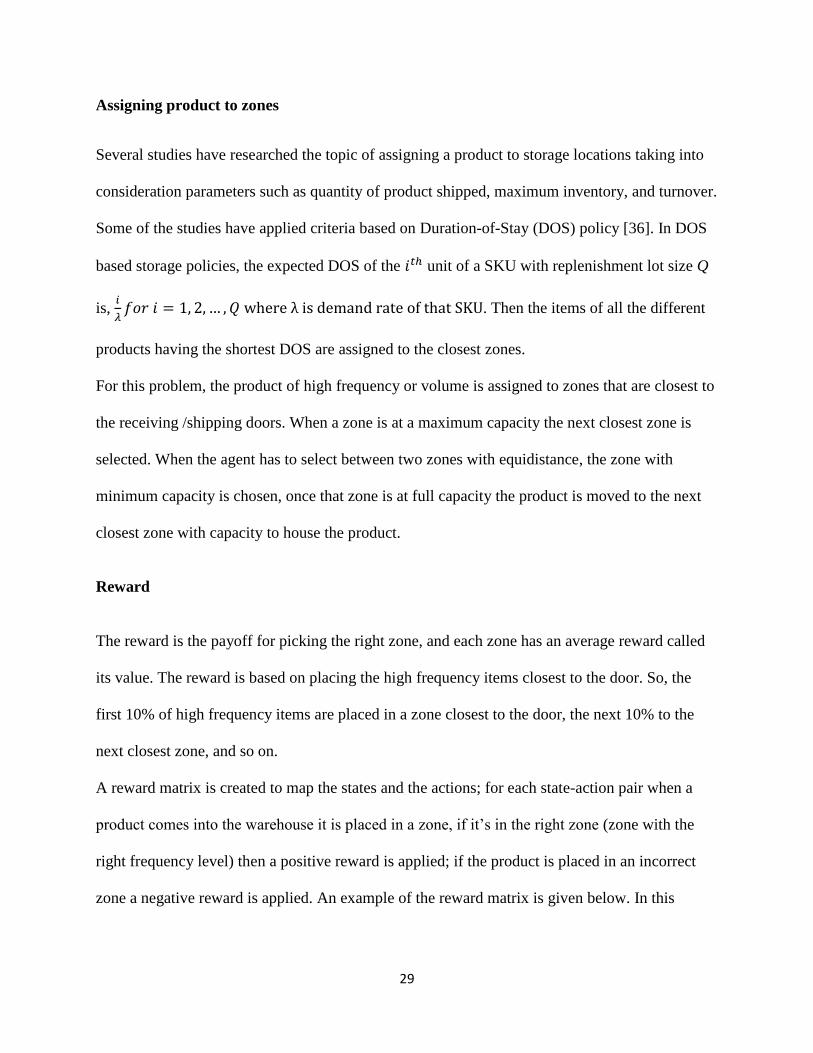
Assigning product to zones
Several studies have researched the topic of assigning a product to storage locations taking into
consideration parameters such as quantity of product shipped, maximum inventory, and turnover.
Some of the studies have applied criteria based on Duration-of-Stay (DOS) policy [36]. In DOS
based storage policies, the expected DOS of the unit of a SKU with replenishment lot size Q
is,
. Then the items of all the different
products having the shortest DOS are assigned to the closest zones.
For this problem, the product of high frequency or volume is assigned to zones that are closest to
the receiving /shipping doors. When a zone is at a maximum capacity the next closest zone is
selected. When the agent has to select between two zones with equidistance, the zone with
minimum capacity is chosen, once that zone is at full capacity the product is moved to the next
closest zone with capacity to house the product.
Reward
The reward is the payoff for picking the right zone, and each zone has an average reward called
its value. The reward is based on placing the high frequency items closest to the door. So, the
first 10% of high frequency items are placed in a zone closest to the door, the next 10% to the
next closest zone, and so on.
A reward matrix is created to map the states and the actions; for each state-action pair when a
product comes into the warehouse it is placed in a zone, if it’s in the right zone (zone with the
right frequency level) then a positive reward is applied; if the product is placed in an incorrect
zone a negative reward is applied. An example of the reward matrix is given below. In this

30
matrix the rows represent states, and the columns represent actions. For this example, a reward of
hundred was given for the correct state-action pair, and zero otherwise.
Figure 3.3 Reward matrix example
In the case that the appropriate zone is occupied to full, then the product is placed in the next
closest zone, or agent checks for special instructions such as placing the product in storage, and it
receives a positive reward. In the case that there is a conflict to place a product in a zone, then
the product with the higher frequency is given priority with a positive reward, and the other
(conflicting) product is placed in the next best zone. If the frequencies of the products are the
same, then product is chosen at random.
Policy
Policy dictates the decision making function of the RL agent. It specifies the action that should
be taken in any of the situations encountered. For this problem, we examine obtaining an
optimal policy in a model-free learning method (where model does not consist of knowledge of
the state transition probability, and the reinforcement function). This is where the agent interacts
with its environment directly to obtain information which, by means of an appropriate algorithm,

31
can be processed to produce an optimal policy [4]. Since learning Q* does not depend on
optimality of the policy used, the focus could be on exploration during learning. However, since
the learning will take place while the system is in operation, a close to optimal policy can be
applied while using standard exploration techniques ( -greedy, softmax, etc.) [55].
When the learning stops, a greedy policy is applied [55]:
( ( (3.3)
Kaelbing et al. [4] explain that as the Q values nearly converge to their optimal values, it is
appropriate for the agent to act greedily, taking in each situation, the action with the highest Q
value. During learning there is a exploration versus exploitation trade-off that is made, however,
there is no good, formally justified approach for the problem; the best approach is to apply ad
hoc strategies such as greedy strategies, randomized strategies or interval-based techniques.
Value Function
As in most reinforcement learning work, the algorithm attempts to learn the value function of
the optimal policy . Value function specifies what is good in the long run; the value of a state
is the total amount of reward the agent can expect to accumulate over the future when starting
from the current state. Rewards determine immediate desirability while value indicates the long
term desirability.
The reinforcement learning component learns a new policy that maximizes the new value
function. Value of a policy is learned through Q-learning method. The Q-learning algorithm,
introduced by Watkins in 1989 [15], is rooted in dynamic programming, and is a special case of
temporal difference ( ( when λ = 0.

32
Q-learning Methodology
Q-learning solves the problem of learning by learning a value function denoted by
. The function Q maps states and actions to scalar values. After learning, (
ranks actions according to their goodness, where larger the expected cumulative pay-off for
picking action at state , the larger the value ( [56].
The goal of Q-learning for this problem is to learn the product-zone association. At the end of a
learning iteration, the agent’s objective function values are computed and the cost function is
adjusted using Q-learning formula [57]. A matrix similar to reward matrix, is created for Q-
values. This Q-matrix represents the "knowledge" of what the RL agent has learned through the
many experiences. The rows of the Q-matrix represent current state of the agent; the columns of
Q-matrix represent the action that will transition to the next state. Initially, the agent is assumed
to no knowledge and therefore Q-matrix is a zero matrix; ( are set to zero. Let's consider
the instance where during learning the learner executes action at state , which leads to a new
state and the immediate pay-off . Q-learning uses Equation 3.4, state transition to update
( [56].
As it has been discussed before, model free learning facilitates learning through episodes or
epochs, and the estimates are updated at each transition. Over time the updates mimic Bellman
updates:
Q-value iteration (model-based, requires known MDP)
( ∑ ( ( ( (3.4)
Q-learning (model-free, requires only experienced transitions)
( ( ( ( ( (3.5)
33
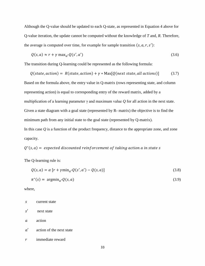
Although the Q-value should be updated to each Q-state, as represented in Equation 4 above for
Q-value iteration, the update cannot be computed without the knowledge of T and, R. Therefore,
the average is computed over time, for example for sample transition ( :
( ( (3.6)
The transition during Q-learning could be represented as the following formula:
( ( ( (3.7)
Based on the formula above, the entry value in Q-matrix (rows representing state, and column
representing action) is equal to corresponding entry of the reward matrix, added by a
multiplication of a learning parameter γ and maximum value Q for all action in the next state.
Given a state diagram with a goal state (represented by R- matrix) the objective is to find the
minimum path from any initial state to the goal state (represented by Q-matrix).
In this case Q is a function of the product frequency, distance to the appropriate zone, and zone
capacity.
(
The Q-learning rule is:
( ( ( (3.8)
( ( (3.9)
where,
current state
next state
action
action of the next state
immediate reward

34
learning rate
- discount factor and has range of 0 to 1 (0≤ γ < 1). If is closer to 0 the agent will only
consider immediate reward, and if closer to 1 the agent will consider future reward with greater
weight, willing to delay the reward. is an experience tuple.
The Q-learning algorithm adapted from [58] [59]:
Set parameter γ and the environment reward matrix R
For each , , initialize table entry ( 0
For each epoch:
Select random initial state
Do while, not reach goal state:
Select an action among all possible actions for current stat
Receive immediate reward
Using this possible action consider to go to the next state
Update the table entry for ( as follows:
( ( ( (
Set the next state as the current state ≤
End Do
End For
Input: Q-matrix, initial state
1. Set current state = initial state
2. From current state, find action that produced maximum Q value
3. Set current state = next state
35
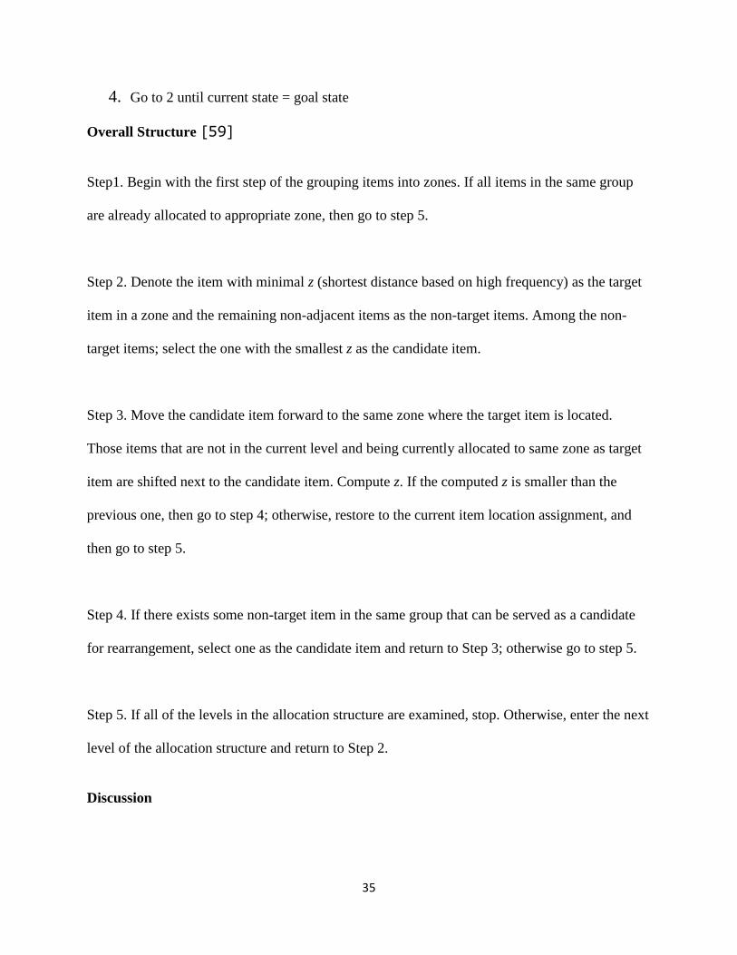
4. Go to 2 until current state = goal state
Overall Structure [59]
Step1. Begin with the first step of the grouping items into zones. If all items in the same group
are already allocated to appropriate zone, then go to step 5.
Step 2. Denote the item with minimal z (shortest distance based on high frequency) as the target
item in a zone and the remaining non-adjacent items as the non-target items. Among the non-
target items; select the one with the smallest z as the candidate item.
Step 3. Move the candidate item forward to the same zone where the target item is located.
Those items that are not in the current level and being currently allocated to same zone as target
item are shifted next to the candidate item. Compute z. If the computed z is smaller than the
previous one, then go to step 4; otherwise, restore to the current item location assignment, and
then go to step 5.
Step 4. If there exists some non-target item in the same group that can be served as a candidate
for rearrangement, select one as the candidate item and return to Step 3; otherwise go to step 5.
Step 5. If all of the levels in the allocation structure are examined, stop. Otherwise, enter the next
level of the allocation structure and return to Step 2.
Discussion

36
Based on the above algorithm the learned action-value function, , directly approximates * the
optimal action-value function, independent of the policy being followed. The policy still has an
effect in that it determines which state-action pairs are visited and updated [5].
To find the optimal function eventually, agent must try out each action in every state many
times. Watkins [15] , and Watkins and Dayan [57] show that all state-action pairs in any order
in which each state-action pair's Q-value is updated infinitely often, then the estimated * will
converge to * with probability of 1 as long as is decreased to zero gradually or at an
appropriate rate [60].
Q-learning reinforcement learning algorithm has been compared to many other models such as Q
( [60], actor-critic learning [61] classifier systems (CS) [62] and, adaptive heuristic critic
(AHC) learning. Most studies reached the same conclusion as the study conducted by Lin [63]
comparing AHC to Q-learning. The results suggested reinforcement learning to be promising
approach to build autonomous learning systems. In some cases such as studies performed by Lin
[63] Sutton [64] found superiority of Q-learning over AHC learning [65]. There are also studies
[66] which have developed algorithms similar to Q-learning, modifying the learning algorithm to
suit their application needs. Q-learning algorithm, as proved by research that has applied it to
solve warehouse challenges, is an apt methodology for the warehouse problem considered in this
thesis.
In order to achieve optimal or close to optimal conditions, monitoring and adjusting the
following critical parameters will assure the agent learns the shortest path to the highest reward:
number of iterations, the exploration rate, the learning rate, discount factors, and penalties, and
rewards.

37
Chapter 4
4.1 Concluding Remarks
There exists plethora of research and solution approaches to solve problems in the warehouse
management domain. Due to the unique challenges presented by a facility such as constantly
changing environment, facility specific variables, a solution that works for a particular problem
might prove to be ineffective for another. The research work presented in this paper focuses on
challenges faced by a local warehouse, suffering from inefficient operations from housing large
product inventory, and with additional considerations to expand the warehouse. The data
provided by the warehouse was analyzed to identify any trends and relationships between
variables such as product quantity shipped and the customer/vendor for a product type. A few
approaches such as QAP and RL were examined to effectively approach the problem faced by
the local distributor. We focused on a RL based approach. Research on RL approaches was
conducted, and a framework is presented for effective operation minimizing the distance for
product replenishment and dispatch at a local warehouse. Future work includes testing the
framework, and comparing it against optimal conditions.
38
References
1. Liu, M. Optimal Storage Layout and Order Picking for Warehousing. International Journal of
Operations Research, Vol. 1, pp. 37-46, 2004.
2. Tarkesh, H., Atighehchian, A., and Nookabadi, S. A. Facility Layout Design Using Virtual Multi-
Agent System. Asia Pacific Industrial Engineering and Management System Conference, 2004.
3. Zhang, W., and Dietterich, G. T. A Reinforcement Learning Approach to Job-Shop Scheduling. In the
Proceedings of the International Joint Conference on Artificial Intelligence, 1995.
4. Kaelbling, L. P., Littman, M. L., and Moore, A. W. Reinforcement Learning: A Survey. Artificial
Intelligence Research Vol. 4, pp. 237-285, 1996.
5. Sutton, R. S., and Barto, A. Reinforcement Learnning: An Introduction, 1st. Cambridge, MA: MIT
Press, 1998.
6. Singh, S., Barto, A. G., and Chentanez, N. Intrinsically motivated reinforcement learning. Advances
in Neural Information Processing Systems 17 (NIPS). Cambridge, MA: MIT Press, 2005.
7. Laird, J. E. The Soar CognitiveArchitecture. Cambridge: MIT Press, 2012.
8. Mahadevan, S., et al. Self-Improving Factory Simulation using Continuous-time Average-Reward
Reinforcement Learning. In Proceedings of the 4th International Machine Learning Conference, pp. 202-
210, 1997
9. Mahadevan, S., and Theocharous, G. Optimizing Production Manufacturing using Reinforcement
Learning. In proceedings of Eleventh International FLAIRS Conference, 1998.
10. Paternina-Arboleda, C. D., and Das, T. K. Intelligent Dynamic Control Policies for Serial
Production Lines. IIE Transactions, Vol. 33, pp. 65-77, 2001.
11. Crites, R., and Barto, A. Elevator Group Control Using Multiple Reinforcement Learning Agents.
Machine Learning, Vol. 22, pp. 234-262, 1998.
12. Singh, S., and Bertsekas, D. P. Reinforcement Learning for Dynamic Channel Allocation in Cellular
Telephone Systems. Advances in Neural Information Processing Systems, Vol. 9, 1997, pp. 974-980.
13. Neuman, G. The Reinforcement Learning Toolbox, Reinforcement Learning for Optimal Control
Tasks. Ph.D. thesis, University of Technology, 2005.
14. Bellman, R. Dynamic Programming. Princeton University Press, 1957.
15. Watkins, C. J. Learning from Delayed Rewards. Kings College, Cambridge, England : unpublished
Ph.D. thesis, 1989.

39
16. Hamed, T., Arezoo, A., and Nookabadi, A. S. Facility Layout Design Using Virtual Multi-Agent
System. In proceedings of the Fifth Asia Pacific Industrial Engineering and Management Systems
Conference, 2004.
17. Wang, Y. C., and Usher, J. M. Application of Reinforcement Learning for Agent-Based Production
Scheduling. Artificial Intelligence, Vol. 18, pp. 73-82, 2005.
18. Rouwenhorst, B., et al. Warehouse design and control: Framework and literature review. European
Jornal of Operational Research, Vol. 2000, pp.122, 1999.
19. Gu, J.X., Goetschalckx, M., and McGinnis, L.F. Research on Warehouse Operation: A
Comprehensive Review. European Journal of Operational Research, Vol. 177, 2007.
20. Van denBerg, J.P. A Literature Survey on Planning and Control of Warehousing Systems. IIE
Transactions, Vol. 21, 1999.
21. Cormier, G., and Gunn, E. A Review of Warehouse Models. European Jorunal of Operational
Research, Vol. 58, 1992.
22. De Koster, M.B.M., Le-Duc, T., and Roodbergen, K.J. Design and Control of Warehouse Order
Picking: A Literature Review. European Journal of Operational reseach, Vol. 182, 2007.
23. Gu, J., Goetschalckx, M. and McGinnis, F.L. Research on Warehouse Design and Performance
Evaluation: A Comprehensive Review. European Journal of Operational Research, Vol. 203, 2009
24. Ratliff, H.D., and Rosenthal, A.S. Order-Picking in a Rectangular Warehouse: A Solvable Case of
the Traveling Salesman Problem. Operations Research , Vol. 31, 1983.
25. Van den Berg, J.P., et al. Forward-Reserve Allocation in a Warehouse with Unit-Load
Replenishments. European Journal of Operational Research , Vol. 111, 1998.
26. Karasawa, Y., Nakayama, H., Dohi, S. Trade-off Analysis for Optimal Design of Automated
Warehouses. International Journal of System Science, Vol. 11, 1980.
27. Lowe, T.J., Francis, R.L., and Reinhardt E.W. A Greedy Network Flow Algorithm for a
Warehouse Leasing Problem. IIE Transactions, Vol. 1, 1979.
28. White, J.A., and Francis, R.L. Normative Models for Some Warehouse Sizing Problems. IIE
Transactions, Vol. 3, 1971.
29. Bozer, Y.A., and White, J.A. Design and Performance Models for End-of-Aisle Order Picking
Systems. Managememt Science, Vol. 36, 1990.
30. De Koster, M.B.M. Performance Approximation of Pick-to-Belt Orderpicking Systems. European
Journal of Operational Research, Vol. 72, 1994.
31. Chew, E.P., and Tang, L.C. Travel Time Analysis for General Item Location Assignment in a
Rectangular Warehouse. European Journal of Operational Research, Vol. 112, 1999.

40
32. Bartholdi III, J.J., Eisenstein, D.D., and Foley, R.D. Performance of Bucket Brigades When Work
is Stochastic. Operations Research, Vol. 49, 2001.
33. Hackman, S.T., and Rosenblatt, M.J. Allocating Items to an Automated Storage and Retrieval
System. IIE Transactions, Vol. 22, 1990.
34. Davies, A.L., Gabbard, M.C., and Reinhold, E.F. Storage Method Saves Space and Labor in Open-
Package-Area Picking Operations. Industrial Engineering, pp. 68-74, 1983.
35. Francis, R.L., McGinnis, L.F, and White, J.A. Facility layout and location: An analytical
approach, Second Edition. New Jersey: Prentice Hall, 1992.
36. Goetschalckx, M., and Ratliff, H. D. Shared Storage Policies Based on the Duration Stay of Unit
Loads. Management Science, Vol. 36, 1990.
37. Ashayeri, J., and Gelders, L.F. Warehouse Design Optimization. European Journal of Operational
Research, Vol.21, pp.285-294, 1985.
38. Chiun-Ming, Liu. Storage Layout And Order Picking For Warehousing. International Journal of
Operations Research, Vol. 1, 2001.
39. Cormier, G., and Gunn, E. A. On Coordinating Warehouse Sizing, Leasing and Inventory Policy.
IIE transactions, Vol. 29, 1996.
40. Rosenblatt, M.J., and Roll, Y. Warehouse Capacity in a Stochastic Environment. International
Journal of Production Research, Vol. 26, 1988.
41. Heragu, S.S., Huang, C.S., Mantel, R.M., and Schuur, P.M. A Mathematical Model for Warehouse
Design and Product Allocation. Troy, NY : Rensselaer Polytechnic Institute, 2003. Technical Report 38-
03-502.
42. Frazelle, E.H., et al. The Forward-Reserve Problem. [book auth.] Ciriani, T.A., and Leachman, R.C.
Optimization iin Industry.Wiley, 1994.
43. Hackman, S.T., and Platzman, L.K. Near-Optimal Solution of Generalized Resource Allocation
Problems with Large Capacities. Operations Research, Vol. 35, 1990.
44. Ji, P., and Ho, W. The Traveling Salesman and the Quadratic Assignment Problems: Integration,
Modeling and Genetic Algorithm, in Proceedings of International Symposium on OR and Its
Applications, 2005.
45. Koopmans, T. C., and Beckmann, M. J. Assignment Problems and the Location of Economic
Activities. Econometrica, 1957.
46. Chi-Guhn, L., and Zhong, M. The Generalized Quadratic Assignment. Ontario, Canada : University
of Toronto, 2004.
47. Bertsekas, Dimitri P., and Tsitsiklis, John. Neuro-Dynamiic Programming. Athena Scientific,
1996.

41
48. Gosavi, Abhijit. Simulation-Based Optimization: Parametric Optimization Techniques and
Reinforcement Learning. Boston: Kluwer, 2003.
49. Sutton, S. Richard, and Barto, G. Andrew. Reinforcement Learning: An Introduction. Cambridge:
MIT Press, 2005.
50. Nigel, Tao Chi-Yen. Walking the Path: An Appliction of Policy-Gradient Reinforcement Learning to
Network Routing. Australian National University, 2001.
51. Aydin, M. E. and Öztemel, E. Dynamic Job-Shop Scheduling Using Reinforcement Learning Agents.
Robotics and Autonomous Systems, Vol. 33, 2000.
52. Wang, Y. C., and Usher, J. M. A Reinforcement Learning Approach for Developing Routing
Policies in Multi-Agent Production Scheduling. The International Journal of Advanced Manufacturing
Technology, Vol. 33, 2007.
53. Riedmiller, S. C., and Riedmiller, M. A. A Neural Reinforcement Learning Approach to Learn
Local Dispatching Policies in Production Scheduling. In Proceedings of the Sixteenth International Joint
Conference on Artificial Intelligence, pp. 764–769, 1999.
54. Zheng, S., Gosavi, A., and Lin, L. A reinforcement Learning Approach for Inventory Replenishment
in Vendor-Managed Inventory systems with Consignment Inventory. Engineering Management Journal
Vol. 22, 2010.
55. Shimkin, N. Learning in Complex Systems. [Online].
http://webee.technion.ac.il/people/shimkin/LCS10/ch4_RL1.pdf. 2009
56. Sebastian, T., and Schwartz, A. Finding Structure in Reinforcement Learning. Advances in Neural
Information Processing Systems, 1995.
57. Watkins, C.J. C. H., and Dayan, P. Q-learning. Machine Learning, Vol. 8, pp. 279-292, 1992.
58. Teknomo, K. Kardi Teknomo's Page. http://people.revoledu.com. [Online .
http://people.revoledu.com/kardi/tutorial/ReinforcementLearning/Q-Learning-Algorithm.htm. 2006.
59. Chen, X. Introduction to Reinforcement Learning. [Online] University of Hawaii,
http://www2.hawaii.edu/~chenx/ics699rl/grid/rl.html. September 2006
60. Peng, J., and Williams, R. Incremental Multi-Step Q-Learning. Machine Learning, Vol.22, 1996.
61. Barto, A. G., Sutton, R.S., and Anderson, C.W. Nueronlike Elements that can Slove Difficult
Learning Control Problems. IEEE Transactions on Systems, Man and Cybernetics, Vol. 13, pp. 835-
846,1983.
62. Dorigo, M., and Bersini, H. A Comparison of Q-Learning and Classifier Systems. In Proceedings
from Third International Conference on Simulation of Adaptive Behavior, Vol. SAB94, 1994.
63. Lin, Long-Ji. Self-Improvement Based on Reinforcement Learning, Planning and Teaching. In
Proceedings of Eighth International Workshop on Machine Learning, pp. 323-327, 1991.
42
64. Sutton, R.S. Integrated Architectures for Learning, Planning, and Reacting Based on Approximating
Dynamic Programming. In Proceedings of the Seventh International Workshop on Machine Learning, pp.
358-362, 1990.
65. Lin, Long-ji. Self-Improving Reactive Agents Based On Reinforcement Learning, Planning and
Teaching. Machine Learning, Vol. 8, pp. 293-321, 1992.
66. Gambardella, L. M., and Dorigo, M. Ant-Q: A Reinforcement Learning Approach to the Traveling
Salesman Problem. In Proceedings of ML-95, Twelfth Intern. Conf. on Machine Learning, pp. 252-260,
1995.
67. Tompkins, J.a., et al. Facilities Planning. NJ : John Wiley & Sons, 2003.
68. Liu, C. M.Optimal Storage Layout and Order Picking for Warehousing. IJOR, Vol. 1, pp. 37-46,
2004.
69. Ji, P., and Ho, W. The Traveling Salesman and the Quadratic Assignment Problems: Integration,
Modeling and Genetic Algorithm. In Proceedings of the Fifth International Symposium on OR and it's
Applications, 2005.
70. Tompkins, A. J. The Warehouse Management Hanbook. Raleigh: Tompkins Press, 1998.
71. Roodbergen, J. K., Sharp, P.G., and Vis, I. F. A. Designing the Layout Structure of Manual Order
Picking Areas in Warehouses. IIE Transactions, 2008.
72. Chiang, W.C., Kouvelis, P., and Urban, T. Incorporating Workflow Interface in Facility Layout
Design: The Quartic Assignment Problem. Management Science, pp. 584-590, 2002.
73. Hackman, S.T., and Rosenblatt, M.J. Allocating items to an automated storage and retrieval
system. IIE Transactions, pp. 7-14, 1990.
74. Van den Berg, J.P., et al. Forward Reserve Allocation in a Warehouse with Unit-Load
Replenishments. European Journal of Operations Research, pp. 98-113, 1998.
75. Hackman, S.T., and Bartholdi, J.J. Allocating Space in a Forward Pick Area of a Distribution
Center for Small Parts. IIE Transactions, pp. 1046-1053, 2008.
76. Roodbergen, J. K., and Vis, I. F. A. A Model for Warehouse Layout. IIE Transactions, pp. 799-811,
2006.
77. Tsai, Y.C., Liou, H.J., and Huang, M. T. Using a Multiple-GA Method to Solve the Batch Picking
Problem: Considering Travel Distance and Order Due Time. International Journal of Production
Reseach, pp. 6533-6555, 2008.
78. Malmborg, C., and Krishnakumar, B. Optimal storage Assignment Policies for Multiaddress
Warehousing Systems. IEEE Transactions on Systems, Man and Cybernetics, Vol. 19, 1989.

43
79. Haijun, Z., Puxiu, Y., and Zhu, J. A Realization of Optimal Order-Picking for Irregular Multi-
Layered Warehouse. In Proceedings for International Seminar on Business and Information Management,
2008.
80. Francis, R.L., McGinnis, L.F., and White, J.A. Facility layout and location: An analytical
approach, Second Edition. New Jersey: Prentice-Hall Inc., 1974.
81. Kulturel, S., et al. Experimental Investigation of Shared Storage Assignment Policies in Automated
Storage/Retrieval Systems. IIE Transactions, Vol. 8, pp. 739-749, 1999.
44
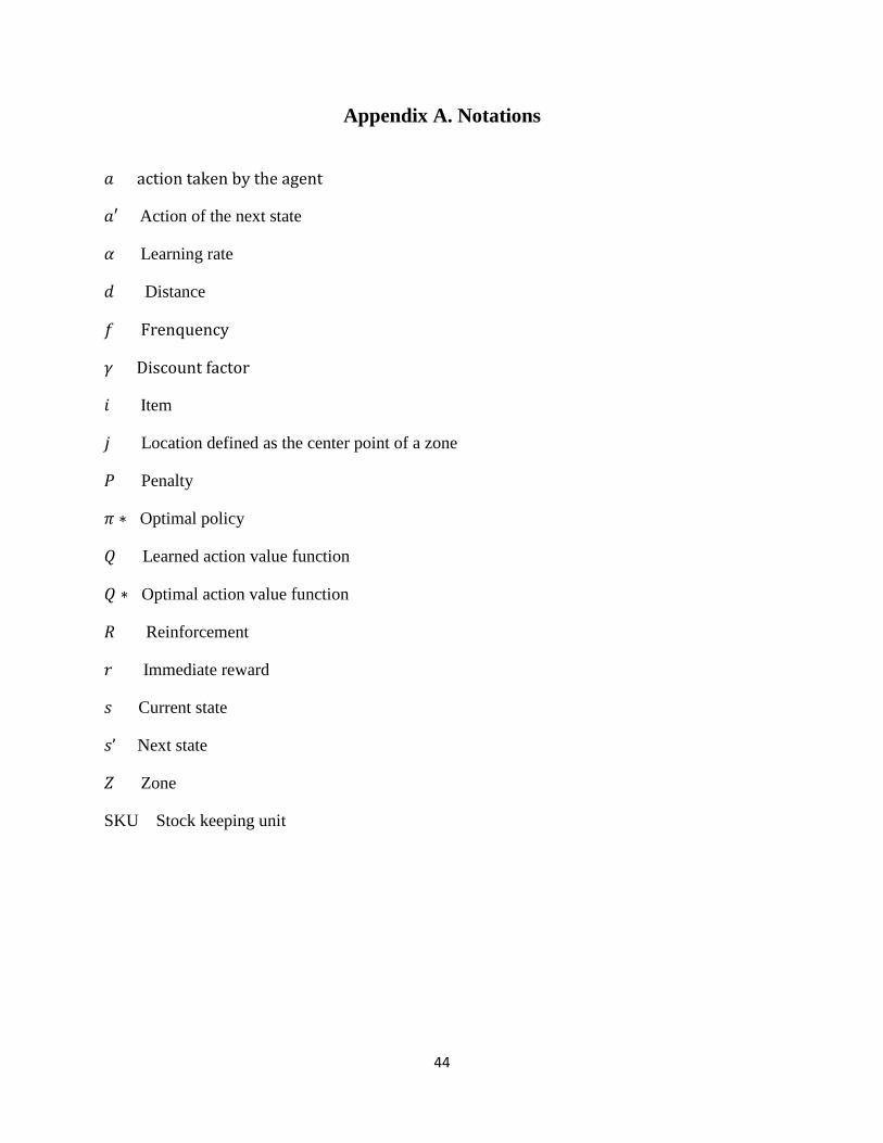
Appendix A. Notations
Action of the next state
Learning rate
Distance
Item
Location defined as the center point of a zone
Penalty
Optimal policy
Learned action value function
Optimal action value function
Reinforcement
Immediate reward
Current state
Next state
Zone
SKU Stock keeping unit

45
Appendix A. Analysis
1. Variability Analysis
Quantity shipped per item number in 2007 was pulled from the database provided the warehouse.
In the one year time period, transactions for 7,167 item numbers exist. On average 34
transactions per item number were placed during the year. Quantity shipped was as minimal as 0
and maximum of 802,070. In the SQL database, table order detail history was used to generate
data for each item number for which quantity was shipped. The following SQL query was used:
Select insert_date, item_number, qty_shipped
from t_order_detail_history
where year(insert_time) = '2007'
group by item_number
This query generates 103, 487 rows of data, with headers: Date, Item Number, and Quantity
Shipped. Below is the table for the item number 704207.
Date Item Number Quantity Shipped
1/6/2007 704207 17710
1/13/2007 704207 4014
1/20/2007 704207 6164
1/27/2007 704207 2124
2/3/2007 704207 5456
2/10/2007 704207 4444
2/17/2007 704207 4612
3/31/2007 704207 43586

46
4/21/2007 704207 26998
4/28/2007 704207 5898
:
.
:
.
:
.
Quantity Shipped over time for Item Number 704207
The query is used in a program coded in C# to study the shipping distribution of the product.
Steps involved are as follows:
Step 1: Generate rows for days for which there were no transactions
Date Item Number Quantity Shipped
1/1/2007 704207 0
1/2/2007 0
1/3/2007 0
1/4/2007 0
1/5/2007 0
1/6/2007 17710
1/7/2007 0
1/8/2007 0
1/9/2007 0
1/10/2007 0
1/11/2007 0
1/12/2007 0
1/13/2007
:
.
4014
:
.
For each item number
Step 2: Calculate the mean, and standard deviation, for quantity shipped
= 15463.99
Where,

47
And = √∑
Step 3: Calculate:
Date Item Number Quantity Shipped
1/1/2007 704207 0 -0.113472982
1/2/2007 0 -0.113472982
1/3/2007 0 -0.113472982
1/4/2007 0 -0.113472982
1/5/2007 0 -0.113472982
1/6/2007 17710 1.031768225
1/7/2007 0 -0.113472982
1/8/2007 0 -0.113472982
1/9/2007 0 -0.113472982
1/10/2007 0 -0.113472982
1/11/2007 0 -0.113472982
1/12/2007 0 -0.113472982
1/13/2007 4014 0.14609778
1/14/2007
:
.
0
:
.
-0.113472982
:
.
Step 4: Measure variability by calculating: √∑ (
= 1.4233
Date Item
Number
Quantity
Shipped (
1/1/2007 704207 0 -0.113472982 0
1/2/2007
0 -0.113472982 0
1/3/2007
0 -0.113472982 0
1/4/2007
0 -0.113472982 0
1/5/2007
0 -0.113472982 1.311577423
1/6/2007
17710 1.031768225 1.311577423
1/7/2007
0 -0.113472982 0
1/8/2007
0 -0.113472982 0
1/9/2007
0 -0.113472982 0
1/10/2007
0 -0.113472982 0
1/11/2007
0 -0.113472982 0
1/12/2007
0 -0.113472982 0.067376981

48
1/13/2007
4014 0.14609778 0.067376981
1/14/2007
:
.
0
:
.
-0.113472982
:
.
0
:
.
∑ (
= 737.41
The results of this equation gives variation of the quantity of products shipped from one day to
the next. The products that ship at a lower volume than others were expected to return higher
variances. When looked closely (Graph 2) the high volume products appear to have a higher
variance, but relatively speaking it seems almost the same.
The graph below is variation factor plotted against a log scale
1.41
1.42
1.43
1.44
1.45
1.46
1.47
1.48
0 100000 200000 300000 400000 500000 600000 700000 800000 900000
Var
iati
on
Rat
io
Qty Shipped

49
2. Network Analysis
Initial analysis of the network formed a simple unweight, undirected graph that it has 4597 nodes
and 65474 edges. The network is a single connected component that consists of 458 vendors and
4139 customers.
Degree Distributions
The network has an average degree (x) of 28.5 and density of (disregarding weights) 0.0062.
Average degree of the network represents the average number of connections of an entity
(customer/ vendor). The network is converted into a directed graph which information/ supply
flows from vendor to customer. So that out-degree represents the supply from vendor and in-
degree represents the demand by customers. Figure 1 and 2 presents the cumulative distribution
for the in-degree and out-degree distributions (in-degree: the distribution of number of vendors
that a customer has deals; out-degree: the distribution of number of customers that a vendor
1.41
1.42
1.43
1.44
1.45
1.46
1.47
1.48
0 1 2 3 4 5 6 7
Var
iati
on
Rat
io
Qty Shipped

50
provide supplies), respectively. Assuming that the data are drawn from a distribution that follows
a power law, the estimates of the scaling parameters and the lower bounds on the scaling region
for the in-degree and out-degree distributions are; 00.05.3ˆ i , 68.009.2ˆ o , and
5.05.20ˆmin
ix , 1.4513.383ˆ
min o
x , respectively. However, the goodness of fit test
generates a p-value, p = 0.0 for both distributions that shows the power-law distribution is not a
plausible fit to the data.
Cumulative in-degree distribution on a log-log scale

51
Cumulative out-degree distribution on a log-log scale
Average Path Length
An average path length (l) between all pairs of entities in the network was calculated. Here, the
network is treated as an undirected network. The typical distance between a pair of entities in
terms of supply-demand links is about 2.27; this implies that any node can reach any other node
in the network in a relatively small number of steps. This characteristic phenomenon is called the
small-world effect.
Diameter
The maximum separation in pairs of entities was calculated to be approximately 6.
Clustering Coefficient

52
In the present study, clustering coefficient C for the network refers to the probability that any
two customers of a vendor have themselves a connection in terms of supply-demand link. The
clustering coefficient of the network is zero. This indicates that the network is a tree. This is an
expected result since the case of being an entity with both customer and vendor attributes is not
present in our network.

53
3. Code
The following SQL code was developed for customer, vendor, and product type analysis:
select distinct
c.customer_id , tr.vendor_code
from t_order_history o, t_customer c, t_order_detail_history odh,
(select distinct item_number,vendor_code
from t_receipt_history ) tr
where odh.order_number= o.order_number
AND odh.wh_id = o.wh_id
AND o.wh_id = c.wh_id
AND o.customer_id = c.customer_id
-- AND odh.wh_id = tr.wh_id
AND odh.item_number = tr.item_number
AND year(odh.insert_time) = '2007'
The following code was developed for variability analysis:
namespace WalkerCSharp
{
class Program
{
static void Main(string[] args)
{
string inputFile = "MS_Walker.txt";
string outputFile = "Variance.txt";
StreamReader input = new StreamReader(inputFile);
StreamWriter output = new StreamWriter(outputFile, false);
output.AutoFlush = true;
Dictionary<double, List<KeyValuePair<DateTime, double>>> storedValues = new
Dictionary<double, List<KeyValuePair<DateTime, double>>>();
//read the input file
string s = "";
while ((s = input.ReadLine()) != null)
{
string[] curLine = s.Split('\t');
DateTime currentDate = Convert.ToDateTime(curLine[0]);
double currentItemNumber = Convert.ToDouble(curLine[1]);
double currentZValue = Convert.ToDouble(curLine[2]);

54
if (storedValues.ContainsKey(currentItemNumber))
{
storedValues[currentItemNumber].Add(new KeyValuePair<DateTime,
double>(currentDate, currentZValue));
}
else
{
List<KeyValuePair<DateTime, double>> zValues = new
List<KeyValuePair<DateTime, double>>();
zValues.Add(new KeyValuePair<DateTime, double>(currentDate, currentZValue));
storedValues.Add(currentItemNumber, zValues);
}
}
int count = 0;
//Compute variance
foreach (double itemNumber in storedValues.Keys)
{
//add missing rows
List<double> adjustedItemNumberQuantities = new List<double>();
List<KeyValuePair<DateTime, double>> itemNumberQuantities =
storedValues[itemNumber];
DateTime previousDate = new DateTime(2007, 1, 1);
DateTime currentDate = new DateTime();
for (int i = 0; i < itemNumberQuantities.Count; i++)
{
currentDate = itemNumberQuantities[i].Key;
while (previousDate < currentDate)
{
adjustedItemNumberQuantities.Add(0);
previousDate = previousDate.AddDays(1);
}
adjustedItemNumberQuantities.Add(itemNumberQuantities[i].Value);
previousDate = previousDate.AddDays(1);
}
currentDate = currentDate.AddDays(1);
DateTime lastDay = new DateTime(2007, 12, 31);
while (currentDate <= lastDay)
{
adjustedItemNumberQuantities.Add(0);
currentDate = currentDate.AddDays(1);
}
double variance = Variance(adjustedItemNumberQuantities);

55
if (variance.Equals(Double.NaN))
{
variance = 0;
}
Console.WriteLine(itemNumber + " " + variance);
output.WriteLine(itemNumber + " " + variance);
count++;
}
Console.WriteLine("Number of items processed" + " " + count);
output.WriteLine("Number of items processed" + " " + count);
}
public static double Average(List<double> QtyShipped)
{
double QtyShippedSum = 0;
for (int i = 0; i < QtyShipped.Count; i++)
{
QtyShippedSum += QtyShipped[i];
}
return QtyShippedSum / QtyShipped.Count;
}
public static double StandardDeviation(List<double> QtyShipped)
{
double sumOfDerivation = 0;
double average = Average(QtyShipped);
for (int i = 0; i < QtyShipped.Count; i++)
{
sumOfDerivation += Math.Pow((QtyShipped[i] - average), 2);
}
return Math.Sqrt(sumOfDerivation/364);
}
public static List<double> CalculateZValues (List<double> QtyShipped)
{
List<double> zValues = new List<double>();
double average = Average(QtyShipped);
double stdv = StandardDeviation(QtyShipped);
for (int i = 0; i < QtyShipped.Count; i++)
{
double ziValue = (QtyShipped[i] - average);

56
zValues.Add((ziValue / stdv));
}
return zValues;
}
public static double Variance(List<double> QtyShipped)
{
double zSummation = 0;
List<double> zValues = CalculateZValues(QtyShipped);
for(int i = 1; i < (zValues.Count); i++)
{
zSummation += Math.Pow((zValues[i] - zValues[i - 1]), 2);
}
return Math.Sqrt(zSummation / 364);
}
}
}