regulatory wacc for australia post wacc for australia... · regulatory wacc for australia post...

Regulatory WACC for Australia Post Commentary June 2009 DRAFT Value Adviser Associates Pty Ltd Melbourne Adelaide Level 2 Level 2 65 Southbank Boulevard 99 Frome Street Southbank VIC 3006 Adelaide SA 5000 tel 61 3 9626 4300 tel 61 8 8111 4035 fax 61 3 9626 4301 fax 61 8 8111 4098 www.vaassociates.com.au

Table of Contents

Introduction.................................................................................................................................3 Conceptual Framework............................................................................................................3 Capital Asset Pricing Model .....................................................................................................5 Market Risk Premium..................................................................................................................7 Key Points ..........................................................................................................................................7 Estimate or MRP from Historical Data...........................................................................................8 Estimate of a forward MRP from Dividend Discount Model ..................................................10 Estimate of MRP from Current Market Data .............................................................................12 Term of the Risk Free Rate.......................................................................................................17 Interaction between Spot Rates and Average Rates in the CAPM ................................20 Impact of Imputation Tax on Australia Post .........................................................................24 Beta of Equity............................................................................................................................26 Appendix 1: Method of including Imputation Tax Yield in the Historical MRP...............28 Appendix 2: Comparable Analysis for Estimating Beta ....................................................30 Selected References ...............................................................................................................31

Introduction Australia Post has asked us to provide expert advice on matters relating to its Weighted Average Cost of Capital [“WACC”] as input to a price review by the ACCC. In this document we comment on:

• The underlying conceptual framework relating to the WACC; • The market risk premium for which we recommend 7% as the appropriate long

term forward looking rate; • The appropriate term of the risk free rate used in the CAPM and for estimating the

cost of debt which we argue should be 10 years; • Interactions between spot and average rates in CAPM supporting our

recommendation of 7% for the MRP • The value of Imputation tax credits which are zero for Australia Post given it does

not distribute them nor does the shareholder claim them against personal tax; • A beta of equity of 1.0 derived from updating the prior comparable set .

Conceptual Framework1 To attract capital to fund activities, a business must be expected to earn at least a sufficient profit or cash flow to meet a required return commensurate with the risk of the business, while preserving the base capital provided. The weighted average cost of capital is an estimate of the minimum return required to attract debt and equity capital in the proportions reflected in the WACC - it is an opportunity cost concept and should reflect the return an investor could earn on an alternative investment with similar risk and time horizon. A basic tenet of finance theory is that investors act as if they require a reward for bearing risk. The required reward is usually expressed in terms of a positive premium over a “risk free” rate of return2 for investing in assets – either ‘real’ assets or claims on real assets such as financial assets. The required total reward for capital bearing risk and for the time that capital is tied up in assets or projects can be expressed in the cost of capital of the asset or investment. The cost of capital is an input to price determination hearings in a number of regulatory price jurisdictions in Australia. These determinations consider a return on capital to be an appropriate economic cost of doing business and an estimate of it is built in to an assessment of regulatory revenue requirements.3 The overarching guide for assessing this cost of capital is that it should reflect the rate of return required in a competitive capital market that is supporting investment in real assets. Current theories suggest that this required rate of return should be independent of ownership. Regulatory bodies in Australia look to a competitive market to guide an assessment of what the appropriate cost of capital should be for assets over which they influence the pricing or outputs. The challenge for regulators is to ensure the cost of capital is set to earn investors a competitive rate of return to encourage investment but

1 Sections of this paper draw on recent our submissions to the AER, including Officer RR and SR Bishop, “Market Risk Premium: A Review”, September 2008 and Officer RR & SR Bishop’ “Market Risk Premium: Further Comments”, January 2009 2 There is no such thing as risk-free return, when the finance literature talks of a risk-free rate they mean a rate that reflects low and relatively constant risk such as the rate on government backed (in their currency) paper (debt). 3 For example the Annual Revenue Requirement(ARR) of a viable company must be equal or greater than the: operating costs + depreciation + cost of capital (the required return on capital times the value of capital) + effective tax.

not lead to monopolistic pricing while providing an incentive to improve overall performance. The cost of capital is estimated as a weighted average of the cost of debt and the cost of equity. In general this ‘plain vanilla’ weighted average cost of capital can be expressed as: WACC = kd D/V + ke E/V (1) Where ke is the expected return on equity of cost of equity kd is the expected return on debt or cost of debt

D/V is the market value of debt as a proportion of the market value of equity and debt

E/V is the market value of equity as a proportion of the market value of equity and debt which is (1 – D/V)

V is the market value of debt plus the market value of equity The ‘plain vanilla’ WACC does not have any tax effect built into it as these are assumed to be captured in the cash flows.4 The cost of debt is usually estimated as a benchmark risk free rate plus a premium for risk. The premium, it is argued, is related to liquidity, specific default and systematic risk. The cost of equity is not directly observable – its cost is less transparent than debt. It is generally estimated using the capital asset pricing model [“CAPM”]. The CAPM describes the cost of equity capital as equal to the risk free rate of return plus a premium for the risk of the equity invested. This premium is a function of market risk premium [“MRP”] times the relative risk of the equity compared with the risk of the market (beta of equity). As a consequence, the MRP is an important input to price determinations. The CAPM equation is:

efmfe ]r)k~(E[r)k~(E β−+= (2) Where E( ek~ ) is the expected return on asset e or cost of equity if the asset is equity rf is the nominal risk free rate of return E( mk~ ) is the expected return on the market portfolio

[E( mk~ ) – rf] is often called the expected market risk premium [“MRP”] being the amount by which investors will be rewarded for bearing the risk of the market portfolio which has a beta of 1

βe is the risk of asset e relative to the risk of the market or equity beta. In principle the CAPM could be used to estimate both the cost of debt and the cost of equity since both are risky assets however the cost of debt is based on a risk free rate plus a premium estimated outside the CAPM. Consequently the overall WACC can be expressed as: WACC = (rf + debt premium) D/V + efmf β]rk[r( −+ ) E/V (3) From this equation we can see that the risk free rate is generally used for two (related) purposes in establishing the cost of capital for price determinations. One is to use as a base reference rate when establishing the cost of debt, the other is an input to the CAPM

4 See Officer RR, “The Cost of Capital Under an Imputation Tax System” Accounting and Finance, May 1994

used to assess the cost of equity. In the latter case it appears as the first term in the CAPM equation and as a deduction for the expected market return to define the market risk premium (“MRP”). It is desirable that the risk free rate be the same in all ‘appearances’ in equation (3) i.e. it has the same maturity or at least essential that it is used consistently when estimating a spread and when applying that spread to a risk free rate. Capital Asset Pricing Model Under the simplest version of the Capital Asset Pricing Model5, investors choose a portfolio of assets that maximise their return for a chosen level of risk. With the existence of a risk free asset, all investors will choose some combination of the risk free asset and a market portfolio6. The mix of the risk-free asset and the market portfolio will depend upon individual attitudes to risk. With this outcome, the risk of any particular asset will be its contribution to the risk of the ‘market’ portfolio. The individual asset’s contribution to the risk of an “efficient portfolio” (the market portfolio) can be shown to be covariance7 of the assets returns with the market’s return rather than the individual variance of the asset’s returns. The total risk of an asset from an investor’s perspective is not the relevant risk – it is the sub element called systematic risk or covariance risk which is the risk that contributes to the non-diversifiable market risk. This systematic risk when divided by the variance of the market portfolio is referred to as beta. The CAPM is a forward looking concept but because of the lack of reliability in forecast models the parameters are generally estimated by reference to historical returns8. It is also common for MRP to be estimated in this way. We elaborate on this point later in the paper. Some key features of the model for the purposes of this paper are that it:

• is forward looking; • defines a positive reward for bearing risk i.e. a market risk premium will be

positive; • is a one period model of no particular time dimension; • applies to all assets which also defines the market portfolio.

The model is relatively uncomplicated however it lacks specificity if it is to be used in practice. A number of questions need to be addressed when using it, for example:

• What is the length of the ‘one period’? - Conceptually it is the price setter’s horizon but typically there is an

assumption of some match between the asset life and investor’s planning horizon. Returns are usually expressed per annum returns.

• What is the market?

5 The model generally attributed to Sharpe, Lintner, Mossin. 6 The portfolio must lie on the “efficient set”, the portfolio usually chosen is a broad based share market portfolio, each share weighted by capitalisation. 7 Covariance can be thought of as how that return on an asset changes when the market changes. Not all the changes in an assets return are due to the market. The CAPM focuses on the element of movements in returns related to market movements. 8 This is discussed further in Section 3.1 on page 5

- Conceptually it is all assets, however practically it is assumed that a broadly based equity market index is a good proxy.

• What is the expected return on the market, or the MRP, given the risk free asset?

- The emphasis should be on a forecast of the market risk premium however, in practice, it is estimated with reference to historical returns on the grounds that these influence investors’ view of the future and that there is no better forecasting model available.

- There is also a need to specify the tax status of the return on the market and the components of the return. The observable return on an equity market index is after corporate but before personal tax. The existence of an imputation tax system means that, if the benefits are valued, they should be included in the index as a component of the return. This flows from corporate tax really representing a pre-payment of personal tax for investors who can access the imputation tax rebate.

• What is beta of individual assets? How is it estimated?

- Typically the market model9, which can be thought of as consistent with an ex post (or empirical analogue) version of the CAPM, is used to estimate beta by a linear regression10 of the historical returns of a stock against the market’s returns.

- There is a particular challenge in estimating betas for unlisted businesses or business units of a multi-business unit company.

All of these questions have been subject to considerable debate and research. Arising from this research, some ‘near’ conventions have been established by academics, practitioners and regulators but there remain many areas of judgment. We summarise the areas we take as conventional and highlight the areas where we need to exercise judgment and what the trade-offs might be. Areas where convention has arisen Area “Near Convention” Long term investor horizon 10 year view for risk free rate and MRP Period of estimation of MRP Annual Method of averaging when using historical data Arithmetic average Market portfolio of risk assets Represented by a broad domestic

equity market index.

9 The market model is simply an algebraic relationship between the return on an asset and the return on the market generally expressed as ε~r~βαr~ mi ++= 10 Usually, but not necessarily, by using the statistical technique called Ordinary Least Squares regression

There are a number of areas where some element of judgment is required to form a view about an appropriate MRP to use when applying the CAPM, especially in a regulatory environment. These will be addressed later in the paper and include: Areas generally requiring judgment Area Comment Weight to place on historical versus forward looking estimates of MRP

The use of observed or historical MRP as a forward looking estimate assumes the past will repeat itself, in effect, there is ‘mean reversion’ exhibited by the estimates of the parameter. Using such a measure implies investors’ view of the future is based on experience and that there has not been any significant structural change in the forces that determine a MRP. A challenge in using a forward looking model has been that there has not been a well accepted and tested method of forecasting a variable MRP – however progress is being made in this regard which we refer to later

Accuracy Observed MRPs have a large standard deviation or variance making accuracy to multiple decimal points suggest a degree of accuracy that isn’t really there.

The value of imputation tax benefits:

It is clear that these are of value to domestic investors but not to foreign investors due to the lack of a direct market for imputation tax benefits. We do not form an explicit view about their value in this paper for estimating the MRP other than to assume they are worth more than 20 c in the dollar – to be consistent with Officer and Bishop (2008).

Market Risk Premium Key Points The required return of equity investors (or cost of equity as it will be referred to henceforth) is generally derived from the CAPM. As noted the CAPM is a forward looking model – it guides an assessment of what equity investors require to compensate them for time and risk over the period of interest. Our challenge is to estimate the forward looking, or ex ante, components viz., risk free rate, beta and MRP. We focus on the MRP in this section which is defined as the expected return on the market, E(rm), less the risk free rate. The most critical parameter is the expectations operator (E). The expectations operator should be thought of as the mean or average of the market’s forecast of future or required (expected) returns before they will invest in the equity of ‘average’ risk (beta of 1). Ideally, what we need is some method of forecasting investor’s expectations or equivalently their required returns for the different risk class of assets, averaged over all classes to capture the market view. Unfortunately, while such models exist, they require additional assumptions about investor behaviour and rarely have very much to offer in the way of forecast-ability. In an investment environment, this is perhaps not surprising insofar as if there were forecast abilities in these models then this would remove elements of risk and make the models redundant insofar as they are based on risk or stochastic returns. Our view is that the ex-ante MRP is probably not constant and cannot be adequately represented by a stable distribution. Unfortunately, however, the theory as to what might cause the parameters of the distribution (and thus the mean ex-ante MRP) to change is not well developed. This makes forecasting changes difficult, if not impossible. Moreover,

given the volatility of ex post market excess returns, even detecting such a change after the event is almost impossible. In such circumstances, it is perhaps inevitable that forecasts, in order to be objective, rely heavily on historical data. The reason for relying on such data is that the expectations of investors will be framed on the basis of their experiences, which are of course historical. Therefore the mean of historical distributions of returns or models framing returns could be expected to have had the greatest influence on investors’ expectations about the future. Hence the reliance on some average of historical MRPs in order to settle on an estimate of the investor’s expected or required MRP. Under these circumstances a longer time series is best as it will not only improve statistical ‘accuracy’ but also best weight events according to the likelihood of occurrence. For example, a short time period that incorporates the 1987 crash could potentially overweight that event compared to its likelihood of occurrence. Similarly, we note that observed market return for 2008 was a negative 40.4%, the lowest in the 127 year history of market returns available to us. This will be over-weighted in a short time horizon. An alternative approach to estimating a MRP from historical data is an explicit forward looking approach. One approach is to use a version of the constant growth dividend discount model; another emerging approach is to use information from forward markets. We now examine estimates of the MRP from both an historical and from a forward looking perspective. From a forward perspective, we examine estimates from the Dividend Discount Model, from implied volatility of market indexes and from debt markets from a forward looking perspective. Forward looking estimates currently provide a current MRP above the historical average. Estimate or MRP from Historical Data The historical risk premium over different periods has been estimated by Officer and Bishop (2009) and others for a recent review by the Australian Energy regulator (“AER”) of the weighted average cost of capital parameters for electricity transmission and distribution network service providers11. Our calculation of the historical MRP, as presented in Table 1, is assessed by examining the excess realised rate of return over a year for an investor who invests in the market portfolio and the proxy for the risk free rate at the beginning of the year. Thus the MRP is calculated as the realised market rate of return less the opening yield on a proxy for the risk free rate. The stock market return data was drawn from a number of sources:

• Research by Professor Officer as published in 198912; • Summary data published by Brailsford et al13; • ASX index and dividend data as available through Bloomberg; and • Commonwealth Government Security yield data as provided by the Reserve

Bank of Australia. It is essential to recognise that Stock market accumulation indices computed in Australia reflect a dividend yield plus a capital gain yield. They do not contain any yield from

11 Officer RR & SR Bishop, “Market Risk Premium: Further Comments” Submission to AER, January 2009; Australian Energy Regulator, “Review of the weighted average cost of capital parameters: Electricity transmission and distribution network service providers”, May 2009 12 Officer, R. R. (1989), ‘Rates of Return to Shares, Bond Yields and Inflation Rates: An Historical Perspective’, in Ray Ball, Philip Brown, Frank J. Finn and R. R. Officer(eds.), Share Markets and Portfolio Theory: Readings and Australian Evidence, University of Queensland Press 13 Brailsford T, J Handley & K Maheswaran, “Re-examination of the historical equity risk premium in Australia,” Accounting and Finance, 48, (2008) pp 73-97

imputation tax benefits that have arisen from the introduction of the imputation tax system in July 1987. One reason for the introduction of imputation tax system was to offset the otherwise double taxation of dividends. Under the prior classical tax system, dividends were taxed firstly at the corporate level since they are paid out of after corporate tax earnings and secondly at the personal level since dividends are treated as taxable income. Under the imputation system, corporate tax paid can be viewed as a prepayment of personal tax for Australian Resident Taxpaying Personal Investors (ARTPI). Since we are interested in estimating the pre- personal but post- corporate tax rate of return from the ‘market’ we would be understating the return by ignoring any value associated with imputation tax benefits that could be attributed to personal tax savings. Thus the market return for a period should contain potentially three components:

1. dividend yield; 2. capital gain yield; and 3. imputation tax yield arising from any distribution with dividends.

To include a rate of return for imputation tax benefits requires knowledge of the market value of these credits. We do not present a view on the value of these credits in this paper however we have estimated a rate of return component to include the market return based on a range of values for a dollar of imputation tax credits distributed. While we ague later that there should not be an adjustment to the cost of capital or tax component of cash flow estimates for Australia Post, it is appropriate to adjust the MRP for the imputation yield. The MRP is market wide while the tax paid by Australia Post is specific to it and not influenced by the MRP. A detailed description of our adjustment to the historical MRP to account for imputation tax benefits is provided in Appendix 1. In summary, estimates of the value of franking credits [“VFC”] for the thirteen years from 1993 to 2005 indicate an average value for the VFC of 85 basis points if the value of a dollar of franking credits distributed (φ) is 0.5. This would suggest an increase in the market rate of return for the period by an average of 0.85%. For example if the MRP for the period or the expected MRP was 6% then it should be adjusted to 6.85% for the effective value of the franking credits. This is not a large amount and well within the range of standard measurement errors one might expect from estimates of the MRP. However, on the basis of such an estimate, given a value of 0.5 for imputation tax credits distributed, in our view an MRP of 7% is more justifiable than one of 6%. Further the recent AER assessment of 0.65 further increases the merit of the increase. Added strength for this view arises from most historical averages (across different periods) being greater than 6%. Research subsequent to Officer, by Brailsford et al14, revised the market return data used by Officer prior to 1958. We do not have access to this data. Consequently we have used the summary data from Brailsford et al to estimate the summary information in Table 1 for the periods commencing 1883 whereas we used our own data sources for the period commencing 195815. The market returns, and consequently the MRP, for the original Officer series are higher for the period 1883 to 1958 as implied by the data in Table 1.16

14 Op cit 15 We broke the entire period into 1883 to 1957 and 1958 to the end year. Brailsford et al summary data was used for the former period and Officer and Bishop data used for the latter period. 16 See both Brailsford and Officer and Bishop for further comments.

Table 1: Historical Market Risk Premium

From

To

MRP with no FTC

With gamma 0.5

With gamma 0.65

Brailsford et al adjustment to Officer Data 1883 2007 6.4 6.5 6.6 1958 2007 6.7 7.1 7.2

1883 2008 5.9 6.1 6.1 1958 2008 5.7 6.0 6.1 1958* 2008 6.0 6.3 6.4

Officer Data 1883 2007 7.5 7.7 7.8 1883 2008 7.1 7.2 7.3

* Adjusted to reflect 1 in 126 year weight Table 1 shows that the long term historical MRP with gamma at 0.5 was 6.5% for the longest time period and 7.1% to 2007 and 6.5% for the period with the more reliable data (1958 to 2007).17 The addition of 2008 changes these averages to 6.1% and 6.0% respectively. Clearly the impact is greatest for the shorter time period because the large negative result for 2008 received a much greater weight than in the longer time series. We have adjusted the 1958 to 2008 series to show the impact of the unusual 2008 year i.e. one that reflects a 1 in 126 year history rather than the 1 in 51 year history in the 1958 to 2008 period. This supports the use of the longest period possible to give ‘unusual’ events the most appropriate weighting. Overall our assessment of the MRP from the historical series suggests an MRP in the range 6.1 to 7.2% when the adjustment for imputation tax credits is included. Clearly this is a long term average and applicable for a cost of capital assessed with a long term view. A challenge we have in recommending a number in this range is that we are strongly of the view that the MRP appropriate for the regulatory period is highly likely to be above this range. This comment is based on our assessment of the forward looking MRP to which we now turn. Our assessment of this information is that the market will require a return above the historical long run average in the next regulatory period for Australia Post. Estimate of a forward MRP from Dividend Discount Model The dividend discount model has been used as a method for estimating a forward looking MRP. The approach typically involves firstly deriving the implied required rate of return on equity (ke) from the current share prices of a security and market participant’s expectations of the future cash flows. The model used is a form of the dividend discount model defined with two (or sometimes three) stages of forecasts as:

17 Simply adding the value of franking credits to historical data to arrive at an implied cost of capital under an imputation tax assumes that the introduction of such a tax has no effect on the cost of capital other than the value of the imputation credits. Such an assumption is likely to be wrong in a ‘closed economy’ but reasonable in an ‘open economy’ where there are significant international movements in finance and the country’s capital market is small relative to world capital markets.

nee

1nn

1tt

e

t0

)k1)(gk(D

)k1(D

P+−

++

= +

−∑ (4)

A single stage version is:

)gk(D

Pe

t0 −

= (5)

This can be re-arranged into the cost of equity capital being equal to a dividend yield plus a growth rate, i.e.

gPD

k0

1e += (6)

The first stage in equation (4) has explicit forecasts of dividends (or equity cash flows) for n periods followed by a constant growth in perpetuity form like equation (6). The equation is re-arranged to solve for the discount rate ke. This can be undertaken for each company and weighted by market capitalisation to derive an overall market ke. The final step is to deduct an estimate of the risk free rate to derive a ‘forward’ estimate of the MRP. This simpler approach represented in equation (6) was followed by CEG in a submission to the AER in the recent WACC parameter determination while a form similar to equation (5) is followed by Bloomberg on a regular basis across a broad range of countries. The CEG approach is similar to that followed by AMP Capital, Davis18, Grey & Hall19 and Lally20. Using recent 2009 data, CEG estimate the MRP from a direct estimate of the market dividend yield and a growth rate. CEG estimate the current cost of equity for the market to be around 16 per cent. Deducting the current yield on CGS of around 4 per cent, they estimate the MRP to be around 12 per cent. CEG consider this is a long term estimate of the MRP. This is well above the findings of AMP (4.5 – 5.0%)21, Davis (4.5 – 7.0%), Grey (5.6 – 5.9%) and Lally (4 – 5.7%). This wide range of estimates reflects the different economic conditions in addition to the estimation challenges in the inputs. Clearly the CEG estimate reflects the current high risk environment collaborated by the implied increase in volatility presented below.22 Bloomberg provides its’ estimate daily but a history is not readily available from data files (from our enquiries, it appears Bloomberg does not store the information prior to July 2008). Officer and Bishop (2009) present several snapshots of its data from various sources and this is reproduced in Table 2 below. 18 K. Davis, “The weighted average cost of capital for the gas industry”, Report prepared for the ACCC and ORG, 18 March 1998, p.15-16. 19 S. Grey & J. Hall, “Issues in Cost of Capital Estimation” included in Submission to QCA by Energex, September 2003 p25 20 M. Lally, “The cost of capital under dividend imputation”, Prepared for the ACCC, 2002, pp.29-34 21 AMP Capital Investors (2006), “The equity risk premium – is it enough? “Oliver’s insights, Ed.13, 4 May – an estimate for the subsequent 5 – 10 years. 22 CEG has subsequently updated the research and derive an even higher MRP from this approach – see Hird and Young “The Market Risk Premium and Risk Free Rate Proxy Under the NER and in a Period of Financial Crisis: A report for ETSA” June 2009

Table 2: Bloomberg forward based estimates of MRP23 Country Market Risk Premium

2004 2006 2008 July 2008 Jan 2009 April 2009 Australia 4.5 4.9 7.9 8.6 8.0 5.4 Canada 6.6 6.6 7.8 6.8 9.8 8.2 United Kingdom

5.0 5.2 6.3 6.7 7.9 8.0

USA 5.1 4.5 6.8 6.9 8.7 7.5 Source: Allen Consulting Group, Bloomberg Table 2 shows the increase in the derived forward MRP which reflects forward looking market conditions at the time it was published. Clearly the derived MRP has continued the general upward trend in all countries to July 2008 and to January 2009 except for Australia, followed by a fall most recently. In Australia’s case the MRP at jumped in the July number to 8.6% and fell to 8.0% in January 2009 and has since fallen further. The MRP for all countries listed has risen by circa 300 basis points to January since 2004 with Australia at the top end of the increases at that time. The behaviour of the forward estimate for Australia, derived from the two dividend discount rate approaches, is broadly similar to that apparent in the behaviour of the implied risk of the index derived from options on the market index discussed further below. We interpret the forward assessment by CEG and the trends in the Bloomberg assessments as signalling that the current forward looking MRP is above the long term historical MRP. 24 Both the CEG and Bloomberg estimates are long term estimates. This view is collaborated by data providing a forward view an increase in risk in the market and from the spread in debt premiums which we now discuss. Estimate of MRP from Current Market Data Two additional sources of information that point to a current MRP above the historical average are the implied volatility in options on the Share Price Index and the spread on corporate debt. We examine each of these sources. Implied Volatility in Options on Share Price Index

An ex-ante or forward measure of the MRP can be derived from forward markets such as options on the SPI (Share Prices Index) after making a number of assumptions. Assuming mean reversion in MRP we would expect the MRP might approach an equilibrium or long term average value over time. At any point in time however it is unlikely that the MRP will be at its long term average. Nevertheless, the long term average value, without other information, would represent an unbiased estimate of the ‘correct number’. Where we have other relevant information, such as that derived from forward markets, we could use this to enable us to get a more accurate estimate of the ‘correct rate’ (for the relevant time period). We reported an example of this approach on our submission to the AER and in a recent paper prepared for ETSA. The approach is used by JF Capital Partners [“JFCP”] to modify their estimates of the cost of capital to meet current circumstances. JFCP note that nearly

23 Post script: In mid June 2009 the Australian rat had fallen t0 4.8% back close to the level that prevailed in 2004. We have not investigated the reason why the Bloomberg MRP has fallen so much but note that it is quite inconsistent with current market risk levels that we present later and also with current debt premiums. 24 Post script: In mid June 2009 the Australian rat had fallen t0 4.8% back close to the level that prevailed in 2004. We have not investigated the reason why the Bloomberg MRP has fallen so much but note that it is quite inconsistent with current market risk levels that we present later and also with current debt premiums.

all asset pricing models imply a constant price per unit risk so that changing values reflect changing risk.25 Applying the JFCP approach the price of risk for the empirical estimates of the parameters of CAPM is about 50 basis points per unit risk e.g. a 7% MRP with a standard deviation (volatility) of 14% implies 50 basis points (7%/14%). JFCP then estimate the implied volatility from the call option on the SPI contract. The current estimate of the volatility using this approach is 30.5% for a 12 month call option, reflecting the very high volatility currently being observed in capital markets. The implied MRP from such observations is 15% (30.5% * 50bp). JFCP then fade this estimate of the current MRP to the ‘equilibrium’ MRP (derived from the long –term historical average) over 3 years for their valuations of equity. We have found evidence to support this fade profile which we report in our paper prepared for ETSA (2009). There is empirical and theoretical support for the approach used by JFCP26. We also note that a submission to the Civil Aviation Authority in the UK also looked to the implied volatility in options on the index to infer changes in the forward MRP. The submission demonstrated high correlation between ex post measures of volatility and the implied volatility collaborating our finding and approach to assessing a current MRP. As noted on p12 of the submission:

“Hence, ceteris paribus, an increase in the volatility of returns on the market portfolio increases ERP [equity risk premium] in a linear way. For example, if [the variance of the market] doubles,ceteris paribus, the ERP also doubles, at least in the short to medium term (e.g. for investments in equity up to five years.”27

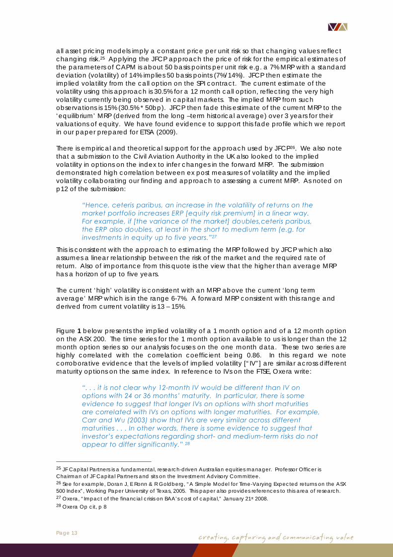
This is consistent with the approach to estimating the MRP followed by JFCP which also assumes a linear relationship between the risk of the market and the required rate of return. Also of importance from this quote is the view that the higher than average MRP has a horizon of up to five years. The current ‘high’ volatility is consistent with an MRP above the current ‘long term average’ MRP which is in the range 6-7%. A forward MRP consistent with this range and derived from current volatility is 13 – 15%. Figure 1 below presents the implied volatility of a 1 month option and of a 12 month option on the ASX 200. The time series for the 1 month option available to us is longer than the 12 month option series so our analysis focuses on the one month data. These two series are highly correlated with the correlation coefficient being 0.86. In this regard we note corroborative evidence that the levels of implied volatility [“IV”] are similar across different maturity options on the same index. In reference to IVs on the FTSE, Oxera write:

“. . . it is not clear why 12-month IV would be different than IV on options with 24 or 36 months’ maturity. In particular, there is some evidence to suggest that longer IVs on options with short maturities are correlated with IVs on options with longer maturities. For example, Carr and Wu (2003) show that IVs are very similar across different maturities . . . In other words, there is some evidence to suggest that investor’s expectations regarding short- and medium-term risks do not appear to differ significantly.” 28

25 JF Capital Partners is a fundamental, research-driven Australian equities manager. Professor Officer is Chairman of JF Capital Partners and sits on the Investment Advisory Committee. 26 See for example, Doran J, E Ronn & R Goldberg, “A Simple Model for Time-Varying Expected returns on the ASX 500 Index”, Working Paper University of Texas, 2005. This paper also provides references to this area of research. 27 Oxera, “Impact of the financial crisis on BAA’s cost of capital,” January 21st 2008. 28 Oxera Op cit, p 8

The increase in volatility since the commencement of the so-called global financial crisis is evident in Figure 1 from the period commencing around August 2007. Although there has been some decline from the peak, the level is still higher than the history shown in Figure 2 (with the exception of the 1987 crash). Figure 1: Volatility of Stock Market

Volatility of S&P 200

0

10

20

30

40

50

60

Feb-01

May-01

Aug-01

Nov-01

Feb-02

May-02

Aug-02

Nov-02

Feb-03

May-03

Aug-03

Nov-03

Feb-04

May-04

Aug-04

Nov-04

Feb-05

May-05

Aug-05

Nov-05

Feb-06

May-06

Aug-06

Nov-06

Feb-07

May-07

Aug-07

Nov-07

Feb-08

May-08

Aug-08

Nov-08

Feb-09

May-09

%

One Month Call One Year Call 90 day historical vol annualised Source: Bloomberg, VAA analysis Figure 2 shows the 90 day moving average of the standard deviation of the ASX 200 Index. This is highly correlated with the IV (correlation is 0.93) for the period in common. The IV is a forward looking volatility measure while the 90 day moving average is clearly historical. The very high correlation between the two gives us some confidence to look at the much longer historical time series for which to relate the current level of the market and the MRP. Figure 2: Implied Volatility in 1 Month call option on ASX 200

90 Day Moving Volatility of All Ordinaries Accumulation Index

0.0%

0.5%

1.0%

1.5%

2.0%

2.5%

3.0%

3.5%

4.0%

05/1

980

05/1

981

05/1

982

05/1

983

05/1

984

05/1

985

05/1

986

05/1

987

05/1

988

05/1

989

05/1

990

05/1

991

05/1

992

05/1

993

05/1

994

05/1

995

05/1

996

05/1

997

05/1

998

05/1

999

05/2

000

05/2

001

05/2

002

05/2

003

05/2

004

05/2

005

05/2

006

05/2

007

05/2

008

05/2

009

Source: Bloomberg, VAA analysis

As discussed above, the IV can be used to obtain an estimate of the forward MRP. Given the evidence on increased market volatility, it is most likely that the underlying MRP has increased substantially, at least in the shorter term.

The recent and sharp decline in the annual historical MRP (of –46% in 2008)29 can be argued to be a result of lower expected cash flows from businesses, higher risk (therefore a higher required rate of return) or some combination. We are of the view that an increase in risk and consequently the required rate of return is a substantive cause. An increase in risk will lead to a decrease in the capitalized value of the stock market and therefore in the observed market return and a negative observed MRP. In other words there will be an inverse relationship between risk and observed market return. This was also found in US data by Giot (2005).30 If the high correlation between the IV and the 90 day moving average of historical volatility held prior to 2001 (the commencement of the data in Figure 1), and we have no reason to believe otherwise, then the historical relationship between implied market risk and return can be observed from an historical time series. Figure 3 illustrates the historical relationship between the 90 day moving average of the return on the All Ordinaries Index and the standard deviation calculated in the same way. As is apparent, there is a negative relationship and the correlation coefficient is -0.53. Figure 3: Historical Market Return and Risk

90 Day Moving Average Market Return V Market Risk

-1.0%

-0.5%

0.0%

0.5%

1.0%

1.5%

2.0%

2.5%

3.0%

3.5%

4.0%

9/05

/198

0

9/05

/198

1

9/05

/198

2

9/05

/198

3

9/05

/198

4

9/05

/198

5

9/05

/198

6

9/05

/198

7

9/05

/198

8

9/05

/198

9

9/05

/199

0

9/05

/199

1

9/05

/199

2

9/05

/199

3

9/05

/199

4

9/05

/199

5

9/05

/199

6

9/05

/199

7

9/05

/199

8

9/05

/199

9

9/05

/200

0

9/05

/200

1

9/05

/200

2

9/05

/200

3

9/05

/200

4

9/05

/200

5

9/05

/200

6

9/05

/200

7

9/05

/200

8

9/05

/200

9

90 Day MA Return 90 Day MA Volat ility

Source: Bloomberg, VAA analysis Given the strong relationship between the forward and backward looking measures of risk and this historical relationship between market return and risk, we have greater confidence that a forward MRP can be derived from the IV. As also noted above, the current MRP estimated from the IV falls in the range 13 – 15% compared with to the 6 – 7% long term average range. If the 6.5% selected by the AER is used to represent the mean MRP then the current MRP from the IV is 14% (6.5%/14% * 30.5%). This is, in our view, a high upper bound of the MRP and can be interpreted as a short to medium term view of the MRP. It is at least a one year view because the IV was derived from a one year maturing call option. Our research has confirmed that it may

29 See Officer & Bishop (2009) Figure 1 30 See Giot, Pierre, “Relationship Between Implied Volatility Indexes and Stock Index Returns,” Journal of Portfolio Management, Spring 2005, pp 92 - 100

take 3 years before the market capitalisation changes to reflect the long term risk adjusted value.31 It implies an MRP above the current ‘equilibrium rate’ or ‘long term average’ being used by regulators. While we are not advocating this approach to estimating an MRP at this time, we make the point that the 6.0% widely used by regulators in the past, and also the 6.5% determined by the AER recently, is clearly below the prevailing shorter term and medium term forward MRP. We do not advocate a move to a double digit MRP at this time however we recommend the use of 7% as the most appropriate long term view to apply under current conditions. If the MRP being considered was for the regulatory period for the Australia Post determination then we would recommend a higher rate. Implied MRP from debt spreads

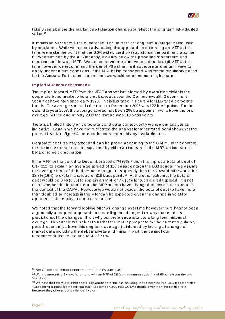
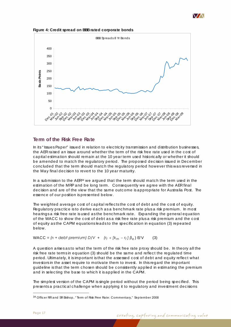
The implied forward MRP from the JFCP analysis is reinforced by examining yields in the corporate bond market where credit spreads over the Commonwealth Government Securities have risen since early 1970. This is illustrated in Figure 4 for BBB rated corporate bonds. The average spread in the data to December 2006 was 122 basis points. For the calendar year 2008, the average spread has been 295 basis points – well above the prior average. At the end of May 2009 the spread was 319 basis points. There is a limited history on corporate bond data consequently we see our analysis as indicative. Equally we have not replicated the analysis for other rated bonds however the pattern is similar. Figure 4 presents the most recent history available to us. Corporate debt is a risky asset and can be priced according to the CAPM. In this context, the rise in the spread can be explained by either an increase in the MRP, an increase in beta or some combination. If the MRP for the period to December 2006 is 7% (6%)32 then this implies a beta of debt of 0.17 (0.2) to explain an average spread of 120 basis points on the BBB bonds. If we assume the average beta of debt does not change subsequently then the forward MRP would be 18.8% (16%) to explain a spread of 319 basis points33. At the other extreme, the beta of debt would be 0.46 (0.53) to explain an MRP of 7% (6%) for such a credit spread. It is not clear whether the beta of debt, the MRP or both have changed to explain the spread in the context of the CAPM. However we would not expect the beta of debt to have more than doubled so increase in the MRP can be expected given the change in volatility apparent in the equity and options markets. We noted that the forward looking MRP will change over time however there has not been a generally accepted approach to modelling the changes in a way that enables predictions of the changes. This is why our preference is to use a long term historical average. Nevertheless it is clear to us that the MRP appropriate for the current regulatory period is currently above this long term average (reinforced by looking at a range of market data including the debt markets) and this is, in part, the basis of our recommendation to use and MRP of 7.0%.

31 See Officer and Bishop paper prepared for ETSA June 2009 32 We are presenting 2 views here – one with an MRP of 7% (our recommendation) and 6% which was the prior ‘standard’. 33 We note that there are other partial explanations for the rise including that presented in a CEG report entitled “Establishing a proxy for the risk free rate” September 2008 that CGS yields are lower than the risk free rate because they offer a ‘convenience’ factor.

Figure 4: Credit spread on BBB rated corporate bonds

BBB Spreads 8 Yr Bonds

0

50

100

150

200

250

300

350

400

Dec-01

Mar-02

Jun-02

Sep-02

Dec-02

Mar-03

Jun-03

Sep-03

Dec-03

Mar-04

Jun-04

Sep-04

Dec-04

Mar-05

Jun-05

Sep-05

Dec-05

Mar-06

Jun-06

Sep-06

Dec-06

Mar-07

Jun-07

Sep-07

Dec-07

Mar-08

Jun-08

Sep-08

Dec-08

Mar-09

Basis

Poi

nts

Term of the Risk Free Rate In its “Issues Paper” issued in relation to electricity transmission and distribution businesses, the AER raised an issue around whether the term of the risk free rate used in the cost of capital estimation should remain at the 10 year term used historically or whether it should be amended to match the regulatory period. The proposed decision issued in December concluded that the term should match the regulatory period however this was reversed in the May final decision to revert to the 10 year maturity. In a submission to the AER34 we argued that the term should match the term used in the estimation of the MRP and be long term. Consequently we agree with the AER final decision and are of the view that the same outcome is appropriate for Australia Post. The essence of our position is presented below. The weighted average cost of capital reflects the cost of debt and the cost of equity. Regulatory practice is to derive each as a benchmark rate plus a risk premium. In most hearings a risk free rate is used as the benchmark rate. Expanding the general equation of the WACC to show the cost of debt as a risk free rate plus a risk premium and the cost of equity as the CAPM equations leads to the specification in equation (3) repeated below. WACC = (rf + debt premium) D/V + efmf β]rk[r( −+ ) E/V (3) A question arises as to what the term of the risk free rate proxy should be. In theory all the risk free rate terms in equation (3) should be the same and reflect the regulated time period. Ultimately, it is important is that the assessed cost of debt and equity reflect what investors in the asset require to motivate them to invest. In this regard the important guideline is that the term chosen should be consistently applied in estimating the premium and in selecting the base to which it is applied in the CAPM. The simplest version of the CAPM is single period without the period being specified. This presents a practical challenge when applying it to regulatory and investment decisions 34 Officer RR and SR Bishop, “Term of Risk Free Rate: Commentary,” September 2008

that are multi-period and of different maturity. Consequently we have to look beyond the CAPM for guidance on its practical application – particularly for selecting an appropriate maturity for the proxy for the risk free rate. Given the CAPM is a one period pricing model then conceptually the appropriate period is the price setter’s horizon. This is hard to discern. However typically there is usually an implicit assumption of a match between the asset life and investor’s planning horizon. Ideally, the maturity of the CAPM should be the maturity of the planning period for which the CAPM is to be used to estimate an expected or required return. This means that if the planning horizon is a long term investment then a long term government bond is the appropriate maturity to use. Since Australia Post’s asset base is largely long term then we deduce that the cost of capital should also be long term. This point is consistent with the general guideline that firms should match the length of their financing maturity with the life of the asset. The notion applies to financing with debt as well as equity. In addition to matching the investors’ horizon with the asset horizon it minimises:

• roll over risk, the risk of not being able to raise the capital at all. Recent examples are Centro Properties and Babcock and Brown who could raise debt at the time of roll-over – shareholders in these companies experiencing a very high cost as a result of this;

• transaction costs associated with raising capital, and • interest rate changes that can cause profitability to be different from what was

expected and expose the business to ‘bankruptcy’ costs. Given the long term nature of the underlying assets and the relative depth and liquidity of the ten year market, we support the use of a ten year maturing proxy for the risk free rate. This is our recommendation and practice in the absence of regulation. To change this recommendation would require the present value of the benefits to be greater than the present value of the costs. The argument against appears to be that presented by Davis35 and Lally36. They commence with the view that the regulatory period is every 5 years (in the distribution and transmission environment which was the context of that regulatory decision). In these determinations the risk free rate is set every five years. They also note that the term structure of CGS is usually upward sloping so the yield on a 10 year bond is higher than that for a 5 year bond. As we understand the argument, it is that the 10 year rate provides compensation for risk for holding a bond for 10 years rather than 5. Thus the use of the 10 year rate in regulatory hearings provides a reward for risk (this difference in the yield of a 10 and 5 year maturing CGS) that the regulated firms do not bear. Our analysis of 10 year CGS compared with 5 year CGS shows that the 10 year rate was on average 18 basis points higher than the 5 year rate. However this means that if the risk free rate was changed to the 5 year yield on CGS then the MRP would have to be adjusted upwards to reflect this difference as well i.e. there is a need for consistency in the way the MRP is measured and the way the risk free rate is measured. Consequently for an asset with a beta of 1 there would be no effect of changing to a 5 year rate compared with a 10 year rate. For assets with betas close to one, any difference is immaterial. The same argument applies if a view was expressed that the term of the risk free rate be changed to 3 years for Australia Post to match the regulatory period. It would be necessary to adjust the MRP accordingly. The readily available data history for 3 year

35 Davis K, Report on risk free interest rate and equity and debt beta determination in the WACC, Prepared for the ACCC, August 2003 36 Lally M, “Determining the risk free rate for regulated companies,” Prepared for ACCC, August 2002.

maturing CGS is shorter than that for 5 year maturing bonds. Data is readily available from the RBA website for the period June 1992 to March 2009. The average difference between 3 year and 10 year bonds for the period is 48 basis points compared with a difference of 18 basis points for 10 year less 5 year maturing bonds over the same period. This suggests the MRP would need an increase of circa 50 basis points if the term of the risk free rate was reduced from 10 to 3 years. We note that after considering all argument, the AER reversed its proposed position to use a 5 year term to revert to the 10 year maturity on the risk free rate. Given this outcome, we do not advance the argument further as we considered the pressure to move to a maturity that matches the regulatory period to be inappropriate in the first place. We were concerned that the AER was of the view that the regulated firms should be financed with 5 year maturing debt as appeared in a statement on page 31 (highlighted below):

“. . . financing strategy is and should be at the discretion of the regulated entity. Provided the regulator commits to resetting interest rates (and cash flows) at the end of the regulatory period, and the firm refinances in the specified averaging period, the exposure to interest rate risk will be minimised to the greatest extent possible” [emphasis added).

Refinancing every 5 (or 3) years would expose Australia Post to significant roll-over risk arising from extending a mismatch between maturing of assets and maturity of financing and would certainly make the present value of the expected costs of moving to a 5 (or 3) year maturing CGS well above the very small benefit of such a change. We certainly do not encourage the ACCC to consider selecting a risk free rate with the same maturity as the Australia Post regulatory period. To change it would be necessary to hold the view that:

• There is an active and deep market for the regulatory period proxy for the risk free rate to ensure the MRP can be re-estimated over the long term and ‘observed’ yields are reflective of a risk free return with minimal other premiums e.g. for lack of marketability;

• The financing transactions costs that may be imposed on regulated firms are not higher than under current arrangements (ceteris paribus);

• The roll-over risk is not higher as a result of ‘going to market’ more frequently than other arrangements under a ten year financing regime;

• The term structure is, on average, upward sloping from the regulatory period to ten year maturities and passing on the financing risk and transactions cost to consumers does not dampen demand arising from this;

• The market risk premium is re-estimated using observed historical market returns and the observed yield on the regulatory period Commonwealth Bond.

We have not seen any evidence presented by those advocating a change from the ten year rate to the regulatory period rate that shows that the change would result in better pricing decisions such that application of the present value principle would yield a closer to zero answer under a regulatory period regime than a ten year regime, all costs and benefits appropriately considered. Consequently we see no reason the change from the yield on the 10 year risk free proxy as the basis for the risk free rate.

Interaction between Spot Rates and Average Rates in the CAPM37 Introduction and Summary

When estimating the cost of debt and cost of equity for input to a WACC, general practice is to use a spot rate for the cost of debt, a spot rate for the risk free rate in the CAPM but an average MRP to estimate the cost of equity. This means that there is a spot risk premium for debt but an average risk premium for equity. Under current circumstances, where the risk spread on debt is historically very high, it is feasible for a mechanical estimation of the cost of debt to be higher than the cost of equity – certainly a substantial narrowing of the two risk margins. A cost of debt higher than the cost of equity is a nonsensical outcome. The issue arises essentially because the use of a spot rate for the risk free rate and an MRP based on the historical average will underestimate the cost of equity under current conditions. Expanding, there are three possible outcomes arising from combining estimates of the risk free rate and MRP determined under different conditions:

a) if the MRP and Rf are both estimated in current market conditions, then the estimated cost of equity would reflect the likely cost of equity over the next regulatory period. This is likely to be much higher than the long term given our estimate of the current MRP following the JFCP approach;

b) if the MRP and Rf are both estimated over a long term, or reflect, a more

“normal” period, then they will result in a cost of equity that is comparable to the long run cost of equity. This will be below the current required return to equity;

c) if the MRP is based on a long term average and the Rf is set reflecting current

conditions where Rf is at abnormally low levels then the resulting cost of equity will be set below average or normal market conditions. It will be well below what is likely to be required in the current market for returns on equity. This appears to be the approach adopted by the AER in its final determination.

Having regard to the conclusion in paragraph (c) above, we do not consider that such an estimate is likely to provide an unbiased value for the current cost of capital for a company. We do not think that current market conditions are requiring a below average cost of capital, in fact, quite the reverse when we look at the discount being required for rights and similar attempts at raising equity capital. Analysis

Our preferred approach is to use spot estimates of the risk free rate, debt spreads and the market risk premium so that the resulting WACC reflects the current view of a required return until the next regulatory price determination i.e. approach a) above. The challenging parameter to estimate is the current forward looking MRP. We noted above the method that uses the implied volatility in options on the market index is one approach to guide such an estimate. As we also noted, this is above the historical average MRP and is also consistent with the high required yields on debt. There is still a challenge in obtaining a defensible estimate derived from a widely agree and accepted method however the direction of the current MRP is very clear and above the long term average.

37 This section draws upon a paper prepared by R Officer, “Expert Report prepared in respect of certain matters arising from the AER’s New South Wales Draft Distribution Determination 2009-10 to 2013-14” January 2009, prepared for Energy Australia.

An issue for establishing a WACC for Australia Post arises if an average MRP is used in conjunction with the current low risk free rate (approach c) above. We now address the matter raised in the introduction after presenting the historical behaviour of the yield on 10 year CGS for context. The current yield on 10 year CGS is near the lowest level in recent years. Figure 5 displays the historical and average yield on 10 year maturing CGS since July 1982. July 1982 was chosen to display the series as it corresponds with a period of ‘freeing up’ the trading in CGS. There were numerous changes occurring in controls on interest rates and the market for CGS in this period including38:

• quantitative lending controls over the Banks were largely removed in June 1982;

• the savings bank specified asset requirement was reduced in August 1984; • maturity controls were abolished in August 1984; • the prime assets ratio (PAR) replaced the liquid government securities (LGS)

convention in May 1985; • the introduction of a tender system for CGS in 1982; • removal of Loan Council control on borrowing by ‘market’ public authorise for

large semi government authorities in July 1983; • abolition of minimum holdings of government securities by life companies and

superannuation funds in September 1984. Consequently we present a view that there was a largely unfettered market for these securities post the early 1980s. Figure 5: Historical Yield on 10 Year Commonwealth Government Securities

0.00

2.00

4.00

6.00

8.00

10.00

12.00

14.00

16.00

18.00

Jul-8

2Ju

l-83

Jul-8

4Ju

l-85

Jul-8

6Ju

l-87

Jul-8

8Ju

l-89

Jul-9

0Ju

l-91

Jul-9

2Ju

l-93

Jul-9

4Ju

l-95

Jul-9

6Ju

l-97

Jul-9

8Ju

l-99

Jul-0

0Ju

l-01

Jul-0

2Ju

l-03

Jul-0

4Ju

l-05

Jul-0

6Ju

l-07

Jul-0

8

%

The critical question, considered below, is whether it is appropriate for the MRP and Rf,t (the risk free rate at point of time t) to be estimated over different periods of time, or during different market conditions. In theory, the task for estimating Rf,t is made easy because it is assumed constant and ‘known for certain’ at the time the rate is set. In practice there is no observed Rf,t, instead the yield on a 10 year Commonwealth Government Bond/Security (“CGS”) is used as the surrogate. This yield should theoretically be taken from the CGS as close as practical to the start of the regulated period. It is only in circumstances where this yield is determined to be unrepresentative for the time period or, more relevantly, the current yield is inconsistent with the estimation of the other parameters used to estimate the cost of

38 Source: 1999 Special Article - Institutional Arrangements and Policy, www.abs.gov.au/AUSSTATS/[email protected]/featurearticlesbyCatalogue/338F7A49F638369FCA256F2A00073471?OpenDocument#

capital estimate that an alternative estimate such as the average yield over a particular time period may be justified. The rate should reflect all the conditions that give rise to the rate or yield on the government security for that time period. The task is not so simple for the E(MRPt) because theory does not give us clear guidance as to how we should estimate the ‘E’ of the MRP. We know the variable is stochastic. If it was a constant it would not attract any risk premium and it would be set at zero. However, the process by which ‘E’ is formed in the market place is not clear. Implicitly it is often assumed that ‘E’ will reflect the long term average of the MRP but this is a naive forecast and evidence is mounting, as noted earlier, that better forecasts can be made reflecting current economic conditions. In the circumstances, it is tempting to set the Rf,t to reflect current rates and set the E(MRPt) to reflect the long term average, on the basis that getting one of the variables as close to the relevant time period is better than neither. This would be a reasonable approach if the two variables were independent of each other, i.e. the value of one variable was not related to the value of the other variable. However, by construction we know this is unlikely since MRP= E(Rm) – Rf and that both variables contain Rf. Moreover, if they (MRP and Rf) were negatively related which seems likely given the construction of MRP, then periods of low Rf would be associated with high MRP and conversely. Further, there is the likelihood of a negative economic relationship between Rf and E(Rm) because, for example if the central bank wished to ‘slow the economy down’ resulting in lower equity returns, it would do so by increasing interest rates (Rf) and conversely. The consequence is that when the Rf is at a ‘low level’ (relative to ‘normal’) the estimate of MRP is likely to be at a ‘high level’. For example, when the financial markets are in a ‘bear phase’ as they have been, the correlation between the variables Rft and Rmt and similarly Rf,t and MRPt is likely to be negative – low values of Rft are associated with high levels of E(MRPt) and conversely. For example if we define ‘bull’ and ‘bear’ markets as those for which Rmt is above average and below average respectively then the correlation between the variables goes from slightly positive to strongly negative as illustrated in the table below. Table 3: Correlation between Risk Free Rate and MRP Period Bull Market Bear Market Rm above the average Rm below the average 1883 to 2008 0.29 -0.55 1958 to 2008 0.23 -0.40

If MRP is set at an ‘average or normal level,’ which is representative of a long run mean or expected value over the long term, and Rft is at a low level, such as exists at the moment, this will under-estimate the return to equity E(Re,t) and penalise the regulated entity, and conversely when Rf is at a ‘high level’. Therefore, setting the parameters on the basis of different time periods when one is set at the current time may lead to greater error than if they were both set on the basis of the same or ‘normal’ time period even though this is not representative of the current period. The extent of the possible measurement error depends on the degree of negative correlation between the two variables (either MRP and Rf or Rm and Rf). The greater the correlation the greater the chance of error in the MRP estimate when the variables are measured at different time periods. Ideally, we would estimate both variables at the current time period but if the measurement error for estimating current MRP was great relative to approximating a current cost of capital by a ‘long term average’ then we might be better estimating both variables and therefore the cost of capital as a ‘long term average’.

If the difficulties in estimating a current MRP are such that the estimates are unreliable and create additional uncertainty then a ‘long term average’ or more ‘normal’ time period for estimating the MRP is likely to be more appropriate. In these circumstances it is likely that the measurement error of the estimate of the company’s cost of capital will be reduced by adopting a similar time period for estimating Rf, that is, a ‘long term average’ . If, on the other hand, we believe a current estimate of MRP can be obtained that is more representative of current conditions and does not create the unreliability and uncertainty mentioned in the previous paragraph then it might be determined that current estimates of both MRP and Rf might be more appropriate. We identified such an approach using options on a market index earlier. There is little doubt that current levels of risk are high and that required returns, reflecting this risk, are greater than ‘normal’. One only has to look at the ‘spreads’ on corporate bonds and like instruments to see clear evidence of greater required returns reflecting greater risk. We know that the MRP cannot be constant but we have limited empirical evidence on the relevant parameters that determine its values, as a consequence, at a practical or operational level one is obliged to use methods that give some semblance of approximating reality even if there is limited evidence supporting such approaches. It is in recognition of this that JF Capital Partners, a fund manager with a very rigorous valuation approach to stock selection, has chosen such a model or approach. Further, the current experience and estimates clearly illustrate the inverse relationship between the Rf and the MRP; interest rates on 10 year government bonds are at 50 year lows and MRP’s are at record high levels. Noting the comments above, in estimating the parameters of the CAPM and having regard to the evidence of current MRP and Rf, there are the three possible outcomes described earlier. We do not think that current market conditions are requiring a below average cost of capital, in fact, quite the reverse when we look at the discount being required for rights and similar attempts at raising equity capital.

Impact of Imputation Tax on Australia Post An imputation tax system was introduced in Australia from July 1 1987. A key purpose of the imputation system was to remove the tax bias against equity income in the prior classical tax system and place it on the same tax footing as debt income. The imputation system removed the double taxation of dividend income under a classical tax system for Australian Resident Taxpayers. The classical system taxed equity income at the corporate level and then again at the personal level. Under the imputation system, corporate tax can be viewed as a collection of personal tax for those subsequently claiming the imputation tax benefits. The Australian system has since been modified over time in a number of ways. Some relevant changes are:

• A corporate tax on superannuation funds was introduced from 1st July, 1988 to enable them to use imputation tax benefits and to remove any disincentive to invest in companies paying imputation benefits;

• The introduction of a 45 day holding period around the distribution of franking tax credits in 1997 which imposes additional ‘cost’ on trading in credits;

• A move to a rebate rather than tax credit system in July 2000 which enables domestic tax exempt and low taxed residents to now fully access imputation benefits.

An outcome of the imputation system is a differential effect across some shareholder groups. The ‘beneficiaries’ are, in the broad, individuals and superannuation funds whereas foreign investors and tax-exempt shareholders (historically) did not gain directly from the change. As a result, the net dollar return after tax these different shareholders groups earn can differ. The term “gamma” has been used widely to reflect the value of a dollar of imputation tax benefits. It is used to adjust either the tax rate in after cash flow estimation or to the cost of capital when undertaking project or enterprise valuations or when assessing regulatory revenue requirements. However we do not use gamma but rather a component of it to adjust for the impact of imputation tax benefits on ‘measures’ company or market returns. There are three milestones in the life of an imputation tax benefit as described by Hathaway and Officer (2004).

1. It is created when company tax is paid; 2. It is distributed when company tax is paid to shareholders as an attachment to

dividends; 3. It is redeemed when shareholders claim the rebate and enjoy the tax benefit.

Common usage is to define gamma (γ) as the value of a dollar of imputation tax benefit when it is created. A dollar of imputation tax created will be retained (and tracked as a “FAB” - franking account balance – until it is distributed by way of an attachment to a dividend. The imputation tax benefits are of direct interest to shareholders once they are distributed. Thus when looking at the return shareholders receive from their investment over a particular period, we are interested in capital gains, dividends and the imputation tax benefits attached to dividends.39 The relationship between gamma and the value of imputation tax benefits distributed is captured in equation (7).

39 Any value to imputation tax benefits retained will be reflected in the share price through an anticipation of when they may be distributed and their value at this time.

γ = F x φ (7)

Where F is the proportion of imputation tax benefits created that are distributed (attached to dividends)

φ is the value of an imputation tax benefit that has been distributed. We define this to be the value on the day that the stock becomes ex dividend. Dividend drop-off studies estimate a value for φ.

Regulatory bodies have used a value of 0.5 for gamma to adjust statutory tax paid to reflect the amount that is distributed and used by shareholders however the most recent decision by the AER in May 2009 used a value of 0.65 for gamma. It is assumed that the intention of the regulatory approach to pricing for Australia Post is to set a revenue requirement that covers all operating costs, taxes, a return of capital (depreciation) and a commercial return on capital. Australia Post is owned by the Australian Government but is subject to corporate tax. To ensure the capital invested in Australia Post earns a commercial rate of return, this tax must be recognised as a cost of business and so the pricing of regulated services must reflect this cost. In this regard, corporate tax is no different to any other cost or tax imposed on Australia Post. Unlike the privately owned Distribution and Transmission businesses falling under the AER jurisdiction, Australia Post does not distribute imputation credits along with dividends and the shareholders do not claim imputation tax benefits as a personal tax rebate. Thus there is no imputation tax benefit for shareholders and the effective corporate tax rate is generally the statutory rate. Consequently both F and φ are zero for Australia Post therefore gamma is also zero. If the WACC or costs of Australia Post are adjusted on the grounds that gamma is non-zero then Australia Post will not earn a commercial rate of return on its capital. We would expect that if the Government, as shareholder, wanted to place Australia Post on the same footing as privately owned businesses then it would reduce the corporate tax rate. It has not. Since it has not reduced the tax rate then Australia post will not earn a commercial cost of capital if a gamma other than zero is employed in regulatory price setting.

Beta of Equity The cost of equity is generally derived from the CAPM where the beta of equity captures the risk of equity that is rewarded by the market. Ideally it is a forward estimate but typically it is estimated from the historical relationship of the return on equity relative to the return on a market index. Since Australia Post is not a listed company, the beta cannot be estimated directly. Consequently it is estimated by reference to comparable companies. To maintain consistency with the process of estimating betas in the past, we have essentially replicated the process followed by Capital Partners in 2005 to estimate a cost of capital for Australia Post. This involved estimating an asset beta from the equity beta of comparable companies for each major business unit and determining a weighted average of these for the Australia Post as a whole. The equity beta was assessed by relevering the asset beta at a target gearing of 30%. We have modified the process in one respect as guided by Australia Post. Rather than estimate a beta for each business unit and weight them to obtain an overall beta the comparables were grouped in total to form one overall beta. As it turned out, the overall asset beta was essentially the same under each approach using the most recent data. The beta of assets was derived from the beta of equity of a set of companies considered to be comparable to the Australia Post business activities. The comparable list was updated from the initial Capital Partners work in conjunction with Australia Post. The list is provided in Appendix 2 along with relevant financial and beta related information. It is a wide ranging list of comparables that reflects the diversity of business activities undertaken. The estimation process involved delevering the beta of equity, in turn derived from using ordinary least squares regression of the return on the comparable company against the return on the market. Sixty monthly observations to March 2009 were used in the regression analysis. The underlying relationship used in the levering and delivering process was derived from the following plain vanilla formula:

VE

VD

EDa βββ += (8)

Where: βa = beta of assets βD = beta of debt βE = beta of equity D/V = average gearing E/V = (1 – D/V) The beta of debt was derived by ‘back-solving’ for it from the CAPM based on a debt premium considered appropriate for its credit rating i.e. βD = (credit spread)/ MRP. If the comparable was from another economy then the beta of equity was estimated against an index of the ‘home’ country and the ‘local’ tax rate was used. The derived beta of assets for each business unit comparable set was a weighted average (by Enterprise Value) across all companies.

There were some changes in the comparable set used by Capital Partners due to takeovers, de-listings etc and we added to the list using the same selection logic as followed by Capital Partners to update the set. The outcome is summarised below. Component Current Estimate Prior Estimate Asset Beta 0.78 0.52 Beta Debt 0.15 0.1 Target Gearing 30% 30% Beta of Equity 1.07 0.71 The estimate of a beta of assets for Australia Post is 0.78. Relevering this beta of assets at a target gearing of 30% (as advised by Australia Post) leads to an estimated beta of equity of 1.0 (rounded down). This is similar to a simple weighted average of other (international) listed postal services of 0.97, although above the relevered asset beta of these comparables at 30% gearing which was 0.84. The beta of assets as assessed is higher than the prior estimate. We note that, although not the same set of comparable postal companies, the beta of assets of this group has also risen, from 0.43 to 0.52 from the prior to the current estimate.

Appendix 1: Method of including Imputation Tax Yield in the Historical MRP The imputation tax benefit to include in the index is described in equation (7) below. The adjustment to the index for the value of the tax credits from 1988 forward was estimated as follows:

tt dVFC = Φ.f).T1

T( t

ct

tc−

. . . (7)

Where VFCt is the estimated rate of return from imputation tax benefits in year t for all stocks in the market index

dt is the dividend yield in the index in year t being a capitalised weighted sum of individual company dividend yields

ft is percentage of dividends in the index of market returns that are franked (attract an imputation tax benefit)

φt is the value of a dollar of imputation tax benefit that is distributed (not this is different from gamma

Tct is the statutory corporate tax rate in year t. The dividend yield (dt) for each year was calculated as the difference between the All Ordinaries Accumulation and Price indexes and represents the weighted sum of the dividend yield on each stock included in the index. The percentage of dividends franked (ft) was estimated in two ways. In the first case, data published by the Australian Tax Office on total dividends paid, broken in to franked and unfranked provided an estimate for each year from 1993 to 2008. A simple average of this percentage was assumed to apply in the years 1988 to 1992 for which tax statistics are not available. These data apply to all companies submitting tax returns which may differ from an estimate based only on the stocks included in the All Ordinaries Index. In the second case, the franked dividend percentage for each stock in the index for each year was extracted from Bloomberg data and weighted by the stocks weight in the index. This better aligns the franking tax credit with the dividend yield in the index. The value of a dollar of imputation tax benefit distributed (φt) was not formally estimated. Instead we chose values to illustrate the impact of an imputation tax adjustment. In particular the values of 0, 0.5, 0.65 and 1 were selected. Zero is a natural outcome of excluding imputation tax benefits, 0.5 is the value used in a number of regulatory price determinations for gamma (here it is used as the value of a dollar of imputation tax credit distributed), 0.65 was the value ascribed to such credits in its most recent WACC parameter determination (May 2009) and 1 is the other extreme (and unlikely40)) value. The corporate tax rate in each year (Tct) used was the statutory rate applicable from July of the year examined. The corporate tax rate was obtained from the Australian Tax Office website. There are a number of potential inaccuracies here that we have ignored. One is the fact that the market rate of return was based on a calendar year whereas the tax rate is based on a financial year. This may lead to a small inaccuracy in years when the tax rate changed

40 Unlikely at least because there is a time delay between the distribution of the imputation tax benefit and the ‘cash flow’ benefit to the ultimate shareholder.

Estimates of the VFC for the thirteen years from 1993 to 2005 indicate an average value for the VFC of 85 basis points if the value of a dollar of franking credits distributed (φ) is 0.5. This would suggest an increase in the market rate of return for the period by an average of 0.85%. For example if the MRP for the period or the expected MRP was 6% then it should be adjusted to 6.85% for the effective value of the franking credits. This is not a large amount and well within the range of standard measurement errors one might expect from estimates of the MRP. However, on the basis of such an estimate, given a value of 0.5 for imputation tax credits distributed, in our view an MRP of 7% is more justifiable than one of 6%. Added strength for this view arises from most historical averages (across different periods) being greater than 6%. Research subsequent to Officer, by Brailsford et al41, revised the market return data used by Officer prior to 1958. We do not have access to this data. Consequently we have used the summary data from Brailsford et al to estimate the summary information in Table 1 for the periods commencing 1883 whereas we used our own data sources for the period commencing 195842. The market returns, and consequently the MRP, for the original Officer series are higher for the period 1883 to 1958 as implied by the data in Table 1.43

41 Op cit 42 We broke the entire period into 1883 to 1957 and 1958 to the end year. Brailsford et al summary data was used for the former period and Officer and Bishop data used for the latter period. 43 See both Brailsford and Officer and Bishop for further comments.

Appendix 2: Comparable Analysis for Estimating Beta

Company NameValuation Date:

Market Cap Last Reported DebtEnterprise

ValueAve D/V

RatioBeta of Debt

(Ave)Observed Beta

of Equity Beta of Assetsm AUD m AUD m AUD 3 Yrs

Comparable Companies

Stock ExchangesAustralian Stock Exchange 5,295 3,653 8,948 31% 0.17 0.97 0.72Hong Kong Exchanges & Clear 17,295 5 17,300 0% 0.15 1.60 1.60Nyse Euronext 7,687 4,452 12,139 14% 0.11 1.40 1.23

38,387 15% 0.14 1.32 1.18Transaction Processing

Paychex Inc 13,848 - 13,848 0% 0.18 0.85 0.85Deluxe Corp 817 1,211 2,028 43% 0.31 1.97 1.25Equifax Inc 4,716 1,730 6,446 19% 0.15 1.16 0.96Coinstar Inc 1,332 499 1,831 28% 1.16 1.03 1.07

24,153 23% 0.45 1.25 1.03Retail

Woolworths Limited 32,822 2,774 35,596 11% 0.11 0.55 0.50Billabong International Ltd 1,813 483 2,297 12% 0.17 1.10 0.99Reject Shop Ltd/The 283 14 297 3% 0.17 0.88 0.86

38,190 8% 0.84 0.78

Property DevelopmentWestfield Group 23,470 20,989 44,459 36% 0.11 0.47 0.34Peet Ltd 379 274 653 23% 0.17 1.31 1.04Australand Property Group 729 1,567 2,297 55% 0.17 1.79 0.90Port Bouvard Ltd 61 64 124 15% 0.17 1.50 1.29

47,534 32% 0.16 1.27 0.90

Listed Postal ServicesTNT NV 9,118 4,437 13,555 20% 0.15 0.94 0.78Deutsche Post Ag-Reg 20,883 8,112 28,996 45% 0.15 1.09 0.67Singapore Post Ltd 1,385 240 1,625 13% 0.07 0.57 0.51Oesterreichische Post Ag 2,801 294 3,095 8% 0.15 0.17 0.17

47,271 21% 0.13 0.69 0.53

Express Parcel DeliveryUnited Parcel Service-Cl B 78,299 14,008 92,308 11% 0.07 0.85 0.76Fedex Corp 22,985 2,101 25,087 7% 0.18 0.89 0.85Yamato Holdings Co Ltd 6,523 1,561 8,084 15% 0.07 0.92 0.79Freightways Ltd 309 160 469 26% 0.15 0.90 0.70Blue Dart Express Limited 278 - 278 0% 0.15 0.67 0.67

126,225 12% 0.12 0.85 0.75

Australian InfrastructureOrigin Energy Limited 13,453 3,379 16,831 26% 0.15 0.56 0.45AGL Energy Ltd 6,579 2,102 8,680 - 0.17 0.44 0.38Transurban Group 5,233 3,744 8,977 38% 0.17 0.44 0.34Macquarie Infrastructure Group 2,958 2,428 5,387 30% 0.17 1.05 0.78SP Ausnet 1,919 3,671 5,590 57% 0.11 0.09 0.10APA Group 1,371 3,111 4,482 60% 0.17 0.75 0.40Duet Group 1,222 4,870 6,092 74% 0.15 0.47 0.23Spark Infrastructure Group 999 1,724 2,723 53% 0.17 0.35 0.26Envestra Limited 584 1,963 2,548 71% 0.15 0.56 0.27Australian Infrastructure Fund 573 130 703 4% 0.17 1.15 1.10Challenger Infrastructure-A 540 1,879 2,418 - 0.17 0.25 0.20Transfield Services Infrasture 302 773 1,075 - 0.17 1.10 0.45Hastings Diversified Utilities 139 442 580 41% 0.17 0.03 0.09

66,087 45% 0.16 0.56 0.39

Express Parcel DeliveryUnited Parcel Service-Cl B 78,299 14,008 92,308 11% 0.07 0.85 0.76Fedex Corp 22,985 2,101 25,087 7% 0.18 0.89 0.85Yamato Holdings Co Ltd 6,523 1,561 8,084 15% 0.07 0.92 0.79Freightways Ltd 309 160 469 26% 0.15 0.90 0.70Blue Dart Express Limited 278 - 278 0% 0.15 0.67 0.67

126,225 12% 0.12 0.85 0.75Australian Logistics

Cti Logistics Ltd 29 8 36 30% 0.17 1.17 0.87K & S Corporation Limited 161 70 230 22% 0.17 0.40 0.35Toll Holdings Limited 4,271 1,622 5,892 30% 0.17 0.65 0.51Wridgways Australia Limited 61 - 61 0% 0.17 0.86 0.86

6,220 21% 0.17 0.77 0.64International Logistics

D. Logistics Ag 105 151 256 52% 0.15 1.17 0.64Wincanton Plc 358 374 732 11% 0.15 1.27 1.15Logwin Ag 264 392 656 45% 0.46 1.35 0.95Hub Group Inc-Cl A 1,111 - 1,111 0% 0.18 1.17 1.17

2,755 27% 0.23 1.24 0.98

Average Asset Beta 0.79

Selected References AER, “Statement of Regulatory Intent on the Revised WACC Parameters (Distribution): Explanatory Statement”, December 2008 AER, “Review if the Weighted Average Cost of Capital WACC) Parameters: Proposed”, December 2008 AER, “Electricity transmission and distribution network service providers: Review of the weighted average cost of capital (WACC) parameters” Final Decision May 2009 Bishop SR & RR Officer (2008), “Market Risk Premium: A Review Paper”, Value Adviser Associates, August 2008 Bishop SR & RR Officer (2009), “Market Risk Premium: Further Comments”, Value Adviser Associates, January 2009 Bollerslev T & H. Zhou, “Expected Stock Returns and Variance Risk Premia”, Working Paper, September 2006 Brailsford et al (2008): Brailsford T, J Handley & K Maheswaran, “Re-examination of the historical equity risk premium in Australia,” Accounting and Finance, 48, (2008) pp 73-97 CEG, “Establishing a proxy for the risk free rate: A report for the APIA, ENA and Grid Australia,” Submission to AER, 17 September 2008 CEG: Hird T & D Young (2009), “The Market Risk Premium and Risk Free Rate under the NER and in a Period of Financial Crisis: A report for ETSA”, June 2009 Doran J, E Ronn & R Goldberg, “A Simple Model for Time-Varying Expected returns on the ASX 500 Index”, Working Paper University of Texas, 2005 Stephen Gray and R R Officer, “A review of the market risk premium and commentary on two recent papers” A report prepared for the Energy Networks Association, August 2005 Giot, Pierre, “Relationship Between Implied Volatility Indexes and Stock Index Returns,” Journal of Portfolio Management, Spring 2005, pp 92 - 100 Hathaway N & RR Officer, “The Value of Imputation Tax Credits,” Capital Research, 2004 Officer, R.R., “A Note on the Cost of Capital and Investment Evaluation For Companies Under the Imputation Tax”, Accounting and Finance, November 1988 Officer, R. R. (1989), ‘Rates of Return to Shares, Bond Yields and Inflation Rates: An Historical Perspective’, in Ray Ball, Philip Brown, Frank J. Finn and R. R. Officer(eds.), Share Markets and Portfolio Theory: Readings and Australian Evidence, University of Queensland Press. Officer R R, “The Cost of Capital of a Company Under an Imputation Tax System,” Accounting and Finance Vol 34, 1 (1994) pp1-17 Officer, R.R. & N. Hathaway, “The Value of Imputation Tax Credits”, Pacific basin Finance Conference Paper, New York, 1991 plus updates Oxera “Impact of the financial crisis on BAA’s cost of capital”, January 21

regulatory wacc for australia post wacc for australia... · regulatory wacc for australia post...

Documents