regulatory impact analysis of the final revisions to … · ii epa-452/r-15-007 september 2015...
TRANSCRIPT

Regulatory Impact Analysis of the Final Revisions to the National Ambient Air
Quality Standards for Ground-Level Ozone

ii
EPA-452/R-15-007 September 2015
Regulatory Impact Analysis of the Final Revisions to the National Ambient Air Quality Standards for Ground-Level Ozone
U.S. Environmental Protection Agency
Office of Air and Radiation Office of Air Quality Planning and Standards
Research Triangle Park, NC 27711

iii
CONTACT INFORMATION
This document has been prepared by staff from the Office of Air Quality Planning and
Standards, U.S. Environmental Protection Agency. Questions related to this document should be
addressed to Robin Langdon, U.S. Environmental Protection Agency, Office of Air Quality
Planning and Standards, C439-02, Research Triangle Park, North Carolina 27711 (email:
[email protected]). The docket number for this Regulatory Impact Analysis is EPA-HQ-
OAR-2013-0169.
ACKNOWLEDGEMENTS
In addition to EPA staff from the Office of Air Quality Planning and Standards, personnel from
the Office of Atmospheric Programs, the Office of Transportation and Air Quality, the Office of
Policy Analysis and Review, and the Office of Policy’s National Center for Environmental
Economics contributed data and analysis to this document.

iv
TABLE OF CONTENTS page
LIST OF TABLES ......................................................................................................................... xi
LIST OF FIGURES .......................................................................................................................xx
EXECUTIVE SUMMARY .......................................................................................................ES-1
Overview .............................................................................................................................ES-1 ES.1 Overview of Analytical Approach ....................................................................ES-4
ES.1.1 Establishing the Baseline ..............................................................................ES-5 ES.1.2 Control Strategies and Emissions Reductions ..............................................ES-6
ES.1.2.1 Emissions Reductions from Identified Controls in 2025 ....................ES-7 ES.1.2.2 Emissions Reductions beyond Identified Controls in 2025 ................ES-9 ES.1.2.3 Emissions Reductions beyond Identified Controls for Post-2025 ....ES-10
ES.1.3 Human Health Benefits ..............................................................................ES-11 ES.1.4 Welfare Benefits of Meeting the Primary and Secondary Standards .........ES-13
ES.2 Results of Benefit-Cost Analysis ....................................................................ES-14 ES.3 Improvements between the Proposal and Final RIAs .....................................ES-19 ES.4 Uncertainty .....................................................................................................ES-21 ES.5 References .......................................................................................................ES-21
CHAPTER 1: INTRODUCTION AND BACKGROUND ........................................................ 1-1
Introduction ........................................................................................................................... 1-1 1.1 Background ................................................................................................................ 1-3
1.1.1 National Ambient Air Quality Standards ....................................................... 1-3 1.1.2 Role of Executive Orders in the Regulatory Impact Analysis ........................ 1-3 1.1.3 Illustrative Nature of the Analysis .................................................................. 1-4
1.2 The Need for National Ambient Air Quality Standards ............................................ 1-5 1.3 Overview and Design of the RIA ............................................................................... 1-6
1.3.1 Establishing Attainment with the Current Ozone National Ambient Air Quality Standard ........................................................................................................ 1-6
1.3.2 Establishing the Baseline for Evaluation of Revised and Alternative Standards .................................................................................................................. 1-10
1.3.3 Cost Analysis Approach ............................................................................... 1-12 1.3.4 Human Health Benefits ................................................................................ 1-13 1.3.5 Welfare Benefits of Meeting the Primary and Secondary Standards ........... 1-13
1.4 Updates between the Proposal and Final RIAs ........................................................ 1-13 1.5 Organization of the Regulatory Impact Analysis ..................................................... 1-15 1.6 References ................................................................................................................ 1-16
CHAPTER 2: EMISSIONS, AIR QUALITY MODELING AND ANALYTIC METHODOLOGIES ............................................................................................................ 2-1
Overview ............................................................................................................................... 2-1
v
2.1 Emissions and Air Quality Modeling Platform ......................................................... 2-4 2.2 Projecting Ozone Levels into the Future ................................................................... 2-6
2.2.1 Methods for Calculating Future Year Ozone Design Values ......................... 2-6 2.2.2 Emissions Sensitivity Simulations ................................................................. 2-8 2.2.3 Determining Ozone Response Factors from Emissions Sensitivity
Simulations .............................................................................................................. 2-13 2.2.4 Combining Response from Multiple Sensitivity Runs to Determine Tons
of Emissions Reductions to Meet Various NAAQS Levels .................................... 2-16 2.2.5 Monitoring Sites Excluded from Quantitative Analysis............................... 2-18
2.3 Creating Spatial Surfaces for BenMap .................................................................... 2-20 2.4 Improvements in Emissions and Air Quality for the Final RIA .............................. 2-24
2.4.1 Improvement in Emissions ........................................................................... 2-24 2.4.2 Improvements in Air Quality Modeling ....................................................... 2-26
2.5 References ................................................................................................................ 2-27
APPENDIX 2A: ADDITIONAL AIR QUALITY ANALYSIS AND RESULTS ................. 2A-1
2A.1 2011 Emissions and Air Quality Modeling Platform ...................................... 2A-1 2A.1.1 Photochemical Model Description and Modeling Domain ......................... 2A-1 2A.1.2 Meteorological Inputs, Initial Conditions, and Boundary Conditions ........ 2A-2 2A.1.3 2025 Base Case Emissions Inputs ............................................................... 2A-4 2A.1.4 2011 Model Evaluation for Ozone .............................................................. 2A-8
2A.2 VOC Impact Regions ..................................................................................... 2A-30 2A.3 Monitors Excluded from the Quantitative Analysis ...................................... 2A-30
2A.3.1 Sites without Projections Due to Insufficient Days ................................... 2A-31 2A.3.2 Winter Ozone ............................................................................................. 2A-32 2A.3.3 Monitoring Sites in Rural/Remote Areas of the West and Southwest ...... 2A-33
2A.4 Design Values for All Monitors Included in the Quantitative Analysis ........ 2A-36 2A.5 References ...................................................................................................... 2A-65
CHAPTER 3: CONTROL STRATEGIES AND EMISSIONS REDUCTIONS ....................... 3-1
Overview ............................................................................................................................... 3-1 3.1 The 2025 Control Strategy Scenarios ........................................................................ 3-2
3.1.1 Approach for the Revised Standard of 70 ppb and Alternative Standard of 65 ppb ........................................................................................................................ 3-2
3.1.2 Identified Control Measures ........................................................................... 3-8 3.1.3 Results .......................................................................................................... 3-10
3.2 The Post-2025 Scenario for California .................................................................... 3-17 3.2.1 Creation of the Post-2025 Baseline Scenario for California ........................ 3-17 3.2.2 Approach for Revised Standard of 70 ppb and Alternative Standard of 65
ppb for California ..................................................................................................... 3-20 3.2.3 Results for California.................................................................................... 3-20
3.3 Improvements and Refinements since the Proposal RIA ........................................ 3-24 3.4 Limitations and Uncertainties .................................................................................. 3-26 3.5 References ................................................................................................................ 3-29
vi
APPENDIX 3A: CONTROL STRATEGIES AND EMISSIONS REDUCTIONS ................ 3A-1
Overview ............................................................................................................................ 3A-1 3A.1 Target Emissions Reductions Needed to Create the Baseline, Post-2025
Baseline and Alternatives ............................................................................................... 3A-1 3A.2 Numeric Examples of Calculation Methodology for Changes in Design
Values ......................................................................................................................... 3A-3 3A.3 Types of Control Measures .............................................................................. 3A-4 3A.4 Application of Control Measures in Geographic Areas .................................. 3A-5 3A.5 NOx Control Measures for Non-EGU Point Sources ...................................... 3A-8 3A.6 VOC Control Measures for Non-EGU Point Sources ................................... 3A-14 3A.7 NOx Control Measures for Nonpoint (Area) and Nonroad Sources .............. 3A-15 3A.8 VOC Control Measures for Nonpoint (Area) Sources .................................. 3A-15
CHAPTER 4: ENGINEERING COST ANALYSIS AND ECONOMIC IMPACTS ................ 4-1
Overview ............................................................................................................................... 4-1 4.1 Estimating Engineering Costs .................................................................................... 4-2
4.1.1 Methods and Data ........................................................................................... 4-3 4.1.2 Engineering Cost Estimates for Identified Controls ..................................... 4-10
4.2 The Challenges of Estimating Costs for Unidentified Control Measures ................ 4-16 4.2.1 Impact of Technological Innovation and Diffusion ..................................... 4-18 4.2.2 Learning by Doing ........................................................................................ 4-22 4.2.3 Incomplete Characterization of Available NOx Control Technologies ........ 4-24 4.2.4 Comparing Baseline Emissions and Controls across Ozone NAAQS RIAs
from 1997 to 2014 .................................................................................................... 4-30 4.2.5 Possible Alternative Approaches to Estimate Costs of Unidentified
Control Measures ..................................................................................................... 4-31 4.2.6 Conclusion .................................................................................................... 4-35
4.3 Compliance Cost Estimates for Unidentified Emissions Controls .......................... 4-35 4.3.1 Methods ........................................................................................................ 4-36 4.3.2 Compliance Cost Estimates from Unidentified Controls ............................. 4-40
4.4 Total Compliance Cost Estimates ............................................................................ 4-41 4.5 Economic Impacts .................................................................................................... 4-42
4.5.1 Introduction .................................................................................................. 4-42 4.5.2 Summary of Market Impacts ........................................................................ 4-44
4.6 Differences between the Proposal and Final RIAs .................................................. 4-45 4.7 Uncertainties and Limitations .................................................................................. 4-46 4.8 References ................................................................................................................ 4-48
APPENDIX 4A: ENGINEERING COST ANALYSIS ........................................................... 4A-1
Overview ............................................................................................................................ 4A-1 4A.1 Cost of Identified Controls in Alternative Standards Analyses ....................... 4A-1 4A.2 Alternative Estimates of Costs Associated with Emissions Reductions from
Unidentified Controls ..................................................................................................... 4A-5

vii
4A.3 Alternative Approaches to Estimating the Costs Associated with Emissions Reductions from Unidentified Controls ......................................................................... 4A-7
4A.3.1 Regression Approach ...................................................................................... 4A-7 4A.3.2 Simulation Approach ...................................................................................... 4A-9
CHAPTER 5: QUALITATIVE DISCUSSION OF EMPLOYMENT IMPACTS OF AIR QUALITY ............................................................................................................................. 5-1
Overview ............................................................................................................................... 5-1 5.1 Economic Theory and Employment .......................................................................... 5-1 5.2 Current State of Knowledge Based on the Peer-Reviewed Literature ....................... 5-6
5.2.1 Regulated Sectors ........................................................................................... 5-7 5.2.2 Economy-Wide ............................................................................................... 5-8 5.2.3 Labor Supply Impacts ..................................................................................... 5-8
5.3 Employment Related to Installation and Maintenance of NOx Control Equipment .. 5-9 5.3.1 Employment Resulting from Addition of NOx Controls at EGUs ................. 5-9 5.3.2 Assessment of Employment Impacts for Individual Industrial,
Commercial, and Institutional (ICI) Boilers and Cement Kilns .............................. 5-15 5.4 Conclusion ............................................................................................................... 5-18 5.5 References ................................................................................................................ 5-19
CHAPTER 6: HUMAN HEALTH BENEFITS ANALYSIS APPROACH AND RESULTS .. 6-1
6.1 Summary .................................................................................................................... 6-1 6.2 Overview .................................................................................................................... 6-3 6.3 Updated Methodology Presented in the Proposal and Final RIAs ............................ 6-7 6.4 Human Health Benefits Analysis Methods ................................................................ 6-9
6.4.1 Health Impact Assessment............................................................................ 6-10 6.4.2 Economic Valuation of Health Impacts ........................................................ 6-12 6.4.3 Estimating Benefits for 2025 and Post-2025 Analysis Years....................... 6-13 6.4.4 Benefit-per-ton Estimates for PM2.5 ............................................................. 6-14
6.5 Characterizing Uncertainty ...................................................................................... 6-16 6.5.1 Monte Carlo Assessment .............................................................................. 6-17 6.5.2 Quantitative Analyses Supporting Uncertainty Characterization ................. 6-18 6.5.3 Qualitative Assessment of Uncertainty and Other Analysis Limitations ..... 6-20
6.6 Benefits Analysis Data Inputs .................................................................................. 6-20 6.6.1 Demographic Data ........................................................................................ 6-21 6.6.2 Baseline Incidence and Prevalence Estimates .............................................. 6-21 6.6.3 Effect Coefficients ........................................................................................ 6-25
6.6.3.1 Ozone Exposure Metric ......................................................................... 6-32 6.6.3.2 Ozone Premature Mortality Effect Coefficients .................................... 6-33 6.6.3.3 PM2.5 Premature Mortality Coefficients ................................................ 6-39 6.6.3.4 Hospital Admissions and Emergency Department Visits ...................... 6-44 6.6.3.5 Acute Health Events .............................................................................. 6-47 6.6.3.6 Nonfatal Acute Myocardial Infarctions (AMI) (Heart Attacks) ............ 6-51 6.6.3.7 Worker Productivity .............................................................................. 6-53 6.6.3.8 Unquantified Human Health Effects ..................................................... 6-53

viii
6.6.4 Economic Valuation Estimates ..................................................................... 6-54 6.6.4.1 Mortality Valuation ............................................................................... 6-55 6.6.4.2 Hospital Admissions and Emergency Department Valuation ............... 6-66 6.6.4.3 Nonfatal Myocardial Infarctions Valuation ........................................... 6-67 6.6.4.4 Valuation of Acute Health Events ......................................................... 6-69 6.6.4.5 Growth in WTP Reflecting National Income Growth over Time ......... 6-71
6.6.5 Benefit per Ton Estimates Used in Modeling PM2.5-Related Co-benefits ... 6-75 6.7 Benefits Results ....................................................................................................... 6-77
6.7.1 Benefits of Attaining a Revised Ozone Standard in 2025 ............................ 6-77 6.7.2 Benefits of the Post-2025 Scenario .............................................................. 6-84 6.7.3 Uncertainty in Benefits Results (including Results of Quantitative
Uncertainty Analyses) .............................................................................................. 6-89 6.8 Discussion ................................................................................................................ 6-92 6.9 References ................................................................................................................ 6-95
APPENDIX 6A: COMPREHENSIVE CHARACTERIZATION OF UNCERTAINTY IN OZONE BENEFITS ANALYSIS ..................................................................................... 6A-1
Overview ............................................................................................................................ 6A-1 6A.1 Description of Classifications Applied in the Uncertainty Characterization ... 6A-1
6A.1.1 Direction of Bias .......................................................................................... 6A-2 6A.1.2 Magnitude of Impact ................................................................................... 6A-2 6A.1.3 Confidence in Analytic Approach ............................................................... 6A-3 6A.1.4 Uncertainty Quantification .......................................................................... 6A-4
6A.2 Organization of the Qualitative Uncertainty Table ......................................... 6A-5 6A.3 References ...................................................................................................... 6A-13
Appendix 6B: QUANTITATIVE ANALYSES COMPLETED IN SUPPORT OF UNCERTAINTY CHARACTERIZATION ......................................................................6B-1
Overview .............................................................................................................................6B-1 6B.1 Alternative C-R Functions for Short-term Exposure to Ozone ........................6B-2 6B.2 Monetized Benefits for Premature Mortality from Long-term Exposure to
Ozone ..........................................................................................................................6B-3 6B.3 Threshold Analysis for Premature Mortality Incidence and Benefits from
Long-term Exposure to Ozone ........................................................................................6B-4 6B.4 Alternative C-R Functions for PM2.5–Related Mortality ..................................6B-6 6B.5 Income Elasticity of Willingness-to-Pay ........................................................6B-11 6B.6 Age Group-Differentiated Aspects of Short-Term Ozone Exposure-Related
Mortality ........................................................................................................................6B-12 6B.7 Evaluation of Mortality Impacts Relative to the Baseline Pollutant
Concentrations for both Short-Term Ozone Exposure-Related Mortality and Long-Term PM2.5 Exposure-Related Mortality ......................................................................6B-17
6B.8 Ozone-related Impacts on Outdoor Worker Productivity ...............................6B-24 6B.9 References .......................................................................................................6B-26

ix
CHAPTER 7: IMPACTS ON PUBLIC WELFARE OF ATTAINMENT STRATEGIES TO MEET PRIMARY AND SECONDARY OZONE NAAQS ................................................ 7-1
Overview ............................................................................................................................... 7-1 7.1 Welfare Benefits of Strategies to Attain Primary and Secondary Ozone Standards . 7-2 7.2 Welfare Benefits of Reducing Ozone ........................................................................ 7-3 7.3 Additional Welfare Benefits of Strategies to Meet the Ozone NAAQS .................... 7-6 7.4 References .................................................................................................................. 7-8
CHAPTER 8: COMPARISON OF COSTS AND BENEFITS ................................................... 8-1
Overview ............................................................................................................................... 8-1 8.1 Results ........................................................................................................................ 8-1 8.2 Improvements between the Proposal and Final RIAs ................................................ 8-9
8.2.1 Relative Contribution of PM Benefits to Total Benefits .............................. 8-11 8.2.2 Developing Future Control Strategies with Limited Data ............................ 8-12
8.3 Net Present Value of a Stream of Costs and Benefits .............................................. 8-14 8.4 Framing Uncertainty ................................................................................................ 8-16 8.5 Key Observations from the Analysis ....................................................................... 8-19 8.6 References ................................................................................................................ 8-20
CHAPTER 9: STATUTORY AND EXECUTIVE ORDER IMPACT ANALYSES ................. 9-1
Overview ............................................................................................................................... 9-1 9.1 Executive Order 12866: Regulatory Planning and Review ...................................... 9-1 9.2 Paperwork Reduction Act .......................................................................................... 9-1 9.3 Regulatory Flexibility Act ......................................................................................... 9-3 9.4 Unfunded Mandates Reform Act ............................................................................... 9-3 9.5 Executive Order 13132: Federalism .......................................................................... 9-3 9.6 Executive Order 13175: Consultation and Coordination with Indian Tribal
Governments ..................................................................................................................... 9-4 9.7 Executive Order 13045: Protection of Children from Environmental Health &
Safety Risks ....................................................................................................................... 9-4 9.8 Executive Order 13211: Actions that Significantly Affect Energy Supply,
Distribution, or Use ........................................................................................................... 9-5 9.9 National Technology Transfer and Advancement Act .............................................. 9-5 9.10 Executive Order 12898: Federal Actions to Address Environmental Justice in
Minority Populations and Low-Income Populations ........................................................ 9-6 9.11 Congressional Review Act (CRA) ............................................................................. 9-8
APPENDIX 9A: SOCIO-DEMOGRAPHIC CHARACTERISTICS OF POPULATIONS IN CORE BASED STATISTICAL AREAS WITH OZONE MONITORS EXCEEDING REVISED AND ALTERNATIVE OZONE STANDARDS ............................................ 9A-1
Overview ............................................................................................................................ 9A-1 9A.1 Design of Analysis ........................................................................................... 9A-1
9A.1.1 Demographic Variables Included in Analysis ............................................. 9A-3

x
9A.2 Considerations in Evaluating and Interpreting Results ................................... 9A-4 9A.3 Presentation of Results .................................................................................... 9A-5

xi
LIST OF TABLES
Table ES-1. Summary of Emissions Reductions by Sector for the Identified Control Strategy for the Revised Standard Level of 70 ppb for 2025, except California (1,000 tons/year)........................................................................................................................ES-9
Table ES-2. Summary of Emissions Reductions by Sector for the Identified Control Strategy for Alternative Standard Level of 65 ppb for 2025, except California (1,000 tons/year)........................................................................................................................ES-9
Table ES-3. Summary of Emissions Reductions from the Unidentified Control Strategies for the Revised and Alternative Standard Levels for 2025, except California (1,000 tons/year)......................................................................................................................ES-10
Table ES-4. Summary of Emissions Reductions from the Unidentified Control Strategies for the Revised and Alternative Standard Levels for Post-2025 - California (1,000 tons/year)......................................................................................................................ES-11
Table ES-5. Total Annual Costs and Benefits for U.S., except California in 2025 (billions of 2011$, 7% Discount Rate) .......................................................................................ES-15
Table ES-6. Summary of Total Number of Annual Ozone and PM-Related Premature Mortalities and Premature Morbidity: 2025 National Benefits ..................................ES-16
Table ES-7. Summary of Total Control Costs (Identified + Unidentified Control Strategies) by Revised and Alternative Standard Levels for 2025 - U.S., except California (billions of 2011$, 7% Discount Rate) .......................................................ES-16
Table ES-8. Regional Breakdown of Monetized Ozone-Specific Benefits Results for 2025 (Nationwide Benefits of Attaining the Revised and Alternative Standard Levels Everywhere in the U.S., except California) ................................................................ES-17
Table ES-9. Total Annual Costs and Benefits of the Identified + Unidentified Control Strategies Applied in California, Post-2025 (billions of 2011$, 7% Discount Rate) ..ES-18
Table ES-10. Summary of Total Number of Annual Ozone and PM-Related Premature Mortalities and Premature Morbidity: Post-2025 ........................................................ES-18
Table ES-11. Summary of Total Control Costs (Identified + Unidentified Control Strategies) by Revised and Alternative Standards for Post-2025 - California (billions of 2011$, 7% Discount Rate) .......................................................................................ES-19
Table ES-12. Regional Breakdown of Monetized Ozone-Specific Benefits Results for Post-2025 (Nationwide Benefits of Attaining Revised and Alternative Standards just in California) ................................................................................................................ES-19

xii
Table 2-1. Terms Describing Different Scenarios Discussed in This Analysis ................... 2-4
Table 2-2. List of Emissions Sensitivity Modeling Runs Modeled in CAMx to Determine Ozone Response Factors ................................................................................ 2-8
Table 2A-1. 2011 and 2025 Base Case NOx and VOC Emissions by Sector (thousand tons) ......................................................................................................................... 2A-8
Table 2A-2. MDA8 Ozone Performance Statistics Greater than or Equal to 60 Ppb for May through September by Climate Region, by Network ......................................... 2A-15
Table 2A-3. Key Monitoring Sites Used for the Ozone Time Series Analysis ................. 2A-23
Table 2A-4. Monitors without Projections due to Insufficient High Modeling Days to Meet EPA Guidance for Projecting Design Values .................................................... 2A-31
Table 2A-5. Monitors Determined to Have Design Values Affected by Winter Ozone Events ....................................................................................................................... 2A-33
Table 2A-6. Monitors with Limited Response to Regional NOx and National VOC Emissions Reductions in the 2025 and Post-2025 Baselines ...................................... 2A-34
Table 2A-7. Design Values (ppb) for California Monitors ................................................ 2A-36
Table 2A-8. Design Values (ppb) for Continental U.S. Monitors outside of California ... 2A-40
Table 3-1. Identified Controls Applied for the Revised and Alternative Standard Analyses Strategies ........................................................................................................ 3-10
Table 3-2. Number of Counties with Exceedances and Number of Additional Counties Where Reductions Were Applied for the 2025 Revised and Alternative Standards Analyses - U.S., except California ................................................................................. 3-12
Table 3-3. 2011 and 2025 Base Case NOx and VOC Emissions by Sector (1000 tons) ... 3-14
Table 3-4. Summary of Emissions Reductions by Sector for the Identified Control Strategies Applied for the Revised 70 ppb Ozone Standard in 2025, except California (1,000 tons/year) ........................................................................................... 3-14
Table 3-5. Summary of Emissions Reductions by Sector for the Identified Control Strategies for the Alternative 65 ppb Ozone Standard in 2025 - except California (1,000 tons/year) ............................................................................................................ 3-15
Table 3-6. Summary of Emissions Reductions for the Revised and Alternative Standards for the Unidentified Control Strategies for 2025 - except California (1,000 tons/year)........................................................................................................................ 3-16
xiii
Table 3-7. Summary of Emissions Reductions from the Identified + Unidentified Control Strategies by Alternative Standard Levels in 2025, Except California (1,000 tons/year)........................................................................................................................ 3-16
Table 3-8. Summary of Emissions Reductions (Identified + Unidentified Controls) Applied to Demonstrate Attainment in California for the Post-2025 Baseline (1,000 tons/year)........................................................................................................................ 3-22
Table 3-9. Summary of Emissions Reductions from Unidentified Control Strategy for the Revised and Alternative Standard Levels for Post-2025 - California (1,000 tons/year)........................................................................................................................ 3-24
Table 3-10. Summary of Emissions Reductions from the Identified + Unidentified Control Strategy by the Revised and Alternative Standard Levels for Post-2025 - California (1,000 tons/year) ........................................................................................... 3-24
Table 3A-1. Emissions Reductions Applied Beyond the Baseline Scenario to Create the 70 ppb Scenario............................................................................................................. 3A-2
Table 3A-2. Emissions Reductions Applied Beyond the Baseline Scenario to Create the 65 ppb Scenario............................................................................................................. 3A-2
Table 3A-3. Emissions Reductions Applied to Create the Post-2025 Baseline Scenario .... 3A-2
Table 3A-4. Geographic Areas for Application of NOx Controls in the Baseline and Alternative Standard Analyses - U.S., except California .............................................. 3A-6
Table 3A-5. Geographic Areas for Application of VOC Controls in the Baseline and Alternative Standard Analyses - U.S., except California .............................................. 3A-7
Table 3A-6. Geographic Areas for Application of NOx Controls in the Baseline and Alternative Standard Analyses – California ................................................................. 3A-8
Table 3A-7. Geographic Areas for Application of VOC Controls in the Baseline and Alternative Standard Analyses – California ................................................................. 3A-8
Table 3A-8. NOx Control Measures Applied in the 70 ppb Analysis .................................. 3A-9
Table 3A-9. VOC Control Measures Applied in the 70 ppb Analysis .............................. 3A-11
Table 3A-10. NOx Control Measures Applied in the 65 ppb Alternative Standard Analysis ....................................................................................................... 3A-12 Table 3A-11. VOC Control Measures Applied in the 65 ppb Alternative Standard Analysis ....................................................................................................... 3A-14 Table 4-1. Summary of Identified Annualized Control Costs by Sector for 70 ppb and
65 ppb for 2025 - U.S., except California (millions of 2011$) ...................................... 4-11

xiv
Table 4-2. NOx and VOC Control Costs Applied for 70 ppb in 2025 – Average, Median, Minimum, Maximum, and Emissions Weighted Average Values ($/ton) ...... 4-12
Table 4-3. By Sector, Discount Rates Used for Annualized Control Costs Estimates and Percent of Total Identified Control Costs ...................................................................... 4-16
Table 4-4. Control Measures in Dallas-Fort Worth SIP Not Reflected in the 1997 Ozone NAAQS RIA ...................................................................................................... 4-27
Table 4-5. Non-End-of-Pipe Control Measures from SIPs ................................................ 4-29
Table 4-6. Non-End-of-Pipe Measures in California ......................................................... 4-30
Table 4-7. Average NOx Offset Prices for Four Areas (2011$, perpetual tpy) ................ 4-33
Table 4-8. Annualized NOx Offset Prices for Four Areas (2011$, tons) ......................... 4-34
Table 4-9. Unidentified Control Costs in 2025 by Alternative Standard for 2025 – U.S., except California (7 percent discount rate, millions of 2011$) ..................................... 4-40
Table 4-10. Unidentified Control Costs in 2025 by Alternative Standard for Post-2025 –California (7 percent discount rate, millions of 2011$) ................................................. 4-41
Table 4-11. Summary of Total Control Costs (Identified and Unidentified) by Alternative Level for 2025 - U.S., except California (millions of 2011$, 7% Discount Rate) .......................................................................................................................... 4-41
Table 4-12. Summary of Total Control Costs (Identified and Unidentified) by Alternative Level for Post-2025 - California (millions of 2011$, 7% Discount Rate) .. 4-42
Table 4A-1. Costs for Identified NOx Controls in the 70 ppb Analysis (2011$) ................. 4A-1
Table 4A-2. Costs for Identified VOC Controls in the 70 ppb Analysis (2011$) ............... 4A-3
Table 4A-3. Costs for Identified NOx Controls in the 65 ppb Analysis (2011$) ................. 4A-3
Table 4A-4. Costs for Identified VOC Controls in the 65 ppb Analysis (2011$) ............... 4A-5
Table 4A-5. Summary of Total Control Costs (Identified and Unidentified) by Alternative Level for 2025 - U.S. using Alternative Cost Assumption for Unidentified Control Costs, except California (millions of 2011$) ............................. 4A-6
Table 4A-6. Summary of Total Control Costs (Identified and Unidentified) by Alternative Level for Post-2025 California - U.S. using Alternative Cost Assumption for Unidentified Control Costs (millions of 2011$) ..................................................... 4A-6
Table 4A-7. Costs and Number of Identified NOx Controls by Sector in the CoST Database (2011$) ........................................................................................................ 4A-10

xv
Table 4A-8. Simulation Percentage of NOx Controls from Sectors Based on Application of Identified Controls .................................................................................................. 4A-11
Table 4A-9. Simulation Percentage of NOx Controls from Sectors Based on Remaining Emissions in Sectors ................................................................................................... 4A-11
Table 4A-10. Unidentified NOx Control Costs by Alternative Standard using Alternative Methods for Estimation of Costs from Unidentified Controls (total costs in millions of 2011$, cost per ton in parentheses in $2011) ......................................................... 4A-12
Table 5-1. Summary of Direct Labor Impacts for SCR Installation at EGUs (FTEs) ....... 5-14
Table 5-2. Key Assumptions in Labor Analysis for EGUs ................................................ 5-14
Table 5-3. Summary of Direct Labor Impacts for Individual ICI Boilers ......................... 5-16
Table 5-4. Estimated Direct Labor Impacts for Individual SNCR Applied to a Mid-Sized Cement Kiln (125-208 tons clinker/hr) ................................................................ 5-17
Table 6-1. Estimated Monetized Benefits of Attainment of the Revised and Alternative Ozone Standards for 2025 (nationwide benefits of attaining the standards everywhere in the U.S. except California) (billions of 2011$) ........................................................... 6-2
Table 6-2. Estimated Monetized Benefits of Attainment of the Revised and Alternative Ozone Standards for post-2025 (nationwide benefits of attaining the standards just in California) (billions of 2011$) ......................................................................................... 6-3
Table 6-3. Human Health Effects of Pollutants Potentially Affected by Strategies to Attain the Primary Ozone Standards ............................................................................... 6-5
Table 6-4. Baseline Incidence Rates and Population Prevalence Rates for Use in Impact Functions, General Population ....................................................................................... 6-24
Table 6-5. Asthma Prevalence Rates ................................................................................. 6-25
Table 6-6. Criteria Used When Selecting C-R Functions .................................................. 6-27
Table 6-7. Health Endpoints and Epidemiological Studies Used to Quantify Ozone-Related Health Impacts .................................................................................................. 6-29
Table 6-8. Health Endpoints and Epidemiological Studies Used to Quantify PM2.5-Related Health Impacts .................................................................................................. 6-30
Table 6-9. Health Endpoints and Epidemiological Studies Used to Quantify Ozone-Related Health Impacts in Quantitative Analyses Supporting Uncertainty Characterization ............................................................................................................ 6-31
Table 6-10. Unit Values for Economic Valuation of Health Endpoints (2011$) ................ 6-57

xvi
Table 6-11. Influence of Applied VSL Attributes on the Size of the Economic Benefits of Reductions in the Risk of Premature Mortality (U.S. EPA, 2006a) .......................... 6-62
Table 6-12. Unit Values for Hospital Admissions .............................................................. 6-67
Table 6-13. Alternative Direct Medical Cost of Illness Estimates for Nonfatal Heart Attacksa .......................................................................................................................... 6-69
Table 6-14. Estimated Costs Over a 5-Year Period of a Nonfatal Myocardial Infarction (in 2011$) ....................................................................................................................... 6-69
Table 6-15. Elasticity Values Used to Account for Projected Real Income Growth ........... 6-73
Table 6-16. Adjustment Factors Used to Account for Projected Real Income Growth ....... 6-75
Table 6-17. Summary of PM2.5 Benefit-per-ton Estimates .................................................. 6-76
Table 6-18. Population-Weighted Air Quality Change for the Revised and Alternative Annual Primary Ozone Standards Relative to the Analytical Baseline in 2025 ............ 6-78
Table 6-19. Sector-Specific NOx Emissions Reductions for the Revised and Alternative Standard Levels .............................................................................................................. 6-78
Table 6-20. Estimated Number of Avoided Ozone-Related Health Impacts for the Revised and Alternative Standard Levels (Incremental to the Baseline) for the 2025 Scenario (nationwide benefits of attaining the standards in the U.S. except California) ..................................................................................................................... 6-79
Table 6-21. Total Monetized Ozone-Related Benefits for the Revised and Alternative Annual Ozone Standards (Incremental to the Baseline) for the 2025 Scenario (nationwide benefits of attaining the standards everywhere in the U.S. except California) (millions of 2011$) ...................................................................................... 6-80
Table 6-22. Estimated Number of Avoided PM2.5-Related Health Impacts for the Revised and Alternative Annual Ozone Standards (Incremental to the Baseline) for the 2025 Scenario (Nationwide Benefits of Attaining the Standards in the U.S. except California)........................................................................................................... 6-81
Table 6-23. Monetized PM2.5-Related Health Co-Benefits for the Revised and Alternative Annual Ozone Standards (Incremental to Baseline) for the 2025 Scenario (Nationwide Benefits of Attaining the Standards in the U.S. except California) (millions of 2011$) ....................................................................................................... 6-82
Table 6-24. Estimated Monetized Ozone and PM2.5 Benefits for Revised and Alternative Annual Ozone Standards Incremental to the Baseline for the 2025 Scenario (Nationwide Benefits of Attaining the Standards in the U.S. Except California) –Identified + Unidentified Control Strategies (combined) and Identified Control Strategies Only (billions of 2011$) ................................................................................ 6-83

xvii
Table 6-25. Regional Breakdown of Monetized Ozone-Specific Benefits Results for the 2025 Scenario (Nationwide Benefits of Attaining the Standards in the U.S. except California) – Identified + Unidentified Control Strategies ........................................... 6-83
Table 6-26. Population-Weighted Air Quality Change for the Revised and Alternative Annual Primary Ozone Standards Relative to Baseline for Post-2025 ......................... 6-84
Table 6-27. Estimated Number of Avoided Ozone-Related Health Impacts for the Revised and Alternative Annual Ozone Standards (Incremental to the Baseline) for the Post-2025 Scenario (Nationwide Benefits of Attaining the Standards just in California) ..................................................................................................................... 6-85
Table 6-28. Total Monetized Ozone-Only Benefits for the Revised and Alternative Annual Ozone Standards (Incremental to the Baseline) for the Post-2025 Scenario (Nationwide Benefits of Attaining the Standards just in California) (millions of 2011) .......................................................................................................................... 6-86
Table 6-29. Estimated Number of Avoided PM2.5-Related Health Impacts for the Revised and Alternative Annual Ozone Standards (Incremental to the Baseline) for the Post-2025 Scenario (Nationwide Benefits of Attaining the Standards just in California) ...................................................................................................................... 6-87
Table 6-30. Monetized PM2.5-Related Health Co-Benefits for the Revised and Alternative Annual Ozone Standards (Incremental to Baseline) for the Post-2025 Scenario (Nationwide Benefits of Attaining the Standards just in California) (millions of 2011$) ....................................................................................................... 6-88
Table 6-31. Estimate of Monetized Ozone and PM2.5 Benefits for Revised and Alternative Annual Ozone Standards Incremental to the Baseline for the Post-2025 Scenario (Nationwide Benefits of Attaining the Standards just in California) – Identified + Unidentified Control Strategies (billions of 2011$) .................................. 6-88
Table 6-32. Regional Breakdown of Monetized Ozone-Specific Benefits Results for the Post-2025 Scenario (Nationwide Benefits of Attaining the Standards just in California) – Identified + Unidentified Control Strategies ........................................... 6-89
Table 6A-1. Summary of Qualitative Uncertainty for Key Modeling Elements in Ozone Benefits ......................................................................................................................... 6A-6
Table 6B-1. Quantitative Analysis for Alternative C-R Functions for Short-term Exposure to Ozone .........................................................................................................6B-2
Table 6B-2. Monetized Benefits for Mortality from Long-term Exposure to Ozone (millions of 2011$) (2025 and post-2025 scenarios) .....................................................6B-3
Table 6B-3. Long-term Ozone Mortality Incidence at Various Assumed Thresholds .........6B-5
xviii
Table 6B-4. Summary of Effect Estimates from Recent Cohort Studies in North America Associated with Change in Long-Term Exposure to PM2.5 ...........................................6B-7
Table 6B-5. PM2.5 Co-benefit Estimates using Two Epidemiology Studies and Functions Supplied from the Expert Elicitation ...........................................................................6B-10
Table 6B-6. Ranges of Elasticity Values Used to Account for Projected Real Income Growth ........................................................................................................................6B-11
Table 6B-7. Ranges of Adjustment Factors Used to Account for Projected Real Income Growth to 2024 ............................................................................................................6B-11
Table 6B-8. Sensitivity of Monetized Ozone Benefits to Alternative Income Elasticities in 2025 (Millions of 2011$) ........................................................................................6B-12
Table 6B-9. Potential Reduction in Premature Mortality by Age Range from Attaining the Revised and Alternative Ozone Standards (2025 scenario) ..................................6B-15
Table 6B-10. Potential Years of Life Gained by Age Range from Attaining the Revised and Alternative Ozone Standards (2025 Scenario) .....................................................6B-15
Table 6B-11. Estimated Percent Reduction in All-Cause Mortality Attributed to the Proposed Primary Ozone Standards (2025 Scenario) .................................................6B-16
Table 6B-12. Population Exposure in the Baseline Sector Modeling (used to generate the benefit-per-ton estimates) Above and Below Various Concentration Benchmarks in the Underlying Epidemiology Studies ........................................................................6B-23
Table 6B-13. Definitions of Variables Used to Calculate Changes in Worker Productivity.....................................................................................................6B-26 Table 6B-14. Population Estimated Economic Value of Increased Productivity among
Outdoor Agricultural Workers from Attaining the Revised and Alternative Ozone Standards in 2025 (millions of 2011$) .........................................................................6B-26
Table 7-1. Welfare Effects of NOx and VOC Emissions ..................................................... 7-3
Table 8-1. Total Costs, Total Monetized Benefits, and Net Benefits of Control Strategies in 2025 for U.S., except California (billions of 2011$) .................................. 8-4
Table 8-2. Total Costs, Total Monetized Benefits, and Net Benefits of Control Strategies Applied in California, Post-2025 (billions of 2011$) ..................................... 8-4
Table 8-3. Summary of Identified Control Strategies Annualized Control Costs by Sector for 70 ppb and 65 ppb for 2025 - U.S., except California (millions of 2011$) .... 8-5
Table 8-4. Estimated Monetized Ozone and PM2.5 Benefits for Revised and Alternative Annual Ozone Standards Incremental to the Baseline for the 2025 Scenario

xix
(Nationwide Benefits of Attaining the Standards in the U.S. except California) – Identified Control Strategies (billions of 2011$) ............................................................ 8-6
Table 8-5. Summary of Total Control Costs (Identified + Unidentified) by Revised and Alternative Standard Level for 2025 - U.S., except California (millions of 2011$, 7% Discount Rate) ................................................................................................................. 8-6
Table 8-6. Summary of Total Control Costs (Unidentified Control Strategies) by Revised and Alternative Level for Post-2025 - California (millions of 2011$, 7% Discount Rate) ................................................................................................................. 8-7
Table 8-7. Regional Breakdown of Monetized Ozone-Specific Benefits Results for the 2025 Scenario (nationwide benefits of attaining revised and alternative standard levels everywhere in the U.S. except California) – Identified + Unidentified Control Strategies .......................................................................................................................... 8-7
Table 8-8. Regional Breakdown of Monetized Ozone-Specific Benefits Results for the Post-2025 Scenario (nationwide benefits of attaining revised and alternative standard levels just in California) – Identified + Unidentified Control Strategies ......................... 8-7
Table 8-9. Human Health Effects of Pollutants Potentially Affected by Strategies to Attain the Primary Ozone Standards................................................................................ 8-8
Table 8-10. Relevant Factors and Their Potential Implications for Attainment .................. 8-17
Table 9A-1. Census Derived Demographic Data ................................................................. 9A-3
Table 9A-2 Summary of Population Totals and Demographic Categories for Areas of Interest and National Perspective .................................................................................. 9A-6
xx
LIST OF FIGURES
Figure ES-1. Analytical Flowchart for Primary Standards Analyses ....................................ES-5
Figure ES-2. Projected Ozone Design Values in the 2025 Baseline Scenario .......................ES-8
Figure ES-3. Projected Ozone Design Values in the Post-2025 Baseline ...........................ES-11
Figure 2-1. Process to Determine Emissions Reductions Needed to Meet Baseline and Alternative Standards Analyzed ...................................................................................... 2-3
Figure 2-2. Across-the-Board Emissions Reduction and Combination Sensitivity Regions .......................................................................................................................... 2-12
Figure 2-3. Map of 200 km Buffer Regions in California, East Texas and the Northeast Created as Part of the Analysis for the November 2014 Proposal RIA ......................... 2-13
Figure 2-4. Map of VOC Impact Regions ........................................................................... 2-16
Figure 2-5. Process Used to Create Spatial Surfaces for BenMap ...................................... 2-24
Figure 2A-1. Map of the CAMx Modeling Domain Used for Ozone NAAQS RIA ............ 2A-2
Figure 2A-2a. AQS Ozone Monitoring Sites ....................................................................... 2A-14
Figure 2A-2b. CASTNet Ozone Monitoring Sites ............................................................... 2A-14
Figure 2A-3. NOAA Nine Climate Regions ...................................................................... 2A-15
Figure 2A-4. Density Scatter Plots of Observed/Predicted MDA8 Ozone for the Northeast, Ohio River Valley, Upper Midwest, Southeast, South, Southwest, Northern Rockies, Northwest and West Regions ...................................................................................... 2A-16
Figure 2A-5. Distribution of Observed and Predicted MDA8 Ozone by Month for the Period May through September for the Northeast Region, (a) AQS Network and (b) CASTNet Network ..................................................................................................... 2A-17
Figure 2A-6. Distribution of Observed and Predicted MDA8 Ozone by Month for the Period May through September for the Ohio Valley Region, (a) AQS Network and (b) CASTNet Network ................................................................................................ 2A-17
Figure 2A-7. Distribution of Observed and Predicted MDA8 Ozone by Month for the Period May through September for the Upper Midwest Region, (a) AQS Network and (b) CASTNet Network ......................................................................................... 2A-18
xxi
Figure 2A-8. Distribution of Observed and Predicted MDA8 Ozone by Month for the Period May through September for the Southeast Region, (a) AQS Network and (b) CASTNet Network ...................................................................................................... 2A-18
Figure 2A-9. Distribution of Observed and Predicted MDA8 Ozone by Month for the Period May through September for the South Region, (a) AQS Network and (b) CASTNet Network ...................................................................................................... 2A-19
Figure 2A-10. Distribution of Observed and Predicted MDA8 Ozone by Month for the Period May through September for the Southwest Region, (a) AQS Network and (b) CASTNet Network ...................................................................................................... 2A-19
Figure 2A-11. Distribution of Observed and Predicted MDA8 Ozone by Month for the Period May through September for the Northern Rockies Region, (a) AQS Network and (b) CASTNet Network ......................................................................................... 2A-20
Figure 2A-12. Distribution of Observed and Predicted MDA8 Ozone by Month for the Period May through September for the Northwest Region, (a) AQS Network and (b) CASTNet Network ...................................................................................................... 2A-20
Figure 2A-13. Distribution of Observed and Predicted MDA8 Ozone by Month for the Period May through September for the West Region, (a) AQS Network and (b) CASTNet Network ...................................................................................................... 2A-21
Figure 2A-14. Mean Bias (ppb) of MDA8 Ozone Greater than or Equal to 60 ppb over the Period May-September 2011 at AQS and CASTNet Monitoring ......................... 2A-21
Figure 2A-15. Normalized Mean Bias (%) of MDA8 Ozone Greater than or Equal to 60 ppb over the Period May-September 2011 at AQS and CASTNet Monitoring Sites . 2A-22
Figure 2A-16. Mean Error (ppb) of MDA8 Ozone Greater than or Equal to 60 ppb over the Period May-September 2011 at AQS and CASTNet Monitoring Sites ................ 2A-22
Figure 2A-17. Normalized Mean Error (%) of MDA8 Ozone Greater than or Equal to 60 ppb over the Period May-September 2011 at AQS and CASTNet Monitoring Sites . 2A-23
Figure 2A-18a. Time Series of Observed (black) and Predicted (red) MDA8 Ozone for May through September 2011 at Site 360810124 in Queens, New York ................... 2A-24
Figure 2A-18b. Time Series of Observed (black) and Predicted (red) MDA8 Ozone for May through September 2011 at Site 361030002 in Suffolk County, New York ...... 2A-24
Figure 2A-18c. Time Series of Observed (black) and Predicted (red) MDA8 Ozone for May through September 2011 at Site 240251001 in Harford Co., Maryland ............. 2A-25
Figure 2A-18d. Time Series of Observed (black) and Predicted (red) MDA8 Ozone for May through September 2011 at Site 420031005 in Allegheny Co., Pennsylvania ... 2A-25
xxii
Figure 2A-18e. Time Series of Observed (black) and Predicted (red) MDA8 Ozone for May through September 2011 at Site 211110067 in Jefferson Co., Kentucky ........... 2A-26
Figure 2A-18f. Time Series of Observed (black) and Predicted (red) MDA8 Ozone for May through September 2011 at Site 261630019 in Wayne Co., Michigan .............. 2A-26
Figure 2A-18g. Time Series of Observed (black) and Predicted (red) MDA8 Ozone for May through September 2011 at Site 551170006 in Sheboygan Co., Wisconsin ...... 2A-27
Figure 2A-18h. Time Series of Observed (black) and Predicted (red) MDA8 Ozone for May through September 2011 at Site 484392003 in Tarrant Co., Texas ................... 2A-27
Figure 2A-18i. Time Series of Observed (black) and Predicted (red) MDA8 Ozone for May through September 2011 at Site 480391004 in Brazoria Co., Texas ................. 2A-28
Figure 2A-18j. Time Series of Observed (black) and Predicted (red) MDA8 Ozone for May through September 2011 at Site 80350004 in Douglas Co., Colorado ............... 2A-28
Figure 2A-18k. Time Series of Observed (black) and Predicted (red) MDA8 Ozone for May through September 2011 at Site 60195001 in Fresno Co., California ................ 2A-29
Figure 2A-18l. Time Series of Observed (black) and Predicted (red) MDA8 Ozone for May through September 2011 at Site 60710005 in San Bernardino Co., California .. 2A-29
Figure 2A-19. Change in July Average of 8-hr Daily Maximum Ozone Concentration (ppb) Due to 50% Cut in U.S. Anthropogenic VOC Emissions ................................. 2A-30
Figure 2A-20. Location of Sites Identified in Table 2A-6 ............................................... 2A-35
Figure 3-1. Process to Find Needed Reductions to Reach the Revised and Alternative Standards .......................................................................................................................... 3-4
Figure 3-2. Buffers of 200 km for NOx Emissions Reductions around Projected Exceedance Areas ............................................................................................................ 3-6
Figure 3-3. Buffers of 100 km for VOC Emissions Reductions around Projected Exceedance Areas ............................................................................................................ 3-7
Figure 3-4. Process to Estimate the Control Strategies for the Revised and Alternative Standards .......................................................................................................................... 3-8
Figure 3-5. Projected Ozone Design Values in the 2025 Baseline Scenario ....................... 3-11
Figure 3-6. Counties Where NOX Emissions Reductions Were Applied to Simulate Attainment with the Revised and Alternative Ozone Standards in the 2025 Analysis .. 3-12
Figure 3-7. Counties Where VOC Emissions Reductions Were Applied to Simulate Attainment with the Revised and Alternative Ozone Standards in the 2025 Analyses . 3-13

xxiii
Figure 3-8. Steps to Create the Post-2025 Baseline for California ..................................... 3-18
Figure 3-9. Counties Projected to Exceed 75 ppb in the Post-2025 Baseline Scenario ...... 3-21
Figure 3-10. Counties Where Emissions Reductions Were Applied to Demonstrate Attainment with the Current Standard ........................................................................... 3-22
Figure 3-11. Projected Ozone Design Values in the Post-2025 Baseline Scenario .............. 3-23
Figure 4-1. Identified Control Cost Curve for 2025 for All Identified NOx Controls for All Source Sectors (EGU, non-EGU Point, Nonpoint, and Nonroad) ............................. 4-7
Figure 4-2. Identified Control Cost Curve for 2025 for All Identified VOC Controls for All Source Sectors (EGU, non-EGU Point, Nonpoint, and Nonroad) ........................... 4-10
Figure 4-3. Regions Used to Present Emissions Reductions and Cost Results ................... 4-13
Figure 4-4. Observed but Incomplete MACC (Solid Line) Based on Identified Controls in Current Tools and Complete MACC (dashed line) where Gaps Indicate Abatement Opportunities Not Identified by Current Tools .............................................................. 4-25
Figure 4A-1. Marginal Costs for Identified NOx Controls for All Source Sectors with Regression Line for Unidentified Control Measures .................................................... 4A-8
Figure 4A-2. Marginal Costs for Identified NOx Controls for All Source Sectors with Unidentified Control Measures from Regression Line Included .................................. 4A-9
Figure 5-1. Size Distribution of Identified 319 Existing Coal-Fired EGU Units Nationwide without SCR NOx Controls (or with SCRs Operated Less Than the Maximum Possible Amount of Time) ........................................................................... 5-13
Figure 5-2. Size Distribution of 37 Existing Coal-Fired EGU Units without SCR NOx Controls (or with SCRs Operated Less Than the Maximum Possible Amount of Time) in Areas Anticipated to Need Additional NOx Controls With the Alternative 65 ppb Ozone Standard Level ........................................................................................ 5-13
Figure 6-1. Illustration of BenMAP-CE Approach ............................................................. 6-11
Figure 6-2. Data Inputs and Outputs for the BenMAP-CE Program .................................. 6-13
Figure 6-3. Procedure for Generating Benefits Estimates for the 2025 and Post-2025 Scenarios ........................................................................................................................ 6-14
Figure 6-4. Quantitative Uncertainty Analysis for Short-Term Ozone-Related Mortality Benefits .......................................................................................................................... 6-80
Figure 6-5. Quantitative Uncertainty Analysis Long-Term PM2.5-Related Mortality Co-Benefits .......................................................................................................................... 6-82

xxiv
Figure 6B-1. Premature Ozone-related Deaths Avoided for the Revised and Alternative Standards (2025 scenario) According to the Baseline Ozone Concentrations ............6B-18
Figure 6B-2. Cumulative Probability Plot of Premature Ozone-related Deaths Avoided for the Revised and Alternative Standards (2025 scenario) According to the Baseline Ozone Concentrations ..................................................................................................6B-19
Figure 6B-3. Percentage of Adult Population (age 30+) by Annual Mean PM2.5 Exposure in the Baseline Sector Modeling (used to generate the benefit-per-ton estimates) ......6B-23
Figure 6B-4. Cumulative Distribution of Adult Population (age 30+) by Annual Mean PM2.5 Exposure in the Baseline Sector Modeling (used to generate the benefit-per-ton estimates) .....................................................................................................................6B-24

ES-1
EXECUTIVE SUMMARY
Overview
In setting primary and secondary national ambient air quality standards (NAAQS), the
EPA’s responsibility under the law is to establish standards that protect public health and
welfare. The Clean Air Act (the Act) requires the EPA, for each criteria pollutant, to set a
standard that protects public health with “an adequate margin of safety” and public welfare from
“any known or anticipated adverse effects.” As interpreted by the Agency and the courts, the Act
requires the EPA to base the decision for the primary standard on health considerations only;
economic factors cannot be considered. The prohibition against considering cost in the setting of
the primary air quality standards does not mean that costs, benefits or other economic
considerations are unimportant. The Agency believes that consideration of costs and benefits is
an essential decision-making tool for the efficient implementation of these standards. The
impacts of costs, benefits, and efficiency are considered by the States when they make decisions
regarding what timelines, strategies, and policies are appropriate for their circumstances.
The Administrator concluded that the current primary standard for ozone does not
provide requisite protection to public health with an adequate margin of safety, and that it should
be revised to provide increased public health protection. Specifically, the EPA is retaining the
indicator (ozone), averaging time (8-hour) and form (annual fourth-highest daily maximum,
averaged over 3 years) of the existing primary standard and is revising the level of that standard
to 70 ppb. The EPA has also concluded that the current secondary standard for ozone, set at a
level of 75 ppb, is not requisite to protect public welfare from known or anticipated adverse
effects, and is revising the standard to provide increased protection against vegetation-related
effects on public welfare. Specifically, the EPA is retaining the indicator (ozone), averaging time
(8-hour) and form (annual fourth-highest daily maximum, averaged over 3 years) of the existing
secondary standard and is revising the level of that standard to 70 ppb.1
1 The EPA has concluded that this revision will effectively curtail cumulative seasonal ozone exposures above 17 ppm-hrs in terms of a three-year average seasonal W126 index value, based on the three consecutive month period within the growing season with the maximum index value, with daily exposures cumulated for the 12-hour period from 8:00 am to 8:00 pm.
ES-2
The EPA performed an illustrative analysis of the potential costs, human health benefits,
and welfare benefits of nationally attaining a revised primary ozone standard of 70 ppb and a
primary alternative ozone standard level of 65 ppb. Because there are not additional costs and
benefits of attaining the secondary standard, the EPA did not need to estimate any incremental
costs and benefits associated with attaining a revised secondary standard. Per Executive Orders
12866 and 13563 and the guidelines of OMB Circular A-4, this Regulatory Impact Analysis
(RIA) presents the analyses of the revised standard level of 70 ppb and an alternative standard
level of 65 ppb. The cost and benefit estimates below are calculated incremental to a 2025
baseline that incorporates air quality improvements achieved through the projected
implementation of existing regulations and full attainment of the existing ozone NAAQS (75
ppb). The 2025 baseline reflects, among other existing regulations, the 2017 and Later Model
Year Light-Duty Vehicle Greenhouse Gas Emissions and Corporate Average Fuel Economy
Standards, Greenhouse Gas Emissions Standards and Fuel Efficiency Standards for Medium- and
Heavy-Duty Engines and Vehicles, the Tier 3 Motor Vehicle Emission and Fuel Standards, the
Clean Power Plan, the Mercury and Air Toxics Standards,2 and the Cross-State Air Pollution
Rule, all of which will help many areas move toward attainment of the existing ozone standard
(see Appendix 2, Section 2A.1.3 for additional information).
In this RIA we present the primary costs and benefits estimates for 2025. We assume
that potential nonattainment areas everywhere in the U.S., excluding California, will be
designated such that they are required to reach attainment by 2025, and we developed our
projected baselines for emissions, air quality, populations, and premature mortality baseline rates
for 2025. We recognize that there are areas that are not required to meet the existing ozone
standard by 2025 -- the Clean Air Act allows areas with more significant air quality problems to
take additional time to reach the existing standard. Several areas in California are not required to
meet the existing standard by 2025 and may not be required to meet a revised standard until
sometime between 2032 and 2037. Because of data and resource constraints, we were not able to
project emissions and air quality beyond 2025 for California; however, we adjusted baseline air
2 On June 29, 2015, the United States Supreme Court reversed the D.C. Circuit opinion affirming the Mercury and Air Toxics Standards (MATS). The EPA is reviewing the decision and will determine any appropriate next steps once the review is complete, however, MATS is still currently in effect. The first compliance date was April 2015, and many facilities have installed controls for compliance with MATS. MATS is included in the baseline for this analysis, and the EPA does not believe including MATS substantially alters the results of this analysis.

ES-3
quality to reflect mobile source emissions reductions for California that would occur between
2025 and 2030.3 These emissions reductions were the result of mobile source regulations
expected to be fully implemented by 2030.
The EPA will likely finalize designations for a revised ozone NAAQS in late
2017. Depending on the precise timing of the effective date of those designations, nonattainment
areas classified as Marginal will likely have to attain in either late 2020 or early
2021. Nonattainment areas classified as Moderate will likely have to attain in either late 2023 or
early 2024. If a Moderate nonattainment area qualifies for two 1-year extensions, the area may
have as late as early 2026 to attain. Further, Serious nonattainment areas will likely have to
attain in late 2026 or early 2027. As such, we selected 2025 as the primary year of analysis
because it provided a good representation of the remaining air quality concerns that Moderate
nonattainment areas would face and because most areas of the U.S. will likely be required to
meet a revised ozone standard by 2025. States with areas classified as Moderate and higher are
required to develop attainment demonstration plans for those nonattainment areas.
While there is uncertainty about the precise timing of emissions reductions and related
costs for California, we assume costs associated with the installation of controls occur through
the end of 2037 and beginning of 2038. In addition, we estimate benefits for California using
projected population demographics and baseline mortality rates for 2038. Because of the
different timing for incurring costs and accruing benefits and for ease of discussion throughout
the analyses, we refer to the different time periods for potential attainment as 2025 and post-2025
to reflect that: (1) we did not project emissions and air quality for any year other than 2025; (2)
for California, emissions controls and associated costs are assumed to occur through the end of
2037 and beginning of 2038; and (3) for California benefits are estimated using population
demographics and baseline mortality rates for 2038. It is not straightforward to discount the
post-2025 results for California to compare with or add to the 2025 results for the rest of the U.S.
While we estimate benefits using 2038 information, we do not have good information on
precisely when the costs of controls will be incurred. Because of these differences in timing
3 At the time of this analysis, there were no future year emissions for California beyond 2030, and projecting emissions beyond 2030 could introduce additional uncertainty.

ES-4
related to California attaining a revised standard, the separate costs and benefits estimates for
post-2025 should not be added to the primary estimates for 2025.
ES.1 Overview of Analytical Approach
This RIA consists of multiple analyses, including estimates of current and future
emissions of relevant precursors (i.e., NOx and VOC) that contribute to the air quality problem
and estimates of current and future ozone concentrations (Chapter 2 – Emissions, Air Quality
Modeling and Analytic Methodologies); development of illustrative control strategies to attain
the revised standard of 70 ppb and an alternative primary standard level of 65 ppb (Chapter 3 –
Control Strategies and Emissions Reductions); estimates of the incremental costs of attaining the
revised and alternative standard levels (Chapter 4 – Engineering Cost Analysis and Economic
Impacts); a discussion of the theoretical framework used to analyze regulation-induced
employment impacts, as well as information on employment related to installation of NOx
controls on coal and gas-fired electric generating units, industrial boilers, and cement kilns
(Chapter 5 – Qualitative Discussion of Employment Impacts of Air Quality); estimates of the
incremental benefits of attaining the revised and alternative standard levels (Chapter 6 – Human
Health Benefits Analysis Approach and Results); a qualitative discussion of the welfare benefits
of attaining the revised standards (Chapter 7 – Impacts on Public Welfare of Attainment
Strategies to Meeting Primary and Secondary Ozone NAAQS); a comparison and discussion of
the benefits and costs (Chapter 8 – Comparison of Costs and Benefits); and an analysis of the
impacts in the context of the relevant statutory and executive order requirements (Chapter 9 –
Statutory and Executive Order Impact Analyses).
Because States are ultimately responsible for implementing strategies to meet revised
standards, this RIA provides insights and analysis of a limited number of illustrative control
strategies that states might adopt to meet a revised standard. The goal of this RIA is to provide
estimates of the potential costs and benefits of the illustrative attainment strategies to meet the
revised and alternative standard levels. The flowchart below (Figure ES-1) outlines the analytical
steps taken to illustrate attainment with the revised and alternative standard levels, and the
following discussion describes each of the major steps in the process.
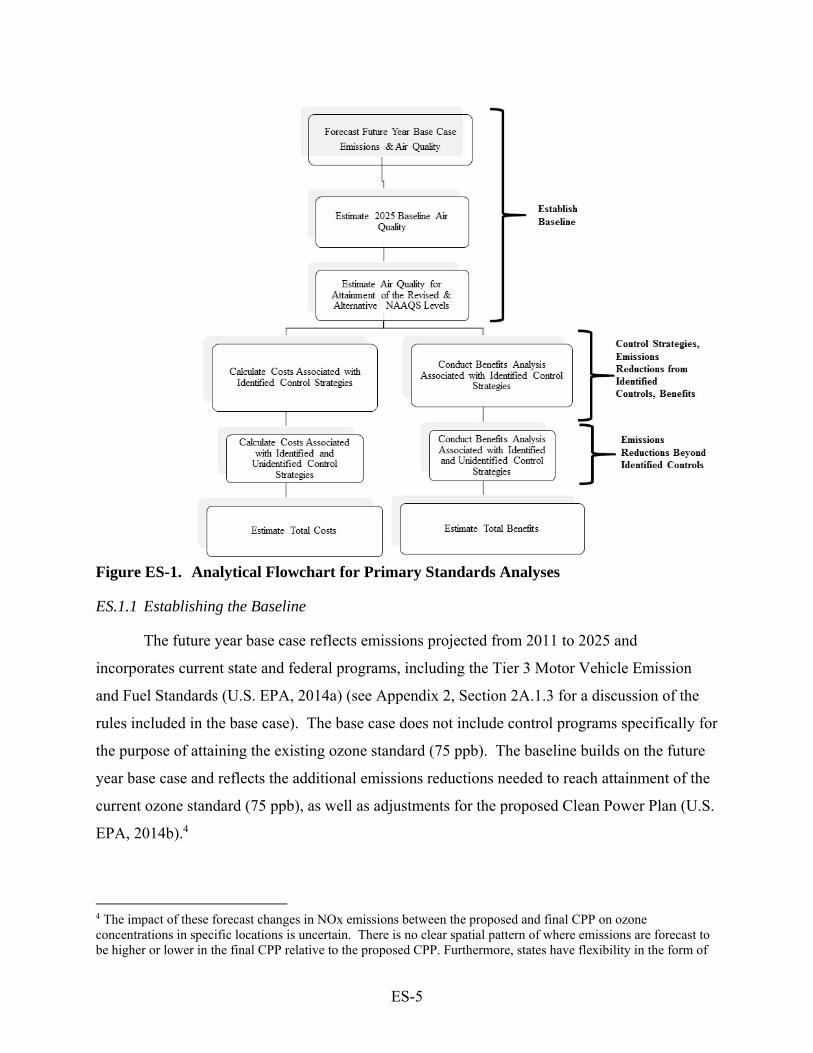
ES-5
Figure ES-1. Analytical Flowchart for Primary Standards Analyses
ES.1.1 Establishing the Baseline
The future year base case reflects emissions projected from 2011 to 2025 and
incorporates current state and federal programs, including the Tier 3 Motor Vehicle Emission
and Fuel Standards (U.S. EPA, 2014a) (see Appendix 2, Section 2A.1.3 for a discussion of the
rules included in the base case). The base case does not include control programs specifically for
the purpose of attaining the existing ozone standard (75 ppb). The baseline builds on the future
year base case and reflects the additional emissions reductions needed to reach attainment of the
current ozone standard (75 ppb), as well as adjustments for the proposed Clean Power Plan (U.S.
EPA, 2014b).4
4 The impact of these forecast changes in NOx emissions between the proposed and final CPP on ozone concentrations in specific locations is uncertain. There is no clear spatial pattern of where emissions are forecast to be higher or lower in the final CPP relative to the proposed CPP. Furthermore, states have flexibility in the form of

ES-6
We performed a national scale air quality modeling analysis to estimate ozone
concentrations for the future base case year of 2025. In addition, we modeled fifteen 2025
emissions sensitivity simulations.5 The emissions sensitivity simulations were used to develop
ozone response factors (ppb/ton) from the modeled response of ozone to changes in NOx and
VOC emissions from various sources and locations. These ozone response factors were then used
to determine the amount of emissions reductions needed to reach the 2025 baseline and to
evaluate the revised and alternative standard levels of 70 and 65 ppb incremental to the
baseline. We used the estimated emissions reductions needed to reach the revised and alternative
standard levels to analyze the costs and benefits.
ES.1.2 Control Strategies and Emissions Reductions
The EPA used the Control Strategy Tool (CoST) to estimate engineering control costs.
We estimated costs for non-electric generating unit point (non-EGU point), nonpoint, and mobile
nonroad sources. Some electric generating units (EGUs) run their control equipment part of the
year. To estimate the costs for EGUs, we assumed they ran their control equipment all year, and
we estimated the costs of additional inputs needed. CoST calculates engineering costs using one
of two different methods: (1) an equation that incorporates key operating unit information, such
as unit design capacity or stack flow rate, or (2) an average annualized cost-per-ton factor
multiplied by the total tons of reduction of a pollutant. The engineering cost analysis uses the
equivalent uniform annual costs (EUAC) method, in which annualized costs are calculated based
on the equipment life for the control measure and the interest rate incorporated into a capital
recovery factor. Annualized costs represent an equal stream of yearly costs over the period the
control technology is expected to operate.
The EPA analyzed illustrative control strategies that areas across the U.S. might employ
to attain the revised primary ozone standard level of 70 ppb and an alternative standard level of
65 ppb. The EPA analyzed the impact that additional emissions control technologies and
their plans that implement the CPP and therefore the specific impact of the CPP on NOx emissions in any state is uncertain. 5 The approach of using emissions sensitivity simulations to determine the response of ozone at monitor locations to emissions changes in specific regions is similar to the approach used in the November 2014 proposal RIA. However, in the final RIA we conducted sensitivity simulations using ten regions compared to five much larger regions in the proposal RIA.
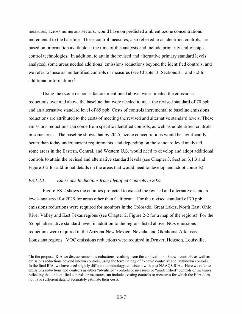
ES-7
measures, across numerous sectors, would have on predicted ambient ozone concentrations
incremental to the baseline. These control measures, also referred to as identified controls, are
based on information available at the time of this analysis and include primarily end-of-pipe
control technologies. In addition, to attain the revised and alternative primary standard levels
analyzed, some areas needed additional emissions reductions beyond the identified controls, and
we refer to these as unidentified controls or measures (see Chapter 3, Sections 3.1 and 3.2 for
additional information).6
Using the ozone response factors mentioned above, we estimated the emissions
reductions over and above the baseline that were needed to meet the revised standard of 70 ppb
and an alternative standard level of 65 ppb. Costs of controls incremental to baseline emissions
reductions are attributed to the costs of meeting the revised and alternative standard levels. These
emissions reductions can come from specific identified controls, as well as unidentified controls
in some areas. The baseline shows that by 2025, ozone concentrations would be significantly
better than today under current requirements, and depending on the standard level analyzed,
some areas in the Eastern, Central, and Western U.S. would need to develop and adopt additional
controls to attain the revised and alternative standard levels (see Chapter 3, Section 3.1.3 and
Figure 3-5 for additional details on the areas that would need to develop and adopt controls).
ES.1.2.1 Emissions Reductions from Identified Controls in 2025
Figure ES-2 shows the counties projected to exceed the revised and alternative standard
levels analyzed for 2025 for areas other than California. For the revised standard of 70 ppb,
emissions reductions were required for monitors in the Colorado, Great Lakes, North East, Ohio
River Valley and East Texas regions (see Chapter 2, Figure 2-2 for a map of the regions). For the
65 ppb alternative standard level, in addition to the regions listed above, NOx emissions
reductions were required in the Arizona-New Mexico, Nevada, and Oklahoma-Arkansas-
Louisiana regions. VOC emissions reductions were required in Denver, Houston, Louisville,
6 In the proposal RIA we discuss emissions reductions resulting from the application of known controls, as well as emissions reductions beyond known controls, using the terminology of “known controls” and “unknown controls.” In the final RIA, we have used slightly different terminology, consistent with past NAAQS RIAs. Here we refer to emissions reductions and controls as either “identified” controls or measures or “unidentified” controls or measures reflecting that unidentified controls or measures can include existing controls or measures for which the EPA does not have sufficient data to accurately estimate their costs.
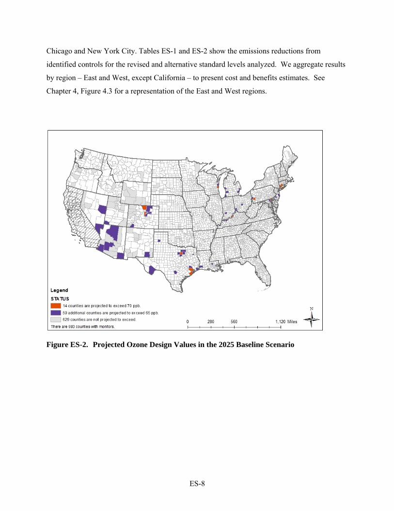
ES-8
Chicago and New York City. Tables ES-1 and ES-2 show the emissions reductions from
identified controls for the revised and alternative standard levels analyzed. We aggregate results
by region – East and West, except California – to present cost and benefits estimates. See
Chapter 4, Figure 4.3 for a representation of the East and West regions.
Figure ES-2. Projected Ozone Design Values in the 2025 Baseline Scenario

ES-9
Table ES-1. Summary of Emissions Reductions by Sector for the Identified Control Strategy for the Revised Standard Level of 70 ppb for 2025, except California (1,000 tons/year)a
Geographic Area Emissions Sector NOx VOC
East
EGU 45 -
Non-EGU Point 85 1
Nonpoint 100 19
Nonroad 3 -
Onroad - -
Total 230 20
West
EGU - -
Non-EGU Point 6 -
Nonpoint 1 -
Nonroad - -
Onroad - -
Total 7 - a Emissions reduction estimates are rounded to two significant figures.
Table ES-2. Summary of Emissions Reductions by Sector for the Identified Control Strategy for Alternative Standard Level of 65 ppb for 2025, except California (1,000 tons/year)a
Geographic Area Emissions Sector NOx VOC
East
EGU 110 -
Non-EGU Point 220 5
Nonpoint 160 100
Nonroad 8 -
Total 500 100
West
EGU 0 -
Non-EGU Point 33 -
Nonpoint 22 5
Nonroad 1 -
Total 56 5 a Emissions reduction estimates are rounded to two significant figures.
ES.1.2.2 Emissions Reductions beyond Identified Controls in 2025
There were several areas where identified controls did not achieve enough emissions
reductions to attain the revised standard level of 70 ppb or alternative standard level of 65 ppb.
The EPA then estimated the additional emissions reductions beyond identified controls needed to
reach attainment (i.e., unidentified controls). The EPA’s application of unidentified control
measures does not mean the Agency has concluded that all unidentified control measures are
currently not commercially available or do not exist. Unidentified control technologies or
measures can include existing controls or measures for which the EPA does not have sufficient
data to accurately estimate engineering costs. Likewise, the control measures in the CoST

ES-10
database do not include abatement possibilities from energy efficiency measures, fuel switching,
input or process changes, or other abatement strategies that are non-traditional in the sense that
they are not the application of an end-of-pipe control. Table ES-3 shows the emissions
reductions needed from unidentified controls in 2025 for the U.S., except California, for the
revised and alternative standard levels analyzed.
Table ES-3. Summary of Emissions Reductions from the Unidentified Control Strategies for the Revised and Alternative Standard Levels for 2025, except California (1,000 tons/year)a
Revised and Alternative Standard
Levels
Region NOx VOC
70 ppb East West
47 -
- -
65 ppb East West
820 40
- -
a Estimates are rounded to two significant figures.
ES.1.2.3 Emissions Reductions beyond Identified Controls for Post-2025
Figure ES-3 shows the counties projected to exceed the revised and alternative standard
levels analyzed for the post-2025 analysis for California. For the California post-2025 revised
and alternative standard level analyses, all identified controls were applied in the baseline, so
incremental emissions reductions to demonstrate attainment of the revised and alternative
standards were from unidentified controls. Table ES-4 shows the emissions reductions needed
from unidentified controls for post-2025 for California for the revised and alternative standard
levels analyzed.
ES-11
Figure ES-3. Projected Ozone Design Values in the Post-2025 Baseline
Table ES-4. Summary of Emissions Reductions from the Unidentified Control Strategies for the Revised and Alternative Standard Levels for Post-2025 - California (1,000 tons/year)a
Revised and Alternative Standard
Levels
Region NOx VOC
70 ppb CA 51 - 65 ppb CA 100 -
a Estimates are rounded to two significant figures.
ES.1.3 Human Health Benefits
To estimate benefits, we follow a “damage-function” approach in calculating total
benefits of the modeled changes in environmental quality. This approach estimates changes in
individual health endpoints (specific effects that can be associated with changes in air quality)
and assigns values to those changes assuming independence of the values for those individual
ES-12
endpoints. Total benefits are calculated as the sum of the values for all non-overlapping health
endpoints. The “damage-function” approach is the standard method for assessing costs and
benefits of environmental quality programs and has been used in several recent published
analyses (Levy et al., 2009; Fann et al., 2012a; Tagaris et al., 2009).
To assess economic values in a damage-function framework, the changes in
environmental quality must be translated into effects on people or on the things that people
value. In some cases, the changes in environmental quality can be directly valued, as is the case
for changes in visibility. In other cases, such as for changes in ozone and PM, an impact analysis
must first be conducted to convert air quality changes into effects that can be later assigned
dollar values. For this RIA, the health impacts analysis is limited to those health effects that are
directly linked to changes in ambient levels of ozone and PM2.5 due to reductions in ozone
precursor emissions. Emissions reductions of NOx or VOC to attain the ozone standards would
simultaneously reduce ambient PM2.5 concentrations.
Benefits estimates for ozone were generated using the damage-function approach outlined
above wherein changes in ambient ozone concentrations were translated into reductions in the
incidence of specific health endpoints (e.g., premature mortality or hospital admissions) using
the environmental Benefits Mapping and Analysis Program – Community Edition (BenMAP-
CE).
In contrast to ozone, we used a benefit-per-ton approach to estimate PM2.5 co-benefits.
With this approach, we use the results of previous air quality modeling to derive benefit-per-ton
estimates for NOx. These benefit-per-ton estimates provide the monetized human health co-
benefits (the sum of premature mortality and premature morbidity) of reducing one ton of a
PM2.5 precursor (such as NOX) from a specified source. We then combine these benefit-per-ton
estimates with reductions in NOx emissions associated with meeting the revised and alternative
standard levels. We acknowledge increased uncertainty associated with the benefit-per-ton
approach, relative to using scenario-specific air quality modeling to estimate the PM2.5 co-
benefits.
In addition to ozone and PM2.5 benefits, implementing emissions controls to attain the
revised and alternative ozone standard levels would reduce exposure to other ambient pollutants

ES-13
(e.g., NO2). However, we were not able to quantify the co-benefits of reduced exposure to these
pollutants, nor were we able to estimate some anticipated health benefits associated with
exposure to ozone and PM2.5 due to data and methodology limitations.
ES.1.4 Welfare Benefits of Meeting the Primary and Secondary Standards
Section 302(h) of the Clean Air Act states that effects on welfare include, but are not
limited to, “effects on soils, water, crops, vegetation, man-made materials, animals, wildlife,
weather, visibility, and climate, damage to and deterioration of property, and hazards to
transportation, as well as effects on economic values and on personal comfort and well-being.”
Ozone can affect ecological systems, leading to changes in the ecological community and
influencing the diversity, health, and vigor of individual species (U.S. EPA, 2013). Ozone causes
discernible injury to a wide array of vegetation (U.S. EPA, 2013). In terms of forest productivity
and ecosystem diversity, ozone may be the pollutant with the greatest potential for region-scale
forest impacts (U.S. EPA, 2013). Studies have demonstrated repeatedly that ozone
concentrations observed in polluted areas can have substantial impacts on plant function (De
Steiguer et al,. 1990; Pye, 1988).
In the RIA for the proposal, we quantified a small portion of the welfare impacts associated
with reductions in ozone concentrations to meet the alternative ozone standard levels analyzed.
Using a model of commercial agriculture and forest markets, we analyzed the effects on
consumers and producers of forest and agricultural products of changes in the W126 index
resulting from meeting alternative standards levels. We also assessed the effects of those
changes in commercial agricultural and forest yields on carbon sequestration and storage. The
analysis provided limited quantitative information on the welfare benefits of meeting alternative
secondary standard levels, focusing only on one subset of ecosystem services. Commercial and
non-commercial forests provide a number of additional services, including medicinal uses, non-
commercial food and fiber production, arts and crafts uses, habitat, recreational uses, and cultural
uses for Native American tribes. In this final RIA, we did not update this analysis and refer to
the analysis conducted in the proposal RIA (U.S. EPA, 2014c). We did not update the analysis
from the proposal RIA because the welfare benefits estimates (i) in the proposal analysis were
small, and we anticipated that the estimates in the final analysis would be even smaller, and (ii)
are not added to the human health benefits estimates.

ES-14
ES.2 Results of Benefit-Cost Analysis
Below in Table ES-5, we present the primary costs and benefits estimates for 2025 for all
areas except California. We anticipate that benefits and costs will likely begin occurring earlier
than 2025, as states begin implementing control measures to show progress towards attainment.
In these tables, ranges within the total benefits rows reflect multiple studies upon which the
estimates associated with premature mortality were derived. PM2.5 co-benefits account for
approximately 60 to 70 percent of the estimated benefits, depending on the standard analyzed
and on the choice of ozone and PM mortality functions used. Assuming a 7 percent discount
rate, for a standard of 70 ppb the total health benefits are comprised of between 29 and 34
percent ozone benefits and between 66 and 71 percent PM2.5 co-benefits. Assuming a 7 percent
discount rate, for a standard of 65 ppb the total health benefits are comprised of between 29 and
35 percent ozone benefits and between 62 and 70 percent PM2.5 co-benefits. In addition for
2025, Table ES-6 presents the numbers of premature deaths avoided for the revised and
alternative standard levels analyzed, as well as the other health effects avoided. Table ES-7
provides information on the costs by geographic region for the U.S., except California in 2025,
and Table ES-8 provides a regional breakdown of benefits for 2025. See the tables in Chapter 6
for additional characterizations of the monetized benefits.
In the RIA we provide estimates of the costs of emissions reductions to attain the revised
and alternative standard levels in three regions -- California, the rest of the western U.S., and the
eastern U.S. In addition, we provide estimates of the benefits that accrue to each of these three
regions resulting from both control strategies applied within the region and reductions in
transport of ozone associated with emissions reductions in other regions.
The net benefits of emissions reductions strategies in a specific region reflect the benefits
of the emissions reductions occurring both within and outside of the region minus the costs of the
emissions reductions. Because the air quality modeling was conducted at the national level, we
do not estimate separately the nationwide benefits associated with the emissions reductions
occurring in any specific region.7 As a result, we are only able to provide net benefits estimates
at the national level. The difference between the costs for a specific region and the benefits
7 For California, we provide separate estimates of the costs and nationwide estimates of benefits, so it is appropriate to calculate net benefits. As such, we provide net benefits for the post-2025 analysis for California.

ES-15
accruing to that region is not an estimate of net benefits of the emissions reductions in that
region.
Table ES-5. Total Annual Costs and Benefitsa,b for U.S., except California in 2025 (billions of 2011$, 7% Discount Rate)c
Revised and Alternative Standard Levels
70 ppb 65 ppb
Total Costsd $1.4 $16 Total Health Benefits $2.9 to $5.9e, f $15 to $30e, f Net Benefits $1.5 to $4.5 -$1.0 to $14
a All values are rounded to two significant figures. b Benefits are nationwide benefits of attainment everywhere except California. c The tables in Chapter 6 provide additional characterizations of the monetized benefits, including benefits estimated at a 3 percent discount rate. Estimating multiple years of costs and benefits is not possible for this RIA due to data and resource limitations. As a result, we provide a snapshot of costs and benefits in 2025, using the best available information to approximate social costs and social benefits recognizing uncertainties and limitations in those estimates.
d The engineering costs in this table are annualized at a 7 percent discount rate to the extent possible. See Chapter 4 for more discussions.
e Assuming a 7 percent discount rate, for a standard of 70 ppb the total health benefits are comprised of between 29 and 34 percent ozone benefits and between 66 and 71 percent PM2.5 co-benefits. Assuming a 7 percent discount rate, for a standard of 65 ppb the total health benefits are comprised of between 29 and 35 percent ozone benefits and between 62 and 70 percent PM2.5 co-benefits.
f Excludes additional health and welfare benefits that could not be quantified (see Chapter 6, Section 6.6.3.8).
The guidelines of OMB Circular A-4 require providing comparisons of social costs and
social benefits at discount rates of 3 and 7 percent. Ideally, streams of social costs and social
benefits over time would be estimated and the net present values of each would be compared to
determine net benefits of the illustrative attainment strategies. The three different uses of
discounting in the RIA – (i) construction of annualized engineering costs, (ii) adjusting the value
of mortality risk for lags in mortality risk decreases, and (iii) adjusting the cost of illness for non-
fatal heart attacks to adjust for lags in follow up costs -- are all appropriate. Our estimates of net
benefits are the approximations of the net value (in 2025) of benefits attributable to emissions
reductions needed to attain just for the year 2025.

ES-16
Table ES-6. Summary of Total Number of Annual Ozone and PM-Related Premature Mortalities and Premature Morbidity: 2025 National Benefits a
Revised and Alternative Standard Levels 70 ppb 65 ppb
Ozone-related premature deaths avoided (all ages) 96 to 160 490 to 820
PM2.5-related premature deaths avoided (age 30+) 220 to 500 1,100 to 2,500
Other health effects avoided
Non-fatal heart attacks (age 18-99) (5 studies) PM 28 to 260
140 to 1,300
Respiratory hospital admissions (age 0-99)O3, PM 250
1,200
Cardiovascular hospital admissions (age 18-99) PM 80
400
Asthma emergency department visits (age 0-99) O3, PM 630
3,300 Acute bronchitis (age 8-12) PM 340 1,700
Asthma exacerbation (age 6-18) O3, PM 230,000 1,100,000
Lost work days (age 18-65) PM 28,000 140,000
Minor restricted activity days (age 18-65) O3, PM 620,000 3,100,000 Upper & lower respiratory symptoms (children 7-14) PM 11,000
53,000
School loss days (age 5-17) O3 160,000 790,000 a Nationwide benefits of attainment everywhere except California. All values are rounded to two significant figures. Additional information on confidence intervals are available in the tables in Chapter 6. Table ES-7. Summary of Total Control Costs (Identified + Unidentified Control
Strategies) by Revised and Alternative Standard Levels for 2025 - U.S., except California (billions of 2011$, 7% Discount Rate)a
Revised and Alternative Standards Levels
Geographic Area
Total Control Costs (Identified and Unidentified)
70 ppb
East 1.4 West <0.05 Total $1.4
65 ppb
East 15 West <0.75 Total $16
a All values are rounded to two significant figures. Costs are annualized at a 7 percent discount rate to the extent possible. Costs associated with unidentified controls are based on an average cost-per-ton methodology (see Chapter 4, Section 4.3 for more discussion on the average-cost methodology).

ES-17
Table ES-8. Regional Breakdown of Monetized Ozone-Specific Benefits Results for 2025 (Nationwide Benefits of Attaining the Revised and Alternative Standard Levels Everywhere in the U.S., except California) a
Revised and Alternative Standard Levels Region 70 ppb 65 ppb East b 98% 96%
California 0% 0% Rest of West 2% 4%
a Because we use benefit-per-ton estimates to calculate the PM2.5 co-benefits, a regional breakdown for the co-benefits is not available. Therefore, this table only reflects the ozone benefits. b Includes Texas and states to the north and east.
To understand possible additional costs and benefits of fully attaining in California in a
post-2025 timeframe, we provide separate results for California in Table ES-9. Because of the
differences in the timing of achieving needed emissions reductions, incurring costs, and accruing
benefits for California, the separate costs and benefits estimates for post-2025 should not be
added to the primary estimates for 2025. For the post-2025 timeframe, Table ES-10 presents the
numbers of premature deaths avoided for the revised and alternative standard levels analyzed, as
well as the other health effects avoided. Table ES-11 provides information on the costs for
California for post-2025, and Table ES-12 provides a regional breakdown of benefits for post-
2025.
The EPA presents separate costs and benefits results for California because assuming
attainment in an earlier year than would be required under the Clean Air Act would likely lead to
an overstatement of costs and benefits because California might benefit from some existing
federal or state programs that would be implemented between 2025 and the ultimate attainment
years; because additional new technologies may become available between 2025 and the
attainment years; and because the cost of existing technologies might fall over time. As such, we
use the best available data to estimate costs and benefits for California in a post-2025 timeframe,
but because of data limitations and additional uncertainty associated with not projecting
emissions and air quality beyond 2025, we recognize that the estimates of costs and benefits for
California in a post-2025 timeframe are likely to be relatively more uncertain than the national
attainment estimates for 2025.
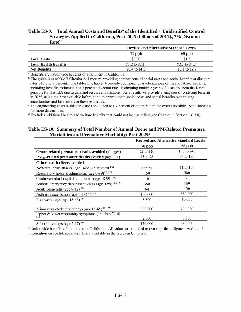
ES-18
Table ES-9. Total Annual Costs and Benefitsa of the Identified + Unidentified Control Strategies Applied in California, Post-2025 (billions of 2011$, 7% Discount Rate)b
Revised and Alternative Standard Levels
70 ppb 65 ppb
Total Costsc $0.80 $1.5 Total Health Benefits $1.2 to $2.1d $2.3 to $4.2d Net Benefits $0.4 to $1.3 $0.8 to $2.7
a Benefits are nationwide benefits of attainment in California. b The guidelines of OMB Circular A-4 require providing comparisons of social costs and social benefits at discount rates of 3 and 7 percent. The tables in Chapter 6 provide additional characterizations of the monetized benefits, including benefits estimated at a 3 percent discount rate. Estimating multiple years of costs and benefits is not possible for this RIA due to data and resource limitations. As a result, we provide a snapshot of costs and benefits in 2025, using the best available information to approximate social costs and social benefits recognizing uncertainties and limitations in those estimates.
c The engineering costs in this table are annualized at a 7 percent discount rate to the extent possible. See Chapter 4 for more discussions.
d Excludes additional health and welfare benefits that could not be quantified (see Chapter 6, Section 6.6.3.8). Table ES-10. Summary of Total Number of Annual Ozone and PM-Related Premature
Mortalities and Premature Morbidity: Post-2025a Revised and Alternative Standard Levels
70 ppb 65 ppb
Ozone-related premature deaths avoided (all ages) 72 to 120 150 to 240
PM2.5-related premature deaths avoided (age 30+) 43 to 98 84 to 190
Other health effects avoided
Non-fatal heart attacks (age 18-99) (5 studies) PM 6 to 51 11 to 100
Respiratory hospital admissions (age 0-99)O3, PM 150 300
Cardiovascular hospital admissions (age 18-99) PM 16 31
Asthma emergency department visits (age 0-99) O3, PM 380 760
Acute bronchitis (age 8-12) PM 64 130
Asthma exacerbation (age 6-18) O3, PM 160,000 330,000
Lost work days (age 18-65) PM 5,300 10,000
Minor restricted activity days (age 18-65) O3, PM 360,000
720,000 Upper & lower respiratory symptoms (children 7-14) PM 2,000
3,900
School loss days (age 5-17) O3 120,000 240,000 a Nationwide benefits of attainment in California. All values are rounded to two significant figures. Additional information on confidence intervals are available in the tables in Chapter 6.

ES-19
Table ES-11. Summary of Total Control Costs (Identified + Unidentified Control Strategies) by Revised and Alternative Standards for Post-2025 - California (billions of 2011$, 7% Discount Rate)a
Revised and Alternative Standard Level
Geographic Area Total Control Costs
(Identified and Unidentified)
70 ppb California $0.80 65 ppb California $1.5
a All values are rounded to two significant figures. Costs are annualized at a 7 percent discount rate to the extent possible. Costs associated with unidentified controls are based on an average cost-per-ton methodology.
Table ES-12. Regional Breakdown of Monetized Ozone-Specific Benefits Results for Post-2025 (Nationwide Benefits of Attaining Revised and Alternative Standards just in California)a
Revised and Alternative Standard Levels Region 70 ppb 65 ppb East b 3% 2%
California 90% 91% Rest of West 7% 7%
a Because we use benefit-per-ton estimates to calculate the PM2.5 co-benefits, a regional breakdown for the co-benefits is not available. Therefore, this table only reflects the ozone benefits. b Includes Texas and states to the north and east. ES.3 Improvements between the Proposal and Final RIAs
In the regulatory impact analyses for both the proposed and final ozone NAAQS, there
were two geographic areas outside of California where the majority of emissions reductions were
needed to meet the revised standard level of 70 ppb – Texas and the Northeast. In analyzing 70
ppb in the final RIA, there were approximately 50 percent fewer emissions reductions needed in
these two geographic areas. For an alternative standard of 65 ppb in the final RIA, emissions
reductions needed nationwide were approximately 20 percent lower than at proposal. The
primary reason for the difference in emissions reductions estimated for attainment is that in the
final RIA we conducted more geographically-refined air quality sensitivity modeling to develop
improved ozone response factors (see Chapter 2, Section 2.2.2 for a more detailed discussion of
the air quality modeling) and focused the emissions reduction strategies on geographic areas
closer to the monitors with the highest design values (see Chapter 3, Section 3.1.1 for a more
detailed discussion of the emissions reduction strategies). The improvements in air quality
modeling and emissions reduction strategies account for about 80 percent of the difference in
needed emissions reductions between the proposal and final RIAs.
ES-20
In Texas and the Northeast, the updated response factors and more focused emissions
reduction strategies resulted in larger changes in ozone concentrations in response to more
geographically focused emissions reductions. In east Texas, the ppb/ton ozone response factors
used in the final RIA were 2 to 3 times more responsive than the factors used in the proposal
RIA at controlling monitors in Houston and Dallas. In the Northeast, the ppb/ton ozone response
factors used in the final RIA were 2.5 times more responsive than the factors used in the proposal
RIA at the controlling monitor on Long Island, NY.
A secondary reason for the difference is that between the proposal and final RIAs we
updated emissions inventories, models and model inputs for the base year of 2011. See
Appendix 2, Section 2A.1.3 for additional discussion of the updated emissions inventories,
models and model inputs. When projected to 2025, these changes in inventories, models and
inputs had compounding effects for year 2025, and in some areas resulted in lower projected
base case design values for 2025. The updated emissions inventories, models, and model inputs
account for about 20 percent of the difference in needed emissions reductions between the
proposal and final RIAs.
These differences in the estimates of emissions reductions needed to attain the revised
and alternative standard levels affect the estimates for the costs and benefits in this RIA. For a
revised standard of 70 ppb, the costs were 60 percent lower than at proposal and the benefits
were 55 percent lower than at proposal. The percent decrease in costs is slightly more than the
percent decrease in emissions reductions because a larger number of lower cost identified
controls were available to bring areas into attainment with 70 ppb.8 The percent decrease in
benefits is similar to the percent decrease in emissions reductions. For an alternative standard
level of 65 ppb, the costs were less than three percent more than those estimated at proposal and
the benefits were 22 percent lower than at proposal. The percent change in costs was less than
the percent decrease in emissions reductions because in the final analysis we applied identified
controls in smaller geographic areas, resulting in fewer identified controls available within those
8 In the final RIA, outside of California all areas were projected to meet the current standard of 75 ppb. As such, no identified controls were used to bring areas into attainment with 75 ppb. In the proposal RIA, some of these lower cost controls were used to bring areas into attainment with 75 ppb, making them unavailable for application in the analysis of 70 ppb.
ES-21
areas and an increase in higher cost unidentified controls being applied to bring areas into
attainment with 65 ppb. The percent decrease in benefits is similar to the percent decrease in
emissions reductions.
ES.4 Uncertainty
Despite uncertainties inherent in any complex, quantitative analysis, the underlying tools
and models (CoST and BenMAP) have been peer-reviewed and the analytical methods are
consistent with standard economic practice. For a detailed discussion on uncertainty associated
with developing illustrative control strategies to attain the alternative standard levels, see Chapter
3, Section 3.4. For a description of the key assumptions and uncertainties related to ozone
benefits, see Chapter 6, Section 6.5, and for an additional qualitative discussion of sources of
uncertainty associated with both ozone-related benefits and PM2.5-related co-benefits, see
Appendix 6A. For a discussion of the limitations and uncertainties in the engineering cost
analyses, see Chapter 4, Section 4.7. For a general discussion about key factors that could
impact how air quality changes over time, see Chapter 8, Section 8.3.
ES.5 References
De Steiguer, J., Pye, J., Love, C. 1990. Air Pollution Damage to U.S. Forests. Journal of Forestry, 88(8), 17-22.
Fann N, Lamson A, Wesson K, Risley D, Anenberg SC, Hubbell BJ. 2012a. “Estimating the National Public Health Burden Associated with Exposure to Ambient PM2.5 and ozone. Risk Analysis,” Risk Analysis 32(1): 81-95.
Levy JI, Baxter LK, Schwartz J. 2009. “Uncertainty and variability in health-related damages from coal-fired power plants in the United States.” Risk Analysis 29(7) 1000-1014.
Pye, J.M. 1988. Impact of ozone on the growth and yield of trees: A review. Journal of Environmental Quality, 17, 347-360.
Tagaris E, Liao KJ, Delucia AJ, et al. 2009. “Potential impact of climate change on air-pollution related human health effects.” Environmental Science & Technolology 43: 4979–4988.
U.S. Environmental Protection Agency (U.S. EPA). 2013. Integrated Science Assessment of Ozone and Related Photochemical Oxidants (Final Report). EPA-600/R-10/076F. February. Available at <http://cfpub.epa.gov/ncea/isa/recordisplay.cfm?deid=247492>.
U.S. Environmental Protection Agency (U.S. EPA). 2014a. Control of Air Pollution from Motor Vehicles: Tier 3 Motor Vehicle Emission and Fuel Standards. Office of Transportation and Air Quality. Available at <http://www.epa.gov/otaq/tier3.htm>.
U.S. Environmental Protection Agency (U.S. EPA). 2014b. Proposed Carbon Pollution Guidelines for Existing Power Plants and Emission Standards for Modified and Reconstructed Power Plants. Available at <http://www2.epa.gov/sites/production/files/2014-06/documents/20140602ria-clean-power-plan.pdf>.

ES-22
U.S. Environmental Protection Agency (U.S. EPA). 2014c. Regulatory Impact Analysis of the Proposed Revisions to the National Ambient Air Quality Standards for Ground-Level Ozone. Office of Air Quality Planning and Standards, Research Triangle Park, NC. November. Available at <http://www.epa.gov/ttnecas1/regdata/RIAs/20141125ria.pdf >.
1-1
CHAPTER 1: INTRODUCTION AND BACKGROUND
Introduction
The Environmental Protection Agency (EPA) initiated the current ozone National
Ambient Air Quality Standards (NAAQS) review in September 2008. Between 2008 and 2014,
the EPA prepared draft and final versions of the Integrated Science Assessment, the Health and
Welfare Risk and Exposure Assessments, and the Policy Assessment. Multiple drafts of these
documents were available for public review and comment. In addition, as required by the Clean
Air Act (CAA), the documents were peer-reviewed by the Clean Air Scientific Advisory
Committee (CASAC), the Administrator’s independent advisory committee established by the
CAA. The final documents for this review reflect the EPA staff’s consideration of the comments
and recommendations made by the CASAC and the public on draft versions of these documents.
The EPA has concluded that the current primary standard for ozone, set at a level of 75
ppb, is not requisite to protect public health with an adequate margin of safety, and is revising
the standard to provide increased public health protection. Specifically, the EPA is retaining the
indicator (ozone), averaging time (8-hour) and form (annual fourth-highest daily maximum,
averaged over 3 years) of the existing primary standard and is revising the level of that standard
to 70 ppb. The EPA is making this revision to increase public health protection, including for
“at-risk” populations such as children, older adults, and people with asthma or other lung
diseases, against an array of ozone-related adverse health effects. For short-term ozone
exposures, these effects include decreased lung function, increased respiratory symptoms and
pulmonary inflammation, effects that result in serious indicators of respiratory morbidity such as
emergency department visits and hospital admissions, and all-cause (total non-accidental)
mortality. For long-term ozone exposures, these health effects include a variety of respiratory
morbidity effects and respiratory mortality.
The EPA has also concluded that the current secondary standard for ozone, set at a level
of 75 ppb, is not requisite to protect public welfare from known or anticipated adverse effects,
and is revising the standard to provide increased protection against vegetation-related effects on
public welfare. Specifically, the EPA is retaining the indicator (ozone), averaging time (8-hour)
1-2
and form (annual fourth-highest daily maximum, averaged over 3 years) of the existing
secondary standard and is revising the level of that standard to 70 ppb. The EPA has concluded
that this revision will effectively curtail cumulative seasonal ozone exposures above 17 ppm-hrs,
in terms of a three-year average seasonal W126 index value, based on the three consecutive
month period within the growing season with the maximum index value, with daily exposures
cumulated for the 12-hour period from 8:00 am to 8:00 pm. Thus, the EPA has concluded that
this revision will provide the requisite protection against known or anticipated adverse effects to
the public welfare.
This Regulatory Impact Analysis (RIA) analyzes the human health benefits and costs and
welfare cobenefits of the revised standard of 70 ppb as well as a more stringent alternative level
of 65 ppb. In setting primary ambient air quality standards, the EPA’s responsibility under the
law is to establish standards that protect public health, regardless of the costs of implementing
those standards. As interpreted by the Agency and the courts, the CAA requires the EPA to
create standards based on health considerations only.
The prohibition against the consideration of cost in the setting of the primary air quality
standards, however, does not mean that costs or other economic considerations are unimportant
or should be ignored. The Agency believes that consideration of costs and benefits is essential to
making efficient, cost-effective decisions for implementing these standards. The impact of cost
and efficiency is considered by states during the implementation process, as they decide what
timelines, strategies, and policies are appropriate for their circumstances. This RIA is intended to
inform the public about the potential costs and benefits that may result when new standards are
implemented, but it is not part of setting the standards.
This chapter summarizes provides a brief background on NAAQS, the need for NAAQS,
and an overview of this RIA, including a discussion of its design. The EPA prepared this RIA
both to provide the public with information on the benefits and costs of meeting a revised ozone
NAAQS and to meet the requirements of Executive Orders 12866 and 13563.

1-3
1.1 Background
1.1.1 National Ambient Air Quality Standards
Sections 108 and 109 of the CAA govern the establishment and revision of the NAAQS.
Section 108 (42 U.S.C. 7408) directs the Administrator to identify pollutants that “may
reasonably be anticipated to endanger public health or welfare” and to issue air quality criteria
for them. These air quality criteria are intended to “accurately reflect the latest scientific
knowledge useful in indicating the kind and extent of all identifiable effects on public health or
welfare which may be expected from the presence of [a] pollutant in the ambient air.” Ozone is
one of six pollutants for which the EPA has developed air quality criteria.
Section 109 (42 U.S.C. 7409) directs the Administrator to propose and promulgate
“primary” and “secondary” NAAQS for pollutants identified under section 108. Section
109(b)(1) defines a primary standard as an ambient air quality standard “the attainment and
maintenance of which in the judgment of the Administrator, based on [the] criteria and allowing
an adequate margin of safety, [is] requisite to protect the public health.” A secondary standard, as
defined in section 109(b)(2), must “specify a level of air quality the attainment and maintenance
of which in the judgment of the Administrator, based on [the] criteria, is requisite to protect the
public welfare from any known or anticipated adverse effects associated with the presence of
[the] pollutant in the ambient air.” Welfare effects as defined in section 302(h) [42 U.S.C.
7602(h)] include but are not limited to “effects on soils, water, crops, vegetation, manmade
materials, animals, wildlife, weather, visibility and climate, damage to and deterioration of
property, and hazards to transportation, as well as effects on economic values and on personal
comfort and well-being.”
Section 109(d) of the CAA directs the Administrator to review existing criteria and
standards at 5-year intervals. When warranted by such review, the Administrator is to retain or
revise the NAAQS. After promulgation or revision of the NAAQS, the standards are
implemented by the states.
1.1.2 Role of Executive Orders in the Regulatory Impact Analysis
While this RIA is separate from the NAAQS decision-making process, several statutes and
executive orders still apply to any public documentation. The analyses required by these statutes

1-4
and executive orders are presented in detail in Chapter 9, and below we briefly discuss
requirements of Orders 12866 and 13563 and the guidelines of the Office of Management and
Budget (OMB) Circular A-4 (U.S. OMB, 2003).
In accordance with Executive Orders 12866 and 13563 and the guidelines of OMB
Circular A-4, the RIA analyzes the benefits and costs associated with emissions controls to attain
the revised 8-hour ozone standard of 70 ppb in ambient air, incremental to a baseline of attaining
the existing standard (8-hour ozone standard of 75 ppb).9 OMB Circular A-4 requires analysis of
one potential alternative standard level more stringent than the revised standard and one less
stringent than the revised standard. In this RIA, we analyze a more stringent alternative standard
level of 65 ppb. The existing standard of 75 ppb represents the less stringent alternative standard
and the costs and benefits of this standard were presented in the 2008 ozone NAAQS RIA (U.S.
EPA, 2008a). Further, as discussed in the notice of final rulemaking, the available scientific
evidence and quantitative risk and exposure information on the health effects of ozone exposure
provide strong support for a revised standard of 70 ppb, but do not identify a bright line for
identifying any specific standard level between 70 and 75 ppb for analysis in the RIA. As such,
we did not analyze a standard between 70 and 75 ppb in this RIA.
1.1.3 Illustrative Nature of the Analysis
The control strategies presented in this RIA are an illustration of one possible set of control
strategies states might choose to implement to meet the revised standards. States—not the
EPA—will implement the revised NAAQS and will ultimately determine appropriate emissions
control strategies and measures. State Implementation Plans (SIPs) will likely vary from the
EPA’s estimates provided in this analysis due to differences in the data and assumptions that
states use to develop these plans. Because states are ultimately responsible for implementing
strategies to meet the revised standards, the control strategies in this RIA are considered
hypothetical. The hypothetical strategies were constructed with the understanding that there are
9 On April 30, 2012 the EPA issued final designations for the 2008 ozone NAAQS. After final designations, areas have up to three years to submit attainment SIPs. Because of the timing of these SIP submittals, the EPA does not have the most current information on control measures and emissions reductions needed to meet the current standard of 75 ppb. To account for potential emissions reductions associated with meeting the current standard, we estimate these emissions reductions in defining the baseline.

1-5
inherent uncertainties in projecting emissions and control applications. Additional important
uncertainties and limitations are documented in the relevant portions of the RIA.
The EPA’s national program rules require technology application or emissions limits for a
specific set of sources or source groups. In contrast, a NAAQS establishes a standard level and
requires states to identify and secure emissions reductions to meet the standard level from any set
of sources or source groups. To avoid double counting the impacts of NAAQS and other
national program rules, the EPA includes federal regulations and enforcement actions in its
baseline for this analysis (See Section 1.3.1 for additional discussion of the baseline). The
benefits and costs of the revised standards will not be realized until specific control measures are
mandated by SIPs or other federal regulations.
1.2 The Need for National Ambient Air Quality Standards
OMB Circular A-4 indicates that one of the reasons a regulation such as the NAAQS may
be issued is to address a market failure. The major types of market failure include: externality,
market power, and inadequate or asymmetric information. Correcting market failures is one
reason for regulation, but it is not the only reason. Other possible justifications include
improving the function of government, removing distributional unfairness, or promoting privacy
and personal freedom.
Environmental problems are classic examples of externalities -- uncompensated benefits or
costs imposed on another party as a results of one’s actions. For example, the smoke from a
factory may adversely affect the health of local residents and soil the property in nearby
neighborhoods. If bargaining was costless and all property rights were well defined, people
would eliminate externalities through bargaining without the need for government regulation.
From an economics perspective, setting an air quality standard is a straightforward remedy
to address an externality in which firms emit pollutants, resulting in health and environmental
problems without compensation for those incurring the problems. Setting a standard with a
reasonable margin of safety attempts to place the cost of control on those who emit the pollutants
and lessens the impact on those who suffer the health and environmental problems from higher
levels of pollution. For additional discussion on the ozone air quality problem, see Chapter 2 of

1-6
the Policy Assessment for the Review of the Ozone National Ambient Air Quality Standards (US
EPA, 2014).
1.3 Overview and Design of the RIA
The RIA evaluates the costs and benefits of hypothetical national control strategies to
attain the revised ozone standard of 70 ppb and an alternative ozone standard level of 65 ppb.
1.3.1 Establishing Attainment with the Current Ozone National Ambient Air Quality Standard
The RIA is intended to evaluate the overall potential costs and benefits of reaching
attainment with the revised and alternative ozone standard levels. To develop and evaluate
control strategies for attaining a more stringent primary standard, it is important to estimate
ozone levels in the future after attaining the current NAAQS of 75 ppb, and taking into account
projections of future air quality reflecting on-the-books Federal regulations, substantial federal
regulatory proposals, enforcement actions, state regulations, population and where possible,
economic growth. Establishing this baseline for the analysis then allows us to estimate the
incremental costs and benefits of attaining the revised and alternative standard levels.
Attaining 75 ppb reflects emissions reductions (i) already achieved as a result of national
regulations, (ii) expected prior to 2025 from recently promulgated national regulations (i.e.,
reductions that were not realized before promulgation of the previous standard, but are expected
prior to attainment of the current ozone standard), and (iii) from additional controls that the EPA
estimates need to be included to attain the current standard. Additional emissions reductions
achieved as a result of state and local agency regulations and voluntary programs are reflected to
the extent that they are represented in emissions inventory information submitted to the EPA by
state and local agencies. We took two steps to develop the baseline for this analysis, a baseline
that reflects attainment of 75 ppb. First, national ozone concentrations were projected to the
analysis year (2025) based on forecasts of population and where possible, economic growth and
the application of emissions controls resulting from national rules promulgated prior to this
analysis, as well as state programs and enforcement actions. Second, we estimated additional
emissions reductions needed to meet the current standard of 75 ppb and make adjustments for the
proposed Clean Power Plan.
1-7
Below is a list of some of the national rules reflected in the baseline. For a more complete
list, please see the Technical Support Document: Preparation of Emissions Inventories for the
Version 6.2, 2011 Emissions Modeling Platform (US EPA, 2015). If the national rules reflected
in the baseline result in changes in ozone concentrations or actual emissions reductions that are
lower or higher than those estimated, the costs and benefits estimated in this final RIA would be
higher or lower, respectively.
Carbon Pollution Emission Guidelines for Existing Stationary Sources: Electric Utility Generating Units (Proposed Rule) (U.S. EPA, 2014a)
Tier 3 Motor Vehicle Emission and Fuel Standards (U.S. EPA, 2014c)
2017 and Later Model Year Light-Duty Vehicle Greenhouse Gas Emissions and Corporate Average Fuel Economy Standards (U.S. EPA, 2012)
Cross State Air Pollution Rule (CSAPR) (U.S. EPA, 2011)
Mercury and Air Toxics Standards (U.S. EPA, 2011a)10
Greenhouse Gas Emissions Standards and Fuel Efficiency Standards for Medium- and Heavy-Duty Engines and Vehicles (U.S. EPA, 2011d)11
C3 Oceangoing Vessels (U.S. EPA, 2010)
Reciprocating Internal Combustion Engines (RICE) NESHAPs (U.S. EPA, 2010a)
Regulation of Fuels and Fuel Additives: Modifications to Renewable Fuel Standard Program (RFS2) (U.S. EPA, 2010b)
Light-Duty Vehicle Greenhouse Gas Emission Standards and Corporate Average Fuel Economy Standards; Final Rule for Model-Year 2012-2016 (U.S. EPA, 2010c)
Hospital/Medical/Infectious Waste Incinerators: New Source Performance Standards and Emission Guidelines: Final Rule Amendments (U.S. EPA, 2009)
10 On June 29, 2015, the United States Supreme Court reversed the D.C. Circuit opinion affirming the Mercury and Air Toxics Standards (MATS). The EPA is reviewing the decision and will determine any appropriate next steps once the review is complete, however, MATS is still currently in effect. The first compliance date was April 2015, and many facilities have installed controls for compliance with MATS. MATS is included in the baseline for this analysis, and the EPA does not believe including MATS substantially alters the results of this analysis. 11 This rule is Phase 1 of the Heavy Duty Greenhouse Gas Standards for New Vehicles and Engines (76 FR 57106, September 15, 2011) and is included in the 2025 base case. Phase 2 of the Heavy Duty Greenhouse Gas Standards for New Vehicles and Engines (80 FR 40138, July 13, 2015) is not included in the 2025 base case because the rulemaking was not finalized in time to include in this analysis. If the emissions reductions from Phase 1 were not included in the baseline in this analysis, the estimated costs and benefits of achieving the revised and alternative standards analyzed would be higher because more emissions reductions would be needed.

1-8
Emissions Standards for Locomotives and Marine Compression-Ignition Engines (U.S. EPA, 2008b)
Control of Emissions for Nonroad Spark Ignition Engines and Equipment (U.S. EPA, 2008c)
Regional Haze Regulations and Guidelines for Best Available Retrofit Technology Determinations (U.S. EPA, 2005a)
NOx Emission Standard for New Commercial Aircraft Engines (U.S. EPA, 2005)
To define the baseline in the ozone NAAQS final RIA, we adjusted the 2025 final ozone
NAAQS base case air quality to reflect the proposed Clean Power Plan (CPP) using the Option 1
State illustrative compliance approach from the CPP proposal RIA. We recognize that the
difference in forecast NOx emissions from the electricity sector between the CPP proposal and
final likely has some effect on baseline ozone concentrations, and therefore on estimated NOx
emissions reductions needed to meet the ozone standards analyzed in the NAAQS final RIA.
The power sector modeling for the final CPP reflected updated inputs including lower
costs for new renewable energy resources and changes in the composition of electric generating
resources relative to the baseline used for the proposed CPP. These updated inputs resulted in
changes in the baseline level and spatial distribution of NOx emissions in the final CPP. In
addition, in the final CPP the CO2 emissions goals for states and compliance timing changed
from the proposal, which further changed the level and spatial distribution of NOx emissions.
The net effect of these changes is that total forecast annual NOx emissions in 2025 for the
electricity sector were between 13,000 and 51,000 tons lower under the final CPP than under the
proposed CPP.
The impact of these forecast changes in NOx emissions on ozone concentrations in specific
locations is uncertain. There is no clear spatial pattern of where emissions are forecast to be
higher or lower in the final CPP relative to the proposed CPP. Furthermore, states have
flexibility in the form of their plans that implement the CPP and therefore the specific impact of
the CPP on NOx emissions in any state is uncertain. Finally, because no air quality modeling was
done for the final CPP, we are not able to implement the same approach to reflect the impact of

1-9
the final CPP on ozone air quality in the NAAQS baseline that we used to account for the
proposed CPP in the baseline.
We recognize that not accounting for the final CPP in the baseline introduces additional
uncertainty into the NAAQS final RIA. However, in the final CPP EPA recommends that states
take a multipollutant planning approach that recognizes co-pollutant impacts of CO2 compliance
decisions and takes into account local air quality impacts. Given the flexibility that states have
in addressing both their CO2 and air quality requirements, EPA expects that states will design
strategies to meet both the CPP and NAAQS in the most cost-effective manner12, and thus costs
for the combined set of actions will likely differ from the combined costs provided in the
separate RIAs.
The baseline for this analysis does not assume emissions controls that might be
implemented to meet the current PM2.5, NO2, or SO2 NAAQS. For the current PM2.5 and SO2
NAAQS, the Agency has not issued final designations and does not have information on what
areas would need emissions controls; for the current NO2 NAAQS there are no nonattainment
areas. We did not conduct this analysis incremental to controls applied as part of previous
NAAQS analyses because the data and modeling on which these previous analyses were based
are now considered outdated and are not compatible with the current ozone NAAQS analysis.13
More importantly, all control strategies analyzed in NAAQS RIAs are hypothetical.
12 “…the EPA believes that the Clean Power Plan provides an opportunity for states to consider strategies for
meeting future CAA planning obligations as they develop their plans under this rulemaking. Multi-pollutant strategies that incorporate criteria pollutant reductions over the planning horizons specific to particular states, jointly with strategies for reducing CO2 emissions from affected EGUs needed to meet Clean Power Plan requirements over the time horizon of this rule, may accomplish greater environmental results with lower long-term costs.” Page 1333 of the Carbon Pollution Emission Guidelines for Existing Stationary Sources: Electric Utility Generating Units, currently available at the following link: http://www2.epa.gov/sites/production/files/2015-08/documents/cpp-final-rule.pdf. In the future, please refer to the official version in a forthcoming FR publication, which will appear on the Government Printing Office's FDSys website
(http://gpo.gov/fdsys/search/home.action) and on Regulations.gov (http://www.regulations.gov) in Docket No. EPA–HQ–OAR–2013-0602.
13 There were no additional NOx controls applied in the 2012 PM2.5 NAAQS RIA, and therefore there would be little to no impact on the controls selected in this analysis. In addition, the only geographic areas that exceed the alternative ozone standard levels analyzed in this RIA and in the 2012 PM2.5 NAAQS RIA are in California. The attainment dates for a new PM2.5 NAAQS would likely precede attainment dates for a revised ozone NAAQS. While the 2012 PM2.5 NAAQS RIA concluded that controls on directly emitted PM2.5 were the most cost-effective controls on a $/ug basis, states may choose to adopt different control options. These options could
1-10
1.3.2 Establishing the Baseline for Evaluation of Revised and Alternative Standards
The RIA evaluates, to the extent possible, the costs and benefits of attaining the revised
and alternative ozone standards incremental to attaining the current ozone standard and
implementing existing and expected regulations. We assume that potential nonattainment areas
everywhere in the U.S., excluding California, will be designated such that they are required to
attain the revised standard by 2025. As such, we developed our projected baselines for
emissions, air quality, and populations and present the primary costs and benefits estimates for
2025.
The selection of 2025 as the analysis year in the RIA does not predict or prejudge
attainment dates that will ultimately be assigned to individual areas under the CAA. The CAA
contains a variety of potential attainment dates and flexibility to move to later dates (up to 20
years), provided that the date is as expeditious as practicable. The EPA will likely finalize
designations for a revised ozone NAAQS in late 2017. Depending on the precise timing of the
effective date of those designations, nonattainment areas classified as Marginal will likely have
to attain in either late 2020 or early 2021. Nonattainment areas classified as Moderate will likely
have to attain in either late 2023 or early 2024. If a Moderate nonattainment area qualifies for
two 1-year extensions, the area may have as late as early 2026 to attain. Lastly, Serious
nonattainment areas will likely have to attain in late 2026 or early 2027. We selected 2025 as the
primary year of analysis because it provides a good representation of the remaining air quality
concerns that Moderate nonattainment areas would face and because most areas of the U.S. will
likely be required to meet a revised ozone standard by 2025. States with areas classified as
Moderate and higher are required to develop attainment demonstration plans for those
nonattainment areas.
The EPA recognizes that areas designated nonattainment for the revised ozone NAAQS
and classified as Marginal or Moderate will likely incur some costs prior to the 2025 analysis
year. The Agency, however, anticipates that on-the-books federal emissions control measures14
will be sufficient to bring the majority of these areas into attainment by 2025. Areas designated
include NOx controls, and it is difficult to determine the impact on costs and benefits for this RIA because it depends highly on the control measures that would be chosen and the costs of these measures.
14 These federal control measures are listed above in section 1.3.1.
1-11
nonattainment and classified as Marginal are required to develop emission inventories, emission
statements, and produce a CAA section 110 infrastructure SIP. These areas are not required to
develop any control measures aside from the federal emissions control measures reflected in the
baseline. As a result, the Agency anticipates that costs in these Marginal areas will be minimal.
In addition to the federal control measures and the requirements for Marginal nonattainment
areas, states with nonattainment areas designated as Moderate are required by the CAA to
develop state implementation plans (SIPs) demonstrating attainment by no later than the assigned
attainment date. The CAA also requires these states to address Reasonably Available Control
Technologies (RACT) for sources in the Moderate nonattainment area, which could lead to
additional point source controls in an area beyond the federal emissions control measures.
Additionally, the CAA requires some Moderate areas with larger populations to implement basic
vehicle inspection and maintenance (I/M) in the area. Should these federal programs and CAA
required programs prove inadequate for the area to attain the revised standard by the attainment
date, the state would need to identify additional emissions control measures in its SIP to meet
attainment requirements.
In addition, in estimating the incremental costs and benefits of the revised and alternative
standards, we recognize that there are areas that are not required to meet the existing ozone
standard by 2025 -- the CAA allows areas with more significant air quality problems to take
additional time to reach the existing standard. Several areas in California are not required to
meet the existing standard by 2025 and may not be required to meet a revised standard until
sometime between 2032 and 2037.15,16 Because of data and resource constraints, we were not
able to project emissions and air quality beyond 2025 for California, however, we adjusted
baseline air quality to reflect mobile source emissions reductions for California that would occur
between 2025 and 2030; these emissions reductions were the result of mobile source regulations
15 The EPA will likely finalize designations for a revised ozone NAAQS in late 2017. Depending on the precise timing of the effective date of those designations, nonattainment areas classified as Severe 15 will likely have to attain by December 31, 2032 and nonattainment areas classified as Extreme will likely have to attain by December 31, 2037. 16 In this RIA before deciding to continue to analyze California beyond the future analysis year of 2025, we reviewed California’s NOx and VOC emissions within existing nonattainment areas. The vast majority of these emissions come from emissions sources located in existing nonattainment areas that would likely have to attain the final standard sometime between 2032 and 2037. As a result, we concluded that analyzing California separately and after 2025 continued to be an appropriate analytical decision.

1-12
expected to be fully implemented by 2030.17 While there is uncertainty about the precise timing
of emissions reductions and related costs for California, we assume costs occur through the end
of 2037 and beginning of 2038. In addition, we model benefits for California using projected
population demographics for 2038.
Because of the difference in timing for incurring costs and accruing benefits and for ease
of discussion throughout the analyses, we refer to the different time periods for potential
attainment as 2025 and post-2025 to reflect that (1) we did not project emissions and air quality
for any year other than 2025; (2) for California, emissions controls and associated costs are
assumed to occur through the end of 2037 and beginning of 2038; and (3) for California benefits
are modeled using population demographics in 2038. It is not straightforward to discount the
post-2025 results for California to compare with or add to the 2025 results for the rest of the U.S.
While we estimate benefits using 2038 information, we do not have good information on
precisely when the costs of controls will be incurred. Because of these differences in timing
related to California attaining a revised standard, the separate costs and benefits estimates for
post-2025 should not be added to the primary estimates for 2025.
1.3.3 Cost Analysis Approach
The EPA estimated total costs under partial and full attainment of the revised and
alternative ozone standard levels analyzed. These cost estimates reflect only engineering costs,
which generally includes the costs of purchasing, installing, and operating the referenced control
technologies. The technologies and control strategies selected for analysis illustrate one way in
which nonattainment areas could meet a revised standard. There are numerous ways to construct
and evaluate potential control programs that would bring areas into attainment with alternative
standards, and the EPA anticipates that state and local governments will consider programs that
are best suited for local conditions.
The partial-attainment cost analysis reflects the engineering costs associated with applying
end-of-pipe controls, or identified controls. Costs for full attainment include estimates for the
costs associated with the additional emissions reductions that are needed beyond identified
17 At the time of this analysis, there were no future year emissions for California beyond 2030, and projecting emissions beyond 2030 could introduce additional uncertainty.

1-13
controls. The EPA recognizes that the portion of the cost estimates from emissions reductions
beyond identified controls reflects substantial uncertainty about which sectors and which
technologies might become available for cost-effective application in the future.
1.3.4 Human Health Benefits
The EPA estimated human health (i.e., mortality and morbidity effects) under both partial
and full attainment of the two alternative ozone standard levels analyzed. We considered an array
of health impacts attributable to changes in ozone and PM 2.5 exposure and estimated these
benefits using the BenMAP tool, which has been used in many recent RIAs (e.g., U.S. EPA,
2011a, 2011c) and The Benefits and Costs of the Clean Air Act 1990 to 2020 (U.S. EPA, 2011b).
The EPA has incorporated an array of policy and technical updates to the benefits analysis
approach applied in this RIA, including incorporation of the most recent epidemiology studies
evaluating mortality and morbidity associated with ozone and PM2.5 exposure, and an expanded
uncertainty assessment. Each of these updates is fully described in the health benefits chapter
(Chapter 6). In addition, unquantified health benefits are also discussed in Chapter 6.
1.3.5 Welfare Benefits of Meeting the Primary and Secondary Standards
Even though the primary standards are designed to protect against adverse effects to
human health, the emissions reductions would have welfare co-benefits in addition to the direct
human health benefits. The term welfare co-benefits covers both environmental and societal
benefits of reducing pollution. Welfare co-benefits of the primary ozone standard include
reduced vegetation effects resulting from ozone exposure, reduced ecological effects from
particulate matter deposition and from nitrogen emissions, reduced climate effects, and changes
in visibility. Welfare co-benefits are discussed further in Chapter 7.
1.4 Updates between the Proposal and Final RIAs
For NAAQS RIAs, the Agency always reviews the underlying data used and makes
methodological and model improvements both between proposal and final analyses and between
different NAAQS analyses. For this final RIA, we made updates to the emissions inventory
based on public comments and input from the states, updated the oil and gas sector emissions
projections based on input from the states, and used updated versions of IPM and the onroad

1-14
mobile source model.18 For a detailed discussion of these emissions inventory, model, and
model input updates, see Appendix 2, Section 2A.1.3. In addition, based on the analyses in the
proposal RIA, in this final NAAQS RIA the EPA decided to conduct more refined air quality
modeling to assess emissions changes closer to monitors in certain areas, specifically Texas and
the Northeast.
The net effects of the emissions inventory, model, and model input updates are changes in
projected 2025 ozone air quality design values (DVs)19 in many areas. These new projected DVs
were higher than previously modeled for the proposal RIA in some locations and lower in others.
The new projections show lower 2025 DVs in Central Texas from Houston to Dallas, the El Paso
area (NM and TX) and Big Bend, Texas, and several states in the central U.S., including
Oklahoma, Kansas, Missouri, Arkansas, Mississippi, Tennessee, and southern Kentucky. The
new projections also show higher 2025 DVs in Denver, Las Vegas, Phoenix, Charlotte, the upper
Midwest, and parts of the New York/New Jersey areas. See Appendix 2A, Section 2A.4 for
detailed information on the updated DVs.
We also conducted additional air quality modeling runs to provide more spatially resolved
air quality response factors, allowing us to more appropriately represent the effectiveness of
emissions reductions from sources closer to receptor monitors compared to the regional response
factors used for the November 2014 proposal RIA (see Chapter 2, Section 2.2.2 for a discussion
of the additional air quality modeling). In the final RIA, there were approximately 50 percent
fewer emissions reductions needed in Texas and the Northeast to reach a revised standard of 70
ppb. For an alternative standard of 65 ppb in the final RIA, emissions reductions needed
nationwide were approximately 20 percent lower than at proposal.
The primary reasons for the difference in emissions reductions estimated in the final RIA
are the more spatially resolved air quality modeling and resulting improved ozone response
18 Based on the timing associated with both preparing an updated 2025 base case and completing the analyses in this final RIA, we used the IPM v5.14 base case because the IPM v5.15 base case was not available. 19 The DV is calculated as the 3-year average of the annual 4th highest daily maximum 8-hour ozone concentration in parts per billion, with decimal digits truncated. The DV is a metric that is compared to the standard level to determine whether a monitor is violating the NAAQS. The ozone DV is described in more detail in Chapter 2, Section 2.2.

1-15
factors, as well as the focus of the emissions reduction strategies on geographic areas closer to
the monitors with the highest design values (see Chapter 3, Section 3.1.1 for a more detailed
discussion of the emissions reduction strategies). The improvements in air quality modeling and
emissions reduction strategies account for about 80 percent of the difference in estimated needed
emissions reductions between the proposal and final RIAs.
For example, in analyzing the revised standard of 70 ppb, in Texas and the Northeast the
updated response factors and more focused emissions reduction strategies resulted in larger
changes in ozone concentrations in response to more geographically focused emissions
reductions. In east Texas, the air quality response factors used in the final RIA were 2 to 3 times
more responsive than the factors used in the proposal RIA at controlling monitors in Houston
and Dallas. In the Northeast, the air quality response factors used in the final RIA were 2.5 times
more responsive than the factors used in the proposal RIA at the controlling monitor on Long
Island, NY.
The updates made to the emissions inventories, models, and model inputs for the base
year of 2011 account for the remaining 20 percent of the difference in estimated emissions
reductions needed between the proposal and final RIAs. When projected to 2025, these changes
in inventories, models and inputs had compounding effects for year 2025, and in some areas
resulted in lower projected base case DVs for 2025.
For additional information on how the revised emissions reduction estimates affect the
cost estimates, see Chapter 4, Section 4.6. For additional information on how the revised
emissions reduction estimates affect the benefits estimates, see Chapter 6, Section 6.1.
1.5 Organization of the Regulatory Impact Analysis
This RIA is organized into the following remaining chapters:
Chapter 2: Emissions, Air Quality Modeling and Analytic Methodologies. The data, tools, and methodology used for the air quality modeling are described in this chapter, as well as the post-processing techniques used to produce a number of air quality metrics for input into the analysis of benefits and costs.
Chapter 3: Control Strategies and Emissions Reductions. The chapter presents the hypothetical control strategies, the geographic areas where controls were applied, and the

1-16
results of the modeling that predicted ozone concentrations in 2025 after applying the control strategies.
Chapter 4: Engineering Cost Analysis and Economic Impacts. The chapter summarizes the data sources and methodology used to estimate the engineering costs of partial and full attainment of the three alternative standard levels analyzed.
Chapter 5: Qualitative Discussion of Employment Impacts of Air Quality. The chapter provides a discussion of some possible types of employment impacts of reducing emissions of ozone precursors.
Chapter 6: Human Health Benefits Analysis Approach and Results. The chapter quantifies the health-related benefits of the ozone-related air quality improvements associated with the three alternative standard levels analyzed.
Chapter 7: Impacts on Public Welfare of Attainment Strategies to Meet the Primary and Secondary Ozone NAAQS. The chapter includes a discussion of the welfare-related benefits of meeting alternative primary and secondary ozone standards and a limited quantitative analysis for effects associated with changes in yields of commercial forests and agriculture, and associated changes in carbon sequestration and storage.
Chapter 8: Comparison of Benefits and Costs. The chapter compares estimates of the total benefits with total costs and summarizes the net benefits of the three alternative standards analyzed.
Chapter 9: Statutory and Executive Order Impact Analyses. The chapter summarizes the Statutory and Executive Order impact analyses.
1.6 References
U.S. Environmental Protection Agency (U.S. EPA). 2004. Control of Emissions of Air Pollution from Nonroad Diesel Engines and Fuel. Office of Transportation and Air Quality. Available at http://www.regulations.gov/search/Regs/contentStreamer?objectId=09000064800be203&disposition=attachment&contentType=pdf.
U.S. Environmental Protection Agency (U.S. EPA). 2005. New Emission Standards for New Commercial Aircraft
Engines. Office of Transportation and Air Quality. Available at http://www.epa.gov/oms/regs/nonroad/aviation/420f05015.htm.
U.S. Environmental Protection Agency (U.S. EPA). 2005a. Regional Haze Regulations and Guidelines for Best
Available Retrofit Technology Determinations. Office of Air Quality Planning and Standards. Available at http://www.epa.gov/fedrgstr/EPA-AIR/2005/July/Day-06/a12526.pdf and http://www.epa.gov/visibility/fs_2005_6_15.html.
U.S. Environmental Protection Agency (U.S. EPA). 2006. Air Quality Criteria for Ozone and Related
Photochemical Oxidants (Final). EPA/600/R-05/004aF-cF. Office of Research and Development, Research Triangle Park, NC. Available at http://cfpub.epa.gov/ncea/CFM/recordisplay.cfm?deid=149923.
U.S. Environmental Protection Agency (U.S. EPA). 2008a. Final Ozone NAAQS Regulatory Impact Analysis, US EPA, Office of Air Quality Planning and Standards, Research Triangle Park, NC, EPA-452/R-08-003. Available at http://www.epa.gov/ttnecas1/regdata/RIAs/452_R_08_003.pdf.
U.S. Environmental Protection Agency (U.S. EPA).2008b. Emissions Standards for Locomotives and Marine
Compression-Ignition Engines. Office of Transportation and Air Quality. Available at http://www.epa.gov/otaq/regs/nonroad/420f08004.pdf.

1-17
U.S. Environmental Protection Agency (U.S. EPA). 2008c. Control of Emissions for Nonroad Spark Ignition
Engines and Equipment. Office of Transportation and Air Quality. Available at http://www.epa.gov/otaq/regs/nonroad/marinesi-equipld/bondfrm.pdf.
U.S. Environmental Protection Agency (U.S. EPA). 2009. Standards of Performance for New Stationary Sources
and Emission Guidelines for Existing Sources: Hospital/Medical/Infectious Waste Incinerators. Office of Air Quality Planning and Standards, Research Triangle Park, NC. Available at http://www.epa.gov/ttn/atw/129/hmiwi/fr06oc09.pdf.
U.S. Environmental Protection Agency (U.S. EPA). 2010. Control of Emissions from New Marine Compression-
Ignition Engines at or Above 30 Liters per Cylinder. Office of Transportation and Air Quality. Available at http://www.regulations.gov/search/Regs/contentStreamer?objectId=0900006480ae43a6&disposition=attachment&contentType=pdf.
U.S. Environmental Protection Agency (U.S. EPA). 2010a. National Emission Standards for Hazardous Air
Pollutants for Reciprocating Internal Combustion Engines. Office of Air Quality Planning and Standards, Research Triangle Park, NC. Available at http://www.epa.gov/ttn/atw/icengines/fr/fr20au10.pdf.
U.S. Environmental Protection Agency (U.S. EPA). 2010b. Regulation of Fuels and Fuel Additives: Modifications
to Renewable Fuel Standard Program (RFS2). Available at http://www.gpo.gov/fdsys/pkg/FR-2010-12-21/pdf/2010-31910.pdf.
U.S. Environmental Protection Agency (U.S. EPA). 2010c. Light-Duty Vehicle Greenhouse Gas Emission
Standards and Corporate Average Fuel Economy Standards; Final Rule for Model-Year 2012-2016. Available at http://www.gpo.gov/fdsys/pkg/FR-2010-05-07/pdf/2010-8159.pdf.
U.S. Environmental Protection Agency (U.S. EPA). 2011. Cross-State Air Pollution Rule. Office of Atmospheric
Programs, Washington, D.C. Available at http://www.gpo.gov/fdsys/pkg/FR-2011-08-08/pdf/2011-17600.pdf.
U.S. Environmental Protection Agency (U.S. EPA). 2011a. Regulatory Impact Analysis for the Final Mercury and Air Toxics Standards. Office of Air Quality Planning and Standards, Research Triangle Park, NC. EPA-452/R-11-011. Available at http://www.epa.gov/ttn/ecas/regdata/RIAs/matsriafinal.pdf.
U.S. Environmental Protection Agency (U.S. EPA). 2011b. The Benefits and Costs of the Clean Air Act from 1990 to 2020. Office of Air and Radiation, Washington, D.C. Available at: http://www.epa.gov/cleanairactbenefits/feb11/fullreport_rev_a.pdf.
U.S. Environmental Protection Agency (U.S. EPA). 2011c. Regulatory Impact Analysis for the Federal Implementation Plans to Reduce Interstate Transport of Fine Particulate Matter and Ozone in 27 States; Correction of SIP Approvals for 22 States. Available at http://www.epa.gov/airtransport/pdfs/FinalRIA.pdf.
U.S. Environmental Protection Agency (U.S. EPA). 2011d. Greenhouse Gas Emissions Standards and Fuel
Efficiency Standards for Medium- and Heavy-Duty Engines and Vehicles. Available at http://www.gpo.gov/fdsys/pkg/FR-2011-09-15/pdf/2011-20740.pdf.
U.S. Environmental Protection Agency (U.S. EPA). 2012. 2017 and Later Model Year Light-Duty Vehicle
Greenhouse Gas Emissions and Corporate Average Fuel Economy Standards. Available at http://www.gpo.gov/fdsys/pkg/FR-2012-10-15/pdf/2012-21972.pdf.
U.S. Environmental Protection Agency, 2014. Policy Assessment for the Review of the Ozone National Ambient
Air Quality Standards, US EPA, OAQPS, 2014, RTP, NC, EPA-452/R-14-006. U.S. Environmental Protection Agency (U.S. EPA). 2014a. Carbon Pollution Emission Guidelines for Existing
Stationary Sources: Electric Utility Generating Units (Proposed Rule). US EPA, OAQPS, 2014, RTP, NC, 79 FR 34829, EPA-HQ-OAR-2013-0602.

1-18
U.S. Environmental Protection Agency, 2014b. Regulatory Impact Analysis for the Proposed Carbon Pollution Guidelines for Existing Power Plants and Emission Standards for Modified and Reconstructed Power Plants, US EPA, OAQPS, 2014, RTP, NC, EPA-452/R-14-002.
U.S. Environmental Protection Agency, 2014c. Control of Air Pollution from Motor Vehicles: Tier 3 Motor Vehicle Emissions and Fuel Standards Rule, US EPA, OTAQ, 2014, Washington, DC, EPA-420-R-14-005.
U.S. Environmental Protection Agency, 2015. Preparation of Emissions Inventories for the Version 6.2, 2011 Emissions Modeling Platform. Available at: http://www.epa.gov/ttn/chief/emch/index.html#2011.
U.S. Office of Management and Budget. Circular A-4, September 17, 2003, available at
http://www.whitehouse.gov/omb/circulars/a004/-.pdf.

2-1
CHAPTER 2: EMISSIONS, AIR QUALITY MODELING AND ANALYTIC METHODOLOGIES
Overview
This regulatory impacts analysis (RIA) evaluates the costs as well as the health and
environmental benefits associated with complying with the revised (70 ppb) and alternative (65
ppb) National Ambient Air Quality Standards (NAAQS) for ozone. For this purpose, we use air
quality modeling to project ozone concentrations into the future. This chapter describes the data,
tools and methodology used for the analysis, as well as the post-processing techniques used to
produce a number of ozone metrics necessary for this analysis.
Throughout this chapter, the base year modeling refers to model simulations conducted
for 2011, while the 2025 base case simulation refers to modeling conducted with emissions
projected to the year 2025 including all current on-the-books federal regulations.20 As described
in section 2.1, the emissions inputs for the 2011 base year and 2025 base case simulations were
updated between the November 2014 proposal RIA (EPA, 2014a) and this final analysis. These
updates were made in response to comments provided by states and newly available emissions
models and projection information. In the following sections, the 2025 base case from the
November 2014 proposal RIA will be referred to as the “proposal 2025 base case” while the
updated 2025 base case will be referred to as the “final 2025 base case”. In addition, a series of
emissions sensitivity21 modeling runs were conducted to determine the response of ozone to
changes in 2025 emissions. These sensitivity runs were used to develop ozone response factors
(ppb/ton) that represent the modeled response of ozone to changes in NOx and VOC emissions
from various sources and locations.22
The following scenarios were developed based on applying the ozone response factors to
the final 2025 base case ozone concentrations: (1) the baseline scenario (a scenario that includes
20 Emissions reductions to attain the 2012 PM2.5 NAAQS are not included in the proposal or final 2025 base case because the scenarios modeled in the 2012 PM2.5 NAAQS RIA did not reflect any NOx emissions reductions (US EPA, 2012). 21 Sensitivity refers to modeling simulations designed to capture the response of ozone concentrations to changes in emissions. 22 All emissions sensitivity model runs were created with reductions incremental to the proposal 2025 base case scenario.

2-2
attainment of the current standard of 75 ppb)23 and (2) the revised standard level scenario and an
alternative standard level scenario that both represent incremental emissions reductions beyond
the baseline to meet levels of 70 and 65 ppb respectively.24 For each scenario we calculated
emissions reductions necessary to meet the target standard level and resulting ozone
concentrations at ozone monitoring locations. We used the emissions reductions as inputs in the
estimation of control strategies (Chapter 3) and costs (Chapter 4) associated with attaining the
revised and alternative ozone standard levels. The emissions reductions were also used to
estimate changes in health-related ozone concentration metrics under each scenario allowing us
to calculate the health-related benefits that would result from the reductions in emission and
ozone concentrations associated with meeting various standard levels (Chapter 6). Figure 2-1
below outlines these general steps and Table 2-1 lists all of the scenarios discussed above with
their respective definitions.
23 As described in chapter 1, section 1.3.2, we use a “2025 baseline scenario” for areas of the contiguous U.S. outside of California and a “post-2025 baseline scenario” for California due to the later attainment dates for some areas in that state. 24 For the revised standard and the alternative standard we present both a scenario which represents only the portion of emissions reductions that come from identified controls (identified control strategies) and one that represents total emissions reductions necessary to attain the respective standard levels (identified + unidentified control strategies).

2-3
Figure 2-1. Process to Determine Emissions Reductions Needed to Meet Baseline and Alternative Standards Analyzed

2-4
Table 2-1. Terms Describing Different Scenarios Discussed in This Analysis Scenario name Definition
Base year Photochemical model simulations for 2011 using best estimates or actual meteorology, emissions and resulting ozone concentrations
2025 base case Modeling conducted with emissions projected to the year 2025 including all current on-the-books federal regulations and using 2011 meteorology
Proposal 2025 base case The 2025 base case from the November 2014 proposal RIA
Final 2025 base case The updated 2025 base case that includes improvements to 2011 emissions and 2025 emissions projections described in section 2.1
2025 baseline
2025 ozone concentrations from the final 2025 base case that have been adjusted to account for potential impacts from the proposed Clean Power Plan.25 Costs and benefits of revised and alternative standard levels for all areas of the contiguous U.S. outside of California are calculated incremental to this scenario.
Post-2025 baseline
2025 ozone concentrations from the final 2025 base case that have been adjusted to account for potential impacts from the Clean Power Plan plus additional emissions reductions in California to attain of the current (75 ppb) ozone standard sometime after 2025. Costs and benefits of revised and alternative standard levels for California are calculated incremental to this scenario.
Revised standard Emissions reductions and resulting ozone concentrations incremental to the baseline scenario needed to reach attainment of the 70 ppb ozone standard.
Alternative standard Emissions reductions and resulting ozone concentrations incremental to the baseline scenario that would be needed to reach attainment of a 65 ppb ozone standard.
Emissions reductions from identified control strategies
The portion of emissions reductions and resulting ozone concentrations that come from identified emissions controls described in chapter 3
Emissions reductions from identified + unidentified control strategies
Total emissions reductions and resulting ozone concentrations that are applied to reach either the revised or alternative ozone standard
The remainder of the chapter is organized as follows: Section 2.1 describes the 2025
base case emissions and air quality modeling simulation; Section 2.2 describes how we project
ozone levels into the future including the methodology for constructing the baseline, revised
standard, and alternative standard scenarios (this methodology is applied in chapter 3 sections
3.1 and 3.2); and Section 2.3 describes the creation of spatial surfaces that serve as inputs to
health benefits calculations discussed in Chapter 6.
2.1 Emissions and Air Quality Modeling Platform
The 2011-based modeling platform was used to provide emissions, meteorology and
other inputs to the 2011 and 2025 air quality model simulations. This platform was chosen
25 No additional reductions to meet the current (75 ppb) standard are applied since no areas outside of California are projected to violate the current standard once ozone adjustments for the Clean Power Plan are made.
2-5
because it represents the most recent, complete set of base year emissions information currently
available for national-scale modeling.
We use the Comprehensive Air Quality Model with Extensions (CAMx version 6.11,
Environ, 2014) for photochemical model simulations performed for the RIA. CAMx requires a
variety of input files that contain information pertaining to the modeling domain and simulation
period. These files include gridded, hourly emissions estimates and meteorological data, and
initial and boundary conditions. Separate emissions inventories were prepared for the final 2011
base year, the final 2025 base case, the proposal 2025 base case and the 2025 emissions
sensitivity simulations. An operational model performance evaluation for ozone was performed
to estimate the ability of the CAMx modeling system to replicate 2011 measured concentrations.
This evaluation focused on statistical assessments of model predictions versus observations
paired in time and space depending on the sampling period of measured data. Consistent with
EPA’s guidance for attainment demonstration modeling, we have applied the model predictions
performed as part of the ozone NAAQS in a relative manner for projecting future concentrations
of ozone. The National Research Council (NRC, 2002) states that using air quality modeling in a
relative manner “may help reduce the bias introduced by modeling errors and, therefore, may be
more accurate than using model results directly (absolute values) to estimate future pollutant
levels”. Thus, the results of this evaluation together with the manner in which we are applying
model predictions gives us confidence that our air quality model applications using the CAMx
2011 modeling platform provides a scientifically credible approach for assessing ozone for the
ozone NAAQS rule.
Information on the components of the 2011-based modeling platform, including
information on the 2011 base year and 2025 base case emission inventories, and the model
evaluation methodology and results are provided in Appendix 2A. Additional details on the final
2011 base year and 2025 base case emissions inventories can also be found in the Technical
Support Document (TSD): Preparation of Emissions Inventories for the Version 6.2, 2011
Emissions Modeling Platform (US EPA, 2015). Section 4 of the TSD summarizes the control
and growth assumptions by source type that were used to create the U.S. final 2025 base case
emissions inventory and includes a table of those assumptions for each major source sector.
2-6
Section 2.4 of this document summarizes the changes to the emissions inventories used in the
final modeling as compared to the November 2014 proposal modeling.
2.2 Projecting Ozone Levels into the Future
In this section we present the methods used to create the future baseline and the two
scenarios that demonstrate attainment of the revised and alternative NAAQS levels analyzed in
this RIA. First, in section 2.2.1, we describe the procedures for projecting ozone “design values”
into the future. In section 2.2.2, we present the development of 15 emissions sensitivity
simulations and in section 2.2.3 we show how to calculate ppb/ton ozone response factors from
these sensitivity simulations. Next, in section 2.2.4, we describe the approach for using this
information to construct the baseline, revised standard and alternative standard scenarios. The
implementation of these methods using the 2025 base case ozone levels together with the ozone
response factors and the resulting emissions scenarios and associated ozone levels is presented in
Chapter 3. Finally, in section 2.2.5 we discuss a small subset of monitoring sites that were not
included in the quantitative analysis.
2.2.1 Methods for Calculating Future Year Ozone Design Values
Hourly ozone concentrations are used to calculate a statistic referred to as a “design value”
(DV), which is then compared to the standard level to determine whether a monitor is above or
below the NAAQS level being analyzed. For ozone, the DV is calculated as the 3-year average
of the annual 4th highest daily maximum 8-hour ozone concentration in parts per billion (ppb),
with decimal digits truncated. For the purpose of this analysis, the data handling and data
completeness criteria used are those being finalized for the new NAAQS in Appendix U to 40
CFR Part 50 – Interpretation of the Primary and Secondary National Ambient Air Quality
Standards for Ozone. For the purpose of this analysis, ozone DVs were derived from data
reported in EPA’s air quality system (AQS) for the years 2009-2013. The base period DVs were
calculated as the average of 3 consecutive DVs (2009-2011, 2010-2012, and 2011-2013) which
creates a 5-year weighted average DV. The 5-year weighted average DV is used as the base
from which to project a future year DV as is recommended by the EPA in its SIP modeling
guidance (US EPA, 2014c) because it tends to minimize the year-to-year meteorologically-
driven variability in ozone concentrations given that the future year meteorology is unknown.
2-7
For sites with fewer than five years of valid monitoring data available, the current year DV was
calculated using a minimum of three years of consecutive valid data (i.e., at least one complete
DV). If a monitor had less than three consecutive years of data, then no current year DV was
calculated for that site and the monitor was not used in this analysis.
Future year ozone design values were calculated at monitor locations using the Model
Attainment Test Software program (Abt Associates, 2014). This program calculates the 5-year
weighted average DV based on observed data and projects future year values using the relative
response predicted by the model as described below. Equation 2-1 describes the recommended
model attainment test in its simplest form, as applied for monitoring site i:
DVF Equation 2-1
DVF is the estimated design value for the future year in which attainment is required at
monitoring site i; RRF is the relative response factor at monitoring site i; and DVB is the base
design value monitored at site i. The relative response factor for each monitoring site is
the fractional change of ozone in the vicinity of the monitor that is simulated on high ozone days.
The recently released draft version of EPA’s ozone and PM2.5 photochemical modeling guidance
(US EPA, 2014c) includes updates to the recommended ozone attainment test used to calculate
future year design values for attainment demonstrations. The guidance recommends calculating
RRFs based on the highest 10 modeled ozone days in the ozone season near each monitor
location. Given the similar goal of this analysis relative to an attainment demonstration, we are
using the recommended modeling guidance attainment test approach for the analyses.
Specifically, the RRF is calculated based on the 10 highest days in the base year modeling in the
vicinity of the monitor location when the base 8-hr daily maximum ozone values were greater
than or equal to 60 ppb for that day.26 In cases for which the base model simulation did not have
10 days with ozone values greater than or equal to 60 ppb at a site, we used all days where ozone
26 In determining the ozone RRF we considered model response in grid cells immediately surrounding the monitoring site along with the grid cell in which the monitor is located, as is currently recommended by the EPA in its SIP modeling guidance (US EPA, 2014c). The RRF was based on a 3 x 3 array of 12 km grid cells centered on the location of the grid cell containing the monitor. The grid cell with the highest base ozone value in the 3 x 3 array was used for both the base and future components of the RRF calculation.

2-8
was greater than or equal to 60 ppb, as long as there were at least 5 days that met that criteria. At
monitor locations with fewer than 5 days with ozone greater than or equal to 60 ppb, no RRF or
DVF was calculated for the site and the monitor in question was not included in this analysis.
2.2.2 Emissions Sensitivity Simulations
A total of fifteen emissions sensitivity modeling runs were conducted to determine ozone
response to reductions of NOx and VOC emissions in different areas. (See Table 2-2 for a list of
the sensitivity runs). The sensitivity modeling provides an efficient and flexible approach that
allowed us to evaluate ozone responses from multiple source regions and several levels of
emissions reductions simultaneously. All emissions sensitivity simulations included emissions
reductions incremental to the proposal 2025 base case.27 Ozone response factors (ppb/ton) were
created by comparing changes in projected ozone levels between the proposal 2025 base case
and the individual emission sensitivity simulations. These response factors were then applied to
the final 2025 base case design values. There were three types of sensitivity runs, each of which
is described in more detail below: (1) explicit emissions control cases; (2) across-the-board
reductions in anthropogenic emissions in different areas; and (3) combination cases that included
both explicit emissions controls and across-the-board reductions.
Table 2-2. List of Emissions Sensitivity Modeling Runs Modeled in CAMx to Determine Ozone Response Factors
27 Modeling incremental changes from the proposal 2025 base case provided consistency with sensitivity simulations performed for the proposal and allowed us to leverage a subset of sensitivity simulations created as part of that proposal. This was necessary due to timing and resource constraints. Since the sensitivity simulations are used to create relative ppb/ton response factors, it is appropriate to apply changes derived from these sensitivities to the final 2025 base case modeling since atmospheric chemistry regimes are not likely to have changed substantially between the proposal and final 2025 base case simulations.
Emissions Sensitivity Simulation
Region Pollutant Emissions Change Types
1 National All Clean Power Plan Explicit control
2 National VOC 50% VOC cut Across-the-board
3 California NOx CA explicit emissions control Explicit control
4 N. California NOx Sensitivity 3 + 50% NOx cut in N. CA Combination
5 N. California NOx Sensitivity3 + 90% NOx cut in N. CA Combination
6 S. California NOx Sensitivity 3 + 50% NOx cut in S. CA Combination
7 S. California NOx Sensitivity 3 + 90% NOx cut in S. CA Combination

2-9
Explicit Emissions Controls: Two explicit emissions control sensitivity modeling runs
were conducted. These emissions control sensitivity runs are referred to as “explicit emissions
control” runs because they represent the impact of sets of specific controls rather than
sensitivities to all anthropogenic emissions. First, we modeled one possible representation of
implementing the EPA’s proposed carbon pollution guidelines under section 111(d) of the Clean
Air Act (CAA) (i.e., option 1 state; hereafter referred to as the Clean Power Plan sensitivity).
Emissions for this simulation are described in the regulatory impact analysis for that proposed
rule (EPA, 2014d). Second, we conducted an additional emissions control sensitivity run that
included NOx emissions reductions from controls applied to specific sources in California.
Based on analysis conducted for the November 2014 proposal RIA (EPA, 2014a) and projected
design values (DVs)28 from the final 2025 base case, it was determined that California was the
only region for which all identified controls would be exhausted before reaching the baseline.
Therefore, we created a sensitivity run in which all identified NOx emissions controls below
$15,000/ton were applied in California. The explicit controls were only applied in a 200 km
buffer area around counties in California projected to violate 70 ppb in the proposal 2025 base
case. The EPA’s Control Strategy Tool (CoST) (EPA, 2014e) was used to determine the
potential reductions in this area. NOx controls were identified for all nonpoint, non-EGU point,
and nonroad sources. This emissions sensitivity was created as part of the analysis for the
November 2014 proposal RIA (EPA, 2014a). The assumptions about which sources were
available for controls in California are the same as those described in Chapter 3, with the
exception that for proposal, only controls with a cost under $15,000 per ton were considered. In
28 The design value is the metric that is compared to the standard level to determine whether a monitor is violating the NAAQS. The ozone design value is described in more detail in section 2.2.
8 Nevada NOx 50% NOx cut Across-the-board
9 Arizona/New Mexico NOx 50% NOx cut Across-the-board
10 Colorado NOx 50% NOx cut Across-the-board
11 E. Texas NOx 50% NOx cut Across-the-board
12 Oklahoma/Arkansas/Louisiana NOx 50% NOx cut Across-the-board
13 Great Lakes NOx 50% NOx cut Across-the-board
14 Ohio River Valley NOx 50% NOx cut Across-the-board
15 Northeast Corridor NOx 50% NOx cut Across-the-board
2-10
the final rule we have identified additional controls in California (i.e. controls with a cost
between $15,000 per ton and $19,000 per ton: the thresholds applied for proposal and final RIA
respectively) which were not included in the California explicit emissions control case that we
modeled but which were accounted for using ppb/ton response factors from combination
emissions sensitivities described below.
Across-the-board Emissions Reductions: We performed across-the-board sensitivity
modeling for areas of the U.S. projected to contain monitors with ozone design values greater
than 65 ppb in the proposal 2025 base case. We created 8 regions that contain these monitoring
sites, as shown in Figure 2-2. The boundaries of these regions were generally defined in terms of
the borders of a single state or a small group of adjacent states. In addition, we also used the two
“buffer regions” (one in East Texas and the other in the Northeastern U.S.) that were created in
the analysis for the November 2014 proposal RIA for areas with 2025 baseline DVs above 70
ppb and were not updated using the final 2025 base case modeling. These buffers around
counties projected to violate 70 ppb allowed us to target reductions in locations close to the
highest ozone monitors, an approach that is likely to be most effective at reducing ozone
concentrations for these relatively isolated violations.29 The two buffer regions were determined
based on 200 km buffers around all monitors projected to be above 70 ppb in the proposal 2025
base case. In Texas, the buffer region was restricted to counties within state boundaries. In the
Northeast, the buffer was restricted to a subset of the states/counties that are currently under the
jurisdiction of the Ozone Transport Commission (OTC), a multistate region that already has
interstate cooperation for air quality planning. The Texas and Northeast buffer areas are shown
in Figure 2-3.30 Unlike in California, it was not clear that all identified controls would be
required in any one region to meet the 65 and/or 70 ppb standard levels. Therefore, in these two
regions we generated more general emissions response factors using an across-the-board 50%
29 Note that counties projected to violate the alternative 65 ppb standard are more broadly distributed throughout the U.S. and less isolated in nature. Therefore it may be less important to differentiate between impacts from very local emissions within 200 km of a violating county compared to impacts from emissions across a statewide or multistate region in designing control strategies for those areas. 30 The 200 km buffers are shaded in orange and counties that contained one or more monitors projected to be above 70 ppb in the proposal 2025 base case modeling are shaded in blue.
2-11
reduction in U.S. anthropogenic NOx emissions. We also performed a VOC sensitivity run with
a 50% cut in anthropogenic VOC emissions across the 48 contiguous states.
Combination Emissions Sensitivities: We conducted four additional emissions sensitivity
modeling runs that combined the explicit emissions controls with across-the-board reductions in
California. Based on a previous EPA analysis (EPA, 2014a; EPA, 2014f) we identified
California as the region most likely to need NOx reductions beyond 50% to reach the revised and
alternative standard levels. Therefore, we modeled both a 50% and a 90% NOx emissions
reduction in California to capture nonlinearities in ozone response to large NOx emissions
changes. The 50% and 90% NOx reductions were applied in Northern and Southern California
separately recognizing that the topography in California effectively isolates the air shed in the
San Joaquin Valley from the southernmost portion of the state which has the effect of limiting
the impact of emissions from Southern California on ozone in Northern California and vice
versa. The geographic delineation of Northern and Southern California for these emissions
sensitivity simulations is shown in Figure 2-2. In all four California emissions sensitivities, the
50% and 90% NOx reductions were applied on top of the California explicit controls sensitivity
run (sensitivity simulation #3).

2-12
Figure 2-2. Across-the-Board Emissions Reduction and Combination Sensitivity Regions31
31 Combination Sensitivities were used for the two California regions whereas, Across-the-Board Sensitivities were used in all other regions.

2-13
Figure 2-3. Map of 200 km Buffer Regions in California, East Texas and the Northeast Created as Part of the Analysis for the November 2014 Proposal RIA32
2.2.3 Determining Ozone Response Factors from Emissions Sensitivity Simulations
Section 2.2.1 describes, in general terms, how the 2025 projections for ozone DVs were
computed. This procedure was followed for the proposal and final 2025 base case modeling and
for each of the fifteen emissions sensitivity modeling simulations. Using the projected DVs and
corresponding emissions changes, a unique ozone response factor (ppb/ton) was calculated for
each emissions sensitivity at each ozone monitor using equation 2-2:
32 The California buffer was used to determine the area over which explicit controls were applied in the California explicit control sensitivity simulation (sensitivity simulation #3). The Texas and Northeast buffers were used to delineate the areas over which across-the-board anthropogenic NOx emissions reductions were applied in sensitivity simulations #11 and #15 respectively.

2-14
,, ,
∆ Equation 2-2
In equation 2-2, Ri,j represents the ozone response at monitor j to emissions changes between the
2025 proposal base case and the sensitivity simulation i; DVi,j represents the DV at monitor j for
emissions sensitivity i; DV2025base,j represents the DV at monitor j in the proposal 2025 base case;
and ΔEi represents the difference in NOx or VOC emissions (tons) between the proposal 2025
base case and emissions sensitivity run i.
In California where emissions reductions in four sensitivity runs (i) were incremental to
emissions reductions in another run (k), the following equation was used:
,, ,
∆ Equation 2-3
in which ΔEik represents the difference in NOx emissions (tons) between the emissions run k and
emissions run i. For emissions sensitivity simulations #4 and #6 (50% NOx reductions), k
represented emissions sensitivity #3 (California explicit control). For emissions sensitivity
simulations #5 and #7 (90% NOx reductions), k represented emissions sensitivities #4 and #6
respectively.
For the VOC emissions sensitivity run, we determined it was appropriate to compute
response factors for smaller geographic areas than were modeled in the emissions sensitivity
simulations shown in Figure 2-2. Past work has shown that impacts of anthropogenic VOC
emissions on ozone DVs in the U.S. tend to be much more localized than reductions in NOx (Jin
et al., 2008). Consistent with past analyses (US EPA, 2008) we made the simplifying
assumption that VOC reductions do not affect ozone at distances more than 100 km from the
emissions source. Consequently, we created a series of VOC impact regions in 7 areas (Figure
2-4) for which our modeling showed that ozone is responsive to VOC emissions reductions and
which had the highest ozone DVs in the NOx sensitivity regions: New York City, Chicago,
Louisville, Houston, Denver, and Northern and Southern California.33 VOC impact regions were
33 The following additional local VOC areas were also explored but were found not to be helpful in reaching the revised or alternative NAAQS levels in this analysis: Dallas, Detroit, Pittsburgh, and Baltimore. This may be due to the construct of the attainment scenarios analyzed and does not mean that VOC controls would not be effective in these areas under alternative assumptions about regional NOx controls.
2-15
delineated by creating a 100km buffer around counties containing monitors violating 60 ppb in
the proposal 2025 base case modeling. In addition, VOC impact regions were constrained by
state boundaries except in cases where a current nonattainment area straddled multiple states
(e.g., New Jersey and Connecticut counties that are included in the New York City
nonattainment area were also included in the New York City VOC impact region). The in-state
constraint was also waived for the Chicago area since it is well established that emissions from
Chicago and Milwaukee are often advected over Lake Michigan where they photochemically
react and then affect locations in Wisconsin, Illinois, Indiana, and Michigan that border Lake
Michigan (Dye et al., 1995). For California, the VOC impact regions were delineated identically
to the Northern and Southern California regions used in the NOx emissions sensitivity runs
except that the Northern California region did not extend beyond the 200 km buffer shown in
Figure 2-3. To create the ozone response factors to VOC for each monitoring site within a VOC
impact region, an ozone DV response factor (Ri,j) was calculated using the VOC emissions
reductions that occurred within that area based on the U.S. 50% VOC emissions sensitivity
modeling run.
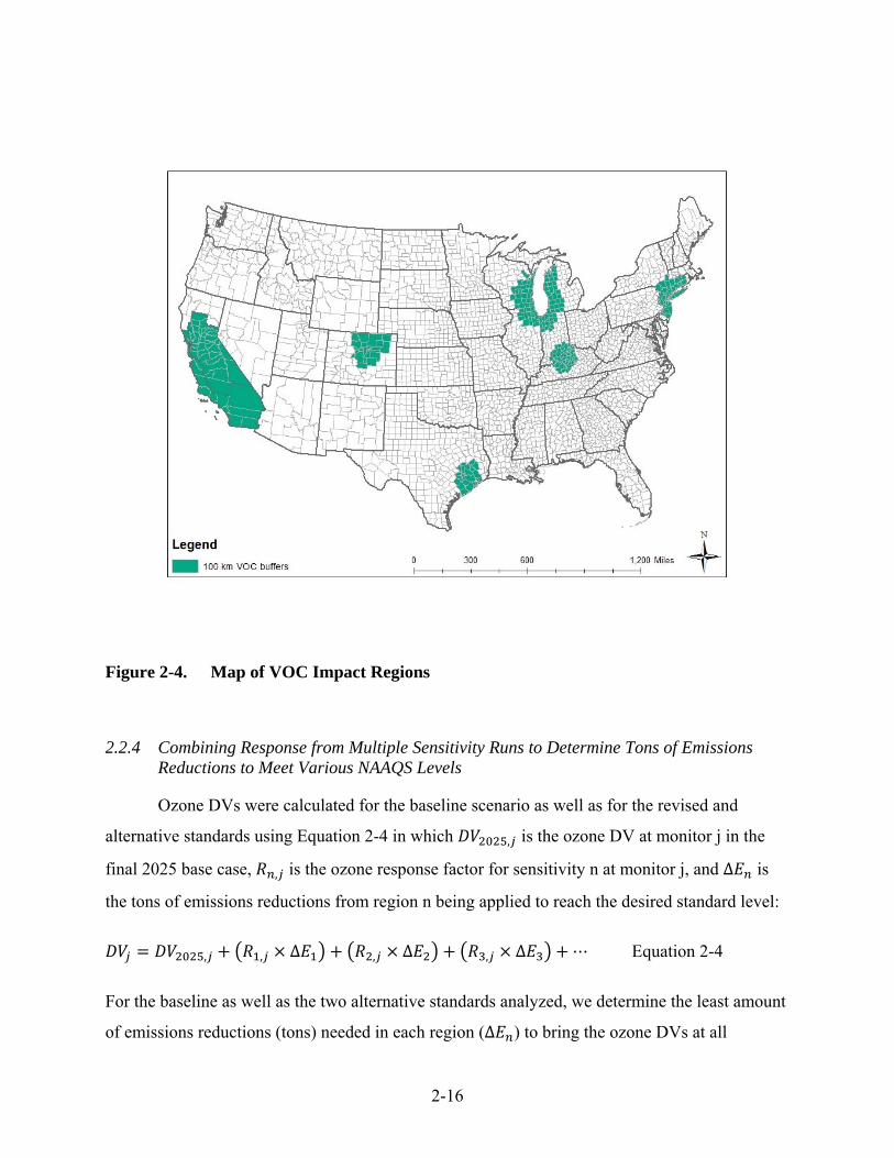
2-16
Figure 2-4. Map of VOC Impact Regions
2.2.4 Combining Response from Multiple Sensitivity Runs to Determine Tons of Emissions Reductions to Meet Various NAAQS Levels
Ozone DVs were calculated for the baseline scenario as well as for the revised and
alternative standards using Equation 2-4 in which , is the ozone DV at monitor j in the
final 2025 base case, , is the ozone response factor for sensitivity n at monitor j, and ∆ is
the tons of emissions reductions from region n being applied to reach the desired standard level:
, , ∆ , ∆ , ∆ ⋯ Equation 2-4
For the baseline as well as the two alternative standards analyzed, we determine the least amount
of emissions reductions (tons) needed in each region (∆ ) to bring the ozone DVs at all

2-17
monitors down to the particular standard level being analyzed. Note that California was analyzed
independent of the rest of the country due to the later attainment dates in many California
counties. Therefore, in determining the necessary emissions reductions, we did not account for
any impacts of California reductions on other areas of the U.S. and vice versa. The application of
equation 2-4 to determine emissions reductions necessary to meet the various standard levels at
U.S. locations outside of California is presented in chapter 3, section 3.2.
Because California included multiple incremental sensitivity simulations, Equation 2-4
had to be slightly modified for calculating DV changes to emissions reductions in that state. The
modeled impacts from multiple California sensitivity simulations were combined in a linear
manner to estimate the overall impacts. For example, at any monitor in California we could use
the following equation to determine the DVs that would result from a 75% reduction in Northern
California emissions beyond the explicit emissions control sensitivity simulation:
% , , , ∆ , ∆
, ∆ Equation 2-5
In equation 2-5, , represents the projected DV from the final 2025 base case at
monitor j, ∆ _ represents the difference in NOx emissions between the proposal
2025 base case and the 2025 California explicit emissions control sensitivity; ∆ represents
the difference in NOx emissions between the 2025 California explicit emissions control
sensitivity and the combined California explicit emissions control with 50% Northern California
NOx cuts sensitivity; and ∆ represents the additional emissions reductions needed to
reach a 75% NOx cut in Northern California above and beyond the emissions reductions in the
combined California explicit emissions control run with 50% Northern California NOx cuts run.
Note that in this equation, emission reductions in Northern California impact monitors (j) in both
the Northern and Southern California regions. Similar to the methods applied in other regions,
we determine the smallest amount of emissions reductions (tons) in northern and southern
California regions necessary to decrease all ozone DVs in each region to the standard level being
analyzed. The application of equation 2-5 to determine emissions reductions necessary to meet
the various standard levels in California is presented in chapter 3, section 3.3.

2-18
While ozone responses can be nonlinear and vary by emissions source type and location,
in this analysis we make several simplifying assumptions. First, we assume that every ton of
NOx or VOC reduced within a region results in the same ozone response regardless of where the
emissions reductions come from within the region because we do not have any information on
the differential ozone response from emissions changes at different locations within the region.
However, the somewhat smaller emissions sensitivity regions used in this analysis compared to
the November 2014 proposal RIA provide a more spatially resolved representation of the ozone
response to emissions changes and thus reduces but does not eliminate this uncertainty. Second,
we assume that NOx and VOC responses are additive. Third, we assume that the responses from
multiple regions are additive. Fourth, we assume that ozone response within each of these
sensitivity simulations is linear (i.e., the first ton of NOx reduced results in the same ozone
response as the last ton of NOx reduced). In California where we have multiple levels of
emissions reductions, we assume linearity within each simulation, but we are able to capture
discrete shifts in ozone response based on the multiple sensitivity simulations (i.e., one response
for explicit emissions control run reductions, another response level up to 50% NOx emissions
reductions beyond the explicit emissions control run, and a third level of response between 50%
and 90% NOx emissions reductions beyond the explicit emissions control run). Finally, outside
of California, the ozone response to NOx reductions greater than 50% is based on an
extrapolation beyond the modeled emissions reductions. However, only East Texas and the
Northeast require NOx reductions greater than 50% in the 65 ppb scenario and in both cases the
NOx reductions are not substantially greater than 50% (52% and 56% respectively), so we
expect that the ozone response from the 50% sensitivity is appropriate for extrapolation to 52%
and 56% with only a small amount of additional uncertainty.
2.2.5 Monitoring Sites Excluded from Quantitative Analysis
There were 1,225 ozone monitors with complete ozone data for at least one DV period
covering the years 2009-2013. We included 1,165, or 95% of these sites in the analysis to
determine the tons of emissions reductions necessary for each of the three scenarios (i.e., the
baseline and two alternative standard level scenarios). However, there were three types of sites
that were excluded from this analysis. First, we did not analyze the baseline or attainment levels
at each of the 41 sites that did not have a valid projected final 2025 base case DV because there

2-19
were fewer than 5 modeled days above 60 ppb in the 2011 CAMx simulation, as required in the
EPA SIP modeling guidance (US EPA, 2014c). It is unlikely that these sites would have any
substantial impact on costs and benefits because the reason that projections could not be made is
that they have no more than 4 modeled days above 60 ppb. Only one of these 41 sites (site
311079991 in Knox County, NE) has a base year DV greater than 65 ppb. These sites are listed
in Appendix 2A.
Second, seven sites for which the DVs were influenced by wintertime ozone episodes
were not included because the modeling tools are not currently sufficient to properly characterize
ozone formation during wintertime ozone episodes. It is not appropriate to apply the model-
based response (RRF) developed here based on summertime conditions to a wintertime ozone
event, which is driven by different characterizations of chemistry and meteorology. Since there
was no technically feasible method for projecting DVs at these sites, these sites were not
included in determining required reductions in NOx and VOCs to meet current or alternative
standard levels. Wintertime ozone events tend to be very localized phenomena driven by local
emissions from oil and gas operations (Schnell et al., 2009; Rappengluck et al., 2014; Helmig et
al., 2014). Consequently, the emissions reductions needed to lower wintertime ozone levels
would likely be different from those targeted for summertime ozone events. It follows that there
could be additional emissions reductions required to lower ozone at these locations and thus
potential additional costs and benefits that are not quantified in this analysis. Appendix 2A
includes a list of sites influenced by wintertime ozone and the methodology used to identify
those sites.
Finally, while the majority of the sites had projected ozone exceedances primarily caused
by local and regional emissions, there were a set of 12 relatively remote, rural sites in the
Western U.S. with projected baseline DVs between 66 and 69 ppb that showed limited response
to the NOx and VOC emissions sensitivities we modeled. Air agencies responsible for
attainment at these locations may choose to pursue one or more of the Clean Air Act provisions
that offer varying degrees of regulatory relief. Regulatory relief may include:
Relief from designation as a nonattainment area (through exclusion of data affected by
exceptional events)

2-20
Relief from the more stringent requirements of higher nonattainment area classifications
(through treatment as a rural transport area; through exclusion of data affected by
exceptional events; or through international transport provisions)
Relief from adopting more than reasonable controls to demonstrate attainment (through
international transport provisions)
In addition, some of these sites could potentially benefit from the CAA’s interstate transport
provisions found in sections 110(a)(2)(D) and 126. These sites were initially identified in the
November 2014 RIA proposal (EPA, 2014a) and more detailed discussion of their characteristics
were provided in Appendix 3A of that document. Only the subset of those sites with DVs
greater than 65 ppb in the 2025 baseline scenario are excluded in this analysis since sites
projected to have DVs at or below 65 ppb would not incur any additional costs or benefits.
2.3 Creating Spatial Surfaces for BenMap
The emissions reductions for attainment of the current, revised, and an alternative NAAQS
level determined in chapter 3 were used to create spatial fields of ozone concentrations (i.e.,
spatial surfaces) for input into the calculation of health benefits associated with attainment of
each NAAQS level, incremental to the baseline. The spatial surfaces used to calculate ozone-
related health benefits with the BenMap tool (Chapter 6) are described below.
Health benefits associated with meeting different ozone standard levels were calculated
based on the following three ozone metrics, as described in more detail in Chapter 6: May-Sep
seasonal mean of 8-hr daily maximum ozone, Apr-Sep seasonal mean of 1-hr daily maximum
ozone, and May-Sep seasonal mean of 9-hr daily average ozone (6am-3pm). For each metric,
spatial fields (i.e., gridded surfaces) were created for a total of 8 scenarios, including:
2025 baseline
post-2025 baseline
2025 70 ppb identified control strategies
2025 70 ppb identified + unidentified control strategies
post-2025 70 ppb identified + unidentified control strategies
2025 65 ppb identified control strategies
2025 65 ppb identified + unidentified control strategies

2-21
post-2025 65 ppb identified + unidentified control strategies
The surfaces created for the 2025 scenarios represent attainment at all contiguous U.S.
monitors outside of California, while the surfaces for the post-2025 scenarios represent all
contiguous U.S. monitors including those in California meeting the standard being evaluated.
The effects due only to California meeting the standard are isolated in Chapter 6 through a series
of BenMap simulations using these surfaces and varying assumptions about population
demographics. In addition, for the 2025 scenarios we include “identified control” and “identified
+ unidentified control” strategies in which the identified control strategies only include ozone
changes resulting from emissions reductions from identified control measures, while the
identified + unidentified controls strategies include ozone changes resulting from all emissions
reductions necessary to attain the standard from both identified controls and unidentified
measures.
The ozone surfaces were created using the following steps, which are described in more
detail below and depicted in Figure 2-5.
Step 1: Create spatial fields of gridded ozone concentrations for each of the three seasonal metrics using the model-predicted hourly ozone concentrations.
Step 2: Create spatial fields of gridded ozone response factors for each seasonal metric.
Step 3: Create spatial field of gridded ozone concentrations for baseline, revised standard, and alternative standard scenarios and each seasonal ozone metric
Step 4: Create 2011 enhanced Voronoi Neighbor Averaging (eVNA) fused surface of 2011 modeled and 2010-2012 observed values for each seasonal ozone metric
Step 5: Create eVNA fused modeled/monitored surface for each attainment scenario and each seasonal ozone metric
Step 1: Create spatial fields of seasonal ozone metrics for each model simulation
Inputs: Hourly gridded model concentrations for final 2011 base year, proposal and final 2025 base cases, and the fifteen 2025 emissions sensitivity simulations detailed in Section 2.2.2
Outputs: Seasonal ozone metrics for 2011, proposal and final 2025 base cases, and fifteen 2025 emissions sensitivity simulations (18 total spatial fields for each metric)

2-22
Step 2: Create spatial fields of ppb/ton ozone response factors
Inputs: Seasonal ozone metrics for proposal 2025 base case and fifteen 2025 emissions sensitivity simulations (from Step 1); Amount of emissions reductions (tons) modeled in each emissions sensitivity
Outputs: Gridded ozone response factor (ppb/ton) for each seasonal ozone metric from each emissions sensitivity simulation
Methods:
Calculate the change in the seasonal ozone metrics between each emissions sensitivity simulation (i) and the proposal 2025 base case. This step results in 15 spatial fields of gridded ozone changes (∆ ) for each seasonal ozone metric.
Divide each of the spatial fields of ozone changes by the tons of emissions reductions applied in that emissions sensitivity simulation compared to the
proposal 2025 base case: (∆
∆). This step results in 15 spatial fields of
gridded ozone response factors (ppb/ton) for each seasonal ozone metric.
Step 3: Create spatial field seasonal ozone metrics for baseline, revised standard, and alternative
standard scenarios
Inputs: Gridded ozone response factor for each seasonal ozone metric from each emissions sensitivity simulation (from Step 2); Amount of emissions reductions from each region (from Appendix 3A); Gridded ozone surface for each seasonal metric from the final 2025 base case (from Step 1).
Outputs: Gridded seasonal ozone metrics for each attainment scenario
Methods:
The gridded ozone response factors from Step 2 were multiplied by the relevant tons of emissions reductions for each sensitivity and then summed to create a gridded field representing the scenario using question (Equation 2-6)
3 , , 3 , , , , ∆ , , , ∆ ,
, , ∆ , ⋯ Equation 2-6

2-23
In equation 2-6, ozonexy,s,m represents the ozone concentrations at grid cell
x,y, for scenario s, and using metric, m. Similarly ozonexy,2025,m represents
the modeled ozone from the final 2025 base case simulation at grid cell x,y
aggregated to metric m. Rxy,1,m represents the ozone response factor
(ppb/ton) in grid cell x,y using metric m, for the sensitivity simulation #1.
Finally ΔE1,s represents the amount of emissions reductions from sources
modeled in sensitivity #1 that were found to be necessary for scenario s.
Identified control strategy ozone surfaces at each standard level were
created by only including ΔE values for emissions coming from identified
controls as described in Chapter 3. Post-2025 surfaces include all
emissions reductions outside of California that we estimate in 2025 plus
additional reductions in California which would occur after 2025.34
Step 4: Create 2011 enhanced Voronoi Neighbor Averaging (eVNA) fused surface of 2011
modeled and observed values for each seasonal ozone metric
Inputs: 2010-2012 observed ozone values (seasonal ozone metrics at each monitor location); 2011 modeled ozone (seasonal ozone metrics at each grid cell) (from Step 1)
Outputs: 2011 fused modeled/monitored surfaces for each seasonal ozone metric
Methods: The MATS tool was used to create a fused gridded 2011 field using both ambient and modeled data using the eVNA technique (Abt, 2014). This method essentially takes an interpolated field of observed data and adjusts it up or down based on the modeled spatial gradients. For this purpose, the 2010-2012 ambient data was interpolated and fused with the 2011 model data. One “fused” eVNA surface was created for each of the two seasonal ozone metrics.
Step 5: Create eVNA fused modeled/monitored surfaces for baseline, revised standard, and
alternative standard scenarios
34 A small error was discovered in the post-2025 surfaces in that the baseline surface included 202,000 tons of NOx emission reductions in California rather than the actual 206,000 tons of NOx emissions reductions applied to reach 75 ppb in California. This error was carried through to the 70 ppb and 65 ppb surfaces for the post-2025 scenarios so the incremental changes in ozone between the baseline and alternative NAAQS level surfaces should not be significantly impacted.

2-24
Inputs: 2011 fused model/observed surfaces for each seasonal ozone metric (from Step 4); modeled seasonal ozone metrics (gridded fields) for 2011 (from Step 1) and each attainment scenario (from Step 3).
Outputs: Fused modeled/monitored surface for each attainment scenario and each seasonal ozone metric
Methods: The 24 model-based surfaces (i.e., 8 scenarios and 3 metrics) were used as inputs in the MATS tool along with the gridded 2011 base year and eVNA surfaces. For each metric and each scenario a gridded RRF field was created by dividing the gridded ozone field for scenario s by the gridded base year 2011 model field. This RRF field was then multiplied by the 2011 eVNA field to create a gridded eVNA field for each scenario.
Figure 2-5. Process Used to Create Spatial Surfaces for BenMap
2.4 Improvements in Emissions and Air Quality for the Final RIA
2.4.1 Improvement in Emissions
Between proposal and the final rule, improvements were implemented in both the base
(2011) and future year (2025) emissions scenarios. The proposal emissions are documented in
the Version 6.1, 2011 Emissions Modeling Platform (US EPA, 2014b) TSD. Many

2-25
improvements to the inventories resulted from the Federal Register notices for the 2011 and 2018
Emissions Modeling platforms released in November 2013 and June 2014. Comments on these
notices were received from states, industry, and other organizations. Although the 2025
emissions were not specifically released for comment, improved methodologies and data were
also applied to the updated 2025 emissions wherever possible. For example, many
improvements were made on the National Electric Energy Data System database that is a key
input in the preparation of future year EGU inventories; state agencies and regional planning
organizations provided specific growth and control factors for stationary sources; and
improvements were made to the modeling of onroad mobile sources in the base and future years.
Most updates to the 2011 emissions are reflected in the 2011 National Emissions Inventory
(NEI) version 2. These updates included 1) the use of the 2014 version of the Motor Vehicle
Emissions Simulator (MOVES2014) for onroad mobile source emissions, along with many
upgrades to the input databases used by MOVES; 2) updated oil and gas emissions based on the
Oil and Gas Emissions Estimate Tool version 2.0; 3) version 3.6.1 of the Biogenic Emission
Inventory System along with improved land use data; 4) many updates to point and nonpoint
source emissions submitted directly into the Emission Inventory System (EIS) by states; 5)
improved temporal allocation of electric generating unit (EGU) and onroad mobile source
emissions; 6) upgraded VOC speciation to be consistent with the most recent chemical
mechanism available in CAMx (i.e., CB6); and 7) improved spatial surrogates for heavy-duty
trucks, buses, and other types of vehicles. In addition, Canadian emissions were upgraded to the
latest available data from Environment Canada for the year 2010 and Mexican emissions were
upgraded to use the 2008 Inventario Nacional de Emisiones de Mexico, whereas for the proposal
modeling the Mexican emissions had been based on those developed for 1999. The cumulative
national impact of the changes to 2011 emissions between the proposal and final RIA resulted in
a 1% increase in NOx emissions and no change in VOC emissions, although local changes were
larger.
Improvements to the 2025 emissions included 1) using the Integrated Planning Model
(IPM) version 5.14 with associated input databases and a representation of the Cross-State Air
Pollution Rule (CSAPR); 2) using MOVES2014 to represent emission reductions from the Tier 3
Final rulemaking and recent light and heavy duty greenhouse gas mobile source rules; 3) use of

2-26
Annual Energy Outlook (AEO) 2014 for projections of vehicle miles traveled, oil and gas
growth, and growth in other categories; and 4) improved representation of growth and controls
for non-EGU stationary source emissions. The cumulative national impact of the changes to the
2025 emissions between the proposal and final RIAs resulted in a 2% reduction in NOx
emissions and a 1% increase in VOC emissions, although localized changes were larger. For
more information on the improvements to the 2025 emissions, see Appendix 2A and the
Emissions Modeling TSD.
The net effects of the emissions inventory, model, and model input updates are changes in
projected 2025 ozone air quality design values (DVs) in many areas. These new projected DVs
were higher than previously modeled for the proposal RIA in some locations and lower in others.
The new projections show lower 2025 DVs in Central Texas from Houston to Dallas, the El Paso
area (NM and TX) and Big Bend, Texas, and several states in the central U.S., including
Oklahoma, Kansas, Missouri, Arkansas, Mississippi, Tennessee, and southern Kentucky. The
new projections also show higher 2025 DVs in Denver, Las Vegas, Phoenix, Charlotte, the upper
Midwest, and some parts of the New York/New Jersey areas. See Appendix 2A, Section 2A.4
for detailed information on the updated DVs.
2.4.2 Improvements in Air Quality Modeling
In this final RIA, we used emissions sensitivity simulations to determine the response of
ozone at monitor locations to emissions changes in specific regions, similar to the approach used
in the November 2014 proposal RIA (EPA, 2014a). However, when we reviewed the analysis
for the November 2014 proposal RIA we determined that in certain locations (e.g., Texas and the
Northeast) where violations of the 70 ppb scenario were limited to fairly localized areas, the
analysis could be improved by using more geographically refined ozone response factors. In
addition, we determined that smaller regions would also provide more refined ozone responses
across the rest of the U.S. As a result, in this final RIA we designed 10 smaller regions to
determine ozone response factors (see Figure 2-2), compared to the 5 larger regions used in the
proposal RIA (see Figure 3-3 in EPA, 2014a). This more geographically refined resolution
allows us to more accurately represent the increased effectiveness of emissions reductions closer
to monitor locations compared to emissions reductions from sources that are further away. For
example, in the proposal RIA, we analyzed one large Southwest region and made no

2-27
differentiation between the impacts of emissions from Nevada, Utah, New Mexico, Arizona, or
Colorado on the monitors in Denver. In the final RIA, the smaller regions allow us to
differentiate the impact of NOx emissions reductions in Colorado on ozone concentrations in
Denver compared to NOx emissions reductions in Arizona and New Mexico on ozone in Denver.
Similarly, in the final RIA we differentiate the impacts of east Texas emissions on ozone at
Dallas and Houston monitors from impacts of emissions in west Texas, Louisiana, Oklahoma,
Mississippi, Arkansas, Kansas and Missouri on those same monitors (in the proposal RIA, we
used one large central U.S. region that did not differentiate these impacts).
In Texas and the Northeast, the improved response factors resulted in larger changes in
ozone concentrations in response to the more geographically focused emissions reductions. For
example, in east Texas, emissions reductions were 2 to 3 times more effective at reducing ozone
concentrations at controlling monitors in Houston and Dallas than equivalent regional emissions
reductions used in the proposal. In the Northeast, local emissions reductions were 2.5 times
more effective at reducing ozone concentrations at the controlling monitor on Long Island, NY
than the equivalent regional emissions reductions used in the proposal. The more geographically
refined modeling and improved ozone response factors resulted in fewer emissions reductions
needed to meet a revised standard of 70 ppb and an alternative standard level of 65 ppb. For
additional discussion on how these improved response factors affect emissions reductions needed
to reach a revised standard of 70 ppb and an alternative standard level of 65 ppb, see Chapter 3,
Section 3.3. For additional discussion on how the improved response factors and reduced
emissions reductions impact cost estimates, see Chapter 4, Section 4.6, and for additional
discussion on how this impacts benefits estimates, see Chapter 6, Section 6.1.
2.5 References
Abt Associates, 2014. User’s Guide: Modeled Attainment Test Software. http://www.epa.gov/scram001/modelingapps_mats.htm
Dye T.S., Roberts P.T., Korc, M.E. (1995) Observations of transport processes for ozone and ozone precursors during the 1991 Lake Michigan ozone study, J. Appl. Met., 34 (8), 1877–1889
ENVIRON, 2014. User's Guide Comprehensive Air Quality Model with Extensions version 6.1, www.camx.com. ENVIRON International Corporation, Novato, CA.
Helmig, D., Thompson, C.R., Evans, J., Boylan, P., Hueber, J., Park, J.H. (2014). Highly elevated atmospheric levels of volatile organic compounds in the Uintah Basin, Utah, Environmental Science & Technology, 48, 4707-4715.

2-28
Jin, L., Tonse, S., Cohan, D. S., Mao, X. L., Harley, R. A., Brown, N. J. (2008) Sensitivity analysis of ozone formation and transport for a central California air pollution episode. Environ. Sci. Technol., 42, 3683–3689.
National Research Council (NRC), 2002. Estimating the Public Health Benefits of Proposed Air Pollution Regulations, Washington, DC: National Academies Press.
Rappengluck, B., Ackermann, L., Alvarez, S., Golovko, J., Buhr, M., Field, R.A., Soltis, J., Montague, D.C., Hauze, B., Adamson, S., Risch, D., Wilkerson, G., Bush, D., Stoeckenius, T., Keslar, C. (2014). Strong wintertime ozone events in the Upper Green River basin, Wyoming, Atmospheric Chemistry and Physics, 14, 4909-4934.
Schnell, R.C., Oltmans, S.J., Neely, R.R., Endres, M.S., Molenar, J.V., White, A.B. (2009) Rapid photochemical production of ozone at high concentrations in a rural site during winter, Nature Geoscience, 2, 120-122.
U.S. Environmental Protection Agency (2008) Final ozone NAAQS regulatory impact analysis, US EPA, OAQPS, RTP, NC, EPA-452/R-08-003
U.S. Environmental Protection Agency (2012) Regulatory Impact Analysis for the Final Revision to the National Ambient Air Quality Standards for Particulate Matter, US EPA, OAQPS, 2012, RTP, NC, EPA-452/R-12-005. http://www.epa.gov/ttnecas1/regdata/RIAs/finalria.pdf
U.S. Environmental Protection Agency (2014a) Regulatory Impact Analysis of the Proposed Revisions to the National Ambient Air Quality Standards for Ground-Level Ozone, US EPA, OAQPS, 2014, RTP, EPA-452/P-14-006, http://www.epa.gov/ttn/ecas/regdata/RIAs/20141125ria.pdf
U.S. Environmental Protection Agency (2014b) Preparation of Emissions Inventories for the Version 6.1, 2011 Emissions Modeling Platform (http://www.epa.gov/ttn/chief/emch)
U.S. Environmental Protection Agency (2014c) Draft Modeling Guidance for demonstrating attainment of air quality goals for ozone, PM2.5, and regional haze. September 2014, U.S. Environmental Protection Agency, Research Triangle Park, NC, 27711
U.S. Environmental Protection Agency (2014d) Regulatory Impact Analysis for the Proposed Carbon Pollution Guidelines for Existing Power Plants and Emission Standards for Modified and Reconstructed Power Plants, US EPA, OAQPS, 2014, RTP, NC, EPA-542/R-14-002
U.S. Environmental Protection Agency (2014e) Control Strategy Tool (CoST) Documentation Report. Office of Air Quality Planning and Standards, Research Triangle Park, NC. Available at http://www.epa.gov/ttnecas1/cost.htm.
U.S. Environmental Protection Agency (2014f) Health Risk and Exposure Assessment for Ozone, final report. US EPA, OAQPS, 2014, RTP, NC, EPA-452/R-14-004a
U.S. Environmental Protection Agency (2015) Preparation of Emissions Inventories for the Version 6.2, 2011 Emissions Modeling Platform (http://www.epa.gov/ttn/chief/emch)
2A-1
APPENDIX 2A: ADDITIONAL AIR QUALITY ANALYSIS AND RESULTS
2A.1 2011 Emissions and Air Quality Modeling Platform
2A.1.1 Photochemical Model Description and Modeling Domain
CAMx is a three-dimensional grid-based Eulerian air quality model designed to estimate
the formation and fate of oxidant precursors, primary and secondary particulate matter
concentrations, and deposition over regional and urban spatial scales (e.g., over the contiguous
U.S.) (Environ, 2014). Consideration of the different processes (e.g., transport and deposition)
that affect primary (directly emitted) and secondary (formed by atmospheric processes)
pollutants at the regional scale in different locations is fundamental to understanding and
assessing the effects of emissions control measures that affect air quality concentrations. Because
it accounts for spatial and temporal variations as well as differences in the reactivity of
emissions, CAMx is useful for evaluating the impacts of the control strategies on ozone
concentrations. CAMx is applied with the carbon-bond 6 revision 2 (CB6r2) gas-phase chemistry
mechanism (Ruiz and Yarwood, 2013).
Figure 2A-1 shows the geographic extent of the modeling domain that was used for air
quality modeling in this analysis. The domain covers the 48 contiguous states along with the
southern portions of Canada and the northern portions of Mexico. This modeling domain
contains 25 vertical layers with a top at about 17,600 meters, or 50 millibars (mb), and horizontal
resolution of 12 km x 12 km. The model simulations produce hourly air quality concentrations
for each 12 km grid cell across the modeling domain.
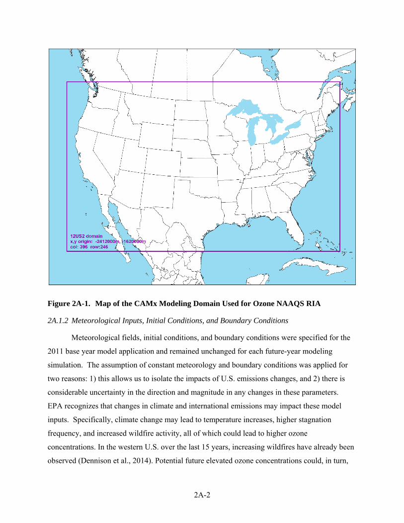
2A-2
Figure 2A-1. Map of the CAMx Modeling Domain Used for Ozone NAAQS RIA
2A.1.2 Meteorological Inputs, Initial Conditions, and Boundary Conditions
Meteorological fields, initial conditions, and boundary conditions were specified for the
2011 base year model application and remained unchanged for each future-year modeling
simulation. The assumption of constant meteorology and boundary conditions was applied for
two reasons: 1) this allows us to isolate the impacts of U.S. emissions changes, and 2) there is
considerable uncertainty in the direction and magnitude in any changes in these parameters.
EPA recognizes that changes in climate and international emissions may impact these model
inputs. Specifically, climate change may lead to temperature increases, higher stagnation
frequency, and increased wildfire activity, all of which could lead to higher ozone
concentrations. In the western U.S. over the last 15 years, increasing wildfires have already been
observed (Dennison et al., 2014). Potential future elevated ozone concentrations could, in turn,
2A-3
necessitate more stringent emissions reductions. However, there are significant uncertainties
regarding the precise location and timing of climate change impacts on ambient air quality.
Generally, climate projections are most robust for periods at least several decades in the future
because the forcing mechanisms that drive near-term natural variability in climate patterns (e.g.,
El Nino, North American Oscillation) have substantially larger signals over short time spans than
the driving forces related to long-term climate change. Boundary conditions, which are impacted
by international emissions and may also influence future ozone concentrations, are held constant
in this analysis based on a similar rationale regarding the significant uncertainty in estimating
future levels.
Meteorological inputs reflecting 2011 conditions across the contiguous U.S. were derived
from Version 3.4 of the Weather Research Forecasting Model (WRF) (Skamarock, 2008). These
inputs included hourly-varying horizontal wind components (i.e., speed and direction),
temperature, moisture, vertical diffusion rates, and rainfall rates for each grid cell in each vertical
layer. Details of the annual 2011 meteorological model simulation and evaluation are provided in
a separate technical support document (US EPA, 2014a).
The lateral boundary and initial species concentrations are provided by a three-
dimensional global atmospheric chemistry model, GEOS-Chem standard version 8-03-02
(Yantosca and Carouge, 2010) with 8-02-01 chemistry. The global GEOS-Chem model
simulates atmospheric chemical and physical processes driven by assimilated meteorological
observations from the NASA’s Goddard Earth Observing System (GEOS-5; additional
information available at: http://gmao.gsfc.nasa.gov/GEOS/ and
http://wiki.seas.harvard.edu/geos-chem/index.php/GEOS-5). This model was run for 2011 with a
grid resolution of 2.0 degrees x 2.5 degrees (latitude-longitude). The predictions were used to
provide one-way dynamic boundary conditions at one-hour intervals and an initial concentration
field for the CAMx simulations. A model evaluation was conducted to validate the
appropriateness of this version and model configuration of GEOS-Chem for predicting selected
measurements relevant to their use as boundary conditions for CAMx. This evaluation included
using satellite retrievals paired with GEOS-Chem grid cell concentrations (Henderson, 2014).
More information is available about the GEOS-Chem model and other applications using this
tool at: http://www-as.harvard.edu/chemistry/trop/geos.

2A-4
2A.1.3 2025 Base Case Emissions Inputs
CAMx requires detailed emissions inventories containing temporally allocated (i.e.,
hourly) emissions for each grid-cell in the modeling domain for a large number of chemical
species that act as primary pollutants and precursors to secondary pollutants. The annual
emission inventories were preprocessed into CAMx-ready inputs using the Sparse Matrix
Operator Kernel Emissions (SMOKE) modeling system (Houyoux et al., 2000).
The 2025 EGU projected inventory represents demand growth, fuel resource availability,
generating technology cost and performance, and other economic factors affecting power sector
behavior. The EGU emissions were developed using the IPM35 version 5.14
(http://epa.gov/powersectormodeling/psmodel514.html). IPM reflects the expected 2025
emissions accounting for the effects of environmental rules and regulations, consent decrees and
settlements, plant closures, units built, control devices installed, and forecast unit construction
through the calendar year 2025. Improvements to the National Electric Energy Data System
database, a key input in the preparation of future year EGU inventories, were implemented as a
result of updated information becoming available and based on comments submitted in response
the January 2014 Federal Register notice. In this analysis, the projected EGU emissions include
impacts from the Final Mercury and Air Toxics Standard (MATS) announced on December 21,
2011 and the CSAPR issued July 6, 2011.36
Projections for most stationary emissions sources other than EGUs (i.e., non-EGUs) were
developed by using the EPA Control Strategy Tool (CoST) to create post-controls future year
inventories. CoST is described in chapter 4 (section 4.1.1) and at
http://www.epa.gov/ttnecas1/cost.htm. The 2025 base case non-EGU stationary source emissions
inventory includes all enforceable national rules and programs including the Reciprocating
Internal Combustion Engines (RICE) and cement manufacturing National Emissions Standards
for Hazardous Air Pollutants (NESHAPs) and Boiler Maximum Achievable Control Technology
(MACT) reconsideration reductions. Projection factors and percent reductions for non-EGU
point sources reflect comments received by EPA in response to the January 2014 Federal
35 IPM is a multiregional, dynamic, deterministic linear programming model of the U.S. electric power sector. 36 An emissions modeling sensitivity run described in Section 2.2.2 also includes a representation of EPA’s proposed carbon pollution guidelines under section 111(d) of the Clean Air Act (CAA).
2A-5
Register Notice, along with emissions reductions due to national and local rules, control
programs, plant closures, consent decrees and settlements. Some improvements made based on
comments included the use of growth and control factors provided by states and by regional
organizations on behalf of states. Reductions to criteria air pollutant (CAP) emissions from
stationary engines resulting as cobenefits to the Reciprocating Internal Combustion Engines
(RICE) National Emission Standard for Hazardous Air Pollutants (NESHAP) are included.
Reductions due to the New Source Performance Standards (NSPS) VOC controls for oil and gas
sources, and the NSPS for process heaters, internal combustion engines, and natural gas turbines
are also included.
Regional projection factors for point and nonpoint oil and gas emissions were developed
using Annual Energy Outlook (AEO) 2014 projections from year 2011 to year 2025
(http://www.eia.gov/forecasts/aeo/). Projected emissions for corn ethanol, cellulosic ethanol and
biodiesel plants, refineries and upstream impacts represent the Energy Independence and
Security Act (EISA) renewable fuel standards mandate in the Renewable Fuel Standards
Program (RFS2). Airport-specific terminal area forecast (TAF) data were used for aircraft to
account for projected changes in landing/takeoff activity.
Projection factors for livestock are based on expected changes in animal population from
2005 Department of Agriculture data, updated according to EPA experts in July 2012; fertilizer
application NH3 emissions projections include upstream impacts representing EISA. Area
fugitive dust projection factors for categories related to livestock estimates are based on expected
changes in animal population and upstream impacts from EISA. Fugitive dust for paved and
unpaved roads take growth in VMT and population into account. Residential Wood Combustion
(RWC) projection factors reflect assumed growth of wood burning appliances based on sales
data, equipment replacement rates and change outs. These changes include growth in lower-
emitting stoves and a reduction in higher emitting stoves. Impacts from the New Source
Performance Standards (NSPS) for wood burning devices are also included.
Projection factors for the remaining nonpoint sources such as stationary source fuel
combustion, industrial processes, solvent utilization, and waste disposal, reflect emissions
reductions due to control programs along with comments on the growth and control of these

2A-6
sources as a result of the January 2014 Federal Register notice and information gathered from
prior rulemakings and outreach to states on emission inventories. Future year portable fuel
container (PFC) inventories reflect the impact of the final Mobile Source Air Toxics (MSAT2).
The MOVES2014-based 2025 onroad mobile source emissions account for changes in
activity data and the impact of on-the-books national rules including: the Tier 3 Vehicle
Emission and Fuel Standards Program, the 2017 and Later Model Year Light-Duty Vehicle
Greenhouse Gas Emissions and Corporate Average Fuel Economy Standards (LD GHG), the
Renewable Fuel Standard (RFS2), the Mobile Source Air Toxics Rule, the Light Duty Green
House Gas/Corporate Average Fuel Efficiency (CAFE) standards for 2012-2016, the Greenhouse
Gas Emissions Standards and Fuel Efficiency Standards for Medium- and Heavy-Duty Engines
and Vehicles, the Light-Duty Vehicle Tier 2 Rule, and the Heavy-Duty Diesel Rule. The
MOVES-based 2025 emissions also include state rules related to the adoption of LEV standards,
inspection and maintenance programs, Stage II refueling controls, and local fuel restrictions. For
California, the base case emissions included most of this state’s on-the-books regulations, such
as those for idling of heavy-duty vehicles, chip reflash, public fleets, track trucks, drayage trucks,
and heavy duty trucks and buses. The California emissions do not reflect the impacts of the
GHG/Smartway regulation, nor do they reflect state GHG regulations for the projection of other
emissions sectors because that information was not included in the provided inventories. The
input databases for MOVES, the methods for projecting activity data, and the emissions
estimation methods implemented with MOVES were improved from those used in the proposal
modeling with some improvements based on comments received via the January 2014 Federal
Register notice.
The nonroad mobile 2025 emissions, including railroads and commercial marine vessel
emissions also include all national control programs. These control programs include the Clean
Air Nonroad Diesel Rule – Tier 4, the Nonroad Spark Ignition rules, and the Locomotive-Marine
Engine rule. For ocean-going vessels (Class 3 marine), the emissions data reflect the 2005
voluntary Vessel Speed Reduction (VSR) within 20 nautical miles, the 2007 and 2008 auxiliary
engine rules, the 40 nautical mile VSR program, the 2009 Low Sulfur Fuel regulation, the 2009-
2018 cold ironing regulation, the use of 1% sulfur fuel in the Emissions Control Area (ECA)
zone, the 2012-2015 Tier 2 NOx controls, the 2016 0.1% sulfur fuel regulation in ECA zone, and

2A-7
the 2016 International Marine Organization (IMO) Tier 3 NOx controls. Control and growth-
related assumptions for 2025 came from the Emissions Modeling Platform and are described in
more detail in EPA (2014b). Non-U.S. and U.S. category 3 commercial marine emissions were
projected to 2025 using consistent methods that incorporated controls based on ECA and IMO
global NOx and SO2 controls. For California, the 2025 emissions for these categories reflect the
state’s Off-Road Construction Rule for “In-Use Diesel”, cargo handling equipment rules in place
as of 2011 (see http://www.arb.ca.gov/ports/cargo/cargo.htm), and state rules through 2011
related to Transportation Refrigeration Units, the Spark-Ignition Marine Engine and Boat
Regulations adopted on July 24, 2008 for pleasure craft, and the 2007 and 2010 regulations to
reduce emissions from commercial harbor craft.
All modeled 2011 and 2025 emissions cases use the 2010 Canada emissions data. Note
that 2010 is the latest year for which Environment Canada had provided data at the time the
modeling was performed, and no accompanying future-year projected base case inventories were
provided in a form suitable for this analysis. For Mexico, emissions compiled from the
Inventario Nacional de Emisiones de Mexico, 2008 were used for 2011, as that was the latest
complete inventory available. For 2025, projected emissions for the year 2025 based on the
2008 inventory were used (ERG, 2014). Offshore oil platform emissions for the United States
represent the year 2011 and are consistent with those in the 2011 National Emissions Inventory,
version 2. Biogenic and fire emissions were held constant for all emissions cases and were based
on 2011-specific data. Table 2A-1 shows the modeled 2011 and 2025 NOX and VOC emissions
by sector. Additional details on the emissions by state are given in the emissions modeling TSD.
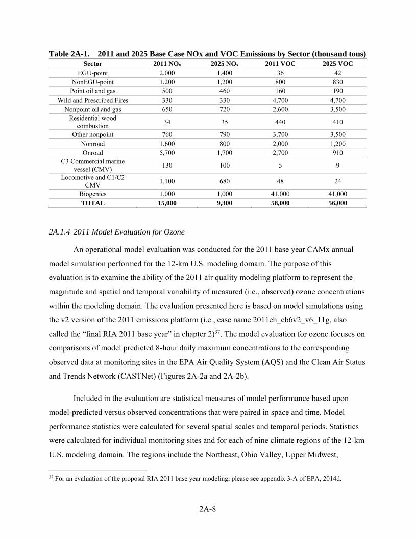
2A-8
Table 2A-1. 2011 and 2025 Base Case NOx and VOC Emissions by Sector (thousand tons) Sector 2011 NOx 2025 NOx 2011 VOC 2025 VOC
EGU-point 2,000 1,400 36 42 NonEGU-point 1,200 1,200 800 830
Point oil and gas 500 460 160 190 Wild and Prescribed Fires 330 330 4,700 4,700
Nonpoint oil and gas 650 720 2,600 3,500 Residential wood
combustion 34 35 440 410
Other nonpoint 760 790 3,700 3,500 Nonroad 1,600 800 2,000 1,200 Onroad 5,700 1,700 2,700 910
C3 Commercial marine vessel (CMV)
130 100 5 9
Locomotive and C1/C2 CMV
1,100 680 48 24
Biogenics 1,000 1,000 41,000 41,000 TOTAL 15,000 9,300 58,000 56,000
2A.1.4 2011 Model Evaluation for Ozone
An operational model evaluation was conducted for the 2011 base year CAMx annual
model simulation performed for the 12-km U.S. modeling domain. The purpose of this
evaluation is to examine the ability of the 2011 air quality modeling platform to represent the
magnitude and spatial and temporal variability of measured (i.e., observed) ozone concentrations
within the modeling domain. The evaluation presented here is based on model simulations using
the v2 version of the 2011 emissions platform (i.e., case name 2011eh_cb6v2_v6_11g, also
called the “final RIA 2011 base year” in chapter 2)37. The model evaluation for ozone focuses on
comparisons of model predicted 8-hour daily maximum concentrations to the corresponding
observed data at monitoring sites in the EPA Air Quality System (AQS) and the Clean Air Status
and Trends Network (CASTNet) (Figures 2A-2a and 2A-2b).
Included in the evaluation are statistical measures of model performance based upon
model-predicted versus observed concentrations that were paired in space and time. Model
performance statistics were calculated for several spatial scales and temporal periods. Statistics
were calculated for individual monitoring sites and for each of nine climate regions of the 12-km
U.S. modeling domain. The regions include the Northeast, Ohio Valley, Upper Midwest,
37 For an evaluation of the proposal RIA 2011 base year modeling, please see appendix 3-A of EPA, 2014d.
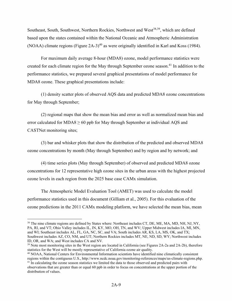
2A-9
Southeast, South, Southwest, Northern Rockies, Northwest and West38,39, which are defined
based upon the states contained within the National Oceanic and Atmospheric Administration
(NOAA) climate regions (Figure 2A-3)40 as were originally identified in Karl and Koss (1984).
For maximum daily average 8-hour (MDA8) ozone, model performance statistics were
created for each climate region for the May through September ozone season.41 In addition to the
performance statistics, we prepared several graphical presentations of model performance for
MDA8 ozone. These graphical presentations include:
(1) density scatter plots of observed AQS data and predicted MDA8 ozone concentrations
for May through September;
(2) regional maps that show the mean bias and error as well as normalized mean bias and
error calculated for MDA8 ≥ 60 ppb for May through September at individual AQS and
CASTNet monitoring sites;
(3) bar and whisker plots that show the distribution of the predicted and observed MDA8
ozone concentrations by month (May through September) and by region and by network; and
(4) time series plots (May through September) of observed and predicted MDA8 ozone
concentrations for 12 representative high ozone sites in the urban areas with the highest projected
ozone levels in each region from the 2025 base case CAMx simulation.
The Atmospheric Model Evaluation Tool (AMET) was used to calculate the model
performance statistics used in this document (Gilliam et al., 2005). For this evaluation of the
ozone predictions in the 2011 CAMx modeling platform, we have selected the mean bias, mean
38 The nine climate regions are defined by States where: Northeast includes CT, DE, ME, MA, MD, NH, NJ, NY, PA, RI, and VT; Ohio Valley includes IL, IN, KY, MO, OH, TN, and WV; Upper Midwest includes IA, MI, MN, and WI; Southeast includes AL, FL, GA, NC, SC, and VA; South includes AR, KS, LA, MS, OK, and TX; Southwest includes AZ, CO, NM, and UT; Northern Rockies includes MT, NE, ND, SD, WY; Northwest includes ID, OR, and WA; and West includes CA and NV. 39 Note most monitoring sites in the West region are located in California (see Figures 2A-2a and 2A-2b), therefore statistics for the West will be mostly representative of California ozone air quality. 40 NOAA, National Centers for Environmental Information scientists have identified nine climatically consistent regions within the contiguous U.S., http://www.ncdc.noaa.gov/monitoring-references/maps/us-climate-regions.php. 41 In calculating the ozone season statistics we limited the data to those observed and predicted pairs with observations that are greater than or equal 60 ppb in order to focus on concentrations at the upper portion of the distribution of values.
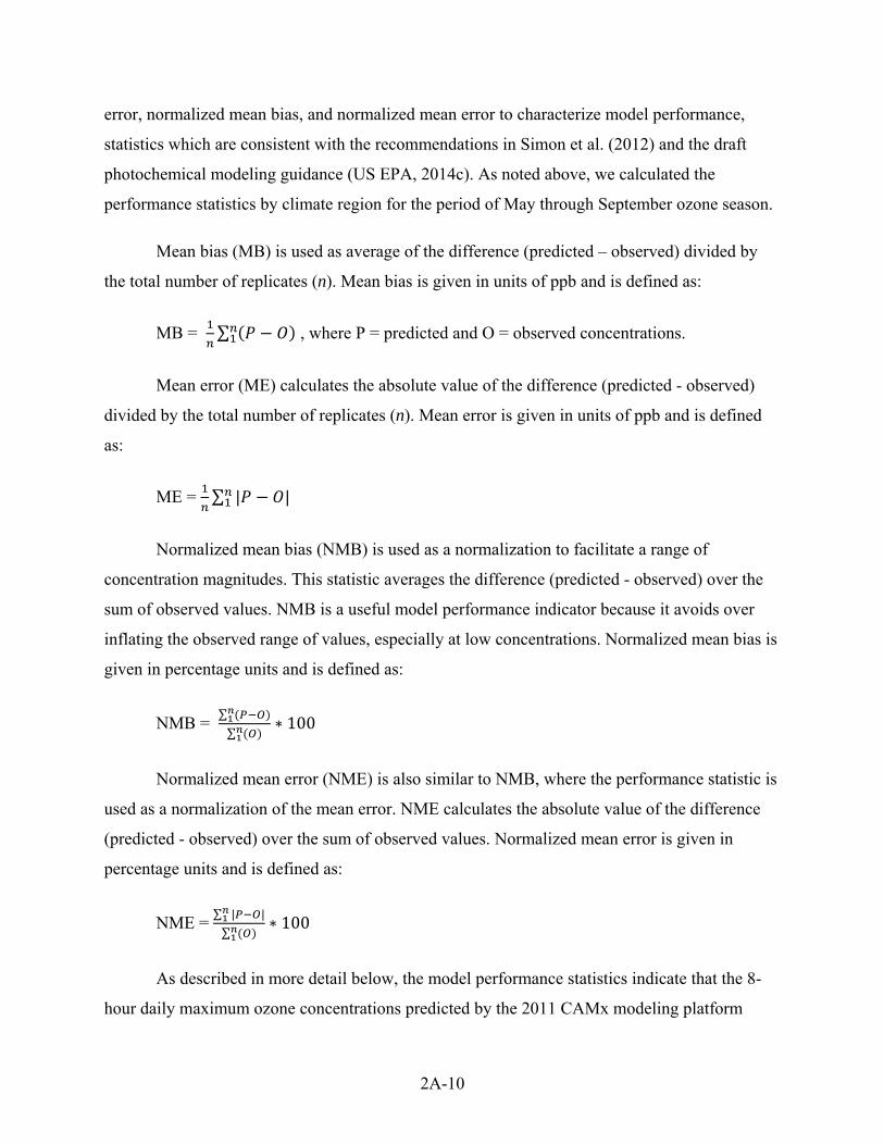
2A-10
error, normalized mean bias, and normalized mean error to characterize model performance,
statistics which are consistent with the recommendations in Simon et al. (2012) and the draft
photochemical modeling guidance (US EPA, 2014c). As noted above, we calculated the
performance statistics by climate region for the period of May through September ozone season.
Mean bias (MB) is used as average of the difference (predicted – observed) divided by
the total number of replicates (n). Mean bias is given in units of ppb and is defined as:
MB = ∑ , where P = predicted and O = observed concentrations.
Mean error (ME) calculates the absolute value of the difference (predicted - observed)
divided by the total number of replicates (n). Mean error is given in units of ppb and is defined
as:
ME = ∑ | |
Normalized mean bias (NMB) is used as a normalization to facilitate a range of
concentration magnitudes. This statistic averages the difference (predicted - observed) over the
sum of observed values. NMB is a useful model performance indicator because it avoids over
inflating the observed range of values, especially at low concentrations. Normalized mean bias is
given in percentage units and is defined as:
NMB = ∑
∑∗ 100
Normalized mean error (NME) is also similar to NMB, where the performance statistic is
used as a normalization of the mean error. NME calculates the absolute value of the difference
(predicted - observed) over the sum of observed values. Normalized mean error is given in
percentage units and is defined as:
NME = ∑ | |
∑∗ 100
As described in more detail below, the model performance statistics indicate that the 8-
hour daily maximum ozone concentrations predicted by the 2011 CAMx modeling platform

2A-11
closely reflect the corresponding 8-hour observed ozone concentrations in space and time in each
region of the 12-km U.S. modeling domain. The acceptability of model performance was judged
by considering the 2011 CAMx performance results in light of the range of performance found in
recent regional ozone model applications (NRC, 2002; Phillips et al., 2007; Simon et al., 2012;
US EPA, 2005; US EPA, 2009; US EPA, 2011). These other modeling studies represent a wide
range of modeling analyses that cover various models, model configurations, domains, years
and/or episodes, chemical mechanisms, and aerosol modules. Overall, the ozone model
performance results for the 2011 CAMx simulations are within the range found in other recent
peer-reviewed and regulatory applications. The model performance results, as described in this
document, demonstrate that the predictions from the 2011 modeling platform closely replicate
the corresponding observed concentrations in terms of the magnitude, temporal fluctuations, and
spatial differences for 8-hour daily maximum ozone.
The density scatter plots of MDA8 ozone are provided Figure 2A-4. The 8-hour ozone
model performance bias and error statistics by network for the ozone season (May-September
average) for each region are provided in Table 2A-2. The statistics shown were calculated using
data pairs on days with observed 8-hour ozone of ≥ 60 ppb. The distributions of observed and
predicted 8-hour ozone by month in the 5-month ozone season for each region are shown in
Figures 2A-5 through 2A-13. Spatial plots of the mean bias and error as well as the normalized
mean bias and error for individual monitors are shown in Figures 2A-14 through 2A-17. The
statistics shown in these two sets of figures were calculated over the ozone season using data
pairs on days with observed 8-hour ozone of ≥ 60 ppb. Time series plots of observed and
predicted 8-hour ozone during the ozone season at the 12 representative high ozone monitoring
sites are provided in Figure 2A-18, (a) through (l). These sites are listed in Table 2A-3.
The density scatter plots in Figure 2A-4 provide a qualitative comparison of model-
predicted and observed MDA8 ozone concentrations. In these plots the intensity of the colors
indicates the density of individual observed/predicted paired values. The greatest number of
individual paired values is denoted by the core area in white. The plots indicate that the
predictions correspond closely to the observations in that a large number of observed/predicted
paired values lie along or close to the 1:1 line shown on each plot. Overall, performance is best
for observed values ≥ 60. The model tends to over-predict the observed values to some extent

2A-12
particularly at low and mid-range concentrations generally < 60 ppb in each of the regions. This
feature is most evident in the South and Southeast states. In the West, high concentrations are
under-predicted and low and mid-range concentrations are over-predicted. Observed and
predicted values are in close agreement in the Southwest and Northwest regions.
As indicated by the statistics in Table 2A-2, bias and error for 8-hour daily maximum
ozone are relatively low in each region. Generally, MB for 8-hour ozone ≥ 60 ppb during the
ozone season is less than 5 ppb except at AQS sites in the Western region and at rural CASTNet
sites in the South, Southwest and Western regions for which ozone is somewhat under-predicted.
The monthly distribution of 8-hour daily maximum ozone during the ozone season generally
corresponds well with that of the observed concentrations, as indicated by the graphics in Figures
2A-5 through 2A-13. The distribution of predicted concentrations tends to be close to that of the
observed data at the 25th percentile, median and 75th percentile values for each region, although
there is a small persistent overestimation bias for these metrics in the Northeast, Southeast, and
Ohio Valley regions, and under-prediction at CASTNet sites in the West and Southwest42. The
CAMx model, as applied here, also has a tendency to under-predict the highest observational
concentrations at both the AQS and CASTNet network sites.
Figures 2A-14 through 2A-17 show the spatial variability in bias and error at monitor
locations. Mean bias, as seen from Figure 2A-14, is less than 5 ppb at many sites across the East
with over-prediction of 5 to 10 ppb at some sites from the Southeast into the Northeast.
Elsewhere, mean bias is generally in the range of -5 to -10 ppb. Figure 2A-15 indicates that the
normalized mean bias for days with observed 8-hour daily maximum ozone greater than or equal
to 60 ppb is within ± 10 percent at the vast majority of monitoring sites across the modeling
domain. There are regional differences in model performance, where the model tends to over-
predict from the Southeast into the Northeast and generally under predict in the Southwest,
Northern Rockies, Northwest and West. Model performance in the Ohio Valley and Upper
Midwest states shows both under and over predictions.
42 The over-prediction at CASTNet sites in the Northwest may not be representative of performance in rural areas of this region because there are so few observed and predicted data pairs in this region.

2A-13
Model error, as seen from Figure 2A-16, is 10 ppb or less at most of the sites across the
modeling domain. Figure 2A-17 indicates that the normalized mean error for days with observed
8-hour daily maximum ozone greater than or equal to 60 ppb is within 10 percent at the vast
majority of monitoring sites across the modeling domain. Somewhat greater error (i.e., greater
than 15 percent) is evident at sites in several areas most notably along portions of the Northeast
and in portions of Florida, North Dakota, Illinois, Ohio, North Carolina, and the western most
part of the modeling domain.
In addition to the above analysis of overall model performance, we also examine how
well the modeling platform replicates day to day fluctuations in observed 8-hour daily maximum
concentrations at 12 high ozone monitoring sites. For this site-specific analysis we present the
time series of observed and predicted 8-hour daily maximum concentrations by site over the
ozone season, May through September. These monitors were chosen because they are high ozone
sites in those urban areas with the highest projected ozone levels in the 2025 base case
simulation. The results, as shown in Figures 2A-18 (a) through (l), indicate that the modeling
platform replicates the day-to-day variability in ozone during this time period. For example,
several of the sites not only have minimal bias but also accurately capture the day-to-day
variability in the observations: Alleghany County, PA; Wayne County, MI; Jefferson County,
KY. Many additional sites generally track well and capture day-to-day variability but
underestimate some of the peak ozone days: Tarrant County, TX; Brazoria County, TX; Queens
County, NY; Suffolk County, NY; Sheboygan County, WI. Note that at the site in Brazoria
County, TX there is an extended period from mid-July to mid-August with very low observed
ozone concentrations, mostly in the range of 30 to 40 ppb. The model predicted values during
this period in the range of 40 to 60 ppb which is not quite as low as the observed values. The
sites in Douglas County, CO and Harford County, MD closely track the day-to-day variability in
the observed MDA8 values, but some days are over predicted while other days are under
predicted to some extent. Finally, the daily modeled ozone at the two California sites evaluated
correlates well with observations but has a persistent low bias. Looking across all 12 sites
indicates that the modeling platform is able to capture the site to site differences in the short-term
variability of ozone concentrations.

2A-14
Figure 2A-2a. AQS Ozone Monitoring Sites
Figure 2A-2b. CASTNet Ozone Monitoring Sites

2A-15
Figure 2A-3. NOAA Nine Climate Regions (source: http://www.ncdc.noaa.gov/monitoring-references/maps/us-climate-regions.php#references)
Table 2A-2. MDA8 Ozone Performance Statistics Greater than or Equal to 60 Ppb for May through September by Climate Region, by Network
Network Climate region No. of Obs MB ME
NMB (%)
NME (%)
AQS
Northeast 3,998 2.2 7.4 3.2 10.8
Ohio Valley 6,325 0.3 7.6 0.4 11.3
Upper Midwest 1,162 -3.0 7.5 -4.4 11.0
Southeast 37,280 -2.5 8.1 -3.6 11.9
South 5,694 -3.7 8.1 -5.4 11.7
Southwest 6,033 -5.2 7.9 -7.8 12.0
Northern Rockies 380 -5.9 7.4 -9.4 11.7
Northwest 79 -5.4 8.1 -8.5 12.6
West 8,665 -7.3 9.5 -10.3 13.5
CASTNet
Northeast 264 2.3 6.1 3.4 9.1
Ohio Valley 107 -2.3 6.2 -3.4 9.4
Upper Midwest 38 -3.9 5.9 -5.8 8.8
Southeast 2,068 -5.0 8.2 -7.5 12.1
South 215 -7.1 8.0 -10.7 12.0
Southwest 382 -7.7 8.6 -11.7 13.1
Northern Rockies 110 -7.8 8.1 -12.2 12.8
Northwest - - - - -
West 425 -12.1 12.5 -16.6 17.1

2A-16
Figure 2A-4. Density Scatter Plots of Observed/Predicted MDA8 Ozone for the Northeast, Ohio River Valley, Upper Midwest, Southeast, South, Southwest, Northern Rockies, Northwest and West Regions
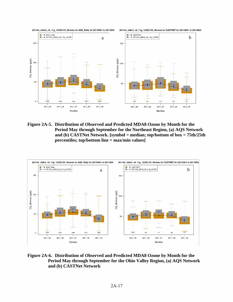
2A-17
Figure 2A-5. Distribution of Observed and Predicted MDA8 Ozone by Month for the Period May through September for the Northeast Region, (a) AQS Network and (b) CASTNet Network. [symbol = median; top/bottom of box = 75th/25th percentiles; top/bottom line = max/min values]
Figure 2A-6. Distribution of Observed and Predicted MDA8 Ozone by Month for the Period May through September for the Ohio Valley Region, (a) AQS Network and (b) CASTNet Network
b a
b a

2A-18
Figure 2A-7. Distribution of Observed and Predicted MDA8 Ozone by Month for the Period May through September for the Upper Midwest Region, (a) AQS Network and (b) CASTNet Network
Figure 2A-8. Distribution of Observed and Predicted MDA8 Ozone by Month for the Period May through September for the Southeast Region, (a) AQS Network and (b) CASTNet Network
b a
b a

2A-19
Figure 2A-9. Distribution of Observed and Predicted MDA8 Ozone by Month for the Period May through September for the South Region, (a) AQS Network and (b) CASTNet Network
Figure 2A-10. Distribution of Observed and Predicted MDA8 Ozone by Month for the Period May through September for the Southwest Region, (a) AQS Network and (b) CASTNet Network
b a
b a

2A-20
Figure 2A-11. Distribution of Observed and Predicted MDA8 Ozone by Month for the Period May through September for the Northern Rockies Region, (a) AQS Network and (b) CASTNet Network
Figure 2A-12. Distribution of Observed and Predicted MDA8 Ozone by Month for the Period May through September for the Northwest Region, (a) AQS Network and (b) CASTNet Network
b a
b a

2A-21
Figure 2A-13. Distribution of Observed and Predicted MDA8 Ozone by Month for the Period May through September for the West Region, (a) AQS Network and (b) CASTNet Network
Figure 2A-14. Mean Bias (ppb) of MDA8 Ozone Greater than or Equal to 60 ppb over the Period May-September 2011 at AQS and CASTNet Monitoring
b a

2A-22
Figure 2A-15. Normalized Mean Bias (%) of MDA8 Ozone Greater than or Equal to 60 ppb over the Period May-September 2011 at AQS and CASTNet Monitoring Sites
Figure 2A-16. Mean Error (ppb) of MDA8 Ozone Greater than or Equal to 60 ppb over the Period May-September 2011 at AQS and CASTNet Monitoring Sites
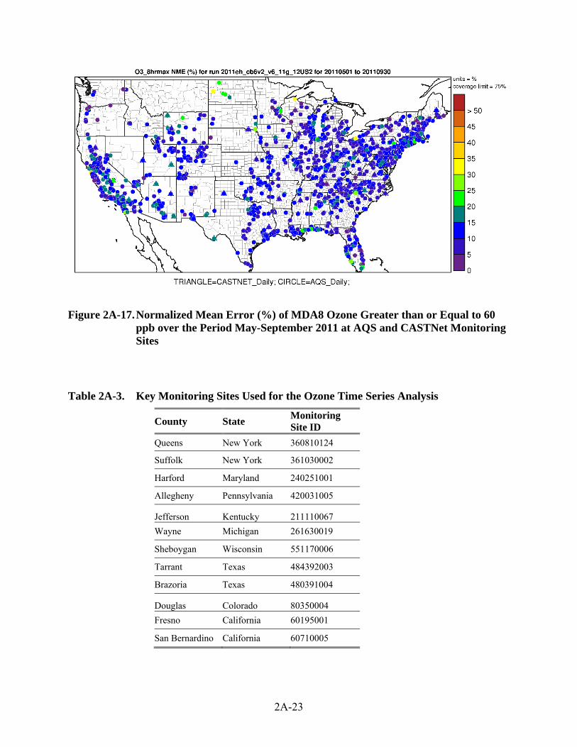
2A-23
Figure 2A-17. Normalized Mean Error (%) of MDA8 Ozone Greater than or Equal to 60 ppb over the Period May-September 2011 at AQS and CASTNet Monitoring Sites
Table 2A-3. Key Monitoring Sites Used for the Ozone Time Series Analysis
County State Monitoring Site ID
Queens New York 360810124
Suffolk New York 361030002
Harford Maryland 240251001
Allegheny Pennsylvania 420031005
Jefferson Kentucky 211110067
Wayne Michigan 261630019
Sheboygan Wisconsin 551170006
Tarrant Texas 484392003
Brazoria Texas 480391004
Douglas Colorado 80350004
Fresno California 60195001
San Bernardino California 60710005

2A-24
Figure 2A-18a. Time Series of Observed (black) and Predicted (red) MDA8 Ozone for May through September 2011 at Site 360810124 in Queens, New York
Figure 2A-18b. Time Series of Observed (black) and Predicted (red) MDA8 Ozone for May through September 2011 at Site 361030002 in Suffolk County, New York

2A-25
Figure 2A-18c. Time Series of Observed (black) and Predicted (red) MDA8 Ozone for May through September 2011 at Site 240251001 in Harford Co., Maryland
Figure 2A-18d. Time Series of Observed (black) and Predicted (red) MDA8 Ozone for May through September 2011 at Site 420031005 in Allegheny Co., Pennsylvania

2A-26
Figure 2A-18e. Time Series of Observed (black) and Predicted (red) MDA8 Ozone for May through September 2011 at Site 211110067 in Jefferson Co., Kentucky
Figure 2A-18f. Time Series of Observed (black) and Predicted (red) MDA8 Ozone for May through September 2011 at Site 261630019 in Wayne Co., Michigan

2A-27
Figure 2A-18g. Time Series of Observed (black) and Predicted (red) MDA8 Ozone for May through September 2011 at Site 551170006 in Sheboygan Co., Wisconsin
Figure 2A-18h. Time Series of Observed (black) and Predicted (red) MDA8 Ozone for May through September 2011 at Site 484392003 in Tarrant Co., Texas
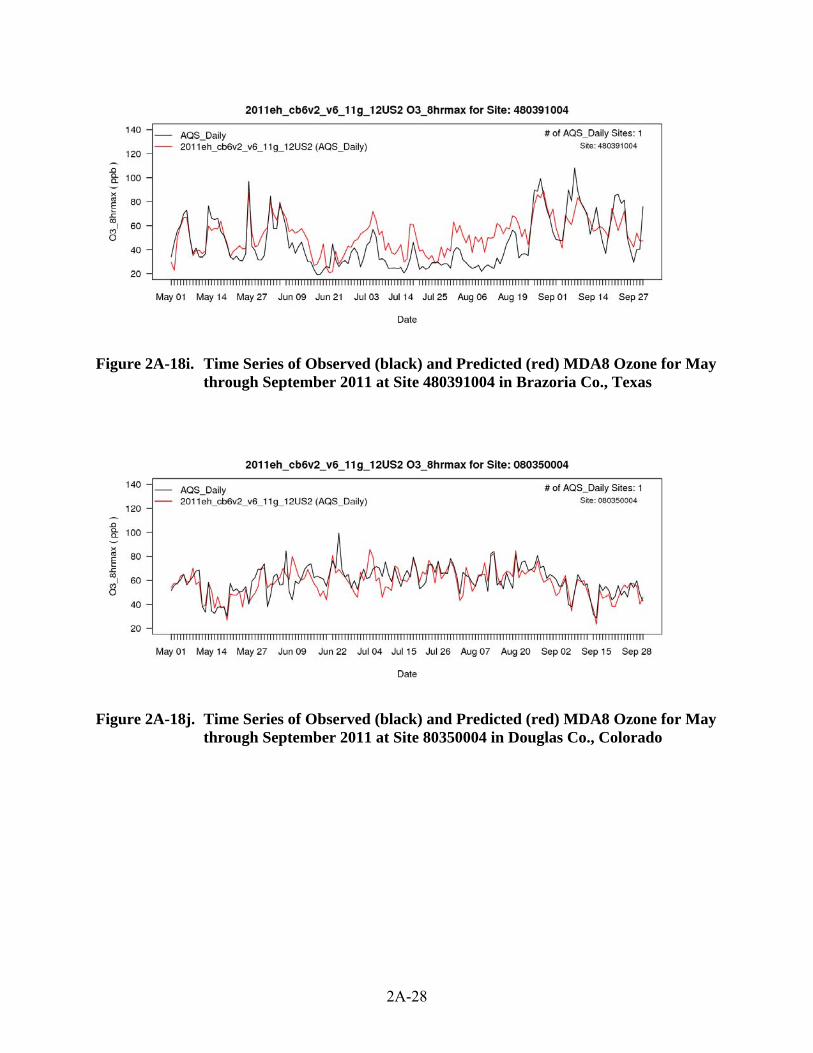
2A-28
Figure 2A-18i. Time Series of Observed (black) and Predicted (red) MDA8 Ozone for May through September 2011 at Site 480391004 in Brazoria Co., Texas
Figure 2A-18j. Time Series of Observed (black) and Predicted (red) MDA8 Ozone for May through September 2011 at Site 80350004 in Douglas Co., Colorado

2A-29
Figure 2A-18k. Time Series of Observed (black) and Predicted (red) MDA8 Ozone for May through September 2011 at Site 60195001 in Fresno Co., California
Figure 2A-18l. Time Series of Observed (black) and Predicted (red) MDA8 Ozone for May through September 2011 at Site 60710005 in San Bernardino Co., California

2A-30
2A.2 VOC Impact Regions
As described in Chapter 2, we defined VOC impact regions for the following urban areas: New
York City, Chicago, Louisville, Houston, Denver, Northern California and Southern California.43
Not only did these areas have the highest design values in each region, but ozone in these areas
was also sensitive to VOC emissions reductions in our modeling. Figure 2A-19 shows the
impact of 50% U.S. anthropogenic VOC cuts on July monthly average 8-hour daily maximum
ozone concentrations across the US. Ozone in each of the areas listed above is shown to have at
least 0.2 ppb response to VOC emissions cuts.
Figure 2A-19. Change in July Average of 8-hr Daily Maximum Ozone Concentration (ppb) Due to 50% Cut in U.S. Anthropogenic VOC Emissions
2A.3 Monitors Excluded from the Quantitative Analysis
There were 1,225 ozone monitors with complete ozone data for at least one DV period
covering the years 2009-2013. Of those sites, we quantitatively analyzed 1,165 in this analysis.
As discussed in Chapter 2, 60 sites were excluded from the quantitative analysis of emissions
43 Other local VOC areas that had similar levels of ozone response to the 50% VOC reduction were also explored but were found not to be helpful in reaching alternative NAAQS levels in this analysis: Dallas, Detroit, Pittsburgh, and Baltimore. This may be due to the construct of the attainment scenarios explored here and does not mean that VOC controls might not be effective in these areas under alternate assumptions about regional NOx controls.

2A-31
reductions needed to reach alternative standard levels. These sites fall into one of three
categories, as discussed in more detail in the following three subsections.
2A.3.1 Sites without Projections Due to Insufficient Days
Some monitors were excluded from the analysis because no future design value could be
projected at the site. This occurred when there were not enough modeled high ozone days (4 or
fewer) at the site to compute a design value according to EPA SIP modeling guidance (US EPA,
2014c). A list of the 41 sites in this category is given in Table 2A-4.
Table 2A-4. Monitors without Projections due to Insufficient High Modeling Days to Meet EPA Guidance for Projecting Design Values
Site ID Lat Long State County
60010009 37.74307 -122.17 California Alameda
60010011 37.81478 -122.282 California Alameda
60131004 37.9604 -122.357 California Contra Costa
60231004 40.77694 -124.178 California Humboldt
60450008 39.14566 -123.203 California Mendocino
60750005 37.76595 -122.399 California San Francisco
60811001 37.48293 -122.203 California San Mateo
60932001 41.72689 -122.634 California Siskiyou
160230101 43.46056 -113.562 Idaho Butte
230031100 46.69643 -68.033 Maine Aroostook
260330901 46.49361 -84.3642 Michigan Chippewa
270052013 46.85181 -95.8463 Minnesota Becker
270177416 46.70527 -92.5238 Minnesota Carlton
270750005 47.94862 -91.4956 Minnesota Lake
270834210 44.4438 -95.8179 Minnesota Lyon
271370034 48.41333 -92.8306 Minnesota Saint Louis
300298001 48.51017 -113.997 Montana Flathead
300490004 46.8505 -111.987 Montana Lewis and Clark
311079991 42.8292 -97.854 Nebraska Knox
380070002 46.8943 -103.379 North Dakota Billings
380130004 48.64193 -102.402 North Dakota Burke
380150003 46.82543 -100.768 North Dakota Burleigh
380171004 46.93375 -96.8554 North Dakota Cass
380250003 47.3132 -102.527 North Dakota Dunn
380530002 47.5812 -103.3 North Dakota McKenzie
380570004 47.29861 -101.767 North Dakota Mercer
380650002 47.18583 -101.428 North Dakota Oliver
410170122 44.0219 -121.26 Oregon Deschutes

2A-32
Site ID Lat Long State County
410290201 42.22989 -122.788 Oregon Jackson
410591003 45.82897 -119.263 Oregon Umatilla
460110003 44.3486 -96.8073 South Dakota Brookings
530090013 48.29786 -124.625 Washington Clallam
530330080 47.56824 -122.309 Washington King
530530012 46.7841 -121.74 Washington Pierce
530531010 46.75833 -122.124 Washington Pierce
530570020 48.39779 -122.505 Washington Skagit
530730005 48.95074 -122.554 Washington Whatcom
550030010 46.602 -90.656 Wisconsin Ashland
551250001 46.052 -89.653 Wisconsin Vilas
560390008 43.67083 -110.599 Wyoming Teton
560391011 44.55972 -110.401 Wyoming Teton
2A.3.2 Winter Ozone
High winter ozone concentrations that have been observed in mountain valleys in the
Western U.S. are believed to result from the combination of strong wintertime inversions, large
NOx and VOC emissions from nearby oil and gas operations, increased UV intensity due to
reflection off of snow surfaces, and potentially still uncharacterized sources of free radicals.
Current modeling tools are not sufficient to properly characterize ozone formation for these
winter ozone episodes due to (1) the challenging task of capturing complex local “cold pool”
meteorology using a model resolution that is optimized to capture regional and synoptic scale
process, (2) uncertainties in quantifying the local emissions from oil and gas operations, and (3)
uncertainties in the chemistry that occurs both in the atmosphere and on snow surfaces during
these episodes. Therefore, it was not appropriate to project ozone design values at monitors
impacted by winter events. To identify sites impacted by winter events, we examined the
ambient data that went into creating the 2009-2013 5-year weighted design value in locations
known to have conditions conducive to winter ozone formation (i.e., all sites in Wyoming, Utah,
and Colorado). At these sites, we evaluated the four highest 8-hr daily maximum ozone values in
each year from 2009-2013 to identify wintertime ozone episodes. A site was categorized as
having a design value impacted by wintertime ozone if at least 20% of the days examined (4 out
20) had ozone values greater than or equal to 75 ppb and occurred during a “winter” month

2A-33
(November-March). The seven sites identified as being affected by wintertime ozone events are
listed in Table 2A-5.
Table 2A-5. Monitors Determined to Have Design Values Affected by Winter Ozone Events
Site ID lat long State County
# of summer DV days* >= 75
# of winter DV days* >= 75
highest winter 8-hr daily max
2009-2013 DV
081030006 40.09 -108.76 Colorado Rio Blanco
0 7 106 71
560130099 42.53 -108.72 Wyoming Fremont 1 4 93 67
560350097 42.98 -110.35 Wyoming Sublette 0 3 83 64
560350099 42.72 -109.75 Wyoming Sublette 0 4 123 77
560350100 42.79 -110.06 Wyoming Sublette 0 4 84 67
560350101 42.87 -109.87 Wyoming Sublette 0 4 89 66
560351002 42.37 -109.56 Wyoming Sublette 0 4 94 68
*DV days defined here are the days with the 4 highest 8-hr daily maximum ozone values in each year from 2009-2013 (20 days). 2A.3.3 Monitoring Sites in Rural/Remote Areas of the West and Southwest
As mentioned in Chapter 2, model-predicted ozone concentrations at 12 sites in
rural/remote areas in the West and Southwest were excluded from the quantitative analysis.
These 12 sites are a subset of 26 sites identified in the November 2014 RIA proposal (US EPA,
2014d). The original 26 sites had two common characteristics. First, they had small modeled
responses to large regional NOx and VOC reductions in 2025 compared to other sites in the
region. Second, these monitors would have DVs that remain above the standard after applying
reductions needed to bring large urban areas in the region into attainment. All of these 12
monitoring sites have 2025 baseline concentrations below 70 ppb. Therefore, no emissions
reductions would be required for these sites to meet a primary standard of 70 ppb in 2025. Of
the 26 sites identified in the RIA proposal, only the sites with 2025 baseline DVs (or post-2025
baseline DVs for CA) above 65 ppb are excluded from this analysis. More details on these 12
sites are provided in Table 2A-6. We have qualitatively characterized the predominant ozone
influence for each site in Table 2A-6. These qualitative characterizations are based on the
modeled response to large regional NOx reductions in 2025, proximity to the Mexican border
(i.e., potential influence from trans-border pollution) and altitude (e.g., potential influence of
ozone transported from the free troposphere: stratospheric intrusions or long range transport of

2A-34
international anthropogenic ozone). Figure 2A-20 shows the location of all sites listed in Table
2A-7 and for demonstrative purposes assigns each site to a category based on the predominant
source of ozone in that location. The table and figure indicate that all 12 sites have 2025 or post-
2025 baseline design values below 70 ppb as mentioned above. Of the 12 sites, 5 sites are
characterized as border sites, 5 sites are characterized as being strongly influenced by California
emissions, and 2 sites are influenced by other ozone sources.
Table 2A-6. Monitors with Limited Response to Regional NOx and National VOC Emissions Reductions in the 2025 and Post-2025 Baselines
Name Site ID State County Altitude (m)
Monitor Type
Predominant O3 Sources
2009-2013 DV
Baseline DV
Chiricahua NM 40038001 Arizona Cochise 1570 CASTNET Mexican border 72 67
Grand Canyon NP 40058001 Arizona Coconino 2152 CASTNET California + Other sources
71 66
Yuma Supersite 40278011 Arizona Yuma 51 SLAMS Mexican border + California
75 66
El Centro-9th st 60251003 California Imperial - SLAMS California + Mexican Border
81 68
Yosemite NP 60430003 California Mariposa 5265 CASTNET California + Other sources
77 67
Sequoia and Kings Canyon NP
61070006 California Tulare 1890 Non-EPA Federal (NPS)
California + Other sources
81 69
Weminuche Wilderness Area
80671004 Colorado La Plata 2367 Non-EPA Federal (USFS)
Southwest region + Other sources
72 68
Great Basin NP 320330101 Nevada White Pine 2060 CASTNET California + Other sources
72 66
BLM land near Carlsbad
350151005 New Mexico
Eddy 780 SLAMS
Central region + Southwest region + Mexican border
70 67
Big Bend NP 480430101 Texas Brewster 1052 CASTNET Mexican border 70 68
BLM Land/Carlsbad
483819991 Texas Randall 780 SLAMS Central region + Mexican border + Other sources
73 66
Zion NP 490530130 Utah Washington 1213 Non-EPA Federal (NPS)
California + Other sources
71 66
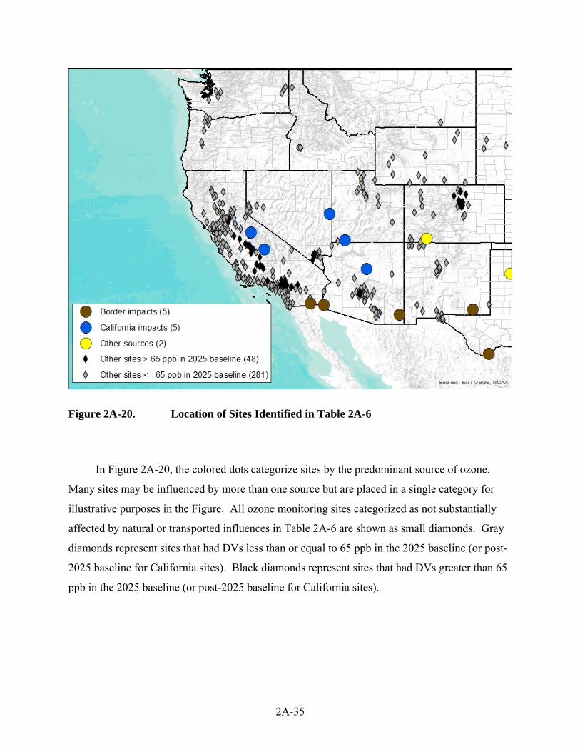
2A-35
Figure 2A-20. Location of Sites Identified in Table 2A-6
In Figure 2A-20, the colored dots categorize sites by the predominant source of ozone.
Many sites may be influenced by more than one source but are placed in a single category for
illustrative purposes in the Figure. All ozone monitoring sites categorized as not substantially
affected by natural or transported influences in Table 2A-6 are shown as small diamonds. Gray
diamonds represent sites that had DVs less than or equal to 65 ppb in the 2025 baseline (or post-
2025 baseline for California sites). Black diamonds represent sites that had DVs greater than 65
ppb in the 2025 baseline (or post-2025 baseline for California sites).

2A-36
2A.4 Design Values for All Monitors Included in the Quantitative Analysis
In addition to other information, Tables 2A-7 and 2A-8 provide baseline design values
corresponding to the information presented in the maps in Figures 3-5 and 3-11. Note that some
counties contain more than one monitor and the highest monitor is used for the map.
Table 2A-7. Design Values (ppb) for California Monitors
Site ID Lat Long State County O3 DV for Scenario:
Base Case
Baseline 70 65
60010007 37.68753 -121.784 California Alameda 67 62 58 54
60012001 37.65446 -122.032 California Alameda 54 50 48 45
60050002 38.33991 -120.764 California Amador 60 55 51 47
60070007 39.71404 -121.619 California Butte 61 56 52 48
60070008 39.76154 -121.842 California Butte 53 49 46 43
60090001 38.20185 -120.682 California Calaveras 63 57 54 50
60111002 39.20294 -122.018 California Colusa 53 49 46 43
60130002 37.93601 -122.026 California Contra Costa 66 61 57 53
60131002 38.00631 -121.642 California Contra Costa 64 58 55 51
60170010 38.72528 -120.822 California El Dorado 66 60 55 50
60170012 38.81161 -120.033 California El Dorado 62 59 57 56
60170020 38.89094 -121.003 California El Dorado 66 60 55 50
60190007 36.70551 -119.742 California Fresno 82 74 70 65
60190011 36.78532 -119.774 California Fresno 81 73 69 64
60190242 36.84139 -119.874 California Fresno 81 75 70 66
60192009 36.63423 -120.382 California Fresno 64 59 55 52
60194001 36.5975 -119.504 California Fresno 77 69 65 60
60195001 36.81911 -119.717 California Fresno 83 75 70 65
60210003 39.53376 -122.192 California Glenn 56 52 49 46
60250005 32.67619 -115.484 California Imperial 71 63 62 61
60254003 33.0325 -115.624 California Imperial 66 56 54 53
60254004 33.21361 -115.545 California Imperial 64 53 52 50
60270101 36.50861 -116.848 California Inyo 67 64 63 63
60290007 35.34609 -118.852 California Kern 80 74 69 64
60290008 35.05444 -119.404 California Kern 75 69 65 61
60290011 35.05055 -118.147 California Kern 71 62 60 57
60290014 35.35609 -119.041 California Kern 77 70 66 61
60290232 35.43887 -119.017 California Kern 76 70 66 61
60295002 35.23668 -118.789 California Kern 74 67 63 59
60296001 35.50359 -119.273 California Kern 74 68 65 61
60311004 36.3144 -119.645 California Kings 74 68 63 59
60333001 39.0327 -122.922 California Lake 50 47 44 42
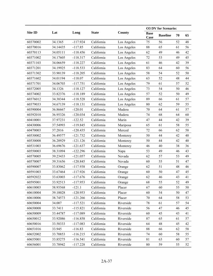
2A-37
Site ID Lat Long State County O3 DV for Scenario:
Base Case
Baseline 70 65
60370002 34.1365 -117.924 California Los Angeles 75 56 52 48
60370016 34.14435 -117.85 California Los Angeles 88 65 61 56
60370113 34.05111 -118.456 California Los Angeles 62 49 46 42
60371002 34.17605 -118.317 California Los Angeles 72 53 49 45
60371103 34.06659 -118.227 California Los Angeles 61 46 42 39
60371201 34.19925 -118.533 California Los Angeles 83 64 60 56
60371302 33.90139 -118.205 California Los Angeles 58 54 52 50
60371602 34.01194 -118.07 California Los Angeles 63 52 48 44
60371701 34.06703 -117.751 California Los Angeles 79 61 57 52
60372005 34.1326 -118.127 California Los Angeles 73 54 50 46
60374002 33.82376 -118.189 California Los Angeles 57 52 50 49
60376012 34.38344 -118.528 California Los Angeles 89 66 61 57
60379033 34.67139 -118.131 California Los Angeles 80 62 59 55
60390004 36.86667 -120.01 California Madera 70 64 61 57
60392010 36.95326 -120.034 California Madera 74 68 64 60
60410001 37.97231 -122.52 California Marin 47 44 42 39
60430006 37.54993 -119.845 California Mariposa 65 61 58 55
60470003 37.2816 -120.435 California Merced 72 66 62 58
60530002 36.49577 -121.732 California Monterey 50 44 42 40
60530008 36.20929 -121.126 California Monterey 50 44 42 40
60531003 36.69676 -121.637 California Monterey 46 40 38 36
60550003 38.31094 -122.296 California Napa 53 49 46 43
60570005 39.23433 -121.057 California Nevada 62 57 53 49
60570007 39.31656 -120.845 California Nevada 60 55 51 47
60590007 33.83062 -117.938 California Orange 62 51 48 46
60591003 33.67464 -117.926 California Orange 60 50 47 45
60592022 33.63003 -117.676 California Orange 62 46 43 41
60595001 33.92513 -117.953 California Orange 68 55 52 49
60610003 38.93568 -121.1 California Placer 67 60 55 50
60610004 39.10028 -120.953 California Placer 60 54 50 47
60610006 38.74573 -121.266 California Placer 70 64 58 53
60650004 34.007 -117.521 California Riverside 78 61 57 54
60650008 33.7411 -115.821 California Riverside 56 47 46 45
60650009 33.44787 -117.089 California Riverside 60 45 43 41
60650012 33.92086 -116.858 California Riverside 87 65 61 57
60650016 33.58333 -117.083 California Riverside 64 48 45 42
60651016 33.945 -116.83 California Riverside 88 66 62 58
60652002 33.70853 -116.215 California Riverside 74 60 58 55
60655001 33.85275 -116.541 California Riverside 81 63 60 57
60656001 33.78942 -117.228 California Riverside 80 59 55 52

2A-38
Site ID Lat Long State County O3 DV for Scenario:
Base Case
Baseline 70 65
60658001 33.99958 -117.416 California Riverside 88 67 63 58
60658005 33.99564 -117.493 California Riverside 84 64 60 56
60659001 33.67649 -117.331 California Riverside 75 55 52 49
60659003 33.61241 -114.603 California Riverside 60 54 53 52
60670002 38.71209 -121.381 California Sacramento 66 60 55 50
60670006 38.61378 -121.368 California Sacramento 67 61 56 51
60670010 38.55823 -121.493 California Sacramento 62 57 52 48
60670011 38.30259 -121.421 California Sacramento 63 57 53 49
60670012 38.6833 -121.164 California Sacramento 76 69 63 58
60670014 38.65078 -121.507 California Sacramento 60 55 51 47
60675003 38.49448 -121.211 California Sacramento 72 66 60 55
60690002 36.8441 -121.362 California San Benito 54 47 45 43
60690003 36.48522 -121.157 California San Benito 62 55 52 50
60710001 34.89501 -117.024 California San Bernardino 70 58 56 53
60710005 34.2431 -117.272 California San Bernardino 100 75 70 65
60710012 34.42613 -117.564 California San Bernardino 86 66 63 59
60710306 34.51001 -117.331 California San Bernardino 77 61 57 54
60711004 34.10374 -117.629 California San Bernardino 91 69 65 60
60711234 35.76387 -117.397 California San Bernardino 64 61 60 59
60712002 34.10002 -117.492 California San Bernardino 97 74 69 64
60714001 34.41807 -117.286 California San Bernardino 89 68 64 59
60714003 34.05977 -117.147 California San Bernardino 96 72 67 62
60719002 34.07139 -116.391 California San Bernardino 82 66 63 61
60719004 34.10688 -117.274 California San Bernardino 91 67 63 58
60730001 32.63123 -117.059 California San Diego 59 52 51 50
60730003 32.79119 -116.942 California San Diego 63 50 48 46
60730006 32.83646 -117.129 California San Diego 63 51 49 47
60731001 32.95212 -117.264 California San Diego 58 49 47 46
60731002 33.12771 -117.075 California San Diego 58 45 43 41
60731006 32.84224 -116.768 California San Diego 71 55 53 51
60731008 33.21703 -117.396 California San Diego 57 44 42 41
60731010 32.70149 -117.15 California San Diego 54 48 47 46
60731016 32.84547 -117.124 California San Diego 59 48 46 44
60731201 33.36259 -117.09 California San Diego 59 45 43 41
60732007 32.55216 -116.938 California San Diego 54 48 47 46
60771002 37.95074 -121.269 California San Joaquin 59 54 50 46
60773005 37.6825 -121.441 California San Joaquin 71 65 61 57
60790005 35.63163 -120.691 California San Luis Obispo 56 51 49 47
60792006 35.25658 -120.67 California San Luis Obispo 47 42 41 39
60793001 35.36631 -120.843 California San Luis Obispo 47 42 41 40

2A-39
Site ID Lat Long State County O3 DV for Scenario:
Base Case
Baseline 70 65
60794002 35.03146 -120.501 California San Luis Obispo 51 45 43 41
60798001 35.49158 -120.668 California San Luis Obispo 54 49 47 45
60798005 35.64368 -120.231 California San Luis Obispo 68 62 59 56
60798006 35.35472 -120.04 California San Luis Obispo 65 60 57 54
60830008 34.46245 -120.026 California Santa Barbara 52 46 45 44
60830011 34.42778 -119.691 California Santa Barbara 50 43 42 41
60831008 34.94915 -120.438 California Santa Barbara 43 38 36 35
60831013 34.72556 -120.428 California Santa Barbara 55 48 46 45
60831014 34.54166 -119.791 California Santa Barbara 59 51 50 48
60831018 34.52744 -120.197 California Santa Barbara 49 45 44 43
60831021 34.40278 -119.458 California Santa Barbara 59 52 50 49
60831025 34.48974 -120.047 California Santa Barbara 61 54 53 52
60832004 34.63782 -120.458 California Santa Barbara 47 42 41 40
60832011 34.44551 -119.828 California Santa Barbara 50 44 43 42
60833001 34.60582 -120.075 California Santa Barbara 53 46 45 43
60834003 34.59611 -120.63 California Santa Barbara 54 49 48 46
60850002 36.99957 -121.575 California Santa Clara 60 54 50 47
60850005 37.3485 -121.895 California Santa Clara 58 54 51 48
60851001 37.22686 -121.98 California Santa Clara 61 56 53 49
60852006 37.07938 -121.6 California Santa Clara 63 58 54 51
60852009 37.31844 -122.07 California Santa Clara 58 54 51 47
60870007 36.98392 -121.989 California Santa Cruz 48 44 41 39
60890004 40.54958 -122.38 California Shasta 51 46 43 40
60890007 40.45291 -122.299 California Shasta 57 52 48 45
60890009 40.68925 -122.402 California Shasta 59 54 50 47
60893003 40.53681 -121.574 California Shasta 58 55 53 51
60950004 38.10251 -122.238 California Solano 53 49 47 43
60950005 38.22707 -122.076 California Solano 57 52 49 45
60953003 38.35837 -121.95 California Solano 58 54 50 47
60970003 38.4435 -122.71 California Sonoma 39 37 35 33
60990005 37.64158 -120.995 California Stanislaus 67 61 57 53
60990006 37.48798 -120.837 California Stanislaus 77 70 65 60
61010003 39.13877 -121.619 California Sutter 54 50 46 43
61010004 39.20557 -121.82 California Sutter 63 58 54 51
61030004 40.26208 -122.094 California Tehama 64 59 55 52
61030005 40.17583 -122.237 California Tehama 62 57 54 51
61070009 36.48944 -118.829 California Tulare 79 73 69 65
61072002 36.33218 -119.291 California Tulare 71 65 61 57
61072010 36.03183 -119.055 California Tulare 76 70 66 62
61090005 37.98158 -120.38 California Tuolumne 61 57 53 50

2A-40
Site ID Lat Long State County O3 DV for Scenario:
Base Case
Baseline 70 65
61110007 34.20824 -118.869 California Ventura 65 51 48 46
61110009 34.40285 -118.81 California Ventura 65 51 49 46
61111004 34.44657 -119.23 California Ventura 67 58 56 54
61112002 34.27574 -118.685 California Ventura 73 57 54 51
61113001 34.25324 -119.143 California Ventura 55 46 44 42
61130004 38.53445 -121.773 California Yolo 58 53 50 47
61131003 38.66121 -121.733 California Yolo 60 55 51 48
Table 2A-8. Design Values (ppb) for Continental U.S. Monitors outside of California
Site ID Lat Long State County O3 DV for Scenario: Base Case
Baseline 70 65
10030010 30.498 -87.8814 Alabama Baldwin 53 52 52 51
10331002 34.75878 -87.6506 Alabama Colbert 47 45 45 43
10499991 34.2888 -85.9698 Alabama DeKalb 51 50 50 47
10510001 32.49857 -86.1366 Alabama Elmore 50 48 48 47
10550011 33.90404 -86.0539 Alabama Etowah 47 46 46 45
10690004 31.19066 -85.4231 Alabama Houston 50 49 49 48
10730023 33.55306 -86.815 Alabama Jefferson 55 54 54 53
10731003 33.48556 -86.915 Alabama Jefferson 56 55 54 54
10731005 33.33111 -87.0036 Alabama Jefferson 57 55 55 54
10731009 33.45972 -87.3056 Alabama Jefferson 56 55 55 54
10731010 33.54528 -86.5492 Alabama Jefferson 56 55 54 54
10732006 33.38639 -86.8167 Alabama Jefferson 56 55 55 54
10735002 33.70472 -86.6692 Alabama Jefferson 54 53 53 52
10735003 33.80167 -86.9425 Alabama Jefferson 55 54 53 53
10736002 33.57833 -86.7739 Alabama Jefferson 59 57 57 56
10890014 34.68767 -86.5864 Alabama Madison 54 53 53 51
10890022 34.77273 -86.7562 Alabama Madison 51 50 50 48
10970003 30.76994 -88.0875 Alabama Mobile 53 51 51 51
10972005 30.47467 -88.1411 Alabama Mobile 53 52 52 51
11011002 32.40712 -86.2564 Alabama Montgomery 50 49 49 48
11030011 34.51874 -86.9769 Alabama Morgan 54 54 54 52
11130002 32.46797 -85.0838 Alabama Russell 50 49 49 48
11170004 33.31732 -86.8251 Alabama Shelby 55 54 54 53
11190002 32.36401 -88.2019 Alabama Sumter 50 47 47 46
11250010 33.0896 -87.4597 Alabama Tuscaloosa 46 45 45 44
40051008 35.20611 -111.653 Arizona Coconino 63 63 63 63
40070010 33.6547 -111.107 Arizona Gila 63 63 63 61

2A-41
Site ID Lat Long State County O3 DV for Scenario: Base Case
Baseline 70 65
40128000 34.2319 -113.58 Arizona La Paz 65 65 65 65
40130019 33.48385 -112.143 Arizona Maricopa 67 67 67 65
40131004 33.56033 -112.066 Arizona Maricopa 69 68 68 65
40131010 33.45223 -111.733 Arizona Maricopa 59 59 59 56
40132001 33.57454 -112.192 Arizona Maricopa 65 65 65 62
40132005 33.70633 -111.856 Arizona Maricopa 65 65 65 62
40133002 33.45793 -112.046 Arizona Maricopa 65 64 64 62
40133003 33.47968 -111.917 Arizona Maricopa 66 65 65 63
40134003 33.40316 -112.075 Arizona Maricopa 67 67 67 64
40134004 33.29898 -111.884 Arizona Maricopa 63 62 62 60
40134005 33.4124 -111.935 Arizona Maricopa 60 60 60 58
40134008 33.82169 -112.017 Arizona Maricopa 64 64 64 61
40134010 33.63713 -112.342 Arizona Maricopa 60 60 60 57
40134011 33.37005 -112.621 Arizona Maricopa 57 57 57 55
40137003 33.29023 -112.161 Arizona Maricopa 61 61 61 59
40137020 33.48824 -111.856 Arizona Maricopa 64 63 63 61
40137021 33.50799 -111.755 Arizona Maricopa 66 65 65 63
40137022 33.47461 -111.806 Arizona Maricopa 63 62 62 60
40137024 33.50813 -111.839 Arizona Maricopa 63 63 63 61
40139508 33.9828 -111.799 Arizona Maricopa 61 61 61 59
40139702 33.54549 -111.609 Arizona Maricopa 64 63 63 61
40139704 33.61103 -111.725 Arizona Maricopa 64 63 63 61
40139706 33.71881 -111.672 Arizona Maricopa 63 63 63 60
40139997 33.50383 -112.096 Arizona Maricopa 67 67 67 64
40170119 34.8225 -109.892 Arizona Navajo 61 59 59 58
40190021 32.17454 -110.737 Arizona Pima 61 58 58 57
40191011 32.20441 -110.878 Arizona Pima 57 55 55 53
40191018 32.42526 -111.064 Arizona Pima 59 58 58 56
40191020 32.04767 -110.774 Arizona Pima 60 56 56 54
40191028 32.29515 -110.982 Arizona Pima 57 55 55 54
40191030 31.87952 -110.996 Arizona Pima 59 56 56 55
40191032 32.173 -110.98 Arizona Pima 57 54 54 53
40191034 32.38082 -111.127 Arizona Pima 56 55 54 53
40213001 33.4214 -111.544 Arizona Pinal 62 62 62 59
40213003 32.95436 -111.762 Arizona Pinal 59 59 59 57
40213007 32.50831 -111.308 Arizona Pinal 61 60 60 59
40217001 33.08009 -111.74 Arizona Pinal 61 61 61 59
40218001 33.29347 -111.286 Arizona Pinal 65 64 64 62
40258033 34.5467 -112.476 Arizona Yavapai 63 63 63 63
50199991 34.1795 -93.0988 Arkansas Clark 55 53 52 49
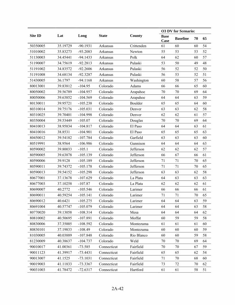
2A-42
Site ID Lat Long State County O3 DV for Scenario: Base Case
Baseline 70 65
50350005 35.19729 -90.1931 Arkansas Crittenden 61 60 60 54
51010002 35.83273 -93.2083 Arkansas Newton 55 53 53 52
51130003 34.45441 -94.1433 Arkansas Polk 64 62 60 57
51190007 34.75619 -92.2813 Arkansas Pulaski 53 50 49 48
51191002 34.83572 -92.2606 Arkansas Pulaski 56 52 52 50
51191008 34.68134 -92.3287 Arkansas Pulaski 56 53 52 51
51430005 36.1797 -94.1168 Arkansas Washington 60 58 57 56
80013001 39.83812 -104.95 Colorado Adams 66 66 65 60
80050002 39.56789 -104.957 Colorado Arapahoe 70 70 69 64
80050006 39.63852 -104.569 Colorado Arapahoe 64 64 63 59
80130011 39.95721 -105.238 Colorado Boulder 65 65 64 60
80310014 39.75176 -105.031 Colorado Denver 63 63 62 58
80310025 39.70401 -104.998 Colorado Denver 62 62 61 57
80350004 39.53449 -105.07 Colorado Douglas 70 70 69 64
80410013 38.95834 -104.817 Colorado El Paso 64 64 63 61
80410016 38.8531 -104.901 Colorado El Paso 65 65 65 63
80450012 39.54182 -107.784 Colorado Garfield 63 63 63 60
80519991 38.9564 -106.986 Colorado Gunnison 64 64 64 63
80590002 39.80033 -105.1 Colorado Jefferson 62 62 62 57
80590005 39.63878 -105.139 Colorado Jefferson 66 67 66 61
80590006 39.9128 -105.189 Colorado Jefferson 71 71 70 65
80590011 39.74372 -105.178 Colorado Jefferson 71 71 70 65
80590013 39.54152 -105.298 Colorado Jefferson 63 63 62 58
80677001 37.13678 -107.629 Colorado La Plata 64 63 63 63
80677003 37.10258 -107.87 Colorado La Plata 62 62 62 61
80690007 40.2772 -105.546 Colorado Larimer 66 66 66 61
80690011 40.59254 -105.141 Colorado Larimer 71 71 70 65
80690012 40.6421 -105.275 Colorado Larimer 64 64 63 59
80691004 40.57747 -105.079 Colorado Larimer 64 64 63 58
80770020 39.13058 -108.314 Colorado Mesa 64 64 64 62
80810002 40.50695 -107.891 Colorado Moffat 60 59 59 58
80830006 37.35005 -108.592 Colorado Montezuma 61 61 61 60
80830101 37.19833 -108.49 Colorado Montezuma 60 60 60 59
81030005 40.03889 -107.848 Colorado Rio Blanco 60 60 59 58
81230009 40.38637 -104.737 Colorado Weld 70 70 69 64
90010017 41.00361 -73.585 Connecticut Fairfield 70 70 67 59
90011123 41.39917 -73.4431 Connecticut Fairfield 65 65 62 54
90013007 41.1525 -73.1031 Connecticut Fairfield 71 70 68 60
90019003 41.11833 -73.3367 Connecticut Fairfield 73 72 70 62
90031003 41.78472 -72.6317 Connecticut Hartford 61 61 58 51
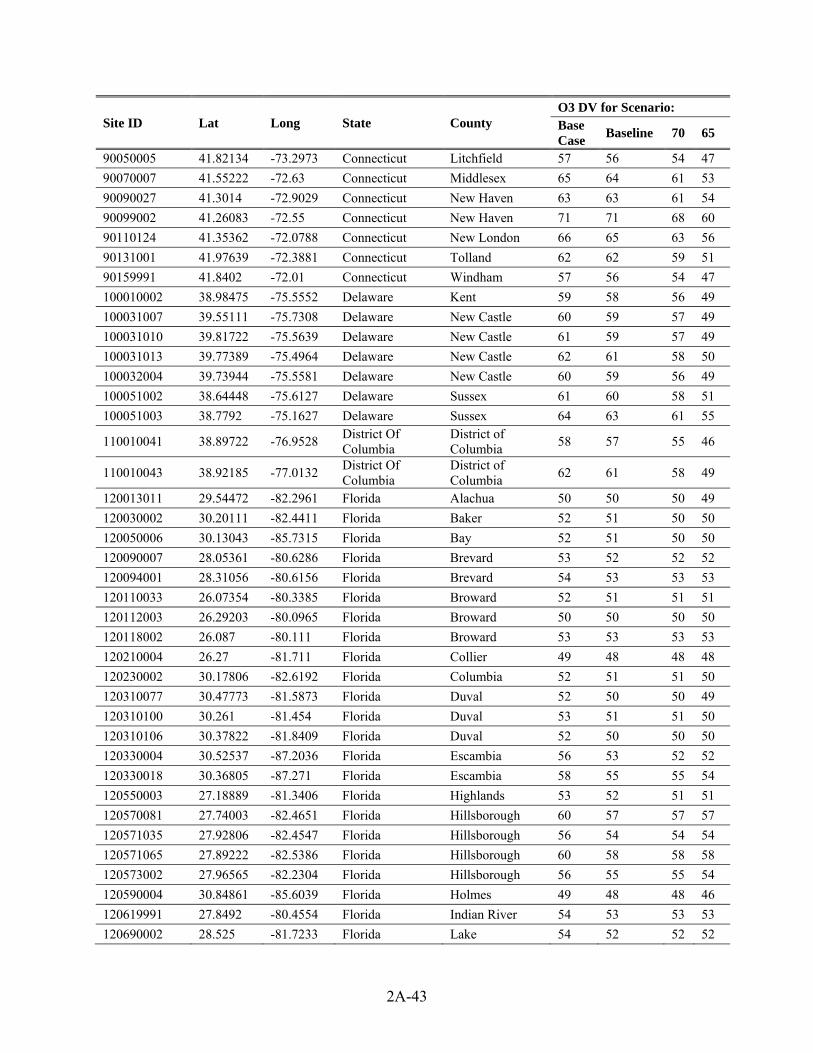
2A-43
Site ID Lat Long State County O3 DV for Scenario: Base Case
Baseline 70 65
90050005 41.82134 -73.2973 Connecticut Litchfield 57 56 54 47
90070007 41.55222 -72.63 Connecticut Middlesex 65 64 61 53
90090027 41.3014 -72.9029 Connecticut New Haven 63 63 61 54
90099002 41.26083 -72.55 Connecticut New Haven 71 71 68 60
90110124 41.35362 -72.0788 Connecticut New London 66 65 63 56
90131001 41.97639 -72.3881 Connecticut Tolland 62 62 59 51
90159991 41.8402 -72.01 Connecticut Windham 57 56 54 47
100010002 38.98475 -75.5552 Delaware Kent 59 58 56 49
100031007 39.55111 -75.7308 Delaware New Castle 60 59 57 49
100031010 39.81722 -75.5639 Delaware New Castle 61 59 57 49
100031013 39.77389 -75.4964 Delaware New Castle 62 61 58 50
100032004 39.73944 -75.5581 Delaware New Castle 60 59 56 49
100051002 38.64448 -75.6127 Delaware Sussex 61 60 58 51
100051003 38.7792 -75.1627 Delaware Sussex 64 63 61 55
110010041 38.89722 -76.9528 District Of Columbia
District of Columbia
58 57 55 46
110010043 38.92185 -77.0132 District Of Columbia
District of Columbia
62 61 58 49
120013011 29.54472 -82.2961 Florida Alachua 50 50 50 49
120030002 30.20111 -82.4411 Florida Baker 52 51 50 50
120050006 30.13043 -85.7315 Florida Bay 52 51 50 50
120090007 28.05361 -80.6286 Florida Brevard 53 52 52 52
120094001 28.31056 -80.6156 Florida Brevard 54 53 53 53
120110033 26.07354 -80.3385 Florida Broward 52 51 51 51
120112003 26.29203 -80.0965 Florida Broward 50 50 50 50
120118002 26.087 -80.111 Florida Broward 53 53 53 53
120210004 26.27 -81.711 Florida Collier 49 48 48 48
120230002 30.17806 -82.6192 Florida Columbia 52 51 51 50
120310077 30.47773 -81.5873 Florida Duval 52 50 50 49
120310100 30.261 -81.454 Florida Duval 53 51 51 50
120310106 30.37822 -81.8409 Florida Duval 52 50 50 50
120330004 30.52537 -87.2036 Florida Escambia 56 53 52 52
120330018 30.36805 -87.271 Florida Escambia 58 55 55 54
120550003 27.18889 -81.3406 Florida Highlands 53 52 51 51
120570081 27.74003 -82.4651 Florida Hillsborough 60 57 57 57
120571035 27.92806 -82.4547 Florida Hillsborough 56 54 54 54
120571065 27.89222 -82.5386 Florida Hillsborough 60 58 58 58
120573002 27.96565 -82.2304 Florida Hillsborough 56 55 55 54
120590004 30.84861 -85.6039 Florida Holmes 49 48 48 46
120619991 27.8492 -80.4554 Florida Indian River 54 53 53 53
120690002 28.525 -81.7233 Florida Lake 54 52 52 52
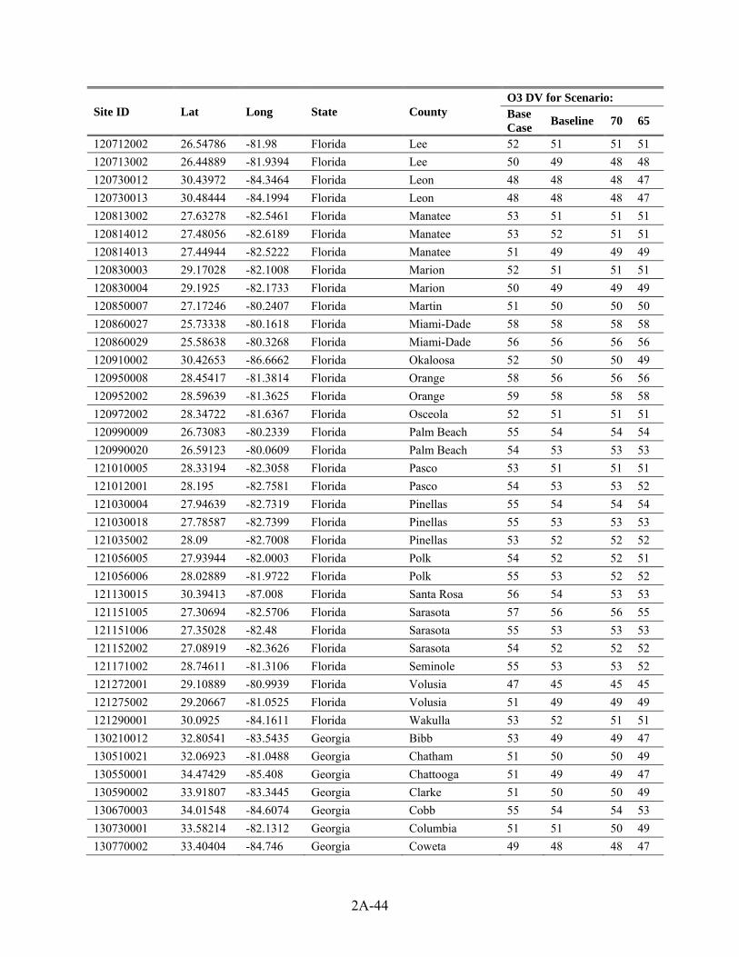
2A-44
Site ID Lat Long State County O3 DV for Scenario: Base Case
Baseline 70 65
120712002 26.54786 -81.98 Florida Lee 52 51 51 51
120713002 26.44889 -81.9394 Florida Lee 50 49 48 48
120730012 30.43972 -84.3464 Florida Leon 48 48 48 47
120730013 30.48444 -84.1994 Florida Leon 48 48 48 47
120813002 27.63278 -82.5461 Florida Manatee 53 51 51 51
120814012 27.48056 -82.6189 Florida Manatee 53 52 51 51
120814013 27.44944 -82.5222 Florida Manatee 51 49 49 49
120830003 29.17028 -82.1008 Florida Marion 52 51 51 51
120830004 29.1925 -82.1733 Florida Marion 50 49 49 49
120850007 27.17246 -80.2407 Florida Martin 51 50 50 50
120860027 25.73338 -80.1618 Florida Miami-Dade 58 58 58 58
120860029 25.58638 -80.3268 Florida Miami-Dade 56 56 56 56
120910002 30.42653 -86.6662 Florida Okaloosa 52 50 50 49
120950008 28.45417 -81.3814 Florida Orange 58 56 56 56
120952002 28.59639 -81.3625 Florida Orange 59 58 58 58
120972002 28.34722 -81.6367 Florida Osceola 52 51 51 51
120990009 26.73083 -80.2339 Florida Palm Beach 55 54 54 54
120990020 26.59123 -80.0609 Florida Palm Beach 54 53 53 53
121010005 28.33194 -82.3058 Florida Pasco 53 51 51 51
121012001 28.195 -82.7581 Florida Pasco 54 53 53 52
121030004 27.94639 -82.7319 Florida Pinellas 55 54 54 54
121030018 27.78587 -82.7399 Florida Pinellas 55 53 53 53
121035002 28.09 -82.7008 Florida Pinellas 53 52 52 52
121056005 27.93944 -82.0003 Florida Polk 54 52 52 51
121056006 28.02889 -81.9722 Florida Polk 55 53 52 52
121130015 30.39413 -87.008 Florida Santa Rosa 56 54 53 53
121151005 27.30694 -82.5706 Florida Sarasota 57 56 56 55
121151006 27.35028 -82.48 Florida Sarasota 55 53 53 53
121152002 27.08919 -82.3626 Florida Sarasota 54 52 52 52
121171002 28.74611 -81.3106 Florida Seminole 55 53 53 52
121272001 29.10889 -80.9939 Florida Volusia 47 45 45 45
121275002 29.20667 -81.0525 Florida Volusia 51 49 49 49
121290001 30.0925 -84.1611 Florida Wakulla 53 52 51 51
130210012 32.80541 -83.5435 Georgia Bibb 53 49 49 47
130510021 32.06923 -81.0488 Georgia Chatham 51 50 50 49
130550001 34.47429 -85.408 Georgia Chattooga 51 49 49 47
130590002 33.91807 -83.3445 Georgia Clarke 51 50 50 49
130670003 34.01548 -84.6074 Georgia Cobb 55 54 54 53
130730001 33.58214 -82.1312 Georgia Columbia 51 51 50 49
130770002 33.40404 -84.746 Georgia Coweta 49 48 48 47

2A-45
Site ID Lat Long State County O3 DV for Scenario: Base Case
Baseline 70 65
130850001 34.37632 -84.0598 Georgia Dawson 49 48 48 47
130890002 33.68797 -84.2905 Georgia DeKalb 56 55 55 54
130970004 33.74366 -84.7792 Georgia Douglas 52 51 51 50
131210055 33.72019 -84.3571 Georgia Fulton 59 58 58 57
131270006 31.16974 -81.4959 Georgia Glynn 48 47 47 47
131350002 33.96127 -84.069 Georgia Gwinnett 55 54 54 53
131510002 33.43358 -84.1617 Georgia Henry 59 58 58 57
132130003 34.7852 -84.6264 Georgia Murray 52 51 51 48
132150008 32.5213 -84.9448 Georgia Muscogee 50 50 49 49
132230003 33.9285 -85.0453 Georgia Paulding 53 51 51 49
132319991 33.1787 -84.4052 Georgia Pike 52 51 51 50
132450091 33.43335 -82.0222 Georgia Richmond 53 52 51 50
132470001 33.59108 -84.0653 Georgia Rockdale 55 54 54 53
132611001 31.9543 -84.0811 Georgia Sumter 53 52 52 51
160010010 43.6007 -116.348 Idaho Ada 60 59 59 59
160010017 43.5776 -116.178 Idaho Ada 60 60 60 60
160010019 43.63459 -116.234 Idaho Ada 54 53 53 53
160550003 47.78891 -116.805 Idaho Kootenai 47 47 47 47
170010007 39.91541 -91.3359 Illinois Adams 57 56 55 54
170190007 40.24491 -88.1885 Illinois Champaign 60 59 59 56
170191001 40.05224 -88.3725 Illinois Champaign 61 60 60 57
170230001 39.21086 -87.6683 Illinois Clark 58 58 58 53
170310001 41.67099 -87.7325 Illinois Cook 64 63 63 58
170310032 41.75583 -87.5454 Illinois Cook 57 57 57 57
170310064 41.79079 -87.6016 Illinois Cook 53 52 52 52
170310076 41.7514 -87.7135 Illinois Cook 63 63 62 58
170311003 41.98433 -87.792 Illinois Cook 49 49 49 50
170311601 41.66812 -87.9906 Illinois Cook 62 62 61 57
170314002 41.85524 -87.7525 Illinois Cook 52 51 51 51
170314007 42.06029 -87.8632 Illinois Cook 48 48 48 49
170314201 42.14 -87.7992 Illinois Cook 56 55 55 57
170317002 42.06186 -87.6742 Illinois Cook 54 54 54 56
170436001 41.81305 -88.0728 Illinois DuPage 58 58 57 53
170491001 39.06716 -88.5489 Illinois Effingham 58 58 57 54
170650002 38.08216 -88.6249 Illinois Hamilton 64 65 65 61
170831001 39.11054 -90.3241 Illinois Jersey 61 60 60 59
170859991 42.2869 -89.9997 Illinois Jo Daviess 58 57 56 55
170890005 42.04915 -88.273 Illinois Kane 63 62 62 58
170971007 42.46757 -87.81 Illinois Lake 57 57 57 58
171110001 42.22144 -88.2422 Illinois McHenry 61 60 60 55
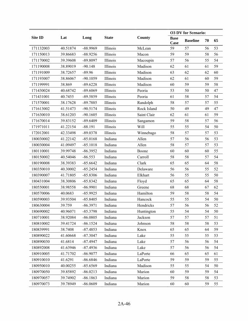
2A-46
Site ID Lat Long State County O3 DV for Scenario: Base Case
Baseline 70 65
171132003 40.51874 -88.9969 Illinois McLean 59 57 56 53
171150013 39.86683 -88.9256 Illinois Macon 59 59 58 56
171170002 39.39608 -89.8097 Illinois Macoupin 57 56 55 54
171190008 38.89019 -90.148 Illinois Madison 62 61 61 59
171191009 38.72657 -89.96 Illinois Madison 63 62 62 60
171193007 38.86067 -90.1059 Illinois Madison 62 61 60 59
171199991 38.869 -89.6228 Illinois Madison 60 59 59 58
171430024 40.68742 -89.6069 Illinois Peoria 53 50 50 47
171431001 40.7455 -89.5859 Illinois Peoria 61 58 57 54
171570001 38.17628 -89.7885 Illinois Randolph 58 57 57 55
171613002 41.51473 -90.5174 Illinois Rock Island 50 49 49 47
171630010 38.61203 -90.1605 Illinois Saint Clair 62 61 61 59
171670014 39.83152 -89.6409 Illinois Sangamon 59 58 57 56
171971011 41.22154 -88.191 Illinois Will 55 55 54 50
172012001 42.33498 -89.0378 Illinois Winnebago 58 57 57 53
180030002 41.22142 -85.0168 Indiana Allen 57 56 56 53
180030004 41.09497 -85.1018 Indiana Allen 58 57 57 53
180110001 39.99748 -86.3952 Indiana Boone 60 60 60 55
180150002 40.54046 -86.553 Indiana Carroll 58 58 57 54
180190008 38.39383 -85.6642 Indiana Clark 65 65 64 58
180350010 40.30002 -85.2454 Indiana Delaware 56 56 55 52
180390007 41.71805 -85.8306 Indiana Elkhart 56 55 55 50
180431004 38.30806 -85.8342 Indiana Floyd 65 65 64 58
180550001 38.98558 -86.9901 Indiana Greene 68 68 67 62
180570006 40.0683 -85.9925 Indiana Hamilton 59 58 58 54
180590003 39.93504 -85.8405 Indiana Hancock 55 55 54 50
180630004 39.759 -86.3971 Indiana Hendricks 57 56 56 52
180690002 40.96071 -85.3798 Indiana Huntington 55 54 54 50
180710001 38.92084 -86.0805 Indiana Jackson 57 57 57 51
180810002 39.41724 -86.1524 Indiana Johnson 58 58 58 53
180839991 38.7408 -87.4853 Indiana Knox 65 65 64 59
180890022 41.60668 -87.3047 Indiana Lake 55 55 55 53
180890030 41.6814 -87.4947 Indiana Lake 57 56 56 54
180892008 41.63946 -87.4936 Indiana Lake 57 56 56 54
180910005 41.71702 -86.9077 Indiana LaPorte 66 65 65 61
180910010 41.6291 -86.6846 Indiana LaPorte 59 59 59 55
180950010 40.00255 -85.6569 Indiana Madison 55 55 54 50
180970050 39.85892 -86.0213 Indiana Marion 60 59 59 54
180970057 39.74902 -86.1863 Indiana Marion 59 58 58 53
180970073 39.78949 -86.0609 Indiana Marion 60 60 59 55
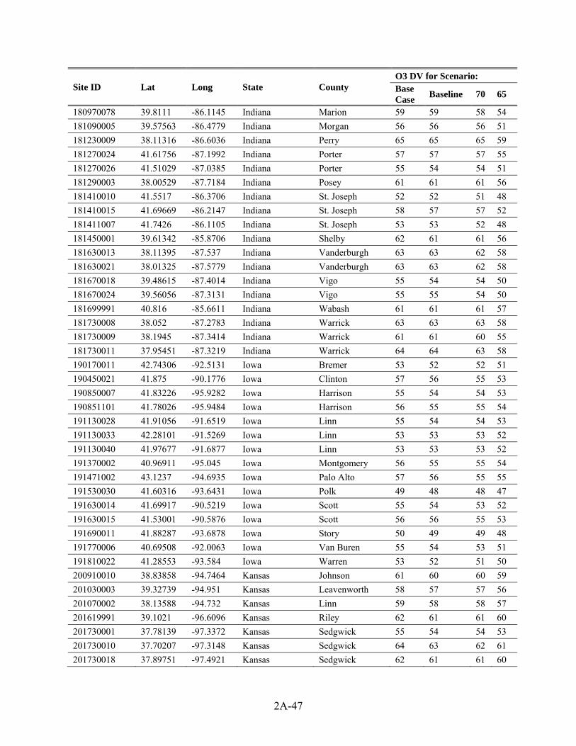
2A-47
Site ID Lat Long State County O3 DV for Scenario: Base Case
Baseline 70 65
180970078 39.8111 -86.1145 Indiana Marion 59 59 58 54
181090005 39.57563 -86.4779 Indiana Morgan 56 56 56 51
181230009 38.11316 -86.6036 Indiana Perry 65 65 65 59
181270024 41.61756 -87.1992 Indiana Porter 57 57 57 55
181270026 41.51029 -87.0385 Indiana Porter 55 54 54 51
181290003 38.00529 -87.7184 Indiana Posey 61 61 61 56
181410010 41.5517 -86.3706 Indiana St. Joseph 52 52 51 48
181410015 41.69669 -86.2147 Indiana St. Joseph 58 57 57 52
181411007 41.7426 -86.1105 Indiana St. Joseph 53 53 52 48
181450001 39.61342 -85.8706 Indiana Shelby 62 61 61 56
181630013 38.11395 -87.537 Indiana Vanderburgh 63 63 62 58
181630021 38.01325 -87.5779 Indiana Vanderburgh 63 63 62 58
181670018 39.48615 -87.4014 Indiana Vigo 55 54 54 50
181670024 39.56056 -87.3131 Indiana Vigo 55 55 54 50
181699991 40.816 -85.6611 Indiana Wabash 61 61 61 57
181730008 38.052 -87.2783 Indiana Warrick 63 63 63 58
181730009 38.1945 -87.3414 Indiana Warrick 61 61 60 55
181730011 37.95451 -87.3219 Indiana Warrick 64 64 63 58
190170011 42.74306 -92.5131 Iowa Bremer 53 52 52 51
190450021 41.875 -90.1776 Iowa Clinton 57 56 55 53
190850007 41.83226 -95.9282 Iowa Harrison 55 54 54 53
190851101 41.78026 -95.9484 Iowa Harrison 56 55 55 54
191130028 41.91056 -91.6519 Iowa Linn 55 54 54 53
191130033 42.28101 -91.5269 Iowa Linn 53 53 53 52
191130040 41.97677 -91.6877 Iowa Linn 53 53 53 52
191370002 40.96911 -95.045 Iowa Montgomery 56 55 55 54
191471002 43.1237 -94.6935 Iowa Palo Alto 57 56 55 55
191530030 41.60316 -93.6431 Iowa Polk 49 48 48 47
191630014 41.69917 -90.5219 Iowa Scott 55 54 53 52
191630015 41.53001 -90.5876 Iowa Scott 56 56 55 53
191690011 41.88287 -93.6878 Iowa Story 50 49 49 48
191770006 40.69508 -92.0063 Iowa Van Buren 55 54 53 51
191810022 41.28553 -93.584 Iowa Warren 53 52 51 50
200910010 38.83858 -94.7464 Kansas Johnson 61 60 60 59
201030003 39.32739 -94.951 Kansas Leavenworth 58 57 57 56
201070002 38.13588 -94.732 Kansas Linn 59 58 58 57
201619991 39.1021 -96.6096 Kansas Riley 62 61 61 60
201730001 37.78139 -97.3372 Kansas Sedgwick 55 54 54 53
201730010 37.70207 -97.3148 Kansas Sedgwick 64 63 62 61
201730018 37.89751 -97.4921 Kansas Sedgwick 62 61 61 60

2A-48
Site ID Lat Long State County O3 DV for Scenario: Base Case
Baseline 70 65
201770013 39.02427 -95.7113 Kansas Shawnee 62 61 61 61
201910002 37.47689 -97.3664 Kansas Sumner 65 64 64 63
201950001 38.77008 -99.7634 Kansas Trego 65 65 65 64
202090021 39.11722 -94.6356 Kansas Wyandotte 55 54 54 53
210130002 36.60843 -83.7369 Kentucky Bell 50 49 49 45
210150003 38.91833 -84.8526 Kentucky Boone 59 58 57 51
210190017 38.45934 -82.6404 Kentucky Boyd 58 58 57 50
210290006 37.98629 -85.7119 Kentucky Bullitt 62 62 61 56
210373002 39.02188 -84.4745 Kentucky Campbell 66 66 65 58
210430500 38.23887 -82.9881 Kentucky Carter 56 56 55 49
210470006 36.91171 -87.3233 Kentucky Christian 53 53 52 49
210590005 37.78078 -87.0753 Kentucky Daviess 67 67 67 61
210610501 37.13194 -86.1478 Kentucky Edmonson 57 57 57 53
210670012 38.06503 -84.4976 Kentucky Fayette 58 58 58 52
210890007 38.54814 -82.7312 Kentucky Greenup 59 59 58 51
210910012 37.93829 -86.8972 Kentucky Hancock 66 66 66 60
210930006 37.70561 -85.8526 Kentucky Hardin 59 59 58 53
211010014 37.8712 -87.4638 Kentucky Henderson 68 68 68 63
211110027 38.13784 -85.5765 Kentucky Jefferson 66 65 65 59
211110051 38.06091 -85.898 Kentucky Jefferson 68 68 67 61
211110067 38.22876 -85.6545 Kentucky Jefferson 71 71 70 63
211130001 37.89147 -84.5883 Kentucky Jessamine 56 57 57 52
211390003 37.15539 -88.394 Kentucky Livingston 61 65 65 60
211451024 37.05822 -88.5725 Kentucky McCracken 64 69 68 64
211759991 37.9214 -83.0662 Kentucky Morgan 57 56 56 49
211850004 38.4002 -85.4443 Kentucky Oldham 68 68 67 60
211930003 37.28329 -83.2093 Kentucky Perry 56 56 55 49
211950002 37.4826 -82.5353 Kentucky Pike 56 56 55 48
211990003 37.09798 -84.6115 Kentucky Pulaski 51 51 50 46
212130004 36.70861 -86.5663 Kentucky Simpson 53 53 53 48
212218001 36.78389 -87.8519 Kentucky Trigg 56 57 56 51
212219991 36.7841 -87.8499 Kentucky Trigg 57 58 57 52
212270008 37.03544 -86.2506 Kentucky Warren 51 50 50 46
212299991 37.7046 -85.0485 Kentucky Washington 57 57 57 52
220050004 30.23389 -90.9683 Louisiana Ascension 63 62 62 61
220150008 32.53626 -93.7489 Louisiana Bossier 66 64 62 59
220170001 32.67639 -93.8597 Louisiana Caddo 64 62 60 56
220190002 30.14333 -93.3719 Louisiana Calcasieu 66 66 65 64
220190008 30.26167 -93.2842 Louisiana Calcasieu 60 60 59 58
220190009 30.22778 -93.5783 Louisiana Calcasieu 63 62 60 57

2A-49
Site ID Lat Long State County O3 DV for Scenario: Base Case
Baseline 70 65
220330003 30.41976 -91.182 Louisiana East Baton Rouge
67 67 67 65
220330009 30.46198 -91.1792 Louisiana East Baton Rouge
64 63 63 62
220330013 30.70092 -91.0561 Louisiana East Baton Rouge
60 59 59 58
220470009 30.22056 -91.3161 Louisiana Iberville 62 62 61 60
220470012 30.20699 -91.1299 Louisiana Iberville 65 65 64 63
220511001 30.04357 -90.2751 Louisiana Jefferson 64 64 63 63
220550007 30.2175 -92.0514 Louisiana Lafayette 60 60 59 58
220570004 29.76389 -90.7652 Louisiana Lafourche 62 61 61 60
220630002 30.3125 -90.8125 Louisiana Livingston 62 62 62 61
220710012 29.99444 -90.1028 Louisiana Orleans 60 59 58 58
220730004 32.50971 -92.0461 Louisiana Ouachita 55 55 55 54
220770001 30.68174 -91.3662 Louisiana Pointe Coupee 63 62 62 61
220870004 29.93961 -89.9239 Louisiana St. Bernard 59 58 58 57
220890003 29.98417 -90.4106 Louisiana St. Charles 61 60 60 59
220930002 29.99444 -90.82 Louisiana St. James 58 58 58 57
220950002 30.05833 -90.6083 Louisiana St. John the Baptist
63 62 62 61
221030002 30.4293 -90.1997 Louisiana St. Tammany 63 62 62 61
221210001 30.50064 -91.2136 Louisiana West Baton Rouge
59 59 59 58
230010014 43.97462 -70.1246 Maine Androscoggin 50 49 48 44
230052003 43.56104 -70.2073 Maine Cumberland 57 57 55 50
230090102 44.3517 -68.227 Maine Hancock 58 57 56 52
230090103 44.37705 -68.2609 Maine Hancock 55 54 53 49
230112005 44.23062 -69.785 Maine Kennebec 50 50 49 45
230130004 43.91796 -69.2606 Maine Knox 55 55 53 49
230173001 44.25092 -70.8606 Maine Oxford 46 45 45 42
230194008 44.73598 -68.6708 Maine Penobscot 47 46 45 42
230230006 44.005 -69.8278 Maine Sagadahoc 49 49 47 43
230290019 44.53191 -67.5959 Maine Washington 49 49 48 44
230290032 44.96363 -67.0607 Maine Washington 46 46 45 42
230310038 43.65676 -70.6291 Maine York 49 48 47 43
230310040 43.58889 -70.8773 Maine York 52 51 50 46
230312002 43.34317 -70.471 Maine York 60 59 57 52
240030014 38.9025 -76.6531 Maryland Anne Arundel 64 63 61 51
240051007 39.46202 -76.6313 Maryland Baltimore 65 63 61 53
240053001 39.31083 -76.4744 Maryland Baltimore 67 66 63 53
240090011 38.53672 -76.6172 Maryland Calvert 63 63 60 51
240130001 39.44417 -77.0417 Maryland Carroll 61 60 59 51

2A-50
Site ID Lat Long State County O3 DV for Scenario: Base Case
Baseline 70 65
240150003 39.70111 -75.86 Maryland Cecil 66 65 62 54
240170010 38.50417 -76.8119 Maryland Charles 61 60 58 50
240199991 38.445 -76.1114 Maryland Dorchester 61 60 58 52
240210037 39.42276 -77.3752 Maryland Frederick 62 62 60 52
240230002 39.70595 -79.012 Maryland Garrett 59 59 58 52
240251001 39.41 -76.2967 Maryland Harford 74 73 70 59
240259001 39.56333 -76.2039 Maryland Harford 63 61 59 49
240290002 39.3052 -75.7972 Maryland Kent 62 61 58 50
240313001 39.11444 -77.1069 Maryland Montgomery 60 59 57 49
240330030 39.05528 -76.8783 Maryland Prince George's 61 60 58 49
240338003 38.81194 -76.7442 Maryland Prince George's 63 62 60 50
240339991 39.0284 -76.8171 Maryland Prince George's 62 61 58 50
240430009 39.56558 -77.7216 Maryland Washington 60 59 58 52
245100054 39.32889 -76.5525 Maryland Baltimore (City) 62 62 59 50
250010002 41.9758 -70.0236 Massachusetts Barnstable 59 59 57 51
250034002 42.63668 -73.1674 Massachusetts Berkshire 57 57 55 50
250051002 41.63328 -70.8792 Massachusetts Bristol 59 59 57 50
250070001 41.33047 -70.7852 Massachusetts Dukes 64 64 62 54
250092006 42.47464 -70.9708 Massachusetts Essex 58 57 56 52
250094005 42.81441 -70.8178 Massachusetts Essex 57 56 55 50
250095005 42.77084 -71.1023 Massachusetts Essex 56 56 54 49
250130008 42.19438 -72.5551 Massachusetts Hampden 59 59 56 49
250150103 42.40058 -72.5231 Massachusetts Hampshire 52 52 50 44
250154002 42.29849 -72.3341 Massachusetts Hampshire 57 56 54 47
250170009 42.62668 -71.3621 Massachusetts Middlesex 55 54 52 46
250171102 42.41357 -71.4828 Massachusetts Middlesex 54 53 51 45
250213003 42.21177 -71.114 Massachusetts Norfolk 59 59 57 52
250250041 42.31737 -70.9684 Massachusetts Suffolk 56 55 54 50
250250042 42.3295 -71.0826 Massachusetts Suffolk 49 49 48 44
250270015 42.27432 -71.8755 Massachusetts Worcester 55 55 53 47
250270024 42.0997 -71.6194 Massachusetts Worcester 55 54 53 47
260050003 42.76779 -86.1486 Michigan Allegan 70 69 69 63
260190003 44.61694 -86.1094 Michigan Benzie 62 61 61 56
260210014 42.19779 -86.3097 Michigan Berrien 68 68 67 62
260270003 41.89557 -86.0016 Michigan Cass 63 62 62 57
260370001 42.79834 -84.3938 Michigan Clinton 57 56 55 51
260490021 43.04722 -83.6702 Michigan Genesee 61 60 60 56
260492001 43.16834 -83.4615 Michigan Genesee 60 60 59 55
260630007 43.83639 -82.6429 Michigan Huron 61 61 60 57
260650012 42.73862 -84.5346 Michigan Ingham 57 56 56 52

2A-51
Site ID Lat Long State County O3 DV for Scenario: Base Case
Baseline 70 65
260770008 42.27807 -85.5419 Michigan Kalamazoo 61 60 59 55
260810020 42.98417 -85.6713 Michigan Kent 60 59 59 54
260810022 43.17667 -85.4166 Michigan Kent 59 58 58 53
260910007 41.99557 -83.9466 Michigan Lenawee 60 60 59 55
260990009 42.73139 -82.7935 Michigan Macomb 67 67 66 62
260991003 42.51334 -83.006 Michigan Macomb 69 68 68 63
261010922 44.307 -86.2426 Michigan Manistee 61 60 60 55
261050007 43.95333 -86.2944 Michigan Mason 62 61 60 56
261130001 44.31056 -84.8919 Michigan Missaukee 58 57 57 53
261210039 43.27806 -86.3111 Michigan Muskegon 66 66 65 60
261250001 42.46306 -83.1832 Michigan Oakland 66 65 65 60
261390005 42.89445 -85.8527 Michigan Ottawa 63 62 62 57
261470005 42.95334 -82.4562 Michigan St. Clair 65 65 65 60
261530001 46.28888 -85.9502 Michigan Schoolcraft 60 60 59 55
261579991 43.6138 -83.3591 Michigan Tuscola 58 57 57 52
261610008 42.24057 -83.5996 Michigan Washtenaw 62 62 62 58
261619991 42.4165 -83.902 Michigan Washtenaw 60 60 59 55
261630001 42.22862 -83.2082 Michigan Wayne 61 61 61 57
261630019 42.43084 -83.0001 Michigan Wayne 70 70 69 65
261659991 44.1809 -85.739 Michigan Wexford 56 55 55 51
270031001 45.40184 -93.2031 Minnesota Anoka 53 53 53 52
270031002 45.13768 -93.2076 Minnesota Anoka 57 56 56 56
270353204 46.39674 -94.1303 Minnesota Crow Wing 51 49 49 49
270495302 44.47375 -93.0126 Minnesota Goodhue 53 53 53 52
270953051 46.2053 -93.7595 Minnesota Mille Lacs 48 47 47 47
271095008 43.99691 -92.4504 Minnesota Olmsted 53 53 53 52
271377550 46.81826 -92.0894 Minnesota Saint Louis 42 41 41 40
271390505 44.79144 -93.5125 Minnesota Scott 54 53 53 53
271453052 45.54984 -94.1335 Minnesota Stearns 53 50 50 50
271636015 45.11728 -92.8553 Minnesota Washington 52 52 51 51
271713201 45.20916 -93.6692 Minnesota Wright 55 52 52 52
280010004 31.56075 -91.3904 Mississippi Adams 55 54 54 53
280110001 33.74606 -90.723 Mississippi Bolivar 61 60 60 59
280330002 34.82166 -89.9878 Mississippi DeSoto 57 55 55 51
280450003 30.30083 -89.3959 Mississippi Hancock 53 50 50 49
280470008 30.39037 -89.0498 Mississippi Harrison 56 51 51 50
280490010 32.38573 -90.1412 Mississippi Hinds 49 48 48 47
280590006 30.37829 -88.5339 Mississippi Jackson 59 58 58 57
280750003 32.36457 -88.7315 Mississippi Lauderdale 50 49 49 47
280810005 34.26492 -88.7662 Mississippi Lee 51 50 50 48

2A-52
Site ID Lat Long State County O3 DV for Scenario: Base Case
Baseline 70 65
281619991 34.0026 -89.799 Mississippi Yalobusha 52 51 51 49
290030001 39.9544 -94.849 Missouri Andrew 60 59 58 57
290190011 39.0786 -92.3152 Missouri Boone 56 56 56 55
290270002 38.70608 -92.0931 Missouri Callaway 56 55 55 54
290370003 38.75976 -94.58 Missouri Cass 57 57 57 56
290390001 37.69 -94.035 Missouri Cedar 61 60 59 57
290470003 39.40745 -94.2654 Missouri Clay 63 62 62 61
290470005 39.30309 -94.3766 Missouri Clay 62 61 61 60
290470006 39.33191 -94.5808 Missouri Clay 64 63 63 62
290490001 39.5306 -94.556 Missouri Clinton 64 63 63 62
290770036 37.25614 -93.2999 Missouri Greene 56 55 55 54
290770042 37.31951 -93.2046 Missouri Greene 58 57 57 56
290970004 37.2385 -94.4247 Missouri Jasper 65 62 61 58
290990019 38.44863 -90.3985 Missouri Jefferson 64 63 63 62
291130003 39.0447 -90.8647 Missouri Lincoln 63 62 62 61
291370001 39.47514 -91.7891 Missouri Monroe 58 57 57 55
291570001 37.70264 -89.6986 Missouri Perry 62 62 62 59
291831002 38.87255 -90.2265 Missouri Saint Charles 66 65 65 64
291831004 38.8994 -90.4492 Missouri Saint Charles 65 64 64 62
291860005 37.90084 -90.4239 Missouri Sainte Genevieve
61 60 60 59
291890005 38.4902 -90.7052 Missouri Saint Louis 59 59 58 57
291890014 38.7109 -90.4759 Missouri Saint Louis 65 64 64 63
292130004 36.70773 -93.222 Missouri Taney 59 57 57 55
295100085 38.6565 -90.1986 Missouri St. Louis City 63 63 62 61
300870001 45.36615 -106.49 Montana Rosebud 53 52 52 52
310550019 41.24749 -95.9731 Nebraska Douglas 58 57 57 57
310550028 41.20796 -95.9459 Nebraska Douglas 51 50 50 50
310550035 41.30676 -95.961 Nebraska Douglas 54 53 53 53
311090016 40.98472 -96.6772 Nebraska Lancaster 47 47 46 46
320010002 39.47247 -118.784 Nevada Churchill 52 52 52 52
320030022 36.39101 -114.907 Nevada Clark 63 62 62 60
320030023 36.80791 -114.061 Nevada Clark 57 57 57 56
320030043 36.10637 -115.253 Nevada Clark 69 69 69 65
320030071 36.16975 -115.263 Nevada Clark 69 69 69 65
320030073 36.17342 -115.333 Nevada Clark 68 68 68 65
320030075 36.27058 -115.238 Nevada Clark 68 67 67 64
320030538 36.14296 -115.056 Nevada Clark 63 63 63 60
320030540 36.1419 -115.079 Nevada Clark 63 63 63 60
320030601 35.97813 -114.846 Nevada Clark 65 65 65 63
320031019 35.78567 -115.357 Nevada Clark 67 67 67 65

2A-53
Site ID Lat Long State County O3 DV for Scenario: Base Case
Baseline 70 65
320032002 36.19126 -115.123 Nevada Clark 63 63 63 60
320190006 39.60279 -119.248 Nevada Lyon 60 60 60 60
320310016 39.52508 -119.808 Nevada Washoe 59 58 58 58
320310020 39.46922 -119.775 Nevada Washoe 59 59 59 59
320310025 39.39984 -119.74 Nevada Washoe 59 59 59 58
320311005 39.54092 -119.747 Nevada Washoe 59 59 59 59
320312002 39.25041 -119.957 Nevada Washoe 53 53 53 53
320312009 39.64526 -119.84 Nevada Washoe 59 59 59 58
325100002 39.16725 -119.732 Nevada Carson City 59 59 59 59
330012004 43.56611 -71.4964 New Hampshire Belknap 51 51 50 46
330050007 42.93047 -72.2724 New Hampshire Cheshire 50 50 48 44
330074001 44.27017 -71.3038 New Hampshire Coos 58 57 57 54
330074002 44.30817 -71.2177 New Hampshire Coos 51 51 50 48
330090010 43.62961 -72.3096 New Hampshire Grafton 50 49 48 45
330111011 42.71866 -71.5224 New Hampshire Hillsborough 54 53 51 46
330115001 42.86175 -71.8784 New Hampshire Hillsborough 57 56 55 49
330131007 43.2185 -71.5145 New Hampshire Merrimack 52 52 50 46
330150014 43.07533 -70.748 New Hampshire Rockingham 54 53 52 47
330150016 43.04528 -70.7138 New Hampshire Rockingham 54 54 52 48
330150018 42.86254 -71.3802 New Hampshire Rockingham 55 55 53 47
340010006 39.46487 -74.4487 New Jersey Atlantic 60 59 57 50
340030006 40.87044 -73.992 New Jersey Bergen 64 63 61 53
340071001 39.68425 -74.8615 New Jersey Camden 68 67 64 55
340110007 39.42227 -75.0252 New Jersey Cumberland 59 57 55 47
340130003 40.72099 -74.1929 New Jersey Essex 65 64 61 53
340150002 39.80034 -75.2121 New Jersey Gloucester 69 68 65 56
340170006 40.67025 -74.1261 New Jersey Hudson 64 63 61 53
340190001 40.51526 -74.8067 New Jersey Hunterdon 63 62 60 52
340210005 40.28309 -74.7426 New Jersey Mercer 64 63 61 53
340219991 40.3125 -74.8729 New Jersey Mercer 62 61 59 51
340230011 40.46218 -74.4294 New Jersey Middlesex 66 65 62 53
340250005 40.27765 -74.0051 New Jersey Monmouth 67 65 63 54
340273001 40.78763 -74.6763 New Jersey Morris 63 62 60 52
340290006 40.06483 -74.4441 New Jersey Ocean 67 66 63 54
340315001 41.05862 -74.2555 New Jersey Passaic 62 61 59 52
340410007 40.92458 -75.0678 New Jersey Warren 52 52 50 44
350010023 35.1343 -106.585 New Mexico Bernalillo 58 58 58 57
350010024 35.0631 -106.579 New Mexico Bernalillo 59 59 59 58
350010027 35.1539 -106.697 New Mexico Bernalillo 62 62 62 61
350010029 35.01708 -106.657 New Mexico Bernalillo 59 59 59 58

2A-54
Site ID Lat Long State County O3 DV for Scenario: Base Case
Baseline 70 65
350010032 35.06407 -106.762 New Mexico Bernalillo 58 57 57 56
350011012 35.1852 -106.508 New Mexico Bernalillo 63 62 62 61
350011013 35.19324 -106.614 New Mexico Bernalillo 60 60 60 58
350130008 31.93056 -106.631 New Mexico Dona Ana 57 56 56 56
350130017 31.79583 -106.558 New Mexico Dona Ana 58 58 58 57
350130020 32.04111 -106.409 New Mexico Dona Ana 59 58 58 58
350130021 31.79611 -106.584 New Mexico Dona Ana 62 61 61 61
350130022 31.78778 -106.683 New Mexico Dona Ana 62 61 61 61
350130023 32.3175 -106.768 New Mexico Dona Ana 57 57 56 56
350171003 32.69194 -108.124 New Mexico Grant 61 61 61 60
350250008 32.72666 -103.123 New Mexico Lea 61 61 61 60
350290003 32.2558 -107.723 New Mexico Luna 58 57 57 56
350431001 35.29944 -106.548 New Mexico Sandoval 55 55 55 54
350439004 35.61528 -106.724 New Mexico Sandoval 58 58 58 58
350450009 36.74222 -107.977 New Mexico San Juan 57 57 57 56
350450018 36.80973 -107.652 New Mexico San Juan 62 62 62 61
350451005 36.79667 -108.473 New Mexico San Juan 56 55 55 54
350451233 36.8071 -108.695 New Mexico San Juan 56 55 55 54
350490021 35.61975 -106.08 New Mexico Santa Fe 60 59 59 59
350610008 34.8147 -106.74 New Mexico Valencia 58 58 58 56
360010012 42.68075 -73.7573 New York Albany 57 56 54 49
360050133 40.8679 -73.8781 New York Bronx 67 66 64 57
360130006 42.49963 -79.3188 New York Chautauqua 61 61 60 55
360130011 42.29071 -79.5896 New York Chautauqua 61 61 60 55
360150003 42.11096 -76.8022 New York Chemung 57 57 56 53
360270007 41.78555 -73.7414 New York Dutchess 58 57 55 48
360290002 42.99328 -78.7715 New York Erie 61 61 60 56
360310002 44.36608 -73.9031 New York Essex 57 57 56 54
360310003 44.39308 -73.8589 New York Essex 57 57 56 53
360410005 43.44957 -74.5163 New York Hamilton 57 56 55 52
360430005 43.68578 -74.9854 New York Herkimer 56 55 54 52
360450002 44.08747 -75.9732 New York Jefferson 62 62 61 60
360530006 42.73046 -75.7844 New York Madison 55 54 53 50
360551007 43.14618 -77.5482 New York Monroe 60 59 59 57
360610135 40.81976 -73.9483 New York New York 65 64 63 58
360631006 43.22386 -78.4789 New York Niagara 64 64 64 61
360650004 43.30268 -75.7198 New York Oneida 53 52 52 49
360671015 43.05235 -76.0592 New York Onondaga 59 59 58 56
360715001 41.52375 -74.2153 New York Orange 56 55 53 46
360750003 43.28428 -76.4632 New York Oswego 58 58 58 56

2A-55
Site ID Lat Long State County O3 DV for Scenario: Base Case
Baseline 70 65
360790005 41.45589 -73.7098 New York Putnam 57 56 54 47
360810124 40.73614 -73.8215 New York Queens 72 71 70 65
360830004 42.78189 -73.4636 New York Rensselaer 57 56 55 49
360850067 40.59664 -74.1253 New York Richmond 73 72 70 63
360870005 41.18208 -74.0282 New York Rockland 62 61 59 51
360910004 43.01209 -73.6489 New York Saratoga 56 55 54 49
360930003 42.79901 -73.9389 New York Schenectady 54 53 52 47
361010003 42.09142 -77.2098 New York Steuben 57 56 55 52
361030002 40.74529 -73.4192 New York Suffolk 74 73 70 62
361030004 40.96078 -72.7124 New York Suffolk 67 66 63 54
361030009 40.82799 -73.0575 New York Suffolk 71 70 68 59
361099991 42.4006 -76.6538 New York Tompkins 58 58 57 54
361111005 42.14403 -74.4943 New York Ulster 58 58 56 51
361173001 43.23086 -77.1714 New York Wayne 56 56 56 54
361192004 41.05192 -73.7637 New York Westchester 65 64 62 54
370030004 35.929 -81.1898 North Carolina Alexander 52 51 50 49
370110002 35.97222 -81.9331 North Carolina Avery 50 49 49 46
370119991 36.1058 -82.0454 North Carolina Avery 50 49 49 44
370210030 35.5001 -82.5999 North Carolina Buncombe 52 51 51 49
370270003 35.93583 -81.5303 North Carolina Caldwell 51 50 50 49
370319991 34.8848 -76.6203 North Carolina Carteret 51 50 50 48
370330001 36.30703 -79.4674 North Carolina Caswell 55 54 54 53
370370004 35.75722 -79.1597 North Carolina Chatham 49 48 47 46
370510008 35.15869 -78.728 North Carolina Cumberland 54 53 53 51
370511003 34.96889 -78.9625 North Carolina Cumberland 55 54 54 52
370590003 35.89707 -80.5573 North Carolina Davie 54 53 53 51
370630015 36.03294 -78.9054 North Carolina Durham 52 51 51 50
370650099 35.98833 -77.5828 North Carolina Edgecombe 56 54 54 52
370670022 36.11056 -80.2267 North Carolina Forsyth 58 57 57 55
370670028 36.20306 -80.2158 North Carolina Forsyth 54 53 53 51
370670030 36.026 -80.342 North Carolina Forsyth 56 55 55 53
370671008 36.05083 -80.1439 North Carolina Forsyth 55 55 55 53
370690001 36.09619 -78.4637 North Carolina Franklin 52 52 51 50
370750001 35.25793 -83.7956 North Carolina Graham 54 54 54 51
370770001 36.14111 -78.7681 North Carolina Granville 56 54 54 53
370810013 36.10071 -79.8105 North Carolina Guilford 57 56 56 55
370870008 35.50716 -82.9634 North Carolina Haywood 50 49 49 47
370870035 35.37917 -82.7925 North Carolina Haywood 55 54 54 52
370870036 35.59 -83.0775 North Carolina Haywood 55 54 54 52
370990005 35.52444 -83.2361 North Carolina Jackson 55 54 54 51

2A-56
Site ID Lat Long State County O3 DV for Scenario: Base Case
Baseline 70 65
371010002 35.59083 -78.4619 North Carolina Johnston 55 54 54 52
371070004 35.23146 -77.5688 North Carolina Lenoir 54 52 52 50
371090004 35.43856 -81.2768 North Carolina Lincoln 57 55 55 53
371139991 35.0608 -83.4306 North Carolina Macon 50 49 49 48
371170001 35.81069 -76.8978 North Carolina Martin 51 51 50 48
371190041 35.2401 -80.7857 North Carolina Mecklenburg 65 64 64 63
371191005 35.11316 -80.9195 North Carolina Mecklenburg 60 60 60 59
371191009 35.34722 -80.695 North Carolina Mecklenburg 62 61 61 60
371239991 35.2632 -79.8365 North Carolina Montgomery 50 49 49 48
371290002 34.36417 -77.8386 North Carolina New Hanover 50 49 49 48
371450003 36.30697 -79.092 North Carolina Person 63 56 56 54
371470006 35.63861 -77.3581 North Carolina Pitt 55 54 54 52
371570099 36.30889 -79.8592 North Carolina Rockingham 57 56 56 55
371590021 35.55187 -80.395 North Carolina Rowan 57 56 55 54
371590022 35.53448 -80.6676 North Carolina Rowan 57 57 56 55
371730002 35.43551 -83.4437 North Carolina Swain 49 49 48 46
371790003 34.97389 -80.5408 North Carolina Union 54 53 53 52
371830014 35.85611 -78.5742 North Carolina Wake 54 53 53 52
371830016 35.59694 -78.7925 North Carolina Wake 57 56 56 54
371990004 35.76541 -82.2649 North Carolina Yancey 54 53 53 51
390030009 40.77094 -84.0539 Ohio Allen 61 61 60 56
390071001 41.9597 -80.5728 Ohio Ashtabula 62 62 61 55
390090004 39.30798 -82.1182 Ohio Athens 58 58 57 52
390170004 39.38338 -84.5444 Ohio Butler 67 66 66 59
390170018 39.52948 -84.3934 Ohio Butler 67 67 66 59
390179991 39.5327 -84.7286 Ohio Butler 65 64 64 58
390230001 40.00103 -83.8046 Ohio Clark 61 61 60 55
390230003 39.85567 -83.9977 Ohio Clark 61 60 60 54
390250022 39.0828 -84.1441 Ohio Clermont 65 65 64 57
390271002 39.43004 -83.7885 Ohio Clinton 63 63 62 56
390350034 41.55523 -81.5753 Ohio Cuyahoga 58 57 57 56
390350060 41.49212 -81.6784 Ohio Cuyahoga 52 52 52 52
390350064 41.36189 -81.8646 Ohio Cuyahoga 56 56 56 55
390355002 41.53734 -81.4588 Ohio Cuyahoga 57 57 57 56
390410002 40.35669 -83.064 Ohio Delaware 60 59 59 54
390479991 39.6359 -83.2605 Ohio Fayette 58 57 57 52
390490029 40.0845 -82.8155 Ohio Franklin 67 66 65 59
390490037 39.96523 -82.9555 Ohio Franklin 61 61 60 54
390490081 40.0877 -82.9598 Ohio Franklin 58 58 57 52
390550004 41.51505 -81.2499 Ohio Geauga 60 60 59 54

2A-57
Site ID Lat Long State County O3 DV for Scenario: Base Case
Baseline 70 65
390570006 39.66575 -83.9429 Ohio Greene 59 59 58 52
390610006 39.2787 -84.3661 Ohio Hamilton 70 70 69 62
390610010 39.21494 -84.6909 Ohio Hamilton 66 65 65 58
390610040 39.12886 -84.504 Ohio Hamilton 68 67 67 60
390810017 40.36644 -80.6156 Ohio Jefferson 61 60 59 54
390830002 40.31003 -82.6917 Ohio Knox 60 59 59 53
390850003 41.67301 -81.4225 Ohio Lake 58 58 58 57
390850007 41.72681 -81.2422 Ohio Lake 53 53 53 52
390870011 38.62901 -82.4589 Ohio Lawrence 54 54 53 47
390870012 38.50811 -82.6593 Ohio Lawrence 59 59 58 51
390890005 40.02604 -82.433 Ohio Licking 59 58 58 52
390930018 41.42088 -82.0957 Ohio Lorain 54 54 54 54
390950024 41.64407 -83.5463 Ohio Lucas 55 55 55 53
390950027 41.49417 -83.7189 Ohio Lucas 59 58 58 54
390950034 41.67521 -83.3069 Ohio Lucas 61 61 60 58
390970007 39.78819 -83.4761 Ohio Madison 60 59 59 53
390990013 41.09614 -80.6589 Ohio Mahoning 58 58 57 51
391030004 41.0604 -81.9239 Ohio Medina 57 57 57 52
391090005 40.08455 -84.1141 Ohio Miami 59 59 58 53
391130037 39.78563 -84.1344 Ohio Montgomery 63 62 61 55
391219991 39.9428 -81.3373 Ohio Noble 52 52 51 47
391331001 41.18247 -81.3305 Ohio Portage 56 56 55 50
391351001 39.83562 -84.7205 Ohio Preble 59 59 58 54
391510016 40.82805 -81.3783 Ohio Stark 62 61 61 55
391510022 40.71278 -81.5983 Ohio Stark 58 57 57 52
391514005 40.9314 -81.1235 Ohio Stark 59 58 58 53
391530020 41.10649 -81.5035 Ohio Summit 60 59 59 53
391550009 41.45424 -80.591 Ohio Trumbull 57 56 56 51
391550011 41.24046 -80.6626 Ohio Trumbull 62 62 61 55
391650007 39.42689 -84.2008 Ohio Warren 64 64 63 57
391670004 39.43212 -81.4604 Ohio Washington 60 60 59 53
391730003 41.37769 -83.6111 Ohio Wood 61 60 60 56
400019009 35.75074 -94.6697 Oklahoma Adair 64 61 60 58
400159008 35.11194 -98.2528 Oklahoma Caddo 63 61 60 59
400170101 35.47922 -97.7515 Oklahoma Canadian 62 61 61 59
400219002 35.85408 -94.986 Oklahoma Cherokee 65 61 60 59
400270049 35.32011 -97.4841 Oklahoma Cleveland 63 62 61 59
400310651 34.63298 -98.4288 Oklahoma Comanche 64 64 63 60
400370144 36.10548 -96.3612 Oklahoma Creek 62 59 59 58
400430860 36.15841 -98.932 Oklahoma Dewey 65 65 64 63
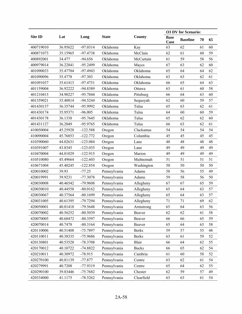
2A-58
Site ID Lat Long State County O3 DV for Scenario: Base Case
Baseline 70 65
400719010 36.95622 -97.0314 Oklahoma Kay 63 62 61 60
400871073 35.15965 -97.4738 Oklahoma McClain 62 61 60 59
400892001 34.477 -94.656 Oklahoma McCurtain 61 59 58 56
400979014 36.22841 -95.2499 Oklahoma Mayes 67 63 62 60
401090033 35.47704 -97.4943 Oklahoma Oklahoma 65 64 64 62
401090096 35.4778 -97.303 Oklahoma Oklahoma 63 63 62 61
401091037 35.61413 -97.4751 Oklahoma Oklahoma 66 65 64 63
401159004 36.92222 -94.8389 Oklahoma Ottawa 63 61 60 58
401210415 34.90227 -95.7844 Oklahoma Pittsburg 66 64 63 60
401359021 35.40814 -94.5244 Oklahoma Sequoyah 62 60 59 57
401430137 36.35744 -95.9992 Oklahoma Tulsa 65 63 62 61
401430174 35.95371 -96.005 Oklahoma Tulsa 64 60 60 59
401430178 36.1338 -95.7645 Oklahoma Tulsa 65 62 62 60
401431127 36.2049 -95.9765 Oklahoma Tulsa 66 63 62 61
410050004 45.25928 -122.588 Oregon Clackamas 54 54 54 54
410090004 45.76853 -122.772 Oregon Columbia 45 45 45 45
410390060 44.02631 -123.084 Oregon Lane 48 48 48 48
410391007 43.8345 -123.035 Oregon Lane 49 49 49 49
410470004 44.81029 -122.915 Oregon Marion 49 49 49 49
410510080 45.49664 -122.603 Oregon Multnomah 51 51 51 51
410671004 45.40245 -122.854 Oregon Washington 50 50 50 50
420010002 39.93 -77.25 Pennsylvania Adams 58 56 55 49
420019991 39.9231 -77.3078 Pennsylvania Adams 59 58 56 50
420030008 40.46542 -79.9608 Pennsylvania Allegheny 67 67 65 59
420030010 40.44558 -80.0162 Pennsylvania Allegheny 65 64 63 57
420030067 40.37564 -80.1699 Pennsylvania Allegheny 65 64 63 57
420031005 40.61395 -79.7294 Pennsylvania Allegheny 71 71 69 62
420050001 40.81418 -79.5648 Pennsylvania Armstrong 65 64 63 56
420070002 40.56252 -80.5039 Pennsylvania Beaver 62 62 61 58
420070005 40.68472 -80.3597 Pennsylvania Beaver 66 66 65 59
420070014 40.7478 -80.3164 Pennsylvania Beaver 65 64 63 58
420110006 40.51408 -75.7897 Pennsylvania Berks 59 57 55 48
420110011 40.38335 -75.9686 Pennsylvania Berks 63 61 59 52
420130801 40.53528 -78.3708 Pennsylvania Blair 66 64 62 55
420170012 40.10722 -74.8822 Pennsylvania Bucks 66 65 62 54
420210011 40.30972 -78.915 Pennsylvania Cambria 61 60 58 52
420270100 40.81139 -77.877 Pennsylvania Centre 63 62 61 54
420279991 40.7208 -77.9319 Pennsylvania Centre 65 64 62 55
420290100 39.83446 -75.7682 Pennsylvania Chester 62 59 57 49
420334000 41.1175 -78.5262 Pennsylvania Clearfield 63 63 61 54
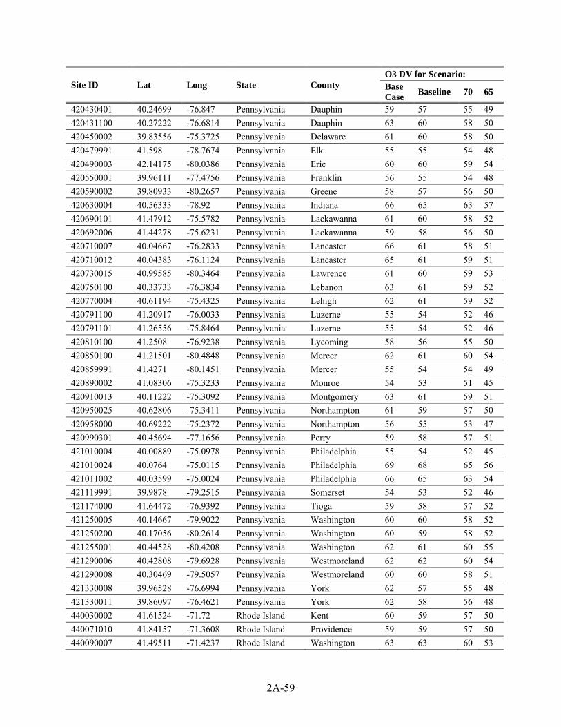
2A-59
Site ID Lat Long State County O3 DV for Scenario: Base Case
Baseline 70 65
420430401 40.24699 -76.847 Pennsylvania Dauphin 59 57 55 49
420431100 40.27222 -76.6814 Pennsylvania Dauphin 63 60 58 50
420450002 39.83556 -75.3725 Pennsylvania Delaware 61 60 58 50
420479991 41.598 -78.7674 Pennsylvania Elk 55 55 54 48
420490003 42.14175 -80.0386 Pennsylvania Erie 60 60 59 54
420550001 39.96111 -77.4756 Pennsylvania Franklin 56 55 54 48
420590002 39.80933 -80.2657 Pennsylvania Greene 58 57 56 50
420630004 40.56333 -78.92 Pennsylvania Indiana 66 65 63 57
420690101 41.47912 -75.5782 Pennsylvania Lackawanna 61 60 58 52
420692006 41.44278 -75.6231 Pennsylvania Lackawanna 59 58 56 50
420710007 40.04667 -76.2833 Pennsylvania Lancaster 66 61 58 51
420710012 40.04383 -76.1124 Pennsylvania Lancaster 65 61 59 51
420730015 40.99585 -80.3464 Pennsylvania Lawrence 61 60 59 53
420750100 40.33733 -76.3834 Pennsylvania Lebanon 63 61 59 52
420770004 40.61194 -75.4325 Pennsylvania Lehigh 62 61 59 52
420791100 41.20917 -76.0033 Pennsylvania Luzerne 55 54 52 46
420791101 41.26556 -75.8464 Pennsylvania Luzerne 55 54 52 46
420810100 41.2508 -76.9238 Pennsylvania Lycoming 58 56 55 50
420850100 41.21501 -80.4848 Pennsylvania Mercer 62 61 60 54
420859991 41.4271 -80.1451 Pennsylvania Mercer 55 54 54 49
420890002 41.08306 -75.3233 Pennsylvania Monroe 54 53 51 45
420910013 40.11222 -75.3092 Pennsylvania Montgomery 63 61 59 51
420950025 40.62806 -75.3411 Pennsylvania Northampton 61 59 57 50
420958000 40.69222 -75.2372 Pennsylvania Northampton 56 55 53 47
420990301 40.45694 -77.1656 Pennsylvania Perry 59 58 57 51
421010004 40.00889 -75.0978 Pennsylvania Philadelphia 55 54 52 45
421010024 40.0764 -75.0115 Pennsylvania Philadelphia 69 68 65 56
421011002 40.03599 -75.0024 Pennsylvania Philadelphia 66 65 63 54
421119991 39.9878 -79.2515 Pennsylvania Somerset 54 53 52 46
421174000 41.64472 -76.9392 Pennsylvania Tioga 59 58 57 52
421250005 40.14667 -79.9022 Pennsylvania Washington 60 60 58 52
421250200 40.17056 -80.2614 Pennsylvania Washington 60 59 58 52
421255001 40.44528 -80.4208 Pennsylvania Washington 62 61 60 55
421290006 40.42808 -79.6928 Pennsylvania Westmoreland 62 62 60 54
421290008 40.30469 -79.5057 Pennsylvania Westmoreland 60 60 58 51
421330008 39.96528 -76.6994 Pennsylvania York 62 57 55 48
421330011 39.86097 -76.4621 Pennsylvania York 62 58 56 48
440030002 41.61524 -71.72 Rhode Island Kent 60 59 57 50
440071010 41.84157 -71.3608 Rhode Island Providence 59 59 57 50
440090007 41.49511 -71.4237 Rhode Island Washington 63 63 60 53

2A-60
Site ID Lat Long State County O3 DV for Scenario: Base Case
Baseline 70 65
450010001 34.32532 -82.3864 South Carolina Abbeville 47 46 46 44
450030003 33.34223 -81.7887 South Carolina Aiken 49 48 48 47
450070005 34.62324 -82.5321 South Carolina Anderson 53 52 52 51
450150002 32.98725 -79.9367 South Carolina Berkeley 49 49 49 48
450190046 32.94102 -79.6572 South Carolina Charleston 51 50 50 49
450250001 34.61537 -80.1988 South Carolina Chesterfield 50 50 49 48
450290002 33.00787 -80.965 South Carolina Colleton 48 47 47 45
450310003 34.2857 -79.7449 South Carolina Darlington 53 52 52 50
450370001 33.73996 -81.8536 South Carolina Edgefield 46 45 45 44
450450016 34.75185 -82.2567 South Carolina Greenville 52 51 51 50
450451003 35.0574 -82.3729 South Carolina Greenville 50 49 49 48
450770002 34.65361 -82.8387 South Carolina Pickens 54 53 53 51
450770003 34.85154 -82.7446 South Carolina Pickens 50 50 49 48
450790007 34.09396 -80.9623 South Carolina Richland 51 50 50 49
450790021 33.81468 -80.7811 South Carolina Richland 46 45 44 43
450791001 34.13126 -80.8683 South Carolina Richland 54 53 53 52
450830009 34.98871 -82.0758 South Carolina Spartanburg 56 55 55 54
450910006 34.93582 -81.2284 South Carolina York 50 49 49 48
460330132 43.5578 -103.484 South Dakota Custer 58 58 57 57
460710001 43.74561 -101.941 South Dakota Jackson 52 52 52 51
460930001 44.15564 -103.316 South Dakota Meade 53 53 52 52
460990008 43.54792 -96.7008 South Dakota Minnehaha 56 56 55 55
461270003 42.88021 -96.7853 South Dakota Union 54 53 53 52
470010101 35.96522 -84.2232 Tennessee Anderson 55 55 54 48
470090101 35.63149 -83.9435 Tennessee Blount 59 59 58 52
470090102 35.60306 -83.7836 Tennessee Blount 51 50 50 45
470259991 36.47 -83.8268 Tennessee Claiborne 48 47 47 43
470370011 36.205 -86.7447 Tennessee Davidson 52 52 51 46
470370026 36.15074 -86.6233 Tennessee Davidson 56 55 55 49
470419991 36.0388 -85.7331 Tennessee DeKalb 54 54 53 49
470651011 35.23348 -85.1816 Tennessee Hamilton 55 55 54 50
470654003 35.10264 -85.1622 Tennessee Hamilton 56 55 54 50
470890002 36.10563 -83.6021 Tennessee Jefferson 58 57 56 51
470930021 36.08551 -83.7648 Tennessee Knox 53 53 52 47
470931020 36.01919 -83.8738 Tennessee Knox 55 54 54 48
471050109 35.72089 -84.3422 Tennessee Loudon 57 56 55 49
471210104 35.28938 -84.9461 Tennessee Meigs 55 54 54 50
471490101 35.73288 -86.5989 Tennessee Rutherford 53 53 52 47
471550101 35.69667 -83.6097 Tennessee Sevier 57 57 56 52
471550102 35.56278 -83.4981 Tennessee Sevier 57 56 56 52

2A-61
Site ID Lat Long State County O3 DV for Scenario: Base Case
Baseline 70 65
471570021 35.2175 -90.0197 Tennessee Shelby 60 59 58 52
471570075 35.1517 -89.8502 Tennessee Shelby 61 60 59 53
471571004 35.37815 -89.8345 Tennessee Shelby 58 57 56 51
471632002 36.54144 -82.4248 Tennessee Sullivan 60 60 59 53
471632003 36.58211 -82.4857 Tennessee Sullivan 59 59 59 53
471650007 36.29756 -86.6531 Tennessee Sumner 60 60 59 54
471650101 36.45398 -86.5641 Tennessee Sumner 57 56 56 51
471870106 35.95153 -87.137 Tennessee Williamson 55 55 54 48
471890103 36.06083 -86.2863 Tennessee Wilson 57 57 56 52
480271047 31.088 -97.6797 Texas Bell 63 62 60 56
480290032 29.51509 -98.6202 Texas Bexar 67 66 63 59
480290052 29.63206 -98.5649 Texas Bexar 68 67 64 60
480290059 29.27538 -98.3117 Texas Bexar 60 59 57 53
480391004 29.52044 -95.3925 Texas Brazoria 76 75 70 64
480391016 29.04376 -95.4729 Texas Brazoria 64 63 61 57
480610006 25.8925 -97.4938 Texas Cameron 57 57 56 54
480850005 33.13242 -96.7864 Texas Collin 69 68 64 58
481130069 32.81995 -96.8601 Texas Dallas 69 68 64 58
481130075 32.91921 -96.8085 Texas Dallas 70 69 65 59
481130087 32.67645 -96.8721 Texas Dallas 69 68 64 58
481210034 33.21906 -97.1963 Texas Denton 71 70 66 60
481211032 33.41064 -96.9446 Texas Denton 70 69 65 59
481390016 32.48208 -97.0269 Texas Ellis 66 65 62 57
481391044 32.17543 -96.8702 Texas Ellis 61 60 57 53
481410029 31.78577 -106.324 Texas El Paso 54 54 54 54
481410037 31.76829 -106.501 Texas El Paso 62 62 62 61
481410044 31.7657 -106.455 Texas El Paso 60 60 60 60
481410055 31.74674 -106.403 Texas El Paso 58 58 58 58
481410057 31.6675 -106.288 Texas El Paso 57 57 57 57
481410058 31.89391 -106.426 Texas El Paso 61 60 60 60
481671034 29.25447 -94.8613 Texas Galveston 70 69 67 64
481830001 32.37868 -94.7118 Texas Gregg 70 66 62 55
482010024 29.90104 -95.3261 Texas Harris 71 70 66 60
482010026 29.80271 -95.1255 Texas Harris 70 69 66 61
482010029 30.03953 -95.6739 Texas Harris 69 68 64 59
482010046 29.82809 -95.2841 Texas Harris 67 66 62 57
482010047 29.83472 -95.4892 Texas Harris 67 66 62 55
482010051 29.62361 -95.4736 Texas Harris 69 68 64 58
482010055 29.69574 -95.4993 Texas Harris 70 69 65 58
482010062 29.62583 -95.2675 Texas Harris 68 67 63 57
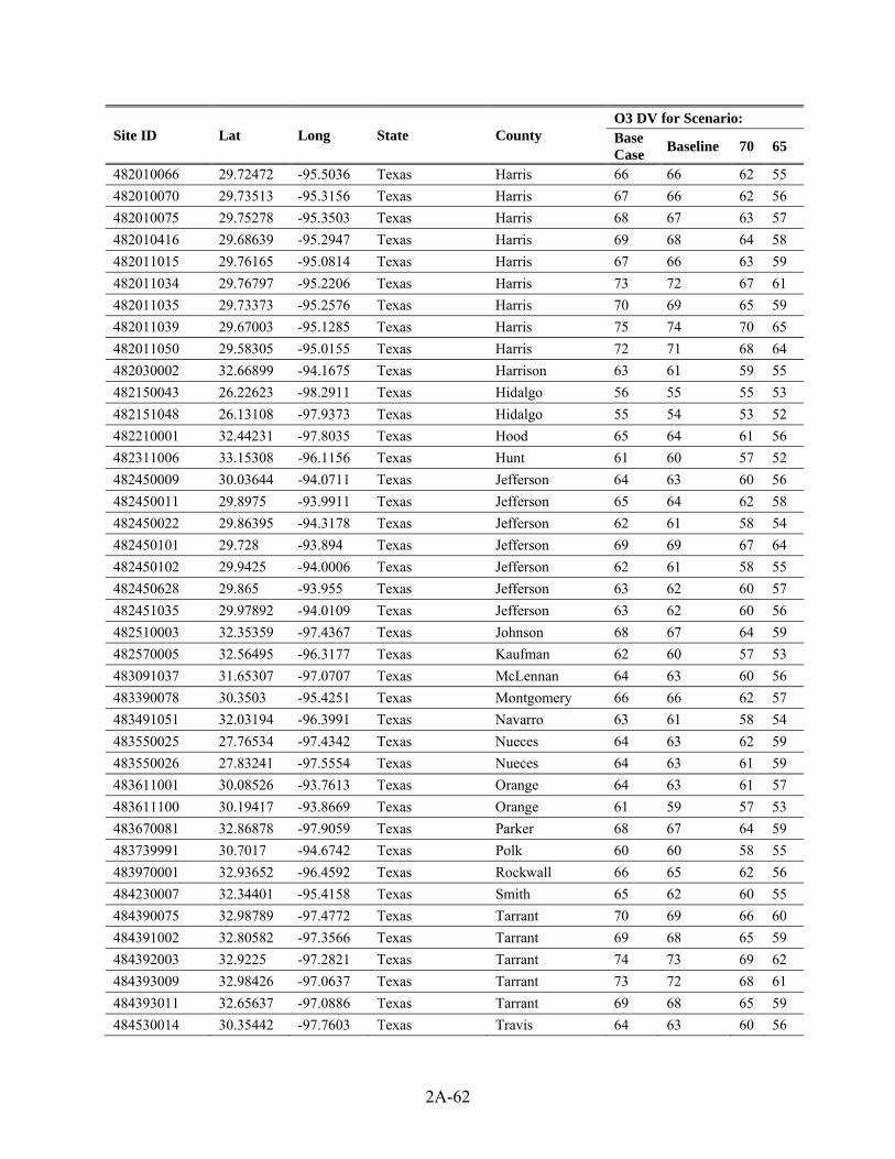
2A-62
Site ID Lat Long State County O3 DV for Scenario: Base Case
Baseline 70 65
482010066 29.72472 -95.5036 Texas Harris 66 66 62 55
482010070 29.73513 -95.3156 Texas Harris 67 66 62 56
482010075 29.75278 -95.3503 Texas Harris 68 67 63 57
482010416 29.68639 -95.2947 Texas Harris 69 68 64 58
482011015 29.76165 -95.0814 Texas Harris 67 66 63 59
482011034 29.76797 -95.2206 Texas Harris 73 72 67 61
482011035 29.73373 -95.2576 Texas Harris 70 69 65 59
482011039 29.67003 -95.1285 Texas Harris 75 74 70 65
482011050 29.58305 -95.0155 Texas Harris 72 71 68 64
482030002 32.66899 -94.1675 Texas Harrison 63 61 59 55
482150043 26.22623 -98.2911 Texas Hidalgo 56 55 55 53
482151048 26.13108 -97.9373 Texas Hidalgo 55 54 53 52
482210001 32.44231 -97.8035 Texas Hood 65 64 61 56
482311006 33.15308 -96.1156 Texas Hunt 61 60 57 52
482450009 30.03644 -94.0711 Texas Jefferson 64 63 60 56
482450011 29.8975 -93.9911 Texas Jefferson 65 64 62 58
482450022 29.86395 -94.3178 Texas Jefferson 62 61 58 54
482450101 29.728 -93.894 Texas Jefferson 69 69 67 64
482450102 29.9425 -94.0006 Texas Jefferson 62 61 58 55
482450628 29.865 -93.955 Texas Jefferson 63 62 60 57
482451035 29.97892 -94.0109 Texas Jefferson 63 62 60 56
482510003 32.35359 -97.4367 Texas Johnson 68 67 64 59
482570005 32.56495 -96.3177 Texas Kaufman 62 60 57 53
483091037 31.65307 -97.0707 Texas McLennan 64 63 60 56
483390078 30.3503 -95.4251 Texas Montgomery 66 66 62 57
483491051 32.03194 -96.3991 Texas Navarro 63 61 58 54
483550025 27.76534 -97.4342 Texas Nueces 64 63 62 59
483550026 27.83241 -97.5554 Texas Nueces 64 63 61 59
483611001 30.08526 -93.7613 Texas Orange 64 63 61 57
483611100 30.19417 -93.8669 Texas Orange 61 59 57 53
483670081 32.86878 -97.9059 Texas Parker 68 67 64 59
483739991 30.7017 -94.6742 Texas Polk 60 60 58 55
483970001 32.93652 -96.4592 Texas Rockwall 66 65 62 56
484230007 32.34401 -95.4158 Texas Smith 65 62 60 55
484390075 32.98789 -97.4772 Texas Tarrant 70 69 66 60
484391002 32.80582 -97.3566 Texas Tarrant 69 68 65 59
484392003 32.9225 -97.2821 Texas Tarrant 74 73 69 62
484393009 32.98426 -97.0637 Texas Tarrant 73 72 68 61
484393011 32.65637 -97.0886 Texas Tarrant 69 68 65 59
484530014 30.35442 -97.7603 Texas Travis 64 63 60 56
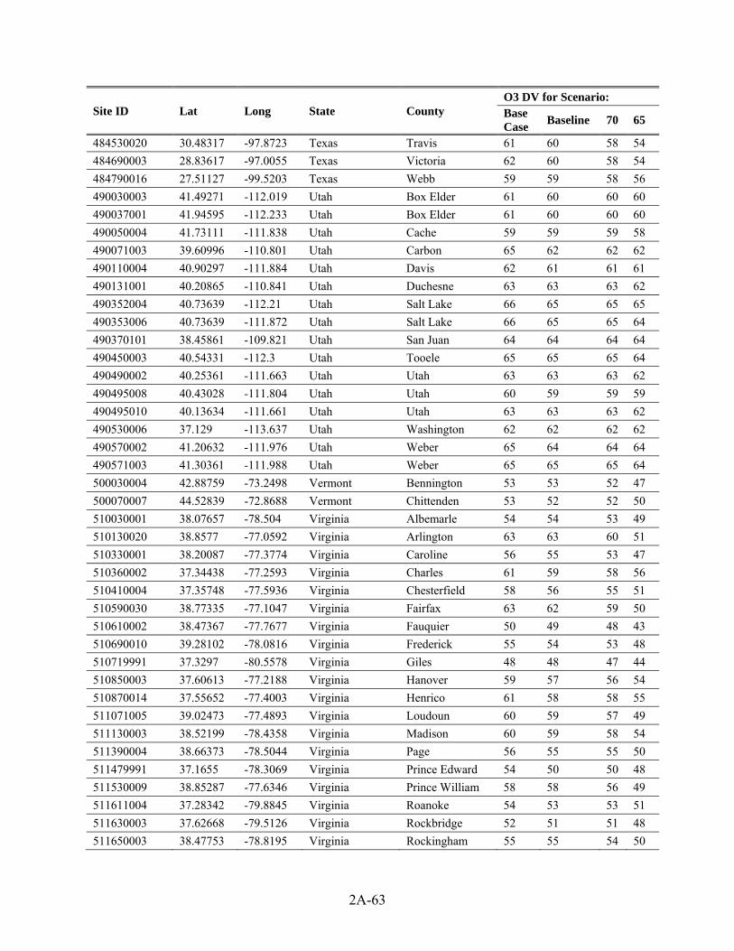
2A-63
Site ID Lat Long State County O3 DV for Scenario: Base Case
Baseline 70 65
484530020 30.48317 -97.8723 Texas Travis 61 60 58 54
484690003 28.83617 -97.0055 Texas Victoria 62 60 58 54
484790016 27.51127 -99.5203 Texas Webb 59 59 58 56
490030003 41.49271 -112.019 Utah Box Elder 61 60 60 60
490037001 41.94595 -112.233 Utah Box Elder 61 60 60 60
490050004 41.73111 -111.838 Utah Cache 59 59 59 58
490071003 39.60996 -110.801 Utah Carbon 65 62 62 62
490110004 40.90297 -111.884 Utah Davis 62 61 61 61
490131001 40.20865 -110.841 Utah Duchesne 63 63 63 62
490352004 40.73639 -112.21 Utah Salt Lake 66 65 65 65
490353006 40.73639 -111.872 Utah Salt Lake 66 65 65 64
490370101 38.45861 -109.821 Utah San Juan 64 64 64 64
490450003 40.54331 -112.3 Utah Tooele 65 65 65 64
490490002 40.25361 -111.663 Utah Utah 63 63 63 62
490495008 40.43028 -111.804 Utah Utah 60 59 59 59
490495010 40.13634 -111.661 Utah Utah 63 63 63 62
490530006 37.129 -113.637 Utah Washington 62 62 62 62
490570002 41.20632 -111.976 Utah Weber 65 64 64 64
490571003 41.30361 -111.988 Utah Weber 65 65 65 64
500030004 42.88759 -73.2498 Vermont Bennington 53 53 52 47
500070007 44.52839 -72.8688 Vermont Chittenden 53 52 52 50
510030001 38.07657 -78.504 Virginia Albemarle 54 54 53 49
510130020 38.8577 -77.0592 Virginia Arlington 63 63 60 51
510330001 38.20087 -77.3774 Virginia Caroline 56 55 53 47
510360002 37.34438 -77.2593 Virginia Charles 61 59 58 56
510410004 37.35748 -77.5936 Virginia Chesterfield 58 56 55 51
510590030 38.77335 -77.1047 Virginia Fairfax 63 62 59 50
510610002 38.47367 -77.7677 Virginia Fauquier 50 49 48 43
510690010 39.28102 -78.0816 Virginia Frederick 55 54 53 48
510719991 37.3297 -80.5578 Virginia Giles 48 48 47 44
510850003 37.60613 -77.2188 Virginia Hanover 59 57 56 54
510870014 37.55652 -77.4003 Virginia Henrico 61 58 58 55
511071005 39.02473 -77.4893 Virginia Loudoun 60 59 57 49
511130003 38.52199 -78.4358 Virginia Madison 60 59 58 54
511390004 38.66373 -78.5044 Virginia Page 56 55 55 50
511479991 37.1655 -78.3069 Virginia Prince Edward 54 50 50 48
511530009 38.85287 -77.6346 Virginia Prince William 58 58 56 49
511611004 37.28342 -79.8845 Virginia Roanoke 54 53 53 51
511630003 37.62668 -79.5126 Virginia Rockbridge 52 51 51 48
511650003 38.47753 -78.8195 Virginia Rockingham 55 55 54 50
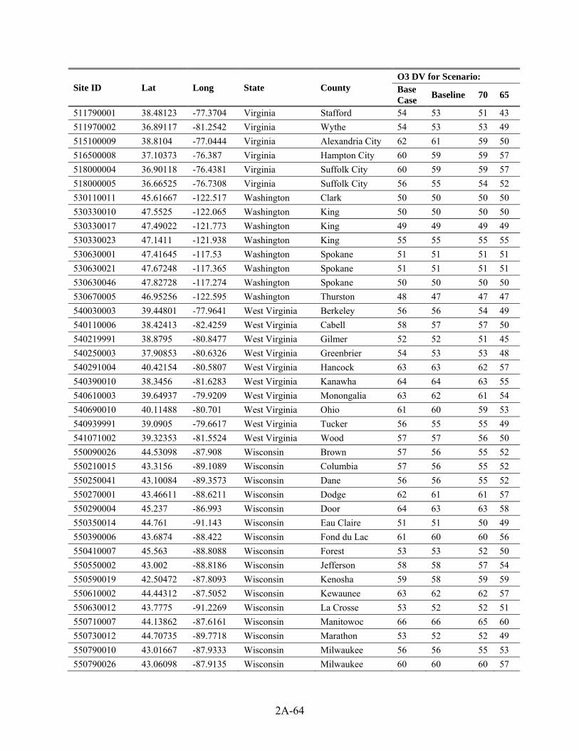
2A-64
Site ID Lat Long State County O3 DV for Scenario: Base Case
Baseline 70 65
511790001 38.48123 -77.3704 Virginia Stafford 54 53 51 43
511970002 36.89117 -81.2542 Virginia Wythe 54 53 53 49
515100009 38.8104 -77.0444 Virginia Alexandria City 62 61 59 50
516500008 37.10373 -76.387 Virginia Hampton City 60 59 59 57
518000004 36.90118 -76.4381 Virginia Suffolk City 60 59 59 57
518000005 36.66525 -76.7308 Virginia Suffolk City 56 55 54 52
530110011 45.61667 -122.517 Washington Clark 50 50 50 50
530330010 47.5525 -122.065 Washington King 50 50 50 50
530330017 47.49022 -121.773 Washington King 49 49 49 49
530330023 47.1411 -121.938 Washington King 55 55 55 55
530630001 47.41645 -117.53 Washington Spokane 51 51 51 51
530630021 47.67248 -117.365 Washington Spokane 51 51 51 51
530630046 47.82728 -117.274 Washington Spokane 50 50 50 50
530670005 46.95256 -122.595 Washington Thurston 48 47 47 47
540030003 39.44801 -77.9641 West Virginia Berkeley 56 56 54 49
540110006 38.42413 -82.4259 West Virginia Cabell 58 57 57 50
540219991 38.8795 -80.8477 West Virginia Gilmer 52 52 51 45
540250003 37.90853 -80.6326 West Virginia Greenbrier 54 53 53 48
540291004 40.42154 -80.5807 West Virginia Hancock 63 63 62 57
540390010 38.3456 -81.6283 West Virginia Kanawha 64 64 63 55
540610003 39.64937 -79.9209 West Virginia Monongalia 63 62 61 54
540690010 40.11488 -80.701 West Virginia Ohio 61 60 59 53
540939991 39.0905 -79.6617 West Virginia Tucker 56 55 55 49
541071002 39.32353 -81.5524 West Virginia Wood 57 57 56 50
550090026 44.53098 -87.908 Wisconsin Brown 57 56 55 52
550210015 43.3156 -89.1089 Wisconsin Columbia 57 56 55 52
550250041 43.10084 -89.3573 Wisconsin Dane 56 56 55 52
550270001 43.46611 -88.6211 Wisconsin Dodge 62 61 61 57
550290004 45.237 -86.993 Wisconsin Door 64 63 63 58
550350014 44.761 -91.143 Wisconsin Eau Claire 51 51 50 49
550390006 43.6874 -88.422 Wisconsin Fond du Lac 61 60 60 56
550410007 45.563 -88.8088 Wisconsin Forest 53 53 52 50
550550002 43.002 -88.8186 Wisconsin Jefferson 58 58 57 54
550590019 42.50472 -87.8093 Wisconsin Kenosha 59 58 59 59
550610002 44.44312 -87.5052 Wisconsin Kewaunee 63 62 62 57
550630012 43.7775 -91.2269 Wisconsin La Crosse 53 52 52 51
550710007 44.13862 -87.6161 Wisconsin Manitowoc 66 66 65 60
550730012 44.70735 -89.7718 Wisconsin Marathon 53 52 52 49
550790010 43.01667 -87.9333 Wisconsin Milwaukee 56 56 55 53
550790026 43.06098 -87.9135 Wisconsin Milwaukee 60 60 60 57
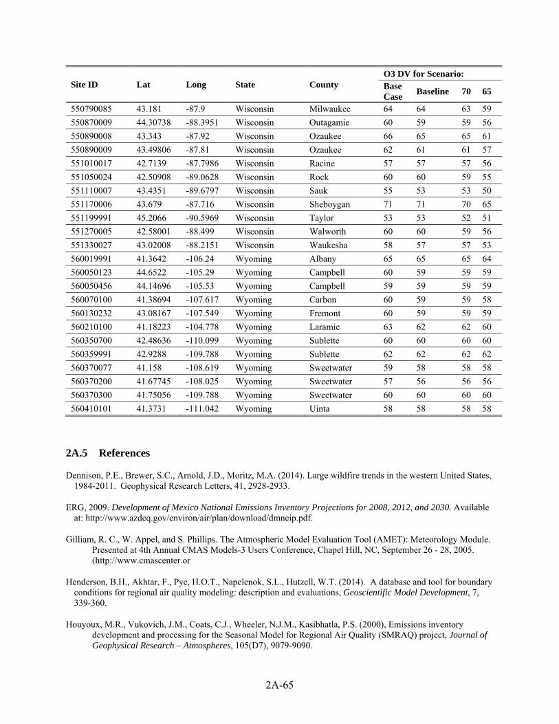
2A-65
Site ID Lat Long State County O3 DV for Scenario: Base Case
Baseline 70 65
550790085 43.181 -87.9 Wisconsin Milwaukee 64 64 63 59
550870009 44.30738 -88.3951 Wisconsin Outagamie 60 59 59 56
550890008 43.343 -87.92 Wisconsin Ozaukee 66 65 65 61
550890009 43.49806 -87.81 Wisconsin Ozaukee 62 61 61 57
551010017 42.7139 -87.7986 Wisconsin Racine 57 57 57 56
551050024 42.50908 -89.0628 Wisconsin Rock 60 60 59 55
551110007 43.4351 -89.6797 Wisconsin Sauk 55 53 53 50
551170006 43.679 -87.716 Wisconsin Sheboygan 71 71 70 65
551199991 45.2066 -90.5969 Wisconsin Taylor 53 53 52 51
551270005 42.58001 -88.499 Wisconsin Walworth 60 60 59 56
551330027 43.02008 -88.2151 Wisconsin Waukesha 58 57 57 53
560019991 41.3642 -106.24 Wyoming Albany 65 65 65 64
560050123 44.6522 -105.29 Wyoming Campbell 60 59 59 59
560050456 44.14696 -105.53 Wyoming Campbell 59 59 59 59
560070100 41.38694 -107.617 Wyoming Carbon 60 59 59 58
560130232 43.08167 -107.549 Wyoming Fremont 60 59 59 59
560210100 41.18223 -104.778 Wyoming Laramie 63 62 62 60
560350700 42.48636 -110.099 Wyoming Sublette 60 60 60 60
560359991 42.9288 -109.788 Wyoming Sublette 62 62 62 62
560370077 41.158 -108.619 Wyoming Sweetwater 59 58 58 58
560370200 41.67745 -108.025 Wyoming Sweetwater 57 56 56 56
560370300 41.75056 -109.788 Wyoming Sweetwater 60 60 60 60
560410101 41.3731 -111.042 Wyoming Uinta 58 58 58 58
2A.5 References
Dennison, P.E., Brewer, S.C., Arnold, J.D., Moritz, M.A. (2014). Large wildfire trends in the western United States, 1984-2011. Geophysical Research Letters, 41, 2928-2933.
ERG, 2009. Development of Mexico National Emissions Inventory Projections for 2008, 2012, and 2030. Available at: http://www.azdeq.gov/environ/air/plan/download/dmneip.pdf.
Gilliam, R. C., W. Appel, and S. Phillips. The Atmospheric Model Evaluation Tool (AMET): Meteorology Module. Presented at 4th Annual CMAS Models-3 Users Conference, Chapel Hill, NC, September 26 - 28, 2005. (http://www.cmascenter.or
Henderson, B.H., Akhtar, F., Pye, H.O.T., Napelenok, S.L., Hutzell, W.T. (2014). A database and tool for boundary conditions for regional air quality modeling: description and evaluations, Geoscientific Model Development, 7, 339-360.
Houyoux, M.R., Vukovich, J.M., Coats, C.J., Wheeler, N.J.M., Kasibhatla, P.S. (2000), Emissions inventory development and processing for the Seasonal Model for Regional Air Quality (SMRAQ) project, Journal of Geophysical Research – Atmospheres, 105(D7), 9079-9090.

2A-66
Karl, T. R. and Koss, W. J., 1984: "Regional and National Monthly, Seasonal, and Annual Temperature Weighted by Area, 1895-1983." Historical Climatology Series 4-3, National Climatic Data Center, Asheville, NC, 38 pp.
National Research Council (NRC), 2002. Estimating the Public Health Benefits of Proposed Air Pollution Regulations, Washington, DC: National Academies Press.
Phillips, S., K. Wang, C. Jang, N. Possiel, M. Strum, T. Fox, 2007: Evaluation of 2002 Multi-pollutant Platform: Air Toxics, Ozone, and Particulate Matter, 7th Annual CMAS Conference, Chapel Hill, NC, October 6-8, 2008.
Ruiz, L.H., Yarwood, G., 2013. Interactions between Organic Aerosol and NOy: Influence on Oxidant Production. http://aqrp.ceer.utexas.edu/projectinfoFY12_13/12-012/12-012%20Final%20Report.pdf.
Skamarock, W.C., Klemp, J.B., Dudhia, J., Gill, D.O., Barker, D.M., Duda, M.G., Huang, X., Wang, W., Powers, J.G., 2008, A description of the advanced research WRF version 3, National Center for Atmospheric Research, Boulder, CO, USA, NCAR/TN-475+STR
Simon, H., Baker, K., Phillips, S., 2012: Compilation and interpretation of photochemical model performance statistics published between 2006 and 2012. Atmospheric Environment 61, 124-139.
U.S. Environmental Protection Agency (US EPA), 2005; Technical Support Document for the Final Clean Air Interstate Rule: Air Quality Modeling; Office of Air Quality Planning and Standards; RTP, NC; (CAIR Docket OAR-2005-0053-2149).
U.S. Environmental Protection Agency (US EPA) 2009; Technical Support Document for the Proposal to Designate an Emissions Control Area for Nitrogen Oxides, Sulfur Oxides, and Particulate Matter: EPA-420-R-007, 329pp. (http://www.epa.gov/otaq/regs/nonroad/marine/ci/420r09007.pdf)
U.S. Environmental Protection Agency (2014a) Meteorological Model Performance for Annual 2011 Simulation WRF v3.4, US EPA, OAQPS, 2014, RTP, NC http://www.epa.gov/scram001/
U.S. Environmental Protection Agency (2014b) Preparation of Emissions Inventories for the Version 6.1, 2011 Emissions Modeling Platform (http://www.epa.gov/ttn/chief/emch)
U.S. Environmental Protection Agency (US EPA) 2014c; Draft Modeling Guidance for demonstrating attainment of air quality goals for ozone, PM2.5, and regional haze. September 2014, U.S. Environmental Protection Agency, Research Triangle Park, NC, 27711.
U.S. Environmental Protection Agency (US EPA), 2014d; Regulatory Impact Analysis of the Proposed Revisions to the National Ambient Air Quality Standards for Ground-Level Ozone, Office of Air Quality Planning and Standards; RTP, NC, EPA-452/P-14-006
Yantosca, B. and Carouge, C., 2010, GEOS-Chem v8-03-01 User’s Guide, Atmospheric Chemistry Modeling Group, Harvard University, Cambridge, MA, http://acmg.seas.harvard.edu/geos/doc/archive/man.v8-03-02/index.html

3-1
CHAPTER 3 : CONTROL STRATEGIES AND EMISSIONS REDUCTIONS
Overview
To estimate the costs and benefits of alternative ozone standard levels, the EPA has
analyzed hypothetical control strategies that areas across the country might employ to attain the
revised ozone standard level of 70 ppb and a more stringent alternative standard of 65 ppb. The
future year for analyzing the incremental costs and benefits of meeting a revised ozone standard
is 2025.44 This analysis year was chosen because most areas of the U.S. will be required to meet
a revised ozone standard by 2025. California was analyzed independently from the rest of the
U.S. because of the potential for longer compliance timelines in many areas. Consequently, we
created two baseline scenarios, a 2025 baseline for all areas outside of California and a post-2025
baseline for California.
This chapter documents the (i) emissions control measures EPA applied to illustrate
attainment with the revised ozone standard of 70 ppb and the alternative standard of 65 ppb and
(ii) projected emissions reductions associated with the measures. The chapter is organized into
five sections. Section 3.1 provides a summary of the steps that we took to determine necessary
emissions reductions to create the 2025 baseline and the control strategies to reach the revised
standard level of 70 ppb and an alternative standard of 65 ppb in the continental U.S. outside of
California. Section 3.2 describes the steps we took to determine necessary emissions reductions
to create the post 2025-baseline and the control strategy to reach 70 ppb and 65 ppb for
California. In Section 3.3 we discuss key differences between the results from the analysis
conducted for the proposal RIA and this analysis. In Section 3.4 we list the key limitations and
uncertainties associated with the control strategy analysis. And finally, Section 3.5 includes the
references for the chapter.
To conduct the control strategy analyses, we first require information on total emissions
reductions needed to simulate attainment. For that purpose we need (i) projected future design
value and design value (DV) targets for each area, (ii) the sensitivity of ozone DVs to the NOx
44 Please see Chapter 1, Section 1.3.2 for a detailed discussion of the potential nonattainment designations and their timing.

3-2
and VOC emissions reductions, and (iii) available NOx and VOC reductions from identified
controls (as will be described in section 3.1.1). Second, to find an illustrative control strategy to
achieve the emissions reductions needed, we need information about available identified
controls45 for specific sources and associated emissions reductions. More details on air quality
modeling and information about projected future DVs, DV targets, and ppb/ton ozone response
factors are provided in Chapter 2. In this chapter we calculate the necessary emissions
reductions and describe the creation of hypothetical control strategies for the post-2025 baseline
and for the revised and alternative standard levels analyzed.
3.1 The 2025 Control Strategy Scenarios
To create the baseline, we projected 2025 ozone DVs for the base case scenario as
described in Section 2.2 of Chapter 2. We adjusted the 2025 base case for all areas of the U.S. to
account for emissions reductions from the Clean Power Plan in creating the 2025 baseline. In
addition, because in the final 2025 base case projections no monitors outside of California were
projected to violate the current standard of 75 ppb, no additional controls were applied to create
the 2025 baseline.
3.1.1 Approach for the Revised Standard of 70 ppb and Alternative Standard of 65 ppb
The control strategies applied to illustrate attainment of the revised and alternative
standards analyzed involved several steps. We applied regional and local ppb/ton ozone
response factors to estimate resulting ozone DVs at air quality monitor locations to find the
target emissions levels. Then we applied controls to reach those targets levels. These steps are
described in this section.
As described in Chapter 2, we performed a series of photochemical modeling simulations
to determine the response of ozone DVs at monitor locations to emissions reductions in specific
45 In the proposal RIA we discuss emissions reductions resulting from the application of known controls, as well as emissions reductions beyond known controls, using the terminology of “known controls” and “unknown controls.” In the final RIA, we have used slightly different terminology, consistent with past NAAQS RIAs. Here we refer to emissions reductions and controls as either “identified” controls or measures or “unidentified” controls or measures reflecting that unidentified controls or measures can include existing controls or measures for which the EPA does not have sufficient data to accurately estimate their costs.
3-3
regions (NOx emissions reductions) and urban areas (VOC emissions reductions). We estimated
the necessary emissions reductions sequentially, one region at a time. For each air quality
sensitivity region (see Chapter 2, Figure 2-2 for a map of the sensitivity regions), we determined
the amount of emissions reductions necessary for all monitors within the region to meet the
standard level analyzed.
To implement this approach, we ranked the monitors in descending order by baseline
DV, and the region that included the monitor with the highest projected baseline DV (East
Texas) was analyzed first. We estimated the emissions reductions to decrease ozone
concentrations to the level needed for that region. We then estimated the impact that those
emissions reductions would have on all other remaining regions. After emissions reductions
were estimated for each region, the remaining monitors were re-ordered based on the resulting
DVs and the next region with the highest baseline DV was targeted for emissions reductions, if
needed, and the impact of its reductions were estimated for the remaining regions. We repeated
this process until all regions had been analyzed. For each region analyzed, we determined (i) the
quantity of emissions reductions from available identified NOx & VOC controls, and (ii) the
impact of these controls on ozone concentrations. If additional decreases in ozone
concentrations were needed in the region being analyzed, additional emissions reductions would
have to come from unidentified controls. Figure 3-1 shows a summary of this process. A
numeric example of the calculation methodology is provided in Appendix 3A. In addition,
ozone DVs at all evaluated monitors are provided for each scenario in Appendix 2A, Section
2A.4.

3-4
Figure 3-1. Process to Find Needed Reductions to Reach the Revised and Alternative Standards
Because emissions reductions in NOx and VOC have different resulting air quality
impacts on ozone and because different combinations of reductions from these pollutants could
potentially render the same reduction in ozone, it is important to know for each region, a-priori,
the total potential available reductions of these two pollutants from identified controls. To find
these potentially available tons of NOx and VOC emissions reductions, we ran a maximum
emissions reductions run using CoST (Control Strategy Tool) (a description of CoST, its
algorithms, and the control strategy applied to obtain the necessary reductions follows in section
3.1.2), and applied the reductions from these controls as part of the process described above to
obtain the total needed emissions reductions. First, we estimated the available NOx and VOC
emissions reductions from identified controls to determine the reductions in ozone
concentrations. In this analysis, identified VOC controls are generally more expensive than
identified NOx controls and are only effective at reducing ozone in a limited number of
locations. For completeness, we applied the more expensive identified VOC controls in these
locations before applying any unidentified controls. Then we estimated any additional NOX
emissions reductions needed from unidentified controls to achieve the target reduction. We did
not apply any unidentified VOC controls.46 States will likely pursue the most effective controls
46 Past air quality modeling experience has indicated that in most areas NOx emissions reductions are more effective at reducing ozone concentrations at the monitor with the highest DV.
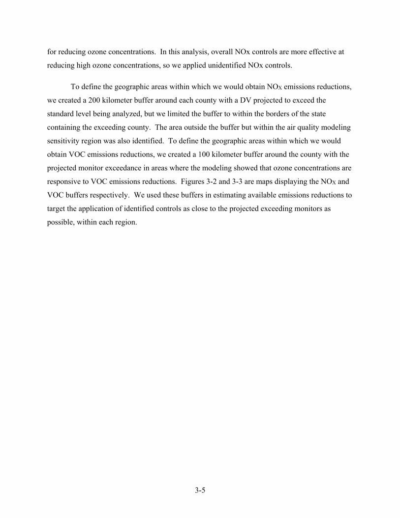
3-5
for reducing ozone concentrations. In this analysis, overall NOx controls are more effective at
reducing high ozone concentrations, so we applied unidentified NOx controls.
To define the geographic areas within which we would obtain NOX emissions reductions,
we created a 200 kilometer buffer around each county with a DV projected to exceed the
standard level being analyzed, but we limited the buffer to within the borders of the state
containing the exceeding county. The area outside the buffer but within the air quality modeling
sensitivity region was also identified. To define the geographic areas within which we would
obtain VOC emissions reductions, we created a 100 kilometer buffer around the county with the
projected monitor exceedance in areas where the modeling showed that ozone concentrations are
responsive to VOC emissions reductions. Figures 3-2 and 3-3 are maps displaying the NOX and
VOC buffers respectively. We used these buffers in estimating available emissions reductions to
target the application of identified controls as close to the projected exceeding monitors as
possible, within each region.

3-6
Figure 3-2. Buffers of 200 km for NOx Emissions Reductions around Projected Exceedance Areas
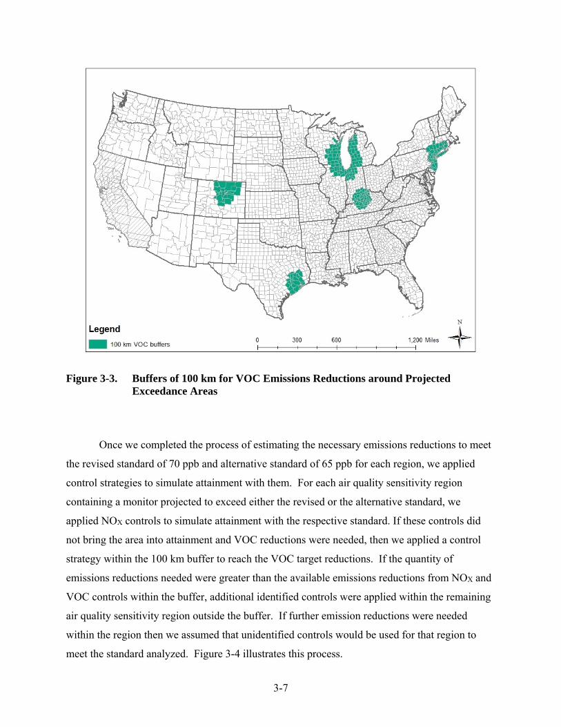
3-7
Figure 3-3. Buffers of 100 km for VOC Emissions Reductions around Projected Exceedance Areas
Once we completed the process of estimating the necessary emissions reductions to meet
the revised standard of 70 ppb and alternative standard of 65 ppb for each region, we applied
control strategies to simulate attainment with them. For each air quality sensitivity region
containing a monitor projected to exceed either the revised or the alternative standard, we
applied NOX controls to simulate attainment with the respective standard. If these controls did
not bring the area into attainment and VOC reductions were needed, then we applied a control
strategy within the 100 km buffer to reach the VOC target reductions. If the quantity of
emissions reductions needed were greater than the available emissions reductions from NOX and
VOC controls within the buffer, additional identified controls were applied within the remaining
air quality sensitivity region outside the buffer. If further emission reductions were needed
within the region then we assumed that unidentified controls would be used for that region to
meet the standard analyzed. Figure 3-4 illustrates this process.

3-8
Figure 3-4. Process to Estimate the Control Strategies for the Revised and Alternative Standards
3.1.2 Identified Control Measures
Control measures applied to meet the revised and alternative standards were identified for
four emissions sectors: Electric Generating Units (EGUs), Non-Electric Generating Unit Point
Sources (Non-EGUs), Nonpoint (Area) Sources, and Nonroad Mobile Sources. Onroad mobile
source controls were not applied because they are largely addressed in existing rules such as the
Tier 3 rule (U.S. EPA, 2014a). Controls applied for the revised and alternative standard analyses
are listed in Table 3-1.
The control measures we applied were identified using the EPA’s Control Strategy Tool
(CoST) (U.S. EPA, 2014b), the NONROAD Model (U.S. EPA, 2005) and the Integrated
Planning Model (IPM) (U.S. EPA, 2015).47 CoST models emissions reductions and engineering
costs associated with control strategies applied to non-EGUs, area, and mobile sources of air
pollutant emissions by matching control measures to emissions sources using algorithms such as
47 For the final RIA, an updated version of IPM was used. As a result of the updated version of IPM, after accounting for emissions reductions from the proposed Clean Power Plan we applied fewer controls to EGU sources than we applied in the proposal RIA.

3-9
"maximum emissions reduction", "least cost", and "apply measures in series". For this control
strategy analysis, we applied both the maximum emissions reduction (when all available
reductions were needed) and least cost algorithms48 (when not all available reductions were
needed). These controls are described further in Appendix 3A.
Nonpoint and nonroad mobile source emissions data are generated at the county level,
and therefore controls for these emissions sectors were applied at the county level. EGU and
non-EGU point source controls are applied to individual point sources. Control measures were
applied to non-EGU point and nonpoint sources of NOx, including: industrial boilers,
commercial and institutional boilers, reciprocating internal combustion engines in the oil and gas
industry and other industries, glass manufacturing furnaces, and cement kilns. The analysis for
nonroad mobile sources applied NOx controls to diesel engines. VOC controls applied included
surface coating, solvents, and fuel storage tanks.
To more accurately depict available controls, the EPA employed a decision rule in which
controls were not applied to any non-EGU point or nonpoint sources with less than 25 tons/year
of emissions per pollutant for NOX and 10 tons/year for VOC. This decision rule is more
inclusive of sources than the decision rule employed in the previous Ozone and PM2.5 NAAQS
RIAs where we applied a minimum of 50 tons/year for each pollutant. The reason for not
applying controls to sources below these levels is that many of these sources likely already have
controls in place that may not be reflected in the emissions inventory inputs, and we don’t
believe it is cost effective to apply an additional control device (see Chapter 4, Section 4.1.1 for a
brief discussion of the emissions inventory inputs). Furthermore, controls were not applied if
their cost per ton exceeded $19,000/ton for NOx or $33,000/ton for VOC (see Chapter 4, Section
4.1.1 for a discussion about these cutoff values). In addition, we only apply controls that replace
existing controls if replacement controls are at least 10% more effective than the existing control.
This is because we assume that replacement below that level would not be cost effective.
48 A maximum emissions reductions run in CoST will yield the same result as a least cost control strategy run with 100% control.
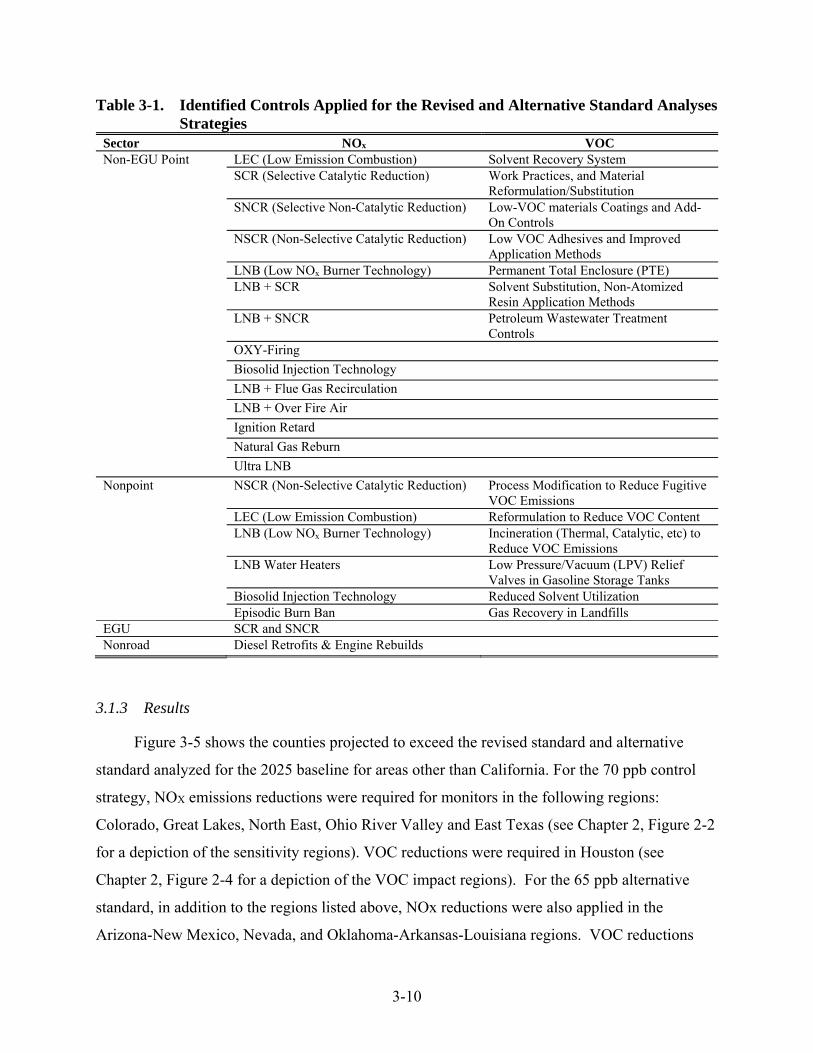
3-10
Table 3-1. Identified Controls Applied for the Revised and Alternative Standard Analyses Strategies
Sector NOx VOC Non-EGU Point LEC (Low Emission Combustion) Solvent Recovery System
SCR (Selective Catalytic Reduction) Work Practices, and Material Reformulation/Substitution
SNCR (Selective Non-Catalytic Reduction) Low-VOC materials Coatings and Add-On Controls
NSCR (Non-Selective Catalytic Reduction) Low VOC Adhesives and Improved Application Methods
LNB (Low NOx Burner Technology) Permanent Total Enclosure (PTE)LNB + SCR Solvent Substitution, Non-Atomized
Resin Application Methods LNB + SNCR Petroleum Wastewater Treatment
ControlsOXY-Firing Biosolid Injection Technology LNB + Flue Gas Recirculation LNB + Over Fire Air Ignition Retard Natural Gas Reburn Ultra LNB
Nonpoint NSCR (Non-Selective Catalytic Reduction) Process Modification to Reduce Fugitive VOC Emissions
LEC (Low Emission Combustion) Reformulation to Reduce VOC ContentLNB (Low NOx Burner Technology) Incineration (Thermal, Catalytic, etc) to
Reduce VOC Emissions LNB Water Heaters Low Pressure/Vacuum (LPV) Relief
Valves in Gasoline Storage TanksBiosolid Injection Technology Reduced Solvent Utilization Episodic Burn Ban Gas Recovery in Landfills
EGU SCR and SNCR Nonroad Diesel Retrofits & Engine Rebuilds
3.1.3 Results
Figure 3-5 shows the counties projected to exceed the revised standard and alternative
standard analyzed for the 2025 baseline for areas other than California. For the 70 ppb control
strategy, NOX emissions reductions were required for monitors in the following regions:
Colorado, Great Lakes, North East, Ohio River Valley and East Texas (see Chapter 2, Figure 2-2
for a depiction of the sensitivity regions). VOC reductions were required in Houston (see
Chapter 2, Figure 2-4 for a depiction of the VOC impact regions). For the 65 ppb alternative
standard, in addition to the regions listed above, NOx reductions were also applied in the
Arizona-New Mexico, Nevada, and Oklahoma-Arkansas-Louisiana regions. VOC reductions

3-11
were required in Denver, Houston, Louisville, Chicago and New York City.49 It is important to
note that for both the 70 ppb revised standard as well as the 65 ppb alternative standard when
VOC reductions were needed all available reductions from identified controls were applied using
the maximum emissions reductions algorithm. In all of these areas, we used all of the available
identified VOC controls, and for remaining reductions in ozone concentrations we applied
unidentified NOx controls. Summaries of the emissions reductions are presented by region and
source category in Appendix 3A.
Figure 3-5. Projected Ozone Design Values in the 2025 Baseline Scenario
Table 3-2 shows the number of exceeding counties and the number of neighboring
counties to which controls were applied for the revised and alternative standards analyzed.
Figure 3-6 shows counties where NOx controls were applied for the revised and alternative
49 These five urban areas were determined to have ozone that was sensitive to reductions of VOC emissions in some locations and were the areas with the highest ozone DVs in their respective regions. See Chapter 2, section 2.3 and Appendix 2A.

3-12
standards, and Figure 3-7 depicts counties where VOC controls were applied for the revised and
alternative standards analyzed. For a complete list of geographic areas for the revised and
alternative standards analyzed see Appendix 3A.
Table 3-2. Number of Counties with Exceedances and Number of Additional Counties Where Reductions Were Applied for the 2025 Revised and Alternative Standards Analyses - U.S., except California
Revised and Alternative Standards
Number of Counties with Exceedances
Number of Additional Counties Where Reductions Were Applied
70 ppb 14 663 65 ppb 50 1,170
Figure 3-6. Counties Where NOX Emissions Reductions Were Applied to Simulate Attainment with the Revised and Alternative Ozone Standards in the 2025 Analysis
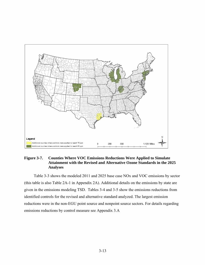
3-13
Figure 3-7. Counties Where VOC Emissions Reductions Were Applied to Simulate Attainment with the Revised and Alternative Ozone Standards in the 2025 Analyses
Table 3-3 shows the modeled 2011 and 2025 base case NOx and VOC emissions by sector
(this table is also Table 2A-1 in Appendix 2A). Additional details on the emissions by state are
given in the emissions modeling TSD. Tables 3-4 and 3-5 show the emissions reductions from
identified controls for the revised and alternative standard analyzed. The largest emission
reductions were in the non-EGU point source and nonpoint source sectors. For details regarding
emissions reductions by control measure see Appendix 3.A

3-14
Table 3-3. 2011 and 2025 Base Case NOx and VOC Emissions by Sector (1000 tons) Sector 2011 NOx 2025 NOx 2011 VOC 2025 VOC
EGU-point 2,000 1,400 36 42 NonEGU-point 1,200 1,200 800 830
Point oil and gas 500 460 160 190 Wild and Prescribed Fires 330 330 4,700 4,700
Nonpoint oil and gas 650 720 2,600 3,500 Residential wood
combustion 34 35 440 410
Other nonpoint 760 790 3,700 3,500 Nonroad 1,600 800 2,000 1,200 Onroad 5,700 1,700 2,700 910
C3 Commercial marine vessel (CMV)
130 100 5 9
Locomotive and C1/C2 CMV
1,100 680 48 24
Biogenics 1,000 1,000 41,000 41,000 TOTAL 15,000 9,300 58,000 56,000
Table 3-4. Summary of Emissions Reductions by Sector for the Identified Control Strategies Applied for the Revised 70 ppb Ozone Standard in 2025, except California (1,000 tons/year)a
Geographic Area Emissions Sector NOx VOC
East
EGU 45 - Non-EGU Point 85 1 Nonpoint 100 19 Nonroad 3 - Onroad - - Total 230 20
West
EGU - - Non-EGU Point 6 - Nonpoint 1 - Nonroad - - Onroad - - Total 7 -
a Emissions reduction estimates are rounded to two significant figures.

3-15
Table 3-5. Summary of Emissions Reductions by Sector for the Identified Control Strategies for the Alternative 65 ppb Ozone Standard in 2025 - except California (1,000 tons/year)a
Geographic Area Emissions Sector NOx VOC
East
EGU 110 - Non-EGU Point 220 5 Nonpoint 160 100 Nonroad 8 - Total 500 100
West
EGU 0 - Non-EGU Point 33 - Nonpoint 22 5 Nonroad 1 - Total 56 5
a Emissions reduction estimates are rounded to two significant figures.
As mentioned previously, there were several areas where identified controls did not
achieve enough emissions reductions to meet the revised and alternative standards of 70 and 65
ppb. Texas East was the only area where identified controls were not enough to get the needed
emissions reductions for 70 ppb. Great Lakes, Colorado, Texas East, Ohio River Valley,
Northeast and Nevada were the areas where identified controls were not enough to get the
needed emissions reductions for 65 ppb. See Chapter 2, Figure 2-2 for a map showing these
areas. To complete the analysis, the EPA then assumed that the remaining reductions needed to
meet the standard would be obtained from unidentified controls. Table 3-6 shows the emissions
reductions needed from unidentified controls in 2025 for the U.S., except California, for the
revised and alternative standards analyzed.
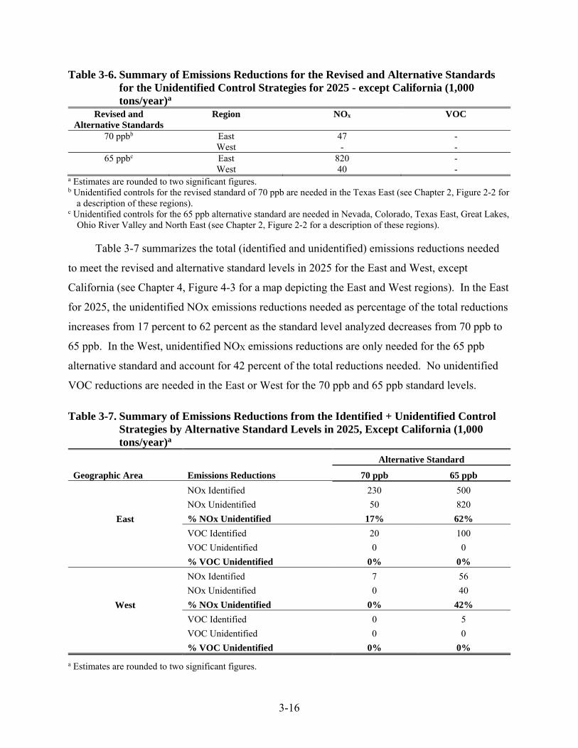
3-16
Table 3-6. Summary of Emissions Reductions for the Revised and Alternative Standards for the Unidentified Control Strategies for 2025 - except California (1,000 tons/year)a
Revised and Alternative Standards
Region NOx VOC
70 ppbb East West
47 -
- -
65 ppbc East West
820 40
- -
a Estimates are rounded to two significant figures. b Unidentified controls for the revised standard of 70 ppb are needed in the Texas East (see Chapter 2, Figure 2-2 for
a description of these regions). c Unidentified controls for the 65 ppb alternative standard are needed in Nevada, Colorado, Texas East, Great Lakes,
Ohio River Valley and North East (see Chapter 2, Figure 2-2 for a description of these regions).
Table 3-7 summarizes the total (identified and unidentified) emissions reductions needed
to meet the revised and alternative standard levels in 2025 for the East and West, except
California (see Chapter 4, Figure 4-3 for a map depicting the East and West regions). In the East
for 2025, the unidentified NOx emissions reductions needed as percentage of the total reductions
increases from 17 percent to 62 percent as the standard level analyzed decreases from 70 ppb to
65 ppb. In the West, unidentified NOX emissions reductions are only needed for the 65 ppb
alternative standard and account for 42 percent of the total reductions needed. No unidentified
VOC reductions are needed in the East or West for the 70 ppb and 65 ppb standard levels.
Table 3-7. Summary of Emissions Reductions from the Identified + Unidentified Control Strategies by Alternative Standard Levels in 2025, Except California (1,000 tons/year)a
Alternative Standard
Geographic Area Emissions Reductions 70 ppb 65 ppb
East
NOx Identified 230 500
NOx Unidentified 50 820
% NOx Unidentified 17% 62%
VOC Identified 20 100
VOC Unidentified 0 0
% VOC Unidentified 0% 0%
West
NOx Identified 7 56
NOx Unidentified 0 40
% NOx Unidentified 0% 42%
VOC Identified 0 5
VOC Unidentified 0 0
% VOC Unidentified 0% 0%
a Estimates are rounded to two significant figures.

3-17
3.2 The Post-2025 Scenario for California
The post-2025 baseline and alternative standard level scenarios for California were created
using similar methods to those described above in Section 3.1. However, in contrast to the rest
of the U.S., substantial emissions reductions were needed in California to meet the current
standard of 75 ppb. All identified controls were used to meet the current standard in this process,
so the revised and alternative standards analyzed in California relied entirely on unidentified
measures.
3.2.1 Creation of the Post-2025 Baseline Scenario for California
The final 2025 base case projections predict several areas of California would have ozone
DVs above the current standard level of 75 ppb. Therefore, we estimated emissions reductions
in the following order to construct the post-2025 baseline scenario for California: (1) emissions
changes from the Clean Power Plan, (2) mobile source emissions changes between 2025 and
2030, (3) identified controls of NOx emissions from nonpoint, non-EGU point, and nonroad
sources, (4) identified controls of VOC emissions, and (5) additional NOx reductions beyond
identified controls (i.e., unidentified controls). All controls applied to these sources were above
and beyond reductions from on-the-books regulations that were included in the final 2025 base
case modeling. The following paragraphs and Figure 3-8 outline these steps.
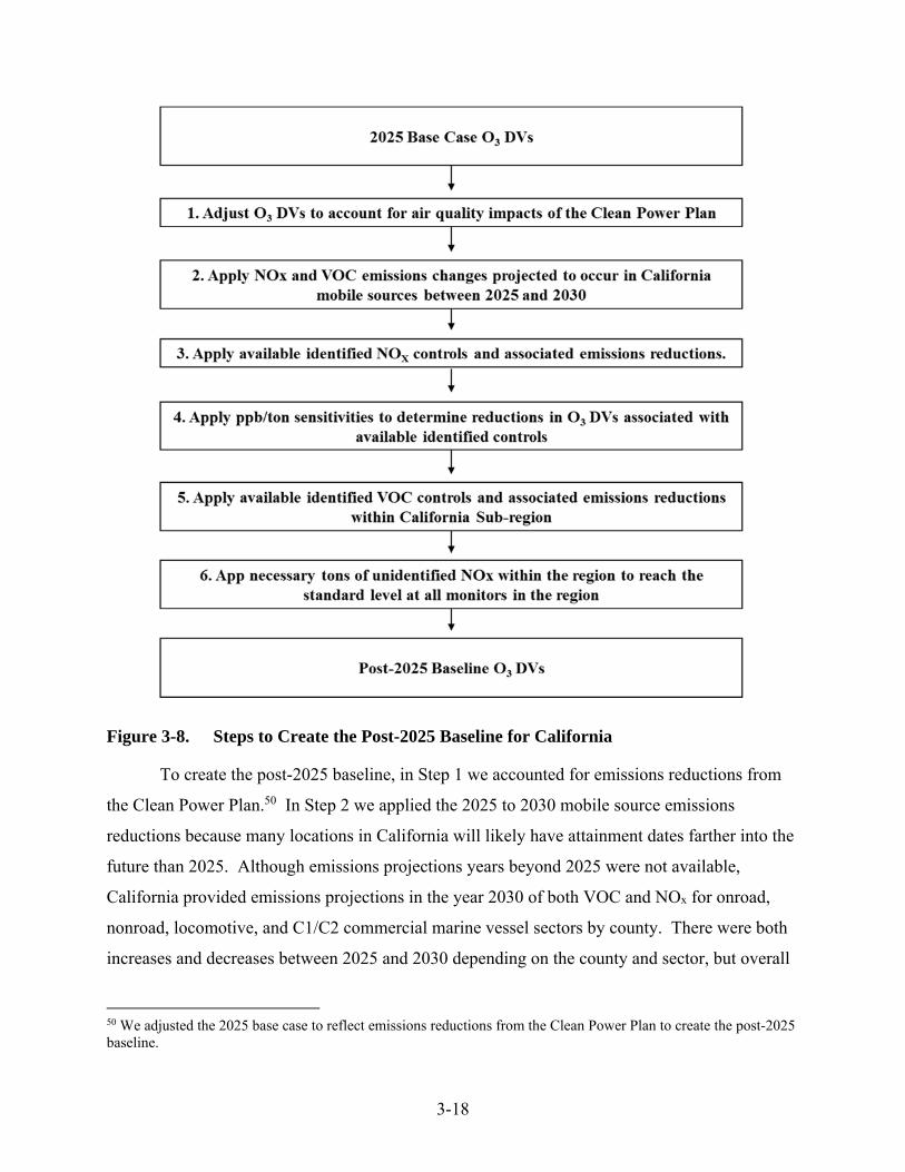
3-18
Figure 3-8. Steps to Create the Post-2025 Baseline for California
To create the post-2025 baseline, in Step 1 we accounted for emissions reductions from
the Clean Power Plan.50 In Step 2 we applied the 2025 to 2030 mobile source emissions
reductions because many locations in California will likely have attainment dates farther into the
future than 2025. Although emissions projections years beyond 2025 were not available,
California provided emissions projections in the year 2030 of both VOC and NOx for onroad,
nonroad, locomotive, and C1/C2 commercial marine vessel sectors by county. There were both
increases and decreases between 2025 and 2030 depending on the county and sector, but overall
50 We adjusted the 2025 base case to reflect emissions reductions from the Clean Power Plan to create the post-2025 baseline.
3-19
these mobile source changes resulted in: (1) VOC emissions that were 1% less than those
modeled in the California base case in both the Northern and Southern California sub-regions
(see Chapter 2, Figure 2-2 for a depiction of the California sub-regions), and (2) NOx emissions
that were 4% less than those modeled in the California base case in the Northern California sub-
region and 3% less than those modeled in the Southern California sub-region. The NOx and
VOC mobile source emissions changes were applied to create the post-2025 baseline scenario in
California using the response ratios developed from the air quality sensitivity simulations as
described in Chapter 2. In Step 3 available NOx reductions from identified control measures
were applied from three sectors:51 Non-Electric Generating Unit Point Sources (Non-EGUs),
Nonpoint (Area) Sources, and Nonroad Mobile Sources. No controls for EGUs within the
parameters of size (25 tpy) and dollar per ton control costs less than $19,000 per ton were
available for California. Table 3-1 above also includes identified controls that we applied in
California. In Step 4, the ppb/ton from the sensitivities were applied to determine ozone
reductions. Then, in Step 5, VOC controls were applied in the California counties indicated in
Figure 3-10.
In Step 6, we used additional reductions (assumed to come from unidentified NOX
controls) in Southern California and associated regional ppb/ton response factors from the
Southern California combined sensitivity simulations to reduce DVs at Southern California
monitors to reach the current standard of 75 ppb. As described in Chapter 2 and shown in the
example calculation in Appendix 3-A, we applied emissions responses derived from multiple
emissions sensitivity simulations to capture the nonlinear response of large emissions reductions
in Southern California. Similarly, we used unidentified reductions and associated ppb/ton
response factors from Northern California to reduce DVs at Northern California monitors. Since
the highest projected DVs occurred in Southern California, we first quantified necessary
emissions reductions from unidentified NOx reduction measures to reduce all Southern
California monitors to 75 ppb or lower. We then recalculated the resulting Northern California
DVs before determining how many additional emissions reductions from unidentified NOx
51 In establishing the baseline, the U.S. EPA selected a set of cost-effective controls to simulate attainment of the
current ozone standard. These control sets are hypothetical because states will ultimately determine controls as part of the SIP process.

3-20
control measures in Northern California would be necessary to bring all Northern California
monitors into attainment with the current standard of 75 ppb. Summaries of the emissions
reductions are presented for the post-2025 baseline in Appendix 3A. The resulting ozone DVs at
all evaluated monitors are also provided in Appendix 2A, Section 2A.4.
The post-2025 baseline for this analysis presents one scenario of future year air quality
based upon specific control measures, additional emissions reductions beyond identified
controls, promulgated federal rules such as Tier 3, and specific years of initial values for air
quality monitoring and emissions data. This analysis presents one illustrative approach relying
on the identified federal measures and other strategies that states may employ. California may
ultimately employ other strategies and/or other federal rules may be adopted that would also help
in achieving attainment with the current standard.
3.2.2 Approach for Revised Standard of 70 ppb and Alternative Standard of 65 ppb for California
We created the post-2025 70 ppb and 65 ppb scenarios by applying emissions reductions
incrementally to the post-2025 baseline. As mentioned above, all identified measures in
California were exhausted in reaching the post-2025 baseline. We started with the post-2025
baseline and then applied NOx from unidentified controls to meet the revised and alternative
standard levels. As with the baseline, we first identified the NOx reductions in Southern
California that would be required to bring Southern California monitors down to the revised and
alternative standard levels. We then recalculated the Northern California DVs that would result
from the Southern California emissions reductions and applied additional Northern California
unidentified NOx emissions reductions to bring all Northern California monitors down to the
revised and alternative standard levels. Also, as was done for the baseline, we applied ppb/ton
response levels that were derived from multiple emissions sensitivities to capture nonlinear
responses of ozone to large emissions reductions in California (see example calculation in
Appendix 3-A).
3.2.3 Results for California
Nine counties in California were projected to exceed the current ozone standard of 75 ppb
in the post-2025 baseline scenario (see Figure 3-9). Figure 3-10 shows areas where identified

3-21
control measures were applied to bring ozone DVs in those counties into attainment with the
current standard and establish the baseline. Table 3-8 includes a summary of NOx and VOC
emissions reductions needed to demonstrate attainment of the current ozone standard of 75 ppb.
Figure 3-9. Counties Projected to Exceed 75 ppb in the Post-2025 Baseline Scenario

3-22
Figure 3-10. Counties Where Emissions Reductions Were Applied to Demonstrate Attainment with the Current Standard
Table 3-8. Summary of Emissions Reductions (Identified + Unidentified Controls) Applied to Demonstrate Attainment in California for the Post-2025 Baseline (1,000 tons/year)a
Emissions Sector NOx VOC
Identified Controls
EGU - - Non-EGU Point 14 1 Nonpoint 14 54 Nonroad 4 - Onroad - - Total 32 55
Unidentified Controls All 160 - Total 190 55 Percent Unidentified 84% 0%
a Emission reduction estimates are rounded to two significant figures.
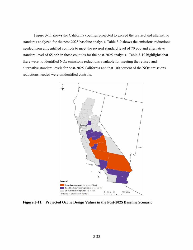
3-23
Figure 3-11 shows the California counties projected to exceed the revised and alternative
standards analyzed for the post-2025 baseline analysis. Table 3-9 shows the emissions reductions
needed from unidentified controls to meet the revised standard level of 70 ppb and alternative
standard level of 65 ppb in those counties for the post-2025 analysis. Table 3-10 highlights that
there were no identified NOx emissions reductions available for meeting the revised and
alternative standard levels for post-2025 California and that 100 percent of the NOx emissions
reductions needed were unidentified controls.
Figure 3-11. Projected Ozone Design Values in the Post-2025 Baseline Scenario

3-24
Table 3-9. Summary of Emissions Reductions from Unidentified Control Strategy for the Revised and Alternative Standard Levels for Post-2025 - California (1,000 tons/year)a
Alternative Standard Region NOx VOC 70 ppb CA 51 - 65 ppb CA 100 -
a Estimates are rounded to two significant figures.
Table 3-10. Summary of Emissions Reductions from the Identified + Unidentified
Control Strategy by the Revised and Alternative Standard Levels for Post-2025 - California (1,000 tons/year)a
Alternative Standard Geographic Area Emissions Reductions 70 ppb 65 ppb
California
NOx Identified 0 0 NOx Unidentified 51 100 % NOx Unidentified 100% 100% VOC Identified 0 0 VOC Unidentified 0 0 % VOC Unidentified 0% 0%
a Estimates are rounded to two significant figures.
3.3 Improvements and Refinements since the Proposal RIA
In the regulatory impact analyses for both the ozone NAAQS proposal and final, there
were two geographic areas outside of California where the majority of emissions reductions were
needed to meet an alternative standard level of 70 ppb – Texas and the Northeast. In analyzing
the revised standard of 70 ppb for the final RIA, there were approximately 50 percent fewer
emissions reductions needed in these two areas. For an alternative standard of 65 ppb, emissions
reductions needed nationwide were approximately 20 percent lower than at proposal.
The primary reason for the difference in emissions reductions needed for both 70 and 65
ppb is that in the final RIA we conducted more geographically-refined air quality sensitivity
modeling to develop improved response factors (i.e., changes in ozone concentrations in
response to emissions reductions). More detailed air quality modeling and improved response
factors account for 80 percent of the difference in needed emissions reductions between proposal
and final. See Chapter 2, Section 2.4.2 for a discussion of the air quality modeling.
For the analysis of the revised standard of 70 ppb, in Texas and the Northeast, the
improved and refined response factors and more geographically focused emissions reductions

3-25
strategies resulted in larger changes in ozone concentrations. In east Texas, the ppb/ton response
factors used in the final RIA were 2 to 3 times more responsive than the factors used in the
proposal RIA at controlling monitors in Houston and Dallas. In the Northeast, the ppb/ton
response factors used in the final RIA were 2.5 times more responsive than the factors used in
the proposal RIA at the controlling monitor on Long Island, NY.
A secondary reason for the difference is that between the proposal and final RIAs we
updated models and model inputs for the base year of 2011. See Appendix 2, Section 2A.1.3 for
additional discussion of the updated models and model inputs. When projected to 2025, these
changes in models and inputs had compounding effects for year 2025, and in some areas resulted
in lower projected base case design values for 2025. In these areas, the difference between the
base case design values and a standard of 70 ppb was smaller, thus requiring fewer emissions
reductions to attain the 70 ppb revised standard.
Note that the more spatially refined emissions sensitivity modeling had more impact on the
results at 70 ppb than it did on the results at 65 ppb due to the more localized nature of projected
exceedances at 70 ppb. For example, as described above, the new sensitivity regions showed
that emissions reductions in eastern Texas would have a larger impact on ozone in Houston and
Dallas than the same emissions reductions would have if they were spread over the central U.S.
states used in the proposal RIA. Conversely, these same east Texas emissions reductions would
have less impact on violating monitors in Louisiana or Oklahoma. Therefore, for the 65 ppb
scenario, additional local controls were necessary in Louisiana and Oklahoma.
As a consequence of the use of more geographically refined sensitivity regions, emissions
reductions control strategies were also applied in geographic areas closer to the monitors of
projected exceedances. For example, in the proposal RIA, the Central region included Texas,
Oklahoma, Kansas, Missouri, Arkansas, Louisiana and Mississippi, meaning that controls could
be applied anywhere in those states after identified controls had been exhausted within the 200
km buffer. But in the final RIA, the only geographic area where we applied controls was East
Texas. Thus, once identified control measures were exhausted there, we had to obtain remaining
reductions from unidentified control measures. While the total amount of emissions needed to

3-26
meet the 65 ppb alternative standard is lower than it was in the proposal RIA, the fraction of
emissions reductions from identified controls was smaller.
3.4 Limitations and Uncertainties
EPA’s analysis is based on its best judgment for various input assumptions that are
uncertain. As a general matter, the Agency selects the best available information from
engineering studies of air pollution controls and has set up what it believes is the most reasonable
modeling framework for analyzing the cost, emissions changes, and other impacts of regulatory
controls. However, the control strategies above are subject to important limitations and
uncertainties. In the following, we discuss the limitations and uncertainties that are most
significant.
Illustrative control strategy: A control strategy is the set of actions that States
may take to meet a standard, such as which industries should be required to install
end-of-pipe controls or certain types of equipment and technology. The illustrative
control strategy analysis in this RIA presents only one potential pathway to
attainment. The control strategies are not recommendations for how a revised ozone
standard should be implemented, and States will make all final decisions regarding
implementation strategies for the revised NAAQS. We do not presume that the
control strategies presented in this RIA are an exhaustive list of possibilities for
emissions reductions.
Emissions inventories and air quality modeling: These serve as a foundation for
the projected ozone values, control strategies and costs in this analysis and thus
limitations and uncertainties for these inputs impact the results, especially for
issues such as future year emissions projections and information on controls
currently in place at sources. Limitations and uncertainties for these inputs are
discussed in previous chapters devoted to these subject areas. In addition, there are
factors that affect emissions, such as economic growth and the makeup of the
economy (e.g., growth in the oil and natural gas sector), that introduce additional
uncertainty.

3-27
Projecting level and geographic scope of exceedances: Estimates of the
geographic areas that would exceed revised alternative levels of the standard in a
future year, and the level to which those areas would exceed, are approximations
based on a number of factors. The actual nonattainment determinations that would
result from a revised standard will likely depend on the consideration of local
issues, changes in source operations between the time of this analysis and
implementation of a new standard, and changes in control technology over time.
Assumptions about the baseline: There is significant uncertainty about the
illustration of the impact of rules, especially the Clean Power Plan because there is
significant flexibility for states to determine which measures to apply to comply
with the standard.
Sequential processing of regional emission reductions: Because this method
prioritizes emissions reductions in the regions with the highest ozone values first
but then does not go back and re-evaluate the amount of reduction in the higher
priority region after emissions reductions have been applied in lower-priority
regions, there is the potential to reduce a greater quantity of emissions at monitors
in the higher priority regions. For instance, in the 65 ppb scenario, in the
Northeast, the monitor which required the largest emissions reductions to reach 65
ppb was located in Queens, NY. After identifying necessary emissions reductions
in the Northeast region, that monitor had a projected DV of 65.996 ppb (which
truncates to 65 ppb). Additional reductions from lower priority regions such as the
Ohio River Valley and the Great Lakes, brought the DV at that site down to 65.002
ppb. In theory, fewer tons of emissions reductions could then have been applied in
the Northeast to reach a DV less than 66 ppb. However, if emissions reductions in
the Northeast were rolled back, then necessary reductions in all lower priority
regions would need to be recalculated and consequently the degree to which the
Northeast emissions reductions were rolled back would also need to be
recalculated. This could be quantified either in an iterative process or through a
linear programming model that found a least cost solution based on all response
factors and associated costs. Neither of these options were available for this
analysis, but it should be noted that this likely leads to some overestimate in our

3-28
calculation of tons of emissions reductions necessary to meet the 70 and 65 ppb
standard levels and in the resulting costs and benefits.
Applicability of control measures: The applicability of a control measure to a
specific source varies depending on a number of process equipment factors such as
age, design, capacity, fuel, and operating parameters. These can vary considerably
from source to source and over time. This analysis makes assumptions across broad
categories of sources nationwide.
Control measure advances over time: As we focus on the advances that might be
expected in existing pollution control technologies, we recognize that the control
measures applied do not reflect potential effects of technological change that may
be available in future years. The effects of “learning by doing” or “learning by
researching” are not accounted for in the emissions reduction estimates. Thus, all
estimates of impacts associated with control measures applied reflect our current
knowledge, and not projections, of the measures’ effectiveness or costs. In our
analysis, we do not have the necessary data for cumulative output, fuel sales, or
emissions reductions for all sectors included in order to properly generate control
costs that reflect learning-curve impacts or the impacts of technological change. We
believe the effect of including these impacts may change our estimates of costs for
our projected year control strategies.
Pollutants to be targeted: Local knowledge of atmospheric chemistry in each
geographic area may result in a different prioritization of pollutants (VOC and
NOx) for control. For the baseline in this analysis, we included only promulgated
or proposed rules, but that there may be additional regulations promulgated in the
future that reduce NOx or VOC emissions (see Chapter 4, Section 4.2 for additional
discussion of the Phase 2 Heavy Duty Greenhouse Gas Standards for New Vehicles
and Engines). These regulations could reduce the current baseline levels of
emissions.

3-29
3.5 References
U.S. Environmental Protection Agency (U.S. EPA). User’s Guide for the Final NONROAD 2005 Model. Available at http://www.epa.gov/otaq/models/nonrdmdl/nonrdmdl2005/420r05013.pdf.
U.S. Environmental Protection Agency (U.S. EPA). 2014a. Control of Air Pollution from Motor Vehicles: Tier 3 Motor Vehicle Emission and Fuel Standards. Office of Transportation and Air Quality. Available at http://www.epa.gov/otaq/tier3.htm.
U.S. Environmental Protection Agency (U.S. EPA). 2014b. Control Strategy Tool (CoST) Documentation Report. Office of Air Quality Planning and Standards, Research Triangle Park, NC. Available at http://www.epa.gov/ttnecas1/cost.htm.U.S. Environmental Protection Agency (U.S. EPA). 2015. EPA Base Case v.5.14 Using the Integrated Planning Model, Incremental Documentation. Available at http://www.epa.gov/airmarkets/documents/ipm/EPA_Base_Case_v514_Incremental_Documentation.pdf

3A-1
APPENDIX 3A: CONTROL STRATEGIES AND EMISSIONS REDUCTIONS
Overview
Chapter 3 describes the approach that EPA used in applying control measures to
demonstrate attainment of alternative ozone standard levels of 70. This Appendix contains more
detailed information about the control strategy analyses, including numerical examples of the
calculation methods for changes in ozone DVs, the control measures that were applied and the
geographic areas in which they were applied.
3A.1 Target Emissions Reductions Needed to Create the Baseline, Post-2025 Baseline and Alternatives
Tables 3A-1 to 3A-3 depict emissions reductions required in each region to reach the
alternative standard level scenarios for the U.S. except California, and the post-2025 Baseline
and alternative standard levels for California. These emissions reductions were determined using
the methodology described in Chapter 3, Sections 3.1 and 3.2 and illustrated in the numerical
example in section 3A.2 of this Appendix. Sector-specific controls used for these reductions are
discussed in more detail in Chapter 3. These emissions reductions were used to create the ozone
surfaces described in Chapter 2, Section 2.4.

3A-2
Table 3A-1. Emissions Reductions Applied Beyond the Baseline Scenario to Create the 70 ppb Scenario
Emissions reductions (thousand tons) applied from
NOx reductions from
identified controls VOC reductions from
identified controls
Additional NOx reductions from
unidentified measures Northeast 111 - - Ohio River Valley 27 - - Great Lakes 18 - - East Texas 123 20 (Houston) - Colorado 7 - -
N. California Exhausted in baseline
scenario Exhausted in baseline
scenario 35
S. California Exhausted in baseline
scenario Exhausted in baseline
scenario 16
Table 3A-2. Emissions Reductions Applied Beyond the Baseline Scenario to Create the 65
ppb Scenario Emissions reductions (thousand tons) applied from
NOx reductions from
identified controls VOC reductions from
identified controls
Additional NOx reductions from
unidentified measures Northeast 163 41 (NY area) 285
Ohio River Valley 169 7 (Louisville area) 112 Great Lakes 197 39 (Chicago area) 56 OK/AR/LA 24 - -
E. Texas 123 20 (Houston area) 188 AZ/NM 29 - - Colorado 36 5 (Denver area) 20 Nevada 10 - -
N. California Exhausted in baseline
scenario Exhausted in baseline
scenario 65.5
S. California Exhausted in baseline
scenario Exhausted in baseline
scenario 32
Table 3A-3. Emissions Reductions Applied to Create the Post-2025 Baseline Scenario* Emissions reductions (thousand tons) applied from
2025-2030 California
mobile source changes
NOx reductions from identified
controls
VOC reductions from identified
controls
Additional NOx reductions from
unidentified measures
N. California 8 (NOx) 3 (VOC)
16 27 24
S. California 6 (NOx) 3 (VOC)
16 29 136
*These emission are in addition to changes modeled in the simulation representing option 1(state) of the proposed carbon pollution guidelines under section 111(d) of the CAA.

3A-3
3A.2 Numeric Examples of Calculation Methodology for Changes in Design Values
In this section we use the data for two monitoring sites to demonstrate how changes in
design values were calculated, as described in Sections 3.1 and 3.2. For each monitor, numerical
examples are given for calculating the emissions reductions necessary to attain the current
standard of 75 ppb (i.e., the baseline scenario) as well as the 70 ppb scenario, which is
incremental to the baseline. Note that design values are truncated when they are compared to a
standard level, so a calculated design value of 75.9 is truncated to 75 ppb and, therefore, meets
the current 75 ppb standard. Similarly, a design value of 70.9 would meet an alternative standard
level of 70. For each monitor, we start with the base case design value, then account for ozone
changes simulated in the 111(d) sensitivity simulation and then apply equation 2-5 from Chapter
2.
, , ∆ , ∆ , ∆ ⋯ Eq 2-5
Example 1. Fresno California monitor 60195001 (baseline):
,
83.4,
0.7∆ ,
5.0 10,
32,000∆
1.4 10, ,
8000 24,000∆ , ∆
9.9 10, _ ,
3000 27,000∆ , ∆
2.3 10, ,
6000 100,000∆ , ∆
2.6 10, ,
36,000∆
75.9

3A-4
Example 2. Fresno California monitor 60195001 (65 ppb scenario):
, 75.9,
1.4 10, ,
35,000∆
%
2.6 10, ,
16,000∆
70.9
Example 3. Dallas monitor 484392003 (baseline):
, 74.3,
1.0∆ ,
73.3
Example 4. Dallas monitor 484392003 (65 ppb scenario):
, 73.3,
3.3 10, .
123,000∆
4.1 10,
111,000∆
5.1 10,
7000∆
2.6 10,
27,000∆
1.9 10,
18,000∆
69.3
3A.3 Types of Control Measures
Several types of control measures were applied in the analyses for the baseline and alternative standard levels. These can be grouped into the following classes:

3A-5
NOx Reductions – NOx control measures for nonEGU point, nonpoint, and nonroad sources. For each of these sources, we identified the most effective control (i.e., control with the highest percent reduction) that could be applied to the source, given the following constraints:
the source must emit at least 25 tons/yr of NOx (see description of controls on smaller sources below);
any control for nonEGU sources must result in a reduction of NOx emissions of at least 5 tons/yr; and
any replacement control (i.e., a more effective control replacing an existing control) must achieve at least 10% more reduction than the existing control (e.g., we would not replace a 60% control with a 65% control).
NOx Reductions from EGU SCRs and SNCRs – applied to coal-fired EGUs where they are in place but are idle.
VOC Reductions – VOC control measures for nonEGU and nonpoint sources that:
emit at least 10 tons/yr of VOC;
any control must result in a reduction of VOC of at least 1 ton/yr; and
any replacement control must achieve 10% more reduction than the existing control.
3A.4 Application of Control Measures in Geographic Areas
Control measures were applied, to obtain the emissions reductions described in Section
3A.1 of this Appendix, to geographic areas including or adjacent to areas that were projected to
exceed the baseline and alternative standards. If all non-EGU NOx reductions were needed, then
the maximum emissions reductions algorithm in CoST was used. Where less non-EGU NOx
reductions were needed than were available, these were obtained using the least cost algorithm.
Where VOC reductions were needed, all potentially available VOC reductions were needed so
these were identified using the maximum emissions reduction algorithm. No unidentified
controls were needed for VOC emissions reductions. Tables 3A-4 and 3A-5 show where
controls were applied and where unidentified controls were needed in the U.S. except California.
Tables 3A-6 and 3A-7 show where controls were applied and where unidentified controls were
needed in California.

3A-6
Table 3A-4. Geographic Areas for Application of NOx Controls in the Baseline and Alternative Standard Analyses - U.S., except Californiaa
Geographic Areas and Controls Baseline 70 ppb 65 ppb
EAST
North East
Inside buffer
Non-EGU x x EGU x x
Outside buffer x x Unidentified U
OK + AR + LA
Inside buffer
Non-EGU x EGU
Outside buffer
Unidentified
Ohio River Valley
Inside buffer
Non-EGU x x EGU x x
Outside buffer x x Unidentified U
TX East
Inside buffer
Non-EGU x x EGU
Outside buffer x x Unidentified U U
WEST
AZ + NM
Inside buffer
Non-EGU x EGU
Outside buffer x Unidentified
Colorado
Inside buffer
Non-EGU x x EGU
Outside buffer x Unidentified U

3A-7
Geographic Areas and Controls Baseline 70 ppb 65 ppb Great Lakes
Inside buffer
Non-EGU x x EGU x
Outside buffer x x Unidentified U
Nevada
Inside buffer
Non-EGU x EGU
Outside buffer x
Unidentified U
a “x” indicates known controls were applied; “U” indicates unknown control reductions.
Table 3A-5. Geographic Areas for Application of VOCa Controls in the Baseline and Alternative Standard Analyses - U.S., except Californiab
Geographic Area Baseline 70 ppb 65 ppb
EAST x
North East
New York, New Jersey, Long Island, NY-NJ-CT
Ohio River Valley
Louisville, KY x
TX East
Houston-Galveston-Brazoria, TX x x
WEST
Colorado
Denver-Boulder-Greeley-Ft.Collins-Loveland, CO x
Great Lakes
Chicago-Lake Michigan, WI-IL-IN-MI x
a No unidentified VOC controls were needed to attain any of the standards; b “x” indicates known controls were
applied

3A-8
Table 3A-6. Geographic Areas for Application of NOxa Controls in the Baseline and
Alternative Standard Analyses – Californiab Geographic Areas and Control Groups Baseline 70 ppb 65 ppb
California California North Identified x California North Unidentified U U U California South Identified x California South Unidentified U U U
a All reductions were calculated using the maximum reductions algorithm b “x” indicates known controls were
applied; “U” indicates unknown control reductions.
Table 3A-7. Geographic Areas for Application of VOCa Controls in the Baseline and Alternative Standard Analyses – Californiab
Geographic Areas and Control Groups Baseline 70 ppb 65 ppb
California California North – San Joaquin x Identified U U U Unidentified California South – Los Angeles Identified x Unidentified U U U
a All reductions were calculated using the maximum reductions algorithm b “x” indicates known controls were
applied; “U” indicates unknown control reductions.
3A.5 NOx Control Measures for Non-EGU Point Sources
Several types of NOx control technologies exist for non-EGU point sources: selective
catalytic reduction (SCR), selective noncatalytic reduction (SNCR), natural gas reburn (NGR),
coal reburn, and low-NOx burners (LNB). In some cases, LNB accompanied by flue gas
recirculation (FGR) is applicable, such as when fuel-borne NOx emissions are expected to be of
greater importance than thermal NOx emissions. When circumstances suggest that combustion
controls do not make sense as a control technology (e.g., sintering processes, coke oven batteries,
sulfur recovery plants), SNCR or SCR may be an appropriate choice. Finally, SCR can be
applied along with a combustion control such as LNB with overfire air (OFA) to further reduce
NOx emissions. All of these control measures are available for application on industrial boilers.
Besides industrial boilers, other non-EGU point source categories covered in this RIA
include petroleum refineries, kraft pulp mills, cement kilns, stationary internal combustion
engines, glass manufacturing, combustion turbines, and incinerators. NOx control measures

3A-9
available for petroleum refineries, particularly process heaters at these plants, include LNB,
SNCR, FGR, and SCR along with combinations of these technologies. NOx control measures
available for kraft pulp mills include those available to industrial boilers, namely LNB, SCR,
SNCR, along with water injection. NOx control measures available for cement kilns include
those available to industrial boilers, namely LNB, SCR, and SNCR. Non-selective catalytic
reduction (NSCR) can be used on stationary internal combustion engines. OXY-firing, a
technique to modify combustion at glass manufacturing plants, can be used to reduce NOx at
such plants. LNB, SCR, and SCR plus steam injection (SI) are available measures for
combustion turbines. Finally, SNCR is an available control technology at incinerators.
Tables 3A-8 through 3A-11 contain lists of the NOx and VOC control measures applied
in these analyses for non-EGU point sources, EGUs, nonpoint sources, and nonroad sources. The
table also presents the associated emission reductions for the baseline and alternative standard
analyses. The number of geographic areas in which they were applied expanded as the level of
the alternative standard analyzed became more stringent.
Table 3A-8. NOx Control Measures Applied in the 70 ppb Analysis NOx Control Measure Reductions (tons/year)
Adjust Air to Fuel Ratio and Ignition Retard - Gas Fired IC Engines 8,723
Biosolid Injection Technology - Cement Kilns 5,383
EGU SCR & SNCR 44,951
Episodic Burn Ban 2,797
Excess O3 Control 229
Ignition Retard - IC Engines 618
Low Emission Combustion - Gas Fired Lean Burn IC Engines 17,676
Low NOx Burner - Coal Cleaning 270
Low NOx Burner - Commercial/Institutional Boilers & IC Engines 21,417
Low NOx Burner - Gas-Fired Combustion 9,237
Low NOx Burner - Glass Manufacturing 247
Low NOx Burner - Industr/Commercial/Institutional (ICI) Boilers 5,580
Low NOx Burner - Industrial Combustion 25
Low NOx Burner - Lime Kilns 2,433
Low NOx Burner - Natural Gas-Fired Turbines 6,276
Low NOx Burner - Residential Water Heaters & Space Heaters 19,900
Low NOx Burner and Flue Gas Recirculation - Coke Oven/Blast Furnace 359
Low NOx Burner and Flue Gas Recirculation - Fluid Catalytic Cracking Units 84
Low NOx Burner and Flue Gas Recirculation - Iron & Steel 399
Low NOx Burner and SCR - Industr/Commercial/Institutional Boilers 8,408
Mid-Kiln Firing - Cement Manufacturing 1,241
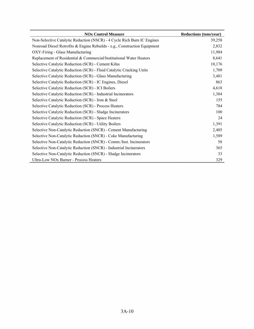
3A-10
NOx Control Measure Reductions (tons/year)
Non-Selective Catalytic Reduction (NSCR) - 4 Cycle Rich Burn IC Engines 39,258
Nonroad Diesel Retrofits & Engine Rebuilds - e.g., Construction Equipment 2,832
OXY-Firing - Glass Manufacturing 11,984
Replacement of Residential & Commercial/Institutional Water Heaters 8,641
Selective Catalytic Reduction (SCR) - Cement Kilns 10,176
Selective Catalytic Reduction (SCR) - Fluid Catalytic Cracking Units 1,709
Selective Catalytic Reduction (SCR) - Glass Manufacturing 3,481
Selective Catalytic Reduction (SCR) - IC Engines, Diesel 863
Selective Catalytic Reduction (SCR) - ICI Boilers 4,618
Selective Catalytic Reduction (SCR) - Industrial Incinerators 1,384
Selective Catalytic Reduction (SCR) - Iron & Steel 155
Selective Catalytic Reduction (SCR) - Process Heaters 784
Selective Catalytic Reduction (SCR) - Sludge Incinerators 100
Selective Catalytic Reduction (SCR) - Space Heaters 24
Selective Catalytic Reduction (SCR) - Utility Boilers 1,391
Selective Non-Catalytic Reduction (SNCR) - Cement Manufacturing 2,405
Selective Non-Catalytic Reduction (SNCR) - Coke Manufacturing 1,589
Selective Non-Catalytic Reduction (SNCR) - Comm./Inst. Incinerators 58
Selective Non-Catalytic Reduction (SNCR) - Industrial Incinerators 365
Selective Non-Catalytic Reduction (SNCR) - Sludge Incinerators 33
Ultra-Low NOx Burner - Process Heaters 329

3A-11
Table 3A-9. VOC Control Measures Applied in the 70 ppb Analysis VOC Control Measure Reductions (tons/year)
Control Technology Guidelines - Wood Furniture Surface Coating 272
Control of Fugitive Releases - Oil & Natural Gas Production 9
Flare - Petroleum Flare 94
Incineration - Other 10,717
LPV Relief Valve - Underground Tanks 1,299
MACT - Motor Vehicle Coating 10
Permanent Total Enclosure (PTE) - Surface Coating 369
RACT - Graphic Arts 260
Reduced Solvent Utilization - Surface Coating 27
Reformulation - Architectural Coatings 5,246
Reformulation - Pesticides Application 171
Reformulation-Process Modification - Automobile Refinishing 220
Reformulation-Process Modification - Cutback Asphalt 655
Reformulation-Process Modification - Other 113
Reformulation-Process Modification - Surface Coating 178
Solvent Recovery System - Printing/Publishing 13
Wastewater Treatment Controls- POTWs 207

3A-12
Table 3A-10. NOx Control Measures Applied in the 65 ppb Alternative Standard Analysis NOx Control Measure Reductions (tons/year)
Adjust Air to Fuel Ratio and Ignition Retard - Gas Fired IC Engines 16,423
Biosolid Injection Technology - Cement Kilns 5,907
EGU SCR & SNCR 109,503
Episodic Burn Ban 3,283
Ignition Retard - IC Engines 575
Low Emission Combustion - Gas Fired Lean Burn IC Engines 75,724
Low NOx Burner - Coal Cleaning 475
Low NOx Burner - Commercial/Institutional Boilers & IC Engines 36,210
Low NOx Burner - Fiberglass Manufacturing 65
Low NOx Burner - Gas-Fired Combustion 11,889
Low NOx Burner - Industr/Commercial/Institutional (ICI) Boilers 21,918
Low NOx Burner - Industrial Combustion 25
Low NOx Burner - Lime Kilns 4,616
Low NOx Burner - Natural Gas-Fired Turbines 12,109
Low NOx Burner - Residential Water Heaters & Space Heaters 51,703
Low NOx Burner - Steel Foundry Furnaces 294
Low NOx Burner - Surface Coating Ovens 26
Low NOx Burner and Flue Gas Recirculation - (ICI) Boilers 477
Low NOx Burner and Flue Gas Recirculation - Coke Oven/Blast Furnace 429
Low NOx Burner and Flue Gas Recirculation - Fluid Catalytic Cracking Units 59
Low NOx Burner and Flue Gas Recirculation - Iron & Steel 781
Low NOx Burner and Flue Gas Recirculation - Process Heaters 548
Low NOx Burner and Flue Gas Recirculation - Starch Manufacturing 67
Low NOx Burner and SCR - Industr/Commercial/Institutional Boilers 24,281
Low NOx Burner and SNCR - Industr/Commercial/Institutional Boilers 482
Natural Gas Reburn - Natural Gas-Fired EGU Boilers 590
Non-Selective Catalytic Reduction (NSCR) - 4 Cycle Rich Burn IC Engines 70,008
Non-Selective Catalytic Reduction - Nitric Acid Manufacturing 491
Nonroad Diesel Retrofits & Engine Rebuilds - e.g., Construction Equipment 8,791
OXY-Firing - Glass Manufacturing 27,100
Replacement of Residential Water Heaters 133
Selective Catalytic Reduction (SCR) - Ammonia Mfg 2,336
Selective Catalytic Reduction (SCR) - Cement Kilns 26,144
Selective Catalytic Reduction (SCR) - Coke Ovens 1,243
Selective Catalytic Reduction (SCR) - Fluid Catalytic Cracking Units 4,078
Selective Catalytic Reduction (SCR) - IC Engines, Diesel 3,574
Selective Catalytic Reduction (SCR) - ICI Boilers 9,963
Selective Catalytic Reduction (SCR) - Industrial Incinerators 1,723
Selective Catalytic Reduction (SCR) - Iron & Steel 1,777
Selective Catalytic Reduction (SCR) - Process Heaters 2,744
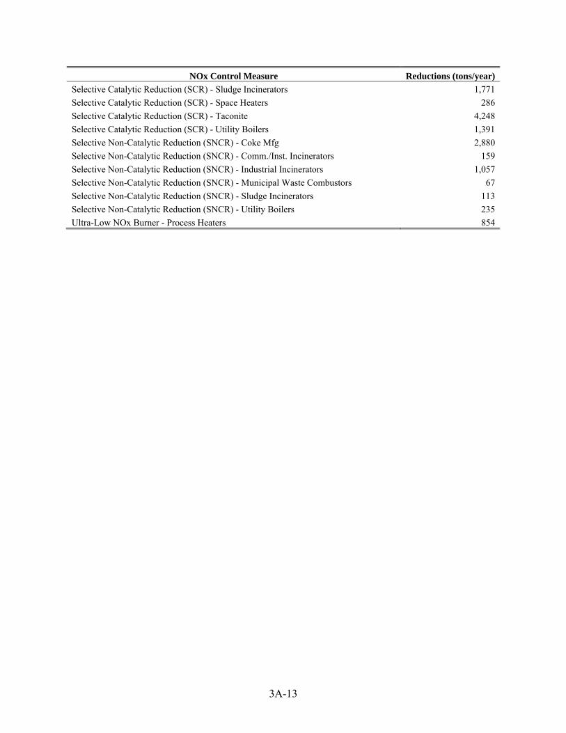
3A-13
NOx Control Measure Reductions (tons/year)
Selective Catalytic Reduction (SCR) - Sludge Incinerators 1,771
Selective Catalytic Reduction (SCR) - Space Heaters 286
Selective Catalytic Reduction (SCR) - Taconite 4,248
Selective Catalytic Reduction (SCR) - Utility Boilers 1,391
Selective Non-Catalytic Reduction (SNCR) - Coke Mfg 2,880
Selective Non-Catalytic Reduction (SNCR) - Comm./Inst. Incinerators 159
Selective Non-Catalytic Reduction (SNCR) - Industrial Incinerators 1,057
Selective Non-Catalytic Reduction (SNCR) - Municipal Waste Combustors 67
Selective Non-Catalytic Reduction (SNCR) - Sludge Incinerators 113
Selective Non-Catalytic Reduction (SNCR) - Utility Boilers 235
Ultra-Low NOx Burner - Process Heaters 854
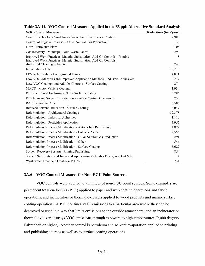
3A-14
Table 3A-11. VOC Control Measures Applied in the 65 ppb Alternative Standard Analysis VOC Control Measure Reductions (tons/year)
Control Technology Guidelines - Wood Furniture Surface Coating 2,988
Control of Fugitive Releases - Oil & Natural Gas Production 30
Flare - Petroleum Flare 108
Gas Recovery - Municipal Solid Waste Landfill 290
Improved Work Practices, Material Substitution, Add-On Controls - Printing 8 Improved Work Practices, Material Substitution, Add-On Controls -Industrial Cleaning Solvents 248
Incineration - Other 16,710
LPV Relief Valve - Underground Tanks 4,871
Low VOC Adhesives and Improved Application Methods - Industrial Adhesives 237
Low-VOC Coatings and Add-On Controls - Surface Coating 274
MACT - Motor Vehicle Coating 1,934
Permanent Total Enclosure (PTE) - Surface Coating 3,286
Petroleum and Solvent Evaporation - Surface Coating Operations 250
RACT - Graphic Arts 5,586
Reduced Solvent Utilization - Surface Coating 3,047
Reformulation - Architectural Coatings 52,378
Reformulation - Industrial Adhesives 1,110
Reformulation - Pesticides Application 3,957
Reformulation-Process Modification - Automobile Refinishing 4,879
Reformulation-Process Modification - Cutback Asphalt 2,555
Reformulation-Process Modification - Oil & Natural Gas Production 291
Reformulation-Process Modification - Other 546
Reformulation-Process Modification - Surface Coating 5,622
Solvent Recovery System - Printing/Publishing 854
Solvent Substitution and Improved Application Methods - Fiberglass Boat Mfg 14
Wastewater Treatment Controls- POTWs 234
3A.6 VOC Control Measures for Non-EGU Point Sources
VOC controls were applied to a number of non-EGU point sources. Some examples are
permanent total enclosures (PTE) applied to paper and web coating operations and fabric
operations, and incinerators or thermal oxidizers applied to wood products and marine surface
coating operations. A PTE confines VOC emissions to a particular area where they can be
destroyed or used in a way that limits emissions to the outside atmosphere, and an incinerator or
thermal oxidizer destroys VOC emissions through exposure to high temperatures (2,000 degrees
Fahrenheit or higher). Another control is petroleum and solvent evaporation applied to printing
and publishing sources as well as to surface coating operations.

3A-15
3A.7 NOx Control Measures for Nonpoint (Area) and Nonroad Sources
The nonpoint source sector of the emissions inventory is composed of sources that are
generally too small and/or numerous to estimate emissions on an individual source basis (e.g.,
dry cleaners, residential furnaces, woodstoves, fireplaces, backyard waste burning, etc). Instead,
we estimate their emissions for each county as a whole, often using an emissions factor that is
applied to a surrogate of activity such as population or number of houses.
Control measures for nonpoint sources are also applied at the county level, i.e., to the
county level emissions as a whole. Several control measures were applied to NOx emissions from
nonpoint sources. One is low NOx burner technology to reduce NOx emissions. This control is
applied to industrial oil, natural gas, and coal combustion sources. Other nonpoint source
controls include the installation of low-NOx space heaters and water heaters in commercial and
institutional sources, and episodic bans on open burning. The open burning control measure
applied to yard waste and land clearing debris. It consists of periodic daily bans on burning such
waste, as the predicted ozone levels indicate that such burning activities should be postponed.
This control measure is not applied to any prescribed burning activities.
Retrofitting diesel nonroad equipment can provide NOx and HC benefits. The retrofit
strategies included in the RIA nonroad retrofit measure are:
• Installation of emissions after-treatment devices called selective catalytic reduction
(“SCRs”)
• Rebuilding engines (“rebuild/upgrade kit”)
We chose to focus on these strategies due to their high NOx emissions reduction potential
and widespread application.
3A.8 VOC Control Measures for Nonpoint (Area) Sources
Some VOC controls for nonpoint sources are for the use of low or no VOC materials for
graphic art sources. Other controls involve the application of limits for adhesive and sealant
VOC content in wood furniture and solvent source categories. The OTC solvent cleaning rule
establishes hardware and operating requirements for specified vapor cleaning machines, as well

3A-16
as solvent volatility limits and operating practices for cold cleaners. The Low Pressure/Vacuum
Relief Valve control measure is the addition of low pressure/vacuum (LP/V) relief valves to
gasoline storage tanks at service stations with Stage II control systems. LP/V relief valves
prevent breathing emissions from gasoline storage tank vent pipes. Another control based on a
California South Coast Air Quality Management District (SQAQMD) establishes VOC content
limits for metal coatings along with application procedures and equipment requirements.
Switching to Emulsified Asphalts is a generic control measure replacing VOC-containing
cutback asphalt with VOC-free emulsified asphalt. The Reformulation control measures include
switching to and/or encouraging the use of low-VOC materials.

4-1
CHAPTER 4: ENGINEERING COST ANALYSIS AND ECONOMIC IMPACTS
Overview
This chapter provides estimates of the engineering costs of the control strategies
presented in Chapter 3 for the revised primary standard of 70 ppb and an alternative standard
level of 65 ppb and summarizes the data sources and methodologies used to estimate the
engineering costs presented in this regulatory impact analysis (RIA). As discussed in Chapter 3,
identified control measures were applied to EGU, non-EGU point, nonpoint (area), and nonroad
mobile sources to demonstrate attainment with the revised and alternative standards analyzed.52
In several areas identified controls did not achieve the emissions reductions needed to attain the
revised and alternative standards analyzed. In these areas, the EPA assumed that further controls
would be applied to reach attainment. These additional controls are referred to as unidentified
controls.
The total cost estimates include the costs of both identified and unidentified control
technologies and measures. The estimated total costs of attaining the revised and alternative
standards are partly a function of (1) assumptions used in the analysis, including assumptions
about which areas will require emissions controls and the sources and controls available in those
areas; (2) the level of sufficient, detailed information on identified control measures needed to
estimate engineering costs; and (3) the future year baseline emissions from which the emissions
reductions needed to attain are measured.
The remainder of the chapter is organized as follows. Section 4.1 presents the
engineering costs associated with the application of identified controls. Section 4.2 discusses the
challenges associated with estimating costs for unidentified controls, including a brief discussion
52 In Chapter 3, Table 3-7 lists the specific control technologies applied in the identified control measures analysis. In addition, in the proposal RIA we discuss emissions reductions resulting from the application of known controls, as well as emissions reductions beyond known controls, or in short, known controls and unknown controls. In the final RIA we refer to those sets of emissions reductions and controls as identified controls or measures and unidentified controls or measures. This terminology has been used in prior NAAQS RIAs and reflects that we have illustrated control strategies primarily using end-of-pipe controls and many additional controls that are not end-of-pipe (e.g., energy efficiency) that we have not identified here could also be part of a states’ strategies to reduce emissions.

4-2
of some of the limitations of EPA’s control strategy tools and available data on NOx control
technologies, and a brief discussion of the challenges in estimating baseline emissions over time.
Section 4.3 presents the estimated costs associated with unidentified controls. Section 4.4
provides the total compliance cost estimates. Section 4.5 includes a discussion of potential
economic impacts. Section 4.6 concludes with a discussion of the uncertainties and limitations
associated with these components of the RIA.
4.1 Estimating Engineering Costs
The engineering costs described in this chapter generally include the costs of purchasing,
installing, operating, and maintaining the technologies applied. The costs associated with
monitoring, testing, reporting, and recordkeeping for affected sources are not included in the
annualized cost estimates as this data is not generally available and can vary substantially from
one facility to another. For a variety of reasons, actual control costs may vary from the estimates
the EPA presents. As discussed throughout this analysis, the technologies and control strategies
selected for analysis illustrate one way in which nonattainment areas could meet a revised
standard. There are numerous ways to construct and evaluate potential control programs that
would bring areas into attainment with a revised standard, and the EPA anticipates that state and
local governments will consider programs best suited for local conditions. In addition, the EPA
recognizes that there is substantial uncertainty in the portion of the engineering cost estimates
associated with unidentified controls. The estimates presented herein are based on assumptions
about the sectors and technologies that might become available for cost-effective control
application in the future.
The engineering cost estimates are limited in their scope. This analysis focuses on the
emissions reductions needed for attainment of the revised standard and an alternative standard
analyzed. The EPA understands that some states will incur costs both designing State
Implementation Plans (SIPs) and implementing new control strategies to meet final revised
standards. However, the EPA does not know what specific actions states will take to design their
SIPs to meet final revised standards. Therefore, we do not present estimated costs that
government agencies may incur for managing the requirement, implementing these (or other)
control strategies, or for offering incentives that may be necessary to encourage the
4-3
implementation of specific technologies, especially for technologies that are not necessarily
market driven.
4.1.1 Methods and Data
The EPA uses the Control Strategy Tool (CoST) (U.S. EPA, 2014a) to estimate
engineering control costs. CoST was used in two parts of the analysis. First, CoST was applied
to help determine potential NOx and VOC emissions reductions for each of the emissions
sensitivity regions (see Chapter 2 Figure 2.2 for a map of these regions). Secondly, CoST was
used to estimate the identified controls costs for the measures identified in Chapter 3. We
estimated costs for non-electric generating unit point (non-EGU point), nonpoint, and mobile
nonroad sources. CoST calculates engineering costs using one of two different methods: (1) an
equation that incorporates key operating unit information, such as unit design capacity or stack
flow rate, or (2) an average annualized cost-per-ton factor multiplied by the total tons of
reduction of a pollutant. Most control cost information within CoST was developed based on the
cost-per-ton approach because estimating engineering costs using an equation requires much
more detailed data, and parameters used in these equations are not readily available or broadly
representative across sources within the emissions inventory. The cost equations used in CoST
estimate annual, capital and/or operating and maintenance (O&M) costs and are used primarily
for some larger sources such as industrial/commercial/institutional (ICI) boilers and petroleum
refinery process heaters. Information on CoST control measures, including cost-per-ton factors
and cost equations, can be found in the tool documentation.53 Costs for selective reduction
catalysts (SCR) applied as part of the analysis for reducing NOx emissions at coal-fired electric
generating units (EGUs) were estimated using documentation for the Integrated Planning Model
(IPM) (Sargent & Lundy, 2013).
When sufficient information is available to estimate a control cost using equations, the
capital costs of the control equipment must be annualized. Capital costs are converted to annual
costs using the capital recovery factor (CRF).54 The engineering cost analysis uses the
53 CoST documentation is available at: http://www.epa.gov/ttnecas1/cost.htm 54 The capital recovery factor incorporates the interest rate and equipment life (in years) of the control equipment. The capital recovery factor formula is expressed as r*(1+r)^n/[(1+r)^n -1]. Where r is the real rate of interest and n is the number of time periods. Using engineering convention, the annualized costs assume a 7 percent interest rate

4-4
equivalent uniform annual costs (EUAC) method, in which annualized costs are calculated based
on the equipment life for the control measure and the interest rate incorporated into the CRF.
Annualized costs represent an equal stream of yearly costs over the period the control technology
is expected to operate. Where possible, calculations are used to calculate total annual control cost
(TACC), which is a function of capital costs (CC) and O&M costs. Operating costs are
calculated as a function of annual O&M and other variable costs. The resulting TACC equation
is TACC = (CRF * CC) + O&M. For more information on the EUAC method and the TACC,
refer to the EPA Air Pollution Control Cost Manual (U.S. EPA, 2003) and EPA’s Guidelines for
Preparing Economic Analyses, Chapter 6 (US. EPA, 2014b).
Engineering costs will differ depending on the quantity of emissions reduced, emissions
unit capacity, and stack flow, which can vary over time. Engineering costs will also differ in
nominal terms by the year for which the costs are calculated (e.g., 2011$ versus 2008$).55 For
capital investment, in order to attain standards in 2025 we assume capital investment occurs at
the beginning of 2025. We make this simplifying assumption because (i) we do not know what
all firms making capital investments for control measures will do and when they will do it and
(ii) we do not have nor know of a better data source with possible capital investment schedules.
The estimates of annualized costs include annualized capital and annual O&M costs for those
controls included in the identified control strategy analysis. We make no assumptions about
capital investments prior to 2025 or additional capital investment in years beyond 2025. The
controls applied and their respective engineering costs are described in the Chapter 4 Appendix.
CoST relies on detailed data from the National Emissions Inventory (NEI), including
detailed information by source on emissions, installed control devices, and control device
efficiency. Much of this underlying NEI data serves as key inputs into the control strategy
analysis. The EPA receives NEI submissions from state, local, and tribal (SLT) air agencies.
Information on whether a source is currently controlled, by what control device, and control
device efficiency, is required under the Air Emissions Reporting Rule (AERR) used to collect
for non-EGU point sources, nonpoint sources, and nonroad mobile sources. For EGU sources the annualized costs assume a rate of 4.77 percent. For additional discussion please see Section 4.1.2. 55 The engineering costs will not be any different in real (inflation-adjusted) terms if calculated in 2011 versus other
year dollars, if the other-year dollars are properly adjusted. For this analysis, all costs are reported in real 2011 dollars.
4-5
the NEI data. This information is only required to be provided when controls are present for the
sources. Since controls are not present on every source, it is not possible for the EPA to enforce
systematically (i.e., through electronic reporting) the requirement to report control devices. As a
result, control information may not be fully reported by SLT agencies and would therefore not be
available for purposes of the control strategy analysis.
As indicated earlier, EPA needed to determine the universe of potential NOx and VOC
controls and emissions reductions for each of the emissions sensitivity regions. To accomplish
this, the EPA reviewed the emissions inventory and universe of potential control information
from CoST to identify and employ (i) size thresholds for minimum emissions reductions (e.g.,
applying a control device should result in a minimum of 5 tons of NOx emissions reductions),
(ii) size thresholds for application of control devices (e.g., apply a control device to sources of 25
tons of NOx emissions or more), and (iii) cost-per-ton thresholds for applying controls from the
CoST database (e.g., do not apply controls that cost more than $19,000/ton to reduce NOx
emissions). The above steps are taken to mitigate potential double counting of controls due to
possible missing control measure information in the NEI and to reduce the number of cases
where additional control measures are applied in impractical circumstances.
The highest cost-per-ton estimates are often associated with controls that reduce very
small increments of NOx emissions or are unique applications of a particular control. For
example, in some cases, controls that were developed primarily to address other pollutant
emissions, such as SO2, also achieve NOX reductions and could be applied for this purpose.
These controls are well characterized in the CoST database because they have been used for SO2
control, but the degree to which sources would adopt these controls specifically to obtain NOX
reductions is uncertain. To reduce the number of cases where additional control measures are
applied in impractical circumstances, we selected cost-per-ton thresholds for applying both NOx
and VOC controls from the CoST database. We aggregated the raw data on all identified
controls for NOx in the control measures database by cost per ton and plotted an identified
control cost curve. It is important to note that this identified control cost curve is not a complete
representation of the marginal abatement cost curve. A marginal abatement cost curve presents
the least-cost approach to achieving any specific level of emissions reduction. In contrast, the
identified control cost curve is a series of cost-per-ton estimates based on a specific emissions

4-6
inventory combined with details from CoST about possible control measures that could be
applied. The identified control cost curve defines how many tons of emissions reductions can be
achieved at various cost levels from identified control technologies. While emissions reductions
and their associated costs may be available for many different control measures, not all of these
measures will be the most cost-effective way of achieving a given level of abatement, and
therefore should not be used to construct the marginal abatement cost curve. In addition, we lack
information on the control measures and costs for the remaining uncontrolled NOx emissions
(see more detailed discussion on incomplete representation of marginal abatement cost curve in
section 4.2).
Because the identified control cost curve reflects incomplete information, it is necessary
to take steps to identify likely impractical control applications and to remove them from the
analysis.56 We determined that applying an exponential trend line would produce a reasonable
cost threshold for identified controls, and we used the assumption in this analysis. To determine
a cost threshold for identified NOx controls, we used the full dataset on NOx control measures
and plotted an exponential trend line through the identified control cost curve.57 Figure 4-1
shows the identified control cost curve for all the NOx control measures contained in the CoST
database, aggregated by cost per ton, and the exponential trend line. As the figure indicates, the
curves intersect at $19,000 per ton, meaning control costs above $19,000 per ton begin
increasing at more than an exponential rate. We selected $19,000 per ton as the control cost
value above which we would not apply additional identified NOx controls because controls
above this value are not likely to be cost-effective. In the control strategy analysis for 70 ppb,
there are a total of only eight control applications in three geographic areas where identified NOx
controls are applied at a cost of $19,000/ton. In addition, for a standard of 70 ppb, in east Texas,
the Northeast, the Great Lakes, and the Ohio River Valley there are a total of 25 control
applications between $15,000/ton and $19,000/ton, representing approximately 5 percent of the
56 Examples of control applications that could be removed from the analysis include: (i) applying SCR to small lean burn natural gas-fired reciprocating internal combustion engines to reduce NOx emissions -- these units are often in very remote locations and the requirements for ammonia or urea storage and replenishment are not practical, and ii) retrofit controls on small ICI boilers with space limitations that make the retrofit too difficult, 57 The full dataset on NOx control measures includes approximately 120,000 individual observations, and when aggregated by cost per ton, the dataset includes 1,500 observations.

4-7
total cost of identified NOx controls and approximately 1 percent of the total NOx emissions
reductions from identified controls.
Figure 4-1. Identified Control Cost Curve for 2025 for All Identified NOx Controls for All Source Sectors (EGU, non-EGU Point, Nonpoint, and Nonroad)
In Section 4.3 we present an average cost-per-ton approach to estimate the costs of
achieving any additional NOx emission reductions that may be needed after the application of
the identified controls discussed above.58 That is, we apply a constant, average cost per ton of
$15,000/ton to capture total costs associated with the NOx emissions reductions achieved
through unidentified controls. The process for determining threshold values for applying
identified NOx controls and the determination of a cost for valuing unidentified NOx controls are
independent decisions. As discussed earlier, to determine threshold values for applying
58 We do not apply unidentified VOC control measures in the control strategy analyses.
4-8
identified NOx controls, we review the entire data set of potential identified controls and remove
likely impractical control applications. The control cost data used in Figure 4-1 reflects the
entire data set of potential NOx controls from CoST prior to removing any control applications
or applying any thresholds. This raw data has a median control cost of $10,400/ton and an
emissions-weighted average cost of $3,000/ton; 97 percent of the emissions reductions from
these controls are available at a cost less than $15,000/ton.59 In addition, the alternative
approaches for estimating costs for unidentified controls presented in Appendix 4A generated
unit estimates ranging from $2,500/ton to $14,000/ton for a standard of 70 ppb and from
$2,800/ton to $14,000/ton for a standard of 65 ppb. Given that both the statistics on the entire
data set for identified NOx controls and the results of the alternative approaches for valuing
unidentified controls provide costs below $15,000/ton, the decision to value unidentified NOx
controls at $15,000/ton is both appropriate and conservative. The value of $15,000/ton captures
the potential for unidentified controls to cost both above and below this value. Currently
identified controls that may be applied to additional sources would likely cost less than
$15,000/ton, while newly developed technologies or technologies that may be developed in the
future may cost more than $15,000/ton. The assumption of an average cost of $15,000/ton does
not reflect an assumption that all controls will be available at this cost. Rather, it reflects a belief
that a mixture of less expensive and more expensive controls will lead to an average cost of
$15,000/ton.
In the control strategy analyses, identified VOC controls are applied in the non-EGU
point and nonpoint emissions sectors and in (i) fewer locations than identified NOx controls, and
(ii) specific locations where the relative effectiveness of VOC controls will have a greater effect
on ozone concentrations. For example, in analyzing emissions reductions needed for a standard
of 70 ppb, we applied identified VOC controls only in a portion of the Houston buffer region,
while we applied identified NOx controls in five larger geographic locations. Because identified
VOC controls are generally more expensive than identified NOx controls and are only effective
in a limited number of locations, it is reasonable to define a separate and higher cost threshold
for applying VOC controls (for a detailed discussion of the contribution of VOC emissions to
59 In the raw data, the average control cost is $17,800/ton. This average control cost is influenced by a few very high cost control applications that we do not apply in the identified control strategy analyses.

4-9
ozone formation, see Chapter 2, Section 2.1 of the November 2014 proposal RIA). We
aggregated the raw data on all available identified measures for VOC in the control measures
database by cost per ton and plotted an identified control cost curve for VOC controls. The
dataset on VOC controls is significantly less robust with approximately 14,000 individual
observations and 100 observations when aggregated by cost per ton, and the identified control
cost curve revealed a clear point -- $33,000 per ton -- above which costs began increasing at
more than an exponential rate. Therefore, we selected $33,000 per ton as the control cost value
above which we would not apply additional identified VOC controls. In the control strategy
analysis for 70 ppb, there are a total of only six applications in one geographic area (Houston)
where identified VOC controls are applied at a cost of $33,000/ton. Figure 4-2 represents the
identified control cost curve for all VOC control measures contained in the CoST control
measures database, aggregated by cost per ton. As with the NOx identified control cost curve, it
is important to note that this curve provides an incomplete representation of the marginal
abatement cost curve for all VOC abatement because we do not have information on the control
measures and costs for the remaining uncontrolled VOC emissions (see more detailed discussion
on incomplete representation of marginal abatement cost curve in section 4.2).

4-10
Figure 4-2. Identified Control Cost Curve for 2025 for All Identified VOC Controls for All Source Sectors (EGU, non-EGU Point, Nonpoint, and Nonroad)
4.1.2 Engineering Cost Estimates for Identified Controls
In this section, we provide engineering cost estimates for the identified controls detailed
in Chapter 3 that include control technologies for EGUs, non-EGU point, nonpoint and mobile
nonroad sources. Onroad mobile source controls were not applied because they are largely
addressed in existing rules such as the recent Tier 3 rule. Engineering costs generally refer to the
equipment installation expense, the site preparation costs for the application, and annual
operating and maintenance costs. Note that in many cases the application of these control
strategies does not result in areas reaching attainment for the revised ozone standard of 70 ppb
and alternative standard of 65 ppb and additional emission reductions beyond identified controls
are needed (unidentified controls).

4-11
See Table 4-1 for summaries of control costs from the application of identified controls
for the final standard of 70 ppb and an alternative standard of 65 ppb. Costs are listed by sector
for both the eastern and western U.S., except California. Note that any incremental costs for
identified controls for California (post-2025) for the revised standard of 70 ppb and an
alternative standard of 65 ppb are zero because all identified controls for California were applied
in the demonstration of attainment for the current standard of 75 ppb (baseline). We aggregate
results by region – East and West, except California – to present cost and benefits estimates. See
Figure 4.3 for a representation of these regions.
Table 4-1. Summary of Identified Annualized Control Costs by Sector for 70 ppb and 65 ppb for 2025 - U.S., except California (millions of 2011$)a
Geographic Area
Emissions Sector Identified Control Costs for 70 ppb
Identified Control Costs for 65 ppb
7 Percent
Discount Rateb 7 Percent
Discount Rateb
East
EGU 52c 130c
Non-EGU Point 260d 750d Nonpoint 360 1,500 Nonroad 13e 36e Total 690 2,400
West
EGU - -
Non-EGU Point 4d 49d Nonpoint <1 88 Nonroad - 4e Total 4 140
Total Identified Control Costs 690 2,600 a All values are rounded to two significant figures. b The numbers presented in this table reflect the engineering costs annualized at a 7 percent discount rate, to the extent possible. c EGU sector control cost data is calculated using a capital charge rate between 7 and 12 percent for retrofit controls depending on the type of equipment. d A share of the non-EGU point source sector costs can be calculated using both 3 and 7 percent discount rates. When applying a 3 percent discount rate where possible, the total non-EGU point source sector costs are $250 million for 70 ppb and $740 million for 65 ppb. e Nonroad sector control cost data is calculated using a 3 percent discount rate.
The total annualized engineering costs associated with the application of identified
controls, using a 7 percent discount rate, are approximately $690 million for the final annual
standard of 70 ppb and $2.6 billion for a 65 ppb alternative standard. Table 4-2 below provides
summary statistics by emissions source category of the NOx and VOC control cost data from the

4-12
identified control strategy for the revised standard of 70 ppb.60 The costs of NOx controls, in
terms of dollars per ton of NOx reduction for the standards analyzed were approximately
$1,200/ton on average for the EGU sector.61 The costs of NOx controls were $2,600/ton for the
non-EGU point sector on average, with a range of $0/ton to $19,000/ton, a median of $960/ton,
and an emissions weighted average of $2,800/ton; $760/ton for the nonpoint sector on average,
with a range of $0 to $2,000/ton, a median of $970/ton, and an emissions weighted average of
$1,000/ton; and $4,600/ton for the nonroad sector on average, with a range of $3,300/ton to
$5,300/ton, a median of $4,600/ton, and an emissions weighted average of $4,500/ton. The costs
of VOC controls in terms of dollars per ton of VOC reduction for the standards analyzed were
approximately $11,000/ton for the non-EGU point sector on average, with a range of $1,200/ton
to $25,000/ton, a median of $9,800/ton, and an emissions weighted average of $8,100/ton; and
$11,000/ton for the nonpoint sector on average, with a range of $24 to $33,000/ton, a median of
$15,000/ton, and an emissions weighted average of $14,000/ton
Table 4-2. NOx and VOC Control Costs Applied for 70 ppb in 2025 – Average, Median, Minimum, Maximum, and Emissions Weighted Average Values ($/ton)a
Emissions Sector
Average Cost/Ton
Median Cost/Ton
Minimum Cost/Ton
Maximum Cost/Ton
Emissions Weighted Average Cost/Ton
NOx Controls
EGU 1,200 1,200 1,200 1,200 1,200 Non-EGU Point 2,600 960 0 19,000 2,800 Nonpoint 760 970 0 2,000 1,000 Nonroad 4,600 4,600 3,300 5,300 4,500
VOC Controls Non-EGU Point 11,000 9,800 1,200 25,000 8,100 Nonpoint 11,000 15,000 24 33,000 14,000
a The numbers presented in this table reflect the engineering costs annualized at a 7 percent discount rate to the extent possible. EGU control cost data is calculated using a capital charge rate between 7 and 12 percent for retrofit controls depending on the type of equipment. Nonroad control cost data is calculated using a 3 percent discount rate.
60 Across all of the data in the control strategy analysis for a standard of 70 ppb, the average control cost is $5,000/ton and the emissions-weighted average cost is $2,000/ton. 61 After accounting for the Clean Power Plan in the Baseline (see Chapters 2 and 3), remaining EGUs not affected by the Clean Power Plan were plants where NOX controls existed, but had not been dispatched. This dollar per ton value represents the average operation and maintenance cost of running such controls.

4-13
Figure 4-3. Regions Used to Present Emissions Reductions and Cost Results
The numbers presented in Tables 4-1 and 4-2 reflect the engineering costs annualized at
the different discount rates discussed below and include rates of 3 percent and 7 percent, which
is to the extent possible consistent with the guidance provided in the Office of Management and
Budget’s (OMB) (2003) Circular A-4. Discount rates refer to the rate at which capital costs are
annualized.62 A higher discount, or interest, rate results in a larger annualized cost of capital
62 In the cost analysis, the discount rate refers to the interest rate used in the discounted cash flow analysis to determine the present value of future cash flows. A social discount rate is a discount rate used in computing the value of monies spent on social projects or investments, such as environmental protection. The social discount rate is directly analogous to the discount rate we use in the engineering cost analysis, as well as certain rates used in corporate finance (e.g., hurdle rate or a project appropriate discount rate), so the mathematics are identical. In benefits analyses, the discount rate is used to discount benefits that occur in time periods after the year in which emissions reductions take place. As a result, the way the discount rate is used in the cost analysis is different from the way it is used in the benefits analysis. For an explanation of the benefits calculations, see Chapter 6. In both cases, the values at different discount rates do not indicate that the value is the present value of a stream of annualized benefits or costs.

4-14
estimate. It is important to note that it is not possible to estimate both 3 percent and 7 percent
discount rates for a number of the controls included in this analysis. Because we obtain control
cost data from many sources, we are not always able to obtain consistent data across original
data sources.63 If disaggregated control cost data is not available (i.e., where capital, equipment
life value, and O&M costs are not separated out and where we only have a $/ton value), EPA
assumes that the estimated control costs are annualized using a 7 percent discount rate. When
disaggregated control cost data is available (i.e., where capital, equipment life value, and O&M
costs are separated out) we can and do recalculate costs using a 3 percent discount rate. For the
engineering costs provided in this analysis, we estimate costs for the sectors as follows:
For EGU controls, the annualized EGU control costs were not estimated for
either 3 or 7 percent. This is due to the complexity of investment decisions in the
EGU sector. Decisions about investments in control equipment are not uniform
across the sector, are made in different time frames, with different loan rates and
thus, ultimately different capital recovery factors. Equipment pay off times,
depreciation rates and capacities that factor into the capital charge rate
vary. According to the IPM v5.13 documentation (U.S. EPA, 2013 Chapters 5
and 8), capital charge rates can vary from 7 percent to 12 percent depending on
the type of equipment. See the IPM v5.13 documentation cited for a more in
depth discussion. EGU control costs represent 8 percent and 5 percent of the
compliance cost estimates for identified controls for the final standard of 70 ppb
and an alternative standard level of 65 ppb, respectively.
For non-EGU point source controls, some disaggregated data are available, and
we were able to calculate costs at both 3 and 7 percent discount rates for those
controls. For the final and alternative standards analyzed in this RIA,
approximately 29 and 24 percent, respectively, of identified control costs for non-
EGU point sources are disaggregated at a level that could be recalculated at a 3
percent discount rate. Non-EGU point source control costs represent 38 percent
63 Data sources can include state and technical studies, which frequently do not include the original data source.

4-15
and 31 percent, respectively, of the compliance cost estimates for identified
controls for the final standard of 70 ppb and alternative standard level of 65 ppb.
For nonpoint source controls, because we do not have disaggregated control
cost data total annualized costs for these sectors are assumed to be calculated
using a 7 percent discount rate. Nonpoint source control costs represent 53
percent and 62 percent, respectively, of the compliance cost estimates for
identified controls for the final standard of 70 ppb and an alternative standard
level of 65 ppb.
For nonroad mobile source controls, the cost estimates for control of emissions
from nonroad diesel engines are prepared using a net present value (NPV)
approach, which is different from the approach applied for other sources whose
emissions are controlled in the illustrative control strategies applied in the RIA
(U.S. EPA, 2007). To be consistent with the engineering cost estimates for other
emissions sources, we would need to use the EUAC method to calculate control
costs for nonroad diesel engines. To use the EUAC method we need information
on the portion of annual costs that is from the annualization of the original capital
expense for these nonroad controls and the portion that is from annual operation
and maintenance. The cost estimates for the nonroad diesel engine retrofit
controls did not include estimates for operating costs, and we do not have
sufficient information to determine if the annual cost estimates reflect only capital
costs. As a result, we are unable to estimate annual costs at interest rates of 3
percent and 7 percent for these controls. The nonroad diesel engine retrofit costs
are estimated using a 3 percent interest rate.64 Nonroad mobile source control
costs represent 2 percent of the compliance cost estimates for identified controls
for the final standard of 70 ppb and an alternative standard level of 65 ppb.
64 The capital recovery factor, used to convert capital costs to annual costs, requires both an interest rate and an equipment life. While we do have the expected lifetime for these controls, we are not able to estimate these costs at a different interest rate using the EUAC based on the lack of annualized capital cost data.

4-16
Table 4-3 summarizes the discount rates discussed above and the percent of total
identified control costs for each emissions sector for the final standard of 70 ppb and an
alternative standard of 65 ppb. Because we do not have a full set of costs at the 3 percent
discount rate or the 7 percent discount rate and because we believe the majority of the identified
control costs is calculated at a 7 percent discount rate, Table 4-1 presents engineering cost
estimates based on a 7 percent discount rate.
Table 4-3. By Sector, Discount Rates Used for Annualized Control Costs Estimates and Percent of Total Identified Control Costs
Emissions Sector Discount
Rate Percent of Total Identified Control Costs for 70 ppb
Percent of Total Identified Control Costs for 65 ppb
EGU 7 – 12% 8 5
Non-EGU Point 3 and 7% 38 31
Nonpoint 7% 53 62
Nonroad 3% 2 2
Total 100% 100%
4.2 The Challenges of Estimating Costs for Unidentified Control Measures
Some areas are unable to attain the revised and alternative levels of the standard using
only identified controls. In these areas, it is necessary to assume the application of currently
unidentified control measures to estimate the full cost of attaining the standards analyzed. The
EPA’s application of unidentified control measures does not mean the Agency has concluded
that all unidentified control measures are currently not commercially available or do not exist.
Unidentified control technologies or measures can include existing controls or measures for
which the EPA does not have sufficient data to accurately estimate engineering costs. Likewise,
the control measures in the CoST database do not include abatement possibilities from energy
efficiency measures, fuel switching, input or process changes, or other abatement strategies that
are non-traditional in the sense that they are not the application of an end-of-pipe control. In
addition, there will likely be some emissions reductions from currently unidentified control
technologies as a result of state-specific rules that are not in the future year baseline emissions
projections or are not yet finalized. See the discussion in Section 4.2.3 for examples of existing
control measures for which the EPA does not have sufficient data to estimate engineering costs,
as well as state-specific rules that are not in the future year baseline emissions projections.
4-17
The EPA’s application of unidentified control measures does reflect the Agency’s
experience that some portion of controls to be applied in the future may not be currently
available but will be deployed or developed over time. The EPA believes that a portion of the
estimated emissions reductions needed to comply with a revised standard can be secured through
future technologies, national regulatory programs, and/or state regulatory programs or measures
for which information is either not currently complete or not currently available. As an example,
in the 1997 ozone NAAQS RIA, NOx emissions reductions that were estimated from the mobile
source Tier 2 standards were not considered as part of the “known” controls, even though the
RIA acknowledged the potential for these mobile source standards to provide substantial cost-
effective controls and emissions reductions. While in 1997 these emissions reductions were
considered to come from “unknown”, or unidentified, controls, in retrospect, they were achieved
through mobile source controls. Looking forward, the EPA estimates that the Phase 2 of the
Heavy Duty Greenhouse Gas Standards for New Vehicles and Engines65 will provide additional
NOx emissions reductions.66
The remainder of this section presents and discusses various factors that should be
considered when estimating the costs of applying costs to emission reductions from unidentified
control measures for the future using only information on a limited set of today’s available
control technologies or measures. We start with discussions about the role of technological
innovation and change from the economics literature: Section 4.2.1 discusses the impact of
technological innovation and diffusion on available control technologies; and Section 4.2.2
presents information on improvements in control technologies over time through learning by
doing.
65 Greenhouse Gas Emissions Standards and Fuel Efficiency Standards for Medium- and Heavy-Duty Engines and Vehicles (Phase 1 of the Heavy Duty Greenhouse Gas Standards for New Vehicles and Engines) was included in the 2025 base case (see Chapter 1, Section 1.3.1 for a list of rules in the base case). 66 The focus of the Phase 1 (76 FR 57106, September 15, 2011) and Phase 2 (80 FR 40138, July 13, 2015) Heavy Duty GHG rules is to reduce GHG emissions and fuel consumption, but there can also be NOx reductions that stem largely from a switch in using the on-road engine to using an auxiliary power unit (APU) during extended idling. Because the Heavy Duty GHG standards are performance-based and manufacturers can choose their own mix of technologies to meet the standards, the standards provide an incentive for APU use but do not require it. Thus, the impact on NOx emissions depends on the assumptions and projections for APU use. The EPA expects increased APU usage would result from the Phase 2 rule. After considering the revised APU projections, the EPA estimates that the two Heavy Duty GHG rules combined would reduce NOx emissions by up to 120,000 tons in 2025 and 450,000 tons in 2050.
4-18
Following the sections on the role of technological innovation and change, we include the
following discussions related to limitations in the currently available information on traditional
end-of-pipe technologies or measures and on projecting the future air quality problem being
analyzed: Section 4.2.3 discusses the incomplete characterization of the supply of available
control technologies and why the abatement supply curve from identified controls presented in
the previous section provides an incomplete picture of all currently available pollution abatement
opportunities; Section 4.2.4 discusses how over time as EPA reviews NAAQS standards,
relevant information about future year baseline emissions and possible control technologies is
revealed in the current RIA development process that was not available to analysts for previous
RIAs; and Section 4.2.5 includes information on how NOx offset prices and Section 185 fees
could serve as reasonable proxies for the costs associated with emissions reductions from
unidentified controls. Finally, we describe how we use this information to help inform the
unidentified control cost methodology applied in section 4.3.
4.2.1 Impact of Technological Innovation and Diffusion
In general, the marginal abatement cost curve (MACC) at any particular point in time for a
defined set of emitting sectors will be an increasing function of the level of abatement.67 That is,
marginal costs are increasing as the amount of emissions are reduced. However, it is important to
note that the MACC is not just the relationship between marginal cost and abatement, but also
should be constructed as the envelope of least cost approaches for any given level of abatement.
As previously noted, the identified control cost curve derived from data in CoST may include
measures that may not be the most cost-effective way of achieving the emissions reduction, and
as a result the cost curve derived using that data may not represent the complete MACC. The
aggregated MACC is the horizontal summation of individual firms/sectors marginal abatement
curves, and is generally thought to reflect the overall marginal and total abatement costs when a
least cost approach is implemented. This aggregate MACC gives the efficient MAC level for
each firm/sector for any aggregate emissions target for a given time period. However, the
MACC represents the efficient MAC level only under some fairly restrictive conditions,
including 1) all abatement opportunities across all sectors and locations have been identified and
67 The marginal abatement cost curve (MACC) is a representation of how the marginal cost of additional emissions abatement changes with increasing levels of abatement.

4-19
included in the cost curve, and 2) information about applicability of controls is available with no
uncertainty. In addition, the MACC for a current time period will only hold for a future time
period if no technical change (either introduction of new technologies or reduction in cost of
existing technologies) or learning by doing occurs between the present and future time periods.
In regulatory analyses of NAAQS, we typically assess costs of abatement in a future year
or years selected to represent implementation of the standards. The focus has typically been on
the application of existing technologies and the evolution of those technologies over time rather
than on innovations that may lead to development of new pollution control technologies. As
such, a MACC constructed based on currently available information on abatement opportunities
will not be the best representation of a future MACC. A future MACC will likely reflect
technological innovation and diffusion, such as the introduction of new technologies or
improvements in effectiveness or applicability of existing technologies. Additionally,
environmental policy can create incentives and constraints that influence the rate and direction of
technical change (Jaffe et al. 2002) as well as the rate of diffusion and adoption of the
innovations (Sterner and Turnheim 2009). Because we are unable to predict technological
advances that may occur in the future, the discussion in this section focuses on the advances that
might be expected in existing pollution control technologies.
Technological innovation and diffusion can affect the MACC in several ways. Some
examples of the potential effects of technical change are:
1. New control technologies may be developed that cost less than existing technologies.
2. A new control technology may be developed to address an uncontrolled emissions
source.
3. The efficiency of an existing control measure may increase. In some cases, the control
efficiency of a measure can be improved through technological advances.
4. The cost of an existing control measure may decrease.
5. The applicability of an existing control measure to other emissions sources may increase.

4-20
Overall, these five examples describe ways that technological change can reduce both the
amount of unidentified abatement needed, shift the MACC, decrease the MAC, decrease average
costs, and decrease total costs relative to the case where it is assumed that the current MACC
reflects all possible abatement opportunities both in the present and future. It is also possible in
cases where there is a strictly binding emissions reduction target that new control technologies
can be introduced and adopted with much higher marginal costs. However, if there are cost off-
ramps, such as those provided by Section 185 of the CAA, those higher cost technologies may
not be adopted (see Section 4.2.5 for a brief discussion of Section 185 fees).
Regulatory policies can also help induce technological change when a standard cannot be
met either (1) with existing technology or (2) with existing technology at an acceptable cost, but
over time market demand will provide incentives for industry to invest in research and
development of appropriate technologies. These incentives are discussed in Gerard and Lave
(2005), who demonstrate that the 1970 Clean Air Act induced significant technical change that
reduced emissions for 1975 and 1976 automobiles. Those mandated improvements went beyond
the capabilities of existing technologies by using regulatory pressure to incentivize the
development of catalytic converting technology in 1975. Induced technological change can
correspond to examples 1 through 3 above.
There are many other examples of low-emission technologies developed and/or
commercialized over the past 15 or 20 years, such as:
1. Selective catalytic reduction (SCR) and ultra-low NOx burners for NOx
emissions;
2. Scrubbers that achieve 95 percent or greater SO2 control on boilers;
3. Sophisticated new valve seals and leak detection equipment for refineries and
chemical plants to reduce VOC and HAP emissions;
4. Low or zero VOC paints, consumer products and cleaning processes;
5. Chlorofluorocarbon (CFC) free air conditioners, refrigerators, and solvents;

4-21
6. Water and powder-based coatings to replace petroleum-based formulations to
reduce VOC and HAP emissions;
7. Vehicles with lower NOx emissions than believed possible in the late 1980s due
to improvements in evaporative controls, catalyst design and fuel control systems
for light-duty vehicles; and treatment devices and retrofit technologies for heavy-
duty engines;
8. Idle-reduction technologies for engines to reduce NOx and PM2.5 emissions,
including truck stop electrification efforts; and
9. Improvements in gas-electric hybrid vehicles and cleaner fuels to reduce NOx
emissions.
These technologies were not commercially available two decades ago, and some were not
even in existence. Yet today, all of these technologies are on the market, and many are widely
employed. Several are key components of major pollution regulatory programs.
As Brunnermeier and Cohen (2003) demonstrate, there is a positive correlation, other
things held constant, between environmental innovations (measured as the number of relevant
environmental patent applications) and specific regulations imposed on an industry (measured in
terms of the frequency of government compliance inspections). Lanjouw and Mody (1996)
show empirically a positive relationship between responses to environmental regulations (i.e.,
increases in pollution abatement expenditure) and new technology (i.e., relevant patent
applications) in the United States, Japan, and Germany. They show that in each of these
countries, even though on different timelines, the share of environmental patents increased
considerably in response to stricter environmental regulations. Similarly, Popp (2004) studied
the relationship between environmental regulation and new technology focusing on SO2 and
NOx. The study was performed using patent data from the United States, Japan, and Germany.
Popp found that more stringent regulation enhanced domestic patenting by domestic inventors.
While regulation may influence the direction and intensity of emissions-related research
and development activities, “crowding out” of investment resources may occur as resources are
directed away from other opportunities, potentially leading to opportunity costs that offset

4-22
savings resulting from research and development successes (Popp and Newell 2012). In a study
that links energy-related patent activity and firm financial data, Popp and Newell (2012) find that
while increases in alternative energy patents result in fewer patents for other energy
technologies, this result is due to firm-level profit-maximizing behavior rather than constraints
on the magnitude of research and development resources. Alternatively, Kneller and Manderson
(2012) find evidence in the United Kingdom that environment-related research and development
resulting from more stringent regulation may crowd out other research and development
activities but that environment-related capital does not crowd out non-environmental capital.
Another factor to consider is the degree to which a particular sector is likely to be close to fully
controlled, e.g., in comparing existing emissions with uncontrolled emissions levels, is the
percent of control close to 100 percent? In those cases, achieving additional reductions through
technological change is likely to be more difficult and costly, because the benefits of investment
in those technologies is smaller, due to smaller remaining potential for abatement.
4.2.2 Learning by Doing
As experience is gained in the application of control technologies or pollution control
practices, firms learn how to operate the controls more efficiently and learn how to apply
controls to additional sources. What is known as “learning by doing” or “learning curve impacts”
has also made it possible to achieve greater emissions reductions than had been feasible earlier,
or reduce the costs of emissions control relative to original estimates. Learning curve impacts
can be defined generally as the extent to which variable costs (of production and/or pollution
control) decline as firms gain experience with a specific technology. Such impacts have been
identified to occur in a number of studies conducted for various production processes. These
impacts manifest themselves as a lowering of expected costs for operation of technologies in the
future below what they may otherwise have been. For example, Rubin et al. (2004) show that
capital costs of flue gas desulphurization (FGD) and selective catalytic reduction (SCR) systems
have decreased over time as a result of research and development activities and learning by
doing, among other factors, and that failing to account for these technological dynamics can lead
to incorrect estimates of future regulatory costs.
Rubin et al. (2012) discuss how the cost of control technologies can decline over time
using the example of post-combustion SO2 and NOx combustion systems. After an increase in

4-23
costs during an initial commercialization period, costs decreased by at least 50 percent over the
course of two decades. The 1997 Ozone NAAQS RIA includes information on historical and
projected “progress ratios” for existing technologies. These ratios show declining costs over
time, due to learning by doing, economies of scale, reductions in O&M costs, and technological
improvements in manufacturing processes. Other discrete examples include the dramatic 85
percent decline in prices of the catalyst used in operating SCR between 1980 and 2005
(Cichanowicz, 2010). In addition, analyses performed for the 2008 Ozone NAAQS RIA found
controls originally developed for one source type were being applied to new source categories.
For example, SCR, originally developed for use by EGUs, is now used in the cement
manufacturing sector, and SNCR is now pertinent to a large number of additional boiler source
categories. In some cases, these newly found controls proved to be more effective than what had
been applied in the past. For example, for industrial and manufacturing incinerators, where
previously SNCR was the NOx control technology, SCR was applied in 2008, increasing the
control efficiency from 45 percent to 90 percent. These examples serve as evidence of a learning
effect – production and implementation costs decrease as learning and repetitive use occurs.
A typical learning curve adjustment is to reduce either capital or operation and
maintenance costs by a certain percentage given a doubling of output from that sector or for that
technology. In other words, capital or operation and maintenance costs will be reduced by some
percentage for every doubling of output for the given sector or technology. The magnitude of
learning curve impacts on pollution control costs was estimated for a variety of sectors as part of
the cost analyses done for the Direct Cost Estimates Report for the Second EPA Section 812
Prospective Analysis of the Clean Air Act Amendments of 1990.68 In the Report, learning curve
adjustments were included for those sectors and technologies for which learning curve data were
available. For all technologies and industries, a default learning rate of 10 percent was adopted
based on SAB advice. No adjustments were used for on-road and non-road controls. The 10
percent adjustment is a 10 percent cost reduction per doubling of emission reductions. The
68 Industrial Economics, Incorporated and E.H. Pechan and Associates, Direct Cost Estimates for the Clean Air Act Second Section 812 Prospective Analysis: Final Report, prepared for U.S. EPA, Office of Air and Radiation, February 2011. Available at http://www.epa.gov/cleanairactbenefits/feb11/costfullreport.pdf.
4-24
literature supports a rate of up to 20 percent for many technologies (Dutton and Thomas, 1984).
The impact of this on costs in the Report was to reduce costs of local controls in nonattainment
areas by 9.9 percent in 2020.
Learning by doing can reduce costs in a number of ways: through the reduction of
operating and maintenance costs, finding new ways to use existing technologies, etc. Due to
learning, potential abatement has increased at a cost less than the cost threshold. For this RIA,
however, we do not have the necessary data and resources to properly generate control costs that
reflect learning curve impacts.
4.2.3 Incomplete Characterization of Available NOx Control Technologies
Our experience with Clean Air Act implementation shows that numerous factors, such as
technical change and development of innovative strategies, can lead to emissions reductions, or
abatement, that may not seem possible today, while potentially reducing costs over time. For
example, facility-level data collected through the U.S. Census Bureau’s Pollution Abatement
Costs and Expenditures (PACE) survey suggests that this may have happened in the
manufacturing sector in recent decades. Based on surveys of approximately 20,000 plants
classified in manufacturing industries, the PACE data show during the 1994-2005 time period, a
period of increasing regulatory stringency, spending on air pollution abatement as a percentage
of revenues decreased for the manufacturing sector.69 Although exogenous factors, such as
changes in economic conditions, may have contributed to the relative share in costs of pollution
abatement, it is also possible that technological change and innovation may have contributed to
this relative decline.
69 The Pollution Abatement Costs and Expenditures (PACE) survey collects facility-level data on pollution abatement capital expenditures and operating costs for compliance with local, state, and federal regulations and voluntary or market-driven pollution abatement activities. In 2005, the most recent year PACE data were collected, the U.S. manufacturing sector spent $3.9 billion dollars on air capital expenditures and incurred $8.6 billion dollars in operating costs for air pollution prevention and treatment. These figures represent less than 3% of total new capital expenditures and less than 0.18% of total revenue for the manufacturing sector, respectively. These percentages have declined since 1994, when air capital expenditures were less than 4% of total new capital expenditures and air pollution abatement operating costs were less than 0.2% of total revenue. Levinson (2009) finds that most of the pollution reductions in the U.S. come from changes in technology as opposed to changes in imports or changes in the types of domestically produced goods. He finds that even though manufacturing output increased by 24% from 1987 to 2001, emissions of four common air pollutants from the sector declined 25% over that time period and the most important factor contributing to the decrease in pollution is technical change or innovation.
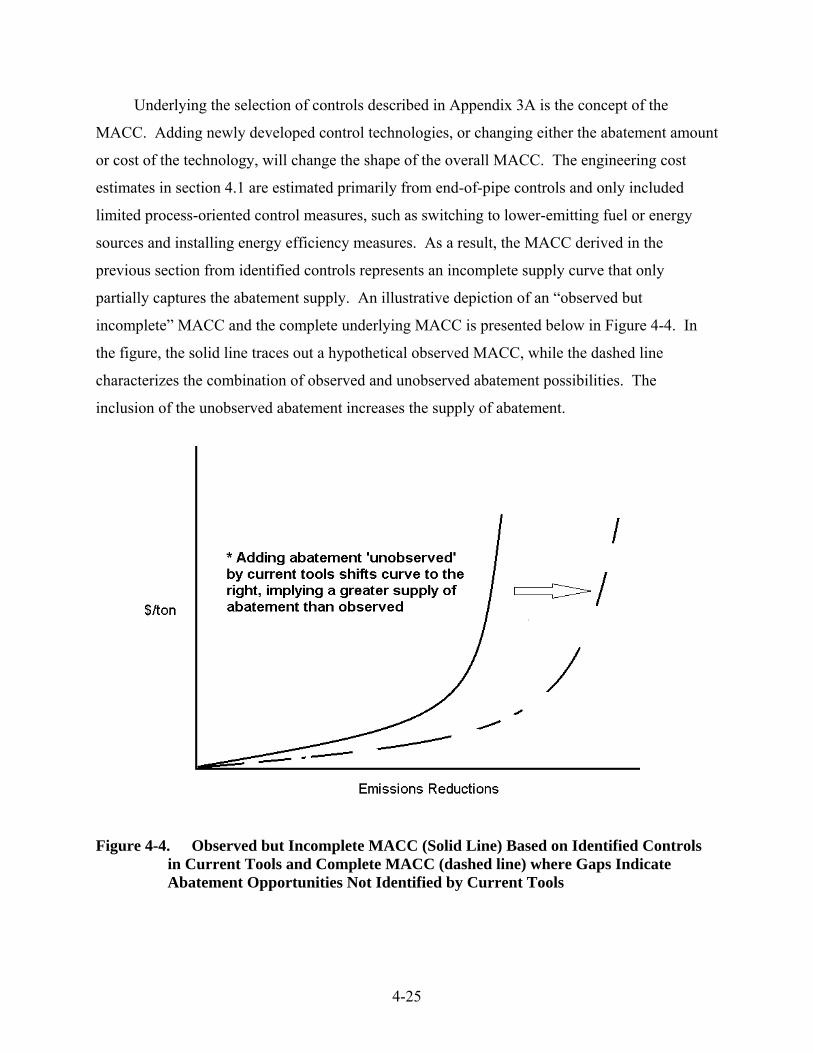
4-25
Underlying the selection of controls described in Appendix 3A is the concept of the
MACC. Adding newly developed control technologies, or changing either the abatement amount
or cost of the technology, will change the shape of the overall MACC. The engineering cost
estimates in section 4.1 are estimated primarily from end-of-pipe controls and only included
limited process-oriented control measures, such as switching to lower-emitting fuel or energy
sources and installing energy efficiency measures. As a result, the MACC derived in the
previous section from identified controls represents an incomplete supply curve that only
partially captures the abatement supply. An illustrative depiction of an “observed but
incomplete” MACC and the complete underlying MACC is presented below in Figure 4-4. In
the figure, the solid line traces out a hypothetical observed MACC, while the dashed line
characterizes the combination of observed and unobserved abatement possibilities. The
inclusion of the unobserved abatement increases the supply of abatement.
Figure 4-4. Observed but Incomplete MACC (Solid Line) Based on Identified Controls in Current Tools and Complete MACC (dashed line) where Gaps Indicate Abatement Opportunities Not Identified by Current Tools

4-26
Because of the incomplete characterization of the full range of NOx abatement
possibilities, it is important to understand the composition of the cost information EPA has
available and uses to construct the partial MACC. The nature of available information on the
cost of NOx abatement measures is somewhat complex. EPA’s control strategy tools undergo
continuous improvement, and as the need for additional abatement opportunities increases,
additional evaluation of uncontrolled emissions takes place. During these evaluations, additional
abatement opportunities from applying identified controls typically are found. These abatement
opportunities or additional controls are added to the CoST database and will be available for
future analyses. In addition, in some cases we may have specific knowledge of potential
additional control measures due to an impending regulation (e.g., Tier 3), but until a regulation is
finalized those identified controls are not included in any concurrent analyses.
It is also important to understand that EPA’s control strategy tools largely focus on end-of-
pipe controls and a limited set of emissions inventory sectors, whereas opportunities for
emissions reductions through non-end-of-pipe controls or measures exist. For example, we
reviewed the existing control strategies indicated in the SIP for the Dallas-Fort Worth area for
the 1997 ozone NAAQS, and we compared the strategies and measures in that SIP to the
measures the EPA analyzed in the 1997 ozone NAAQS regulatory impact analysis. The EPA
analyzed several industrial source categories and measures that were reflected in the 1997
Dallas-Fort Worth SIP, including existing control measures for stationary sources such as cement
kilns, industrial boilers, iron and steel mills, as well as enhanced inspection and maintenance
programs for mobile sources.70 The Dallas-Fort Worth SIP recognized the need for additional
control strategies and measures to achieve further emissions reductions – strategies and measures
that were not reflected in EPA’s 1997 control strategy analysis. These additional control
measures included transportation control measures, additional voluntary mobile emission
reduction programs, and energy efficiency/renewable energy measures. Table 4-4 below
includes examples of each of these types of programs or measures.
70 The Dallas-Fort Worth SIP also reflected the following existing voluntary mobile emission reduction programs: alternative fuel vehicle program; employee trip reduction program; and vehicle retirement program. Information on the Dallas-Fort Worth SIP is available at http://www.nctcog.org/trans/air/sip/future/lists.asp.

4-27
Table 4-4. Control Measures in Dallas-Fort Worth SIP Not Reflected in the 1997 Ozone
NAAQS RIA
Transportation Control Measures Bicycle/Pedestrian Projects Grade Separation Projects HOV/Managed Lane Projects Intersection Improvement Projects Park and Ride Projects Rail Transit Projects Vanpool Projects Voluntary Mobile Source Emission Reduction Programs
Clean Vehicle Program Employee Trip Reduction Locally Enforced Idling Restriction Diesel Freight Idling Reduction Program Other State and Local Programs: Energy Efficiency/Renewable Energy
Residential Building Code Commercial Building Code Federal Facilities Projects Political Subdivision Projects71 Electric Utility-Sponsored Programs72 Wind Power Projects Additional Measures Clean School Bus Program Texas Low Emission Diesel Stationary Diesel and Dual-Fired Engine
Control Measures
Further, Table 4-5 includes specific non-end-of-pipe control measures from approved SIPs
in Texas and Louisiana, including measures from the Dallas-Fort Worth SIP (i.e., energy
efficiency measures). The approved, non-end-of-pipe control measures include local
transportation measures, local building energy efficiency requirements, and mobile source sector
measures. In addition, Table 4-6 includes examples of approved non-end-of-pipe control
measures in California. California is also currently developing the following additional
measures:
71 These projects are typically building system retrofits, non-building lighting projects, and other mechanical and electrical systems retrofits, such as municipal water and waste water treatment systems. 72 These programs include air conditioner replacements, ventilation duct tightening, and commercial and industrial equipment replacement.
4-28
Encouraging Use of Warm Mix Asphalt over Hot Mix Asphalt - European and
American companies have developed several techniques, collectively known as
warm-mix asphalt (WMA), to increase the workability of asphalt by lowering the
viscosity at temperatures as much as 100°F below that of hot-mix asphalt (HMA).
WMA was introduced in Europe in 1997 and in the United States in 2002. WMA
has shown potential for reducing emissions associated with the production of
asphalt for paving projects when compared to HMA. Lower temperatures required
for production, storage, transport, and application translates to lower fuel
consumption, which in turn reduces the criteria air pollutant emissions associated
with combustion.73
Replacement of gas-powered leaf blowers and mowers – The South Coast Air
Quality Management District has a program that subsidizes the replacement of
existing two-stroke backpack blowers currently used by commercial
landscapers/gardeners with new four-stroke backpack blowers that have
significantly reduced emissions and noise levels.74
All of these additional and non-end-of-pipe measures and associated emissions reductions are not
reflected in EPA’s control strategy tools and represent additional abatement opportunities not
accurately captured in this analysis.
73 For additional information see http://www.fhwa.dot.gov/everydaycounts/technology/asphalt/intro.cfm ; slide 31 aci-na.org/static/entransit/sunday_warmmix_logan.pdf. FHWA estimates that warm mix asphalt uses 20 percent less energy than hot mix asphalt. Also see http://www.fhwa.dot.gov/everydaycounts/technology/asphalt/intro.cfm. Airports Council International reports 10-55 percent lower energy consumption and 20-55 percent reduction in emissions. (See http://aci-na.org/static/entransit/sunday_warmmix_logan.pdf, Slide 31)). 74 Typically, ten exchange events are set up across the District, and for the convenience of the participants, the exchange events take place during consecutive weekdays. At the event site, the old leaf blowers will be tested for operation and then drained of all fluids in a responsible manner and collected for scrapping. The vendor will haul the traded-in blowers to a scrapping yard where they are crushed and recycled. The vendor will also provide training for the proper use of the equipment at each of the exchange sites. (http://www.aqmd.gov/docs/default-source/Lawn-Equipment/leafblower-brochure.pdf?sfvrsn=9)

4-29
Table 4-5. Non-End-of-Pipe Control Measures from SIPs
Measure Projected Emissions Reductions
(tons per day)
Area Citation
Energy Efficiency75 0.04 (NOx) Shreveport/Bossier City Area, Louisiana
70 FR 48880 August 22, 2005
Energy Efficiency76 0.72 (NOx) Dallas/Fort Worth (DFW), Texas
73 FR 47835 August 15, 2008
Transportation Emission Reduction Measures77
0.72 (NOx) 0.83 (VOC)
Austin - Early Action Compact Area, Texas
70 FR 48640 August 19, 2005
Voluntary Mobile Emission Reduction Program (VMEP)
2.63 (NOx) 0.61 (VOC)
DFW area 74 FR 1906 January 14, 2009
Texas Emission Reduction Plan (TERP)78, 79
14.2 (NOx) DFW area 74 FR 1906 January 14, 2009
Texas Low Emission Diesel (TxLED)80
Up to 6 (NOx); on-going and varies annually
East and Central Texas (includes DFW area)
79 FR 67068 November 12, 2014
75 The measures involved installing energy conservation equipment in 33 city buildings. Measures included upgrades to the lighting, mechanical and control systems, water conservation upgrades, and other miscellaneous activities. This was an Early Action Compact (EAC) area SIP. 76 The NOx emissions reductions in the DFW area were due to energy efficiency measures in new construction for single and multi-family residences. This measure was initially submitted within a SIP to provide emissions reductions of 5 percent in the DFW area; actual reductions fell short of the 5 percent goal, but this measure was eventually approved with other measures that, by providing additional emissions reductions, improved air quality in the area. 77 The transportation projects were to reduce vehicle use, improve traffic flow, and/or reduce congested conditions throughout the Austin EAC area (this was an EAC SIP). The Austin EAC area included Bastrop, Caldwell, Hays, Travis, and Williamson counties and the cities of Austin, Bastrop, Elgin, Lockhart, Luling, Round Rock, and San Marcos. 78 TERP is a discretionary economic incentive program: economic incentives to reduce emissions. The approved TERP is a grant program, unique to Texas, that provides funds through the Texas Commission on Environmental Quality in a variety of categories, including emissions reduction incentive grants, rebate grants (including grants for small businesses), and heavy and light duty motor vehicle purchase or lease programs, all with the goal of improving air quality in Texas. Examples of TERP programs include assisting small businesses in purchasing lower-emission diesel vehicles, helping school districts to reduce emissions from school buses, and providing funds to support research and development of pollution-reducing technology. TERP is available to all public and private fleet operators that operate qualifying equipment in any of the ozone nonattainment counties within Texas. TERP was also approved into the Texas EAC SIPs, providing at least 2 tons per day in NOx reductions in each of three areas (Austin, Tyler/Longview, and San Antonio). 79 The State of Texas reports on the TERP every other year and the emissions reductions cited here were based on an estimated $6,000 per ton. 80 The TxLED fuel program was initially approved by EPA on November 14, 2001 (66 FR 57196) and has undergone subsequent revisions, the latest on May 5, 2013 (78 FR 26255). TxLED fuel is required for use by on-highway vehicles and non-road equipment (including marine vessels) in 110 counties in eastern and central Texas. Use of this boutique fuel reduces NOx emissions.

4-30
Table 4-6. Non-End-of-Pipe Measures in California
Program or Standard Area Citation Estimated Emissions Reductions
Carl Moyer Memorial Air Quality Standards Attainment Program (selected project types)*
San Joaquin Valley, California
79 FR 29327 (May 22, 2014)
3.78 tpd NOx credited in San Joaquin Valley
Proposition 1B: Goods Movement Emission Reduction Program (selected project types)*
San Joaquin Valley, California
79 FR 29327 (May 22, 2014)
1.23 tpd NOx credited in San Joaquin Valley
California Reformulated Gasoline (RFG) Program
California (statewide)
60 FR 43379 (August 21, 1995), revised 75 FR 26653 (May 12, 2010)
California Diesel Fuel Program California (statewide)
60 FR 43379 (August 21, 1995), revised 75 FR 26653 (May 12, 2010)
Regional Clean Air Incentives Market (RECLAIM)
South Coast, California
63 FR 32621 (June 15, 1998), revised 71 FR 51120 (August 29, 2006) and 76 FR 50128 (August 12, 2011)
* Program not approved into SIP but relied upon for emission reduction credit through state commitment.
Lack of information about the MAC for emissions reductions not characterized in CoST is
not an indication that controlling those tons is necessarily more difficult than controlling NOx
from other sources that are in the database, or that the MAC for those tons is necessarily higher
than all of the costs of controls already in the database. Some sectors are controlled at a higher
rate than others, and in those cases, getting additional NOx reductions may indeed require higher
cost controls. However, other sectors may not be as well-controlled, and lower cost controls may
be available.
4.2.4 Comparing Baseline Emissions and Controls across Ozone NAAQS RIAs from 1997 to 2014
Many factors affect the future year baseline emissions used in a NAAQS analysis,
including the future year being analyzed, the projected air quality in that year, the emissions
inventories used, emissions projections methodologies, and any federal and/or state regulatory
programs or measures that are reflected in the emissions projections. The EPA believes that
while these factors and changes are difficult to track individually, additional federal and/or state

4-31
regulatory programs promulgated and the new data on available control technologies or measures
can, over time, result in emissions reductions and control measures being reclassified from
unidentified to identified measures. Each ozone NAAQS analysis since 1997 has required at
least some emissions reductions from controls that were considered unidentified at the time of
analysis, but evidence indicates that over time new information becomes available that changes
the characterization of these emissions reductions from unidentified measures to identified
measures. For example, in the 1997 ozone NAAQS RIA, NOx emissions reductions that were
expected to result from the at that time upcoming mobile source Tier 2 standards were not
characterized as resulting from identified controls, even though the RIA acknowledged the
potential for these standards to provide substantial cost-effective controls and emissions
reductions. As a result, in 1997 these cost-effective emissions reductions were considered to be
from unidentified controls, while in retrospect they were actually from identified controls.
Likewise, the 2008 ozone NAAQS RIA did not include controls on EGUs that would later be
predicted to result from the Mercury and Air Toxics Standards or the Clean Power Plan. As a
result, in 2008 emissions reductions needed from unidentified controls were estimated to be
higher in some regions of the U.S. than those estimated in this RIA. In general, during the time
between the promulgation of a NAAQS and the required date of attainment, additional rules may
be developed and additional analyses performed that shed light on how emissions reductions that
were once thought to be unavailable from identified control measures are obtained through
tangible means. Improvements over time, both in information and engineering, lead to an
increase in identified controls and as a result emission reductions obtained only through
unidentified controls in one analysis may be realized through identified controls in subsequent
analyses.
4.2.5 Possible Alternative Approaches to Estimate Costs of Unidentified Control Measures
In determining how to estimate the costs of achieving the emission reductions needed
from unidentified control measures (see Section 4.3), we examined what information could be
gleaned from existing regional NOx offset prices. In ozone nonattainment areas, new sources
interested in locating in that area and existing sources interested in expanding are required to
offset any emissions increases. If those emissions increases are NOx emissions, the source
typically purchases NOx emission reduction credits (ERCs), or offsets, from within that

4-32
particular nonattainment area. Within nonattainment areas, offset prices fluctuate because of
changes in the available supply of offsets and changes in demand for offsets. Offset supply
increases when facilities shut down or when they make process or other changes that reduce
emissions permanently. Offset demand depends on the industrial base in a given area and
fluctuates with changes in economic growth. For example, in the San Joaquin Valley, in recent
years offset prices have increased because of increased oil and gas industry development.
We identified historical NOx offset prices in several nonattainment areas, including the
San Joaquin Valley and the South Coast in California, Houston, TX, and New York region. For
the San Joaquin Valley Air Pollution Control District, we collected information on NOx offset
prices using the California Air Resources Board’s Emission Reduction Offset Transaction Cost
Summary Reports for 2002 through 2013.81 For the South Coast Air Quality Management
District, we collected information on prices for perpetual NOx RECLAIM Trading Credit (RTC)
for 2003 through 2012 from the Listing of Trade Registrations.82 Lastly, we collected
information on NOx offset prices in the Houston-Galveston nonattainment area for 2010 through
2013 from the Trade Report83 and the New York-New Jersey-Connecticut nonattainment area
from 2000 through 2013 from industry representatives.
Table 4-7 presents the price data we were able to collect for these four regions, adjusted
to 2011 dollars using the Gross Domestic Product Implicit Price Deflator. The offset prices in
this table are denominated in units of perpetual tons, or tons per year, and represent a one-time
payment or cost, not an annual payment or cost. The prices constitute average of the trades in
the regions for the year given. The data series for the California regions are more complete than
those for Houston and the New York region.
81 http://www.arb.ca.gov/nsr/erco/erco.htm 82 http://www.aqmd.gov/home/programs/business/about-reclaim/reclaim-trading-credits 83 http://www.tceq.state.tx.us/airquality/banking/mass_ect_prog.html

4-33
Table 4-7. Average NOx Offset Prices for Four Areas (2011$, perpetual tpy) a
NOx Offset Prices ($/ perpetual tpy)
San Joaquin
Valley California South
Coast Houston TX New York Region
2000 N/A N/A N/A 25,000
2001 N/A N/A N/A 12,000
2002 36,000 N/A N/A 12,000
2003 28,000 N/A N/A 12,000
2004 25,000 12,000 N/A 12,000
2005 25,000 31,000 N/A 11,000
2006 21,000 163,000 N/A 11,000
2007 21,000 206,000 N/A N/A
2008 48,000 210,000 N/A N/A
2009 58,000 128,000 N/A N/A
2010 62,000 98,000 36,000 N/A
2011 64,000 56,000 N/A N/A
2012 47,000 47,000 N/A N/A
2013 42,000 N/A 97,000 4,000
Average 40,000 106,000 66,000 12,000
Maximum 64,000 210,000 97,000 25,000 a All values are rounded to two significant figures.
To more directly compare offset prices to potential annual costs for unidentified
emissions controls, we annualized the perpetual, tons per year prices using the same engineering
cost equations as used in the main analysis to estimate annualized control cost. We converted
the offset cost to an annual cost by using the capital recovery factor (CRF) discussed in Section
4.1.1. In a capital cost context, the CRF incorporates the interest rate and lifetime of the
purchased capital. In this instance, although the offsets are perpetual in nature, we assumed a
lifetime of 20 years in order to make the cost basis more comparable to the control cost
estimates. Also, we used 7 percent for the interest rate. Table 4-8 presents the average and
maximum annualized NOx offset prices in 2011 dollars.

4-34
Table 4-8. Annualized NOx Offset Prices for Four Areas (2011$, tons)a
Annualized NOx Offset Prices ($/ton)
San Joaquin
Valley California South
Coast Houston TX New York Region
Average $ 4,000 $ 10,000 $ 6,000 $ 1,000
Maximum $ 6,000 $ 20,000 $ 9,000 $ 2,000 a All values are rounded to two significant figures.
From an economic perspective, these offset prices may represent the shadow value of a
ton of emissions since the purchaser of the offset chose to purchase the offset rather than curtail
their business activities or purchase some other pollution control technology. It is possible that
these offset prices could serve as reasonable proxies for the costs associated with emissions
reductions from unidentified measures or controls. The cost information informing the identified
control strategy traces out an incomplete marginal abatement cost curve in that, as discussed in
Chapter 3, the controls used in the identified control analysis are primarily end-of-pipe
technologies. The identified control estimates for NOx do not account for other forms of
abatement, e.g., switching to lower emitting fuels or increasing energy efficiency. The estimates
also do not account for institutional or market arrangements that allow firms to buy or sell
emissions offsets in nonattainment regions with emissions constraints. These voluntary
exchanges may enable abatement at lower costs than may otherwise be available. The benefit of
these market transaction data is that the prices are revealed by the interaction of offset supply and
demand in regions with differentiated characteristics and emissions and air quality profiles. In
each region, offset supply is a function of the emissions inventory and offset demand is a
function of economic growth, and neither offset supply nor demand is infinite.
An alternative proxy for estimating the costs of unidentified control measures is using the
current annualized section 185 fee rate. The section 185 fee program requirement applies to any
ozone nonattainment area that is classified as Severe or Extreme under the NAAQS. If a Severe
or Extreme nonattainment area fails to attain the ozone NAAQS by the required date, section 185
of the Clean Air Act requires each major stationary source of VOC and NOx located in such area
to pay a fee to the state for each calendar year following the attainment year for emissions above

4-35
a baseline amount and until the area reaches attainment.84,85 The fee was set in the 1990 Clean
Air Act at $5,000 per ton of VOC and NOx emissions above the baseline amount and is adjusted
annually for inflation based on the Consumer Price Index. The 2013 annualized section 185 fee
rate was $9,398.67 per ton. Examples of states or areas that have adopted section 185 fee
programs include: (a) Texas for the Houston-Galveston nonattainment area, which adopted its
fee program in May 2013,86 and (b) the South Coast Air Quality Management District, which
amended Rule 317 that governs its fee program in February 2011.
4.2.6 Conclusion
The preceding sections have discussed the ways in which various factors might affect the
observed marginal abatement costs and the resulting total abatement costs estimated in this RIA.
Based on past experience with Clean Air Act implementation, the EPA believes that it is
reasonable to anticipate that the marginal cost of emissions reductions will decline over time due
to technological improvements and more widespread adoption of previously considered niche
control technologies, as well as the development of innovative strategies.87 In addition, while we
examined other approaches to estimate the costs of unidentified measures, we concluded that
these approaches could potentially undervalue the costs of unidentified controls. As the EPA
continuously improves its data and tools, we expect to better characterize the currently
unobserved pieces of the MACC.
4.3 Compliance Cost Estimates for Unidentified Emissions Controls
This section presents the methodology and results for the costs of emissions reductions
from unidentified control measures needed to demonstrate full attainment of the revised and
alternative standards analyzed. We refer to the costs of emissions reductions from unidentified
84 For additional information on developing fee programs required by Clean Air Act Section 185, see the January 5, 2010 memorandum from the EPA’s Office of Air Quality Planning and Standards, available at: http://www.epa.gov/ttn/naaqs/aqmguide/collection/cp2/bakup/20100105_page_section_185_fee_programs.pdf. 85 In 1990, the Clean Air Act set the fee at $5,000/ton of VOC and NOx emitted by the source during the calendar year in excess of 80 percent of the baseline amount. A source’s baseline amount is the lower of the amount of actual or allowable emissions under the permit for the source during the attainment year. 86 Additional information on Texas’s actions is available at http://www.tceq.texas.gov/airquality/point-source-ei/sipsection185.html 87 See Chapter 3, Section 3.4 for additional discussion of uncertainties associated with predicting technological
advancements that may occur between now and 2025.

4-36
controls as unidentified control costs.88 As discussed in Chapter 3, the application of the
identified control strategies was not sufficient in reaching full, nationwide attainment of the
revised standard of 70 ppb and the alternative standard of 65 ppb analyzed. Therefore, the
engineering costs detailed in Section 4.1 represent only the costs of partial attainment.
4.3.1 Methods
On the issue of estimating the costs of unidentified control measures, in 2007 the EPA’s
Science Advisory Board offered the following advice:
The Project Team has been unable to identify measures that yield sufficient emission reductions to comply with the National Ambient Air Quality Standards (NAAQS) and relies on unidentified pollution control measures to make up the difference. Emission reductions attributed to unidentified measures appear to account for a large share of emission reductions required for a few large metropolitan areas but a relatively small share of emission reductions in other locations and nationwide. The Council agrees with the Project Team that there is little credibility and hence limited value to assigning costs to these unidentified measures. It suggests taking great care in reporting cost estimates in cases where unidentified measures account for a significant share of emission reductions. At a minimum, the components of the total cost associated with identified and unidentified measures should be clearly distinguished. In some cases, it may be preferable to not quantify the costs of unidentified measures and to simply report the quantity and share of emissions reductions attributed to these measures. When assigning costs to unidentified measures, the Council suggests that a simple, transparent method that is sensitive to the degree of uncertainty about these costs is best. Of the three approaches outlined, assuming a fixed cost/ton appears to be the simplest and most straightforward. Uncertainty might be represented using alternative fixed costs per ton of emissions avoided.89
While we have considered alternative methodologies to predict future abatement supply
curves, we are currently unable to quantitatively predict future shifts in the abatement supply
curve with sufficient confidence to use in this RIA. For most NAAQS RIAs prepared during the
past five years, EPA estimated the costs for unidentified controls using a pair of methodologies:
a “fixed cost” approach, following the SAB advice, and a “hybrid” approach that has not yet
88 In previous analyses, these costs were referred to as extrapolated costs. 89 U.S. Environmental Protection Agency. June 2007. Advisory Council on Clean Air Compliance Analysis (COUNCIL), Council Advisory on OAR’s Direct Cost Report and Uncertainty Analysis Plan. Washington, DC.

4-37
been reviewed by the SAB.90 We refer to the fixed cost approach as the “average cost” approach
here. The average cost approach uses an assumed national average cost per ton for unidentified
controls needed for attainment, as well as two alternative assumed values employed for
sensitivity analysis (Appendix 4A). The range of estimates reflects different assumptions about
the cost of additional emissions reductions beyond those in the identified control strategies.
While we use a constant, average cost per ton to estimate the costs of the emissions reductions
beyond identified controls, this does not imply that the MACC is not upward sloping. The
constant, average cost per ton is designed to capture total costs associated with the abatement of
the emissions reductions from unidentified controls – because of the incomplete information
available to inform the characterization of the MACC, a portion of those total costs is likely at a
value below the average cost per ton and a portion is likely at a value above the average cost per
ton.
The alternative values used in the sensitivity analysis implicitly reflect different
assumptions about the amount of technological progress and innovation in emissions reduction
strategies that may be expected in the future. The average cost approach reflects a view that
because we have incomplete data on existing control technologies, and because no cost data
exists for unidentified future technologies, measures, or strategies, it is unclear whether
approaches using hypothetical cost curves will be more accurate or less accurate in forecasting
total national costs of unidentified controls than an average cost approach that uses a range of
national cost-per-ton values.
The hybrid approach assumed increasing marginal costs of control along an upward-
sloping marginal cost curve. The hybrid approach assumed the rate of increase in the marginal
costs of abatement is proportional to the weighted ratio of the amount of abatement using
identified controls to the remaining needed abatement using unidentified controls.91 Under this
approach, the relative costs of unidentified controls in different geographic areas reflected the
90 The three approaches mentioned above, outlined for SAB review, for assigning costs to unidentified measures included: (1) the fixed cost approach that assigns all unidentified measures a fixed cost per ton; (2) an approach based on an upward sloping cost curve that uses information from the identified control measure analysis on an area-specific basis; and (3) an approach that adjusts the upward sloping cost curve projections using information about cost changes over time to reflect factors such as learning by doing and induced innovation. 91 See, for example, Section 7.2 and Appendix 7.A.2 in the December 2012 RIA for the final PM2.5 NAAQS, available at http://www.epa.gov/ttn/ecas/regdata/RIAs/finalria.pdf.

4-38
expectation that average per-ton control costs are likely to be higher in areas needing a higher
ratio of emissions reductions from unidentified and identified controls. However, the weight,
which reflected the anticipated degree of difficulty of achieving needed emissions reductions,
and the ratios that informed the slope of the marginal abatement cost curve in previous NAAQS
analyses were strong assumptions that have not been empirically tested.
When used to estimate costs for end-of-pipe technologies, the hybrid approach assumed
all emissions reductions come from the highest cost margin of the abatement supply curve
which, as explained in the previous section, is unlikely for much of the unobserved abatement
capacity in the present and future. For example, EPA’s control strategy tools largely focus on a
limited set of emissions inventory sectors, whereas abatement opportunities exist in other sectors.
For areas needing significant additional emission reductions, much pollution abatement is
likely needed from sectors that historically have not been intensively regulated and thus have
relatively more available potential emissions reductions. If national standards become more
stringent, new regions or firms will be added to the regulated domain. These new entrants, with
their relatively untapped abatement supply, will contribute to an outward shift in abatement
supply. The newly regulated regions and firms will also face new incentives for technical
change and innovation that may lower costs over the long run by developing new, more efficient
compliance strategies. Because the point of departure for the hybrid approach cost curve is
based on our current database, which includes only existing controls, it will systematically
overstate future costs if any cost-reducing technological change occurs.
As noted in previous NAAQS analyses, the EPA continues to explore other sources of
information to inform the estimates of costs associated with unidentified controls. For this RIA
we examined the full set of identified controls, examined evidence that suggests that over time
new information and data emerges that shifts emissions reductions from the unidentified to the
identified category, as well as explored whether NOx offset prices can serve as reasonable
proxies for the costs of emissions reductions not identified by current tools.
Based upon deliberations informing this discussion, the EPA Science Advisory Board
Council Advisory’s advice, and the requirements of E.O. 12866 and OMB circular A-4, which
provide guidance on the estimation of benefits and costs of regulations, in this RIA, we follow

4-39
the Council recommendations by using an average cost per ton as a central estimate and conduct
sensitivity analysis using alternative average costs to explore how sensitive total costs are to
these assumptions. While the average cost approach has limitations, we agree with the Council
that the approach is both transparent and strikes a balance between the likelihood that some
unidentified abatement would arise at lower segments of the identified cost curve while other
sources of abatement may come at the higher cost margin.
As discussed in Section 4.1.1, we apply a constant, average cost per ton of $15,000/ton to
capture total costs associated with the NOx emissions reductions achieved through unidentified
controls. To explore how sensitive total costs are to this assumption, we also use alternative
assumptions of the average cost. Specifically, we conduct a first sensitivity analysis using an
assumed cost of $10,000 per ton and a second sensitivity analysis using an assumed $20,000 per
ton. This range is inclusive of the annualized NOx offset prices observed in recent years in the
areas likely to need unidentified controls to achieve the standard (Table 4-8), and if anything,
suggests the central estimate of $15,000/ton is conservative. In the RIA for the ozone NAAQS
proposal, EPA requested comments on the methods presented to estimate emissions reductions
needed beyond identified controls, including the parameter estimate of $15,000/ton. We
received comments that the parameter estimate of $15,000/ton (2011$) was low and should be
adjusted to reflect inflation. The EPA has elected to retain the parameter estimate of $15,000/ton
(2011$) because inflation was low between 2006 and 2011. While the Agency received
comments on its methods, alternative approaches have not been subjected to peer review and
therefore could not be applied here.
Because cost changes due to technological change will be available on a national-level, it
makes sense to use national-level average cost per ton in the primary analysis. However, as
indicated by the variation in NOx offset prices across regions shown in Table 4-7, regional
factors may play a significant role in the estimation of control costs. In the RIA for proposal,
EPA stated it may review alternative methodologies and sources of regional information that
could result in the average cost methodology being applied more regionally. The EPA reviewed
data on end-of-pipe controls more closely and worked on identifying information from measures
used in SIPs. The data in CoST on end-of-pipe technologies was not sufficiently robust to
generate regional data, and obtaining detailed cost information from state or local SIPs requires a

4-40
longer-term effort. Despite the regional variation in offset prices, we believe the $15,000/ton
estimate represents a conservative value because it is higher than the majority of the annualized
offset values in Table 4-8, and because the values we use in the sensitivity analyses include the
highest annualized offset value.
4.3.2 Compliance Cost Estimates from Unidentified Controls
Table 4-9 presents the control cost estimates for unidentified controls for the East and
West in 2025, except for California for the final standard of 70 ppb and an alternative standard of
65 ppb using an assumed average cost of $15,000/ton, as well as values of $10,000/ton and
$20,000/ton. Appendix 4A includes potential alternative methods for either assigning an average
cost value or for determining values used in sensitivity analyses.
Table 4-9. Unidentified Control Costs in 2025 by Alternative Standard for 2025 – U.S., except California (7 percent discount rate, millions of 2011$)
Alternative Level Geographic Area Unidentified Control Cost
$10,000/ton $15,000/ton $20,000/ton
70 ppb
East 470 700 930 West - - - Total 470 700 930
65 ppb
East 8,200 12,000 16,500 West 400 610 810 Total 8,600 13,000 17,000
a All values are rounded to two significant figures.
Table 4-10 presents the unidentified control cost estimates for post-2025 for California
for the final standard of 70 ppb and an alternative standard level of 65 ppb using an assumed
average cost of $15,000/ton, as well as values of $10,000/ton and $20,000/ton.

4-41
Table 4-10. Unidentified Control Costs in 2025 by Alternative Standard for Post-2025 –California (7 percent discount rate, millions of 2011$)
Alternative Level Geographic Area Unidentified Control Cost
$10,000/ton $15,000/ton $20,000/ton
70 ppb California 510 800 1,020 65 ppb California 1,000 1,500 2,000
a All values are rounded to two significant figures.
4.4 Total Compliance Cost Estimates
As discussed throughout this RIA, we present the primary costs and benefits estimates for
2025. We assume that potential nonattainment areas everywhere in the U.S., excluding
California, will be designated such that they are required to reach attainment by 2025, and we
developed our projected baselines for emissions, air quality, and populations for 2025. Please
see Chapter 1, Section 1.3.2 for additional detailed discussion on potential nonattainment
designations and timing.
Tables 4-11 and 4-12 present summaries of the total national annual costs (identified and
unidentified) of attaining the revised standard of 70 ppb and alternative standard of 65 ppb –
Table 4-11 presents the total national annual costs by alternative standard for 2025 for all of the
U.S., except California and Table 4-12 presents the total national annual costs by alternative
standard for post-2025 for California. As discussed in Section 4.1.2, because we do not have a
full set of costs at the 3 percent discount rate or the 7 percent discount rate and because we
believe the majority of the identified control costs is calculated at a 7 percent discount rate,
Tables 4-11 and 4-12 present engineering cost estimates based on a 7 percent discount rate.
Table 4-11. Summary of Total Control Costs (Identified and Unidentified) by Alternative Level for 2025 - U.S., except California (millions of 2011$, 7% Discount Rate)a
Alternative Level Geographic Area
Total Control Costs (Identified and Unidentified)
70 ppb
East 1,400 West <5 Total $1,400
65 ppb
East 15,000 West 750 Total $16,000
a All values are rounded to two significant figures. Unidentified control costs are based on the average cost approach.
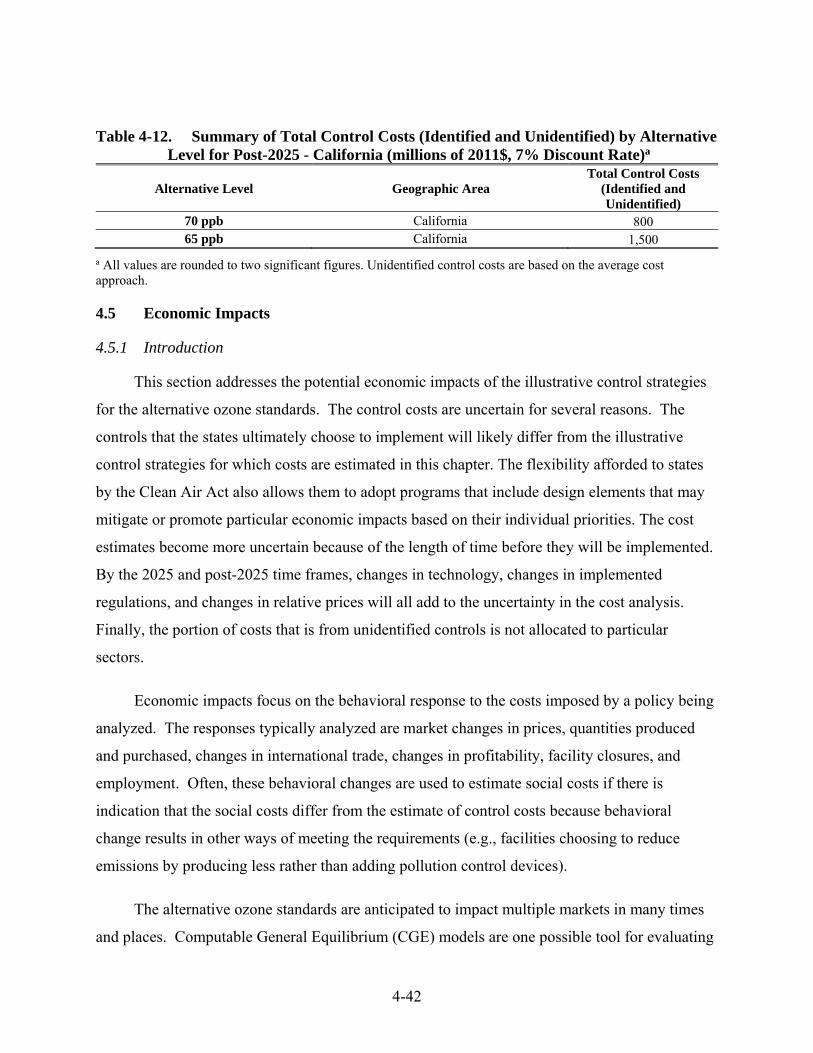
4-42
Table 4-12. Summary of Total Control Costs (Identified and Unidentified) by Alternative Level for Post-2025 - California (millions of 2011$, 7% Discount Rate)a
Alternative Level Geographic Area Total Control Costs
(Identified and Unidentified)
70 ppb California 800 65 ppb California 1,500
a All values are rounded to two significant figures. Unidentified control costs are based on the average cost approach.
4.5 Economic Impacts
4.5.1 Introduction
This section addresses the potential economic impacts of the illustrative control strategies
for the alternative ozone standards. The control costs are uncertain for several reasons. The
controls that the states ultimately choose to implement will likely differ from the illustrative
control strategies for which costs are estimated in this chapter. The flexibility afforded to states
by the Clean Air Act also allows them to adopt programs that include design elements that may
mitigate or promote particular economic impacts based on their individual priorities. The cost
estimates become more uncertain because of the length of time before they will be implemented.
By the 2025 and post-2025 time frames, changes in technology, changes in implemented
regulations, and changes in relative prices will all add to the uncertainty in the cost analysis.
Finally, the portion of costs that is from unidentified controls is not allocated to particular
sectors.
Economic impacts focus on the behavioral response to the costs imposed by a policy being
analyzed. The responses typically analyzed are market changes in prices, quantities produced
and purchased, changes in international trade, changes in profitability, facility closures, and
employment. Often, these behavioral changes are used to estimate social costs if there is
indication that the social costs differ from the estimate of control costs because behavioral
change results in other ways of meeting the requirements (e.g., facilities choosing to reduce
emissions by producing less rather than adding pollution control devices).
The alternative ozone standards are anticipated to impact multiple markets in many times
and places. Computable General Equilibrium (CGE) models are one possible tool for evaluating

4-43
the impacts of a regulation on the broader economy because this class of models explicitly
captures interactions between markets across the entire economy. To support the Final Ozone
NAAQS of March 2008 (Final Ozone NAAQS Regulatory Impact Analysis), among other
rulemakings, the EPA used the Economic Model for Policy Analysis (EMPAX) to estimate the
market impacts of the portion of the cost that was associated with the application of identified
controls (excluding the unidentified control costs). EMPAX is a dynamic computable general
equilibrium (CGE) model that forecasts a new equilibrium for the entire economy after a policy
intervention. While a CGE model captures the effects of behavioral responses on the part of
consumers or other producers to changes in price that are missed by an engineering estimate of
compliance costs, most CGE models do not model the environmental externality - or the benefits
that accrue to society from mitigating it. When benefits from a regulation are expected to be
substantial, social cost cannot be interpreted as a complete characterization of economic welfare.
To the extent that the benefits affect behavioral responses in markets, the social cost measure
may also be potentially biased.
EPA included specific types of health benefits in a CGE model for the prospective
analysis, The Benefits and Costs of the Clean Air Act from 1990 to 2020 (EPA 2011), and
demonstrated the importance of their inclusion when evaluating the economic welfare effects of
policy. However, while the external Council on Clean Air Compliance Analysis (Council) peer
review of this EPA report (Hammitt 2010) stated that inclusion of benefits in an economy-wide
model, specifically adapted for use in that study, “represent[ed] a significant step forward in
benefit-cost analysis”, serious technical challenges remain when attempting to evaluate the
benefits and costs of potential regulatory actions using economy-wide models.
To begin to address these technical challenges, the EPA has established a new Science
Advisory Board (SAB) panel on economy-wide modeling to consider the technical merits and
challenges of using CGE and other economy-wide modeling tools to evaluate costs, benefits, and
economic impacts of air regulations. The EPA will use the recommendations and advice of this
SAB panel as an input into its process for improving benefit-cost and economic impact analyses
that are used to inform decision-making at the Agency. The panel will also be asked to identify
potential paths forward for improvements that could address the challenges posed when
economy-wide models are used to evaluate the effects of regulations.
4-44
The advice from the SAB panel formed specifically to address the subject of economy-
wide modeling was not available in time for this analysis. Given the ongoing SAB panel on
economy-wide modeling, the uncertain nature of costs, the Council’s advice regarding the
importance of including benefit-side effects, and the lack of available multi-year air quality
projections needed to include these benefit-side effects, EPA has not conducted CGE modeling
for this analysis. Instead, this section proceeds with a qualitative discussion of market impacts.
4.5.2 Summary of Market Impacts
Consider an added cost to produce a good associated with the pollution control required to
reach the alternative ozone standards. Such a good is either one developed for the consumer
(called a consumption good), or one used in the production of other goods for consumption
(called an intermediate good). Some goods are both consumption and intermediate goods. First,
consider the direct impact on the market facing the increased cost. In this case for the market
facing the increased cost, the price will go up and the amount sold will go down. The magnitude
of these shifts depends on a number of factors. The greater the unit cost increase relative to the
price of the good the greater will be the changes. The more responsive a consumer is to a change
in the price of a consumption good or the more responsive a purchase of an intermediate good is
to a change in price, the greater will be the changes. For the alternative ozone standards, many
goods will have direct changes in costs of production. This makes the assumption of isolated
markets too simple. With multiple intermediate goods affected, then the intermediate goods and
consumption goods they are used to produce are affected. As fewer intermediate goods and
consumption goods are purchased at a higher price, other intermediate goods and consumption
goods that serve as substitutes become more attractive and more are sold at a higher price. All of
these market changes lead to changes in income, which can lead to changes in purchases of
consumption goods. Quantities of intermediate goods used to reduce emissions would also
change. Considering all of these changes, it is not possible to qualitatively conclude the
direction of price and quantity changes for any single market. Any conclusions about changes in
international trade, profits, closures, or social cost is impossible in a qualitative analysis.

4-45
4.6 Differences between the Proposal and Final RIAs
Several changes in the analysis for this final RIA have resulted in lower control costs
compared to the proposal RIA. As discussed in Chapter 3, Section 3.3, improved emissions
inventory and model inputs as well as more refined air quality modeling resulted in
approximately 50 percent fewer emissions reductions needed in Texas and the Northeast to reach
the revised standard of 70 ppb compared to the proposal RIA. For an alternative standard of 65
ppb, we needed approximately 20 percent fewer emissions reductions nationwide than at
proposal. In addition, because of the more refined air quality modeling, control strategies were
applied in smaller geographic areas closer to monitors projected to exceed 70 and 65 ppb. Also,
in the proposal RIA we applied controls to reach the current standard of 75 ppb in Texas and the
Northeast, and in this final RIA these controls were not needed in these areas to reach the current
standard. Not applying controls to reach the current standard, as well as applying controls in
smaller geographic areas had impacts on the cost estimates that are discussed below.
In the final RIA, to reach a revised standard of 70 ppb in 2025 we applied a larger number
of lower cost identified controls because (i) fewer emissions reductions were needed overall, and
(ii) we did not apply any identified controls to reach 75 ppb. This meant that the cost of
additional reductions could be estimated from lower cost identified controls in the final RIA. As
a result, total estimated costs to reach 70 ppb were lower than costs estimates in the proposal
RIA by 55 percent.
In the final RIA, to reach an alternative standard of 65 ppb, while fewer reductions were
needed, the area where we applied identified controls was smaller than in the proposal RIA,
resulting in exhausting the supply of identified controls available in these areas. We needed
additional, higher-cost unidentified controls to being these areas into attainment. For example, in
the proposal RIA, in analyzing 65 ppb we applied controls across the state of Texas as well as in
surrounding states inside the “Central” region (Oklahoma, Kansas, Missouri, Arkansas,
Louisiana and Mississippi). Because of the size of the area in which controls were applied for
proposal, there were more identified controls from which to choose. In the final RIA, we applied
controls only in east Texas, which meant there were fewer identified controls available and we
relied more heavily on unidentified controls. Overall, because we applied all available identified
controls in the final RIA, we relied on unidentified controls for 57 percent of the emissions
4-46
reductions needed, whereas in the proposal RIA we relied on unidentified controls for 40 percent
of the emissions reductions needed to reach 65 ppb. Because unidentified controls are more
expensive than identified controls and we relied on more unidentified controls in the final RIA,
the estimated costs did not decrease in proportion to the decrease in needed emissions reductions
and are about the same as in the proposal RIA.
4.7 Uncertainties and Limitations
The EPA acknowledges several important limitations of this analysis, which include the
following:
Boundary of the cost analysis: In this engineering cost analysis we include only the impacts to
the regulated industry, such as the costs for purchase, installation, operation, and maintenance of
control equipment over the lifetime of the equipment. As mentioned above, recordkeeping,
reporting, testing and monitoring costs are not included. In some cases, costs are estimated for
changes to a process such as switching from one fuel to another less polluting fuel. Additional
profit or income may be generated by industries supplying the regulated industry, especially for
control equipment manufacturers, distributors, or service providers. These types of secondary
impacts are not included in this engineering cost analysis.
Cost and effectiveness of control measures: Our application of control measures reflect
average retrofit factors and equipment lives that are applied on a national scale. We do not
account for regional or local variation in capital and annual cost items such as energy, labor,
materials, and others. Our estimates of control measure costs may over- or under-estimate the
costs depending on how the difficulty of actual retrofitting and equipment life compares with our
control assumptions. In addition, our estimates of control efficiencies for the identified controls
assume that the control devices are properly installed and maintained. There is also variability in
scale of application that is difficult to reflect for small area sources of emissions.
Discount rate: Because we obtain control cost data from many sources, we are not always able
to obtain consistent data across original data sources. If disaggregated control cost data are not
available (i.e., where capital, equipment life value, and operation and maintenance [O&M] costs
are not separated out), the EPA assumes that the estimated control costs are annualized using a 7
percent discount rate. When disaggregated control cost data are available (i.e., where capital,
4-47
equipment life value, and O&M costs are separated out), we can and do recalculate costs using a
3 percent discount rate. In general, we have some disaggregated data available for non-EGU
point source controls, but we do not have any disaggregated control cost data for nonpoint (area)
source controls. In addition, while these discount rates are consistent with OMB guidance, the
actual real discount rates may vary regionally or locally.
Identified control costs: We estimate that there is an accuracy range of +/- 30 percent for non-
EGU point source control costs. This level of accuracy is described in the EPA Air Pollution
Control Cost Manual, which is a basis for the estimation of non-EGU control cost estimates
included in this RIA. This level of accuracy is consistent with either the budget or bid/tender-
level of cost estimation as defined by the AACE International.92 The accuracy for nonpoint
control costs estimates has not been determined, but it is likely no more accurate than those for
non-EGU point source control costs.
Differences between ex ante and ex post compliance cost estimates: In comparing regulatory
cost estimates before and after regulation, ex ante cost estimate predictions may differ from
actual costs. Harrington et al. (2000) surveyed the predicted and actual costs of 28 federal and
state rules, including 21 issued by the U.S. Environmental Protection Agency and the
Occupational Safety and Health Administration (OSHA). In 14 of the 28 rules, predicted total
costs were overestimated, while analysts underestimated costs in three of the remaining rules. In
EPA rules where per-unit costs were specifically evaluated, costs of regulations were
overestimated in five cases, underestimated in four cases, and accurately estimated in four cases
(Harrington et al. 2000). The collection of literature regarding the accuracy of cost estimates
seems to reflect these splits. A recent EPA report, the “Retrospective Study of the Costs of EPA
Regulations” that examined the compliance costs of five EPA regulations in four case studies,93
found that several of the case studies suggested that cost estimates were over-estimated ex ante,
92 AACE International. Recommended Practice No. 18R-97. Cost Estimate Classification System – As Applied in
Engineering, Procurement, and Construction for the Process Industries. Revised on November 29, 2011. Available at http://www.aacei.org/non/rps/18R-97.pdf.
93 The four case studies in the 2014 Retrospective Study of the Costs of EPA Regulations examine five EPA regulations: the 2001/2004 National Emission Standards for Hazardous Air Pollutants and Effluent Limitations Guidelines, Pretreatment Standards, and New Source Performance Standards on the Pulp and Paper Industry; Critical Use Exemptions for Use of Methyl Bromide for Growing Open Field Fresh Strawberries in California for the 2004-2008 Seasons; the 2001 National Primary Drinking Water Regulations for Arsenic; and the 1998 Locomotive Emission Standards.
4-48
but did not find the evidence to be conclusive. The EPA stated in the report that the small
number of regulatory actions covered, as well as significant data and analytical challenges
associated with the case studies limited the certainty of this conclusion.
Costs of unidentified controls: In addition to the application of identified controls, the EPA
assumes the application of unidentified controls for attainment in the projection year for this
analysis.
4.8 References
Brunnermeier, S.B., Cohen, M.A., 2003. Determinants of environmental innovation in US manufacturing industries. Journal of Environmental Economics and Management 45, 278-293.
Dutton, J. M., Thomas, A., 1984. Treating Progress Functions as a Managerial Opportunity. Academy of Management Review 9(2), 235-247.
Gerard, D., Lave, L.B., 2005. Implementing technology-forcing policies: The 1970 Clean Air Act Amendments and the introduction of advanced automotive emissions controls in the United States. Technological Forecasting and Social Change 72, 761-778.
Hammitt, J.K., 2010. Review of the final integrated report for the second section 812 prospective study of the benefits and costs of the clean air act. Available at http://yosemite.epa.gov/sab/sabproduct.nsf/9288428b8eeea4c885257242006935a3/1E6218DE3BFF682E852577FB005D46F1/$File/EPA-COUNCIL-11-001-unsigned.pdf.
Harrington, W., Morgenstern, R.D., Nelson, P., 2000. On the accuracy of regulatory cost estimates. Journal of Policy Analysis and Management 19, 297-322.
Jaffe, A., Newell, R., Stavins, R., 2002. Environmental Policy and Technological Change. Environmental and Resource Economics 22, 41-70.
Kneller, R., Manderson, E., 2012. Environmental regulations and innovation activity in UK manufacturing industries. Resource and Energy Economics 34, 211-235.
Levinson, A. Technology, 2009. International Trade, and Pollution from US Manufacturing. American Economic Review 99, 2177-2192.
Popp, D., 2006. International innovation and diffusion of air pollution control technologies: the effects of NOx and SO2 regulation in the US, Japan, and Germany. Journal of Environmental Economics and Management 51, 46-71.
Popp, D., Newell, R., 2012. Where does energy R&D come from? Examining crowding out from energy R&D. Energy Economics 34, 980-991.
Rubin, E.S., Yeh, S., Hounshell, D.A., Taylor, M.R., 2004. Experience curves for power plant emission control technologies. International Journal of Energy Technology and Policy 2, 52-69.
Sargent & Lundy, L.L.C. 2013. IPM Model – Updates to Cost and Performance for APC Technologies, SCR Cost Development Methodology. Chicago, IL. Available at http://www.epa.gov/airmarkets/progsregs/epa-ipm/docs/v513/attachment5_3.pdf.U.S. Environmental Protection Agency (U.S. EPA). 1997. Regulatory Impact Analyses for the Particulate Matter and Ozone National Ambient Air Quality Standards and Proposed Regional
4-49
Haze Rule. Office of Air Quality Planning and Standards, Research Triangle Park, NC. Available at http://www.epa.gov/ttn/oarpg/naaqsfin/ria.html.
Sterner, T., Turnheim, B., 2009. Innovation and diffusion of environmental technology: Industrial NOx abatement in Sweden under refunded emission payments. Ecological Economics 68, 2996-3006.
U.S. Environmental Protection Agency (U.S. EPA). 2003. EPA Air Pollution Control Cost Manual. Office of Air Quality Planning and Standards, Research Triangle Park, NC. Available at http://epa.gov/ttn/catc/products.html#cccinfo.
U.S. Environmental Protection Agency (U.S. EPA). 2008. Final Ozone NAAQS Regulatory Impact Analysis. Office of Air Quality Planning and Standards, Research Triangle Park, NC. Available at http://www.epa.gov/ttn/ecas/regdata/RIAs/452_R_08_003.pdf.
U.S. Environmental Protection Agency (U.S. EPA). 2010. Regulatory Impact Analysis (RIA) for the Proposed Reconsideration of the ozone National Ambient Air Quality Standards (NAAQS). Office of Air Quality Planning and Standards, Research Triangle Park, NC. January. Available at <http://www.epa.gov/ttn/ecas/regdata/RIAs/s1-supplemental_analysis_full.pdf>.
U.S. Environmental Protection Agency (U.S. EPA). 2011. The Benefits and Costs of the Clean Air Act from 1990 to 2020. Final Report. Office of Air and Radiation, Washington, DC. Available at: http://www.epa.gov/air/sect812/feb11/fullreport_rev_a.pdf.
U.S. Environmental Protection Agency (U.S. EPA). 2013. Documentation for EPA Base Case v.5.13 Using the Integrated Planning Model. Office of Air Atmospheric Programs, Washington, DC. Available at http://www.epa.gov/powersectormodeling/BaseCasev513.html.
U.S. Environmental Protection Agency (U.S. EPA). 2014a. Control Strategy Tool (CoST) Documentation Report. Office of Air Quality Planning and Standards, Research Triangle Park, NC. Available at http://www.epa.gov/ttnecas1/cost.htm.
U.S. Environmental Protection Agency (U.S. EPA). 2014b. Guidelines for Preparing Economic Analyses, Chapter 6. Available at http://yosemite.epa.gov/ee/epa/eed.nsf/webpages/Guidelines.html#download.
U.S. Environmental Protection Agency (U.S. EPA). 2014c. Retrospective Study of the Costs of EPA Regulations: A Report of Four Case Studies. Available at http://yosemite.epa.gov/ee/epa/eerm.nsf/vwAN/EE-0575.pdf/$file/EE-0575.pdf.
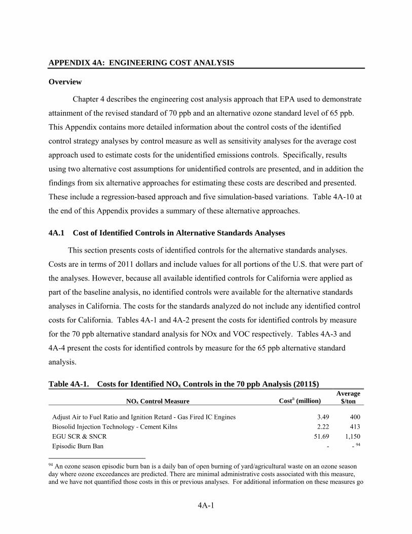
4A-1
APPENDIX 4A: ENGINEERING COST ANALYSIS
Overview
Chapter 4 describes the engineering cost analysis approach that EPA used to demonstrate
attainment of the revised standard of 70 ppb and an alternative ozone standard level of 65 ppb.
This Appendix contains more detailed information about the control costs of the identified
control strategy analyses by control measure as well as sensitivity analyses for the average cost
approach used to estimate costs for the unidentified emissions controls. Specifically, results
using two alternative cost assumptions for unidentified controls are presented, and in addition the
findings from six alternative approaches for estimating these costs are described and presented.
These include a regression-based approach and five simulation-based variations. Table 4A-10 at
the end of this Appendix provides a summary of these alternative approaches.
4A.1 Cost of Identified Controls in Alternative Standards Analyses
This section presents costs of identified controls for the alternative standards analyses.
Costs are in terms of 2011 dollars and include values for all portions of the U.S. that were part of
the analyses. However, because all available identified controls for California were applied as
part of the baseline analysis, no identified controls were available for the alternative standards
analyses in California. The costs for the standards analyzed do not include any identified control
costs for California. Tables 4A-1 and 4A-2 present the costs for identified controls by measure
for the 70 ppb alternative standard analysis for NOx and VOC respectively. Tables 4A-3 and
4A-4 present the costs for identified controls by measure for the 65 ppb alternative standard
analysis.
Table 4A-1. Costs for Identified NOx Controls in the 70 ppb Analysis (2011$)
NOx Control Measure Costa (million) Average
$/ton
Adjust Air to Fuel Ratio and Ignition Retard - Gas Fired IC Engines 3.49
400
Biosolid Injection Technology - Cement Kilns 2.22 413
EGU SCR & SNCR 51.69 1,150
Episodic Burn Ban - - 94
94 An ozone season episodic burn ban is a daily ban of open burning of yard/agricultural waste on an ozone season day where ozone exceedances are predicted. There are minimal administrative costs associated with this measure, and we have not quantified those costs in this or previous analyses. For additional information on these measures go

4A-2
NOx Control Measure Costa (million) Average
$/ton
Excess O3 Control 0.01 24
Ignition Retard - IC Engines 0.73 1,185
Low Emission Combustion - Gas Fired Lean Burn IC Engines 14.66 829
Low NOx Burner - Coal Cleaning 0.30 1,125
Low NOx Burner - Commercial/Institutional Boilers & IC Engines 23.78 1,110
Low NOx Burner - Gas-Fired Combustion 8.96 970
Low NOx Burner - Glass Manufacturing 0.28 1,141
Low NOx Burner - Industr/Commercial/Institutional (ICI) Boilers 6.33 1,135
Low NOx Burner - Industrial Combustion 0.03 1,255
Low NOx Burner - Lime Kilns 2.22 913
Low NOx Burner - Natural Gas-Fired Turbines 12.27 1,955
Low NOx Burner - Residential Water Heaters & Space Heaters 22.57
1,134
Low NOx Burner and Flue Gas Recirculation - Coke Oven/Blast Furnace 1.87 5,199
Low NOx Burner and Flue Gas Recirculation - Fluid Catalytic Cracking Units 0.17 2,091
Low NOx Burner and Flue Gas Recirculation - Iron & Steel 0.25 619
Low NOx Burner and SCR - Industr/Commercial/Institutional Boilers 62.83 7,473
Mid-Kiln Firing - Cement Manufacturing 0.09 73
Non-Selective Catalytic Reduction (NSCR) - 4 Cycle Rich Burn IC Engines 41.27 1,051
Nonroad Diesel Retrofits & Engine Rebuilds - e.g., Construction Equipment 12.87 4,545
OXY-Firing - Glass Manufacturing 44.23 3,691
Replacement of Residential & Commercial/Institutional Water Heaters -- --95
Selective Catalytic Reduction (SCR) - Cement Kilns 54.22 5,328
Selective Catalytic Reduction (SCR) - Fluid Catalytic Cracking Units 7.54 4,414
Selective Catalytic Reduction (SCR) - Glass Manufacturing 4.03 1,157
Selective Catalytic Reduction (SCR) - IC Engines, Diesel 3.29 3,814
Selective Catalytic Reduction (SCR) - ICI Boilers 17.35 3,756
Selective Catalytic Reduction (SCR) - Industrial Incinerators 5.27 3,805
Selective Catalytic Reduction (SCR) - Iron & Steel 0.80 5,180
Selective Catalytic Reduction (SCR) - Process Heaters 6.65 8,483
Selective Catalytic Reduction (SCR) - Sludge Incinerators 0.38 3,805
Selective Catalytic Reduction (SCR) - Space Heaters 0.11 4,661
Selective Catalytic Reduction (SCR) - Utility Boilers 0.18 128
Selective Non-Catalytic Reduction (SNCR) - Cement Manufacturing 3.13 1,303
Selective Non-Catalytic Reduction (SNCR) - Coke Manufacturing 4.25 2,673
Selective Non-Catalytic Reduction (SNCR) - Comm./Inst. Incinerators 0.11 1,842
Selective Non-Catalytic Reduction (SNCR) - Industrial Incinerators 0.60 1,645
Selective Non-Catalytic Reduction (SNCR) - Sludge Incinerators 0.06 1,842
to http://www.epa.gov/ttn/ecas/cost.htm. The EPA will continue to conduct research on possible costs for this measure, and if applicable update costs for this measure in future analyses. 95 We have not quantified specific costs for this measure in this or previous analyses. For additional information on these measures go to http://www.epa.gov/ttn/ecas/cost.htm. The EPA will continue to conduct research on possible costs for this measure, and if applicable update costs for this measure in future analyses.

4A-3
NOx Control Measure Costa (million) Average
$/ton
Ultra-Low NOx Burner - Process Heaters 0.14 420 a All values are rounded to two significant figures.
Table 4A-2. Costs for Identified VOC Controls in the 70 ppb Analysis (2011$)
VOC Control Measure Costa (million) Average $/ton
Control Technology Guidelines - Wood Furniture Surface Coating 8.87 32,595
Control of Fugitive Releases - Oil & Natural Gas Production 0.02 2,689
Flare - Petroleum Flare 0.31 3,305
Incineration - Other 155.85 14,543
LPV Relief Valve - Underground Tanks 2.29 1,763
MACT - Motor Vehicle Coating 0.00 192
Permanent Total Enclosure (PTE) - Surface Coating 4.53 12,289
RACT - Graphic Arts 1.66 6,386
Reduced Solvent Utilization - Surface Coating 0.03 1,232
Reformulation - Architectural Coatings 86.00 16,394
Reformulation - Pesticides Application 2.59 15,157
Reformulation-Process Modification - Automobile Refinishing 2.58 11,734
Reformulation-Process Modification - Cutback Asphalt 0.02 24
Reformulation-Process Modification - Other 0.35 3,102
Reformulation-Process Modification - Surface Coating 0.59 3,304
Solvent Recovery System - Printing/Publishing 0.02 1,232
Wastewater Treatment Controls- POTWs 0.70 3,366 a All values are rounded to two significant figures.
Table 4A-3. Costs for Identified NOx Controls in the 65 ppb Analysis (2011$) NOx Control Measure Costa (million) Average $/ton
Adjust Air to Fuel Ratio and Ignition Retard - Gas Fired IC Engines 7.25 441
Biosolid Injection Technology - Cement Kilns 2.44 413
EGU SCR & SNCR 125.93 1,150
Episodic Burn Ban - -96
Ignition Retard - IC Engines 0.73 1,262
Low Emission Combustion - Gas Fired Lean Burn IC Engines 57.85 764
Low NOx Burner - Coal Cleaning 0.69 1,451
Low NOx Burner - Commercial/Institutional Boilers & IC Engines 38.59 1,066
Low NOx Burner - Fiberglass Manufacturing 0.10 1,522
Low NOx Burner - Gas-Fired Combustion 11.53 970
Low NOx Burner - Industr/Commercial/Institutional (ICI) Boilers 56.57 2,581
96An ozone season episodic burn ban is a daily ban of open burning of yard/agricultural waste on an ozone season day where ozone exceedances are predicted. There are minimal administrative costs associated with this measure, and we have not quantified those costs in this or previous analyses. For additional information on these measures go to http://www.epa.gov/ttn/ecas/cost.htm. The EPA will continue to conduct research on possible costs for this measure, and if applicable update costs for this measure in future analyses.
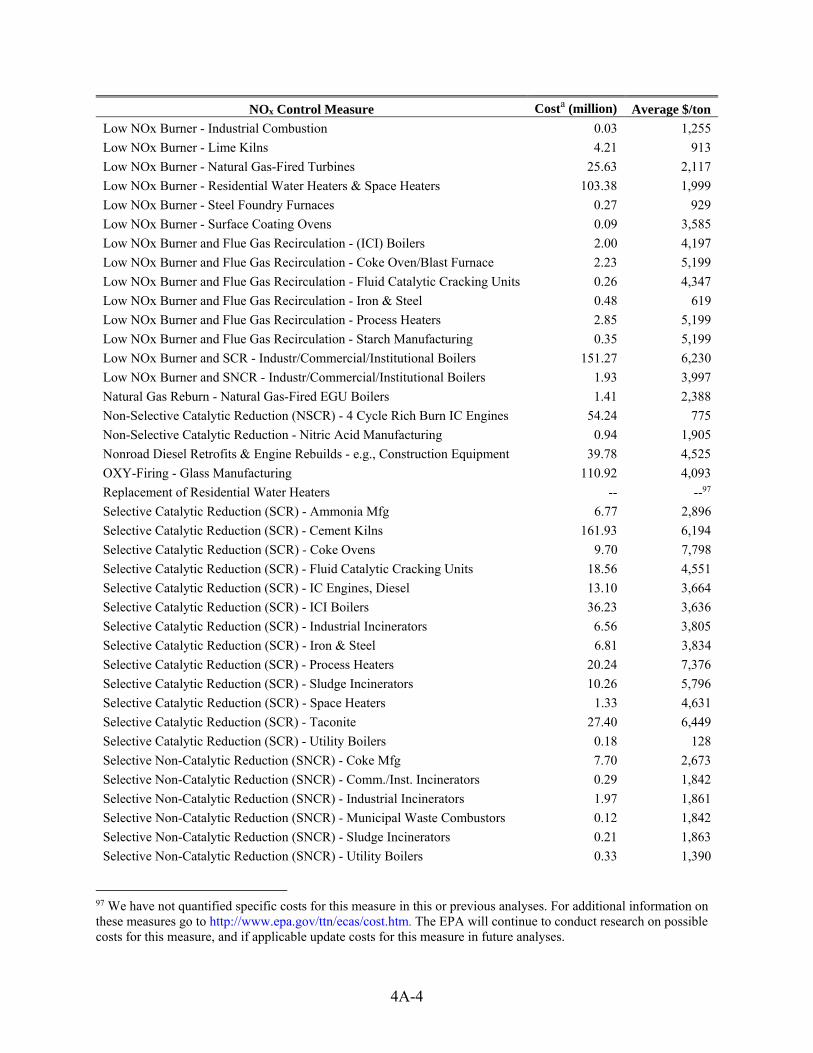
4A-4
NOx Control Measure Costa (million) Average $/ton
Low NOx Burner - Industrial Combustion 0.03 1,255
Low NOx Burner - Lime Kilns 4.21 913
Low NOx Burner - Natural Gas-Fired Turbines 25.63 2,117
Low NOx Burner - Residential Water Heaters & Space Heaters 103.38 1,999
Low NOx Burner - Steel Foundry Furnaces 0.27 929
Low NOx Burner - Surface Coating Ovens 0.09 3,585
Low NOx Burner and Flue Gas Recirculation - (ICI) Boilers 2.00 4,197
Low NOx Burner and Flue Gas Recirculation - Coke Oven/Blast Furnace 2.23 5,199
Low NOx Burner and Flue Gas Recirculation - Fluid Catalytic Cracking Units 0.26 4,347
Low NOx Burner and Flue Gas Recirculation - Iron & Steel 0.48 619
Low NOx Burner and Flue Gas Recirculation - Process Heaters 2.85 5,199
Low NOx Burner and Flue Gas Recirculation - Starch Manufacturing 0.35 5,199
Low NOx Burner and SCR - Industr/Commercial/Institutional Boilers 151.27 6,230
Low NOx Burner and SNCR - Industr/Commercial/Institutional Boilers 1.93 3,997
Natural Gas Reburn - Natural Gas-Fired EGU Boilers 1.41 2,388
Non-Selective Catalytic Reduction (NSCR) - 4 Cycle Rich Burn IC Engines 54.24 775
Non-Selective Catalytic Reduction - Nitric Acid Manufacturing 0.94 1,905
Nonroad Diesel Retrofits & Engine Rebuilds - e.g., Construction Equipment 39.78 4,525
OXY-Firing - Glass Manufacturing 110.92 4,093
Replacement of Residential Water Heaters -- --97
Selective Catalytic Reduction (SCR) - Ammonia Mfg 6.77 2,896
Selective Catalytic Reduction (SCR) - Cement Kilns 161.93 6,194
Selective Catalytic Reduction (SCR) - Coke Ovens 9.70 7,798
Selective Catalytic Reduction (SCR) - Fluid Catalytic Cracking Units 18.56 4,551
Selective Catalytic Reduction (SCR) - IC Engines, Diesel 13.10 3,664
Selective Catalytic Reduction (SCR) - ICI Boilers 36.23 3,636
Selective Catalytic Reduction (SCR) - Industrial Incinerators 6.56 3,805
Selective Catalytic Reduction (SCR) - Iron & Steel 6.81 3,834
Selective Catalytic Reduction (SCR) - Process Heaters 20.24 7,376
Selective Catalytic Reduction (SCR) - Sludge Incinerators 10.26 5,796
Selective Catalytic Reduction (SCR) - Space Heaters 1.33 4,631
Selective Catalytic Reduction (SCR) - Taconite 27.40 6,449
Selective Catalytic Reduction (SCR) - Utility Boilers 0.18 128
Selective Non-Catalytic Reduction (SNCR) - Coke Mfg 7.70 2,673
Selective Non-Catalytic Reduction (SNCR) - Comm./Inst. Incinerators 0.29 1,842
Selective Non-Catalytic Reduction (SNCR) - Industrial Incinerators 1.97 1,861
Selective Non-Catalytic Reduction (SNCR) - Municipal Waste Combustors 0.12 1,842
Selective Non-Catalytic Reduction (SNCR) - Sludge Incinerators 0.21 1,863
Selective Non-Catalytic Reduction (SNCR) - Utility Boilers 0.33 1,390
97 We have not quantified specific costs for this measure in this or previous analyses. For additional information on these measures go to http://www.epa.gov/ttn/ecas/cost.htm. The EPA will continue to conduct research on possible costs for this measure, and if applicable update costs for this measure in future analyses.

4A-5
NOx Control Measure Costa (million) Average $/ton
Ultra-Low NOx Burner - Process Heaters 1.24 1,447 a All values are rounded to two significant figures.
Table 4A-4. Costs for Identified VOC Controls in the 65 ppb Analysis (2011$)
VOC Control Measure Costa
(million) Average ($/ton)
Control Technology Guidelines - Wood Furniture Surface Coating 97.41 32,595
Control of Fugitive Releases - Oil & Natural Gas Production 0.08 2,689
Flare - Petroleum Flare 0.36 3,305
Gas Recovery - Municipal Solid Waste Landfill 0.32 1,106
Improved Work Practices, Material Substitution, Add-On Controls - Printing 0.00 159 Improved Work Practices, Material Substitution, Add-On Controls -Industrial Cleaning Solvents (0.34) (1,360)
Incineration - Other 240.54 14,395
LPV Relief Valve - Underground Tanks 8.59 1,763
Low VOC Adhesives and Improved Application Methods - Industrial Adhesives 0.06 270
Low-VOC Coatings and Add-On Controls - Surface Coating 0.73 2,668
MACT - Motor Vehicle Coating 0.37 192
Permanent Total Enclosure (PTE) - Surface Coating 45.92 13,973
Petroleum and Solvent Evaporation - Surface Coating Operations 0.09 376
RACT - Graphic Arts 35.67 6,386
Reduced Solvent Utilization - Surface Coating 5.36 1,758
Reformulation - Architectural Coatings 858.67 16,394
Reformulation - Industrial Adhesives 13.34 12,017
Reformulation - Pesticides Application 59.97 15,157
Reformulation-Process Modification - Automobile Refinishing 57.25 11,734
Reformulation-Process Modification - Cutback Asphalt 0.06 24
Reformulation-Process Modification - Oil & Natural Gas Production 0.19 641
Reformulation-Process Modification - Other 1.94 3,548
Reformulation-Process Modification - Surface Coating 21.00 3,736
Solvent Recovery System - Printing/Publishing 1.05 1,232
Solvent Substitution and Improved Application Methods - Fiberglass Boat Mfg 0.06 4,310
Wastewater Treatment Controls- POTWs 0.79 3,366 a All values are rounded to two significant figures.
4A.2 Alternative Estimates of Costs Associated with Emissions Reductions from Unidentified Controls
This section presents alternative estimates of the unidentified control costs using
alternative average cost per ton of emissions reductions from unidentified controls of $10,000
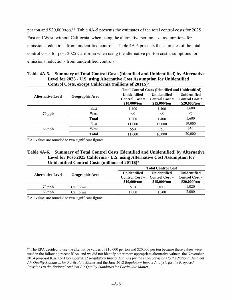
4A-6
per ton and $20,000/ton.98 Table 4A-5 presents the estimates of the total control costs for 2025
East and West, without California, when using the alternative per ton cost assumptions for
emissions reductions from unidentified controls. Table 4A-6 presents the estimates of the total
control costs for post-2025 California when using the alternative per ton cost assumptions for
emissions reductions from unidentified controls.
Table 4A-5. Summary of Total Control Costs (Identified and Unidentified) by Alternative Level for 2025 - U.S. using Alternative Cost Assumption for Unidentified Control Costs, except California (millions of 2011$)a
Alternative Level Geographic Area
Total Control Costs (Identified and Unidentified) Unidentified
Control Cost = $10,000/ton
Unidentified Control Cost =
$15,000/ton
Unidentified Control Cost =
$20,000/ton
70 ppb East 1,100 1,400 1,600
West <5 <5 <5
Total 1,200 1,400 1,600
65 ppb East 11,000 15,000 19,000
West 550 750 950
Total 11,000 16,000 20,000 a All values are rounded to two significant figures.
Table 4A-6. Summary of Total Control Costs (Identified and Unidentified) by Alternative Level for Post-2025 California - U.S. using Alternative Cost Assumption for Unidentified Control Costs (millions of 2011$)a
Alternative Level Geographic Area
Total Control Cost Unidentified
Control Cost = $10,000/ton
Unidentified Control Cost =
$15,000/ton
Unidentified Control Cost =
$20,000/ton 70 ppb California 510 800 1,020
65 ppb California 1,000 1,500 2,000 a All values are rounded to two significant figures.
98 The EPA decided to use the alternative values of $10,000 per ton and $20,000 per ton because these values were used in the following recent RIAs, and we did not identify other more appropriate alternative values: the November 2014 proposal RIA, the December 2012 Regulatory Impact Analysis for the Final Revisions to the National Ambient Air Quality Standards for Particulate Matter and the June 2012 Regulatory Impact Analysis for the Proposed Revisions to the National Ambient Air Quality Standards for Particulate Matter.
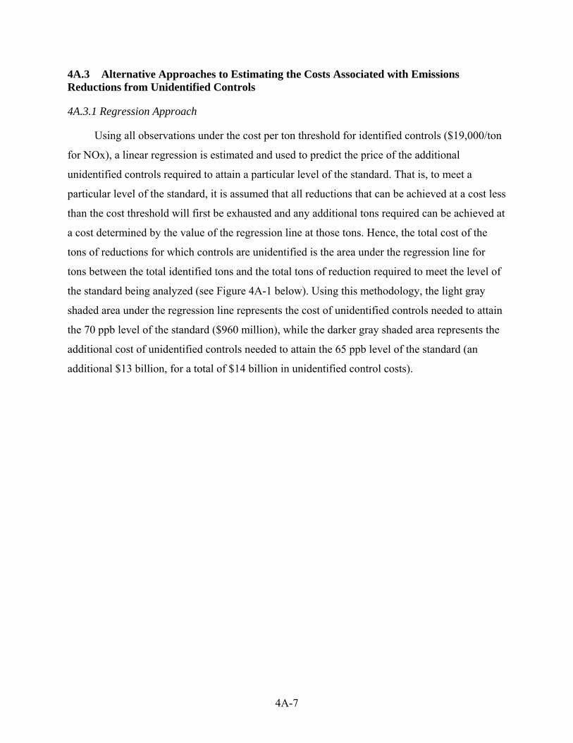
4A-7
4A.3 Alternative Approaches to Estimating the Costs Associated with Emissions Reductions from Unidentified Controls
4A.3.1 Regression Approach
Using all observations under the cost per ton threshold for identified controls ($19,000/ton
for NOx), a linear regression is estimated and used to predict the price of the additional
unidentified controls required to attain a particular level of the standard. That is, to meet a
particular level of the standard, it is assumed that all reductions that can be achieved at a cost less
than the cost threshold will first be exhausted and any additional tons required can be achieved at
a cost determined by the value of the regression line at those tons. Hence, the total cost of the
tons of reductions for which controls are unidentified is the area under the regression line for
tons between the total identified tons and the total tons of reduction required to meet the level of
the standard being analyzed (see Figure 4A-1 below). Using this methodology, the light gray
shaded area under the regression line represents the cost of unidentified controls needed to attain
the 70 ppb level of the standard ($960 million), while the darker gray shaded area represents the
additional cost of unidentified controls needed to attain the 65 ppb level of the standard (an
additional $13 billion, for a total of $14 billion in unidentified control costs).
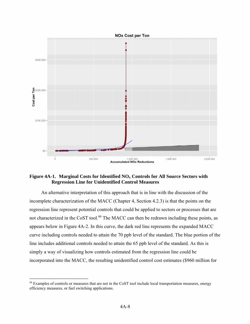
4A-8
Figure 4A-1. Marginal Costs for Identified NOx Controls for All Source Sectors with Regression Line for Unidentified Control Measures
An alternative interpretation of this approach that is in line with the discussion of the
incomplete characterization of the MACC (Chapter 4, Section 4.2.3) is that the points on the
regression line represent potential controls that could be applied to sectors or processes that are
not characterized in the CoST tool.99 The MACC can then be redrawn including these points, as
appears below in Figure 4A-2. In this curve, the dark red line represents the expanded MACC
curve including controls needed to attain the 70 ppb level of the standard. The blue portion of the
line includes additional controls needed to attain the 65 ppb level of the standard. As this is
simply a way of visualizing how controls estimated from the regression line could be
incorporated into the MACC, the resulting unidentified control cost estimates ($960 million for
99 Examples of controls or measures that are not in the CoST tool include local transportation measures, energy efficiency measures, or fuel switching applications.
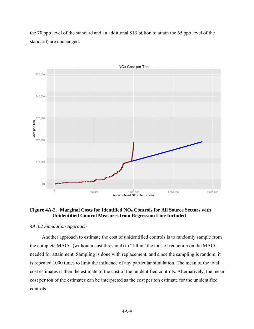
4A-9
the 70 ppb level of the standard and an additional $13 billion to attain the 65 ppb level of the
standard) are unchanged.
Figure 4A-2. Marginal Costs for Identified NOx Controls for All Source Sectors with Unidentified Control Measures from Regression Line Included
4A.3.2 Simulation Approach
Another approach to estimate the cost of unidentified controls is to randomly sample from
the complete MACC (without a cost threshold) to “fill in” the tons of reduction on the MACC
needed for attainment. Sampling is done with replacement, and since the sampling is random, it
is repeated 1000 times to limit the influence of any particular simulation. The mean of the total
cost estimates is then the estimate of the cost of the unidentified controls. Alternatively, the mean
cost per ton of the estimates can be interpreted as the cost per ton estimate for the unidentified
controls.

4A-10
The implicit assumption when applying this simulation approach is that the controls in the
incomplete MACC curve are representative of the types of controls (both in cost and
effectiveness) that could be applied to alternative sources not yet controlled or adequately
characterized in the CoST database, and also that controls that may be developed in the future
(prior to the attainment date) will be similar in cost and effectiveness to controls currently
available. While we do not believe that controls with costs greater than the cost threshold are
likely to be applied, they are not removed from the simulation dataset in order to provide a more
complete set of identified abatement possibilities.
The CoST database used for this analysis contains approximately 120,000 individual
controls applicable to five broad sectors. While there is geographic specificity in the applicability
of the controls, the simulation is currently being performed on a national scale. The cost per ton
and number of available controls differs considerably between sectors, as shown below in Table
4A-7, and for this reason it is important to determine how broadly to sample when selecting
controls to attain a particular level of the standard.
Table 4A-7. Costs and Number of Identified NOx Controls by Sector in the CoST Database (2011$)
Sector
Number of
Controls
Cost per Ton
Minimum Median Mean Maximum
nonpt 2,069 $413 $1,008 $1,455 $2,005
nonroad 111,943 $3,330 $4,618 $4,619 $5,300
np_oilgas 772 $78 $649 $747 $2,019
pt_oilgas 3,892 $12 $649 $1,120 $44,860
ptnonipm 2,756 $18 $3,814 $12,147 $354,974
In this simulation approach, we investigate three methods for selecting available controls
to expand the MACC to simulate attainment. First, the sectors are aggregated into three broad
sectors (nonroad, nonpoint, and non-EGU point sources) and controls are selected from these
sectors in the same proportion as the control strategy discussed in Chapter 3 for these three
sectors for each level of the standard. These percentages appear below in Table 4A-8.
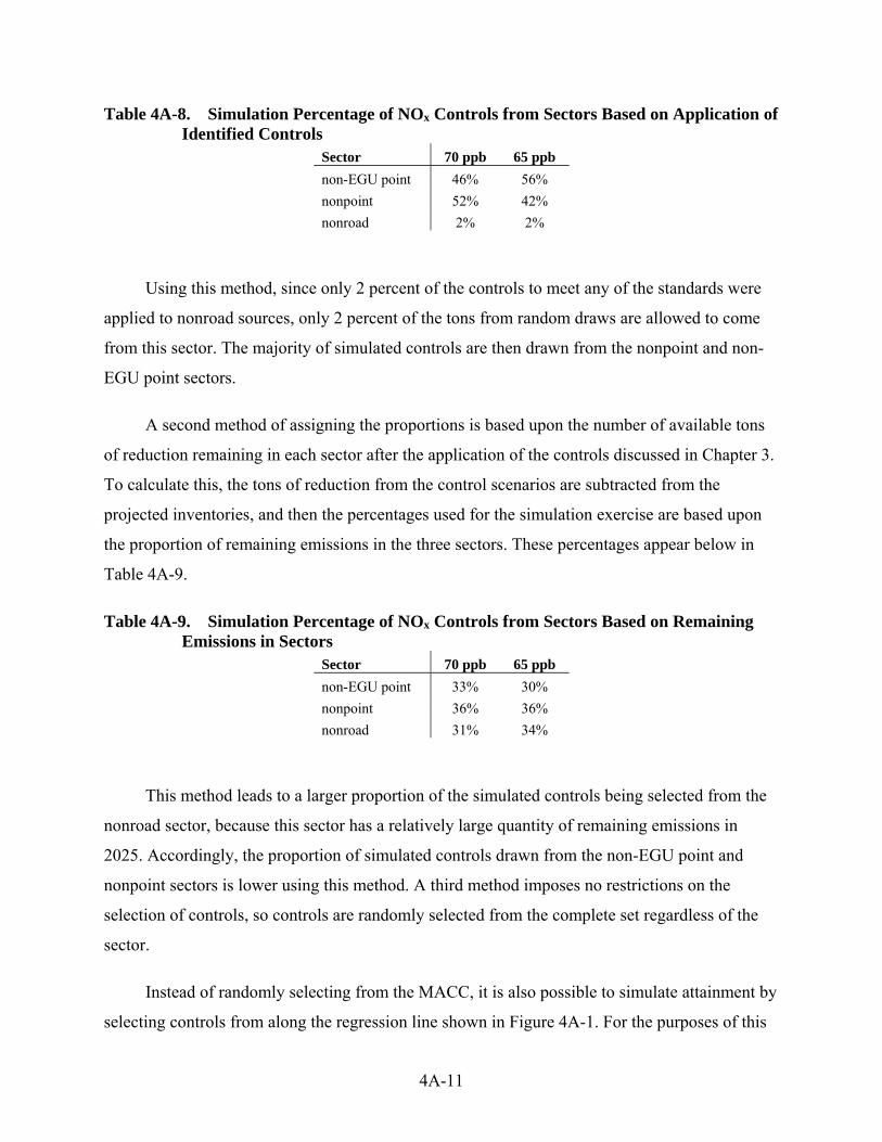
4A-11
Table 4A-8. Simulation Percentage of NOx Controls from Sectors Based on Application of Identified Controls
Sector 70 ppb 65 ppb
non-EGU point 46% 56%
nonpoint 52% 42%
nonroad 2% 2%
Using this method, since only 2 percent of the controls to meet any of the standards were
applied to nonroad sources, only 2 percent of the tons from random draws are allowed to come
from this sector. The majority of simulated controls are then drawn from the nonpoint and non-
EGU point sectors.
A second method of assigning the proportions is based upon the number of available tons
of reduction remaining in each sector after the application of the controls discussed in Chapter 3.
To calculate this, the tons of reduction from the control scenarios are subtracted from the
projected inventories, and then the percentages used for the simulation exercise are based upon
the proportion of remaining emissions in the three sectors. These percentages appear below in
Table 4A-9.
Table 4A-9. Simulation Percentage of NOx Controls from Sectors Based on Remaining Emissions in Sectors
Sector 70 ppb 65 ppb
non-EGU point 33% 30%
nonpoint 36% 36%
nonroad 31% 34%
This method leads to a larger proportion of the simulated controls being selected from the
nonroad sector, because this sector has a relatively large quantity of remaining emissions in
2025. Accordingly, the proportion of simulated controls drawn from the non-EGU point and
nonpoint sectors is lower using this method. A third method imposes no restrictions on the
selection of controls, so controls are randomly selected from the complete set regardless of the
sector.
Instead of randomly selecting from the MACC, it is also possible to simulate attainment by
selecting controls from along the regression line shown in Figure 4A-1. For the purposes of this
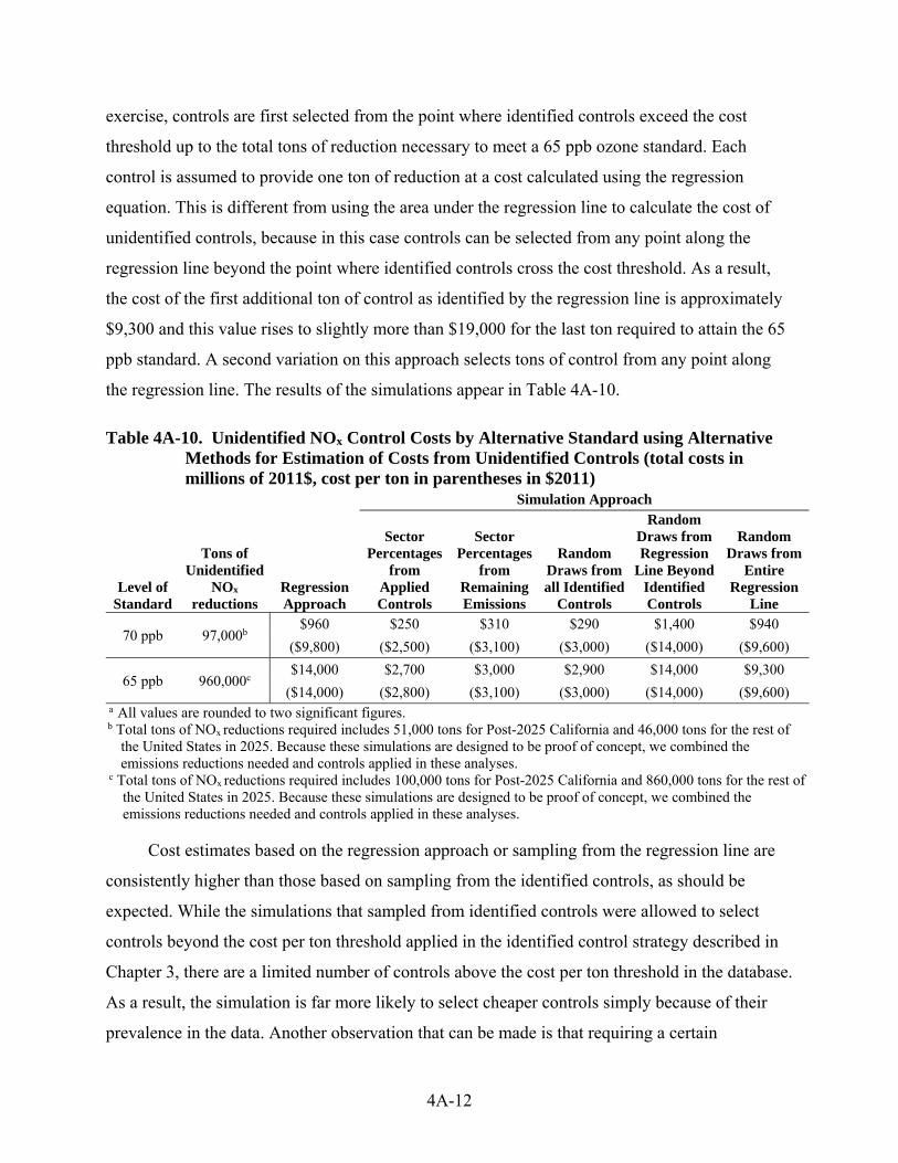
4A-12
exercise, controls are first selected from the point where identified controls exceed the cost
threshold up to the total tons of reduction necessary to meet a 65 ppb ozone standard. Each
control is assumed to provide one ton of reduction at a cost calculated using the regression
equation. This is different from using the area under the regression line to calculate the cost of
unidentified controls, because in this case controls can be selected from any point along the
regression line beyond the point where identified controls cross the cost threshold. As a result,
the cost of the first additional ton of control as identified by the regression line is approximately
$9,300 and this value rises to slightly more than $19,000 for the last ton required to attain the 65
ppb standard. A second variation on this approach selects tons of control from any point along
the regression line. The results of the simulations appear in Table 4A-10.
Table 4A-10. Unidentified NOx Control Costs by Alternative Standard using Alternative Methods for Estimation of Costs from Unidentified Controls (total costs in millions of 2011$, cost per ton in parentheses in $2011)
Level of
Standard
Tons of Unidentified
NOx reductions
Regression Approach
Simulation Approach
Sector Percentages
from Applied Controls
Sector Percentages
from Remaining Emissions
Random Draws from all Identified
Controls
Random Draws from Regression
Line Beyond Identified Controls
Random Draws from
Entire Regression
Line
70 ppb 97,000b $960 $250 $310 $290 $1,400 $940
($9,800) ($2,500) ($3,100) ($3,000) ($14,000) ($9,600)
65 ppb 960,000c $14,000 $2,700 $3,000 $2,900 $14,000 $9,300
($14,000) ($2,800) ($3,100) ($3,000) ($14,000) ($9,600) a All values are rounded to two significant figures. b Total tons of NOx reductions required includes 51,000 tons for Post-2025 California and 46,000 tons for the rest of
the United States in 2025. Because these simulations are designed to be proof of concept, we combined the emissions reductions needed and controls applied in these analyses.
c Total tons of NOx reductions required includes 100,000 tons for Post-2025 California and 860,000 tons for the rest of the United States in 2025. Because these simulations are designed to be proof of concept, we combined the emissions reductions needed and controls applied in these analyses.
Cost estimates based on the regression approach or sampling from the regression line are
consistently higher than those based on sampling from the identified controls, as should be
expected. While the simulations that sampled from identified controls were allowed to select
controls beyond the cost per ton threshold applied in the identified control strategy described in
Chapter 3, there are a limited number of controls above the cost per ton threshold in the database.
As a result, the simulation is far more likely to select cheaper controls simply because of their
prevalence in the data. Another observation that can be made is that requiring a certain

4A-13
percentage of controls from particular sectors does affect the results, but not to the extent that
might be expected. While the cost of controls vary between sectors, the simulations produced
similar results regardless of restrictions on the distribution of controls across sectors. Finally,
while the cost per ton estimates varied considerably across the approaches, all cost per ton
estimates were below the $15,000/ton estimate used as the primary estimate of the cost of
unidentified controls.
The EPA continues to investigate methods to better estimate the cost of currently
unidentified controls. While we have reason to believe that technological advances over the
coming years will both lead to new types of controls as well as reduce the cost of currently
available controls, we do not presently possess the capability to accurately predict the rate at
which technological progress will occur or the potential impacts such progress will have on the
cost of controls. As a result, the simulations presented herein draw upon currently identified
controls and their current costs, or a linear regression of these data. The results of the simulations
are sensitive to the percentage of unidentified controls required from each sector, and for this
reason we plan to continue investigating methods for assigning these percentages based upon the
degree to which sectors have already been controlled. Furthermore, while the simulations in this
appendix were performed at the national level, we recognize that areas differ greatly in their
industrial base, and for this reason the simulations should be performed at a more disaggregated
level using data about the emissions sources in each area, available controls, and the degree to
which sources in the area have already been controlled. Because these simulations are designed
to be proof of concept, we combined the emissions reductions needed and controls applied in
these analyses.
5-1
CHAPTER 5: QUALITATIVE DISCUSSION OF EMPLOYMENT IMPACTS OF AIR QUALITY
Overview
Executive Order 13563 directs federal agencies to consider regulatory impacts on job
creation and employment. According to the Executive Order, “our regulatory system must
protect public health, welfare, safety, and our environment while promoting economic growth,
innovation, competitiveness, and job creation. It must be based on the best available science”
(Executive Order 13563, 2011). Although standard benefit-cost analyses have not typically
included a separate analysis of regulation-induced employment impacts,100 we typically conduct
employment analyses for economically significant rules. While the economy continues moving
toward full employment, employment impacts are of particular concern and questions may arise
about their existence and magnitude. This chapter discusses some, but not all, possible types of
labor impacts that may result from measures to decrease NOx emissions.101
Section 5.1 describes the theoretical framework used to analyze regulation-induced
employment impacts, discussing how economic theory alone cannot predict whether such
impacts are positive or negative. Section 5.2 presents an overview of the peer-reviewed literature
relevant to evaluating the effect of environmental regulation on employment. Section 5.3
discusses employment related to installation of NOx controls on coal and gas-fired electric
generating units, industrial boilers, and cement kilns.
5.1 Economic Theory and Employment
Regulatory employment impacts are difficult to disentangle from other economic changes
affecting employment decisions over time and across regions and industries. Labor market
responses to regulation are complex. They depend on labor demand and supply elasticities and
possible labor market imperfections (e.g., wage stickiness, long-term unemployment, etc). The
unit of measurement (e.g., number of jobs, types of job hours worked, and earnings) may affect
observability of that response. Net employment impacts are composed of a mix of potential
100 Labor expenses do, however, contribute toward total costs in the EPA’s standard benefit-cost analyses. 101 The employment analysis in this RIA is part of EPA’s ongoing effort to “conduct continuing evaluations of potential loss or shifts of employment which may result from the administration or enforcement of [the Act]” pursuant to CAA section 321(a).

5-2
declines and gains in different areas of the economy (the directly regulated sector, upstream and
downstream sectors, etc.) over time. In light of these difficulties, economic theory provides a
constructive framework for analysis.
Microeconomic theory describes how firms adjust input use in response to changes in
economic conditions.102 Labor is one of many inputs to production, along with capital, energy,
and materials. In competitive markets, firms choose inputs and outputs to maximize profit as a
function of market prices and technological constraints.103,104
Berman and Bui (2001) adapt this model to analyze how environmental regulations affect
labor demand.105 They model environmental regulation as effectively requiring certain factors of
production, such as pollution abatement capital, at levels that firms would not otherwise choose.
Berman and Bui (2001) model two components that drive changes in firm-level labor
demand: output effects and substitution effects.106 Regulation affects the profit-maximizing
quantity of output by changing the marginal cost of production. If regulation causes marginal
cost to increase, it will place upward pressure on output prices, leading to a decrease in demand,
and resulting in a decrease in production. The output effect describes how, holding labor
intensity constant, a decrease in production causes a decrease in labor demand. As noted by
Berman and Bui, although many assume that regulation increases marginal cost, it need not be
the case. A regulation could induce a firm to upgrade to less polluting and more efficient
equipment that lowers marginal production costs. In such a case, output could increase for
facilities that do not exit the industry. For example, improving the heat rate of a utility boiler
increases fuel efficiency, lowering marginal production costs, and thereby potentially increasing
the boiler’s generation. An unregulated profit-maximizing firm may not have chosen to install
such an efficiency-improving technology if the investment cost were too high.
102 See Layard and Walters (1978), a standard microeconomic theory textbook, for a discussion, in Chapter 9. 103 See Hamermesh (1993), Ch. 2, for a derivation of the firm’s labor demand function from cost-minimization. 104 In this framework, labor demand is a function of quantity of output and prices (of both outputs and inputs). 105 Morgenstern, Pizer, and Shih (2002) develop a similar model. 106 The authors also discuss a third component, the impact of regulation on factor prices, but conclude that this effect is unlikely to be important for large competitive factor markets, such as labor and capital. Morgenstern, Pizer and Shih (2002) use a very similar model, but they break the employment effect into three parts: 1) a demand effect; 2) a cost effect; and 3) a factor-shift effect.
5-3
The substitution effect describes how, holding output constant, regulation affects labor-
intensity of production. Although stricter environmental regulation may increase use of pollution
control equipment and energy to operate that equipment, the impact on labor demand is
ambiguous. Equipment inspection requirements, specialized waste handling, or pollution
technologies that alter the production process may affect the number of workers necessary to
produce a unit of output. Berman and Bui (2001) model the substitution effect as the effect of
regulation on pollution control equipment and expenditures required by the regulation and the
corresponding change in labor-intensity of production.
In summary, as output and substitution effects may be positive or negative, theory cannot
predict the direction of the net effect of regulation on labor demand at the level of the regulated
firm. Operating within the bounds of standard economic theory, however, empirical estimation
of net employment effects on regulated firms is possible when data and methods of sufficient
detail and quality are available. The literature, however, illustrates difficulties with empirical
estimation. For example, studies sometimes rely on confidential plant-level employment data
from the U.S. Census Bureau, possibly combined with pollution abatement expenditure data that
are too dated to be reliably informative. In addition, the most commonly used empirical methods,
for example Greenstone (2002), likely overstate employment impacts because they rely on
relative comparisons between more regulated and less regulated counties, which can lead to
“double counting” of impacts when production and employment shift from more regulated
toward less regulated areas. Thus the empirical methods cannot be used to estimate net
employment effects.107
The conceptual framework described thus far focused on regulatory effects on plant-level
decisions within a regulated industry. Employment impacts at an individual plant do not
necessarily represent impacts for the sector as a whole. The approach must be modified when
applied at the industry level.
At the industry-level, labor demand is more responsive if: (1) the price elasticity of
demand for the product is high, (2) other factors of production can be easily substituted for labor,
107 See Greenstone (2002) p. 1212.

5-4
(3) the supply of other factors is highly elastic, or (4) labor costs are a large share of total
production costs.108 For example, if all firms in an industry are faced with the same regulatory
compliance costs and product demand is inelastic, then industry output may not change much,
and output of individual firms may change slightly.109 In this case the output effect may be small,
while the substitution effect depends on input substitutability. Suppose, for example, that new
equipment for heat rate improvements requires labor to install and operate. In this case the
substitution effect may be positive, and with a small output effect, the total effect may be
positive. As with potential effects for an individual firm, theory cannot determine the sign or
magnitude of industry-level regulatory effects on labor demand. Determining these signs and
magnitudes requires additional sector-specific empirical study. For environmental rules, much of
the data needed for these empirical studies are not publicly available, would require significant
time and resources in order to access confidential U.S. Census data for research, and also would
not be necessary for other components of a typical regulatory impact analysis (RIA).
In addition to changes to labor demand in the regulated industry, net employment impacts
encompass changes in other related sectors. For example, the proposed guidelines may increase
demand for pollution control equipment and services. This increased demand may increase
revenue and employment in the firms supporting this technology. At the same time, the regulated
industry is purchasing the equipment and these costs may impact labor demand at regulated
firms. Therefore, it is important to consider the net effect of compliance actions on employment
across multiple sectors or industries.
If the U.S. economy is at full employment, even a large-scale environmental regulation is
unlikely to have a noticeable impact on aggregate net national employment.110 Instead, labor
would primarily be reallocated from one productive use to another (e.g., from producing
electricity or steel to producing high efficiency equipment), and net national employment effects
108 See Ehrenberg & Smith, p. 108. 109 This discussion draws from Berman and Bui (2001), pp. 293. 110 Full employment is a conceptual target for the economy where everyone who wants to work and is available to do so at prevailing wages is actively employed. The unemployment rate at full employment is not zero.

5-5
from environmental regulation would be small and transitory (e.g., as workers move from one
job to another).111
Affected sectors may experience transitory effects as workers change jobs. Some workers
may retrain or relocate in anticipation of new requirements or require time to search for new
jobs, while shortages in some sectors or regions could bid up wages to attract workers. These
adjustment costs can lead to local labor disruptions. Although the net change in the national
workforce is expected to be small, localized reductions in employment may adversely impact
individuals and communities just as localized increases may have positive impacts.
If the economy is operating at less than full employment, economic theory does not clearly
indicate the direction or magnitude of the net impact of environmental regulation on
employment; it could cause either a short-run net increase or short-run net decrease
(Schmalansee and Stavins, 2011). For example, the Congressional Budget Office considered
EPA’s Mercury and Air Toxics Standards and regulations for industrial boilers and process
heaters as potentially leading to short-run net increases in economic growth and employment,
driven by capital investments for compliance with the regulations (Congressional Budget Office,
2011). An important research question is how to accommodate unemployment as a structural
feature in economic models. This feature may be important in assessing large-scale regulatory
impacts on employment (Smith 2012).
Environmental regulation may also affect labor supply. In particular, pollution and other
environmental risks may impact labor productivity or employees’ ability to work.112 While the
theoretical framework for analyzing labor supply effects is analogous to that for labor demand, it
is more difficult to study empirically. There is a small emerging literature, described in the next
section that uses detailed labor and environmental data to assess these impacts.
To summarize, economic theory provides a framework for analyzing the impacts of
environmental regulation on employment. The net employment effect incorporates expected
employment changes (both positive and negative) in the regulated sector and elsewhere. Labor
111 Arrow et. al. 1996; see discussion on bottom of p. 8. In practice, distributional impacts on individual workers can be important, as discussed in later paragraphs of this section. 112 E.g. Graff Zivin and Neidell (2012).

5-6
demand impacts for regulated firms, and also for the regulated industry, can be decomposed into
output and substitution effects which may be either negative or positive. Estimation of net
employment effects for regulated sectors is possible when data of sufficient detail and quality are
available. Finally, economic theory suggests that labor supply effects are also possible. In the
next section, we discuss the empirical literature.
5.2 Current State of Knowledge Based on the Peer-Reviewed Literature
The labor economics literature contains an extensive body of peer-reviewed empirical
work analyzing various aspects of labor demand, relying on the theoretical framework discussed
in the preceding section.113 This work focuses primarily on effects of employment policies such
as labor taxes and minimum wages.114 In contrast, the peer-reviewed empirical literature
specifically estimating employment effects of environmental regulations is more limited.
Empirical studies, such as Berman and Bui (2001) and Ferris, Shadbegian, and Wolverton
(2014), suggest that regulation-induced net employment impacts may be zero or slightly positive,
but small in the regulated sector. Other research on regulated sectors suggests that employment
growth may be lower in more regulated areas (Greenstone 2002, Walker 2011, 2013). However
since these latter studies compare more regulated to less regulated counties, this methodological
approach likely overstates employment impacts to the extent that regulation causes plants to
locate in one area of the country rather than another, which would lead to “double counting” of
the employment impacts. List et al. (2003) find some evidence that this type of geographic
relocation may be occurring. Environmental regulations may affect sectors that support
pollution reduction earlier than the regulated industry. Rules are usually announced well in
advance of their effective dates and then typically provide a period of time for firms to invest in
technologies and process changes to meet the new requirements. When a regulation is
promulgated, the initial response of firms is often to order pollution control equipment and
services to enable compliance when the regulation becomes effective. Estimates of short-term
increases in demand for specialized labor within the environmental protection sector have been
prepared for several EPA regulations in the past, including the Mercury and Air Toxics
113 Again, see Hamermesh (1993) for a detailed treatment. 114 See Ehrenberg & Smith (2000), Chapter 4: “Employment Effects: Empirical Estimates” for a concise overview.
5-7
Standards (MATS).115 Overall, the peer-reviewed literature does not contain evidence that
environmental regulation has a large impact on net employment (either negative or positive) in
the long run across the whole economy.
5.2.1 Regulated Sectors
Berman and Bui (2001) examine how an increase in local air quality regulation affects
manufacturing employment in the South Coast Air Quality Management District (SCAQMD),
which includes Los Angeles and its suburbs. From 1979 to 1992 the SCAQMD enacted some of
the country’s most stringent air quality regulations. Using SCAQMD’s local air quality
regulations, Berman and Bui identify the effect of environmental regulations on net employment
in regulated manufacturing industries relative to other plants in the same 4-digit SIC industries
but in regions not subject to local regulations.116 The authors find that “while regulations do
impose large costs, they have a limited effect on employment” (Berman and Bui, 2001, p. 269).
Their conclusion is that local air quality regulation “probably increased labor demand slightly”
but that “the employment effects of both compliance and increased stringency are fairly precisely
estimated zeros, even when exit and dissuaded entry effects are included” (Berman and Bui,
2001, p. 269).117
A small literature examines impacts of environmental regulations on manufacturing
employment. Greenstone (2002) and Walker (2011, 2013) study the impact of air quality
regulations on manufacturing employment, estimating the net effects in nonattainment areas
relative to attainment areas. Kahn and Mansur (2013) study environmental regulatory impacts on
geographic distribution of manufacturing employment, controlling for electricity prices and labor
regulation (right to work laws). Their methodology identifies employment impacts by focusing
on neighboring counties with different ozone regulations. They find limited evidence that
environmental regulations may cause employment to be lower within “county-border-pairs.”
This result suggests that regulation may cause an effective relocation of labor across a county
border, but since one county’s loss may be another’s gain, such shifts cannot be transformed into
115 U.S. EPA (2011b). 116 Berman and Bui include over 40 4-digit SIC industries in their sample. They do not estimate the number of jobs created in the environmental protection sector. 117 Including the employment effect of existing plants and plants dissuaded from opening will increase the estimated impact of regulation on employment.

5-8
an estimate of a national net effect on employment. Moreover this result is sensitive to model
specification choices.
5.2.2 Economy-Wide
As noted above it is very difficult to estimate the net national employment impacts of
environmental regulation. Given the difficulty with estimating national impacts of regulations,
EPA has not generally estimated economy-wide employment impacts of its regulations in its
benefit-cost analyses. However, in its continuing effort to advance the evaluation of costs,
benefits, and economic impacts associated with environmental regulation, EPA has formed a
panel of experts as part of EPA’s Science Advisory Board (SAB) to advise EPA on the technical
merits and challenges of using economy-wide economic models to evaluate the impacts of its
regulations, including the impact on net national employment.118 Once EPA receives guidance
from this panel it will carefully consider this input and then decide if and how to proceed on
economy-wide modeling of employment impacts of its regulations.
5.2.3 Labor Supply Impacts
The empirical literature on environmental regulatory employment impacts focuses
primarily on labor demand. However, there is a nascent literature focusing on regulation-induced
effects on labor supply.119 Although this literature is limited by empirical challenges, researchers
have found that air quality improvements lead to reductions in lost work days (e.g., Ostro 1987).
Limited evidence suggests worker productivity may also improve when pollution is reduced.
Graff Zivin and Neidell (2012) used detailed worker-level productivity data from 2009 and 2010,
paired with local ozone air quality monitoring data for one large California farm growing
multiple crops, with a piece-rate payment structure. Their quasi-experimental structure identifies
an effect of daily variation in monitored ozone levels on productivity. They find “ozone levels
well below federal air quality standards have a significant impact on productivity: a 10 parts per
118 For further information see: http://yosemite.epa.gov/sab/sabproduct.nsf/0/07E67CF77B54734285257BB0004F87ED?OpenDocument 119 For a recent review see Graff-Zivin and Neidell (2013).

5-9
billion (ppb) decreases in ozone concentrations increases worker productivity by 5.5 percent.”
(Graff Zivin and Neidell, 2012, p. 3654).120
This section has outlined the challenges associated with estimating regulatory effects on
both labor demand and supply for specific sectors. These challenges make it difficult to estimate
net national employment estimates that would appropriately capture the way in which costs,
compliance spending, and environmental benefits propagate through the macro-economy.
5.3 Employment Related to Installation and Maintenance of NOx Control Equipment
This section discusses employment related to installation of NOx controls on coal and
gas-fired electric generating units (EGUs), industrial boilers, and cement kilns, which are among
the highest NOx-emitting source categories in EPA’s emissions inventory (see Chapter 2 and
Appendix 2A for more detail on emissions). The employment analysis in this section is an
illustrative analysis, estimating the amount of labor involved with installing advanced NOx
emission control systems at each of these three different types of NOx emission sources. The
analysis also estimates the labor needed to operate existing advanced NOx systems more
frequently (e.g., year round). Sections 5.3.1 and 5.3.2 below contain estimates of the number of
direct short-term and long-term jobs that would be created by addition of NOx controls at a
single facility (or unit) in each of these three categories of emissions sources, for various size
units. Because the apportionment of emissions control across emissions sources in this RIA
analysis is an illustrative model plant analysis, and is not necessarily representative of the
controls that will be required in individual state SIPs, the EPA did not estimate short-term or
long-term employment that would result from addition of NOx controls at these three source
categories either everywhere throughout the country, or at facilities located in areas anticipated
to need additional NOx reductions for the 65 ppb and 70 ppb standard alternatives.
5.3.1 Employment Resulting from Addition of NOx Controls at EGUs
This section presents an illustrative analysis of the direct labor needs to install and
operate SCRs at three common sizes of coal-fired EGUs: 300 MW, 500 MW and 1000 MW. As
120 The EPA is not quantifying productivity impacts of reduced pollution in this rulemaking using this study. In light of this recent research, however, the EPA is considering how best to incorporate possible productivity effects in the future.

5-10
discussed below, the illustrative analysis is for a “model plant” of each size, using consistent
assumptions about the plant’s operation that impact the material and labor needs of a
representative plant, such as the capacity factor, heat rate, and type of coal. The analysis does not
include an estimate of the aggregate total of the labor needed for installing and running SCRs at
any particular level of the revised ozone standard; nor does it reflect plant-specific variations in
labor needs due to regional differences in prices and labor availability, existing control
technology at the plant, etc.
Coal-fired EGUs are likely to apply additional NOx controls in response to State
Implementation Plans (SIPs) approved pursuant to a revised ozone standard. While many EGUs
have already installed and operate various NOx control devices, there are additional existing
coal-fired EGUs that could further decrease NOx emissions by either (a) upgrading or replacing
their existing NOx emissions reducing systems, or (b) operating their existing NOx systems for
more hours in the year than the IPM model predicts they will in the IPM v. 5.14 base case121 for
2025. While all existing coal-fired EGUs already have low NOx burners, there are EGUs that
currently have a selective non-catalytic reduction (SNCR) post-combustion NOx control system
that could be replaced with a selective catalytic reduction (SCR) system installed that would
reduce their NOx emissions rate (and hence quantity of NOx) at those units.
The EPA used a bottom up engineering analysis using data on labor productivity,
engineering estimates of the types of labor needed to manufacture, construct and operate SCRs
on EGUs. The EPA’s labor estimates include not only labor directly involved with installing
SCRs on EGUs and on-site labor used to operate the SCRs once they become operational, but
also include the labor requirements in selected major upstream sectors directly involved in
manufacturing the materials used in SCR systems (steel), as well as the chemicals used to
operate an SCR system (ammonia and the catalyst used to in the construction and operation of
SCR systems, such as steel, concrete, or chemicals used to manufacture NOx controls).
The analysis draws on information from seven primary sources:
Documentation for EPA Base Case v.5.13 Using the Integrated Planning Model. November, 2013
121 Note that the IPM v. 5.14 base case is not the base case used in the final Clean Power Plan analysis (using IPM v. 5.15), which is used for other analyses in this RIA. Furthermore neither the v. 5.14 nor the v 5.15 base cases used in this RIA include the illustrative estimated EGU responses to the Clean Power Plan. The base case, however, is only used in the labor analysis to select the three illustrative sizes of EGUs in the model plant estimates
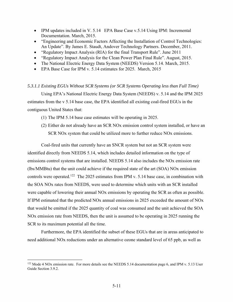
5-11
IPM updates included in V. 5.14 EPA Base Case v.5.14 Using IPM: Incremental Documentation. March, 2015.
“Engineering and Economic Factors Affecting the Installation of Control Technologies: An Update”. By James E. Staudt, Andover Technology Partners. December, 2011.
“Regulatory Impact Analysis (RIA) for the final Transport Rule”. June 2011 “Regulatory Impact Analysis for the Clean Power Plan Final Rule”. August, 2015. The National Electric Energy Data System (NEEDS) Version 5.14. March, 2015. EPA Base Case for IPM v. 5.14 estimates for 2025. March, 2015
5.3.1.1 Existing EGUs Without SCR Systems (or SCR Systems Operating less than Full Time)
Using EPA’s National Electric Energy Data System (NEEDS) v. 5.14 and the IPM 2025
estimates from the v 5.14 base case, the EPA identified all existing coal-fired EGUs in the
contiguous United States that:
(1) The IPM 5.14 base case estimates will be operating in 2025.
(2) Either do not already have an SCR NOx emission control system installed, or have an
SCR NOx system that could be utilized more to further reduce NOx emissions.
Coal-fired units that currently have an SNCR system but not an SCR system were
identified directly from NEEDS 5.14, which includes detailed information on the type of
emissions control systems that are installed. NEEDS 5.14 also includes the NOx emission rate
(lbs/MMBtu) that the unit could achieve if the required state of the art (SOA) NOx emission
controls were operated.122 The 2025 estimates from IPM v. 5.14 base case, in combination with
the SOA NOx rates from NEEDS, were used to determine which units with an SCR installed
were capable of lowering their annual NOx emissions by operating the SCR as often as possible.
If IPM estimated that the predicted NOx annual emissions in 2025 exceeded the amount of NOx
that would be emitted if the 2025 quantity of coal was consumed and the unit achieved the SOA
NOx emission rate from NEEDS, then the unit is assumed to be operating in 2025 running the
SCR to its maximum potential all the time.
Furthermore, the EPA identified the subset of these EGUs that are in areas anticipated to
need additional NOx reductions under an alternative ozone standard level of 65 ppb, as well as
122 Mode 4 NOx emission rate. For more details see the NEEDS 5.14 documentation page 6, and IPM v. 5.13 User Guide Section 3.9.2.

5-12
the smaller subset of the EGUs that are in areas anticipated to need additional NOx reductions
under a 70 ppb ozone standard.
The EPA identified 319 existing coal-fired EGUs nationwide (total capacity 122.4 GW)
that are estimated to continue to be in operation in the 2025 base case that either do not already
have an SCR system (30 units, 5.4 GW) or have an SCR system that is not working full time
(289 units, 117.1 GW) . These 319 EGUs include units both in areas anticipated to need to
reduce NOx emissions (37 units, 8.5 GW) with a 65 ppb ozone NAAQS, as well as the EGUs in
all other areas (282 units, 114.0 MW). All of the 30 EGUs that do not have an SCR are in areas
expected to need to reduce NOx emissions with a 65 ppb NAAQS (30 units, 5.4 GW). The areas
that are expected to need to reduce NOx emissions with a 65 ppb NAAQS also have 7 units (3.1
GW) have an SCR system not working full time.
Upgrading the 30 EGUs to an SCR emission control system will reduce NOx emissions
in areas expected to need additional NOx controls with a 65 ppb NAAQS by a total of 41,400
tons. Operating the 7 EGUs with SCRs system estimated to not be operated as much as possible
in the 65 ppb ozone NAAQS areas an additional 18,300 tons, for a combined total of 59,700 tons
of NOx reduced annually.
Of the 37 EGUs estimated to be able to reduce NOx emissions in the 65 ppb NAAQS
areas, 5 EGUs (1.7 GW) are also in the areas needing additional NOx reductions under a revised
70 ppb ozone NAAQS standard. Installing SCRs on 2 of these units, and running the existing
SCRs as much as possible on the other 3 units, a total of 11,200 tons of NOx in the 70 ppb ozone
NAAQS areas.
Given the nationwide size distribution of the existing EGUs that do not already have an
SCR, or do not operate the existing SCR system full time, we present the illustrative labor
analysis for three different sized “model plants”: 300 MW capacity, 500 MW, and 800 MW.
These three capacity sizes of model plants were selected by examining the distribution of
existing coal-fired EGUs that can either be upgraded to an SCR, or have the existing SCR
operated to as much as possible. Because of the relatively small number (37) of the identified
EGUs in the 65 ppb areas, the distribution of 319 EGUs nationwide better reflects the
distribution of EGUs identified. Figure 5-1 shows the nationwide capacity size distribution of the
319 units. For comparison Figure 5-2 shows the size distribution of the 37 units in the 65 ppb
ozone NAAQS areas. As can be seen in Figure 5-1, the 300 MW capacity “model plant” is the

5-13
most common candidate for installing an SCR system in the 65 ppb areas, but 500 MW and 800
MW units (which are common in the national set of 319 identified units) also exist in the 65 ppb
areas.
Figure 5-1. Size Distribution of Identified 319 Existing Coal-Fired EGU Units Nationwide without SCR NOx Controls (or with SCRs Operated Less Than the Maximum Possible Amount of Time)
Figure 5-2. Size Distribution of 37 Existing Coal-Fired EGU Units without SCR NOx Controls (or with SCRs Operated Less Than the Maximum Possible Amount of Time) in Areas Anticipated to Need Additional NOx Controls With the Alternative 65 ppb Ozone Standard Level
0
10
20
30
40
50
60
70
80
90# of EG
Us
0
5
10
15
20
25
30
35
0 ‐ 400 MW 450 ‐ 650 MW 650 ‐ 1350MW
# of EG
Us
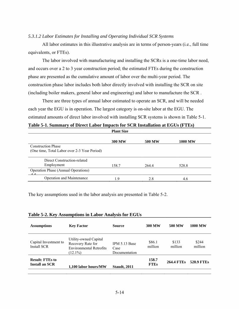
5-14
5.3.1.2 Labor Estimates for Installing and Operating Individual SCR Systems
All labor estimates in this illustrative analysis are in terms of person-years (i.e., full time
equivalents, or FTEs).
The labor involved with manufacturing and installing the SCRs is a one-time labor need,
and occurs over a 2 to 3 year construction period; the estimated FTEs during the construction
phase are presented as the cumulative amount of labor over the multi-year period. The
construction phase labor includes both labor directly involved with installing the SCR on site
(including boiler makers, general labor and engineering) and labor to manufacture the SCR .
There are three types of annual labor estimated to operate an SCR, and will be needed
each year the EGU is in operation. The largest category is on-site labor at the EGU. The
estimated amounts of direct labor involved with installing SCR systems is shown in Table 5-1.
Table 5-1. Summary of Direct Labor Impacts for SCR Installation at EGUs (FTEs) Plant Size
300 MW 500 MW 1000 MW Construction Phase (One time, Total Labor over 2-3 Year Period) Direct Construction-related
Employment 158.7 264.4 528.8 Operation Phase (Annual Operations) 5 5
Operation and Maintenance 1.9 2.8 4.6
The key assumptions used in the labor analysis are presented in Table 5-2.
Table 5-2. Key Assumptions in Labor Analysis for EGUs
Assumptions Key Factor Source 300 MW 500 MW 1000 MW
Capital Investment to Install SCR
Utility-owned Capital Recovery Rate for Environmental Retrofits (12.1%)
IPM 5.13 Base Case Documentation
$86.1 million
$133 million
$244 million
Result: FTEs to Install an SCR
1,100 labor hours/MW Staudt, 2011
158.7 FTEs
264.4 FTEs 528.9 FTEs
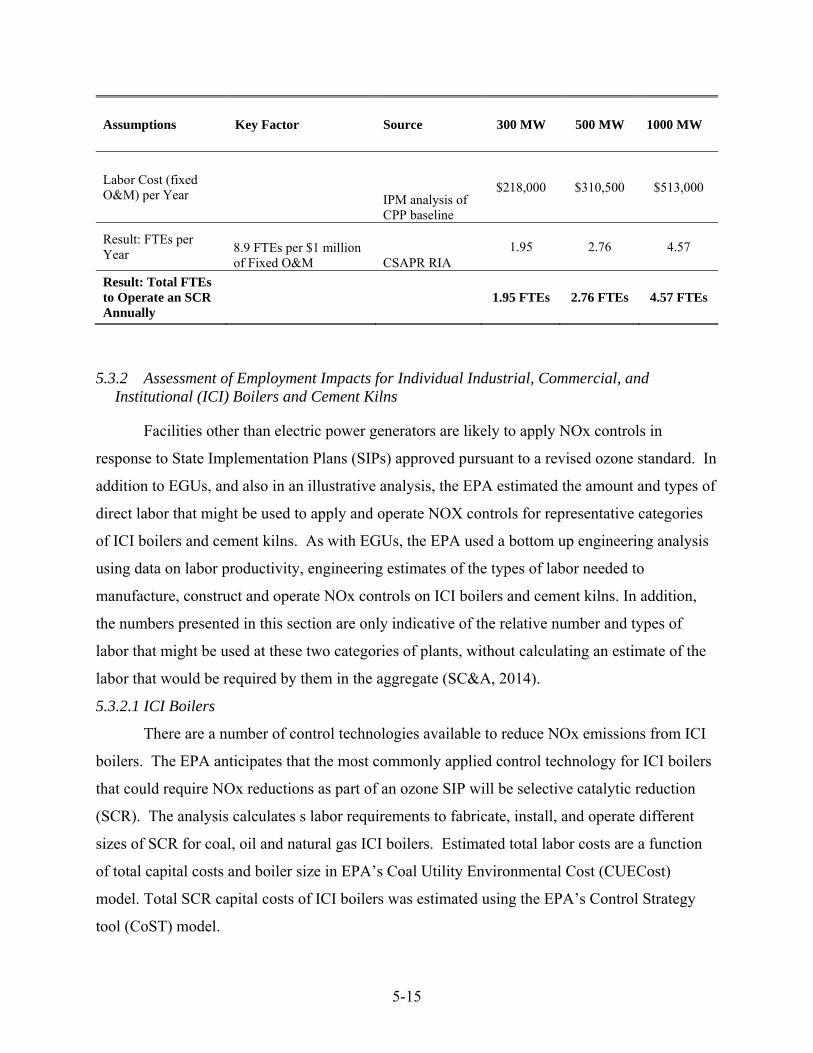
5-15
Assumptions Key Factor Source 300 MW 500 MW 1000 MW
Labor Cost (fixed O&M) per Year
IPM analysis of CPP baseline
$218,000 $310,500 $513,000
Result: FTEs per Year 8.9 FTEs per $1 million
of Fixed O&M CSAPR RIA 1.95 2.76 4.57
Result: Total FTEs to Operate an SCR Annually
1.95 FTEs 2.76 FTEs 4.57 FTEs
5.3.2 Assessment of Employment Impacts for Individual Industrial, Commercial, and Institutional (ICI) Boilers and Cement Kilns
Facilities other than electric power generators are likely to apply NOx controls in
response to State Implementation Plans (SIPs) approved pursuant to a revised ozone standard. In
addition to EGUs, and also in an illustrative analysis, the EPA estimated the amount and types of
direct labor that might be used to apply and operate NOX controls for representative categories
of ICI boilers and cement kilns. As with EGUs, the EPA used a bottom up engineering analysis
using data on labor productivity, engineering estimates of the types of labor needed to
manufacture, construct and operate NOx controls on ICI boilers and cement kilns. In addition,
the numbers presented in this section are only indicative of the relative number and types of
labor that might be used at these two categories of plants, without calculating an estimate of the
labor that would be required by them in the aggregate (SC&A, 2014).
5.3.2.1 ICI Boilers
There are a number of control technologies available to reduce NOx emissions from ICI
boilers. The EPA anticipates that the most commonly applied control technology for ICI boilers
that could require NOx reductions as part of an ozone SIP will be selective catalytic reduction
(SCR). The analysis calculates s labor requirements to fabricate, install, and operate different
sizes of SCR for coal, oil and natural gas ICI boilers. Estimated total labor costs are a function
of total capital costs and boiler size in EPA’s Coal Utility Environmental Cost (CUECost)
model. Total SCR capital costs of ICI boilers was estimated using the EPA’s Control Strategy
tool (CoST) model.

5-16
Just over 24% of total capital costs are for labor used in SCR fabrication. This
percentage was multiplied by the total capital cost, and the resulting dollar amount was
converted into full time equivalents (FTE) based on the average annual salary of workers (as
outlined in IEC, 2011). The annual compensation came from the Bureau of Labor Statistics
(BLS). This salary number was adjusted to account for benefits also based on BLS data. The
total fabrication expenditures were divided by the average fabrication labor compensation to
estimate the number of full time equivalent workers in SCR fabrication (SC&A, 2014).
The calculation of construction or installation labor is based on previous research on
labor required for SCR installation at utility boilers. (Staudt 2011). Based on that, we estimate
that 27% of SCR capital costs are spent on installation labor. We applied that percentage to the
estimates of the capital costs of SCR for ICI boilers to give us the total labor expenditures, which
we then converted to FTE based on average annual compensation provided by BLS.
Operation and Maintenance labor was estimated using the CUECost model
(http://nepis.epa.gov/Adobe/PDF/P1005ODM.pdf). Maintenance and administrative labor for
SCR is estimated to be small in relation to fabrication and construction, with the caveat that
available information on which to base an estimate is sparse. According to the approach used in
the CUECost model, most utility boilers require a full time worker to operate and maintain the
equipment. ICI boilers are much smaller, however.. Table 5-3 below provides summary labor
estimates for SCR at varying sized ICI boilers.
Table 5-3. Summary of Direct Labor Impacts for Individual ICI Boilers
Plant Type Boiler Size (MMBtu/hr)
One-Time Employment Impacts1 (Annual FTEs)
Recurring Annual Employment Impacts2 (FTEs per year)
Coal-fired 750 19.5 1.2 500 15.2 1.1 400 13.6 1.0 250 10.7 0.9 Oil-fired 250 9.8 0.9 150 7.3 0.9 100 5.5 0.8 50 3.2 0.8 Natural Gas-fired 250 10.5 0.9 150 11.0 0.9 100 8.4 0.9 50 6.5 0.8
1. Includes Fabrication and Installation Labor
2. Includes Operations, Maintenance, and Administrative Support

5-17
Similar to the calculations for SCR applied to EGUs, an illustrative analysis based on
engineering costs estimates labor requirements in upstream sectors for SCR applied to
representative ICI boilers. This includes labor requirements in selected major upstream sectors
directly involved in manufacturing the materials used in SCR systems (steel), as well as the
chemicals used to operate an SCR system (ammonia and the catalyst used in the construction and
operation of SCR systems, such as steel, concrete, or chemicals used to manufacture NOx
controls). For an SCR installed at a representative 750 MMBtu/hr coal boiler, we estimate one-
time employment impacts in these related sectors as:of 8.6 FTE, annual recurring impacts of 2.17
FTE for an SCR operated year-round, and annual recurring impacts of 0.90 FTE for an SCR
operated during the five-month ozone season (SC&A, 2014).
5.3.2.2 Cement Kilns
There are a number of technologies that can be used to control NOx emissions at cement
kilns. The analysis focused on synthetic non-catalytic reduction (SNCR) as the most likely
choice for future NOx controls at cement kilns affected by requirements in ozone SIPs.
Although SNCR is not considered an appropriate technology for wet and long dry kilns, most
new or recently constructed kilns will likely be preheater and precalciner kilns, and these kilns
will likely operate using SNCR as a control technology.
The capital costs for equipment supply fabrication were estimated for an SNCR system
for a mid-sized preheater and precalciner kiln (125 to 208 tons of clinker per hour). The percent
of equipment supply fabrication costs of these systems attributable to labor is 44%.
(Wojichowski, 2014). This labor cost was converted to FTE using BLS data. A similar
methodology was used to estimate installation labor. Labor costs for SNCR installation were
estimated by the vendor to be 17% of the total cost. That was converted to FTE using BLS data.
This information is summarized in Table 5-4.
Table 5-4. Estimated Direct Labor Impacts for Individual SNCR Applied to a Mid-Sized Cement Kiln (125-208 tons clinker/hr)
Kiln Type Preheater / Precalciner Equipment Supply Fabrication FTE 1.5 Installation FTE 0.9 O&M Annual Recurring FTE 0.1

5-18
In addition, an illustrative analysis of labor requirements in upstream sectors for SNCR
applied to cement kilns include the labor requirements in selected major upstream sectors
directly involved in manufacturing the materials used in SNCR systems (steel), as well as the
reagent used to operate an SNCR system. For an SNCR installed at a 3,000 tons clinker per day
capacity cement kiln, we estimate employment impacts in these related sectors as one-time
employment impacts of 0.22-0.34 FTE, annual recurring impacts of 0.41 FTE for an SNCR
operated year-round, and annual recurring impacts of 0.28 FTE for an SNCR operated during the
five-month ozone season (SC&A, 2014).
5.4 Conclusion
This chapter presents qualitative and quantitative discussions of potential employment
impacts of the Ozone NAAQS. The qualitative discussion identifies challenges associated with
estimating net employment effects and discusses anticipated impacts related to the rule. It
includes an in-depth discussion of economic theory underlying analysis of employment impacts.
The employment impacts for regulated firms can be decomposed into output and substitution
effects, both of which may be positive or negative. Consequently, economic theory alone cannot
predict the direction or magnitude of a regulation’s employment impact. It is possible to combine
theory with empirical studies specific to the regulated firms and other relevant sectors if data and
methods of sufficient detail and quality are available. Finally, economic theory suggests that
environmental regulations may have positive impacts on labor supply and productivity as well.
We examine the peer-reviewed economics literature analyzing various aspects of labor
demand, relying on the above theoretical framework. Determining the direction of employment
effects in regulated industries is challenging because of the complexity of the output and
substitution effects. Complying with a new or more stringent regulation may require additional
inputs, including labor, and may alter the relative proportions of labor and capital used by
regulated firms (and firms in other relevant industries) in their production processes. The
available literature illustrates some of the difficulties for empirical estimation. Econometric
studies of environmental rules converge on the finding that employment effects, whether positive
or negative, have been small in regulated sectors.

5-19
The illustrative quantitative analysis in this chapter projects a subset of potential
employment impacts in the electricity generation sector and for ICI boilers and cement kilns.
States have the responsibility and flexibility to implement plans to meet the Ozone NAAQS. As
such, given the wide range of approaches that may be used, quantifying the associated
employment impacts is difficult. This analysis presents employment impact estimates based on
used a bottom up engineering analysis using data on labor productivity, engineering estimates of
the types of labor needed to manufacture, construct and operate NOx controls for EGUs, ICI
boilers and cement kilns.
5.5 References
Arrow, K. J.; M. L. Cropper; G. C. Eads; R. W. Hahn; L. B. Lave; R. G. Noll; Paul R. Portney; M. Russell; R. Schmalensee; V. K. Smith and R. N. Stavins. 1996. “Benefit-Cost Analysis in Environmental, Health, and Safety Regulation: A Statement of Principles.” American Enterprise Institute, the Annapolis Center, and Resources for the Future; AEI Press. Available at <http://www.hks.harvard.edu/fs/rstavins/Papers/Benefit Cost Analysis in Environmental.AEI.1996.pdf>. Accessed June 5, 2015.
Berman, E. and L. T. M. Bui. 2001. “Environmental Regulation and Labor Demand: Evidence from the South Coast Air Basin.” Journal of Public Economics. 79(2): 265-295.
Bureau of Labor Statistics, 2011. “National Compensation Survey: Occupational Earnings in the United States, 2010.” Located online at: http://www.bls.gov/ncs/ncswage2010.htm#Wage_Tables
Bureau of Labor Statistics, 2014. “Employer Costs for Employee Compensation”. Released September 10, 2014. Located online at: http://www.bls.gov/news.release/ecec.toc.htm
Congressional Budget Office (2011), Statement of Douglas W. Elmendorf, Director, before the Senate Budget Committee, “Policies for Increasing Economic Growth and Employment in 2012 and 2013” (November 15)<http://www.cbo.gov/sites/default/files/11-15-Outlook_Stimulus_Testimony.pdf>
Ehrenberg, R. G. and R. S. Smith. 2000. Modern Labor Economics: Theory and Public Policy. Addison Wesley Longman, Inc., Chapter 4.
Executive Order 13563 (January 21, 2011). “Improving Regulation and Regulatory Review. Section 1. General Principles of Regulation.” Federal Register 76(14): 3821-3823.
Ferris, A. E., R. J. Shadbegian, A. Wolverton. 2014. “The Effect of Environmental Regulation on Power Sector Employment: Phase I of the Title IV SO2 Trading Program.” Journal of the Association of Environmental and Resource Economists. 1(4): 521-553.
Greenstone, M. 2002. “The Impacts of Environmental Regulations on Industrial Activity: Evidence from the 1970 and 1977 Clean Air Act Amendments and the Census of Manufactures.” Journal of Political Economy. 110(6): 1175-1219.
Hamermesh, D. S. 1993. Labor Demand. Princeton, NJ: Princeton University Press. Chapter 2.
Kahn, M.E. and E. T. Mansur. 2013. “Do Local Energy Prices and Regulation Affect the Geographic Concentration of Employment?” Journal of Public Economics. 101:105–114.

5-20
Layard, P.R.G. and A. A. Walters. 1978. Microeconomic Theory. McGraw-Hill, Inc. Chapter 9.
List, J. A.; D. L. Millimet; P. G. Fredriksson and W. W. McHone. 2003. “Effects of Environmental Regulations on Manufacturing Plant Births: Evidence from a Propensity Score Matching Estimator.” The Review of Economics and Statistics. 85(4): 944-952.
Marshall, A. 1920. Principles of Economics. Library of Economics and Liberty. Available at: <http://www.econlib.org/library/Marshall/marP.html> .
SC&A,2014:, Assessment of Employment Impacts of NOx Controls. Memorandum prepared to Jason Price, IEc and Ellen Kurlansky, US EPA., prepared by J. Wilson; M Mullen; and j Schreiber, SC&A, Inc. September 2014
Schmalansee, R. and R. Stavins (2011). “A Guide to Economic and Policy Analysis for the Transport Rule.” White Paper. Boston, MA. Exelon Corp.
Smith, K. 2012. “Reflections: In Search of Crosswalks between Macroeconomics and Environmental Economics.” Review of Environmental Economics and Policy. 6(2):298-317.
Staudt, 2011: Staudt, James E., Engineering and Economic Factors Affecting the Installation of Control Technologies—An Update, Andover Technology Partners, North Andover, MA, December 15, 2011.
U.S. Environmental Protection Agency (U.S. EPA), 2002: USEPA Office of Air Quality Planning and Standards, EPA Air Pollution Control Cost Manual, Sixth Edition, EPA/452/B-02-001, Research Triangle Park, NC, January 2002.
U.S. Environmental Protection Agency (U.S. EPA), 2007: Alternative Control Techniques Document Update – NOx Emissions from New Cement Kilns, EPA-453/R-07-006, prepared by EPA and Research Triangle Institute for EPA Office of Air Quality Planning and Standards, Sector Policies and Programs Division, November 2007.
U.S. Environmental Protection Agency (U.S. EPA). 2011. Regulatory Impact Assessment for the Cross State Air Pollution Rule. Office of Air Quality Planning and Standards, Research Triangle Park, NC. Available at http://www.epa.gov/airtransport/pdfs/FinalRIA.pdf.
U.S. Environmental Protection Agency (U.S. EPA). 2015. Regulatory Impact Analysis for the Clean Power Plan Final Rule. Office of Air and Radiation, Washington, D.C. Available at: http://www.epa.gov/airquality/cpp/cpp-final-rule-ria.pdf.
Wojichowski, 2014: David Wojichowski, De-Nox Technologies, LLC, SNCR cost estimates provided to Maureen Mullen, SC&A via email, September 25, 2014.

6-1
CHAPTER 6: HUMAN HEALTH BENEFITS ANALYSIS APPROACH AND RESULTS
6.1 Summary
This chapter of the Regulatory Impact Analysis (RIA) presents the estimated human
health benefits for the revised National Ambient Air Quality Standards (NAAQS) for ozone. In
this chapter, we quantify the health-related benefits of the ozone air quality improvements
resulting from the illustrative emissions control strategies that reduce emissions of the ozone
precursor pollutants (i.e., nitrogen oxides (NOx) and volatile organic compounds (VOCs)) to
reach the revised and alternative ozone NAAQS standard levels. We also estimate the health co-
benefits of the fine particulate matter (PM2.5)-related air quality improvements that would occur
as a result of reducing NOx emissions.123
We selected 2025 as the primary year of analysis because the Clean Air Act requires
most areas of the U.S. to meet a revised ozone standard by 2025. The benefits of each standard
alternative are estimated as being incremental to attaining the existing standard of 75 ppb.124
These estimated benefits are incremental to the benefits estimated for several recent rules (e.g.,
U.S. EPA, 2011c and U.S. EPA, 2014a). We estimated the benefits of California attaining a
revised standard in 2038 to account for the fact that many locations in this state must attain a
revised standard later than the rest of the U.S. In this chapter, we refer to estimates of nationwide
benefits of attaining an alternative standard everywhere in the U.S. except California as the 2025
scenario. The post-2025 scenario refers to estimates of nationwide benefits of attaining an
alternative standard just in California. Because we estimate incremental costs and benefits for
these two distinct scenarios reflecting attainment in different years it is not appropriate to either
sum, or directly compare, the estimates.
Table 6-1 summarizes the estimated monetized benefits (total and ozone only) of
attaining the revised and alternative ozone standards of 70 ppb and 65 ppb, respectively, in 2025.
Table 6-2 presents the same types of benefit estimates for the scenario. These estimates reflect
the sum of the economic value of estimated morbidity and mortality effects related to changes in
exposure to ozone and PM2.5. Although these tables present ozone and PM2.5-related benefits
123 VOC reductions associated with simulated attainment of the revised and alternative ozone standards also have the
potential to impact PM2.5 concentrations, but we were not able to estimate those effects. 124 The current standard is the 4th highest daily maximum 8-hour ozone concentration of 75 ppb.
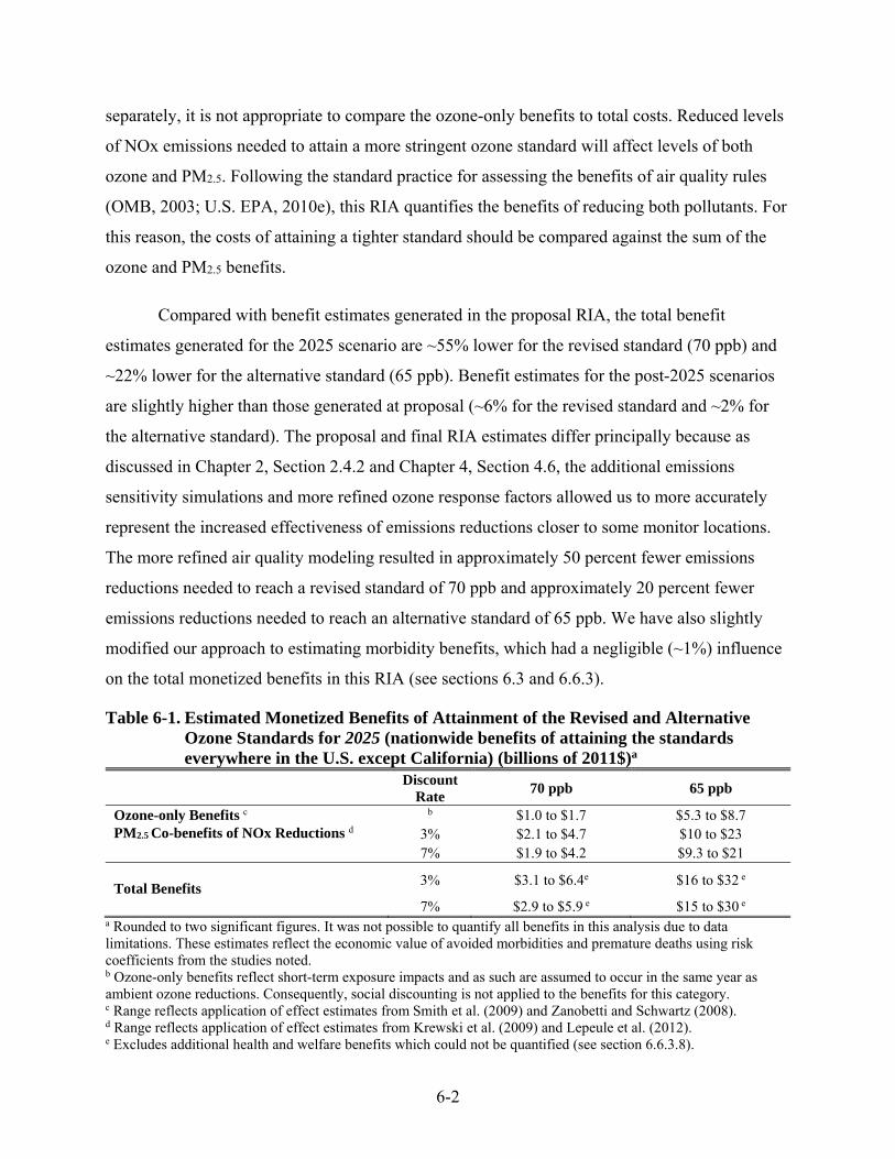
6-2
separately, it is not appropriate to compare the ozone-only benefits to total costs. Reduced levels
of NOx emissions needed to attain a more stringent ozone standard will affect levels of both
ozone and PM2.5. Following the standard practice for assessing the benefits of air quality rules
(OMB, 2003; U.S. EPA, 2010e), this RIA quantifies the benefits of reducing both pollutants. For
this reason, the costs of attaining a tighter standard should be compared against the sum of the
ozone and PM2.5 benefits.
Compared with benefit estimates generated in the proposal RIA, the total benefit
estimates generated for the 2025 scenario are ~55% lower for the revised standard (70 ppb) and
~22% lower for the alternative standard (65 ppb). Benefit estimates for the post-2025 scenarios
are slightly higher than those generated at proposal (~6% for the revised standard and ~2% for
the alternative standard). The proposal and final RIA estimates differ principally because as
discussed in Chapter 2, Section 2.4.2 and Chapter 4, Section 4.6, the additional emissions
sensitivity simulations and more refined ozone response factors allowed us to more accurately
represent the increased effectiveness of emissions reductions closer to some monitor locations.
The more refined air quality modeling resulted in approximately 50 percent fewer emissions
reductions needed to reach a revised standard of 70 ppb and approximately 20 percent fewer
emissions reductions needed to reach an alternative standard of 65 ppb. We have also slightly
modified our approach to estimating morbidity benefits, which had a negligible (~1%) influence
on the total monetized benefits in this RIA (see sections 6.3 and 6.6.3).
Table 6-1. Estimated Monetized Benefits of Attainment of the Revised and Alternative Ozone Standards for 2025 (nationwide benefits of attaining the standards everywhere in the U.S. except California) (billions of 2011$)a
Discount
Rate 70 ppb 65 ppb
Ozone-only Benefits c b $1.0 to $1.7 $5.3 to $8.7 PM2.5 Co-benefits of NOx Reductions d 3% $2.1 to $4.7 $10 to $23
7% $1.9 to $4.2 $9.3 to $21 Total Benefits
3% $3.1 to $6.4e $16 to $32 e
7% $2.9 to $5.9 e $15 to $30 e a Rounded to two significant figures. It was not possible to quantify all benefits in this analysis due to data limitations. These estimates reflect the economic value of avoided morbidities and premature deaths using risk coefficients from the studies noted. b Ozone-only benefits reflect short-term exposure impacts and as such are assumed to occur in the same year as ambient ozone reductions. Consequently, social discounting is not applied to the benefits for this category. c Range reflects application of effect estimates from Smith et al. (2009) and Zanobetti and Schwartz (2008). d Range reflects application of effect estimates from Krewski et al. (2009) and Lepeule et al. (2012). e Excludes additional health and welfare benefits which could not be quantified (see section 6.6.3.8).

6-3
Table 6-2. Estimated Monetized Benefits of Attainment of the Revised and Alternative
Ozone Standards for post-2025 (nationwide benefits of attaining the standards just in California) (billions of 2011$)a
Discount
Rate 70 ppb 65 ppb
Ozone-only Benefits c b $0.79 to $1.3 $1.6 to $2.6 PM2.5 Co-benefits of NOx reductions d 3% $0.40 to $0.91 $0.79 to $1.8
7% $0.37 to $0.82 $0.71 to $1.6
Total Benefits
3% $1.2 to $2.2 e $2.4 to $4.4 e
7% $1.2 to $2.1 e $2.3 to $4.2 e a Rounded to two significant figures. It was not possible to quantify all benefits in this analysis due to data limitations. These estimates reflect the economic value of avoided morbidities and premature mortalities using risk coefficients from the studies noted. b Ozone-only benefits reflect short-term exposure impacts and as such are assumed to occur in the same year as ambient ozone reductions. Consequently, social discounting is not applied to the benefits for this category. c Range reflects application of effect estimates from Smith et al. (2009) and Zanobetti and Schwartz (2008). d Range reflects application of effect estimates from Krewski et al. (2009) and Lepeule et al. (2012). e Excludes additional health and welfare benefits which could not be quantified (see section 6.6.3.8).
The control measures (identified and unidentified) applied to reach the revised and
alternative ozone standards would reduce other ambient pollutants, including VOCs and NO2.
However, because the method used in this analysis to simulate attainment does not account for
changes in ambient concentrations of other pollutants, we were unable to quantify the co-benefits
of reduced exposure to these pollutants. Due to limited data and methods, we were unable to
estimate some anticipated health benefits associated with exposure to ozone and PM2.5.
6.2 Overview
This chapter presents estimated health benefits for the revised and alternative ozone
standards (70 ppb and 65 ppb, respectively) that the EPA could quantify, given the available
resources, data and methods. This chapter characterizes the benefits of the application of the
identified and unidentified control strategies identified in Chapter 3 for the revised and
alternative ozone standards by answering three key questions:
1. What health effects are estimated to be avoided by reducing ambient ozone levels to attain the revised and alternative ozone standards?
2. What is the estimated economic value of these effects?

6-4
3. What are the co-benefits of reductions in ambient PM2.5 associated with reductions in emissions of ozone precursors (specifically NOx)?
In this analysis, we quantify an array of adverse health impacts associated with to ozone
and PM2.5 that would be avoided by attaining a revised ozone standard. The Integrated Science
Assessment for Ozone and Related Photochemical Oxidants (“ozone ISA”) (U.S. EPA, 2013a)
identifies the human health effects associated with ozone exposure, which include premature
mortality and a variety of illnesses associated with acute (days-long) and chronic (months to
years-long) exposures. Similarly, the Integrated Science Assessment for Particulate Matter (“PM
ISA”) (U.S. EPA, 2009b) identifies the human health effects associated with ambient particles,
which include premature mortality and a variety of illnesses associated with acute and chronic
exposures. Air pollution can affect human health in a variety of ways. In Table 6-3 we
summarize the “categories” of effects and describe those that we quantified for this analysis and
those we were unable to quantify due to lack of resources, data, or methods.
This list of benefit categories is not exhaustive, and we are not always able to quantify
each effect completely. In this RIA, we only quantify endpoints that are classified in the ozone
and PM ISAs as being causally related, or likely to be causally related, to each pollutant.
Following this criterion, we excluded some effects that were identified in previous lists of
unquantified benefits in other RIAs (e.g., UVb exposure), but are not identified in the most
recent ISA as having a causal or likely causal relationship with ozone. This way of selecting
endpoints for quantification should not be interpreted as a change in the level of evidence
regarding the association between these endpoints and ozone (or PM2.5) exposure.
This benefits analysis relies on an array of data inputs—including emissions estimates,
modeled ozone concentrations, health impact functions and valuation estimates among others—
which are themselves subject to uncertainty and may in turn contribute to the overall uncertainty
in this analysis. We employ several techniques to characterize this uncertainty, which are
described in detail in sections 6.5 and 6.7.3.
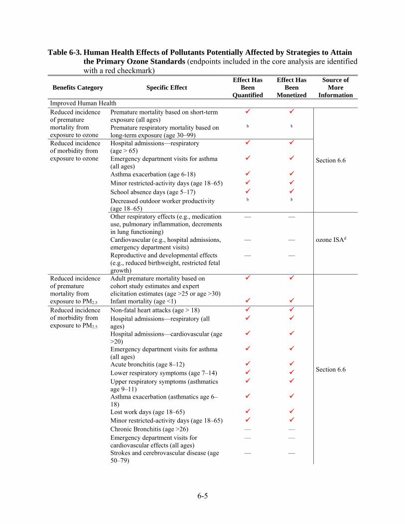
6-5
Table 6-3. Human Health Effects of Pollutants Potentially Affected by Strategies to Attain the Primary Ozone Standards (endpoints included in the core analysis are identified with a red checkmark)
Benefits Category Specific Effect Effect Has
Been Quantified
Effect Has Been
Monetized
Source of More
Information Improved Human Health Reduced incidence of premature mortality from exposure to ozone
Premature mortality based on short-term exposure (all ages)
Section 6.6
Premature respiratory mortality based on long-term exposure (age 30–99)
b b
Reduced incidence of morbidity from exposure to ozone
Hospital admissions—respiratory (age > 65)
Emergency department visits for asthma (all ages)
Asthma exacerbation (age 6-18) Minor restricted-activity days (age 18–65) School absence days (age 5–17) Decreased outdoor worker productivity (age 18–65)
b b
Other respiratory effects (e.g., medication use, pulmonary inflammation, decrements in lung functioning)
— —
ozone ISAd
Cardiovascular (e.g., hospital admissions, emergency department visits)
— —
Reproductive and developmental effects (e.g., reduced birthweight, restricted fetal growth)
— —
Reduced incidence of premature mortality from exposure to PM2.5
Adult premature mortality based on cohort study estimates and expert elicitation estimates (age >25 or age >30)
Section 6.6
Infant mortality (age <1) Reduced incidence of morbidity from exposure to PM2.5
Non-fatal heart attacks (age > 18) Hospital admissions—respiratory (all ages)
Hospital admissions—cardiovascular (age >20)
Emergency department visits for asthma (all ages)
Acute bronchitis (age 8–12) Lower respiratory symptoms (age 7–14) Upper respiratory symptoms (asthmatics age 9–11)
Asthma exacerbation (asthmatics age 6–18)
Lost work days (age 18–65) Minor restricted-activity days (age 18–65) Chronic Bronchitis (age >26) — — Emergency department visits for cardiovascular effects (all ages)
— —
Strokes and cerebrovascular disease (age 50–79)
— —

6-6
Benefits Category Specific Effect Effect Has
Been Quantified
Effect Has Been
Monetized
Source of More
Information Other cardiovascular effects (e.g., other ages)
— —
PM ISAc Other respiratory effects (e.g., pulmonary function, non-asthma ER visits, non-bronchitis chronic diseases, other ages and populations)
— —
Reproductive and developmental effects (e.g., low birth weight, pre-term births, etc.)
— —
PM ISA c,d Cancer, mutagenicity, and genotoxicity effects
— —
Reduced incidence of morbidity from exposure to NO2
Asthma hospital admissions (all ages) — —
NO2 ISA e
Chronic lung disease hospital admissions (age > 65)
— —
Respiratory emergency department visits (all ages)
— —
Asthma exacerbation (asthmatics age 4–18)
— —
Acute respiratory symptoms (age 7–14) — — Premature mortality — —
NO2 ISA c,d Other respiratory effects (e.g., airway hyperresponsiveness and inflammation, lung function, other ages and populations)
— —
b We quantified these benefits, but they are not part of the core monetized benefits. c We assess these benefits qualitatively because we do not have sufficient confidence in available data or methods. d We assess these benefits qualitatively because current evidence is only suggestive of causality or there are other significant concerns over the strength of the association. e We assess these benefits qualitatively due to time and resource limitations for this analysis.
The remainder of this chapter is organized as follows: Section 6.3 includes a discussion
of the methodological updates represented in this analysis; Section 6.4 includes a discussion of
the methodologies used in the human health benefits analyses; Section 6.5 includes a
characterization of uncertainty; Section 6.6 details the data inputs used in the analysis, including
demographic data, baseline incidence and prevalence estimates, effect coefficients, and
economic valuation estimates; Section 6.7 presents the results; and Section 6.8 includes a brief
discussion of the results. In addition, the chapter has several appendices that provide more
details on the following: Appendix 6A includes a detailed characterization of uncertainty in the
analysis; Appendix 6B includes additional quantitative analyses supporting uncertainty
characterization.

6-7
6.3 Updated Methodology Presented in the Proposal and Final RIAs
Both the proposed and final RIAs for this ozone standard incorporate an array of policy
and technical updates to the benefits analysis methods since the previous review the ozone
standards in 2008 and the proposed reconsideration in 2010.
1. To be consistent with Agency guidance, EPA revised the Value of Statistical Life (VSL) it used to quantify the value of reduced mortality risk (see the NO2 NAAQS final RIA (U.S. EPA, 2010a) for further discussion).
2. The population demographic data in BenMAP-CE (U.S. EPA, 2015a) reflects the 2010 Census and future projections based on economic forecasting models developed by Woods and Poole, Inc. (Woods and Poole, 2012). These data replace older demographic projection data from Woods and Poole (2007). This update was introduced in the final PM NAAQS RIA (U.S. EPA, 2012a).
3. The baseline incidence rates used to quantify air pollution-related hospital admissions and emergency department visits and the asthma prevalence rates were updated to replace the earlier rates. This update was introduced in the final CSAPR (U.S. EPA, 2011c).
4. The cost-of-illness estimates for hospital admissions, including median wages, have been updated to reflect 2007 data. This update was introduced in the proposal PM NAAQS RIA (U.S. EPA, 2012a).
5. Updates specific to estimating ozone-related effects:
a. New studies used to quantify ozone-related premature mortality.
i. The ozone ISA (U.S. EPA, 2013a) identifies several new epidemiological studies examining the association between ozone exposure and premature mortality. We include two new multi-city studies to estimate premature mortality attributable to short-term exposure (Smith et al., 2009 and Zanobetti and Schwartz 2008). We also estimate long-term respiratory premature mortality using Jerrett et al. (2009).125 We introduced this update in the proposal RIA (U.S. EPA, 2014c).
ii. Following completion of the proposal RIA (U.S. EPA, 2014c), we slightly modified the methods applied in this RIA. As described in sections 6.6.3, we modified the set of epidemiology studies and associated effect coefficients used in estimating changes in asthma exacerbation and respiratory hospital admissions associated with ozone exposure. Because these changes do not involve our approach for estimating air pollution-related premature mortality,
125 Because we do not have information on the cessation lag for premature mortality from long-term ozone exposure, we do not include the monetized benefits in the core analysis. Instead, monetized benefits associated with long-term ozone-related respiratory mortality are included as a sensitivity analysis (see Appendix 6B, section 6B.2).

6-8
which largely drives overall monetized benefits, they have a negligible (~1%) impact on total monetized benefits (see section 6.6.3 for further discussion).
b. New studies used to quantify ozone-related morbidity effects. The ozone ISA (U.S.
EPA, 2013a) identifies several new epidemiological studies examining the association between short-term ozone exposure and respiratory hospitalizations, respiratory emergency department visits, and exacerbated asthma. We introduced this update in the proposal RIA (U.S. EPA, 2014c).
c. Expanded uncertainty assessment. We added a comprehensive, qualitative assessment of the various uncertain parameters and assumptions within the benefits analysis and expanded the evaluation of air quality benchmarks for ozone-related mortality. We introduced this expanded assessment in the proposal RIA (U.S. EPA, 2014c).
6. Updates specific to estimating PM2.5-related effects:
d. When estimating PM2.5-related health effects, EPA no longer assumed a minimum concentration at which no effects occurred, while still reporting a range of sensitivity estimates based on the EPA’s PM2.5 mortality expert elicitation (see the Portland Cement NESHAP proposal RIA (U.S. EPA, 2009a) for further discussion).
e. New studies used to quantify PM2.5-related premature mortality. We updated the
American Cancer Society cohort study to Krewski et al. (2009) and updated the Harvard Six Cities cohort study to Lepeule et al. (2012). The update for the American Cancer Society cohort was introduced in the proposal RIA for the PM NAAQS review (U.S. EPA, 2012a) and the update for the Harvard Six Cities cohort was introduced in the final RIA for the PM NAAQS review (U.S. EPA, 2012c).
f. New studies used to quantify PM2.5 morbidity. Based on the PM ISA and PM Provisional Assessment, we added several new studies and morbidity endpoints to our health impact assessment, including hospital admissions and emergency department visits. These updates were introduced in the proposal (U.S. EPA, 2012a) and final RIAs for the PM NAAQS review (U.S. EPA, 2012c).
g. More recent survival rates for non-fatal acute myocardial infarctions. Based on recent data from Agency for Healthcare Research and Quality’s Healthcare Utilization Project National Inpatient Sample database (AHRQ, 2009), we identified premature mortality rates for adults hospitalized with acute myocardial infarction stratified by age. These rates replaced the survival rates from Rosamond et al. (1999). This update was introduced in the final RIA for the PM NAAQS review (U.S. EPA, 2012c).
h. Expanded uncertainty assessment. We expanded the comprehensive assessment of the various uncertain parameters and assumptions within the benefits analysis including the evaluation of air quality benchmarks. This update was introduced in the proposed CSAPR RIA (U.S. EPA, 2010f) and refined in the final PM NAAQS RIA (U.S. EPA, 2012c).
6-9
6.4 Human Health Benefits Analysis Methods
We follow a “damage-function” approach in calculating total benefits of the modeled
changes in environmental quality. This approach estimates changes in individual health
endpoints (i.e., specific effects that can be associated with changes in air quality) and assigns
values to those changes assuming independence of the values for those individual endpoints.
Total benefits are calculated simply as the sum of the values for all non-overlapping health
endpoints. The “damage-function” approach is the standard method that EPA uses for assessing
costs and benefits of environmental quality policies and has been used in several recent analyses
published in the peer reviewed scientific literature as well (Levy et al., 2009; Fann et al., 2012a;
Tagaris et al., 2009).
To assess economic values in a damage-function framework, the changes in
environmental quality must be translated into effects on people or on the things that people
value. In some cases, the changes in environmental quality can be valued directly, as is the case
for changes in visibility. In other cases, such as for changes in health outcomes associated with
reductions in ozone and PM concentrations, an impact analysis must first be conducted to
convert air quality changes into effects that can be assigned dollar values. For the purposes of
this RIA, the health impacts analysis (HIA) is limited to those health effects that the ISA
identified as causally or likely causally linked to ambient levels of ozone and PM2.5.
We note at the outset that the EPA rarely has the time or resources to perform extensive
new research to measure directly either the health outcomes or their values for regulatory
analyses. Thus, similar to Kunzli et al. (2000) and other, more recent health impact analyses, our
estimates are based on the best available methods of benefits transfer. Benefits transfer is the
science and art of adapting primary research from similar contexts to obtain the most accurate
measure of benefits for the environmental quality change being analyzed. Adjustments are made
for the level of environmental quality change, the socio-demographic and economic
characteristics of the affected population, and other factors to improve the accuracy and
robustness of benefits estimates.
6-10
Benefits estimates for ozone were generated using the damage function approach outlined
above wherein potential changes in ambient ozone levels (associated with future attainment of
the revised and alternative standard levels) were explicitly modeled and then translated into
reductions in the incidence of specific health endpoints (see Chapter 2 for more information). In
contrast, in estimating PM2.5 co-benefits we utilized a reduced form approach. The details of both
approaches are described in additional detail below.
6.4.1 Health Impact Assessment
The health impact assessment (HIA) quantifies the changes in the incidence of adverse
health impacts resulting from changes in human exposure to PM2.5 and ozone air quality. HIAs
are a well-established approach for estimating the retrospective or prospective change in adverse
health impacts expected to result from population-level changes in exposure to pollutants (Levy
et al., 2009). PC-based tools such as the environmental Benefits Mapping and Analysis Program
– Community Edition (BenMAP-CE) can systematize health impact analyses by applying a
database of key input parameters, including health impact functions and population projections—
provided that key input data are available, including air quality estimates and risk coefficients
(U.S. EPA, 2015a). Analysts have applied the HIA approach to estimate human health impacts
resulting from hypothetical changes in pollutant levels (Hubbell et al., 2005; Tagaris et al., 2009;
Fann et al., 2012a). The EPA and others have relied upon this method to predict future changes
in health impacts expected to result from the implementation of regulations affecting air quality
(e.g., U.S. EPA, 2014a). For this assessment, the HIA is limited to those health effects that are
directly linked to ambient ozone and PM2.5 concentrations. There may be other indirect health
impacts associated with applying emissions controls, such as occupational health exposures.
The HIA approach used in this analysis involves three basic steps: (1) using projections
of ozone air quality126 and estimating the change in the spatial distribution of the ambient air
quality; (2) determining the subsequent change in population-level exposure; and (3) calculating
health impacts by applying concentration-response (C-R) relationships drawn from the
epidemiological literature to this change in population exposure (Hubbell et al., 2009).

6-11
A typical health impact function might look as follows:
∆ 1 ∙∆ ∙ (6.1)
where y0 is the baseline incidence rate for the health endpoint being quantified (for
example, a health impact function quantifying changes in mortality would use the baseline, or
background, mortality rate for the given population of interest); Pop is the population affected by
the change in air quality; x is the change in air quality; and β is the effect coefficient drawn
from the epidemiological study. Figure 6-1 provides a simplified overview of this approach.
Additional detail on the specific types of C-R functions (utilizing epidemiology-based effect
estimates) involved in benefits modeling can be found in the Appendix C of the User’s Manual
Appendices supporting BenMAP-CE (U.S. EPA, 2015b). Specific effect estimates used in this
RIA are documented in section 6.6.3.
Figure 6-1. Illustration of BenMAP-CE Approach
Baseline Air Quality Post‐Policy Scenario Air Quality
Incremental Air Quality
Improvement
Ozone Reduction
PopulationAges 30 ‐99
BackgroundIncidence
RateEffect
Estimate
Mortality Reduction
6-12
6.4.2 Economic Valuation of Health Impacts
After quantifying the change in adverse health impacts, the final step is to estimate the
economic value of these avoided impacts. The appropriate economic value for a change in a
health effect depends on whether the health effect is viewed ex ante (before the effect has
occurred) or ex post (after the effect has occurred). Reductions in ambient concentrations of air
pollution generally lower the risk of future adverse health effects by a small amount for a large
population. The appropriate economic measure is therefore ex ante willingness to pay (WTP) for
changes in risk. Epidemiological studies generally provide estimates of the changes in risk for a
particular health effect for a given increment of air pollution (often per 10 ppb ozone). These
relative risks can be used to develop risk coefficients that relate a unit reduction in ozone or
PM2.5 to changes in the incidence of a health effect. In order to value these changes in incidence,
WTP for changes in risk need to be converted into WTP per statistical incidence. This measure is
calculated by dividing individual WTP for a risk reduction by the related observed change in
risk. For some health effects, such as hospital admissions, WTP estimates are generally not
available. In these cases, we use the costs of treating or mitigating the effect, which generally
understate the true value of reductions in risk of a health effect because they exclude the value of
avoided pain and suffering from the health effect.
We use the BenMAP-CE version 1.1 (U.S. EPA, 2015a, 2015b) to estimate the health
impacts and monetized health benefits for the standards evaluated here. The environmental
Benefits Mapping and Analysis Program—Community Edition (BenMAP-CE) is an open-source
PC-based tool that quantifies the number and economic value of air pollution-related deaths and
illnesses.127 Figure 6-2 shows the data inputs and outputs for the BenMAP-CE program.
127 As compared to the version that it replaces (BenMAP v4), BenMAP-CE uses the same computational algorithms
and input data to calculate benefits for a given air quality change, both versions report the same estimates, within rounding. BenMAP-CE differs from the legacy version of BenMAP in two important ways: (1) it is open-source and the uncompiled code is available to the public; and (2) it is written in C#, which is both more broadly used and modern than the code it replaces (Delphi). BenMAP-CE was last used to support the Health Risk and Exposure Assessment for Ozone (ozone HREA) (U.S. EPA, 2014b).
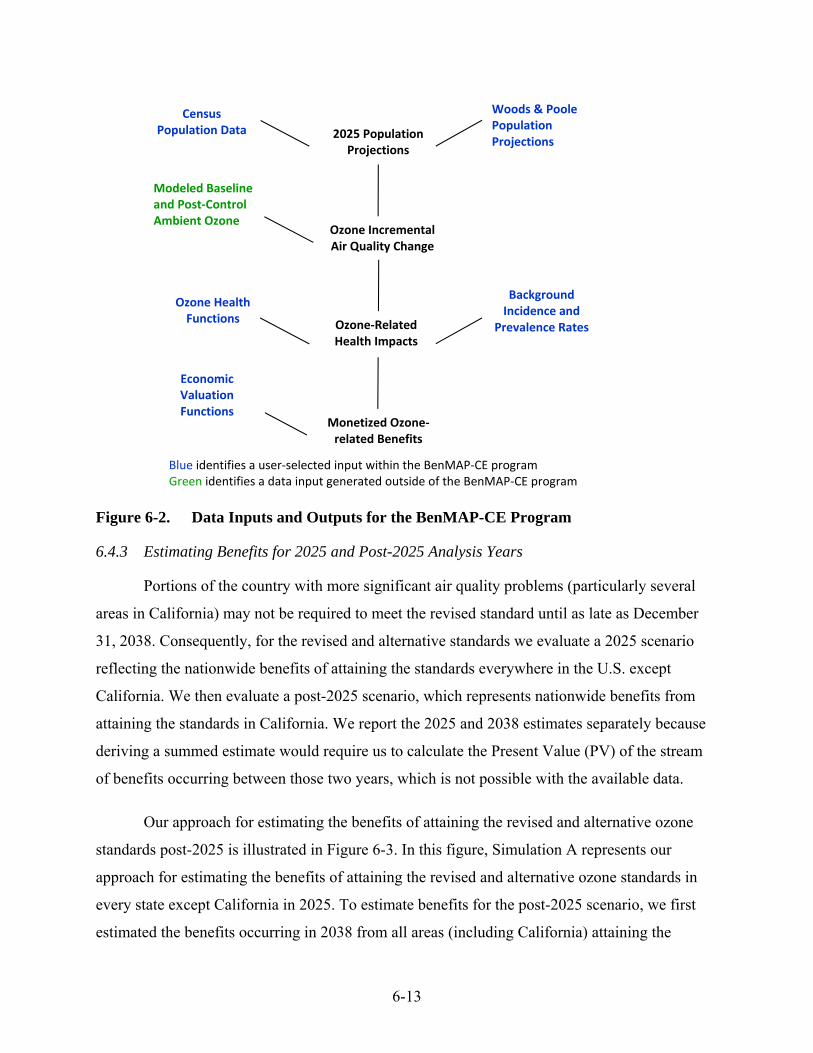
6-13
Figure 6-2. Data Inputs and Outputs for the BenMAP-CE Program
6.4.3 Estimating Benefits for 2025 and Post-2025 Analysis Years
Portions of the country with more significant air quality problems (particularly several
areas in California) may not be required to meet the revised standard until as late as December
31, 2038. Consequently, for the revised and alternative standards we evaluate a 2025 scenario
reflecting the nationwide benefits of attaining the standards everywhere in the U.S. except
California. We then evaluate a post-2025 scenario, which represents nationwide benefits from
attaining the standards in California. We report the 2025 and 2038 estimates separately because
deriving a summed estimate would require us to calculate the Present Value (PV) of the stream
of benefits occurring between those two years, which is not possible with the available data.
Our approach for estimating the benefits of attaining the revised and alternative ozone
standards post-2025 is illustrated in Figure 6-3. In this figure, Simulation A represents our
approach for estimating the benefits of attaining the revised and alternative ozone standards in
every state except California in 2025. To estimate benefits for the post-2025 scenario, we first
estimated the benefits occurring in 2038 from all areas (including California) attaining the
Modeled Baseline and Post‐Control Ambient Ozone
Ozone Health Functions
Economic Valuation Functions
2025 Population Projections
Ozone Incremental Air Quality Change
Ozone‐Related Health Impacts
Woods & Poole Population Projections
Background Incidence and
Prevalence Rates
Monetized Ozone‐related Benefits
Blue identifies a user‐selected input within the BenMAP‐CE programGreen identifies a data input generated outside of the BenMAP‐CE program
Census Population Data

6-14
revised and alternative standards (Simulation C). Next, we simulated the nationwide benefits of
attaining the revised and alternative ozone standards in 2038 for every state except California
(Simulation B). We then subtracted Simulation B from Simulation C to calculate the benefits of
attaining the revised and alternative ozone standards after 2025— that is, to calculate the
nationwide benefits from California alone attaining the standards in 2038. Important caveats are
associated with this approach mentioned in Section 6.1 and discussed further in section 6.7.3.
Figure 6-3. Procedure for Generating Benefits Estimates for the 2025 and Post-2025
Scenarios
6.4.4 Benefit-per-ton Estimates for PM2.5
We used a reduced form approach to estimate the PM2.5 co-benefits in this RIA due to data
and resource constraints. Specifically, we used “benefit-per-ton” estimates. EPA has applied this
approach in several previous RIAs (e.g., U.S. EPA, 2014a). These benefit-per-ton estimates
provide the total monetized human health co-benefits (reflecting the sum of premature mortality
and morbidity effects) of reducing one ton of NOx (as a PM2.5 precursor) from a specified source.
In general, these estimates apply the same benefits methods (e.g., health impact assessment then
75 ppb baseline (CA does not attain 75)
70 ppb full attainment scenario everywhere but CA
70 ppb full attainment scenario everywhere
including CA
75 ppb baseline reductions in (all locations attain 75)
A
C
2025 scenario: Nationwide benefits in 2025 resulting from all areas in the U.S. attaining the alternative standard under consideration excluding California (here 70ppb). This is Simulation A
70 ppb full attainment scenario everywhere but CA
75 ppb baseline (CA does not attain 75)
B
BenMAP Benefits Simulations
Benefits year = 2025
Cost year = 2025
Benefits year = 2038
Cost year = 2037/2038
Benefits year = 2038
Cost year = 2037/2038
Post‐2025 scenario: Nationwide benefits in 2038 having California attain the alternative standard (here 70ppb). This is the difference between Simulation C and Simulation B

6-15
economic valuation) for all PM2.5 impacts attributable to a sector, and these benefits are then
divided by the tons of a PM2.5 precursor (e.g., NOx) from that sector.
We used national benefit-per-ton estimates described in the TSD: Estimating the Benefit
per Ton of Reducing PM2.5 Precursors from 17 Sectors (U.S. EPA, 2013b). The national
estimates used in this RIA were derived using the approach published in Fann et al. (2012b), but
have since been updated to reflect the epidemiology studies and Census population data first
applied in the final PM2.5 NAAQS RIA (U.S. EPA, 2012c). The approach in Fann et al. (2012b)
is similar to the work previously published by Fann et al. (2009), but the newer study includes
improvements that provide more refined estimates of PM2.5-related health benefits for emissions
reductions in the various sectors. Specifically, the air quality modeling data reflect industrial
sectors that are more narrowly defined. In addition, the updated air quality modeling data reflects
more recent emissions data -- a 2005 baseline projected to 2016 rather than 2001 baseline
projected to 2015 -- and has higher spatial resolution (12 km rather than 36 km grid cells).
In Section 6.6, we describe all of the data inputs used in deriving the benefit-per-ton values
for each sector, including the demographic data, baseline incidence, and valuation functions. The
benefit-per-ton estimates (by sector) that resulted from this modeling are presented in Section
6.6.5. We then multiply these benefit-per-ton estimates for each sector with the NOx emission
reductions from that sector to estimate the PM2.5 co-benefits.128 Additional information on the
source apportionment modeling for each of the sectors can be found in Fann et al. (2012b) and
the TSD (U.S. EPA, 2013b). Specifically for this analysis, we applied the benefit-per-ton
estimates for 2025 and 2030 in generating PM2.5 co-benefit estimates for the 2025 and post-2025
scenarios, respectively.129
Applying benefit-per-ton estimates introduces uncertainty, which we discuss in section
6.7.3 and Appendix 6A. The benefit-per-ton estimates used here reflect specific geographic
patterns of emissions reductions and specific air quality and benefits modeling assumptions
associated with the derivation of those estimates. Consequently, these estimates may not reflect
local variability in factors associated with PM2.5-related health impacts (e.g., population density,
128 For unidentified controls, we use a weighted average of the benefit-per-ton estimates from all of the sectors. 129 We do not have benefit-per-ton estimates for 2038. The last year available is 2030, which is an underestimate of
the 2038 benefits because the population grows and ages over time.

6-16
baseline health incidence rates). Therefore, using benefit-per-ton values to estimate co-benefits
may lead to higher or lower benefit estimates than if co-benefits were calculated based on direct
air quality modeling. In addition, the use of national benefit-per-ton estimates results in a known
underestimation bias in California in the post-2025 scenario due to population density.
6.5 Characterizing Uncertainty
In any complex analysis using estimated parameters and inputs from numerous models,
there are likely to be many sources of uncertainty, and this analysis is no exception. This analysis
includes many data sources as inputs, including emissions inventories, air quality data from
models (with their associated parameters and inputs), population data, population estimates,
health effect estimates from epidemiology studies, economic data for monetizing benefits, and
assumptions regarding the future state of the world (e.g., regulations, technology, and human
behavior). Each of these inputs may be uncertain and would affect the benefits estimates. When
the uncertainties from each stage of the analysis are compounded, even small uncertainties can
have large effects on the total quantified benefits.
After reviewing the EPA’s approach, the National Research Council (NRC) (2002, 2008),
which is part of the National Academies of Science, concluded that the EPA’s general
methodology for calculating the benefits of reducing air pollution is reasonable and informative
in spite of inherent uncertainties. The NRC also highlighted the need to conduct rigorous
quantitative analyses of uncertainty and to present benefits estimates to decision makers in ways
that foster an appropriate appreciation of their inherent uncertainty. Since the publication of these
reports, the EPA continues to improve how it characterizes uncertainty in health incidence and
benefits estimates. In response to these recommendations, we incorporated additional
quantitative and qualitative characterizations of uncertainty. Although we are not yet able to
perform the probabilistic uncertainty assessment the NAS envisioned, we added several
quantitative and qualitative analyses. These additional analyses characterize uncertainty related
to estimated premature mortality, since this endpoint is assigned the largest dollar value. For
other inputs into the benefits analysis, such as the air quality data, it is too difficult to address
uncertainty probabilistically for this analysis due to the complexity of the underlying air quality
models and emissions inputs.

6-17
To characterize uncertainty and variability, we follow an approach that combines
elements from two recent analyses by the EPA (U.S. EPA, 2010b; 2014b), and use a tiered
approach developed by the World Health Organization (WHO) (WHO, 2008). We present this
assessment in Appendix 6A (results of these assessments are summarized in section 6.7.3). Data
limitations prevent us from treating each source of uncertainty quantitatively and from reaching a
full-probabilistic simulation of our results, but we were able to consider the influence of
uncertainty in the risk coefficients and economic valuation functions by incorporating several
quantitative analyses: Monte Carlo assessments, and additional quantitative analyses
characterizing uncertainty (see Appendix 6B).
6.5.1 Monte Carlo Assessment
Similar to other recent RIAs, we used Monte Carlo methods for characterizing random
sampling error associated with the C-R functions from epidemiological studies and random
effects modeling to characterize both sampling error and variability across the economic
valuation functions. The Monte Carlo simulation in the BenMAP-CE software randomly samples
from a distribution of incidence and valuation estimates to characterize the effects of uncertainty
on output variables. Specifically, we used Monte Carlo methods to generate confidence intervals
around the estimated health impact and monetized benefits. The reported standard errors in the
epidemiological studies determined the distributions for individual effect estimates for endpoints
estimated using a single study. For endpoints estimated using a pooled estimate of multiple
studies, the confidence intervals reflect both the standard errors and the variance across studies.
The confidence intervals around the monetized benefits incorporate the epidemiology standard
errors, as well as the distribution of the valuation function. These confidence intervals do not
reflect other sources of uncertainty inherent within the estimates, such as baseline incidence
rates, populations exposed and transferability of the effect estimate to diverse locations. As a
result, the reported confidence intervals and range of estimates give an incomplete picture about
the overall uncertainty in the benefits estimates. We report confidence intervals for ozone-related
benefits, but were unable to provide confidence intervals for PM2.5-related co-benefits because
we used the benefit-per-ton estimates.

6-18
6.5.2 Quantitative Analyses Supporting Uncertainty Characterization
Because over 90% of the monetized benefits are from avoided premature mortality, it is
particularly important to characterize the uncertainties associated with reductions in premature
mortality. Each of the quantitative analyses supporting uncertainty characterization for this RIA
are briefly described below and section 6.7.3 provides a discussion of the results and
observations stemming from these quantitative analyses.
Alternative C-R functions for short-term ozone exposure-related mortality: Alternative C-R functions are useful for assessing uncertainty beyond random statistical error, including uncertainty in the functional form of the model or alternative study designs. We used two multi-city studies (Smith et al., 2009; Zanobetti and Schwartz 2008) to estimate short-term ozone-related mortality in our core estimate. We performed a sensitivity analysis using effect coefficients from additional multi-city studies and meta-analyses utilized in prior RIAs (Bell et al., 2004; 2005, Huang, 2005; Ito et al., 2005; Levy et al., 2005), as well as alternative model specifications from the Smith et al. (2009) study (see Figure 6-4 and Appendix 6B, section 6B.1). When selecting studies for the core and uncertainty-related analyses we considered NAS (p. 80, NRC, 2008) and CASAC recommendations (U.S. EPA-SAB, 2012, 2014).
Potential thresholds in the long-term ozone exposure-related respiratory mortality C-R function: Consistent with the ozone HREA, we estimate premature respiratory deaths from long-term exposure to ozone. The Jerrett et al. (2009) study explored potential thresholds in the C-R function. We use the results of the threshold analyses conducted by Jerrett et al. (2009) to conduct a quantitative uncertainty analysis evaluating models with a range of potential thresholds in addition to a non-threshold (see Appendix 6B, section 6B.3).
Alternative C-R functions in estimating long-term PM2.5 exposure-related mortality: In estimating PM2.5 co-benefits, we use two studies (Krewski et al., 2009; Lepeule et al., 2012). To better understand the C-R relationship between PM2.5 exposure and premature mortality, the EPA conducted an expert elicitation in 2006 (Roman et al., 2008; IEc, 2006).130 We apply the functions from the experts as a characterization of uncertainty (see Figure 6-5 and Appendix 6B, section 6B.2).
Cessation lag for long-term O3 exposure-related respiratory mortality: We do not know how long-term O3 exposure-related respiratory deaths are distributed over time and so we use two lag structures originally developed for PM2.5 (the 20-year segmented lag used for PM2.5 and an assumption of zero lag) in this quantitative uncertainty analysis (see Appendix 6B, section 6B.2).
130 Expert elicitation is a formal, highly structured and well documented process whereby expert judgments, usually
of multiple experts, are obtained (Ayyub, 2002).

6-19
Income elasticity in the specification of willingness-to-pay (WTP) functions used for mortality and morbidity endpoints: The degree to which the WTP function used in valuing mortality and some morbidity endpoints changes in proportion to future changes in income is uncertain. We evaluated the potential impact of this factor on the monetized benefits in a quantitative uncertainty analysis (see Appendix 6B, section 6B.5).
Even these multiple estimates (including confidence intervals, where available) cannot
account for the role of other input variables in contributing to overall uncertainty, including
emissions and air quality modeling, baseline incidence rates, and population exposure estimates.
Furthermore, the approach presented here does not yet include methods for addressing
correlation between input parameters and identifying a reasonable upper and lower bounds for
input distributions. As a result, the reported confidence intervals and range of estimates give an
incomplete picture of the overall uncertainty in the estimates. Thus, confidence intervals reported
for individual endpoints and for total benefits should be interpreted within the context of the
larger uncertainty surrounding the entire analysis.
A number of analyses provide additional perspectives on the benefits results, including:
Age group-differentiated aspects of short-term ozone exposure-related mortality: We examined several risk metrics intended to characterize how mortality risk reductions are distributed across different age ranges. These include (a) estimated reduction in life years lost, (b) distribution of mortality incidence reductions across age ranges, and (c) estimated reductions in baseline mortality incidence rates by age group.
Analysis of baseline ozone concentrations used in estimating premature mortality associated with short-term ozone concentrations: We characterize the distribution of premature mortality attributed to short term ozone exposure with respect to baseline ozone concentrations in the subset of 12km grid cells where the analysis predicts the premature mortalities will be avoided.
Analysis of baseline PM2.5 concentrations used in estimating short-term ozone exposure-related mortality: We also include a similar plot of the baseline annual PM2.5 levels used in estimating PM2.5 mortality from the earlier analysis that generated the benefit-per-ton values. This analysis is particularly important because, in general, we are more confident in the magnitude of the risks we estimate from simulated PM2.5
concentrations that coincide with the bulk of the observed PM2.5 concentration in the epidemiological studies that are used to estimate the benefits.
Outdoor worker productivity: In this analysis, we quantify the economic value of improved productivity among outdoor agricultural workers using Graff Zivin and Neidell (2012) in our uncertainty analysis.

6-20
6.5.3 Qualitative Assessment of Uncertainty and Other Analysis Limitations
To more fully address uncertainties, including those we cannot quantify, we apply a four-
tiered approach using the WHO uncertainty framework (WHO, 2008), which provides a means
for systematically linking the characterization of uncertainty to the sophistication of the
underlying risk assessment. The EPA has applied similar approaches in previous analyses (U.S.
EPA, 2010b, 2011a, 2012a, 2012b). Using this framework, we summarize the key uncertainties
in the health benefits analysis, including our assessment of the direction of potential bias,
magnitude of impact on the monetized benefits, degree of confidence in our analytical approach,
and our ability to assess the source of uncertainty. More information on this approach and the
qualitative uncertainty characterization are available in Appendix 6A.
6.6 Benefits Analysis Data Inputs
In Figure 6-2 above, we summarized the key data inputs to the health impact and
economic valuation estimate. Below we summarize the data sources for each of these inputs,
including demographic projections, incidence and prevalence rates, effect coefficients, and
economic valuation. We indicate where we have updated key data inputs since the benefits
analysis conducted for the 2008 ozone NAAQS RIA (U.S. EPA, 2008a) and the 2010 ozone
NAAQS Reconsideration RIA (U.S. EPA, 2010d). As noted above, only slight modifications
have been made to the epidemiology studies used to estimate two morbidity endpoints since
proposal, and those modifications are described in section 6.6.3.
A brief note regarding the spatial scale associated with benefits modeling completed for
this RIA: when quantifying health impacts for the ozone RIA, we apply effect coefficients from
air pollution epidemiology studies among populations of various ages—either the entire
population (i.e., ages 0-99) or a subset (e.g., ages 65-99). These age ranges generally correspond
to those reported in the epidemiological study, though (following NRC guidance) we sometimes
assign these effect coefficients to a slightly broader age range. We apply a single effect
coefficient to populations throughout the United States and do not differentiate by region. The
health impact functions used to quantify risk also specify population counts and baseline rates of
disease or death, and most of these values are age and sex stratified, allowing us to report
incidence among population subgroups.

6-21
6.6.1 Demographic Data
Quantifying the incidence and dollar value of pollution impacts requires information
regarding the demographic characteristics of the exposed population, including age, location, and
income. We use population projections based on economic forecasting models developed by
Woods and Poole, Inc. (Woods and Poole, 2012). The Woods and Poole (WP) database contains
county-level projected population by age, sex, and race to 2040, relative to a baseline using the
2010 Census data; the 2008 ozone NAAQS RIA incorporated WP projections relative to a
baseline using 2000 Census data. Projections in each county are determined simultaneously with
every other county in the United States to take into account patterns of economic growth and
migration. The sum of growth in county-level populations is constrained to equal a previously
determined national population growth, based on Bureau of Census estimates (Hollman et al.,
2000). According to WP, linking county-level growth projections together and constraining to a
national-level total growth avoids potential errors introduced by forecasting each county
independently. County projections are developed in a four-stage process:
First, national-level variables such as income, employment, and populations are forecasted.
Second, employment projections are made for 179 economic areas defined by the Bureau of Economic Analysis (U.S. BEA, 2004), using an “export-based” approach, which relies on linking industrial-sector production of non-locally consumed production items, such as outputs from mining, agriculture, and manufacturing with the national economy. The export-based approach requires estimation of demand equations or calculation of historical growth rates for output and employment by sector.
Third, population is projected for each economic area based on net migration rates derived from employment opportunities and following a cohort-component method based on fertility and mortality in each area.
Fourth, employment and population projections are repeated for counties, using the economic region totals as bounds. The age, sex, and race distributions for each region or county are determined by aging the population by single year of age, by sex, and by race for each year through 2040 based on historical rates of mortality, fertility, and migration.
6.6.2 Baseline Incidence and Prevalence Estimates
Epidemiological studies of the association between pollution levels and adverse health
effects generally provide an estimate of the relationship of air quality changes to the relative risk

6-22
of a health effect, rather than estimating the absolute number of avoided cases. For example, a 5
ppb decrease in 8-hour maximum daily ozone concentration might be associated with a decrease
in hospital admissions of three percent. The baseline incidence of the health effect is necessary to
convert this relative change into a number of cases. A baseline incidence rate is the estimate of
the number of cases of the health effect per year in the assessment location, as it corresponds to
baseline pollutant levels in that location. To derive the total baseline incidence per year, this rate
must be multiplied by the corresponding population number. For example, if the baseline
incidence rate is the number of cases per year per million people, that number must be multiplied
by the millions of people in the total population in that location.
Table 6-4 summarizes the sources of baseline incidence rates and provides national
average (where used) incidence rates for the endpoints included in the analysis. For both baseline
incidence and prevalence data, we used age-specific rates where available. We applied C-R
functions to individual age groups and then summed over the relevant age range to estimate total
population benefits. In many cases we used a single national incidence rate, due to a lack of more
spatially disaggregated data; in these cases, whenever possible we used national average rates,
because these data are most applicable to a national assessment of benefits. For some studies,
however, the only available incidence information comes from the studies themselves; in these
cases, incidence in the study population is assumed to represent typical incidence at the national
level. County, state and regional incidence rates are available for hospital admissions, and
county-level data are available for premature mortality.
We projected mortality rates such that future mortality rates are consistent with our
projections of population growth (U.S. EPA, 2015b). To perform this calculation, we began first
with an average of 2004–2006 cause-specific mortality rates. Using Census Bureau projected
national-level annual mortality rates stratified by age range, we projected these mortality rates to
2050 in 5-year increments (U.S. EPA, 2015b; U.S. Bureau of the Census, 2002).
The baseline incidence rates for hospital admissions and emergency department visits
reflect the updated rates first applied in the CSAPR RIA (U.S. EPA, 2011c). In addition, we
previously updated the baseline incidence rates for acute myocardial infarction. These updated
rates (AHRQ, 2007) provide a better representation of the rates at which populations of different

6-23
ages, and in different locations, visit the hospital and emergency department for symptoms and
illnesses identified in the ISA as associated with ozone and PM2.5. Also, the updated baseline
incidence rates are more spatially refined. For many locations within the U.S., these data are
resolved at the county- or state-level, providing a better characterization of the geographic
distribution of hospital and emergency department visits than the previous national rates. Lastly,
these rates reflect unscheduled hospital admissions only, which represents the assumption that
most air pollution-related hospital visits associated with ozone and PM2.5 are likely to be
unscheduled. If a portion of scheduled hospital admissions are air pollution-related, this
assumption would underestimate these benefits.
For the set of endpoints affecting the asthmatic population, in addition to baseline
incidence rates, prevalence rates of asthma in the population are needed to define the applicable
population. Table 6-5 lists the prevalence rates used to determine the applicable population for
asthma symptoms. Note that these reflect recent asthma prevalence and assume no change in
prevalence rates in future years. We last updated these rates in the CSAPR RIA (U.S. EPA,
2011c).

6-24
Table 6-4. Baseline Incidence Rates and Population Prevalence Rates for Use in Impact Functions, General Population
Endpoint Parameter Rates
Value Source Mortality Daily or annual mortality
rate projected to 2025 a Age-, cause-, and county-specific rate
CDC WONDER (2004–2006) U.S. Census bureau, 2000
Hospitalizations Daily hospitalization rate Age-, region-, state-, county- and cause-specific rate
2007 HCUP data files b
ER Visits Daily ER visit rate for asthma and cardiovascular events
Age-, region-, state-, county- and cause-specific rate
2007 HCUP data files b
Nonfatal Myocardial Infarction (heart attacks)
Daily nonfatal myocardial infarction incidence rate per person, 18+
Age-, region-, state-, and county-specific rate
2007 HCUP data files b adjusted by 0.93 for probability of surviving after 28 days (Rosamond et al., 1999)
Asthma Exacerbationsc Incidence among asthmatic African-American children
daily wheeze daily cough daily shortness of breath
0.173 0.145 0.074
Ostro et al. (2001)
Acute Bronchitis Annual bronchitis incidence rate, children
0.043 American Lung Association (2002, Table 11)
Lower Respiratory Symptoms
Daily lower respiratory symptom incidence among children d
0.0012 Schwartz et al. (1994, Table 2)
Upper Respiratory Symptoms
Daily upper respiratory symptom incidence among asthmatic children
0.3419 Pope et al. (1991, Table 2)
Work Loss Days Daily WLD incidence rate per person (18–65) Aged 18–24 Aged 25–44 Aged 45–64
0.00540 0.00678 0.00492
1996 HIS (Adams, Hendershot, and Marano, 1999, Table 41); U.S. Census Bureau (2000)
School Loss Days Rate per person per year, assuming 180 school days per year
9.9 National Center for Education Statistics (1996) and 1996 HIS (Adams et al., 1999, Table 47);
Minor Restricted-Activity Days
Daily MRAD incidence rate per person
0.02137 Ostro and Rothschild (1989, p. 243)
a Mortality rates are only available at 5-year increments. b Healthcare Cost and Utilization Program (HCUP) database contains individual level, state and regional-level hospital and emergency department discharges for a variety of International Classification of Diseases (ICD) codes (AHRQ, 2007). c The incidence of exacerbated asthma was quantified among children of all races, using the baseline incidence rate reported in Ostro et al. (2001). d Lower respiratory symptoms are defined as two or more of the following: cough, chest pain, phlegm, and wheeze.

6-25
Table 6-5. Asthma Prevalence Rates
Population Group Asthma Prevalence Rates
Value Source All Ages 0.0780 American Lung Association (2010, Table 7) < 18 0.0941 5–17 0.1070 18–44 0.0719 45–64 0.0745 65+ 0.0716 African American, 5–17 0.1776 American Lung Association (2010, Table 9) African American, <18 0.1553 American Lung Association a
a Calculated by ALA for U.S. EPA, based on NHIS data (CDC, 2008). 6.6.3 Effect Coefficients
In this section, we describe our general process for selecting effect coefficients from
epidemiology studies. The first step in selecting effect coefficients is to identify the health
endpoints to be quantified. We based our selection of health endpoints on consistency with the
EPA’s ISAs, with input and advice from the SAB-HES.131 In addition, we included more recent
epidemiology studies from the ozone ISA (U.S. EPA, 2013a), PM ISA (U.S. EPA, 2009b), and
the PM Provisional Assessment (U.S. EPA, 2012d).132 In selecting health endpoints for ozone,
we also considered the suite of endpoints included in core modeling for the ozone HREA, which
was supported by CASAC (U.S. EPA-SAB, 2012, 2014). In general, we follow a weight-of-
evidence approach, based on the biological plausibility of effects, availability of C-R functions
from well conducted peer-reviewed epidemiological studies, cohesiveness of results across
studies, and a focus on endpoints reflecting public health impacts (like hospital admissions)
rather than physiological responses (such as changes in clinical measures like Forced Expiratory
Volume [FEV1]). There are several types of data that can support the determination of types and
magnitude of health effects associated with air pollution exposures. These sources of data
include toxicological studies (including animal and cellular studies), human clinical trials, and
observational epidemiology studies. All of these data sources provide important contributions to
the weight of evidence surrounding a particular health impact. However, only epidemiology
131 The SAB-HES is a scientific review panel specifically established to provide advice on the use of the scientific
literature in developing benefits analyses for the EPA’s Report to Congress on The Benefits and Costs of the Clean Air Act 1990 to 2020 (U.S. EPA, 2011a).
132 The peer-reviewed studies in the Provisional Assessment have not yet undergone external review by the SAB.

6-26
studies provide direct C-R relationships that can be used to evaluate population-level impacts of
reductions in ambient pollution levels in a health impact assessment.
For the data-derived estimates, we relied on the published scientific literature to model
the relationship between ozone and PM2.5 and adverse human health effects. We evaluated
epidemiological studies using the selection criteria summarized in Table 6-6. These criteria
include consideration of whether the study was peer-reviewed, the match between the pollutant
studied and the pollutant of interest, the study design and location, and characteristics of the
study population, among other considerations. In general, using C-R functions from more than a
single study can provide a more representative distribution of the effect estimate. However, there
are often differences between studies examining the same endpoint, making it difficult to pool
the results in a consistent manner. For example, studies may examine different pollutants or
different age groups. For this reason, we consider very carefully the set of studies available
examining each endpoint and select a consistent subset that provides a good balance of
population coverage and match with the pollutant of interest. In many cases, either because of a
lack of multiple studies, consistency problems, or clear superiority in the quality or
comprehensiveness of one study over others, a single published study is selected as the basis of
the effect estimate.
When several effect estimates for a pollutant and a given health endpoint (with the
exception of mortality)133 have been selected, they are quantitatively combined or pooled to
derive a more robust estimate of the relationship. The BenMAP Manual Technical Appendices
for an earlier version of the program provides details of the procedures used to combine multiple
impact functions (U.S. EPA, 2015b). In general, we used fixed or random effects models to pool
estimates from different single city studies of the same endpoint. Fixed effect pooling simply
weights each study’s estimate by the inverse variance, giving more weight to studies with greater
statistical power (lower variance). Random effects pooling accounts for both within-study
variance and between-study variability, due, for example, to differences in population
susceptibility. We used the fixed effect model as our null hypothesis and then determined
whether the data suggest that we should reject this null hypothesis, in which case we would use
133 In the case of mortality, we do not pool results. Instead, we provide the results from each study separately.

6-27
the random effects model.134 Pooled impact functions are used to estimate hospital admissions
and asthma exacerbations. When combining evidence across multi-city studies (e.g.,
cardiovascular hospital admission studies), we use equal weights pooling. The effect estimates
drawn from each multi-city study are themselves pooled across a large number of urban areas.
For this reason, we elected to give each study an equal weight rather than weighting by the
inverse of the variance reported in each study.
Effect estimates selected for a given health endpoint were applied consistently across all
locations nationwide. This applies to both impact functions defined by a single effect estimate
and those defined by a pooling of multiple effect estimates. Although the effect estimate may
vary from one location to another (e.g., because of differences in population susceptibilities or
differences in the composition of PM), location-specific effect estimates are generally not
available.
Table 6-6. Criteria Used When Selecting C-R Functions Consideration Comments
Peer-Reviewed Research
Peer-reviewed research is exclusively used to select C-R functions.
Study Type Prospective cohort vs. ecological: Among studies that consider chronic exposure (e.g., over a year or longer), prospective cohort studies are preferred over ecological studies because they control for important individual-level confounding variables that cannot be controlled for in ecological studies. Multi-city vs. pooled/meta-analysis: Multi-city time series studies have advantages to meta-analyses. Multi-city studies use a consistent model structure and can include factors that explain differences between effect estimates among the cities. By contrast, meta-analyses can become imprecise and the results difficult to interpret due to the aggregation of large sets of studies. In addition, meta-analyses can suffer from publication bias, which can result in high-biased effect estimates. Although we generally prefer multi-city studies, we may consider meta-analyses if multi-city studies are not available.
Study Period Studies examining a relatively longer period of time (and therefore having more data) are preferred, because they have greater statistical power to detect effects. Studies that are more recent are also preferred because of possible changes in pollution mixes, medical care, and lifestyle over time. However, when there are only a few studies available, studies from all years would be included.
Seasonality While the measurement of PM is typically collected across the full year, ozone monitoring seasons can vary substantially across different regions of the country. Consequently, studies matching the ozone seasons in the air quality modeling are preferred.
134 EPA recently changed the algorithm BenMAP used to calculate study variance, which is used in the pooling
process. Prior versions of the model calculated population variance, while the version used here calculates sample variance.
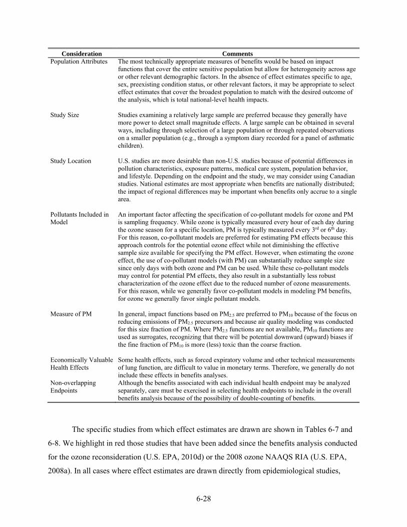
6-28
Consideration Comments Population Attributes The most technically appropriate measures of benefits would be based on impact
functions that cover the entire sensitive population but allow for heterogeneity across age or other relevant demographic factors. In the absence of effect estimates specific to age, sex, preexisting condition status, or other relevant factors, it may be appropriate to select effect estimates that cover the broadest population to match with the desired outcome of the analysis, which is total national-level health impacts.
Study Size Studies examining a relatively large sample are preferred because they generally have more power to detect small magnitude effects. A large sample can be obtained in several ways, including through selection of a large population or through repeated observations on a smaller population (e.g., through a symptom diary recorded for a panel of asthmatic children).
Study Location U.S. studies are more desirable than non-U.S. studies because of potential differences in pollution characteristics, exposure patterns, medical care system, population behavior, and lifestyle. Depending on the endpoint and the study, we may consider using Canadian studies. National estimates are most appropriate when benefits are nationally distributed; the impact of regional differences may be important when benefits only accrue to a single area.
Pollutants Included in Model
An important factor affecting the specification of co-pollutant models for ozone and PM is sampling frequency. While ozone is typically measured every hour of each day during the ozone season for a specific location, PM is typically measured every 3rd or 6th day. For this reason, co-pollutant models are preferred for estimating PM effects because this approach controls for the potential ozone effect while not diminishing the effective sample size available for specifying the PM effect. However, when estimating the ozone effect, the use of co-pollutant models (with PM) can substantially reduce sample size since only days with both ozone and PM can be used. While these co-pollutant models may control for potential PM effects, they also result in a substantially less robust characterization of the ozone effect due to the reduced number of ozone measurements. For this reason, while we generally favor co-pollutant models in modeling PM benefits, for ozone we generally favor single pollutant models.
Measure of PM In general, impact functions based on PM2.5 are preferred to PM10 because of the focus on reducing emissions of PM2.5 precursors and because air quality modeling was conducted for this size fraction of PM. Where PM2.5 functions are not available, PM10 functions are used as surrogates, recognizing that there will be potential downward (upward) biases if the fine fraction of PM10 is more (less) toxic than the coarse fraction.
Economically Valuable Health Effects
Some health effects, such as forced expiratory volume and other technical measurements of lung function, are difficult to value in monetary terms. Therefore, we generally do not include these effects in benefits analyses.
Non-overlapping Endpoints
Although the benefits associated with each individual health endpoint may be analyzed separately, care must be exercised in selecting health endpoints to include in the overall benefits analysis because of the possibility of double-counting of benefits.
The specific studies from which effect estimates are drawn are shown in Tables 6-7 and
6-8. We highlight in red those studies that have been added since the benefits analysis conducted
for the ozone reconsideration (U.S. EPA, 2010d) or the 2008 ozone NAAQS RIA (U.S. EPA,
2008a). In all cases where effect estimates are drawn directly from epidemiological studies,

6-29
standard errors are used as a partial representation of the uncertainty in the size of the effect
estimate. Table 6-9 summarizes those health endpoints and studies we have included in
quantitative analyses supporting uncertainty characterization.
Table 6-7. Health Endpoints and Epidemiological Studies Used to Quantify Ozone-Related
Health Impacts a
Endpoint Study Study
Population
Relative Risk or Effect Estimate (β) (with 95th Percentile Confidence
Interval or SE) Premature Mortality
Premature mortality—short-term
Smith et al. (2009) All ages
β = 0.00032 (0.00008) Zanobetti and Schwartz (2008)
β = 0.00051 (0.00012)
Premature respiratory mortality-long-term
Jerrett et al. (2009) >29 years
β = 0.003971 (0.00133)
Hospital Admissions
Respiratory Pooled estimate: Katsouyanni et al. (2009)
> 65 years
β = 0.00064 (0.00040) penalized splines
Asthma-related emergency department
visits
Pooled estimate: Glad et al. (2012)
0-99 years
β = 0.00306 (0.00117)
Ito et al. (2007) β = 0.00521 (0.00091) Mar and Koenig (2010)
β = 0.01044 (0.00436) (0-17 yr olds) β = 0.00770 (0.00284) (18-99 yr olds)
Peel et al. (2005) β = 0.00087 (0.00053) Sarnat et al. (2013) β = 0.00111 (0.00028) Wilson et al. (2005) RR = 1.022 (0.996 – 1.049) per 25
Other Health Endpoints
Asthma exacerbation Pooled estimate: b Mortimer et al. (2002) Schildcrout et al. (2006)
6–18 years
β = 0.00929 (0.00387) β = 0.00222 (0.00282)
School loss days
Pooled estimate: Chen et al. (2000) 5-17 years
β = 0.015763 (0.004985)
Gilliland et al. (2001) β = 0.007824 (0.004445) Acute respiratory
symptoms (MRAD) Ostro and Rothschild (1989) 18–65 years
β = 0.002596 (0.000776)
a Studies highlighted in red represent updates incorporated since the 2008 ozone NAAQS RIA (U.S. EPA, 2008a). b The original study populations were 5 to 12 years for Schildcrout et al. (2006) and 5-9 years for the Mortimer et al. (2002) study. Based on advice from the SAB-HES, we extended the applied population to 6-18 years for all three studies, reflecting the common biological basis for the effect in children in the broader age group. See: U.S. EPA-SAB (2004a) and NRC (2002).
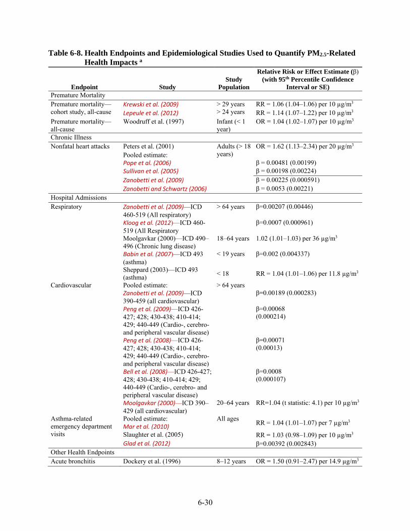
6-30
Table 6-8. Health Endpoints and Epidemiological Studies Used to Quantify PM2.5-Related Health Impacts a
Endpoint Study Study
Population
Relative Risk or Effect Estimate (β) (with 95th Percentile Confidence
Interval or SE) Premature Mortality Premature mortality—cohort study, all-cause
Krewski et al. (2009) > 29 years > 24 years
RR = 1.06 (1.04–1.06) per 10 µg/m3 Lepeule et al. (2012) RR = 1.14 (1.07–1.22) per 10 µg/m3
Premature mortality—all-cause
Woodruff et al. (1997) Infant (< 1 year)
OR = 1.04 (1.02–1.07) per 10 µg/m3
Chronic Illness Nonfatal heart attacks Peters et al. (2001) Adults (> 18
years) OR = 1.62 (1.13–2.34) per 20 µg/m3
Pooled estimate: Pope et al. (2006)
β = 0.00481 (0.00199)
Sullivan et al. (2005) β = 0.00198 (0.00224) Zanobetti et al. (2009) β = 0.00225 (0.000591) Zanobetti and Schwartz (2006) β = 0.0053 (0.00221)
Hospital Admissions Respiratory Zanobetti et al. (2009)—ICD
460-519 (All respiratory) > 64 years β=0.00207 (0.00446)
Kloog et al. (2012)—ICD 460-519 (All Respiratory
β=0.0007 (0.000961)
Moolgavkar (2000)—ICD 490–496 (Chronic lung disease)
18–64 years 1.02 (1.01–1.03) per 36 µg/m3
Babin et al. (2007)—ICD 493 (asthma)
< 19 years β=0.002 (0.004337)
Sheppard (2003)—ICD 493 (asthma)
< 18 RR = 1.04 (1.01–1.06) per 11.8 µg/m3
Cardiovascular Pooled estimate: Zanobetti et al. (2009)—ICD 390-459 (all cardiovascular)
> 64 years β=0.00189 (0.000283)
Peng et al. (2009)—ICD 426-427; 428; 430-438; 410-414; 429; 440-449 (Cardio-, cerebro- and peripheral vascular disease)
β=0.00068 (0.000214)
Peng et al. (2008)—ICD 426-427; 428; 430-438; 410-414; 429; 440-449 (Cardio-, cerebro- and peripheral vascular disease)
β=0.00071 (0.00013)
Bell et al. (2008)—ICD 426-427; 428; 430-438; 410-414; 429; 440-449 (Cardio-, cerebro- and peripheral vascular disease)
β=0.0008 (0.000107)
Moolgavkar (2000)—ICD 390–429 (all cardiovascular)
20–64 years RR=1.04 (t statistic: 4.1) per 10 µg/m3
Asthma-related emergency department visits
Pooled estimate: Mar et al. (2010)
All ages RR = 1.04 (1.01–1.07) per 7 µg/m3
Slaughter et al. (2005) RR = 1.03 (0.98–1.09) per 10 µg/m3 Glad et al. (2012) β=0.00392 (0.002843)
Other Health Endpoints Acute bronchitis Dockery et al. (1996) 8–12 years OR = 1.50 (0.91–2.47) per 14.9 µg/m3

6-31
Asthma exacerbations Pooled estimate: Ostro et al. (2001) (cough, wheeze, shortness of breath) b
6–18 years b OR = 1.03 (0.98–1.07) OR = 1.06 (1.01–1.11) OR = 1.08 (1.00–1.17) per 30 µg/m3
Mar et al. (2004) (cough, shortness of breath)
RR = 1.21 (1–1.47) per RR = 1.13 (0.86–1.48) per 10 µg/m3
Work loss days Ostro (1987) 18–65 years β=0.0046 (0.00036) Acute respiratory symptoms (MRAD)
Ostro and Rothschild (1989) (Minor restricted activity days)
18–65 years β=0.00220 (0.000658)
Upper respiratory symptoms
Pope et al. (1991) Asthmatics, 9–11 years
1.003 (1–1.006) per 10 µg/m3
Lower respiratory symptoms
Schwartz and Neas (2000) 7–14 years OR = 1.33 (1.11–1.58) per 15 µg/m3
a Studies highlighted in red represent updates incorporated since the ozone NAAQS RIA (U.S. EPA, 2008a). These updates were introduced in the PM NAAQS RIA (U.S. EPA, 2012c). b The original study populations were 8 to 13 years for the Ostro et al. (2001) study and 7 to 12 years for the Mar et al. (2004) study. Based on advice from the SAB-HES, we extended the applied population to 6-18 years, reflecting the common biological basis for the effect in children in the broader age group. See: U.S. EPA-SAB (2004a,b) and NRC (2002). Table 6-9. Health Endpoints and Epidemiological Studies Used to Quantify Ozone-Related
Health Impacts in Quantitative Analyses Supporting Uncertainty Characterization a
Endpoint Study Study
Population
Effect Estimate (β) (with 95th Percentile Confidence Interval)
Premature Mortality Premature respiratory mortality - long-term
Jerrett et al. (2009)‐based models:
> 29 years
‐ non‐threshold ozone only (86 cities) β=0.00266 (0.000969) ‐ non‐threshold ozone only (96 cities) β=0.00286 (0.000942) ‐ threshold 40 ppbb β=0.00312 (0.00096) ‐ threshold 45 ppb β=0.00336 (0.001) ‐ threshold 50 ppb β=0.00356 0.00106) ‐ threshold 55 ppb β=0.00417 (0.00118) ‐ threshold 56 ppb β=0.00432 (0.00121) ‐ threshold 60 ppb β=0.00402 (0.00137)
Premature mortality - short-term
Smith et al. (2009) (co‐pollutant model with PM10)
All ages
β=0.00026 (0.00017) Bell et al. (2005) β=0.00080 (0.00021) Levy et al. (2005) β=0.00112 (0.00018) Bell et al. (2004) β=0.00026 (0.00009) Ito et al. (2005) β=0.00117 (0.00024) Schwartz et al. (2005) β=0.00043 (0.00015) Huang et al. (2005) β=0.00026 (0.00009)
a Studies highlighted in red represent updates incorporated since the 2008 ozone NAAQS RIA (U.S. EPA, 2008a). b All threshold models are ozone-only and based on the full 96 city dataset.
6-32
6.6.3.1 Ozone Exposure Metric
Both the NMMAPS analysis and the individual time series studies upon which the meta-
analyses were based use the 24-hour average or 1-hour maximum ozone concentrations as
exposure metrics. The 24-hour average is not the most relevant ozone exposure metric to
characterize population-level exposure. Given that the majority of the people tend to be outdoors
during the daylight hours and concentrations are highest during the daylight hours, the 24-hour
average metric is not appropriate. Moreover, the 1-hour maximum metric uses an exposure
window different than that used for the current ozone NAAQS. A more biologically relevant
metric, and the one used in the ozone NAAQS since 1997, is the maximum daily 8-hour average
ozone. Thus, we converted ozone mortality health impact functions that use a 24-hour average or
1-hour maximum ozone metric to maximum 8-hour average ozone concentration using standard
conversion functions.
This practice is consistent with the form of the current ozone standard. This conversion
does not affect the relative magnitude of the health impact function from a mathematical
standpoint. An equivalent change in the 24-hour average, 1-hour maximum and 8-hour
maximum will provide the same overall change in incidence of a health effect.135 The conversion
ratios are based on observed relationships between the 24-hour average and 8-hour maximum
ozone values. For example, in the Bell et al., 2004 analysis of ozone-related premature mortality,
the authors found that the relationship between the 24-hour average, the 8-hour maximum, and
the 1-hour maximum was 2:1.5:1, so that the derived health impact effect estimate based on the
1-hour maximum should be half that of the effect estimate based on the 24-hour values (and the
8-hour maximum three-quarters of the 24-hour effect estimate).
As part of the quantitative uncertainty analyses for this benefits analysis, we apply
national effect estimates based on the pooled multi-city results reported in Bell et al. (2004) and
the three meta-analysis studies. Bell et al. (2004), Bell et al. (2005), Levy et al. (2005), and Ito et
135 However, different ozone metrics may not be well correlated (from either a spatial or temporal standpoint) within
a given geographic area, which means that application of ratio-converted effect estimates for the same endpoint can result in different incidence estimates for the same location under certain conditions. This introduces uncertainty into the use of these ratio-adjusted effect estimates (see Appendix 6A).

6-33
al. (2005) all provide national conversion ratios between daily average and 8-hour and 1-hour
maxima, based on national data.
6.6.3.2 Ozone Premature Mortality Effect Coefficients
Mortality Effect Coefficients for Short-term Ozone Exposure. The overall body of
evidence indicates that there is likely to be a causal relationship between short-term ozone
exposure and premature mortality, even as we are mindful of the uncertainty associated with the
shape of the concentration response curve at lower ozone concentrations. (U.S. EPA, 2013a,
page 1-7). The 2013 ozone ISA concludes that the evidence suggests that ozone effects are
independent of the relationship between PM and mortality. (U.S. EPA, 2013a). However, the
ISA notes that the interpretation of the potential confounding effects of PM on ozone-mortality
risk estimates requires caution due to the PM sampling schedule (in most cities) which limits the
overall sample size available for evaluating potential confounding of the ozone effect by PM
(U.S. EPA 2013a).136 Below we describe the evolution of EPA’s understanding of the evidence
supporting causality related to short-term ozone exposure and mortality (including
recommendations provided to EPA by the NAS).
These observations are consistent with prior recommendations to the EPA by the NAS
regarding the quantification and valuation of ozone-related short-term mortality (NRC, 2008).
Chief among the NAS recommendations was that “…short-term exposure to ambient ozone is
likely to contribute to premature deaths” and the committee recommended that “ozone-related
mortality be included in future estimates of the health benefits of reducing ozone exposures…”
The NAS also recommended that “…the greatest emphasis be placed on the multi-city and
NMMAPS studies without exclusion of the meta-analyses” (NRC, 2008). In addition, NAS
recommended that EPA “should give little or no weight to the assumption that there is no causal
association between estimated reductions in premature mortality and reduced ozone exposure”
(NRC, 2008). In 2010, the Health Effects Subcommittee of the Advisory Council on Clean Air
Compliance Analysis, while reviewing EPA’s The Benefits and Costs of the Clean Air Act 1990
136 Consequently, as noted later in this section, while we have used a single-pollutant model in generating short-term ozone-related mortality benefits for this RIA, we have included a co-pollutants model as a sensitivity analysis to address potential uncertainty associated with this assumption of an independent ozone mortality effect.

6-34
to 2020 (U.S. EPA, 2011a), also confirmed the NAS recommendation to include ozone mortality
benefits (U.S. EPA-SAB, 2010a).
In view of the findings of the ozone ISA, the NAS panel, the SAB-HES panel, and the
CASAC panel, we estimate ozone-related premature mortality for short-term exposure in the
core health effects analysis using effect coefficients from the Smith et al. (2009) NMMAPS
analysis and the Zanobetti and Schwartz (2008) multi-city study with several additional studies
as part of the quantitative uncertainty analysis. CASAC supported using the Smith et al. (2009)
and Zanobetti and Schwartz (2008) studies for the ozone HREA (U.S. EPA-SAB, 2012, 2014),
and these are multi-city studies published more recently (as compared with other multi-city
studies or meta-analyses included in the quantitative uncertainty analyses – see discussion
below).
Smith et al. (2009) reanalyzed the NMMAPS dataset, evaluating the relationship between
short-term ozone exposure and mortality.137 While this study reproduces the core national-scale
estimates presented in Bell et al. (2004), it also explored the sensitivity of the mortality effect to
different model specifications including (a) regional versus national Bayes-based adjustment,138
(b) co-pollutant models considering PM10, (c) all-year versus ozone-season based estimates, and
(d) consideration of a range of ozone metrics, including the daily 8-hour max. In addition, the
Smith et al. (2009) study did not use the trimmed mean approach employed in the Bell et al.
(2004) study in preparing ozone monitor data.139 In selecting among the effect estimates from
Smith et al. (2009), we focused on an ozone-only estimate for non-accidental mortality using the
137 In previous RIAs involving ozone, we have used Bell et al. (2004) as the basis for modeling short-term exposure-related mortality. However, for reasons presented here and outlined in section 7.3.2 of the final REA completed in support of the ozone review (U.S. EPA 2014b), we have substituted Smith et al. (2009) as the basis for effect estimates used in modeling this endpoint for both the REA and the benefit analysis described here. The Smith et al. (2009) effect estimate used in this RIA (0.00032, see Table 6-7) is about 22% larger than the Bell et al. (2004) effect estimate (0.000261, BenMAP-CE standard health functions, U.S. EPA 2015a). 138 In Bayesian modeling, effect estimates are “updated” from an assumed prior value using observational data. In the Smith et al. (2009) approach, the prior values are either a regional or national mean of the individual effect estimates obtained for each individual city. The Bayesian adjusted city-specific effect estimates are then calculated by updating the selected prior value based on the relative precision of each city-specific estimate and the variation observed across all city-specific individual effect estimates. City-specific estimates are pulled towards the prior value if they have low precision and/or if there is low overall variation across estimates. City-specific estimates are given less adjustment if they are precisely estimated and/or there is greater overall variation across estimates. 139 There are a number of concerns regarding the trimmed mean approach including (1) the potential loss of temporal variation in the data when the approach is used (this could impact the size of the effect estimate), and (2) a lack of complete documentation for the approach, which prevents a full reviewing or replication of the technique.

6-35
8-hour max metric for the warmer ozone season.140 For the quantitative uncertainty analysis, we
included a co-pollutant model (ozone and PM10) from Smith et al. (2009) for all-cause mortality,
using the 8-hour max ozone metric for the ozone season. Using a single pollutant model for the
core analysis and the co-pollutant model in the quantitative uncertainty analysis reflects our
concern that the reduced sampling frequency for days with co-pollutant measurements (1/3 and
1/6) could affect the ability of the study to characterize the ozone effect. This choice is consistent
with the ozone ISA, which concludes that ozone effects are likely to be independent of the
relationship between PM and mortality (U.S. EPA, 2013a).
The Zanobetti and Smith (2008) study evaluated the relationship between ozone exposure
(using an 8-hour mean metric for the warm season June-August) and all-cause mortality in 48
U.S. cities using data collected between 1989 and 2000. The study presented single pollutant C-
R functions based on shorter (0-3 day) and longer (0-20 day) lag structures, with the comparison
of effects based on these different lag structures being a central focus of the study. We used the
shorter day lag based C-R function since this had the strongest effect and tighter confidence
interval. We converted the effect estimate from an 8-hour mean metric to an equivalent effect
estimate based on an 8-hour max. To do this, we used the ozone metric approach wherein the
original effect estimate (and standard error) is multiplied by the appropriate ozone metric
adjustment ratio.141
Mortality Effect Coefficient for Long-term Ozone Exposure. Although previous
advice provided by the SAB-HES was to include long-term ozone exposure-related mortality
only as part of a quantitative uncertainty analysis, based on the more recent ISA, CASAC advice,
140 The effect estimates used for both the core and uncertainty were obtained from Smith et al., 2009. Specifically, for the core analysis, we used the national-scale ozone-only summer 8-hour max based effect estimate and standard error (Smith et al., 2009 Table 1, row seven, columns seven and eight) and for the uncertainty analysis, we included the two-pollutant model summer 8-hour max effect estimate and standard error (Smith et al., 2009 Table 1, row ten, columns seven and eight). The model results presented in Table 1 of Smith et al. (2009) represent percentage rise in mortality per 10 ppb rise in the relevant metric of ozone and consequently these had to be adjusted to represent a factor increase per unit ozone. 141 These adjustment ratios are created by (a) obtaining summary air quality (composite monitor values) for each urban study area/ozone season combination reflected in the original epidemiology study, (b) calculating the ratio of the 8-hour max to the study-specific air metric (for each of the urban study areas), and (c) taking the average of these urban-study area ratios. Ratio adjustment of the effect estimate does introduce uncertainty into the benefits estimates generated using these adjusted effect estimates; however, adjustments of relatively similar metrics (e.g., 8-hour max and 8-hour mean), as is the case with the Zanobetti and Schwartz (2008) study, are likely to introduce less uncertainty than adjustments for more disparate ratios (e.g., 24-hour or 1-hour max ratios to 8-hour max equivalents).

6-36
and HREA, the current RIA estimated long-term ozone exposure-related respiratory mortality
incidence in the core analysis.142 Support for modeling long-term exposure-related mortality
incidence comes from the ozone ISA as well as recommendations provided by CASAC in their
review of the ozone HREA (U.S. EPA-SAB, 2014, p. 3 and 9), despite the lower confidence in
quantifying this endpoint because the ISA’s consideration of this endpoint is primarily based on
one study (Jerrett et al, 2009), though that study is well designed, and because of the uncertainty
in that study about the existence and identification of a potential threshold in the concentration-
response function. Whereas the ozone ISA concludes that evidence is suggestive of a causal
association between total mortality and long-term ozone exposure, specifically with regard to
respiratory health effects (including mortality), the ISA concludes that there is likely to be a
causal association (U.S. EPA, 2013a). Consistent with the ozone HREA, we use Jerrett et al.
(2009) to estimate premature respiratory mortality from long-term ozone exposure. In review of
the ozone HREA, CASAC concluded that “Jerrett et al. (2009) is an appropriate study to use at
this time as the basis for the long-term mortality risk estimates given its adequacy and the lack of
alternative data.” (U.S. EPA-SAB, 2014).
The Jerrett et al. (2009) study was the first to explore the relationship between long-term
ozone exposure and respiratory mortality (rather than other causes of mortality). Jerrett et al.
(2009) exhibits a number of strengths including (a) the study was based on the 1.2 million
participant American Cancer Society cohort drawn from all 50 states, DC, and Puerto Rico
(included ozone data from 1977, 5 years before enrollment in the cohort began, to 2000); (b) it
included co-pollutant models that controlled for PM2.5; and (c) it explored the potential for a
threshold concentration associated with the long-term mortality endpoint. However, attributes of
this study affect how we interpret the long-term exposure-related respiratory mortality estimates.
First, while CASAC notes that Jerrett et al. (2009) was well designed, it is a single study and
provides the only quantitative basis for estimating this endpoint. By comparison, we estimate
short-term exposure-related mortality risk using several studies.
142 As explained in section 6.3, because we do not have information on the cessation lag for premature mortality from long-term ozone exposure, we do not include the monetized benefits in the core analysis. Instead, monetized benefits associated with long-term ozone-related respiratory mortality are included as a sensitivity analysis (see Appendix 5B, section 5B.2).
6-37
The quantitative uncertainty analysis take into consideration the potential existence and
location of a threshold in the C-R function relating mortality and long-term ozone
concentrations, which can greatly affect the results. CASAC concluded, “it is not clear whether
the 56 ppb threshold model is a better predictor of respiratory mortality than when using a linear
model for the Jerrett et al. data” (U.S. EPA-SAB, 2014, p. 13-14)
Reflecting this CASAC advice in the context of the HREA, we estimate long-term
exposure-related respiratory mortality using a non-threshold co-pollutant model (with PM2.5)
from Jerrett et al. (2009). Because the Jerrett et al. (2009) study uses seasonal average metrics
(rather than shorter single day or multi-day lagged models as with time series studies studies),
co-pollutants models obtained from Jerrett et al., (2009) are not affected by the lower PM2.5
sampling rates. Using a co-pollutant model is consistent with this study applying seasonal
average metrics that are insensitive to co-pollutant monitoring for PM2.5. The effect estimates
used to model long-term ozone-attributable mortality are calculated using a seasonal average of
peak (1-hour maximum) measurements. These long-term exposure metrics can be viewed as
long-term exposures to daily peak ozone over the warmer months, as compared with annual
average levels such as are used in PM benefits. Therefore, combining long-term and short-term
ozone-attributable mortality estimates could lead to double counting. Estimates of short-term
ozone mortality are for all-causes, while estimates of long-term ozone mortality are for
respiratory-related mortality only.
Quantitative uncertainty Analysis: Alternate Mortality Effect Coefficients for
Short-term Ozone Exposure. Although we believe the evidence supports an ozone-only effect
on short-term exposure-related mortality (as supported by the ozone ISA), we recognize
limitations in the ability of studies to explore copollutants effects due to lower sampling
frequency for PM relative to ozone. For that reason, we conduct a quantitative uncertainty
analysis using the co-pollutants model (with PM10) from Smith et al. (2009).
Quantitative uncertainty Analysis: Threshold-Based Effect Coefficients for Long-
term Ozone Exposure. Consistent with the ozone HREA (U.S. EPA, 2014b), we explore the
sensitivity of estimated ozone-related premature mortality to a concentration threshold using the
6-38
Jerrett et al. (2009) study.143 In their memo clarifying the results of their study (see Sasser, 2014),
the authors note that in terms of goodness of fit, long-term health risk models including ozone
clearly performed better than models without ozone. This supports the authors’ assertion that
improved predictions of respiratory mortality are generated when ozone is included in the model.
In exploring different functional forms, they report that the model including a threshold at 56 ppb
had the lowest log-likelihood value of all models evaluated (i.e., linear models and models
including thresholds ranging from 40-60 ppb), and thus provided the best overall statistical fit to
the data. However, they also note that it is not clear whether the 56 ppb threshold model is a
better predictor of respiratory mortality than when using a linear (no-threshold) model for this
dataset. Using one statistical test, the model with a threshold at 56 ppb was determined to be
statistically superior to the linear model. Using another, more stringent test, none of the threshold
models considered were statistically superior to the linear model. Under the less stringent test,
although the threshold model produces a statistically superior prediction than the linear model,
there is uncertainty about the specific location of the threshold, if one exists. This is because the
confidence intervals on the model predictions indicate that a threshold could exist anywhere
from 0 to 60 ppb. The authors conclude that considerable caution should be exercised in using
any specific threshold, particularly when the more stringent statistical test indicates there is no
significantly improved prediction.
Based on this additional information from the authors (Sasser, 2014), we have chosen to
reflect the uncertainty about the existence and location of a potential threshold by estimating
mortality attributable to long-term ozone exposures using a range of threshold-based effect
estimates as quantitative uncertainty analyses. Specifically, we generate additional long-term risk
results using unique risk models that include a range of thresholds from 40 ppb to 60 ppb in 5
ppb increments, while also including a model with a threshold equal to 56 ppb, which had the
lowest log likelihood value for all models examined.144 In addition to exploring the impact of
potential thresholds, as part of the quantitative uncertainty analysis we explore the impact of
143 The approach in the ozone HREA to explore the potential for thresholds related to long-term exposure-related
mortality is described in Sasser (2014). That memorandum also describes additional data obtained from the authors of Jerrett et al. (2009) to support modeling potential thresholds.
144 There is a separate effect estimate (and associated standard error) for each of the fitted threshold models estimated in Jerrett et al. (2009). As a result, the sensitivity of estimated mortality attributable to long-term ozone concentrations is affected by both the assumed threshold level (below which there is no effect of ozone) and the effect estimate applied to ozone concentrations above the threshold.

6-39
using ozone-only (non-threshold) models in estimating long-term exposure-related respiratory
mortality.145
6.6.3.3 PM2.5 Premature Mortality Coefficients
The co-benefits associated with NOx reductions made in the models to achieve ozone
reductions are estimated in this RIA using methods consistent with those develop for the RIA for
the final 2012 PM2.5 NAAQS. Below we provide additional background for readers who are not
familiar with the PM2.5 literature that drives the approach developed for the 2012 PM2.5 NAAQS
and employed by EPA since then.
PM2.5 Mortality Effect Coefficients for Adults. A substantial body of published
scientific literature documents the association between elevated PM2.5 concentrations and
increased premature mortality (U.S. EPA, 2009b). This body of literature reflects thousands of
epidemiology, toxicology, and clinical studies. The PM ISA completed as part of the most recent
review of the PM NAAQS, which was twice reviewed by the SAB-CASAC (U.S. EPA-SAB,
2009a, 2009b), concluded that there is a causal relationship between mortality and both long-
term and short-term exposure to PM2.5 based on the entire body of scientific evidence (U.S. EPA,
2009b). The size of the mortality effect estimates from epidemiological studies, the serious
nature of the effect itself, and the high monetary value ascribed to prolonging life make mortality
risk reduction the most significant health endpoint quantified in this analysis.
Researchers have found statistically significant associations between PM2.5 and
premature mortality using different types of study designs. Time-series methods have been used
to relate short-term (often day-to-day) changes in PM2.5 concentrations and changes in daily
mortality rates up to several days after a period of exposure to elevated PM2.5 concentrations.
Cohort methods have been used to examine the potential relationship between community-level
PM2.5 exposures over multiple years (i.e., long-term exposures) and community-level annual
mortality rates that have been adjusted for individual level risk factors. When choosing between
145 The set of ozone-only non-threshold effect estimates include (a) a value based on the 86 cities for which there are
co-pollutant monitoring data for both ozone and PM2.5 (this is best compared with the core estimate based on the co-pollutant non-threshold model), and (b) a value based on the 96 cities for which there is PM2.5 data (these 96 cities were used in developing the threshold-based effect estimates used in the analysis).

6-40
using short-term studies or cohort studies for estimating mortality benefits, cohort analyses are
thought to capture more of the public health impact of exposure to air pollution over time
because they account for the effects of long-term exposures, as well as some fraction of short-
term exposures (Kunzli et al., 2001; NRC, 2002). The National Research Council (NRC) stated
that “it is essential to use the cohort studies in benefits analysis to capture all important effects
from air pollution exposure” (NRC, 2002, p. 108). The NRC further noted that “the overall effect
estimates may be a combination of effects from long-term exposure plus some fraction from
short-term exposure. The amount of overlap is unknown” (NRC, 2002, p. 108-9). To avoid
double counting, we focus on applying the risk coefficients from the long-term cohort studies in
estimating the mortality impacts of reductions in PM2.5.
Over the last two decades, several studies using “prospective cohort” designs have been
published that are consistent with the earlier body of literature. Two prospective cohort studies,
often referred to as the Harvard “Six Cities Study” (Dockery et al., 1993; Laden et al., 2006;
Lepeule et al., 2012) and the “American Cancer Society” or “ACS study” (Pope et al., 1995;
Pope et al., 2002; Pope et al., 2004; Krewski et al., 2009), provide the most extensive analyses of
ambient PM2.5 concentrations and mortality. These studies have found consistent relationships
between fine particle indicators and premature mortality across multiple locations in the United
States. The credibility of these two studies is further enhanced by the fact that the initial
published studies (Pope et al., 1995; Dockery et al., 1993) were subject to extensive
reexamination and reanalysis by an independent team of scientific experts commissioned by the
Health Effects Institute (HEI) and by a Special Panel of the HEI Health Review Committee
(Krewski et al., 2000). Publication of studies confirming and extending the findings of the 1993
Six Cities Study and the 1995 ACS study using more recent air quality data and a longer follow-
up period for the ACS cohort provides additional validation of the findings of these original
studies (Pope et al., 2002, 2004; Laden et al., 2006; Krewski et al., 2009; Lepeule et al., 2012).
The SAB-HES also supported using these two cohorts for analyses of the benefits of PM
reductions, and concluded, “the selection of these cohort studies as the underlying basis for PM
mortality benefit estimates [is] a good choice. These are widely cited, well studied and
extensively reviewed data sets” (U.S. EPA-SAB, 2010a). As both the ACS and Six Cities studies
have inherent strengths and weaknesses, we present benefits estimates using relative risk
estimates from the most recent extended reanalysis of these cohorts (Krewski et al., 2009;
6-41
Lepeule et al., 2012). Presenting results using both ACS and Six Cities is consistent with other
recent RIAs (e.g., U.S. EPA, 2010c, 2011a, 2011c). The PM ISA concludes that the ACS and Six
Cities cohorts provide the strongest evidence of the association between long-term PM2.5
exposure and premature mortality with support from a number of additional cohort studies
(described below).
The extended analyses of the ACS cohort data (Krewski et al., 2009) refined the earlier
ACS studies by (a) extending the follow-up period by 2 years to the year 2000, for a total of 18
years; (b) incorporating almost double the number of urban areas; (c) addressing confounding by
spatial autocorrelation by incorporating ecological, or community-level, co-variates; and (d)
performing an extensive spatial analysis using land use regression modeling in two large urban
areas. These enhancements make this analysis well-suited for the assessment of mortality risk
from long-term PM2.5 exposures for the EPA’s benefits analyses.
In 2009, the SAB-HES again reviewed the choice of mortality risk coefficients for
benefits analysis, concluding that “[t]he Krewski et al. (2009) findings, while informative, have
not yet undergone the same degree of peer review as have the aforementioned studies. Thus, the
SAB-HES recommends that EPA not use the Krewski et al. (2009) findings for generating the
Primary Estimate” (U.S. EPA-SAB, 2010a). Since this time, the Krewski et al. (2009) has
undergone additional peer review, which we believe strengthens the support for including this
study in this RIA. For example, the PM ISA (U.S. EPA, 2009b) included this study among the
key mortality studies. In addition, the risk assessment supporting the PM NAAQS (U.S. EPA,
2010b) used risk coefficients drawn from the Krewski et al. (2009) study, the most recent
reanalysis of the ACS cohort data. The PM risk assessment cited a number of advantages that
informed the selection of the Krewski et al. (2009) study as the source of the core effect
estimates, including the extended period of observation, the rigorous examination of model
forms and effect estimates, the coverage for ecological variables, and the large dataset with over
1.2 million individuals and 156 MSAs (U.S. EPA, 2010b). The CASAC also provided extensive
peer review of the PM risk assessment and supported the use of effect estimates from this study
(U.S. EPA-SAB, 2009a, b, 2010b).

6-42
Consistent with the PM risk assessment (U.S. EPA, 2010b) which was reviewed by the
CASAC (U.S. EPA-SAB, 2009a, b), we use the all-cause mortality risk estimate based on the
random-effects Cox proportional hazard model that incorporates 44 individual and 7 ecological
covariates (RR=1.06, 95% confidence intervals 1.04–1.08 per 10 µg/m3 increase in PM2.5). The
relative risk estimate (1.06 per 10 µg/m3 increase in PM2.5) is identical to the risk estimate drawn
from the earlier Pope et al. (2002) study, though the confidence interval around the Krewski et
al. (2009) risk estimate is tighter.
In the most recent Six Cities study, which was published after the last SAB-HES review,
Lepeule et al. (2012) evaluated the sensitivity of previous Six Cities results to model
specifications, lower exposures, and averaging time using eleven additional years of cohort
follow-up that incorporated recent lower exposures. The authors found significant associations
between PM2.5 exposure and increased risk of all-cause, cardiovascular and lung cancer
mortality. The authors also concluded that the C-R relationship was linear down to PM2.5
concentrations of 8 μg/m3 and that mortality rate ratios for PM2.5 fluctuated over time, but
without clear trends, despite a substantial drop in the sulfate fraction. We use the all-cause
mortality risk estimate based on a Cox proportional hazard model that incorporates 3 individual
covariates. (RR=1.14, 95% confidence intervals 1.07–1.22 per 10 µg/m3 increase in PM2.5). The
relative risk estimate is slightly smaller than the risk estimate drawn from Laden et al. (2006),
with relatively smaller confidence intervals.
Given that monetized benefits associated with PM2.5 are driven largely by reductions in
premature mortality, it is important to characterize the uncertainty in this endpoint. In order to do
so, we utilize the results of an expert elicitation sponsored by the EPA and completed in 2006
(Roman et al., 2008; IEc, 2006). The results of that expert elicitation can be used as a
characterization of uncertainty in the C-R functions. The co-benefits results derived from expert
elicitation is discussed in Appendix 6B (section 6B.4).
PM2.5 Mortality Effect Coefficients for Infants. In addition to the adult mortality
studies described above, several studies show an association between PM exposure and
premature mortality in children under 5 years of age.146 The PM ISA states that less evidence is
146 For the purposes of this analysis, we only calculate benefits for infants age 0–1, not all children under 5 years old.

6-43
available regarding the potential impact of PM2.5 exposure on infant mortality than on adult
mortality and the results of studies in several countries include a range of findings with some
finding significant associations. Specifically, the PM ISA concluded that evidence exists for a
stronger effect at the post-neonatal period and for respiratory-related mortality, although this
trend is not consistent across all studies. In addition, compared to avoided premature mortality
estimated for adults, avoided premature mortality for infants are significantly smaller because the
number of infants in the population is much smaller than the number of adults and the
epidemiology studies on infant mortality provide smaller risk coefficients associated with
exposure to PM2.5.
In 2004, the SAB-HES noted the release of the WHO Global Burden of Disease Study
focusing on ambient air, which cites several recently published time-series studies relating daily
PM exposure to mortality in children (U.S. EPA-SAB, 2004). With regard to the cohort study
conducted by Woodruff et al. (1997), the SAB-HES noted several strengths of the study,
including the use of a larger cohort drawn from a large number of metropolitan areas and efforts
to control for a variety of individual risk factors in infants (e.g., maternal educational level,
maternal ethnicity, parental marital status, and maternal smoking status). Based on these
findings, the SAB-HES recommended that the EPA incorporate infant mortality into the primary
benefits estimate and that infant mortality be evaluated using an impact function developed from
the Woodruff et al. (1997) study (U.S. EPA-SAB, 2004).
In 2010, the SAB-HES again noted the increasing body of literature relating infant
mortality and PM exposure and supported the inclusion of infant mortality in the monetized
benefits (U.S. EPA-SAB, 2010a). The SAB-HES generally supported the approach of estimating
infant mortality based on Woodruff et al. (1997) but also noted that a more recent study by
Woodruff et al. (2006) continued to find associations between PM2.5 and infant mortality in
California. The SAB-HES also noted, “when PM10 results are scaled to estimate PM2.5 impacts,
the results yield similar risk estimates.” Consistent with The Benefits and Costs of the Clean Air
Act 1990 to 2020 (U.S. EPA, 2011a), we continue to rely on the earlier 1997 study in part due to
the national–scale of the earlier study.

6-44
6.6.3.4 Hospital Admissions and Emergency Department Visits
We pool together the incidence estimates using several different studies for many of the
hospital admission endpoints. Some studies have examined the relationship between air pollution
and emergency department (ED) visits. Since most emergency department visits do not result in
an admission to the hospital (i.e., most people going to the emergency department are treated and
return home), we treat hospital admissions and emergency department visits separately, taking
account of the fraction of emergency department visits that are admitted to the hospital.
Specifically, within the baseline incidence rates, we parse out the scheduled hospital visits from
unscheduled ones as well as the hospital visits that originated in the emergency department.
The ozone ISA states that studies consistently found positive associations between short-
term ozone exposures and asthma and COPD hospital admissions and ED visits, with more
limited evidence for pneumonia (U.S. EPA, 2013a). The ISA found no evidence of a threshold
between short term ozone exposure and respiratory hospital admissions and ED visits, although
there is increasing uncertainty at lower ozone concentrations particularly at and below 20 ppb
(U.S. EPA, section 2.5.4.4). The ISA also observes that effect estimates remained robust to
copollutants (U.S. EPA 2013a).
Considering these observation from the ISA and a thoroughly reviewing available
epidemiological studies, we estimate respiratory hospital admissions (for 65-99 year olds) using
an effect estimate obtained from Katsouyanni et al. (2009) and asthma-related emergency room
visits (for all ages) using several single-city studies. Although Katsouyanni et al. (2009) provides
effect estimates specific to the summer season, we adjusted the 1-hour max metric to the
equivalent 8-hour max effect estimates.147 The study provides summer season single pollutant
effect estimates based both on natural and penalized splines. We have re-evaluated the choice of
these models in this final RIA. In contrast to the proposal RIA, where we averaged both the
penalized and natural spline estimates, we decided to focus on the penalized spline model
147 Given that Katsouyanni et al. (2009) included a larger number of cities (14), rather than constructing an air metric
adjustment ratio based on this set of urban study areas, we used a national ratio to adjust effect estimates to represent the 8-hour metric.

6-45
because it displays a higher degree of precision, thus less potential for random error. 148 While
Katsouyanni et al. (2009) included a set of effect estimates based on co-pollutant modeling (with
PM10), but we could not use them because they were based on the full year rather than the
summer season.
A number of studies are available to model respiratory ED visits. Because we do not yet
have the information needed to value this endpoint, we focused on the narrower category of
asthma-related ED visits We used a set of single city studies together with random-effects
pooling to generate a single pooled estimate. The set of single city studies used in this
calculation include: Peel et al. (2005) and Sarnat et al. (2013) both for Atlanta, Wilson et al.
(2005) and Mar and Koenig (2009) for Seattle, Wilson et al. (2005) for Portland, Maine,, Ito et
al. (2007) for New York City, and Glad et al. (2012) for Pittsburgh. We note that of these single
city studies, only the Ito et al. (2007) study included a co-pollutant model (for PM2.5).149 In
addition, two of the studies required adjustments to reflect the 8-hour max air metric.
Specifically, Glad et al. (2012) uses the 1-hour max air metric, while Sarnat et al. (2013) used the
24-hour average metric. Each required the use of air metric ratios to adjust their betas. In
generating a single pooled benefit estimate for this endpoint, we used random/fixed effects
pooling to combine estimates across these single city studies.
The two main groups of hospital admissions estimated in this analysis for PM2.5 are:
respiratory admissions and cardiovascular admissions. There is not sufficient evidence linking
PM2.5 with other types of hospital admissions. Both asthma- and cardiovascular-related visits
have been linked to exposure to PM2.5 in the United States, though as we note below, we are able
to assign an economic value to asthma-related events only. To estimate the effects of PM2.5 air
pollution reductions on asthma-related ER visits, we use the effect estimates from studies of
children 18 and under by Mar et al. (2010), Slaughter et al. (2005), and Glad et al. (2012). The
first two studies examined populations 0 to 99 in Washington, while Glad et al. examined
populations 0-99 in Pittsburgh, Pennsylvania. Mar and colleagues perform their study in
148 We evaluated the impact from this change (i.e., use of the penalized spline model alone as contrasted with an average of estimates generated using both the natural and penalized splines), and this change made a negligible (<<1%) difference in monetized ozone benefits due to the similarity in effect coefficients between the two models. 149 While we have included co-pollutant models as sensitivity analyses for mortality, we did not include separate co-
pollutant models for any of the morbidity endpoints as sensitivity analyses because morbidity endpoint represent a small fraction of the total monetized benefits.

6-46
Tacoma, while Slaughter and colleagues base their study in Spokane. We apply random/fixed
effects pooling to combine evidence across these two studies.
To estimate avoided incidences of cardiovascular hospital admissions associated with
exposure to PM2.5, we used studies by Moolgavkar (2000), Zanobetti et al. (2009), Peng et al.
(2008, 2009) and Bell et al. (2008). Only Moolgavkar (2000) provided a separate effect estimate
for adults 20 to 64, while the remainder estimate risk among adults over 64. Total cardiovascular
hospital admissions are the sum of the pooled estimate for adults over 64 and the single study
estimate for adults 20 to 64. To avoid double-counting benefits from reductions in myocardial
infarctions when applying the impact function for cardiovascular hospital admissions, we first
adjusted the baseline cardiovascular hospital admissions to remove admissions for myocardial
infarctions. We applied equal weights pooling to the multi-city studies assessing risk among
adults over 64 because these studies already incorporated pooling across the city-level estimates.
One potential limitation of our approach is that while the Zanobetti et al. (2009) study assesses
all cardiovascular risk, the Bell et al. (2008), and Peng et al. (2008, 2009) studies estimate a
subset of cardiovascular hospitalizations as well as certain cerebro- and peripheral-vascular
diseases. To address the potential for the pooling of these four studies to produce a biased
estimate, we match the pooled risk estimate with a baseline incidence rate that excludes cerebro-
and peripheral-vascular disease. An alternative approach would be to use the Zanobetti et al.
(2009) study alone, though this would prevent us from drawing upon the strengths of the three
multi-city studies.
To estimate avoided incidences of respiratory hospital admissions associated with PM2.5,
we used a number of studies examining total respiratory hospital admissions as well as asthma
and chronic lung disease. We estimated impacts among three age groups: adults 65 and over,
adults 18 to 64 and children 0 to 17. For adults over 65, the multi-city studies by Zanobetti et al.
(2009) and Kloog et al. (2012) provide effect coefficients for total respiratory hospital
admissions. We pool these two studies using equal weights. Moolgavkar et al. (2003) examines
PM2.5 and chronic lung disease hospital admissions (not including asthma) in Los Angeles,
California among adults 18 to 64. For children 0 to 18, we pool two studies using random/fixed
effects. The first is Babin et al. (2007), which assessed PM2.5 and asthma hospital admissions in
Washington, DC among children 1 to 18; we adjusted the age range for this study to apply to

6-47
children 0 to 18. The second is Sheppard et al. (2003), which assessed PM2.5 and asthma
hospitalizations in Seattle, Washington, among children 0 to 18.
6.6.3.5 Acute Health Events
A number of acute health effects not requiring hospitalization are also associated with
exposure to ozone and PM2.5. The sources for the effect estimates used to quantify these
endpoints are described below.
Asthma exacerbations. For this RIA, we followed the SAB-HES recommendations
regarding asthma exacerbations in developing the core estimate (U.S. EPA-SAB, 2004a).
Although certain studies of acute respiratory events characterize these impacts among only
asthmatic populations, others consider the full population, including both asthmatics and non-
asthmatics. For this reason and to avoid double counting impacts, incidence estimates derived
from studies focused only on asthmatics cannot be added to estimates from studies that consider
the full population. To prevent such double-counting, we estimated the exacerbation of asthma
among children and excluded adults from the calculation. Asthma exacerbations occurring in
adults are assumed to be captured in the general population endpoints, such as work loss days
and minor restricted activity days (MRADs). Finally, we note the important distinction between
the exacerbation of asthma among asthmatic populations and the onset of asthma among
populations not previously suffering from asthma. In this RIA, we quantify the exacerbation of
asthma among asthmatic populations and not the onset of new cases of asthma.
Based on advice from the SAB-HES (U.S. EPA-SAB 2004a), regardless of the age
ranges included in the source epidemiology studies, we extend the applied population to ages 6
to 18, reflecting the common biological basis for the effect in children in the broader age group.
This age range expansion is also supported by NRC (2002, pp. 8, 116).
To characterize asthma exacerbations in children from exposure to ozone, for the
proposed RIA, we selected three multi-city studies (Mortimer et al., 2002; O’Connor et al., 2008;
Schildcrout et al., 2006). All three of these studies required the application of air metric ratios to

6-48
adjust effect estimates to represent the 8-hour max metric.150 In this final RIA, following a final
review of our technical approach, we removed O’Connor (2008) due to concerns about potential
exposure measurement error and residual confounding from meteorological variables in its 19-
day lag structure. Current evidence in the ozone ISA suggests a more immediate effect with
exposure to ozone for respiratory-related effects, such as hospital admissions and emergency
department visits, with additional supporting evidence from studies of respiratory symptoms
(U.S. EPA, 2013a). Consequently, the 19-day lag structure reflected in the O’Connor (2008)
study is not as strongly supported by the evidence as the shorter lag structures associated with the
other two asthma exacerbation studies.151 In generating the asthma exacerbation estimate, we
pool estimates from Mortimer et al. (2012) and Schildcrout et al. (2006) using a random/fixed
effects approach applied within BenMAP-CE (U.S. EPA, 2015a).152
To characterize asthma exacerbations in children from exposure to PM2.5, we selected
two studies (Ostro et al., 2001; Mar et al., 2004) that followed panels of asthmatic children.
Ostro et al. (2001) followed a group of 138 African-American children in Los Angeles for 13
weeks, recording daily occurrences of respiratory symptoms associated with asthma
exacerbations (e.g., shortness of breath, wheeze, and cough). This study found a statistically
significant association between exposure to PM2.5, measured as a 12-hour average, and the daily
prevalence of shortness of breath and wheeze endpoints. Although the association was not
statistically significant for cough, the results were still positive and close to significance;
consequently, we decided to include this endpoint, along with shortness of breath and wheeze, in
generating asthma exacerbation benefits.153
Mar et al. (2004) studied the effects of various size fractions of particulate matter on
respiratory symptoms of adults and children with asthma, monitored over many months. The
150 Mortimer et al. (2002) had effect estimates based on an 8-hour mean metric, O’Connor et al. (2008) used a 24-
hour metric, and Schildcrout et al. (2006) was based on a 1-hour max metric. 151 We evaluated the impact from excluding O’Connor (2008) in estimating asthma exacerbations, and the change made a negligible (<1%) difference in monetized ozone benefits. Furthermore, the combined changes in estimating asthma exacerbations and respiratory hospital admissions resulted in only a 1% change in monetized ozone benefits compared to the approaches used in the proposal RIA (U.S. EPA, 2014c). 152 BenMAP-CE applies a chi-squared test to determine whether a fixed or random effect pooling approach should be used (for additional detail see U.S. EPA (2015b), p. 206). 153 The random effects pooling used in BenMAP (U.S. EPA, 2015b) to generate a single estimate for asthma exacerbations weights estimates based on variance, and consequently those estimates with less statistical significance and wider confidence intervals will be down-weighted in generating the total aggregated estimate.
6-49
study was conducted in Spokane, Washington, a semi-arid city with diverse sources of
particulate matter. Data on respiratory symptoms and medication use were recorded daily by the
study’s subjects, while air pollution data was collected by the local air agency and Washington
State University. Subjects in the study consisted of 16 adults—the majority of whom participated
for over a year—and nine children, all of whom were studied for over eight months. Among the
children, the authors found a strong association between cough symptoms and several metrics of
particulate matter, including PM2.5. However, the authors found no association between
respiratory symptoms and exposure to PM for any metric in adults. Mar et al. therefore
concluded that the discrepancy in results between children and adults was due either to the way
in which air quality was monitored, or a greater sensitivity of children than adults to increased
levels of PM air pollution.
We employed the following pooling approach in combining estimates generated using
effect estimates from the two studies to produce a single estimate for PM-related asthma
exacerbation incidence. First, we used random/fixed effects pooling to combine the Ostro and
Mar estimates for shortness of breath and cough. Next, we pooled the Ostro estimate of wheeze
with the pooled cough and shortness of breath estimates to derive an overall estimate of asthma
exacerbation in children.
Acute Respiratory Symptoms. We estimate one type of acute respiratory symptom
related to ozone exposure. Minor Restricted Activity Days (MRADs) result when individuals
reduce most usual daily activities and replace them with less strenuous activities or rest, yet not
to the point of missing work or school. For example, a mechanic who would usually be doing
physical work most of the day will instead spend the day at a desk doing paper work and phone
work because of difficulty breathing or chest pain.
For ozone, we modeled MRADs using Ostro and Rothschild (1989). This study provides
a co-pollutant model (with PM2.5) based on a national sample of 18-64 year olds. The original
study used a 24-hour average metric and included control for PM2.5, which necessitated the use
of an air metric ratio to convert the effect estimate to an 8-hour max equivalent.
We estimate three types of acute respiratory symptoms related to PM2.5 exposure: lower
respiratory symptoms, upper respiratory symptoms, and MRAD. Incidences of lower respiratory

6-50
symptoms (e.g., wheezing, deep cough) in children aged 7 to 14 were estimated for PM2.5 using
an effect estimate from Schwartz and Neas (2000). Incidences of upper respiratory symptoms in
asthmatic children aged 9 to 11 are estimated for PM2.5 using an effect estimate developed from
Pope et al. (1991). Because asthmatics have greater sensitivity to stimuli (including air
pollution), children with asthma can be more susceptible to a variety of upper respiratory
symptoms (e.g., runny or stuffy nose; wet cough; and burning, aching, or red eyes). Research on
the effects of air pollution on upper respiratory symptoms has focused on effects in asthmatics.
The effect of PM2.5 on MRAD was estimated using an effect estimate derived from Ostro
and Rothschild (1989). More recently published literature examining the relationship between
short-term PM2.5 exposure and acute respiratory symptoms was available in the PM ISA (U.S.
EPA, 2009b), but proved to be unsuitable for use in this benefits analysis. In particular, the best
available study (Patel et al., 2010) specified a population aged 13–20, which overlaps with the
population in which we assess asthma exacerbation. As we describe in detail below, to avoid the
chance of double-counting impacts, we do not estimate changes in acute respiratory symptoms
and asthma exacerbation among populations of the same age.
School loss days (absences). Children may be absent from school due to respiratory or
other acute diseases caused, or aggravated by, exposure to air pollution. Several studies have
found a significant association between ozone levels and school absence rates. We use two
studies (Gilliland et al., 2001; Chen et al., 2000) to estimate changes in school absences resulting
from changes in ozone levels. The Gilliland et al. study estimated the incidence of new periods
of absence, while the Chen et al. study examined daily absence rates. We converted the Gilliland
et al. estimate to days of absence by multiplying the absence periods by the average duration of
an absence. We estimated 1.6 days as the average duration of a school absence, the result of
dividing the average daily school absence rate from Chen et al. (2000) and Ransom and Pope
(1992) by the episodic absence duration from Gilliland et al. (2001). Thus, each Gilliland et al.
period of absence is converted into 1.6 absence days.
Following advice from the National Research Council (NRC, 2002), we calculated
reductions in school absences for the full population of school age children, ages five to 17. This
is consistent with recent peer-reviewed literature on estimating the impact of ozone exposure on
school absences (Hall et al., 2003). We estimated the change in school absences using both Chen
6-51
et al. (2000) and Gilliland et al. (2001) and then pooled the results using the random effects
pooling procedure.
Acute Bronchitis. Approximately 4% of U.S. children between the ages of 5 and 17
experience episodes of acute bronchitis annually (ALA, 2002). Acute bronchitis is characterized
by coughing, chest discomfort, slight fever, and extreme tiredness, lasting for a number of days.
According to the MedlinePlus medical encyclopedia,154 with the exception of cough, most acute
bronchitis symptoms abate within 7 to 10 days. Incidence of episodes of acute bronchitis in
children between the ages of 5 and 17 were estimated using an effect estimate developed from
Dockery et al. (1996).
Work Loss Days. Health effects from air pollution can also result in missed days of
work (either from personal symptoms or from caring for a sick family member). Days of work
lost resulting from exposure to PM2.5 were estimated using an effect estimate developed from
Ostro (1987). Ostro (1987) estimated the impact of PM2.5 on the incidence of work loss days in a
national sample of the adult working population, ages 18 to 65 living in metropolitan areas.
Ostro reported that two-week average PM2.5 levels were significantly linked to work loss days,
but there was some year-to-year variability in the results.
6.6.3.6 Nonfatal Acute Myocardial Infarctions (AMI) (Heart Attacks)
Nonfatal heart attacks have been linked with short-term exposures to PM2.5 in the United
States (Mustafić et al., 2012; Peters et al., 2001; Sullivan et al., 2005; Pope et al., 2006;
Zanobetti and Schwartz, 2006; Zanobetti et al., 2009) and other countries (Poloniecki et al.,
1997; Barnett et al., 2006; Peters et al., 2005). In previous health impact assessments, we have
relied upon a study by Peters et al. (2001) as the basis for the impact function estimating the
relationship between PM2.5 and nonfatal heart attacks. The Peters et al. (2001) study exhibits a
number of strengths. In particular, it includes a robust characterization of populations
experiencing AMIs. The researchers interviewed patients within 4 days of their AMI events and,
for inclusion in the study, patients were required to meet a series of criteria including minimum
154 See http://www.nlm.nih.gov/medlineplus/ency/article/001087.htm, accessed April 2012.

6-52
kinase levels, an identifiable onset of pain or other symptoms, and the ability to indicate the time,
place and other characteristics of their AMI pain in an interview.
Since the publication of Peters et al. (2001), a number of other single and multi-city
studies have appeared in the literature, including: Sullivan et al. (2005), which considered the
risk of PM2.5-related hospitalization for AMIs in King County, Washington; Pope et al. (2006),
based in Wasatch Range, Utah; Zanobetti and Schwartz (2006), based in Boston, Massachusetts;
and, Zanobetti et al. (2009), a multi-city study of 26 U.S. communities. Each of these single and
multi-city studies, with the exception of Pope et al. (2006), measure AMIs using hospital
discharge rates. Conversely, the Pope et al. (2006) study is based on a large registry with
angiographically characterized patients—arguably a more precise indicator of AMI. Because the
Pope et al. (2006) study reflected both myocardial infarctions and unstable angina, this produces
a more comprehensive estimate of acute ischemic heart disease events than the other studies.
However, unlike the Peters study (Peters et al., 2006), Pope and colleagues did not measure the
time of symptom onset, and PM2.5 data were not measured on an hourly basis.
As a means of recognizing the strengths of the Peters study while also incorporating the
newer evidence found in the four single and multi-city studies, we present a range of AMI
estimates. The upper end of the range is calculated using the Peters study, while the lower end of
the range is the result of an equal-weights pooling of these four newer studies. It is important to
note that when calculating the incidence of nonfatal AMI, the fraction of fatal heart attacks is
subtracted to ensure that there is no double-counting with premature mortality estimates.
Specifically, we apply an adjustment factor in the C-R function to reflect the probability of
surviving a heart attack. Based on recent data from the Agency for Healthcare Research and
Quality’s Healthcare Utilization Project National Inpatient Sample database (AHRQ, 2009), we
identified death rates for adults hospitalized with acute myocardial infarction stratified by age
(e.g., 1.852% for ages 18–44, 2.8188% for ages 45–64, and 7.4339% for ages 65+). These rates
show a clear downward trend over time between 1994 and 2009 for the average adult and replace
the 7% survival rate previously applied across all age groups from Rosamond et al. (1999).

6-53
6.6.3.7 Worker Productivity
The EPA last quantified the effect of ozone on outdoor agricultural worker productivity
in the final Regulatory Impact Analysis accompanying the Transport Rule (U.S. EPA, 2011c);
that analysis reported the value of worker productivity in the core benefits analysis. That RIA
applied information reported in Crocker and Horst (1981), which observed that reducing ozone
by 10 percent translated to a 1.4 increase in income among outdoor citrus workers. The RIA
accompanying the proposed Ozone NAAQS (US EPA, 2014c) noted that, due in part to the
vintage of the data used in this study, the Agency omitted this analysis in subsequent RIA’s.
A recent study by Graff Zivin, and Neidell (2012) provides new evidence of the effect of
ozone exposure on productivity among outdoor agricultural workers which we use in a
quantitative uncertainty analysis examining this endpoint. Specifically, the study combined
individual-level daily harvest rates for outdoor agricultural workers on a 500-acre farm in the
Central Valley of California, with ground-level ozone data. The authors observed that a 10 ppb
increase in work-day ozone concentrations (from 6:00 am to 3:00 pm) was associated with a
5.5% decrease in productivity among outdoor agricultural workers on a given day. Additional
detail on the worker productivity uncertainty analysis (including results) is presented in
Appendix 6B (section 6B.8).
6.6.3.8 Unquantified Human Health Effects
Attaining a revised ozone NAAQS would reduce emissions of NOx and VOC. Although
we have quantified many of the health benefits associated with reducing exposure to ozone and
PM2.5, as shown in Table 6-3, we are unable to quantify the health benefits associated with
reducing direct exposure to NO2 or VOC because of the absence of air quality modeling data for
these pollutants. In addition, we are unable to quantify the effects of VOC emission reductions
on ambient PM2.5 and associated health effects. Below we provide a qualitative description of
these health benefits. In general, previous analyses have shown that the monetized value of these
additional health benefits is much smaller than ozone and PM2.5-related benefits (U.S. EPA,
2010a, 2010c, 2010d).
Epidemiological researchers have associated NO2 exposure with adverse health effects in
numerous toxicological, clinical and epidemiological studies, as described in the Integrated

6-54
Science Assessment for Oxides of Nitrogen—Health Criteria (NO2 ISA) (U.S. EPA, 2008b). The
NO2 ISA provides a comprehensive review of the current evidence of health and environmental
effects of NO2. The NO2 ISA concluded that the evidence “is sufficient to infer a likely causal
relationship between short-term NO2 exposure and adverse effects on the respiratory system.”
These epidemiologic and experimental studies encompass a number of endpoints including
emergency department visits and hospitalizations, respiratory symptoms, airway
hyperresponsiveness, airway inflammation, and lung function. Effect estimates from
epidemiologic studies conducted in the United States and Canada generally indicate a 2–
20 percent increase in risks for ED visits and hospital admissions and higher risks for respiratory
symptoms. The NO2 ISA concluded that the relationship between short-term NO2 exposure and
premature mortality was “suggestive but not sufficient to infer a causal relationship” because it is
difficult to attribute the mortality risk effects to NO2 alone. Although the NO2 ISA stated that
studies consistently reported a relationship between NO2 exposure and mortality, the effect was
generally smaller than that for other pollutants such as PM. We did not quantify these benefits
due to data constraints.
6.6.4 Economic Valuation Estimates
Reductions in ambient concentrations of air pollution generally lower the risk of future
adverse health effects for a large population. Therefore, the appropriate economic measure is
willingness-to-pay (WTP) for changes in risk of a health effect rather than WTP for a health
effect that would occur with certainty (Freeman, 1993). Epidemiological studies generally
provide estimates of the relative risks of a particular health effect that is avoided because of a
reduction in air pollution. We converted those changes in risk to units of avoided statistical
incidence for ease of presentation. We calculated the value of avoided statistical incidences by
dividing individual WTP for a risk reduction by the related observed change in risk. For
example, suppose a measure is able to reduce the risk of premature mortality from 2 in 10,000 to
1 in 10,000 (a reduction of 1 in 10,000). If individual WTP for this risk reduction is $100, then
the WTP for an avoided statistical premature mortality amounts to $1 million ($100/0.0001
change in risk). Using this approach, the size of the affected population is automatically taken
into account by the number of incidences predicted by epidemiological studies applied to the

6-55
relevant population. The same type of calculation can produce values for statistical incidences of
other health endpoints.
WTP estimates generally are not available for some health effects, such as hospital
admissions. In these cases, we instead used the cost of treating or mitigating the effect to
estimate the economic value. Cost-of-illness (COI) estimates generally (although not necessarily
in all cases) understate the true value of reducing the risk of a health effect, because they reflect
the direct expenditures related to treatment, but not the value of avoided pain and suffering
(Harrington and Portney, 1987; Berger, 1987).
We provide unit values for health endpoints (along with information on the distribution
of the unit value) in Table 6-10. All values are in constant year 2011$, adjusted for growth in real
income for WTP estimates out to 2024 using projections provided by Standard and Poor’s, which
is discussed in further detail below.155 Economic theory argues that WTP for most goods (such as
environmental protection) will increase if real income increases. Several of the valuation studies
used in this analysis were conducted in the late 1980s and early 1990s, and we are in the process
of reviewing the literature to update these unit values. The discussion below provides additional
details on valuing specific PM2.5-related related endpoints.
6.6.4.1 Mortality Valuation
Following the advice of the SAB’s Environmental Economics Advisory Committee
(SAB-EEAC), the EPA currently uses the value of statistical life (VSL) approach in calculating
the core estimate of mortality benefits, because we believe this calculation provides the most
reasonable single estimate of an individual’s willingness to trade off money for reductions in
mortality risk (U.S. EPA-SAB, 2000). The VSL approach is a summary measure for the value of
small changes in mortality risk experienced by a large number of people. For a period of time
(2004–2008), the Office of Air and Radiation (OAR) valued mortality risk reductions using a
VSL estimate derived from a limited analysis of some of the available studies. OAR arrived at a
155 Income growth projections are only currently available in BenMAP through 2024, so both the 2025 and 2038
estimates use income growth through 2024 and are therefore likely underestimates. Currently, BenMAP does not have an inflation adjustment to 2011$. We ran BenMAP for a currency year of 2010$ and calculated the benefit-per-ton estimates in 2010$. We then adjusted the resulting benefit-per-ton estimates to 2011$ using the Consumer Price Index (CPI-U, all items). This approach slightly underestimates the inflation for medical index and wage index between 2010 and 2011, which affects COI estimates and wage-based estimates.

6-56
VSL using a range of $1 million to $10 million (2000$) consistent with two meta-analyses of the
wage-risk literature. The $1 million value represented the lower end of the interquartile range
from the Mrozek and Taylor (2002) meta-analysis of 33 studies. The $10 million value
represented the upper end of the interquartile range from the Viscusi and Aldy (2003) meta-
analysis of 43 studies. The mean estimate of $5.5 million (2000$) was also consistent with the
mean VSL of $5.4 million estimated in the Kochi et al. (2006) meta-analysis. However, the EPA
neither changed its official guidance on the use of VSL in rule-makings nor subjected the interim
estimate to a scientific peer-review process through SAB or other peer-review group.

6-57
Table 6-10. Unit Values for Economic Valuation of Health Endpoints (2011$) a
Health Endpoint
Central Estimate of Value Per Statistical Incidence
Derivation of Distributions of Estimates 1990 Income Level 2024 Income Level Premature Mortality (Value of a Statistical Life)
$8,300,000 $10,000,000 The EPA currently recommends a central VSL of $4.8 million (1990$, 1990 income) based on a Weibull distribution fitted to 26 published VSL estimates (5 contingent valuation and 21 labor market studies). The underlying studies, the distribution parameters, and other useful information are available in Appendix B of the EPA’s Guidelines for Preparing Economic Analyses (U.S. EPA, 2010e).
Nonfatal Myocardial Infarction (heart attack) 3% discount rate Age 0–24 Age 25–44 Age 45–54 Age 55–64 Age 65 and over 7% discount rate Age 0–24 Age 25–44 Age 45–54 Age 55–64 Age 65 and over
$100,000 $110,000 $120,000 $210,000 $100,000
$100,000 $110,000 $120,000 $190,000 $100,000
$100,000 $110,000 $120,000 $210,000 $100,000
$100,000 $110,000 $120,000 $190,000 $100,000
No distributional information available. Age-specific cost-of-illness values reflect lost earnings and direct medical costs over a 5-year period following a nonfatal MI. Lost earnings estimates are based on Cropper and Krupnick (1990). Direct medical costs are based on simple average of estimates from Russell et al. (1998) and Wittels et al. (1990). Lost earnings: Cropper and Krupnick (1990). Present discounted value of 5 years of lost earnings in 2000$: age of onset: at 3% at 7% 25–44 $9,000 $8,000 45–54 $13,000 $12,000 55–65 $77,000 $69,000 Direct medical expenses (2000$): An average of: 1. Wittels et al. (1990) ($100,000—no discounting) 2. Russell et al. (1998), 5-year period ($22,000 at 3% discount rate; $21,000 at 7% discount rate)
(continued)

6-58
Table 6-10. Unit Values for Economic Valuation of Health Endpoints (2011$) a (continued)
Health Endpoint
Central Estimate of Value Per Statistical Incidence
Derivation of Distributions of Estimates 2000 Income Level 2024 Income Level Hospital Admissions Chronic Lung Disease (18–64) $22,000 $22,000 No distributional information available. The COI estimates (lost
earnings plus direct medical costs) are based on ICD-9 code-level information (e.g., average hospital care costs, average length of hospital stay, and weighted share of total chronic lung illnesses) reported in Agency for Healthcare Research and Quality (2007) (www.ahrq.gov).
Asthma Admissions (0–64)
$16,000 $16,000 No distributional information available. The COI estimates (lost earnings plus direct medical costs) are based on ICD-9 code-level information (e.g., average hospital care costs, average length of hospital stay, and weighted share of total asthma category illnesses) reported in Agency for Healthcare Research and Quality (2007) (www.ahrq.gov).
All Cardiovascular Age 18–64 Age 65–99
$44,000 $42,000
$44,000 $42,000
No distributional information available. The COI estimates (lost earnings plus direct medical costs) are based on ICD-9 code-level information (e.g., average hospital care costs, average length of hospital stay, and weighted share of total cardiovascular category illnesses) reported in Agency for Healthcare Research and Quality (2007) (www.ahrq.gov).
All respiratory (ages 65+) $37,000 $37,000 No distributions available. The COI point estimates (lost earnings plus direct medical costs) are based on ICD-9 code level information (e.g., average hospital care costs, average length of hospital stay, and weighted share of total respiratory category illnesses) reported in Agency for Healthcare Research and Quality, 2007 (www.ahrq.gov).
Emergency Department Visits for Asthma
$440 $440 No distributional information available. Simple average of two unit COI values (2000$): (1) $310, from Smith et al. (1997) and (2) $260, from Stanford et al. (1999).
(continued)
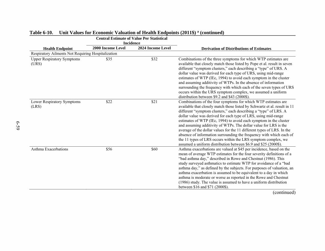
6-59
Table 6-10. Unit Values for Economic Valuation of Health Endpoints (2011$) a (continued)
Health Endpoint
Central Estimate of Value Per Statistical Incidence
Derivation of Distributions of Estimates 2000 Income Level 2024 Income Level Respiratory Ailments Not Requiring Hospitalization Upper Respiratory Symptoms (URS)
$35 $32 Combinations of the three symptoms for which WTP estimates are available that closely match those listed by Pope et al. result in seven different “symptom clusters,” each describing a “type” of URS. A dollar value was derived for each type of URS, using mid-range estimates of WTP (IEc, 1994) to avoid each symptom in the cluster and assuming additivity of WTPs. In the absence of information surrounding the frequency with which each of the seven types of URS occurs within the URS symptom complex, we assumed a uniform distribution between $9.2 and $43 (2000$).
Lower Respiratory Symptoms (LRS)
$22 $21 Combinations of the four symptoms for which WTP estimates are available that closely match those listed by Schwartz et al. result in 11 different “symptom clusters,” each describing a “type” of LRS. A dollar value was derived for each type of LRS, using mid-range estimates of WTP (IEc, 1994) to avoid each symptom in the cluster and assuming additivity of WTPs. The dollar value for LRS is the average of the dollar values for the 11 different types of LRS. In the absence of information surrounding the frequency with which each of the 11 types of LRS occurs within the LRS symptom complex, we assumed a uniform distribution between $6.9 and $25 (2000$).
Asthma Exacerbations $56 $60 Asthma exacerbations are valued at $45 per incidence, based on the mean of average WTP estimates for the four severity definitions of a “bad asthma day,” described in Rowe and Chestnut (1986). This study surveyed asthmatics to estimate WTP for avoidance of a “bad asthma day,” as defined by the subjects. For purposes of valuation, an asthma exacerbation is assumed to be equivalent to a day in which asthma is moderate or worse as reported in the Rowe and Chestnut (1986) study. The value is assumed to have a uniform distribution between $16 and $71 (2000$).
(continued)

6-60
Table 6-10. Unit Values for Economic Valuation of Health Endpoints (2011$) a (continued)
Health Endpoint Central Estimate of Value Per Statistical Incidence
Derivation of Distributions of Estimates 2000 Income Level 2024 Income Level Respiratory Ailments Not Requiring Hospitalization (continued) Acute Bronchitis $460 $500 Assumes a 6-day episode, with the distribution of the daily value
specified as uniform with the low and high values based on those recommended for related respiratory symptoms in Neumann et al. (1994). The low daily estimate of $10 is the sum of the mid-range values recommended by IEc (1994) for two symptoms believed to be associated with acute bronchitis: coughing and chest tightness. The high daily estimate was taken to be twice the value of a minor respiratory restricted-activity day, or $110 (2000$).
Work Loss Days (WLDs) Variable (U.S. median = $150)
Variable (U.S. median = $150)
No distribution available. Point estimate is based on county-specific median annual wages divided by 52 and then by 5—to get median daily wage. U.S. Year 2000 Census, compiled by Geolytics, Inc. (Geolytics, 2002)
School Loss Days $98 $98 No distribution available. Based on (1) the probability that, if a school child stays home from school, a parent will have to stay home from work to care for the child, and (2) the value of the parent’s lost productivity.
Minor Restricted Activity Days (MRADs)
$64 $68 Median WTP estimate to avoid one MRAD from Tolley et al. (1986). Distribution is assumed to be triangular with a minimum of $22 and a maximum of $83, with a most likely value of $52 (2000$). Range is based on assumption that value should exceed WTP for a single mild symptom (the highest estimate for a single symptom—for eye irritation—is $16) and be less than that for a WLD. The triangular distribution acknowledges that the actual value is likely to be closer to the point estimate than either extreme.
a All estimates are rounded to two significant digits. Unrounded estimates in 2000$ are available in the Appendix J of the BenMAP user manual (U.S. EPA, 2015). Income growth projections are only currently available in BenMAP through 2024, so both the 2025 and 2038 estimates use income growth through 2024 and are therefore likely underestimates. Currently, BenMAP does not have an inflation adjustment to 2011$. We ran BenMAP for a currency year of 2010$ and calculated the benefit-per-ton estimates in 2010$. We then adjusted the resulting benefit-per-ton estimates to 2011$ using the Consumer Price Index (CPI-U, all items). This approach slightly underestimates the inflation for medical index and wage index between 2010 and 2011, which affects COI estimates and wage-based estimates.

6-61
During this time, the Agency continued work to update its guidance on valuing mortality
risk reductions, including commissioning a report from meta-analytic experts to evaluate
methodological questions raised by the EPA and the SAB on combining estimates from the
various data sources. In addition, the Agency consulted several times with the SAB-EEAC on the
issue. With input from the meta-analytic experts, the SAB-EEAC advised the Agency to update
its guidance using specific, appropriate meta-analytic techniques to combine estimates from
unique data sources and different studies, including those using different methodologies (i.e.,
wage-risk and stated preference) (U.S. EPA-SAB, 2007).
Until updated guidance is available, the Agency determined that a single, peer-reviewed
estimate applied consistently best reflects the SAB-EEAC advice it has received. Therefore, the
Agency has decided to apply the VSL that was vetted and endorsed by the SAB in the Guidelines
for Preparing Economic Analyses (U.S. EPA, 2000)156 while the Agency continues its efforts to
update its guidance on this issue. This approach calculates a mean value across VSL estimates
derived from 26 labor market and contingent valuation studies published between 1974 and
1991. The mean VSL across these studies is $4.8 million (1990$) or $6.3 million (2000$).157 The
Agency is committed to using scientifically sound, appropriately reviewed evidence in valuing
mortality risk reductions and has made significant progress in responding to the SAB-EEAC’s
specific recommendations. In the process, the Agency has identified a number of important
issues to be considered in updating its mortality risk valuation estimates. These are detailed in a
white paper on “Valuing Mortality Risk Reductions in Environmental Policy,” which underwent
review by the SAB-EEAC. A meeting with the SAB on this paper was held on March 14, 2011
and formal recommendations were transmitted on July 29, 2011 (U.S. EPA-SAB, 2011). EPA is
taking SAB’s recommendations under advisement.
The economics literature concerning the appropriate method for valuing reductions in
premature mortality risk is still developing. The adoption of a value for the projected reduction in
the risk of premature mortality is the subject of continuing discussion within the economics and
156 In the updated Guidelines for Preparing Economic Analyses (U.S. EPA, 2010e), EPA retained the VSL endorsed
by the SAB with the understanding that further updates to the mortality risk valuation guidance would be forthcoming in the near future.
157 In this analysis, we adjust the VSL to account for a different currency year (2011$) and to account for income growth to 2024. After applying these adjustments to the $6.3 million value, the VSL is $10 million.

6-62
public policy analysis communities. The EPA strives to use the best economic science in its
analyses. Given the mixed theoretical finding and empirical evidence regarding adjustments to
VSL for risk and population characteristics (e.g., Smith et al., 2004; Alberini et al., 2004; Aldy
and Viscusi, 2008), we use a single VSL for all reductions in mortality risk.
Although there are several differences between the studies the EPA uses to derive a VSL
estimate and the ozone and PM2.5 air pollution context addressed here, those differences in the
affected populations and the nature of the risks imply both upward and downward adjustments.
Table 6-11 lists some of these differences and the expected effect on the VSL estimate for air
pollution-related mortality. In the absence of a comprehensive and balanced set of adjustment
factors, the EPA believes it is reasonable to continue to use the $4.8 million (1990$) value
adjusted for inflation and income growth over time while acknowledging the significant
limitations and uncertainties in the available literature.
Table 6-11. Influence of Applied VSL Attributes on the Size of the Economic Benefits of Reductions in the Risk of Premature Mortality (U.S. EPA, 2006a)
Attribute Expected Direction of Bias Age Uncertain, perhaps overestimate Life Expectancy/Health Status Uncertain, perhaps overestimate Attitudes Toward Risk Underestimate Income Uncertain Voluntary vs. Involuntary Uncertain, perhaps underestimate Catastrophic vs. Protracted Death Uncertain, perhaps underestimate
The SAB-EEAC has reviewed many potential VSL adjustments and the state of the
economics literature. The SAB-EEAC advised the EPA to “continue to use a wage-risk-based
VSL as its primary estimate, including appropriate quantitative uncertainty analyses to reflect the
uncertainty of these estimates,” and that “the only risk characteristic for which adjustments to the
VSL can be made is the timing of the risk” (U.S. EPA-SAB, 2000). In developing our core
estimate of the benefits of premature mortality reductions, we followed this advice.
For PM2.5-related premature mortality, we assume that there is a “cessation” lag between
exposures and the total realization of changes in health effects. For PM2.5, we assumed that some
of the incidences of premature mortality related to PM2.5 exposures occur in a distributed fashion
over the 20 years following exposure and discounted over the period between exposure and
6-63
premature mortality. Although the structure of the lag is uncertain, the EPA follows the advice of
the SAB-HES to assume a segmented lag structure characterized by 30 percent of mortality
reductions in the first year, 50 percent over years 2 to 5, and 20 percent over the years 6 to 20
after the reduction in PM2.5 (U.S. EPA-SAB, 2004c). To take this into account in the valuation of
reductions in premature mortality, we discount the value of premature mortality occurring in
future years using rates of 3 percent and 7 percent.158 Changes in the cessation lag assumptions
do not change the total estimated premature mortality but rather the timing of those deaths. As
such, the monetized PM2.5 co-benefits using a 7 percent discount rate are only approximately 10
percent less than the monetized benefits using a 3 percent discount rate. Further discussion of
this topic appears in the EPA’s Guidelines for Preparing Economic Analyses (U.S. EPA, 2010e).
For ozone, we acknowledge substantial uncertainty associated with specifying the lag for
long-term respiratory mortality. As stated earlier, it is this uncertainty related to specifying a lag
structure that prevented us monetizing these benefits. In the quantitative uncertainty analysis, we
include both an assumption of zero lag and the PM lag structure (i.e., the SAB 20-year
segmented lag). Inclusion of the zero lag reflects consideration of the possibility that the long-
term respiratory mortality estimate primarily captures an accumulation of short-term mortality
effects across the ozone season.159 The use of the 20-year segmented lag reflects consideration of
advice provided by the SAB-HES (U.S. EPA-SAB, 2010a), where they state that, “[i]f
Alternative estimates are derived using cohort mortality evidence, there is no evidence in the
literature to support a different cessation lag between ozone and particulate matter. The HES
therefore recommends using the same cessation lag structure and assumptions as for particulate
matter when utilizing cohort mortality evidence for ozone.” Monetized benefit estimates
158 The choice of a discount rate, and its associated conceptual basis, is a topic of ongoing discussion within the
federal government. To comply with OMB Circular A-4, EPA provides monetized benefits using discount rates of 3% and 7% (OMB, 2003). A 3% discount reflects reliance on a “social rate of time preference” discounting concept. A 7% rate is consistent with an “opportunity cost of capital” concept to reflect the time value of resources directed to meet regulatory requirements.
159 The ozone HREA noted,: “The effect estimates used in modeling long-term O3-attributable mortality, utilize a seasonal average of peak (1-hr maximum) measurements. These long-term exposure metrics can be viewed as long-term exposures to daily peak O3 over the warmer months, as compared with annual average levels such as are used in long-term PM exposure calculations. This increases the need for care in interpreting these long-term O3-attributable mortality estimates together with the short-term O3-attributable mortality estimates, in order to avoid double counting.” (U.S. EPA, 2014b).

6-64
generated using both lag assumptions are presented as quantitative uncertainty analyses (see
section 6.7.3.1).
Uncertainties Specific to Premature Mortality Valuation. The economic benefits
associated with reductions in the risk of premature mortality are the largest category of
monetized benefits in this RIA. In addition, in prior analyses, the EPA identified valuation of
mortality-related benefits as the largest contributor to the range of uncertainty in monetized
benefits (Mansfield et al., 2009).160 Because of the uncertainty in estimates of the value of
reducing premature mortality risk, it is important to adequately characterize and understand the
various types of economic approaches available for valuing reductions in mortality risk. Such an
assessment also requires an understanding of how alternative valuation approaches reflect that
some individuals may be more susceptible to air pollution-induced mortality or reflect
differences in the nature of the risk presented by air pollution relative to the risks studied in the
relevant economics literature.
The health science literature on air pollution indicates that several human characteristics
affect the degree to which mortality risk affects an individual. For example, some age groups
appear to be more susceptible to air pollution than others (e.g., the elderly and children). Health
status prior to exposure also affects susceptibility. An ideal benefits estimate of mortality risk
reduction would reflect these human characteristics, in addition to an individual’s WTP to
improve one’s own chances of survival along with WTP to improve other individuals’ survival
rates. The ideal measure would also take into account the specific nature of the risk reduction
commodity that is provided to individuals, as well as the context in which risk is reduced. To
measure this value, it is important to assess how reductions in air pollution reduce the risk of
dying from the time that reductions take effect onward and how individuals value these changes.
Each individual’s survival curve, or the probability of surviving beyond a given age, should shift
as a result of an environmental quality improvement. For example, changing the current
probability of survival for an individual also shifts future probabilities of that individual’s
survival. This probability shift will differ across individuals because survival curves depend on
160 This conclusion was based on an assessment of uncertainty based on statistical error in epidemiological effect
estimates and economic valuation estimates. Additional sources of model error such as those examined in the PM2.5 mortality expert elicitation (Roman et al., 2008) may result in different conclusions about the relative contribution of sources of uncertainty.

6-65
such characteristics as age, health state, and the current age to which the individual is likely to
survive.
Although a survival curve approach provides a theoretically preferred method for valuing
the benefits of reduced risk of premature mortality associated with reducing air pollution, the
approach requires a great deal of data to implement. The economic valuation literature does not
yet include good estimates of the value of this risk reduction commodity. As a result, in this
analysis we value reductions in premature mortality risk using the VSL approach.
Other uncertainties specific to premature mortality valuation include the following:
Across-study variation: There is considerable uncertainty as to whether the available literature on VSL provides adequate estimates of the VSL for risk reductions from air pollution reduction. Although there is considerable variation in the analytical designs and data used in the existing literature, the majority of the studies involve the value of risks to a middle-aged working population. Most of the studies examine differences in wages of risky occupations, using a hedonic wage approach. Certain characteristics of both the population affected and the mortality risk facing that population are believed to affect the average WTP to reduce the risk. The appropriateness of a distribution of WTP based on the current VSL literature for valuing the mortality-related benefits of reductions in air pollution concentrations therefore depends not only on the quality of the studies (i.e., how well they measure what they are trying to measure), but also on the extent to which the risks being valued are similar and the extent to which the subjects in the studies are similar to the population affected by changes in pollution concentrations.
Level of risk reduction: The transferability of estimates of the VSL from the wage-risk studies to the context of this analysis rests on the assumption that, within a reasonable range, WTP for reductions in mortality risk is linear in risk reduction. For example, suppose a study provides a result that the average WTP for a reduction in mortality risk of 1/100,000 is $50, but that the actual mortality risk reduction resulting from a given pollutant reduction is 1/10,000. If WTP for reductions in mortality risk is linear in risk reduction, then a WTP of $50 for a reduction of 1/100,000 implies a WTP of $500 for a risk reduction of 1/10,000 (which is 10 times the risk reduction valued in the study). Under the assumption of linearity, the estimate of the VSL does not depend on the particular amount of risk reduction being valued. This assumption has been shown to be reasonable provided the change in the risk being valued is within the range of risks evaluated in the underlying studies (Rowlatt et al., 1998).
Voluntariness of risks evaluated: Although job-related mortality risks may differ in several ways from air pollution-related mortality risks, the most important difference may be that job-related risks are incurred voluntarily, or generally assumed to be, whereas air pollution-related risks are incurred involuntarily. Some evidence suggests that people will pay more to reduce involuntarily incurred risks than risks incurred voluntarily (e.g.,
6-66
Lichtenstein and Slovic, 2006). If this is the case, WTP estimates based on wage-risk studies may understate WTP to reduce involuntarily incurred air pollution-related mortality risks.
Sudden versus protracted death: A final important difference related to the nature of the risk may be that some workplace mortality risks tend to involve sudden, traumatic events, whereas air pollution-related risks tend to involve longer periods of disease and suffering prior to death. Some evidence suggests that WTP to avoid a risk of a protracted death involving prolonged suffering and loss of dignity and personal control is greater than the WTP to avoid a risk (of identical magnitude) of sudden death (e.g., Tsuge et al., 2005; Alberini and Scasny, 2011). To the extent that the mortality risks addressed in this assessment are associated with longer periods of illness or greater pain and suffering than are the risks addressed in the valuation literature, the WTP measurements employed in the present analysis would reflect a downward bias.
Self-selection and skill in avoiding risk: Recent research (Shogren and Stamland, 2002) suggests that VSL estimates based on hedonic wage studies may overstate the average value of a risk reduction. This is because the risk-wage trade-off revealed in hedonic studies reflects the preferences of the marginal worker (i.e., that worker who demands the highest compensation for his risk reduction for a given job). This worker must have either a higher workplace risk than the average worker in a given occupation, a lower risk tolerance than the average worker in that occupation, or both. Conversely, the marginal worker should have a higher risk tolerance than workers employed in less-risky sectors. However, the risk estimate used in hedonic studies is generally based on average risk, so the VSL may be biased, in an ambiguous direction, because the wage differential and risk measures do not match.
Baseline risk and age: Recent research (Smith, Pattanayak, and Van Houtven, 2006) finds that because individuals reevaluate their baseline risk of death as they age, the marginal value of risk reductions does not decline with age as predicted by some lifetime consumption models. This research supports findings in recent stated preference studies that suggest only small reductions in the value of mortality risk reductions with increasing age (e.g., Alberini et al., 2004).
6.6.4.2 Hospital Admissions and Emergency Department Valuation
In the absence of estimates of societal WTP to avoid hospital visits/admissions for
specific illnesses, we derive COI estimates for use in the benefits analysis. The International
Classification of Diseases (ICD) (WHO, 1977) code-specific COI estimates used in this analysis
consist of estimated hospital charges and the estimated opportunity cost of time spent in the
hospital (based on the average length of a hospital stay for the illness). We based all estimates of
hospital charges and length of stays on statistics provided by the Agency for Healthcare Research
and Quality’s Healthcare Utilization Project National Inpatient Sample (NIS) database (AHRQ,

6-67
2007). We estimated the opportunity cost of a day spent in the hospital as the value of the lost
daily wage, regardless of whether the hospitalized individual is in the workforce. To estimate the
lost daily wage, we divided the median weekly wage reported by the 2007 American Community
Survey (ACS) by five and deflated the result to the correct currency year using the CPI-U “all
items” (U.S. EPA, 2015). The resulting national average lost daily wage is $150 (2011$). The
total cost-of-illness estimate for an ICD code-specific hospital stay lasting n days, then, was the
mean hospital charge plus daily lost wage multiplied by n. In general, the mean length of stay
has decreased since the 2000 database used in the previous version of BenMAP, while the mean
hospital charge has increased. We provide the rounded unit values in 2011$ for the COI
functions used in this analysis in Table 6-12.
Table 6-12. Unit Values for Hospital Admissions a
End Point ICD Codes Age Range Mean Hospital
Charge (2011$)
Mean Length of
Stay (days)
Total Cost of Illness (unit
value in 2011$) min. max.
HA, Chronic Lung Disease 490–496 18 64 $20,000 3.9 $22,000 HA, Asthma 493 0 64 $15,000 3.0 $16,000 HA, All Cardiovascular 390–429 18 64 $41,000 4.1 $44,000 HA, All Cardiovascular 390–429 65 99 $38,000 4.9 $42,000 HA, All Respiratory 460–519 65 99 $32,000 6.1 $37,000
a All estimates rounded to two significant digits. Unrounded estimates in 2000$ are available in Appendix J of the BenMAP user manual (U.S. EPA, 2015).
To value asthma emergency department visits, we used a simple average of two estimates
from the health economics literature. The first estimate comes from Smith et al. (1997), who
reported approximately 1.2 million asthma-related emergency department visits in 1987, at a
total cost of $186 million (1987$). The average cost per visit that year was $155; in 2011$, that
cost is $480 (using the CPI-U for medical care to adjust to 2011$). The second estimate comes
from Stanford et al. (1999), who reported the cost of an average asthma-related emergency
department visit based on 1996–1997 data at $400 (using the CPI-U for medical care to adjust to
2011$). A simple average of the two estimates yields a unit value of $440 (2011$).
6.6.4.3 Nonfatal Myocardial Infarctions Valuation
We were not able to identify a suitable WTP value for reductions in the risk of nonfatal
heart attacks. Instead, we use a COI unit value with two components: the direct medical costs
and the opportunity cost (lost earnings) associated with the illness event. Because the costs

6-68
associated with a myocardial infarction extend beyond the initial event itself, we consider costs
incurred over several years. Using age-specific annual lost earnings estimated by Cropper and
Krupnick (1990) and a 3% discount rate, we estimated a rounded present discounted value in lost
earnings (in 2000$) over 5 years due to a myocardial infarction of $8,800 for someone between
the ages of 25 and 44, $13,000 for someone between the ages of 45 and 54, and $75,000 for
someone between the ages of 55 and 65. The rounded corresponding age-specific estimates of
lost earnings (in 2000$) using a 7% discount rate are $7,900, $12,000, and $67,000, respectively.
Cropper and Krupnick (1990) do not provide lost earnings estimates for populations under 25 or
over 65. As such, we do not include lost earnings in the cost estimates for these age groups.
We found three possible sources in the literature of estimates of the direct medical costs
of myocardial infarction, which provide significantly different values (see Table 6-13):
Wittels et al. (1990) estimated expected total medical costs of myocardial infarction over 5 years to be $51,000 (rounded in 1986$) for people who were admitted to the hospital and survived hospitalization. (There does not appear to be any discounting used.) This estimated cost is based on a medical cost model, which incorporated therapeutic options, projected outcomes, and prices (using “knowledgeable cardiologists” as consultants). The model used medical data and medical decision algorithms to estimate the probabilities of certain events and/or medical procedures being used. The authors note that the average length of hospitalization for acute myocardial infarction has decreased over time (from an average of 12.9 days in 1980 to an average of 11 days in 1983). Wittels et al. used 10 days as the average in their study. It is unclear how much further the length of stay for myocardial infarction may have decreased from 1983 to the present. The average length of stay for ICD code 410 (myocardial infarction) in the year-2000 Agency for Healthcare Research and Quality (AHRQ) HCUP database is 5.5 days (AHRQ, 2000). However, this may include patients who died in the hospital (not included among our nonfatal myocardial infarction cases), and as a result whose length of stay was substantially shorter.
Eisenstein et al. (2001) estimated 10-year costs of $45,000 in rounded 1997$ (using a 3% discount rate) for myocardial infarction patients, using statistical prediction (regression) models to estimate inpatient costs. Only inpatient costs (physician fees and hospital costs) were included.

6-69
Table 6-13. Alternative Direct Medical Cost of Illness Estimates for Nonfatal Heart Attacks a
Study Direct Medical Costs (2011$) Over an x-Year Period, for x = Wittels et al. (1990) $170,000 b 5 Russell et al. (1998) $34,000 c 5 Average (5-year) costs $100,000 5 Eisenstein et al. (2001) $76,000 c 10
a All estimates rounded to two significant digits. Unrounded estimates in 2000$ are available in appendix J of the BenMAP user manual (U.S. EPA, 2015). b Wittels et al. (1990) did not appear to discount costs incurred in future years. c Using a 3% discount rate. Discounted values as reported in the study.
As noted above, the estimates from these three studies are substantially different, and we
have not adequately resolved the sources of differences in the estimates. Because the wage-
related opportunity cost estimates from Cropper and Krupnick (1990) cover a 5-year period, we
used estimates for medical costs that similarly cover a 5-year period (i.e., estimates from Wittels
et al. (1990) and Russell et al. (1998). We used a simple average of the two 5-year estimates, or
rounded to $85,000, and added it to the 5-year opportunity cost estimate. The resulting estimates
are given in Table 6-14.
Table 6-14. Estimated Costs Over a 5-Year Period of a Nonfatal Myocardial Infarction (in 2011$) a
Age Group Opportunity Cost Medical Cost b Total Cost 0–24 $0 $100,000 $100,000 25–44 $12,000 c $100,000 $110,000 45–54 $18,000 c $100,000 $120,000 55–65 $100,000 c $100,000 $210,000 > 65 $0 $100,000 $100,000
a All estimates rounded to two significant digits, so estimates may not sum across columns. Unrounded estimates in 2000$ are available in appendix J of the BenMAP user manual (U.S. EPA, 2015). b An average of the 5-year costs estimated by Wittels et al. (1990) and Russell et al. (1998). c From Cropper and Krupnick (1990), using a 3% discount rate for illustration. 6.6.4.4 Valuation of Acute Health Events
Asthma Exacerbation Valuation. Several respiratory symptoms in asthmatics or
characterizations of an asthma episode have been associated with exposure to air pollutants. All
of these can generally be taken as indications of an asthma exacerbation when they occur in an
asthmatic. Therefore, we apply the same set of unit values for all of the variations of “asthma
exacerbation”. Specifically, we use a unit value based on the mean WTP estimates for a “bad
asthma day,” described in Rowe and Chestnut (1986). This study surveyed asthmatics to estimate
WTP for avoidance of a “bad asthma day,” as defined by the subjects.

6-70
Minor Restricted Activity Days Valuation. No studies are reported to have estimated
WTP to avoid a minor restricted activity day. However, Neumann et al. (1994) derived an
estimate of willingness to pay to avoid a minor respiratory restricted activity day, using estimates
from Tolley et al. (1986) of WTP for avoiding a combination of coughing, throat congestion and
sinusitis. This estimate of WTP to avoid a minor respiratory restricted activity day is $38
(1990$), or about $71 (2011$). Although Ostro and Rothschild (1989) statistically linked ozone
and minor restricted activity days, it is likely that most MRADs associated with ozone and PM2.5
exposure are, in fact, minor respiratory restricted activity days. For the purpose of valuing this
health endpoint, we used the estimate of mean WTP to avoid a minor respiratory restricted
activity day.
School Loss Days Valuation. To value a school absence, we: (1) estimated the
probability that if a school child stays home from school, a parent will have to stay home from
work to care for the child; and (2) valued the lost productivity at the parent’s wage. To do this,
we estimated the number of families with school-age children in which both parents work, and
we valued a school-loss day as the probability that such a day also would result in a work-loss
day. We calculated this value by multiplying the proportion of households with school-age
children by a measure of lost wages.
We used this method in the absence of a preferable WTP method. However, this
approach suffers from several uncertainties. First, it omits willingness to pay to avoid the
symptoms/illness that resulted in the school absence; second, it effectively gives zero value to
school absences that do not result in work-loss days; and third, it uses conservative assumptions
about the wages of the parent staying home with the child. Finally, this method assumes that
parents are unable to work from home. If this is not a valid assumption, then there would be no
lost wages.
For this valuation approach, we assumed that in a household with two working parents,
the female parent will stay home with a sick child. From the Statistical Abstract of the United
States (U.S. Census Bureau, 2001), we obtained: (1) the numbers of single, married and “other”
(widowed, divorced or separated) working women with children; and (2) the rates of
participation in the workforce of single, married and “other” women with children. From these
two sets of statistics, we calculated a weighted average participation rate of 72.85 percent. Our

6-71
estimate of daily lost wage (wages lost if a mother must stay at home with a sick child) is based
on the year 2000 median weekly wage among women ages 25 and older (U.S. Census Bureau,
2001). This median weekly wage is $551 (2000$). Dividing by five gives an estimated median
daily wage of $103 (2000$). To estimate the expected lost wages on a day when a mother has to
stay home with a school-age child, we first estimated the probability that the mother is in the
workforce then multiplied that estimate by the daily wage she would lose by missing a workday:
72.85 percent times $103, for a total loss of $75 (2000$). This valuation approach is similar to
that used by Hall et al. (2003).
Work Loss Days Valuation. Work loss days are valued at a day’s wage. BenMAP-CE
calculates county-specific median daily wages from county-specific annual wages (by dividing
the annual wage by 52 weeks multiplied by 5 work days per week), on the theory that a worker’s
vacation days are valued at the same daily rate as work days.
Upper and Lower Respiratory Symptoms Valuation. Lower and upper respiratory
symptoms are each considered a complex of symptoms. A dollar value was derived for clusters
of these symptoms that most closely match the studies used to calculate incidence (Schwartz and
Neas, 2000; Pope et al., 1991) based on mid-range estimates from each cluster (IEc, 1994).
6.6.4.5 Growth in WTP Reflecting National Income Growth over Time
Our analysis accounts for expected growth in real income over time. This is a distinct
concept from inflation and currency year. Economic theory argues that WTP for most goods
(such as environmental protection) will increase if real incomes increase. There is substantial
empirical evidence that the income elasticity161 of WTP for health risk reductions is positive,
although there is uncertainty about its exact value. Thus, as real income increases, the WTP for
environmental improvements also increases. Although many analyses assume that the income
elasticity of WTP is unit elastic (i.e., a 10% higher real income level implies a 10% higher WTP
to reduce risk changes), empirical evidence suggests that income elasticity is substantially less
161 Income elasticity is a common economic measure equal to the percentage change in WTP for a 1 percent change
in income.
6-72
than one and thus relatively inelastic. As real income rises, the WTP value also rises but at a
slower rate than real income.
The effects of real income changes on WTP estimates can influence benefits estimates in
two different ways: through real (national average) income growth between the year a WTP
study was conducted and the year for which benefits are estimated, and through differences in
income between study populations and the affected populations at a particular time. The SAB-
EEAC advised the EPA to adjust WTP for increases in real income over time but not to adjust
WTP to account for cross-sectional income differences “because of the sensitivity of making
such distinctions, and because of insufficient evidence available at present” (U.S. EPA-SAB,
2000). An advisory by another committee associated with the SAB, the Advisory Council on
Clean Air Compliance Analysis (SAB-Council), has provided conflicting advice. While agreeing
with “the general principle that the willingness to pay to reduce mortality risks is likely to
increase with growth in real income” and that “[t]he same increase should be assumed for the
WTP for serious nonfatal health effects,” they note that “given the limitations and uncertainties
in the available empirical evidence, the Council does not support the use of the proposed
adjustments for aggregate income growth as part of the primary analysis” (U.S. EPA-SAB,
2004b). More recently, in response to questions related to the adjustment for income growth over
time, the SAB-EEAC noted that “EPA should adjust for changes in income in evaluating benefits
of risk reduction” (U.S. EPA-SAB, 2011). Until these conflicting advisories can be reconciled,
the EPA will continue to adjust valuation estimates to reflect income growth using the methods
described below, while providing quantitative uncertainty analyses for alternative income growth
adjustment factors.
Based on a review of the available income elasticity literature, we adjusted the valuation
of human health benefits upward to account for projected growth in real U.S. income. Faced with
a dearth of estimates of income elasticities derived from time-series studies, we applied estimates
derived from cross-sectional studies in our analysis. Details of the procedure can be found in
Kleckner and Neumann (1999). We note that the literature has evolved since the publication of
this memo and that an array of newer studies identifying potentially suitable income elasticity
estimates are available (IEc, 2012). The EPA anticipates seeking a peer review in the near future
of these studies and its approach to adjusting WTP estimates to account for changes in personal
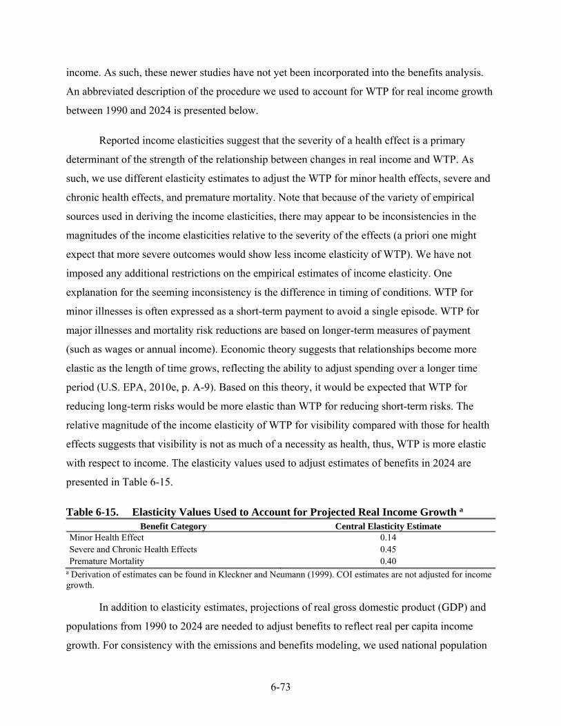
6-73
income. As such, these newer studies have not yet been incorporated into the benefits analysis.
An abbreviated description of the procedure we used to account for WTP for real income growth
between 1990 and 2024 is presented below.
Reported income elasticities suggest that the severity of a health effect is a primary
determinant of the strength of the relationship between changes in real income and WTP. As
such, we use different elasticity estimates to adjust the WTP for minor health effects, severe and
chronic health effects, and premature mortality. Note that because of the variety of empirical
sources used in deriving the income elasticities, there may appear to be inconsistencies in the
magnitudes of the income elasticities relative to the severity of the effects (a priori one might
expect that more severe outcomes would show less income elasticity of WTP). We have not
imposed any additional restrictions on the empirical estimates of income elasticity. One
explanation for the seeming inconsistency is the difference in timing of conditions. WTP for
minor illnesses is often expressed as a short-term payment to avoid a single episode. WTP for
major illnesses and mortality risk reductions are based on longer-term measures of payment
(such as wages or annual income). Economic theory suggests that relationships become more
elastic as the length of time grows, reflecting the ability to adjust spending over a longer time
period (U.S. EPA, 2010e, p. A-9). Based on this theory, it would be expected that WTP for
reducing long-term risks would be more elastic than WTP for reducing short-term risks. The
relative magnitude of the income elasticity of WTP for visibility compared with those for health
effects suggests that visibility is not as much of a necessity as health, thus, WTP is more elastic
with respect to income. The elasticity values used to adjust estimates of benefits in 2024 are
presented in Table 6-15.
Table 6-15. Elasticity Values Used to Account for Projected Real Income Growth a Benefit Category Central Elasticity Estimate
Minor Health Effect 0.14 Severe and Chronic Health Effects 0.45 Premature Mortality 0.40
a Derivation of estimates can be found in Kleckner and Neumann (1999). COI estimates are not adjusted for income growth.
In addition to elasticity estimates, projections of real gross domestic product (GDP) and
populations from 1990 to 2024 are needed to adjust benefits to reflect real per capita income
growth. For consistency with the emissions and benefits modeling, we used national population

6-74
estimates for the years 1990 to 1999 based on U.S. Census Bureau estimates (Hollman, Mulder,
and Kallan, 2000). These population estimates are based on application of a cohort-component
model applied to 1990 U.S. Census data projections (U.S. Bureau of Census, 2000). For the
years between 2000 and 2024, we applied growth rates based on the U.S. Census Bureau
projections to the U.S. Census estimate of national population in 2000. We used projections of
real GDP provided in Kleckner and Neumann (1999) for the years 1990 to 2010.162 We used
projections of real GDP (in chained 1996 dollars) provided by Standard and Poor’s (2000) for
the years 2010 to 2024.163
Using the method outlined in Kleckner and Neumann (1999) and the population and
income data described above, we calculated WTP adjustment factors for each of the elasticity
estimates listed in Table 6-16. Benefits for each of the categories (minor health effects, severe
and chronic health effects, premature mortality, and visibility) are adjusted by multiplying the
unadjusted benefits by the appropriate adjustment factor. For premature mortality, we applied the
income adjustment factor specific to the analysis year, but we do not adjust for income growth
over the 20-year cessation lag. Our approach could underestimate the benefits for the later years
of the lag.
There is some uncertainty regarding the total costs of illness in the future. Specifically,
the nature of medical treatment is changing, including a shift towards more outpatient treatment.
Although we adjust the COI estimates for inflation, we do not have data to project COI estimates
for the cost of treatment in the future or income growth over time, which leads to an inherent
though unavoidable inconsistency between COI- and WTP-based estimates. This approach may
under predict benefits in future years because it is likely that increases in real U.S. income would
also result in increased COI (due, for example, to increases in wages paid to medical workers)
and increased cost of work loss days and lost worker productivity (reflecting that if worker
162 U.S. Bureau of Economic Analysis, Table 2A—Real Gross Domestic Product (1997) and U.S. Bureau of
Economic Analysis, The Economic and Budget Outlook: An Update, Table 4—Economic Projections for Calendar Years 1997 Through 2007 (1997). Note that projections for 2007 to 2010 are based on average GDP growth rates between 1999 and 2007.
163 In previous analyses, we used the Standard and Poor’s projections of GDP directly. This led to an apparent discontinuity in the adjustment factors between 2010 and 2011. We refined the method by applying the relative growth rates for GDP derived from the Standard and Poor’s projections to the 2010 projected GDP based on the Bureau of Economic Analysis projections.

6-75
incomes are higher, the losses resulting from reduced worker production would also be higher).
In addition, cost-of-illness estimates do not include sequelae costs or pain and suffering, the
value of which would likely increase in the future. To the extent that costs would be expected to
increase over time, this increase may be partially offset by advancement in medical technology
that improves the effectiveness of treatment at lower costs. For these reasons, we believe that the
cost-of-illness estimates in this RIA may underestimate (on net) the total economic value of
avoided health impacts.
Table 6-16. Adjustment Factors Used to Account for Projected Real Income Growth a Benefit Category 2024 Minor Health Effect 1.07 Severe and Chronic Health Effects 1.22 Premature Mortality 1.20
a Based on elasticity values reported in Table 6-15, U.S. Census population projections, and projections of real GDP per capita. 6.6.5 Benefit per Ton Estimates Used in Modeling PM2.5-Related Co-benefits
This section presents the benefit-per-ton estimates (dimensioned by mortality study and
simulation year) used as inputs in generating PM2.5 co-benefits estimates including (Table 6-17).
Benefit-per-ton estimates were generated for each of the long-term exposure-related mortality
studies used in generating core benefits estimates for this RIA including Krewski et al. (2009)
and Lepeule et al. (2012) (see section 6.6.3.3). Estimates were available for 2025 and 2030, with
those being used to model co-benefits for the 2025 scenario and post-2025 scenario, respectively.
For additional detail on the approach used to generate PM2.5 co-benefits estimates and the role
played by these two types of inputs, see Section 6.4.4.164
164 Sector-level NOx reductions (for each alternative standard level) were generated using methods described in
Chapter 4, section 4.2 and 4.3. As noted in section 5.4.4, NOx emissions reductions associated with alternative standard levels considered for this NAAQS review involved seven of the 17 sectors for which we had benefit-per ton values and consequently, the co-benefits PM2.5 estimates are based on simulated benefits for those seven sectors.

6-76
Table 6-17. Summary of PM2.5 Benefit-per-ton Estimates a
a Benefit-per-ton estimates reflect application of the 20-year segmented lag at either a 3% or 7% discount rate. In addition, separate sets of benefit-per-ton estimates were generate for 2025 and 2030, reflecting application of appropriate projected demographic and baseline incidence data. b Benefit-per-ton estimates for the non-specified source category were generated as a weighted average of values for the 17 source categories, with weighting based on sector-specific NOx emissions for 2005 obtained from Fann et al. (2012b).
air,
locamotive
and
marine
cement
kilns
coke
ovens
EGU
point
electric
arc
furnaces
ferro
alloys
integrated
iron and
steel
iron and
steel
non‐EGU
point
other
non‐
point
other nonroad onroad
pulp and
paper refineries
residenti
al wood
taconite
mining
ocean
going
vessels
Non‐
specified
source b
2025 at 7% social discount
Krewski et al., 2009 $7,200 $5,700 $10,000 $5,200 $9,600 $4,400 $13,000 $17,000 $6,300 $7,900 $7,000 $7,600 $3,700 $6,900 $14,000 $6,000 $2,000 $6,400
Lepeule et al., 2012 $16,000 $13,000 $24,000 $12,000 $22,000 $9,800 $30,000 $38,000 $14,000 $18,000 $16,000 $17,000 $8,500 $16,000 $31,000 $14,000 $4,600 $15,000
2025 at 3% social discount
Krewski et al., 2009 $8,000 $6,300 $12,000 $5,800 $11,000 $4,800 $15,000 $19,000 $7,000 $8,700 $7,700 $8,400 $4,200 $7,700 $15,000 $6,600 $2,300 $7,100
Lepeule et al., 2012 $18,000 $14,000 $26,000 $13,000 $24,000 $11,000 $34,000 $42,000 $16,000 $20,000 $17,000 $19,000 $9,400 $17,000 $34,000 $15,000 $5,100 $16,000
2030 at 7% social discount
Krewski et al., 2009 $7,800 $6,100 $11,000 $5,600 $10,000 $4,600 $14,000 $18,000 $6,800 $8,500 $7,600 $8,200 $4,000 $7,500 $15,000 $6,400 $2,300 $6,900
Lepeule et al., 2012 $18,000 $14,000 $25,000 $13,000 $23,000 $10,000 $32,000 $41,000 $15,000 $19,000 $17,000 $19,000 $9,100 $17,000 $33,000 $14,000 $5,100 $16,000
2030 at 3% social discount
Krewski et al., 2009 $8,700 $6,800 $12,000 $6,200 $11,000 $5,100 $16,000 $20,000 $7,600 $9,400 $8,400 $9,100 $4,500 $8,300 $16,000 $7,100 $2,500 $7,700Lepeule et al., 2012 $20,000 $15,000 $28,000 $14,000 $26,000 $12,000 $36,000 $46,000 $17,000 $21,000 $19,000 $21,000 $10,000 $19,000 $37,000 $16,000 $5,600 $17,000
Long‐term mortality
study
Emissions sector
6-77
6.7 Benefits Results
We estimated the benefits of attaining the revised and alternative ozone standard levels
across the U.S. in 2025 except California. We estimated the benefits of attaining these standard
levels in California in 2038. We report the 2025 and 2038 estimates separately because deriving
a summed estimate would require us to calculate the Present Value (PV) of the stream of benefits
occurring between those two years, which is not possible with the available data. Additional
analyses (section 6.7.3) inform the interpretation of these core analyses.
Applying the impact and valuation functions described above to the estimated changes in
ozone concentrations yields estimates of the changes in physical damages (e.g., premature
deaths, cases of hospital admissions) and the associated monetary values for those changes. Not
all known ozone and PM health effects could be quantified or monetized, and the monetized
value of these unquantified effects is represented by adding an unknown “B” to the aggregate
total. Values are rounded to two significant figures and so totals may not sum across columns or
rows.
6.7.1 Benefits of Attaining a Revised Ozone Standard in 2025
This section presents the avoided health impacts and monetized benefits of attaining a
more stringent ozone standard in 2025. Table 6-18 shows the population-weighted air quality
change for the revised and alternative standard levels averaged across the continental U.S. Table
6-19 summarizes the tons of NOx emissions required to simulate attainment of the revised and
alternative standard levels (further differentiated by geographic region including east, west and
California). Tables 6-20 through 6-25 present the benefits results for the standard levels
analyzed. Table 6-25 summarizes total benefits by geographic region (including east, west minus
California, and California).
In addition, Figure 6-4 presents a quantitative uncertainty analysis for short-term ozone-
related benefits using additional C-R functions for premature mortality, and Figure 6-5 presents a
quantitative uncertainty analysis for PM2.5-related co-benefits using additional C-R functions for
premature mortality. See sections 6.6.3.2 and 6.6.3.3, respectively for additional discussion of
the alternative effect estimates used in each quantitative uncertainty analysis.
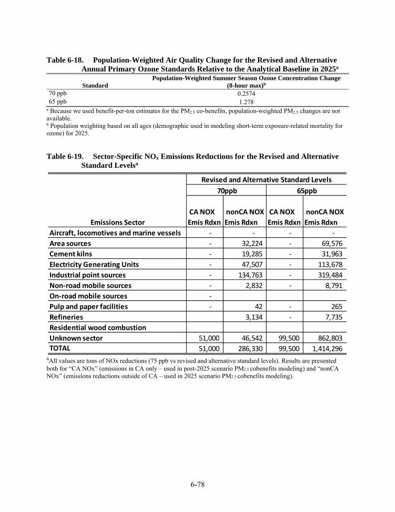
6-78
Table 6-18. Population-Weighted Air Quality Change for the Revised and Alternative
Annual Primary Ozone Standards Relative to the Analytical Baseline in 2025a
Standard Population-Weighted Summer Season Ozone Concentration Change
(8-hour max)b 70 ppb 0.2574 65 ppb 1.278
a Because we used benefit-per-ton estimates for the PM2.5 co-benefits, population-weighted PM2.5 changes are not available. b Population weighting based on all ages (demographic used in modeling short-term exposure-related mortality for ozone) for 2025. Table 6-19. Sector-Specific NOx Emissions Reductions for the Revised and Alternative
Standard Levelsa
aAll values are tons of NOx reductions (75 ppb vs revised and alternative standard levels). Results are presented both for “CA NOx” (emissions in CA only – used in post-2025 scenario PM2.5 cobenefits modeling) and “nonCA NOx” (emissions reductions outside of CA – used in 2025 scenario PM2.5 cobenefits modeling).
CA NOX
Emis Rdxn
nonCA NOX
Emis Rdxn
CA NOX
Emis Rdxn
nonCA NOX
Emis Rdxn
Aircraft, locomotives and marine vessels ‐ ‐ ‐ ‐
Area sources ‐ 32,224 ‐ 69,576
Cement kilns ‐ 19,285 ‐ 31,963
Electricity Generating Units ‐ 47,507 ‐ 113,678
Industrial point sources ‐ 134,763 ‐ 319,484
Non‐road mobile sources ‐ 2,832 ‐ 8,791
On‐road mobile sources ‐
Pulp and paper facilities ‐ 42 ‐ 265
Refineries 3,134 ‐ 7,735
Residential wood combustion
Unknown sector 51,000 46,542 99,500 862,803
TOTAL 51,000 286,330 99,500 1,414,296
Emissions Sector
70ppb 65ppb
Revised and Alternative Standard Levels

6-79
Table 6-20. Estimated Number of Avoided Ozone-Related Health Impacts for the Revised and Alternative Standard Levels (Incremental to the Baseline) for the 2025 Scenario (nationwide benefits of attaining the standards in the U.S. except California) a, b
a All incidence estimates are rounded to whole numbers with a maximum of two significant digits. b All incidence estimates are based on ozone-only models unless otherwise noted. d The negative estimates at the 5th percentile confidence estimates for these morbidity endpoints reflect the statistical power of the studies used to calculate these health impacts. These results do not suggest that reducing air pollution results will adversely affect health, but rather, that we are less confident in the magnitude of the expected benefits for this endpoint.
70 ppb 65 ppb
Avoided Short-Term Mortality96 490
(47 to 140) (240 to 740)160 820
(86 to 240) (440 to 1,200)Avoided Long-term Respiratory Mortality
340 1,700(110 to 560) (580 to 2,800)
Avoided Morbidity180 920
(-42 to 400) (-220 to 2,000)
510 2,700(47 to 1,600) (250 to 8,300)
220,000 1,100,000(-67,000 to 440,000) (-330,000 to 2,100,000)
450,000 2,200,000(190,000 to 720,000) (920,000 to 3,500,000)
160,000 790,000(57,000 to 360,000) (280,000 to 1,700,000)
Health Effectb
Revised and Alterative Standard Levels
(95th percentile confidence intervals)
multi-city studiesSmith et al. (2009) (all ages)
Zanobetti and Schwartz (2008) (all ages)
multi-city studyJerrett et al. (2009) (30-99yrs) copollutants model (PM2.5)
Hospital admissions - respiratory
(age 65+)d
Emergency department visits for asthma (all ages)
Asthma exacerbation (age 6-18)d
Minor restricted-activity days (age 18-65)
School Loss Days (age 5-17)

6-80
Table 6-21. Total Monetized Ozone-Related Benefits for the Revised and Alternative Annual Ozone Standards (Incremental to the Baseline) for the 2025 Scenario (nationwide benefits of attaining the standards everywhere in the U.S. except California) (millions of 2011$) a
a All benefits estimates are rounded to whole numbers with a maximum of two significant digits. The monetized value of the ozone-related morbidity benefits are included in the estimates shown in this table for each mortality study.
Figure 6-4. Quantitative Uncertainty Analysis for Short-Term Ozone-Related Mortality Benefits
70 ppb 65 ppb
Avoided Short-Term Mortality - Core Analysis$1,000 $5,300
($99 to $2,900) ($500 to $15,000)1,700 8,700
($160 to $4,800) ($800 to $24,000)
Health Effectb
(95th percentile confidence intervals)
multi-city studies
Smith et al. (2009) (all ages)
Zanobetti and Schwartz (2008) (all ages)
Revised and Alterative Standard Levels
$0
$500
$1,000
$1,500
$2,000
$2,500
$3,000
$3,500
$4,000
Millions (2011$)

6-81
Table 6-22. Estimated Number of Avoided PM2.5-Related Health Impacts for the Revised and Alternative Annual Ozone Standards (Incremental to the Baseline) for the 2025 Scenario (Nationwide Benefits of Attaining the Standards in the U.S. except California) a
a All incidence estimates are rounded to whole numbers with a maximum of two significant digits. Because these estimates were generated using benefit-per-ton estimates, confidence intervals are not available. In general, the 95th percentile confidence interval for the health impact function alone ranges from approximately ±30 percent for mortality incidence based on Krewski et al. (2009) and ±46 percent based on Lepeule et al. (2012).
70ppb 65ppb
Avoided PM2.5-related Mortality
Krewski et al. (2009) (adult mortality age 30+) 220 1,100
Lepeule et al. (2012) (adult mortality age 25+) 500 2,500
Woodruff et al. (1997) (infant mortality) <1 2
Avoided PM2.5-related Morbidity
Non-fatal heart attacks
Peters et al. (2001) (age >18) 260 1,300
Pooled estimate of 4 studies (age >18) 28 140
Hospital admissions—respiratory (all ages) 66 330
Hospital admissions—cardiovascular (age > 18) 80 400
Emergency department visits for asthma (all ages) 120 600
Acute bronchitis (ages 8–12) 340 1,700
Lower respiratory symptoms (ages 7–14) 4,400 22,000
Upper respiratory symptoms (asthmatics ages 9–11) 6,300 31,000
Asthma exacerbation (asthmatics ages 6–18) 7,000 42,000
Lost work days (ages 18–65) 28,000 140,000
Minor restricted-activity days (ages 18–65) 170,000 830,000
Revised and Alterative Standard Levels
Health Effectb

6-82
Table 6-23. Monetized PM2.5-Related Health Co-Benefits for the Revised and Alternative Annual Ozone Standards (Incremental to Baseline) for the 2025 Scenario (Nationwide Benefits of Attaining the Standards in the U.S. except California) (millions of 2011$) a,b,c
Monetized Benefits
Revised and Alternative Standard Levels 70 ppb 65 ppb
3% Discount Rate Krewski et al. (2009) (adult mortality age 30+) $2,100 $10,000 Lepeule et al. (2012) (adult mortality age 25+) $4,700 $23,000
7% Discount Rate Krewski et al. (2009) (adult mortality age 30+) $1,900 $9,300 Lepeule et al. (2012) (adult mortality age 25+) $4,200 $21,000
a All estimates are rounded to two significant digits. Because these estimates were generated using benefit-per-ton estimates, confidence intervals are not available. In general, the 95th percentile confidence interval for monetized PM2.5 benefits ranges from approximately -90 percent to +180 percent of the central estimates based on Krewski et al. (2009) and Lepeule et al. (2012).
b The reduction in premature fatalities each year accounts for over 98% of total monetized benefits in this analysis. Mortality risk valuation assumes discounting over the SAB-recommended 20-year segmented lag structure.
Figure 6-5. Quantitative Uncertainty Analysis Long-Term PM2.5-Related Mortality Co-Benefits
$0
$1,000
$2,000
$3,000
$4,000
$5,000
$6,000
$7,000
$8,000
Millions (2011$)
Dollar benefit (7%) Dollar benefit (3%)
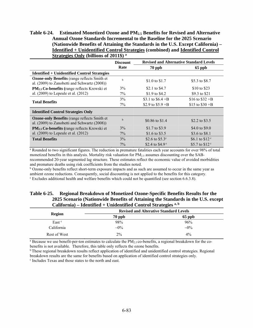
6-83
Table 6-24. Estimated Monetized Ozone and PM2.5 Benefits for Revised and Alternative Annual Ozone Standards Incremental to the Baseline for the 2025 Scenario (Nationwide Benefits of Attaining the Standards in the U.S. Except California) –Identified + Unidentified Control Strategies (combined) and Identified Control Strategies Only (billions of 2011$) a
Discount
Rate Revised and Alternative Standard Levels
70 ppb 65 ppb Identified + Unidentified Control Strategies Ozone-only Benefits (range reflects Smith et al. (2009) to Zanobetti and Schwartz (2008))
b $1.0 to $1.7 $5.3 to $8.7
PM2.5 Co-benefits (range reflects Krewski et al. (2009) to Lepeule et al. (2012)
3% $2.1 to $4.7 $10 to $23 7% $1.9 to $4.2 $9.3 to $21
Total Benefits 3% $3.1 to $6.4 +B $16 to $32 +B 7% $2.9 to $5.9 +B $15 to $30 +B
Identified Control Strategies Only
Ozone-only Benefits (range reflects Smith et al. (2009) to Zanobetti and Schwartz (2008))
b $0.86 to $1.4 $2.2 to $3.5
PM2.5 Co-benefits (range reflects Krewski et al. (2009) to Lepeule et al. (2012)
3% $1.7 to $3.9 $4.0 to $9.0 7% $1.6 to $3.5 $3.6 to $8.1
Total Benefits 3% $2.6 to $5.3c $6.1 to $12 c 7% $2.4 to $4.9 c $5.7 to $12 c
a Rounded to two significant figures. The reduction in premature fatalities each year accounts for over 98% of total monetized benefits in this analysis. Mortality risk valuation for PM2.5 assumes discounting over the SAB-recommended 20-year segmented lag structure. These estimates reflect the economic value of avoided morbidities and premature deaths using risk coefficients from the studies noted. b Ozone-only benefits reflect short-term exposure impacts and as such are assumed to occur in the same year as ambient ozone reductions. Consequently, social discounting is not applied to the benefits for this category. c Excludes additional health and welfare benefits which could not be quantified (see section 6.6.3.8). Table 6-25. Regional Breakdown of Monetized Ozone-Specific Benefits Results for the
2025 Scenario (Nationwide Benefits of Attaining the Standards in the U.S. except California) – Identified + Unidentified Control Strategies a, b
Region Revised and Alterative Standard Levels
70 ppb 65 ppb East c 98% 96%
California ~0% ~0%
Rest of West 2% 4% a Because we use benefit-per-ton estimates to calculate the PM2.5 co-benefits, a regional breakdown for the co-benefits is not available. Therefore, this table only reflects the ozone benefits. b These regional breakdown results reflect application of identified and unidentified control strategies. Regional breakdown results are the same for benefits based on application of identified control strategies only. c Includes Texas and those states to the north and east.
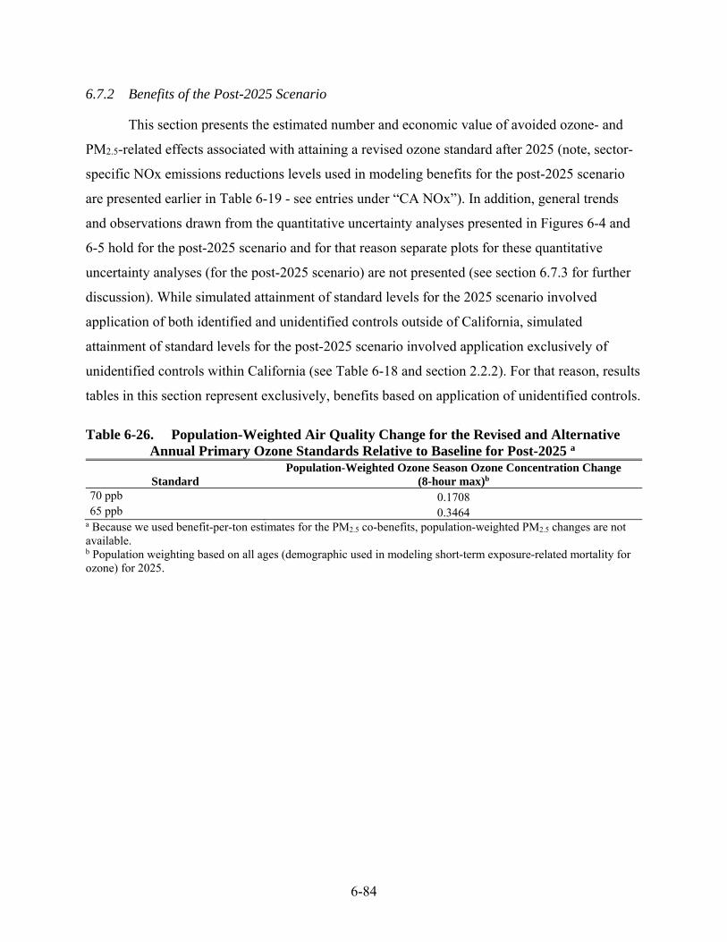
6-84
6.7.2 Benefits of the Post-2025 Scenario
This section presents the estimated number and economic value of avoided ozone- and
PM2.5-related effects associated with attaining a revised ozone standard after 2025 (note, sector-
specific NOx emissions reductions levels used in modeling benefits for the post-2025 scenario
are presented earlier in Table 6-19 - see entries under “CA NOx”). In addition, general trends
and observations drawn from the quantitative uncertainty analyses presented in Figures 6-4 and
6-5 hold for the post-2025 scenario and for that reason separate plots for these quantitative
uncertainty analyses (for the post-2025 scenario) are not presented (see section 6.7.3 for further
discussion). While simulated attainment of standard levels for the 2025 scenario involved
application of both identified and unidentified controls outside of California, simulated
attainment of standard levels for the post-2025 scenario involved application exclusively of
unidentified controls within California (see Table 6-18 and section 2.2.2). For that reason, results
tables in this section represent exclusively, benefits based on application of unidentified controls.
Table 6-26. Population-Weighted Air Quality Change for the Revised and Alternative Annual Primary Ozone Standards Relative to Baseline for Post-2025 a
Standard Population-Weighted Ozone Season Ozone Concentration Change
(8-hour max)b 70 ppb 0.1708 65 ppb 0.3464
a Because we used benefit-per-ton estimates for the PM2.5 co-benefits, population-weighted PM2.5 changes are not available. b Population weighting based on all ages (demographic used in modeling short-term exposure-related mortality for ozone) for 2025.

6-85
Table 6-27. Estimated Number of Avoided Ozone-Related Health Impacts for the Revised and Alternative Annual Ozone Standards (Incremental to the Baseline) for the Post-2025 Scenario (Nationwide Benefits of Attaining the Standards just in California) a, b
a All incidence estimates are rounded to whole numbers with a maximum of two significant digits. b All incidence estimates are based on ozone-only models unless otherwise noted. d The negative estimates at the 5th percentile confidence estimates for these morbidity endpoints reflect the statistical power of the studies used to calculate these health impacts. These results do not suggest that reducing air pollution results in additional health impacts.
70 ppb 65 ppb
Avoided Short-Term Mortality72 150
(35 to 110) (71 to 220)120 240
(64 to 180) (130 to 350)Avoided Long-term Respiratory Mortality
290 590(98 to 480) (200 to 970)
Avoided Morbidity140 270
(-32 to 300) (-65 to 610)
360 720(33 to 1,100) (67 to 2,200)
160,000 330,000(-49,000 to 320,000) (-100,000 to 650,000)
320,000 660,000(130,000 to 510,000) (270,000 to 1,000,000)
120,000 240,000(42,000 to 260,000) (85,000 to 530,000)
Asthma exacerbation (age 6-18)d
Minor restricted-activity days (age 18-65)
School Loss Days (age 5-17)
Hospital admissions - respiratory
(age 65+)d
Emergency department visits for asthma (all ages)
multi-city study
Health Effectb
Revised and Alterative Standard Levels(95th percentile confidence intervals)
multi-city studiesSmith et al. (2009) (all ages)
Zanobetti and Schwartz (2008) (all ages)
Jerrett et al. (2009) (30-99yrs)
copollutants model (PM2.5)

6-86
Table 6-28. Total Monetized Ozone-Only Benefits for the Revised and Alternative Annual Ozone Standards (Incremental to the Baseline) for the Post-2025 Scenario (Nationwide Benefits of Attaining the Standards just in California) (millions of 2011$) a
a All benefits estimates are rounded to whole numbers with a maximum of two significant digits. The monetized value of the ozone-related morbidity benefits are included in the estimates shown in this table for each mortality study
70 ppb 65 ppbAvoided Short-Term Mortality - Core Analysis
$790 $1,600($74 to $2,200) ($150 to $4,500)
1,300 2,600($120 to $3,600) ($240 to $7,200)
multi-city studies
Smith et al. (2009) (all ages)
Zanobetti and Schwartz (2008) (all ages)
Health Effectb
(95th percentile confidence intervals)Revised and Alterative Standard Levels
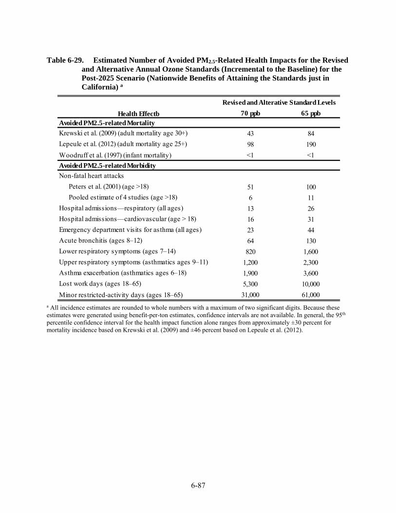
6-87
Table 6-29. Estimated Number of Avoided PM2.5-Related Health Impacts for the Revised
and Alternative Annual Ozone Standards (Incremental to the Baseline) for the Post-2025 Scenario (Nationwide Benefits of Attaining the Standards just in California) a
a All incidence estimates are rounded to whole numbers with a maximum of two significant digits. Because these estimates were generated using benefit-per-ton estimates, confidence intervals are not available. In general, the 95th percentile confidence interval for the health impact function alone ranges from approximately ±30 percent for mortality incidence based on Krewski et al. (2009) and ±46 percent based on Lepeule et al. (2012).
70 ppb 65 ppb
Avoided PM2.5-related Mortality
Krewski et al. (2009) (adult mortality age 30+) 43 84
Lepeule et al. (2012) (adult mortality age 25+) 98 190
Woodruff et al. (1997) (infant mortality) <1 <1
Avoided PM2.5-related Morbidity
Non-fatal heart attacks
Peters et al. (2001) (age >18) 51 100
Pooled estimate of 4 studies (age >18) 6 11
Hospital admissions—respiratory (all ages) 13 26
Hospital admissions—cardiovascular (age > 18) 16 31
Emergency department visits for asthma (all ages) 23 44
Acute bronchitis (ages 8–12) 64 130
Lower respiratory symptoms (ages 7–14) 820 1,600
Upper respiratory symptoms (asthmatics ages 9–11) 1,200 2,300
Asthma exacerbation (asthmatics ages 6–18) 1,900 3,600
Lost work days (ages 18–65) 5,300 10,000
Minor restricted-activity days (ages 18–65) 31,000 61,000
Revised and Alterative Standard Levels
Health Effectb
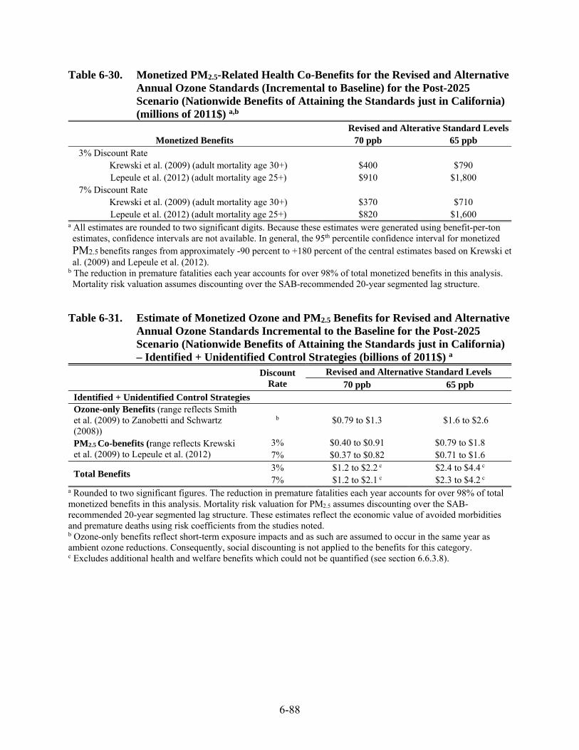
6-88
Table 6-30. Monetized PM2.5-Related Health Co-Benefits for the Revised and Alternative Annual Ozone Standards (Incremental to Baseline) for the Post-2025 Scenario (Nationwide Benefits of Attaining the Standards just in California) (millions of 2011$) a,b Revised and Alterative Standard Levels
Monetized Benefits 70 ppb 65 ppb
3% Discount Rate Krewski et al. (2009) (adult mortality age 30+) $400 $790 Lepeule et al. (2012) (adult mortality age 25+) $910 $1,800
7% Discount Rate Krewski et al. (2009) (adult mortality age 30+) $370 $710 Lepeule et al. (2012) (adult mortality age 25+) $820 $1,600
a All estimates are rounded to two significant digits. Because these estimates were generated using benefit-per-ton estimates, confidence intervals are not available. In general, the 95th percentile confidence interval for monetized PM2.5 benefits ranges from approximately -90 percent to +180 percent of the central estimates based on Krewski et al. (2009) and Lepeule et al. (2012).
b The reduction in premature fatalities each year accounts for over 98% of total monetized benefits in this analysis. Mortality risk valuation assumes discounting over the SAB-recommended 20-year segmented lag structure.
Table 6-31. Estimate of Monetized Ozone and PM2.5 Benefits for Revised and Alternative
Annual Ozone Standards Incremental to the Baseline for the Post-2025 Scenario (Nationwide Benefits of Attaining the Standards just in California) – Identified + Unidentified Control Strategies (billions of 2011$) a
Discount
Rate Revised and Alternative Standard Levels
70 ppb 65 ppb Identified + Unidentified Control Strategies Ozone-only Benefits (range reflects Smith et al. (2009) to Zanobetti and Schwartz (2008))
b $0.79 to $1.3 $1.6 to $2.6
PM2.5 Co-benefits (range reflects Krewski et al. (2009) to Lepeule et al. (2012)
3% $0.40 to $0.91 $0.79 to $1.8 7% $0.37 to $0.82 $0.71 to $1.6
Total Benefits 3% $1.2 to $2.2 c $2.4 to $4.4 c 7% $1.2 to $2.1 c $2.3 to $4.2 c
a Rounded to two significant figures. The reduction in premature fatalities each year accounts for over 98% of total monetized benefits in this analysis. Mortality risk valuation for PM2.5 assumes discounting over the SAB-recommended 20-year segmented lag structure. These estimates reflect the economic value of avoided morbidities and premature deaths using risk coefficients from the studies noted. b Ozone-only benefits reflect short-term exposure impacts and as such are assumed to occur in the same year as ambient ozone reductions. Consequently, social discounting is not applied to the benefits for this category. c Excludes additional health and welfare benefits which could not be quantified (see section 6.6.3.8).
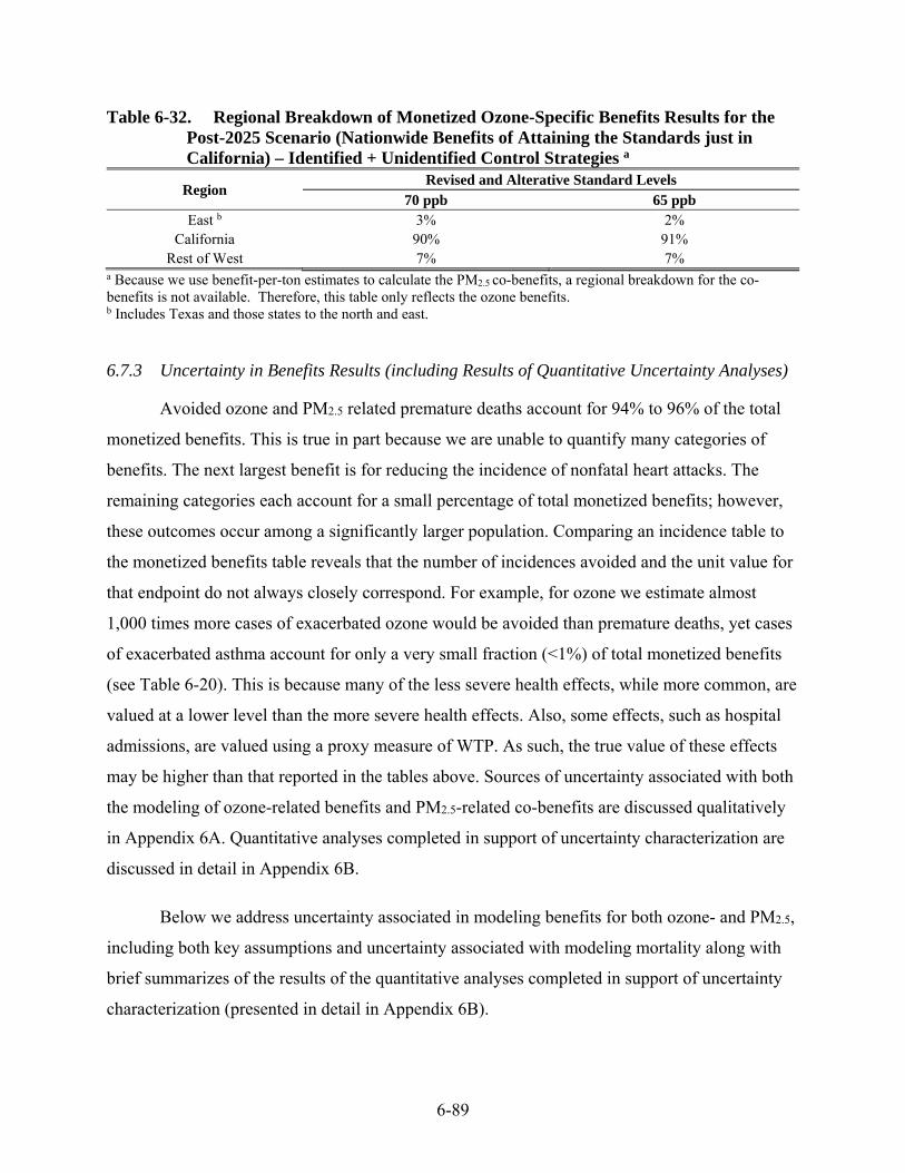
6-89
Table 6-32. Regional Breakdown of Monetized Ozone-Specific Benefits Results for the Post-2025 Scenario (Nationwide Benefits of Attaining the Standards just in California) – Identified + Unidentified Control Strategies a
Region Revised and Alterative Standard Levels
70 ppb 65 ppb East b 3% 2%
California 90% 91% Rest of West 7% 7%
a Because we use benefit-per-ton estimates to calculate the PM2.5 co-benefits, a regional breakdown for the co-benefits is not available. Therefore, this table only reflects the ozone benefits. b Includes Texas and those states to the north and east. 6.7.3 Uncertainty in Benefits Results (including Results of Quantitative Uncertainty Analyses)
Avoided ozone and PM2.5 related premature deaths account for 94% to 96% of the total
monetized benefits. This is true in part because we are unable to quantify many categories of
benefits. The next largest benefit is for reducing the incidence of nonfatal heart attacks. The
remaining categories each account for a small percentage of total monetized benefits; however,
these outcomes occur among a significantly larger population. Comparing an incidence table to
the monetized benefits table reveals that the number of incidences avoided and the unit value for
that endpoint do not always closely correspond. For example, for ozone we estimate almost
1,000 times more cases of exacerbated ozone would be avoided than premature deaths, yet cases
of exacerbated asthma account for only a very small fraction (<1%) of total monetized benefits
(see Table 6-20). This is because many of the less severe health effects, while more common, are
valued at a lower level than the more severe health effects. Also, some effects, such as hospital
admissions, are valued using a proxy measure of WTP. As such, the true value of these effects
may be higher than that reported in the tables above. Sources of uncertainty associated with both
the modeling of ozone-related benefits and PM2.5-related co-benefits are discussed qualitatively
in Appendix 6A. Quantitative analyses completed in support of uncertainty characterization are
discussed in detail in Appendix 6B.
Below we address uncertainty associated in modeling benefits for both ozone- and PM2.5,
including both key assumptions and uncertainty associated with modeling mortality along with
brief summarizes of the results of the quantitative analyses completed in support of uncertainty
characterization (presented in detail in Appendix 6B).
6-90
Ozone-Related Benefits
Key assumption and uncertainties related to modeling of ozone-related premature mortality: Ozone-related short-term mortality represents a substantial proportion of total monetized benefits (over 94% of the ozone-related-benefits), and these estimates have the following key assumptions and uncertainties. We utilize a log-linear impact function without a threshold in modeling short-term ozone-related mortality. However, we acknowledge reduced confidence in specifying the nature of the C-R function in the range of ≤20ppb and below (ozone ISA, section 2.5.4.4). Thus, the estimates include health benefits from reducing ozone in areas with varied concentrations of ozone, including both areas that do not meet the ozone standard and those areas that are in attainment, down to the lowest modeled concentrations.
Avoided premature mortality according to baseline pollutant concentrations: We recognize that, in estimating short-term ozone-related mortality, we are less confident in specifying the shape of the C-R function at lower ambient ozone concentrations (at and below 20 ppb, ozone ISA, section 2.5.4.4). As discussed in section 6.7.3.2 and (in greater detail) in Appendix 6B, section 6B.7, quantitative uncertainty analyses completed for this RIA found that the vast majority (~84%) of the reductions estimated premature mortality for simulated attainment of the revised and alternative standards (70 ppb and 65 ppb) were associated with grid cells having mean 8-hour max values between 35 and 55 ppb. Furthermore, ~100% of mortality reductions occurred above 20 ppb, where we are more confident in specifying the nature of the ozone-mortality effect (ozone ISA, section 2.5.4.4). owever, as discussed in section 6B.7, care must be taken in interpreting these results since the ambient air metric used in modeling this endpoint is the mean 8-hour max value in each grid cell (and not the full distribution of 8-hour daily max values). Had the latter been used, then the distribution would have likely been wider. The use of the mean 8-hour max metric in the RIA also means that the graphical distributions referenced here and presented in Appendix 6B.7 cannot be readily contrasted with specific ozone standard levels (since those are based on 8-hour max daily metrics and not on a seasonal-mean of those metrics).
Short-term ozone-exposure related premature mortality (alternative epidemiological studies and C-R functions): We estimated the number of premature deaths using seven additional effect estimates including four multi-city studies and three meta-analysis studies. This quantitative uncertainty analysis showed that the two core incidence and benefits estimates fall within (and towards the lower end of) the broader range resulting from application of the seven alternative effect estimates (see Figure 6-4).
Economic value of avoided premature mortality from long-term exposure to ozone: We estimated the economic value of long-term ozone mortality using two cessation lag structures: 20-year segment lag (as used for PM2.5) and a zero lag. The quantitative uncertainty analysis suggests that if included in the core benefit estimate, long-term ozone exposure-related mortality could add substantially to the overall benefits. Additionally, use of a 20-year segment lag can reduce benefits by 10-20% (relative to a zero lag) depending on the discount rate applied.

6-91
Long-term ozone-exposure related premature respiratory mortality and potential thresholds: We evaluated the impact of several assumed thresholds ranging from 40-60 ppb. This quantitative uncertainty analysis suggested that a threshold of 50 ppb or greater could have a substantial impact on estimated benefits, while thresholds below this range have a relatively minor impact.
Income elasticity for premature mortality and certain morbidity endpoints: We examined the impact of alternative assumptions regarding income elasticity (i.e., the degree to which WTP changes as income changes) and the degree of impact on WTP functions used for mortality and for morbidity endpoints. That quantitative uncertainty analysis suggests that alternative assumptions regarding income elasticity could result in a moderate impact on mortality benefits (values ranging from ~90% to ~130% of the core estimate depending on the assumption regarding elasticity). Income elasticity was found to have a far more modest impact on morbidity endpoints modeled using WTP functions.
Value of increased productivity among outdoor agricultural workers due to reduced exposure to ozone: Using information from the Graff Zivin and Neidell (2012) study, we estimate the economic value of improved productivity among outdoor non-livestock workers for the ozone standards in 2025 in our uncertainty analysis. We estimate the monetized worker productivity benefits of attaining a 70 ppb standard would be about $1.7 million and a 65 ppb standard would yield monetized benefits of about $8.9 million.165
PM2.5-Related Benefits
Key assumption and uncertainties related to modeling of PM2.5-related premature mortality PM2.5 mortality co-benefits represent a substantial proportion of total monetized benefits (over 98% of the co-benefits), and these estimates have the following key assumptions and uncertainties. We assume that all fine particles, regardless of their chemical composition, are equally potent in causing premature mortality. This is an important assumption, because PM2.5 produced varies considerably in composition across sources, but the scientific evidence is not yet sufficient to allow differential effects estimates by particle type. The PM ISA, which was twice reviewed by SAB-CASAC, concluded that “many constituents of PM2.5 can be linked with multiple health effects, and the evidence is not yet sufficient to allow differentiation of those constituents or sources that are more closely related to specific outcomes” (U.S. EPA, 2009b). We assume further that the health impact function for fine particles is log-linear without a threshold in this analysis. Thus, the estimates include health benefits from reducing fine particles in areas with varied concentrations of PM2.5, including both areas that do not meet the fine particle standard and those areas that are in attainment, down to the lowest modeled concentrations. In addition, we assume that there is a “cessation” lag between
165 We recognize that there is significant uncertainty in the generalizability of this study and the need for additional research and peer review in guiding the monetization of agriculatural productivity impacts.
6-92
the change in PM exposures and the total realization of changes in mortality effects. Specifically, we assume that some of the incidences of premature mortality related to PM2.5 exposures occur in a distributed fashion over the 20 years following exposure based on the advice of the SAB-HES (U.S. EPA-SAB, 2004c), which affects the valuation of mortality benefits at different discount rates. And finally, we recognize uncertainty associated with application of the benefit-per-ton approach used in modeling PM2.5 co-benefits. The benefit-per-ton estimates used here reflect specific geographic patterns of emissions reductions and specific air quality and benefits modeling assumptions associated with the derivation of those estimates (see the TSD describing the calculation of the national benefit-per-ton estimates (U.S. EPA, 2013b) and Fann et al. (2012b). Consequently, these estimates may not reflect local variability in population density, meteorology, exposure, baseline health incidence rates, or other local factors associated with the current ozone NAAQS review. Therefore, use of these benefit-per-ton values to estimate co-benefits may lead to higher or lower benefit estimates than if co-benefits were calculated based on direct air quality modeling.
Avoided premature mortality according to baseline pollutant concentrations: We recognize that, in modeling long-term PM2.5-related mortality, we are less confident in specifying the shape of the C-R function at levels below the lowest measured level (LML) reported in the epidemiology study(s) providing the effect estimates used in modeling the mortality endpoint. As discussed in section 6.7.3.2 and (in greater detail) in Appendix 6B, section 6B.7, quantitative analyses completed in support of uncertainty characterization completed for this RIA found that, depending on the mortality study, between 67% and 93% of the long-term PM2.5- related mortality estimate is based on modeling involving baseline PM2.5 levels above the LML. This increases our overall confidence in the mortality estimates underlying the benefit-per-ton values used in the RIA.
Long-term PM2.5 exposure-related premature mortality and alternative C-R functions (based on the Expert Elicitation): We applied the set of expert elicitation-based functions to generate an alternative set of PM2.5 benefit estimates (see Figure 6-5). The estimates based on Krewski et al. (2009) and Lepeule et al. (2012) fall within the range of estimates based on the functions from the 2006 expert elicitation.
6.8 Discussion
This analysis demonstrates the potential for significant health benefits of the illustrative
emissions controls applied to simulate attainment with the revised and alternative primary ozone
standard levels. We estimate that by 2025, the emissions reductions to reach the revised and
alternative standard levels everywhere except California, would have reduced the number of
ozone- and PM2.5-related premature mortalities and produce substantial non-mortality benefits.
Furthermore, emissions reductions required to meet alternative standards in California post-2025
are also likely to produce substantial reductions in these same endpoints. This rule would also

6-93
yield significant welfare impacts as well (see Chapter 7). Even considering the quantified and
unquantified uncertainties identified in this chapter, we believe that the revised and alternative
standards would have substantial public health benefits that are likely to outweigh the costs of
the control strategies for the revised and alternative standard levels analyzed (see Chapter 4).
Inherent in any complex RIA such as this one are multiple sources of uncertainty. Some
of these we characterized through our quantification of statistical error in the C-R relationships
and our use of alternate mortality functions. Others, including the projection of atmospheric
conditions and source-level emissions, the projection of baseline morbidity rates, incomes and
technological development are unquantified. When evaluated within the context of these
uncertainties, the health impact and monetized benefits estimates in this RIA can provide useful
information regarding the public health benefits associated with the revised and alternative
standard levels.
As discussed in Chapter 1, there are important differences worth noting in the design and
analytical objectives of NAAQS RIAs compared to RIAs for implementation rules, such as the
Tier 3 (U.S. EPA, 2014a). Setting a NAAQS does not directly result in costs or benefits. The
NAAQS RIAs illustrate the potential costs and benefits of the revised and alternative air quality
standards nationwide based on an array of emissions reduction strategies for different sources,
incremental to implementation of existing regulations and controls needed to attain the current
standards. In short, NAAQS RIAs hypothesize, but do not predict, the emissions reduction
strategies that States may choose to enact when implementing a revised NAAQS, and as such, by
contrast, the emissions reductions from implementation rules are generally for specific, well-
characterized sources, such as the recent MATS rule (U.S. EPA, 2011c). In general, the EPA is
more confident in the magnitude and location of the emissions reductions for implementation
rules. As such, emissions reductions achieved under promulgated implementation rules, such as
MATS, have been reflected in the baseline of this NAAQS analysis.166 For this reason, the
benefits estimated provided in this RIA and all other NAAQS RIAs should not be added to the
166 The full set of rules reflected in the baseline are presented in Chapter 2, Section 2.1.3.

6-94
benefits estimated for implementation rules. Subsequent implementation rules will be reflected
in the baseline for the next ozone NAAQS review.
In setting the NAAQS, the EPA considers that ozone concentrations vary over space and
time. While the standard is designed to limit concentrations at the highest monitor in an area, it is
understood that emissions controls put in place to reduce concentrations at the highest monitor
will simultaneously result in lower ozone concentrations throughout the entire area. In fact, the
ozone HREA (U.S. EPA, 2014b) shows how different standard levels would affect the entire
distribution of ozone concentrations, and thus people’s exposures and risk, across a selected set
of urban areas. For this reason, it is inappropriate to use the NAAQS level as a bright line for
health effects.
The NAAQS are not set at levels that eliminate the risk of air pollution completely.
Instead, the Administrator sets the NAAQS at a level requisite to protect public health with an
adequate margin of safety, taking into consideration effects on susceptible populations based on
the scientific literature. The risk analysis prepared in support of this ozone NAAQS reported
risks below these levels, while acknowledging that the confidence in those effect estimates is
higher at levels closer to the standard (U.S. EPA, 2014b). While benefits occurring below the
standard may be somewhat more uncertain than those occurring above the standard, the EPA
considers these to be legitimate components of the total benefits estimate. Though there are
greater uncertainties at lower ozone and PM2.5 concentrations, there is no evidence of a threshold
in short-term ozone or PM2.5-related health effects in the epidemiology literature. Given that the
epidemiological literature in most cases has not provided estimates based on threshold models,
there would be additional uncertainties imposed by assuming thresholds or other non-linear C-R
functions for the purposes of benefits analysis.
The estimated benefits shown here are in addition to the substantial benefits estimated for
several recent air quality rules (U.S. EPA, 2009a, 2011c, 2014a). Emissions reductions from
rules such as Tier 3 will have substantially reduced ambient ozone concentrations by 2025 in the
East, such that few additional controls would be needed to reach 70 ppb. These rules that have
already been promulgated have tremendous combined benefits that explain why the number of
avoided premature mortality associated with this NAAQS revision are smaller than were

6-95
estimated in the previous ozone NAAQS RIA (U.S. EPA, 2006) for the year 2020 and even
smaller than the mortality risks estimated for the current year in the ozone HREA (U.S. EPA,
2014b).
6.9 References
Adams PF, Hendershot GE, Marano MA. 1999. “Current Estimates from the National Health Interview Survey, 1996.” Vital and Health Statistics 10(200):1-212.
Agency for Healthcare Research and Quality (AHRQ). 2000. HCUPnet, Healthcare Cost and Utilization Project. Rockville, MD. Available at <http://hcupnet.ahrq.gov>.
Agency for Healthcare Research and Quality (AHRQ). 2007. HCUPnet, Healthcare Cost and Utilization Project. Rockville, MD. Available at <http://hcupnet.ahrq.gov>.
Agency for Healthcare Research and Quality (AHRQ). 2009. HCUPnet, Healthcare Cost and Utilization Project. Rockville, MD. Available at <http://hcupnet.ahrq.gov>.
Alberini A, Cropper M, Krupnick A, Simon NB. 2004. “Does the value of a statistical life vary with age and health status? Evidence from the US and Canada.” Journal of Environmental Economics and Management 48(1): 769-792.
Alberini, Anna & Milan Ščasný. 2011. "Context and the VSL: Evidence from a Stated Preference Study in Italy and the Czech Republic." Environmental & Resource Economics 49(4), pages 511-538.
Aldy JE, Viscusi WK. 2008. “Adjusting the value of a statistical life for age and cohort effects.” The Review of Economics and Statistics 90(3):573-581.
American Lung Association (ALA). 2002. Trends in Asthma Morbidity and Mortality. American Lung Association, Best Practices and Program Services, Epidemiology and Statistics Unit. Available at <http://www.lungusa.org/data/asthma/ASTHMAdt.pdf>.
American Lung Association (ALA). 2010. Trends in Asthma Morbidity and Mortality. American Lung Association Epidemiology and Statistics Unit Research and Program Services Division. February. Table 7. Based on NHIS data (CDC, 2008). Available at http://www.lungusa.org/finding-cures/our-research/trend-reports/asthma-trend-report.pdf.
Ayyub, B.M. 2002. Elicitation of Expert Opinions for Uncertainty and Risk. CRC Press, Florida.
Babin, S. M., H. S. Burkom, et al. 2007. “Pediatric Patient Asthma-related Emergency Department Visits and Admissions in Washington, DC, from 2001–2004, and Associations with Air Quality, Socio-economic Status and Age Group.” Environmental Health 6: 9.
Barnett AG; Williams GM; Schwartz J; Best TL; Neller AH; Petroeschevsky AL; Simpson RW. 2006. The effects of air pollution on hospitalizations for cardiovascular disease in elderly people in Australian and New Zealand cities. Environ Health Perspect, 114: 1018-1023.
Bell ML; Ebisu K; Peng RD; Walker J; Samet JM; Zeger SL; Dominic F. 2008. Seasonal and regional short-term effects of fine particles on hospital admissions in 202 U.S. counties, 1999-2005. Am J Epidemiol, 168: 1301-1310.

6-96
Bell, M.L.; A. McDermott; S.L. Zeger; J.M. Samet; F. Dominici. 2004. Ozone and short-term mortality in 95 U.S. urban communities, 1987-2000. JAMA. 292:2372-2378.
Bell, ML; Dominici, F; Samet, JM. 2005. Ameta-analysis of time-series studies of ozone and mortality with comparison to the national morbidity, mortality, and air pollution study. Epidemiology 16: 436-445. http://dx.doi.org/10.1097/01.ede.0000165817.40152.85
Bell, ML; McDermott, A; Zeger, SL; Samet, JM; Dominici, F. 2004. Ozone and short-term mortality in 95 US urban communities, 1987-2000. JAMA 292: 2372-2378. http://dx.doi.org/10.1001/jama.292.19.2372
Berger, M.C., G.C. Blomquist, D. Kenkel, and G.S. Tolley. 1987. “Valuing Changes in Health Risks: A Comparison of Alternative Measures.” The Southern Economic Journal 53:977-984.
Centers for Disease Control and Prevention (CDC). 2008. National Center for Health Statistics. National Health Interview Survey, 1999-2008.
Chen L, Jennison BL, Yang W, and Omaye ST. 2000. “Elementary school absenteeism and air pollution.” Inhalation Toxicolology 12(11):997-1016.
Crocker, T. D., & Horst, R. L. 1981. Hours of work, labor productivity, and environmental conditions: A case study. The Review of Economics and Statistics, 63(3), 361-368.
Cropper, M. L. and A. J. Krupnick. 1990. The Social Costs of Chronic Heart and Lung Disease. Resources for the Future. Washington, DC. Discussion Paper QE 89-16-REV.
Dockery DW; Pope CA III; Xu X; Spengler JD; Ware JH; Fay ME; Ferris BG Jr; Speizer FE. 1993. An association between air pollution and mortality in six US cities. N Engl J Med, 329: 1753-1759.
Dockery, D.W., J. Cunningham, A.I. Damokosh, L.M. Neas, J.D. Spengler, P. Koutrakis, J.H. Ware, M. Raizenne, and F.E. Speizer. 1996. “Health Effects of Acid Aerosols On North American Children-Respiratory Symptoms.” Environmental Health Perspectives 104(5):500-505.
Eisenstein, E.L., L.K. Shaw, K.J. Anstrom, C.L. Nelson, Z. Hakim, V. Hasselblad and D.B. Mark. 2001. “Assessing the Clinical and Economic Burden of Coronary Artery Disease: 1986-1998.” Medical Care 39(8):824-35.
Fann N, Fulcher C.M., Hubbell B.J. 2009. The influence of location, source, and emission type in estimates of the human health benefits of reducing a ton of air pollution. Air Qual Atmos Health (2009) 2:169–176
Fann N, Lamson A, Wesson K, Risley D, Anenberg SC, Hubbell BJ. 2012a. “Estimating the National Public Health Burden Associated with Exposure to Ambient PM2.5 and ozone. Risk Analysis,” Risk Analysis 32(1): 81-95.
Fann N, Baker K R, Fulcher, C M. 2012b. Characterizing the PM2.5-related health benefits of emission reductions for 17 industrial, area and mobile emission sectors across the U.S. Environment International 49 (2012) 141–151.
Freeman (III), AM. 1993. The Measurement of Environmental and Resource Values: Theory and Methods. Washington, DC: Resources for the Future.
Gent, J.F.; E.W. Triche; T.R. Holford; K. Belanger; M.B. Bracken; W.S. Beckett, et al. 2003. Association of low-level ozone and fine particles with respiratory symptoms in children with asthma. Journal of the American Medical Association. 290(14):1859-1867.
GeoLytics Inc. 2002. GeoLytics CensusCD® 2000 Short Form Blocks. CD-ROM Release 1.0. GeoLytics, Inc. East Brunswick, NJ. Available: http://www.geolytics.com/ [accessed 29 September 2004].

6-97
Gilliland FD, Berhane K, Rappaport EB, Thomas DC, Avol E, Gauderman WJ, et al. 2001. “The effects of ambient air pollution on school absenteeism due to respiratory illnesses.” Epidemiology 12(1):43-54.
Glad, J.A., L.L. Brink, E.O. Talbott, P.C. Lee, X. Xu, M. Saul, and J. Rager. 2012. “The Relationship of Ambient ozone and PM2.5 Levels and Asthma Emergency Department Visits: Possible Influence of Gender and Ethnicity.” Archives of Environmental & Occupational Health 62 (2): 103-108.
Graff Zivin, J., Neidell, M. 2012. “The impact of pollution on worker productivity.” American Economic Review, 102, 3652-3673.
Hall JV, Brajer V, Lurmann FW. 2003. “Economic Valuation of ozone-related School Absences in the South Coast Air Basin of California.” Contemporary Economic Policy 21(4):407-417.
Harrington, W., and P.R. Portney. 1987. “Valuing the Benefits of Health and Safety Regulation.” Journal of Urban Economics 22:101-112.
Hollman, F.W., T.J. Mulder, and J.E. Kallan. 2000. Methodology and Assumptions for the Population Projections of the United States: 1999 to 2100. Population Division Working Paper No. 38, Population Projections Branch, Population Division, U.S. Census Bureau, Department of Commerce. January. Available at <http://www.census.gov/population/www/documentation/twps0038/twps0038.html>.
Huang, Y., Dominici, F., & Bell, M. L. 2005. Bayesian Hierarchical Distributed Lag Models for Summer Ozone Exposure and Cardio-Respiratory Mortality. Environmetrics, 16, 547-562.
Hubbell B, Fann N, Levy J. 2009. Methodological considerations in developing local-scale health impact assessments: balancing national, regional, and local data. Air Qual. Atmos. Heal. 2:99–110; doi:10.1007/s11869-009-0037-z.
Hubbell, B., A. Hallberg, D.R. McCubbin, and E. Post. 2005. “Health-Related Benefits of Attaining the 8-Hr Ozone Standard.” Environmental Health Perspectives 113:73–82. ICD, 1979
Industrial Economics, Incorporated (IEc). 2006. Expanded Expert Judgment Assessment of the Concentration-Response Relationship Between PM2.5 Exposure and Mortality. Prepared for: Office of Air Quality Planning and Standards, U.S. Environmental Protection Agency, Research Triangle Park, NC. September. Available on the Internet at <http://www.epa.gov/ttn/ecas/regdata/Uncertainty/pm_ee_tsd_expert_interview_summaries.pdf>.
Industrial Economics, Incorporated (IEc). 2012. Updating BenMAP Income Elasticity Estimates—Literature Review. Prepared for: Office of Air Quality Planning and Standards, U.S. Environmental Protection Agency, Research Triangle Park, NC. September. Available at <http://www.epa.gov/ttn/ecas/regdata/Benefits/IncomeElasticityUpdate_Recommendationswithappendices.pdf>
Ito, K.; G.D. Thurston and R.A. Silverman. 2007. Characterization of PM2.5, gaseous pollutants, and meteorological interactions in the context of time-series health effects models. Journal of Exposure Science and Environmental Epidemiology. 17(S2):S45-60.
Ito, K; De Leon, SF; Lippmann, M. 2005. Associations between ozone and daily mortality, analysis and meta-analysis. Epidemiology 16: 446-457.
Jerrett M, Burnett RT, Pope CA, III, et al. 2009. “Long-Term Ozone Exposure and Mortality.” New England Journal of Medicine 360:1085-95.
Katsouyanni, K.; J.M. Samet; H.R. Anderson; R. Atkinson; A.L. Tertre; S. Medina, et al. 2009. Air Pollution and Health: A European and North American Approach (APHENA). Health Effects Institute.

6-98
Kleckner, N., and J. Neumann. 1999. Recommended Approach to Adjusting WTP Estimates to Reflect Changes in Real Income. Memorandum to Jim DeMocker, U.S. EPA/OPAR. June 3. Available at <http://www.epa.gov/ttn/ecas/regdata/Benefits/background/klecknerandneumann1999.pdf>.
Kloog, I., B.A. Coull, A. Zanobetti, P. Koutrakis, J.D. Schwartz. 2012. “Acute and Chronic Effects of Particles on Hospital Admissions in New England.” PLoS ONE. Vol 7 (4): 1-8.
Kochi, I., B. Hubbell, and R. Kramer. 2006. “An Empirical Bayes Approach to Combining Estimates of the Value of Statistical Life for Environmental Policy Analysis.” Environmental and Resource Economics. 34: 385-406.
Krewski D, Jerrett M, Burnett RT, Ma R, Hughes E, Shi, Y, et al. 2009. Extended follow-up and spatial analysis of the American Cancer Society study linking particulate air pollution and mortality. HEI Research Report, 140, Health Effects Institute, Boston, MA.
Kunzli, N., R. Kaiser, S. Medina, M. Studnicka, O. Chanel, P. Filliger, M. Herry, F. Horak Jr., V. Puybonnieux-Texier, P. Quenel, J. Schneider, R. Seethaler, J-C Vergnaud, and H. Sommer. 2000. “Public-Health Impact of Outdoor and Traffic-Related Air Pollution: A European Assessment.” The Lancet 356:795-801.
Kunzli, N., S. Medina, R. Kaiser, P. Quenel, F. Horak Jr, and M. Studnicka. 2001. “Assessment of Deaths Attributable to Air Pollution: Should We Use Risk Estimates Based on Time Series or on Cohort Studies?” American Journal of Epidemiology 153(11):1050-55.
Laden, F., J. Schwartz, F.E. Speizer, and D.W. Dockery. 2006. “Reduction in Fine Particulate Air Pollution and Mortality.” American Journal of Respiratory and Critical Care Medicine 173:667-672.
Lepeule J, Laden F, Dockery D, Schwartz J. 2012. “Chronic Exposure to Fine Particles and Mortality: An Extended Follow-Up of the Harvard Six Cities Study from 1974 to 2009.” Environmental Health Perspectives 120 (7):965-70.
Levy JI, Baxter LK, Schwartz J. 2009. “Uncertainty and variability in health-related damages from coal-fired power plants in the United States.” Risk Analysis 29(7) 1000-1014.
Levy, JI; Chemerynski, SM; Sarnat, JA. 2005. Ozone exposure and mortality, an empiric Bayes metaregression analysis. Epidemiology 16: 458-468.
Lichtenstein, S. and P. Slovic, eds. 2006. The construction of preference. New York: Cambridge University Press.
Mansfield, Carol; Paramita Sinha; Max Henrion. 2009. Influence Analysis in Support of Characterizing Uncertainty in Human Health Benefits Analysis: Final Report. Prepared for U.S. EPA, Office of Air Quality Planning and Standards. November. Available at <http://www.epa.gov/ttn/ecas/regdata/Benefits/influence_analysis_final_report_psg.pdf>.
Mar, T. F., J. Q. Koenig and J. Primomo. 2010. “Associations between asthma emergency visits and particulate matter sources, including diesel emissions from stationary generators in Tacoma, Washington.” Inhalation Toxicology 22 (6): 445-8.
Mar, T. F., J. Q. Koenig and J. Primomo. 2010. “Associations between asthma emergency visits and particulate matter sources, including diesel emissions from stationary generators in Tacoma, Washington.” Inhal Toxicol. Vol. 22 (6): 445-8.Mar, T. F., T. V. Larson, et al. 2004. “An analysis of the association between respiratory symptoms in subjects with asthma and daily air pollution in Spokane, Washington.” Inhal Toxicol 16(13): 809-15.
Mar, T. F., T. V. Larson, et al. 2004. “An analysis of the association between respiratory symptoms in subjects with asthma and daily air pollution in Spokane, Washington.” Inhalation Toxicology 16(13): 809-15.

6-99
Mar, TF; Koenig, JQ. 2009. Relationship between visits to emergency departments for asthma and ozone exposure in greater Seattle, Washington. Ann Allergy Asthma Immunol 103: 474-479.http://dx.doi.org/10.1016/S1081-1206(10)60263-3
Moolgavkar, S.H. 2000. “Air Pollution and Hospital Admissions for Diseases of the Circulatory System in Three U.S. Metropolitan Areas.” Journal of the Air and Waste Management Association 50:1199-1206.
Mortimer, KM; Neas, LM; Dockery, DW; Redline, S; Tager, IB. 2002. The effect of air pollution on innercity children with asthma. Eur Respir J 19: 699-705.
Mrozek, J.R., and L.O. Taylor. 2002. “What Determines the Value of Life? A Meta-Analysis.” Journal of Policy Analysis and Management 21(2):253-270.
Mustafić H, Jabre P, Caussin C et al. 2012. “Main Air Pollutants and Myocardial Infarction: A Systematic Review and Meta-analysis” JAMA. 2012;307(7):713-721.
National Research Council (NRC). 2002. Estimating the Public Health Benefits of Proposed Air Pollution Regulations. Washington, DC: The National Academies Press. Washington, DC.
National Research Council (NRC). 2008. Estimating Mortality Risk Reduction and Economic Benefits from Controlling Ozone Air Pollution. National Academies Press. Washington, DC.
Neumann, J.E., M.T. Dickie, and R.E. Unsworth. 1994. Linkage between Health Effects Estimation and Morbidity Valuation in the Section 812 Analysis—Draft Valuation Document. Industrial Economics Incorporated (IEc) Memorandum to Jim DeMocker, U.S. Environmental Protection Agency, Office of Air and Radiation, Office of Policy Analysis and Review. March 31. Available at <http://www.epa.gov/ttn/ecas/regdata/Benefits/background/neumannn1994.pdf>.
O'Connor, GT; Neas, L; Vaughn, B; Kattan, M; Mitchell, H; Crain, EF; III, ER; Gruchalla, R; Morgan, W; Stout, J; Adams, GK; Lippmann, M. 2008. Acute respiratory health effects of air pollution on children with asthma in US inner cities. J Allergy Clin Immunol 121: 1133-1139.
Office of Management and Budget (OMB). 2003. Circular A-4: Regulatory Analysis. Washington, DC. Available at <http://www.whitehouse.gov/omb/circulars/a004/a-4.html.>
Ostro, B., M. Lipsett, J. Mann, H. Braxton-Owens, and M. White. 2001. “Air Pollution and Exacerbation of Asthma in African-American Children in Los Angeles.” Epidemiology 12(2):200–208.
Ostro, B.D. 1987. “Air Pollution and Morbidity Revisited: A Specification Test.” Journal of Environmental Economics Management 14:87-98.
Ostro, B.D. and S. Rothschild. 1989. “Air Pollution and Acute Respiratory Morbidity: An Observational Study of Multiple Pollutants.” Environmental Research 50:238-247.
Patel, M. M., S. N. Chillrud, J. C. Correa, Y. Hazi, M. Feinberg, D. Kc, S. Prakash, J. M. Ross, D. Levy and P. L. Kinney. 2010. “Traffic-Related Particulate Matter and Acute Respiratory Symptoms among New York City Area Adolescents.” Environ Health Perspect. Sep;118(9):1338-43.
Peel, J.L., P.E. Tolbert, M. Klein et al. 2005. Ambient air pollution and respiratory emergency department visits. Epidemiology. Vol. 16 (2): 164-74.
Peng, R. D., H. H. Chang, et al. 2008. “Coarse particulate matter air pollution and hospital admissions for cardiovascular and respiratory diseases among Medicare patients.” Journal of the American Medical Association 299(18): 2172-9.
6-100
Peng, R. D., M. L. Bell, et al. 2009. “Emergency admissions for cardiovascular and respiratory diseases and the chemical composition of fine particle air pollution.” Environmental Health Perspectives 117(6): 957-63.
Peters A. 2005. “Particulate matter and heart disease: evidence from epidemiological studies.” Toxicology and Applied Pharmacology Sept 1;207(2 Suppl):477-82.
Peters, A., D. W. Dockery, J. E. Muller and M. A. Mittleman. 2001. “Increased particulate air pollution and the triggering of myocardial infarction.” Circulation 103 (23): 2810-5.
Poloniecki, J.D., R.W. Atkinson., A.P. de Leon., and H.R. Anderson. 1997. “Daily Time Series for Cardiovascular Hospital Admissions and Previous Day’s Air Pollution in London, UK.” Occupational and Environmental Medicine 54(8):535-540
Pope CA III; Thun MJ; Namboodiri MM; Dockery DW; Evans JS; Speizer FE; Heath CW Jr (1995). Particulate air pollution as a predictor of mortality in a prospective study of US adults. Am J Respir Crit Care Med, 151: 669-674.
Pope, C. A., III, J. B. Muhlestein, et al. 2006. “Ischemic heart disease events triggered by short-term exposure to fine particulate air pollution.” Circulation 114(23): 2443-8.
Pope, C.A., III, D.W. Dockery, J.D. Spengler, and M.E. Raizenne. 1991. “Respiratory Health and PM10 Pollution: A Daily Time Series Analysis.” American Review of Respiratory Diseases 144:668-674.
Pope, C.A., III, R.T. Burnett, G.D. Thurston, M.J. Thun, E.E. Calle, D. Krewski, and J.J. Godleski. 2004. “Cardiovascular Mortality and Long-term Exposure to Particulate Air Pollution.” Circulation 109: 71-77.
Pope, C.A., III, R.T. Burnett, M.J. Thun, E.E. Calle, D. Krewski, K. Ito, and G.D. Thurston. 2002. “Lung Cancer, Cardiopulmonary Mortality, and Long-term Exposure to Fine Particulate Air Pollution.” Journal of the American Medical Association 287:1132-1141.
Ransom MR, Pope CA III. 1992. Elementary school absences and PM10 pollution in Utah Valley. Environ Res 58:204–219
Roman, Henry A., Katherine D. Walker, Tyra L. Walsh, Lisa Conner, Harvey M. Richmond, Bryan J. Hubbell, and Patrick L. Kinney. 2008. “Expert Judgment Assessment of the Mortality Impact of Changes in Ambient Fine Particulate Matter in the U.S.” Environmental Science & Technology 42(7):2268-2274.
Rosamond, W., G. Broda, E. Kawalec, S. Rywik, A. Pajak, L. Cooper, and L. Chambless. 1999. “Comparison of Medical Care and Survival of Hospitalized Patients with Acute Myocardial Infarction in Poland and the United States.” American Journal of Cardiology 83:1180-1185
Rowe, R.D., and L.G. Chestnut. 1986. “Oxidants and Asthmatics in Los Angeles: A Benefits Analysis—Executive Summary.” Prepared by Energy and Resource Consultants, Inc. Report to the U.S. Environmental Protection Agency, Office of Policy Analysis. EPA- 230-09-86-018. Washington, DC.
Rowlatt, P., Spackman, M., Jones, S., Jones-Lee, M., Loomes, G. 1998. Valuation of deaths from air pollution. A Report for the Department of Environment, Transport and the Regions and the Department of Trade and Industry. National Economic Research Associates (NERA), London.
Russell, M.W., D.M. Huse, S. Drowns, E.C. Hamel, and S.C. Hartz. 1998. “Direct Medical Costs of Coronary Artery Disease in the United States.” American Journal of Cardiology 81(9):1110-1115.
Sarnat, J. A., Sarnat, S. E., Flanders, W. D., Chang, H. H., Mulholland, J., Baxter, L., Ozkaynak, H. 2013. Spatiotemporally resolved air exchange rate as a modifier of acute air pollution-related morbidity in Atlanta. J Expo Sci Environ Epidemiol. doi: 10.1038/jes.2013.32

6-101
Sasser, E. 2014. Response to Comments Regarding the Potential Use of a Threshold Model in Estimating the Mortality Risks from Long-term Exposure to Ozone in the Health Risk and Exposure Assessment for Ozone, Second External Review Draft. Memorandum to Holly Stallworth, Designated Federal Officer, Clean Air Scientific Advisory Committee from EPA/OAQPS Health and Environmental Impacts Division.
Schildcrout, J. S., Sheppard, L., Lumley, T., Slaughter, J. C., Koenig, J. Q., & Shapiro, G. G. (2006). Ambient air pollution and asthma exacerbations in children: an eight-city analysis. Am J Epidemiol, 164(6), 505-517.
Schwartz J, Dockery DW, Neas LM, Wypij D, Ware JH, Spengler JD, Koutrakis P, Speizer FE, Ferris BG Jr. 1994. “Acute effects of summer air pollution on respiratory symptom reporting in children.” American Journal of Respiratory and Critical Care Medicine 150(5 Pt 1):1234-42.
Schwartz, J. 2005. How sensitive is the association between ozone and daily deaths to control for temperature? Am J Respir Crit Care Med 171: 627-631.
Schwartz, J., and L.M. Neas. 2000. “Fine Particles are More Strongly Associated than Coarse Particles with Acute Respiratory Health Effects in Schoolchildren.” Epidemiology 11:6-10.
Sheppard, L. 2003. “Ambient Air Pollution and Nonelderly Asthma Hospital Admissions in Seattle, Washington, 1987-1994.” In Revised Analyses of Time-Series Studies of Air Pollution and Health. Special Report. Boston, MA: Health Effects Institute.
Shogren, J., and T. Stamland. 2002. “Skill and the Value of Life.” Journal of Political Economy 110:1168-1197.
Silverman, R.A.; and K. Ito. 2010. Age-related association of fine particles and ozone with severe acute asthma in New York City. Journal of Allergy Clinical Immunology. 125(2):367-373.
Slaughter, James C et al. 2005. “Association between particulate matter and emergency room visits, hospital admissions and mortality in Spokane, Washington.” Journal of Exposure Analysis and Environmental Epidemiology 15, 153–159.
Smith et al. 2004. “Do the Near Elderly Value Mortality Risks Differently?” The Review of Economics and Statistics 86(1): 423-429.
Smith, D.H., D.C. Malone, K.A. Lawson, L.J. Okamoto, C. Battista, and W.B. Saunders. 1997. “A National Estimate of the Economic Costs of Asthma.” American Journal of Respiratory and Critical Care Medicine 156(3 Pt 1):787-793.
Smith, K., Pattanayak SK, Van Houtven G. 2006. “Structural benefit transfer: An example using VSL estimates.” Ecological Economics 60: 361-371.
Smith, R.L.; B. Xu and P. Switzer. 2009. Reassessing the relationship between ozone and short- term mortality in U.S. urban communities. Inhalation Toxicology. 21:37-61.
Standard and Poor’s. 2000. “The U.S. Economy: The 25 Year Focus.” Winter. Available at <http://:www.standardandpoors.com>.
Stanford, R., T. McLaughlin and L. J. Okamoto. 1999. “The cost of asthma in the emergency department and hospital.” American Journal of Respiratory and Critical Care Medicine 160 (1): 211-5.
Sullivan, J., L. Sheppard, et al. 2005. “Relation between short-term fine-particulate matter exposure and onset of myocardial infarction.” Epidemiology 16(1): 41-8.
Tagaris E, Liao KJ, Delucia AJ, et al. 2009. “Potential impact of climate change on air-pollution related human health effects.” Environmental Science & Technolology 43: 4979–4988.

6-102
Tolley, G.S. et al. 1986. Valuation of Reductions in Human Health Symptoms and Risks. University of Chicago. Final Report for the U.S. Environmental Protection Agency, Office of Policy Analysis. January. Available at <http://yosemite.epa.gov/ee/epa/eerm.nsf/a7a2ee5c6158cedd852563970080ee30/eaa2842b3d2bc2798525644d0053bf48!OpenDocument#_Section6>.
Tsuge T, Kishimot A, Takeuchi K. 2005. “A choice experiment approach to the valuation of mortality.” Journal of Risk and Uncertainty 31(1):73-95.
U.S. Bureau of Economic Analysis (U.S. BEA). 2004. BEA Economic Areas (EAs). U.S. Department of Commerce. Available at <http://www.bea.gov/regional/docs/econlist.cfm>.
U.S. Census Bureau. 2001. Statistical Abstract of the United States, 2001, Section 12: Labor Force, Employment, and Earnings, Table No. 521. Washington, DC.
U.S. Census Bureau. 2000. Component Assumptions of the Resident Population by Age, Sex, Race, and Hispanic Origin. Available online at: http://www.census.gov/population/www/projections/natdet-D5.html
U.S. Environmental Protection Agency (U.S. EPA). 2000. Guidelines for Preparing Economic Analyses. EPA 240-R-00-003. National Center for Environmental Economics, Office of Policy Economics and Innovation. Washington, DC. September. Available at <http://yosemite.epa.gov/ee/epa/eed.nsf/webpages/Guidelines.html/$file/cover.pdf>.
U.S. Environmental Protection Agency (U.S. EPA). 2007. Ozone Health Risk Assessment for Selected Urban Areas. Research Triangle Park, NC: EPA Office of Air Quality Planning and Standards. (EPA document number EPA 452/R-07-009). Available at: <http://www.epa.gov/ttn/naaqs/standards/ozone/s_O3_cr.html>.
U.S. Environmental Protection Agency (U.S. EPA). 2008a. Regulatory Impact Analysis, 2008 National Ambient Air Quality Standards for Ground-level ozone, Chapter 6. Office of Air Quality Planning and Standards, Research Triangle Park, NC. March. Available at <http://www.epa.gov/ttn/ecas/regdata/RIAs/6-ozoneriachapter6.pdf>.
U.S. Environmental Protection Agency (U.S. EPA). 2008b. Integrated Science Assessment for Oxides of Nitrogen—Health Criteria (Final Report). National Center for Environmental Assessment, Research Triangle Park, NC. July. Available at http://cfpub.epa.gov/ncea/cfm/recordisplay.cfm?deid=194645
U.S. Environmental Protection Agency (U.S. EPA). 2009a. Regulatory Impact Analysis: National Emission Standards for Hazardous Air Pollutants from the Portland Cement Manufacturing Industry. Office of Air Quality Planning and Standards, Research Triangle Park, NC. April. Available at <http://www.epa.gov/ttn/ecas/regdata/RIAs/portlandcementria_4-20-09.pdf>.
U.S. Environmental Protection Agency (U.S. EPA). 2009b. Integrated Science Assessment for Particulate Matter (Final Report). EPA-600-R-08-139F. National Center for Environmental Assessment—RTP Division. December. Available at <http://cfpub.epa.gov/ncea/cfm/recordisplay.cfm?deid=216546>.
U.S. Environmental Protection Agency (U.S. EPA). 2010a. Final Regulatory Impact Analysis (RIA) for the NO2 National Ambient Air Quality Standards (NAAQS). Office of Air Quality Planning and Standards, Research Triangle Park, NC. January. Available at <http://www.epa.gov/ttn/ecas/regdata/RIAs/FinalNO2RIAfulldocument.pdf>.
U.S. Environmental Protection Agency (U.S. EPA). 2010b. Quantitative Health Risk Assessment for Particulate Matter—Final Report. EPA-452/R-10-005. Office of Air Quality Planning and Standards, Research Triangle Park, NC. September. Available at <http://www.epa.gov/ttnnaaqs/standards/pm/data/PM_RA_FINAL_June_2010.pdf>.

6-103
U.S. Environmental Protection Agency (U.S. EPA). 2010c. Final Regulatory Impact Analysis (RIA) for the SO2 National Ambient Air Quality Standards (NAAQS). Office of Air Quality Planning and Standards, Research Triangle Park, NC. June. Available at <http://www.epa.gov/ttn/ecas/regdata/RIAs/fso2ria100602full.pdf>.
U.S. Environmental Protection Agency (U.S. EPA). 2010d. Regulatory Impact Analysis (RIA) for the Proposed Reconsideration of the ozone National Ambient Air Quality Standards (NAAQS). Office of Air Quality Planning and Standards, Research Triangle Park, NC. January. Available at <http://www.epa.gov/ttn/ecas/regdata/RIAs/s1-supplemental_analysis_full.pdf>.
U.S. Environmental Protection Agency (U.S. EPA). 2010e. Guidelines for Preparing Economic Analyses. EPA 240-R-10-001. National Center for Environmental Economics, Office of Policy Economics and Innovation. Washington, DC. December. Available at <http://yosemite.epa.gov/ee/epa/eerm.nsf/vwAN/EE-0568-50.pdf/$file/EE-0568- 50.pdf>.
U.S. Environmental Protection Agency (U.S. EPA). 2010f. Proposed Regulatory Impact Analysis (RIA) for the Transport Rule. Office of Air Quality Planning and Standards, Research Triangle Park, NC. January. Available at <http://www.epa.gov/ttn/ecas/regdata/RIAs/proposaltrria_final.pdf>.
U.S. Environmental Protection Agency (U.S. EPA). 2011a. The Benefits and Costs of the Clean Air Act 1990 to 2020: EPA Report to Congress. Office of Air and Radiation, Office of Policy, Washington, DC. March. Available at <http://www.epa.gov/oar/sect812/feb11/fullreport.pdf>.
U.S. Environmental Protection Agency (U.S. EPA). 2011b. Regulatory Impact Analysis for the Federal Implementation Plans to Reduce Interstate Transport of Fine Particulate Matter and ozone in 27 States; Correction of SIP Approvals for 22 States. June. Available at <http://www.epa.gov/airtransport/pdfs/FinalRIA.pdf>.
U.S. Environmental Protection Agency (U.S. EPA). 2011c. Regulatory Impact Analysis for the Final Mercury and Air Toxics Standards. EPA-452/R-11-011. December. Available at <http://www.epa.gov/ttn/ecas/regdata/RIAs/matsriafinal.pdf>.
U.S. Environmental Protection Agency (U.S. EPA). 2012a. Regulatory Impact Analysis for the Proposed Revisions to the National Ambient Air Quality Standards for Particulate Matter. EPA-452/R-12-003. Office of Air Quality Planning and Standards, Health and Environmental Impacts Division. December. Available at: http://www.epa.gov/ttn/ecas/regdata/RIAs/PMRIACombinedFile_Bookmarked.pdf.
U.S. Environmental Protection Agency (U.S. EPA). 2012b. Health Risk and Exposure Assessment for Ozone. First External Review Draft. Research Triangle Park, NC: U.S. Environmental Protection Agency, Research Triangle Park, NC. (EPA document number EPA 452/P-12-001).
U.S. Environmental Protection Agency (U.S. EPA). 2012c. Regulatory Impact Analysis for the Final Revisions to the National Ambient Air Quality Standards for Particulate Matter. EPA-452/R-12-003. Office of Air Quality Planning and Standards, Health and Environmental Impacts Division. December. Available at: <http://www.epa.gov/pm/2012/finalria.pdf>.
U.S. Environmental Protection Agency (U.S. EPA). 2012d. Provisional Assessment of Recent Studies on Health Effects of Particulate Matter Exposure. EPA/600/R-12/056F. National Center for Environmental Assessment—RTP Division. December. Available at < http://cfpub.epa.gov/ncea/isa/recordisplay.cfm?deid=247132>.
U.S. Environmental Protection Agency (U.S. EPA). 2013a. Integrated Science Assessment for Ozone and Related Photochemical Oxidants: Final. Research Triangle Park, NC: U.S. Environmental Protection Agency. (EPA document number EPA/600/R-10/076F).
6-104
U.S. Environmental Protection Agency (U.S. EPA). 2013b. Technical Support Document: Estimating the Benefit per ton of Reducing PM2.5 Precursors from 17 sectors. Office of Air Quality Planning and Standards, Research Triangle Park, NC. February. Available at: <http://www.epa.gov/airquality/benmap/models/Source_Apportionment_BPT_TSD_1_31_13.pdf>.
U.S. Environmental Protection Agency (U.S. EPA). 2014a. Control of Air Pollution from Motor Vehicles: Tier 3 Motor Vehicle Emission and Fuel Standards Final Rule: Regulatory Impact Analysis. EPA-420-R-14-005. Office of Transportation and Air Quality, Assessment and Standards Division. March. Available at: <http://www.epa.gov/otaq/documents/tier3/420r14005.pdf>.
U.S. Environmental Protection Agency (U.S. EPA). 2014b. Health Risk and Exposure Assessment for Ozone. Final Report. Research Triangle Park, NC: U.S. Environmental Protection Agency, Research Triangle Park, NC. (EPA document number EPA-452/R-14-004a).
U.S. Environmental Protection Agency (U.S. EPA). 2014c. Regulatory Impact Analysis of the Proposed Revisions to the National Ambient Air Quality Standards for Ground-Level Ozone. Research Triangle Park, NC: Office of Air Quality Planning and Standards. (EPA document number EPA-452/P-14-006, November 2014). Available at < http://www.epa.gov/ttn/naaqs/standards/ozone/s_o3_2008_ria.html>.
U.S. Environmental Protection Agency (U.S. EPA), 2015a. Environmental Benefits Mapping and Analysis Program—Community Edition (Version 1.1). Research Triangle Park, NC. Available on the Internet at <hhtp://www2.epa.gov/benmap/>.
U.S. Environmental Protection Agency (U.S. EPA). 2015b. BenMAP-CE User’s Manual Appendices. Office of Air Quality Planning and Standards. Research Triangle Park, NC. Available at <http://www2.epa.gov/benmap/manual-and-appendices-benmap-ce>.
U.S. Environmental Protection Agency Science Advisory Board (U.S. EPA-SAB). 2000. An SAB Report on EPA’s White Paper Valuing the Benefits of Fatal Cancer Risk Reduction. EPA-SAB-EEAC-00-013. July. Available at <http://yosemite.epa.gov/sab%5CSABPRODUCT.NSF/41334524148BCCD6852571A700516498/$File/eeacf013.pdf>.
U.S. Environmental Protection Agency Science Advisory Board (U.S. EPA-SAB). 2004a. Advisory on Plans for Health Effects Analysis in the Analytical Plan for EPA’s Second Prospective Analysis—Benefits and Costs of the Clean Air Act, 1990–2020. EPA-SAB-COUNCIL-ADV-04-002. March. Available at <http://yosemite.epa.gov/sab%5CSABPRODUCT.NSF/08E1155AD24F871C85256E5400433D5D/$File/council_adv_04002.pdf>.
U.S. Environmental Protection Agency Science Advisory Board (U.S. EPA-SAB). 2004b. Review of the Draft Analytical Plan for EPA’s Second Prospective Analysis—Benefits and Costs of the Clean Air Act, 1990-2020: An Advisory by the Advisory Council for Clean Air Compliance Analysis. EPA-SAB-COUNCIL-ADV-04-004. May. Available at <http://yosemite.epa.gov/sab/sabproduct.nsf/7CCBBFE15CD4C8B185256F17005E3079/$File/council_adv_04004.pdf>.
U.S. Environmental Protection Agency Science Advisory Board (U.S. EPA-SAB). 2004c. Advisory Council on Clean Air Compliance Analysis Response to Agency Request on Cessation Lag. EPA-COUNCIL-LTR-05-001. December. Available at <http://yosemite.epa.gov/sab/sabproduct.nsf/0/39F44B098DB49F3C85257170005293E0/$File/council_ltr_05_001.pdf>.
U.S. Environmental Protection Agency Science Advisory Board (U.S. EPA-SAB). 2007. SAB Advisory on EPA’s Issues in Valuing Mortality Risk Reduction. EPA-SAB-08-001. October. Available at <http://yosemite.epa.gov/sab/sabproduct.nsf/4128007E7876B8F0852573760058A978/$File/sab-08-001.pdf>.
U.S. Environmental Protection Agency Science Advisory Board (U.S. EPA-SAB). 2009a. Review of Integrated Science Assessment for Particulate Matter (First External Review Draft, May 2009). EPA-CASAC-09-008. Available at <

6-105
<http://yosemite.epa.gov/sab/sabproduct.nsf/264cb1227d55e02c85257402007446a4/73ACCA834AB44A10852575BD0064346B/$File/EPA-CASAC-09-008-unsigned.pdf >.
U.S. Environmental Protection Agency Science Advisory Board (U.S. EPA-SAB). 2009b. Review of Integrated Science Assessment for Particulate Matter (Second External Review Draft, July 2009). EPA-CASAC-10-001. November. Available at <http://yosemite.epa.gov/sab/SABPRODUCT.NSF/81e39f4c09954fcb85256ead006be86e/151B1F83B023145585257678006836B9/$File/EPA-CASAC-10-001-unsigned.pdf>.
U.S. Environmental Protection Agency Science Advisory Board (U.S. EPA-SAB). 2010a. Review of EPA’s DRAFT Health Benefits of the Second Section 812 Prospective Study of the Clean Air Act. EPA-COUNCIL-10-001. June. Available at <http://yosemite.epa.gov/sab/sabproduct.nsf/9288428b8eeea4c885257242006935a3/59e06b6c5ca66597852575e7006c5d09!OpenDocument&TableRow=2.3#2.>.
U.S. Environmental Protection Agency Science Advisory Board (U.S. EPA-SAB). 2010b. Review of Risk Assessment to Support the Review of the Particulate Matter (PM) Primary National Ambient Air Quality Standards—External Review Draft (September 2009). EPA-CASAC-10-003. Available at <http://yosemite.epa.gov/sab/sabproduct.nsf/264cb1227d55e02c85257402007446a4/BC1ECC5D539EF72385257678006D5754/$File/EPA-CASAC-10-003-unsigned.pdf>.
U.S. Environmental Protection Agency Science Advisory Board (U.S. EPA-SAB). 2011. Review of Valuing Mortality Risk Reductions for Environmental Policy: A White Paper (December 10, 2010). EPA-SAB-11-011 July. Available at <http://yosemite.epa.gov/sab/sabproduct.nsf/298E1F50F844BC23852578DC0059A616/$File/EPA-SAB-11-011-unsigned.pdf>.
U.S. Environmental Protection Agency Science Advisory Board (U.S. EPA-SAB). 2012. CASAC Review of the EPA’s Health Risk and Exposure Assessment for Ozone (First External Review Draft - Updated August 2012) and Welfare Risk and Exposure Assessment for Ozone (First External Review Draft - Updated August 2012). U.S. Environmental Protection Agency Science Advisory Board. EPA-CASAC-13-002.
U.S. Environmental Protection Agency Science Advisory Board (U.S. EPA-SAB). 2014. CASAC Review of the EPA’s Health Risk and Exposure Assessment for Ozone (Second External Review Draft – February, 2014). U.S. Environmental Protection Agency Science Advisory Board. EPA-CASAC-14-005.
U.S. Environmental Protection Agency, 2006. Final Regulatory Impact Analysis: PM2.5 NAAQS. Prepared by Office of Air and Radiation. Available: http://www.epa.gov/ttn/ecas/ria.html [accessed 10 March 2008].
Viscusi, V.K., and J.E. Aldy. 2003. “The Value of a Statistical Life: A Critical Review of Market Estimates throughout the World.” Journal of Risk and Uncertainty 27(1):5-76.
WHO. 2008. Part 1: Guidance Document on Characterizing and Communicating Uncertainty in Exposure Assessment, Harmonization Project Document No. 6. Published under joint sponsorship of the World Health Organization, the International Labour Organization and the United Nations Environment Programme. WHO Press, World Health Organization, 20 Avenue Appia, 1211 Geneva 27, Switzerland.
Wilson, A.M., C.P. Wake, T. Kelly et al. 2005. Air pollution and weather, and respiratory emergency room visits in two northern New England cities: an ecological time-series study. Environ Res. Vol. 97 (3): 312-21.
Wittels, E.H., J.W. Hay, and A.M. Gotto, Jr. 1990. “Medical Costs of Coronary Artery Disease in the United States.” American Journal of Cardiology 65(7):432-440.

6-106
Woodruff, T.J., J. Grillo, and K.C. Schoendorf. 1997. “The Relationship Between Selected of postneonatal infant mortality and particulate air pollution in the United States.” Environmental Health Perspectives 105(6): 608-612.
Woods & Poole Economics Inc. 2007. Population by Single Year of Age. CD-ROM. Woods & Poole Economics, Inc. Washington, D.C.
World Health Organization (WHO). 2008. Part 1: Guidance Document on Characterizing and Communicating Uncertainty in Exposure Assessment, Harmonization Project Document No. 6. Published under joint sponsorship of the World Health Organization, the International Labour Organization and the United Nations Environment Programme. WHO Press: Geneva, Switzerland. Available at <www.who.int/ipcs/methods/harmonization/areas/uncertainty%20.pdf>.
World Health Organization (WHO). 1977. International Classification of Diseases, 9th Revision (ICD-9). Geneva: WHO.
Zanobetti A. and Schwartz, J. 2006. “Air pollution and emergency admissions in Boston, MA.” Journal of Epidemiology and Community Health 60(10): 890-5.
Zanobetti, A; J. Schwartz. 2008. Mortality displacement in the association of ozone with mortality: an analysis of 48 cities in the United States. American Journal of Respiratory and Critical Care Medicine. 177:184-189.

6A-1
APPENDIX 6A: COMPREHENSIVE CHARACTERIZATION OF UNCERTAINTY IN OZONE BENEFITS ANALYSIS
Overview
As noted in Chapter 6, the benefits analysis relies on an array of data inputs—including air
quality modeling, health impact functions and valuation estimates among others—which are
themselves subject to uncertainty and may contribute to the overall uncertainty in this analysis. The
RIA employs a variety of analytic approaches designed to reduce the extent of the uncertainty and/or
characterize the impact that uncertainty has on the final estimates. We strive to incorporate as many
quantitative assessments of uncertainty as possible (e.g., Monte Carlo assessments, sensitivity
analyses); however, there are some aspects we are only able to characterize qualitatively.
To more comprehensively and systematically address these uncertainties, including those we
cannot quantify, we adapt the World Health Organization (WHO) uncertainty framework (WHO,
2008), which provides a means for systematically linking the characterization of uncertainty to the
sophistication of the underlying health impact assessment. EPA has applied similar approaches in peer-
reviewed analyses of PM2.5-related impacts (U.S. EPA, 2010a, 2011, 2012) and ozone-related impacts
(U.S. EPA, 2014). EPA’s Science Advisory Board (SAB) has supported using a tabular format to
qualitatively assess the uncertainties inherent in the quantification and monetization of health benefits,
including identifying potential bias, potential magnitude, confidence in our approach, and the level of
quantitative assessment of each uncertainty (U.S. EPA-SAB, 1999, 2001, 2004a, 2004b, 2011a,
2011b). The assessments presented here are largely consistent with those previous peer-reviewed
assessments.
This appendix focuses on uncertainties inherent in the ozone benefits estimates. For more
information regarding the uncertainties inherent in the PM2.5 benefits estimates, please see the 2012
PM2.5 NAAQS RIA (U.S. EPA, 2012).
6A.1 Description of Classifications Applied in the Uncertainty Characterization
Table 6A-1 catalogs the most significant sources of uncertainty in the ozone benefits analysis
and then characterizes four dimensions of that uncertainty briefly described below. The first two
dimensions focus on the nature of the uncertainty. The third and fourth dimensions focus on the extent
to which the analytic approach chosen in the benefits analysis either minimizes the impact of the
uncertainty or quantitatively characterizes its impact.
6A-2
1) The direction of the bias that a given uncertainty may introduce into the benefits assessment if not taken into account in the analysis approach;
2) The magnitude of the impact that uncertainty is likely to have on the benefits estimate if not taken into account in the analysis approach;
3) The extent to which the analytic approach chosen is likely to minimize the impact of that uncertainty on the benefits estimate; and
4) The extent to which EPA has been able to quantify the residual uncertainty after the preferred analytic approach has been incorporated into the benefits model.
6A.1.1 Direction of Bias
The “direction of bias” column in Table 6A-1 is an assessment of whether, if left unaddressed,
an uncertainty would likely lead to an underestimate or overestimate of the total monetized benefits. In
some cases we indicate that there are reasons why the bias might go either direction, depending upon
the true nature of the underlying relationship. Where available, we base the classification of the
“direction of bias” on the analysis in the Integrated Science Assessment for Ozone and Related
Photochemical Oxidants (Ozone ISA) (U.S. EPA, 2013). Additional sources of information include
advice from SAB and the National Academies of Science (NAS), as well as studies from the peer-
reviewed literature. In some cases we indicate that there is not sufficient information to estimate
whether the uncertainty would likely lead to under or overestimation of benefits; these cases are
identified as “unable to determine.”
6A.1.2 Magnitude of Impact
The “magnitude of impact” column in Table 6A-1 is an assessment of how much plausible
alternative assumptions about the underlying relationship about which we are uncertain could influence
the overall monetary benefits. EPA has applied similar classifications in previous risk and benefit
analyses (U.S. EPA, 2010a, 2011, 2014), but we have slightly revised the category names and the cut-
offs here.167 The definitions used here are provided below.
167 In The Benefits and Costs of the Clean Air Act from 1990 to 2020 (U.S. EPA, 2011), EPA applied a classification of
“potentially major” if a plausible alternative assumption or approach could influence the overall monetary benefit estimate by five percent or more and “probably minor” if an alternative assumption or approach is likely to change the total benefit estimate by less than five percent. In the Quantitative Health Risk Assessment for Particulate Matter (U.S. EPA, 2010b), EPA applied classifications of “low” if the impact would not be expected to impact the interpretation of risk estimates in the context of the PM NAAQS review, “medium” if the impact had the potential to change the interpretation; and “high” if it was likely to influence the interpretation of risk in the context of the PM NAAQS review.

6A-3
High—if the uncertainty associated with an assumption could influence the total monetized benefits by more than 25%.
Medium—if the uncertainty associated with an assumption could influence the total monetized benefits by 5% to 25%.
Low—if the uncertainty associated with an assumption could influence the total monetized benefits by less than 5%.
For each uncertainty, we provide as much quantitative information as is available in the table to
support the classification.
Although many of the sources of uncertainty could affect both morbidity and mortality
endpoints, because mortality benefits comprise over 94% of the monetized benefits that we are able to
quantify in this analysis, uncertainties that affect the mortality estimate have the potential to have
larger impacts on the total monetized benefits than uncertainties affecting only morbidity endpoints.
One morbidity-related uncertainty that could have a significant impact on the benefits estimate is the
extent to which omitted morbidity endpoints are included in the benefits analysis. Including additional
morbidity endpoints that are currently not monetized would reduce the fraction of total benefits from
mortality. Ultimately, the magnitude classification is determined by professional judgment of EPA
staff based on the results of available information, including other U.S. EPA assessments of
uncertainty (U.S. EPA, 2010a, 2011).
Based on this assessment, the uncertainties that we classified as high or medium-high impact
are: the causal relationship between long-term and short-term ozone exposure and mortality, the shape
of the concentration-response (C-R) function for both categories of ozone-related mortality, and the
mortality valuation, specifically for long-term exposure-related mortality.
6A.1.3 Confidence in Analytic Approach
The “confidence in analytic approach” column of Table 6A-1 is an assessment of the scientific
support for the analytic approach chosen (or the inherent assumption made) to account for the
relationship about which we are uncertain. In other words, based on the available evidence, how
certain are we that EPA’s selected approach is the most plausible of the potential alternatives. Similar

6A-4
classifications have been included in previous risk and benefits analyses (U.S. EPA, 2010a, 2011).168
The three categories used to characterize the degree of confidence are:
High—the current evidence is plentiful and strongly supports the selected approach;
Medium—some evidence exists to support the selected approach, but data gaps are present; and
Low—limited data exists to support the selected approach.
Ultimately, the degree of confidence in the analytic approach is EPA staff’s professional
judgment based on the volume and consistency of supporting evidence, much of which has been
evaluated in the O3 ISA (U.S. EPA, 2013) and by SAB. The O3 ISA evaluated the entire body of
scientific literature on ozone science and was twice peer-reviewed by EPA’s Clean Air Scientific
Advisory Committee (CASAC). In general, we regard a conclusion in the O3 ISA or specific advice
from SAB as supporting a high degree of confidence in the selected approach.
Based on this assessment, we have low or low-medium confidence in the evidence available to
assess exposure error in epidemiology studies, morbidity valuation, baseline incidence projections for
morbidity, and omitted morbidity endpoints. However, because these uncertainties have been classified
as having a low or low-medium impact on the magnitude of the benefits, further investment in
improving the available evidence would not have a substantial impact on the total monetized benefits.
6A.1.4 Uncertainty Quantification
The column of Table 6A-1 labeled “uncertainty quantification” is an assessment of the extent to
which we were able to use quantitative methods to characterize the residual uncertainty in the benefits
analysis, after addressing it to the extent feasible in the analytic approach for this RIA. We categorize
the level of quantification using the four tiers used in the WHO uncertainty framework. The WHO
uncertainty framework is a well-established approach to assess uncertainty in risk estimates that
systematically links the characterization of uncertainty to the sophistication of the health impact
assessment. The advantage of using this framework is that it clearly highlights the level of uncertainty
quantification applied in this assessment and the potential sources of uncertainty that require methods
development in order to assess quantitatively. Specifically, EPA applied this framework in multiple
168 We have applied the same classification as The Benefits and Costs of the Clean Air Act from 1990 to 2020 (U.S. EPA,
2011) in this analysis. In the Quantitative Health Risk Assessment for Particulate Matter (U.S. EPA, 2010b), EPA assessed the degree of uncertainty (low, medium, or high) associated with the knowledge-base (i.e., assessed how well we understand each source of uncertainty), but did not provide specific criteria for the classification.

6A-5
risk and exposure assessments (U.S. EPA, 2010a, 2014), and it has been recommended in EPA
guidance documents assessing air toxics-related risk and Superfund site risks (U.S. EPA, 2004 and
2001, respectively). Ultimately, the tier decision is the professional judgment of EPA staff based on the
availability of information for this assessment. The tiers used in this assessment are defined below.
Tier 0—screening level, generic qualitative characterization.
Tier 1—Scenario-specific qualitative characterization.
Tier 2—Scenario-specific sensitivity analysis.
Tier 3—Scenario-specific probabilistic assessment of individual and combined uncertainty.
Within the limits of the data, we strive to use more sophisticated approaches (e.g., Tier 2 or 3)
for characterizing uncertainties that have the largest magnitudes and could not be completely addressed
through the analytic approach. The uncertainties for which we have conducted probabilistic (Tier 3)
assessments in this analysis are mortality causality, the shape of the concentration-response function,
and mortality and morbidity valuation. For lower magnitude uncertainties, we include qualitative
discussions of the potential impact of uncertainty on risk results (WHO Tier 0/1) and/or completed
sensitivity analyses assessing the potential impact of sources of uncertainty on risk results (WHO Tier
2).
6A.2 Organization of the Qualitative Uncertainty Table
Table 6A-1 is organized as follows: the uncertainties are grouped by category (i.e.,
concentration-response function, valuation, population and baseline incidence, omitted benefits
categories, and exposure changes).
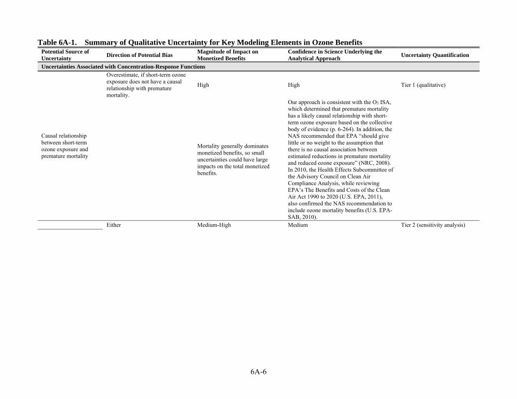
6A-6
Table 6A-1. Summary of Qualitative Uncertainty for Key Modeling Elements in Ozone Benefits Potential Source of Uncertainty
Direction of Potential Bias Magnitude of Impact on Monetized Benefits
Confidence in Science Underlying the Analytical Approach
Uncertainty Quantification
Uncertainties Associated with Concentration-Response Functions
Causal relationship between short-term ozone exposure and premature mortality
Overestimate, if short-term ozone exposure does not have a causal relationship with premature mortality.
High High Tier 1 (qualitative)
Mortality generally dominates monetized benefits, so small uncertainties could have large impacts on the total monetized benefits.
Our approach is consistent with the O3 ISA, which determined that premature mortality has a likely causal relationship with short-term ozone exposure based on the collective body of evidence (p. 6-264). In addition, the NAS recommended that EPA “should give little or no weight to the assumption that there is no causal association between estimated reductions in premature mortality and reduced ozone exposure” (NRC, 2008). In 2010, the Health Effects Subcommittee of the Advisory Council on Clean Air Compliance Analysis, while reviewing EPA’s The Benefits and Costs of the Clean Air Act 1990 to 2020 (U.S. EPA, 2011), also confirmed the NAS recommendation to include ozone mortality benefits (U.S. EPA-SAB, 2010).
Either Medium-High Medium Tier 2 (sensitivity analysis)

6A-7
Potential Source of Uncertainty
Direction of Potential Bias Magnitude of Impact on Monetized Benefits
Confidence in Science Underlying the Analytical Approach
Uncertainty Quantification
Shape of the C-R functions, particularly at low concentrations for short-term ozone exposure-related mortality
The direction of bias that assuming a linear-no threshold model or alternative model introduces depends upon the “true” functional from of the relationship and the specific assumptions and data in a particular analysis. For example, if the true function identifies a threshold below which health effects do not occur, benefits may be overestimated if a substantial portion of those benefits were estimated to occur below that threshold. Alternately, if a substantial portion of the benefits occurred above that threshold, the benefits may be underestimated because an assumed linear no-threshold function may not reflect the steeper slope above that threshold to account for all health effects occurring above that threshold.
The magnitude of this impact depends on the fraction of benefits occurring in areas with lower concentrations. Mortality generally dominates monetized benefits, so small uncertainties could have large impacts on total monetized benefits.
The O3 ISA did not find any evidence that supports a threshold in the relationship between short-term exposure to ozone and mortality within the range of ozone concentrations observed in the U.S., and recent evidence suggests that the shape of the ozone-mortality C-R curve remains linear across the full range of ozone concentrations (p. 6-257). Consistent with the O3 ISA, we assume a log-linear no-threshold model for the C-R functions for short-term ozone mortality. However, the ISA notes that there is less certainty in the shape of the C-R function below 20 ppb due to the low density of data in this range (p. 6-254-255).
The comparison of short-term mortality against the associated distribution of (ozone season-averaged) 8-hour maximum ozone concentrations (see Appendix 6B, section 6B.7) suggests that the vast majority of predicted reductions in mortality are associated with days having 8-hour maximum concentrations that fall within the higher confidence range.
Causal relationship between long-term ozone exposure and premature respiratory mortality
Overestimate, if long-term ozone exposure does not have a causal relationship with premature mortality.
Potentially High, if included in monetized benefits
Medium Tier 1 (qualitative)
Mortality generally dominates monetized benefits, so small uncertainties could have large impacts on the total monetized benefits. However, we have not included long-term ozone mortality in the monetized benefits for this analysis due to uncertainties in the cessation lag.
While the O3 ISA concludes that evidence is suggestive of a causal association between total mortality and long-term ozone exposure (section 7.7.1), specifically with regard to respiratory health effects (including mortality), the ISA concludes that there is likely to be a causal association (section 7.2.8).
Shape of the C-R functions, particularly at low concentrations for long-term ozone exposure-related respiratory mortality
Either Potentially High, if included in monetized benefits
Medium Tier 2 (sensitivity analysis)
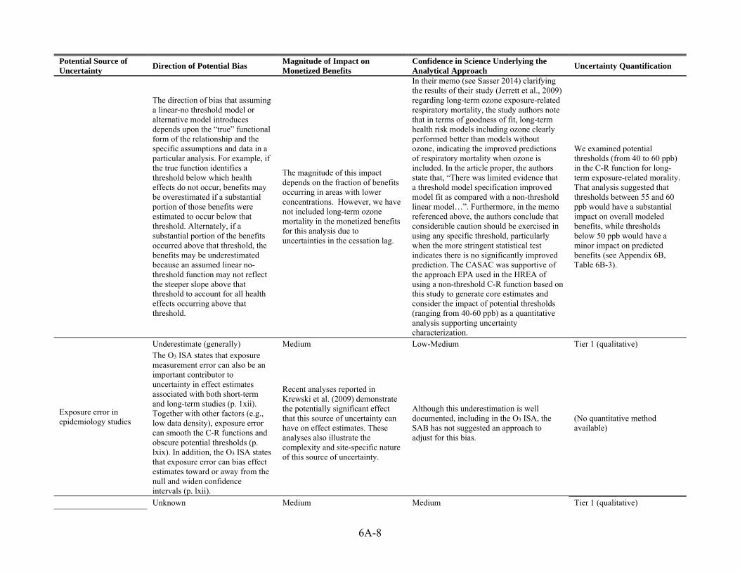
6A-8
Potential Source of Uncertainty
Direction of Potential Bias Magnitude of Impact on Monetized Benefits
Confidence in Science Underlying the Analytical Approach
Uncertainty Quantification
The direction of bias that assuming a linear-no threshold model or alternative model introduces depends upon the “true” functional form of the relationship and the specific assumptions and data in a particular analysis. For example, if the true function identifies a threshold below which health effects do not occur, benefits may be overestimated if a substantial portion of those benefits were estimated to occur below that threshold. Alternately, if a substantial portion of the benefits occurred above that threshold, the benefits may be underestimated because an assumed linear no-threshold function may not reflect the steeper slope above that threshold to account for all health effects occurring above that threshold.
The magnitude of this impact depends on the fraction of benefits occurring in areas with lower concentrations. However, we have not included long-term ozone mortality in the monetized benefits for this analysis due to uncertainties in the cessation lag.
In their memo (see Sasser 2014) clarifying the results of their study (Jerrett et al., 2009) regarding long-term ozone exposure-related respiratory mortality, the study authors note that in terms of goodness of fit, long-term health risk models including ozone clearly performed better than models without ozone, indicating the improved predictions of respiratory mortality when ozone is included. In the article proper, the authors state that, “There was limited evidence that a threshold model specification improved model fit as compared with a non-threshold linear model…”. Furthermore, in the memo referenced above, the authors conclude that considerable caution should be exercised in using any specific threshold, particularly when the more stringent statistical test indicates there is no significantly improved prediction. The CASAC was supportive of the approach EPA used in the HREA of using a non-threshold C-R function based on this study to generate core estimates and consider the impact of potential thresholds (ranging from 40-60 ppb) as a quantitative analysis supporting uncertainty characterization.
We examined potential thresholds (from 40 to 60 ppb) in the C-R function for long-term exposure-related morality. That analysis suggested that thresholds between 55 and 60 ppb would have a substantial impact on overall modeled benefits, while thresholds below 50 ppb would have a minor impact on predicted benefits (see Appendix 6B, Table 6B-3).
Exposure error in epidemiology studies
Underestimate (generally) Medium Low-Medium Tier 1 (qualitative) The O3 ISA states that exposure measurement error can also be an important contributor to uncertainty in effect estimates associated with both short-term and long-term studies (p. 1xii). Together with other factors (e.g., low data density), exposure error can smooth the C-R functions and obscure potential thresholds (p. lxix). In addition, the O3 ISA states that exposure error can bias effect estimates toward or away from the null and widen confidence intervals (p. lxii).
Recent analyses reported in Krewski et al. (2009) demonstrate the potentially significant effect that this source of uncertainty can have on effect estimates. These analyses also illustrate the complexity and site-specific nature of this source of uncertainty.
Although this underestimation is well documented, including in the O3 ISA, the SAB has not suggested an approach to adjust for this bias.
(No quantitative method available)
Unknown Medium Medium Tier 1 (qualitative)

6A-9
Potential Source of Uncertainty
Direction of Potential Bias Magnitude of Impact on Monetized Benefits
Confidence in Science Underlying the Analytical Approach
Uncertainty Quantification
Adjustment of risk coefficients to 8-hour maximum from 24-hour average or 1-hour maximum in the epidemiology studies
We converted these metrics to maximum 8-hour average ozone concentration using standard conversion functions based on observed relationships in the underlying studies. If the relationships between air metrics reported in the studies differ systematically from the relationships seen across the modeling domain, then bias could be introduced.
This conversion does not affect the relative magnitude of the health impact function. However, the pattern of 8-hour maximum concentrations for a particular location over an ozone season could differ from the pattern of 1-hour max or 24-hour average metrics for that same location. Consequently, monetized benefits could differ for a particular location depending on the metric used in modeling benefits.
This practice is consistent both with the available exposure modeling and with the form of the current ozone standard. However, in some cases, these conversions were not specific to the ozone “warm” season, which introduces additional uncertainty due to the use of effect estimates based on a mixture of warm season and all year data in the epidemiological studies.
(No quantitative method available)
Confounding by individual risk factors, other than socioeconomic status—e.g., smoking, or ecologic factors, which represent the neighborhood, such as unemployment
Either, depending on the factor and study
Medium Medium Tier 2 (sensitivity analysis)
Individual, social, economic, and demographic covariates can bias the relationship between particulate air pollution and mortality, particularly in cohort studies that rely on regional air pollution levels.
Because mortality dominates monetized benefits, even a small amount of confounding could have medium impacts on total monetized benefits.
To minimize confounding effects, we use risk coefficients that control for individual risk factors to the extent practical.
(Quantitative methods available but not assessed in this analysis.)
Confounding and effect modification by co-pollutants
Either, depending upon the pollutant.
Medium Medium Tier 1 (qualitative)
Disentangling the health responses of combustion-related pollutants (i.e., PM, SOx, NOx, ozone, and CO) is a challenge. The PM ISA states that co-pollutants may mediate the effects of PM or PM may influence the toxicity of co-pollutants (U.S. EPA, 2009, p. 1–16). Alternately, effects attributed to one pollutants may be due to another.
Because this uncertainty could affect mortality and because mortality generally dominates monetized benefits, even small uncertainties could have medium impacts on total monetized benefits.
The O3 ISA states that there is high confidence that unmeasured confounders are not producing the findings when multiple studies are conducted in various settings using different subjects or exposures, such as multi-city studies (p. lxi). When modeling effects of pollutants jointly (e.g., PM and O3), we apply multi-pollutant effect estimates when those estimates are available to avoid double-counting and satisfy other selection criteria. In addition, we apply multi-city effect estimates when available.
(No quantitative method available)
Application of C-R relationships only to the original study population
Underestimate Low High Tier 2 (sensitivity analysis)
Estimating health effects for only the original study population may underestimate the whole population benefits of reductions in pollutant exposures.
Mortality generally dominates monetized benefits, so further age range expansions for morbidity endpoints would have a small impact on total monetized benefits.
Following advice from the SAB (U.S. EPA-SAB, 2004a, pg. 7) and NAS (NRC, 2002, pg. 114), we expanded the age range for childhood asthma exacerbations beyond the original study population to ages 6-18.
(Quantitative methods available but not assessed in this analysis.)
Uncertainties Associated with Economic Valuation
Unknown High Medium Tier 3 (probabilistic)
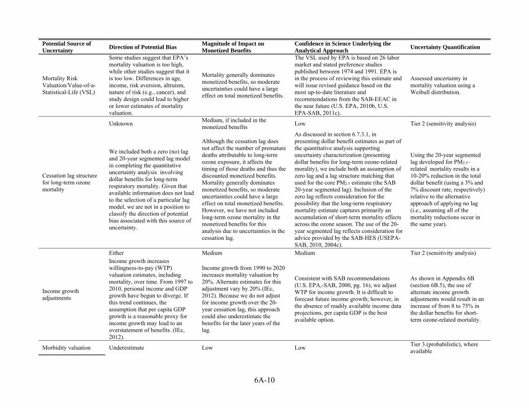
6A-10
Potential Source of Uncertainty
Direction of Potential Bias Magnitude of Impact on Monetized Benefits
Confidence in Science Underlying the Analytical Approach
Uncertainty Quantification
Mortality Risk Valuation/Value-of-a-Statistical-Life (VSL)
Some studies suggest that EPA’s mortality valuation is too high, while other studies suggest that it is too low. Differences in age, income, risk aversion, altruism, nature of risk (e.g., cancer), and study design could lead to higher or lower estimates of mortality valuation.
Mortality generally dominates monetized benefits, so moderate uncertainties could have a large effect on total monetized benefits.
The VSL used by EPA is based on 26 labor market and stated preference studies published between 1974 and 1991. EPA is in the process of reviewing this estimate and will issue revised guidance based on the most up-to-date literature and recommendations from the SAB-EEAC in the near future (U.S. EPA, 2010b, U.S. EPA-SAB, 2011c).
Assessed uncertainty in mortality valuation using a Weibull distribution.
Cessation lag structure for long-term ozone mortality
Unknown Medium, if included in the monetized benefits
Low Tier 2 (sensitivity analysis)
We included both a zero (no) lag and 20-year segmented lag model in completing the quantitative uncertainty analysis involving dollar benefits for long-term respiratory mortality. Given that available information does not lead to the selection of a particular lag model, we are not in a position to classify the direction of potential bias associated with this source of uncertainty.
Although the cessation lag does not affect the number of premature deaths attributable to long-term ozone exposure, it affects the timing of those deaths and thus the discounted monetized benefits. Mortality generally dominates monetized benefits, so moderate uncertainties could have a large effect on total monetized benefits. However, we have not included long-term ozone mortality in the monetized benefits for this analysis due to uncertainties in the cessation lag.
As discussed in section 6.7.3.1, in presenting dollar benefit estimates as part of the quantitative analysis supporting uncertainty characterization (presenting dollar benefits for long-term ozone-related morality), we include both an assumption of zero lag and a lag structure matching that used for the core PM2.5 estimate (the SAB 20-year segmented lag). Inclusion of the zero lag reflects consideration for the possibility that the long-term respiratory mortality estimate captures primarily an accumulation of short-term mortality effects across the ozone season. The use of the 20-year segmented lag reflects consideration for advice provided by the SAB-HES (USEPA-SAB, 2010, 2004c).
Using the 20-year segmented lag developed for PM2.5–related mortality results in a 10-20% reduction in the total dollar benefit (using a 3% and 7% discount rate, respectively) relative to the alternative approach of applying no lag (i.e., assuming all of the mortality reductions occur in the same year).
Income growth adjustments
Either Medium Medium Tier 2 (sensitivity analysis) Income growth increases willingness-to-pay (WTP) valuation estimates, including mortality, over time. From 1997 to 2010, personal income and GDP growth have begun to diverge. If this trend continues, the assumption that per capita GDP growth is a reasonable proxy for income growth may lead to an overstatement of benefits. (IEc, 2012).
Income growth from 1990 to 2020 increases mortality valuation by 20%. Alternate estimates for this adjustment vary by 20% (IEc, 2012). Because we do not adjust for income growth over the 20-year cessation lag, this approach could also underestimate the benefits for the later years of the lag.
Consistent with SAB recommendations (U.S. EPA,-SAB, 2000, pg. 16), we adjust WTP for income growth. It is difficult to forecast future income growth; however, in the absence of readily available income data projections, per capita GDP is the best available option.
As shown in Appendix 6B (section 6B.5), the use of alternate income growth adjustments would result in an increase of from 8 to 75% in the dollar benefits for short-term ozone-related mortality.
Morbidity valuation Underestimate Low Low Tier 3 (probabilistic), where available

6A-11
Potential Source of Uncertainty
Direction of Potential Bias Magnitude of Impact on Monetized Benefits
Confidence in Science Underlying the Analytical Approach
Uncertainty Quantification
Morbidity benefits such as hospital admissions are calculated using cost-of-illness (COI) estimates, which are generally half the WTP to avoid the illness (Alberini and Krupnick, 2000). In addition, the morbidity costs do not reflect physiological responses or sequelae events, such as increased susceptibility for future morbidity.
Even if we doubled the monetized valuation of morbidity endpoints using COI valuations that are currently included in the RIA, the change would still be less than 5% of the monetized benefits. It is unknown how much including sequelae events could increase morbidity valuation.
Although the COI estimates for hospitalizations reflect recent data, we have not yet updated other COI estimates such as for school loss days. The SAB concluded that COI estimates could be used as placeholders where WTP estimates are unavailable, but it is reasonable to presume that this strategy typically understates WTP values (U.S. EPA-SAB, 2004b, pg. 3).
Assessed uncertainty in morbidity valuation using distributions specified in the underlying literature, where available (see Table 6-10).
Uncertainties Associated with Baseline Incidence and Population Projections
Population estimates and projections
Either Low–Medium Medium Tier 1 (qualitative)
The monetized benefits would change in the same direction as the over- or underestimate in population projections in areas where exposure changes.
Monetized benefits are substantially affected by population density. Comparisons using historical Census data show that population projections are ±5% nationally, but projection accuracy can vary by locality. Historical error for Woods & Poole’s population projections has been ±8.1% for county-level projections and ±4.1% for states (Woods and Poole, 2012). The magnitude of impact on total monetized benefits depends on the specific location where ozone is reduced.
We use population projections for 5-year increments for 304 race/ethnicity/gender/age groups (Woods and Poole, 2012) at Census blocks. Population forecasting is well-established but projections of future migration due to possible catastrophic events are not considered. In addition, projections at the small spatial scales used in this analysis are inherently more uncertain than projections at the county- or state-level.
(No quantitative method available)
Uncertainty in projecting baseline incidence rates for mortality
Unknown Low-Medium Medium Tier 1 (qualitative)
Because the mortality rate projections for future years reflect changes in mortality patterns as well as population growth, the projections are unlikely to be biased.
Because mortality generally dominates monetized benefits, small uncertainties could have medium impacts on total monetized benefits.
The county-level baseline mortality rates reflect recent databases (i.e., 2004–2006 data) and are projected for 5-year increments for multiple age groups. This database is generally considered to have relatively low uncertainty (CDC Wonder, 2008). The projections account for both spatial and temporal changes in the population.
(No quantitative method available)
Uncertainty in projecting baseline
Either, depending on the health endpoint
Low Low-Medium Tier 1 (qualitative)

6A-12
Potential Source of Uncertainty
Direction of Potential Bias Magnitude of Impact on Monetized Benefits
Confidence in Science Underlying the Analytical Approach
Uncertainty Quantification
incidence rates and prevalence rates for morbidity
Morbidity baseline incidence is available for current year only (i.e., no projections available). Assuming current year levels can bias the benefits for a specific endpoint if the data has clear trends over time. Specifically, asthma prevalence rates have increased substantially over the past few years while hospital admissions have decreased substantially.
The magnitude varies with the health endpoint, but the overall impact on the total benefits estimate from these morbidity endpoints is likely to be low.
We do not have a method to project future baseline morbidity rates, thus we assume current year levels will continue. While we try to update the baseline incidence and prevalence rates as frequently as practicable, this does not continue trends into the future. Some endpoints, such as hospitalizations and ER visits, have more recent data (i.e., 2007) stratified by age and geographic location. Other endpoints, such as respiratory symptoms, reflect a national average. Asthma prevalence rates reflect recent increases in baseline asthma rates (i.e., 2008).
(No quantitative method available)
Uncertainties Associated with Omitted Benefits Categories
Unquantified ozone health benefit categories, such as worker productivity and long-term mortality
Underestimate High Low Tier 2 (sensitivity analysis)
EPA has not included monetized estimates of these benefits categories in the core benefits estimate.
Although the potential magnitude is unknown, including all of the additional endpoints associated with ozone exposure that are currently not monetized could increase the total benefits by a large amount.
Current data and methods are insufficient to value national quantitative estimates of these health effects. The O3 ISA determined that respiratory effects (including mortality) are causally associated with long-term ozone exposure (p. 2–17). The O3 ISA also determined that outdoor workers have an increased risk of ozone-related health effects (p. 1-15), and that studies on outdoor workers show consistent evidence that short-term increases in ambient ozone exposure can decrease lung function in healthy adults (p.6-38). Additional studies link short-term ozone exposure to reduced productivity in outdoor workers (Graf Zivin and Neidell, 2013; Crocker and Horst, 1981).
We include a quantitative uncertainty analysis reflecting long-term mortality, which shows that this endpoint could add substantially to the monetized benefits (see Appendix 6B, section 6B.2). We have also included a analysis reflecting application of an updated worker productivity analysis (see section 6.5.3).
Uncertainties Associated with Estimated Exposure Changes
Spatial matching of air quality estimates from epidemiology studies to air quality estimates from air quality modeling
Unknown Unknown Low Tier 1 (qualitative) Epidemiology studies often assume one air quality concentration is representative of an entire urban area when calculating hazard ratios, while benefits are calculated using air quality modeling conducted at 12 km spatial resolution. This spatial mismatch could introduce uncertainty.
We have not controlled for this potential bias, and the SAB has not suggested an approach to adjust for this bias.
(No quantitative method available)
6A-13
6A.3 References
Alberini, Anna and Alan Krupnick. 2000. “Cost-of-Illness and Willingness-to-Pay Estimates of the Benefits of Improved Air Quality: Evidence from Taiwan.” Land Economics Vol. 76, No. 1 (Feb), pp. 37-53.
Centers for Disease Control and Prevention (CDC). 2008. National Center for Health Statistics. National Health Interview Survey, 1999-2008.
Crocker, T. D., & Horst, R. L. (1981). Hours of work, labor productivity, and environmental conditions: A case study. The Review of Economics and Statistics, 63(3), 361-368.
Fann, N.; K.R. Baker and C.M. Fulcher. 2012. “Characterizing the PM2.5-related health benefits of emission reductions for 17 industrial, area and mobile emission sectors across the U.S.” Environment International 49 41–151.
Graff Zivin, J., Neidell, M. (2012). “The impact of pollution on worker productivity.” American Economic Review, 102, 3652-3673.
Industrial Economics, Incorporated (IEc). 2012. Updating BenMAP Income Elasticity Estimates—Literature Review. Memo to Neal Fann. March. Available on the Internet at <http://www.epa.gov/ttn/ecas/regdata/Benefits/Income%20Elasticity%20Update_Recommendations_noAppD.pdf>
Jerrett M, Burnett RT, Pope CA, III, et al. 2009. “Long-Term Ozone Exposure and Mortality.” New England Journal of Medicine 360:1085-95.
Krewski D, Jerrett M, Burnett RT, Ma R, Hughes E, Shi, Y, et al. 2009. “Extended follow-up and spatial analysis of the American Cancer Society study linking particulate air pollution and mortality.” HEI Research Report, 140, Health Effects Institute, Boston, MA.
Mansfield, Carol; Paramita Sinha; Max Henrion. 2009. Influence Analysis in Support of Characterizing Uncertainty in Human Health Benefits Analysis: Final Report. Prepared for U.S. EPA, Office of Air Quality Planning and Standards. November. Available on the internet at <http://www.epa.gov/ttn/ecas/regdata/Benefits/influence_analysis_final_report_psg.pdf>.
National Research Council (NRC). 2002. Estimating the Public Health Benefits of Proposed Air Pollution Regulations. Washington, DC: The National Academies Press. Washington, DC.
National Research Council (NRC). 2008. Estimating Mortality Risk Reduction and Economic Benefits from Controlling Ozone Air Pollution. National Academies Press. Washington, DC.
Sasser, E. 2014. Response to Comments Regarding the Potential Use of a Threshold Model in Estimating the Mortality Risks from Long-term Exposure to Ozone in the Health Risk and Exposure Assessment for Ozone, Second External Review Draft. Memorandum to Holly Stallworth, Designated Federal Officer, Clean Air Scientific Advisory Committee from EPA/OAQPS Health and Environmental Impacts Division.
U.S. Environmental Protection Agency (U.S. EPA). 2001. Risk assessment guidance for Superfund. Vol. III, Part A. Process for conducting probabilistic risk assessment (RAGS 3A). Washington, DC, United States Environmental Protection Agency (EPA 540-R-02-002; OSWER 9285.7-45; PB2002 963302. Available on the Internet at <http://www.epa.gov/oswer/riskassessment/rags3adt/index.htm>.
U.S. Environmental Protection Agency (U.S. EPA). 2004. EPA’s risk assessment process for air toxics: History and overview. In: Air toxics risk assessment reference library. Vol. 1. Technical resource manual. Washington, DC,

6A-14
United States Environmental Protection Agency, pp. 3-1–3-30 (EPA-453-K-04-001A. Available on the Internet at <http://www.epa.gov/ttn/fera/data/risk/vol_1/chapter_03.pdf>.
U.S. Environmental Protection Agency (U.S. EPA). 2009. Integrated Science Assessment for Particulate Matter (Final Report). EPA-600-R-08-139F. National Center for Environmental Assessment—RTP Division. December. Available at <http://cfpub.epa.gov/ncea/cfm/recordisplay.cfm?deid=216546>.
U.S. Environmental Protection Agency (U.S. EPA). 2010a. Quantitative Health Risk Assessment for Particulate Matter—Final Report. EPA-452/R-10-005. Office of Air Quality Planning and Standards, Research Triangle Park, NC. September. Available on the Internet at <http://www.epa.gov/ttnnaaqs/standards/pm/data/PM_RA_FINAL_June_2010.pdf>.
U.S. Environmental Protection Agency (U.S. EPA). 2010b. Valuing Mortality Risk Reductions for Environmental Policy: A White Paper (SAB Review Draft). December. Available on the Internet at <http://yosemite.epa.gov/ee/epa/eerm.nsf/vwAN/EE-0563-1.pdf/$file/EE-0563-1.pdf>.
U.S. Environmental Protection Agency (U.S. EPA). 2011. The Benefits and Costs of the Clean Air Act 1990 to 2020: EPA Report to Congress. Office of Air and Radiation, Office of Policy, Washington, DC. March. Available on the Internet at <http://www.epa.gov/oar/sect812/feb11/fullreport.pdf>.
U.S. Environmental Protection Agency (U.S. EPA). 2012. Regulatory Impact Analysis for the Final Revisions to the National Ambient Air Quality Standards for Particulate Matter. EPA-452/R-12-003. Office of Air Quality Planning and Standards, Health and Environmental Impacts Division. December. Available at: <http://www.epa.gov/pm/2012/finalria.pdf>.
U.S. Environmental Protection Agency (U.S. EPA). 2013. Integrated Science Assessment of Ozone and Related Photochemical Oxidants (Final Report). U.S. Environmental Protection Agency, Washington, DC, EPA/600/R-10/076F. Available at: <http://cfpub.epa.gov/ncea/isa/recordisplay.cfm?deid=247492#Download>.
U.S. Environmental Protection Agency (U.S. EPA). 2014. Health Risk and Exposure Assessment for Ozone Final Report. EPA-452/R-14-004a. Office of Air Quality Planning and Standards, Health and Environmental Impacts Division. August. Available at: < http://www.epa.gov/ttn/naaqs/standards/ozone/data/20140829healthrea.pdf>.
U.S. Environmental Protection Agency—Science Advisory Board (U.S. EPA-SAB). 1999. An SAB Advisory: The Clean Air Act Section 812 Prospective Study Health and Ecological Initial Studies. EPA-SAB-COUNCIL-ADV-99-005, Available on the Internet at <http://yosemite.epa.gov/sab/sabproduct.nsf/1AFDEBB45C57F6E5852571930058C1A5/$File/coua9905.pdf>.
U.S. Environmental Protection Agency—Science Advisory Board (U.S. EPA-SAB). 2000. The Clean Air Act Amendments (CAAA) Section 812 Prospective Study of Costs and Benefits (1999): Advisory by the Advisory Council on Clean Air Compliance Analysis: Costs and Benefits of the CAAA. EPA-SAB-COUNCIL-ADV-00-002. October. Available on the Internet at <http://yosemite.epa.gov/sab/sabproduct.nsf/E992F918DF32131A852571B9004571F7/$File/coua0002.pdf>.
U.S. Environmental Protection Agency—Science Advisory Board (U.S. EPA-SAB). 2001. REVIEW OF THE DRAFT ANALYTICAL PLAN FOR EPA’S SECOND PROSPECTIVE ANALYSIS - BENEFITS AND COSTS OF THE CLEAN AIR ACT 1990- 2020. EPA-SAB-COUNCIL-ADV-01-004, Available on the Internet at <http://yosemite.epa.gov/sab/sabproduct.nsf/572DC1989A3986CC8525718D006BAB8B/$File/councila01004.pdf>.
U.S. Environmental Protection Agency—Science Advisory Board (U.S. EPA-SAB). 2004a. Advisory on Plans for Health Effects Analysis in the Analytical Plan for EPA’s Second Prospective Analysis—Benefits and Costs of the Clean Air Act, 1990–2020. EPA-SAB-COUNCIL-ADV-04-002. March. Available on the Internet at

6A-15
<http://yosemite.epa.gov/sab%5CSABPRODUCT.NSF/08E1155AD24F871C85256E5400433D5D/$File/council_adv_04002.pdf>.
U.S. Environmental Protection Agency—Science Advisory Board (U.S. EPA-SAB). 2004b. Review of the Draft Analytical Plan for EPA’s Second Prospective Analysis—Benefits and Costs of the Clean Air Act, 1990-2020: An Advisory by the Advisory Council for Clean Air Compliance Analysis. EPA-SAB-COUNCIL-ADV-04-004. May. Available on the Internet at <http://yosemite.epa.gov/sab/sabproduct.nsf/7CCBBFE15CD4C8B185256F17005E3079/$File/council_adv_04004.pdf>.
U.S. Environmental Protection Agency—Science Advisory Board (U.S. EPA-SAB). 2004c. Advisory Council on Clean Air Compliance Analysis Response to Agency Request on Cessation Lag. EPA-COUNCIL-LTR-05-001. December. Available on the Internet at <http://yosemite.epa.gov/sab/sabproduct.nsf/0/39F44B098DB49F3C85257170005293E0/$File/council_ltr_05_001.pdf>.
U.S. Environmental Protection Agency—Science Advisory Board (U.S. EPA-SAB). 2010. Review of EPA’s DRAFT Health Benefits of the Second Section 812 Prospective Study of the Clean Air Act. EPA-COUNCIL-10-001. June. Available on the Internet at <http://yosemite.epa.gov/sab/sabproduct.nsf/9288428b8eeea4c885257242006935a3/72D4EFA39E48CDB28525774500738776/$File/EPA-COUNCIL-10-001-unsigned.pdf>.
U.S. Environmental Protection Agency—Science Advisory Board (U.S. EPA-SAB). 2011a. CASAC Review of Quantitative Health Risk Assessment for Particulate Matter—Second External Review Draft (February 2010). EPA-CASAC-10-008. Available on the Internet at <http://yosemite.epa.gov/sab/sabproduct.nsf/BC4F6E77B6385155852577070002F09F/$File/EPA-CASAC-10-008-unsigned.pdf>.
U.S. Environmental Protection Agency—Science Advisory Board (U.S. EPA-SAB). 2011b. Review of the Final Integrated Report for the Second Section 812 Prospective Study of the Benefits and Costs of the Clean Air Act (August 2010). EPA-COUNCIL-11-001. Available on the Internet at <http://yosemite.epa.gov/sab/sabproduct.nsf/1E6218DE3BFF682E852577FB005D46F1/$File/EPA-COUNCIL-11-001-unsigned.pdf>.
U.S. Environmental Protection Agency—Science Advisory Board (U.S. EPA-SAB). 2011c. Review of Valuing Mortality Risk Reductions for Environmental Policy: A White Paper (December 10, 2010). EPA-SAB-11-011. July. Available on the Internet at <http://yosemite.epa.gov/sab/sabproduct.nsf/298E1F50F844BC23852578DC0059A616/$File/EPA-SAB-11-011-unsigned.pdf>.
Woods & Poole Economics, Inc. 2012. Complete Economic and Demographic Data Source (CEDDS). CD-ROM. Woods & Poole Economics, Inc. Washington, D.C.
World Health Organization (WHO). 2008. Part 1: Guidance Document on Characterizing and Communicating Uncertainty in Exposure Assessment, Harmonization Project Document No. 6. Published under joint sponsorship of the World Health Organization, the International Labour Organization and the United Nations Environment Programme. WHO Press: Geneva, Switzerland. Available on the Internet at <www.who.int/ipcs/methods/harmonization/areas/uncertainty%20.pdf>.

6B-1
APPENDIX 6B: QUANTITATIVE ANALYSES COMPLETED IN SUPPORT OF UNCERTAINTY CHARACTERIZATION
Overview
The benefits analysis presented in Chapter 6 of this RIA is based on our current
interpretation of the scientific and economic literature. That interpretation requires judgments
regarding the best available data, models, and analytical methodologies and the assumptions that
are most appropriate to adopt in the face of important uncertainties. The majority of the
analytical assumptions used to develop the main estimates of benefits have been reviewed and
supported by EPA’s independent Science Advisory Board (SAB). Both EPA and the SAB
recognize that data and modeling limitations, as well as simplifying assumptions can introduce
uncertainty into the estimates of benefits and that alternative choices exist for some inputs to the
analysis, such as the concentration-response (C-R) functions for mortality.
This appendix presents a set of quantitative analysis completed in support of uncertainty
characterization including exploration of: (a) alternative studies in modeling short-term ozone
exposure-related mortality (section 6B.1), (b) monetized benefits associated with mortality
resulting from long-term exposure to ozone (section 6B.2), (c) the potential impact of thresholds
in long-term ozone exposure-related mortality in incidence and benefits estimates (section 6B.3),
(d) alternative response functions developed through expert elicitation for long-term PM2.5
exposure-related mortality (section 6B.4), (e) alternative assumptions regarding income elasticity
on benefits derived using willingness-to-pay (WTP) functions (section 6B.5), (f) age group-
differentiated aspects of short-term ozone exposure-related mortality (including total avoided
incidence, life years gained and percent reduction in baseline mortality - Section 6B.6), (g)
mortality impacts relative to the baseline pollutant concentrations (used in generating those
mortality estimates) for both short-term ozone exposure-related mortality and long-term PM2.5
exposure-related mortality (Section 6B.7) and (h) ozone-related impacts on outdoor worker
productivity (including a detailed discussion of the methodology used in modeling and
presentation of results, Section 6B.8).
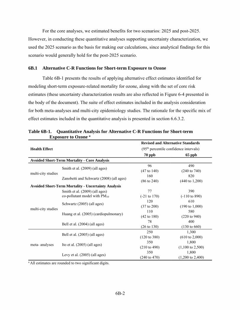
6B-2
For the core analyses, we estimated benefits for two scenarios: 2025 and post-2025.
However, in conducting these quantitative analyses supporting uncertainty characterization, we
used the 2025 scenario as the basis for making our calculations, since analytical findings for this
scenario would generally hold for the post-2025 scenario.
6B.1 Alternative C-R Functions for Short-term Exposure to Ozone
Table 6B-1 presents the results of applying alternative effect estimates identified for
modeling short-term exposure-related mortality for ozone, along with the set of core risk
estimates (these uncertainty characterization results are also reflected in Figure 6-4 presented in
the body of the document). The suite of effect estimates included in the analysis consideration
for both meta-analyses and multi-city epidemiology studies. The rationale for the specific mix of
effect estimates included in the quantitative analysis is presented in section 6.6.3.2.
Table 6B-1. Quantitative Analysis for Alternative C-R Functions for Short-term Exposure to Ozone a
Health Effect
Revised and Alternative Standards
(95th percentile confidence intervals)
70 ppb 65 ppb
Avoided Short-Term Mortality - Core Analysis
multi-city studies Smith et al. (2009) (all ages)
96 490 (47 to 140) (240 to 740)
Zanobetti and Schwartz (2008) (all ages) 160 820
(86 to 240) (440 to 1,200) Avoided Short-Term Mortality - Uncertainty Analysis
multi-city studies
Smith et al. (2009) (all ages) co-pollutant model with PM10
77 390 (-21 to 170) (-110 to 890)
Schwartz (2005) (all ages) 120 610
(37 to 200) (190 to 1,000)
Huang et al. (2005) (cardiopulmonary) 110 580
(42 to 180) (220 to 940)
Bell et al. (2004) (all ages) 78 400
(26 to 130) (130 to 660)
meta- analyses
Bell et al. (2005) (all ages) 250 1,300
(120 to 380) (610 to 2,000)
Ito et al. (2005) (all ages) 350 1,800
(210 to 490) (1,100 to 2,500)
Levy et al. (2005) (all ages) 350 1,800
(240 to 470) (1,200 to 2,400) a All estimates are rounded to two significant digits.

6B-3
This quantitative analysis showed that the two core incidence estimates fall within (and
towards the lower end of) the broader range resulting from application of the seven alternative
effect estimates (note that these observations based on incidence would also hold for the
matching set of dollar benefit estimates generated for this endpoint category).
6B.2 Monetized Benefits for Premature Mortality from Long-term Exposure to Ozone
As discussed in section 6.3, due to uncertainty in specifying the temporal lag structure
associated with reductions in long-term ozone-related respiratory mortality, we have included
these estimates as an uncertainty analysis and not as part of the core dollar benefit estimate.
Table 6B-2 presents the dollar benefits (2011$) associated with modeled reductions in long-term
ozone-related respiratory mortality. These benefit estimates are generated using non-threshold
models obtained from Jerrett et al. (2009) because we present the potential threshold analysis in
the section 6B.3. Additional detail on the effect estimates used in the core analysis and this
uncertainty analysis is presented in section 6.6.3.2. Section 6.6.4 provides additional detail on
the approach used in valuing these mortality estimates including how uncertainty related to
cessation lag was addressed.
Table 6B-2. Monetized Benefits for Mortality from Long-term Exposure to Ozone (millions of 2011$) (2025 and post-2025 scenarios)a, d
70 ppb 65 ppb
Avoided Long-term Respiratory Mortality
2025 scenario
$3,400 $17,000
($280 to $10,000) ($1,400 to $52,000)
$2,800 to $3,100 $14,000 to $16,000
($250 to $8,400) ($1,200 to $47,000)
post-2025 scenario
$3,000 $6,000
($240 to $8,400) ($490 to $18,000)
$2,400 to $2,700 $4,900 to $5,400
($200 to $8,000) ($400 to $18,000)
Revised and Alterative Standard Levels
(95th percentile confidence intervals)
multi-city study
Jerrett et al. (2009) (age 30-99)
copollutants model (PM2.5) no lag b
multi-city study
Jerrett et al. (2009) (age 30-99)
copollutants model (PM2.5) no lag b
Jerrett et al. (2009) (age 30-99)
copollutants model (PM2.5) 20 yr
segmented lag c
Jerrett et al. (2009) (age 30-99)
copollutants model (PM2.5) 20 yr
segmented lag c
Health Effectb
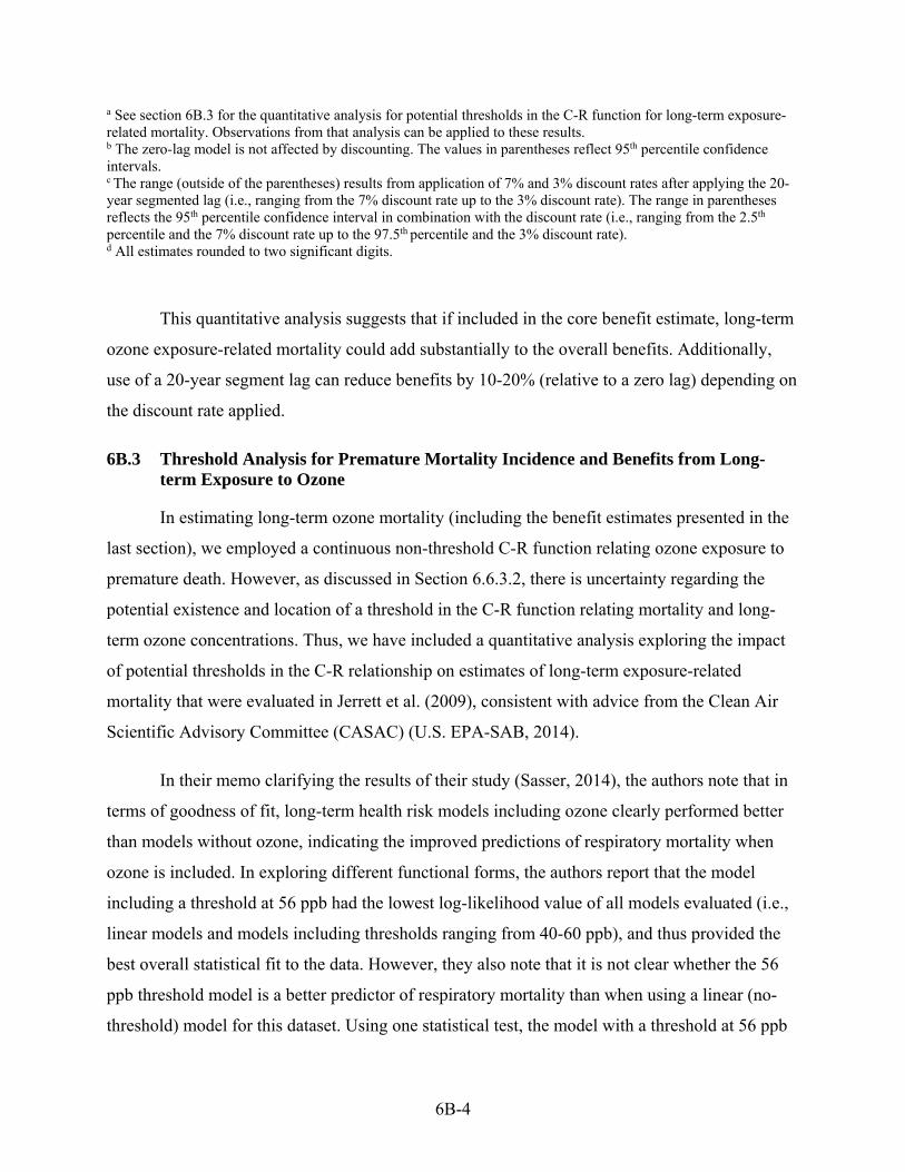
6B-4
a See section 6B.3 for the quantitative analysis for potential thresholds in the C-R function for long-term exposure-related mortality. Observations from that analysis can be applied to these results. b The zero-lag model is not affected by discounting. The values in parentheses reflect 95th percentile confidence intervals. c The range (outside of the parentheses) results from application of 7% and 3% discount rates after applying the 20-year segmented lag (i.e., ranging from the 7% discount rate up to the 3% discount rate). The range in parentheses reflects the 95th percentile confidence interval in combination with the discount rate (i.e., ranging from the 2.5th
percentile and the 7% discount rate up to the 97.5th percentile and the 3% discount rate). d All estimates rounded to two significant digits.
This quantitative analysis suggests that if included in the core benefit estimate, long-term
ozone exposure-related mortality could add substantially to the overall benefits. Additionally,
use of a 20-year segment lag can reduce benefits by 10-20% (relative to a zero lag) depending on
the discount rate applied.
6B.3 Threshold Analysis for Premature Mortality Incidence and Benefits from Long-term Exposure to Ozone
In estimating long-term ozone mortality (including the benefit estimates presented in the
last section), we employed a continuous non-threshold C-R function relating ozone exposure to
premature death. However, as discussed in Section 6.6.3.2, there is uncertainty regarding the
potential existence and location of a threshold in the C-R function relating mortality and long-
term ozone concentrations. Thus, we have included a quantitative analysis exploring the impact
of potential thresholds in the C-R relationship on estimates of long-term exposure-related
mortality that were evaluated in Jerrett et al. (2009), consistent with advice from the Clean Air
Scientific Advisory Committee (CASAC) (U.S. EPA-SAB, 2014).
In their memo clarifying the results of their study (Sasser, 2014), the authors note that in
terms of goodness of fit, long-term health risk models including ozone clearly performed better
than models without ozone, indicating the improved predictions of respiratory mortality when
ozone is included. In exploring different functional forms, the authors report that the model
including a threshold at 56 ppb had the lowest log-likelihood value of all models evaluated (i.e.,
linear models and models including thresholds ranging from 40-60 ppb), and thus provided the
best overall statistical fit to the data. However, they also note that it is not clear whether the 56
ppb threshold model is a better predictor of respiratory mortality than when using a linear (no-
threshold) model for this dataset. Using one statistical test, the model with a threshold at 56 ppb

6B-5
was determined to be statistically superior to the linear model. Using another, more stringent test,
none of the threshold models considered were statistically superior to the linear model. Under the
less stringent test, although the threshold model produces a statistically superior prediction than
the linear model, there is uncertainty about the specific location of the threshold, if one exists.
This is because the confidence intervals on the model predictions indicate that a threshold could
exist anywhere from 0 to 60 ppb. The authors conclude that considerable caution should be
exercised in using any specific threshold, particularly when the more stringent statistical test
indicates there is no significantly improved prediction. Based on this additional information from
the authors, we have chosen to reflect the uncertainty about the existence and location of a
potential threshold by estimating mortality attributable to long-term ozone exposures using a
range of threshold-based effect coefficients. Specifically, we estimate long-term ozone mortality
benefits using unique risk coefficients that include a range of thresholds from 40 ppb to 60 ppb
in 5 ppb increments, while also including a model with a threshold equal to 56 ppb, which had
the lowest log-likelihood value for all models examined.169 Table 6B-3 provides the results of
this uncertainty analysis (based on modeling incidence) for 65 ppb and 70 ppb. The same pattern
in terms of relative reductions across thresholds would also hold for the monetized benefit
estimates.
Table 6B-3. Long-term Ozone Mortality Incidence at Various Assumed Thresholds a Threshold Concentration 70 ppb 65 ppb
No threshold 340 1,700 40 ppb 260 1,300 45 ppb 200 910 50 ppb 59 210 55 ppb 6 66 56 ppb 5 60 60 ppb 3 19
a All estimates rounded to two significant digits.
The results of the uncertainty analysis based on the suite of threshold-based risk
coefficients suggest that threshold models can substantially lower estimates of ozone-attributable
long-term mortality. For example, estimated benefits for long-term mortality using a model that
169 There is a separate effect coefficient (and associated standard error) for each of the fitted threshold models
estimated in Jerrett et al. (2009). As a result, the sensitivity of estimated mortality attributable to long-term ozone concentrations is affected by both the assumed threshold level (below which there is no effect of ozone) and the effect coefficient applied to ozone concentrations above the threshold.

6B-6
includes a 55 ppb threshold are approximately 70% less than long-term mortality benefits
estimated using the co-pollutant, non-threshold model. Generally, estimated long-term mortality
benefits are progressively reduced when using models with increasing thresholds, with the
highest threshold considered (60 ppb) removing virtually all of the estimated incidence reduction
and associated benefits.
6B.4 Alternative C-R Functions for PM2.5–Related Mortality
In estimating PM2.5 co-benefits, monetized benefits are driven largely by reductions in
mortality. Therefore, it is particularly important to attempt to characterize the uncertainties
associated with reductions in premature mortality. In addition to the ACS and Six Cities cohort
studies, several recent cohort studies conducted in North America provide evidence for the
relationship between long-term exposure to PM2.5 and the risk of premature death. Many of these
additional cohort studies are described in the PM ISA (U.S. EPA, 2009) and the Provisional
Assessment (U.S. EPA, 2012a).170, Table 6B-4 provides the effect estimates from each of these
cohort studies for all-cause, cardiovascular, cardiopulmonary, and ischemic heart disease (IHD)
mortality, as well as the lowest measured air quality level (LML) and mean concentration in the
study.
We also draw upon the results of the 2006 expert elicitation171 sponsored by the EPA
(Roman et al., 2008; IEc, 2006) to demonstrate the sensitivity of the benefits estimates to 12
expert-defined C-R functions. The PM2.5 expert elicitation and the derivation of C-R functions
from the expert elicitation results are described in detail in the 2006 PM2.5 NAAQS RIA (U.S.
EPA, 2006), the elicitation summary report (IEc, 2006) and Roman et al. (2008), and we
summarize the key attributes of this study relative to the interpretation of the estimates of PM-
related mortality reported here. We describe also how the epidemiological literature has evolved
since the expert elicitation was conducted in 2005 and 2006.
170 It is important to note that the newer studies in the Provisional Assessment are published in peer-reviewed
journals and meet our study selection criteria, but they have not been assessed in the context of an Integrated Science Assessment nor gone through review by the SAB. In addition, only the ACS and Harvard Six Cities’ cohort studies have been recommended by the SAB as appropriate for benefits analysis of national rulemakings.
171 Expert elicitation is a formal, highly-structured and well-documented process whereby expert judgments, usually of multiple experts, are obtained (Ayyub, 2002).

6B-7
Table 6B-4. Summary of Effect Estimates from Recent Cohort Studies in North America Associated with Change in Long-Term Exposure to PM2.5
Study Cohort (age) LML (µg/m3)
Mean (µg/m3)
Hazard Ratios per 10 µg/m3 Change in PM2.5 (95th percentile confidence intervals)
All Causes Cardiovascular Cardiopulmonary IHD Pope et al. (2002)
ACS (age >30)
7.5 18.2 1.06 (1.02–1.11)
1.12 (1.08–1.15)
1.09 (1.03–1.16)
N/A
Laden et al. (2006)
Six Cities (age > 25)
10 16.4 1.16 (1.07–1.26)
1.28 (1.13–1.44)
N/A N/A
Lipfert et al. (2006)a
Veterans (age 39–63)
<14.1 14.3 1.15 (1.05–1.25)
N/A N/A N/A
Miller et al. (2007)b
WHI (age 50–79)
3.4 13.5 N/A 1.76 (1.25–2.47)
N/A 2.21 (1.17–4.16)
Eftim et al. (2008)
Medicare (age > 65)
6 13.6 1.21 (1.15–1.27)
N/A N/A N/A
Zeger et al. (2008)c
Medicare (age > 65)
<9.8 13.2 1.068 (1.049–1.087)
N/A N/A N/A
Krewski et al. (2009)d
ACS (age >30)
5.8 14 1.06 (1.04–1.08)
N/A 1.13 (1.10–1.16)
1.24 (1.19–1.29)
Puett et al. (2009)b
NHS (age 30–55)
5.8 13.9 1.26 (1.02–1.54)
N/A N/A 2.02 (1.07–3.78)
Crouse et al. (2012)d,e
Canadian census
1.9 8.7 1.06 (1.01–1.10)
N/A N/A N/A
Puett et al. (2011)f
Health Professionals (age 40–75)
<14.4 17.8 0.86 (0.70–1.00)
1.02 (0.84–1.23)
N/A N/A
Lepeule et al. (2012)d
Six Cities (age > 25)
8 15.9 1.14 (1.07–1.22)
1.26 (1.14–1.40)
N/A N/A
a Low socio-economic status (SES) men only. Used traffic proximity as a surrogate of exposure. b Women only. c Reflects risks in the Eastern U.S. Risks in the Central U.S. were higher, but the authors found no association in the Western U.S. d Random effects Cox model with individual and ecologic covariates. e Canadian population. f Men with high socioeconomic status only.
The primary goal of the 2006 study was to elicit from a sample of health experts
probabilistic distributions describing uncertainty in estimates of the reduction in mortality among
the adult U.S. population resulting from reductions in ambient annual average PM2.5 levels.
These distributions were obtained through a formal interview protocol using methods designed to
elicit subjective expert judgments. These experts were selected through a peer-nomination
process and included experts in epidemiology, toxicology, and medicine. The elicitation
interview consisted of a protocol of carefully structured questions, both qualitative and
quantitative, about the nature of the PM2.5-mortality relationship designed to build twelve
individual distributions for the coefficient (or slope) of the C-R function relating changes in
annual average PM2.5 exposures to annual, adult all-cause mortality. The elicitation also provided
useful information regarding uncertainty characterization in the PM2.5-mortality relationship.

6B-8
Specifically, during their interviews, the experts highlighted several uncertainties inherent within
the epidemiology literature, such as causality, concentration thresholds, effect modification, role
of short- and long-term exposures, potential confounding, and exposure misclassification. For
several of these uncertainties, such as causality, we are able to use the expert-derived functions
to quantify the impacts of applying different assumptions. The elicitation received favorable peer
review in 2006 (Mansfield and Patil, 2006).
Prior to providing a quantitative estimate of the risk of premature death associated with
long-term PM2.5 exposure, the experts answered a series of “conditioning questions.” One such
question asked the experts to identify which epidemiological studies they found most
informative. The “ideal study attributes”172 according to the experts included:
Geographic representation of the entire U.S. (e.g., monitoring sites across the country)
Collection of information on individual risk factors and residential information both at the beginning and throughout the follow-up period
Large sample size that is representative of the general U.S. population
Collection of genetic information from cohort members to identify and assess potential effect modifiers
Monitoring of individual exposures (e.g., with a personal monitor)
Collection of data on levels of several co-pollutants (not only those that are monitored for compliance purposes)
Accurate characterization of outcome (i.e., cause of death)
Follow-up for a long period of time, up to a lifetime
Prospective study design
Although no single epidemiological study completely satisfies each of these criteria, the
experts determined that the ACS and Six Cities’ cohort studies best satisfy a majority of these
ideal attributes. To varying degrees the studies examining these two cohorts are geographically
representative; have collected information on individual risk factors; include a large sample size;
have collected data on co-pollutants in the case of the ACS study; have accurately characterized
the health outcome; include a long (and growing) follow-up period; and, are prospective in
nature. The experts also noted a series of limitations in these two cohort studies. In the case of
172 These criteria are substantively similar to EPA’s study selection criteria identified in Table 6-5 of Chapter 6.

6B-9
the Six Cities study (Laden et al., 2006), the experts identified the “small sample size, limited
number of cities, and concerns about representativeness of the six cities for the U.S. as a whole”
as weaknesses. When considering the ACS study (Pope et al., 2002), the experts indicated that
the “method of recruitment for the study, which resulted in a group with higher income, more
education, and a greater proportion of whites than is representative of the general U.S.
population” represented a shortcoming. Several experts also argued that because the ACS study
relied upon “…whatever monitors were available to the study…a single monitor represent[ed]
exposure for an entire metropolitan area…whereas [the Six Cities study] often had exposures
assigned at the county level.” Despite these limitations, the experts considered the Pope et al.
(2002) extended analysis of the ACS cohort and the Laden et al. (2006) extended analysis of the
Six Cities cohort to be particularly influential in their opinions (see Exhibit 3-3 of the elicitation
summary report [IEc, 2006]).
It is important to note that the benefits estimates results presented are not the direct
results from the studies or expert elicitation; rather, the estimates are based in part on the effect
coefficients provided in those studies or by experts. In addition, the experts provided
distributions around their mean PM2.5 effect estimates, which provides more information
regarding the overall range of uncertainty, and this overall range is larger than the range of the
mean effect estimates from each of the experts.
Since the completion of the EPA’s expert elicitation in 2006, additional epidemiology
literature has become available, including 9 new multi-state cohort studies shown in Table 6B-4.
This newer literature addresses some of the weaknesses identified in the prior literature. For
example, in an attempt to improve its characterization of population exposure the most recent
extended analysis of the ACS cohort Krewski et al. (2009) incorporates two case studies that
employ more spatially resolved estimates of population exposure.
In light of the availability of this newer literature, we have updated the presentation of
results in the RIA. Specifically, we focus the core analysis on results derived from the two most
recent studies of the ACS and Six Cities cohorts (Krewski et al., 2009; Lepeule et al., 2012).
Because the other multi-state cohorts generally have limited geography and age/gender
representativeness, these limitations preclude us from using these studies in our core benefits

6B-10
results, and we instead present the risk coefficients from these other multi-state cohorts in Table
6B-4. However, we have completed an uncertainty analysis based on application of the full set of
expert-derived effect estimates. To preserve the breadth and diversity of opinion on the expert
panel, we do not combine the expert results (Roman et. al., 2008). This presentation of the
expert-derived results is generally consistent with SAB advice (U.S. EPA-SAB, 2008), which
suggested that the EPA emphasize that “scientific differences existed only with respect to the
magnitude of the effect of PM2.5 on mortality, not whether such an effect existed” and that the
expert elicitation “supports the conclusion that the benefits of PM2.5 control are very likely to be
substantial.” Although it is possible that the newer literature could revise the experts’
quantitative responses if elicited again, we believe that these general conclusions are unlikely to
change.
Table 6B-5 presents the results of this uncertainty analysis using the expert elicitation
results for the 2025 scenario for 70 ppb. Overall conclusions from this analysis are also
applicable to the post-2025 scenario.
Table 6B-5. PM2.5 Co-benefit Estimates using Two Epidemiology Studies and Functions Supplied from the Expert Elicitation
C-R Function 70 ppb (2025 Scenario) Krewski et al. (2009) 220 Lepeule et al. (2012) 500
Expert K 50 Expert G 260 Expert L 310 Expert D 320 Expert H 330 Expert J 360 Expert F 430 Expert C 450 Expert I 450 Expert B 460 Expert A 570 Expert E 740
a All estimates rounded to two significant digits.
The values presented in Table 6B-5 indicate that the two core incidence estimate fall
within the range of alternative C-R function-based estimates obtained through expert elicitation.
Figure 6-5 in the body of the document reproduces these benefit estimates, but presents them in
terms of the associated dollar benefits (7% discount rate in 2011$) rather than incidence
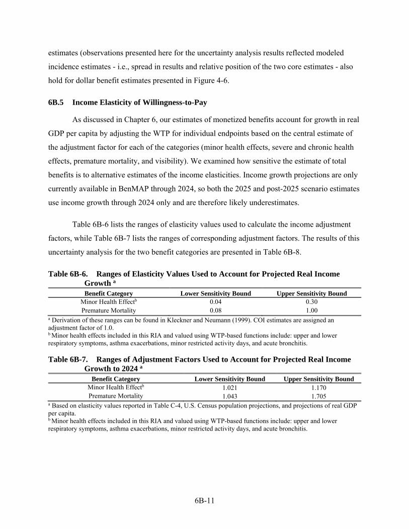
6B-11
estimates (observations presented here for the uncertainty analysis results reflected modeled
incidence estimates - i.e., spread in results and relative position of the two core estimates - also
hold for dollar benefit estimates presented in Figure 4-6.
6B.5 Income Elasticity of Willingness-to-Pay
As discussed in Chapter 6, our estimates of monetized benefits account for growth in real
GDP per capita by adjusting the WTP for individual endpoints based on the central estimate of
the adjustment factor for each of the categories (minor health effects, severe and chronic health
effects, premature mortality, and visibility). We examined how sensitive the estimate of total
benefits is to alternative estimates of the income elasticities. Income growth projections are only
currently available in BenMAP through 2024, so both the 2025 and post-2025 scenario estimates
use income growth through 2024 only and are therefore likely underestimates.
Table 6B-6 lists the ranges of elasticity values used to calculate the income adjustment
factors, while Table 6B-7 lists the ranges of corresponding adjustment factors. The results of this
uncertainty analysis for the two benefit categories are presented in Table 6B-8.
Table 6B-6. Ranges of Elasticity Values Used to Account for Projected Real Income Growth a Benefit Category Lower Sensitivity Bound Upper Sensitivity Bound
Minor Health Effectb 0.04 0.30 Premature Mortality 0.08 1.00
a Derivation of these ranges can be found in Kleckner and Neumann (1999). COI estimates are assigned an adjustment factor of 1.0. b Minor health effects included in this RIA and valued using WTP-based functions include: upper and lower respiratory symptoms, asthma exacerbations, minor restricted activity days, and acute bronchitis.
Table 6B-7. Ranges of Adjustment Factors Used to Account for Projected Real Income
Growth to 2024 a Benefit Category Lower Sensitivity Bound Upper Sensitivity Bound
Minor Health Effectb 1.021 1.170 Premature Mortality 1.043 1.705
a Based on elasticity values reported in Table C-4, U.S. Census population projections, and projections of real GDP per capita. b Minor health effects included in this RIA and valued using WTP-based functions include: upper and lower respiratory symptoms, asthma exacerbations, minor restricted activity days, and acute bronchitis.

6B-12
Table 6B-8. Sensitivity of Monetized Ozone Benefits to Alternative Income Elasticities in 2025 (Millions of 2011$) a
Benefit Category No adjustment Lower Sensitivity Bound Upper Sensitivity Bound
70 ppb 65 ppb 70 ppb 65 ppb 70 ppb 65 ppb Minor Health Effect b $31 $150 $33 $162 $38 $186 Premature Mortality c $950 $4,100 $1,000 $5,200 $1,700 $8,500
a All estimates rounded to two significant digits. Only reflects income growth to 2024. b For illustrative purposes, we evaluate minor restricted activity days (MRADS) resulting from short-term ozone exposure is the minor health effect here. c Short-term mortality using Smith et al. (2009) and 3% discount rate. Results using other short-term mortality studies and a 7% discount rate would show the same proportional range.
Consistent with the impact of mortality on total benefits, the adjustment factor for
mortality has the largest impact on total benefits. The value of mortality in 2025 ranges from 8%
to 76% greater than the core estimate for mortality based on the lower and upper sensitivity
bounds on the mortality income adjustment factor. The effect on the value of minor health effects
is much less pronounced, ranging from 5% to 21% greater than the core estimate for minor
effects. These observations (in terms of relative impact from alternative elasticities) hold for the
revised and alternative standard levels analyzed under both the 2025 and post-205 scenarios.
6B.6 Age Group-Differentiated Aspects of Short-Term Ozone Exposure-Related Mortality
In their 2008 review of the EPA’s approach to estimating ozone-related mortality
benefits, the National Research Council (NRC) indicated, “EPA should consider placing greater
emphasis on reporting decreases in age-specific death rates in the relevant population and
develop models for consistent calculation of changes in life expectancy and changes in number
of deaths at all ages” (NRC, 2008). In addition, NRC noted in an earlier report that “[f]rom a
public-health perspective, life-years lost might be more relevant than annual number of mortality
cases” (NRC, 2002). This advice is consistent with that of the Health Effects Subcommittee of
the Advisory Council on Clean Air Compliance Analysis (SAB-HES), which agreed that “…the
interpretation of mortality risk results is enhanced if estimates of lost life-years can be made”
(U.S. EPA-SAB, 2004). To address these recommendations, we use simplifying assumptions to
estimate the number of life years that might be gained. We also estimate the reduction in the
percentage of deaths attributed to ozone resulting from the illustrative emissions reduction
strategies to reach the revised and alternative primary standards. The EPA included similar
estimates of life years gained in a previous assessment of ozone and/or PM2.5 benefits (U.S. EPA,

6B-13
2006, 2010, 2011a), the latter of which was peer reviewed by the SAB-HES (U.S. EPA-SAB,
2010a).
Changes in life years and changes in life expectancy at birth are frequently conflated,
thus it is important to distinguish these two very different metrics. Life expectancy varies by age.
The Centers for Disease Control and Prevention (CDC) defines life expectancy as the “average
number of years of life remaining for persons who have attained a given age” (CDC, 2011). In
other words, changes in life expectancy refer to an average change for the entire population, and
refer to the future. Over the past 50 years, average life expectancy at birth in the U.S. has
increased by 8.4 years (CDC, 2011). For example, life expectancy at birth was estimated in 2007
to be 77.9 years for an average person born in the U.S., but for people surviving to age 60,
estimated life expectancy is 82.5 years (i.e., 4.6 years more than life expectancy at birth) (CDC,
2011). Life years, on the other hand, measure the amount of time that an individual loses if they
die before the age of their life expectancy. Life years refer to individuals, and refer to the past,
e.g., when the individual has already died. If a 60-year old individual dies, we estimate that this
individual would lose about 22.5 years of life (i.e., the average population life expectancy for an
individual of this age minus this person’s age at death).
Due to the use of benefit-per-ton estimates for the PM2.5 co-benefits, we are unable to
estimate the life years gained by reducing exposure to PM2.5 in this analysis. Instead, we refer the
reader to the 2012 PM2.5 NAAQs RIA for more information about the avoided life years lost
from PM2.5 exposure (U.S. EPA, 2012b). The analysis performed for the PM NAAQS RIA found
that about half of the avoided PM-related deaths occur in populations age 75 to 99, but half of
the avoided life years lost would occur in populations younger than 65 because the younger
populations have the potential to lose more life years per death than older populations. In
addition, that analysis found that the average individual who would otherwise have died
prematurely from PM exposure would gain 16 additional years of life.
Estimated Life Years Gained
To estimate the potential life years gained by reducing exposure to ozone in the U.S.
adult population, we use the same general approach as Hubbell (2006) and Fann et al. (2012).
We have not estimated the change in average life expectancy at birth in this RIA. Because life

6B-14
expectancy is an average of the entire population (including both those whose deaths would
likely be attributed to air pollution exposure as well as those whose deaths would not), we would
expect average life expectancy changes associated with air pollution exposure to always be
significantly smaller than the average number of life years lost by an individual projected to die
prematurely from air pollution exposure.
To estimate the potential distribution of life years gained for population subgroups
defined by the age range at which their reduction in air pollution exposure is modeled to occur,
we use standard life tables available from the CDC (2014) and the following formula:
∑ (6.2)
where LEi is the average remaining life expectancy for age interval i, Mi is the estimated change
in number of deaths in age interval i, and n is the number of age intervals.
To get Mi (the estimated number of avoided premature deaths attributed to changes in
ozone exposure for the 2025 scenario), we use a health impact function that incorporates risk
coefficients estimated for the adult population in the U.S. and age-specific mortality rates. That
is, we use risk coefficients that do not vary by age, but use baseline mortality rates that do.
Because mortality rates for younger populations are much lower than mortality rates for older
populations, most but not all, of the avoided deaths tend to be in older populations. Table 6B-9
summarizes the number of avoided deaths (by age range) attributable to ozone for the revised
and alternative standards for the 2025 scenario. Table 6B-10 summarizes the modeled number of
life years gained (for each age range) by reducing ozone for the revised and alternative standards
analyzed for the 2025 scenario. We then calculated the average number of life years gained per
avoided premature mortality.

6B-15
Table 6B-9. Potential Reduction in Premature Mortality by Age Range from Attaining the Revised and Alternative Ozone Standards (2025 scenario) a, b
Age Range b
Revised and Alternative Standards 70 ppb 65 ppb
0-4 0.3 1.5 5-9 0.068 0.33
10-14 0.072 0.35 15-19 0.1 0.5 20-24 0.14 0.69 25–29 0.29 1.4 30–34 0.3 1.5 35–44 1.6 7.9 45–54 4.1 20 55–64 10 52 65–74 22 110 75–84 29 150 85–99 28 150
Total ozone-attributable mortality 96 490 a Estimates rounded to two significant digits. b Effects calculated using Smith et al. (2009). Table 6B-10. Potential Years of Life Gained by Age Range from Attaining the Revised and
Alternative Ozone Standards (2025 Scenario) a,b Age Range b
Revised and Alternative Standard
70 ppb 65 ppb 0-4 24 110 5-9 5 23
10-14 5 23 15-19 6 30 20-24 8 38 25–29 14 70 30–34 13 66 35–44 57 280 45–54 110 550 55–64 200 990 65–74 260 1,300 75–84 190 970 85–99 65 340
Total life years gained 960 4,800 Average life years gained per individual 10 10
a Estimates rounded to two significant digits. b Effects calculated using Smith et al. (2009).
By comparing the projected age distribution of the avoided premature deaths with the age
distribution of life years gained, we observed that about half of the deaths occur in populations
age 75–99 (see Table 6B-9), but half of the life years would occur in populations younger than

6B-16
65 (see Table 6B-10). This is because the younger populations have the potential to lose more
life years per death than older populations based on changes in ozone exposure for the 2025
scenario. We estimate that the average individual who would otherwise have died prematurely
from ozone exposure would gain 10 additional years of life. However, this approach does not
account for whether or not people who are older are more likely to be susceptible to the health
effects of air pollution or whether that susceptibility was caused by air pollution exposure (for a
more complete discussion of this issue, see Kunzli et al., 2001).
Percent of Ozone-related Mortality Reduced
To estimate the percentage reduction in all-cause mortality attributed to reduced ozone
exposure for the 2025 scenario as a result of the illustrative emissions reduction strategies, we
use Mi from the equation above, dividing the number of excess deaths estimated for the revised
and alternative standards by the total number of deaths in each county. Table 6B-11 shows the
reduction in all-cause mortality attributed to reducing ozone exposure to the revised and
alternative primary standards for the 2025 scenario.
Table 6B-11. Estimated Percent Reduction in All-Cause Mortality Attributed to the Proposed Primary Ozone Standards (2025 Scenario) a
Age Range b
Revised and Alternative Standards 70 ppb 65 ppb
0-4 0.0085% 0.0409% 5-9 0.0084% 0.0411%
10-14 0.0084% 0.0415% 15-19 0.0086% 0.0419% 20-24 0.0085% 0.0412% 25–29 0.0084% 0.0409% 30–34 0.0083% 0.0408% 35–44 0.0081% 0.0404% 45–54 0.0082% 0.0410% 55–64 0.0085% 0.0429% 65–74 0.0086% 0.0436% 75–84 0.0085% 0.0433% 85–99 0.0079% 0.0415%
a To illustrate the slight variations in percent reductions across age ranges, we present results rounded to three significant digits (rather than two as is typically done for other estimates in this RIA).
Results presented in Table 6B-11 highlight that when reductions in ozone-attributable
mortality (in going from baseline to the revised or alternative standard level) are considered as a
6B-17
percentage of total all-cause baseline mortality, the estimates are relatively small and are fairly
constant across age ranges. However, it is important to point out that estimates of total ozone-
attributable mortality represent a substantially larger fraction of all-cause baseline mortality.
6B.7 Evaluation of Mortality Impacts Relative to the Baseline Pollutant Concentrations for both Short-Term Ozone Exposure-Related Mortality and Long-Term PM2.5 Exposure-Related Mortality
Analysis of baseline ozone levels used in modeling short-term ozone exposure-related mortality
Our review of the current body of scientific literature indicates that a log-linear no-
threshold model provides the best estimate of ozone-related short-term mortality (see section
2.5.4.4, in the O3 ISA, U.S. EPA, 2013). Consistent with this finding, we estimate benefits
associated with the full range of ozone exposure. Our confidence in the estimated number of
premature deaths avoided (but not in the existence of a causal relationship between ozone and
premature mortality) diminishes as we estimate these impacts at successively lower
concentrations. However, there are uncertainties inherent in identifying any particular point at
which our confidence in reported associations becomes appreciably less, and the scientific
evidence provides no clear dividing line. The O3 ISA noted that the studies indicate reduced
certainty in specifying the shape of the C-R function specifically for short-term ozone-
attributable respiratory morbidity and mortality, in the range generally below 20 ppb (for these
reasons, the ≤ 20 ppb range discussed in the O3 ISA should be viewed as a more generalized
range to be considered qualitatively or semi-quantitatively, along with many other factors, when
interpreting the risk estimates rather than as a fixed, bright-line).
Figures 6B-1 and 6B-2 compare the distribution of short-term ozone exposure-related
mortality to the underlying distribution of the summer season 8-hour maximum ozone
concentrations. Both figures (probability and cumulative probability) are based on Smith et al.
(2009) using mortality results at each 12 km grid cell and the associated summer season 8-hour
maximum concentration in the baseline. In addition, each figure includes separate plots for the
revised and alternative standard levels. Figure 6B-1 shows that approximately 45% of the
premature mortalities estimated for the 65 ppb alternative standard is associated with baseline
ozone concentrations between 40 and 45 ppb. Because this baseline range is represents the mean

6B-18
across the ozone season of 8-hour max values within a given grid cell, the actual distribution of
8-hour max values on a daily basis is likely wider than the 40-45 ppb range.
Figure 6B-1. Premature Ozone-related Deaths Avoided for the Revised and Alternative Standards (2025 scenario) According to the Baseline Ozone Concentrations
0%
5%
10%
15%
20%
25%
30%
35%
40%
45%
50%
0 to 15
15 to 20
20 to 25
25 to 30
30 to 35
35 to 40
40 to 45
45 to 50
50 to 55
55 to 60
60 to 65
65 to 70
70 to 75
75 to 80
Percentage of reductionin short‐term ozone
related m
ortality
Ozone season mean daily 8hr max baseline (ppb)
75‐70 75‐65

6B-19
Figure 6B-2. Cumulative Probability Plot of Premature Ozone-related Deaths Avoided for the Revised and Alternative Standards (2025 scenario) According to the Baseline Ozone Concentrations
When interpreting these results, it is important to understand that the avoided ozone-
related deaths are estimated to occur from ozone reductions in the baseline air quality simulation,
which assumes that 75 ppb is already met. When simulating attainment with the revised and
alternative standards, we adjust the design value at each monitor exceeding the standard to equal
that standard and use an air quality interpolation technique to simulate the change in ozone
concentrations surrounding that monitor. This technique tends to simulate the greatest air quality
changes nearest the monitor. We estimate benefits using modeled air quality data with 12 km
grid cells, which is important because the grid cells are often substantially smaller than counties
and ozone concentrations vary spatially within a county. Therefore, there may be a small number
of grid cells with concentrations slightly greater than 75 ppb in the gridded baseline even though
all monitors could meet an annual standard of 75 ppb. In addition, some grid cells in a county
can be below the level of a standard even though the highest monitor value is above that
standard. Thus, emissions reductions can lead to benefits in grid cells that are below a standard
even within a county with a monitor that exceeds that standard. Furthermore, our approach to
0
0.2
0.4
0.6
0.8
1
1.2
0 to 15
15 to 20
20 to 25
25 to 30
30 to 35
35 to 40
40 to 45
45 to 50
50 to 55
55 to 60
60 to 65
65 to 70
70 to 75
75 to 80
Cumulative percentage of reductionin
short‐term ozone related m
ortality
Ozone season mean daily 8hr max baseline (ppb)
75‐70 75‐65

6B-20
simulating attainment can lead to benefits in counties that are below the revised or alternative
standard being evaluated. Emissions reduction strategies designed to reduce ozone
concentrations at a given monitor will frequently improve air quality in neighboring counties. In
order to make a direct comparison between the benefits and costs of these emissions reduction
strategies, it is appropriate to include all the benefits occurring as a result of the emissions
reduction strategies applied, regardless of where they occur. Therefore, it is not appropriate to
estimate the fraction of benefits that occur only in counties that exceed the revised or alternative
standards because it would omit benefits attributable to emissions reductions in non-exceeding
counties.
One final caveat in interpreting the information presented in these figures is that in
modeling this mortality endpoint, rather than using a true distribution of daily 8hr max ozone
levels for each grid cell, due to resource limitations, we used a single mean value for the ozone
season within each grid cell. While this will generate the same total ozone benefit estimate for
each grid cell compared with application of a full distribution of daily 8hr max values, use of a
mean daily value means that an assessment such as this one, that considers both the spatial and
temporal association between mortality benefit estimates and ozone levels, will be limited
somewhat in its treatment of the temporal dimension.
As shown in Figures 6B-1 and 6B-2, the vast majority of reductions in short-term
exposure-related mortality for ozone occur in grid cells with mean 8-hour max baseline levels
(across the ozone season) between 35 and 55 ppb. Comparing patterns across the revised and
alternative standard levels, the upper end of the distribution shifts downwards as increasingly
lower standard levels are analyzed (see Figure 6B-2).
Concentration Benchmark Analysis for PM2.5 Benefit-per-ton Estimates
In general, we are more confident in the magnitude of the risks we estimate from simulated
PM2.5 concentrations that coincide with the bulk of the observed PM concentrations in the
epidemiological studies that are used to estimate the benefits. Likewise, we are less confident in
the risk we estimate from simulated PM2.5 concentrations that fall below the bulk of the observed
data in these studies. Concentration benchmark analyses (e.g., lowest measured level [LML], one
standard deviation below the mean of the air quality data in the study, etc.) allow readers to

6B-21
determine the portion of population exposed to annual mean PM2.5 levels at or above different
concentrations, which provides some insight into the level of uncertainty in the estimated PM2.5
mortality benefits. In this analysis, we apply two concentration benchmark approaches (LML and
one standard deviation below the mean) that have been incorporated into recent RIAs and EPA’s
Policy Assessment for Particulate Matter (U.S. EPA, 2011c). There are uncertainties inherent in
identifying any particular point at which our confidence in reported associations becomes
appreciably less, and the scientific evidence provides no clear dividing line. However, the EPA
does not view these concentration benchmarks as a concentration threshold below which we
would not quantify health co-benefits of air quality improvements.173 Rather, the co-benefits
estimates reported in this RIA are the best estimates because they reflect the full range of air
quality concentrations associated with the emissions reduction strategies. The PM ISA concluded
that the scientific evidence collectively is sufficient to conclude that the relationship between
long-term PM2.5 exposures and mortality is causal and that overall the studies support the use of a
no-threshold log-linear model to estimate PM-related long-term mortality (U.S. EPA, 2009).
For this analysis, policy-specific air quality data is not available, and the compliance
strategies are illustrative of what states may choose to do. For this RIA, we are unable to
estimate the percentage of premature mortality associated with the emissions reductions at each
PM2.5 concentration, as we have done for previous rules with air quality modeling (e.g., U.S.
EPA, 2011b, 2012b). However, we believe that it is still important to characterize the distribution
of exposure to baseline concentrations. As a surrogate measure of mortality impacts, we provide
the percentage of the population exposed at each PM2.5 concentration in the baseline of the
source apportionment modeling used to calculate the benefit-per-ton estimates for this sector
using 12 km grid cells across the contiguous U.S.174 It is important to note that baseline exposure
is only one parameter in the health impact function, along with baseline incidence rates,
population and change in air quality. In other words, the percentage of the population exposed to
173 For a summary of the scientific review statements regarding the lack of a threshold in the PM2.5-mortality
relationship, see the TSD entitled Summary of Expert Opinions on the Existence of a Threshold in the Concentration-Response Function for PM2.5-related Mortality (U.S. EPA, 2010b).
174 As noted above, the modeling used to generate the benefit-per-ton estimates does not reflect emissions reductions anticipated from MATS rule. Therefore, the baseline PM2.5 concentrations in the LML assessment are higher than would be expected if MATS was reflected.

6B-22
air pollution below the LML is not the same as the percentage of the population experiencing
health impacts as a result of a specific emissions reduction policy. The most important aspect,
which we are unable to quantify without rule-specific air quality modeling, is the shift in
exposure anticipated by the revised or alternative standards. Therefore, caution is warranted
when interpreting the LML assessment in this RIA because these results are not consistent with
results from RIAs that had air quality modeling.
Table 6B-12 provides the percentage of the population exposed above and below two
concentration benchmarks in the modeled baseline for the sector modeling. Figure 6B-3 shows a
bar chart of the percentage of the population exposed to various air quality levels in the baseline,
and Figure 6B-4 shows a cumulative distribution function of the same data. Both figures identify
the LML for each of the major cohort studies.

6B-23
Table 6B-12. Population Exposure in the Baseline Sector Modeling (used to generate the benefit-per-ton estimates) Above and Below Various Concentration Benchmarks in the Underlying Epidemiology Studies a
Epidemiology Study Below 1 Standard
Deviation. Below AQ Mean
At or Above 1 Standard Deviation Below AQ Mean
Below LML At or Above LML
Krewski et al. (2009) 89% 11% 7% 93% Lepeule et al. (2012) N/A N/A 23% 67%
a One standard deviation below the mean is equivalent to the middle of the range between the 10th and 25th percentile. For Krewski et al., the LML is 5.8 µg/m3 and one standard deviation below the mean is 11.0 µg/m3. For Lepeule et al., the LML is 8 µg/m3 and we do not have the data for one standard deviation below the mean. It is important to emphasize that although we have lower levels of confidence in levels below the LML for each study, the scientific evidence does not support the existence of a level below which health effects from exposure to PM2.5 do not occur.
Figure 6B-3. Percentage of Adult Population (age 30+) by Annual Mean PM2.5 Exposure in
the Baseline Sector Modeling (used to generate the benefit-per-ton estimates)*
* This graph shows the population exposure in the modeling baseline used to generate the benefit-per-ton estimates. Similar graphs for analyses with air quality modeling show premature mortality impacts at each PM2.5 concentration. Therefore, caution is warranted when interpreting this graph because it is not consistent with similar graphs from RIAs that had air quality modeling (e.g., MATS).
Among the populations exposed to PM2.5 in the baseline: 93% are exposed to PM2.5 levels at or above the LML of the Krewski et al. (2009) study 67% are exposed to PM2.5 levels at or above the LML of the Lepeule et al. (2012) study
0%
5%
10%
15%
20%
25%
<1 1‐2 2‐3 3‐4 4‐5 5‐6 6‐7 7‐8 8‐9 9‐10 10‐11 11‐12 12‐13 13‐14 14‐15 15‐16 16‐17 17‐18 18‐19 19‐20
Percentage
of Population Exposed
Baseline Annual Mean PM2.5 Level (µg/m3)
LML of Lepeule et al. (2012) study
LML of Krewski et al. (2009) study

6B-24
Figure 6B-4. Cumulative Distribution of Adult Population (age 30+) by Annual Mean
PM2.5 Exposure in the Baseline Sector Modeling (used to generate the benefit-per-ton estimates)*
* This graph shows the population exposure in the modeling baseline used to generate the benefit-per-ton estimates. Similar graphs for analyses with air quality modeling show premature mortality impacts at each PM2.5 concentration. Therefore, caution is warranted when interpreting this graph because it is not consistent with similar graphs from RIAs that had air quality modeling (e.g., MATS).
6B.8 Ozone-related Impacts on Outdoor Worker Productivity
The EPA last quantified the value of ozone-related worker productivity in the final
Regulatory Impact Analysis supporting the Transport Rule (U.S. EPA, 2011d). That analysis
applied information reported in Crocker and Horst (1981) to relate changes in ground-level
ozone to changes in the productivity of outdoor citrus workers. That study found that a 10
percent reduction in ozone translated to a 1.4 increase in income among outdoor citrus workers.
Concerned that this study might not adequately characterize the relationship between ground-
Among the populations exposed to PM2.5 in the baseline: 93% are exposed to PM2.5 levels at or above the LML of the Krewski et al. (2009) study 67% are exposed to PM2.5 levels at or above the LML of the Lepeule et al. (2012) study
0%
10%
20%
30%
40%
50%
60%
70%
80%
90%
100%
1 2 3 4 5 6 7 8 9 10 11 12 13 14 15 16 17 18 19 20
Cumulative
percentage
of population exposed
Baseline Annual Mean PM2 5Level (µg/m3)
LML of Krewski et al. (2009) study
LML of Lepeule et al. (2012) study

6B-25
level ozone and the productivity of agricultural workers because of the vintage of the underlying
data, the Agency subsequently omitted this endpoint.
In a recent study, Graff Zivin and Neidell (2012) combined data on individual-level daily
harvest rates for Outdoor Agricultural Workers (OWAs) with ground-level ozone concentrations
to characterize changes in worker productivity as a result of ozone exposure. The authors used
data on harvest rates from a 500-acre farm in the Central Valley of California. That farm
produced three crops (blueberries and two types of grapes) and the harvesting laborers were paid
through piece rate contracts. The analyses in the paper were based on 2009 and 2010 California
growing seasons. The analyses were not affected by: (i) endogenous ozone exposure (because
there were limited local sources of ozone precursors); (ii) avoidance behavior (because the work
has to be performed outdoors); and (iii) shirking (due to the nature of the piece rate contract).
Table 3 in Graff Zivin and Neidell (2012) reports the main result: A 10 ppb increase in
work-day ozone concentration (represented by hourly measurements averaged between 6am and
3pm) will result in a decline of 0.143 (with a standard error of 0.068) in standardized hourly
pieces collected on a given work day. The standardized hourly pieces were “the average hourly
productivity minus the minimum number of pieces per hour required to reach the piece rate
regime, divided by the standard deviation of productivity for each crop” (Graff Zivin and
Neidell, 2012; p. 3665). The range of ozone concentrations in the sample was between 10.50 ppb
and 86.0 ppb (Table 1 in Graff Zivin and Neidell, 2012). This result is significant and robust
under different model specifications designed to test modeling assumptions. Based on the effect
estimate and individual-level information in their dataset, the authors estimated the effect of an
increase in ozone concentration on worker productivity, as measured by the average number of
pieces collected per hour during a given work day (rather than by standardized hourly piece rate
that was used in regression modeling). They found a decline of 5.5% in worker productivity due
to a 10 ppb increase in average work-day ozone concentration.
While Graff Zivin and Neidell (2012) report the information needed to quantify ozone-
related worker productivity, we are still evaluating whether and how to most appropriately apply
the limited evidence from this study in a national benefits assessment. An important issue is the
generalizability of the results to the appropriate population. We recognize that there is

6B-26
significant uncertainty in the generalizability of this study and the need for additional research
and peer review in guiding the monetization of agriculatural productivity impacts. Because we
received no comments on this proposed approach, we now include the results as part of our
uncertainty analysis.
Below we provide the function, input data and results for the analysis.
∗ ∗ ∗ ∗ Table 6B-13. Definitions of Variables Used to Calculate Changes in Worker Productivity
Variable Definition
Percent change in daily outdoor worker productivity per 1ppb change in ozone (Graff Zivin and Neidell, 2012)
Summer season average of daily 9 hour average (6am to 3pm)
Summer season daily wage for agricultural non-livestock workers in 17 USDA-defined regions (USDA, 2012)
Summer season number of workers employed in outdoor non-livestock agricultural per county (USDA, 2010; US Census, 2010)
Growth in agricultural non-livestock workers to 2025 (Woods and Poole, 2012)
Table 6B-14. Population Estimated Economic Value of Increased Productivity among
Outdoor Agricultural Workers from Attaining the Revised and Alternative Ozone Standards in 2025 (millions of 2011$)
Standard Economic Value
(95th percentile confidence interval)
70 ppb $1.7
($0.1 to $3.3)
65 ppb $8.9
($0.6 to $17)
6B.9 References
Centers for Disease Control and Prevention (CDC). 2011. United States Life Tables, 2007 National Vital Statistics Reports. Volume 59, Number 9. September. Available at <http://www.cdc.gov/nchs/data/nvsr/nvsr59/nvsr59_09.pdf>.
Centers for Disease Control and Prevention (CDC). 2014. Health, United States. Table 19. Years of Potential Life Lost Before Age 75 for Selected Causes of Death, According to Sex, Race and Hispanic Origin: United States, Selected Years 1980–2013 (2014).
Crocker, T. D., & Horst, R. L. 1981. “Hours of work, labor productivity, and environmental conditions: A case study.” The Review of Economics and Statistics 63(3), 361-368.
Crouse, DL; Peters, PA; van Donkelaar, A; Goldberg, MS; Villeneuve, PJ; Brion, O; Khan, S; Atari, DO; Jerrett, M; Pope, CA; Brauer, M; Brook, JR; Martin, RV; Stieb, D; Burnett, RT. 2012.” Risk of nonaccidental and

6B-27
cardiovascular mortality in relation to long-term exposure to low concentrations of fine particulate matter: a Canadian national-level cohort study.” Environ Health Perspect 120: 708-714.
Eftim SE, Samet JM, Janes H, McDermott A, Dominici F. 2008. “Fine Particulate Matter and Mortality: A Comparison of the Six Cities and American Cancer Society Cohorts with a Medicare Cohort.” Epidemiology 19: 209- 216.
Fann N, Lamson A, Wesson K, Risley D, Anenberg SC, Hubbell BJ. 2012. “Estimating the National Public Health Burden Associated with Exposure to Ambient PM2.5 and ozone. Risk Analysis,” Risk Analysis 32(1): 81-95.
Graff Zivin, J., Neidell, M. (2012). The impact of pollution on worker productivity. American Economic Review 102, 3652-3673.
Hubbell BL. 2006. “Implementing QALYs in the analysis of air pollution regulations.” Environmental and Resource Economics 34:365–384.
Industrial Economics, Incorporated (IEc). 2006. Expanded Expert Judgment Assessment of the Concentration-Response Relationship Between PM2.5 Exposure and Mortality. Prepared for: Office of Air Quality Planning and Standards, U.S. Environmental Protection Agency, Research Triangle Park, NC. September. Available at <http://www.epa.gov/ttn/ecas/regdata/Uncertainty/pm_ee_tsd_expert_interview_summaries.pdf>.
Jerrett M, Burnett RT, Pope CA, III, et al. 2009. “Long-Term Ozone Exposure and Mortality.” New England Journal of Medicine 360:1085-95.
Kleckner, N., and J. Neumann. 1999. “Recommended Approach to Adjusting WTP Estimates to Reflect Changes in Real Income.” Memorandum to Jim DeMocker, US EPA/OPAR. June 3, Available on the Internet at <http://www.epa.gov/ttn/ecas/regdata/Benefits/background/klecknerandneumann1999.pdf>.
Krewski D, Jerrett M, Burnett RT, Ma R, Hughes E, Shi, Y, et al. 2009. Extended follow-up and spatial analysis of the American Cancer Society study linking particulate air pollution and mortality. HEI Research Report, 140, Health Effects Institute, Boston, MA.
Kunzli, N., S. Medina, R. Kaiser, P. Quenel, F. Horak Jr, and M. Studnicka. 2001. “Assessment of Deaths Attributable to Air Pollution: Should We Use Risk Estimates Based on Time Series or on Cohort Studies?” American Journal of Epidemiology 153(11):1050-55.
Laden F; Schwartz J; Speizer FE; Dockery DW. 2006. “Reduction in fine particulate air pollution and mortality: extended follow-up of the Harvard Six Cities study.” Am J Respir Crit Care Med, 173: 667-672.
Lepeule J, Laden F, Dockery D, Schwartz J. 2012. “Chronic Exposure to Fine Particles and Mortality: An Extended Follow-Up of the Harvard Six Cities Study from 1974 to 2009.” Environmental Health Perspectives 120 (7):965-70.
Lipfert FW; Baty JD; Miller JP; Wyzga RE (2006). “PM2.5 constituents and related air quality variables as predictors of survival in a cohort of U.S. military veterans.” Inhal Toxicol, 18: 645-657.
Mansfield and Patil, 2006. Peer Review of Expert Elicitation. Memo from RTI International to Ron Evans, EPA. September 26. Available at <http://www.epa.gov/ttn/ecas/regdata/Uncertainty/peer_review_summary_rti_29sept06.pdf>.
Miller KA, Siscovick DS, Sheppard L, Shepherd K, Sullivan JH, Anderson GL, Kaufman JD. (2007). “Long-term exposure to air pollution and incidence of cardiovascular events in women” N Engl J Med, 356: 447-458.
National Research Council (NRC). 2002. Estimating the Public Health Benefits of Proposed Air Pollution Regulations. Washington, DC: The National Academies Press. Washington, DC.

6B-28
National Research Council (NRC). 2008. Estimating Mortality Risk Reduction and Economic Benefits from Controlling Ozone Air Pollution. National Academies Press. Washington, DC.
Pope, C.A. III; Burnett, R.T.; Thun, M.J.; Calle, E.E.; Krewski, D.; Ito, K.; Thurston G.D. 2002. “Lung cancer, cardiopulmonary mortality, and long-term exposure to fine particulate air pollution.” JAMA 287(9):1132-1141.
Puett, RC; Hart, JE; Suh, H; Mittleman, M; Laden, F. (2011). “Particulate matter exposures, mortality and cardiovascular disease in the health professionals follow-up study.” Environ Health Perspect 119: 1130-1135. http://dx.doi.org/10.1289/ehp.1002921
Puett, RC; Hart, JE; Yanosky, JD; Paciorek, C; Schwartz, J; Suh, H; Speizer, FE; Laden, F. 2009. “Chronic fine and coarse particulate exposure, mortality, and coronary heart disease in the Nurses' Health Study.” Environ Health Perspect 117: 1697-1701. http://dx.doi.org/10.1289/ehp.0900572
Roman, Henry A., Katherine D. Walker, Tyra L. Walsh, Lisa Conner, Harvey M. Richmond, Bryan J. Hubbell, and Patrick L. Kinney. 2008. “Expert Judgment Assessment of the Mortality Impact of Changes in Ambient Fine Particulate Matter in the U.S.” Environmental Science & Technology 42(7):2268-2274.
Sasser, E. 2014. Response to Comments Regarding the Potential Use of a Threshold Model in Estimating the Mortality Risks from Long-term Exposure to Ozone in the Health Risk and Exposure Assessment for Ozone, Second External Review Draft. Memorandum to Holly Stallworth, Designated Federal Officer, Clean Air Scientific Advisory Committee from EPA/OAQPS Health and Environmental Impacts Division.
Smith, R.L.; B. Xu and P. Switzer. 2009. Reassessing the relationship between ozone and short- term mortality in U.S. urban communities. Inhalation Toxicology 21:37-61.
U.S. Environmental Protection Agency (U.S. EPA). 2006. Final Regulatory Impact Analysis (RIA) for the PM2.5 National Ambient Air Quality Standards (NAAQS). Office of Air Quality Planning and Standards, Research Triangle Park, NC. Available at < http://www.epa.gov/ttn/ecas/regdata/RIAs/Chapter%205--Benefits.pdf >.
U.S. Environmental Protection Agency (U.S. EPA). 2009. Integrated Science Assessment for Particulate Matter: Final. U.S. Environmental Protection Agency, Research Triangle Park, NC, EPA/600/R-08/139F. Available at <http://cfpub.epa.gov/ncea/cfm/recordisplay.cfm?deid=216546>.
U.S. Environmental Protection Agency (U.S. EPA). 2010. Final Regulatory Impact Analysis (RIA) for the SO2 National Ambient Air Quality Standards (NAAQS). Office of Air Quality Planning and Standards, Research Triangle Park, NC. June. Available at <http://www.epa.gov/ttn/ecas/regdata/RIAs/fso2ria100602full.pdf>.
U.S. Environmental Protection Agency (U.S. EPA). 2011a. The Benefits and Costs of the Clean Air Act 1990 to 2020: EPA Report to Congress. Office of Air and Radiation, Office of Policy, Washington, DC. March. Available at <http://www.epa.gov/oar/sect812/feb11/fullreport.pdf>.
U.S. Environmental Protection Agency (U.S. EPA). 2011b. Regulatory Impact Analysis for the Final Mercury and Air Toxics Standards. EPA-452/R-11-011. December. Available at: <http://www.epa.gov/ttn/ecas/regdata/RIAs/matsriafinal.pdf>.
U.S. Environmental Protection Agency (U.S. EPA). 2011c. Policy Assessment for the Review of the Particulate Matter National Ambient Air Quality Standards. EPA-452/D-11-003. April. Available on the Internet at <http://www.epa.gov/ttnnaaqs/standards/pm/s_pm_2007_pa.html>.
U.S. Environmental Protection Agency (U.S. EPA). 2011d. Regulatory Impact Analysis for the Federal Implementation Plans to Reduce Interstate Transport of Fine Particulate Matter and ozone in 27 States; Correction of SIP Approvals for 22 States. June. Available at <http://www.epa.gov/airtransport/pdfs/FinalRIA.pdf>.

6B-29
U.S. Environmental Protection Agency (U.S. EPA). 2012a. Provisional Assessment of Recent Studies on Health Effects of Particulate Matter Exposure. Office of Research and Development, Research Triangle Park, NC. December 2012, EPA/600/R-12/056F. Available at <http://www.epa.gov/ttn/naaqs/standards/pm/data/20121213psa.pdf >.
U.S. Environmental Protection Agency (U.S. EPA). 2012b. Regulatory Impact Analysis for the Final Revisions to the National Ambient Air Quality Standards for Particulate Matter. EPA-452/R-12-003. Office of Air Quality Planning and Standards, Health and Environmental Impacts Division. December. Available at: <http://www.epa.gov/pm/2012/finalria.pdf>.
U.S. Environmental Protection Agency (U.S. EPA). 2013. Integrated Science Assessment for Ozone and Related Photochemical Oxidants: Final. Research Triangle Park, NC: U.S. Environmental Protection Agency. (EPA document number EPA/600/R-10/076F).
U.S. Environmental Protection Agency Science Advisory Board (U.S. EPA-SAB). 2004. Advisory on Plans for Health Effects Analysis in the Analytical Plan for EPA’s Second Prospective Analysis—Benefits and Costs of the Clean Air Act, 1990-2020: Advisory by the Health Effects Subcommittee of the Advisory Council on Clean Air Compliance Analysis. EPA-SAB-COUNCIL-ADV-04-002. March. Available on the Internet at <http://yosemite.epa.gov/sab%5CSABPRODUCT.NSF/08E1155AD24F871C85256E5400433D5D/$File/council_adv_04002.pdf>.
U.S. Environmental Protection Agency Science Advisory Board (U.S. EPA-SAB). 2008. Characterizing Uncertainty in Particulate Matter Benefits Using Expert Elicitation. EPA-COUNCIL-08-002. July. Available at <http://yosemite.epa.gov/sab/sabproduct.nsf/0/43B91173651AED9E85257487004EA6CB/$File/EPA-COUNCIL-08-002-unsigned.pdf>.
U.S. Environmental Protection Agency Science Advisory Board (U.S. EPA-SAB). 2010. Review of EPA’s DRAFT Health Benefits of the Second Section 812 Prospective Study of the Clean Air Act. EPA-COUNCIL-10-001. June. Available on the Internet at <http://yosemite.epa.gov/sab/sabproduct.nsf/9288428b8eeea4c885257242006935a3/59e06b6c5ca66597852575e7006c5d09!OpenDocument&TableRow=2.3#2.>.
U.S. Environmental Protection Agency Science Advisory Board (U.S. EPA-SAB). 2014. CASAC Review of the EPA’s Health Risk and Exposure Assessment for Ozone (Second External Review Draft – February, 2014). U.S. Environmental Protection Agency Science Advisory Board. EPA-CASAC-14-005. <http://yosemite.epa.gov/sab/sabproduct.nsf/db6b9452a00aa3bd85257242006901de/5F6FB6DEE3442C9485257D08004C707A/$File/EPA-CASAC-14-005+unsigned.pdf>.
Zeger S; Dominici F; McDermott A; Samet J (2008). Mortality in the Medicare population and chronic exposure to fine particulate air pollution in urban centers (2000-2005). Environ Health Perspect, 116: 1614-1619.

7-1
CHAPTER 7: IMPACTS ON PUBLIC WELFARE OF ATTAINMENT STRATEGIES TO MEET PRIMARY AND SECONDARY OZONE NAAQS
Overview
This chapter provides a discussion of the welfare-related benefits of meeting alternative
primary and secondary ozone standards. Welfare benefits of reductions in ambient ozone
include increased growth and/or biomass production in sensitive plant species, including forest
trees, increased crop yields, reductions in visible foliar injury, increased plant vigor (e.g.
decreased susceptibility to harsh weather, disease, insect pest infestation, and competition), and
changes in ecosystems and associated ecosystem services. Although we have not conducted an
analysis to represent the ozone improvements from emissions reductions estimated in the final
RIA, we reference the analysis conducted in the proposal RIA (U.S. EPA, 2014b) as an
indication of the potential magnitude of effects associated with changes in yields of commercial
forests and agriculture, and carbon sequestration and storage. We did not update the analysis
from the proposal RIA because the welfare co-benefits estimates (i) in the proposal analysis were
small, and we anticipated that the estimates in the final analysis would be even smaller, and (ii)
are not added to the human health benefits estimates.
The EPA has also concluded that the current secondary standard for ozone, set at a level of
75 ppb, is not requisite to protect public welfare from known or anticipated adverse effects, and
is revising the standard to provide increased protection against vegetation-related effects on
public welfare. Specifically, the EPA is retaining the indicator (ozone), averaging time (8-hour)
and form (annual fourth-highest daily maximum, averaged over 3 years) of the existing
secondary standard and is revising the level of that standard to 70 ppb. The EPA has concluded
that this revision will effectively curtail cumulative seasonal ozone exposures above 17 ppm-hrs,
in terms of a three-year average seasonal W126 index value, based on the three consecutive
month period within the growing season with the maximum index value, with daily exposures
cumulated for the 12-hour period from 8:00 am to 8:00 pm. Thus, the EPA has concluded that
this revision will provide the requisite protection against known or anticipated adverse effects to
the public welfare.
In addition to the direct welfare benefits of decreased levels of ambient ozone, the
emissions reduction strategies used to demonstrate attainment with alternative ozone standards

7-2
may result in additional benefits associated with reductions in nitrogen deposition and reductions
in ambient concentrations of PM2.5 and its components. These additional benefits include
reductions in nutrient enrichment and acidification impacts on sensitive aquatic and terrestrial
ecosystems and improvements in visibility in state and national parks, wilderness areas, and in
the areas where people live and work. However, we are not able to quantify or monetize these
benefits in this RIA.
7.1 Welfare Benefits of Strategies to Attain Primary and Secondary Ozone Standards
The Clean Air Act defines welfare effects to include any non-health effects, including
direct economic damages in the form of lost productivity of crops and trees, indirect damages
through alteration of ecosystem functions, indirect economic damages through the loss in value
of recreational experiences or the existence value of important resources, and direct damages to
property, either through impacts on material structures or by soiling of surfaces (Section 302(h)
(42 U.S.C. § 7602(h)). For welfare effects associated with changes to ecosystem functions, we
use the concept of ecosystem services as a useful framework for analyzing the impact of
ecosystem changes on public welfare. Ecosystem services can be generally defined as the
benefits that individuals and organizations obtain from ecosystems. The EPA has defined
ecological goods and services as the “outputs of ecological functions or processes that directly or
indirectly contribute to social welfare or have the potential to do so in the future. Some outputs
may be bought and sold, but most are not marketed” (U.S. EPA, 2006). Changes in these
services can affect human well-being by affecting security, health, social relationships, and
access to basic material goods (MEA, 2005).
This RIA employs reductions in nitrogen oxides (NOx) and volatile organic compound
(VOC) emissions to demonstrate attainment with alternative levels of the NAAQS. Reductions
in these emissions will result in changes in ambient concentrations of ozone, as well as changes
in ambient concentrations of NOx, PM2.5 and its components, and deposition of nitrogen. It is
appropriate and reasonable to include all the benefits associated with these emissions reductions
to provide a comprehensive understanding of the likely public welfare impacts of attaining
alternative standards. Table 7-1 shows the welfare effects associated with emissions of NOx and
VOC. The following subsections discuss the direct benefits of reducing ambient ozone
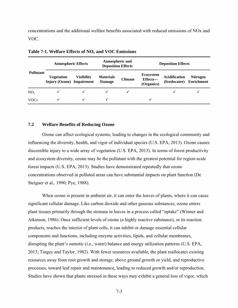
7-3
concentrations and the additional welfare benefits associated with reduced emissions of NOx and
VOC.
Table 7-1. Welfare Effects of NOx and VOC Emissions
Pollutant
Atmospheric Effects Atmospheric and Deposition Effects
Deposition Effects
Vegetation Injury (Ozone)
Visibility Impairment
Materials Damage
Climate Ecosystem Effects—
(Organics)
Acidification (freshwater)
Nitrogen Enrichment
NOx
VOCs
7.2 Welfare Benefits of Reducing Ozone
Ozone can affect ecological systems, leading to changes in the ecological community and
influencing the diversity, health, and vigor of individual species (U.S. EPA, 2013). Ozone causes
discernible injury to a wide array of vegetation (U.S. EPA, 2013). In terms of forest productivity
and ecosystem diversity, ozone may be the pollutant with the greatest potential for region-scale
forest impacts (U.S. EPA, 2013). Studies have demonstrated repeatedly that ozone
concentrations observed in polluted areas can have substantial impacts on plant function (De
Steiguer et al,. 1990; Pye, 1988).
When ozone is present in ambient air, it can enter the leaves of plants, where it can cause
significant cellular damage. Like carbon dioxide and other gaseous substances, ozone enters
plant tissues primarily through the stomata in leaves in a process called “uptake” (Winner and
Atkinson, 1986). Once sufficient levels of ozone (a highly reactive substance), or its reaction
products, reaches the interior of plant cells, it can inhibit or damage essential cellular
components and functions, including enzyme activities, lipids, and cellular membranes,
disrupting the plant’s osmotic (i.e., water) balance and energy utilization patterns (U.S. EPA,
2013; Tingey and Taylor, 1982). With fewer resources available, the plant reallocates existing
resources away from root growth and storage, above ground growth or yield, and reproductive
processes, toward leaf repair and maintenance, leading to reduced growth and/or reproduction.
Studies have shown that plants stressed in these ways may exhibit a general loss of vigor, which

7-4
can lead to secondary impacts that modify plants' responses to other environmental factors.
Specifically, plants may become more sensitive to other air pollutants, or more susceptible to
disease, pest infestation, harsh weather (e.g., drought, frost) and other environmental stresses,
which can all produce a loss in plant vigor in ozone-sensitive species that over time may lead to
premature plant death. Furthermore, there is evidence that ozone can interfere with the
formation of mycorrhizae, an essential symbiotic fungus associated with the roots of most
terrestrial plants, by reducing the amount of carbon available for transfer from the host to the
symbiont (U.S. EPA, 2013).
This ozone damage may or may not be accompanied by visible injury on leaves, and
likewise, visible foliar injury may or may not be a symptom of the other types of plant damage
described above. Foliar injury is usually the first visible sign of injury to plants from ozone
exposure and indicates impaired physiological processes in the leaves (Grulke, 2003). When
visible injury is present, it is commonly manifested as chlorotic or necrotic spots, and/or
increased leaf senescence (accelerated leaf aging). Visible foliar injury reduces the aesthetic
value of ornamental vegetation and trees in urban landscapes and negatively affects scenic vistas
in protected natural areas.
Ozone can produce both acute and chronic injury in sensitive species depending on the
concentration level and the duration of the exposure. Ozone effects also tend to accumulate over
the growing season of the plant, so that even lower concentrations experienced for a longer
duration have the potential to create chronic stress on sensitive vegetation. Not all plants,
however, are equally sensitive to ozone. Much of the variation in sensitivity between individual
plants or whole species is related to the plant’s ability to regulate the extent of gas exchange via
leaf stomata (e.g., avoidance of ozone uptake through closure of stomata) and the relative ability
of species to detoxify ozone-generated reactive oxygen free radicals (U.S. EPA, 2013; Winner,
1994). After injuries have occurred, plants may be capable of repairing the damage to a limited
extent (U.S. EPA, 2013). Because of the differing sensitivities among plants to ozone, ozone
pollution can also exert a selective pressure that leads to changes in plant community
composition. Given the range of plant sensitivities and the fact that numerous other
environmental factors modify plant uptake and response to ozone, it is not possible to identify
threshold values above which ozone is consistently toxic for all plants.
7-5
Because plants are at the base of the food web in many ecosystems, changes to the plant
community can affect associated organisms and ecosystems (including the suitability of habitats
that support threatened or endangered species and below ground organisms living in the root
zone). Ozone impacts at the community and ecosystem level vary widely depending upon
numerous factors, including concentration and temporal variation of tropospheric ozone, species
composition, soil properties and climatic factors (U.S. EPA, 2013). In most instances, responses
to chronic or recurrent exposure in forested ecosystems are subtle and not observable for many
years. These injuries can cause stand-level forest decline in sensitive ecosystems (U.S. EPA,
2013, McBride et al., 1985; Miller et al., 1982). It is not yet possible to predict ecosystem
responses to ozone with certainty; however, considerable knowledge of potential ecosystem
responses is available through long-term observations in highly damaged forests in the U.S. (U.S
EPA, 2013). Biomass loss due to ozone exposure affects climate regulation by reducing carbon
sequestration. More carbon stays in the atmosphere because carbon uptake by forests is reduced.
The studies cited in the Ozone ISA demonstrate a consistent pattern of reduced carbon uptake
because of ozone damage, with some of the largest reductions projected over North America
(U.S. EPA, 2013).
Ozone also directly contributes to climate change because tropospheric ozone traps heat,
leading to increased surface temperatures. Projections of radiative forcing due to changing
ozone concentrations over the 21st century show wide variation, due in large part to the
uncertainty of future emissions of source gases (U.S. EPA 2014a). However, reduction of
tropospheric ozone concentrations could provide an important means to slow climate change in
addition to the added benefit of improving surface air quality (U.S. EPA, 2014a).
While it is clear that increases in tropospheric ozone lead to warming, the precursors of
ozone also have competing effects on methane, complicating emissions reduction strategies. A
decrease in carbon monoxide or VOC emissions would shorten the lifetime of methane, leading
to an overall cooling effect. A decrease in NOX emissions could lengthen the methane lifetime in
certain regions, leading to warming (U.S. EPA, 2014a). Additionally, some strategies to reduce
ozone precursor emissions could also lead to the reduced formation of aerosols (e.g., nitrates and
sulfates) that currently have a cooling effect.

7-6
In the proposal RIA (U.S. EPA, 2014b), we were able to quantify only a small portion of
the welfare impacts associated with reductions in ozone concentrations to meet alternative ozone
standards. Using a model of commercial agriculture and forest markets, we analyzed the effects
on consumers and producers of forest and agricultural products of changes in the W126 index
resulting from meeting alternative standards within the proposed range of 70 to 65 ppb, as well
as a lower standard level of 60 ppb. We also assessed the effects of those changes in commercial
agricultural and forest yields on carbon sequestration and storage. This analysis provided limited
quantitative information on the welfare benefits of meeting these alternative standards, focused
only on one subset of ecosystem services. Commercial and non-commercial forests provide a
number of additional services, including medicinal uses, non-commercial food and fiber
production, arts and crafts uses, habitat, recreational uses, and cultural uses for Native American
tribes. A more complete discussion of these additional ecosystem services is provided in the
final Welfare Risk and Exposure Assessment for Ozone (WREA) (U.S. EPA, 2014a). Because we
did not update this analysis for this RIA, we refer the reader to the results in the proposal RIA for
an indication of the potential magnitude of these welfare benefits.
7.3 Additional Welfare Benefits of Strategies to Meet the Ozone NAAQS
Reductions in emissions of NOx and VOC are associated with additional welfare benefits,
including reductions in nutrient enrichment and acidification impacts on sensitive aquatic and
terrestrial ecosystems and improvements in visibility in state and national parks, wilderness
areas, and in the areas where people live and work.
Excess nitrogen deposition can lead to eutrophication of estuarine waters, which is
associated with a range of adverse ecological effects. These include low dissolved oxygen
(DO), harmful algal blooms (HABs), loss of submerged aquatic vegetation (SAV), and low water
clarity. Low DO disrupts aquatic habitats, causing stress to fish and shellfish, which, in the
short-term, can lead to episodic fish kills and, in the long-term, can damage overall growth in
fish and shellfish populations. HAB are often toxic to fish and shellfish, lead to fish kills and
aesthetic impairments of estuaries, and can in some instances be harmful to human health. SAV
provides critical habitat for many aquatic species in estuaries and, in some instances, can also
protect shorelines by reducing wave strength. Low water clarity is in part the result of

7-7
accumulations of both algae and sediments in estuarine waters. In addition to contributing to
declines in SAV, high levels of turbidity also degrade the aesthetic qualities of the estuarine
environment.
Nutrient enrichment from nitrogen deposition to terrestrial ecosystems is causally linked
to alteration of species richness, species composition, and biodiversity (U.S. EPA, 2008b).
Nitrogen enrichment occurs over a long time period; as a result, it may take as much as 50 years or
more to see changes in ecosystem conditions, indicators, and services.
Terrestrial acidification resulting from deposition of nitrogen can result in declines in
sensitive tree species, such as red spruce (Picea rubens) and sugar maple (Acer saccharum), and
can also impact other plant communities including shrubs and lichen (U.S. EPA, 2008b).
Biological effects of acidification in terrestrial ecosystems are generally linked to aluminum
toxicity and decreased ability of plant roots to take up base cations (U.S. EPA, 2008b).
Terrestrial acidification affects several important ecosystem services, including declines in
habitat for threatened and endangered species, declines in forest aesthetics and productivity, and
increases in forest soil erosion and reductions in water retention.
Aquatic acidification resulting from deposition of nitrogen can result in effects on health,
vigor, and reproductive success for aquatic species; and effects on biodiversity. Deposition of
nitrogen results in decreases in the acid neutralizing capacity and increases in inorganic aluminum
concentration, which contribute to declines in zooplankton, macro invertebrates, and fish species
richness in aquatic ecosystems (U.S. EPA, 2008b).
Reductions in NOx emissions will improve visibility in parks and wilderness areas and in
places where people live and work because of their impact on light extinction (U.S. EPA, 2009).
Good visibility increases quality of life where individuals live and work, and where they travel
for recreational activities, including sites of unique public value, such as the Great Smoky
Mountains National Park (U. S. EPA, 2009). Particulate nitrate is an important contributor to
light extinction in California and the upper Midwestern U.S., particularly during winter (U.S.
EPA, 2009). While EPA typically estimates the visibility benefits associated with reductions in NOx
(U.S. EPA, 2008a), we have not done so here because we do not have estimates of the changes in

7-8
particulate nitrate needed to calculate changes in light extinction and the resulting changes in
economic benefits.
Strategies implemented by state and local governments to reduce emissions of ozone
precursors may also impact emissions of CO2 or other long-lived climate gases. Our ability to
quantify the climate effects of the proposed standard levels is limited due to lack of available
information on the energy and associated climate gas implications of control technologies
assumed in the illustrative control strategy alternatives, remaining uncertainties regarding the
impact of ozone precursors on climate change, and lack of available information on the co-
controlled greenhouse gas (GHG) emission reductions. As a result, we do not attempt to
quantify the impacts of the illustrative attainment scenarios on GHG emissions and impacts.
7.4 References
De Steiguer, J., Pye, J., Love, C. 1990. Air Pollution Damage to U.S. Forests. Journal of Forestry, 88(8), 17-22.
Grulke, N.E. 2003. The physiological basis of ozone injury assessment attributes in Sierran conifers. In A. Bytnerowicz, M.J. Arbaugh, & R. Alonso (Eds.), Ozone air pollution in the Sierra Nevada: Distribution and effects on forests. (pp. 55-81). New York, NY: Elsevier Science, Ltd.
McBride, J.R., Miller, P.R., Laven, R.D. 1985. Effects of oxidant air pollutants on forest succession in the mixed conifer forest type of southern California. In: Air Pollutants Effects on Forest Ecosystems, Symposium Proceedings, St. P, 1985, p. 157-167.
Millennium Ecosystem Assessment Board (MEA). 2005. Ecosystems and Human Well-being: Synthesis. Washington, DC: World Resources Institute. Available on the Internet at <http://www.who.int/globalchange/ecosystems/ecosystems05/en/index.html>.
Miller, P.R., O.C. Taylor, R.G. Wilhour. 1982. Oxidant air pollution effects on a western coniferous forest ecosystem. Corvallis, OR: U.S. Environmental Protection Agency, Environmental Research Laboratory (EPA600-D-82-276).
Pye, J.M. 1988. Impact of ozone on the growth and yield of trees: A review. Journal of Environmental Quality, 17, 347-360.
Tingey, D.T., and Taylor, G.E. 1982. Variation in plant response to ozone: a conceptual model of physiological events. In M.H. Unsworth & D.P. Omrod (Eds.), Effects of Gaseous Air Pollution in Agriculture and Horticulture. (pp.113-138). London, UK: Butterworth Scientific.
U.S. Environmental Protection Agency (U.S. EPA). 2006. Ecological Benefits Assessment Strategic Plan. EPA-240-R-06-001. Office of the Administrator. Washington, DC. October. Available on the Internet at <http://yosemite.epa.gov/ee/epa/eed.nsf/webpages/EcologBenefitsPlan.html>.
U.S. Environmental Protection Agency (U.S. EPA). 2008a. Regulatory Impact Analysis, 2008 National Ambient Air Quality Standards for Ground-level Ozone, Chapter 6. Office of Air Quality Planning and Standards, Research Triangle Park, NC. March. Available at <http://www.epa.gov/ttn/ecas/regdata/RIAs/6-ozoneriachapter6.pdf>.

7-9
U.S. Environmental Protection Agency (U.S. EPA). 2008b. Integrated Science Assessment for Oxides of Nitrogen and Sulfur—Ecological Criteria National (Final Report). National Center for Environmental Assessment, Research Triangle Park, NC. EPA/600/R-08/139. December. Available on the Internet at <http://cfpub.epa.gov/ncea/cfm/recordisplay.cfm?deid=201485>.
U.S. Environmental Protection Agency (U.S. EPA). 2009. Integrated Science Assessment for Particulate Matter (Final Report). EPA-600-R-08-139F. National Center for Environmental Assessment—RTP Division. December. Available on the Internet at <http://cfpub.epa.gov/ncea/cfm/recordisplay.cfm?deid=216546>.
U.S. Environmental Protection Agency (U.S. EPA). 2013. Integrated Science Assessment of Ozone and Related Photochemical Oxidants (Final Report). EPA-600/R-10/076F. February. Available on the Internet at <http://cfpub.epa.gov/ncea/isa/recordisplay.cfm?deid=247492>.
U.S. EPA. (U.S. Environmental Protection Agency). 2014a. Welfare Risk and Exposure Assessment (Final). August. Available on the internet at: <http://www.epa.gov/ttn/naaqs/standards/ozone/data/20141021welfarerea.pdf>.
U.S. Environmental Protection Agency (U.S. EPA). 2014b. Regulatory Impact Analysis of the Proposed Revisions
to the National Ambient Air Quality Standards for Ground-Level Ozone. Office of Air Quality Planning and Standards, Research Triangle Park, NC. November. Available at <http://www.epa.gov/ttnecas1/regdata/RIAs/20141125ria.pdf >.
Winner, W.E. 1994. Mechanistic analysis of plant responses to air pollution. Ecological Applications, 4(4), 651-661.
Winner, W.E., and C.J. Atkinson. 1986. Absorption of air pollution by plants, and consequences for growth. Trends in Ecology and Evolution 1:15-18.

8-1
CHAPTER 8: COMPARISON OF COSTS AND BENEFITS
Overview
The EPA performed an illustrative analysis to estimate the costs and human health
benefits of nationally attaining revised and alternative ozone standards. The EPA Administrator
is revising the level of the primary ozone standard to 70 ppb. Per Executive Order 12866 and the
guidelines of OMB Circular A-4, this Regulatory Impact Analysis (RIA) presents analysis of an
alternative standard level of 65 ppb. This chapter summarizes these results and discusses the
implications of the analysis. The cost and benefit estimates below are calculated incremental to a
2025 baseline assuming attainment of the existing ozone standard of 75 ppb and incorporating air
quality improvements achieved through the projected implementation of existing regulations.
8.1 Results
In this RIA we present the primary cost and benefit estimates for full attainment in 2025.
For analytical purposes, we assume that almost all areas of the country will meet each alternative
standard level in 2025 through the adoption of technologies at least as effective as the control
strategies used in this illustration. It is expected that some costs and benefits will begin
occurring earlier, as states begin implementing control measures to attain earlier or to show
progress towards attainment. For California, we provide estimates of the costs and benefits of
attaining the standard in a post-2025 time frame.
In estimating the incremental costs and benefits of the revised and alternative standard
levels, we recognize that there are several areas that are not required to meet the existing ozone
standard by 2025. The Clean Air Act allows areas with more significant air quality problems to
take additional time to reach the existing standard. Several areas in California are not required to
meet the existing standard by 2025, and depending on how areas are ultimately designated for a
revised standard, many areas may not be required to meet a revised standard until sometime
between 2032 and December 31, 2037. Because of data and resource constraints, we were not
able to project emissions and air quality beyond 2025 for California; however, we adjusted
baseline air quality to reflect mobile source emissions reductions for California that would occur
between 2025 and 2030; these emissions reductions will be the result of mobile source
8-2
regulations expected to be fully implemented by 2030. While there is uncertainty about the
precise timing of emissions reductions and related costs for California, we assume costs occur
through the end of 2037 and beginning of 2038. In addition, we model benefits for California
using projected population demographics for 2038.
Because of the different timing for incurring costs and accruing benefits and for ease of
discussion throughout the analyses, we refer to the different time periods for potential attainment
as 2025 and post-2025 to reflect that (1) we did not project emissions and air quality for any year
other than 2025; (2) for California, emissions controls and associated costs are assumed to occur
through the end of 2037 and beginning of 2038; and (3) for California benefits are modeled using
population demographics in 2038. It is not straightforward to discount the post-2025 results for
California to compare with or add to the 2025 results for the rest of the U.S. While we estimate
benefits using 2038 information, we do not have good information on precisely when the costs of
controls will be incurred. Because of these differences in timing related to California attaining a
revised standard, the separate post-2025 costs and benefits estimates for California should not be
added to the primary 2025 estimates for the rest of the U.S.
By the 2030s, various mobile source rules, such as the onroad and nonroad diesel rules,
are expected to be fully implemented. Because California will likely not have all of its areas in
attainment with a revised standard until sometime after its attainment date for the existing
standard, it is important to reflect the impact these mobile source rules might have on the
emissions that affect ozone nonattainment. To reflect the emissions reductions that are expected
from these rules, we subtract them from the estimates of the emissions reductions that might be
needed for California to fully attain in 2025, making our analysis more consistent with full
attainment later than 2025. The EPA did the analysis this way to be consistent with the
requirements in the Clean Air Act and because forcing full attainment in California in an earlier
year would likely lead to overstating costs and benefits due to (1) emissions reductions those
areas might enjoy from existing federal or state programs implemented between 2025 and the
future potential attainment year, (2) the likelihood that energy efficiency and cleaner
technologies will be further implemented, and/or (3) the potential decline in costs of existing
technologies due to economies of scale or improvements in the efficiency of installing and
operating controls (‘learning by doing’).

8-3
Tables 8-1 and 8-2 summarize the total costs and benefits of the revised and alternative
standard levels analyzed, and show the net benefits for each of the levels across a range of
modeling assumptions related to the calculation of costs and benefits.175 Tables 8-3 and 8-4
summarize the costs and benefits resulting from identified control strategies and do not include
the additional costs and benefits associated with the unidentified control strategies. Tables 8-5
and 8-6 provide information on the total costs by geographic region for the U.S., except
California in 2025 and on the costs for California for post-2025. Tables 8-7 and 8-8 provide a
regional breakdown of benefits for 2025 and a regional breakdown of benefits for post-2025.
The estimates for benefits reflect the variability in the functions available for estimating
the largest source of benefits – avoided premature mortality associated with simulated reductions
in ozone and PM2.5 (as a co-benefit). The low end of the range of net benefits is constructed by
subtracting the cost from the lowest benefit, while the high end of the range is constructed by
subtracting the cost from the highest benefit. Following these tables is a discussion of the
implications of these estimates, as well as the uncertainties and limitations that should be
considered in interpreting the estimates.
In the RIA we provide estimates of costs of emissions reductions to attain the revised and
alternative standards in three regions -- California, the rest of the western U.S., and the eastern
U.S. In addition, we provide estimates of the benefits that accrue to each of these three regions
resulting from both control strategies applied within the region and reductions in transport of
ozone associated with emissions reductions in other regions.
The net benefits of emissions reductions strategies in a specific region would be the
benefits of the emissions reductions occurring both within and outside of the region minus the
costs of the emissions reductions. Because the air quality modeling is done at the national level,
we do not estimate separately the nationwide benefits associated with the emissions reductions
175 As discussed in Chapter 2, Section 2.2.5, of the 1,225 ozone monitors with complete ozone data, there were seven monitors, or 0.6 percent of the total, for which the DVs were influenced by wintertime ozone episodes. These seven monitors were removed from the analysis because the modeling tools are not currently sufficient to properly characterize ozone formation during wintertime ozone episodes. Because there was no technically feasible method for projecting DVs at these sites, these sites were not included in determining required NOx and VOC emissions reductions needed to meet the revised or alternative standard levels. There could be additional emissions reductions required to lower ozone at these locations and associated additional costs and benefits not reflected in this analysis.

8-4
occurring in any specific region.176 As a result, we are only able to provide net benefits
estimates at the national level. The difference between the estimated benefits accruing to a
specific region and the costs for that region is not an estimate of net benefits of the emissions
reductions in that region because it ignores the benefits occurring outside of that region.
Table 8-1. Total Costs, Total Monetized Benefits, and Net Benefits of Control Strategies in 2025 for U.S., except California (billions of 2011$)a,b
Revised and Alternative
Standard Levels
Total Costsc Monetized Benefits Net Benefits7% Discount
Rate 7% Discount
Rate 7% Discount
Rate 70 $1.4 $2.9 to $5.9d $1.5 to $4.5 65 $16 $15 to $30d -$1.0 to $14
a All values are rounded to two significant figures. b Estimating multiple years of costs and benefits is not possible for this RIA due to data and resource limitations. As a result, we provide a snapshot of costs and benefits in 2025, using the best available information to approximate social costs and social benefits recognizing uncertainties and limitations in those estimates. c The numbers presented in this table reflect engineering costs annualized at a 7 percent discount rate to the extent possible. d Excludes additional health and welfare benefits that could not be quantified (see Chapter 6, Section 6.6.3.8).
Table 8-2. Total Costs, Total Monetized Benefits, and Net Benefits of Control Strategies Applied in California, Post-2025 (billions of 2011$)a
Revised and Alternative
Standard Levels
Total Costs Monetized Benefits Net Benefits 7% Discount
Rate 7% Discount
Rate 7% Discount
Rate 70 $0.8 $1.2 to $2.1c $0.4 to $1.3
65 $1.5 $2.3 to $4.2c $0.8 to $2.7 a Estimating multiple years of costs and benefits is not possible for this RIA due to data and resource limitations. As a result, we provide a snapshot of costs and benefits in 2025, using the best available information to approximate social costs and social benefits recognizing uncertainties and limitations in those estimates. b The numbers presented in this table reflect engineering costs annualized at a 7 percent discount rate to the extent possible. c Excludes additional health and welfare benefits that could not be quantified (see Chapter 6, Section 6.6.3.8).
176 For California, we provide separate estimates of the costs and nationwide estimates of benefits, so it is appropriate to calculate net benefits. As such, we provide net benefits for the post-2025 California analysis.
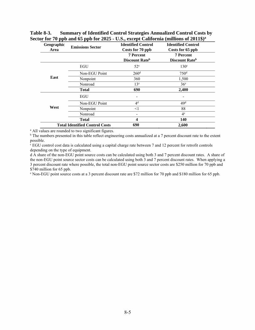
8-5
Table 8-3. Summary of Identified Control Strategies Annualized Control Costs by Sector for 70 ppb and 65 ppb for 2025 - U.S., except California (millions of 2011$)a
Geographic Area
Emissions Sector Identified Control Costs for 70 ppb
Identified Control Costs for 65 ppb
7 Percent
Discount Rateb7 Percent
Discount Rateb
East
EGU 52c 130c
Non-EGU Point 260d 750d Nonpoint 360 1,500 Nonroad 13e 36e Total 690 2,400
West
EGU - -
Non-EGU Point 4d 49d Nonpoint <1 88 Nonroad - 4e Total 4 140
Total Identified Control Costs 690 2,600 a All values are rounded to two significant figures. b The numbers presented in this table reflect engineering costs annualized at a 7 percent discount rate to the extent possible. c EGU control cost data is calculated using a capital charge rate between 7 and 12 percent for retrofit controls depending on the type of equipment. d A share of the non-EGU point source costs can be calculated using both 3 and 7 percent discount rates. A share of the non-EGU point source sector costs can be calculated using both 3 and 7 percent discount rates. When applying a 3 percent discount rate where possible, the total non-EGU point source sector costs are $250 million for 70 ppb and $740 million for 65 ppb. e Non-EGU point source costs at a 3 percent discount rate are $72 million for 70 ppb and $180 million for 65 ppb.

8-6
Table 8-4. Estimated Monetized Ozone and PM2.5 Benefits for Revised and Alternative Annual Ozone Standards Incremental to the Baseline for the 2025 Scenario (Nationwide Benefits of Attaining the Standards in the U.S. except California) – Identified Control Strategies (billions of 2011$) a
Discount
Rate Revised and Alternative Standard Levels
70 ppb 65 ppb Identified Control Strategies Ozone-only Benefits (range reflects Smith et al. (2009) to Zanobetti and Schwartz (2008))
b $0.86 to $1.4 $2.2 to $3.5
PM2.5 Co-benefits (range reflects Krewski et al. (2009) to Lepeule et al. (2012)
3% $1.7 to $3.9 $4.0 to $9.0 7% $1.6 to $3.5 $3.6 to $8.1
Total Benefits 3% $2.6 to $5.3c $6.1 to $12c 7% $2.4 to $4.9c $5.7 to $12c
a Rounded to two significant figures. The reduction in premature fatalities each year accounts for over 98% of total monetized benefits in this analysis. Mortality risk valuation for PM2.5 assumes discounting over the SAB-recommended 20-year segmented lag structure. Not all possible benefits are quantified and monetized in this analysis. B is the sum of all unquantified health and welfare co-benefits. Data limitations prevented us from quantifying these endpoints, and as such, these benefits are inherently more uncertain than those benefits that we were able to quantify. These estimates reflect the economic value of avoided morbidities and premature deaths using risk coefficients from the studies noted. b Ozone-only benefits reflect short-term exposure impacts and as such are assumed to occur in the same year as ambient ozone reductions. Consequently, social discounting is not applied to the benefits for this category. c Excludes additional health and welfare benefits that could not be quantified (see Chapter 6, Section 6.6.3.8). Table 8-5. Summary of Total Control Costs (Identified + Unidentified) by Revised and
Alternative Standard Level for 2025 - U.S., except California (millions of 2011$, 7% Discount Rate)a
Revised and Alternative Level
Geographic Area
Identified Control Costs
Unidentified Control Costs
Total Control Costs
(Identified and Unidentified)
70 ppb
East 690 700 1,400 West 4 - <5 Total $690 $700 $1,400
65 ppb East 2,400 12,000 15,000 West 140 610 750 Total $2,600 $12,600 $16,000
a All values are rounded to two significant figures. Unidentified control costs are based on an average cost-per-ton methodology described in Chapter 4.
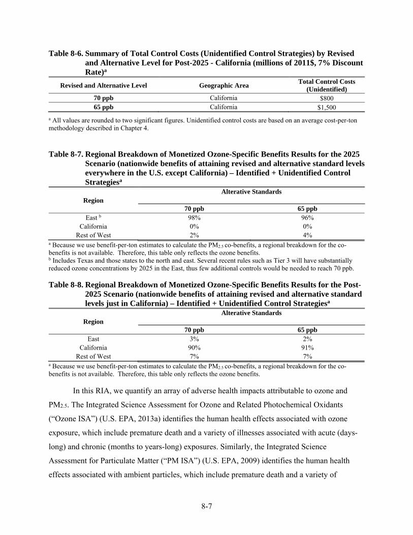
8-7
Table 8-6. Summary of Total Control Costs (Unidentified Control Strategies) by Revised and Alternative Level for Post-2025 - California (millions of 2011$, 7% Discount Rate)a
Revised and Alternative Level Geographic Area Total Control Costs
(Unidentified) 70 ppb California $800 65 ppb California $1,500
a All values are rounded to two significant figures. Unidentified control costs are based on an average cost-per-ton methodology described in Chapter 4.
Table 8-7. Regional Breakdown of Monetized Ozone-Specific Benefits Results for the 2025
Scenario (nationwide benefits of attaining revised and alternative standard levels everywhere in the U.S. except California) – Identified + Unidentified Control Strategiesa
Region Alterative Standards
70 ppb 65 ppb East b 98% 96%
California 0% 0% Rest of West 2% 4%
a Because we use benefit-per-ton estimates to calculate the PM2.5 co-benefits, a regional breakdown for the co-benefits is not available. Therefore, this table only reflects the ozone benefits. b Includes Texas and those states to the north and east. Several recent rules such as Tier 3 will have substantially reduced ozone concentrations by 2025 in the East, thus few additional controls would be needed to reach 70 ppb. Table 8-8. Regional Breakdown of Monetized Ozone-Specific Benefits Results for the Post-
2025 Scenario (nationwide benefits of attaining revised and alternative standard levels just in California) – Identified + Unidentified Control Strategiesa
Region Alterative Standards
70 ppb 65 ppb East 3% 2%
California 90% 91% Rest of West 7% 7%
a Because we use benefit-per-ton estimates to calculate the PM2.5 co-benefits, a regional breakdown for the co-benefits is not available. Therefore, this table only reflects the ozone benefits.
In this RIA, we quantify an array of adverse health impacts attributable to ozone and
PM2.5. The Integrated Science Assessment for Ozone and Related Photochemical Oxidants
(“Ozone ISA”) (U.S. EPA, 2013a) identifies the human health effects associated with ozone
exposure, which include premature death and a variety of illnesses associated with acute (days-
long) and chronic (months to years-long) exposures. Similarly, the Integrated Science
Assessment for Particulate Matter (“PM ISA”) (U.S. EPA, 2009) identifies the human health
effects associated with ambient particles, which include premature death and a variety of

8-8
illnesses associated with acute and chronic exposures. Air pollution can affect human health in a
variety of ways, and in Table 8-9 we summarize the “categories” of effects and describe those
that we could quantify in our “core” benefits estimates and those we were unable to quantify
because we lacked the data, time or techniques.
Table 8-9. Human Health Effects of Pollutants Potentially Affected by Strategies to Attain the Primary Ozone Standards
Benefits Category Specific Effect Effect Has
Been Quantified
Effect Has Been
Monetized
More Information
Improved Human Health Reduced incidence of premature mortality from exposure to ozone
Premature mortality based on short-term exposure (all ages)
Section 5.6
Premature respiratory mortality based on long-term exposure (age 30–99)
a Section 5.6
Reduced incidence of morbidity from exposure to ozone
Hospital admissions—respiratory causes (age > 65)
Section 5.6
Emergency department visits for asthma (all ages)
Section 5.6
Asthma exacerbation (age 6-18) Minor restricted-activity days (age 18–65) Section 5.6 School absence days (age 5–17) Section 5.6 Decreased outdoor worker productivity (age 18–65)
a a Section 5.6
Other respiratory effects (e.g., mediation use, pulmonary inflammation, decrements in lung functioning)
— — ozone ISA c
Cardiovascular (e.g., hospital admissions, emergency department visits)
— — ozone ISA c
Reproductive and developmental effects (e.g., reduced birthweight, restricted fetal growth)
— — ozone ISA c
Reduced incidence of premature mortality from exposure to PM2.5
Adult premature mortality based on cohort study estimates and expert elicitation estimates (age >25 or age >30)
Section 5.6 of PM RIA
Infant mortality (age <1) Section 5.6 of PM RIA
Reduced incidence of morbidity from exposure to PM2.5
Non-fatal heart attacks (age > 18) Section 5.6 of PM RIA
Hospital admissions—respiratory (all ages)
Section 5.6 of PM RIA
Hospital admissions—cardiovascular (age >20)
Section 5.6 of PM RIA
Emergency department visits for asthma (all ages)
Section 5.6 of PM RIA
Acute bronchitis (age 8–12) Section 5.6 of PM RIA
Lower respiratory symptoms (age 7–14) Section 5.6 of PM RIA
Upper respiratory symptoms (asthmatics age 9–11)
Section 5.6 of PM RIA
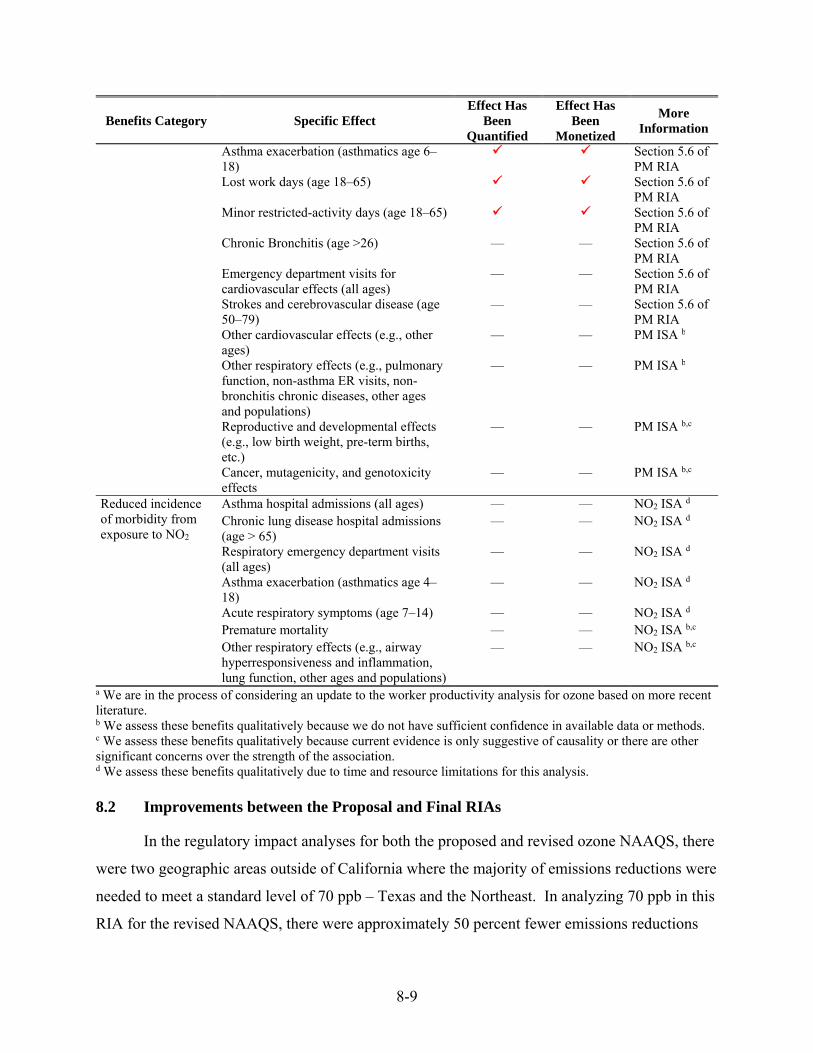
8-9
Benefits Category Specific Effect Effect Has
Been Quantified
Effect Has Been
Monetized
More Information
Asthma exacerbation (asthmatics age 6–18)
Section 5.6 of PM RIA
Lost work days (age 18–65) Section 5.6 of PM RIA
Minor restricted-activity days (age 18–65) Section 5.6 of PM RIA
Chronic Bronchitis (age >26) — — Section 5.6 of PM RIA
Emergency department visits for cardiovascular effects (all ages)
— — Section 5.6 of PM RIA
Strokes and cerebrovascular disease (age 50–79)
— — Section 5.6 of PM RIA
Other cardiovascular effects (e.g., other ages)
— — PM ISA b
Other respiratory effects (e.g., pulmonary function, non-asthma ER visits, non-bronchitis chronic diseases, other ages and populations)
— — PM ISA b
Reproductive and developmental effects (e.g., low birth weight, pre-term births, etc.)
— — PM ISA b,c
Cancer, mutagenicity, and genotoxicity effects
— — PM ISA b,c
Reduced incidence of morbidity from exposure to NO2
Asthma hospital admissions (all ages) — — NO2 ISA d Chronic lung disease hospital admissions (age > 65)
— — NO2 ISA d
Respiratory emergency department visits (all ages)
— — NO2 ISA d
Asthma exacerbation (asthmatics age 4–18)
— — NO2 ISA d
Acute respiratory symptoms (age 7–14) — — NO2 ISA d Premature mortality — — NO2 ISA b,c Other respiratory effects (e.g., airway hyperresponsiveness and inflammation, lung function, other ages and populations)
— — NO2 ISA b,c
a We are in the process of considering an update to the worker productivity analysis for ozone based on more recent literature. b We assess these benefits qualitatively because we do not have sufficient confidence in available data or methods. c We assess these benefits qualitatively because current evidence is only suggestive of causality or there are other significant concerns over the strength of the association. d We assess these benefits qualitatively due to time and resource limitations for this analysis. 8.2 Improvements between the Proposal and Final RIAs
In the regulatory impact analyses for both the proposed and revised ozone NAAQS, there
were two geographic areas outside of California where the majority of emissions reductions were
needed to meet a standard level of 70 ppb – Texas and the Northeast. In analyzing 70 ppb in this
RIA for the revised NAAQS, there were approximately 50 percent fewer emissions reductions

8-10
needed in these two geographic areas. For an alternative standard of 65 ppb, emissions
reductions needed nationwide were approximately 20 percent lower than at proposal.
The primary reason for the difference in emissions reductions estimated for attainment is
that for this RIA we conducted more geographically-refined air quality sensitivity modeling to
develop improved ozone response factors (see Chapter 2, Section 2.1.4 for a more detailed
discussion of this air quality modeling) and focused the emissions reduction strategies on
geographic areas closer to the monitors with the highest design values (see Chapter 3, Section
3.1.2 for a more detailed discussion of the emissions reduction strategies). The improvements in
air quality modeling and emissions reduction strategies account for about 80 percent of the
difference in needed emissions reductions between the two RIAs.
In Texas and the Northeast, the updated response factors and more focused emissions
reduction strategies resulted in larger changes in ozone concentrations in response to more
geographically focused emissions reductions. In east Texas, the ppb/ton ozone response factors
used in this RIA were 2 to 3 times more responsive than the factors used in the proposal RIA at
controlling monitors in Houston and Dallas. In the Northeast, the ppb/ton ozone response factors
used in this RIA were 2.5 times more responsive than the factors used in the proposal RIA at the
controlling monitor on Long Island, NY.
A secondary reason for the difference is that in the time between developing the two
RIAs we updated emissions inventories, models and model inputs for the base year of 2011. See
Chapter 2, Section 2.1 and 2.2 for additional discussion of the updated emissions inventories,
models and model inputs. When projected to 2025, these changes in inventories, models and
inputs had compounding effects for year 2025, and in some areas resulted in lower projected
base case design values for 2025. The updated emissions inventories, models, and model inputs
account for about 20 percent of the difference in needed emissions reductions between the two
RIAs.
These differences in the estimates of emissions reductions needed to attain the revised
and alternative standard levels affect the estimates for the costs and benefits in this RIA. For a
revised standard of 70 ppb, the costs were 60 percent lower than at proposal and the benefits
were 55 percent lower than at proposal. The percent decrease in costs is slightly more than the

8-11
percent decrease in emissions reductions because a larger number of lower cost identified
controls were available to bring areas into attainment with 70 ppb.177 The percent decrease in
benefits is similar to the percent decrease in emissions reductions. For an alternative standard
level of 65 ppb, the costs were less than three percent higher than those estimated at proposal and
the benefits were 22 percent lower than at proposal.178 The percent change in costs was less than
the percent decrease in emissions reductions because in this analysis we applied identified
controls in smaller geographic areas, resulting in fewer identified controls available within those
areas and an increase in higher cost unidentified controls being applied to bring areas into
attainment with 65 ppb. The percent decrease in benefits is similar to the percent decrease in
emissions reductions.
8.2.1 Relative Contribution of PM Benefits to Total Benefits
Because of the relatively strong relationship between PM2.5 concentrations and premature
mortality, PM co-benefits resulting from reductions in NOx emissions can make up a large
fraction of total monetized benefits, depending on the specific PM mortality impact function
used, and on the relative magnitude of ozone benefits, which is dependent on the specific ozone
mortality function assumed. PM co-benefits based on daily average concentrations are
calculated over the entire year, while ozone related benefits are calculated only during the
summer ozone season. Because the control strategies evaluated in this RIA are assumed to
operate year round rather than only during the ozone season, this means that PM benefits will
accumulate during both the ozone season and the rest of the year. For primary benefits estimates
in 2025, PM2.5 co-benefits account for approximately half to three-quarters of the estimated
benefits, depending on the standard analyzed and on the choice of ozone and PM mortality
functions used.
177 In the final RIA, outside of California all areas were projected to meet the current standard of 75 ppb. As such, no identified controls were used to bring areas into attainment with 75 ppb. In the proposal RIA, some of these lower cost controls were used to bring areas into attainment with 75 ppb, making them unavailable for application in the analysis of 70 ppb. 178 We have slightly modified our approach to estimating morbidity benefits since proposal, which had a negligible (~1%) influence on the total monetized benefits in this RIA.

8-12
8.2.2 Developing Future Control Strategies with Limited Data
Because of relatively higher ozone levels in several large urban areas (Southern
California, Houston, and the Northeastern urban corridor, including New York and Philadelphia)
and because of limitations associated with the data on currently identified emissions control
technologies, the EPA recognized that identified and reasonably anticipated emissions controls
would likely not be sufficient to bring some areas into attainment with either the existing or
alternative, more stringent ozone standard level. Therefore, we designed this analysis in two
stages: the first stage focused on analyzing the air quality improvements that could be achieved
through application of documented, well-characterized, end-of-pipe emissions controls, and the
costs and benefits associated with those controls. The second stage took the emissions
reductions beyond identified controls and used an average cost-per-ton method to estimate the
costs and benefits of these additional emissions reductions needed to bring all areas into full
attainment with the alternative standard levels analyzed.
The structure of the RIA reflects this two-stage analytical approach. Separate chapters are
provided for the emissions, air quality, and cost impacts of identified controls. We used the
information currently available to develop reasonable approximations of the costs and benefits of
the unidentified portion of the emissions reductions necessary to reach attainment. However,
because of the uncertainty associated with the costs of unidentified controls, we judged it
appropriate to provide separate estimates of the costs and benefits for partial attainment (based
on identified controls) and full attainment (based on identified controls and unidentified
controls), as well as an overall estimate for reaching full attainment. There is a single chapter on
benefits, because the methodology for estimating benefits does not change between stages.
However, in that chapter, we again provide separate estimates of the benefits associated with the
partial attainment and full attainment portions of the analysis.
In both stages of the analysis, it should be recognized that all estimates of future costs and
benefits are not intended to be forecasts of the actual costs and benefits of implementing
potentially revised standards. Ultimately, states and local areas will be responsible for
developing and implementing emissions control programs to reach attainment with the ozone
NAAQS, with the timing of attainment being determined by future decisions by states and the
EPA. Our estimates are intended to provide information on the general magnitude of the costs
8-13
and benefits of alternative standard levels rather than on precise predictions of control measures,
costs, or benefits. With these caveats, we expect that this analysis can provide a reasonable
picture of the types of emissions controls that are currently available, the direct costs of those
controls, the levels of emissions reductions that may be achieved with these controls, the air
quality impact that can be expected to result from reducing emissions, and the public health
benefits of reductions in ambient ozone levels. This analysis identifies those areas of the U.S.
where our existing knowledge of control strategies is not sufficient to allow us to model
attainment, and where additional data or research may be needed to develop strategies for
attainment.
In many ways, RIAs for proposed and final actions are learning processes that can yield
valuable information about the technical and policy issues that are associated with a particular
regulatory action. This is especially true for RIAs for proposed and revised NAAQS, where we
are required to stretch our understanding of both science and technology to develop scenarios
that illustrate how certain we are about how economically feasible the attainment of these
standards might be regionally. The ozone NAAQS RIA provided great challenges when
compared to previous RIAs primarily because as we tighten standards across multiple pollutants
with overlapping precursors (e.g., the recent tightening of the PM2.5 standards), we move further
down the list of cost-effective identified and available controls in our database. With the more
stringent NAAQS, more areas will need to employ additional ways of reducing emissions. The
control measures reflected in our databases include very few abatement possibilities from energy
efficiency measures, fuel switching, input or process changes, or other abatement strategies that
are non-traditional in the sense that they are not the application of an end-of-pipe control. So
while we can speculate on what some of the future emissions reduction strategies might look like
based on new developments in energy efficiency and clean technology, the specific technological
path in different nonattainment areas is not clear.
Because of the uncertainty regarding the development of future emissions reduction
strategies, a significant portion of the analysis is based on extrapolating from available data on
identified control technologies to generate the emissions reductions necessary to reach full
attainment of an alternative ozone NAAQS and the resulting costs and benefits. Studies indicate
that it is not uncommon for pre-regulatory cost estimates to be higher than later estimates, in part
8-14
because of difficulty in predicting technological changes. Over longer time horizons, such as the
time allowed for areas with high levels of ozone pollution to meet the ozone NAAQS, the
opportunity for technical change is greater (See Chapter 4, Section 4.2.3 for additional
discussion). Also, because of the nature of the extrapolation method for benefits (which focuses
on reductions in ozone only at monitors that exceed the NAAQS), we generally understate the
total benefits that would result from implementing additional emissions controls to fully attain
the ozone NAAQS (i.e., assuming that the application of control strategies would result in ozone
reductions both at nonattainment and attainment monitors). On the other hand, the possibility
also exists that benefits are overestimated, because it is possible that new technical changes
might not meet the specifications, development time lines, or cost estimates provided in this
analysis.
8.3 Net Present Value of a Stream of Costs and Benefits
The EPA believes that providing comparisons of social costs and social benefits at
discount rates of 3 and 7 percent is appropriate. The three different uses of discounting in the
RIA – (i) construction of annualized engineering costs, (ii) adjusting the value of mortality risk
for lags in mortality risk decreases, and (iii) adjusting the cost of illness for non-fatal heart
attacks to adjust for lags in follow up costs -- are all appropriate. Our estimates of net benefits
are the approximations of the net value (in 2025) of benefits attributable to emissions reductions
needed to attain just for the year 2025.
The EPA presents annualized costs and benefits in a single year for comparison in this RIA
because there are a number of methodological complexities associated with calculating the net
present value (NPV) of a stream of costs and benefits for a NAAQS. While NPV analysis allows
evaluation of alternatives by summing the present value of all future costs and benefits, insights
into how costs will occur over time are limited by underlying assumptions and data. Calculating
a present value (PV) of the stream of future benefits also poses special challenges, which we
describe below. In addition, the method requires definition of the length of that future time
period, which is not straightforward for this analysis and subject to uncertainty.
To estimate engineering costs, the EPA employs the equivalent uniform annual cost
(EUAC) method, which annualizes costs over varying lifetimes of control measures applied in

8-15
the analysis.179 Using the EUAC method results in a stream of annualized costs that is equal for
each year over the lifetime of control measures, resulting in a value similar to the value
associated with an amortized mortgage or other loan payment. Control equipment is often
purchased by incurring debt rather than through a single up-front payment. Recognizing this led
the EPA to estimate costs using the EUAC method instead of a method that mimics firms paying
up front for the future costs of installation, maintenance, and operation of pollution control
devices.
Further, because we do not know when a facility will stop using a control measure or
change to another measure based on economic or other reasons, the EPA assumes the control
equipment and measures applied in the illustrative control strategies remain in service for their
full useful life. As a result, the annualized cost of controls in a single future year is the same
throughout the lifetimes of control measures analyzed, allowing the EPA to compare the
annualized control costs with the benefits in a single year for consistent comparison.
The EPA’s RIAs for air quality rules generally report the estimated net benefits of
improved air quality for a single year. The estimated NPV can better characterize the stream of
benefits and costs over a multi-year period. However, calculating the PV of improved air quality
is generally quite data-intensive and costly. Further, the results are sensitive to assumptions
regarding the time period over which the stream of benefits is discounted.
The theoretically appropriate approach for characterizing the PV of benefits is the life table
approach. The life table, or dynamic population, approach explicitly models the year-to-year
influence of air pollution on baseline mortality risk, population growth and the birth rate—
typically for each year over the course of a 50-to-100 year period (U.S. EPA SAB, 2010; Miller,
2003). In contrast to the pulse approach180, a life table models these variables endogenously by
following a population cohort over time. For example, a life table will “pass” the air pollution-
modified baseline death rate and population from year to year; impacts estimated in year 50 will
179 See Chapter 4, Section 4.1.1 for additional information on the EUAC method. 180 The pulse approach assumes changes in air pollution in a single year and affects mortality estimates over a 20-year period.

8-16
account for the influence of air pollution on death rates and population growth in the preceding
49 years.
Calculating year-to-year changes in mortality risk in a life table requires some estimate of
the annual change in air quality levels. It is both impractical to model air quality levels for each
year and challenging to account for changes in federal, state and local policies that will affect the
annual level and distribution of pollutants. For each of these reasons the EPA has not generally
reported the PV of benefits for air rules but has instead pursued a pulse approach. While we
agree that providing the NPV of a stream of costs and benefits could be informative, based on
these reasons we are not able to provide the NPV of that stream in this RIA.
8.4 Framing Uncertainty
This section includes a qualitative presentation of key factors that (1) could impact how
air quality changes over time; (2) could impact the timing for meeting an alternative standard; (3)
are difficult to predict and quantify; and (4) introduce additional uncertainty into this analysis.181
These factors, summarized in Table 8.10 below, include energy development, distribution, and
use trends; land use development patterns; economic factors; energy and research and
development policies; climate signal changes; and the influence of technological change.
Additional factors that could have an impact on how air quality changes over time include
environmental indicators other than climate change and societal preferences and attitudes toward
the environment and conservation; the potential direction and magnitude of these additional
factors is less clear.
These key factors can affect the estimated baseline air quality used in the analysis, and as
a result the types of control measures and associated costs needed to meet an alternative
standard. In addition, some combinations of the key factors could have significant effects
beyond the effects of any individual factor. We cannot estimate the probability that any one
factor or combination of factors will occur, but we do believe that they introduce additional,
181 OMB Circular A-4 indicates that qualitative discussions should be included in analyses whenever there is
insufficient data to quantify uncertainty.
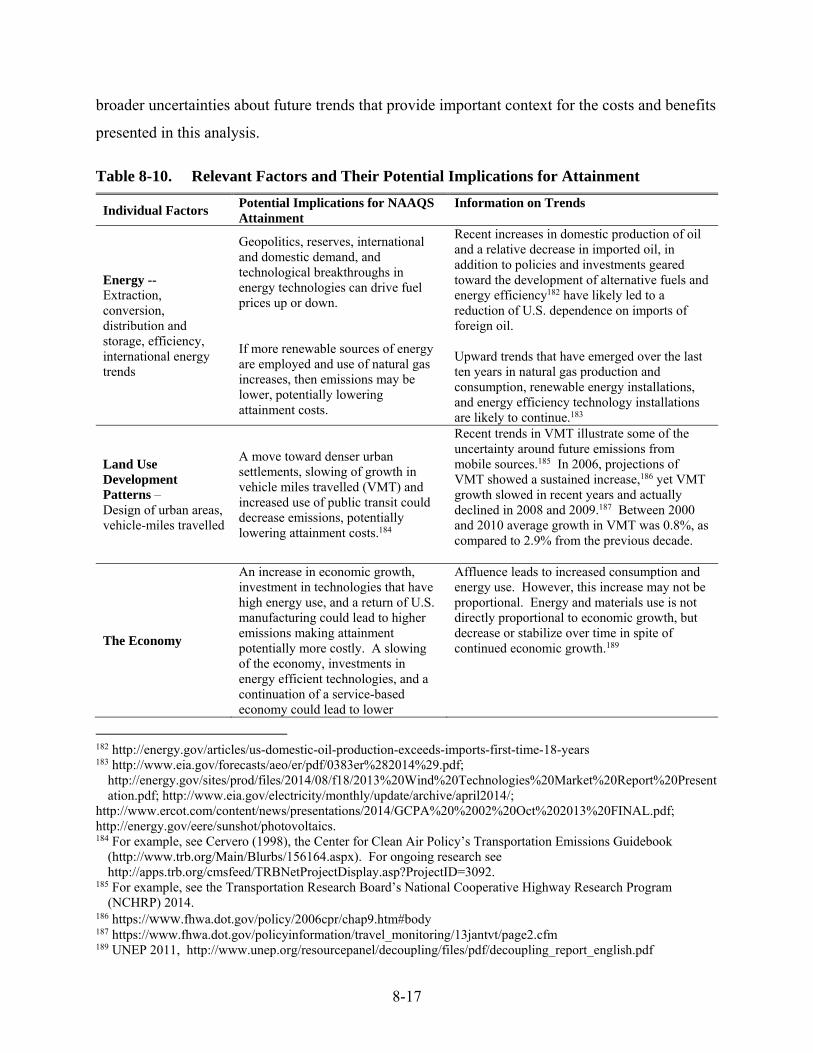
8-17
broader uncertainties about future trends that provide important context for the costs and benefits
presented in this analysis.
Table 8-10. Relevant Factors and Their Potential Implications for Attainment
Individual Factors Potential Implications for NAAQS Attainment
Information on Trends
Energy -- Extraction, conversion, distribution and storage, efficiency, international energy trends
Geopolitics, reserves, international and domestic demand, and technological breakthroughs in energy technologies can drive fuel prices up or down. If more renewable sources of energy are employed and use of natural gas increases, then emissions may be lower, potentially lowering attainment costs.
Recent increases in domestic production of oil and a relative decrease in imported oil, in addition to policies and investments geared toward the development of alternative fuels and energy efficiency182 have likely led to a reduction of U.S. dependence on imports of foreign oil. Upward trends that have emerged over the last ten years in natural gas production and consumption, renewable energy installations, and energy efficiency technology installations are likely to continue.183
Land Use Development Patterns – Design of urban areas, vehicle-miles travelled
A move toward denser urban settlements, slowing of growth in vehicle miles travelled (VMT) and increased use of public transit could decrease emissions, potentially lowering attainment costs.184
Recent trends in VMT illustrate some of the uncertainty around future emissions from mobile sources.185 In 2006, projections of VMT showed a sustained increase,186 yet VMT growth slowed in recent years and actually declined in 2008 and 2009.187 Between 2000 and 2010 average growth in VMT was 0.8%, as compared to 2.9% from the previous decade.
The Economy
An increase in economic growth, investment in technologies that have high energy use, and a return of U.S. manufacturing could lead to higher emissions making attainment potentially more costly. A slowing of the economy, investments in energy efficient technologies, and a continuation of a service-based economy could lead to lower
Affluence leads to increased consumption and energy use. However, this increase may not be proportional. Energy and materials use is not directly proportional to economic growth, but decrease or stabilize over time in spite of continued economic growth.189
182 http://energy.gov/articles/us-domestic-oil-production-exceeds-imports-first-time-18-years 183 http://www.eia.gov/forecasts/aeo/er/pdf/0383er%282014%29.pdf;
http://energy.gov/sites/prod/files/2014/08/f18/2013%20Wind%20Technologies%20Market%20Report%20Presentation.pdf; http://www.eia.gov/electricity/monthly/update/archive/april2014/;
http://www.ercot.com/content/news/presentations/2014/GCPA%20%2002%20Oct%202013%20FINAL.pdf; http://energy.gov/eere/sunshot/photovoltaics. 184 For example, see Cervero (1998), the Center for Clean Air Policy’s Transportation Emissions Guidebook
(http://www.trb.org/Main/Blurbs/156164.aspx). For ongoing research see http://apps.trb.org/cmsfeed/TRBNetProjectDisplay.asp?ProjectID=3092.
185 For example, see the Transportation Research Board’s National Cooperative Highway Research Program (NCHRP) 2014.
186 https://www.fhwa.dot.gov/policy/2006cpr/chap9.htm#body 187 https://www.fhwa.dot.gov/policyinformation/travel_monitoring/13jantvt/page2.cfm 189 UNEP 2011, http://www.unep.org/resourcepanel/decoupling/files/pdf/decoupling_report_english.pdf

8-18
Individual Factors Potential Implications for NAAQS Attainment
Information on Trends
emissions making attainment potentially less costly.188
Policiesa – Energy efficiency, energy security, direction of research and development, renewable energy
A move toward energy security and independence would mean an increased use of domestic energy sources. If this results in a fuel mix where emissions decrease, then attainment would likely be less costly. If not, attainment would likely be more costly. A move toward investments in fuel efficiency and low emissions fuels could decrease emissions and likely lower attainment costs.
State and local policies related to energy efficiency, cleaner energy, energy security190, as well as the direction of research and development of technology can have a direct or indirect effect on emissions. Policies that result in energy efficiency, renewable electric power, the use of cleaner fuels and conservation measures would likely result in decreased emissions and likely decrease attainment costs.191 Growth in energy demand has stayed well below growth in gross domestic product, likely as a result of technological advances, federal, state and local energy efficiency standards and policies, and other macroeconomic factors.192 U.S. productivity per energy expended relative to other countries suggests that additional efficiency gains are possible.193
Intensity, Location and Outcome of the Climate Change Signal
Strong climate signals that bring high temperatures could increase ozone, likely making attainment more costly.
Uncertainty exists regarding how the climate signal will interact with air quality, as well as with other factors. However, research demonstrates that in areas where there are both high levels of emissions and high temperatures, attaining an ozone standard will likely be much harder. The magnitudes of these impacts will depend on atmospheric chemical and physical processes, as well as anthropogenic activities that increase or decrease NOx and/or VOC emissions.194
Technological Change -- Including emissions reductions technologies and other technological developments
Innovation in production and emissions control technologies, learning that lower costs, and breakthroughs in battery/energy storage technologies for use with renewable energy could improve air quality, reducing emissions and likely lowering attainment costs.
Examples of emerging technologies include carbon capture and sequestration (CCS), battery technologies, emerging advanced biofuels, which could all have breakthroughs that could impact fuel use. Similarly, shifts in industrial production processes, such as a move from using primary metals to more recycling could impact energy use.195
a Policies refer to any policies or regulations that are not environmental regulations set by U.S. EPA, states, tribes, or local authorities.
188 For example, Bo (2011), and http://www.epa.gov/region1/airquality/nox.html for manufactures contributions to
NOX emissions. 190 For example, http://www2.epa.gov/laws-regulations/summary-energy-independence-and-security-act. 191 For example, see http://www.dsireusa.org/solar/solarpolicyguide/. 192 http://bipartisanpolicy.org/sites/default/files/BPC%20SEPI%20Energy%20Report%202013_0.pdf, p. 5. 193 http://bipartisanpolicy.org/sites/default/files/BPC%20SEPI%20Energy%20Report%202013_0.pdf, p. 69. 194 See Jacobs (2009). 195 http://www.eia.gov/todayinenergy/detail.cfm?id=16211
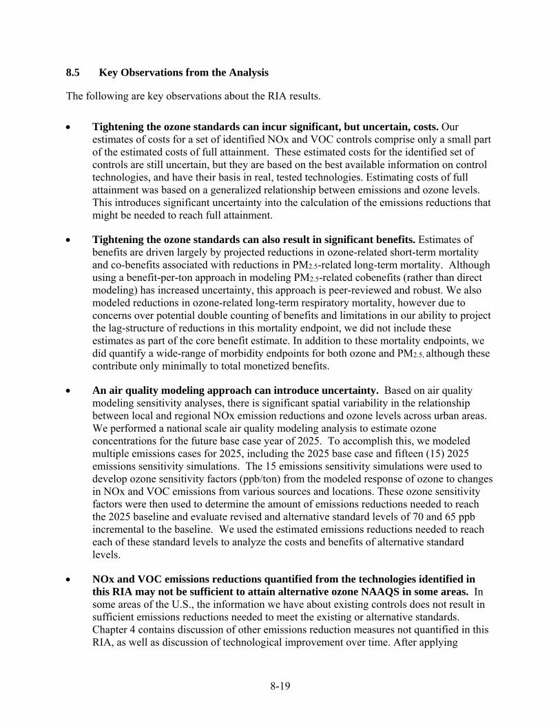
8-19
8.5 Key Observations from the Analysis
The following are key observations about the RIA results.
Tightening the ozone standards can incur significant, but uncertain, costs. Our estimates of costs for a set of identified NOx and VOC controls comprise only a small part of the estimated costs of full attainment. These estimated costs for the identified set of controls are still uncertain, but they are based on the best available information on control technologies, and have their basis in real, tested technologies. Estimating costs of full attainment was based on a generalized relationship between emissions and ozone levels. This introduces significant uncertainty into the calculation of the emissions reductions that might be needed to reach full attainment.
Tightening the ozone standards can also result in significant benefits. Estimates of benefits are driven largely by projected reductions in ozone-related short-term mortality and co-benefits associated with reductions in PM2.5-related long-term mortality. Although using a benefit-per-ton approach in modeling PM2.5-related cobenefits (rather than direct modeling) has increased uncertainty, this approach is peer-reviewed and robust. We also modeled reductions in ozone-related long-term respiratory mortality, however due to concerns over potential double counting of benefits and limitations in our ability to project the lag-structure of reductions in this mortality endpoint, we did not include these estimates as part of the core benefit estimate. In addition to these mortality endpoints, we did quantify a wide-range of morbidity endpoints for both ozone and PM2.5, although these contribute only minimally to total monetized benefits.
An air quality modeling approach can introduce uncertainty. Based on air quality modeling sensitivity analyses, there is significant spatial variability in the relationship between local and regional NOx emission reductions and ozone levels across urban areas. We performed a national scale air quality modeling analysis to estimate ozone concentrations for the future base case year of 2025. To accomplish this, we modeled multiple emissions cases for 2025, including the 2025 base case and fifteen (15) 2025 emissions sensitivity simulations. The 15 emissions sensitivity simulations were used to develop ozone sensitivity factors (ppb/ton) from the modeled response of ozone to changes in NOx and VOC emissions from various sources and locations. These ozone sensitivity factors were then used to determine the amount of emissions reductions needed to reach the 2025 baseline and evaluate revised and alternative standard levels of 70 and 65 ppb incremental to the baseline. We used the estimated emissions reductions needed to reach each of these standard levels to analyze the costs and benefits of alternative standard levels.
NOx and VOC emissions reductions quantified from the technologies identified in this RIA may not be sufficient to attain alternative ozone NAAQS in some areas. In some areas of the U.S., the information we have about existing controls does not result in sufficient emissions reductions needed to meet the existing or alternative standards. Chapter 4 contains discussion of other emissions reduction measures not quantified in this RIA, as well as discussion of technological improvement over time. After applying

8-20
existing rules and the illustrative identified controls across the nation (excluding California), in order to reach 70 ppb we were able to identify controls that reduce overall NOx emissions by 240,000 tons and VOC emissions by 20,000 tons. In order to reach 65 ppb we were able to identify controls that reduce overall NOx emissions by 560,000 tons and VOC emissions by 110,000 tons. After these reductions, in order to reach 70 ppb over 47,000 tons of NOx emissions remained, and in order to reach 65 ppb over 860,000 tons of NOx emissions remained.
California costs and benefits are highly uncertain. California faces large challenges in meeting any alternative standard, but their largest challenges may be in attaining the existing standard. Because our analysis suggested that all available controls would be exhausted in attempting to meet the current 75 ppb standard, all of the benefits and costs of lower standards in California are based on the application of unidentified controls. Both the benefits and the costs associated with the assumed NOx and VOC reductions in California are particularly uncertain.
Some EPA existing mobile source programs will help some areas reach attainment. These programs promise to continue to help areas reduce ozone concentrations beyond 2025. In California, continued implementation of mobile source rules, including the onroad and nonroad diesel rules and the locomotive and marine engines rule, are projected to reduce NOx emissions by an additional 14,000 tons and VOC emissions by an additional 6,300 tons between 2025 and 2030. These additional reductions will likely reduce the overall emissions reductions needed for attainment relative to what California might have needed to reduce from other sectors if attainment were to be required in 2025.
The economic impacts (i.e., social costs) of the cost of these modeled controls were not included in this analysis. Incorporating the economic impact of the unidentified portion of the emissions reductions was too uncertain to be included as part of these estimates. Therefore, we did not include the economic impacts of either the identified control costs or costs of unidentified controls.
Costs and benefits will depend on implementation timeframes. States will ultimately select the specific timelines for implementation as part of their State Implementation Plans. To the extent that states seek classification as extreme nonattainment areas, the timeline for implementation may be extended beyond 2025, meaning that the amount of emissions reductions that will be required in 2025 will be less, and costs and benefits in 2025 will be lower.
8.6 References
Cervero, R. (1998) The Transit Metropolis, A Global Inquiry. Island Press, Washington, D.C.
Jacob, D. J., & Winner, D. (2009). Effect of climate change on air quality. Atmospheric Environment, 43, 51-63.
Miller BG. Life table methods for quantitative impact assessments in chronic mortality. Journal of Epidemiology & Community Health, 2003; 57(3):200–206.
NCHRP (2014). The Effects of Socio-Demographics on Future Travel Demand, Transportation Research Board of the National Academies, Washington, D.C. Strategic Issues Facing Transportation, Report 750, Volume 6.

8-21
U.S. Environmental Protection Agency (U.S. EPA). 2008. Final Ozone NAAQS Regulatory Impact Analysis. Office of Air Quality Planning and Standards, Research Triangle Park, NC. Available at http://www.epa.gov/ttn/ecas/regdata/RIAs/452_R_08_003.pdf.
U.S. Environmental Protection Agency (U.S. EPA). 2010. Regulatory Impact Analysis (RIA) for the Proposed Reconsideration of the ozone National Ambient Air Quality Standards (NAAQS). Office of Air Quality Planning and Standards, Research Triangle Park, NC. January. Available at <http://www.epa.gov/ttn/ecas/regdata/RIAs/s1-supplemental_analysis_full.pdf>.
U.S. EPA. 2009. Integrated Science Assessment for Particulate Matter: Final. Research Triangle Park, NC: U.S. Environmental Protection Agency. (EPA document number EPA/600/R-08/139F).
U.S. EPA. 2013a. Integrated Science Assessment for Ozone and Related Photochemical Oxidants: Final. Research Triangle Park, NC: U.S. Environmental Protection Agency. (EPA document number EPA/600/R-10/076F).
U.S. EPA Science Advisory Board. Review of EPA’s DRAFT Health Benefits of the Second Section 812 Prospective Study of the Clean Air Act. Washington, DC, 2010.
9-1
CHAPTER 9: STATUTORY AND EXECUTIVE ORDER IMPACT ANALYSES
Overview
This section explains the statutory and executive orders applicable to EPA rules, and
discusses EPA’s actions taken pursuant to these orders.
9.1 Executive Order 12866: Regulatory Planning and Review
This action is an economically significant regulatory action that was submitted to the
Office of Management and Budget (OMB) for review. Any changes made in response to OMB
recommendations have been documented in the docket. This RIA estimates the costs and
monetized human health and welfare benefits of attaining two alternative ozone NAAQS
nationwide. Specifically, the RIA examines the alternatives of 65 ppb and 70 ppb. The RIA
contains illustrative analyses that consider a limited number of emissions control scenarios that
states and Regional Planning Organizations might implement to achieve these alternative ozone
NAAQS. However, the CAA and judicial decisions make clear that the economic and technical
feasibility of attaining ambient standards are not to be considered in setting or revising NAAQS,
although such factors may be considered in the development of state plans to implement the
standards. Accordingly, although an RIA has been prepared, the results of the RIA have not been
considered in issuing the revised NAAQS.
9.2 Paperwork Reduction Act
The information collection requirements for the revised NAAQS have been submitted for
approval to the Office of Management and Budget (OMB) under the Paperwork Reduction Act
(PRA). The information collection requirements are not enforceable until OMB approves them.
The Information Collection Request (ICR) document prepared by the EPA for these revisions
has been assigned EPA ICR #2313.04.
The information collected and reported under 40 CFR part 58 is needed to determine
compliance with the NAAQS, to characterize air quality and associated health and ecosystems
impacts, to develop emission control strategies, and to measure progress for the air pollution
program. We are extending the length of the required ozone monitoring season in 32 states and
the District of Columbia and the revised ozone monitoring seasons will become effective on
9-2
January 1, 2017. We are also revising the PAMS monitoring requirements to reduce the number
of required PAMS sites while improving spatial coverage, and requiring states in moderate or
above ozone non-attainment areas and the ozone transport region to develop an enhanced
monitoring plan as part of the PAMS requirements. Monitoring agencies will need to comply
with the PAMS requirements by June 1, 2019. In addition, we are revising the ozone FRM to
establish a new, additional technique for measuring ozone in the ambient air. It will be
incorporated into the existing ozone FRM, using the same calibration procedure in Appendix D
of 40 CFR part 50. We are also making changes to the procedures for testing performance
characteristics and determining comparability between candidate FEMs and reference methods.
For the purposes of ICR number 2313.04, the burden figures represent the burden
estimate based on the requirements contained in this rule. The burden estimates are for the 3-year
period from 2016 through 2018. The implementation of the PAMS changes will occur beyond
the time frame of this ICR with implementation occurring in 2019. The cost estimates for the
PAMS network (including revisions) will be captured in future routine updates to the Ambient
Air Quality Surveillance ICR that are required every 3 years by OMB. The addition of a new
FRM in 40 CFR part 50 and revisions to the ozone FEM procedures for testing performance
characteristics in 40 CFR part 53 does not add any additional information collection
requirements.
The ICR burden estimates are associated with the changes to the ozone seasons in the
revised NAAQS. This information collection is estimated to involve 158 respondents for a total
cost of approximately $24,597,485 (total capital, labor, and operation and maintenance) plus a
total burden of 339,930 hours for the support of all operational aspects of the entire ozone
monitoring network. The labor costs associated with these hours are $20,209,966. Also included
in the total are other costs of operations and maintenance of $2,254,334 and equipment and
contract costs of $2,133,185. The actual labor cost increase to expand the ozone monitoring
seasons is $2,064,707. In addition to the costs at the state, local, and tribal air quality
management agencies, there is a burden to EPA of 41,418 hours and $2,670,360. Burden is
defined at 5 CFR 1320.3(b). State, local, and tribal entities are eligible for state assistance grants
provided by the Federal government under the CAA which can be used for related activities. An
agency may not conduct or sponsor, and a person is not required to respond to, a collection of

9-3
information unless it displays a currently valid OMB control number. The OMB control numbers
for EPA’s regulations in 40 CFR are listed in 40 CFR part 9.
9.3 Regulatory Flexibility Act
This action will not have a significant economic impact on a substantial number of small
entities under the RFA. This action will not impose any requirements on small entities. Rather,
the rule establishes national standards for allowable concentrations of ozone in ambient air as
required by section 109 of the CAA. See also American Trucking Associations v. EPA, 175 F. 3d
at 1044-45 (NAAQS do not have significant impacts upon small entities because NAAQS
themselves impose no regulations upon small entities). Similarly, the revisions to 40 CFR part 58
address the requirements for states to collect information and report compliance with the
NAAQS and will not impose any requirements on small entities. Similarly, the addition of a new
FRM in 40 CFR part 50 and revisions to the FEM procedures for testing in 40 CFR part 53 will
not impose any requirements on small entities.
9.4 Unfunded Mandates Reform Act
This action does not contain any unfunded mandate as described in UMRA, 2 U. S. C.
1531 – 1538, and does not significantly or uniquely affect small governments. Furthermore, as
indicated previously, in setting a NAAQS the EPA cannot consider the economic or
technological feasibility of attaining ambient air quality standards, although such factors may be
considered to a degree in the development of state plans to implement the standards. See also
American Trucking Associations v. EPA, 175 F. 3d at 1043 (noting that because the EPA is
precluded from considering costs of implementation in establishing NAAQS, preparation of a
RIA pursuant to the UMRA would not furnish any information which the court could consider in
reviewing the NAAQS).
9.5 Executive Order 13132: Federalism
This action does not have federalism implications. It will not have substantial direct
effects on the states, on the relationship between the national government and the states, or on
the distribution of power and responsibilities among the various levels of government.

9-4
9.6 Executive Order 13175: Consultation and Coordination with Indian Tribal Governments
This action does not have tribal implications as specified in Executive Order 13175. It
does not have a substantial direct effect on one or more Indian Tribes as tribes are not obligated
to adopt or implement any NAAQS. In addition, tribes are not obligated to conduct ambient
monitoring for ozone or to adopt the ambient monitoring requirements of 40 CFR part 58. Thus,
Executive Order 13175 does not apply to this action.
The EPA specifically solicited comment on this rule from tribal officials. The EPA also
conducted outreach consistent with the EPA Policy on Consultation and Coordination with
Indian Tribes. Outreach to tribal environmental professionals was conducted through
participation in the Tribal Air call, which is sponsored by the National Tribal Air Association.
Consistent with the EPA Policy on Consultation and Coordination with Indian Tribes, the EPA
offered formal consultation to the tribes during the public comment period. Consultation was not
requested.
9.7 Executive Order 13045: Protection of Children from Environmental Health & Safety Risks
This action is subject to Executive Order 13045 because it is an economically significant
regulatory action as defined by Executive Order 12866, and the EPA believes that the
environmental health risk addressed by this action may have a disproportionate effect on
children. The rule will establish uniform NAAQS for ozone; these standards are designed to
protect public health with an adequate margin of safety, as required by CAA section 109.
However, the protection offered by these standards may be especially important for children
because children, especially children with asthma, along with other at-risk populations196 such
as all people with lung disease and people active outdoors, are at increased risk for health effects
associated with exposure to ozone in ambient air. Because children are considered an at-risk
lifestage, we have carefully evaluated the environmental health effects of exposure to ozone
pollution among children. Discussions of the results of the evaluation of the scientific evidence,
196 As used here and similarly throughout this document, the term population refers to people having a quality or characteristic in common, including a specific pre-existing illness or a specific age or lifestage.

9-5
policy considerations, and the exposure and risk assessments pertaining to children are contained
in sections II.B and II.C of the preamble.
9.8 Executive Order 13211: Actions that Significantly Affect Energy Supply, Distribution, or Use
This action is not a “significant energy action” because it is not likely to have a
significant adverse effect on the supply, distribution, or use of energy. The purpose of the rule is
to establish a revised NAAQS for ozone, establish an additional FRM, revise FEM procedures
for testing, and revises air quality surveillance requirements. The rule does not prescribe specific
pollution control strategies by which these ambient standards and monitoring revisions will be
met. Such strategies will be developed by states on a case-by-case basis, and the EPA cannot
predict whether the control options selected by states will include regulations on energy
suppliers, distributors, or users. Thus, the EPA concludes that this rule is not likely to have any
adverse energy effects and does not constitute a significant energy action as defined in Executive
Order 13211.
Application of the modeled illustrative control strategy containing identified controls for
power plants, shown in Chapter 4, means that 4 percent of the total projected coal-fired EGU
capacity nationwide in 2025 could be affected by controls for the revised standard level of 70
ppb. Similarly, 13 percent of total projected coal-fired EGU capacity in 2025 could be affected
by controls for the alternative standard of 65 ppb. In addition, some fuel switching might occur
that could alter these percentages, although we are not able to estimate the effect on energy
impacts from fuel switching. In addition, we are not able to estimate energy impacts resulting
from application of controls to non-EGUs or mobile sources. It is important to note that the
estimates presented above are just one illustrative strategy and states may choose to apply
controls to sources other than EGUs for the purpose of attaining a more stringent standard.
9.9 National Technology Transfer and Advancement Act
This rulemaking involves environmental monitoring and measurement. Consistent with
the Agency’s Performance Based Measurement System (PBMS), the EPA is not requiring the
use of specific, prescribed analytical methods. Rather, the Agency is allowing the use of any
method that meets the prescribed performance criteria. Ambient air concentrations of ozone are

9-6
currently measured by the Federal reference method (FRM) in 40 CFR part 50, Appendix D
(Measurement Principle and Calibration Procedure for the Measurement of Ozone in the
Atmosphere) or by Federal equivalent methods (FEM) that meet the requirements of 40 CFR part
53. Procedures are available in part 53 that allow for the approval of an FEM for ozone that is
similar to the FRM. Any method that meets the performance criteria for a candidate equivalent
method may be approved for use as an FEM. This approach is consistent with EPA’s PBMS. The
PBMS approach is intended to be more flexible and cost-effective for the regulated community;
it is also intended to encourage innovation in analytical technology and improved data quality.
The EPA is not precluding the use of any method, whether it constitutes a voluntary consensus
standard or not, as long as it meets the specified performance criteria.
9.10 Executive Order 12898: Federal Actions to Address Environmental Justice in Minority Populations and Low-Income Populations
The EPA believes that this action will not have disproportionately high and adverse
human health or environmental effects on minority populations, low-income populations or
indigenous peoples. The action described in this notice is to strengthen the NAAQS for ozone.
The primary NAAQS are established at a level that is requisite to protect public health,
including the health of sensitive or at-risk groups, with an adequate margin of safety. The
NAAQS decisions are based on an explicit and comprehensive assessment of the current
scientific evidence and associated exposure/risk analyses. More specifically, EPA expressly
considers the available information regarding health effects among at-risk populations, including
that available for low-income populations and minority populations, in decisions on NAAQS.
Where low-income populations or minority populations are among the at-risk populations, the
decision on the standard is based on providing protection for these and other at-risk populations
and lifestages. Where such populations are not identified as at-risk populations, a NAAQS that
is established to provide protection to the at-risk populations would also be expected to provide
protection to all other populations, including low-income populations and minority populations.
The Integrated Science Assessment, the Health Risk and Exposure Assessment, and the
Policy Assessment for this review, which include identification of populations at risk from ozone
health effects, are available in the docket EPA-HQ-OAR-2008-0699. The information on at-risk
9-7
populations for this NAAQS review is summarized and considered in the rule preamble (see
section II.A). The final rule increases the level of environmental protection for all affected
populations without having any disproportionately high and adverse human health or
environmental effects on any population, including any minority populations, low-income
populations or indigenous peoples. The rule establishes uniform national standards for ozone in
ambient air that, in the Administrator’s judgment, protect public health, including the health of
sensitive groups, with an adequate margin of safety.
Although it has a separate docket and is not part of the rulemaking record for this action,
EPA has prepared a RIA of this decision. As part of the RIA, a demographic analysis was
conducted. While, as noted in the RIA, the demographic analysis is not a full quantitative, site-
specific exposure and risk assessment, that analysis examined demographic characteristics of
persons living in areas with poor air quality relative to the revised standard. Specifically,
Appendix 9A describes the proximity and socio-demographic analysis. The analysis found that
in areas with poor air quality relative to the revised standard,197 the representation of minority
populations was slightly greater than in the U.S. as a whole. Because the air quality in these areas
does not currently meet the revised standard, populations in these areas would be expected to
benefit from implementation of the strengthened standard, and, thus, would be more affected by
strategies to attain the revised standard. The analysis, which evaluates the potential implications
for minority populations and low-income populations of future air pollution control actions that
state and local agencies may consider in implementing the revised ozone NAAQS described in
the decision notice, is discussed in Appendix 9A. The RIA is available on the Web, through the
EPA’s Technology Transfer Network website at
http://www.epa.gov/ttn/naaqs/standards/ozone/s_o3_index.html and in the RIA docket (EPA-
HQ-OAR-2013-0169). As noted above, although an RIA has been prepared, the results of the
RIA have not been considered in issuing this final rule.
197 This refers to monitored areas with ozone design values above the revised and alternative standards.

9-8
9.11 Congressional Review Act (CRA)
This action is subject to the CRA, and the EPA will submit a rule report to each House of
the Congress and to the Comptroller General of the United States. This action is a “major rule”
as defined by 5 U.S.C. 804(2).
9A-1
APPENDIX 9A: SOCIO-DEMOGRAPHIC CHARACTERISTICS OF POPULATIONS IN CORE BASED STATISTICAL AREAS WITH OZONE MONITORS EXCEEDING REVISED AND ALTERNATIVE OZONE STANDARDS
Overview
The Environmental Protection Agency’s (EPA) Office of Air Quality Planning and
Standards (OAQPS) has conducted a limited analysis of population demographics in some areas
that may be affected by the revisions to the National Ambient Air Quality Standards (NAAQS)
for ozone. This appendix describes a limited screening-level analysis of the socio-demographic
characteristics of populations living in areas with an ozone monitor with a current (2012-2014)
design value exceeding the revised and alternative ozone standard levels of 70 and 65 parts per
billion (ppb). This analysis does not include a quantitative assessment of exposure and/or risk for
populations of potential interest from an environmental justice (EJ) perspective, and therefore it
cannot be used to draw any conclusions regarding potential disparities in exposure or risk across
populations of interest from an EJ perspective. This appendix describes the technical approach
used in the analysis, discusses uncertainties and limitations associated with the analysis, and
presents results.
The EPA Administrator is revising the NAAQS for ozone from the current level of 75
ppb to a level of 70 ppb. The revisions will establish uniform national standards for ozone in
ambient air and improve public health protection for at-risk groups, especially children. The
Agency has elected to conduct a limited analysis of key socio-demographic characteristics of
populations living in areas with poor ozone air quality, defined for this analysis as any Core
Based Statistical Area (CBSA) with at least one county having an ozone monitor with a current
(2012-2014) design value exceeding the revised and alternative ozone standard levels (70 and 65
ppb), including individual counties not included in a CBSA with a design value exceeding the
revised and alternative standards. These areas are called “study areas” for the purposes of this
analysis.
9A.1 Design of Analysis
To gain a better understanding of the populations within the study areas, the EPA
conducted an analysis at the county level for this ozone NAAQS review. The study areas for
these analyses were defined as all counties contained within any CBSA with at least one monitor

9A-2
with a current (2012-2014) design value above the revised and alternative standard levels (70 and
65 ppb) as well as counties not in a CBSA with a current (2012-2014) design value above the
revised and alternative standard levels (70 and 65 ppb). The study areas were designed to capture
population and communities with poor ozone air quality, and areas most likely to benefit from
improved air quality following the implementation of the revised ozone NAAQS.
For the revised standard levels of 70 ppb, 511 counties were analyzed in 143 areas
exceeding the standard levels, including 495 counties in 127 CBSAs and 16 counties outside
CBSAs. For the alternative standard levels of 65 ppb, 891 counties were analyzed in 294 areas
exceeding the standard level, including 847 counties in 250 CBSAs and 44 counties outside
CBSAs. The population identified within these study areas made up about 52% of the U.S.
population for the revised standard levels and about 69% of the U.S. population for the
alternative standard levels.
Demographic data from the study areas identified for the revised and alternative standard
levels were aggregated nationally for comparison with the U.S. population demographics. The
demographic data used in this analysis include race, ethnicity, age, income, and education
variables. Details on these demographic groups are provided in the following section (9A.1.1).
The aggregated demographic values across the study areas are compared to the national data in
Table 9A-2 of Section 9A-3.
This analysis identifies, on a limited basis, the populations that are most likely to
experience reductions in ozone concentrations as a result of actions taken to meet the revised
standard levels, and thus are expected to benefit most from this regulation. This analysis does not
identify the demographic characteristics of the most highly affected individuals or communities
nor does it quantify the level of risk faced by those individuals or communities. To the extent
that any populations are disproportionately impacted by ozone levels because they reside in a
study area, that population will also experience increased environmental and health benefits from
meeting the revised standard levels.

9A-3
9A.1.1 Demographic Variables Included in Analysis
This analysis includes race, ethnicity, and age data derived from the 2010 Census SF1
dataset198 and income and education data from the Census Bureau’s 2006-2010 American
Community Survey (ACS) 5-Year Estimates.199 This data is summarized in Table 9A-1.
Table 9A-1. Census Derived Demographic Data
Race, Ethnicity, and Age Data (Census 2010 block-level SF1 data)*
Parameter Definition
Population Total population
White Number of whites (may include Hispanics)
African American Number of African Americans (may include Hispanics)
Native American Number of Native Americas (may include Hispanics)
Other and multiracial Number of other race and multiracial (may include Hispanics)
Minority Total Population less White Population
Hispanic Number of Hispanics
Age 0 to 4 Number of people age 0 to 4
Age 0 to 17 Number of people age 0 to 17
Age 65 and up Number of people age 65 and up
Economic and Education Date (2006-2010 ACS)*
Parameter Definition
Education level Number of adults age 25 years and up without a high school diploma
Low Income Number of people living in households with income below twice the
poverty line
Linguistic Isolation Number of people linguistically isolated
*Census 2010 does not currently report this data for the Virgin Islands, Guam, American Samoa, and the Northern Marianas; Census 2000 data are used for these areas.
As noted above, the EPA uses population data collected by the 2010 Census. All data is
stored at the block level. For those indicators available from the Census at the block group, but
not block level, the EPA assigns a block the same percentage as the block group of which it is a
198 2010 Census Summary File 1 Delivered via FTP, http://www2.census.gov/census_2010/04-Summary_File_1/ 199 U.S. Census Bureau 2006-2010 American Community Survey 5-Year Estimates, http://www.census.gov/acs/www/data_documentation/2010_release/

9A-4
part. For example, a block is assigned the same percentage of people living below the national
poverty line as the block group in which it is contained. Nationally, a census block contains
about 50 people on average; and a block group contains about 26 blocks on average, or about
1,350 people. For comparison, a census tract is larger than a block group, with each tract
containing an average of 3 block groups, or about 4,300 people. For this analysis, the data was
aggregated to the county level.
Data on race, ethnicity and age for all census blocks in the country except for the Virgin
Islands, Guam, American Samoa, and the Northern Marianas were obtained from the 2010
Census SF1 dataset. This dataset provides the population for each census block among different
racial and ethnic classifications, including: White, African American or Black, Hispanic or
Latino, American Indian or Native Alaskan, Asian, Native Hawaiian or other South Pacific
Islander, other race, and two or more races. Data on age distributions in the U.S. and Puerto Rico
were obtained at the census block level from the 2010 Census of Population and Housing
Summary File 1 (SF1) short form. SF1 contains the information compiled from the questions
asked of all people about every housing unit. Data on poverty status, education level, and
linguistic isolation in the U.S. and Puerto Rico were obtained at the block group level from the
Census Bureau’s 2006-2010 ACS.
9A.2 Considerations in Evaluating and Interpreting Results
This analysis characterizes the demographic attributes of populations located in areas
defined by a county or a CBSA containing a county with a monitored 2012-2014 design value
greater than the revised standard levels of 70 ppb, or the alternative standard levels of 65 ppb.
Therefore, the results of this analysis can only be used to inform whether there are differences in
the composition of populations residing within these areas relative to the nation as a whole. As
noted earlier, the purpose of the analysis is to determine whether populations of interest from an
EJ perspective have a higher representation in areas that exceed the revised and alternative ozone
standard levels, and thus may be more affected by implementation of the revised standards. This
analysis does not include a quantitative assessment of exposure or risk for specific populations of
potential interest from an EJ-perspective, and therefore it cannot be used to draw any conclusions
regarding potential disparities in exposure or risk across populations of interest from an EJ
perspective. Nor can it be used to draw conclusions about any disparities in the health and
environmental benefits that could result from implementation of the revised ozone standards.
9A-5
The analysis simply represents a national depiction of the baseline characteristics of populations
residing in areas with measured ozone air quality above the revised and alternative standard
levels.
In order to clearly identify disparities in risk between populations of interest, we would
need to conduct rigorous site-specific population-level exposure and risk assessments that take
into account short-term mobility (daily patterns of travel linked for example to school or work)
or long-term mobility (families moving into or out of specific block groups). EPA does not have
the ability to conduct such a rigorous technical analysis at this time.
9A.3 Presentation of Results
This section presents a summary of the demographics of populations in areas with 2012-
2014 design values greater than the revised and alternative ozone standard levels. The results are
provided in Table 9A-2. As a whole, the demographic distributions within the study areas
estimated for the revised and alternative standard levels (i.e., 70 ppb and 65 ppb) are similar to
the national averages. The largest difference is only 5%, between the national and study area
percentages for the Minority demographic group. Overall, these qualitative results support the
determination that the revised rule will tend to benefit geographic areas that have a higher
proportion of minority residents than the national average.

9A-6
Table 9A-2 Summary of Population Totals and Demographic Categories for Areas of Interest and National Perspective
Demographic Summary Population White African
American Native
American Other or
Multiracial Minority Hispanic Area Total - 70 ppb 163,900,459 109,711,305 23,448,540 1,196,130 29,544,484 54,189,154 33,651,929 % of Area Total - 70 ppb 67% 14% 1% 18% 33% 21% Area Total - 65 ppb 216,932,408 150,701,600 29,091,602 1,699,450 35,439,756 66,230,808 39,746,762 % of Area Total - 65 ppb 69% 13% 1% 16% 31% 18% National Total 312,861,256 226,405,205 39,475,216 2,952,087 44,028,748 86,456,051 54,181,245 % of National Total 72% 13% 1% 14% 28% 17%
Demographic Summary Population Age 0 to 4 Age 0 to 17 Age 65+
No High School
Diploma Low IncomeLinguistically
Isolated Area Total - 70 ppb 163,900,459 11,028,428 40,546,150 19,510,553 15,960,333 49,392,881 11,150,433 % of Area Total - 70 ppb 7% 25% 12% 10% 30% 7% Area Total - 65 ppb 216,932,408 14,387,223 52,913,376 26,596,432 20,469,632 65,336,396 13,050,626 % of Area Total - 65 ppb 7% 24% 12% 9% 30% 6% National Total 312,861,256 20,465,065 75,217,176 40,830,262 30,952,789 101,429,436 19,196,507 % of National Total 7% 24% 13% 10% 32% 6%

United States Environmental Protection Agency
Office of Air Quality Planning and Standards Health and Environmental Impacts Division
Research Triangle Park, NC
Publication No. EPA-452/R-15-007
September 2015