Universidad Politecnica de MadridFacultad de Informatica

Departamento de Inteligencia Artificial

Regularized Model Learning inEDAs for Continuous and

Multi-Objective Optimization

A Thesissubmitted to the Department of Artificial Intelligence at the School of

Computer Science of the Technical University of Madrid, as partialfulfillment of the requirements for the degree of Doctor of Philosophy

By

Hossein Karshenas

Supervisors

Pedro Larranaga and Concha Bielza

2013

ii

I want to dedicate this thesis to my family, who has always been a sourceof love, inspiration and encouragement in my life.

And, in loving memory of my dear grandmother.

iii

iv

Acknowledgements

The work presented in this thesis would have not been possible without all the helpand assistance I received from many individuals. First of all, I would like to thankmy supervisors, Pedro Larranaga and Concha Bielza, for their guidance, support andpatience. I have learnt a lot from them during this period of time, and our meetings andtalks gave me many new inspirations and motivations for completing this work.

I am very grateful to Roberto Santana who has been like a third supervisor to me.Our meetings, discussions and chats helped me to obtain a better understanding of EDAsand gave me many new ideas for advancing in my research. Thank you Roberto for yourhelp.

I also want to thank Fernando Lobo for receiving me as a visitor in his laboratory inthe University of Algarve at Faro, Portugal. I enjoyed very much the calm and friendlyworking environment with all the people at the laboratory, especially Mosab Bazarganiand Hossein Moeinzadeh, who helped me a lot during my stay there.

I like to mention the Consolider Ingenio 2010-CSD-2007-00018 and TIN2010-20900-C04-04 projects, and the financial grant GI111015026 from the Technical University ofMadrid, which supported me during this period of time while I was working as a PhDstudent.

At last but not least, I am grateful to all my friends and colleagues at the Com-putational Intelligence Group, Ruben Armananzas, Diego Vidaurre, Hanen Borchani,Pedro Luis Lopez-Cruz, Alfonso Ibanez, Luis Guerra, Bojan Mihaljevic and Laura Anton-Sanchez, for all of their supports and assistances and for providing an excellent workingenvironment. Thanks to all of you.

v

vi

Abstract

Probabilistic modeling is the defining characteristic of estimation of distribution algo-rithms (EDAs) which determines their behavior and performance in optimization. Regu-larization is a well-known statistical technique used for obtaining an improved model byreducing the generalization error of estimation, especially in high-dimensional problems.`1-regularization is a type of this technique with the appealing variable selection propertywhich results in sparse model estimations.

In this thesis, we study the use of regularization techniques for model learning inEDAs. Several methods for regularized model estimation in continuous domains basedon a Gaussian distribution assumption are presented, and analyzed from different aspectswhen used for optimization in a high-dimensional setting, where the population size ofEDA has a logarithmic scale with respect to the number of variables. The optimizationresults obtained for a number of continuous problems with an increasing number of vari-ables show that the proposed EDA based on regularized model estimation performs a morerobust optimization, and is able to achieve significantly better results for larger dimensionsthan other Gaussian-based EDAs. We also propose a method for learning a marginallyfactorized Gaussian Markov random field model using regularization techniques and aclustering algorithm. The experimental results show notable optimization performance oncontinuous additively decomposable problems when using this model estimation method.

Our study also covers multi-objective optimization and we propose joint probabilisticmodeling of variables and objectives in EDAs based on Bayesian networks, specificallymodels inspired from multi-dimensional Bayesian network classifiers. It is shown thatwith this approach to modeling, two new types of relationships are encoded in the esti-mated models in addition to the variable relationships captured in other EDAs: objective-variable and objective-objective relationships. An extensive experimental study shows theeffectiveness of this approach for multi- and many-objective optimization. With the pro-posed joint variable-objective modeling, in addition to the Pareto set approximation, thealgorithm is also able to obtain an estimation of the multi-objective problem structure.

Finally, the study of multi-objective optimization based on joint probabilistic model-ing is extended to noisy domains, where the noise in objective values is represented byintervals. A new version of the Pareto dominance relation for ordering the solutions inthese problems, namely α-degree Pareto dominance, is introduced and its properties areanalyzed. We show that the ranking methods based on this dominance relation can re-sult in competitive performance of EDAs with respect to the quality of the approximatedPareto sets. This dominance relation is then used together with a method for joint prob-abilistic modeling based on `1-regularization for multi-objective feature subset selection inclassification, where six different measures of accuracy are considered as objectives withinterval values. The individual assessment of the proposed joint probabilistic modeling

vii

and solution ranking methods on datasets with small-medium dimensionality, when usingtwo different Bayesian classifiers, shows that comparable or better Pareto sets of featuresubsets are approximated in comparison to standard methods.

viii

Resumen

La modelizacion probabilista es la caracterıstica definitoria de los algoritmos de estimacionde distribuciones (EDAs, en ingles) que determina su comportamiento y rendimiento enproblemas de optimizacion. La regularizacion es una tecnica estadıstica bien conocidautilizada para obtener mejores modelos al reducir el error de generalizacion de la esti-macion, especialmente en problemas de alta dimensionalidad. La regularizacion `1 tienela atractiva propiedad de seleccionar variables, lo que permite estimaciones de modelosdispersos.

En esta tesis, estudiamos el uso de tecnicas de regularizacion para el aprendizaje demodelos en EDAs. Se presentan y analizan dos aproximaciones para la estimacion delmodelo regularizado en dominios continuos basado en la asuncion de distribucion Gaus-siana desde diferentes aspectos en situaciones de alta dimensionalidad, donde el tamanode la poblacion del EDA es logarıtmico en el numero de variables. Los resultados deoptimizacion obtenidos para algunos problemas continuos, con un numero creciente devariables, muestran que el EDA propuesto, basado en la estimacion del modelo regular-izado, realiza una optimizacion mas robusta y es capaz de lograr resultados significativa-mente mejores para dimensiones mas grandes en comparacion con otros EDAs basados enla asuncion de distribucion Gaussiana. Tambien proponemos un metodo para aprenderun modelo de campo aleatorio de Markov Gaussiano que esta marginalmente factorizadoutilizando tecnicas de regularizacion y un algoritmo de clustering. Los resultados ex-perimentales muestran un rendimiento notable en optimizacion de problemas continuosaditivamente descomponibles cuando se utiliza este metodo de estimacion del modelo.

Nuestro estudio tambien cubre optimizacion multi-objetivo y proponemos una mod-elizacion probabilıstica conjunta de variables y objetivos en EDAs basada en redes Bayesi-anas, especıficamente redes Bayesianas multidimensionales. Se demuestra que con esteenfoque de modelizacion, en los modelos estimados se codifican dos nuevos tipos de rela-ciones ademas de las relaciones de variables capturadas en otros EDAs: relaciones deobjetivo-variable y de objetivo-objetivo. Un amplio estudio experimental muestra la efec-tividad de este enfoque para optimizacion multi-objetivo y para muchos objetivos. Con lamodelizacion propuesta, conjunta para variables y objetivos, ademas de la aproximaciondel conjunto de Pareto, el algoritmo es tambien capaz de obtener una estimacion de laestructura del problema multi-objetivo.

Por ultimo, el estudio de optimizacion multi-objetivo basado en modelizacion prob-abilıstica conjunta se extiende a dominios con ruido, donde el ruido en los valores delos objetivos se representa por intervalos. Se introduce una nueva version de la relacionde dominancia de Pareto para ordenar las soluciones en estos problemas, denominadadominancia de Pareto de grado α, y se analizan sus propiedades. Mostramos que losmetodos de ordenacion basados en esta relacion de dominancia pueden resultar en EDAs

ix

con un rendimiento competitivo con respecto a la calidad de la aproximacion del con-junto dePareto. Esta relacion de dominancia se utiliza despues junto con un metodode modelizacion probabilıstica conjunta basado en regularizacion `1 para seleccion multi-objetivo de subconjuntos de caracterısticas en clasificacion, donde se consideran seis me-didas diferentes de precision como los objetivos con valores de intervalo. La evaluacionindividual de estas dos propuestas de modelacion probabilıstica conjunta y los metodosde ordenacion en conjuntos de datos de pequena-mediana dimensionalidad, cuando seutilizan dos clasificadores Bayesianos diferentes, demuestra que se aproximan conjuntosde Pareto de subconjuntos de caracterısticas que comparables o mejores que con metodosestandar.

x

Contents

Preface xv

I Introduction 1

1 Probabilistic Graphical Models 3

1.1 Introduction . . . . . . . . . . . . . . . . . . . . . . . . . . . . . . . . . . 3

1.2 Probability-Related Notations . . . . . . . . . . . . . . . . . . . . . . . . 3

1.3 Bayesian Networks . . . . . . . . . . . . . . . . . . . . . . . . . . . . . . 4

1.3.1 Bayesian Network Parameterization . . . . . . . . . . . . . . . . . 5

1.3.2 Inference in Bayesian Networks . . . . . . . . . . . . . . . . . . . 8

1.3.3 Learning Bayesian Networks . . . . . . . . . . . . . . . . . . . . . 9

1.3.4 Bayesian Networks in Machine Learning . . . . . . . . . . . . . . 12

1.4 Markov Networks . . . . . . . . . . . . . . . . . . . . . . . . . . . . . . . 14

1.4.1 Multivariate Gaussian Distribution . . . . . . . . . . . . . . . . . 15

1.4.2 Gaussian Markov Random Fields . . . . . . . . . . . . . . . . . . 16

1.4.3 Learning and Sampling Gaussian Markov Networks . . . . . . . . 17

1.5 Conclusions . . . . . . . . . . . . . . . . . . . . . . . . . . . . . . . . . . 18

2 Evolutionary Optimization with Probabilistic Modeling 19

2.1 Introduction . . . . . . . . . . . . . . . . . . . . . . . . . . . . . . . . . . 19

2.2 Evolutionary Algorithms . . . . . . . . . . . . . . . . . . . . . . . . . . . 19

2.2.1 Genetic Algorithms . . . . . . . . . . . . . . . . . . . . . . . . . . 20

2.2.2 Evolutionary Strategy . . . . . . . . . . . . . . . . . . . . . . . . 20

2.2.3 Genetic Programming . . . . . . . . . . . . . . . . . . . . . . . . 21

2.2.4 Complementary Methods . . . . . . . . . . . . . . . . . . . . . . . 21

2.3 Estimation of Distribution Algorithms . . . . . . . . . . . . . . . . . . . 22

2.3.1 Discrete EDAs . . . . . . . . . . . . . . . . . . . . . . . . . . . . 24

2.3.2 Continuous EDAs . . . . . . . . . . . . . . . . . . . . . . . . . . . 27

2.3.3 Discrete-Continuous EDAs . . . . . . . . . . . . . . . . . . . . . . 29

2.3.4 Discussion . . . . . . . . . . . . . . . . . . . . . . . . . . . . . . . 29

2.3.5 Model-Based Genetic Programming . . . . . . . . . . . . . . . . . 31

2.4 Conclusions . . . . . . . . . . . . . . . . . . . . . . . . . . . . . . . . . . 32

xi

3 Evolutionary Algorithms in Bayesian Network Inference and Learning 333.1 Introduction . . . . . . . . . . . . . . . . . . . . . . . . . . . . . . . . . . 333.2 Triangulation of the Moral Graph . . . . . . . . . . . . . . . . . . . . . . 333.3 Total and Partial Abductive Inference . . . . . . . . . . . . . . . . . . . . 353.4 Structure Search . . . . . . . . . . . . . . . . . . . . . . . . . . . . . . . 36

3.4.1 DAG Space . . . . . . . . . . . . . . . . . . . . . . . . . . . . . . 373.4.2 Equivalence Class Space . . . . . . . . . . . . . . . . . . . . . . . 383.4.3 Ordering Space . . . . . . . . . . . . . . . . . . . . . . . . . . . . 39

3.5 Learning Dynamic Bayesian Networks . . . . . . . . . . . . . . . . . . . . 403.6 Learning Bayesian Network Classifiers . . . . . . . . . . . . . . . . . . . 413.7 Conclusions . . . . . . . . . . . . . . . . . . . . . . . . . . . . . . . . . . 42

II Regularization-Based Continuous Optimization 45

4 Introduction to Regularization 474.1 Introduction . . . . . . . . . . . . . . . . . . . . . . . . . . . . . . . . . . 474.2 Regularized Regression Models . . . . . . . . . . . . . . . . . . . . . . . . 484.3 Regularized Graphical Models . . . . . . . . . . . . . . . . . . . . . . . . 504.4 Conclusions . . . . . . . . . . . . . . . . . . . . . . . . . . . . . . . . . . 53

5 Regularized Model Learning in EDAs 555.1 Introduction . . . . . . . . . . . . . . . . . . . . . . . . . . . . . . . . . . 555.2 Approaches to Regularized Model Learning . . . . . . . . . . . . . . . . . 565.3 Analyzing Regularized Model Learning Methods . . . . . . . . . . . . . . 57

5.3.1 True Structure Recovery . . . . . . . . . . . . . . . . . . . . . . . 585.3.2 Time Complexity . . . . . . . . . . . . . . . . . . . . . . . . . . . 615.3.3 Likelihood Function . . . . . . . . . . . . . . . . . . . . . . . . . . 645.3.4 Regularization Parameter in Graphical LASSO Method . . . . . . 65

5.4 Conclusions . . . . . . . . . . . . . . . . . . . . . . . . . . . . . . . . . . 66

6 Regularization-Based EDA in Continuous Optimization 696.1 Introduction . . . . . . . . . . . . . . . . . . . . . . . . . . . . . . . . . . 696.2 RegEDA: Regularization-based EDA . . . . . . . . . . . . . . . . . . . . 696.3 Experiments . . . . . . . . . . . . . . . . . . . . . . . . . . . . . . . . . . 70

6.3.1 Optimization Functions . . . . . . . . . . . . . . . . . . . . . . . 706.3.2 Experimental Design . . . . . . . . . . . . . . . . . . . . . . . . . 726.3.3 Results . . . . . . . . . . . . . . . . . . . . . . . . . . . . . . . . . 736.3.4 Discussion . . . . . . . . . . . . . . . . . . . . . . . . . . . . . . . 80

6.4 Conclusions . . . . . . . . . . . . . . . . . . . . . . . . . . . . . . . . . . 82

7 Regularization in Factorized Gaussian Markov Random Field-BasedEDA 837.1 Introduction . . . . . . . . . . . . . . . . . . . . . . . . . . . . . . . . . . 837.2 GMRF-Based EDA with Marginal Factorization . . . . . . . . . . . . . . 83

7.2.1 A Hybrid Approach to Learn GMRF . . . . . . . . . . . . . . . . 847.2.2 Sampling Undirected Graphical Models for Continuous Problems 86

xii

7.3 Related Work . . . . . . . . . . . . . . . . . . . . . . . . . . . . . . . . . 867.4 Experiments . . . . . . . . . . . . . . . . . . . . . . . . . . . . . . . . . . 87

7.4.1 Benchmark Functions . . . . . . . . . . . . . . . . . . . . . . . . . 877.4.2 Results . . . . . . . . . . . . . . . . . . . . . . . . . . . . . . . . . 897.4.3 Influence of the Regularization Parameter . . . . . . . . . . . . . 90

7.5 Conclusions . . . . . . . . . . . . . . . . . . . . . . . . . . . . . . . . . . 91

III Multi-objective Optimization 93

8 Evolutionary Multi-Objective Optimization with Probabilistic Model-ing 958.1 Introduction . . . . . . . . . . . . . . . . . . . . . . . . . . . . . . . . . . 958.2 EDAs in Multi-Objective Optimization . . . . . . . . . . . . . . . . . . . 96

8.2.1 A Survey of Multi-Objective EDAs . . . . . . . . . . . . . . . . . 978.3 Conclusions . . . . . . . . . . . . . . . . . . . . . . . . . . . . . . . . . . 99

9 Evolutionary Multi-Objective Optimization with Joint Probabilistic Mod-eling 1019.1 Introduction . . . . . . . . . . . . . . . . . . . . . . . . . . . . . . . . . . 1019.2 Joint Probabilistic Modeling in Multi-Objective EDAs . . . . . . . . . . . 102

9.2.1 Discussion . . . . . . . . . . . . . . . . . . . . . . . . . . . . . . . 1039.3 JGBN-EDA for Continuous Multi-Objective Optimization . . . . . . . . 104

9.3.1 Solution Ranking and Selection . . . . . . . . . . . . . . . . . . . 1049.3.2 Joint Model Learning and Sampling . . . . . . . . . . . . . . . . . 105

9.4 Experiments . . . . . . . . . . . . . . . . . . . . . . . . . . . . . . . . . . 1069.4.1 WFG Test Problems . . . . . . . . . . . . . . . . . . . . . . . . . 1079.4.2 Experimental Design . . . . . . . . . . . . . . . . . . . . . . . . . 1089.4.3 Results . . . . . . . . . . . . . . . . . . . . . . . . . . . . . . . . . 109

9.5 Conclusions . . . . . . . . . . . . . . . . . . . . . . . . . . . . . . . . . . 112

10 Multi-Dimensional Bayesian Network Modeling for Evolutionary Multi-Objective Optimization 11510.1 Introduction . . . . . . . . . . . . . . . . . . . . . . . . . . . . . . . . . . 11510.2 Multi-Dimensional Bayesian Network Classifiers . . . . . . . . . . . . . . 11610.3 MBN-EDA: An EDA Based on MBN Estimation . . . . . . . . . . . . . 117

10.3.1 Solution Ranking and Selection . . . . . . . . . . . . . . . . . . . 11710.3.2 MBN Learning and Sampling . . . . . . . . . . . . . . . . . . . . 118

10.4 Experiments on WFG Test Problems . . . . . . . . . . . . . . . . . . . . 11910.5 Experiments on CEC09 Test Problems . . . . . . . . . . . . . . . . . . . 12810.6 Problem Structure Estimation . . . . . . . . . . . . . . . . . . . . . . . . 13610.7 Conclusions . . . . . . . . . . . . . . . . . . . . . . . . . . . . . . . . . . 139

11 Interval-Based Ranking in Noisy Evolutionary Multi-Objective Opti-mization 14111.1 Introduction . . . . . . . . . . . . . . . . . . . . . . . . . . . . . . . . . . 14111.2 A Survey of Evolutionary Multi-Objective Optimization with Noise . . . 142

xiii

11.3 α-Degree Pareto Dominance . . . . . . . . . . . . . . . . . . . . . . . . . 14611.3.1 Discussion . . . . . . . . . . . . . . . . . . . . . . . . . . . . . . . 147

11.4 Noisy Multi-Objective Optimization with MBN-EDA . . . . . . . . . . . 15011.4.1 α-Degree Non-Dominated Sorting . . . . . . . . . . . . . . . . . . 15011.4.2 Joint Model Learning . . . . . . . . . . . . . . . . . . . . . . . . . 151

11.5 Experiments . . . . . . . . . . . . . . . . . . . . . . . . . . . . . . . . . . 15111.5.1 Noise Model . . . . . . . . . . . . . . . . . . . . . . . . . . . . . . 15111.5.2 Experimental Design . . . . . . . . . . . . . . . . . . . . . . . . . 15211.5.3 Results . . . . . . . . . . . . . . . . . . . . . . . . . . . . . . . . . 15411.5.4 Discussion . . . . . . . . . . . . . . . . . . . . . . . . . . . . . . . 162

11.6 Conclusions . . . . . . . . . . . . . . . . . . . . . . . . . . . . . . . . . . 164

12 An Interval-Based Multi-Objective Approach to Feature Subset Selec-tion Using Joint Probabilistic Modeling 16712.1 Introduction . . . . . . . . . . . . . . . . . . . . . . . . . . . . . . . . . . 16712.2 EMO Algorithms in FSS . . . . . . . . . . . . . . . . . . . . . . . . . . . 168

12.2.1 FSS in Classification . . . . . . . . . . . . . . . . . . . . . . . . . 17012.2.2 FSS in Clustering . . . . . . . . . . . . . . . . . . . . . . . . . . . 172

12.3 Multi-Objective FSS with Joint Modeling of Variables and Objectives . . 17312.3.1 Solution Ranking . . . . . . . . . . . . . . . . . . . . . . . . . . . 17312.3.2 Joint Model Learning . . . . . . . . . . . . . . . . . . . . . . . . . 174

12.4 Problem Formulation . . . . . . . . . . . . . . . . . . . . . . . . . . . . . 17712.5 Experiments . . . . . . . . . . . . . . . . . . . . . . . . . . . . . . . . . . 178

12.5.1 Experimental Design . . . . . . . . . . . . . . . . . . . . . . . . . 17912.5.2 MBN-EDA with Different Solution Ranking Methods . . . . . . . 18012.5.3 Comparison with GA . . . . . . . . . . . . . . . . . . . . . . . . . 18512.5.4 Analysis of Joint Probabilistic Modeling . . . . . . . . . . . . . . 186

12.6 Conclusions . . . . . . . . . . . . . . . . . . . . . . . . . . . . . . . . . . 190

IV Conclusions 193

13 Conclusions and Future Lines of Research 19513.1 Thesis Overview . . . . . . . . . . . . . . . . . . . . . . . . . . . . . . . . 19513.2 Main Results . . . . . . . . . . . . . . . . . . . . . . . . . . . . . . . . . 19713.3 Future Lines of Research . . . . . . . . . . . . . . . . . . . . . . . . . . . 199

A List of Abbreviations 201

Bibliography 203

xiv

Preface

In the everyday life we face different optimization problems, like the fastest way to reachthe workplace considering traffic conditions, proper scheduling of our daily tasks so thatit can be done in the shortest time with minimum effort, or even when we are selectingthe food menu in a restaurant. From this point of view, humankind can be consideredas a general-purpose problem-solver. Similarly, many of the computer-based intelligentsystems used nowadays need to find solutions to real-world problems, and therefore op-timization algorithms have become an indispensable part of these systems.

Evolutionary algorithms (EAs) are a type of meta-heuristic search methods, devel-oped in the field of artificial intelligence, which have been successfully applied to findsatisfactory solutions for problems with complicated and huge search spaces. These algo-rithms perform a rapid stochastic exploration of the search space guided by the survivalof the fittest principle in evolution. As a relatively new class of EAs, EDAs employ a sys-tematic approach to account for the uncertainty in the exploration of the search space byincorporating probabilistic modeling into the evolutionary framework for optimization.

Learning a probabilistic model which allows an effective search for the solutions ofcomplex optimization problems remains a challenging task in the development of EDAs.As a step in this direction, in this thesis, we use model estimation based on regularizationin EDAs, and study how it influences these optimization algorithms. Regularization is atechnique used in machine learning and statistics for improving model estimation froma limited dataset of samples. This technique is especially effective for model learningin high-dimensional domains, where many parameters should be estimated from a smallnumber of samples. This property of regularized model estimation is very interesting forEDAs, since the size of the population used for model estimation is always a point ofconcern in these algorithms.

Another important motivation for using regularization is the promising propertiesof a special type of this technique, known as `1-regularization. In model estimationbased on `1-regularization, some of the model parameters become exactly zero, ruling outthe relationships between the corresponding problem variables. This, in effect, permitsEDAs to perform an implicit linkage learning when using `1-regularized model estimation.We also study this effect of regularization in the thesis, mainly considering continuousproblem optimization.

Multi-objective optimization is another major part of consideration in this thesis,since many of the real-world problems involve several conflicting criteria. So far, theprobabilistic modeling used in multi-objective EDAs for search space exploration onlycomprises variables. In order to explicitly exploit the quality information of the solu-tions, provided by objective functions, in the generation of new solutions, and moreover,to model the relationships between variables and objectives, we propose and study joint

xv

variable-objective modeling in EDAs for multi-objective optimization. We are especiallyinterested in the performance of this approach as the number of problem objectives in-creases.

In some of the real-world problems, the objective values of the solutions are not exactand can change in different evaluations of the objective functions. The classificationaccuracy measures used for feature subset selection is an example of these problems,where the estimated quality of a feature subset depends on the dataset used for itsevaluation. Therefore, usually techniques like k-fold cross-validation are used to obtainbetter estimation of the feature subsets quality by averaging over the quality valuesestimated in different folds. However, another possibility is to consider the confidenceinterval of the real quality, based on the quality values estimated in different folds. Inthis thesis, we introduce α-degree Pareto dominance relation for ordering the solutions inmulti-objective optimization when the values of objective functions are given as intervals.Using ranking methods based on this dominance relation, we study the performance ofjoint probabilistic modeling for multi-objective optimization of this type of problems, andspecifically multi-objective feature subset selection.

The thesis is organized in four parts. The first part gives an introduction on proba-bilistic modeling in EDAs and some of their applications, and consists of three chapters.Chapter 1 briefly introduces probabilistic graphical models. It presents the related termsand concepts and reviews some of the properties of the probabilistic models used laterin the thesis together with their learning and sampling methods. Chapter 2 reviewsprobabilistic modeling in different EDAs proposed in the literature and discusses someof the implications and characteristics of this approach to optimization. In Chapter 3,we show that one of the interesting application domains of EAs is the optimization prob-lems defined in the learning and inference of Bayesian networks, which are one of theprobabilistic models frequently used in EDAs.

The second part, which is composed of four chapters, presents regularized model es-timation and its use for continuous optimization. Regularization is introduced in Chap-ter 4 and some of the employed regularization techniques are explained. In Chapter 5,we present two main approaches to regularized model estimation in continuous EDAsbased on Gaussian distributions, and analyze both from several aspects like model accu-racy and time complexity. Chapter 6 introduces RegEDA, an EDA based on regularizedmodel estimation, and studies its performance in continuous optimization under a high-dimensional setting. The statistical analysis of the difference in the optimization resultscompared with several state-of-the-art Gaussian-based EDAs is also presented. Chap-ter 7 proposes a method for learning marginally factorized models using regularizationtechniques in an EDA based on Gaussian Markov random fields, and applies it for theoptimization of continuous deceptive function and protein folding prediction problems.

In the third part of the thesis, we describe joint probabilistic modeling for multi-objective optimization. This part comprises five chapters. Chapter 8 gives an introduc-tion to multi-objective optimization and reviews EDAs proposed for this purpose in theliterature. Joint variable-objective modeling is proposed in Chapter 9, and the corre-sponding methods for learning and sampling such a model in an EDA based on GaussianBayesian networks is explained. The performance of the proposed algorithm is then eval-uated on a set of difficult multi-objective problems in comparison with other algorithms.In Chapter 10, this approach is extended and studied in more detail by using a specific

xvi

probabilistic model inspired from multi-dimensional Bayesian network classifiers for jointvariable-objective modeling. The resulting MBN-EDA is then applied for many-objectiveoptimization and compared with several competitive multi-objective EAs. Moreover, ananalysis of the joint probabilistic modeling in the proposed algorithm is presented. Chap-ter 11 extends the application of MBN-EDA to noisy domains by introducing α-degreePareto dominance relation for dealing with the noisy objective values given as intervals.This idea is then used in Chapter 12 to apply MBN-EDA for multi-objective feature sub-set selection by employing a specific joint modeling scheme based on `1-regularization.

Finally, the thesis is concluded in Chapter 13, the sole chapter of the fourth part,where the conclusions and some perspectives of future works for extending the researchconducted in this thesis are given.

xvii

xviii

Part I

Introduction

1

Chapter 1

Probabilistic Graphical Models

1.1 Introduction

Probability theory has provided a sound basis for many of the scientific and engineeringtasks. Artificial intelligence, and more specifically machine learning, is one of the fieldsthat has exploited probability theory to develop new algorithms and theorems. Proba-bilistic graphical models (PGMs) combine the concepts in probability and graph theoriesto provide a more comprehensible representation of the joint probability distribution overa vector of random variables. The main characteristic of this type of models is that theyconsist of a graphical structure and a set of parameters that together encode a jointprobability distribution for the random variables.

A popular class of PGMs, Bayesian networks (BNs), first introduced in [Pearl, 1985],has been highly favored and extensively used in many machine learning applications. Thistool can point out useful modularities in the underlying problem and help to accomplishthe reasoning and decision making tasks especially in uncertain domains. The applicationof BNs has been further improved by the development of different methods proposed forinference (reasoning) [Lauritzen and Spiegelhalter, 1988] and automatic induction [Cooperand Herskovits, 1992] from a set of samples.

Different types of PGMs have been introduced in the literature so far: Markov net-works, Bayesian networks, dependency networks [Heckerman et al., 2001], chain graphs[Frydenberg, 1990]. In this chapter, some of the important concepts related to prob-abilistic graphical modeling, mainly in the context of Bayesian and Markov networks,which will be later referenced and used throughout the thesis, are reviewed. For moredetailed information on PGMs and their use, see specific references related to the topic,e.g. [Koller and Friedman, 2009] and [Larranaga and Moral, 2011].

1.2 Probability-Related Notations

Let X = (X1, . . . , Xn) be a vector of random variables and x = (x1, . . . ,xn) a possible value-setting for these variables. xi denotes a possible value of Xi, theith component of X, and y denotes a possible value-setting for the sub-vector Y =(XJ1 , . . . , XJk), J = {J1, . . . , Jk} ⊆ {1, . . . , n}.

If all variables in vector X are discrete, P (X = x) (or simply P (x)) is used to denote

3

the joint probability mass of a specific value-setting x for the variables. The conditionalprobability mass of a specific value xi of variable Xi given that Xj = xj is denoted byP (Xi = xi | Xj = xj) (or simply P (xi | xj)). Similarly, for continuous variables, thejoint density function will be denoted as p(x) and the conditional density function byp(xi | xj). When the nature of variables in X is irrelevant or X consists of both discreteand continuous variables, ρ(x) will be used to represent the generalized joint probabilitydistribution.

Let Y , Z and W be three disjoint sub-vectors of variables. Then, Y is said to beconditionally independent of Z given W (denoted by I(Y ,Z | W )), iff ρ(y | z,w) =ρ(y | w), for all y, z and w.

1.3 Bayesian Networks

A BN B(S,Θ) for a vector of variables X = (X1, . . . , Xn) consists of two components:

• A structure S represented by a directed acyclic graph (DAG), expressing a set ofconditional independencies between variables [Dawid, 1979].

• A set of local parameters Θ representing the conditional probability distributions forthe values of each variable given different value-settings of their parents accordingto the structure S.

Figure 1.1(a) shows an example of a BN structure for a problem with six variables. LetNdi represent the set of non-descendants of variable Xi, i.e. all of the variables exceptXi, its children and grandchildren to any level in the structure S. Also, let Pai denotethe set of parents of variable Xi, i.e. the set of variables with a direct link outgoingto variable Xi in the structure S. Then, for each variable Xi, i = 1, . . . , n, structureS represents the assertion that Xi and its non-descendants excluding its parents areconditionally independent given its parents:

I(Xi, {Ndi \ Pai} | Pai).

This property is known as the Markov condition of BNs. Because of this condition, itcan be shown that a BN encodes a factorization for the joint probability distribution ofthe variables in X

ρ(x) = ρ(x1, . . . , xn) =n∏i=1

ρB(xi | pai), (1.1)

where pai denotes a possible value-setting for the parents Pai. Equation (1.1) states thatthe joint probability distribution of the variables represented by a BN can be computedas the product of univariate conditional probability distributions of the variables giventheir parents. These conditional probability distributions are encoded as local parametersθi in the BN.

A related notion in BNs is the so-called Markov blanket (MB) [Pearl, 1988] of thevariables. The MB of a variable in a BN consists of its parents, its children and theparents of its children (spouses). The important property of this subset is that a variablein the BN is only influenced by its MB. In other words, given its MB, a variable is

4

(a) Structure (b) Conditional probability table

(c) GBN parameter ta-ble

(d) CGN parameter table

Figure 1.1: An example of a) a Bayesian network structure, and three possible types ofparameters for one of its variables (X4): b) Discrete domain, assuming that ri = i+ 1; c)Continuous domain with Gaussian variables; d) Mixed domain with continuous Gaussianvariables, assuming that variables X1 and X4 are continuous and X2 is discrete.

conditionally independent of all other variables excluding its MB. If the MB of variableXi is denoted with Mbi, then this property can be stated as:

I(Xi,X \Mbi |Mbi).

1.3.1 Bayesian Network Parameterization

The set of local parameters Θ = {θ1, . . . ,θn} determine the conditional probability dis-tributions in Equation (1.1). Depending on the type of variables and the underliningassumptions, the conditional probability distributions can be represented with differentparameters.

Discrete Bayesian Networks

In discrete domains, when a variable Xi has ri possible values, {x1i , . . . , x

rii }, and its

parents Pai have qi possible value-settings, {pa1i , . . . ,pa

qii }, then the local parameters

of the corresponding node of the BN can be represented with a conditional probabilitytable. Each entry of this table, θijk = PB(xki | pa

ji ), denotes the probability of variable

Xi being in its kth value given that its parents are in their jth value-setting. Since allvariables are discrete, the number of possible value-settings for the parents can be easily

5

computed as qi =∏

Xm∈Pai rm. Thus, the local parameters of the BN for the ith variablecan be represented by θi = ((θijk)

rik=1)qij=1. Figure 1.1(b) shows an example of a conditional

probability table for a discrete variable in a BN.

Gaussian Bayesian Networks

In continuous domains, it is usually assumed that X = (X1, . . . , Xn) is a vector ofGaussian random variables with joint probability distribution p(x) = N (µ,Σ), where µ,the mean vector, and Σ, the covariance matrix, are the parameters of the multivariateGaussian distribution. Although these parameters encode a type of PGM (which will bediscussed later in this chapter), BNs have also been used for encoding the joint densityfunction of an n-dimensional Gaussian random vector which are then called GaussianBayesian networks (GBNs) [Geiger and Heckerman, 1994].

The conditional probability distribution represented by the local parameters of eachnode of a GBN is a univariate Gaussian distribution for the variable corresponding to thatnode, determined by the values of its parents [Lauritzen, 1992; Geiger and Heckerman,1994]

pB(xi | pai) = N (µi +∑

Xj∈Pai

wij(xj − µj), ν2i ), (1.2)

where

1. µi is the mean of variable Xi in vector µ,

2. wi is a vector of linear regression coefficients reflecting the strength of the linearrelationship between each parent variable Xj and variable Xi, computed as

wi = Σ<Xi,Pai>Σ−1<Pai,Pai>

,

3. ν2i is the conditional variance of variable Xi, computed as

ν2i = Σ<Xi,Xi> −Σ<Xi,Pai>Σ−1

<Pai,Pai>Σ<Pai,Xi>.

Here, Σ<U ,V > denotes a sub-matrix of Σ consisting of the rows corresponding to thevariables in set U and columns corresponding to the variables in set V . Thus, the localparameters of each node in a GBN can be represented with the triplet θi = (µi,wi, νi).Figure 1.1(c) shows an example of the parameters for a node of a GBN.

Conditional Gaussian Bayesian Networks

More generally, X = (X1, . . . , Xn) can be considered to be an n-dimensional mixedrandom vector containing both discrete and continuous variables. Assume a reorderingof the variables that is partitioned into two disjoint sub-vectors, Y = (Y1, . . . , Yr) andZ = (Z1, . . . , Zn−r), such that

1. X = (Y ,Z),

2. Y contains only the r discrete variables and Z represents an (n − r)-dimensionalcontinuous random vector.

6

Using this decomposition, X is said to follow a conditional Gaussian distribution[Lauritzen and Wermuth, 1989] if the conditional joint probability density function for Zgiven each value-setting y of variables in Y , such that P (y) > 0, is an (n−r)-dimensionalGaussian distribution

p(z | y) = N (µy,Σy). (1.3)

Assuming certain conditions and restrictions, a BN can be used to encode the prob-ability distribution of an n-dimensional mixed random vector X = (Y ,Z), with Gaus-sian continuous variables. Such a BN is called a conditional Gaussian Bayesian network(CGN). One of the restrictions in CGNs is that discrete variables should only have discreteparents in the structure S. The local parameters of the nodes of a CGN vary depend-ing on the type of their corresponding variable. For nodes with discrete variables, theysimply represent conditional probability mass distributions, similar to those explainedfor discrete BNs. For nodes corresponding to continuous variables they represent a con-ditional Gaussian distribution (Equation (1.3)) for each of the possible value-settings ofthe discrete parent variables. Figure 1.1(d) shows an example of the parameters for acontinuous node of a CGN.

Other Types of Parameterization

Probability functions other than the Gaussian distribution have also been used to encodethe parameters of Bayesian networks in continuous and mixed domains. Moral et al.[2001] proposed the use of exponential distributions in a piecewise function called mixtureof truncated exponentials (MTEs) by partitioning the domain of continuous variablesinto disjoint hypercubes. MTE densities can be used to approximate other types ofdistributions and, in some cases (e.g., uniform or categorical), the target distribution canbe exactly represented with an MTE density. MTE densities provide a more versatilealternative than discretizing continuous variables (which is another way of dealing withvectors of mixed variables and can be seen as an approximation with a mixture of uniformdistributions). With this type of models, there is no restriction on the order of thevariables in the network (i.e. discrete variables can have continuous parents).

Another recently proposed parameterization for Bayesian networks is based on poly-nomial functions [Shenoy and West, 2011]. This piecewise function that is defined bypartitioning the domain of continuous variables into disjoint hyper-rhombuses [Shenoy,2011] is called mixture of polynomials. Each piece of such a mixture can be a polynomialfunction of a different degree. Like MTEs, the Bayesian networks defined with the mix-ture of polynomials densities do not have any restriction on the order between discreteand continuous variables.

Both types of density functions are closed under the basic operations (multiplicationand integration) required for probability propagation in Bayesian networks (see below).However, because of their complex definitions requiring the specification of many param-eters (e.g. number of pieces, number of terms in each piece, coefficients, powers), theyhave only been applied to problems with few variables and they are still a topic of activeresearch. Bielza et al. [2011a] compared these parameterization types with each other andwith conditional Gaussian distributions in the context of influence diagrams, a specifictype of Bayesian networks for decision making applications.

7

1.3.2 Inference in Bayesian Networks

The BN tool is mainly used to reason in domains with intrinsic uncertainty by propagatingsome given evidence through the model. Generally speaking, the propagation of evidenceinvolves assigning probabilities to the values of a subset XE of non-instantiated or unob-served variables XU given the values of some other (observed) variables XO = X \XU .Basically, this can be done by a process called marginalization. In this process themarginal probability of variables in XE is computed by summing or integrating the jointprobability distribution over all possible value-settings for the remaining unobserved vari-ables XR = XU \XE. This reasoning mechanism inside the model (i.e. the propagationof evidence through the model) depends on the structure reflecting the conditional inde-pendencies between the variables. Cooper [1990] proved that this task is NP-hard in thecase of BNs with general multiply connected structures.

The methods proposed for this task can be divided into two main categories: a) exactalgorithms [Pearl, 1988; Lauritzen and Spiegelhalter, 1988], and b) approximate algo-rithms which include deterministic methods [Jensen and Anderson, 1990; van Engelen,1997; Cano et al., 2003] and methods based on generating samples from the BN [Henrion,1986; Shachter and Peot, 1989; Casella and George, 1992; Chib and Greenberg, 1995].For detailed information about these algorithms the reader can refer to [Castillo et al.,1997; Jensen and Nielsen, 2007; Darwiche, 2009]. Here, we describe the probabilistic logicsampling (PLS) method [Henrion, 1986], also known as forward sampling, as an exampleof the approximate algorithms based on sampling, which is used later in the thesis forgenerating new samples from a BN.

PLS starts with finding an ancestral or topological ordering of the nodes in BN. Insuch an ordering, each node appears after its parent nodes according to the BN structure.Next, the conditional probability distributions encoded in the nodes of BN are sampledone-by-one according to their order of appearance in the ancestral ordering. Since theturn for sampling variable Xi is only after its parents in BN structure S are alreadysampled, the probability distribution related to this variable can be fully determined,and therefore easily sampled. If the values of some of the variables are given beforeinference (i.e. XO), these variable are only set to the given values during the samplingprocess. A set of individuals (or samples) are generated from the BN by repeating thesampling process of the unobserved variables XU . Finally, the probabilities of the valuesfor the variables in XE are computed from the sampled set (e.g. by computing thefrequencies).

Instead of finding the probability of a subset of the variables in the BN, we sometimesneed to find a value-setting for these variables that results in the highest probability. Thefollowing two inference tasks are directly related to this requirement.

Total Abductive Inference

Also known as the most probable explanation (MPE) problem [Pearl, 1987], this typeof inference finds the most probable value of each unobserved variable of the BN, giventhe values of the observed variables (XO). More formally, the aim is to obtain theconfiguration x∗U for XU such that

x∗U = arg maxxU

ρ(xU | xO). (1.4)

8

Searching for the MPE is just as complex (NP-hard) as probability propagation [Shimony,1994]. In fact, the MPE can be obtained by using probability propagation algorithms,and replacing the final summation or integration operator in marginalization with amaximization operator [Nilsson, 1998].

Partial Abductive Inference

Also known as the maximum a posteriori (MAP) problem, this type of inference outputsthe most probable configuration for just a subset of the unobserved variables XE in BN,known as the explanation set. Here, the aim is to obtain the configuration x∗E for XE

such that

x∗E = arg maxxE

ρ(xE | xO). (1.5)

This problem can be reformulated using an MPE problem, and then marginalizing overall variables in XR. Hence, finding the MAP is more complex than the MPE problem asit can have an intractable complexity (NP-hard) even for cases in which the MPE can becomputed in polynomial time (e.g. polytrees) [Park and Darwiche, 2004].

1.3.3 Learning Bayesian Networks

The structure and conditional probabilities necessary for characterizing a BN can beprovided either externally by experts, which is time consuming and prone to error, or byautomatic learning from a database of samples. The task of learning BNs can be dividedinto two subtasks:

• structural learning, i.e., identification of the topology of the BN, and

• parametric learning, estimation of the numerical parameters defining the conditionalprobabilities, for a given network topology.

The different methods proposed for inducing a BN from a dataset of samples are usu-ally classified by modeling type into two approaches [Buntine, 1996; Heckerman, 1998;Neapolitan, 2004; Daly et al., 2011]:

1. methods based on detecting conditional independencies, also known as constraint-based methods, and

2. score+search methods.

Constraint-based methods

The input of these algorithms is a set of conditional independence relations betweensubsets of variables, which they use to build a BN that represents a large percentage (and,whenever possible, all) of these relations [Spirtes et al., 2001]. The PC algorithm [Spirtesand Glymour, 1991] is a well-known example of these methods. Typically, hypothesistests are used to find conditional independencies from a dataset. Once the structure hasbeen learned, the conditional probability distributions, required to fully specify the BNmodel are estimated from the dataset. The usual method for estimating the parameters

9

is maximum likelihood (ML) estimation, although Laplace estimation and other Bayesianestimation approaches based on Dirichlet priors are also common.

Many of the other constraint-based algorithms are inspired by or can be consideredas an improved version of the PC algorithm. Cheng et al. [2002] proposed a three-phasedependency analysis algorithm to learn Bayesian networks for encoding monotonic DAG-faithful probability distributions. The algorithm uses a polynomial number of conditionalindependence tests (a great improvement on PC, which uses an exponential number oftests) that are based on information-theoretic analysis. They also discuss the conditionsunder which the algorithm is able to obtain correct network structures.

Kalisch and Buhlmann [2007] applied the PC algorithm to estimate the network struc-ture of very high-dimensional problems assuming Gaussian probability distributions forparameters. They adapted their algorithm to estimate the skeleton and equivalenceclass of the DAG structure (see below). A proof of the algorithm consistency in high-dimensionality was also given. They also proposed an improved version of the algorithmwith further robustification [Kalisch and Buhlmann, 2008].

Yehezkel and Lerner [2009] recursively applied a sequence of conditional indepen-dence tests, edge direction and structure decomposition to autonomous substructures. Inthis way their recursive autonomy identification algorithm obtains a hierarchical struc-ture helping it to considerably reduce the number of conditional independence tests.Buhlmann et al. [2010] proposed a simple-PC algorithm based on the concept of par-tial faithfulness of probability distributions and used it for variable selection in Gaussianlinear models.

Score+search methods

Constraint-based learning is quite an appealing approach as it is close to the semanticsof BNs. However, most of the algorithms developed for structure learning fall into thescore+search category. As the name implies, these methods have two major components:

1. a scoring metric that measures the quality of a candidate BN with respect to adataset of samples, and

2. a search procedure to intelligently move through the space of possible BNs, as thisspace is enormous (see below for further discussion).

Scoring metrics. Most of the popular scoring metrics are based on one of the follow-ing approaches: i) marginal likelihood, and ii) penalized maximum likelihood. Given adataset D = {x1, . . . ,xN} of N independent and identically distributed samples, eachconsisting of a value-setting for the n-dimensional random vector X, metrics based onmarginal likelihood maximize the likelihood of BN structure S with respect to this dataset,ρS(D), assuming certain prior distributions for the parameters of BN which allows tocompute the likelihood in a closed form [Cooper and Herskovits, 1992; Heckerman et al.,1995].

In discrete domains, a common prior probability assumption for the BN parametersis the Dirichlet distribution, characterized with parameters αijk, which results (assuminga uniform prior distribution for the structures) in a scoring metric usually referred to as

10

the Bayesian Dirichlet equivalence (BDe) metric [Heckerman et al., 1995]:

n∏i=1

qi∏j=1

Γ(αij)

Γ(Nij + αij)

ri∏k=1

Γ(Nijk + αijk)

Γ(αijk), (1.6)

where Γ(v) is the Gamma function given by Γ(v) = (v−1)!, ∀v ∈ N, and αij =∑ri

k=1 αijk,where ri shows the number of different values for the ith variable and qi represents thenumber of possible value-settings for its parents. Nij is the number of samples in thedataset that have the jth value-setting for the parents of the ith variable, and likewiseNijk is the number of samples for which the ith variable has its kth value and its parents arein their jth value-setting. In the specific case where all Dirichlet distribution parametersare uniformly set to αijk = 1, the resulting scoring metric is usually called K2 metric,initially proposed for use in the K2 algorithm [Cooper and Herskovits, 1992].

A problem of metrics only considering the likelihood of the BN is that they givebetter scores to more complex models, thus leading to overfitting to the dataset used forlearning BN. The metrics based on penalized maximum likelihood try to overcome thisshortcoming by adding a penalization term to the likelihood of BN B(S,Θ) with respectto dataset D:

N∏j=1

n∏i=1

ρB(xj<Xi> | xj<Pai>)− f(N)dim(B), (1.7)

where xj<U> denotes part of the value-setting xj corresponding to sub-vector U ⊆ X,dim(B) is the dimension of BN (number of individual parameters needed to specify themodel), and f(N) is a non-negative penalization function depending on the size of thedataset. Popular scoring metrics like Akaike’s information criterion (AIC) [Akaike, 1974]and the Bayesian information criterion (BIC) [Schwarz, 1978] differ in their choice forthis penalization function with values f(N) = 1 and f(N) = 0.5 logN , respectively. Indiscrete domains, this metric reduces to

n∏i=1

qi∏j=1

ri∏k=1

(Nijk

Nij

)Nijk− f(N)dim(B), (1.8)

where the dimension of BN can be computed as dim(B) =∑n

i=1 qi(ri − 1).Minimum description length (MDL) score [Rissanen, 1978; Grunwald, 1998] is another

type of scoring metric based on information theory and data compression. This score,which is justified by Occam’s razor principle favoring less complex models, is closelyrelated to the logarithm of the penalized maximum likelihood score. In simple terms thismetric can be described as follows. Suppose that the cost of encoding a dataset D witha model B is equal to the cost of describing the model plus the cost of describing thedata with this model: Cost(B) + Cost(D | B). Then the MDL score tries to select themodel with the least total cost of description. Usually, the cost is expressed in terms ofthe number of bits required to represent the description.

A feature of scoring metrics that can greatly help the search algorithm is decom-posability. With a decomposable metric, the score of a BN can be computed as thecombination of scores obtained for smaller factors (e.g., a single variable). This propertywill allow the search algorithm to measure the effect of operations involving each factorindependently of the effects of other BN factors. The metrics introduced here are alldecomposable.

11

Search methods. The number of possible DAG structures for n nodes is given by thefollowing recursive formula [Robinson, 1977]:

f(n) =

{∑ni=1(−1)i+1

(ni

)2i(n−i)f(n− i) n > 1

1 n = 0 ∧ n = 1.(1.9)

In fact it has been shown that searching this huge space for the optimal structure (accord-ing to a scoring metric) is NP-hard, even with a constraint on the maximum number ofparents for each node [Chickering et al., 1994; Chickering, 1996; Chickering et al., 2004].Therefore, greedy local search techniques [Buntine, 1991], as well as many heuristic searchmethods such as simulated annealing [Heckerman et al., 1995], Tabu search [Bouckaert,1995] and EAs (see Section 3.4.1) have been frequently employed for this purpose in theliterature.

Here, we explain a basic greedy local structure search method for learning BNs [Bun-tine, 1991], which is relatively fast and is used in this thesis for inducing a BN from adataset of samples. The algorithm starts with an initial structure for the network, whichcan be generated randomly or given based on some prior knowledge of the problem. Ateach iteration of the algorithm, all possible edge addition, removal and reversal operationsare considered, and the one resulting in the best improvement of the scoring metric isselected and applied to the structure of BN. This step is repeated until no more operationcan be found to further improve the scoring metric of BN, in which case the algorithmstops.

1.3.4 Bayesian Networks in Machine Learning

In machine learning, BNs have been used for both classification and clustering tasks. Inthese applications the node(s) of BN corresponding to the class variable(s) has a specificinterpretation and therefore is treated different than other nodes corresponding to thefeature or predictor variables.

Supervised Learning

In recent years, there has been a sizable increase in published research using BNs forsupervised classification tasks [Larranaga et al., 2005]. Bayesian classifiers compute theclass-value with the highest posterior probability (c∗) for each value-setting of predictorvariables (x1, ..., xn):

c∗ = arg maxc

P (C = c | X1 = x1, . . . , Xn = xn)

= arg maxc

ρ(X1 = x1, . . . , Xn = xn | C = c)P (C = c).(1.10)

Different Bayesian classifiers can be obtained depending on the factorization of ρ(X1 =x1, . . . , Xn = xn | C = c). Figure 1.2 shows examples of some Bayesian classifiers. NaıveBayes (NB) [Minsky, 1961] (Figure 1.2a) is the simplest Bayesian classifier. It is builton the assumption that the predictor variables are conditionally independent given theclass value

ρ(x1, . . . , xn | c) =n∏i=1

ρ(xi | c). (1.11)

12

(a) Naıve Bayes (b) Semi naıve Bayes

(c) TAN (d) kDB, k = 2

Figure 1.2: Examples of different types of Bayesian classifier structures.

The semi-naıve Bayes (SNB) classifier [Pazzani, 1996] (Figure 1.2b) considers formingnew composite variables to avoid the conditional independence assumption of classicalNB. These new variables are formed by joining the original predictor variables, and theirvalues are obtained from the Cartesian product of the values of the constituent variables.Pazzani [1996] proposed a greedy wrapper approach for building a SNB classifier, wherethe irrelevant variables are removed from the model and the correlated variables arejoined with the Cartesian product of their values. The tree augmented naıve Bayes(TAN) classifier [Friedman et al., 1997] (Figure 1.2c) extends the structure of NB classifierby constructing a tree over predictor variables to account for their relationships. Thek-dependence Bayesian (kDB) classifier [Sahami, 1996] (Figure 1.2d) also extends NBclassifier with a more general structure allowing each variable to have k parents from thepredictor variables. Bayesian classifiers can also be defined using the MB of the variables.Specifically, the MB of the class variable specifies the set of predictor variables affectingits posterior probability computation: P (C | X1, . . . , Xn) = P (C |MbC).

Unsupervised Learning

Another major area of machine learning employing BNs is unsupervised learning orclustering. The clustering of the samples given for an n-dimensional random vectorX = (X1, . . . , Xn) should consider the structural constraint assumptions imposed by thedata generation mechanism. In the case of BNs, the constraint states that there should bean edge from the random variable representing the cluster, C, to every predictor variableXi. Thus, the factorization of the joint probability distribution for the (n+1)-dimensional

13

(a) Structure (b) Parameter table

Figure 1.3: An example of a discrete Markov network with a parameter table for thefactor {X1, X2, X4}. It is assumed that X1, X2 and X4 respectively have 2, 3 and 2possible states.

random vector (C,X) is given by

ρB(c,x) = PB(c)n∏i=1

ρB(xi | c,pai). (1.12)

Note that this is similar to the factorization considered for BNs in supervised classifica-tion. The main difference, however, is that the value of variable C is unknown in cluster-ing problems and has to be estimated using techniques like the expectation-maximization(EM) algorithm [Dempster et al., 1977].

1.4 Markov Networks

When the interactions between the variables are symmetrical and there is no specificdirection for the influence of the variables over each other, an undirected graph is moreappropriate for representing the correlations. Markov networks (MNs) are a type of PGMfitted to this need. An MN M(S,ΦC) has two components:

• an undirected graphical structure S, where each variable is depicted by a node andthe undirected edges represent homogeneous dependencies between the variables,and

• a set of factors (non-negative functions) ΦC, each defined over a clique (completesubgraph) of S, that express the affinity of their associated variables and the com-patibility of their values.

Figure 1.3 shows an exemplary MN structure and the parameters for one of its factors indiscrete domains.

The normalized product of MN factors (according to a specific multiplication rule)define a joint probability distribution over X. Let C = {C1, . . . ,Cκ} be a set of cliquesof MN structure, such that

⋃κk=1Ck = X. Then, the so-called Gibbs distribution ρΦC ,

14

parameterized by the set of factors ΦC = {φ1(C1), . . . , φκ(Cκ)}, and factorized over MNstructure is given by:

ρΦC(x) =1

Z

κ∏k=1

φk(xCk), (1.13)

where Z is a normalizing term, called the partition function, and is obtained by summingor integrating the unnormalized product of factors over all possible value-settings ofthe variables. It should be noted that MN parameters (i.e. factors) do not necessarilycorrespond to marginal or conditional probabilities.

In MNs, two subset of variables Y and Z are conditionally independent given a thirdsubset W , I(Y ,Z |W ), if and only if W separates Y and Z (Y ,Z,W ⊆X, and eachtwo of these subsets are mutually disjoint). That is, all of the paths between every twonodes respectively in Y and Z passes through at least one node of W .

Except the above property, known as the global Markov property, there are also twosimple types of local conditional independencies encoded in MNs. If Mbi represents theset of immediate neighbors of variable Xi in MN structure, sometimes referred to as theMB of a variable in MN, then

• Local Markov property : Each variable Xi is conditionally independent of all of itsnon-neighbor variables, given its MB

∀Xi ∈X =⇒ I(Xi, {X \Mbi} |Mbi)

• Pairwise Markov property : Each variable Xi is conditionally independent of itsnon-neighbor variable Xj given all other variables

∀Xi, Xj ∈X : Xj /∈Mbi =⇒ I(Xi, Xj |X \ {Xi, Xj})

The independencies encoded in MN structure and those of factorized Gibbs distri-bution are related to each other under some specific assumptions. Specifically , theHammersley-Clifford theorem [Hammersley and Clifford, 1971] states that if all of theconditional independencies encoded in MN structure S exist in the set of independenciesimplied by a positive Gibbs distribution ρΦ (i.e. a distribution that assigns non-zeroprobabilities to all possible value-settings of input variables), then ρΦ factorizes over acovering set of cliques, C, of S:

∀φk(Ck) ∈ Φ =⇒ Ck ∈ C.

1.4.1 Multivariate Gaussian Distribution

A multivariate Gaussian distribution (MGD)N (µ,Σ) over a vector of n random variablesX = (X1, . . . , Xn) is defined with two parameters: µ is the n-dimensional vector of meanvalues for each variable, and Σ is the n × n positive semidefinite (i.e. xΣxT ≥ 0,∀x ∈ {Rn \0}) and symmetric covariance matrix. Here, we consider MGDs with positivedefinite covariance matrices. Positive definite matrices are guaranteed to be full-rankedand non-singular, and therefore their inverse can be computed.

Geometrically, MGDs specify a set of parallel ellipsoidal contours around the meanvector in Rn. The mean vector determines the bias of each variable’s values from origin

15

and the variances, i.e. entries along the diagonal of the covariance matrix, are responsiblefor specifying the spread of these values. The covariances (i.e. the off-diagonal entries inthe covariance matrix) determine the shape of the ellipsoids.

The typical representation of an MGD, sometimes referred to as the moment form, isgiven by

p(x) =1√

(2π)n|Σ|exp

(−1

2(x− µ)Σ−1(x− µ)T

). (1.14)

This equation can be transformed to the information form representation of MGD [Kollerand Friedman, 2009], also known as the canonical or natural form

p(x) =exp

(−1

2hΘ−1hT

)√(2π)n|Θ−1|

exp

(−1

2xΘxT + xhT

)(1.15)

where h = µΣ−1 is called the potential vector and Θ = Σ−1 is the inverse covariancematrix, also known as the precision, concentration or information matrix.

For a valid MGD represented in the information form, the precision matrix should bepositive definite. This matrix, gives the partial covariances between pairs of variables. Azero value in any entry θij of this matrix implies that the corresponding two variables areconditionally independent given all other variables and vice versa:

θij = 0 ⇐⇒ I(Xi, Xj |X \ {Xi, Xj}).

1.4.2 Gaussian Markov Random Fields

Pairwise MNs [Hammersley and Clifford, 1971] are a widely used class of MNs, where allof the factors are defined over either single or pairs of variables, i.e. a pairwise MN hastwo types of factors:

i) Node factors φi(Xi) defined over every single variable Xi,

ii) Edge factors φij(Xi, Xj) defined over the ending variables Xi and Xj of every edge.

Pairwise MNs are closely related to MGDs. More specifically, the precision matrixof an MGD defines a set of pairwise Markov properties [Lauritzen, 1996] which can beencoded by a pairwise MN. Therefore the zero pattern of the precision matrix of anMGD directly induces a Gaussian MN, which is known as Gaussian Markov random field(GMRF) [Speed and Kiiveri, 1986; Rue and Held, 2005], a PGM successfully applied forhandling uncertainty in many practical domains.

To obtain the structure of this MN, an edge is introduced between every two nodeswhose corresponding variables are partially correlated (with a non-zero entry in the preci-sion matrix). The parameters of the MN are node and edge factors obtained, for example,by decomposing the variable exponent of MGD in Equation (1.15) to terms consisting of

16

single and pairs of variables

exp(− 1

2XΘXT +XhT

)=[

exp(−1

2θ11X

21 + h1X1) · · · exp(−1

2θnnX

2n + hnXn)

]·[

exp(−θ12X1X2) · · · exp(−θ1nX1Xn) · · ·

exp(−θn−1,nXn−1Xn)].

Then, the joint Gibbs distribution factorizing over this MN can be obtained by computingthe partition function as

Z =

∫ ∞−∞

exp

(−1

2XΘXT +XhT

)dX =

√(2π)n|Θ−1|

exp(−1

2hΘ−1hT

) .The possibility of transforming every MGD to a corresponding GMRF allows to work

with this type of MNs in an indirect way. On the other hand, converting a pairwiseMN with log-quadratic factors to an MGD is not straightforward. In fact, not everypairwise MN with log-quadratic factors can be converted into a valid MGD, as it maynot necessarily result in a positive definite precision matrix [Koller and Friedman, 2009].

1.4.3 Learning and Sampling Gaussian Markov Networks

Because of the close relation between MGDs and GMRFs, here we consider learningMGDs from data and how to sample them for generating new individuals. The meanvector and covariance matrix of an MGD are computed as the first two moments of thedistribution (considering row-wise vectors):

µ = E(X)

Σ = E((X − µ)T (X − µ)) = E(XTX)− µTµ.

The total number of individual parameters that have to be estimated in order to determinean MGD is (n2 + 3n)/2, i.e. of O(n2) complexity. Given a dataset D = {x1, . . . ,xN}of N independent and identically distributed samples, the (unbiased) ML estimation ofMGD parameters (mean vector and covariance matrix) is given by

m =1

N

N∑j=1

xj, (1.16)

S =1

N − 1

N∑j=1

(xj −m)T (xj −m). (1.17)

To generate new individuals from a given MGD N (µ,Σ), first its covariance ma-trix should be decomposed. Two types of matrix decomposition are often used for thispurpose:

• Eigen-decomposition, with Σ = UD2UT , where U is an orthogonal matrix (i.e.UUT = I) consisting of the eigenvectors of Σ, and D is a diagonal matrix con-taining the square roots of eigenvalues of Σ.

17

• Bartlett or Cholesky decomposition Bilodeau and Brenner [1999], with Σ = LLT ,where L is a lower triangular matrix.

Having a decomposition of covariance matrix, the sampling algorithm generates a vectorz of n random values, where each value is sampled independently from the standardunivariate Gaussian distribution N (0, 1). The new individual is then obtained by settingx = µ+ zDUT (or x = µ+ zLT in case of Cholesky decomposition).

1.5 Conclusions

In PGMs, the probability distribution for a vector of random variables is accompaniedwith a graphical representation. This graphical structure allows a better understandingand interpretation of the relationships between variables. BNs are one of the populartypes of PGMs where the graphical structure is a DAG. The reasoning process in BNsusually tries to find the probability of the values for some of the variables given the valuesof other variables. However, sometimes the goal of inference is to find the value-setting ofa subset of variables with the highest probability. Several algorithms have been proposedfor learning a BN from a dataset of samples, usually classified into two general strategies:constraint-based learning and score+search. BNs have been used in machine learningtasks, where several types of Bayesian classifiers have been introduced.

MNs are another type of PGMs that encode symmetric interactions between variables,where the direction of the dependency is not important. The parameters of MN definea Gibbs distribution, factorized over the cliques of the MN structure. MN structure canencode several types of conditional independence properties. One of these propertiesknown as the pairwise Markov property is in direct accordance with the correlationsbetween variables encoded in the precision matrix of an MGD. Therefore the parametersof each MGD implicitly encode a pairwise MN.

18

Chapter 2

Evolutionary Optimization withProbabilistic Modeling

2.1 Introduction

The difficult and complex problems existing in real-world applications have increased thedemand for effective meta-heuristic algorithms that are able to achieve good (and notnecessarily optimal) solutions by performing an intelligent search of the space of possiblesolutions. Evolutionary computation is one of the most successful of these algorithmsthat has achieved very good results across a wide range of problem domains. Applyingtheir nature-inspired mechanisms, e.g., survival of the fittest and genetic crossover andmutation, on a population of candidate solutions, evolutionary approaches like geneticalgorithms [Holland, 1975] have been able to perform an effective and diverse search ofthe vast solution space of problems.

EDAs [Muhlenbein and Paaß, 1996; Larranaga and Lozano, 2001; Pelikan, 2005;Lozano et al., 2006] are a relatively recent class of EAs developed by using probabilis-tic modeling in the framework of EAs. They have proven to be promising optimizationalgorithms for many difficult problems with high computational complexity. These algo-rithms explore the search space by building a probabilistic model from a set of selectedcandidate solutions. This probabilistic model is then used to sample new candidate solu-tions in the search space. As the result, these algorithms will provide a model expressingthe regularities of the problem structure, as well as the final solutions. In this chapterwe review the probabilistic models used in EDAs and discuss how they are employed foroptimization. This review is published in [Larranaga et al., 2012].

2.2 Evolutionary Algorithms

Over the last few decades several types of EAs, like genetic algorithms (GAs) [Holland,1975], evolutionary strategy (ES) [Rechenberg, 1973], evolutionary programming (EP)[Fogel, 1966] and genetic programming (GP) [Cramer, 1985; Koza, 1992] have been pro-posed. They are considered as important meta-heuristic algorithms for solving manyreal-world problems. Figure 2.1 shows the common framework of a typical EA. Given afitness function that evaluates the quality of solutions, the algorithm iteratively evolves a

19

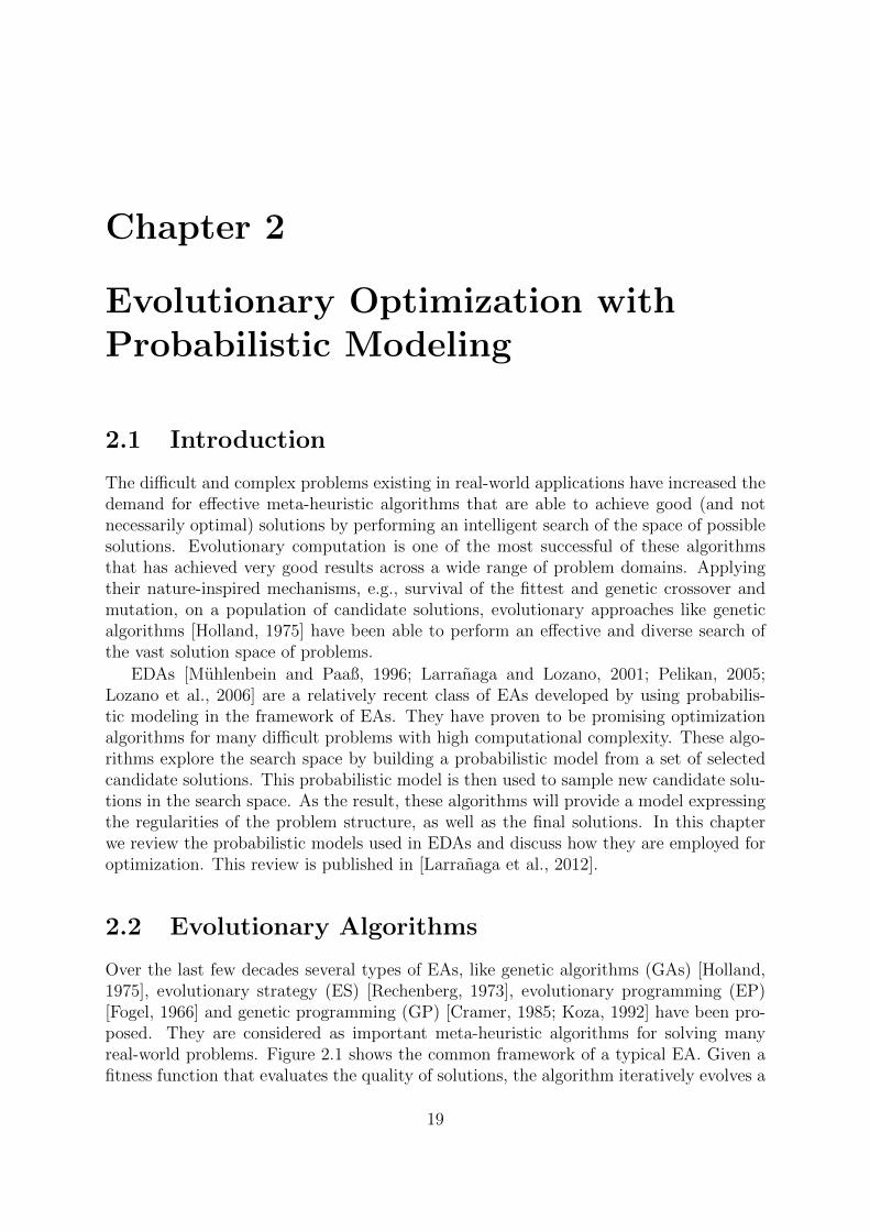
Figure 2.1: Flowchart of a typical evolutionary algorithm.

population of candidate solutions to the problem. Fitter solutions of the population areused to reproduce new offspring solutions (survival of the fittest principle) by applyinggenetic operators, i.e. crossover and mutation.

2.2.1 Genetic Algorithms

GAs are perhaps the most well-known and widely used EAs. Since their introduction[Holland, 1975], they have received an increasing amount of attention and interest, andnumerous works have studied their different aspects. A typical GA works by evolving apopulation of candidate solutions to the problem across a number of generations in orderto obtain better solutions. Solutions are usually represented as binary strings, the same asthe representation of information in machine language. The algorithm, selects a subset offitter solutions from the population according to a selection mechanism, e.g. tournamentselection, as the parents. These parent solutions reproduce new offspring solutions byapplying genetic operators like crossover and mutation. The newly generated solutionsthen compete for survival with the solutions in the population according to their fitnesses.

The simple and easy to understand mechanism of GAs with their simple solutionrepresentation method, has led to their intensive utilization for optimization in a vastvariety of domains, from engineering tasks [Gen and Cheng, 2000] to medicine [Alander,2012]. They have been also extensively used in multi-objective [Deb, 2001], uncertain anddynamic [Goh and Tan, 2009] domains under the general term of evolutionary algorithms.Despite their simple mechanics, several works have also studied the performance of thesealgorithms from a theoretical point of view [Holland, 1975; Harik et al., 1999a]. Forfurther information on these algorithms see [Goldberg, 1989, 2002].

2.2.2 Evolutionary Strategy

ES is one of the early types of EAs designed mainly to deal with continuous domainoptimization. A typical ES is specified by two parameters λ and µ which respectivelydetermine the population size and the parents size after applying selection. The mainevolutionary operator in this algorithm is mutation, applied together with the selectionoperator to continue the search. Since the size of the search space in continuous opti-mization is infinite, ES algorithms usually use smaller population sizes and larger numberof generations to evolve the solutions toward the optimum. More details about this typeof EAs can be found in [Schwefel, 1995; Beyer, 2001; Beyer and Schwefel, 2002].

20

2.2.3 Genetic Programming

The objective of GP is to evolve functions or computer programs to obtain a desiredfunctionality. The main difference of GP and GA is in the way that the solutions are rep-resented. The usual representation used to encode the solutions in GP is tree structures,where operations are shown as intermediate nodes and operands as terminal nodes of thetree. GP evolves a population of these trees in the general framework of EAs, tryingto generate programs that can better achieve the required functionality. In a broaderperspective, GP can be used for automatic generation of new content.

To deal with program-tree representation of solutions, the genetic operators usedto reproduce new solutions should be adapted accordingly. Crossover usually involvesswitching the compatible branches of two solutions. In mutation the values of specifictree nodes or a branch of the tree is changed (while respecting the compatibility of thewhole solution). Therefore, the solutions in the population can have different sizes. GPand EP are closely related and usually used interchangeably, with the latter putting moreemphasis on mutation in the generation of new solutions. The interested reader is referredto the series of books by Koza [Koza, 1992, 1994; Koza et al., 1999, 2003].

2.2.4 Complementary Methods

In order to improve the performance of EAs in optimization, several methods have beenproposed which modify or add to the general framework of EAs. Here we briefly introducetwo of these methods that have been employed to enhance the optimization performanceof EAs in some of the applications discussed later in this thesis.

Hybridization

Hybridization of an algorithm usually refers to the case where this algorithm is used inconjunction with a different type of method, and thus can cover various types of hybridiza-tion between different algorithmic frameworks. The most likely type of hybridization forEAs, is to use a local search method for improving new solution reproduction, which issometimes referred to as memetic algorithms [Hart et al., 2005]. In these algorithms aftergenerating a new solution using genetic operators, its local neighborhood is searched forfitter solutions using a local search method like hill climbing. This type of hybridizationcan improve the exploitation ability of EAs in search for optimal solution(s).

Cooperative Coevolution

Co-evolutionary algorithms are an extension to the original EAs and are specially designedfor optimization problems in complex systems. In coevolution, the fitness of each solutionis determined by the way it interacts with other solutions in the population. Basically,two types of coevolution can be considered: competition and cooperation. In competitivecoevolution [Stanley and Miikkulainen, 2004], the increase in the fitness of an individualnegatively affects the fitness of other solutions. Cooperative coevolution, on the otherhand, rewards those solutions that have better collaboration with other solutions [Potteret al., 1995]. In this type of coevolution, usually the problem is decomposed into anumber of subproblems and the individuals in the population represent sub-solutions to

21

these subproblems. Therefore these subsolutions need to cooperate with each other toobtain complete solutions with higher fitness values. The sub-solutions can be eitherevolved in different populations or in a single population, known as Parisian approach[Ochoa et al., 2008].

2.3 Estimation of Distribution Algorithms

A key to the success of EAs is the identification, preservation and effective combination ofthe fitter partial solutions to the problem during evolution [Harik et al., 1999a]. However,it has been shown that the operators used in traditional EAs fail to properly accomplishthis task when certain characteristics are present in the problem. A main reason forthis shortcoming is that these algorithms do not properly consider the dependencies andrelationships between the variables of the problem, and are not able to thoroughly exploitthe information obtained so far, up to the current stage of the search, in order to speedup convergence. There are properties like non-linearity, ill-conditioning and deception inreal world problems that without considering them, traditional EAs can have significantchallenges for optimization.

Probabilistic modeling offers a systematic way of acquiring this kind of regularities,and therefore can help to achieve a quick, accurate and reliable problem solving [Goldberg,2002; Pelikan et al., 2002]. EDAs try to overcome the shortcomings of traditional EAsby incorporating probabilistic modeling. For this purpose, instead of genetic operatorsused in traditional EAs, new candidate solutions to the problem in each iteration aregenerated using the following two steps:

1. Estimating a probabilistic model based on the statistics collected from the set ofcandidate solutions, and

2. Sampling the estimated probabilistic model.

In this way the problem regularities encoded in the probabilistic model are used whengenerating new solutions. Algorithm 2.1 shows the basic steps of an EDA. Worthy of noteis that probabilistic models can also be used in EAs for other purposes. For instance,to make decisions on the application of mutation operators, to assess the influence ofthe different EA parameters on the algorithm behavior, to obtain an estimation of solu-tion qualities without direct fitness evaluation, or even to implement local optimizationprocedures.

Implicitly, EDAs assume that it is possible to model the promising areas of the searchspace, and to use this model to guide the search for the optimal solution(s). The proba-bilistic model learnt in EDAs captures an abstract representation of the features sharedby the selected solutions and encodes the different patterns of interactions between sub-sets of the problem variables. Probabilistic modeling gives EDAs an advantage over othernon-model based EAs by allowing them to deal with problems containing important in-teractions among their variables. This, together with their capacity to solve differenttypes of problems in a robust and scalable manner [Pelikan, 2005; Lozano et al., 2006],has popularized these algorithms, which are sometimes even referred to as competentGAs [Goldberg, 2002; Pelikan et al., 2002] to differentiate them from traditional GA

22

Estimation of Distribution AlgorithmInputs:

A representation of solutions,An objective function f

1 P0 ← Generate initial population according to the given representation2 F0 ← Evaluate each individual x of P0 using f3 g ← 14 while termination criteria not met do5 Sg ← Select a subset of Pg−1 according to Fg−1 using a selection mechanism6 ρg(x)← Estimate the probability of solutions in Sg7 Qg ← Sample ρg(x) according to the given representation8 Hg ← Evaluate Qg using f9 Pg ← Replace Qg in Pg−1 according to Fg−1 and Hg

10 Fg ← Update Fg−1 according to the solutions in Pg11 g ← g + 112 end while

Output: The best solution in Pg−1

Algorithm 2.1: The basic steps of an estimation of distribution algorithm

algorithms. The successful application of EDAs to many real-world problems in differ-ent domains like: machine learning Inza et al. [2000, 2001a], bioinformatics Armananzaset al. [2008]; Santana et al. [2010c]; Armananzas et al. [2011], scheduling Zhang and Li[2011]; Wang and Fang [2012]; Chen and Chen [2013], industrial design and managementSun et al. [2008]; Jiang et al. [2006], protein folding Santana et al. [2007, 2008], softwaretesting Sagarna and Lozano [2006] and composite materials Grosset et al. [2006] haveproved their usefulness in practice. There are also many EDA implementations avail-able online, providing a range of possibilities for the application of EDAs to real-worldproblems [Santana, 2011].

Because of the different nature of both optimization and probabilistic modeling indiscrete and continuous domains, EDAs developed for each of these domains also havedifferences depending on the representation type they use for the problem. Therefore, inthe following sections each of these two categories are discussed separately. Here, we donot intend to give an exhaustive list of all proposed EDAs. Rather the aim is to review thedifferent probabilistic models and machine learning methods employed in EDAs. Anothercommon way of categorizing EDAs is by the complexity of the probabilistic models theyuse. In general, one of the rationales in EDA development has been to find a satisfactorytrade-off between the complexity of the probabilistic models they use and how accuratelythese models represent particular optimization problem characteristics. This is anotherfactor taken into account in reviewing EDAs here. Moreover, for readability we use thealgorithm acronyms. Table 2.1 lists the algorithms full names. For recent review paperson EDAs, the interested reader is referred to [Hauschild and Pelikan, 2011; Larranagaet al., 2012].

23

2.3.1 Discrete EDAs

Early EDAs were developed for discrete and especially binary domains, as it is a commonpractice in EAs to represent problem solutions with bit strings. Univariate EDAs, suchas PBIL [Baluja, 1994], cGA [Harik et al., 1999b] and UMDA [Muhlenbein and Paaß,1996], assume that all variables are independent and thus their joint probability can befactorized as a product of univariate marginal probabilities. The probabilistic model inthis case consists of separate nodes containing the probability distribution for each ofthe problem variables. While some algorithms (e.g., PBIL and UMDA) learn the modelfrom a population of solutions, others (e.g., cGA) update the model using only a fewindividuals. Consequently, these algorithms are the simplest EDAs and thanks to theirsimplicity, univariate EDAs are particularly suitable for the theoretical analysis of EDAbehavior [Gonzalez et al., 2002; Zhang, 2004].

To extend the modeling capability of EDAs, bivariate models were used in EDAs.Bivariate models can represent pairwise dependencies between variables using efficientlearning methods. MIMIC [De Bonet et al., 1997] uses a chain structured probabilisticmodel where the probability distribution of all the variables except the head node isconditioned on the value of the variable preceding them in the chain. The structureof the probabilistic model in COMIT [Baluja and Davies, 1997] is a tree, while it isgeneralized to a forest of trees (dependency graph) in BMDA [Pelikan and Muhlenbein,1999].

In univariate and bivariate EDAs, the probabilistic model structure is either fixed oris very restricted. Therefore, while they can be efficiently applied to separable problems(without any dependency) or to problems with low degrees of dependency among thevariables, they might still rapidly lose their efficiency when applied to more complicatedproblems, with larger number of variable interactions. A further attempt to improveEDAs is to use models that can capture dependencies between an arbitrary numberof variables. Thus the joint probability distribution can be decomposed into factorsinvolving several variables of the problem. Of course, this more flexible modeling bymultivariate EDAs, capable of learning complex structures, comes at the cost of a greatercomputational effort. Figure 2.2 shows some examples of possible model structures ofdifferent complexity learnt by EDAs.

Multivariate EDAs

FDA [Muhlenbein and Mahnig, 1999; Muhlenbein et al., 1999] gives a factorization of thejoint probability distribution for a class of problems known as additively decomposablefunctions. EcGA [Harik et al., 2006] factorizes the joint probability distribution into anumber of marginal distributions defined over non-overlapping subsets of variables in aprobabilistic model called marginal product model (MPM). An MDL scoring metric isused to search for the proper partitioning of the variables.

EBNA [Etxeberria and Larranaga, 1999] and BOA [Pelikan et al., 1999] learn a BNfrom the selected set of solutions in every generation. While both of the algorithms use agreedy local search method to explore the space of possible BN structures, EBNA mea-sures the quality of the structures using the BIC metric and BOA utilizes the BDe metricto score them. BOA is also further extended to hierarchical BOA [Pelikan, 2005] by incor-porating diversity-preserving techniques and an improved representation for BN parame-

24

(a) Univariatestructure

(b) Chain structure (c) Tree structure (d) Forest structure

(e) FDA model structure (f) EcGA modelstructure

(g) EBNA, BOAmodel structure

Figure 2.2: Examples of different types of model structures used in EDAs.

ters using decision graphs. An improved version of FDA, known as learning FDA, is alsoproposed that uses BNs to dynamically learn the interdependent variables [Muhlenbeinand Mahnig, 1999]. Thanks to the powerful probabilistic model that these algorithmsuse, they can be applied to solve many difficult problems [Larranaga et al., 2000b; Pelikanand Hartmann, 2006].

Because of the model learning complexity in general, MN-based EDAs [Santana, 2003;Wang and Wang, 2004; Shakya, 2006; Alden, 2007] are usually applied to applicationswhere the structure of the optimization problem is known and can be easily representedusing an undirected graphical model. However, an approximation of the probabilitydistribution, like Kikuchi approximations [Santana, 2005], can also be estimated to obtainthe factorization of problem variables. The use of this type of probabilistic models foroptimization is still topic of active research and very recently Shakya and Santana [2012]have reviewed the new developments in this type of EDAs.

EDNA [Gamez et al., 2007] uses dependency networks [Heckerman et al., 2001] tomodel the problem structure. Based on a heuristic approximation, this algorithm usessecond-order statistics (similar to bivariate EDAs) for model learning. Dependency net-works can represent cyclic dependencies between variables which cannot be encoded inBNs. However, this property prevents the application of sampling techniques used for BNslike PLS method. Therefore, similar to MN-based EDAs, EDNA uses relatively complexGibbs sampling [Geman and Geman, 1984] procedures to generate new solutions from

25

the probabilistic model.

Other Modeling Types

Apart from basic probabilistic models, EDAs have also used other modeling techniques.Mixture of models increases the flexibility of joint probability estimation in EDAs, espe-cially for solving multi-modal optimization problems (containing several optima). Pelikanand Goldberg [2000] studied the effect of clustering the set of selected solutions on theperformance of UMDA. UEBNA [Pena et al., 2005] represents the mixture with a BNwhich is learnt by the structural EM algorithm. Santana et al. [2009b] discussed severaltopics concerning model building in discrete EDAs.

A promising technique is to take into account the fitness information of individuals inthe modeling process. EBCOA [Miquelez et al., 2004] adopts this idea, first introduced byMichalski [2000], by dividing the set of selected individuals into different classes accordingto their fitness values. The probabilistic model of this algorithm can be any of the BNclassifiers (Section 1.3.4) with the class node corresponding to the different levels offitness values (after discretization). Similarly, Shakya and McCall [2007] directly usedthe fitness values in the estimation of MN parameters in their proposed DEUM framework[Shakya, 2006], assuming that the probability of each solution in the search space canbe approximated by its fitness value. Another related idea is to learn EDA probabilitydistributions from both low and high fitness individuals [Hong et al., 2009]. Valdez-Penaet al. [2009] have extended this idea by estimating a distribution for selection operatorsand used it to identify which solutions would be used for model learning.

Probabilistic models in EDAs can also be used to estimate or predict the fitnessvalues of the new solutions. This approach can be especially useful for problems witha very difficult and time-consuming fitness function. Fitness inheritance modeling hasbeen incorporated into EcGA [Sastry et al., 2004] and BOA [Pelikan and Sastry, 2004] toestimate the fitness value of new individuals and, consequently, reduce the total numberof function evaluations consumed by the algorithm to reach the optimum. Brownlee et al.[2008] and Brownlee [2009] used a MN-based fitness model in DEUM to predict the fitnessvalue of the new individuals and also compare their correlations to the true fitness values.

Propagation methods, used for inference in BNs, also have applications in EDAs.Mendiburu et al. [2007] used total abductive inference to find the most probable value-setting of BN variables, as one of the solutions generated from the probabilistic model inEBNA to improve the sampling procedure. Lima et al. [2009] used loopy belief propaga-tion in a local search method in BOA as a way to compute optimal local value-settingsof the problem. An analysis of EBNA performance at different stages of evolution isalso given by computing the most probable value-setting at each generation [Echegoyenet al., 2009]. AffEDA [Santana et al., 2010b] uses affinity propagation [Frey and Dueck,2006], another propagation algorithm based on probabilistic modeling, to obtain non-overlapping factorizations of the joint probability distribution.

There have been also attempts to hybridize EDAs with other optimization algorithms,like differential evolution [Sun et al., 2005] and artificial immune systems [de Castro andZuben, 2009]. Recently, Bengoetxea and Larranaga [2010] and Ahn et al. [2012] have pro-posed very similar frameworks for hybridizing EDAs with particle swarm optimization, incontinuous and discrete domains respectively. The central idea of these techniques is to

26

combine the global search ability of EDAs with better local exploitation of other meth-ods. LTGA [Thierens, 2011] takes advantage of structure learning in EDAs and geneticrecombination in GAs by building a linkage tree using an agglomerative hierarchical clus-tering algorithm with mutual information as its distance metric. Using this linkage treethe algorithm determines the crossing point of the parents when applying the crossoveroperator to the selected solutions for generating new solutions.

2.3.2 Continuous EDAs

The usual choice, adopted by most EAs in continuous domain optimization, is to assumea Gaussian distribution for problem variables. Many of the early continuous EDAs aswell as their recent improvements are also based on this assumption. PBILC [Sebag andDucoulombier, 1998] extends its discrete version to continuous domains by updating avector of independent Gaussian distributions. UMDAC [Larranaga et al., 1999, 2000a]uses ML estimation to learn the parameters of the Gaussian distribution for each variablefrom the population of solutions. MIMICC [Larranaga et al., 1999, 2000a] learns thechain structured probabilistic model for continuous variables by adapting the concept of(conditional) entropy for univariate and bivariate Gaussian distributions.

EGNA [Larranaga et al., 1999, 2000a; Larranaga and Lozano, 2001] can be consideredas the continuous version of EBNA based on a GBN. Two approaches have been proposedfor learning the network structure in this algorithm: (i) starting from a complete DAG,likelihood ratio hypothesis tests are used to decide whether the edge between two nodesshould be excluded from the network; (ii) performing a greedy local search in the spaceof possible DAGs using a scoring metric like BGe (continuous version of the BDe metric)or BIC. EBCOA has also been extended to continuous domains [Miquelez et al., 2006]by building BN classifiers that assume Gaussian distributions for the variables given theclass variable value. Karshenas et al. [2011b] proposed learning a joint GBN consistingof both variables and objectives in their JGBN-EDA for multi-objective optimization.

IDEA [Bosman and Thierens, 2000a,b] and EMNA [Larranaga and Lozano, 2001] learnan MGD from the set of selected solutions. While EMNA uses ML estimation, IDEAemploys Kullback-Leibler divergence in conjunction with a greedy search algorithm, aswell as likelihood ratio statistical hypothesis tests. Further improvements of IDEA havebeen proposed by scaling the diminishing variances [Grahl et al., 2006] and shifting thedistribution mean [Bosman and Grahl, 2008; Bosman et al., 2008].

Mixture of Distributions

An extended version of IDEA [Bosman and Thierens, 2001] uses a mixture of normaldistributions over clusters of solutions, obtained by applying a clustering algorithm beforelearning mixture components. rBOA [Ahn et al., 2004] first learns a GBN to obtaina decomposition of the problem variables into smaller subproblems. Then, a separatemixture of GBNs is learnt for each of the subproblems by clustering the solutions inthat subproblem. In BGMMEDA [Li et al., 2006], instead of clustering the samples, aboosting technique is applied to estimate a Gaussian mixture model.

MB-GNG [Martı et al., 2011] adopts growing neural gas, a specific single-layer neuralnetwork, to determine the location of the components of the mixture of Gaussian distri-

27

butions. This model learning algorithm is sensitive to, and therefore does not neglect,outliers and is able to automatically adapt its topology while decreasing the accumu-lated error of the network nodes. The multi-model EDA framework [Weise et al., 2011]extends these mixture methods by applying traditional EA recombination operators tothe individual models learnt for each of the clusters in order to improve search spaceexploration. RM-MEDA [Zhang et al., 2008] learns a piece-wise continuous manifoldfor multi-objective optimization using the local principle component analysis algorithm.Each model component is a hyper-rectangle with an added Gaussian noise.

Other Modeling Approaches

Posık [2008, 2009] proposed the use of Cauchy distribution for the purpose of preventingpremature convergence. Since the moments of an n-dimensional variable with multivari-ate Cauchy distribution are not defined, the mean vector and covariance matrix of anMGD are computed instead. For sampling new solutions, the scaling factor of the Cauchydistribution is used to obtain isotropically distributed new solutions.

More recently some EDAs have employed copula theory to relax the Gaussian as-sumption for the variables. Copula-based EDAs (CEDAs) [Salinas-Gutierrez et al., 2009;Wang et al., 2009; Wang and Zeng, 2010; Cuesta-Infante et al., 2010] use the copulafunction for estimating the joint probability distribution of the variables according toSklar’s theorem. The copula function only uses the marginal univariate probabilities tocompute the joint probability distribution. This reduces the computational complexityof model learning. Two-dimensional elliptical copulas as well as Archimedean and em-pirical copulas and their extensions to higher dimensions are studied in the literature.These copula functions provide the variable interaction structure of the problem whensampling new solutions from the learnt model. In each generation the algorithm selectsor constructs a copula function after estimating the univariate marginal distributions andthen, generates new samples according to the copula distribution.

CMA-ES [Hansen, 2006] incorporates model estimation into ES. The algorithm learnsan MGD as its probabilistic model to generate new solutions. The probabilistic modelestimated in each generation is a combination of information collected over several gen-erations, taking into account the path that the optimizer has traversed in the searchspace (the gradient information). Instead of estimating a new probabilistic model in eachgeneration, the algorithm adapts the model during evolution. Thus, the algorithm is ableto use smaller population sizes for optimization by spanning model learning over severalgenerations. Because of such an adaptation strategy, some researchers do not completelyconsider this algorithm as an EDA [Posık, 2009]. It is worth to note that similar tech-niques have been proposed for improving the efficiency of other EDAs in optimization[Pelikan et al., 2008; Bosman et al., 2008].

Non-parametric Probabilistic Models

Other probabilistic models that estimate a non-parametric probability distribution forthe variables have also been used in continuous EDAs. IDEA, for example, has employedother models, apart from MGD, like Gaussian kernel distribution (a Gaussian kernel foreach sample) or histograms in its framework [Bosman and Thierens, 2000b,a].

28

Cho and Zhang [2002] proposed a continuous EDA that learns a mixture of factoranalyzers using EM algorithm. They also employed a more complicated mixture of vari-ational Bayesian independent component analyzers in a later study [Cho and Zhang,2004]. MOPEDA [Costa and Minisci, 2003] applies a Parzen estimator that convolvesthe empirical estimation obtained from a finite data set with a squared integrable kernelfunction in order to reduce the variance of the probability distribution estimation. BothGaussian and Cauchy kernels are used alternatively during evolution to utilize their in-trinsic complementary characteristics. In KEDA [Luo and Qian, 2009], the width of eachkernel is dynamically computed during the optimization.

Histogram-based EDAs (HEDAs) discretize each variable’s values by dividing theirrange to a number of bins. Tsutsui et al. [2001] proposed two types of marginal histogrammodels: (i) a fixed-width histogram (FWH) where the domain of each variable is dividedinto a fixed number of bins whose height may differ depending on the variable values; (ii)a fixed-height histogram (FHH) where all bins have an equal value generation probabilitybut can have different widths. Consequently, there will be more bins in denser regionsand thus modeling will be more accurate.

Ding et al. [2008] proposed two improvements to the above histogram modeling intheir HEDA. They introduced a surrounding effect, where the values of each bin canaffect the values of its surrounding bins using a special surrounding factor. They alsoemployed a shrinkage strategy where the height of the bin containing the best value ofthe variable can exceed a predefined threshold. PBILC is also extended with histograms[Xiao et al., 2009], combining the original updating rule with bin updating, where thebins reaching a predefined height are divided.

Histogram modeling has also been applied to optimization in permutation domains[Tsutsui, 2002; Tsutsui et al., 2006] using two different types of models. The first isan edge histogram matrix where each entry indicates the frequency of two permutationvalues occurring adjacent to each other in the population. The second is a node histogrammatrix that encodes the frequency at which a special value in the permutation occurs ata specific location in the solution. Specific sampling algorithms are developed for thesemodels where a new value is generated according to the value of adjacent permutationlocations or the position for which the value is going to be generated.

2.3.3 Discrete-Continuous EDAs

MBOA [Ocenasek and Schwarz, 2002; Ocenasek et al., 2004] adopts binary classificationand regression decision trees to solve mixed discrete-continuous optimization problems.The algorithm uses a BDe-like scoring metric to build a decision tree for each variableto encode its related probability distribution. The decision trees allow the algorithm tobuild individual models (like Gaussian kernels) for specific regions of the search space,stored in different tree leaves.

2.3.4 Discussion

Table 2.1 gives a summary of the presented EDAs and their probabilistic models. Thealgorithms are divided into three different classes according to the complexity of theirprobabilistic models: univariate, bivariate and multivariate EDAs. Within each class,

29

Table 2.1: Full name of EDAs and the models they use. Discrete EDAs are shown ona white, continuous on a green and mixed discrete-continuous on a blue background,respectively.

Univariate Bivariate Multivariate

Alg

ori

thm

Com

ple

teN

am

eM

od

el

Use

d

PB

ILP

opu

lati

onB

ased

Incr

emen

tal

Lea

rnin

g-

UM

DA

Un

ivar

iate

Mar

gin

alD

istr

ibu

tion

Alg

ori

thm

-

PB

ILC

Con

tinu

ous

PB

IL-

cGA

Com

pac

tG

enet

icA

lgor

ith

m-

UM

DA

CC

onti

nu

ous

UM

DA

-

HE

DA

His

togr

am-b

ased

ED

AM

arg

inal

His

togra

ms

MIM

ICM

utu

alIn

form

atio

nM

axim

izin

gIn

pu

tC

lust

erin

gC

hain

CO

MIT

Com

bin

ing

Op

tim

izer

sw

ith

Mu

tual

Info

rmati

on

Tre

esT

ree

BM

DA

Biv

aria

teM

argi

nal

Dis

trib

uti

on

Alg

ori

thm

Fore

st

MIM

ICC

Con

tinu

ous

MIM

ICC

hain

CE

DA

Cop

ula

-bas

edE

DA

Cop

ula

Fu

nct

ion

s

FD

AF

acto

rize

dD

istr

ibu

tion

Alg

ori

thm

Fact

or

Gra

ph

EB

NA

Est

imat

ion

ofB

ayes

ian

Net

work

Alg

ori

thm

Bay

esia

nN

etw

ork

BO

AB

ayes

ian

Op

tim

izat

ion

Alg

ori

thm

Bay

esia

nN

etw

ork

EG

NA

Est

imat

ion

ofG

auss

ian

Net

work

Alg

ori

thm

Gau

ssia

nB

ayes

ian

Net

work

IDE

AIt

erat

edD

ensi

tyE

stim

atio

nE

volu

tion

ary

Alg

ori

thm

Gau

ssia

nM

ark

ovN

etw

ork

EM

NA

Est

imat

ion

ofM

ult

ivar

iate

Norm

al

dis

trib

uti

on

Alg

ori

thm

Gau

ssia

nM

ark

ovN

etw

ork

MB

OA

Mix

edB

OA

Dec

isio

nG

rap

hs

MN

-FD

AM

arko

vN

etw

ork

bas

edF

DA

Mark

ovN

etw

ork

MO

PE

DA

Mu

lti-

Ob

ject

ive

Par

zan

-base

dE

DA

Mix

ture

of

Ker

nel

s

rBO

AR

eal-

cod

edB

OA

Gau

ssia

nB

ayes

ian

Net

work

EB

CO

AE

volu

tion

ary

Bay

esia

nC

lass

ifier

base

dO

pti

miz

ati

on

Alg

ori

thm

Bay

esia

nN

etw

ork

Cla

ssifi

ers

MN

-ED

AM

arko

vN

etw

ork

ED

AM

ark

ovN

etw

ork

UE

BN

AU

nsu

per

vis

edE

BN

AB

ayes

ian

Net

work

EcG

AE

xte

nd

edcG

AM

arg

inal

Pro

du

ctM

od

el

BG

MM

ED

AB

oos

tin

gG

auss

ian

Mix

ture

Mod

elb

ase

dE

DA

Mix

ture

of

Gau

ssia

nM

ark

ovN

etw

ork

s

DE

UM

Dis

trib

uti

onE

stim

atio

nU

sin

gM

ark

ovR

an

dom

Fie

lds

Mark

ovN

etw

ork

CM

A-E

SC

ovar

ian

ceM

atri

xA

dap

tati

on

Evolu

tionary

Str

ate

gy

Gau

ssia

nM

ark

ovN

etw

ork

MA

RL

ED

AM

arko

via

nL

earn

ing

ED

AM

ark

ovN

etw

ork

ED

NA

Est

imat

ion

ofD

epen

den

cyN

etw

ork

Alg

ori

thm

Dep

end

ency

Net

work

RM

-ME

DA

Reg

ula

tory

Mod

el-B

ased

Mu

lti-

Ob

ject

ive

ED

AM

ixtu

reof

hyp

erp

lan

es

KE

DA

Ker

nel

den

sity

-bas

edE

DA

Mix

ture

of

Gau

ssia

nK

ern

els

Aff

ED

AA

ffin

ity

pro

pag

atio

nE

DA

Marg

inal

Pro

du

ctM

od

el

MB

-GN

GM

od

elB

uil

din

gG

row

ing

Neu

ral

Gas

Mix

ture

of

Gau

ssia

nM

ark

ovN

etw

ork

s

LT

GA

Lin

kage

Tre

eG

AH

iera

rch

ical

Dep

end

ency

Tre

e

JG

BN

-ED

AJoi

nt

GB

N-b

ased

ED

AG

au

ssia

nB

ayes

ian

Net

work

30

the algorithms are ordered chronologically to show how the use of probabilistic modelsin EDAs has evolved during time.

Initial EDAs mainly considered about the probability distribution of individual vari-ables, in order to perform a more effective search for the solutions of separable problems.In this kind of problems the optimal value of each variable can be obtained regardless ofthe value of the other variables. In other terms, the way that the value of each variableinfluences the fitness of the whole solution is not affected by the values of other variablesat all.

The limitations of univariate EDAs, brought up the need for a more advanced prob-abilistic modeling. The main advantage of these new probabilistic models is that theyconsider a kind of structure for the problem, reflecting an estimation of the interactionsbetween variables. Some algorithms put certain constraints on the structures, e.g. bi-variate EDAs can only consider mutual interactions. Some others like FDA consider afixed structure given beforehand (e.g. for a specific class of problems), and try to findthe best parameter estimation that fits this structure. But most of EDAs try to learn thestructure dynamically during evolution. A number of algorithms require the variablesto be clustered into completely disjoint dependence groups (e.g. EcGA and AffEDA),whereas in others overlapping groups of dependent variables is allowed (e.g. MIMIC andEBNA).

Because of their ability to represent complex patterns of interactions between theproblem variables, the use of multivariate probabilistic models has become dominant inEDAs. Usually these algorithms perform a kind of structure learning to estimate theprobabilistic model, which is very time-consuming in comparison to other parts of thealgorithm. Therefore, in practice an upper bound is imposed on the order of interac-tions that is considered in the structure learning. This restriction can also be imposedimplicitly, e.g. using penalized scoring metrics for learning BNs (Section 1.3.3).

The choice of the type of EDA to be used, depends very much on the problem. If theproblem at hand is linear, or the variables are not believed to be strongly dependent, thenone should use univariate EDAs since they are computationally more efficient. On thecontrary, if we are dealing with a problem that has high order of interactions between itsvariables, then EDAs that use probabilistic models with higher representational capabilityshould be used in order to be able to reach the optimal solution(s) of the problem. Thestructures estimated by these EDAs can also give a better understanding of unknownproblems. Several works have studied the accuracy of these structures and the informationwe can obtain from them [Lima et al., 2007; Karshenas et al., 2009; Santana et al., 2009a].

In reality, one should compromise between the computational complexity and theoptimization capability of these algorithms when applying them to different problems.Based on this observation, there has been many efforts to increase the efficiency of EDAswhile keeping their complexity at an acceptable range. Techniques like parallelizationand hybridization (discussed in Section 2.2.4) are introduced in the literature which areusually referred to as efficiency enhancement techniques [Pelikan, 2005].

2.3.5 Model-Based Genetic Programming

Although probabilistic models were first built into GAs, the idea was soon adopted also inGP. Because of the complex solution representation used in GP, model learning and sam-

31

pling can be a challenging task. However, several GP algorithms based on probabilisticmodeling have been proposed in the literature.

Probabilistic incremental program evolution (PIPE) [Sa lustowicz and Schmidhuber,1997] is a GP algorithm based on univariate factorization of program distribution. Aprobabilistic prototype tree (PPT) model encodes the probability distribution and islater used to generate new program trees at each generation of the algorithm. Extendedcompact genetic programming (ECGP) [Sastry and Goldberg, 2003] incorporates the useof marginal product distributions into the context of GP. Also based on a PPT model,ECGP constructs a factorization of the tree program distribution equal to the productof marginal distributions. Each marginal distribution is associated with a subtree of thePPT. The structure of the factorization is learned using a greedy algorithm, similar toEcGA.

The use of BNs for GP was proposed by Yanai and Iba [2003]. This estimation ofdistribution programming approach is based on the use of the PPT. The conditionalprobabilities between the nodes of the PPT are computed for the purpose of representinga wider class of probability distributions than PIPE and ECGP. More recently, Hasegawaand Iba [2008] proposed a BN modeling approach for GP that significantly reduces thesize of the conditional probability tables. The algorithm also requires fewer samples toconstruct the BN from the selected solutions.

Another type of model-based GP algorithms involve the use of grammars. Thesealgorithms [Shan et al., 2006; McKay et al., 2010; Bosman and de Jong, 2008] departfrom the traditional uses of PGMs since the probability distributions are often associatedwith the grammar rules and their different contexts of application. For example, Bosmanand de Jong [2008] estimate the distribution of programming trees based on the subtreesthat actually occur in the data. The representation specifies a set of rules whose expansionleads to trees, and the probability distributions are defined on these rules. For a reviewof these algorithms, see [Shan et al., 2006] and [McKay et al., 2010].

2.4 Conclusions

One of the disciplines that has greatly taken advantage of probabilistic modeling is evo-lutionary computation, resulting in a new class of algorithms which are called estimationof distribution algorithms. Although this is a relatively new paradigm, numerous stud-ies have investigated their different aspects, and several types of algorithms have beenproposed based on this paradigm. These algorithms cover both discrete and continuousdomains, and within each domain probabilistic models with different complexities havebeen used.

EDAs are still a topic of intensive research, and every year many new works relatedto the theory or application of these algorithms are published. New studies are trying toextend the application of these algorithms to other domains like multi-objective, noisy ordynamic problems. Nevertheless, because of the close relationship that these algorithmshave with probabilistic modeling, any new development in the area of probabilistic mod-eling, specially regarding the efficiency of the learning and sampling methods, can helpto achieve competent problem optimization with EDAs.

32

Chapter 3

Evolutionary Algorithms in BayesianNetwork Inference and Learning

3.1 Introduction

Some of the most relevant inference and learning problems in Bayesian networks areformulated as the optimization of a function. These problems usually have an intractablecomplexity and therefore are a potential domain for the application of meta-heuristicmethods. In the previous chapter we discussed how PGMs and in general probabilisticmodeling is used in EA framework to improve the optimization performance in EDAs.However, this collaboration has not been all one-sided, and EAs have also been extensivelyapplied to solve many optimization tasks in PGMs and especially in BNs. In this chapterwe review how EAs have been applied for solving some of the combinatorial problemsexisting in the inference and learning of BNs. This review is published in [Larranagaet al., 2013].

3.2 Triangulation of the Moral Graph

Lauritzen and Spiegelhalter [1988] proposed one of the most popular algorithms for exactinference in BN. The first step of this algorithm is to moralize the BN structure. In thisstep all variables with a common child are linked together and then all edge directions areremoved. The resulting graph is called a moral graph. The second step of the algorithmis the so-called triangulation of the moral graph. A graph is triangulated if any cycle oflength greater than 3 has a chord. This step is considered as the hardest step (in termsof computational complexity) of this inference algorithm. The resulting structure is thenused for evidence propagation and probability computation.

The basic technique for triangulating a moral graph (see also Figure 3.1) is throughsuccessive elimination of graph nodes. Before eliminating a node and its incident edges,we check that all of its adjacent nodes are directly connected to each other by adding therequired edges to the graph. The nodes are chosen for elimination according to a givenorder of the variables. The quality of a triangulation is measured by the weight of the

33

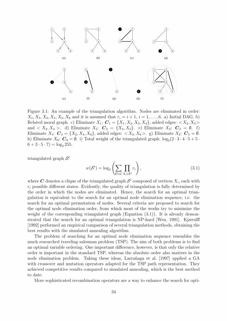
1

3 4

2

5 6

(a)

1

3 4

2

5 6

(b)

2

3 4

2

5 6

(c)

1

3 4

6

(d)

5

4

2

6

(e)

3

6

(h)

2

6

4

(f)

6

2

(g)

1

3 4

2

5 6

(i)

Figure 3.1: An example of the triangulation algorithm. Nodes are eliminated in order:X1, X5, X3, X4, X2, X6 and it is assumed that ri = i+ 1, i = 1, . . . , 6. a) Initial DAG. b)Related moral graph. c) Eliminate X1: C1 = {X1, X2, X3, X4}, added edges: <X2, X3>and < X3, X4 >. d) Eliminate X5: C2 = {X4, X5}. e) Eliminate X3: C3 = ∅. f)Eliminate X4: C4 = {X2, X4, X6}, added edges: <X2, X6>. g) Eliminate X2: C5 = ∅.h) Eliminate X6: C6 = ∅. i) Total weight of the triangulated graph: log2(2 · 3 · 4 · 5 + 5 ·6 + 3 · 5 · 7) = log2 255.

triangulated graph St

w(St) = log2

(∑C∈C

∏Xi∈C

ri

), (3.1)

where C denotes a clique of the triangulated graph St composed of vertices Xi, each withri possible different states. Evidently, the quality of triangulation is fully determined bythe order in which the nodes are eliminated. Hence, the search for an optimal trian-gulation is equivalent to the search for an optimal node elimination sequence, i.e. thesearch for an optimal permutation of nodes. Several criteria are proposed to search forthe optimal node elimination order, from which most of the works try to minimize theweight of the corresponding triangulated graph (Equation (3.1)). It is already demon-strated that the search for an optimal triangulation is NP-hard [Wen, 1991]. Kjærulff[1992] performed an empirical comparison of several triangulation methods, obtaining thebest results with the simulated annealing algorithm.

The problem of searching for an optimal node elimination sequence resembles themuch researched traveling salesman problem (TSP). The aim of both problems is to findan optimal variable ordering. One important difference, however, is that only the relativeorder is important in the standard TSP, whereas the absolute order also matters in thenode elimination problem. Taking these ideas, Larranaga et al. [1997] applied a GAwith crossover and mutation operators adapted for the TSP path representation. Theyachieved competitive results compared to simulated annealing, which is the best methodto date.

More sophisticated recombination operators are a way to enhance the search for opti-

34

Table 3.1: Application of evolutionary algorithms to inference in Bayesian networks

Task Reference Representation AlgorithmT

rian

gu

l.

Larranaga et al. [1997] Permutation of Variables GA

Wang et al. [2006] Permutation of Variables GA

Romero and Larranaga [2009] Permutation of Variables REDA

Dong et al. [2010b] Permutation of Variables GA

MP

E

Gelsema [1995] Value-setting for Variables GA

Rojas-Guzman and Kramer [1996] Graph GP

Mengshoel [1999] Value-setting for Variables GA

Sriwachirawat and Auwatanamongkol [2006] Value-setting for Variables GA

MA

P de Campos et al. [1999] Value-setting for Variables GA

de Campos et al. [2001] Value-setting for Variables UMDA, MIMIC, EBNA

mal variable ordering. Wang et al. [2006] proposed an adaptive GA able to self-adapt thecrossover and mutation operators probabilities, and provided a ranking-based selectionoperator that adjusts the pressure of selection according to the population evolution. Re-cently, Dong et al. [2010b] proposed a new GA based on a new rank-preserving crossoveroperator and a two-fold mutation mechanism that utilizes the minimum fill weight heuris-tic.

Another alternative to improve search efficiency for this problem has been to useprobabilistic modeling. Romero and Larranaga [2009] proposed an approach based onrecursive EDAs (REDAs) for both discrete and continuous representation of the variables.REDAs partition the set of vertices (that are to be ordered) into two subsets. In eachREDA call, the vertices in the first subset are fixed, whereas the other subset of variablesis evolved with a standard EDA. In the second call, the subsets switch roles.

The research on this problem so far has shown that GAs can obtain results comparableto simulated annealing. A very close behavior is seen when using REDAs, with improvedconvergence speed. The comparison with other types of optimization algorithms that useother optimization criteria also show that GAs which use the minimizing graph weight asthe optimization criterion can find better node elimination orders, provided that properoperators and parameters are used.

3.3 Total and Partial Abductive Inference

EAs have also been used to search for the MPE in a BN. Gelsema [1995] used a GA whereeach individual is a value-setting for the unobserved variables, i.e., a string of integers.Rojas-Guzman and Kramer [1996] employed a GP where each individual represents thewhole BN with all the nodes in the explanation set instantiated to one of their possiblestates. Mengshoel [1999] used a GA coupled with his proposed probabilistic crowdingreplacement to perform a more efficient search for the MPE by better preservation ofthe diversity. Sriwachirawat and Auwatanamongkol [2006] proposed a GA for solving themore complex problem of finding the k MPEs [Nilsson, 1998].

De Campos et al. [1999] proposed a GA for approximate partial abductive inference(MAP) given an evidence set. The individuals in the GA population represent a possible

35

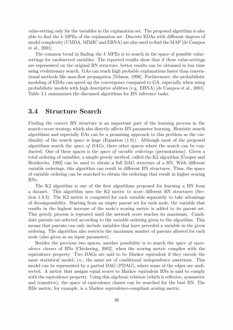
value-setting only for the variables in the explanation set. The proposed algorithm is alsoable to find the k MPEs of the explanation set. Discrete EDAs with different degrees ofmodel complexity (UMDA, MIMIC and EBNA) are also used to find the MAP [de Camposet al., 2001].

The common trend in finding the k MPEs is to search in the space of possible value-settings for unobserved variables. The reported results show that if these value-settingsare represented on the original BN structure, better results can be obtained in less timeusing evolutionary search. GAs can reach high probable explanations faster than conven-tional methods like max-flow propagation [Nilsson, 1998]. Furthermore, the probabilisticmodeling of EDAs can speed up the convergence compared to GA, especially when usingprobabilistic models with high descriptive abilities (e.g. EBNA) [de Campos et al., 2001].Table 3.1 summarizes the discussed algorithms for BN inference tasks.

3.4 Structure Search

Finding the correct BN structure is an important part of the learning process in thesearch+score strategy which also directly affects BN parameter learning. Heuristic searchalgorithms and especially EAs can be a promising approach to this problem as the car-dinality of the search space is huge (Equation (1.9)). Although most of the proposedalgorithms search the space of DAGs, there other spaces where the search can be con-ducted. One of these spaces is the space of variable orderings (permutations). Given atotal ordering of variables, a simple greedy method, called the K2 algorithm [Cooper andHerskovits, 1992] can be used to obtain a full DAG structure of a BN. With differentvariable orderings, this algorithm can result in different BN structures. Thus, the spaceof variable ordering can be searched to obtain the orderings that result in higher scoringBNs.

The K2 algorithm is one of the first algorithms proposed for learning a BN froma dataset. This algorithm uses the K2 metric to score different BN structures (Sec-tion 1.3.3). The K2 metric is computed for each variable separately to take advantageof decomposability. Starting from an empty parent set for each node, the variable thatresults in the highest increase of the node’s scoring metric is added to its parent set.This greedy process is repeated until the network score reaches its maximum. Candi-date parents are selected according to the variable ordering given to the algorithm. Thismeans that parents can only include variables that have preceded a variable in the givenordering. The algorithm also restricts the maximum number of parents allowed for eachnode (also given as an input parameter).

Besides the previous two spaces, another possibility is to search the space of equiv-alence classes of BNs [Chickering, 2002], when the scoring metric complies with theequivalence property. Two DAGs are said to be Markov equivalent if they encode thesame statistical model, i.e., the same set of conditional independence assertions. Thismodel can be represented by a partial DAG (PDAG), where some of the edges are undi-rected. A metric that assigns equal scores to Markov equivalent BNs is said to complywith the equivalence property. Using this algebraic relation (which is reflexive, symmetricand transitive), the space of equivalence classes can be searched for the best BN. TheBDe metric, for example, is a Markov equivalence-compliant scoring metric.

36

In this section, we review some of the EA-based methods proposed for BN structuresearch. Note that we focus our review on the EAs introduced in Chapter 2, which aremore relative to the line of research in this thesis, although some other evolutionaryapproaches like ant colony optimization have also been used for this task [de Camposet al., 2002]. The reviewed methods are divided into three categories depending on thespace where they perform the search for finding the best BN structure. The methods arealso listed in Table 3.2.

3.4.1 DAG Space

Larranaga et al. [1996c] proposed a GA that encodes the connectivity matrix of the BNstructure in its individuals. The algorithm, which uses a marginal likelihood-based metricto score the BN structures, considers two different approaches. In the first approach thereis a total ordering assumption between the variables (parents before children), and thusthe variation operators (one-point crossover and bit mutation) are closed. This restrictionalso reduces the cardinality of the search space. In the second approach, there is no suchassumption, and the algorithm should deal with a larger space. In this case, a repairingoperator is needed to ensure that the variation operators result in a valid BN structure.

To overcome the requirement for a repairing operator, Etxeberria et al. [1997] used thefuse-DAGs algorithm [Matzkevich and Abramson, 1992] to guarantee that the crossoveroperator satisfies the closure property. Larranaga et al. [1996b] hybridized two versionsof a GA with a local search operator to obtain better structures. Myers et al. [1999]extended the use of GAs for BN learning to domains with missing data, simultaneouslyevolving the structure of the BN and the missing data in separate populations. At eachgeneration the new solutions generated in both populations are used to compute the BDescore of each network structure.

Cotta and Muruzabal [2002] built phenotypic information into gene-based and allele-based recombination operators in a GA to search for the best structure according toa penalized likelihood-based scoring metric. Using guidelines on how GAs work [Hariket al., 1999a], van Dijk et al. [2003] designed a GA where the recombination operator triesto prevent the disruption of the good BN substructures obtained so far in the population.The algorithm uses an MDL metric as the fitness function for scoring the network struc-tures, and a repairing operator to ensure that structures are acyclic. In the domains withmixed discrete-continuous variables, Mascherini and Stefanini [2005] proposed a mixedGA to search for the optimal CGN, where invalid structures are corrected by deletinginadmissible arcs at random. An extension of the BDe metric is used to measure thefitness of the model for the mixed domain dataset.

Blanco et al. [2003] compared the performance of GAs with two univariate EDAs,namely, UMDA and PBIL, using three different scoring metrics. The reported results,both with and without a total ordering assumption between variables, showed that EDAsare able to obtain better or comparable BN structures. Kim et al. [2005] used fitnesssharing in an EA to obtain a diverse population of BN structures. The BNs learnt at theend of evolution are then combined according to Bayes’ rule for providing a more robustinference.

Hanzelka [2008] also proposed a hybridization of GA with local search methods per-formed on single solutions under the term of Lamarckian evolution. It uses a Chi-squared

37

test to determine the edges that should be removed for repairing the structure. After GAterminates, an additional exhaustive search is conducted in the most promising subspaceof BN structures found.

Barriere et al. [2009] proposed an EA which uses a cooperative coevolution strategyto evolve a population of conditional independence assertions. The scoring criteria is theChi-squared test. At the end of evolution, the best conditional independence assertionsfound (partly stored in an archive) are used to build the structure of the BN.

The EP algorithm proposed by Wong et al. [1999] is based on a set of mutationoperators and uses the MDL metric to search for good BN structures. Because of itsflexibility in representing the structures without any encoding, no further assumptionson the ordering of the variables are needed in order to apply the mutation operators.The proposed algorithm is later extended by first introducing a merge operator and thenhybridizing it using the two-phase constraint-based method [Wong and Leung, 2004]. Inthe first phase, conditional independencies among the variables are used to reduce thesize of the DAG search space. In the second phase, good BN models are searched forusing an EA. Replacement of the EA with a cooperative coevolution algorithm is alsostudied in [Wong et al., 2004].

Most of the works that consider learning BNs by searching in the space of possibleDAG structures use a string representation of the connectivity matrix. In this representa-tion the order of variables is important or else a repair operator will be necessary to ensurevalid DAG structures after applying genetic operators. Because of this, some methodssimultaneously search for variable orderings and topology of BN whereas some othersuse structure-aware operators to ensure the validity of the resulting DAGs. A similarrepresentation is the list of parents of each variable, leading to solutions of varying sizes.If GP is used for search, DAG structures can be directly evolved and the reported resultsshow better performance of this approach, in terms of the final BN structure score, itscloseness to the reference structure and computational time needed for the search [Wonget al., 1999].

Another point is the importance of local search or in general higher exploitation whichis shown to find better BN structures. Significant improvement has been reported whenthe initial search space is reduced by incorporating information about the conditionalindependencies between variables [Wong and Leung, 2004]. These information is gatheredin a pre-evolution phase by performing conditional independence tests, usually with asmall order of variables in the condition part to keep the computational complexity ofthe whole algorithm low. Comparison of different EAs with some standard methods likeK2 algorithm or simple deterministic methods like hill climbing show that, especiallywhen the size of the datasets used for learning BNs increases, EAs are able to estimatebetter structures and usually have a faster convergence.

3.4.2 Equivalence Class Space

To eliminate redundancy in the DAG space, van Dijk and Thierens [2004] extended theirinitial representation to PDAGs to perform the search in the equivalence class space. Theyalso studied the effect of hybridizing the algorithm with local search methods. Jia et al.[2008] proposed an immune GA to search this space, hybridizing principles of artificialimmune systems (based on immunology) [de Castro and Timmis, 2002] with GAs. They

38

employed conditional independence tests for extracting the interactions between variablesprior to the evolutionary search of GA and use it (as immune vaccines) in order to reducethe search space.

Muruzabal and Cotta [2004] proposed an EP algorithm to perform the search inthe equivalence class space. The algorithm uses several mutation operators to movebetween Markov equivalent classes [Chickering, 2002] according to BDe metric. Cottaand Muruzabal [2004] compared three versions of EP algorithm that perform the searchin the equivalence class space, either directly or with a restriction (inclusion boundary[Castelo and Kocka, 2003]) on the operators.

Two milestone works have paved the way for most other approaches proposed to searchthe equivalence space: the equivalence class aware operators that allow moving betweendifferent classes when applied to any PDAG member of that class; and the inclusionboundary property of the operators that when preserved, can prevent the search fromfalling into local optima. The greedy search in this space results in faster convergencecompared to the search in the DAG space. However, it should be noted that the sizeof the search space is still exponential in the number of variables. Moreover, many ofthe EAs that are proposed for performing the search in this space involve operationsto convert PDAGs back and forth to/from DAGs which is computationally expensive.Hybridizing EAs with local search has also been reported to improve the results [vanDijk and Thierens, 2004].

3.4.3 Ordering Space

Larranaga et al. [1996a] used the TSP-inspired permutation representation (Section 3.2)to search for the best ordering between the variables using a GA. The K2 algorithm wasapplied on each ordering to evaluate the quality of different orderings. They comparedthe performance of different combinations of crossover and mutation operators. Using thesame representation and evaluation scheme, Habrant [1999] proposed improved mutationand crossover operators to search for the best BN structure in the real-world problem oftime series prediction in finance. Similarly, Hsu et al. [2002] proposed a GA based on theorder crossover operator to search in the space of permutations. In their method, thefitness of each BN resulting from an ordering after applying the K2 algorithm is measuredaccording to its inference quality (using cross-validation).

The chainGA [Kabli et al., 2007] assumes a chain structure between the variablesin the given ordering and evaluates them using the K2 metric in order to bypass theneed for the time-consuming K2 algorithm. At the end of evolution however, the K2algorithm is applied to the best found orderings to obtain a good structure. The algorithmis also applied to the real-world problem of prostate cancer management [Kabli et al.,2008]. Lee et al. [2008] proposed a novel representation of BN structure composed ofdual chromosomes: a node ordering chromosome and a connectivity matrix chromosomein accordance with its dual (ordering). They applied their proposed GA, with specialcrossover and mutation operators developed for this representation, to a number of real-world problems which involve learning BNs.

Romero et al. [2004] applied two types of discrete- and continuous-encoded EDAs(UMDA and MIMIC) to obtain the best ordering for the K2 algorithm. For discrete en-coding they used a bijective mapping to represent possible orderings of n variables with

39

Table 3.2: Application of evolutionary algorithms to learning Bayesian networks.

Space Reference Representation AlgorithmD

AG

sLarranaga et al. [1996c] Connectivity Matrix GA

Larranaga et al. [1996b] Connectivity Matrix GA+Local Search

Etxeberria et al. [1997] Connectivity Matrix GA

Myers et al. [1999] Connectivity Matrix GA

Wong et al. [1999] Graph EP

Tucker et al. [2001] Edge-Time Tuples EP

Cotta and Muruzabal [2002] Connectivity Matrix GA

van Dijk et al. [2003] Connectivity Matrix GA

Blanco et al. [2003] Connectivity Matrix GA, PBIL, UMDA

Tucker et al. [2003] Set of Spatial points GA

Wong and Leung [2004] Connectivity Matrix EP

Wong et al. [2004] Connectivity Matrix Cooperative Coevolution

Kim et al. [2005] Connectivity Matrix GA

Mascherini and Stefanini [2005] Connectivity Matrix GA

Jia et al. [2005] String of Possible Parents Immune GA

Ross and Zuviria [2007] String of Possible Parents Multi-Objective GA

Hanzelka [2008] Connectivity Matrix GA+Local Search

Barriere et al. [2009] Connectivity Matrix Cooperative Coevolution

PD

AG

s Muruzabal and Cotta [2004] Graph EP

Cotta and Muruzabal [2004] Graph EP

van Dijk and Thierens [2004] Connectivity Matrix GA+Local Search

Jia et al. [2008] Connectivity Matrix Immune GA

Ord

erin

gs

Larranaga et al. [1996a] Permutation GA

Habrant [1999] Permutation GA

Hsu et al. [2002] Permutation GA

Romero et al. [2004] Permutation UMDA, MIMIC

Kabli et al. [2007] Chain Permutation GA

Lee et al. [2008] Permutation+Connectivity Matrix GA

n− 1 random variables. The sampling step of EDAs is accordingly adapted to output avalid permutation of the variables. This adaptation is not necessary for continuous en-coding, where each n-dimensional real vector can be transformed into a valid permutationof the n variables.

An important decision to make when performing the search in the space of orderings ishow to evaluate different candidate orderings. Most of the proposed methods use the K2algorithm for this purpose which results in a high fitness evaluation cost. Approximatingthe quality of a solution with a less computationally expensive method, can greatly reducethe overall running time of the algorithms (e.g. as in chainGA). However, this can alsocause the quality of the learned BNs to reduce. The reported results on datasets withsmall number of variables has shown that the evolutionary search with GA obtains resultscomparable to those of exhaustive search of all possible orderings, while only visiting asmall percentage of the whole solution space.

3.5 Learning Dynamic Bayesian Networks

BNs have also been used to model time series data. Basically, a natural choice formodeling time series data is to use directed graphical models which can appropriatelycapture the forward flow of time. If all arcs of the probabilistic model are directed, both

40

within and between different time slices while the structure is unchanged, the resultingmodel is called a dynamic Bayesian network (DBN) [Murphy, 2002]. Several works haveused EAs to learn DBN structures from data. Tucker et al. [2001] use an EP algorithmto seed the population of a GA which then evolves the structures of DBNs. Ross andZuviria [2007] use a multi-objective GA, where the multi-objective criteria are networklikelihood and structural complexity scores. Tucker et al. [2003] propose evolutionaryand non-evolutionary operators for learning BN structures from spatial time series data.Jia et al. [2005] apply their immune GA for learning DBNs.

Many of the methods proposed for learning the structure of normal BNs can beadapted to learn DBNs. Simplifying assumptions, e.g. no edges between the nodes inthe same time slice, can greatly reduce the computational complexity of learning DBNs.The BNs learned with simple GAs are not so satisfactory, sometimes worse than hillclimbing. Because of this, complementary techniques have been employed in the reportedworks, including generation of non-random initial population with GP, incorporation ofadditional operators in the recombination process (e.g. the add vaccine of immune GA),and performing a multi-objective search instead of single objective search to take intoaccount several criteria when learning DBNs. All of these complementary techniques havebeen reported to yield better DBNs in terms of the scoring metric or structural accuracycompared with simple GA.

3.6 Learning Bayesian Network Classifiers

Finding an appropriate subset of predictor variables by removing redundant and irrelevantvariables can be remarkably helpful for classification using BNs. EAs are one of thesearch techniques extensively used for this task, which is usually called feature subsetselection. Liu et al. [2001] used GAs to search for an optimal subset of predictor variablesfor their improved NB classifier, whereas Inza et al. [2000] applied EBNA for featuresubset selection in a number of different datasets. They also compared the proposedmethod with two GA-based and two greedy search algorithms [Inza et al., 2001a]. PBILand COMIT are used for feature selection in the problem of predicting the survival ofcirrhotic patients, and the results are compared with two versions of GA [Inza et al.,2001b]. Blanco et al. [2004] used EDAs for gene selection in cancer classification problemusing an NB classifier.

The reported results show that both GA and EDA versions perform better than simpledeterministic hill climbing algorithms like forward selection and backward elimination. Acomparison between EDAs also show that using more powerful probabilistic models allowselecting better feature subsets, which for many of the tested data sets are also betterthan the feature subsets found by GA.

Robles et al. [2003] used EDAs in their interval estimation NB classifier to searchfor proper class and conditional probabilities within their respective confidence intervals.An EDA with a continuous representation is used to search for the best combination ofprobability values in these intervals. They also used EDAs to improve the search for newhybrid variables in the SNB classifier [Robles et al., 2004]. A comparison with standardtechniques like “forward selection and joining of variables”, or “backward elimination andjoining of variables” [Pazzani, 1996] show that EDA-based search and joining of variables

41

Table 3.3: Learning Bayesian classifiers with evolutionary algorithms.

Reference Classifier Algorithm

FS

SInza et al. [2000] Naıve Bayes EBNA

Liu et al. [2001] Naıve Bayes GA

[Inza et al., 2001a] Naıve Bayes EBNA, GA, Greedy Search

Inza et al. [2001b] Naıve Bayes PBIL, COMIT, GA

Blanco et al. [2004] Naıve Bayes EDA

Cla

ssifi

cati

on

Sierra and Larranaga [1998] Markov Blanket GA

Sierra et al. [2001] Markov Blanket GA

Robles et al. [2004] Naıve Bayes, Semi-Naıve Bayes EDA

Kline et al. [2005] General Bayesian Network GA

Flores et al. [2007] Naıve Bayes UMDAC

Zhu et al. [2007] Markov Blanket GA

Reiz et al. [2008] TAN GA

Dong et al. [2010a] TAN GA

can find significantly better classifiers, though at a higher computational complexity.

Flores et al. [2007] proposed the use of UMDAC to search for the optimal discretizationof all predictor variables simultaneously for the NB classifier. Reiz et al. [2008] employedPrufer numbers to encode TAN classifiers and search for the optimal structure using GAs.AIC, BIC and Hannan-Quinn information criteria were employed as fitness measures.Dong et al. [2010a] designed genetic operators to evolve TAN classifier structures withthe objective of maximizing the likelihood function.

Sierra and Larranaga [1998] used GAs to search for the optimal MB of the classvariable in a real-world classification problem. They compared the resulting MB-basedclassifiers with NB classifier and a Bayesian classifier learned by likelihood maximizationand show that the MB-based classifiers have higher classification accuracy. This methodwas also employed in a multi-classifier schema to classify intensive care unit patient data[Sierra et al., 2001]. Zhu et al. [2007] proposed an MB-embedded GA for gene selection inmicroarray datasets and showed that using GA to search for the MB of the class variableresults in higher classification accuracy. Kline et al. [2005] applied GAs to search for themost accurate BN structure to predict venous thromboembolism according to gathereddata. Also in the field of BN-based clustering, Pena et al. [2004] applied UMDA tosearch for the optimal dependency structure between predictor variables in unsupervisedlearning using a specific representation of BNs.

Table 3.3 shows these methods along with the classifiers and EAs they used.

3.7 Conclusions

BNs are an important class of PGMs, which have proven to be very useful and effectivefor reasoning in uncertain domains. They have been successfully used in machine learningtasks like classification and clustering. They have been studied at length over the lastthree decades and many methods have been proposed to automate their learning andinference. Nevertheless, many of these methods involve difficult combinatorial search

42

problems that directly affect their widespread use, especially for large problem instances,and thus they require advanced search techniques like meta-heuristics.

EAs are general-purpose stochastic search methods inspired from natural evolutionand have been frequently applied to solve many complex real-world problems. Because oftheir advantages, different types of EAs have been used in BN learning and inference tasks.A wide range of tasks like triangulation of the moral graph in BN inference, abductiveinference, BN structure learning in difference search spaces, BN classifier learning andlearning dynamic BNs from data streams have employed evolutionary algorithms, whichhas led to significant improvements in the computational time and performance of thesetasks.

This topic is still an active field of research and with the intrinsic complexity ofBN tasks, EAs are always a potential competitor. Especially, EDAs with their ability toaccount for the interactions between variables seem to be a promising approach for furtherstudy. So far, several works have empirically compared the conventional approaches to BNtasks (e.g. see [Tsamardinos et al., 2006] for a comparison between several BN structurelearning methods). An interesting future work that can complement this review is toperform similar empirical comparisons of the evolutionary approaches presented here, onstandard datasets.

43

44

Part II

Regularization-Based ContinuousOptimization

45

Chapter 4

Introduction to Regularization

4.1 Introduction

Estimating the parameters of mathematical models or solutions to systems of equationsis a common task in statistics and machine learning problems. Methods like least squareserror or ML estimation are commonly used to obtain unbiased solutions to these problems,and there are theoretical studies justifying these methods. However, in certain situations,e.g. when the problem at hand is ill-posed [Tikhonov and Arsenin, 1977; Neumaier,1998], the application of these methods is not possible or can result in unstable solutionswhich are highly sensitive to the changes in the training dataset. This directly affectsthe generalization of these solutions and the wide-spread use of the machine learningtechniques based on them.

Regularization is an approach to improve the estimation of solutions (e.g. model pa-rameters) by reformulating the model estimation problem. Regularization-based modelestimation attempts to decrease the generalization error of the solutions (i.e. estimatedmodels) by reducing their high variance at the cost of introducing a little bias into themodel, and therefore obtaining a better bias-variance trade-off in model estimation [Stein,1956; Efron, 1982]. The approach is applicable considering both the expected or theworst-case generalization error [Sugiyama et al., 2004]. In addition to obtaining numeri-cally stable solutions, i.e. robust estimation, this approach allows solving problems whichwould be otherwise unsolvable. An example is small-sample model estimation where thenumber of parameters to be estimated is more than the number of observations in thetraining dataset, also known as “large n, small N” or “n � N” problems. Estimat-ing covariance matrices from high-dimensional datasets is one of these problems whereemploying the commonly-used ML estimator can result in ill-conditioned estimations.

There are many works, especially in the statistics community, studying the applicationof regularization techniques for model estimation. These techniques have been appliedto the estimation of different types of models like kernels [Sugiyama et al., 2004; Guoet al., 2008], probability distributions [Dudık et al., 2007; Fraley and Raftery, 2007], linearregression [Tibshirani, 1996; Schmidt, 2005; Hesterberg et al., 2008; Beck and Eldar, 2008],logistic regression [Wainwright et al., 2006; Koh et al., 2007; Ravikumar et al., 2010],log-linear models [Andrew and Gao, 2007], generalized linear models [Friedman et al.,2010a] and graphical models, especially under Gaussian distribution assumption [Schaferand Strimmer, 2005a; Li and Gui, 2006; Kramer et al., 2009]. One of the application

47

domains frequently used to evaluate Gaussian graphical model estimations is discoveringthe associations between genes in genetics, a problem characterized by a large number ofgenes (i.e. variables) and a small number of observations. In the following sections, wetake a closer look at the use of regularization in the estimation of regression and graphicalmodels, and introduce some of the methods proposed in the literature. It has been shownthat under a Gaussian distribution assumption, these two types of regularized models areclosely related [Witten and Tibshirani, 2009].

4.2 Regularized Regression Models

Consider a simple linear regression model for estimating the values of a continuous re-sponse (output) variable Y , given a set of n predictor (input) variables X = (X1, X2, . . . ,Xn):

Y = β0 + β1X1 + β2X2 + · · ·+ βnXn + ε,

where ε is a homoscedastic zero-mean Gaussian noise: N (0, σ2). Given a set of N ob-servations of the form (xi, yi), where xi is a value-setting for the variable vector X andyi is the corresponding response value, ordinary least squares (OLS) estimation of theresponse variable (Y ) minimizes the sum of squared errors between the predicted valueand the actual value:

arg min(β0,β)

(N∑i=1

(yi − yi)2

)= arg min

(β0,β)

(N∑i=1

(yi −

(β0 + βxT

i

))2

), (4.1)

where β = (β1, . . . , βn). This kind of estimation has often shown bad prediction accuracyand interpretability [Tibshirani, 1996]. The decomposition of the expected predictionerror of the estimation shows that despite its low bias, this type of model fitting oftenhas a large variance of prediction accuracy. Moreover, the interpretability of the modelsis especially important when dealing with a large number of variables where only a strongsubset of dependencies are required to appear in the model.

Regularization techniques try to improve model estimations like that in Equation (4.1)by introducing a penalization term, imposed on the values of model parameters, denotedby J(β). For example, the regularized OLS estimation is given by

arg min(β0,β)

(N∑i=1

(yi −

(β0 + βxT

i

))2+ λJ(β)

), (4.2)

where λ > 0 controls the amount of penalization. From a prediction accuracy point ofview, the use of penalization term in the least squared error, will reduce the estimationvariance at the cost of introducing some bias. Some of the most popular regularizationtechniques are as follows.

• Ridge regression [Hoerl and Kennard, 1970] with J(β) =∑n

j=1 β2j . This penaliza-

tion term (also called an `2-regularization term) causes the regression parametersto shrink towards zero, although they do not become exactly zero.

48

• LASSO (Least Absolute Shrinkage and Selection Operator) [Tibshirani, 1996] or`1-regularization with J(β) =

∑nj=1 |βj|. This type of penalization term has the

appealing property of setting some of the regression parameters exactly equal tozero, which will result in a behavior similar to that of variable selection and hencethe name [Hastie et al., 2009].

• Elastic net [Zou and Hastie, 2005], which is a combination of the previous twoterms, i.e. J(β) =

∑nj=1

(αβ2

j + (1− α)|βj|), where α ∈ (0, 1) controls the combi-

nation of the two previous regularization terms. This type of regularization has agrouping effect where correlated variables will be in or out of the model together. Adifference between elastic net and LASSO penalties is that with elastic net penaltythe maximum number of variables which can be selected in the estimated modelis not limited to at most the number of observations (N). Therefore, this kind ofregularization is especially useful for problems with a large number of variables anda small number of observations for model estimation.

In all of the above penalization terms, since the intercept parameter (β0) can beestimated by the average absolute value of the responses (yi), it is usually left out, andwithout loss of generality we can assume it is equal to zero.

An important parameter that affects the outcome of regularized model estimationis the value of the regularization parameter λ. Larger values of this parameter imposea higher penalization on the model parameters and therefore more parameters will beshrunk toward zero whereas smaller values (those close to zero) allow larger values forthe model parameters. Although in some cases there are theoretical proposals [Ledoit andWolf, 2004] for selecting the value of this parameter or the bounds of an effective value,one should usually use a trial-and-error strategy to select the best value. A more generalapproach is to obtain the solutions for a range of possible λ values. The solutions thusobtained, by varying λ values, form the regularization path or the profile of the regular-ization technique. Having the entire path of solutions to model estimation, methods suchas (k-fold) cross-validation, mean squared error, Mallows’ Cp statistic [Mallows, 1973],AIC [Akaike, 1974] or BIC [Schwarz, 1978] can be used to select one of the models.

Adding the regularization term changes how the model parameters (solutions of themodel estimation) are computed. In the case of ridge regression, optimal values can becomputed using a closed-form formula. However, the LASSO penalization will render theequation non-differentiable and thus there are no closed-form formulas for calculating theoptimal solutions. Nevertheless, there are numerical optimization algorithms that canvery efficiently compute the solutions along the whole regularization path and with thesame computational cost as that of ridge regression [Hastie et al., 2009].

A well-known technique for regularized model estimation is the least angle regression(LARS) [Efron et al., 2004]. This method can be considered as an improvement of theforward stage-wise model selection [Hastie et al., 2009] which adds the variables one byone to the model. LARS is an iterative method in which the variables are added tothe model but never removed from it. In each step, the (absolute) correlation betweenthe current residual (error in estimation) and the predictor variables are used to choosewhich variables should next be added to the model. From a geometrical point of view,this corresponds to the angle between predictor variables and the response variable.

The LARS algorithm can be used, with a simple modification, to efficiently fit models

49

for LASSO [Efron et al., 2004] and elastic net [Zou and Hastie, 2005] estimations. Theentire sequence of LARS steps with n < N variables requires O(n3 +Nn2) computations,which is the cost of an OLS model fitting with n variables. If n� N , the computationalcost is of order O(N3), since the algorithm will terminate at the saturated OLS fit afterN variables are added to the model.

The promising variable selection property of LASSO or `1-regularization has encour-aged its wide-spread use and several variants of this type of regularization have beenproposed. Fused LASSO [Tibshirani et al., 2005] puts an additional penalty on the dif-ference between parameter values so that the parameters of adjacent variables wouldhave similar values. In group LASSO [Yuan and Lin, 2006] an `1-regularization termis applied on predefined groups of parameters to reduce the number of variable groupsincluded in the model. Smoothed LASSO [Meier and Buhlmann, 2007] is proposed formodel estimation from time series data, where adjacent data points are believed to bemore relevant than distant ones. To decrease the amount shrinkage in the parametersvalues towards zero, in adaptive LASSO [Zou et al., 2006] a weighted penalization isapplied on the model parameters depending on the importance of the variables whichis adapted according to the training dataset. A similar approach is the relaxed LASSOtechnique [Meinshausen, 2007] which first selects the subset of important variables usinga standard LASSO estimation, and then another model is estimated only consideringthe selected variables and this time with a zero or very small value of the regularizationparameter (λ). Hesterberg et al. [2008] reviewed many of these methods and discussedtheir properties.

4.3 Regularized Graphical Models

Many methods are proposed in the literature which use regularization techniques toobtain a better estimation of models with a graphical structure. Specifically, when usingLASSO-based methods, one of the main motivations is the sparsity of the estimatedgraphical structures. MNs are one of the models for which several works have studiedthe use of regularization in their estimation. Considering the correspondence betweenthe zero-pattern of precision matrix and the structure of GMRF, different algorithms areproposed to obtain a regularized estimation of MGD, usually called regularized Gaussiangraphical model (GGM) estimation.

Some of these GGM learning methods directly regularize the estimation of the co-variance matrix [Bien and Tibshirani, 2011] to obtain a sparser covariance graph model[Chaudhuri et al., 2007]. Others consider regularized estimation of the precision matrix[Schafer and Strimmer, 2005a; Li and Gui, 2006; Yuan and Lin, 2007; Levina et al., 2008;Banerjee et al., 2008; Ravikumar et al., 2009], and study the properties of this type ofGGM estimation, like its consistency. There are also works which have studied regular-ization in the estimation of both covariance matrix and its inverse [Bickel and Levina,2008]. The efficiency of these methods is of special importance in order to allow theirapplication to high-dimensional data [Yuan, 2008]. Friedman et al. [2010b] performed acomparison of several GGM estimation methods based on `1-regularization. In a differ-ent approach, Chen et al. [2010] proposed a regularized version of the Tyler’s method[Tyler, 1987] for covariance matrix estimation in elliptical distributions for application to

50

high-dimensional data.Regularized estimates of GGMs are also obtained in a Bayesian framework, where

using a special prior probability distribution on the model parameters, a MAP estimationis performed [Li and Yang, 2005; Marlin and Murphy, 2009]. In addition, regularizationhas been used to obtain a sparse estimation of covariance matrices from non-Gaussiandata [Ravikumar et al., 2011], and also for the estimation of discrete MNs [Lee et al., 2007;Banerjee et al., 2008]. The use of regularization techniques for graphical model estimationis still a topic of active research and there are still several aspects of this approach likeits efficiency or accuracy when applied to different types of high-dimensional problemswhich need a more thorough investigation. In the rest of this section we will introducein more detail some of the methods for regularized GGM estimation which are used laterin the next chapters of the thesis.

Regularized Neighborhood Selection

Meinshausen and Buhlmann [2006] proposed a method to discover the conditional inde-pendence relationships of the precision matrix from a set of observations. The methodcomputes the set of potential neighbors for each variable using regularized regression onother variables. They define the neighborhood set of a variable Xj as the smallest subsetof variables so that, when given, Xj is conditionally independent of all remaining vari-ables. To compute the complete dependency structure between all variables, n distinct`1-regularized regression models are estimated:

arg min(β0,β)

(N∑i=1

(xi<j> − (β0 +

∑∀k∈J,k 6=j

βkxi<k>))2

+ λ∑

∀k∈J,k 6=j

|βk|

), (4.3)

where J denotes the set of indices of the variables in X.Since the dependency between two variables is computed in two different regression

models, they used two different strategies to decide about the existence of such depen-dency in the final structure. An AND strategy requires both variables to be present inthe neighborhood set of each other, whereas an OR strategy will insert the dependencyas soon as one of the variables appears in the other’s neighborhood set. Based on a num-ber of assumptions, they showed that this method can asymptotically obtain consistentsparse models for high-dimensional data.

A similar technique has also been applied in the estimation of a directed graphicalstructure for GBNs. In this approach, first an estimation of each variable’s MB is obtainedwith `1-regularized regression models. Then this information is incorporated in the searchfor BN structure within different search spaces [Schmidt et al., 2007; Vidaurre et al., 2010].

Covariance Shrinkage

Schafer and Strimmer [2005b] proposed a method for shrinkage estimation of covariancematrix. In shrinkage estimation an unrestricted high-dimensional model S (e.g. the MLestimation of the covariance matrix) is shrunk towards a restricted lower-dimensionaltarget model T with fewer parameters (e.g. a diagonal covariance matrix where all off-diagonal elements are set to zero):

W = λT + (1− λ)S, (4.4)

51

where λ ∈ [0, 1] denotes the shrinkage intensity and its optimal value can be analyticallycomputed using a closed formula, assuming certain consistency conditions [Ledoit andWolf, 2004]. When working with finite populations where these conditions cannot beassured, the shrinkage intensity can be estimated from the data by minimizing a meansquared error loss function.

Since there are many parameters in the high-dimensional model (S) that need tobe fitted, the estimation variance will be high. On the other hand, the variance of theestimation of fewer parameters in the low-dimensional model (T ) is lower but it is con-siderably biased with respect to the true model. It has been shown that the combinationin Equation (4.4) is a systematic way to obtain a regularized estimate of the model thatoutperforms each of the individual estimators in terms of both accuracy and statisticalefficiency.

This method has been successfully used for detecting gene associations networks fromhigh-dimensional microarray data [Kramer et al., 2009; Yates and Reimers, 2009]. Schaferand Strimmer [2005b] compared the structure recoverability of this method and that of theprevious technique [Meinshausen and Buhlmann, 2006], when using `1-regularization, ona number of synthesized covariance matrices. The reported results suggested that the truepositive rate of the models built with the covariance shrinkage approach is considerablyhigher than those built with the neighborhood selection method, which tends to insert alot of spurious dependencies to the structure.

Graphical LASSO

Based on the previous works for regularized GGM estimation, Friedman et al. [2008]proposed a method to maximize the regularized log-likelihood estimation of an MGD:

maxΘ

{log det(Θ)− trace(SΘ)− λ‖Θ‖1

}, (4.5)

where Θ denotes the estimation of precision matrix and S is the empirical covariancematrix computed from the dataset. det(·) is the determinant operator, trace(·) gives thesum of the main diagonal elements of the input matrix, and ‖ · ‖1 computes the sum ofabsolute values of the matrix entries.

To solve the optimization problem in Equation (4.5), its derivative is computed usingelement-wise sub-gradients (to overcome the non-differentiability of the absolute valuefunction), and then set to zero. Thus, the problem is decomposed into a number ofblock-wise optimizations over rows (or columns) of W = Θ−1 and S, partitioned as

W =

[W 11 wT

12

w12 w22

].

S is partitioned similarly. It can be shown that each of these block-wise optimizationproblems is equivalent to an `1-regularized OLS of the form

minβ

{1

2

∥∥∥βW 1211 − s12W

− 12

11

∥∥∥2

2+ λ‖β‖1

}. (4.6)

After estimating the parameters β of optimization problems for each row (column), thecovariance matrix estimation is updated by setting w12 = βW 11. The process is repeateduntil the estimated values for the entries of covariance matrix converge.

52

Instead of solving n separate regularized regression problems, the graphical LASSOalgorithm couples and solves these problems together in the same matrix W . In fact,as the same matrix is used the information can be shared across the problems. Theregularized neighborhood selection proposed in [Meinshausen and Buhlmann, 2006] canbe seen as a special case of graphical LASSO approximation related to the case whereW 11 = S11.

4.4 Conclusions

In order to decrease the generalization error of the estimated models, regularization tech-niques reformulate the model estimation problem by penalizing the values of the modelparameters. This approach improves the stability of model estimations in the sense thatthey have a lower variance, though at the cost of a little bias. Regularization techniquesare especially used for model estimation in high-dimensional domains, where the numberof variables is larger than the number of observations in the data.

Regularization has been incorporated in the estimation of different types of models,and several regularization techniques have been proposed in the literature. One of thesemethods is regularization with an `1 penalty, which causes some of the model parametersto become exactly zero, an appealing property which can be used for variable selection,and in general parsimonious model estimation. Several variants of this type of regulariza-tion have been proposed and applied for estimating different types of models, includingGGMs, which will be used in the next chapters for probabilistic modeling in EDAs.

53

54

Chapter 5

Regularized Model Learning inEDAs

5.1 Introduction

The ultimate goal of the model learning step in EDAs is to estimate probabilistic modelsthat assign higher probabilities to a neighborhood close to the optimal problem solutions(specified by the corresponding fitness function). This is based on the assumption thatthe regions of the search space with a higher probability are more likely to be sampledwhen generating a set of new solutions in EDAs. However, it is almost impossible toestimate such a probabilistic model directly at one go, especially for high-dimensionalproblems with a complex structure.

Iterative model learning and factorized estimation of the probability distribution aretwo main techniques employed to facilitate model learning in EDAs. If the model is esti-mated across several generations, the algorithm can visit more regions of the search spaceand gradually improve its estimation as, due to the limitation of computational resources,algorithms have to work with a finite population of solutions. Moreover, techniques likeunivariate or bivariate factorization, or more generally, multivariate BN learning, whichimposes a factorization over problem variables, are able to estimate the joint probabilitydistribution as the product of simpler factors.

Despite promising performance for solving many real-world problems, there are stillshortcomings in the behavior of EDAs that have made them the topic of active research.Several studies have tried to analyze the behavior of EDAs [Muhlenbein et al., 1999;Pelikan et al., 2000; Gonzalez et al., 2002; Zhang and Muhlenbein, 2004; Grahl et al.,2005; Yuan and Gallagher, 2009]. However, their results are mainly based on impracti-cal assumptions or are limited to only specific problems and/or models. For example,convergence analysis of FDA is based on infinite population size assumption [Zhang andMuhlenbein, 2004], or only the univariate modeling in UMDAC is considered for the anal-ysis of the optimization behavior on different fitness functions [Grahl et al., 2005; Yuanand Gallagher, 2009]. Especially in continuous domains, which is the scope of this chap-ter, there are many difficulties with model estimation that prevent EDAs from exhibitingthe expected behavior.

The ability of the chosen probabilistic model to fit the solutions of a given problem,which is referred to as model capacity [Bosman and Grahl, 2008], can greatly affect

55

model estimation. Thanks to their good analytical properties, Gaussian distributionshave been the probabilistic model of choice in most of continuous EDAs [Sebag andDucoulombier, 1998; Bosman and Thierens, 2000a; Larranaga et al., 2000a; Larranaga andLozano, 2001; Ahn et al., 2004]. However, a robust estimation of the Gaussian distributionrelies on acquiring adequate statistics that are often not available from the population ofcontinuous EDAs. This will usually cause EDAs to fall into premature convergence (orrather stalemate). To overcome this shortcoming, techniques like variance scaling [Yuanand Gallagher, 2005; Bosman and Thierens, 2007; Posık, 2008] or eigenvalue resetting[Wagner et al., 2004; Dong and Yao, 2008] have been proposed in the literature.

Regularization techniques are widely used in statistics and machine learning to ob-tain a more robust estimation of probabilistic models with lower prediction error. Modelestimation in EDAs has some characteristics that motivate the use of regularization tech-niques. Lack of adequate statistics can cause the estimated model to become highlybiased to specific regions of the search space. This reduces the generalization ability ofthe estimated model which is an important factor affecting the generation of new so-lutions. The use of regularization can reduce the generalization error of the estimatedmodel in EDAs. Another important issue is the EDA scalability with regard to problemsize. Estimating the probability distribution model of huge search spaces requires largepopulation sizes. Since the model estimation and sampling parts of EDAs are very time-consuming, algorithm efficiency will decline steeply for increasing population sizes, notto mention the memory constraints regarding large datasets. Being able to estimate amodel of comparable quality using much smaller populations is a major requirement inthese algorithms.

Very recently, regularization has been used in EDAs for discrete optimization. Yanget al. [2010] used regularized regression in the context of a BOA to obtain a reduced set ofcandidate parents for each variable before searching for the correct BN structure. Malagoet al. [2011] proposed the use of regularized logistic regression to learn the structure ofthe MN in the DEUM framework. In a different context, Karshenas et al. [2011a] studiedsome of the methods for integrating regularization techniques into the model estimationof continuous EDAs. In this chapter we analyze some of the methods to regularized modellearning in EDAs for continuous optimization in high-dimensional settings. This studyis published in [Karshenas et al., 2013b].

5.2 Approaches to Regularized Model Learning

We focus on continuous domain optimization, modeled with Gaussian distributions. Forthis reason, two approaches for employing regularization techniques in model learning areconsidered:

• The first approach is based on obtaining a regularized estimation of the dependencystructure between variables, and uses this structure to estimate the covariance ma-trix of an MGD.

• The second approach applies techniques that directly obtain a regularized estima-tion of MGD.

56

The first approach, has to explicitly obtain a structure of variable dependencies. Themethod we consider here for structure estimation consists of three steps. In the first step,regularized regression models (Equation (4.2)) are used to determine the dependenciesbetween each variable and the other variables. These models estimate the value of avariable given the value of other variables. To favor sparser structures, which can beof considerable help for model estimation in high-dimensional problems and thus allowfor better EDA scalability, only those regularization techniques that result in explicitvariable selection (i.e. LARS, LASSO and elastic net) are considered in this step.

Since the whole regularization path is computed for the regression model of eachvariable, in the second step, the regression solution (vector of regression coefficients)resulting in the lowest generalization error of the estimated model is selected. The variabledependency information obtained from n independent regularized regression models isthen combined in the third step to construct a single structure. Apart from the ANDand OR strategies proposed by Meinshausen and Buhlmann [2006], a third strategy,denoted as “DAGS”, is considered by searching the reduced search space constrainedwith variable dependencies [Schmidt et al., 2007].

Finally, the variable dependency structure learnt in this approach is used to obtainan estimation of the MGD. If the resulting structure is a DAG, the the final model willbe a GBN. The local greedy search algorithm explained in Section 1.3.3 with BIC metricis used to learn the GBN within a search space constrained by the variable dependencystructure. If an undirected graph is learnt as the structure, it can be transformed to aDAG [Lauritzen, 1996], be used as a dependency network [Heckerman et al., 2001], or beused as the zero pattern in the estimation of covariance matrix or its inverse [Chaudhuriet al., 2007; Bien and Tibshirani, 2011]. Here we adopt a simple algorithm proposed byHastie et al. [2009, Section 17.3.1] to estimate the covariance matrix of MGD, whereas itsmean vector is obtained using ML estimation. This algorithm obtains a constrained MLestimation of the MGD by adding Lagrange constants for all independencies imposed bythe given structure.

For the second approach, the shrinkage estimation and graphical LASSO methods areconsidered for estimating an MGD1. The estimated probabilistic models in either of theapproaches (with directed or undirected structures) will then be used in the samplingstep of EDA to generate new solutions. In the case of models with directed structure,the PLS algorithm, and for models with undirected structure, the sampling algorithmexplained in Section 1.4.3 is used to generate new solutions.

5.3 Analyzing Regularized Model Learning Methods

To better examine the methods introduced in the two approaches for regularized modelestimation, they are evaluated from different perspectives in this section, comparing theirmerits and disadvantages. For this purpose, a number of reference Gaussian models witha predefined variable dependence structure are synthesized. Table 5.1 shows the detailsof these reference models. In these models, which all have 100 variables (except thetri-variate model which has 99 variables), the variables are organized in different blocks.

1In fact, these methods obtain an estimation of the covariance matrix, and the mean vector of MGDis obtained with ML estimation.

57

Table 5.1: Synthesized Gaussian distributions used as reference models.

Name Block Size Num. Blocks Num. Dependencies Num. IndependenciesUni 1 100 0 10000Bi 2 50 100 9900Tri 3 33 198 9603

Quad 4 25 300 9700Quint 5 20 400 9600Vigint 20 5 1900 8100

All variables within a block are correlated, whereas there is no inter-block dependencyat all. The reference models differ as to the size of their blocks of dependent variables.They range from a block size of one (no dependency) in the univariate model to 20 inthe vigint-variate model.

These reference Gaussian models are used to generate a population of solutions thatwill be used for model estimation with each of the regularization methods. In this study,a combination of 3 × 3 methods from the first approach and two methods from thesecond approach, namely the shrinkage estimation and graphical LASSO, are considered.Different combinations in the first approach result from considering each of the LARS,LASSO and elastic net regularization techniques with each of the AND, OR and DAGSmerging strategies. In all of these combinations, the Mallows’ Cp statistic is used forselecting the best regression solution in the regularization path of each variable’s model.The n/N ratio, where N is the population size, is fixed to 10 for all populations generatedfrom the reference models to resemble model estimation in a high-dimensional problem.

5.3.1 True Structure Recovery

Recovering the true structure of the probabilistic model is one of the requirements fora good model estimation algorithm. The structural accuracy of the estimated modelscan reveal the learning algorithm capability to capture the interdependencies betweenproblem variables. One of the ways to measure the accuracy of structures learnt in theregularized model estimation methods is to compute the confusion matrix entries, i.e. thenumber of true positive (TP), false positive (FP), false negative (FN) and true negative(TN) links of the model structure. Here, we consider two well-known indicators computedusing these measures:

• Sensitivity (TP/(TP+FN)): what percentage of the actual dependencies are cor-rectly learnt.

• Specificity (TN/(TN+FP)): what percentage of the actual independencies are cor-rectly learnt.

These indicators can give a clearer insight into the effects of different regularized estima-tion methods on the inclusion of spurious and excess links, or missing real dependencies.Figures 5.1 and 5.2 show, respectively, the sensitivity and specificity of the model struc-tures estimated with the methods in the first approach. Since the univariate modelactually does not have any dependencies, it is not included in the analysis of structuresensitivity. All the results are averaged over 30 independent runs. When the resulting

58

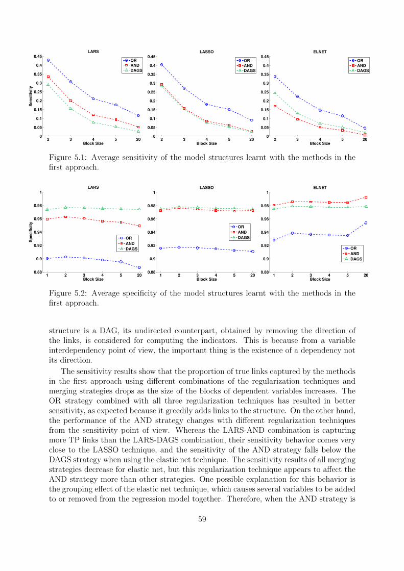
2 3 4 5 200

0.05

0.1

0.15

0.2

0.25

0.3

0.35

0.4

0.45

Block Size

Se

ns

itiv

ity

LARS

OR

AND

DAGS

2 3 4 5 200

0.05

0.1

0.15

0.2

0.25

0.3

0.35

0.4

0.45

Block SizeS

en

sit

ivit

y

LASSO

OR

AND

DAGS

2 3 4 5 200

0.05

0.1

0.15

0.2

0.25

0.3

0.35

0.4

0.45

Block Size

Se

ns

itiv

ity

ELNET

OR

AND

DAGS

Figure 5.1: Average sensitivity of the model structures learnt with the methods in thefirst approach.

1 2 3 4 5 200.88

0.9

0.92

0.94

0.96

0.98

1

Block Size

Sp

ec

ific

ity

LARS

OR

AND

DAGS

1 2 3 4 5 200.88

0.9

0.92

0.94

0.96

0.98

1

Block Size

Sp

ec

ific

ity

LASSO

OR

AND

DAGS

1 2 3 4 5 200.88

0.9

0.92

0.94

0.96

0.98

1

Block Size

Sp

ec

ific

ity

ELNET

OR

AND

DAGS

Figure 5.2: Average specificity of the model structures learnt with the methods in thefirst approach.

structure is a DAG, its undirected counterpart, obtained by removing the direction ofthe links, is considered for computing the indicators. This is because from a variableinterdependency point of view, the important thing is the existence of a dependency notits direction.

The sensitivity results show that the proportion of true links captured by the methodsin the first approach using different combinations of the regularization techniques andmerging strategies drops as the size of the blocks of dependent variables increases. TheOR strategy combined with all three regularization techniques has resulted in bettersensitivity, as expected because it greedily adds links to the structure. On the other hand,the performance of the AND strategy changes with different regularization techniquesfrom the sensitivity point of view. Whereas the LARS-AND combination is capturingmore TP links than the LARS-DAGS combination, their sensitivity behavior comes veryclose to the LASSO technique, and the sensitivity of the AND strategy falls below theDAGS strategy when using the elastic net technique. The sensitivity results of all mergingstrategies decrease for elastic net, but this regularization technique appears to affect theAND strategy more than other strategies. One possible explanation for this behavior isthe grouping effect of the elastic net technique, which causes several variables to be addedto or removed from the regression model together. Therefore, when the AND strategy is

59

2 3 4 5 200.1

0.2

0.3

0.4

0.5

0.6

0.7

0.8

0.9

Se

ns

itiv

ity

Block Size

Shrinkage

GLASSO

(a) Sensitivity

1 2 3 4 5 200.1

0.2

0.3

0.4

0.5

0.6

0.7

0.8

0.9

Sp

ec

ific

ity

Block Size

Shrinkage

GLASSO

(b) Specificity

Figure 5.3: Average accuracy of the model structures learnt in the second approach.

used to couple all regression models, a group of variables is less likely to have a mutualrelationship (as required by the AND strategy). Thus the resulting structure becomessparser and may miss many TP links.

From the specificity point of view, the results show that the tendency of regularizationtechniques to obtain sparser models causes the structures learnt by the methods in thefirst approach to include very few spurious links. Increased block sizes do not seem toconsiderably affect these methods. Note at this point that, as shown in Table 5.1, thenumber of model independencies is larger with smaller block sizes. Therefore, normallyone expects to see smaller specificity values for smaller block sizes. As block size increases,regularization techniques like LARS and LASSO tend to add more dependencies betweenthe variables. However, as we saw with the sensitivity results, many of these links areincorrect and, thus, the number of FP links increases. Another point to be considered hereis the total number of dependencies in a model compared with the sample size used forlearning. This can affect the sparsity assumption based on which the consistency of someof the regularized model estimation methods in the first approach is shown [Meinshausenand Buhlmann, 2006].

When comparing the specificity and sensitivity results of different combinations ofregularization techniques and merging strategies, they seem to be complementary. Forexample, the DAGS strategy results in poorer sensitivity results compared with the othertwo merging strategies combined with the LARS technique, but specificity is better.Whereas the sensitivity behavior of the AND strategy combined with the elastic nettechnique is worse than others, the same combination obtains better specificity resultscompared with all other combinations for all block sizes. Therefore, if a specific methodtends to add more links to the structure (like the LARS-OR combination), the probabilityof recovering TP links will clearly increase, but so will the possibility of adding FP links.On the other hand, conservative methods like the ELNET-AND combination will hitfewer TP links but also add fewer spurious links to the structure.

Figure 5.3 shows the sensitivity and specificity of the structures learnt by the methodsin the second approach. Since these methods do not explicitly obtain a structure, thestructure encoded in the covariance matrix of the estimated MGD is used to evaluate theirability to recover the true structure. This structure is obtained from the zero pattern inthe inverse covariance matrix by introducing a link between every two variables whose

60

respective entry in the inverse covariance matrix is not zero. The results show that thetwo methods in the second approach also follow a similar trend to the methods in thefirst approach: a decrease in the sensitivity and an almost uniform specificity as the sizeof the dependent variables block increases. These two methods discover more links thanthe methods in the first approach. Shrinkage estimation, especially, tends to add manylinks to the structure, and the increase in the number of dependent variables has lesseffect on this method. This results in a sensitivity of more than 50% for all block sizes.However, the specificity results show that many of the links that this method adds tothe model are spurious and this method generally tends to obtain denser structures thanother methods in either of the approaches. The graphical LASSO method behaves morelike the methods in the first approach, and especially the LARS-OR and LASSO-ORcombinations, as this method also uses a similar regularization mechanism by adding aLASSO penalization term to the ML estimation of the MGD.

5.3.2 Time Complexity

The computational time needed by an algorithm is an important feature that can affectits range of application and how it is going to be applied. In the case of EDAs, it isparticularly critical since they make intensive use of learning methods. In this section,we examine the time complexity of the methods in each of the two approaches. Themethods in the first approach have include three-step structure learning plus a parameterestimation of the target MGD. As already mentioned, the computational complexity ofcomputing the whole regularization path of a regularized regression model for a variablewith the LARS technique (which is also used as the base algorithm for the other tworegularization techniques considered here) is O(n3 +Nn2). Note that in high-dimensionalproblems, which is the case in our study, it is far less than this. The cost of selectingthe best regression solution from the regularization path is O(lN), where l is the numberof different solutions found for the regression model, and it is of order O(n). These twosteps are repeated for each of the n variables.

The AND and OR strategies used in the third step to merge the n models learntfor the variables are simple and only require O(n2) computations. However, the DAGSstrategy is usually very costly and has a computational complexity of O(kNn2 + kn4),where k is the number of iterations that it takes the local greedy algorithm to searchthe constrained space. Finally, the algorithm used to estimate the covariance matrixaccording to the structure obtained by AND and OR strategies has a cost of O(Nn2).

The shrinkage estimation and graphical LASSO methods both have a total compu-tational complexity of O(Nn2). The covariance matrix computation dominates the timerequirement of computing the mean vector of the MGD, which thus does not influencethe total cost of model estimation. The sampling algorithm used to generate M newsolutions from the estimated MGD requires O(n3 +Mn2) computations. This is also thecase for the PLS algorithm when sampling a Bayesian network.

Figures 5.4 and 5.5 show the total time that it takes all the methods in the firstapproach to learn a probabilistic model and then sample this model to generate a popu-lation of 1000 solutions, on a machine with 2.66 GHz Intel Core-i5 processor and 6 GBof memory. All the results are averaged over 30 independent runs. As expected, theDAGS strategy takes longer than the other merging strategies, though the choice of the

61

1 2 3 4 5 20

5

10

15

20

25

Block Size

Mo

de

l B

uil

din

g T

ime

(s

ec

on

ds

)

LARS

OR

AND

DAGS

1 2 3 4 5 20

5

10

15

20

25

Block SizeM

od

el B

uild

ing

Tim

e (

seco

nd

s)

LASSO

OR

AND

DAGS

1 2 3 4 5 20

5

10

15

20

25

Block Size

Mo

del B

uild

ing

Tim

e (

seco

nd

s)

ELNET

OR

AND

DAGS

Figure 5.4: Average model building time for the methods in the first approach.

1 2 3 4 5 2010

−3

10−2

10−1

100

Block Size

Mo

del S

am

plin

g T

ime (

seco

nd

s)

LARS

OR

AND

DAGS

1 2 3 4 5 2010

−3

10−2

10−1

100

Block Size

Mo

del S

am

plin

g T

ime (

seco

nd

s)

LASSO

OR

AND

DAGS

1 2 3 4 5 2010

−3

10−2

10−1

100

Block Size

Mo

del S

am

plin

g T

ime (

seco

nd

s)

ELNET

OR

AND

DAGS

Figure 5.5: Average model sampling time for the methods in the first approach.

regularization technique has a big influence on this strategy, with the LARS techniquerequiring less and elastic net technique more time. The regularization technique also hasan impact on the AND and OR strategies combined with the elastic net technique, whichtakes less time than the other two regularization techniques. This can be explained bythe sparser structures obtained by this regularization technique which in turn would leadto the estimation of fewer parameters. However, sparser structures have the oppositeeffect on the time requirement of the DAGS strategy. This can be traced back to thefact that the greedy local search algorithm is forced to reject many of the possible moveswhen searching a constrained space and it therefore takes longer to find a valid move.

The question is then whether searching in a constrained space can cause the learningtime of a Bayesian network to decrease at all. Figure 5.6 compares the model learningtime required when searching an unconstrained space and a space constrained using theLARS technique. Both methods use the same greedy local search algorithm with a BICscoring metric. Here, reference models with the increasing number of variables and equalsize of dependent variables blocks, set to 5 (quint variate model), were sampled to generatepopulations of solutions, with a fixed n/N ratio of 10. These populations were then usedfor learning Bayesian networks. The results are averaged over 30 independent runs. TheLARS-AND method is also included in the results for better comparison. We found thatwhile, the model learning time of the constrained DAGS is larger, for smaller number ofvariables the computational time required by the unconstrained DAGS grows faster as

62

100 200 300 400 500 600 700 800 900 100010

0

101

102

103

Problem SizeM

od

el

Bu

ild

ing

Tim

e (

se

co

nd

s)

LARS−DAGSearch

DAGSearch

Figure 5.6: Average model-building time for constrained and unconstrained DAG searchalgorithms on different problem sizes.

1 2 3 4 5 2010

−3

10−2

10−1

100

101

102

Block Size

Mo

del B

uild

ing

Tim

e (

seco

nd

s)

Shrinkage

GLASSO

(a) Model Building Time

1 2 3 4 5 2010

−3

10−2

10−1

100

101

102

Block Size

Mo

del S

am

plin

g T

ime (

seco

nd

s)

Shrinkage

GLASSO

(b) Model Sampling Time

Figure 5.7: Average model-building (left) and sampling (right) time for the methods inthe second approach.

the number of variables increase and becomes considerably larger than its constrainedcounterpart. This is because for larger number of variables, the search space becomes sohuge that any kind of space-constraining information can serve as a heuristic to improvethe search. For the difference in the estimation accuracy of these two methods, see[Schmidt et al., 2007; Vidaurre et al., 2010].

As the model sampling times show (Figure 5.5), it takes longer to generate newsolutions from a Bayesian network using the PLS algorithm than the algorithm used tosample an MGD. Although the same algorithm is used to sample the models learnt bythe AND and OR strategies, the results show that the estimated models can affect thesampling time depending on the regularization technique and the block size. Generally,however both the model learning and sampling times do not appear to change considerablyby increasing the size of dependent variables block, since all these models have the samedimension. Figure 5.6 shows, on the other hand, that the increase in the number ofvariables raises the algorithm time requirement, as expected from the computationalcomplexity analysis.

Figure 5.7 shows the average model-learning and sampling times for the two meth-ods in the second approach, on the same machine. Sampling times are computed forgenerating a population of 1000 solutions from the learnt model. The graphical LASSOmethod takes significantly longer to estimate the model than shrinkage estimation, and

63

1 2 3 4 5 20

3.5

4

4.5

5

5.5x 10

5

Block Size

Neg

ati

ve L

og

−L

ikelih

oo

d

LARS

OR

AND

DAGS

1 2 3 4 5 20

3.5

4

4.5

5

5.5x 10

5

Block SizeN

eg

ati

ve

Lo

g−

Lik

eli

ho

od

LASSO

OR

AND

DAGS

1 2 3 4 5 20

3.5

4

4.5

5

5.5x 10

5

Block Size

Ne

ga

tiv

e L

og

−L

ike

lih

oo

d

ELNET

OR

AND

DAGS

Figure 5.8: Average negative log-likelihood of the reference Gaussian distributions ob-tained for model estimation methods in the first approach.

its time requirements closely follow those of the methods in the first approach, especiallythe LARS-OR and LASSO-OR combinations (whose structural accuracy is similar, too).Again, the size of blocks of dependent variables does not have a substantial effect onthe computational time of these two methods, although further experiments have shownthat graphical LASSO is highly sensitive to the violation of the conditions in the sparsityassumption. Section 5.3.4 discusses this issue in more detail. The time requirements ofthe shrinkage estimation method make it a perfect candidate for use within more complexalgorithms like EDAs that require very fast-performing components.

5.3.3 Likelihood Function

Estimating an accurate structure is an important feature of a probabilistic model estima-tion method. For the purpose of model estimation and sampling in EDAs (Algorithm 2.1),however, it is more important to be able to generate solutions that are very close to thereal problem solution, which is assumed to be representable with a probability distribu-tion. One way to investigate this closeness is to compare the model estimated in EDA withthe actual probabilistic model underlying the problem. Measures like Kullback-Leiblerdivergence [Kullback and Leibler, 1951] or Hellinger distance [Le Cam and Lo Yang,2000] can be used for this purpose. Another possibility is to evaluate the overall modelestimation and sampling of EDAs in order to also take into account the inevitable modelsampling error that is present in practice. This is also closer to the actual procedureenacted in each generation of an EDA. The evaluation measure computed in this study isthe negative log-likelihood (NLL) of the reference Gaussian models (see Table 5.1) giventhe population of solutions generated from the estimated models.

Figure 5.8 shows the NLL values of the reference Gaussian models with different blocksizes, computed from the populations generated using the models learnt with the methodsin the first approach. Each of the generated populations had a size of 1000. For thefirst two regularization techniques, the NLL values obtained with the DAGS strategy onlarger block sizes tend to infinity and are therefore not included in the figures. Mergingstrategies are ordered similarly for all regularization techniques, with the NLL of ORstrategy turned out to be better and DAGS worse. This is consistent with the structuralaccuracy results and reveals the mixed effect of sensitivity and specificity analysis for the

64

1 2 3 4 5 203.2

3.4

3.6

3.8

4

4.2

4.4

4.6

4.8

5x 10

5

Block SizeN

eg

ati

ve

Lo

g−

Lik

eli

ho

od

Shrinkage

GLASSO

Figure 5.9: Average negative log-likelihood of the reference Gaussian distributions ob-tained for the estimation methods in the second approach.

methods in the first approach. The NLLs computed for these methods grow visibly asblock size increases, suggesting that as the number of dependent variables in the problemincreases the estimated models and populations generated from these models move fartherfrom the reference models, from a log-likelihood point of view.

Figure 5.9 shows the NLL results for the two methods in the second approach, wheregraphical LASSO results in better NLL values than the shrinkage method. Shrinkageestimation is able to capture more dependencies, but, at the same time, it adds manyspurious links to the structure. As a result, the estimated probability distribution gener-ates solutions that are less likely producible by the reference models. From the NLL valuesfor graphical LASSO, and for LARS-OR and LASSO-OR used in the first approach, wealso find that these methods behave similarly. Also, the NLL values computed for graph-ical LASSO and for the ML estimation of the MGD are almost equal, showing that, froma log-likelihood point of view, the addition of a LASSO penalization term does not havemuch impact on the probability estimation of the graphical LASSO method.

5.3.4 Regularization Parameter in Graphical LASSO Method

The regularization techniques employed in the first approach output the whole regular-ization path for varying values of the regularization parameter (λ) and then select theparameter resulting in the best regression solution according to a model selection metric.Also, the value of the shrinkage intensity in the shrinkage estimation method is analyti-cally computed according to the learning data set. However, the regularization parameterof the graphical LASSO method is left open, as it is not practicable to compute the wholeregularization path for this method, especially for high-dimensional problems.

To examine the influence of the regularization parameter, we apply the graphicalLASSO method with different values of this parameter for model estimation. The modellearning times and the corresponding NLL values computed for this method are shownin Figure 5.10. Models are estimated from populations with increasing sizes, generatedfrom the bivariate reference model by decreasing the n/N ratio from 10 to 0.2 (graduallygetting away from high-dimensionality) in order to also investigate the effect of populationsize on this method. NLL values are computed using populations of size 1000 generatedfrom the estimated models. All of the results are averaged over 30 independent runs.

65

10 20 50 100 200 500

10−1

100

101

Population Size

Mo

del B

uild

ing

Tim

e (

seco

nd

s)

λ=0.01

λ=0.1

λ=1

λ=5

(a) Model Building Time

10 20 50 100 200 5003.3

3.35

3.4

3.45

3.5

3.55

3.6

3.65

3.7x 10

5

Population Size

Neg

ati

ve L

og

Lik

elih

oo

d

λ=0.01

λ=0.1

λ=1

λ=5

(b) Negative Log-Likelihood

Figure 5.10: Average model-building time (left) and negative log-likelihood of the bivari-ate Gaussian distribution (right) obtained for the graphical LASSO method with differentregularization parameter (λ) values.

Clearly, whereas model estimation is faster with larger values of the regularizationparameter, the solutions generated from these models are less likely from the referencemodel point of view. On the other hand, small values of this parameter (close to zero)will result in better NLL values, though at a higher computational cost. This observationsuggests that, as reported in a previous study [Karshenas et al., 2011a], the choice of avalue for the regularization parameter of this method call for a trade-off between howgood an estimation is and the time required to estimate the model.

The model learning times also show that, as population size grows the time requiredby the graphical LASSO method with a specific value of the regularization parametergradually decreases. This is why it is expected to be more costly to estimate a model,with a specific dimension and block size, from populations with larger sizes. One possibleexplanation for this behavior is that with larger populations that better fulfill the spar-sity assumption [Meinshausen and Buhlmann, 2006], more harmonious statistics can becollected from the population, allowing the method to converge faster. However, as thecomputed NLL values show, the population size increase does not affect the probabilityof the generated solutions from the reference model point of view. Based on these re-sults, a 0.1 value is used for the regularization parameter of the graphical LASSO methodthroughout the thesis.

5.4 Conclusions

The use of regularized model estimation in EDAs for continuous optimization was pro-posed and studied in this chapter. It was argued that the use of regularization techniquescan lead to a more robust model estimation in EDAs. This improves performance inhigh-dimensional settings, while keeping the population size and therefore the number offunction evaluations relatively low.

Considering a high-dimensional setting, different methods for regularized estimationof Gaussian distributions in two general approaches were analyzed from several pointsof view: true structure recovery, time complexity, and likelihood. The analysis resultsshowed the properties of these methods, like their tendency in including dependencies

66

between variables and the learning/sampling times as the number of variables and theirinteractions increase. It was observed that an important factor affecting regularized modelestimation is the level of variable dependencies in the problem.

67

68

Chapter 6

Regularization-Based EDA inContinuous Optimization

6.1 Introduction

Given a fitness or objective function f : D 7→ R, the goal of (single-objective) optimizationis to find solution(s) x∗ such that (assuming smaller values of f are preferred)

x∗ = arg minx∈D

f(x) (6.1)

If the optimization algorithm does not use any problem-specific information for findingthe optimal solution(s), it is called a black-box or general-purpose optimization algorithm.In continuous domains, we have D ⊆ Rn, where n is the dimension of the input domain.Since this set is uncountable, in general it is not possible to find an upper bound on thenumber of steps required to reach the optimal solution(s) to a continuous optimizationfunction. Therefore, in this case the algorithms that can get closer to the optimal solutionsfaster (e.g. in smaller number of steps) are favorable.

In the last chapter, we saw how regularization techniques can be used for modelestimation in EDAs. The analysis especially considered high-dimensional settings tostudy the performance of regularized model learning from small populations with respectto several criteria. In this chapter we analyze this type of model learning from thecontinuous function optimization point of view and compare its performance with severalother well-known continuous EDAs. This work is published in [Karshenas et al., 2013b].

6.2 RegEDA: Regularization-based EDA

The results of the regularized model estimation analysis can be used as a guideline foremploying these methods in EDAs. The regularization-based EDA (RegEDA) proposedin this chapter utilizes the regularized model estimation methods in the course of opti-mization, trying to obtain a better estimation of the distribution of the problem solutions,in order to improve performance.

The constraints on time and computational resources restrict the number of differ-ent regularized estimation methods that can be tested and compared. Therefore, forthe experiments in the rest of the chapter, some of the discussed methods were selected

69

for use in RegEDA. We selected the LARS-OR and LARS-AND methods from the firstapproach. They appear to offer a better compromise between the computational timerequirements and the quality of the estimated models, from both the structural accu-racy and NLL points of view. The resulting algorithms are called “RegEDA-LARS-OR”and “RegEDA-LARS-AND”, respectively. From the second approach, both the shrink-age estimation and graphical LASSO methods were selected and respectively used in“RegEDA-Shr” and “RegEDA-GL” algorithms. The properties of both methods moti-vate further investigation regarding optimization. In the rest of this chapter, we studythe performance of these four versions of RegEDA in function optimization.

6.3 Experiments

The proposed RegEDAs are applied for continuous function optimization in order toinvestigate how regularized model estimation affects the optimization behavior and per-formance of EDAs when applied in a high-dimensional setting. The optimization resultsof the four versions of RegEDA are compared against another four Gaussian distribution-based EDAs, which are: i) Continuous UMDA [Larranaga et al., 2000a], ii) EGNA[Larranaga et al., 2000a], iii) EMNA [Larranaga and Lozano, 2001], and iv) CMA-ES[Hansen, 2006]. All of the algorithms are implemented in Matlab R©. Specifically, we haveused Mateda-2.0 package1 [Santana et al., 2010a], which provides the implementation ofUMDA and EMNA, as the basis of our implementation framework. For the implementa-tion of LARS technique in RegEDA-LARS-OR and RegEDA-LARS-AND algorithms, wehave used the code provided by K. Sjostrand2, and the covariance shrinkage method isimplemented with the code provided by K. Murphy3. The implementation of the graph-ical LASSO is adapted for Matlab4 from the original code provided for the algorithm[Friedman et al., 2008].

For the implementation of EGNA and especially its GBN learning, we have used thecode provided by M. Schmidt and K. Murphy5 [Schmidt et al., 2007]. It slightly differsfrom the method described in Section 1.3.3 by allowing the greedy method to restartthe structure search from a new random structure after reaching a local optimum of thescore function, up to a maximum number of node score evaluations. At the end, thehighest scoring BN in all these sub-searches is returned. Since the PLS algorithm isused to sample the estimated GBN, the algorithm is referred to as “EGNA-PLS” in thepresented results. Finally, we have used the Matlab implementation of CMA-ES providedby N. Hansen6.

6.3.1 Optimization Functions

The continuous optimization functions used for the experiments are listed in Table 6.1.These optimization functions, defined on n input variables, have different properties that

1http://www.sc.ehu.es/ccwbayes/members/rsantana/software/matlab/MATEDA.html2http://www2.imm.dtu.dk/pubdb/views/edoc_download.php/3897/zip/imm3897.zip3http://www.uni-leipzig.de/~strimmer/lab/software/m-files/covshrink-kpm.zip4http://cig.fi.upm.es/components/com_phocadownload/container/GraphicalLasso.zip5http://www.cs.ubc.ca/~murphyk/Software/DAGlearn/DAGLearn.zip6http://www.lri.fr/~hansen/cmaes_inmatlab.html

70

allow to examine the performance of the tested optimization algorithms, in the presenceof different problem features. The 2D fitness landscape of some of these functions, isshown in Figure 6.1. The definitions of the functions are as follows.

• Sphere

f(x) =n∑i=1

x2i .

• Ackley

f(x) = −a exp

−b√√√√ 1

n

n∑i=1

x2i

− exp

(1

n

n∑i=1

cos(cxi)

)+ a+ e,

where a, b and c are the parameters of the function and are set to 20, 0.2 and 2π,respectively. e is Euler’s number.

• Tablet

f(x) = 106x21 +

n∑i=2

x2i .

• Cigar-Tablet

f(x) = x21 + 104

n−1∑i=2

x2i + 108x2

n.

• Michalewicz

f(x) = −n∑i=1

sin(xi) sin2m

(ix2i

π

),

where m is the parameter of the function and is set to 10. The optimum value ofthe function is different for different numbers of variables.

• Sum Cancellation

f(x) =

(10−5 +

n∑i=1

∣∣∣∣∣i∑

j=1

xj

∣∣∣∣∣)−1

.

The Sphere function is a simple optimization problem without any interdependencybetween variables. Following the smooth downhill path will lead an optimization al-gorithm to the optimal solution of the function. The Ackley function has a ruggedlandscape, although some local regions of the search space can provide information aboutthe global structure of the problem. The first variable of the Tablet function is scaledcausing the optimization algorithms to be more sensitive to changes of this variable, andtherefore the promising values of other variables may not be properly encoded in EDAmodel estimation. The Cigar-Tablet function extends the Tablet function by introducingthree different levels of scalings for the variables. The Michalewicz function does not havea proper global structure and requires more exploration for detecting promising basinsof attraction. The Sum Cancellation function is very similar to a problem called nee-dle in the haystack, especially for larger dimensions, and the function is not separable.Therefore, a very small search space is considered for this function.

71

Table 6.1: The optimization functions used in the experiments, their optimum solution(x∗) and optimum function value (f ∗). The number of variables is denoted with n.

Name Type Domain x∗ f ∗

1 Sphere min [−5, 5]n 0 02 Ackley min [−32, 32]n 0 03 Tablet min [−7.5, 7.5]n 0 04 Cigar-Tablet min [−7.5, 7.5]n 0 05 Michalewicz min [0, π]n –a –a

6 Sum Cancellation max [−0.16, 0.16]n 0 105

a Depends on n.

−5

0

5

−5

0

50

20

40

60

(a) Sphere

−5

0

5

−5

0

50

5

10

15

(b) Ackley

0

2

4

0

2

4

−2

−1

0

(c) Michalewicz

−0.2

0

0.2

−0.2

0

0.20

5

10

x 104

(d) Sum Cancellation

Figure 6.1: Fitness landscape of some of the optimization functions in two dimensions.

6.3.2 Experimental Design

Five different dimensions are tested for each of the functions: 10, 20, 50, 100 and 200variables. Population size is set to N = 10 ln(n) for all of the algorithms in an at-tempt to emulate high-dimensional settings as the number of variables increase, startingwith a certain number of solutions. For each algorithm-function-dimension combination,20 independent runs are performed. The initial population is randomly generated us-

72

10−5

10−4

10−3

10−2

10−1

100

UMDA

EMNA

EGNA−PLS

RegEDA−Shr

RegEDA−GL

RegEDA−LARS−AND

RegEDA−LARS−OR

Time (seconds)

Selection

Replacement

Model Learning

Model Sampling

Figure 6.2: Average time requirements for the main steps of RegEDAs and their compar-ison with other EDAs. The number of variables is 50.

ing a uniform distribution over the domain of variables. All algorithms terminate whenthe maximum number of generations, set to 500, is reached. Apart from this stoppingcriterion, when an algorithm gets stuck in a stalemate situation for 100 consecutive gen-erations, it stops so as not to waste computational time. A stalemate situation is verifiedif the improvement in the fitness function is less than 10−8. Figure 6.2 gives an insightinto the computational time requirements of the main steps of RegEDAs, which are com-pared with three other Gaussian-based EDAs used in the experiments of this section.The presented results are obtained on a machine with 2.66 GHz Intel Core-i5 processorand 6 GB of memory, and are averaged over 500 generations of a run.

For all EDAs, solutions are selected using truncation selection with a τ = 0.5 thresh-old. Except for CMA-ES, which completely replaces the population in each generationwith new solutions, all other algorithms generate N/2 new offspring solutions in thesampling step. The newly generated solutions are repaired using a simple repairmentstrategy, where unacceptable values are replaced by a new value randomly chosen fromthe domain of the corresponding variable. An elitist replacement strategy is used to in-corporate the offspring solutions into the population, where the best N solutions fromthe combination of offspring solutions and solutions in the population are selected toform the next-generation population. The initial standard deviation of CMA-ES (oneof algorithm’s input parameters) is set to one third of each variable’s domain, as it issuggested in [Hansen, 2006]. This algorithm is considered to be in a stalemate situationif the improvement in the fitness function is less than 10−12 (which is less strict thanother algorithms).

6.3.3 Results

Figures 6.3–6.8 show the average best achieved values (BAVs) along the evolution path ofRegEDAs and the other four EDAs, applied to the optimization functions. The presentedresults are averaged over the 20 runs performed. For runs that an algorithm terminatesbefore reaching the maximum number of generations, the rest of evolution path is paddedwith the BAV of the last executed generation. For some of the functions, the BAVs aredepicted on a logarithmic scale so as to better discriminate algorithms’ performance.

The results for all functions show that, when considering the distance between BAVs

73

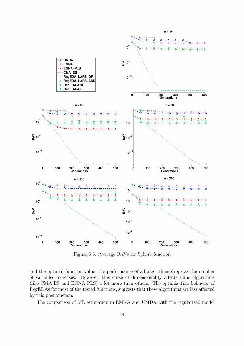
0 2 4 6 8 100

0.2

0.4

0.6

0.8

1

UMDA

EMNA

EGNA−PLS

CMA−ES

RegEDA−LARS−OR

RegEDA−LARS−AND

RegEDA−Shr

RegEDA−GL

0 100 200 300 400 500

10−10

10−5

100

BA

V

Generations

n = 10

0 100 200 300 400 500

10−10

10−5

100

BA

V

Generations

n = 20

0 100 200 300 400 500

10−10

10−5

100

BA

V

Generations

n = 50

0 100 200 300 400 500

10−10

10−5

100

105

BA

V

Generations

n = 100

0 100 200 300 400 500

10−4

10−2

100

102

104

BA

V

Generations

n = 200

Figure 6.3: Average BAVs for Sphere function

and the optimal function value, the performance of all algorithms drops as the numberof variables increases. However, this curse of dimensionality affects some algorithms(like CMA-ES and EGNA-PLS) a lot more than others. The optimization behavior ofRegEDAs for most of the tested functions, suggests that these algorithms are less affectedby this phenomenon.

The comparison of ML estimation in EMNA and UMDA with the regularized model

74

0 2 4 6 8 100

0.2

0.4

0.6

0.8

1

UMDA

EMNA

EGNA−PLS

CMA−ES

RegEDA−LARS−OR

RegEDA−LARS−AND

RegEDA−Shr

RegEDA−GL

0 100 200 300 400 500

5

10

15

20

BA

V

Generations

n = 10

0 100 200 300 400 500

5

10

15

20

BA

V

Generations

n = 20

0 100 200 300 400 500

2

4

6

8

10

12

14

16

18

20

BA

V

Generations

n = 50

0 100 200 300 400 500

2

4

6

8

10

12

14

16

18

20

BA

V

Generations

n = 100

0 100 200 300 400 500

4

6

8

10

12

14

16

18

20

BA

V

Generations

n = 200

Figure 6.4: Average BAVs for Ackley function

estimation in RegEDAs better illustrates the difference in the performance of RegEDAsand how they are affected by the increases in the problem size. Since all other parts of thetested algorithms are the same (except for CMA-ES), the similarities and differences in theoptimization performance of these algorithms can be attributed to the model estimationmethods that they employ. For example, the performance of RegEDA-Shr and UMDA is

75

0 2 4 6 8 100

0.2

0.4

0.6

0.8

1

UMDA

EMNA

EGNA−PLS

CMA−ES

RegEDA−LARS−OR

RegEDA−LARS−AND

RegEDA−Shr

RegEDA−GL

0 100 200 300 400 50010

−15

10−10

10−5

100

105

BA

V

Generations

n = 10

0 100 200 300 400 50010

−6

10−4

10−2

100

102

104

106

BA

V

Generations

n = 20

0 100 200 300 400 500

100

101

102

103

104

105

106

107

BA

V

Generations

n = 50

0 100 200 300 400 500

100

101

102

103

104

105

106

107

BA

V

Generations

n = 100

0 100 200 300 400 500

101

102

103

104

105

106

107

BA

V

Generations

n = 200

Figure 6.5: Average BAVs for Tablet function

very close for most of the functions, suggesting that the shrinkage estimation method isshrinking most of the off-diagonal entries in the covariance matrix to close-to-zero values.This property is especially useful when dealing with separable optimization problems.A comparison of the performances of RegEDA-Shr, and UMDA and EMNA for Spherefunctions (Figure 6.3), clearly shows that the model estimation employed in RegEDA-Shris more efficient, since it leads to a regularized combination of the models used in EMNA

76

0 2 4 6 8 100

0.2

0.4

0.6

0.8

1

UMDA

EMNA

EGNA−PLS

CMA−ES

RegEDA−LARS−OR

RegEDA−LARS−AND

RegEDA−Shr

RegEDA−GL

0 100 200 300 400 50010

−15

10−10

10−5

100

105

BA

V

Generations

n = 10

0 100 200 300 400 50010

−5

100

105

BA

V

Generations

n = 20

0 100 200 300 400 50010

3

104

105

106

107

108

109

BA

V

Generations

n = 50

0 100 200 300 400 500

104

105

106

107

108

109

BA

V

Generations

n = 100

0 100 200 300 400 500

105

106

107

108

109

BA

V

Generations

n = 200

Figure 6.6: Average BAVs for Cigar-Tablet function

and UMDA.

The conservative merging strategy used in RegEDA-LARS-AND model estimationcauses fewer dependencies to be added to the model, leading to sparser structures. Thefact that, for many of the functions, this algorithm behaves similarly to UMDA, andtherefore RegEDA-Shr, shows that the sparsity pattern of these structures is very similarto diagonal matrices in the presence of problem separability. When the problem is not

77

0 2 4 6 8 100

0.2

0.4

0.6

0.8

1

UMDA

EMNA

EGNA−PLS

CMA−ES

RegEDA−LARS−OR

RegEDA−LARS−AND

RegEDA−Shr

RegEDA−GL

0 100 200 300 400 500

−9

−8

−7

−6

−5

−4

−3

−2

−1

BA

V

Generations

n = 10

0 100 200 300 400 500

−16

−14

−12

−10

−8

−6

−4

−2

BA

V

Generations

n = 20

0 100 200 300 400 500

−30

−25

−20

−15

−10

−5

BA

V

Generations

n = 50

0 100 200 300 400 500−30

−28

−26

−24

−22

−20

−18

−16

−14

−12

−10

BA

V

Generations

n = 100

0 100 200 300 400 500

−50

−45

−40

−35

−30

−25

−20

BA

V

Generations

n = 200

Figure 6.7: Average BAVs for Michalewicz function

separable (like the Sum Cancellation function – Figure 6.8), RegEDA-LARS-AND can,thanks to this regularized model estimation method, perform a more concentrated searchby including only what are, according to the regularization technique, the more importantlinks. Therefore this algorithm is able to outperform other algorithms with the increasein problem dimensionality.

78

0 2 4 6 8 100

0.2

0.4

0.6

0.8

1

UMDA

EMNA

EGNA−PLS

CMA−ES

RegEDA−LARS−OR

RegEDA−LARS−AND

RegEDA−Shr

RegEDA−GL

0 100 200 300 400 500

100

101

102

103

104

105

BA

V

Generations

n = 10

0 100 200 300 400 500

100

101

102

103

104

BA

V

Generations

n = 20

0 100 200 300 400 500

10−1

100

BA

V

Generations

n = 50

0 100 200 300 400 500

10−1

100

BA

V

Generations

n = 100

0 100 200 300 400 500

10−2

10−1

BA

V

Generations

n = 200

Figure 6.8: Average BAVs for Sum Cancellation function

The optimization performance of RegEDA-GL compared with EMNA is especiallyinteresting in these experiments. The model estimation method in the two algorithmsdiffers only as to the regularization term added to ML estimation of MGD in the graph-ical LASSO method (see Section 4.3). The results show that, for some of the functions(like Sphere and Ackley – Figures 6.3 and 6.4), regularization improves the average per-formance of RegEDA-GL while, for some others (Michalewicz and Sum Cancellation –

79

Figures 6.7 and 6.8), this algorithm is not able to obtain good BAVs as EMNA. Con-sidering the properties of these functions, it appears that the use of regularization willresult in better model estimation if the problem has a global structure, whereas lackof such information has a negative effect on the regularized model estimation used inRegEDA-GL.

The similar optimization behavior of RegEDA-LARS-OR and EMNA for many ofthe functions suggests that the MGDs estimated with the greedy merging strategy em-ployed in RegEDA-LARS-OR are very similar to those obtained by ML estimation. Forexample, a good option, in the absence of useful properties in some of the functions(like Michalewicz – Figure 6.7), for use by the optimization algorithm, could be a coarseestimation of the search space. Model estimation in RegEDA-LARS-OR simulates thiscoarse estimation by adding many links to the structure considering all possible variabledependencies. However, the use of regularization to detect the dependencies, in the pres-ence of specific problem properties (like separability) causes the algorithm to perform afiner search.

6.3.4 Discussion

There are some common points concerning the performance of the algorithms on thetested functions. First, most of the algorithms show a different optimization behaviorfrom one function to another depending on the different features of these functions.This suggests that although no explicit rotation and translation is applied, the set ofselected functions form a good benchmark for the experiments. On the other hand, theGaussian distribution-based model estimation used in the algorithms is invariant to thesetransformations (except UMDA). Second, the performance of all the algorithms is affectedby the increase in the number of variables, from the viewpoint of the distance betweenBAVs and optimal function value. Some of the algorithms, like CMA-ES, appear to beable to improve their BAVs if given more time, but it is evident from the results that theirperformance is influenced considerably more than the RegEDAs proposed here, when thenumber of variables increase.

Thirdly, the population size of all algorithms is equally set to be of a logarithmicorder of the problem size, resembling a high-dimensional setting. Thus, for most ofthe functions and especially larger dimensions, almost all the algorithms get stuck in astalemate situation in the early generations of the search. For the purpose of studying theeffect of regularized model estimation, none of the algorithms (except CMA-ES, whichuses specific variance scaling techniques) use any kind of explicit diversity preservationtechniques. The fact that all other parts of the algorithms are the same is helpful forgaining a better understanding of how different model estimation methods affect theoptimization behavior.

Table 6.2 shows the statistical analysis results for the BAVs obtained by the algorithmson each dimension of each function. The non-parametric Friedman rank test [Derrac et al.,2011] is used to check for the statistical difference in algorithm’s performance. The nullhypothesis that all the algorithms have an equal average rank is rejected with a p-valueless than 10−8 for all functions and all dimensions. The values shown in each entry ofTable 6.2 are the final average BAVs obtained by the algorithm in the column, appliedon the function-dimension combination in the row. The numbers in parentheses show

80

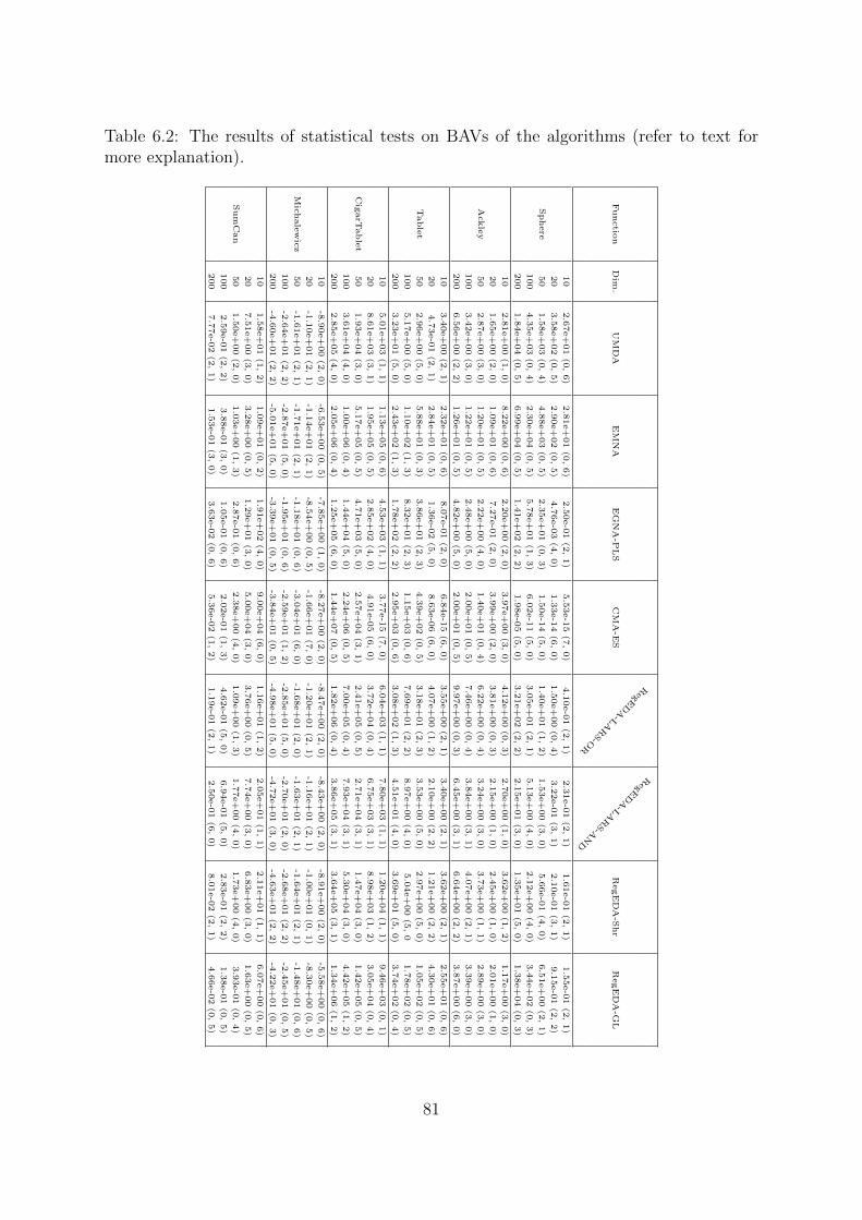
Table 6.2: The results of statistical tests on BAVs of the algorithms (refer to text formore explanation).

Functio

nD

im.

UM

DA

EM

NA

EG

NA

-PL

SC

MA

-ES

RegE

DA

-LA

RS-O

R

RegE

DA

-LA

RS-A

ND

RegE

DA

-Shr

RegE

DA

-GL

Sphere

10

2.6

7e+

01

(0,

6)

2.8

1e+

01

(0,

6)

2.5

0e-0

1(2

,1)

5.5

3e-1

5(7

,0)

4.1

0e-0

1(2

,1)

2.3

1e-0

1(2

,1)

1.6

1e-0

1(2

,1)

1.5

5e-0

1(2

,1)

20

3.5

8e+

02

(0,

5)

2.9

0e+

02

(0,

5)

4.7

6e-0

3(4

,0)

1.3

3e-1

4(6

,0)

1.5

0e+

00

(0,

4)

3.2

2e-0

1(3

,1)

2.1

0e-0

1(3

,1)

9.1

5e-0

1(2

,2)

50

1.5

8e+

03

(0,

4)

4.8

8e+

03

(0,

5)

2.3

5e+

01

(0,

3)

1.5

0e-1

4(5

,0)

1.4

0e+

01

(1,

2)

1.5

3e+

00

(3,

0)

5.6

6e-0

1(4

,0)

6.5

1e+

00

(2,

1)

100

4.3

5e+

03

(0,

4)

2.3

0e+

04

(0,

5)

5.7

8e+

01

(1,

3)

6.0

2e-1

1(5

,0)

3.0

5e+

01

(2,

1)

5.1

3e+

00

(4,

0)

2.1

2e+

00

(4,

0)

3.4

4e+

02

(0,

3)

200

1.8

4e+

04

(0,

5)

6.9

9e+

04

(0,

5)

1.4

1e+

02

(2,

2)

1.9

8e-0

5(5

,0)

3.2

1e+

02

(2,

2)

2.1

5e+

01

(3,

0)

1.3

5e+

01

(5,

0)

1.3

8e+

04

(0,

3)

Ackle

y

10

2.8

1e+

00

(1,

0)

8.2

2e+

00

(0,

6)

2.2

0e+

00

(2,

0)

3.9

7e+

00

(3,

0)

4.1

2e+

00

(0,

3)

2.7

0e+

00

(1,

0)

3.6

2e+

00

(1,

2)

1.1

7e+

00

(3,

0)

20

1.6

5e+

00

(2,

0)

1.0

9e+

01

(0,

6)

7.2

7e-0

1(2

,0)

3.9

9e+

00

(2,

0)

3.8

1e+

00

(0,

3)

2.1

5e+

00

(1,

0)

2.4

5e+

00

(1,

0)

2.0

1e+

00

(1,

0)

50

2.8

7e+

00

(3,

0)

1.2

0e+

01

(0,

5)

2.2

2e+

00

(4,

0)

1.4

0e+

01

(0,

4)

6.2

2e+

00

(0,

4)

3.2

4e+

00

(3,

0)

3.7

3e+

00

(1,

1)

2.8

9e+

00

(3,

0)

100

3.4

2e+

00

(3,

0)

1.2

2e+

01

(0,

5)

2.4

8e+

00

(5,

0)

2.0

0e+

01

(0,

5)

7.4

6e+

00

(0,

4)

3.8

4e+

00

(3,

1)

4.0

7e+

00

(2,

1)

3.3

9e+

00

(3,

0)

200

6.5

6e+

00

(2,

2)

1.2

6e+

01

(0,

5)

4.8

2e+

00

(5,

0)

2.0

0e+

01

(0,

5)

9.9

7e+

00

(0,

3)

6.4

5e+

00

(3,

1)

6.6

4e+

00

(2,

2)

3.8

7e+

00

(6,

0)

Table

t

10

3.4

0e+

00

(2,

1)

2.3

2e+

01

(0,

6)

8.0

7e-0

1(2

,0)

6.8

4e-1

5(6

,0)

3.5

5e+

00

(2,

1)

3.4

0e+

00

(2,

1)

3.6

2e+

00

(2,

1)

2.5

5e+

01

(0,

6)

20

4.7

3e-0

1(2

,1)

2.8

4e+

01

(0,

5)

1.3

6e-0

2(5

,0)

8.6

3e-0

6(6

,0)

4.0

7e+

00

(1,

2)

2.1

0e+

00

(2,

2)

1.2

1e+

00

(2,

2)

4.3

0e+

01

(0,

6)

50

2.9

6e+

00

(5,

0)

5.8

8e+

01

(0,

3)

3.8

6e+

01

(2,

3)

4.3

9e+

02

(0,

5)

3.1

8e+

01

(2,

3)

3.5

3e+

00

(5,

0)

2.9

7e+

00

(5,

0)

1.0

5e+

02

(0,

5)

100

5.1

7e+

00

(5,

0)

1.1

0e+

02

(1,

3)

8.3

2e+

01

(2,

3)

1.1

5e+

03

(0,

6)

7.6

9e+

01

(2,

2)

8.9

7e+

00

(4,

0)

5.0

4e+

00

(5,

01.7

8e+

02

(0,

5)

200

3.2

3e+

01

(5,

0)

2.4

3e+

02

(1,

3)

1.7

8e+

02

(2,

2)

2.9

5e+

03

(0,

6)

3.0

8e+

02

(1,

3)

4.5

1e+

01

(4,

0)

3.6

9e+

01

(5,

0)

3.7

4e+

02

(0,

4)

Cig

arT

able

t

10

5.0

1e+

03

(1,

1)

1.1

3e+

05

(0,

6)

4.5

3e+

03

(1,

1)

3.7

7e-1

5(7

,0)

6.0

4e+

03

(1,

1)

7.8

0e+

03

(1,

1)

1.2

0e+

04

(1,

1)

9.4

6e+

03

(0,

1)

20

8.6

1e+

03

(3,

1)

1.9

5e+

05

(0,

5)

2.8

5e+

02

(4,

0)

4.9

1e-0

5(6

,0)

3.7

2e+

04

(0,

4)

6.7

5e+

03

(3,

1)

8.9

8e+

03

(1,

2)

3.0

5e+

04

(0,

4)

50

1.9

3e+

04

(3,

0)

5.1

7e+

05

(0,

5)

4.7

1e+

03

(5,

0)

2.5

7e+

04

(3,

1)

2.4

1e+

05

(0,

5)

2.7

1e+

04

(3,

1)

1.4

7e+

04

(3,

0)

1.4

2e+

05

(0,

5)

100

3.6

1e+

04

(4,

0)

1.0

0e+

06

(0,

4)

1.4

4e+

04

(5,

0)

2.2

4e+

06

(0,

5)

7.0

0e+

05

(0,

4)

7.9

3e+

04

(3,

1)

5.3

0e+

04

(3,

0)

4.4

2e+

05

(1,

2)

200

2.8

5e+

05

(4,

0)

2.0

5e+

06

(0,

4)

1.2

5e+

05

(6,

0)

1.4

4e+

07

(0,

5)

1.8

2e+

06

(0,

4)

3.8

6e+

05

(3,

1)

3.6

4e+

05

(3,

1)

1.3

4e+

06

(1,

2)

Mic

hale

wic

z

10

-8.9

0e+

00

(2,

0)

-6.5

3e+

00

(0,

5)

-7.8

5e+

00

(1,

0)

-8.2

7e+

00

(2,

0)

-8.4

7e+

00

(2,

0)

-8.4

3e+

00

(2,

0)

-8.9

1e+

00

(2,

0)

-5.5

8e+

00

(0,

6)

20

-1.1

0e+

01

(2,

1)

-1.1

4e+

01

(2,

1)

-8.5

4e+

00

(0,

5)

-1.6

6e+

01

(7,

0)

-1.2

0e+

01

(2,

1)

-1.1

6e+

01

(2,

1)

-1.0

0e+

01

(0,

1)

-8.3

0e+

00

(0,

5)

50

-1.6

1e+

01

(2,

1)

-1.7

1e+

01

(2,

1)

-1.1

8e+

01

(0,

6)

-3.0

4e+

01

(6,

0)

-1.6

8e+

01

(2,

0)

-1.6

3e+

01

(2,

1)

-1.6

4e+

01

(2,

1)

-1.4

8e+

01

(0,

6)

100

-2.6

4e+

01

(2,

2)

-2.8

7e+

01

(5,

0)

-1.9

5e+

01

(0,

6)

-2.5

9e+

01

(1,

2)

-2.8

5e+

01

(5,

0)

-2.7

0e+

01

(2,

0)

-2.6

8e+

01

(2,

2)

-2.4

5e+

01

(0,

5)

200

-4.6

0e+

01

(2,

2)

-5.0

1e+

01

(5,

0)

-3.3

9e+

01

(0,

5)

-3.8

4e+

01

(0,

5)

-4.9

8e+

01

(5,

0)

-4.7

2e+

01

(3,

0)

-4.6

3e+

01

(2,

2)

-4.2

2e+

01

(0,

3)

Sum

Can

10

1.5

8e+

01

(1,

2)

1.0

9e+

01

(0,

2)

1.9

1e+

02

(4,

0)

9.0

0e+

04

(6,

0)

1.1

6e+

01

(1,

2)

2.0

5e+

01

(1,

1)

2.1

1e+

01

(1,

1)

6.0

7e+

00

(0,

6)

20

7.5

1e+

00

(3,

0)

3.2

8e+

00

(0,

5)

1.2

9e+

01

(3,

0)

5.0

0e+

04

(3,

0)

3.7

6e+

00

(0,

5)

7.7

4e+

00

(3,

0)

6.8

3e+

00

(3,

0)

1.6

3e+

00

(0,

5)

50

1.5

0e+

00

(2,

0)

1.0

3e+

00

(1,

3)

2.8

7e-0

1(0

,6)

2.3

8e+

00

(4,

0)

1.0

9e+

00

(1,

3)

1.7

7e+

00

(4,

0)

1.7

3e+

00

(4,

0)

3.9

3e-0

1(0

,4)

100

2.5

9e-0

1(2

,2)

3.8

8e-0

1(3

,0)

1.0

5e-0

1(0

,6)

2.0

2e-0

1(1

,3)

4.6

2e-0

1(5

,0)

6.9

4e-0

1(5

,0)

2.8

3e-0

1(2

,2)

1.3

8e-0

1(0

,5)

200

7.7

7e-0

2(2

,1)

1.5

3e-0

1(3

,0)

3.6

3e-0

2(0

,6)

5.3

6e-0

2(1

,2)

1.1

9e-0

1(2

,1)

2.5

0e-0

1(6

,0)

8.0

1e-0

2(2

,1)

4.6

6e-0

2(0

,5)

81

the results of pairwise comparisons using Bergmann-Hommel’s procedure as the post-hoctest. The significance level for this test is set to 0.05. The first number shows how manyalgorithms are significantly worse than the algorithm in each column, and the secondnumber shows how many algorithms are significantly better.

The results of statistical tests are evidently consistent with the average algorithmsperformance. For example, RegEDA-Shr and UMDA do not have a statistically differentperformance for most of the functions. Also whereas, CMA-ES is able to obtain sig-nificantly better BAVs for smaller dimensions of the functions, it rapidly becomes lessproficient as the number of variables increases and ends up being significantly worse thanmany other algorithms. For larger dimensions, one of the proposed RegEDAs are alwaysranked as first or second (without any statistical difference from the first ranked algo-rithm) for all functions, except Sphere. The pairwise statistical comparisons also showthat these algorithms are able to obtain statistically better BAVs than most other algo-rithms. Looking at the performance over all functions, RegEDA-LARS-AND appears tohave a better overall performance than other RegEDAs for larger problem sizes.

6.4 Conclusions

The use of regularized model estimation in EDAs for continuous optimization was studied.Based on the results of the analysis, some of the regularized model estimation methodswere selected for use, resulting in four different versions of RegEDA. These differentversions were applied to a set of continuous optimization functions, featuring differentproperties, and the results were compared with those of other Gaussian-based EDAs.The results showed that the increase in problem dimensionality, with a population sizewhich is logarithmic in the number of variables, affects the performance of the proposedRegEDAs less than other Gaussian-based EDAs. Specific problem properties can playa vital role in the algorithm performance. The statistical analysis results showed thatRegEDAs are able to obtain BAVs that are significantly better than those of the otheralgorithms for larger dimensions of most tested functions.

Of all the versions of RegEDA, RegEDA-LARS-AND and RegEDA-Shr have provedto have a better average optimization behavior, with RegEDA-LARS-AND having statis-tically better overall performance for larger dimensions. The comparison of the behaviorof RegEDA-LARS-OR and RegEDA-GL with EDAs using ML estimation (like EMNA)helped to clarify how the use of regularization can affect the optimization performanceof EDAs. RegEDA-GL is usually able to maintain a relatively diverse population alongthe whole evolution path because of its regularized model estimation. We found that thisproperty can help the algorithm to obtain better optimization results in the presence ofspecific function characteristics.

82

Chapter 7

Regularization in FactorizedGaussian Markov RandomField-Based EDA

7.1 Introduction

Approaches to continuous optimization with EDAs [Kern et al., 2004], can be dividedinto two general categories: (i) Discretization of problem domain and then applicationof discrete EDAs [Tsutsui et al., 2001]; (ii) Direct application of EDAs based on contin-uous probabilistic models [Gallagher et al., 1999; Bengoetxea et al., 2002; Bosman andThierens, 2006]. In the latter approach, Gaussian distributions have been commonly usedas probabilistic models in this area [Bosman and Thierens, 2000a; Larranaga and Lozano,2001; Ahn et al., 2004], considering either non-overlapping factorized distributions (e.g.continuous UMDA) or the distributions defined by dependencies encoded in PGMs (e.g.GBNs).

In Chapter 2, we saw that most of the research on the use of MNs in EDAs has beenmainly focused on discrete domain optimization, like Santana [2003]; Shakya and McCall[2007]; Shakya et al. [2012]. In this chapter a continuous EDA based on the Gaussiandistribution is proposed which is analyzed from a GMRF perspective. It is shown thatthe analysis of undirected models, as it is done in discrete MN-based EDAs, can bealso extended to continuous domains. We especially consider the role of the precisionmatrix and use marginal product factorizations as a particular case of undirected PGMs.The previously studied regularization methods are employed in this type of modelingaccompanied by a clustering technique, namely the affinity propagation algorithm, tofind the factorized components of the model. The work in this chapter is published in[Karshenas et al., 2013b].

7.2 GMRF-Based EDA with Marginal Factorization

Factorization of the joint probability distribution can represent both marginal and con-ditional independence relationships between the variables. If the factorization is onlybased on the marginal independence relationships between the sets of variables then it is

83

called a marginal product factorization or an MPM. MPMs can be represented with bothdirected and undirected PGMs. In particular, when a GMRF represents an MPM, its setof cliques can be partitioned into non-overlapping groups and therefore it is possible toindependently estimate the probability distribution for the variables in each group.

EDAs using MPM representation of the probability distribution are appropriate whenvariables in the problem can be divided into a number of disjoint groups. Many of the real-world problems actually consist of several smaller components that are either independentor weakly connected. In the discrete case, two well known examples of EDAs that useMPMs are UMDA [Muhlenbein and Paaß, 1996] and EcGA [Harik et al., 2006]. A reviewof some of the continuous EDAs based on marginal product factorization is given laterin Section 7.3.

In this section, we describe a new approach for learning a subclass of GMRFs thatrepresent MPMs. There are several alternatives for learning undirected continuous modelswithin EDAs, from which some are:

i) Estimation of MGD’s covariance or precision matrix.

ii) Learning the structure of GMRF and its factors.

iii) Hybrid approaches.

The first approach includes ML estimation as well as other covariance matrix selectiontechniques discussed in the literature [Yuan and Lin, 2007; Ravikumar et al., 2009; Wittenand Tibshirani, 2009]. The methods for inducing an undirected (in)dependence structurebetween variables are the typical choice in the second approach. Usually these methodsuse techniques like statistical hypothesis tests or mutual information (entropy) betweenvariables to decide about their (in)dependence. Based on these (in)dependencies, thelocal neighborhood of each variable is obtained which can then be combined to obtain afull structure and compute the factors for the related variables. The third class of methodscombines the computation of the covariance or precision matrix with the identificationof the neighborhood structure of the variables. The approach introduced here belongs tothe third class of methods.

7.2.1 A Hybrid Approach to Learn GMRF

The main idea of our algorithm is to identify the putative neighborhood of each variableby learning a regularized regression model, similar to the first approach in Section 5.2.Knowing that in this model, the dependence of Xi on each of the variables in X \Xi isrepresented with a weight, in the second step, variables are clustered into disjoint factorsaccording to the strength of their dependency weights. Finally, an MGD is estimatedfor each factor separately. The main steps of the proposed method are presented inAlgorithm 7.1.

Detecting Variables Dependencies using Regularization

We have seen that some of the regularization techniques have the promising propertyof setting some of the model parameters exactly to zero. In the case of regularized re-gression models, these parameters are the weights of the dependencies between variables.

84

1 for each variable do2 Compute its linear dependence weights on all other variables3 end for4 Cluster the variables into disjoint cliques using the weight matrix5 for each clique do6 Estimate an MGD for the variables in the clique7 end for

Algorithm 7.1: Hybrid GMRF-EDA learning algorithm

Therefore, the use of regularization leads to sparser dependency structures which can bepartitioned into separate groups of variables. The three techniques considered in the firstapproach to regularized model learning in Section 5.2 are used here to obtain the weightof dependencies between variables: LARS, LASSO and ELNET.

Clustering by Affinity Propagation

Clustering methods are used to group objects into different sets or clusters, in such away that each cluster comprises similar objects. Clusters can then be associated to labelsthat are used to describe the data and identify their general characteristics. Among thebest known clustering algorithms are k-means [Hartigan and Wong, 1979] and k-centerclustering [Agarwal and Procopiuc, 2002] methods.

Affinity propagation (AP) [Frey and Dueck, 2007] is a recently introduced clusteringmethod which takes as input a set of measures of similarity between pairs of data pointsand outputs a set of clusters of those points. For each cluster, a typical or representativemember, which is called exemplar, is identified. We use AP as an efficient way to findthe MN neighborhood of the variables from the linear weights output by regularizedregression methods.

AP takes as input a matrix of similarity measures between each pair of points anda set of preferences which are a measure of how likely each point is to be chosen asexemplar. The algorithm works by exchanging messages between the points until a stopcondition, which reflects an agreement between all the points with respect to the currentassignment of the exemplars, is satisfied. These messages can be seen as the way thepoints share local information in the gradual determination of the exemplars. For moredetails on AP, see [Frey and Dueck, 2007].

In the context of our GMRF-EDA, each variable will correspond to a point and asthe similarity between two points Xi and Xj, the absolute value of weight wij obtainedfrom the regularized regression model of variable Xi is used. Since in general wij 6=wji, the similarity matrix is not symmetric. AP also takes advantage of the sparsityof the similarity matrix obtained from regularized estimation, when such distribution ofsimilarity values is available. The message-passing procedure may be terminated after afixed number of iterations, when changes in the messages fall below a threshold, or afterthe local decisions stay constant for some number of iterations.

85

Estimating MGDs for the Factors

In the final step of the proposed hybrid model learning algorithm, an MGD of the variablesin each factor is estimated. We expect that the factorized distribution obtained by thismodel estimation will give a more accurate estimation of the target MGD (of all variables)in comparison to learning a single multivariate distribution for all of the problem variables.

7.2.2 Sampling Undirected Graphical Models for ContinuousProblems

Sampling is one of the most problematic steps in EDAs based on undirected PGMs. Theproblem is mainly related to the loops existing in the model structure that does not allowa straightforward application of simple sampling techniques like PLS method [Henrion,1986] for BNs. The application of Markov Chain Monte Carlo (MCMC) methods likeGibbs sampling [Geman and Geman, 1984] also has a high computational complexity.

Obtaining decomposable approximations of MNs to allow the application of PLS al-gorithm [Santana, 2003], merging cliques of an MN to capture as many dependenciesas possible before applying exact or approximate sampling algorithms [Hons, 2005], andcomputation of MPE based on belief propagation [Mendiburu et al., 2007] are amongother options for sampling undirected graphical models that have been used in discreteEDAs and could be applied to continuous problems. The method we adopt here is toindependently sample the MGDs for each of the factors.

7.3 Related Work

A number of works have proposed the use of MPMs for continuous problems. In [Fossatiet al., 2007] and [Li et al., 2008] two different algorithms are proposed that learn variants ofEcGA for real-valued problems. Both algorithms are based on discretizing the continuousvariables previous to the construction of MPM. Lanzi et al. [2008] propose a version ofEcGA that instead of mapping real values into discrete symbols, models each cluster ofvariables using a multivariate probability distribution and guides the partitioning processusing an MDL metric for continuous distributions. To learn the clusters of variables,an adaptive clustering algorithm, namely the BEND random leader algorithm, is used.Recently, Dong et al. [2011] have proposed to compute the correlation matrix as aninitial step to do a coarse learning such as identifying weakly dependent variables. Thesevariables are independently modeled using a univariate Gaussian distribution while theother variables are randomly projected into subspaces (clusters) that are modeled usingan MGD.

Regularization techniques have been very recently used for learning MNs in EDAs.They have been used for optimization based on undirected models both in discrete [San-tana et al., 2011] and continuous domains [Karshenas et al., 2011a]. In [Malago et al.,2011], the task of selecting the proper structure of the Markov network is addressed byusing `1-regularized logistic regression technique. In [Ochoa, 2010], the class of shrinkageEDAs has been introduced. The results presented there show that shrinkage regular-ization can dramatically reduce the critical population size needed by EMNA in theoptimization of continuous functions.

86

00.2

0.40.6

0.81 0

0.5

10

0.2

0.4

0.6

0.8

1

Figure 7.1: 2-dimensional continuous trap function

Finally, AP has also been applied in EDAs. AffEDA [Santana et al., 2010b], uses thismethod to learn MPMs for discrete optimization with EDAs. In a different context, APhas been applied as a niching procedure for EDAs based on Markov chain models [Chenand Hu, 2010].

7.4 Experiments

The main objective of our experiments is to study the proposed GMRF-EDA in opti-mization when learning a factorized distribution model, and compare its behavior withthat of other EDAs. For this purpose, RegEDA-Shr and RegEDA-GL from the previoussection and continuous UMDA [Larranaga et al., 2000a], the EDA that assumes a totalindependence between the variables are selected. We also analyze the accuracy of theestimated methods in recovering an accurate structure of the problem.

7.4.1 Benchmark Functions

Two classes of functions that represent completely different domains of difficulty in termsof optimization are used to evaluate the performance of the algorithms: an additivedeceptive function and a simplified protein folding model. The 2D-deceptive function[Pelikan et al., 2003], which is a maximization problem, is composed of the aggregation of2-dimensional continuous trap functions which have a local optimum with a large basinof attraction and an isolated global optimum (Figure 7.1)

f2D−deceptive(x) =

n/2∑i=1

f2D−trap(x2i−1, x2i)

where

f2D−trap(x, y) =

0.8−√

x2+y2

2if√

x2+y2

2≤ 0.8

−4 + 5√

x2+y2

2otherwise

.

87

0 0.5 1 1.5 2 2.5 3 3.5−1.5

−1

−0.5

0

0.5

1

Figure 7.2: One possible configuration of the Fibonacci sequence S5 = BABABBAB

Off-lattice models are simplified protein models that, in opposition to the HP sim-plified model [Dill, 1985], do not follow a given lattice topology. Instead, the 2D or 3Dcoordinate in the real axis define the positions of the protein residues. Among the off-lattice models with known lowest energy states is the AB model [Stillinger et al., 1993],where A stands for hydrophobic and B for polar residues. The distances between con-secutive residues along the chain are held fixed to b = 1, while non-consecutive residuesinteract through a modified Lennard-Jones potential. There is an additional energy con-tribution from each angle θi between successive bonds. The energy function for a chainof n residues, which should be minimized, is shown in Equation (7.1).

E =n−1∑i=2

E1(θi) +n−2∑i=1

n∑j=i+2

E2(rij, ζi, ζj), (7.1)

where

E1(θi) =1

4(1− cosθi)

and

E2(rij, ζi, ζj) = 4(r−12ij − C(ζi, ζj)r

−6ij ).

Here, rij is the distance between residues i and j (with i < j). Each ζi is either A or B,and C(ζi, ζj) is +1, +1

2, and −1

2respectively for AA, BB, and AB pairs, giving strong

attraction between AA pairs, weak attraction between BB pairs, and weak repulsionbetween A and B pairs [Hsu et al., 2003]. We only consider Fibonacci sequences definedrecursively by

S0 = A, S1 = B, Si+1 = Si−1 ∗ Si (7.2)

where ∗ is the concatenation operator. Figure 7.2 shows a possible configuration forsequence S5 = BABABBAB.

A 2D off-lattice solution of the AB model can be represented as a set of n− 2 angles.Angles are represented as continuous values in [0, 2π]. The first two residues can be fixedat positions (0, 0) and (1, 0). The other n − 2 residues are located from the angles withrespect to the previous bond. We look for the set of angles that defines the optimal

88

0 500 1000 1500 20004

4.5

5

5.5

6

6.5

7

Generations

Ave

rag

e b

est

va

lue

UMDAc

Shrink.

Glasso

lars

lasso

elnet

Figure 7.3: Results of different EDAs for the f2D−deceptive function.

off-lattice configuration. As instances, we consider Fibonacci sequences for numbers 6and 7. The respective sizes of these sequences, in the same order, are n = 21 and n = 34.

7.4.2 Results

Figure 7.3 shows the average BAVs in each generation of different algorithms for the2D-deceptive function with 30 variables. All of the EDA variants in this experiment usetruncation selection with τ = 0.5. The population size is set to N = 5n and the maximumnumber of generations is 2000. The results are averaged over 30 independent runs.

It can be appreciated that UMDA, which considers a fixed total factorization of thedistribution, starts outperforming other algorithms in the earlier generations but as theevolution continues, the initial lead of this algorithm is lost. The EDAs based on regu-larized model learning with graphical LASSO and shrinkage estimation methods, whichconsider no explicit factorization of the distribution, have a poor behavior and are not ableto reach the best solutions achieved by UMDA. On the other hand, the hybrid GMRF-EDA, with different regularization techniques (LARS, LASSO and ELNET), is able toconstantly improve the average BAV and obtain better results at the end of optimization.

Next, we investigate the behavior of the algorithms on the off-lattice protein foldingmodel. It is worth to mention that this is a very hard problem where the structuralinteractions between the variables are not clearly defined. There seems to be dependen-cies between adjacent variables in the AB sequence. However, the way in which otherinteractions between the AB residues are translated to dependencies in the model is notclear.

Figure 7.4 shows the average BAVs obtained during evolution for the off-lattice proteinfolding models corresponding to Fibonacci sequences 6 and 7. For the smaller instanceof this problem (with sequence number 6) the results are averaged over 30 independentruns and for the larger instance over 15 runs. It can be seen that UMDA is outperformedby all other EDAs from the initial stages of the search for the first folding problem(Figure 7.4(a)). In this instance, the best results are achieved when estimating a singleMGD with graphical LASSO, although the MPMs learnt with ELNET regularization

89

0 500 1000 1500 2000−0.5

0

0.5

1

1.5

Generations

Ave

rag

e b

est

va

lue

UMDAc

Shrink.

Glasso

lars

lasso

elnet

(a) Sequence s6

0 500 1000 1500 2000−1

0

1

2

3

4

5

6

Generations

Ave

rag

e b

est

va

lue

UMDAc

Shrink.

Glasso

lars

lasso

elnet

(b) Sequence s7

Figure 7.4: Results of different EDAs for two different instances of the off-lattice ABmodels.

technique in the hybrid GMRF-EDA closely follows.

On the second instance of the off-lattice protein problem (Figure 7.4(b)), the per-formance of UMDA gets very close to RegEDA-GL and RegEDA-Shr, and outperformsGMRF-EDA which tries to decompose the problem by learning dependencies betweenvariables. There seems to be an important variability between the characteristics of thedifferent off-lattice protein instances. In some situations such as the Fibonacci sequencenumber 6, capturing dependencies between the variables of the problem contributes toimprovement of the quality of the obtained solutions. However, there are cases wherelearning the dependencies explicitly does not improve the results of the simpler univari-ate models. Similar optimization behavior has also been reported for some of the discreteadditively decomposable problems like 2D Ising spin glasses [Hauschild et al., 2007] wherethe necessity of discovering the dependencies between variables is not clear.

An interesting issue is to observe the disparate behavior exhibited by RegEDA-GL.It behaves very different in comparison to all other algorithms for 2D-deceptive function,achieving the worst results. Nevertheless, it reaches the best results for the off-lattice pro-tein models. More research on this type of regularized model learning is needed to discernwhich mechanisms explain the difference between the performance of the algorithm forthese two classes of functions.

7.4.3 Influence of the Regularization Parameter

The properties of regularized model learning were studied from different points of viewin Chapter 5. There, we saw how the value of the regularization parameter can affectthe models estimated with graphical LASSO algorithm (Section 5.3.4). To extend thatstudy, in this section we also examine how the change in the values of this parameter caninfluence the models estimated during evolution in RegEDA-GL. For this purpose, themodels estimated for optimizing the 2D-deceptive function with cross-related variables

90

(a) λ = 0.001 (b) Dynamic λ

Figure 7.5: Precision matrices learned by two different learning methods

(i.e. first with last, second with penultimate, etc.) are analyzed.

Since the variable dependency structure of this problem is known, we can study theaccuracy of the estimated model structures when using different configurations for settingthe regularization parameter (λ) during optimization. Figure 7.5 represents the precisionmatrices obtained at the end of an RegEDA-GL run on 2D-deceptive function with 10variables with two different configurations.

The precision matrix depicted in Figure 7.5(a) is obtained when using a constant valuefor the regularization parameter throughout the whole EDA run. On the contrary, theprecision matrix shown in Figure 7.5(b) is obtained when EDA starts with a small valuefor the regularization parameter in the early generations and dynamically increases italong the evolution. As it can be seen, while using a constant value for the regularizationparameter a relatively good structures can be estimated, but with a dynamic parametersetting, this regularization method can obtain a better estimation of the MGD’s precisionmatrix and its corresponding GMRF structure.

7.5 Conclusions

Based on the correspondence between MGDs and GMRFs, we discussed some topicsin learning and sampling these probabilistic graphical models, when employed in EDAs.Specifically, some of the methods that can be used to approach the learning and samplingof GMRFs were presented. GMRF-EDA was introduced as an algorithm that combinesregularized regression with affinity propagation to learn regularized MPMs. This is adifferent approach to learn more accurate MPMs for continuous problems with separa-ble components. Preliminary results on the continuous 2D-deceptive function showedpromising optimization performance of this regularized model learning approach.

The proposed method was also tested on the real-world problem of predicting thesecondary structure of proteins using the off-lattice protein folding model. The resultsof the experiments on two instances of this problem showed that the proposed hybridGMRF-EDA has a comparable performance on one of the instances to that of RegEDAswhich learn a single MGD without factorization, but is outperformed on the other. Wealso studied the influence of regularization parameter setting during optimization to de-

91

termine how the characteristics of the regularization method influence the outcome of theEDAs.

92

Part III

Multi-objective Optimization

93

Chapter 8

Evolutionary Multi-ObjectiveOptimization with ProbabilisticModeling

8.1 Introduction

Many of the real world optimization problems are often best characterized by more thanone objective. When trying to solve these problems, several, possibly conflicting, criteriashould be fulfilled simultaneously. Usually none of the objectives can be preferred overthe others by the decision maker (DM) in order to apply single-function optimizationmethods for solving these problems. Moreover, the existence of conflicting criteria meansthat trying to improve one of the objectives will result in worse values for some other.Therefore, it is more reasonable to solve these problems by considering all the objectivestogether.

Let F = {f1, . . . , fm} be the set of objective functions for a problem, where eachobjective function is defined as fj : D 7→ R, and assume that all of them should be mini-mized. Then an unconstrained continuous multi-objective optimization problem (MOP)is defined as

minx∈D⊆Rn

f(x) =(f1(x), . . . , fm(x)

). (8.1)

D determines the set of feasible value-settings for the vector of input variables X =(X1, . . . , Xn) and sometimes it is referred to as the decision space. The objective functionsof an MOP map the solutions in D to another space which is called the objective spaceof the problem.

In general, with more than one objective function, the optimum solution to the MOPin Equation (8.1) is not unique anymore, even if the constituting objective functions arenot multi-modal. Thus, the goal of a multi-objective optimization algorithm is to searchfor solutions which result in an optimal trade-off between different objectives of theproblem. One of the most frequently used approaches is to employ the notion of Paretooptimality [Pareto, 1897] and the corresponding Pareto dominance relation [Goldberg,1989].

Definition 8.1. (Pareto Dominance) Let x and y be two solutions of the MOP definedin Equation (8.1) in the decision space D. Then x Pareto dominates y, denoted as x ≺ y,

95

if and only if:

1. ∀fj ∈ F fj(x) ≤ fj(y), and

2. ∃fk ∈ F fk(x) < fk(y).

Pareto dominance defines a partial order between the solutions, i.e. an irreflexive,antisymmetric and transitive relation. Using this relation, the solutions to an MOP canbe ranked into a number of disjoint Pareto non-dominated sets (or Pareto sets for short)where every two solutions in the same set have exactly equal objective values or are in-comparable in terms of Pareto dominance. The corresponding projections of these Paretosets onto the objective space are called Pareto non-dominated fronts (similarly Paretofronts). The best Pareto set containing optimal trade-off solutions (no other solution inD dominates them) is called the Pareto optimal set, denoted as D∗, and its projectiononto the objective space is called the Pareto optimal front. No further improvement inone of the objectives of the solutions in the Pareto optimal set can be obtained withoutaggravating another objective. In general, the number of solutions in the Pareto optimalset can be exponentially large or even infinite in the case of continuous domains and thusmulti-objective optimization algorithms try to obtain a good approximation of this set.

Because of the complexity of solving MOPs, a promising approach which is gaining anincreasing interest is to use EAs, giving rise to evolutionary multi-objective optimization(EMO) algorithms [Zitzler et al., 2000; Deb, 2001; Abraham et al., 2005; Coello Coelloet al., 2007], otherwise known as multi-objective EAs. Although these algorithms do notensure the optimality of the solutions compared with some of the conventional mathe-matical optimization techniques, they have been successfully applied to many complexreal-world MOPs. Besides their simple mechanism which motivates their wide-spread usein different applications, another advantage of these algorithms encouraging their use formulti-objective optimization is their population-based search allowing them to simulta-neously explore several regions of the search space, and find a set of trade-off solutionsin contrast to a single solution, in an individual run.

A successful strategy adopted by many EMO algorithms is to use the same solu-tion reproduction method (see Figure 2.1) as the one used in single-objective EAs (e.g.crossover and mutation operators) and only modify the way solutions are selected forreproduction or replacement by considering several objectives for solution evaluation.Specifically, many of the methods that are proposed for solution ranking in EMO algo-rithms are based on the Pareto dominance relation. One of the EA classes that has beenused for multi-objective optimization is EDAs.

8.2 EDAs in Multi-Objective Optimization

In Chapter 2, we discussed some of the main motivations for the use of probabilisticmodeling in EAs. In the context of multi-objective optimization, the traditional geneticoperators used for solution reproduction in EAs usually provide a good and efficientexploration of the search space. However, the same shortages explained for traditionalEAs in single-objective optimization can affect the effectiveness of their search for theoptimal solutions of an MOP. Therefore, several multi-objective EDAs have been proposedin the literature [Thierens and Bosman, 2001; Pelikan et al., 2006b; Martı et al., 2010],

96

which combine the model building in EDAs with a multi-objective solution ranking andselection mechanism to solve MOPs. In the following, we review some of the methodsproposed in the literature for multi-objective optimization based on probabilistic modelestimation. A summary of the multi-objective EDAs is given in Table 8.1.

8.2.1 A Survey of Multi-Objective EDAs

In several multi-objective EDAs proposed in the literature, a BN is estimated as theprobabilistic model. Pareto BOA [Schwarz and Ocenasek, 2001] integrates the Paretostrength-based solution ranking method [Zitzler and Thiele, 1999] into BOA [Pelikanet al., 1999] for multi-objective optimization. In a similar study, the non-dominatedsorting algorithm [Deb et al., 2002a] is used in BOA [Khan et al., 2002]. Bayesian multi-objective optimization algorithm (BMOA) [Laumanns and Ocenasek, 2002] uses an ε-Pareto dominance based ranking method (a relaxed version of the Pareto dominancerelation) to select a subset of solutions for estimating a BN. Decision tree based multi-objective EDA (DT-MEDA) [Zhong and Li, 2007] uses regression trees with Gaussiankernels in their leaves as the probabilistic model. It uses a slightly modified version of thenon-dominated sorting algorithm for selecting a subset of solutions in each generation.

Some of the proposed EDAs explicitly estimate a mixture of probability distributionsby means of a clustering method to obtain a well-spread approximation of the Paretosolutions. Multi-objective mixture-based IDEA (MIDEA) [Bosman and Thierens, 2002]clusters the selected solutions into several groups in the objective space and learns aseparate component for each group of solutions. Probabilistic models with different ordersof complexity (e.g. encoding univariate, bivariate or multi-variate dependencies) aretested as the components of the mixture. The proposed algorithm is also further improvedby maintaining an ε-Pareto archive and introducing adaptive variance scaling to preventpremature convergence in continuous MOPs [Bosman and Thierens, 2007].

Multi-objective Parzen-based EDA (MOPEDA) [Costa and Minisci, 2003] applies aParzen estimator to learn a mixture of kernel functions in order to reduce the variance ofthe probability distribution estimation. Both Gaussian and Cauchy kernels are used alter-natively during evolution. Voronoi-based EDA (VEDA) [Okabe et al., 2004b] constructsa Voronoi diagram by considering the inferior solutions in addition to good solutions ineach generation. It also uses principal component analysis to reduce the dimensionalityof the objective space.

In multi-objective hierarchical BOA (mohBOA) [Pelikan et al., 2005] each componentof the mixture is a BN. To obtain a well-distributed approximation of the Pareto front,approximately equal shares are allocated to the mixture components during model sam-pling. In the multi-objective EcGA (meCGA) [Sastry et al., 2005] an MPM is used foreach component of the mixture. The algorithm is later improved by using an ε-Paretodominance based clustering and algorithm parameters are dynamically computed duringevolution [Soh and Kirley, 2006].

In addition to clustering the solutions, the diversity preserving multi-objective rBOA(dp-MrBOA) [Ahn and Ramakrishna, 2007] decomposes the problem variables by esti-mating a GBN. It employs a diversity preserving selection method which uses adaptivesharing and dynamic crowding methods. Regularity model-based multi-objective EDA(RM-MEDA) [Zhang et al., 2008] estimates a piece-wise continuous manifold using the

97

Table 8.1: Summary of the multi-objective EDAs with their ranking methods and prob-abilistic models used to search in the space of candidate solution.

Nam

eProbabilistic

Model

Mix

ture

Hybrid

ized

Rankin

gM

ethod

ExternalA

rchiv

e

Pare

toB

OA

[Schw

arz

and

Ocenase

k,

2001]

Bayesi

an

netw

ork

Pare

todom

inance,

•P

are

tost

rength

,

Dom

inati

on

count

mB

OA

[Khan

et

al.,

2002]

Bayesi

an

netw

ork

Pare

todom

inance,

Cro

wdin

gdis

tance

MID

EA

[Bosm

an

and

Thie

rens,

2002]

Univ

ari

ate

dis

trib

uti

on,

•D

om

inati

on

count,

Tre

e-s

tructu

red

dis

trib

uti

on

Spre

ad

inob

jecti

ve

space

SD

R-A

VS-M

IDE

A[B

osm

an

and

Thie

rens,

2007]

Mult

ivari

ate

Gauss

ian

dis

trib

uti

on

•D

om

inati

on

count,

•Spre

ad

inob

jecti

ve

space

MO

PE

DA

[Cost

aand

Min

isci,

2003]

Gauss

ian

and

Cauchy

kern

el

•P

are

todom

inance,

Cro

wdin

gdis

tance

VE

DA

[Okab

eet

al.,

2004b]

Geom

etr

icdis

trib

uti

on

wit

hunif

orm

nois

e•

Pare

todom

inance,

•C

row

din

gdis

tance

mohB

OA

[Pelikan

et

al.

,2005]

Bayesi

an

netw

ork

•P

are

todom

inance,

Cro

wdin

gdis

tance

meC

GA

[Sast

ryet

al.,

2005]

Marg

inal

pro

duct

model

•P

are

todom

inance,

Cro

wdin

gdis

tance

moP

GA

[Soh

and

Kir

ley,

2006]

Univ

ari

ate

marg

inal

pro

duct

model

•P

are

todom

inance,

•C

row

din

gdis

tance

dp-M

rBO

A[A

hn

and

Ram

akri

shna,

2007]

Pro

duct

of

Gauss

ian

Bayesi

an

netw

ork

s•

Pare

todom

inance,

Dom

inati

on

count,

Modifi

ed

cro

wdin

gdis

tance

RM

-ME

DA

[Zhang

et

al.,

2008]

Lin

ear

com

bin

ati

on

of

pri

ncip

al

com

ponents

•P

are

todom

inance,

wit

hG

auss

ian

nois

eC

row

din

gdis

tance

MO

RB

M[T

ang

et

al.,

2010]

RB

Mnetw

ork

•P

are

todom

inance,

Cro

wdin

gdis

tance

MB

-GN

G[M

art

ıet

al.,

2011]

Univ

ari

ate

Gauss

ian

dis

trib

uti

on

•H

yp

erv

olu

me

indic

ato

r

MA

RT

EA

D[M

art

ıet

al.,

2012]

Univ

ari

ate

Gauss

ian

dis

trib

uti

on

•H

yp

erv

olu

me

indic

ato

rest

imati

on

BM

OA

[Laum

anns

and

Ocenase

k,

2002]

Bayesi

an

netw

ork

ε-P

are

todom

inance,

Dom

inati

on

count

DT

-ME

DA

[Zhong

and

Li,

2007]

Gauss

ian

Bayesi

an

netw

ork

Pare

todom

inance,

Cro

wdin

gdis

tance

Tabu-B

OA

[Kats

um

ata

and

Tera

no,

2003]

Bayesi

an

netw

ork

•P

are

todom

inance

•M

OH

ED

A[L

iet

al.,

2004]

Univ

ari

ate

dis

trib

uti

on

••

Weig

hte

dsu

m

ED

A-P

SO

[Gao

et

al.,

2010]

Univ

ari

ate

Gauss

ian

dis

trib

uti

on

•P

are

todom

inance,

Cro

wdin

gdis

tance

PL

RE

DA

[Shim

et

al.,

2013]

RB

Mnetw

ork

••

Pare

todom

inance,

Cro

wdin

gdis

tance,

Pro

babilis

tic

dom

inance

hN

SE

A,

hM

OE

A/D

[Shim

et

al.,

2012b]

RB

Mnetw

ork

•P

are

todom

inance,

Cro

wdin

gdis

tance

Decom

posi

tion

wit

hT

chebycheff

meth

od

UM

EG

S,

UM

SA

,U

MH

C[S

him

et

al.

,2012a]

Univ

ari

ate

dis

trib

uti

on

•D

ecom

posi

tion

wit

hT

chebycheff

meth

od

98

local principal component analysis algorithm. Each mixture component is an affine plusa Gaussian noise.

In restricted Boltzmann machine (RBM)-based EDA [Tang et al., 2010] each mix-ture component is an RBM, a stochastic neural network with hidden neurons. Modelbuilding growing neural gas (MB-GNG) algorithm [Martı et al., 2011] uses a specificsingle-layer neural network, called growing neural gas, to determine the location of mix-ture components which are Gaussian distributions. The approach is further extended in[Martı et al., 2012] by using the adaptive resonance theory and employing a hypervolumeindicator-based selection method [Bader and Zitzler, 2011].

There are also some approaches which have combined the EDA search method withother search heuristics. In multi-objective hybrid EDA (MOHEDA) [Li et al., 2004] anEDA based on a mixture of univariate models is hybridized with a local search methodthat is applied to the solutions generated from the probabilistic model of EDA. Tabu-BOA [Katsumata and Terano, 2003] uses the Tabu lists maintained in Tabu search toimprove multi-objective BOA. Gao et al. [2010] proposed an algorithm which hybridizesan EDA based on univariate distributions with a particle swarm optimization (PSO)algorithm. Very recently, the RBM-based EDA has also been hybridized with PSO fornoisy multi-objective optimization [Shim et al., 2013].

While most of the multi-objective EDAs use selection methods based on Pareto dom-inance, there are also some works which have studied EDAs in other multi-objectiveoptimization frameworks. Shim et al. [2012b] proposed a multi-objective optimization al-gorithm with dynamic combination of operators in GAs, differential evolution and EDAsduring search. The proposed algorithm is tested when using both Pareto dominance-based and decomposition-based selection [Zhang and Li, 2007] methods. They have alsoused decomposition-based selection in an algorithm which hybridizes an EDA based onunivariate distributions with several local search methods [Shim et al., 2012a].

As mentioned before, although in EDAs probabilistic models are used to estimate thevalues for problem variables and to generate new solutions based on these estimations,probabilistic modeling has also been used for estimating the values of objective func-tions. For example, Zhang et al. [2010] proposed a decomposition-based MOEA whichuses Gaussian processes to estimate surrogate models of the objectives in MOPs withcomputationally expensive (cost or time) objective functions.

8.3 Conclusions

EAs are one of the promising methods for multi-objective optimization, i.e. when there ismore than one objective function in the problem. EMO algorithms often only modify thesolution ranking and selection mechanism of EAs to account for the existence of severalobjectives in the problem. Pareto dominance relation is a popular method used in manyof these algorithms for solution ranking. As a class of EAs, several multi-objective EDAshave also been proposed in the literature. In the next chapter, we will see that moreobjectives in the problem can also affect how the new solutions are being generated.

99

100

Chapter 9

Evolutionary Multi-ObjectiveOptimization with JointProbabilistic Modeling

9.1 Introduction

Although most of the study on multi-objective optimization has been focused on problemswith two or three objectives, very often real-world MOPs involve many criteria. Thus,after the initial success of EMO algorithms in solving MOPs with few objectives, severalefforts have been made to study the performance of these algorithms on the so calledmany-objective problems (when there is more than three objectives in the problem) [Debet al., 2002b; Ishibuchi et al., 2008]. One of the main lines of research in many-objectiveoptimization is the analysis of relationships between objectives in order to simplify theMOP at hand. Different methods, like correlation and principal component analysis[Deb and Saxena, 2005; Goel et al., 2007; Lopez Jaimes et al., 2008; Craft and Bortfeld,2008; Verel et al., 2011], extending the definition of conflicting objectives [Brockhoff andZitzler, 2009], and linear programming [Guillen-Gosalbez, 2011] have been proposed forthis purpose. These methods reduce optimization complexity by searching for a minimumsubset of objectives.

In this chapter, we introduce joint probabilistic modeling in the context of EDAs asa new approach in this direction. The principal idea of this method is to incorporate theobjectives into model learning of EDAs when solving an MOP. In this way, the estimatedmodel cannot only capture the interactions between variables, as it is done in otherEDAs, but also obtain an approximation of the relationships between objectives andvariables. We use BNs for joint modeling which allow to capture more complex patternsof interaction than just linear correlation. Moreover, since the estimated model is usedfor sampling new candidate solutions, this type of relationships are implicitly consideredwhen exploring the search space, and as shown in this study they are useful for solvingMOPs. The approach presented in this chapter is published in [Karshenas et al., 2011b].

101

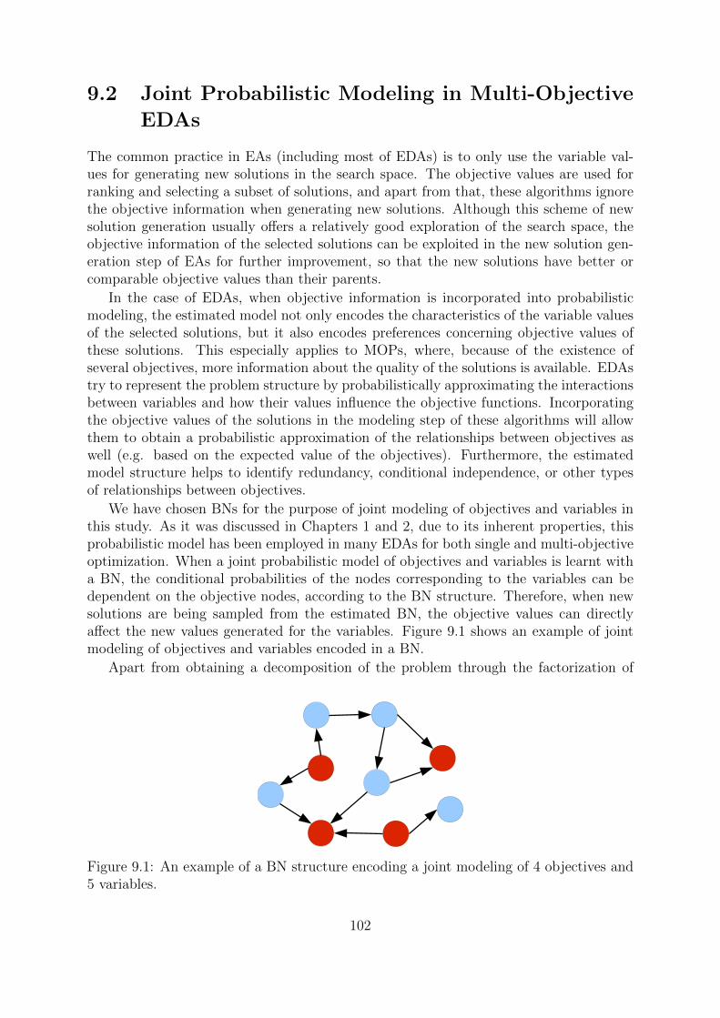
9.2 Joint Probabilistic Modeling in Multi-Objective

EDAs

The common practice in EAs (including most of EDAs) is to only use the variable val-ues for generating new solutions in the search space. The objective values are used forranking and selecting a subset of solutions, and apart from that, these algorithms ignorethe objective information when generating new solutions. Although this scheme of newsolution generation usually offers a relatively good exploration of the search space, theobjective information of the selected solutions can be exploited in the new solution gen-eration step of EAs for further improvement, so that the new solutions have better orcomparable objective values than their parents.

In the case of EDAs, when objective information is incorporated into probabilisticmodeling, the estimated model not only encodes the characteristics of the variable valuesof the selected solutions, but it also encodes preferences concerning objective values ofthese solutions. This especially applies to MOPs, where, because of the existence ofseveral objectives, more information about the quality of the solutions is available. EDAstry to represent the problem structure by probabilistically approximating the interactionsbetween variables and how their values influence the objective functions. Incorporatingthe objective values of the solutions in the modeling step of these algorithms will allowthem to obtain a probabilistic approximation of the relationships between objectives aswell (e.g. based on the expected value of the objectives). Furthermore, the estimatedmodel structure helps to identify redundancy, conditional independence, or other typesof relationships between objectives.

We have chosen BNs for the purpose of joint modeling of objectives and variables inthis study. As it was discussed in Chapters 1 and 2, due to its inherent properties, thisprobabilistic model has been employed in many EDAs for both single and multi-objectiveoptimization. When a joint probabilistic model of objectives and variables is learnt witha BN, the conditional probabilities of the nodes corresponding to the variables can bedependent on the objective nodes, according to the BN structure. Therefore, when newsolutions are being sampled from the estimated BN, the objective values can directlyaffect the new values generated for the variables. Figure 9.1 shows an example of jointmodeling of objectives and variables encoded in a BN.

Apart from obtaining a decomposition of the problem through the factorization of

Figure 9.1: An example of a BN structure encoding a joint modeling of 4 objectives and5 variables.

102

joint probability distribution, joint modeling performs an implicit variable selection foreach of the objectives considering the MB of the objective nodes in BN structure. Incontinuous domains, assuming a Gaussian distribution for the joint vector of variablesand objectives, (X,Q) = (X1, . . . , Xn, Q1, . . . , Qm), where Qj is a random variable takingvalues from the range of the jth objective function, i.e. Qj = fj(X), a GBN is estimatedas the probabilistic model.

9.2.1 Discussion

By estimating a probability distribution from a set of selected solutions, EDAs try tomodel the regions of the search space that are represented by these solutions. In doingso, these algorithms assume that the selected solutions represent promising regions ofthe search space, and that further exploration and exploitation of these regions (whichin EDAs are interchanged automatically based on the distribution of the solutions) willguide the search toward optimal solutions. Using probabilistic models will allow EDAs toboth discover and take advantage of the useful regularities in the set of selected solutionsfor better optimization, as it has been explained in Chapter 2.

In a typical EDA, all of the solutions used for estimating the probabilistic model areequally weighted and are treated in the same way. In other words, the quality of solutionsare not taken into consideration in the probabilistic modeling of the search space. Instead,it is the density of the selected solutions in the search space that drives model estimationand therefore the algorithm will be completely blind to the quality of the new candidatesolutions sampled from the estimated model.

When the quality information of the solutions is integrated into model estimation, itadds another extent to the probabilistic model concerning the regions of the objectivespace that correspond to the objective values of the selected solutions. Since the solutionsare often selected for model learning according to their objective values, the estimatedmodel encodes best found regions of the objective space. Hence, the new candidatesolutions sampled from the joint probabilistic model are more likely to fall in these regionsof the objective space, essentially helping the algorithm to find better candidate solutionsin each generation. Moreover, isolated solutions with good objective values have a betterchance of reproduction when estimating a joint probabilistic model. This is because sucha model can encode the relationships between the promising regions in the objective andsearch spaces, and thus sampling different regions of the search space will be influenced(i.e. controlled) by their approximated qualities.

The employment of similar approaches in a few single-objective EDAs like EBCOAMiquelez et al. [2004, 2006] and DEUM Shakya and McCall [2007] is already shown tohelp achieving better optimization results. However, with the existence of more thanone objective in multi-objective optimization, the joint probabilistic model estimationshould account for several, possibly conflicting objective values of the solutions. Usingan expressive probabilistic model like BN allows to capture the relationships betweendifferent objectives when modeling promising regions of the objective space, and thereforethe EDA based on such a model can adaptively combine the distinct quality informationavailable when sampling new candidate solutions from the estimated probabilistic model.

103

Figure 9.2: An overview of the proposed algorithm

9.3 JGBN-EDA for Continuous Multi-Objective Op-

timization

Figure 9.2 shows the outline of the proposed algorithm based on joint modeling of ob-jectives and variables, called JGBN-EDA. After selecting a subset of solutions in thepopulation, a dataset of joint variable-objective values is formed by appending the objec-tive values of the selected solutions to their variable values. In each generation, a GBNis estimated from this dataset, encoding both objectives and variables, and it is usedto sample new values for the variables when generating new solutions. The generatedsolutions are then evaluated to obtain their true objective values, though approximatedobjective values for the offspring solutions are also given by the estimated joint model.The solution ranking and selection method as well as the estimation of joint probabilisticmodel are explained in more detail in the following sections.

9.3.1 Solution Ranking and Selection

The extensively used non-dominated sorting algorithm [Deb et al., 2002a], based onPareto dominance relation and crowding distances in the objective space, is adoptedin JGBN-EDA for solution ranking. This algorithm first sorts the solutions into differentPareto sets and then within each set the solutions are ordered according to their crowding

104

distances, favoring solutions that are in less populated regions of the objective space topromote diversity of the approximated Pareto front. The crowding distance measureshow close is (using Euclidean distance) each solution to its neighbors with regard to eachof the objectives.

After obtaining a total ordering between all solutions with the non-dominated sortingalgorithm, a subset of solutions is selected using truncation selection. For this purpose,the Pareto fronts are added to the set of selected solutions one-by-one according to theirranks and starting from the Pareto set with the best rank. When we reach a Paretoset which cannot be added completely anymore, due to the size limit determined byparameter τ ∈ (0, 1) of truncation selection, a subset of its solutions are selected accordingto their crowding distances. Here, we use a slightly modified version of the original non-dominated sorting algorithm for selecting this subset from the partially added Pareto set.The solutions are selected one-by-one for addition according to their crowding distancesand after removing each individual, the crowding distance of the solutions remaining inthe Pareto set are recomputed [Zhang et al., 2008].

Another sorting algorithm used in the proposed JGBN-EDA is the weighted sumapproach. Given a weight vector w = (w1, . . . , wm) showing the importance of eachobjective function, each solution xi is assigned a value computed as:

m∑j=1

wj fj(xi), (9.1)

where fj denotes a normalized value of the jth objective function considering the objectivevalues in the population. The solutions are then ordered with respect to these weightedsums and the subset with the smallest values (assuming minimization) is selected. Here,we consider an uninformed version of this approach where all objectives are equallyweighted.

9.3.2 Joint Model Learning and Sampling

We use the algorithm described in Section 6.3 to learn a GBN from the joint dataset ofvariable-objective values. In comparison to the case when only variable values are usedfor model estimation, the dimensionality of this dataset has increased while the numberof samples is the same. As it was discussed in Chapter 4, this can affect the estimationof MGD parameters needed to compute the parameters of the conditional probabilitiesin GBN nodes. Therefore, regularization techniques are especially useful for the jointmodeling scenario.

In the joint modeling used in JGBN-EDA, all of the values in the given joint datasetare standardized to have a zero mean and a variance of one, simplifying the GBN learningprocess and reducing the number of parameters encoded in each node [Schmidt et al.,2007]. The standardized joint dataset is then used for estimating the parameters ofan MGD. Specifically, we use the shrinkage estimation method [Schafer and Strimmer,2005b], with a diagonal target matrix and no shrinkage on the diagonal entries, to obtaina regularized estimation of MGD’s covariance matrix. Based on these estimations, theparameters of conditional probabilities in GBN nodes are computed.

The estimated GBN can be sampled like other BNs with PLS algorithm. However,since the model also consists of objective nodes, we consider two different strategies for

105

sampling. In the first approach, a set of expected or desired objective values are insertedinto the model as evidence, when generating new values for the variables. This kindof information can be provided, for example, by a DM or a domain expert. Anotherpossibility, when such information is not available, is to use the objective values of theselected solutions, favoring new solutions with objective values close to those of theselected solutions.

In the second approach, objective nodes are treated the same as variable nodes andnew values are generated for both variables and objectives when sampling the estimatedmodel. In this way, the PLS algorithm can take into account the approximated values forobjectives, leading to a sampling which is more consistent with the probabilities encodedin the estimated model. Our experimental results have shown better exploration of thesearch space with this method, and therefore we use the second approach in JGBN-EDA.It should be noted that it is also possible to use a hybrid approach based on a combinationof these two methods.

As it is common for the search in continuous spaces with EAs, some of the generatedvalues may not be in the acceptable domain of their corresponding variables. To repair theinvalid variable values (values not in the variable domain) of the new offspring solutions,they are reset to a random value in the acceptable domain of the variable. More precisely,to increase the possibility of appropriate value reseting, the invalid value is replaced witha random value generated between the variable’s conditional mean (estimated with GBN)and the violated (upper or lower) domain-bound.

Since the number of objectives in MOPs are often of the same order as the number ofvariables (i.e. n ' m), according to the time complexity analysis provided in Section 5.3.2,the computational time requirement for estimating a GBN of the joint variable-objectivevector is bounded by O(kN(2n)2+k(2n)4), which adds to the coefficient of the complexityrather than its degree. In fact, in many MOPs the number of objectives is far smallerthan the number of variables, and thus the additional overhead for integrating objectivesdoes not considerably increase the computational time of model estimation or sampling.

9.4 Experiments

In this section the proposed algorithm is tested on a set of well-known benchmark MOPsto study its behavior and compare its performance with other EMO algorithms. Espe-cially, to test the influence of learning a joint model in our proposed algorithm whenincluding objectives, we compare it with a version that does not perform joint modelingand only considers variable values for learning the probabilistic model. In fact, this ver-sion of the algorithm is very similar to other BN-based EDAs found in the literature (e.g.EGNA [Larranaga et al., 2000a]). We refer to this version as GBN-EDA to differentiateit from the algorithm based on joint modeling.

The proposed algorithm is also compared with NSGA-II [Deb et al., 2002a] which isconsidered as a standard reference in many of the studies on EMO algorithms [Zitzleret al., 2003; Coello Coello et al., 2007], and RM-MEDA [Zhang et al., 2008], a multi-objective EDA shown to outperform several EMO algorithms on different benchmarkMOPs. NSGA-II is a multi-objective GA which uses simulated binary crossover [Deb andAgrawal, 1995] and polynomial mutation [Deb and Goyal, 1996] as its genetic operators

106

for search in continuous spaces, and non-dominated sorting algorithm for solution rankingand selection. RM-MEDA assumes a certain type of smoothness for Pareto optimal setand in each generation learns an m−1-dimensional piece-wise continuous manifold whichis then used to generate new samples. The solutions are ranked using the non-dominatedsorting algorithm.

All of the algorithms are implemented in Matlab R©. In each generation, all of thealgorithms select a subset of solution which are used for reproducing new offspring so-lutions, either using genetic operators or with estimating and sampling a probabilisticmodel. However, in contrast to the other algorithms which employ an elitist techniqueto decide which solutions in the population should be replaced by the newly generatedoffspring solutions, RM-MEDA just replaces the whole population with the offspring so-lutions. JGBN-EDA and GBN-EDA were tested with both non-dominated sorting andweighted sum approaches for solution ranking and selection. Since the results obtainedwith the weighted sum approach were superior to those obtained with the non-dominatedsorting, which is also reported by others [Corne and Knowles, 2007; Garza-Fabre et al.,2009], therefore, unless otherwise stated, the results presented here are those obtainedwith weighted sum approach. Nevertheless, in the replacement step, the non-dominatedsorting algorithm is used for elitist selection.

9.4.1 WFG Test Problems

Huband et al. [2006] reviewed many of the benchmark MOPs proposed in the literaturelike ZDT [Zitzler et al., 2000], DTLZ [Deb et al., 2002b] and OKA [Okabe et al., 2004a],and based on the analysis of these problems, they proposed a new set of MOPs called thewalking fish group (WFG) problems. These MOPs have a diverse set of properties foundin real-world problems and, therefore, can be a great challenge for any multi-objectiveoptimization algorithm. Each objective function fj of an MOP in this benchmark isdefined as

minz

fj(z) = D · zm + Sj · hj(z1, . . . , zm−1), (9.2)

where D and Sj are scaling factors and hj(·) is a shape function, meaning that it willdetermine the shape of the Pareto optimal front of an MOP (e.g. concave, convex,etc.) together with the shape functions in the definition of other objective functionsof that MOP. z = (z1, . . . , zm) is an m-dimensional vector of parameters obtained byapplying a number of transformation functions, like shifting, biasing or reduction, to then-dimensional input solution x ∈ D.

The vector of parameters is composed of two parts: the first m − 1 parameters,z1, . . . , zm−1, are obtained from the first k variables of the input solution, called positionvariables (they specify the location of the input solution mapping in the objective space).The last parameter (zm) is obtained from the last l variables of the input solution, calledthe distance variables (they determine the proximity of the input solution mapping in theobjective space to the Pareto optimal front). In all WFG problems we have n = k + l,and to simplify the application of transformation functions on the input solution, k isassumed to be a multiple of m− 1 and l should be an even number.

In all of the 9 MOPs of this benchmark, the number of both objectives and variablescan be scaled, with dissimilar domains for the variables and different Pareto optimal

107

Table 9.1: Experimental settings for the WFG problems

No. Objectives 5 10 20

No. Variables 28 50 50

Population Size 600 1000 1500

Max. No. Evaluations 1.5× 105 3× 105 7.5× 105

No. Runs 25 25 10

trade-off magnitudes for the objectives. Except the first three MOPs, the rest of WFGproblems have a concave Pareto optimal front. WFG1 has a mixed convex-concave front,WFG2 has a disconnected convex front, and WFG3 has a degenerated one-dimensionallinear front. For most of these MOPs, the optimal solution of objectives is shifted awayfrom zero to neutralize any bias of the optimization algorithms towards smaller valuesof the variables. Moreover, in many of the WFG problems, the objective functions areinseparable, requiring the optimization algorithm to consider the relationships betweenvariables. Other properties like multi-modality and deception are also present in theobjective functions of these MOPs.

9.4.2 Experimental Design

The quality of the Pareto fronts approximated by each algorithm is evaluated with theinverted generational distance (IGD) [Coello Coello and Cortes, 2005] indicator. This in-dicator accounts for both the diversity of the approximated front as well as its convergenceto the Pareto optimal front. Given a set of points F ∗, representing a well-distributed sam-pling of the Pareto optimal front of an MOP, the IGD value for an approximated Paretofront F is computed as:

IGDF ∗(F ) =

∑s∈F ∗

min∀s′∈F

d(s, s′)

|F ∗|(9.3)

where d(·, ·) gives the Euclidean distance between two points. A smaller value for thisindicator means a better approximation. The statistical significance in the differencesbetween the results is checked with the Kruskal-Wallis test [Kruskal and Wallis, 1952].Kruskal-Wallis test performs a non-parametric one-way analysis of variance (ANOVA)to accept or reject the null hypothesis that independent samples of two or more groupscome from distributions with equal medians, and returns the p-value for that test. Thetest significance level is set to 0.05 in our comparisons.

We have tested three different numbers of objectives with respectively different numberof variables for the WFG problems to keep the computational costs of the experimentsin an affordable level. The details of the experimental setup, which are equally setfor all of the tested EMO algorithms, are given in Table 9.1. To have an idea of thePareto fronts approximated by these algorithms, in Figure 9.3 we have shown the finalPareto fronts obtained by the algorithms for some of the tested MOPs (WFG2, WFG4,WFG6 and WFG7) with 3 objectives, 20 variables and a population size of 200. Therepresented fronts for each algorithm are selected between 25 independent runs using the

108

01

23 0

12

34

0

1

2

3

4

5

6

7

WFG2

NSGA−II

RM−MEDA

GBN−EDA

JGBN−EDA

00.511.522.5

0

50

1

2

3

4

5

6

7

WFG4

NSGA−II

RM−MEDA

GBN−EDA

JGBN−EDA

00.511.522.5

−5

0

5

−1

0

1

2

3

4

5

6

7

WFG6

NSGA−II

RM−MEDA

GBN−EDA

JGBN−EDA

00.511.522.5

−50

5−1

0

1

2

3

4

5

6

7

WFG7

NSGA−II

RM−MEDA

GBN−EDA

JGBN−EDA

Figure 9.3: Typical Pareto fronts obtained by different algorithms for WFG problemswith 3 objectives.

coverage indicator. This indicator computes the percentage of solutions in a Pareto setB dominated by the solutions in another Pareto set A

A coverage of B =

∣∣{x ∈ B | ∃y ∈ A,y ≺ x}∣∣|B|

.

9.4.3 Results

Figure 9.4 shows the results obtained by each of the algorithms for WFG problems with 5objectives. As it can be seen in the figure, the incorporation of objectives in the modelingof JGBN-EDA enables this algorithm to obtain a (significantly) better performance onmost of the problems, according to the IGD indicator. A direct comparison of GBN-EDAand JGBN-EDA shows the effectiveness of joint modeling where except for WFG5 andWFG9 problems, the latter algorithm can obtain significantly better results on the testedMOPs (p = 0.05).

WFG5 is composed of separable and deceptive functions while WFG9 consists of anon-separable, biased, multi-modal and deceptive functions. According to the presented

109

2

2.5

3

3.5

4

4.5

NSGA−II RM−MEDA GBN−EDA JGBN−EDA

WFG1

IGD

0.4

0.6

0.8

1

1.2

NSGA−II RM−MEDA GBN−EDA JGBN−EDA

WFG2

IGD

1

1.05

1.1

1.15

NSGA−II RM−MEDA GBN−EDA JGBN−EDA

WFG3

IGD

0.7

0.75

0.8

0.85

0.9

0.95

1

1.05

NSGA−II RM−MEDA GBN−EDA JGBN−EDA

WFG4

IGD

1.1

1.15

1.2

1.25

1.3

1.35

1.4

1.45

NSGA−II RM−MEDA GBN−EDA JGBN−EDA

WFG5

IGD

0.7

0.8

0.9

1

1.1

1.2

1.3

NSGA−II RM−MEDA GBN−EDA JGBN−EDA

WFG6

IGD

0.6

0.7

0.8

0.9

1

1.1

1.2

1.3

NSGA−II RM−MEDA GBN−EDA JGBN−EDA

WFG7

IGD

0.7

0.8

0.9

1

1.1

1.2

1.3

1.4

NSGA−II RM−MEDA GBN−EDA JGBN−EDA

WFG8

IGD

0.7

0.75

0.8

0.85

0.9

0.95

1

1.05

NSGA−II RM−MEDA GBN−EDA JGBN−EDA

WFG9

IGD

Figure 9.4: Comparison of the performance of different algorithms on WFG problemswith 5 objectives.

results, for deceptive functions the information provided by objectives does not have agreat impact on the joint probabilistic model estimated in JGBN-EDA for generatingbetter solutions. Also, the algorithm is not able to properly utilize the separability ofvariables in WFG5 to obtain better fronts. However, the results obtained for WFG9 showsthat non-separability and multi-modality in the functions of this problem are completelyaddressed with the probabilistic modeling used in JGBN-EDA and GBN-EDA, makingthem better performers in comparison to the other two competitor algorithms for thisproblem.

As the number of objectives grows to 10 and 20 (Figures 9.5 and 9.6), the performanceof the proposed algorithm, measured by IGD indicator, deteriorates in comparison toother algorithms. The other two competitor algorithms also show a diverse behavioron different number of objectives. While the fronts approximated by NSGA-II on 10-objective MOPs are not comparable to those of other algorithms, this algorithm is ableto find significantly better results for most of the problems with 20 objectives. RM-MEDAis showing an apposite behavior, obtaining better results on the 10-objective case. For

110

3

4

5

6

7

NSGA−II RM−MEDA GBN−EDA JGBN−EDA

WFG1

IGD

1.5

2

2.5

3

NSGA−II RM−MEDA GBN−EDA JGBN−EDA

WFG2

IGD

2.5

3

3.5

NSGA−II RM−MEDA GBN−EDA JGBN−EDA

WFG3

IGD

1.6

1.8

2

2.2

2.4

2.6

2.8

3

NSGA−II RM−MEDA GBN−EDA JGBN−EDA

WFG4

IGD

2.6

2.8

3

3.2

3.4

3.6

NSGA−II RM−MEDA GBN−EDA JGBN−EDA

WFG5

IGD

2.2

2.4

2.6

2.8

3

3.2

NSGA−II RM−MEDA GBN−EDA JGBN−EDA

WFG6

IGD

2

2.5

3

NSGA−II RM−MEDA GBN−EDA JGBN−EDA

WFG7

IGD

1.8

2

2.2

2.4

2.6

2.8

3

3.2

NSGA−II RM−MEDA GBN−EDA JGBN−EDA

WFG8

IGD

1.8

2

2.2

2.4

2.6

2.8

NSGA−II RM−MEDA GBN−EDA JGBN−EDA

WFG9

IGD

Figure 9.5: Comparison of the performance of different algorithms on WFG problemswith 10 objectives.

these high number of objectives the performance of the proposed JGBN-EDA seems tobe less varying when compared with other algorithm on both 10- and 20-objective WFGproblems.

The recombination operators employed in NSGA-II allow obtaining better approxi-mations for the mixed concave-convex front of WFG1 with some flat regions in the Paretoset. The inclusion of objective values in the modeling of JGBN-EDA has a major influ-ence in improving the performance on this MOP when compared to GBN-EDA. On theother hand, the disconnected front of WFG2 causes a diverse performance of NSGA-II,while the EDAs are almost performing similar when the number of objectives is 10 and20. The significantly better performance of JGBN-EDA on WFG9 is also repeated for 10and 20 objectives.

It seems that when the number of objectives increase to a high number (e.g. 20),the probabilistic modeling in EDAs is overfitted for small populations and can not helpthese algorithms to make progress in the search space. In fact for such a large number ofobjectives small population sizes may not be sufficient to represent a good approximation

111

5

10

15

20

25

30

NSGA−II RM−MEDA GBN−EDA JGBN−EDA

WFG1

IGD

−0.5

0

0.5

1

1.5

2

2.5

3

NSGA−II RM−MEDA GBN−EDA JGBN−EDA

WFG2

IGD

3

4

5

6

7

8

NSGA−II RM−MEDA GBN−EDA JGBN−EDA

WFG3

IGD

1

1.5

2

2.5

NSGA−II RM−MEDA GBN−EDA JGBN−EDA

WFG4

IGD

2

2.5

3

3.5

4

NSGA−II RM−MEDA GBN−EDA JGBN−EDA

WFG5

IGD

1

1.2

1.4

1.6

1.8

2

2.2

NSGA−II RM−MEDA GBN−EDA JGBN−EDA

WFG6

IGD

0.6

0.8

1

1.2

1.4

1.6

1.8

NSGA−II RM−MEDA GBN−EDA JGBN−EDA

WFG7

IGD

1

1.2

1.4

1.6

1.8

2

NSGA−II RM−MEDA GBN−EDA JGBN−EDA

WFG8

IGD

1.5

2

2.5

3

3.5

NSGA−II RM−MEDA GBN−EDA JGBN−EDA

WFG9

IGD

Figure 9.6: Comparison of the performance of different algorithms on WFG problemswith 20 objectives.

of the Pareto front. This issue should also be considered for representing the Paretooptimal front with a sample set which is used for computing the IGD quality indicator.Although in this study we have used sample sets with several hundred thousands ofpoints for this purpose, some regions of the Pareto optimal front may still not be coveredproperly.

9.5 Conclusions

A joint modeling of objectives and variables was proposed to be used for multi-objectiveoptimization in this chapter. The proposed EDA, called JGBN-EDA, learns a GBN toencode the relationships between variables and objectives, from a joint variable-objectivedataset formed by appending the objective values to the variables values of the solutions.The estimated probabilistic model encodes both variable and objective nodes and thus inthe sampling process new values for variables can be generated using the objective valueswhen such dependencies are encountered in the model.

112

The performance of the algorithm was tested on a number of test MOPs havingdifferent properties found in real-world problems. The results of comparing two versionsof the algorithm, one utilizing the objectives information and the other not, showedthat the incorporation of objectives in the modeling can help the algorithm to obtainbetter Pareto fronts on some of the problems. The algorithm was also compared withtwo other algorithms, NSGA-II as a standard EMO algorithm and RM-MEDA whichis a competitive multi-objective EDA, and the obtained results indicated the promisingperformance of the proposed approach to probabilistic modeling in EDAs.

The algorithm was not able to detect the correct search bias for some MOPs withdeceptive objective functions using the proposed joint modeling. Moreover, for someof the problems the algorithm was not able to obtain competitive fronts when thereare a high number of objectives in the MOP. The effect of proper population sizing onthe performance of the algorithm specially for many objectives problems should also bestudied in more detail. The information provided by dependencies between the objectivescan be further investigated to help revealing their relationships in problems with manyobjectives. Nevertheless, the proposed algorithm can be seen as an alternative for usingprobabilistic modeling in multi-objective optimization.

113

114

Chapter 10

Multi-Dimensional BayesianNetwork Modeling for EvolutionaryMulti-Objective Optimization

10.1 Introduction

In the previous chapter, we studied joint probabilistic modeling of variables and objectivesfor multi-objective optimization. This type of modeling offered a new way for analyzingthe relationships between variables and objectives, and was shown to be advantageousfor solution search compared with learning a model of only variables. In this chapter, weextend this study using a specific probabilistic modeling employed in the area of multi-dimensional classification. In this type of problems, each instance or data point is assigneda vector of class-values, and the goal of model learning is to predict the class-value vectorsof new instances. On the other hand, in multi-objective EDAs, each solution is assigneda vector of objective values, and the goal of model learning is to generate new solutionswith better objective values from the probabilistic model. Clearly, there are similaritiesbetween the two problems which motivates the use of similar probabilistic modeling inboth.

We adapt multi-dimensional BN classifiers [de Waal and van der Gaag, 2007; Bielzaet al., 2011b] for joint modeling of variables and objectives. Using this type of proba-bilistic model in joint modeling, three distinct types of relationships can be captured:(i) the interactions between variables, as in other EDAs, (ii) the relationships betweenvariables and objectives, and (iii) the relationships between objectives. The clear dis-tinction between these three types of relationships, of which the last two are capturedbecause of joint modeling, allows a better analysis and interpretation of the estimatedmodel structures, and since it is closer to the semantics of MOPs, it provides the DMwith an approximation of the MOP structure, i.e. the relationships among variables andobjectives of the MOP. Moreover, as it will be shown later, with this type of probabilis-tic model, EDA is able to find better Pareto fronts for many of the tested MOPs. Theproposed method and related discussions are also appeared in [Karshenas et al., 2012b].

As reviewed in Chapter 2, BN classifiers have been previously used as probabilisticmodels in EDAs for single-objective optimization in EBCOA [Miquelez et al., 2004, 2006].However, there are several key differences between EBCOA and the algorithm presented

115

Figure 10.1: An example of a multi-dimensional Bayesian network structure.

here. First, the presence of multiple objectives in an MOP increases the informationabout the quality of solutions (possibly contradictory) that should be addressed duringmodeling. Second, in continuous domains, instead of classifying the solutions into disjointclasses which may blur the differences in the quality of the solutions, we directly use thecontinuous objective values in joint model learning. Third, in contrast to a fixed depen-dency between the objectives and variables, the algorithm presented here dynamicallylearns the relationships between the objectives and variables. In this way, the model canselect a subset of variables that has more influence on each objective.

10.2 Multi-Dimensional Bayesian Network Classifiers

When the classification problem involves more than one class variable, each instance ofthe dataset is assigned a vector of class-values c = (c1, . . . , cm). Then, to determinethe class-value vector of an unlabeled instance given its feature values x = (x1, . . . , xn),a multi-dimensional BN (MBN) can be estimated from a training dataset and used tocompute the class-value vector with the highest posterior probability for this instance:

c∗ = arg maxc

P (c | x). (10.1)

Figure 10.1 shows an example of an MBN structure. In this type of model, the nodesare organized in two separate layers: the top layer comprises class variables and thebottom layer contains feature variables. The set of arcs in the structure is partitionedinto three subsets, resulting in the following subgraphs:

• the class subgraph, containing the class nodes and the interactions between them,

• the feature subgraph, comprising the feature variables and their relations, and

• the bridge subgraph, depicting the top-down relationships between class and featurenodes.

Depending on the order of relationships and the structure learnt in the class and bridgesubgraphs, different types of MBN classifiers can be considered: without any edges likeNB, directed trees like TAN, polytrees or even completely unrestricted.

This probabilistic model can answer several types of queries: the vector of class-valuesof a given data point, the most probable feature values for a given vector of class-values,

116

and the most probable values for a subset of features or classes given the value of theothers. Considering the similarity between multi-dimensional classification and multi-objective optimization, the respective questions will be: what are the estimated objectivevalues of a given solution, what is the most probable values for the variables of thesolution which results in a specific value-setting for the objectives, and, having found theproper values of some objectives or variables, what will be the most probable values ofthe others.

10.3 MBN-EDA: An EDA Based on MBN Estima-

tion

In this section we propose a multi-objective EDA which uses MBNs for joint modeling ofvariables and objectives, called MBN-EDA. The variables are modeled as feature nodesand objectives as continuous-valued class nodes (regression response nodes). The featuresubgraph of MBN encodes the relationships between variables like the models learnt byother BN-based EDAs [Schwarz and Ocenasek, 2001; Khan et al., 2002; Laumanns andOcenasek, 2002; Katsumata and Terano, 2003; Pelikan et al., 2005; Ahn and Ramakrishna,2007]. However, the bridge and class subgraphs, encode new types of relationships asthe result of joint modeling of variables and objectives. The bridge subgraph showsthe interactions between each objective and the variables (selects a subset of relevantvariables for each objective), and the class subgraph represents the relationships directlybetween objectives. The joint probability distribution encoded in the probabilistic modelof MBN-EDA can be represented as

ρ (x1, . . . , xn, q1, . . . , qm) =n∏i=1

ρ(xi|pai) ·m∏j=1

ρ(qj|pa′j), (10.2)

where Pai ⊆{{X \Xi} ∪Q

}and Pa′j ⊆ {Q \Qj} are the parents of each variable and

objective, respectively, according to the MBN structure, and pai and pa′j represent oneof their possible value-settings. q = (q1, . . . , qm) denotes a possible value-setting for theobjective variables Q = (Q1, . . . , Qm) corresponding to solution x = (x1, . . . , xn).

The general framework of MBN-EDA is the same as the one shown for joint modellearning in Figure 9.2 of the previous section. However, the solution ranking methodsand the probabilistic model used in this algorithm are different and are discussed in thefollowing sections.

10.3.1 Solution Ranking and Selection

In contrast to single objective optimization, where the objective values can be used di-rectly to rank solutions, the existence of multiple objectives in MOPs necessitates theapplication of an intermediate function of the form g : F ⊆ Rm 7→ F′ ⊆ R, so that itsoutput can be used to rank the solutions. In the previous chapter, the commonly usednon-dominated sorting algorithm was employed to sort the solutions for selection. How-ever, it has been shown that the effectiveness of this ranking method decreases as thedimensions of the objective space increase [Hughes, 2005; Ishibuchi et al., 2008; Aguirre

117

and Tanaka, 2010]. Finding efficient ranking methods for many-objective optimizationis the topic of ongoing research, and several methods have been proposed so far in theliterature. In this study, we adopt some of the methods proposed for this purpose, whichwere shown to result in good performance for evolutionary many-objective optimization[Corne and Knowles, 2007; Garza-Fabre et al., 2009, 2010a,b].

Let x and y, where x,y ∈ D, be two solutions of a population of solutions D to agiven MOP. Then, beside the weighted sum approach defined in Section 9.3.1, denotedas gWS, the following three ranking methods are employed in MBN-EDA:

• Distance to the best objective values f ∗ = (f ∗1 , . . . , f∗m) for each solution, using

some distance measure d(·, ·) in the objective space (e.g. Euclidean distance):

gDB(x) = d(f ∗, f(x)

). (10.3)

When the best objective values are not known beforehand (which is usually thecase), the best objective values achieved so far (considering each objective sepa-rately) in the current population can be used, i.e. the best value f ∗j for the jthobjective function is

f ∗j = minx∈D

fj(x).

• Global detriment or the total gain lost by each solution against other solutions ofthe population:

gGD(x) =∑

∀y∈D,y 6=x

gain(y,x), (10.4)

where the function gain(·, ·) computes the gain of a solution over another in theobjective space (assuming minimization):

gain(x,y) =m∑j=1

max{0, fj(y)− fj(x)}. (10.5)

• Profit of the gain obtained from each solution against other solutions of the popu-lation:

gPG(x) = maxy∈D,y 6=x

gain(x,y)− maxy∈D,y 6=x

gain(y,x). (10.6)

When any of the above gXX functions is applied to the solutions in a population D, asingle value is assigned to each of the solutions served for their sorting. Given a sortedlist of solutions, any selection mechanism can be used for selecting a subset. Similar tothe previous chapter, a truncation selection mechanism is used in MBN-EDA.

10.3.2 MBN Learning and Sampling

Here, we explain probabilistic modeling in MBN-EDA for continuous multi-objectiveoptimization, assuming a Gaussian distribution for the joint vector of variables and ob-jectives. In continuous domains, MBN is implemented with a GBN. Instead of learningthe structure of each of the MBN subgraphs separately, we use a learning procedure verysimilar to the one explained in Section 9.3.2 of the previous chapter. Since the structure

118

of the bridge subgraph is constrained to only include top-down interactions between vari-able and objective nodes, the greedy search is performed in a restricted DAG space, andthe corresponding sub-matrix of the covariance matrix is explicitly set to zero. The BICscore of an MBN structure based on log-likelihood and computed from a joint dataset of

variable-objective values{(x1,f(x1)

), . . . ,

(xN ,f(xN)

)}is

N∑k=1

( n∑i=1

log(p(xk<Xi> | xk<Pai>)

)+

m∑j=1

log(p(fj(xk) | xk<Pa′j>)

))− 1

2log (N)

( n∑i=1

|Pai|+m∑j=1

|Pa′j|+ 2(n+m)), (10.7)

where xk<Pai> and xk<Pa′j> are the value-settings for the parents of respectively theith variable and jth objective nodes, according to the MBN structure, in the kth jointvariable-objective individual of the dataset. |Pai| ≤ n + m − 1 and |Pa′j| ≤ m − 1show the number of parents for the ith variable and jth objective, according to the MBNstructure.

As before, the PLS algorithm is used to sample the estimated MBN for generatingnew solutions. Due to the restrictions imposed on the bridge subgraph in the learningprocess, all objective nodes appear before variable nodes in the topological ordering ob-tained for an MBN. This decreases the number of inconsistent values generated for thevariables when a set of objective values are inserted as evidence during model sampling[Koller and Friedman, 2009]. The second approach to joint model sampling, explainedin Section 9.3.2, is employed in MBN-EDA to take into account the approximated char-acteristics of the objective values (collected from the selected solutions) encoded in themodel.

10.4 Experiments on WFG Test Problems

Following the experimental setup of the previous chapter, in this section we examine theperformance of MBN-EDA and its joint modeling for continuous multi-objective opti-mization of WFG problems. Figure 10.2 shows the final Pareto fronts approximated byNSGA-II, RM-MEDA and MBN-EDA for some of the WFG problems (WFG2, WFG3,WFG4, WFG6, WFG7) with 3 objectives, 20 variables and a population size of 200. Thesefronts are selected, according to the coverage indicator, between 25 independent runs ofeach algorithm when using non-dominated sorting for solution ranking and selection.

To compare the joint probabilistic modeling of variables and objectives performedin MBN-EDA with the one done in JGBN-EDA of the previous chapter, we have com-pared their optimization performance on WFG problems with an increasing number ofobjectives. On some of these problems, the quality of the final Pareto fronts obtainedby the two algorithms, evaluated with IGD indicator, are very similar. However, forsome of the WFG problems, there are considerable differences in the results obtained bythese algorithms. For example, Figures 10.3 and 10.4 show the IGD indicator values ofthe final Pareto fronts obtained by these two algorithms, when using the non-dominatedsorting method for solution ranking and selection, in 25 independent runs for respectively

119

0

1

2

3 0 1 2 3 4 5

0

1

2

3

4

5

6

7

WFG2

NSGA−II

RM−MEDA

MBN−EDA

0

2

40 0.5 1 1.5 2 2.5 3 3.5

−1

0

1

2

3

4

5

6

7

WFG3

NSGA−II

RM−MEDA

MBN−EDA

00.511.522.5

0

5

0

1

2

3

4

5

6

7

WFG4

NSGA−II

RM−MEDA

MBN−EDA

00.511.522.5

0

2

40

1

2

3

4

5

6

7

WFG6

NSGA−II

RM−MEDA

MBN−EDA

00.511.522.5

−5

0

50

1

2

3

4

5

6

7

WFG7

NSGA−II

RM−MEDA

MBN−EDA

Figure 10.2: The Pareto fronts obtained by different algorithm for WFG problems with3 objectives.

120

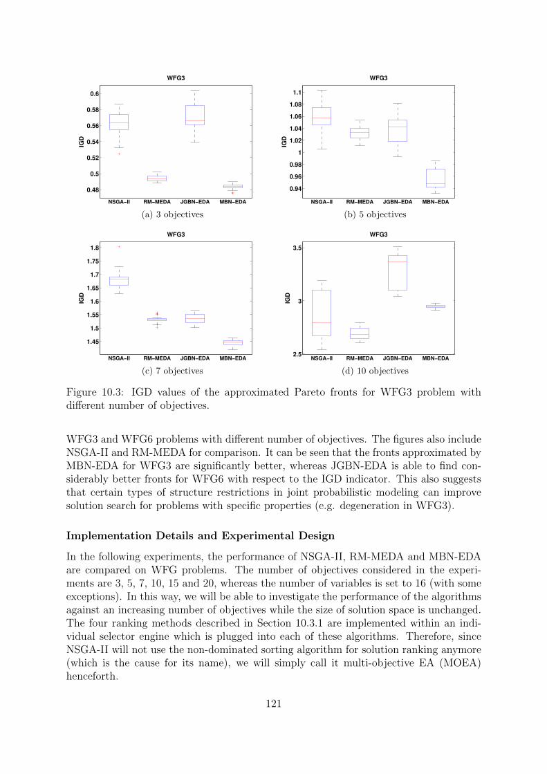
0.48

0.5

0.52

0.54

0.56

0.58

0.6

NSGA−II RM−MEDA JGBN−EDA MBN−EDA

WFG3IG

D

(a) 3 objectives

0.94

0.96

0.98

1

1.02

1.04

1.06

1.08

1.1

NSGA−II RM−MEDA JGBN−EDA MBN−EDA

WFG3

IGD

(b) 5 objectives

1.45

1.5

1.55

1.6

1.65

1.7

1.75

1.8

NSGA−II RM−MEDA JGBN−EDA MBN−EDA

WFG3

IGD

(c) 7 objectives

2.5

3

3.5

NSGA−II RM−MEDA JGBN−EDA MBN−EDA

WFG3

IGD

(d) 10 objectives

Figure 10.3: IGD values of the approximated Pareto fronts for WFG3 problem withdifferent number of objectives.

WFG3 and WFG6 problems with different number of objectives. The figures also includeNSGA-II and RM-MEDA for comparison. It can be seen that the fronts approximated byMBN-EDA for WFG3 are significantly better, whereas JGBN-EDA is able to find con-siderably better fronts for WFG6 with respect to the IGD indicator. This also suggeststhat certain types of structure restrictions in joint probabilistic modeling can improvesolution search for problems with specific properties (e.g. degeneration in WFG3).

Implementation Details and Experimental Design

In the following experiments, the performance of NSGA-II, RM-MEDA and MBN-EDAare compared on WFG problems. The number of objectives considered in the experi-ments are 3, 5, 7, 10, 15 and 20, whereas the number of variables is set to 16 (with someexceptions). In this way, we will be able to investigate the performance of the algorithmsagainst an increasing number of objectives while the size of solution space is unchanged.The four ranking methods described in Section 10.3.1 are implemented within an indi-vidual selector engine which is plugged into each of these algorithms. Therefore, sinceNSGA-II will not use the non-dominated sorting algorithm for solution ranking anymore(which is the cause for its name), we will simply call it multi-objective EA (MOEA)henceforth.

121

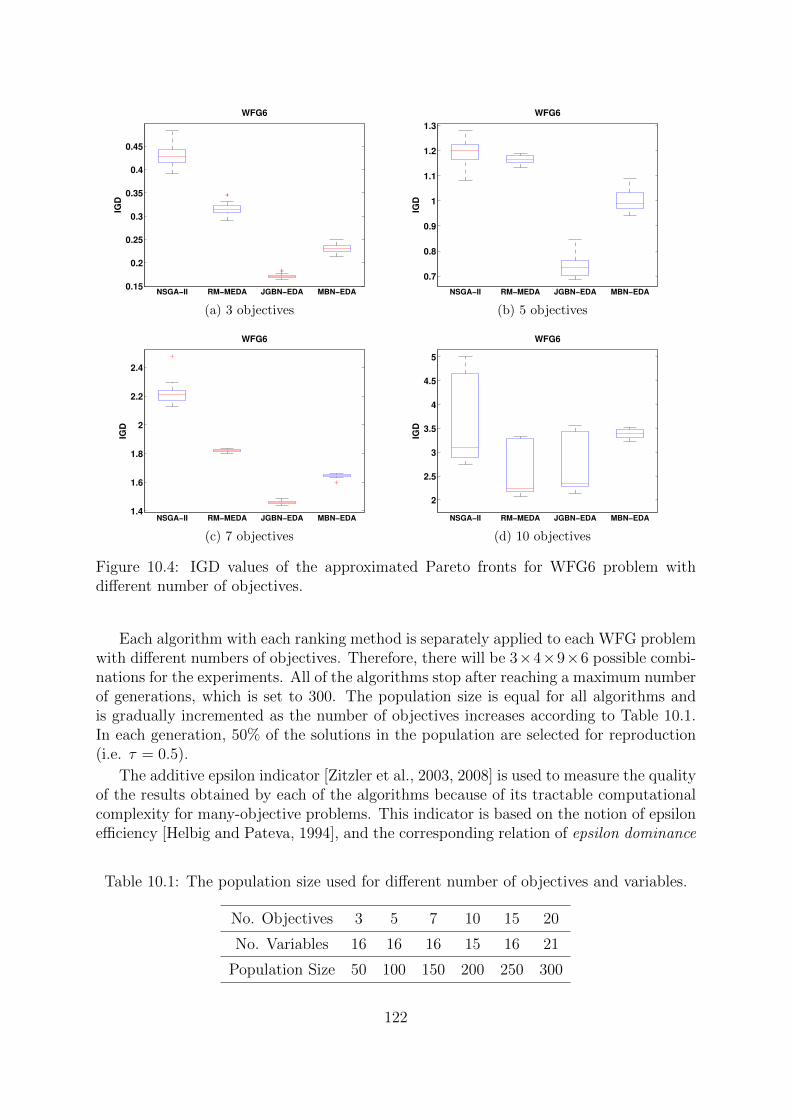
0.15

0.2

0.25

0.3

0.35

0.4

0.45

NSGA−II RM−MEDA JGBN−EDA MBN−EDA

WFG6IG

D

(a) 3 objectives

0.7

0.8

0.9

1

1.1

1.2

1.3

NSGA−II RM−MEDA JGBN−EDA MBN−EDA

WFG6

IGD

(b) 5 objectives

1.4

1.6

1.8

2

2.2

2.4

NSGA−II RM−MEDA JGBN−EDA MBN−EDA

WFG6

IGD

(c) 7 objectives

2

2.5

3

3.5

4

4.5

5

NSGA−II RM−MEDA JGBN−EDA MBN−EDA

WFG6

IGD

(d) 10 objectives

Figure 10.4: IGD values of the approximated Pareto fronts for WFG6 problem withdifferent number of objectives.

Each algorithm with each ranking method is separately applied to each WFG problemwith different numbers of objectives. Therefore, there will be 3×4×9×6 possible combi-nations for the experiments. All of the algorithms stop after reaching a maximum numberof generations, which is set to 300. The population size is equal for all algorithms andis gradually incremented as the number of objectives increases according to Table 10.1.In each generation, 50% of the solutions in the population are selected for reproduction(i.e. τ = 0.5).

The additive epsilon indicator [Zitzler et al., 2003, 2008] is used to measure the qualityof the results obtained by each of the algorithms because of its tractable computationalcomplexity for many-objective problems. This indicator is based on the notion of epsilonefficiency [Helbig and Pateva, 1994], and the corresponding relation of epsilon dominance

Table 10.1: The population size used for different number of objectives and variables.

No. Objectives 3 5 7 10 15 20

No. Variables 16 16 16 15 16 21

Population Size 50 100 150 200 250 300

122

that is defined as

∀x,y ∈ D, x �ε+ y ⇐⇒ ∀fi ∈ F fi(x) ≤ ε+ fi(y). (10.8)

The additive epsilon indicator between two Pareto set approximations A and B is definedas the smallest epsilon value that allows all the solutions in B to be ‘ε+’-dominated byat least one solution in A:

Iε+(A,B) = maxε∈R+{A �ε+ B}, (10.9)

whereA �ε+ B ⇐⇒ ∀y ∈ B, ∃x ∈ A | x �ε+ y.

According to this definition, the additive epsilon indicator for a Pareto set approxi-mation A is obtained using a reference set R

Iε+(A) = Iε+(A,R). (10.10)

This definition implies that smaller values of the epsilon indicator are better. A goodchoice for the reference set R is an approximation of the Pareto optimal set. However, thesize of a good approximation of the Pareto optimal set should increase exponentially withthe number of objectives in the MOP to offer a good coverage of the Pareto optimal front.Therefore, this choice of reference set is impractical for many-objective problems. Thereference set considered here is composed of the endpoint solutions, obtained by settingone of the objectives to its minimum value and the others to their maximum values, plusthe solution representing an approximate compromise between the values of all objectives(e.g., the mean value in the objectives range). The size of this reference set grows onlylinearly with the number of objectives, and the inclusion of endpoints favors those Paretoset approximations that result in a more scattered Pareto front.

Results

Figures 10.5–10.7 show the epsilon indicator value obtained for the Pareto sets approx-imated by each of the algorithms when using different ranking methods, averaged over20 independent runs. The statistical analysis of the results on each of the MOPs withdifferent numbers of objectives is shown in Table 10.2. The non-parametric Friedmantest is used to check for the statistical differences of the algorithms performance [Derracet al., 2011]. When the null hypothesis that all the algorithms have an equal average rankis rejected for a specific problem configuration with a p-value less than 0.05, the entryrelated to the algorithm with the best Friedman rank is shown in bold. The numbers inparentheses show the results of pairwise comparisons using Bergmann-Hommel’s post-hoctest with a significance level of α = 0.05. The first number shows how many algorithmsare significantly worse than the algorithm listed in this column, and the second numbershows how many algorithms are significantly better.

The objectives in WFG1 are unimodal and biased for specific regions of their input.For this problem, MBN-EDA is able to obtain significantly better Pareto set approxima-tions than the other two algorithms. The performance of the algorithm is very similarwhen using the different ranking methods tested in these experiments (Figure 10.5, left

123

3 5 7 10 15 200.5

1

1.5

2

2.5

3WFG1 − Weighted Sum ordering

Ep

sil

on

In

dic

ato

r

# of objectives

MBN−EDA

MOEA

RM−MEDA

3 5 7 10 15 2010

−25

10−20

10−15

10−10

10−5

100

105

WFG2 − Weighted Sum ordering

Ep

silo

n In

dic

ato

r

# of objectives3 5 7 10 15 20

10−20

10−15

10−10

10−5

100

105

WFG3 − Weighted Sum ordering

Ep

silo

n In

dic

ato

r

# of objectives

3 5 7 10 15 200.95

1

1.05

1.1

1.15

1.2

1.25WFG1 − Profit of Gain ordering

Ep

sil

on

In

dic

ato

r

# of objectives3 5 7 10 15 20

0.1

0.2

0.3

0.4

0.5

0.6

0.7

0.8

WFG2 − Profit of Gain ordering

Ep

silo

n In

dic

ato

r

# of objectives3 5 7 10 15 20

10−0.6

10−0.5

10−0.4

10−0.3

10−0.2

WFG3 − Profit of Gain ordering

Ep

sil

on

In

dic

ato

r# of objectives

3 5 7 10 15 200.8

1

1.2

1.4

1.6

1.8

2

2.2WFG1 − Global Detriment ordering

Ep

sil

on

In

dic

ato

r

# of objectives3 5 7 10 15 20

10−6

10−5

10−4

10−3

10−2

10−1

100

WFG2 − Global Detriment ordering

Ep

silo

n In

dic

ato

r

# of objectives3 5 7 10 15 20

10−6

10−5

10−4

10−3

10−2

10−1

100

WFG3 − Global Detriment ordering

Ep

silo

n In

dic

ato

r

# of objectives

3 5 7 10 15 200.5

1

1.5

2

2.5

3WFG1 − Distance to Best ordering

Ep

sil

on

In

dic

ato

r

# of objectives3 5 7 10 15 20

10−20

10−15

10−10

10−5

100

105

WFG2 − Distance to Best ordering

Ep

sil

on

In

dic

ato

r

# of objectives3 5 7 10 15 20

10−15

10−10

10−5

100

105

WFG3 − Distance to Best ordering

Ep

sil

on

In

dic

ato

r

# of objectives

Figure 10.5: The average epsilon indicator values for WFG1 (left column), WFG2 (middlecolumn) and WFG3 (right column) problems.

124

3 5 7 10 15 2010

−3

10−2

10−1

100

101

WFG4 − Weighted Sum ordering

Ep

sil

on

In

dic

ato

r

# of objectives

MBN−EDA

MOEA

RM−MEDA

3 5 7 10 15 2010

−2

10−1

100

101

WFG5 − Weighted Sum ordering

Ep

sil

on

In

dic

ato

r# of objectives

3 5 7 10 15 2010

0

101

102

WFG6 − Weighted Sum ordering

Ep

silo

n In

dic

ato

r

# of objectives

3 5 7 10 15 200.1

0.15

0.2

0.25

0.3

0.35

0.4

0.45

0.5WFG4 − Profit of Gain ordering

Ep

sil

on

In

dic

ato

r

# of objectives

3 5 7 10 15 20

0.7

0.8

0.9

1

1.1

1.2

1.3

1.4WFG5 − Profit of Gain ordering

Ep

sil

on

In

dic

ato

r

# of objectives3 5 7 10 15 20

10−0.5

10−0.4

10−0.3

10−0.2

10−0.1

WFG6 − Profit of Gain ordering

Ep

sil

on

In

dic

ato

r# of objectives

3 5 7 10 15 2010

−3

10−2

10−1

100

101

WFG4 − Global Detriment ordering

Ep

sil

on

In

dic

ato

r

# of objectives

3 5 7 10 15 200

0.2

0.4

0.6

0.8

1

1.2

1.4WFG5 − Global Detriment ordering

Ep

sil

on

In

dic

ato

r

# of objectives3 5 7 10 15 20

10−5

10−4

10−3

10−2

10−1

100

101

WFG6 − Global Detriment ordering

Ep

sil

on

In

dic

ato

r

# of objectives

3 5 7 10 15 2010

−3

10−2

10−1

100

101

WFG4 − Distance to Best ordering

Ep

sil

on

In

dic

ato

r

# of objectives3 5 7 10 15 20

10−2

10−1

100

101

WFG5 − Distance to Best ordering

Ep

sil

on

In

dic

ato

r

# of objectives3 5 7 10 15 20

10−3

10−2

10−1

100

101

102

WFG6 − Distance to Best ordering

Ep

sil

on

In

dic

ato

r

# of objectives

Figure 10.6: The average epsilon indicator values for WFG4 (left column), WFG5 (middlecolumn) and WFG6 (right column) problems.

125

3 5 7 10 15 2010

0

101

102

WFG7 − Weighted Sum ordering

Ep

sil

on

In

dic

ato

r

# of objectives

MBN−EDA

MOEA

RM−MEDA

3 5 7 10 15 200

2

4

6

8

10

12

14WFG8 − Weighted Sum ordering

Ep

sil

on

In

dic

ato

r

# of objectives3 5 7 10 15 20

10−4

10−3

10−2

10−1

100

101

WFG9 − Weighted Sum ordering

Ep

silo

n In

dic

ato

r

# of objectives

3 5 7 10 15 20

10−0.5

10−0.3

10−0.1

100.1

WFG7 − Profit of Gain ordering

Ep

sil

on

In

dic

ato

r

# of objectives3 5 7 10 15 20

10−0.4

10−0.3

10−0.2

10−0.1

WFG8 − Profit of Gain ordering

Ep

silo

n In

dic

ato

r

# of objectives3 5 7 10 15 20

10−0.3

10−0.2

10−0.1

100

100.1

WFG9 − Profit of Gain ordering

Ep

sil

on

In

dic

ato

r# of objectives

3 5 7 10 15 2010

−1

100

101

102

WFG7 − Global Detriment ordering

Ep

sil

on

In

dic

ato

r

# of objectives3 5 7 10 15 20

10−2

10−1

100

101

WFG8 − Global Detriment ordering

Ep

sil

on

In

dic

ato

r

# of objectives3 5 7 10 15 20

10−3

10−2

10−1

100

101

WFG9 − Global Detriment ordering

Ep

sil

on

In

dic

ato

r

# of objectives

3 5 7 10 15 2010

−10

10−8

10−6

10−4

10−2

100

102

WFG7 − Distance to Best ordering

Ep

sil

on

In

dic

ato

r

# of objectives3 5 7 10 15 20

10−3

10−2

10−1

100

101

WFG8 − Distance to Best ordering

Ep

sil

on

In

dic

ato

r

# of objectives3 5 7 10 15 20

10−4

10−3

10−2

10−1

100

101

WFG9 − Distance to Best ordering

Ep

silo

n In

dic

ato

r

# of objectives

Figure 10.7: The average epsilon indicator values for WFG7 (left column), WFG8 (middlecolumn) and WFG9 (right column) problems.

126

column). Even though there are more interdependencies between the variables in WFG2,MBN-EDA is able to obtain significantly better results for this problem, evidencing theadvantage of its probabilistic model for guiding the solution space search. The differencein the optimal front of the MOP problems does not significantly affect MBN-EDA’s op-timization ability as observed for WFG3, which is very similar to WFG2 except for theshape of the Pareto optimal front. Moreover, approximating the degenerated front inthis problem requires good search process exploitation, which, according to the resultsfor this problem, MBN-EDA is better able to do than the other two algorithms.

For WFG4 (Figure 10.6, left column), where all of the objectives are multi-modal,the optimization results obtained by MBN-EDA with different ranking methods are sig-nificantly better in most of objective space dimensions. For some of the ranking meth-ods, MOEA and MBN-EDA performances are comparable as the number of objectivesincreases, suggesting the usefulness of genetic operators if there are a large number of op-tima in a problem. When objective function multi-modality is combined with deception,as in WFG5, MBN-EDA performance significantly deteriorates. In fact this algorithmhas the worst optimization performance compared with the other two algorithms forthis problem, where it obtains significantly worse Pareto set approximations with all thetested ranking methods, and specially for larger objective space dimensions. A possibleexplanation for this behavior is that the relationships between deceptive objectives donot provide sufficient information to help the algorithm generate good trade-off solutionsin the search space.

The interdependencies between variables in WFG6 are more complex than in theWFG2 and WFG3 problems. Therefore, we find that the choice of the ranking methodused in solution selection, which provides the training data for model estimation, willplay a major role. In this MOP, the results obtained by MBN-EDA with the gPG andgGD ranking methods are significantly better than for the other algorithms, whereas theresults are comparable or significantly worse with the other two ranking methods whenthe number of objectives is increased. This also shows that the gain function defined inEquation (10.5) can be a good measure of solutions superiority in this type of MOP.

In WFG7 and WFG8, the optimum value of each variable is biased, based on the valuesof other variables. All of the algorithms find it very difficult to deal with this propertyof the problem. Again, we see (Figure 10.7, left and middle columns) that the choice ofranking method has a significant influence on algorithm performance. With some of theranking methods (e.g., gPG and gGD), MBN-EDA is able to obtain significantly betterapproximations of the Pareto optimal set for these two problems according to the qualityindicator values. The last problem (WFG9) combines many of the properties found in theprevious WFG problems. Specifically, apart from variable optimal values being biased,many of the objectives are deceptive as in WFG5. As described previously for WFG5,this prevents MBN-EDA from being able to perform considerably better than the othertwo algorithms, despite the additional information it collects from data. Nevertheless, theperformance of MBN-EDA for this problem is comparable to the other two algorithms,and even, with some ranking methods (gWS and gDB), it is significantly better.

In general, the results suggest that there are several factors affecting the optimizationperformance of the tested algorithms on the selected set of MOPs. According to theemployed quality indicator, MBN-EDA is able to obtain better approximations of thePareto set than the other two algorithms for many of the tested MOPs featuring different

127

properties and on different objective space dimensions. MBN-EDA finds some specificMOP properties, like deception in the variable values, difficult to deal with.

For some of the tested MOPs, the ranking method plays a crucial role in algorithmperformance and some algorithms tend to be more compatible with specific ranking meth-ods. For example, MBN-EDA performed better than the other algorithms for most MOPswhen using g<PG> as the ranking method. Since the solution selection mechanism is sim-ilar in all algorithms (as they use similar ranking methods), a significant difference inthe algorithms performance can be attributed to their solution reproduction mechanism.Therefore, the better optimization results for MBN-EDA may be related to its modelestimation and sampling, as it concerns both objectives and variables. Moreover, al-though the choice of probabilistic model in an EDA is important, it should be noted thatthe difference between MBN-EDA and RM-MEDA performance is not only due to thedifference in their probabilistic models. We showed (in the previous chapter) influenceof incorporating objectives into the probabilistic model when comparing GBN-EDA andJGBN-EDA, where the latter obtained significantly better results.

In some of the problem instances (e.g., WFG6 with gPG), with the increase in the ob-jective space dimension, the algorithms seem to obtain better Pareto set approximations,resulting in lower quality indicator values. Note, however, that like the algorithms, thecomputation of quality indicator values is also affected by the increase in the objectivespace dimension. In larger objective spaces, the Pareto set approximations obtained bythe algorithms will become sparser, as they are using small populations. Also since asmall reference set is used to evaluate the algorithms, the differences in the performanceof an algorithm in different objective space dimensions will not be clear. However, sincean equal reference set is used for each specific objective space dimension, the indica-tor values can be used to compare the performance of different algorithms in the samedimension.

10.5 Experiments on CEC09 Test Problems

In this section we compare the performance of MBN-EDA on the 13 unconstrained prob-lems of the CEC09 benchmark [Zhang et al., 2009b] with two other state-of-the-art EMOalgorithms. The first 7 problems of this benchmark are bi-objective, the next threeare three-objective and the last three contain five objectives. Two of the five-objectiveproblems are modified versions of DTLZ2 and DTLZ3 problems [Deb et al., 2002b], andthe other five-objective problem is the previously studied WFG1. In all of the CEC09benchmark problems, solutions are considered to be of size n = 30 (Table 10.3).

Implementation Details and Experimental Design

The EMO algorithms used for comparison in this section are the decomposition-basedmulti-objective EA (MOEA/D) [Zhang and Li, 2007] and a hypervolume indicator-basedEMO algorithm [Bader and Zitzler, 2011] which we call MOEA-HypE in this paper. InMOEA/D the MOP at hand is decomposed into several single-objective problems using anumber of weight vectors and a decomposition method. Here, the Tchebycheff method isused for MOP decomposition in MOEA/D which has been reported to give better results.The choice of weight vectors which should be given in advance to the algorithm is very

128

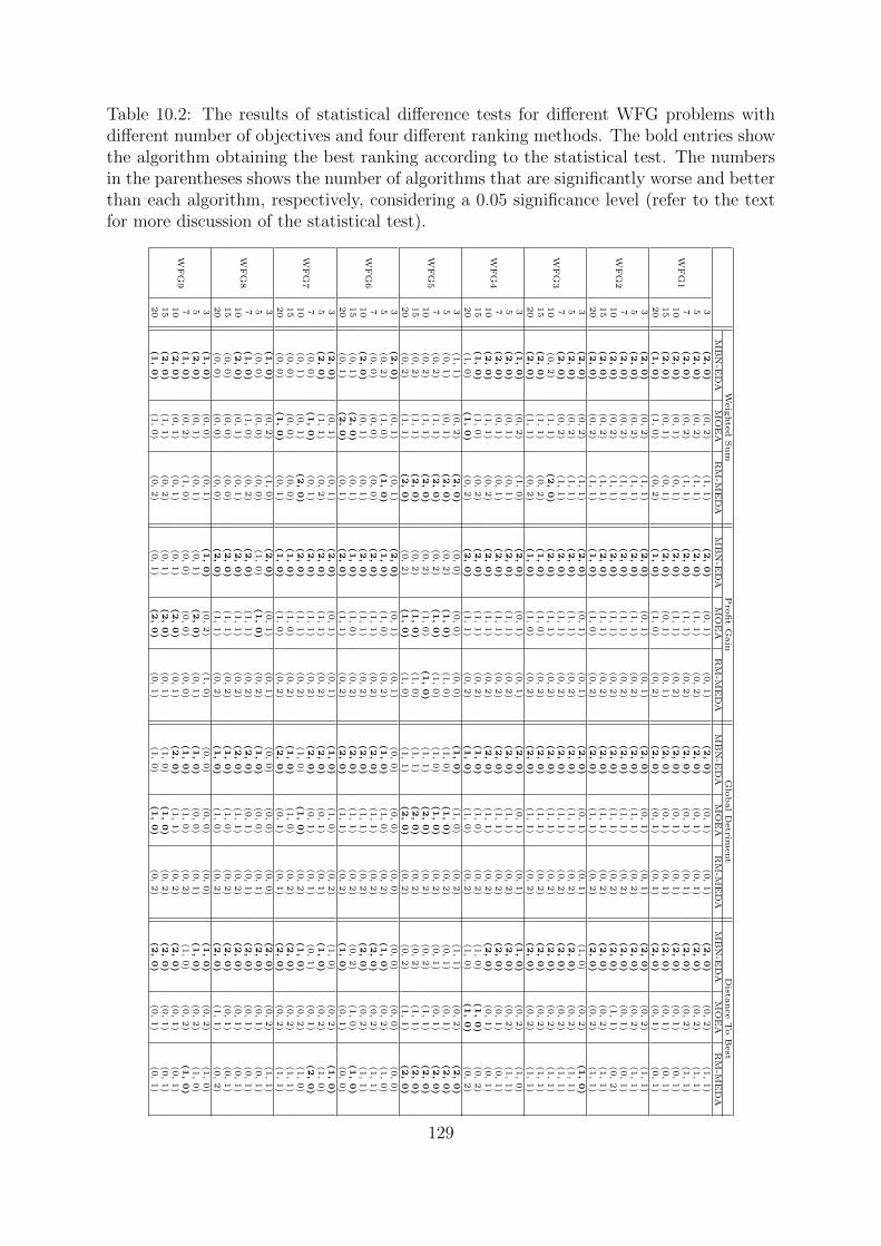
Table 10.2: The results of statistical difference tests for different WFG problems withdifferent number of objectives and four different ranking methods. The bold entries showthe algorithm obtaining the best ranking according to the statistical test. The numbersin the parentheses shows the number of algorithms that are significantly worse and betterthan each algorithm, respectively, considering a 0.05 significance level (refer to the textfor more discussion of the statistical test).

Weig

hte

dSum

Pro

fit

Gain

Glo

bal

Detrim

ent

Dista

nce

To

Best

MB

N-E

DA

MO

EA

RM

-ME

DA

MB

N-E

DA

MO

EA

RM

-ME

DA

MB

N-E

DA

MO

EA

RM

-ME

DA

MB

N-E

DA

MO

EA

RM

-ME

DA

WF

G1

3(2,0)

(0,

2)

(1,

1)

(2,0)

(0,

1)

(0,

1)

(2,0)

(0,

1)

(0,

1)

(2,0)

(0,

2)

(1,

1)

5(2,0)

(0,

2)

(1,

1)

(2,0)

(1,

1)

(0,

2)

(2,0)

(0,

1)

(0,

1)

(2,0)

(0,

2)

(1,

1)

7(2,0)

(0,

2)

(1,

1)

(2,0)

(1,

1)

(0,

2)

(2,0)

(0,

1)

(0,

1)

(2,0)

(0,

2)

(1,

1)

10

(2,0)

(0,

1)

(0,

1)

(2,0)

(1,

1)

(0,

2)

(2,0)

(0,

1)

(0,

1)

(2,0)

(0,

1)

(0,

1)

15

(2,0)

(0,

1)

(0,

1)

(2,0)

(0,

1)

(0,

1)

(2,0)

(0,

1)

(0,

1)

(2,0)

(0,

1)

(0,

1)

20

(1,0)

(1,

0)

(0,

2)

(1,0)

(1,

0)

(0,

2)

(2,0)

(0,

1)

(0,

1)

(2,0)

(0,

1)

(0,

1)

WF

G2

3(2,0)

(0,

2)

(1,

1)

(2,0)

(0,

1)

(0,

1)

(2,0)

(0,

1)

(0,

1)

(2,0)

(0,

2)

(1,

1)

5(2,0)

(0,

2)

(1,

1)

(2,0)

(1,

1)

(0,

2)

(2,0)

(1,

1)

(0,

2)

(2,0)

(0,

2)

(1,

1)

7(2,0)

(0,

2)

(1,

1)

(2,0)

(1,

1)

(0,

2)

(2,0)

(1,

1)

(0,

2)

(2,0)

(0,

1)

(0,

1)

10

(2,0)

(0,

2)

(1,

1)

(2,0)

(1,

1)

(0,

2)

(2,0)

(1,

1)

(0,

2)

(2,0)

(1,

1)

(0,

2)

15

(2,0)

(0,

2)

(1,

1)

(2,0)

(1,

1)

(0,

2)

(2,0)

(1,

1)

(0,

2)

(2,0)

(0,

2)

(1,

1)

20

(2,0)

(0,

2)

(1,

1)

(1,0)

(1,

0)

(0,

2)

(2,0)

(1,

1)

(0,

2)

(2,0)

(0,

2)

(1,

1)

WF

G3

3(2,0)

(0,

2)

(1,

1)

(2,0)

(0,

1)

(0,

1)

(2,0)

(0,

1)

(0,

1)

(1,

0)

(0,

2)

(1,0)

5(2,0)

(0,

2)

(1,

1)

(2,0)

(1,

1)

(0,

2)

(2,0)

(1,

1)

(0,

2)

(2,0)

(0,

2)

(1,

1)

7(2,0)

(0,

2)

(1,

1)

(2,0)

(1,

1)

(0,

2)

(2,0)

(1,

1)

(0,

2)

(2,0)

(0,

2)

(1,

1)

10

(0,

2)

(1,

1)

(2,0)

(2,0)

(1,

1)

(0,

2)

(2,0)

(1,

1)

(0,

2)

(2,0)

(0,

2)

(1,

1)

15

(2,0)

(1,

1)

(0,

2)

(1,0)

(1,

0)

(0,

2)

(2,0)

(1,

1)

(0,

2)

(2,0)

(0,

2)

(1,

1)

20

(2,0)

(1,

1)

(0,

2)

(1,0)

(1,

0)

(0,

2)

(2,0)

(1,

1)

(0,

2)

(2,0)

(0,

2)

(1,

1)

WF

G4

3(1,0)

(0,

2)

(1,

0)

(2,0)

(0,

1)

(0,

1)

(2,0)

(0,

1)

(0,

1)

(1,0)

(0,

2)

(1,

0)

5(2,0)

(0,

1)

(0,

1)

(2,0)

(1,

1)

(0,

2)

(2,0)

(1,

1)

(0,

2)

(2,0)

(0,

2)

(1,

1)

7(2,0)

(0,

1)

(0,

1)

(2,0)

(1,

1)

(0,

2)

(2,0)

(1,

1)

(0,

2)

(2,0)

(0,

1)

(0,

1)

10

(2,0)

(1,

1)

(0,

2)

(2,0)

(1,

1)

(0,

2)

(2,0)

(1,

1)

(0,

2)

(2,0)

(0,

1)

(0,

1)

15

(1,0)

(1,

0)

(0,

2)

(2,0)

(1,

1)

(0,

2)

(1,0)

(1,

0)

(0,

2)

(1,

0)

(1,0)

(0,

2)

20

(1,

0)

(1,0)

(0,

2)

(2,0)

(1,

1)

(0,

2)

(1,0)

(1,

0)

(0,

2)

(1,

0)

(1,0)

(0,

2)

WF

G5

3(1

,1)

(0,

2)

(2,0)

(0,

0)

(0,

0)

(0,

0)

(1,0)

(1,

0)

(0,

2)

(1,

1)

(0,

2)

(2,0)

5(0

,1)

(0,

1)

(2,0)

(0,

2)

(1,0)

(1,

0)

(1,

0)

(1,0)

(0,

2)

(0,

1)

(0,

1)

(2,0)

7(0

,2)

(1,

1)

(2,0)

(0,

2)

(1,0)

(1,

0)

(1,

0)

(1,0)

(0,

2)

(0,

1)

(0,

1)

(2,0)

10

(0,

2)

(1,

1)

(2,0)

(0,

2)

(1,

0)

(1,0)

(1,

1)

(2,0)

(0,

2)

(0,

2)

(1,

1)

(2,0)

15

(0,

2)

(1,

1)

(2,0)

(0,

2)

(1,0)

(1,

0)

(1,

1)

(2,0)

(0,

2)

(0,

2)

(1,

1)

(2,0)

20

(0,

2)

(1,

1)

(2,0)

(0,

2)

(1,0)

(1,

0)

(1,

1)

(2,0)

(0,

2)

(0,

2)

(1,

1)

(2,0)

WF

G6

3(2,0)

(0,

1)

(0,

1)

(2,0)

(0,

1)

(0,

1)

(0,

0)

(0,

0)

(0,

0)

(0,

0)

(0,

0)

(0,

0)

5(0

,2)

(1,

0)

(1,0)

(1,0)

(1,

0)

(0,

2)

(1,0)

(1,

0)

(0,

2)

(1,0)

(0,

2)

(1,

0)

7(0

,0)

(0,

0)

(0,

0)

(2,0)

(1,

1)

(0,

2)

(2,0)

(1,

1)

(0,

2)

(2,0)

(0,

2)

(1,

1)

10

(2,0)

(0,

1)

(0,

1)

(2,0)

(1,

1)

(0,

2)

(2,0)

(1,

1)

(0,

2)

(2,0)

(0,

2)

(1,

1)

15

(0,

1)

(2,0)

(0,

1)

(1,0)

(1,

0)

(0,

2)

(2,0)

(1,

1)

(0,

2)

(0,

2)

(1,

0)

(1,0)

20

(0,

1)

(2,0)

(0,

1)

(2,0)

(1,

1)

(0,

2)

(2,0)

(1,

1)

(0,

2)

(1,0)

(0,

1)

(0,

0)

WF

G7

3(2,0)

(0,

1)

(0,

1)

(2,0)

(0,

1)

(0,

1)

(1,0)

(1,

0)

(0,

2)

(1,

0)

(0,

2)

(1,0)

5(2,0)

(1,

1)

(0,

2)

(2,0)

(1,

1)

(0,

2)

(2,0)

(0,

1)

(0,

1)

(1,0)

(0,

2)

(1,

0)

7(0

,0)

(1,0)

(0,

1)

(2,0)

(1,

1)

(0,

2)

(2,0)

(0,

1)

(0,

1)

(0,

1)

(0,

1)

(2,0)

10

(0,

1)

(0,

1)

(2,0)

(2,0)

(1,

1)

(0,

2)

(1,

0)

(1,0)

(0,

2)

(1,0)

(0,

2)

(1,

0)

15

(0,

0)

(0,

0)

(0,

0)

(1,0)

(1,

0)

(0,

2)

(1,0)

(1,

0)

(0,

2)

(2,0)

(0,

2)

(1,

1)

20

(0,

0)

(1,0)

(0,

1)

(1,0)

(1,

0)

(0,

2)

(2,0)

(0,

1)

(0,

1)

(2,0)

(0,

2)

(1,

1)

WF

G8

3(1,0)

(0,

2)

(1,

0)

(2,0)

(0,

1)

(0,

1)

(0,

0)

(0,

0)

(0,

0)

(2,0)

(0,

2)

(1,

1)

5(0

,0)

(0,

0)

(0,

0)

(1,

0)

(1,0)

(0,

2)

(1,0)

(0,

0)

(0,

1)

(2,0)

(0,

1)

(0,

1)

7(1,0)

(1,

0)

(0,

2)

(2,0)

(1,

1)

(0,

2)

(2,0)

(0,

1)

(0,

1)

(2,0)

(0,

1)

(0,

1)

10

(2,0)

(0,

1)

(0,

1)

(2,0)

(1,

1)

(0,

2)

(2,0)

(1,

1)

(0,

2)

(2,0)

(0,

1)

(0,

1)

15

(0,

0)

(0,

0)

(0,

0)

(2,0)

(1,

1)

(0,

2)

(1,0)

(1,

0)

(0,

2)

(2,0)

(0,

1)

(0,

1)

20

(0,

0)

(0,

0)

(0,

0)

(2,0)

(1,

1)

(0,

2)

(1,0)

(1,

0)

(0,

2)

(2,0)

(1,

1)

(0,

2)

WF

G9

3(1,0)

(0,

0)

(0,

1)

(1,0)

(0,

2)

(1,

0)

(0,

0)

(0,

0)

(0,

0)

(1,0)

(0,

2)

(1,

0)

5(2,0)

(0,

1)

(0,

1)

(0,

1)

(2,0)

(0,

1)

(1,0)

(0,

0)

(0,

1)

(1,0)

(0,

2)

(1,

0)

7(1,0)

(0,

2)

(1,

0)

(0,

0)

(0,

0)

(0,

0)

(1,0)

(1,

0)

(0,

2)

(1,

0)

(0,

2)

(1,0)

10

(2,0)

(0,

1)

(0,

1)

(0,

1)

(2,0)

(0,

1)

(2,0)

(1,

1)

(0,

2)

(2,0)

(0,

1)

(0,

1)

15

(2,0)

(1,

1)

(0,

2)

(0,

1)

(2,0)

(0,

1)

(1,

0)

(1,0)

(0,

2)

(2,0)

(0,

1)

(0,

1)

20

(1,0)

(1,

0)

(0,

2)

(0,

1)

(2,0)

(0,

1)

(1,

0)

(1,0)

(0,

2)

(2,0)

(0,

1)

(0,

1)

129

Table 10.3: Characteristics of the unconstrained MOPs used in CEC09 benchmark.

Name No. Objectives No. Variables F ∗ Size

UF1 2 30 1000

UF2 2 30 1000

UF3 2 30 1000

UF4 2 30 1000

UF5 2 30 21

UF6 2 30 1000

UF7 2 30 1000

UF8 3 30 10000

UF9 3 30 10000

UF10 3 30 10000

DTLZ2 5 30 5000

DTLZ3 5 30 5000

WFG1 5 30 5000

important and can influence its performance. For two- and three-objective MOPs, wehave used the weight vector generation method proposed in the original paper by settingthe number of different weight levels to respectively H = 99 and H = 19, resulting inpopulation sizes of N = 100 and N = 210, respectively. For five-objective MOPs, themethod proposed in [Zhang et al., 2009a] is used to generate a well distributed set ofweight vectors for a population size of N = 300 and a random pool of 15000 weightvectors. The rest of algorithm parameters are set to their default values according to theoriginal paper.

MOEA-HypE belongs to the group of indicator-based EMO algorithms [Zitzler andKunzli, 2004]. These algorithms use the quality indicators values, usually used to evaluatethe final Pareto set approximations, to rank and select solutions in the course of evolution.One of the quality indicators used for this purpose is the hypervolume indicator. Givena Pareto set approximation A, its hypervolume indicator value with respect to a set R ofreference points in the objective space, denoted as Ih(A,R), is given as

Ih(A,R) =⋃x∈A

H(f(x), R), (10.11)

where H(a, B) indicates the (hyper-)volume between point a and the points of set Bin the objective space. A higher value for this indicator implies a better Pareto setapproximation. Computing the hypervolume indicator is very time consuming and itscomputational complexity is exponential in the number of objectives.

To simplify this computation, in MOEA-HypE a set of points are randomly sampledin the objective space and is used to obtain an estimation of the hypervolume dominatedby each solution. These estimated hypervolume values are then used to rank the solutionsand select a subset as parents with a tournament selection strategy (with a tournamentsize of 5) for offspring generation. In the replacement step, population and offspring

130

solutions are aggregated and sorted into a number of Pareto sets, using the non-dominatedsorting algorithm. However, instead of computing the crowding distances of solutionswithin each Pareto set, the estimated hypervolume values of the solutions are used toselect the elite solutions in each set for forming the population of the next generation. Inthis study we use a sample of 10000 points for hypervolume estimation as it is suggestedin the original paper of this algorithm. The rest of algorithm parameters are set to theirdefault values.

Both of these algorithms use the same genetic operators as the ones used in NSGA-II (simulated binary crossover and polynomial mutation) for generating new solutions.However, MOEA-HypE generates N/2 new offspring solutions in each generation, whereasMOEA/D generates N new offspring solutions by evolving all of the solutions in the pop-ulation. This means that during optimization, MOEA/D processes twice the numberof solutions that is searched by MOEA-HypE. Therefore, to have a fair comparison be-tween the algorithms, we impose a similar maximum number of fitness evaluations forboth of the algorithms by setting the population size of MOEA-HypE to twice the sizeof population in MOEA/D.

MBN-EDA is tested with three different ranking methods in these experiments. Fromthe ranking methods introduced in Section 10.3.1, we have selected gDB and gGD. Inorder to extend the diversity of solutions when using gDB, a tournament selection strategysimilar to that used by MOEA-HypE is adopted for this ranking method. In additionto these two ranking methods, MBN-EDA is also tested when using HypE method forranking and selecting the solutions, in order to compare joint modeling in MBN-EDA withgenetic operators in the other two EMO algorithms. Other parameters of MBN-EDA,like population size, are set similar to those in MOEA-HypE.

The quality indicator suggested in CEC09 benchmark for comparing the approximatedfronts is IGD indicator. The size of the sampling set provided for the Pareto optimal frontof each of the MOPs in CEC09 benchmark is shown in Table 10.3. In addition to thisquality indicator, we have also evaluated the approximated Pareto sets with epsilon andhypervolume indicators. The sampling of the Pareto optimal front is also used as thereference set when computing the epsilon indicator. For the hypervolume indicator, apoint in the objective space having the worse values for all of the objective functions,usually referred to as the nadir point, is used as the reference. This point is equally setfor all of the algorithms to 10000 in all of the objective dimensions and for all of theproblems.

Results

Figures 10.8–10.11 show the values of the quality indicators for the final Pareto setsapproximated by each of the algorithms on each of the problems, in 20 independent runs.The maximum number of generations is equally set for all of the algorithms to 300.

The results show that the algorithms have different behaviors on each of the testedMOPs. In general it seems that the problems in CEC09 benchmark are better optimizedwhen using the decomposition method in MOEA/D for guiding the search. With thismethod, each of the subproblems will guide the search into a different subspace of theobjective space, depending on the weight vector which is used for decomposition. There-fore the algorithm is able to search different regions of the objective space even until the

131

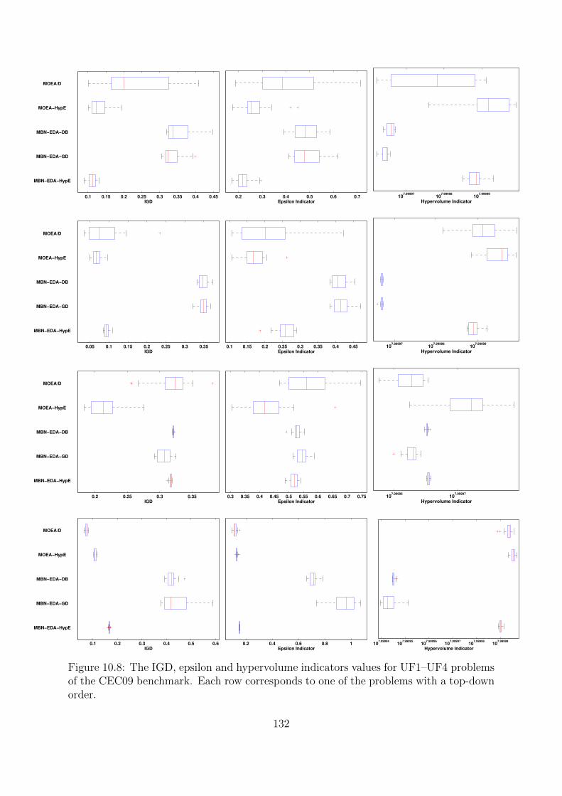
0.1 0.15 0.2 0.25 0.3 0.35 0.4 0.45

MOEA/D

MOEA−HypE

MBN−EDA−DB

MBN−EDA−GD

MBN−EDA−HypE

IGD0.2 0.3 0.4 0.5 0.6 0.7

MOEA/D

MOEA−HypE

MBN−EDA−DB

MBN−EDA−GD

MBN−EDA−HypE

Epsilon Indicator10

7.9999710

7.9999810

7.99999

MOEA/D

MOEA−HypE

MBN−EDA−DB

MBN−EDA−GD

MBN−EDA−HypE

Hypervolume Indicator

0.05 0.1 0.15 0.2 0.25 0.3 0.35

MOEA/D

MOEA−HypE

MBN−EDA−DB

MBN−EDA−GD

MBN−EDA−HypE

IGD0.1 0.15 0.2 0.25 0.3 0.35 0.4 0.45

MOEA/D

MOEA−HypE

MBN−EDA−DB

MBN−EDA−GD

MBN−EDA−HypE

Epsilon Indicator10

7.9999710

7.9999810

7.99999

MOEA/D

MOEA−HypE

MBN−EDA−DB

MBN−EDA−GD

MBN−EDA−HypE

Hypervolume Indicator

0.2 0.25 0.3 0.35

MOEA/D

MOEA−HypE

MBN−EDA−DB

MBN−EDA−GD

MBN−EDA−HypE

IGD0.3 0.35 0.4 0.45 0.5 0.55 0.6 0.65 0.7 0.75

MOEA/D

MOEA−HypE

MBN−EDA−DB

MBN−EDA−GD

MBN−EDA−HypE

Epsilon Indicator10

7.9999610

7.99997

MOEA/D

MOEA−HypE

MBN−EDA−DB

MBN−EDA−GD

MBN−EDA−HypE

Hypervolume Indicator

0.1 0.2 0.3 0.4 0.5 0.6

MOEA/D

MOEA−HypE

MBN−EDA−DB

MBN−EDA−GD

MBN−EDA−HypE

IGD0.2 0.4 0.6 0.8 1

MOEA/D

MOEA−HypE

MBN−EDA−DB

MBN−EDA−GD

MBN−EDA−HypE

Epsilon Indicator10

7.9999410

7.9999510

7.9999610

7.9999710

7.9999810

7.99999

MOEA/D

MOEA−HypE

MBN−EDA−DB

MBN−EDA−GD

MBN−EDA−HypE

Hypervolume Indicator

Figure 10.8: The IGD, epsilon and hypervolume indicators values for UF1–UF4 problemsof the CEC09 benchmark. Each row corresponds to one of the problems with a top-downorder.

132

0.5 1 1.5 2 2.5

MOEA/D

MOEA−HypE

MBN−EDA−DB

MBN−EDA−GD

MBN−EDA−HypE

IGD1 1.5 2 2.5

MOEA/D

MOEA−HypE

MBN−EDA−DB

MBN−EDA−GD

MBN−EDA−HypE

Epsilon Indicator10

7.9998110

7.9998410

7.9998710

7.999910

7.99993

MOEA/D

MOEA−HypE

MBN−EDA−DB

MBN−EDA−GD

MBN−EDA−HypE

Hypervolume Indicator

0.4 0.6 0.8 1 1.2 1.4 1.6

MOEA/D

MOEA−HypE

MBN−EDA−DB

MBN−EDA−GD

MBN−EDA−HypE

IGD0.4 0.6 0.8 1 1.2 1.4 1.6 1.8

MOEA/D

MOEA−HypE

MBN−EDA−DB

MBN−EDA−GD

MBN−EDA−HypE

Epsilon Indicator10

7.9998710

7.9998910

7.9999110

7.9999310

7.9999510

7.99997

MOEA/D

MOEA−HypE

MBN−EDA−DB

MBN−EDA−GD

MBN−EDA−HypE

Hypervolume Indicator

0.1 0.2 0.3 0.4 0.5 0.6 0.7

MOEA/D

MOEA−HypE

MBN−EDA−DB

MBN−EDA−GD

MBN−EDA−HypE

IGD0.2 0.3 0.4 0.5 0.6 0.7 0.8 0.9 1

MOEA/D

MOEA−HypE

MBN−EDA−DB

MBN−EDA−GD

MBN−EDA−HypE

Epsilon Indicator10

7.9999510

7.9999610

7.9999710

7.9999810

7.99999

MOEA/D

MOEA−HypE

MBN−EDA−DB

MBN−EDA−GD

MBN−EDA−HypE

Hypervolume Indicator

0.1 0.2 0.3 0.4 0.5 0.6 0.7 0.8 0.9 1

MOEA/D

MOEA−HypE

MBN−EDA−DB

MBN−EDA−GD

MBN−EDA−HypE

IGD0.3 0.4 0.5 0.6 0.7 0.8 0.9 1

MOEA/D

MOEA−HypE

MBN−EDA−DB

MBN−EDA−GD

MBN−EDA−HypE

Epsilon Indicator10

12

MOEA/D

MOEA−HypE

MBN−EDA−DB

MBN−EDA−GD

MBN−EDA−HypE

Hypervolume Indicator

Figure 10.9: The IGD, epsilon and hypervolume indicators values for UF5–UF8 problemsof the CEC09 benchmark. Each row corresponds to one of the problems with a top-downorder.

133

0.2 0.25 0.3 0.35 0.4 0.45 0.5 0.55 0.6 0.65

MOEA/D

MOEA−HypE

MBN−EDA−DB

MBN−EDA−GD

MBN−EDA−HypE

IGD0.5 0.6 0.7 0.8 0.9 1

MOEA/D

MOEA−HypE

MBN−EDA−DB

MBN−EDA−GD

MBN−EDA−HypE

Epsilon Indicator10

12

MOEA/D

MOEA−HypE

MBN−EDA−DB

MBN−EDA−GD

MBN−EDA−HypE

Hypervolume Indicator

0.5 1 1.5 2 2.5

MOEA/D

MOEA−HypE

MBN−EDA−DB

MBN−EDA−GD

MBN−EDA−HypE

IGD0.6 0.8 1 1.2 1.4 1.6 1.8 2 2.2

MOEA/D

MOEA−HypE

MBN−EDA−DB

MBN−EDA−GD

MBN−EDA−HypE

Epsilon Indicator10

12

MOEA/D

MOEA−HypE

MBN−EDA−DB

MBN−EDA−GD

MBN−EDA−HypE

Hypervolume Indicator

0.2 0.4 0.6 0.8 1 1.2

MOEA/D

MOEA−HypE

MBN−EDA−DB

MBN−EDA−GD

MBN−EDA−HypE

IGD0.4 0.6 0.8 1 1.2 1.4

MOEA/D

MOEA−HypE

MBN−EDA−DB

MBN−EDA−GD

MBN−EDA−HypE

Epsilon Indicator10

19.999710

19.9998

MOEA/D

MOEA−HypE

MBN−EDA−DB

MBN−EDA−GD

MBN−EDA−HypE

Hypervolume Indicator

200 400 600 800 1000 1200 1400 1600 1800

MOEA/D

MOEA−HypE

MBN−EDA−DB

MBN−EDA−GD

MBN−EDA−HypE

IGD200 400 600 800 1000 1200 1400 1600 1800

MOEA/D

MOEA−HypE

MBN−EDA−DB

MBN−EDA−GD

MBN−EDA−HypE

Epsilon Indicator10

20

MOEA/D

MOEA−HypE

MBN−EDA−DB

MBN−EDA−GD

MBN−EDA−HypE

Hypervolume Indicator

Figure 10.10: The IGD, epsilon and hypervolume indicators values for UF9, UF10,DTLZ2 and DTLZ3 problems of the CEC09 benchmark. Each row corresponds to one ofthe problems with a top-down order.

134

2.5 3 3.5 4 4.5 5

MOEA/D

MOEA−HypE

MBN−EDA−DB

MBN−EDA−GD

MBN−EDA−HypE

IGD1 1.5 2 2.5

MOEA/D

MOEA−HypE

MBN−EDA−DB

MBN−EDA−GD

MBN−EDA−HypE

Epsilon Indicator10

19.999710

19.999710

19.999810

19.999810

19.9998

MOEA/D

MOEA−HypE

MBN−EDA−DB

MBN−EDA−GD

MBN−EDA−HypE

Hypervolume Indicator

Figure 10.11: The IGD, epsilon and hypervolume indicators values for WFG1 problemof the CEC09 benchmark.

final stages of the evolution.

However, for some of the MOPs in this benchmark, like UF1, UF3, UF6 and UF7,where the optimal Pareto set and its corresponding optimal Pareto front have almostsimilar geometry, the other dominance-based algorithms are able to obtain better approx-imations of the Pareto optimal front. Especially on problems UF1 and UF7, MOEA/D isoutperformed by the HypE method for solution ranking, whether using genetic operatorsor joint model estimation for generating new solutions. An explanation for this behavioris that using decomposition on some of the MOPs causes the algorithm to miss certaininformation about the promising areas of the search space, thus reducing the effectivenessof this method.

It can be observed that the overall performance of MBN-EDA with HypE selectionmethod is superior to the performance observed with the other two ranking methods,according to the values of quality indicators. This suggests that the hypervolume indica-tor estimation provides a better solution ranking than gDB and gGD methods. A closerlook at the quality of the approximated fronts along different generations of the evolutionhas also revealed that HypE is less affected by the specific geometry of the search space.Again, there are some problem instances like UF5, UF6 and UF10 for which gDB pro-vides a better solution ranking than HypE, resulting in better Pareto set approximationsaccording to the indicator values.

The comparison between MOEA-HypE and MBN-EDA-HypE indicates that for someof the tested MOPs like UF1, UF8, DTLZ2 and WFG1, which cover MOPs with differentnumber of objectives, the Pareto sets approximated by MBN-EDA-HypE are better ac-cording to the indicator values. Since both of these algorithms are using similar selectionmethods, this improvement in the results can be directly attributed to the better solutionsearch in MBN-EDA with its joint modeling of variables and objectives. Our investiga-tion of the populations evolved in MOEA-HypE and MBN-EDA-HypE suggests that jointmodeling in MBN-EDA allows the algorithm to rapidly improve its approximated frontin early generations of the search, whereas with the genetic operators in MOEA-HypEusually the improvement of the approximated front is slower. However, the diversity ofthe population in MBN-EDA may not be preserved very well during evolution and thealgorithm can enter a stagnation state. On the other hand, with genetic operators inMOEA-HypE more diverse populations are generated during search and except for some

135

of the MOPs, the algorithm can constantly improve its approximated front.A point that should be noted here is that when HypE selection method is used, the

algorithms are directly optimizing the hypervolume indicator. Thus, using the same in-dicator to evaluate their achieved results may not properly reflect their performances,especially because the hypervolume indicator may overrate certain regions of the ap-proximated fronts [Zitzler and Thiele, 1999]. For the algorithms with HypE selectionmethod, the results provided by IGD and epsilon indicators are a better reference oftheir performance.

10.6 Problem Structure Estimation

One of the advantages of EDAs is that apart from finding solutions to the optimiza-tion problem, they estimate a probabilistic model which captures certain regularities ofthe problem search space and are common among the solutions. This kind of meta in-formation is especially useful when the intrinsic properties of the problem at hand areunknown in advance. Especially, in multi-objective optimization, the estimated modelencodes common properties of the approximated Pareto set which, in decision making,can be used together or even instead of the non-dominated solutions, e.g. when the sizeof the approximated Pareto set is very large.

Recently, several works have studied the use of data mining techniques to obtainnew knowledge from the approximated Pareto sets in EMO algorithms after optimization[Bandaru and Deb, 2011; Deb et al., 2012]. However, multi-objective EDAs already obtainthis kind of information during optimization, depending on the probabilistic model theyuse. Specifically, the type of joint modeling of both variables and objectives used inMBN-EDA offers a systematic way for estimating the structure of an MOP.

A major concern of our study in this chapter is to analyze the MOP structures esti-mated by MBN-EDA in the course of evolution. These structures are important not onlybecause they can improve optimization by providing information about different typesof (in)dependencies existing in the problem, but also because they can give DMs morecontrol over the selection of the desired information from the Pareto set approximations[Ulrich et al., 2008], and better insight into how different variables influence the objec-tives or the way objectives interact [Chan and Chung, 2004]. To examine MBN-EDA’sability to retrieve the MOP structure, we have analyzed the structures estimated forWFG1 problem with five objectives and 16 variables in a number of different case stud-ies. To include the factor of different training data used for estimating MOP structure inthe analysis, MBN-EDA is tested with two of the ranking methods described in Section10.3.1 in this study, namely gPG and gDB.

Selection of Relevant Variables

In the first case study, nine irrelevant variables are added to the problem and uniformlydistributed among other variables. These variables do not affect the outcome of objectivefunctions of the MOP. Figure 10.12 shows the absolute weight of the links encoded inMBN’s bridge substructure between objectives and variables along the evolution path ofMBN-EDA. The weights are averaged over 20 independent runs. We can see that MBN-EDA is able to clearly distinguish between relevant and irrelevant variables in the studied

136

0 50 100 150 200 250 3000

0.005

0.01

0.015

0.02

0.025

0.03

0.035Distance to best ordering

Generations

Avg

. w

eig

ht

of

arc

s

To relevant variables

To irrelevant variables

0 50 100 150 200 250 3000

0.005

0.01

0.015

0.02

0.025

0.03

0.035Profit of gain ordering

Generations

Av

g.

we

igh

t o

f a

rcs

Figure 10.12: The average weight of the links from objectives to variables in the 5-objective WFG1 problem which includes irrelevant variables.

MOP. The low weight of the links between objectives and irrelevant variables in theestimated MBNs is either because the objectives and these variables have been encoded asconditionally independent given other variables and objectives, or any existing link has avery small weight, allowing the algorithm to bypass the noise introduced by these variablesto the problem. Although the models are estimated from different initial populations inthe each of the runs, the structural information encoded between objectives and variablesis very similar. It is also shown that the populations selected according to the gPG rankingmethod help to better distinguish between relevant and irrelevant variables especially inthe final generations where the algorithm focuses on specific regions of the search space.

Identifying Redundant Objectives

The second case study analyzes the structures estimated for an eight-objective WFG1problem with three pairs of similar objectives. Figure 10.13 compares the absolute weightof the arcs between similar objectives with those between dissimilar objective pairs, en-coded in the class substructure of MBN in different generations of MBN-EDA. The resultsare averaged over 20 independent runs. The relatively high weights between similar ob-jectives show that MBN-EDA is correctly encoding a strong dependency between theseobjectives compared with the other relationships in the class subgraph. Note that a closerinspection of the models estimated in different runs with different initial populations hasrevealed that such a dependency between similar objectives is encoded in the modelsestimated in all of the runs. We can also see that the information about the similarity ofobjectives in the MBN’s class subgraph is better captured from the populations selectedaccording to the gDB ranking method.

Estimated Structures

Based on the observations from the above two case studies, the third case study di-rectly inspects the structures estimated by MBN-EDA for the WFG1 problem. In the5-objective WFG1 problem considered in this section, the number of position variables isset to k = 4 and the number of distance variables is set to l = 12 (see Section 9.4.1). A

137

0 50 100 150 200 250 3000

0.05

0.1

0.15

0.2

0.25

0.3

0.35

0.4

0.45

0.5Distance to best ordering

Generations

Avg

. w

eig

ht

of

arc

s

0 50 100 150 200 250 3000

0.05

0.1

0.15

0.2

0.25

0.3

0.35

0.4

0.45

0.5Profit of gain ordering

Generations

Avg

. w

eig

ht

of

arc

s

To similar objectives

To dissimilar objectives

Figure 10.13: The average weight of the links between objectives in the 8-objective WFG1problem with three pairs of similar objectives.

simplified definition of the five objective functions in this problem can be given as follows[Huband et al., 2006]:

f1(x) = a+ 2 · h1

(g2(x1), g2(x2), g2(x3), g2(x4)

)f2(x) = a+ 4 · h2

(g2(x1), g2(x2), g2(x3), g2(x4)

)f3(x) = a+ 6 · h3

(g2(x1), g2(x2), g2(x3)

)(10.12)

f4(x) = a+ 8 · h4

(g2(x1), g2(x2)

)f5(x) = a+ 10 · h5

(g2(x1)

),

where a = g1(x5, . . . , x16), and g1(·) and g2(·) represent a composition of transformationfunctions on the input variables.

Figure 10.14 shows part of the structures learnt for this problem, consisting of thesignificant arcs and their corresponding nodes with an average absolute weight valuegreater than a threshold set to w ≥ 0.1 (constituting about 7% of the most significantarcs). While there are many links capturing the obscure relationships between variables(not depicted here), it is evident that MBN-EDA attaches more importance to the linksbetween objectives in the class subgraph, and between the objectives and the first fourvariables in the bridge subgraph. Moreover, these dependencies conform to the functiondefinitions given in Equation (10.12). For example, the link between objective nodes Q2

and Q4, which is captured using both of the tested ranking methods, is supported bythe fact that h2(·) is actually a multiplication of h4(·) and two other factors obtainedfrom variables X3 and X4. Another example is the relationship between objective nodeQ1 and the nodes corresponding to the first four variables, either directly or through therelationships with other objectives, since all of these variables influence the value of thefirst objective function.

An important point to note here is the significance of the information provided by thedependencies between objectives, and between objectives and variables in multi-objectiveoptimization from MBN-EDA point of view. There are some studies in the literaturethat analyze how the dependencies between variables are represented in probabilisticmodels [Santana et al., 2009a]. But, to the best of our knowledge, the importance of

138

(a) Distance to best ordering (b) Profit of gain ordering

Figure 10.14: Part of the structure learnt for the 5-objective WFG1 problem showing themost significant edges and their corresponding nodes.

the interactions involving objectives have not been considered so far in other EDAs usedfor multi-objective optimization. Such dependencies allow the proposed MBN-EDA toapproximate how the variables can affect objective values, which is used to generate newsolutions with better objective values.

10.7 Conclusions

The similarity between multi-dimensional classification and multi-objective optimizationmotivates the use of MBNs in the context of EDAs to solve MOPs. A new modelingapproach in multi-objective EDAs was proposed that uses MBN estimation to learn ajoint model of objectives and variables while at the same time distinguishes their rolein the model. The estimated joint model encodes three types of relationships betweenvariables and objectives in three different substructures.

The proposed joint modeling was coupled with different ranking methods introducedin the literature for many-objective optimization and tested on two sets of benchmarkproblems with different number of objectives. The exhaustive experiments comparingMBN-EDA with several state-of-the-art EMO algorithms show promising performancewhen using the proposed joint modeling for guiding the search in the space of candidatesolutions. According to the epsilon quality indicator and compared with a standard EMOalgorithm and a competitive EDA, MBN-EDA was able to obtain significantly betterapproximations of the Pareto set for many of the WFG problems, with a significancelevel of α = 0.05. We found that the choice of ranking methods has a major influenceon the performance of the algorithms for some of the MOPs, as they determine thepopulation used for model estimation and offspring generation. The results also show thatthe proposed MBN-EDA was unable to satisfactorily deal with some MOP properties,like deception in the objective values. The results of the second set of experiments on theCEC09 unconstrained problems show that on some of the MOPs in this benchmark, thejoint modeling in MBN-EDA allows to find considerably better fronts according to threedifferent quality indicators.

139

The proposed joint modeling approach also obtains the MOP structure which can beused for decision making. An analysis of the structures estimated by MBN-EDA along theevolution path showed that the proposed algorithm is able to distinguish between relevantand irrelevant variables, performing a type of variable selection for the objectives encodedin the model. It can also capture stronger dependencies between similar objectives whichhelps to identify redundant objective functions. The analysis of the specific structuresestimated for the 5-objective WFG1 problem shows that MBN-EDA is able to obtain avery good approximation of this MOP structure. We saw that the information provided bythe relationships between variables and objectives and the inter-objectives dependencies,the two types of interactions completely overlooked by other EDAs, can be very importantfor multi-objective optimization.

140

Chapter 11

Interval-Based Ranking in NoisyEvolutionary Multi-ObjectiveOptimization

11.1 Introduction

A feature of many real-world problems is the existence of noise, which can appear asvariable or environmental change, or/and as uncertainty in the objective values. WhenEMO algorithms based on Pareto dominance relation are used for solving these problems,the noise in objective values can mislead the algorithm by selecting inferior solutions thatare considered good because of noise, and discarding good solutions that are necessaryfor directing the search to promising areas.

One of the ways to deal with noisy objectives is to assume each objective returnsan interval of values for a solution. This interval can be obtained by considering therange of error or amount of noise in the system, or from a set of values obtained frommultiple reevaluations of a solution in different conditions. Considering an interval ofvalues instead of a single value allows the EMO algorithm to take into account the extentof noise in the objectives when selecting solutions for recombination.

In this chapter we present a new solution ranking, called α-degree Pareto dominance,for EMO algorithms applied to noisy problems when objective functions return intervals.This new relation for ranking the solutions allows the intervals to overlap each other,and determines the dominance among solutions based on the extent to which their corre-sponding intervals are better than other solutions. The method can also be extended tothe case where only some of the objective functions of the MOP at hand are noisy. Thissolution ranking method is then integrated into MBN-EDA, proposed in Chapter 10, formulti-objective optimization of noisy MOPs by adapting the joint variable-objective mod-eling method of the algorithm. The contents of this chapter are taken from [Karshenaset al., 2013a].

141

11.2 A Survey of Evolutionary Multi-Objective Op-

timization with Noise

The topic of EMO under uncertainty and noise has recently gained a lot of attention, andmany studies and methods are reported in the literature. In general, as explained by Jinand Branke [2005], three different types of noise handling can be identified in EAs. First,the population-based search in these algorithms, by itself, implicitly deals with certainlevels of noise in objective values. The average quality of a population or subgroups ofthe population, presenting certain subspaces, is less susceptible to noise. Therefore, thelarger the population is, the better the algorithm can overcome the noise in the quality ofsolutions for finding the optimal solutions. However, the existence of several objectivesin a multi-objective scenario reduces the effectiveness of EAs in noise handling [Tan andGoh, 2008]. Second approach is to explicitly reevaluate each solution of the populationseveral times to obtain a better estimation of its objective values. Although this approachgreatly increases the computational cost of optimization, for some of the problems wherethe objective values are obtained as the result of simulations, it is inevitable. A thirdapproach is to consider the noise in objective values in the selection step of EAs. This isusually done by modifying the solution ranking method, assuming a level of uncertaintyin the objective values.

As explained before, noise can exist in the values of the input variables, the outputsof the objective functions or even both. There are some works on EMO algorithmsconsidering the former type of noise, i.e. noise in the input values, which is sometimesreferred to as robust optimization and its aim is to find solutions with the highest stabilityin their objective values. Soares et al. [2009] optimized the worst noisy objective values ofthe solutions (in a min-max formulation) using interval analysis. To decrease the amountof uncertainty in the intervals they propose to recursively divide the intervals into halves,resulting in a grid which is placed on the objective space and is used to compute the worstobjective values of the solutions. The grid also serves as a niching method, penalizingthe solutions that are very close in the objective space. The noise is introduced in theinput variables using an uncertainty vector which is incorporated in the definition of theobjective functions. Goh et al. [2010] offered a classification of the noisy MOPs dependingon the effect of noise on the Pareto front, Pareto set and landscape of the problem. Basedon this classification, they proposed some guidelines for designing challenging MOPs forrobust optimization, and introduced a Gaussian landscape generator using a number ofbasis functions for this purpose.

Most of the algorithms proposed for EMO in noisy environments consider the secondtype of noise, i.e. noise in the objective values, since this type of noise is harder to dealwith. In this type of MOPs it is usually assumed that the objective values are distortedby an additive noise value. Almost all EMO algorithms reviewed in this section considera Gaussian noise model for the objective values of the tested MOPs, unless otherwisementioned.

One of the earliest and well-known approaches to deal with noisy objectives whencomparing two solutions in multi-objective optimization is to use probabilistic dominance,considering the probability that one solution dominates another [Teich, 2001; Hughes,2001]. This approach has been successfully used for optimization in some of the realworld problems like designing the shape of acoustic noise attenuation barriers with several

142

receiver points [Greiner et al., 2009]. Since this method is considered as a main referencein many later works on noisy objectives, we explain here it in more detail.

Definition 11.1. (Dominance Probability) [Teich, 2001; Hughes, 2001] LetU = f(x) and V = f(y) be two vectors of random variables representing the objectivevalues returned for two solutions x and y of a noisy MOP in decision space D. Then theprobability that x dominates y is given by:

P (x ≺ y) =

∫ ∞−∞· · ·∫ ∞−∞

ρU (t)(1−ΨV (t)

)dt, (11.1)

where ρU (·) denotes the joint probability distribution for the output of objective functionsgiven solution x, and ΨV (·) is the cumulative probability distribution for the output ofobjective functions given solution y.

Based on the probability of dominance, ranking strategies like the mean dominanceprobability [Teich, 2001] is used to order the solutions with noisy objective values. Hughes[2001] also tested this approach when the noise is introduced to the input values, showingthe ability of this method for handling noise in both input variables and output ob-jective functions. Bui et al. [2005a] adopted probabilistic dominance in NSGA-II [Debet al., 2002a] and compared it with a version of this algorithm which is based only onreevaluation of objectives. They also proposed a fitness inheritance method to reducethe complexity of reevaluating the objectives. In a separate work [Bui et al., 2005b] theyperformed a comparative study of the noise handling capability of the original versionsof NSGA-II and SPEA2 [Zitzler et al., 2001] in the presence of different noise levels,using several performance measures. Fieldsend and Everson [2005] proposed a Bayesianmethod for obtaining an estimation of the Gaussian noise variance when computing theprobability of dominance between two solutions. They considered different scenarios likeunknown, constant and variable noise for the objective values.

Many of the EMO algorithms proposed for noise handling try to extend the existingsolution ranking and selection methods by considering noise in the values of the objectives.Buche et al. [2002] proposed a noise-tolerant EA using the Pareto strengths-based solutionranking method [Zitzler and Thiele, 1999] assigning a lifetime (number of generations)to the solutions in the archive depending on their strengths. This lifetime is used todetermine which solutions are to be reevaluated or to be used for updating the archive inorder to limit the influence of noisy objective values and outliers. They claim that elitismdoes not necessarily result in faster convergence when noise is present in multi-objectiveoptimization. The proposed algorithm is applied to find an optimal flow of fuel in theburner of a gas turbines.

Babbar et al. [2003] modified NSGA-II to include neighbors of the non-dominatedsolutions in the first Pareto front. Neighboring solutions are determined using the meanand variance of the objective values for each solution, estimated from the reevaluation ofthe solutions. Solutions that are reevaluated less than a predetermined number of timesduring the evolution are considered as outliers and removed from the final Pareto set.Goh and Tan [2007] proposed three techniques for noise handling in an EMO algorithmwhich uses a two-part, discrete-continuous, representation for the solutions. The firsttechnique consists of incorporating the direction of population movement along evolutioninto the generation of new solutions. The second technique is stretching or shrinking

143

the search domain of each variable depending on the behavior of the algorithm in thecurrent phase of evolution. The third technique is to assume objective values are givenas fuzzy numbers and then use two newly proposed dominance relations, called necessityand necessity-possibility, to update the archive of non-dominated solutions maintainedby the algorithm.

Eskandari and Geiger [2009] considered the expected values of the objective functionsand proposed the stochastic dominance relation for ranking the solutions. In the selectionprocess, the solutions are divided into two sets depending on whether they are stochas-tically dominated. The set of stochastically dominated solutions are further ordered byconsidering the expected strength of each solution depending on both how many solutionsit dominates and by how many solutions it is dominated. To detect the algorithm conver-gence in noisy environments they proposed to monitor the rate of hypervolume indicatorgrowth. Bui et al. [2009] proposed the use of adaptive non-overlapping hyper-sphereswhich are locally moved in the search space to reduce the effect of noise. The motivationis that the average objective values of the solutions in a neighborhood of the search spaceprovide a better approximation of the direction of movement during evolution. A PSOinspired algorithm is used to update the center and radius of the hyper-spheres in thesearch space. The algorithm also deploys an archive of solutions and its correspondinghyper-sphere to represent the global behavior of the population.

Syberfeldt et al. [2010] proposed a method to increase the efficiency of solution reevalu-ations. When comparing two solutions in the non-dominated sorting algorithm [Deb et al.,2002a], if the confidence in the differences between their objective values are less than aspecific level, then one of them is reevaluated more to increase the level of confidence.Different Pareto sets are assigned different values of minimum confidence level, and sinceduring evolution the rank of solutions in the population changes, implicit dynamism isintroduced during evolution as each solution is reevaluated. The proposed method is alsoapplied to two real-world problem related to optimization in engine manufacturing lines.Instead of discarding old evaluations of a solution in a noisy problem, Park and Ryu[2011] proposed an accumulating approach which combines old evaluations with the newreevaluation of a solution to improve the expected value estimation of objective functions.

Another approach taken by some of the proposed methods is to use DM providedinformation for EMO in the presence of noise. Mehnen et al. [2007] used desirabilityfunctions to include both the preferences of DM and to reduce the effect of noise. Insteadof performing the search in the objective space, they optimize the expected value ofthe desirability functions computed from noisy objectives. The final Pareto front isobtained by either applying the inverse desirability functions on the approximated frontor computing the objective values of the final Pareto set. The method is used to findthe working parameters of an industrial cutting tool. Wozniak [2007] proposed to usea number of reference points provided by DM, each accompanied with a weight vectorshowing the importance of the objectives, to select fitter solutions in the search process.To maintain the population diversity only one of the solutions in each neighborhood,defined by a predefined neighborhood radius, is selected. The method then is applied forthe design of a motor speed controller.

In addition to the noise in objective values, Kaji et al. [2009] studied the effect of noisein constraint functions of a constrained MOP, trying to reduce the number of infeasiblesolutions selected in the Pareto set. For this purpose they form a history of solutions

144

Table 11.1: Summary of the EMO methods for noisy environments.

Method Noise Type Place of Noise

[Teich, 2001] Probabilistic Dominance Uniform Output

[Hughes, 2001] Probabilistic Dominance Gaussian Input, Output

[Buche et al., 2002] Lifetime-Based Archiving Gaussian Output

[Babbar et al., 2003] Objective Space Neighborhood Gaussian Output

[Bui et al., 2005a] Fitness Inheritance in Reevaluations Gaussian Output

[Fieldsend andEverson, 2005]

Noise Variance Estimation Gaussian Output

[Basseur and Zitzler,2006]

Indicator Value Estimation Uniform Input, Output

[Goh and Tan, 2007]Necessity and Necessity-PossibilityDominance

Gaussian Output

[Mehnen et al., 2007] Desirability Functions Optimization Gaussian Output

[Wozniak, 2007] Weighted Reference Points Gaussian Output

[Boonma and Suzuki,2009]

Confidence-Based SolutionComparison

Gaussian,Uniform,Poisson

Output

[Bui et al., 2009] Search Space Neighborhood Gaussian Output

[Eskandari and Geiger,2009]

Stochastic Dominance Gaussian Output

[Kaji et al., 2009]Value Estimation with LocallyWeighted Ridge Regression

GaussianOutput,Constraints

[Soares et al., 2009] Worst-Case Analysis Gaussian Output

[Syberfeldt et al., 2010] Confidence-Based Reevaluations Gaussian Output

[Park and Ryu, 2011] Reevaluation Accumulation Gaussian Output

and estimate the value of objective and constraint functions by a locally weighted ridgeregression of second order. The weights are defined using a Gaussian kernel. A safetymargin is also introduced to the constraint functions and dynamically adjusted dependingon the variance of the estimated constraint values.

Basseur and Zitzler [2006] proposed an indicator-based EMO algorithm for noisy en-vironments, considering the presence of noise in both the objective functions and theinput variables. They proposed methods to estimate the expected value of the epsilonindicator for ranking the solutions. A uniform noise is assumed for both inputs and out-puts. Boonma and Suzuki [2009] considered different types of distributions like Gaussian,uniform and Poisson for the noise model. Assuming that the quality of each solution isrepresented with several reevaluations of its objectives, they used a support vector ma-chine to determine the confidence level in these objective values. The coverage metric isused to determine the dominance between two solutions after their values are classified asstatistically reliable. The confidence level for accepting the objective values of the solu-tions is dynamically adjusted during evolution according to the disorder among objectivevalues, which is computed with an entropy-based function.

Table 11.1 summarizes the reviewed algorithms.

145

11.3 α-Degree Pareto Dominance

Most of the methods reviewed in the previous section for handling the noise when select-ing a subset of solutions, only consider singular objective values. Although these singularvalues maybe obtained as the result of averaging over several reevaluations, they still donot directly take into account the extent of the noise in the values. We also saw thatsome of the proposed methods optimize the expected values of the objectives and considerthe variance of the objective values, implicitly assuming a type of confidence interval forthe objective values. A closely related approach is the possibilistic dominance method[Goh and Tan, 2007], where objective values are considered to be fuzzy numbers. In thissection we propose a method for directly comparing any kind of intervals, not necessar-ily confidence intervals, which also takes into account interval widths (representing theamount of noise). Moreover, the proposed method can deal with MOPs consisting ofboth singular and interval objectives.

One way to deal with the noise in an MOP when the objective values are representedwith intervals is to extend the Pareto dominance definition (Definition 8.1). In the fol-lowing definitions we assume that the set of objectives F is partitioned into two disjointsubsets of objectives with singular values FS, and noisy objectives with interval valuesFI , such that FS ∪ FI = F and FS ∩ FI = ∅.

Definition 11.2. (Extended Pareto Dominance) Let⌊fj(x)

⌋and

⌈fj(x)

⌉respec-

tively represent the lower and upper bounds of the interval value returned for solution x ∈D, by the noisy objective function fj ∈ FI , i.e. Uj lies in the interval

[⌊fj(x)

⌋,⌈fj(x)

⌉].

Then, solution x is said to strictly dominate solution y, denoted as x ≺e y, if and onlyif:

1. ∀fj ∈ FS fj(x) ≤ fj(y), and

2. ∀fj ∈ FI⌈fj(x)

⌉≤⌊fj(y)

⌋, and

3.(∃fk ∈ FS fk(x) < fk(y) or ∃fk ∈ FI

⌈fk(x)

⌉<⌊fk(y)

⌋).

This definition treats interval values similar to the way it considers singular valuesand only allows a solution to dominate other solutions if its corresponding interval values,returned by noisy objective functions, are strictly better than those of other solutions. Inreal-world noisy MOPs, such a requirement is hardly satisfied. A further extension is torelax this strict requirement and allow the intervals to have some degree of overlapping.

Definition 11.3. (α-Degree Pareto Dominance) Assume the same notations as thoseof Definition 11.2. Then, solution x is said to dominate another solution y with a degreeα ∈ (0, 1], denoted as x ≺α y, if and only if:

1. ∀fj ∈ FS fj(x) ≤ fj(y), and

2. ∀fj ∈ FI degj(x,y) ≥ α, and

3.(∃fk ∈ FS fk(x) < fk(y) ∨ ∃fk ∈ FI degk(x,y) > α

),

146

fj(x)

fj(y)

(a) degj(x,y) = 1

fj(x)

fj(y)

(b) degj(x,y) = 0.75

fj(x)

fj(y)

(c) degj(x,y) = 0.5

fj(x)

fj(y)

(d) degj(x,y) = 0

Figure 11.1: Examples of interval values and the resulting degrees of dominance.

where degj(·, ·) gives the degree that a solution dominates another with respect to the noisyobjective function fj ∈ FI

degj(x,y) = min{

1,max{0,⌊fj(y)

⌋−⌊fj(x)

⌋⌈fj(x)

⌉−⌊fj(x)

⌋}}. (11.2)

Intuitively, degj(x,y) computes the percentage of the interval obtained for solution xthat is not overlapped by the interval obtained for solution y in objective fj ∈ FI . Thus,only the segment in the interval obtained for solution x that is better than the best pointin the interval obtained for solution y (i.e. its lower bound, when minimizing objectives)is taken into account. If α = 1, then Definition 11.3 is reduced to Definition 11.2.Definition 11.3 allows a solution to dominate other solutions when its correspondinginterval values are partially better than those of other solutions.

11.3.1 Discussion

Figure 11.1 shows some examples of possible placements of two intervals and the corre-sponding values of the degj(·, ·) function. With higher values of α, a solution can onlydominate other solutions if a major part of its corresponding interval values are betterthan the best points of the interval values corresponding to other solutions. Thus, highervalues of α place a stricter condition for accepting a solution as non-dominated.

Proposition 11.1. α-degree Pareto dominance defines a partial relation, i.e. with ir-reflexivity, antisymmetry and transitivy properties, on the space of candidate solutions.

147

Proof. Since no x ∈ D exists that satisfies x ≺α x for any α ∈ (0, 1], the relation isirreflexive. To see the antisymmetry of the relation, assume x ≺α y. If ∃fj ∈ FS suchthat fj(x) < fj(y) then y ⊀α x. If ∃fj ∈ FI such that degj(x,y) > α, then by definitionof degj(·, ·) in Equation (11.2) if degj(x,y) > 0 then degj(y,x) = 0 and therefore y ⊀α xfor any α ∈ (0, 1].

For transitivity, assume that x ≺α y and y ≺α z. Then we have ∀fj ∈ FS, fj(x) ≤fj(y) and fj(y) ≤ fj(z). Therefore, fj(x) ≤ fj(z), ∀fj ∈ FS. Similarly, we havedegj(x, z) ≥ α, ∀fj ∈ FI , because if ∀fj ∈ FI such that

⌊fj(x)

⌋<⌊fj(y)

⌋and

⌊fj(y)

⌋<⌊

fj(z)⌋, then we have

⌊fj(x)

⌋<⌊fj(z)

⌋, ∀fj ∈ FI . Now, given either ∃fj ∈ FS such

that fj(x) < fj(y) or ∃fj ∈ FI such that degj(x,y) > α (similarly ∃fj ∈ FS such thatfj(y) < fj(z) or ∃fj ∈ FI such that degj(y, z) > α) we can respectively conclude either∃fj ∈ FS such that fj(x) < fj(z) or ∃fj ∈ FI such that degj(x, z) > α, which completesthe proof of proposition. �

The partial relation defined by α-degree Pareto dominance allows to readily adopt theterms of α-degree Pareto optimal solution, α-degree Pareto optimal set, α-degree Paretooptimal front and α-degree Pareto non-dominated set for noisy MOPs, in the same waythey are defined using the conventional Pareto dominance relation. The α-degree Paretodominance relation also has interesting properties when different confidence levels areconsidered for the objective values. To see this, lets assume that the values returned bynoisy objective functions for solution x are confidence intervals given in the form of(

E(fj(x)

)− εγ

(fj(x)

), E(fj(x)

)+ εγ

(fj(x)

)),

where E(fj(x)

)represents an estimation of the expected value of the jth objective func-

tion for solution x and

εγ(fj(x)

)= z 1−γ

2σ(fj(x)

)is the half-width [Eskandari and Geiger, 2009] of the confidence interval computed ac-cording to a specific confidence level γ. Here, z(1−γ)/2 denotes the value for whichΦ(Z > z(1−γ)/2) = 1−γ

2, where Φ(Z) is the cumulative standard Gaussian (or t-student)

distribution. σ(fj(x)

)is the estimation for the standard deviation of mean objective

value. With confidence intervals, the definition of degj(x,y) for a noisy objective fj ∈ FIcan be rewritten as

degj(x,y) = min{

1,max{0,

(E(fj(y)

)− E

(fj(x)

))−(εγ(fj(y)

)− εγ

(fj(x)

))2εγ(fj(x)

) }}.

(11.3)According to this definition, the degree that a solution dominates another solution

with respect to a noisy objective fj ∈ FI is determined by the differences in both expectedvalues and half-widths. The following propositions show how the change in the confidencelevel γ or dominance degree α affects the α-degree Pareto dominance relation.

Proposition 11.2. Any reduction in the confidence level of the interval values given bynoisy objective functions in FI does not affect x ≺α y, if for every objective functionfj ∈ FI we have E

(fj(x)

)< E

(fj(y)

).

148

Proof. We only consider noisy objectives in FI here because the change in confidence leveldoes not affect singular values. Let x ≺γα y denote that solution x dominates solution ywith a degree α, when the confidence level in the interval value of all noisy objectives inFI is at least γ.

Assuming x ≺γ1α y implies that

∀fj ∈ FI ,

(E(fj(y)

)− E

(fj(x)

))−(εγ1

(fj(y)

)− εγ1

(fj(x)

))2εγ1

(fj(x)

) ≥ α

⇒E(fj(y)

)− E

(fj(x)

)2z 1−γ1

2σ(fj(x)

) −σ(fj(y)

)− σ

(fj(x)

)2σ(fj(x)

) ≥ α.

Changing the confidence level does not influence the second quotient above. The numera-tor of the first quotient is positive because of the assumption of the proposition and, sincez 1−γ1

2> z 1−γ2

2, ∀γ2 < γ1, this quotient will become larger if confidence level decreases to

γ2. Therefore, for all fj ∈ FI(E(fj(y)

)− E

(fj(x)

))−(εγ2

(fj(y)

)− εγ2

(fj(x)

))2εγ2

(fj(x)

) >(E(fj(y)

)− E

(fj(x)

))−(εγ1

(fj(y)

)− εγ1

(fj(x)

))2εγ1

(fj(x)

) ≥ α,

which means x ≺γ2α y. �

Now, let PSγα denote the α-degree Pareto optimal set imposed by α-degree Paretodominance relation ≺γα, when the confidence level in the interval values returned by thenoisy objectives is at least γ.

Corollary 11.1. If γ2 < γ1, then PSγ2α ⊂ PSγ1

α .

Proof. Assume that there exists a solution y such that y ∈ PSγ2α and y /∈ PSγ1

α . Thismeans that there exists a solution x ∈ PSγ1

α such that x ≺γ1α y. By Proposition 11.2

we know that this implies x ≺γ2α y. But the last relation means that y /∈ PSγ2

α whichcontradicts the hypothesis. �

Proposition 11.3. The α-degree Pareto dominance relation between solutions is pre-served when the dominance degree α is decreased.

Proof. It is trivial since if α2 < α1 then degj(x,y) ≥ α1 implies that degj(x,y) > α2, forany two solutions x, y and every objective function fj ∈ FI . �

Corollary 11.2. If α2 < α1, then PSγα2⊂ PSγα1

.

Proof. The same as the proof for Corollary 11.1. �

149

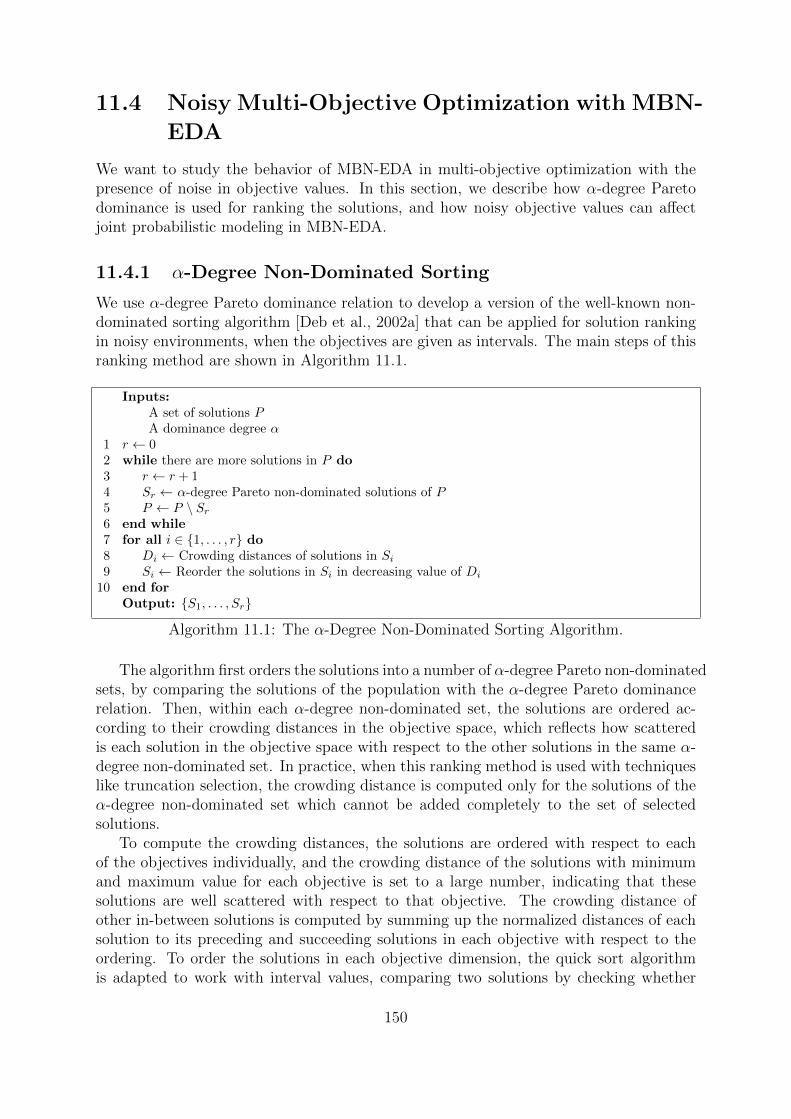
11.4 Noisy Multi-Objective Optimization with MBN-

EDA

We want to study the behavior of MBN-EDA in multi-objective optimization with thepresence of noise in objective values. In this section, we describe how α-degree Paretodominance is used for ranking the solutions, and how noisy objective values can affectjoint probabilistic modeling in MBN-EDA.

11.4.1 α-Degree Non-Dominated Sorting

We use α-degree Pareto dominance relation to develop a version of the well-known non-dominated sorting algorithm [Deb et al., 2002a] that can be applied for solution rankingin noisy environments, when the objectives are given as intervals. The main steps of thisranking method are shown in Algorithm 11.1.

Inputs:A set of solutions PA dominance degree α

1 r ← 02 while there are more solutions in P do3 r ← r + 14 Sr ← α-degree Pareto non-dominated solutions of P5 P ← P \ Sr

6 end while7 for all i ∈ {1, . . . , r} do8 Di ← Crowding distances of solutions in Si

9 Si ← Reorder the solutions in Si in decreasing value of Di

10 end forOutput: {S1, . . . , Sr}

Algorithm 11.1: The α-Degree Non-Dominated Sorting Algorithm.

The algorithm first orders the solutions into a number of α-degree Pareto non-dominatedsets, by comparing the solutions of the population with the α-degree Pareto dominancerelation. Then, within each α-degree non-dominated set, the solutions are ordered ac-cording to their crowding distances in the objective space, which reflects how scatteredis each solution in the objective space with respect to the other solutions in the same α-degree non-dominated set. In practice, when this ranking method is used with techniqueslike truncation selection, the crowding distance is computed only for the solutions of theα-degree non-dominated set which cannot be added completely to the set of selectedsolutions.

To compute the crowding distances, the solutions are ordered with respect to eachof the objectives individually, and the crowding distance of the solutions with minimumand maximum value for each objective is set to a large number, indicating that thesesolutions are well scattered with respect to that objective. The crowding distance ofother in-between solutions is computed by summing up the normalized distances of eachsolution to its preceding and succeeding solutions in each objective with respect to theordering. To order the solutions in each objective dimension, the quick sort algorithmis adapted to work with interval values, comparing two solutions by checking whether

150

degj(·, ·) > 0. The value of degj(·, ·) function is also used as a normalized estimation ofthe distances between interval values of the solutions in each objective.

11.4.2 Joint Model Learning

The presence of noise in objective values, represented with intervals, means that in thejoint vector (X1, . . . , Xn, Q1, . . . , Qm), a subset of objective variables QI , where I is theset of objective function indices in FI , take on interval values. Thus, not all of the values inthe joint variable-objective dataset provided for probabilistic modeling are scalar values.

There are some studies in the area of imprecise probabilities and credal sets for esti-mating a probability distribution for a vector of random variables, when some of thesevariables take non-scalar values (e.g. set of values or intervals). When BNs are usedto encode this kind of probability distributions they are called credal networks [Coraniet al., 2010]. Because of the inherent complexity of this type of models, the methodsproposed for their learning and inference are usually very time consuming.

To be able to iteratively perform the joint modeling of variables and objectives in eachgeneration of MBN-EDA, we have used a simple approach for learning a probabilisticmodel in the presence of noisy objectives with interval values. Before learning the jointmodel, all of the interval values are replaced by representative scalar values. For example,when the values returned by noisy objective functions are considered to be confidenceintervals, a good representative value for each interval is its estimated expected value,E(Qj). Once the dataset is scalarized, the methods described in the previous chaptersfor estimating and sampling the joint model can be applied. This scalarization is alsojustified when taking into account the fact that in joint modeling, objective values areonly used to obtain an approximation of the influence of objectives on each other and onthe variables.

11.5 Experiments

The optimization performance of MBN-EDA in noisy multi-objective optimization istested on a set of noisy MOPs to examine its behavior and ability in handling the noisein objective values. Five of the previously used WFG problems, namely WFG1, WFG2,WFG3, WFG7 and WFG9, with three objectives and 10 variables are selected for theexperiments in this section. Noise is introduced to the output of all three objectivefunctions in each MOP, resulting in a confidence interval for each solution in the searchspace. Further details of the noise model and experimental design are explained in thefollowing sections.

11.5.1 Noise Model

In Section 11.2, we saw that many of the works in the literature simulate the noise inobjective functions of an MOP with an additive zero-mean Gaussian distribution:

fj(xi) +N (0, σ2n), (11.4)

where fj(xi) is the true value of the jth objective function for solution xi, and σn controlsthe level of noise introduced to the objective functions of MOP, which often varies in the

151

range [0.01, 1]. Arnold and Beyer [2006] have also studied several other noise models andtheir influence on the performance of EAs.

As explained earlier, the noise model in Equation (11.4), which is used in many of theprevious works, results in singular values for the objective functions. To obtain intervalvalues for noisy objectives, as it is assumed in this paper, we can draw several randomvalues ξk from the noise model and use these values to compute a confidence interval,based on a specific confidence level γ, for each objective function fj and each solution xi:

(fj(xi) + ξ ± z 1−γ

2

s(ξ)√K

), (11.5)

where K is the number of random values drawn from the noise model, and ξ and s(ξ)are respectively their mean and standard deviation. However, in practice, using such amethod to generate interval values for the noisy objective functions imposes a significantcomputational overhead to the solution evaluation phase, especially for larger values ofK. Moreover, this method can reduce the stochasticity of the interval values generatedfor the objective functions, as for example with a Gaussian noise model when K increases,the mean and standard deviation of the sampled random values tend to the correspondingparameters of the noise model.

To have a somewhat similar randomness in the generated interval values as in thesingular values obtained from Equation (11.4), we draw two random values ξm and ξsfrom a Gaussian noise model to compute a confidence interval for each objective functionfj and each solution xi: (

fj(xi) + ξm ± z 1−γ2ξs). (11.6)

These two random values can be generated from two different Gaussian distributions.However, as it is explained in [Eskandari and Geiger, 2009], it is more reasonable thatthe level of noise in ξm and ξs increase and decrease correspondingly. In this study weuse similar Gaussian distributions for sampling these two values.

11.5.2 Experimental Design

In the experiments performed in this section, we study and compare two solution rank-ing methods when the noisy objective values are given as intervals. The first methodis the proposed α-degree non-dominated sorting algorithm (Algorithm 11.1), hereafterreferred to as degree ranking (DR), and tested with three different dominance degrees:α ∈ {0.1, 0.5, 0.9}. As the second method, we adopt probabilistic ranking (PR) [Hughes,2001], based on dominance probability (Definition 11.1), which is often used as a ref-erence solution ranking method in the studies on multi-objective optimization in noisyenvironments, and ranks each solution xi as follows:

rankPR(xi) =N∑k=1

P (xk ≺ xi) +1

2

N∑k=1

P (xk ≡ xi)−1

2, (11.7)

where

P (x ≡ y) = 1− P (x ≺ y)− P (x � y)

152

represents the probability that neither x nor y dominate each other, and N is the popu-lation size. The last term in Equation (11.7) is subtracted so that

N∑k=1

rankPR(xk) =N(N − 1)

2.

This ranking method defines a total ordering between the solutions of population, allowingto sort the solutions based on the ranks assigned by rankPR(·).

To simplify dominance probability computation in multi-objective case, which in-volves multivariate integration, the objective functions are assumed to be statisticallyindependent [Teich, 2001; Hughes, 2001], and therefore the dominance probability inEquation (11.1) is approximated as:

P (x ≺ y) =m∏j=1

P (Uj < Vj), (11.8)

where Uj = fj(x) and Vj = fj(y) are the random variables representing the jth objec-tive values returned for two solutions x and y. Moreover, when noise is modeled as aGaussian distribution, Hughes [2001] proposed an approximation of the univariate inte-gration required in the computation of P (Uj < Vj) to further reduce the computationalcomplexity of the overall solution ranking:

P (Uj < Vj) =1

2− 1

2erf

(Uj − Vj

σV√

2 + 2(σUσV

)2

)≈ 1

2− 1

2tanh

(Uj − Vj

0.8σV√

2 + 2(σUσV

)2

), (11.9)

where σU and σV are the standard deviations of the random variables Uj = fj(x) and Vj =fj(y), respectively. When objective values are given as confidence intervals, the estimatedexpected values and half-widths are used as approximations for Uj and Vj and theirstandard deviations in the computation of dominance probability with Equation (11.9).

These ranking methods are used in MBN-EDA to rank and select a subset of solutionsfor offspring generation with probabilistic modeling. A deterministic binary tournamentselection with replacement strategy is employed to select 50% of the population solutions.For better comparison, we have also included a standard EMO algorithm based on NSGA-II [Deb et al., 2002a] in the experimentation. We refer to this algorithm simply as EAin contrast to MBN-EDA which will be indicated as EDA in the experimental results.Both of the algorithms use an elitist replacement strategy, a population of 50 solutionsand stop after 300 generations. The initial population is generated randomly in bothalgorithms by uniform sampling from the variables domain.

For each of the five MOPs tested in our experiments, we have studied three differentlevels of noise and confidence: σn ∈ {0.01, 0.1, 1} and γ ∈ {0.90, 0.95, 0.99}. Therefore,all together, there are 5 × 3 × 3 × 2 × 4 = 360 different possible combinations for theexperiments. For each combination, 10 independent runs are performed. To evaluatethe results of experiments, we have used the hypervolume [Zitzler and Thiele, 1999] andinverted generational distance (IGD) [Coello Coello and Cortes, 2005] quality indicators.For hypervolume indicator, a value of 100 is used for all objectives in the nadir point.For IGD computation, a sampling of 10, 000 points is used for representing the Pareto

153

0 50 100 150 200 250 3009.53

9.54

9.55

9.56

9.57

9.58

9.59

9.6

9.61x 10

5

Hy

pe

rvo

lum

e

0 50 100 150 200 250 3009.53

9.54

9.55

9.56

9.57

9.58

9.59x 10

5

0 50 100 150 200 250 3009.53

9.54

9.55

9.56

9.57

9.58

9.59

9.6

9.61x 10

5

0 50 100 150 200 250 3009.538

9.539

9.54

9.541

9.542

9.543

9.544

9.545

9.546

9.547

9.548x 10

5

Hy

pe

rvo

lum

e

0 50 100 150 200 250 3009.536

9.538

9.54

9.542

9.544

9.546

9.548

9.55

9.552

9.554x 10

5

0 50 100 150 200 250 3009.538

9.54

9.542

9.544

9.546

9.548

9.55

9.552

9.554

9.556

9.558x 10

5

0 50 100 150 200 250 3009.538

9.539

9.54

9.541

9.542

9.543

9.544

9.545

9.546

9.547x 10

5

Hy

pe

rvo

lum

e

Generations0 50 100 150 200 250 300

9.537

9.538

9.539

9.54

9.541

9.542

9.543

9.544

9.545

9.546

9.547x 10

5

Generations

0 50 100 150 200 250 3009.538

9.539

9.54

9.541

9.542

9.543

9.544

9.545

9.546x 10

5

Generations

0.9 0.95 0.990

0.1

0.2

0.3

0.4

0.5

0.6

0.7

0.8

0.9

1

EA−PR EA−DR(0.1) EA−DR(0.5) EA−DR(0.9) EDA−PR EDA−DR(0.1) EDA−DR(0.5) EDA−DR(0.9)

Figure 11.2: Average Hypervolume of the Pareto fronts obtained for WFG1 problem withincreasing noise (rows from top to bottom) and confidence levels (columns from left toright). This indicator should be maximized.

optimal front of the MOPs. In the evaluation process, the Pareto set approximated byeach algorithm is used to obtain a noiseless Pareto front which is then used to computethese indicators. Therefore the noisy Pareto fronts approximated by the algorithms mightbe (and usually are) better than the noiseless Pareto fronts, especially for higher levelsof noise.

11.5.3 Results

Figures 11.2–11.11 show the average hypervolume and IGD indicator values for the Paretosolutions obtained along the evolution path of different combinations of the two algorith-mic frameworks and the studied ranking methods, for the tested MOPs. The figuresare organized so that rows from top to bottom and columns from left to right respec-

154

0 50 100 150 200 250 3002.45

2.5

2.55

2.6

2.65

2.7

2.75

2.8

2.85

IGD

0 50 100 150 200 250 3002.5

2.55

2.6

2.65

2.7

2.75

2.8

0 50 100 150 200 250 300

2.45

2.5

2.55

2.6

2.65

2.7

2.75

2.8

2.85

2.9

0 50 100 150 200 250 3002.64

2.66

2.68

2.7

2.72

2.74

2.76

2.78

2.8

IGD

0 50 100 150 200 250 3002.6

2.62

2.64

2.66

2.68

2.7

2.72

2.74

2.76

2.78

2.8

0 50 100 150 200 250 3002.64

2.66

2.68

2.7

2.72

2.74

2.76

2.78

2.8

0 50 100 150 200 250 300

2.66

2.68

2.7

2.72

2.74

2.76

2.78

2.8

IGD

Generations

0 50 100 150 200 250 300

2.66

2.68

2.7

2.72

2.74

2.76

2.78

2.8

Generations

0 50 100 150 200 250 300

2.66

2.68

2.7

2.72

2.74

2.76

2.78

2.8

Generations

0.9 0.95 0.990

0.1

0.2

0.3

0.4

0.5

0.6

0.7

0.8

0.9

1

EA−PR EA−DR(0.1) EA−DR(0.5) EA−DR(0.9) EDA−PR EDA−DR(0.1) EDA−DR(0.5) EDA−DR(0.9)

Figure 11.3: Average IGD of the Pareto fronts obtained for WFG1 problem with increas-ing noise (rows from top to bottom) and confidence levels (columns from left to right).This indicator should be minimized.

tively show increasing levels of noise and confidence in the interval values of the objectivefunctions.

With the increase in the noise level, the change in the position of intervals withrespect to the original noiseless values of the objective function will be higher, and alsothe length of the intervals increases. Besides, increasing the confidence level results inwider intervals. Therefore, in each of the figures as we move from top to bottom andfrom left to right, the value of objective functions are more distorted. Because of this,we focus the analysis of the results on the common patterns for the average behavior ofthe algorithms on different instances (with different levels of noise and confidence) of thetested problems.

In the objective functions of WFG1 problem, the input variables are greatly biased,making an even exploration of the search space very difficult, especially in the presenceof noise. According to the employed quality indicators, the solution ranking provided by

155

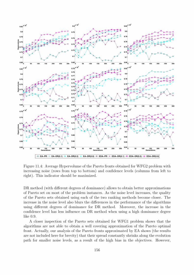
0 50 100 150 200 250 3009.68

9.7

9.72

9.74

9.76

9.78

9.8

9.82x 10

5

Hy

pe

rvo

lum

e

0 50 100 150 200 250 3009.68

9.7

9.72

9.74

9.76

9.78

9.8x 10

5

0 50 100 150 200 250 3009.68

9.7

9.72

9.74

9.76

9.78

9.8

9.82x 10

5

0 50 100 150 200 250 3009.68

9.7

9.72

9.74

9.76

9.78

9.8

9.82x 10

5

Hy

pe

rvo

lum

e

0 50 100 150 200 250 3009.69

9.7

9.71

9.72

9.73

9.74

9.75

9.76

9.77

9.78

9.79x 10

5

0 50 100 150 200 250 3009.68

9.7

9.72

9.74

9.76

9.78

9.8

9.82x 10

5

0 50 100 150 200 250 3009.66

9.68

9.7

9.72

9.74

9.76

9.78x 10

5

Hy

pe

rvo

lum

e

Generations0 50 100 150 200 250 300

9.64

9.66

9.68

9.7

9.72

9.74

9.76x 10

5

Generations

0 50 100 150 200 250 3009.64

9.66

9.68

9.7

9.72

9.74

9.76

9.78x 10

5

Generations

0.9 0.95 0.990

0.1

0.2

0.3

0.4

0.5

0.6

0.7

0.8

0.9

1

EA−PR EA−DR(0.1) EA−DR(0.5) EA−DR(0.9) EDA−PR EDA−DR(0.1) EDA−DR(0.5) EDA−DR(0.9)

Figure 11.4: Average Hypervolume of the Pareto fronts obtained for WFG2 problem withincreasing noise (rows from top to bottom) and confidence levels (columns from left toright). This indicator should be maximized.

DR method (with different degrees of dominance) allows to obtain better approximationsof Pareto set on most of the problem instances. As the noise level increases, the qualityof the Pareto sets obtained using each of the two ranking methods become closer. Theincrease in the noise level also blurs the differences in the performance of the algorithmsusing different degrees of dominance for DR method. Moreover, the increase in theconfidence level has less influence on DR method when using a high dominance degreelike 0.9.

A closer inspection of the Pareto sets obtained for WFG1 problem shows that thealgorithms are not able to obtain a well covering approximation of the Pareto optimalfront. Actually, our analysis of the Pareto fronts approximated by EA shows (the resultsare not included here for brevity) that their spread constantly shrinks along the evolutionpath for smaller noise levels, as a result of the high bias in the objectives. However,

156

0 50 100 150 200 250 3000.9

1

1.1

1.2

1.3

1.4

1.5

IGD

0 50 100 150 200 250 3000.8

0.9

1

1.1

1.2

1.3

1.4

1.5

0 50 100 150 200 250 3000.8

0.9

1

1.1

1.2

1.3

1.4

1.5

0 50 100 150 200 250 3000.9

1

1.1

1.2

1.3

1.4

1.5

IGD

0 50 100 150 200 250 3000.8

0.9

1

1.1

1.2

1.3

1.4

1.5

0 50 100 150 200 250 3000.9

0.95

1

1.05

1.1

1.15

1.2

1.25

1.3

1.35

1.4

0 50 100 150 200 250 3000.9

1

1.1

1.2

1.3

1.4

1.5

1.6

1.7

1.8

IGD

Generations

0 50 100 150 200 250 3001

1.1

1.2

1.3

1.4

1.5

1.6

1.7

1.8

Generations

0 50 100 150 200 250 3001

1.1

1.2

1.3

1.4

1.5

1.6

1.7

Generations

0.9 0.95 0.990

0.1

0.2

0.3

0.4

0.5

0.6

0.7

0.8

0.9

1

EA−PR EA−DR(0.1) EA−DR(0.5) EA−DR(0.9) EDA−PR EDA−DR(0.1) EDA−DR(0.5) EDA−DR(0.9)

Figure 11.5: Average IGD of the Pareto fronts obtained for WFG2 problem with increas-ing noise (rows from top to bottom) and confidence levels (columns from left to right).This indicator should be minimized.

the joint modeling adopted in EDA allows a better exploration of this problem’s searchspace, at least for lower noise levels, which is also reflected by the values obtained forhypervolume and IGD indicators.

The results obtained for WFG2 problem (Figures 11.4 and 11.5) also show that thePareto sets approximated with DR method are superior to those obtained using proba-bilistic ranking method. When a higher degree of dominance is used for the DR method,the performance of the algorithms with respect to the different quality indicators aremore sensitive to the increase in the length of the intervals, i.e. when increasing the levelof noise or confidence. In the last objective of this problem, the variables are consideredto be correlated and therefore, employing model learning to find out this relationshipshelps EDA to obtain better Pareto set approximations under different levels of noise andconfidence.

157

0 50 100 150 200 250 3009.73

9.74

9.75

9.76

9.77

9.78

9.79

9.8

9.81

9.82

9.83x 10

5

Hy

pe

rvo

lum

e

0 50 100 150 200 250 3009.66

9.68

9.7

9.72

9.74

9.76

9.78

9.8

9.82

9.84x 10

5

0 50 100 150 200 250 3009.66

9.68

9.7

9.72

9.74

9.76

9.78

9.8

9.82x 10

5

0 50 100 150 200 250 3009.7

9.72

9.74

9.76

9.78

9.8

9.82x 10

5

Hy

pe

rvo

lum

e

0 50 100 150 200 250 3009.66

9.68

9.7

9.72

9.74

9.76

9.78

9.8

9.82

9.84

9.86x 10

5

0 50 100 150 200 250 3009.64

9.66

9.68

9.7

9.72

9.74

9.76

9.78

9.8

9.82

9.84x 10

5

0 50 100 150 200 250 3009.7

9.72

9.74

9.76

9.78

9.8

9.82x 10

5

Hy

pe

rvo

lum

e

Generations0 50 100 150 200 250 300

9.66

9.68

9.7

9.72

9.74

9.76

9.78

9.8x 10

5

Generations

0 50 100 150 200 250 3009.66

9.68

9.7

9.72

9.74

9.76

9.78

9.8x 10

5

Generations

0.9 0.95 0.990

0.1

0.2

0.3

0.4

0.5

0.6

0.7

0.8

0.9

1

EA−PR EA−DR(0.1) EA−DR(0.5) EA−DR(0.9) EDA−PR EDA−DR(0.1) EDA−DR(0.5) EDA−DR(0.9)

Figure 11.6: Average Hypervolume of the Pareto fronts obtained for WFG3 problem withincreasing noise (rows from top to bottom) and confidence levels (columns from left toright). This indicator should be maximized.

Very similar results to those of the previous problem are obtained for WFG3 problem.The difference in the average performance of the algorithms using PR and DR methodsare clearer on this problem, and it can be seen that the solution ranking provided byPR method completely misguides the algorithms during evolution for approaching thePareto optimal set according to the quality indicators, even with small levels of noise andconfidence. The DR method using smaller dominance degrees results in relatively betteralgorithm performance on different levels of noise and confidence with respect to differentquality indicators.

The values of different indicators obtained for the Pareto sets approximated by EAand EDA are not consistent for this problem. According to hypervolume indicator, EAobtains relatively better results on WFG3 problem, whereas with respect to IGD indi-cator the results obtained by EDA outperform those of EA especially with larger noise

158

0 50 100 150 200 250 3000.95

1

1.05

1.1

1.15

1.2

1.25

IGD

0 50 100 150 200 250 3000.9

1

1.1

1.2

1.3

1.4

1.5

0 50 100 150 200 250 3000.9

1

1.1

1.2

1.3

1.4

1.5

1.6

0 50 100 150 200 250 3000.9

0.95

1

1.05

1.1

1.15

1.2

1.25

1.3

1.35

1.4

IGD

0 50 100 150 200 250 3000.9

1

1.1

1.2

1.3

1.4

1.5

1.6

1.7

1.8

0 50 100 150 200 250 3000.9

1

1.1

1.2

1.3

1.4

1.5

1.6

1.7

1.8

0 50 100 150 200 250 3001

1.05

1.1

1.15

1.2

1.25

1.3

1.35

IGD

Generations

0 50 100 150 200 250 3001

1.05

1.1

1.15

1.2

1.25

1.3

1.35

1.4

1.45

Generations

0 50 100 150 200 250 3001

1.05

1.1

1.15

1.2

1.25

1.3

1.35

1.4

Generations

0.9 0.95 0.990

0.1

0.2

0.3

0.4

0.5

0.6

0.7

0.8

0.9

1

EA−PR EA−DR(0.1) EA−DR(0.5) EA−DR(0.9) EDA−PR EDA−DR(0.1) EDA−DR(0.5) EDA−DR(0.9)

Figure 11.7: Average IGD of the Pareto fronts obtained for WFG3 problem with increas-ing noise (rows from top to bottom) and confidence levels (columns from left to right).This indicator should be minimized.

levels. WFG3 problem has a degenerated Pareto optimal front, and therefore a correctoptimization strategy would focus the search more around the lower-dimensional optimalfront during evolution. However, the hypervolume value of such a Pareto front will belower than a worse approximation which is more spread in the objective space. The IGDindicator on the other hand, computes the distance between points on the Pareto optimalfront and the approximated front, thus penalizing the more spread front in this case.

The objective functions of WFG7 problem are separable and unimodal, with bias inthe optimum values for some of the variables. The results obtained with DR method onthis problem outperform those of PR method with a relatively great margin, althoughthe increase in the noise level reduces the effectiveness of this ranking method, especiallywhen using it with EDA. Again, the Pareto fronts approximated with lower dominancedegrees for DR method are better. However, it can be seen that when the confidence

159

0 50 100 150 200 250 3009.62

9.64

9.66

9.68

9.7

9.72

9.74

9.76

9.78

9.8x 10

5

Hy

pe

rvo

lum

e

0 50 100 150 200 250 3009.64

9.66

9.68

9.7

9.72

9.74

9.76

9.78

9.8x 10

5

0 50 100 150 200 250 3009.64

9.66

9.68

9.7

9.72

9.74

9.76

9.78

9.8

9.82x 10

5

0 50 100 150 200 250 3009.64

9.66

9.68

9.7

9.72

9.74

9.76

9.78

9.8

9.82

9.84x 10

5

Hy

pe

rvo

lum

e

0 50 100 150 200 250 3009.6

9.65

9.7

9.75

9.8

9.85x 10

5

0 50 100 150 200 250 3009.62

9.64

9.66

9.68

9.7

9.72

9.74

9.76

9.78

9.8

9.82x 10

5

0 50 100 150 200 250 3009.6

9.62

9.64

9.66

9.68

9.7

9.72

9.74

9.76

9.78x 10

5

Hy

pe

rvo

lum

e

Generations0 50 100 150 200 250 300

9.65

9.7

9.75

9.8x 10

5

Generations

0 50 100 150 200 250 3009.64

9.66

9.68

9.7

9.72

9.74

9.76

9.78x 10

5

Generations

0.9 0.95 0.990

0.1

0.2

0.3

0.4

0.5

0.6

0.7

0.8

0.9

1

EA−PR EA−DR(0.1) EA−DR(0.5) EA−DR(0.9) EDA−PR EDA−DR(0.1) EDA−DR(0.5) EDA−DR(0.9)

Figure 11.8: Average Hypervolume of the Pareto fronts obtained for WFG7 problem withincreasing noise (rows from top to bottom) and confidence levels (columns from left toright). This indicator should be maximized.

level increases the performance of the algorithms using a high level of dominance degreeis less affected. In general, the search with EA results in relatively better Pareto frontapproximations comparing with the fronts obtained by EDA-based search according to thequality indicators values. Moreover, with the increase in the level of noise or confidence,which makes the problem harder, the results obtained by the two algorithmic frameworksbecome comparable.

The objective functions of WFG9 problem in contrast to those of the previous problemare non-separable and multi-modal, with multi-modality being deceptive towards localoptima for some of the objectives. As a result introducing noise to the objectives ofthis problem will make it very difficult to solve. The indicator values computed for theapproximated Pareto fronts show that the proposed DR method outperforms solution

160

0 50 100 150 200 250 3000.9

1

1.1

1.2

1.3

1.4

1.5

1.6

1.7

1.8

IGD

0 50 100 150 200 250 3000.9

1

1.1

1.2

1.3

1.4

1.5

1.6

1.7

1.8

0 50 100 150 200 250 3000.9

1

1.1

1.2

1.3

1.4

1.5

1.6

1.7

1.8

0 50 100 150 200 250 3000.9

1

1.1

1.2

1.3

1.4

1.5

1.6

IGD

0 50 100 150 200 250 3000.9

1

1.1

1.2

1.3

1.4

1.5

1.6

1.7

1.8

0 50 100 150 200 250 3000.8

1

1.2

1.4

1.6

1.8

2

0 50 100 150 200 250 3001

1.1

1.2

1.3

1.4

1.5

1.6

1.7

1.8

1.9

IGD

Generations

0 50 100 150 200 250 3001.05

1.1

1.15

1.2

1.25

1.3

1.35

1.4

1.45

1.5

1.55

Generations

0 50 100 150 200 250 3001

1.1

1.2

1.3

1.4

1.5

1.6

1.7

Generations

0.9 0.95 0.990

0.1

0.2

0.3

0.4

0.5

0.6

0.7

0.8

0.9

1

EA−PR EA−DR(0.1) EA−DR(0.5) EA−DR(0.9) EDA−PR EDA−DR(0.1) EDA−DR(0.5) EDA−DR(0.9)

Figure 11.9: Average IGD of the Pareto fronts obtained for WFG7 problem with increas-ing noise (rows from top to bottom) and confidence levels (columns from left to right).This indicator should be minimized.

ranking based on dominance probability, though with the increase in the noise level thedifference in the results obtained by the two methods gradually diminishes.

According to the results (Figures 11.10 and 11.11), lower dominance degrees likeα = 0.1 and α = 0.5 allow a better ranking of solutions in DR method. Moreover, onthe contrary to the previous problem, when the confidence level is increased DR methodwith higher dominance degree (α = 0.9) is also greatly affected. Comparing the EDAand EA based search, it is observed that the Pareto fronts approximated by EDA arecomparable or better to those obtained by EA, depending on the quality indicator. Thisbetter performance can be explained by the ability of the proposed EDA to capturethe relationships between variables of the problem, which is necessary for finding thesolutions.

161

0 50 100 150 200 250 3009.71

9.72

9.73

9.74

9.75

9.76

9.77

9.78

9.79

9.8

9.81x 10

5

Hy

pe

rvo

lum

e

0 50 100 150 200 250 3009.72

9.73

9.74

9.75

9.76

9.77

9.78

9.79

9.8

9.81

9.82x 10

5

0 50 100 150 200 250 3009.7

9.71

9.72

9.73

9.74

9.75

9.76

9.77

9.78

9.79

9.8x 10

5

0 50 100 150 200 250 3009.7

9.72

9.74

9.76

9.78

9.8

9.82x 10

5

Hy

pe

rvo

lum

e

0 50 100 150 200 250 3009.7

9.71

9.72

9.73

9.74

9.75

9.76

9.77

9.78

9.79

9.8x 10

5

0 50 100 150 200 250 3009.66

9.68

9.7

9.72

9.74

9.76

9.78

9.8x 10

5

0 50 100 150 200 250 3009.71

9.72

9.73

9.74

9.75

9.76

9.77

9.78

9.79x 10

5

Hy

pe

rvo

lum

e

Generations0 50 100 150 200 250 300

9.7

9.71

9.72

9.73

9.74

9.75

9.76

9.77

9.78

9.79x 10

5

Generations

0 50 100 150 200 250 3009.69

9.7

9.71

9.72

9.73

9.74

9.75

9.76

9.77

9.78

9.79x 10

5

Generations

0.9 0.95 0.990

0.1

0.2

0.3

0.4

0.5

0.6

0.7

0.8

0.9

1

EA−PR EA−DR(0.1) EA−DR(0.5) EA−DR(0.9) EDA−PR EDA−DR(0.1) EDA−DR(0.5) EDA−DR(0.9)

Figure 11.10: Average Hypervolume of the Pareto fronts obtained for WFG9 problemwith increasing noise (rows from top to bottom) and confidence levels (columns from leftto right). This indicator should be maximized.

11.5.4 Discussion

The values of the quality indicators for the Pareto sets obtained along the evolution path,show how the population of the different algorithm versions evolve. In general, based onthe change in the values of these indicators during evolution, we can see that the solutionranking provided by DR method guides the optimization in the correct direction throughthe search space of the tested MOPs, with some exceptions like WFG1 and WFG3 withhigh level of noise. On the contrary, when PR method is used for ranking the solutions,the algorithm is misguided in the search space of many of the tested problems (e.g. seeFigures 11.8 and 11.9).

When using DR method, the Pareto fronts approximated with smaller to mediumvalues of dominance degree α are better on most of the tested problems with different

162

0 50 100 150 200 250 3001

1.05

1.1

1.15

1.2

1.25

1.3

1.35

IGD

0 50 100 150 200 250 3000.95

1

1.05

1.1

1.15

1.2

1.25

1.3

1.35

1.4

0 50 100 150 200 250 3001

1.05

1.1

1.15

1.2

1.25

1.3

1.35

1.4

0 50 100 150 200 250 3000.9

0.95

1

1.05

1.1

1.15

1.2

1.25

1.3

1.35

1.4

IGD

0 50 100 150 200 250 3000.9

1

1.1

1.2

1.3

1.4

1.5

0 50 100 150 200 250 3000.9

1

1.1

1.2

1.3

1.4

1.5

0 50 100 150 200 250 3001

1.05

1.1

1.15

1.2

1.25

1.3

1.35

IGD

Generations

0 50 100 150 200 250 3001

1.05

1.1

1.15

1.2

1.25

1.3

1.35

1.4

Generations

0 50 100 150 200 250 3001

1.05

1.1

1.15

1.2

1.25

1.3

1.35

1.4

1.45

Generations

0.9 0.95 0.990

0.1

0.2

0.3

0.4

0.5

0.6

0.7

0.8

0.9

1

EA−PR EA−DR(0.1) EA−DR(0.5) EA−DR(0.9) EDA−PR EDA−DR(0.1) EDA−DR(0.5) EDA−DR(0.9)

Figure 11.11: Average IGD of the Pareto fronts obtained for WFG9 problem with in-creasing noise (rows from top to bottom) and confidence levels (columns from left toright). This indicator should be minimized.

levels of noise and confidence. On the one hand, smaller values of α allow higher degrees ofoverlapping between intervals, meaning that the solutions can dominate each other easier.With small values of α, according to Corollary 11.2 the ratio of dominated solutionsincreases and therefore more solutions become comparable, resulting in a finer ordering ofthe solutions by the employed α-degree non-dominated sorting algorithm. This increase inthe number of comparable solutions seems to compensate for the lack of strict decisions onthe quality of the solutions. On the other hand, strict decisions about solution dominanceallow only very good solutions to enter the α-degree non-dominated set, while causingmany solutions to become incomparable. Based on the experimental results, with acombination of the previous two effects which is achieved when using medium values ofdominance degree (e.g. α = 0.5), better Pareto set can be approximated on many of thetested MOPs and for different levels of noise and confidence.

163

Similarly, as the confidence level of the intervals (i.e. the values of the objectivefunctions) decreases, more and more solutions become dominated (Corollary 11.1), andthus the solutions will be ordered in a larger number of α-degree non-dominated setsduring the first step of Algorithm 11.1, essentially leading to better solution ranking.Therefore, when DR method is used in the optimization the Pareto sets approximatedfor lower confidence levels are usually better, according to the quality indicator values.Taking more strict decisions by using high dominance degrees (e.g. α = 0.9) when theconfidence level increases, reduces the number of α-degree non-dominated sets found inthe first step of Algorithm 11.1, and thus the ordering of the solutions will depend more ontheir crowding distance computed in the second step of α-degree non-dominated sortingalgorithm. For some of the tested problems (e.g. WFG1 and WFG7), such an orderingwith high α values seems to be less affected as the confidence level increases.

11.6 Conclusions

In real-world multi-objective optimization, the value of objective functions may involvenoise and thus do not correctly represent the quality of solutions. Population-basedEAs, which are one of the most successful methods in solving MOPs, have inherentabilities to deal with small levels of noise in objective values. However, with larger noiselevels, especially when there are several conflicting objectives to be optimized, specificconsiderations are needed to perform successful optimization.

We considered noisy objective values given as intervals and proposed α-degree Paretodominance to deal with this type of values for the objective functions. This relationallowed to determine the dominance between solutions even when there is a specific degreeof overlapping between some of the interval values, which is controlled by parameter α.The similarity between this dominance relation and the conventional Pareto dominanceallowed related terminology, like Pareto optimal set, to be easily defined. Assumingconfidence intervals with a specific confidence level as the values of the noisy objectivefunctions, we studied some of the properties of α-degree Pareto dominance. It was shownthat the α-degree dominance relations defined between solutions are unaffected when theconfidence level γ or dominance degree α are reduced, and that such a reduction decreasesthe size of Pareto optimal set.

Based on this relation, α-degree Pareto non-dominated sorting algorithm, an adapta-tion of the well-known non-dominated sorting algorithm in noisy domains with intervalvalues, was proposed and integrated into MBN-EDA to find the solutions of noisy MOPs.The algorithm was tested on a set of MOPs where noisy objective values are given asintervals, and its solution ranking and search space exploration were respectively com-pared with a reference ranking method based on dominance probability and standard EAoperators for continuous optimization.

The analysis of the approximated Pareto sets with two different quality indicatorsbased on the corresponding noiseless Pareto fronts showed that the proposed solutionranking method based on α-degree Pareto dominance relation allows the algorithms toachieve considerably better results comparing with the well-known probabilistic rankingmethod on the tested problems and for increasing levels of noise and confidence. Wediscussed how the change in the dominance degree and confidence level changes compa-

164

rability of the solutions using α-degree Pareto dominance relation. Moreover, dependingon the specific properties of the MOPs, the quality indicator values showed that the jointprobabilistic modeling of variables and objectives allowed MBN-EDA to find Pareto setapproximations for some of the tested noisy problems that are superior to those approx-imated by the standard multi-objective EA in different levels of noise.

165

166

Chapter 12

An Interval-Based Multi-ObjectiveApproach to Feature SubsetSelection Using Joint ProbabilisticModeling

12.1 Introduction

In its simplest form, a (supervised) classification task in data mining is to use a set oflabeled data points to induce a classifier model, which can then be used to predict thelabel of new data points. The input data points are characterized by a number of featurevalues and a label, which identifies the class-value of each point. By features, we refer tothe attributes or columns of a dataset and we use class to refer to the column containingthe label or class-value of the data points. The classifier induced from the input data isused to find the class-value of an unlabeled data point, given its feature values.

A well-known problem related to classification is to find the subset of features thatshould be used for determining the class-values [Liu and Motoda, 1998], often referred toas feature subset selection (FSS). Selecting an appropriate subset of features can reducethe overall computational complexity and improve the classification accuracy. Therefore,usually an additional step is carried out before/whilst learning the classifier model froma training dataset to search for an appropriate subset of features, especially in high-dimensional problems with a large number of features. Moreover, the space of all possiblefeature subsets is huge, making it impossible to use exhaustive search methods to findthe optimal feature subset(s) according to some optimization criteria. Therefore, a verygood candidate for searching this space is to use stochastic heuristics. Especially, EAshave been used for FSS, as we saw in Section 3.6 for the case of Bayesian classifiers. Oneof the approaches to FSS which has gained a lot of attention in the past few years ismulti-objective optimization. An important motivation for this approach is the intrinsicconflict between problem goals (e.g. maximize accuracy and minimize model complexity)which cannot be easily aggregated to a single objective.

Usually, the objectives considered for FSS cannot be computed directly from eachsubset of features. Instead, the objectives are estimated using a set of data pointswith/without a simulation process. Therefore, there is an inherent uncertainty in the

167

objective values obtained for feature subsets, which varies depending on the method anddata points used for estimation. The optimization algorithm employed for FSS shouldtake into account the noise in objective values during search. The noise handling tech-niques explained in Chapter 11 are especially useful for this purpose.

In this chapter, we adapt MBN-EDA for solving the FSS problem formulated as anMOP with six objective functions. These functions, whose values describe the perfor-mance of a classifier, are the area under the ROC curve, sensitivity, specificity, precision,F1 measure and Brier score. Following the discussion in the previous chapter, we considerinterval values for each of these objectives to deal with the noise in their values. Theseintervals are obtained from estimating the objectives in different conditions (e.g. withdifferent sets of data points). We propose a solution ranking method based on α-degreePareto dominance relation to select a subset of solutions in each generation.

Since the feature subsets are encoded as binary strings, the joint probabilistic modelin MBN-EDA should be estimated in a mixed discrete-continuous domain. We proposea two-step approach for joint modeling of variables and objectives in MBN-EDA. In thefirst step, `1-regularization is used to identify the set of more relevant variables to eachobjective. In the second step, an MBN is estimated as the joint model of variablesand objectives, starting from the initial structure approximated in the first step. Thismethod simplifies the estimation of joint model by removing irrelevant variables. More-over, thanks to the interactions encoded in the joint model, we can study the relationshipsbetween the objectives considered for this problem, something which is less studied sofar in FSS.

12.2 EMO Algorithms in FSS

FSS can be formally expressed as selecting the best subset of features for a learner model,given the set of all candidate features [Inza et al., 2000]. Therefore, the objective of FSSis to reduce the number of features used to characterize the dataset while improving theperformance of the learner model on that dataset. According to Blum and Langley [1997],an FSS method should address the following issues:

1. Initial point: the starting point(s) of the search process. It can be an empty subset(i.e. no features selected), a full subset or a randomly generated subset.

2. Search strategy: the algorithm used to explore the space of possible feature subsets.This space is exponential in the number of features (2n–where n is the number offeatures), and thus FSS is considered to be a difficult combinatorial problem withan intractable computational complexity [Davies and Russell, 1994; Liu and Yu,2005].

3. Feature subset evaluation: measuring the quality of different feature subsets, so thathigh quality subsets can be preferred over others. Generally, two major approachesto feature subset evaluation exist. The wrapper approach uses the performance ofa learner model, trained with the features in a subset, as the evaluation criteria ofthat subset. In the filter approach, instead of the learner model performance, data-driven measures (e.g. correlation, mutual information, etc.) are used to evaluatethe subset of features.

168

4. Search stopping criteria: determine how the search method will be terminated.For example insignificant change in the quality of feature subsets, or reaching amaximum number of feature subset evaluations.

Apart from the above mentioned filter and wrapper approaches, there is another lessfrequently approach called embedded FSS, where feature selection takes place duringthe training of the learner model. `1-regularized model learning is an example of thesemethods.

A search algorithm for FSS deals with three different spaces. First, the space of allpossible feature subsets which defines the search space. This is the space that the searchalgorithm explores. Second, the samples in the dataset represent points in the data space.For each solution in the search space, a different projection of the data space, obtainedaccording to the features included in that solution, is used to evaluate the solution (e.g.by training and testing a learner model). Third, the result of evaluating each solution isa point in the objective space. Viewed in this way, feature subset evaluation is a functionthat maps each solution in the search space through data space to a point in the objectivespace.

Both wrapper and filter approaches have been used for evaluating feature subsetswhen using EMO algorithms for FSS. To evaluate a solution (i.e. feature subset) within awrapper approach, first a learner model is trained using a training dataset and only takingthe features included in that solution. Then this model is tested on a separate validationor test dataset to assess its performance. To increase the accuracy of the assessment,usually this process is repeated several times. Techniques like bootstrapping, k-foldcross-validation or leave-one-out (a special version of the latter) are used for partitioningthe dataset and repeated evaluation of a learner model.

This way of evaluating solutions has a high computational complexity. However, fromthe perspective of learner model performance, the solutions found with this approachare often superior to those found with filter-based methods. Therefore, most of theEMO algorithms for FSS are based on a wrapper approach, which uses the k-fold cross-validation of a usually simple learner model with short training time. Some of the methodshave also used distributed evaluation to speed up solution evaluation [Oliveira et al., 2006],or approximation techniques to prevent retraining the classifier for each single solution[Emmanouilidis et al., 2001; Oliveira et al., 2002].

Techniques like bootstrapping and k-fold cross-validation can obtain a good estima-tion of the quality of each solution. However, more accurate estimation of quality can beobtained by testing the final solutions found by the search algorithm on an independentdataset which is not used during the search algorithm. Moreover, to have a statistical es-timation of a search algorithm performance in FSS, that algorithm should be run severaltimes. Thus, to combine these two requirements for quality and performance assessment,several bi-partitions of the given dataset are considered. For each bi-partition, two indi-vidual runs of the search algorithm are performed. In the first run, one of the partitions isused to evaluate the solutions during the search process (e.g. by a k-fold cross-validationmethod) and after the search, the other partition is used to test the final solutions. Inthe second run the role of the partitions is exchanged.

In the following two sections we briefly review some of the works in the literature thatuse EMO algorithms for FSS. These works are summarized in Table 12.1. The intuitivemethod of representing a feature subset, adopted by all of the algorithms reviewed here,

169

is to use a binary encoding, i.e. a bit string of length equal to the number of features,where a zero value means the exclusion of the corresponding feature from the subset anda value of one means its inclusion. Thus, there is a one to one correspondence betweenthe features of the dataset and the variables in the solutions to the FSS problem.

12.2.1 FSS in Classification

Emmanouilidis et al. [2000] proposed a commonality-based crossover in the context ofniched Pareto GA (NPGA) [Horn et al., 1994], where common alleles of the parent so-lutions are directly copied to the offspring solutions, and the other genes are inheritedbased on a probability computed from the number of common genes. They used the clas-sification accuracy of artificial neural networks (ANN) together with the size of featuresubset as the objectives of optimization. They also applied their method to the rotat-ing machinery fault diagnosis problem with respectively two (approximated root meansquared error of ANN and feature subset size) [Emmanouilidis et al., 2001] and threeobjectives (sensitivity and specificity of a nearest neighbor (NN) classifier and the size offeature subset) [Emmanouilidis, 2001].

Oliveira et al. [2002] used the first version of non-dominated sorting GA (NSGA)[Srinivas and Deb, 1994], which is based on fitness sharing, to select a good subset offeatures for handwritten digit recognition problem. The classification accuracy of anANN classifier and the size of feature subsets were used as optimization objectives. Theyalso used EMO algorithms to search for the best ensemble of the classifiers found in thePareto set after FSS search [Oliveira et al., 2006].

Some other works have used NSGA-II to search for good feature subsets in FSSproblems. Shi et al. [2004] tried to find the best feature subsets for an ensemble of supportvector machines (SVMs) in the protein fold recognition problem. Three objectives wereused for optimization: 1) cross-validation classification accuracy, 2) test classificationaccuracy, and 3) feature subset size. Hamdani et al. [2007] studied the performanceof NSGA-II for FSS on several datasets of varying sizes. They used the classificationaccuracy of an NN classifier and feature subset size as optimization objectives. Ekbalet al. [2010] searched for relevant features of the named entity recognition problem inthe field of natural language processing with a wrapper method which uses maximumentropy-based classifiers. Recall and precision of the classifiers were used as objectivesduring the search process, and F-measure was used to select one of the feature subsetsfrom the final Pareto set. Instead of considering all feature subset sizes together, Huanget al. [2010] performed separate optimizations for each of the feature subset sizes in theproblem of predicting customer churn in telecommunications. Classification accuracy,true positive rate and true negative rate of a decision tree (DT) classifier were used asobjectives in each of the optimization runs.

In a different context, Rodrıguez and Lozano [2008] used NSGA-II to perform a multi-objective search for the best structure of an MBN, which involves selecting the subset offeatures relevant to each class variable. They used the classification accuracy of each of theclasses as the optimization objectives. Radtke et al. [2009] proposed a three phase multi-objective optimization scheme for: 1) feature extraction, 2) single classifier or ensemblecomponents selection, and 3) FSS to improve the performance of the selected classifier orensemble. They compared the performance of NSGA-II and a multi-objective memetic

170

Table 12.1: Summary of the methods for FSS using EMO algorithms.

Ap

proa

chO

ptim

izerL

earn

erM

od

el#

Ob

jectives

Classification

[Em

man

ou

ilidis

etal.,

2000

]W

rapp

erN

PG

AA

NN

2

[Em

man

ou

ilidis

etal.,

2001

]W

rapp

erN

PG

AA

NN

2

[Em

man

ou

ilidis,

2001

]W

rapp

erN

PG

A1-N

N3

[Oliveira

etal.,

2002

]W

rapp

erN

SG

AA

NN

2

[Oliveira

etal.,

2006

]W

rapp

erN

SG

AA

NN

2

[Sh

iet

al.,2004]

Wrap

per

NS

GA

-IIE

nsem

ble

ofS

VM

s3

[Ham

dan

iet

al.,20

07]

Wrap

per

NS

GA

-II1-N

N2

[Rod

rıgu

ezan

dL

ozan

o,

2008

]W

rapp

erN

SG

A-II

MB

N2

[Ekb

al

etal.,

2010]

Wrap

per

NS

GA

-IIM

ax

entrop

y-b

asedclassifi

er2

[Hu

an

get

al.,

2010]

Wrap

per

NS

GA

-IID

T3

[Rad

tkeet

al.,

2009

]W

rapp

erN

SG

A-II,

Mem

eticE

MO

AN

N,

Pro

jectiond

istance-b

ased

classifier

2

[Vato

lkin

etal.,

2012

]W

rapp

erIn

dica

tor-b

ased

EM

OD

T,

Ran

dom

forest,N

B,

SV

M2

[Zhu

etal.,

2009]

Hyb

ridM

emetic

EM

OD

T3,

4

[Sp

olaoret

al.,

2011]

Filter

NS

GA

-II—

2

Clustering

[Kim

etal.,

2002

]W

rapp

erE

LS

AK

-mea

ns,

EM

3,4

[Morita

etal.,

2003]

Wrap

per

NS

GA

K-m

ean

s2

[Zh

an

get

al.,20

06]

Wrap

per

Imm

un

olo

gy-b

ased

EM

OF

uzzy

c-mean

s3

[Han

dl

an

dK

now

les,20

06]

Wrap

per,

Filter

PE

SA

-IIK

-mea

ns

2

[Zah

arieet

al.,2007]

Filter

NS

GA

-II—

4

171

algorithm on the handwritten digit recognition problem, with respect to classificationaccuracy and feature subset size as objectives.

Zhu et al. [2009] used a hybrid wrapper-filter approach by combining wrapper-basedNSGA-II and filter-based local search in a memetic algorithm. The accuracies of eachof the class-values in a one-versus-all classification scheme, obtained from DT classifiers,were used as optimization objectives in NSGA-II, whereas the criterion for local searchwas based on the feature-class relevance. Spolaor et al. [2011] proposed several filter-based bi-objective optimizations using NSGA-II for FSS, each time pairing interclassdistance measure with one of the following criteria: ratio of inconsistent pairs of samplesin the dataset, feature-class correlation, Laplacian score of the samples in the dataset,and features entropy.

Very recently, Vatolkin et al. [2012] employed a hypervolume indicator-based EMOalgorithm to search for good feature subsets in the high-dimensional problem of musicalinstruments recognition in a polyphonic audio mixture. They used the relative featuresubset size and mean squared error of classification as optimization objectives. DTs,random forests, NBs and SVMs were used as alternative classifiers to compute the secondobjective.

12.2.2 FSS in Clustering

In the context of unsupervised learning or clustering, the solution encoding may be ex-tended to also include the number of clusters. Thus, the algorithm will be simultaneouslysearching the space of possible feature subsets and the space of possible numbers of clus-ter. The learner model in this context is a clustering algorithm which assigns the samplesin the dataset to a number of clusters. The objectives here are usually based on increasingthe closeness of the samples in the same cluster (cluster compactness), while increasingthe separation between different clusters.

Kim et al. [2002] proposed an evolutionary local search algorithm (ELSA) to selectthe proper subset of features for clustering. They proposed four objectives when usingthe K-means algorithm and three objectives when using the EM algorithm for clustering.Morita et al. [2003] used NSGA with two objectives for FSS when clustering handwrittenmonth names with the K-means algorithm. Handl and Knowles [2006] proposed a generalframework for bi-objective FSS in clustering problems which encompasses both filter andwrapper approaches. Their framework is based on the second version of Pareto envelope-based selection algorithm (PESA-II) [Corne et al., 2001] and uses the K-means algorithmfor clustering when the objectives are evaluated with the wrapper approach.

Instead of representing the feature subsets with bit strings, Zhang et al. [2006] encodefeature saliencies in real-valued strings and select only those features with a saliencyvalue above a given threshold. They employed an immunology-based EA to solve athree-objective optimization problem by using a fuzzy c-means algorithm for clustering.Zaharie et al. [2007] used NSGA-II, with four different objectives in a filter approach, tofind the best ranking of the features, a problem closely related to FSS.

172

Figure 12.1: The overview of the proposed EDA for FSS in classification.

12.3 Multi-Objective FSS with Joint Modeling of Vari-

ables and Objectives

In the following sections we explain the essential steps of the algorithm proposed for FSS.The algorithm, which is an adaptation of MBN-EDA for FSS, employs a solution rankingmethod based on α-degree Pareto dominance for dealing with the noise in the objectivevalues when selecting a subset of solutions. A special method is proposed for learning ajoint probabilistic model of variables and objectives for this problem. Figure 12.1 showsthe overall outline of the proposed algorithm.

12.3.1 Solution Ranking

In the last chapter, we saw that one of the ways to increase the confidence in the objec-tive values returned for a noisy MOP is the reevaluation of objective functions on eachsolution. However, in some of the MOPs, solution evaluation inherently involves multi-ple reevaluations. In the case of FSS problem, when the feature subsets are evaluatedusing k-fold cross-validation or bootstrapping, a set of values are obtained for each of theobjectives. These values are then averaged to obtain a more accurate estimation of thequality of each feature subset.

Instead of estimating singular values as the value of each objective using these reeval-uations, an alternative approach, which has been less studied so far, is to use all of the

173

reevaluation values, representing the quality of each solution under different conditions,and assume that each objective function returns interval values. We saw that in this waythe algorithm can take into account the noise in objective values when selecting a subsetof solutions.

Having interval values for the objectives, the PR method based on probabilistic dom-inance can be used for ordering the solutions, as was explained in the last chapter. How-ever, the computational complexity of calculating the probabilities when using this rank-ing method is one of its major drawbacks. Here, we propose a method for orderingthe solutions based on α-degree Pareto dominance, called degree ranking (DR). In thismethod, first the solutions in the population are sorted into a number of α-degree Paretosets, and then the rank of each solution xi within the population is computed as

rankDR(xi) = θND · ri +1

N

N∑k=1

m∑j=1

degj(xk,xi) + θB ·m∑j=1

I(⌊fj(xi)

⌋, f ∗j), (12.1)

where ri is the rank of the α-degree Pareto set containing solution xi (starting from 1for the best Pareto set). I(a, b) is an indicator function returning one if a is equal to band zero otherwise, and f ∗j is the best value reached so far in the jth objective. Here, we

are assuming a minimization problem and therefore⌊fj(xi)

⌋shows the best point of the

interval value obtained for fj(xi). θND and θB are the scaling coefficients determiningthe importance of respectively α-degree Pareto ranks and best-found boundary values inranking the solutions.

The ranking method in Equation (12.1) combines the measures of solution conver-gence and dispersion with α-degree Pareto ranks. This measures are very similar to thegain-based and distance to best-based ranking methods [Garza-Fabre et al., 2009, 2010a]that where individually used for multi-objective optimization in Chapter 10. The secondand third terms of Equation (12.1) can be computed while sorting the solutions intoα-degree Pareto non-dominated sets (which has a complexity of order O(N2m)). Thus,their computation does not impose additional computational overhead like when com-puting crowding distances in the adapted non-dominated sorting algorithm used in theprevious chapter. Since solution ranking is one of the most time consuming steps in EMOalgorithms, this reduction in computational time is highly favorable.

12.3.2 Joint Model Learning

As it was explained in Section 12.2, FSS is a combinatorial problem with a discretesearch domain where candidate solutions are represented with bit strings. However,the objectives considered for this problem are usually continuous-valued functions or, asassumed in Section 12.3.1, functions with interval values. Although, as it was reviewedin Chapter 1, there are some approaches for learning probabilistic models in domainswith mixed continuous-discrete variables, but their application to the joint modeling ofvariables and objectives in our algorithm will be computationally very demanding, andthus can not scale well due to its complexity. The method we propose here for learninga joint model of variables and objectives consists of two major steps. Figure 12.1 showsthe outline of this approach.

174

Inputs:Selected solutions DXTheir objective values DF

� First part

1 DEF ← Estimate expected values of objectives from DF2 for all fj ∈ F do

3 MR[X, fj ]← Estimate an RRM from(DX ,DEfj

)4 end for5 XS ← Combine variables selected in MR[X, fj ],∀fj ∈ F6 XS ←X \XS

7 SI [XS ,F ]← Initialize to empty structure8 for all fj ∈ F do9 MR[XS , fj ]← Remove variables in XS from MR[X, fj ]

10 SI [XS ,F ]← SI [XS ,F ]+ Structure of MR[XS , fj ]11 end for

� Second part

12 DDF ← Discretize objective values in DEF13 M1[XS ,F ]← Estimate an MBN from

(DXS

,DDF)

starting from the structure SI [XS ,F ]14 for all Xi ∈ XS do15 M2[Xi]← Estimate univariate probability distribution from DXi16 end for

Output:(M1[XS ,F ], {M2[Xi] | Xi ∈ XS}

)Algorithm 12.1: Outline of the joint model estimation method.

Variable Selection with Regularized Regression

In the first part of the joint modeling algorithm, we adopt a method similar to the firstapproach of regularized model learning in Section 5.2, based on regularized regression,for finding the most related subset of variables to each objective. Formally, let the set{(x1,f(x1)

), . . . ,

(xN ,f(xN)

)}denote a joint dataset of variable-objective values, with

objective values given as confidence intervals. Then, we learn an `1 regularized regressionmodel (RRM) (Section 4.2) for each objective fj given the variables:

arg minβj

( N∑i=1

(E(fj(xi)

)−(βj<0> +

n∑k=1

βj<k>xi<k>))2

+ λn∑k=1

|βj<k>|). (12.2)

In this equation, the estimated expected values of each objective are used to estimatethe RRM parameters, which as explained in Section 11.4.2 can be a good representativeof the corresponding interval values. The n + 1-dimensional vector βj is the parameterestimated for the RRM of the jth objective. AIC [Akaike, 1974] is used as the scoringmetric to select between different parameter vectors for each RRM. Because of the variableselection property of `1 regularization, each of the estimated RRMs shows the subset ofvariables which is more relevant to the corresponding objective. Bearing in mind that injoint modeling of variables and objective with MBN, the bridge subgraph also encodes

175

a kind of variable selection for each objective, the estimated RRMs can be used as anapproximation of the initial structure of this subgraph.

At the end of this part of joint modeling, the subset of variables selected for each of theobjectives in the RRMs are combined to obtain a common subset of most relevant featuresto all objectives. In Section 4.3 we saw that strategies like the union or the intersection ofthe variable subsets can be used for combining these subsets [Meinshausen and Buhlmann,2006]. Here, we adopt an intermediate approach by selecting those variables that haveappeared in at least half of the RRMs. As a result, the set of variables are divided intotwo groups: those selected in the combined model, XS, and the rest, XS = X \XS.

MBN Estimation

In the second part, an MBN is estimated, modeling the objectives and variables in XS.For this purpose, using an equal frequency discretization method, the objective valuesare discretized into three nominal values: good, average and bad. Before starting thegreedy local search for estimating MBN, its structure, or more specifically its bridgesubgraph, is initialized with the structure of the combined model obtained in the first part.Our experiments have shown that this initialization can highly reduce the search effortneeded to find a good MBN structure with greedy local search, as they are usually goodapproximations of the interactions encoded in the bridge subgraph. Since the variablesand objectives are discrete, the parameters encoded in all MBN nodes are conditionalprobability tables which are used to evaluate different MBN structures with the BICscoring metric, as formulated in Equation (1.8).

The variables in XS, which are considered less important to the objectives, can beignored in the modeling process, only copying their values when generating new solutions.However, to allow the possibility of future participation of these variables in joint modeling(in the next generations), we estimate a univariate marginal probability distribution foreach variable in XS (similar to UMDA [Muhlenbein and Paaß, 1996]) to explore thesubspace of these variables with a low-complexity modeling.

At the end, the adaptation of joint probability distribution of variables and objec-tives, presented in Equation (10.2), which is now encoded in both MBN and individualunivariate probability distributions, is given by

P(x1, . . . , xn, q1, . . . , qm

)=

∏Xi∈XS

P (xi|pai) ·∏

Xk∈XS

P (xk) ·m∏j=1

P (qj|pa′j). (12.3)

All of the notations in this equation have the same meaning as in Equation (10.2). Forexample, q = (q1, . . . , qm) denotes a possible discrete value-setting for the objective vari-ables Q = (Q1, . . . , Qm).

The probability distribution of Equation (12.3) is used in the sampling step of MBN-EDA to generate new candidate solutions. For the variables included in the MBN (XS),the second sampling approach described in Section 9.3.2 is used to generate new valuesaccording to the objective values encoded in the joint model. For the rest of the vari-ables (XS), new values are sampled from their estimated univariate marginal probabilitydistributions.

176

12.4 Problem Formulation

This section describes how FSS is formulated as an MOP to be solved by the proposedadaptation of MBN-EDA. We use a wrapper approach to evaluate feature subsets withtwo different Bayesian classifiers, namely the NB and TAN classifiers. It should be notedthat these two classifiers define two different optimization problems on each dataset sincethe best feature subset obtained for one type of classifier might not necessarily be thebest feature subset for another type of classifier.

The NB classifier training consists only of finding the prior probability of class-valuesand the conditional probabilities of each feature values. Despite its simple structure,NB classifier is shown to have very good classification performance in many real-worldproblems. The TAN classifier training algorithm involves finding the maximum weightedspanning tree over the features, based on their conditional mutual information given theclass. It is proven that this algorithm learns the maximum log-likelihood TAN classifierfor a given dataset [Friedman et al., 1997].

These two classifiers choose the class-value with the highest posterior probability asthe predicted label of a given value-setting x of features. In a binary classification problem(i.e. when there are only two different class-values) the predicted class-values for a setof data points can be compared against their true class-values to assess the accuracy ofthe classification. Assuming that the class-values assigned to the data points are eitherpositive or negative, the number of correct (true) and wrong (false) classifications areusually organized as follows in a data structure called confusion matrix:

True Label

Positive Negative

Pre

dic

ted

Lab

el

Posi

tive True False

Positive Positive

(TP) (FP)

Neg

ativ

e False True

Negative Negative

(FN) (TN)

In this matrix, TP and TN show the number of correct classifications in each of the classes,whereas FP and FN show the number of data points which where wrongly classified.

We use six different performance measures, based on the classification accuracy givenin the confusion matrix and the encoded class-value probabilities, to evaluate the clas-sifiers on a test set. These measures are: sensitivity, specificity, precision, area underreceiver operating characteristics curve (AUC), F1 and Brier score, and are computed as

177

follows:

fAUC =G1 + 1

2,

fsens =TP

TP + FN,

fspec =TN

TN + FP,

fprec =TP

TP + FP,

fF1 =2TP

2TP + FN + FP,

fBrier =1

N

N∑i=1

C∑k=1

(P (ck | xi)− δ(ck,xi)

)2, (12.4)

where G1 is the Gini coefficient estimated by approximating the area under the Lorenzcurve [Gastwirth, 1972]. N is the total number of samples, i.e. N = TP+TN+FP+FN .C is the number of possible class-values: {c1, . . . , cC}, and function δ(ck,xi) returns oneif the true class-value of instance xi is ck and zero otherwise. These measures definethe objective functions of optimization. The first five objectives should be maximizedand have a range of values in [0, 1], whereas the last objective should be minimized andrepresents the calibration error in classification.

Following the common practice in FSS literature, we use binary encoding to representfeature subsets with bit strings of length equal to the number all features. Each featuresubset is evaluated using k-fold cross-validation of a classifier on a given dataset, projectedover the features in the subset. Thus, we will obtain k values for each of the classifierperformance measures (objectives). These values are then used to compute a confidenceinterval with a confidence level γ ∈ [0, 1] for each of the performance measures.

12.5 Experiments

We have used three datasets with an increasing number of features to study the perfor-mance of our proposal for FSS. These datasets, which are all retrieved from UCI onlinemachine learning repository1, are Wisconsin diagnostic breast cancer (WDBC), ozonelevel detection (Ozone) and Hill-Valley, with details presented in Table 12.2. To handlethe missing values in the Ozone dataset, we discard samples with missing class-value, orif half of the features are missing. Otherwise, the missing values are replaced with themean value of that feature.

The Pareto optimal set of a FSS problem is not known beforehand. Therefore,the three quality indicators of hypervolume, maximum spread [Zitzler et al., 2000] andSchott’s spacing [Schott, 1995] are used to respectively examine the convergence, diver-sity and distribution of the final Pareto fronts approximated by the algorithm. Theseindicators are computed using the expected values of the objectives. As it was defined

1http://archive.ics.uci.edu/ml/datasets.html

178

Table 12.2: Datasets considered for the experiments

Name # samples # features # class-values Missing values

WDBC 569 30 2 No

Ozone 2536 72 2 Yes

Hill-Valley 2424 100 2 No

in Equation (10.11), hypervolume indicator computes the total hyper-volume of the ob-jective space that is dominated by the solutions in the approximated Pareto front, andlarger values of this indicator show better approximations.

Maximum spread indicator gives an estimation of the Pareto front diversity by takinginto account the minimum and maximum values achieved for each objective. Given aPareto set approximation A, this indicator is computed as

MS(A) =

√√√√ m∑j=1

maxx,y∈A

d(fj(x), fj(y)

). (12.5)

Larger values of this indicator show a more diverse front and are desired. Schott’s spacingindicator is a measure of how evenly the approximated Pareto front is distributed. It isdefined as the standard deviation of distances between each solution and its nearestneighbor in the objective space. Specifically, given a Pareto set approximation A, thedistance contribution of a solution y ∈ A to the value of this indicator is computed as

minx∈A,x6=y

d(f(x),f(y)

),

where d(·, ·) can be any distance function like city-block or Euclidean distance. Lowervalues of Schott’s spacing indicator are favored.

12.5.1 Experimental Design

To evaluate the performance of the proposed algorithm, 5 random bi-partitions of eachdataset are generated (elsewhere this method is called 5 × 2 cross-validation), resultingin 10 independent runs. For each run, the number of cross-validation folds is set tok = 5 and a confidence level of γ = 0.95 is used to compute the intervals for the perfor-mance measures (objectives). The evaluation of the final Pareto set of each run on theindependent test set is used to compute the final Pareto front approximated in that run.

The initial population of MBN-EDA is generated randomly with a uniform distribu-tion. The full set of features and the empty subset are also added to the initial populationto provide both of the possible values for all of the variables in the initial population.The population size is set to N = 2, 000 to provide adequate statistics for the estima-tions of MBN parameters. Such a population size is also suggested in other works usingBN-based EDAs for FSS [Inza et al., 2000]. When estimating the MBN structure, themaximum number of parents for each node is set to max{m, dlog3(τN)e}, allowing thepossibility for the variable nodes to have all objectives as their parents, while preventingvery complex structures. In our experiments, the MBN learning algorithm virtually never

179

needed to surpass this maximum (in less than 0.15% of model estimations an operationwas canceled because of reaching this maximum), which shows its negligible influence onMBN estimation. To compensate for the large population size requirement of MBN-EDA,we set the maximum number of generations to 50.

12.5.2 MBN-EDA with Different Solution Ranking Methods

In the first set of experiments, the feature subsets found by MBN-EDA when using PR andDR methods for solution ranking are compared and analyzed. PR is computed based onthe simplifying assumption of Equation (11.8) and the approximation of Equation (11.9).Similar to the previous chapter, three different degrees of dominance are studied for the α-degree Pareto dominance relation in DR method, i.e. α ∈ {0.1, 0.5, 0.9}. When choosingthe values of the scaling coefficients in Equation (12.1), two points should be taken intoconsideration: 1) solutions in lower-ranked Pareto sets should generally receive betterranks than the solutions in higher-ranked Pareto sets, and 2) solutions with objectivevalues close to the best-value found for any of the objectives should be preferred toadvocate Pareto fronts with larger diversity. After testing different combinations of valuesfor these coefficients, they are set to θND = 2 and θB = −2 in the following experiments.

Figures 12.2–12.4 show the values of the quality indicators for the final Pareto setsobtained with these ranking methods, on the three datasets considered in this study.For the WDBC dataset (Figure 12.2), the PR method has a slightly better average per-formance with respect to all three indicators and for both classifiers. Comparing theresults obtained with different α values in the DR method we see that, according to thehypervolume indicator, with higher α values better Pareto sets are approximated. As itwas explained in the previous section, higher α values place stricter requirements for asolution to dominate the others, resulting in fewer non-dominated solutions but with ahigher degree of reliability. Thus, in the presence of noise in the objective values, higherα values allow better convergence of the approximated Pareto fronts.

For Ozone and Hill-Valley datasets which have large search spaces and thus the levelof noise in the objective values can increase, the Pareto fronts approximated with the DRmethod are better spread than the ones obtained with the PR method, resulting in higherhypervolume values especially for the NB classifier. It can be seen in Figure 12.4 thatlower diversity of the fronts obtained for Hill-Valley dataset by the PR method causes smallspacing between the solutions in these fronts. This means that with the PR method thesearch is focused on a smaller region of the space. In general, smaller spacing is favorablein the comparison of two non-dominated fronts if they have similar diversity.

Figure 12.5 shows the time required by each of the ranking methods to order thesolutions for the replacement step of MBN-EDA, on a machine with 2.66 GHz Intel Core-i5 processor and 6 GB of memory. The times are averaged over the generations of eachrun and over the three datasets. It can be seen that DR method based on α-degree Paretodominance requires significantly less time (less than half) than the PR method based onprobabilistic dominance, even when using the approximation in Equation (11.9) for itscomputation. This time is not directly dependent on the specific dataset or classifier usedfor evaluation. Rather, the choice of dataset and classifier influences the objective valuesof the solutions, creating different instances of the population to be ranked.

Although NB and TAN classifiers define two different optimization problems for each

180

820 830 840 850 860 870 880

NB−PR

NB−DR(0.1)

NB−DR(0.5)

NB−DR(0.9)

TAN−PR

TAN−DR(0.1)

TAN−DR(0.5)

TAN−DR(0.9)

Hypervolume10

−110

0

NB−PR

NB−DR(0.1)

NB−DR(0.5)

NB−DR(0.9)

TAN−PR

TAN−DR(0.1)

TAN−DR(0.5)

TAN−DR(0.9)

Max Spread

10−2

10−1

100

NB−PR

NB−DR(0.1)

NB−DR(0.5)

NB−DR(0.9)

TAN−PR

TAN−DR(0.1)

TAN−DR(0.5)

TAN−DR(0.9)

Spacing

Figure 12.2: Hypervolume, maximum spread and spacing of the final Pareto sets obtainedfor NB and TAN classifiers on WDBC dataset using PR and DR ranking methods inMBN-EDA.

dataset, the quality indicators show that the feature subsets found for NB classifier givea better overall classification performance. It seems that with TAN classifier the levelof noise in objective values is higher. A closer look at the feature subsets in the finalPareto sets also show that fewer features are selected for the NB classifier (Figure 12.6).Moreover, for this classifier usually a similar number of features are selected in the finalPareto sets found by MBN-EDA with both PR and DR methods (the latter with differentα values). For the TAN classifier, on the other hand, the feature subsets in the final Paretoset are larger and the results with different ranking methods, especially for the Hill-Valleydataset, are not similar.

The range of objective values in the aggregation of the final Pareto fronts found in all ofthe runs, when using different ranking methods are given in Table 12.3. These aggregatedPareto fronts are obtained by taking the non-dominated solutions of the union of thePareto sets found in 10 different runs. For the WDBC dataset, the range of objective valuesare small and very close to their optimal values (considering each objective individually).The sensitivity and F1 measure of the solutions in the final Pareto sets seem to be slightly

181

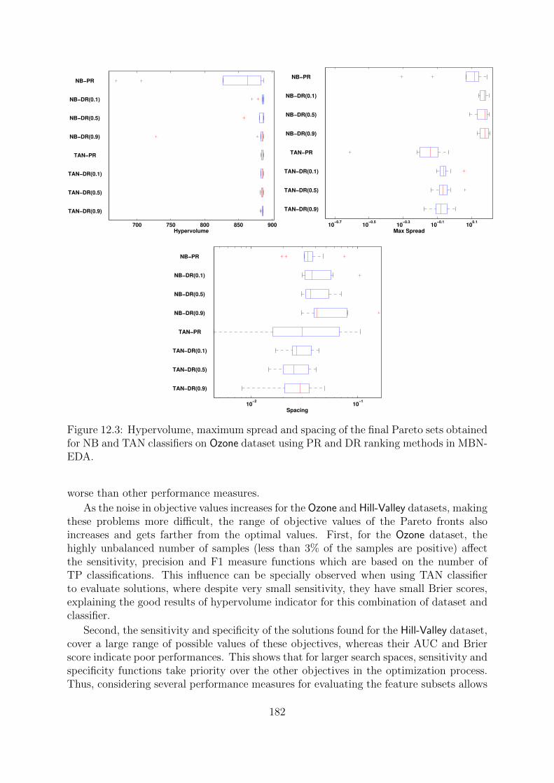
700 750 800 850 900

NB−PR

NB−DR(0.1)

NB−DR(0.5)

NB−DR(0.9)

TAN−PR

TAN−DR(0.1)

TAN−DR(0.5)

TAN−DR(0.9)

Hypervolume10

−0.710

−0.510

−0.310

−0.110

0.1

NB−PR

NB−DR(0.1)

NB−DR(0.5)

NB−DR(0.9)

TAN−PR

TAN−DR(0.1)

TAN−DR(0.5)

TAN−DR(0.9)

Max Spread

10−2

10−1

NB−PR

NB−DR(0.1)

NB−DR(0.5)

NB−DR(0.9)

TAN−PR

TAN−DR(0.1)

TAN−DR(0.5)

TAN−DR(0.9)

Spacing

Figure 12.3: Hypervolume, maximum spread and spacing of the final Pareto sets obtainedfor NB and TAN classifiers on Ozone dataset using PR and DR ranking methods in MBN-EDA.

worse than other performance measures.

As the noise in objective values increases for the Ozone and Hill-Valley datasets, makingthese problems more difficult, the range of objective values of the Pareto fronts alsoincreases and gets farther from the optimal values. First, for the Ozone dataset, thehighly unbalanced number of samples (less than 3% of the samples are positive) affectthe sensitivity, precision and F1 measure functions which are based on the number ofTP classifications. This influence can be specially observed when using TAN classifierto evaluate solutions, where despite very small sensitivity, they have small Brier scores,explaining the good results of hypervolume indicator for this combination of dataset andclassifier.

Second, the sensitivity and specificity of the solutions found for the Hill-Valley dataset,cover a large range of possible values of these objectives, whereas their AUC and Brierscore indicate poor performances. This shows that for larger search spaces, sensitivity andspecificity functions take priority over the other objectives in the optimization process.Thus, considering several performance measures for evaluating the feature subsets allows

182

350 400 450 500 550 600 650 700 750 800

NB−PR

NB−DR(0.1)

NB−DR(0.5)

NB−DR(0.9)

TAN−PR

TAN−DR(0.1)

TAN−DR(0.5)

TAN−DR(0.9)

Hypervolume10

−0.410

−0.210

010

0.2

NB−PR

NB−DR(0.1)

NB−DR(0.5)

NB−DR(0.9)

TAN−PR

TAN−DR(0.1)

TAN−DR(0.5)

TAN−DR(0.9)

Max Spread

10−2

10−1

NB−PR

NB−DR(0.1)

NB−DR(0.5)

NB−DR(0.9)

TAN−PR

TAN−DR(0.1)

TAN−DR(0.5)

TAN−DR(0.9)

Spacing

Figure 12.4: Hypervolume, maximum spread and spacing of the final Pareto sets obtainedfor NB and TAN classifiers on Hill-Valley dataset using PR and DR ranking methods inMBN-EDA.

400 600 800 1000

NB−PR

NB−DR(0.1)

NB−DR(0.5)

NB−DR(0.9)

TAN−PR

TAN−DR(0.1)

TAN−DR(0.5)

TAN−DR(0.9)

Time (seconds)

Figure 12.5: Average solution ranking time in each generation of MBN-EDA with PRand DR ranking methods.

183

Table 12.3: The range of objective values of the solutions in the aggregated Pareto set,obtained from the union of the final Pareto sets of 10 independent MBN-EDA runs, forthe three considered datasets.

WDBC fAUC fsens fspec fprec fF1 fBrier

NB-PRMin. 0.974 0.897 0.958 0.917 0.912 0.038

Max. 0.998 0.970 0.994 0.990 0.961 0.111

NB-DR(0.1)Min. 0.978 0.864 0.948 0.920 0.903 0.068

Max. 0.991 0.937 0.989 0.980 0.944 0.097

NB-DR(0.5)Min. 0.980 0.911 0.968 0.936 0.923 0.054

Max. 0.987 0.955 0.984 0.967 0.954 0.084

NB-DR(0.9)Min. 0.979 0.920 0.957 0.924 0.925 0.059

Max. 0.991 0.941 0.989 0.982 0.954 0.090

TAN-PRMin. 0.958 0.838 0.912 0.851 0.856 0.077

Max. 0.994 0.958 0.978 0.957 0.940 0.166

TAN-DR(0.1)Min. 0.966 0.875 0.918 0.856 0.863 0.085

Max. 0.988 0.944 0.961 0.935 0.936 0.154

TAN-DR(0.5)Min. 0.969 0.874 0.903 0.848 0.861 0.081

Max. 0.988 0.937 0.972 0.952 0.940 0.179

TAN-DR(0.9)Min. 0.976 0.880 0.924 0.891 0.896 0.030

Max. 0.996 0.979 0.990 0.981 0.979 0.132

Ozone fAUC fsens fspec fprec fF1 fBrier

NB-PRMin. 0.763 0.000 0.807 0.000 0.000 0.054

Max. 0.902 0.696 1.000 0.700 0.350 0.341

NB-DR(0.1)Min. 0.720 0.000 0.818 0.000 0.000 0.048

Max. 0.919 0.783 1.000 0.433 0.360 0.309

NB-DR(0.5)Min. 0.793 0.000 0.798 0.000 0.000 0.052

Max. 0.916 0.674 1.000 0.527 0.314 0.364

NB-DR(0.9)Min. 0.777 0.000 0.824 0.000 0.000 0.054

Max. 0.922 0.748 1.000 0.662 0.423 0.309

TAN-PRMin. 0.686 0.000 0.992 0.000 0.000 0.051

Max. 0.861 0.092 1.000 0.467 0.124 0.073

TAN-DR(0.1)Min. 0.721 0.000 0.990 0.000 0.000 0.052

Max. 0.845 0.164 1.000 0.467 0.208 0.076

TAN-DR(0.5)Min. 0.757 0.000 0.989 0.000 0.000 0.054

Max. 0.842 0.130 1.000 0.600 0.157 0.070

TAN-DR(0.9)Min. 0.690 0.000 0.991 0.000 0.000 0.052

Max. 0.874 0.096 1.000 0.467 0.140 0.077

Hill-Valley fAUC fsens fspec fprec fF1 fBrier

NB-PRMin. 0.465 0.073 0.228 0.317 0.118 0.526

Max. 0.546 0.741 0.903 0.591 0.548 0.904

NB-DR(0.1)Min. 0.461 0.000 0.057 0.000 0.000 0.500

Max. 0.543 0.924 1.000 0.594 0.641 0.933

NB-DR(0.5)Min. 0.449 0.000 0.082 0.000 0.000 0.500

Max. 0.541 0.899 1.000 0.585 0.621 0.932

NB-DR(0.9)Min. 0.438 0.000 0.000 0.000 0.000 0.500

Max. 0.546 1.000 1.000 0.578 0.675 0.945

TAN-PRMin. 0.488 0.343 0.346 0.457 0.387 0.513

Max. 0.591 0.723 0.665 0.598 0.617 0.605

TAN-DR(0.1)Min. 0.444 0.000 0.000 0.000 0.000 0.501

Max. 0.581 1.000 1.000 0.573 0.690 0.682

TAN-DR(0.5)Min. 0.480 0.000 0.000 0.000 0.000 0.500

Max. 0.582 1.000 1.000 0.579 0.685 0.690

TAN-DR(0.9)Min. 0.462 0.000 0.000 0.000 0.000 0.499

Max. 0.575 1.000 1.000 0.576 0.685 0.697

184

Features

5 10 15 20 25 30

NB−PR

NB−DR(0.1)

NB−DR(0.5)

NB−DR(0.9)

TAN−PR

TAN−DR(0.1)

TAN−DR(0.5)

TAN−DR(0.9)0

0.5

1

(a) WDBCFeatures

10 20 30 40 50 60 70

NB−PR

NB−DR(0.1)

NB−DR(0.5)

NB−DR(0.9)

TAN−PR

TAN−DR(0.1)

TAN−DR(0.5)

TAN−DR(0.9)0

0.5

1

(b) Ozone

Features

10 20 30 40 50 60 70 80 90 100

NB−PRNB−DR(0.1)NB−DR(0.5)NB−DR(0.9)

TAN−PRTAN−DR(0.1)TAN−DR(0.5)TAN−DR(0.9)

0

0.5

1

(c) Hill-Valley

Figure 12.6: The rate of selecting each feature in the solutions of the final Pareto setsapproximated for NB and TAN classifiers on the three considered datasets using differentranking methods in MBN-EDA. The rates are averaged over 10 independent runs.

us to inspect the final solutions from different points of view, which would not be possiblewhen using only one or two objectives.

12.5.3 Comparison with GA

To evaluate the proposed joint model estimation in MBN-EDA, we compare it with astandard multi-objective GA (MGA), similar to the EMO algorithms reviewed in Section12.2, and study their optimization performance for FSS. Since the recombination oper-ators used in MGA do not require a large population as in the probabilistic modelingof MBN-EDA, we have set the population size of MGA to N = 300 and allowed thealgorithm to evolve for more generations by setting the maximum number of generationsto 350. Thus, while MGA and MBN-EDA are using two different strategies for evolution,both of them have access to similar resources when considering the maximum number offunction evaluations. MGA considered in the experiments employs a two-point crossoverand bit-flip mutation with probabilities Pcross = 0.8 and Pmut = 1/n, respectively. Therest of parameters like the selection ratio are set similar to MBN-EDA as described inthe previous section.

Figures 12.7–12.9 compare the final Pareto sets approximated by MGA and MBN-EDA on each of the three datasets when using the NB classifier, with respect to differentquality indicators. Very similar results are also obtained for the TAN classifier. Thefigures show that the Pareto sets found by MBN-EDA are better than or comparable tothose obtained by MGA on all datasets according to all quality indicators. Especially, forthe WDBC and Ozone datasets, the hypervolume of the Pareto fronts approximated byMBN-EDA is considerably better. This indicates that, although MBN-EDA evolves infewer generations, it is able to perform a more effective search using its joint probabilistic

185

500 550 600 650 700 750 800 850 900

GA−PR

GA−DR(0.1)

GA−DR(0.5)

GA−DR(0.9)

MBN−PR

MBN−DR(0.1)

MBN−DR(0.5)

MBN−DR(0.9)

Hypervolume10

−0.910

−0.710

−0.510

−0.310

−0.1

GA−PR

GA−DR(0.1)

GA−DR(0.5)

GA−DR(0.9)

MBN−PR

MBN−DR(0.1)

MBN−DR(0.5)

MBN−DR(0.9)

Max Spread

0 0.02 0.04 0.06 0.08 0.1 0.12

GA−PR

GA−DR(0.1)

GA−DR(0.5)

GA−DR(0.9)

MBN−PR

MBN−DR(0.1)

MBN−DR(0.5)

MBN−DR(0.9)

Spacing

Figure 12.7: Hypervolume, maximum spread and spacing of the final Pareto sets approx-imated for WDBC dataset with NB classifier, using MGA and MBN-EDA (denoted asMBN).

modeling.

Furthermore, these figures show that the Pareto sets found by MGA using the DRmethod have better hypervolume values than those found using the PR method, whenconsidering the overall behavior on all datasets. This suggests that, in spite of the methodused to explore the search space, the solution ranking provided by DR method can oftenhelp to converge to better Pareto fronts in the noisy FSS problem.

12.5.4 Analysis of Joint Probabilistic Modeling

In this section, the two constituent parts of the joint probabilistic modeling in MBN-EDAare studied during evolution. We are especially interested in the information encoded inthe model about the intrinsic properties of each of the FSS problems. For this purpose,we consider the models estimated using the DR method with a dominance degree ofα = 0.9. First, the set of variables selected in the first part of joint model estimationusing RRMs are examined. Figure 12.10 shows the selected variables during different

186

0 100 200 300 400 500 600 700 800 900

GA−PR

GA−DR(0.1)

GA−DR(0.5)

GA−DR(0.9)

MBN−PR

MBN−DR(0.1)

MBN−DR(0.5)

MBN−DR(0.9)

Hypervolume10

−0.810

−0.610

−0.410

−0.210

010

0.2

GA−PR

GA−DR(0.1)

GA−DR(0.5)

GA−DR(0.9)

MBN−PR

MBN−DR(0.1)

MBN−DR(0.5)

MBN−DR(0.9)

Max Spread

0 0.05 0.1 0.15 0.2 0.25 0.3 0.35 0.4 0.45

GA−PR

GA−DR(0.1)

GA−DR(0.5)

GA−DR(0.9)

MBN−PR

MBN−DR(0.1)

MBN−DR(0.5)

MBN−DR(0.9)

Spacing

Figure 12.8: Hypervolume, maximum spread and spacing of the final Pareto sets approx-imated for Ozone dataset with NB classifier, using MGA and MBN-EDA (denoted asMBN).

generations of evolution, for the tested datasets and classifiers. It can be seen thatfor NB classifier, initially most of the variables are selected in the individuals and duringevolution, gradually the set of the chosen variables becomes smaller (except for Hill-Valleydataset which does not exactly follow this pattern). On the contrary, for TAN classifierthe variable selection frequency usually increases over time.

Here, the selection frequency of variables determines their relevance to the compu-tation of objective values. Unlike the feature selection frequency obtained from the so-lutions, this relevance is not affected only by a certain value (e.g. a zero value) of thevariables. In other words, both inclusion and exclusion of a specific feature influence theapproximation of its relevance to the objectives.

Another part of the study considers the MBN structures estimated in the second partof joint modeling algorithm. As it is expected and explained in Section 10.6, considerablymore arcs are added to the class and bridge subgraphs of MBN (i.e. between objectivesand between variables and objectives) than to the feature subgraph, indicating the im-portance of these relations. Here, we depict only the class subgraphs of the estimated

187

0 100 200 300 400 500 600 700 800

GA−PR

GA−DR(0.1)

GA−DR(0.5)

GA−DR(0.9)

MBN−PR

MBN−DR(0.1)

MBN−DR(0.5)

MBN−DR(0.9)

Hypervolume10

−0.610

−0.410

−0.210

010

0.2

GA−PR

GA−DR(0.1)

GA−DR(0.5)

GA−DR(0.9)

MBN−PR

MBN−DR(0.1)

MBN−DR(0.5)

MBN−DR(0.9)

Max Spread

0 0.1 0.2 0.3 0.4 0.5

GA−PR

GA−DR(0.1)

GA−DR(0.5)

GA−DR(0.9)

MBN−PR

MBN−DR(0.1)

MBN−DR(0.5)

MBN−DR(0.9)

Spacing

Figure 12.9: Hypervolume, maximum spread and spacing of the final Pareto sets approx-imated for Hill-Valley dataset with NB classifier, using MGA and MBN-EDA (denoted asMBN).

MBNs to preserve the space. Figure 12.11 shows the overall frequency of arcs in the classsubgraph of the estimated MBN structures in all generations of MBN-EDA and in 10independent runs, for the tested datasets and classifiers.

It can be seen that certain patterns of interaction between objectives have a higherfrequency of occurrence in FSS on the tested datasets. These include the dependenciesbetween sensitivity, specificity and precision, between AUC and Brier score, and betweensensitivity and F1 function. Some of these relationships can be easily approved by lookingat the definitions of objective functions in Equation (12.4). For example, F1 measure isthe harmonic mean of sensitivity and precision, and thus any information on the value ofone of these objectives can be used to approximate the value of the other.

An interesting observation is the role of classifiers in detecting the interactions betweenobjectives. It seems that the proposed joint model estimation is able to identify thesekind of relationships better when the TAN classifier is used for solution evaluation. Oneexplanation for this behavior is that for the TAN classifier the sets of variables selected inthe first part of model learning using RRMs are smaller, especially at the early generations

188

NB−DR(0.9)

Features

Ge

ne

rati

on

s

5 10 15 20 25 30

1

10

20

30

40

500

0.5

1

NB−DR(0.9)

Features

Gen

era

tio

ns

10 20 30 40 50 60 70

1

10

20

30

40

500

0.5

1

TAN−DR(0.9)

Features

Ge

ne

rati

on

s

5 10 15 20 25 30

1

10

20

30

40

500

0.5

1

(a) WDBC

TAN−DR(0.9)

Features

Gen

era

tio

ns

10 20 30 40 50 60 70

1

10

20

30

40

500

0.5

1

(b) Ozone

NB−DR(0.9)

Features

Gen

era

tio

ns

10 20 30 40 50 60 70 80 90 100

1

10

20

30

40

500

0.5

1

TAN−DR(0.9)

Features

Gen

era

tio

ns

10 20 30 40 50 60 70 80 90 100

1

10

20

30

40

500

0.5

1

(c) Hill-Valley

Figure 12.10: The average frequency of selecting variables using RRMs in the first part ofjoint model estimation, along different generations of MBN-EDA and in 10 independentruns.

of the evolution, where the algorithm is detecting the direction of movement in the searchspace. This allows to filter out variables that would introduce noise to the MBN inductionprocess, which in turn helps to detect the relationships between objectives.

For some of the problem instances under study, the probability of recovering therelationships between objectives in the joint probabilistic model is very low. This situationcan be observed for Ozone dataset with TAN classifier (bottom-middle of Figure 12.11)and Hill-Valley dataset with NB classifier (top-right of Figure 12.11). These cases showtwo possible situations where objective relationships are not considered to be important

189

NB−DR(0.9)

AUC

sens

spec

prec F1

Brie

r

AUC

sens

spec

prec

F1

Brier

0

0.2

0.4

0.6

0.8

1NB−DR(0.9)

AUC

sens

spec

prec F1

Brie

r

AUC

sens

spec

prec

F1

Brier

0

0.2

0.4

0.6

0.8

1NB−DR(0.9)

AUC

sens

spec

prec F1

Brie

r

AUC

sens

spec

prec

F1

Brier

0

0.2

0.4

0.6

0.8

1

TAN−DR(0.9)

AUC

sens

spec

prec F1

Brie

r

AUC

sens

spec

prec

F1

Brier

0

0.2

0.4

0.6

0.8

1

(a) WDBC

TAN−DR(0.9)

AUC

sens

spec

prec F1

Brie

r

AUC

sens

spec

prec

F1

Brier

0

0.2

0.4

0.6

0.8

1

(b) Ozone

TAN−DR(0.9)

AUC

sens

spec

prec F1

Brie

r

AUC

sens

spec

prec

F1

Brier

0

0.2

0.4

0.6

0.8

1

(c) Hill-Valley

Figure 12.11: The average frequency of arcs in the class subgraph of the MBNs estimatedin all generations of MBN-EDA and in 10 independent runs.

for optimization by MBN-EDA. In the latter case, most of the variables are selectedfor inclusion in MBN estimation by the first part of joint modeling algorithm, in allgenerations (see Figure 12.10). As it was already explained, this directly affects thedetection of relationships in the class subgraph. In the former case, although a relativelysmaller number of variables are selected for inclusion in MBN, the high level inconsistencyof the objective values due to noise (especially with the unbalanced dataset) makes it hardfor the MBN induction algorithm to detect any interactions.

12.6 Conclusions

An adaptation of MBN-EDA for FSS problem based on joint modeling of variables andobjectives, when the noise in objective values is represented as intervals was proposed inthis chapter. The algorithm was applied for FSS in classification, although the methodcan be easily adapted for FSS in clustering. To deal with the inherent noise in theestimation of objective values, the proposed algorithm employs a ranking method that isable to order the solutions in the population when objective values are given as intervals.Based on this ordering, a subset of promising solutions were selected for model estimation.

A two-step learning method was proposed for estimating a joint probabilistic model ofvariables and objectives from the selected solutions. In the first step, the variable selectionproperty of `1-regularization technique was employed to select a subset of variables withhigher relevance to the objectives. This helped to simplify MBN estimation by reducing

190

the space of possible structures and provided an initial approximation of the bridgesubgraph structure of MBN. In the second step, an MBN was estimated encoding theobjectives and the set of selected variables.

We defined a six objective optimization problem and used the proposed algorithm toselect feature subsets for two Bayesian classifiers, NB and TAN, in three different datasetshaving an increasing number of features. The experimental results showed that, althoughrequiring considerably less time, the Pareto sets approximated with the proposed DRmethod were comparable or better than the Pareto sets found using the well-known PRmethod. Moreover, the comparison of results with those of a standard multi-objectiveGA showed that the proposed algorithm is able to obtain better Pareto sets in terms ofboth convergence and diversity.

The estimated joint probabilistic models were also used to analyze the interactionsbetween objectives and variables. We saw different variable selection behaviors with eachof the classifiers which resulted in detecting different patterns of objective interactions. Itwas observed that, though the level of noise in the objective values is higher when usingTAN classifier for solution evaluation, the variable selection method deployed in the firstpart of the model estimation can identify these relationships.

191

192

Part IV

Conclusions

193

Chapter 13

Conclusions and Future Lines ofResearch

In this section, we first review the work presented throughout this thesis, and then listthe main results of our study. At the end, we also give some lines of future researchregarding the presented work. The main contributions of the thesis are summarized inTable 13.1.

13.1 Thesis Overview

The inherent properties of EDAs and the way they solve optimization problems makethem very interesting, and though they are a relatively new class of EAs, many workshave studied these algorithms from both theoretical and application-based points of view,and they are still topic of active research. Probabilistic modeling, which is the essentialpart of EDAs, is one of the topics that requires further and a more thorough investiga-tion. In this thesis, we proposed and studied the use of regularization techniques in themodel estimation of EDAs as a promising method for both continuous and multi-objectiveoptimization.

Two main approaches for regularized model learning in EDAs was presented in Chap-ter 5. In the first approach, an estimation of the model structure is obtained by explicitlyusing regularization to capture the dependencies between variables, and then the modelparameters are estimated separately. In the second approach, regularization techniquesare applied to obtain an estimation of the probabilistic model, which is an MGD. Theproposed methods were analyzed considering different aspects when used for estimatingmodels from the populations generated by sampling a number of Gaussian models withan increasing level of interactions between the variables. The resulting RegEDA wasthen applied to continuous function optimization with a high-dimensional setting for itspopulation size in Chapter 6, and the achieved results were analyzed by comparing themwith those of several other well-known Gaussian-based EDAs.

We then used `1-regularized modeling for obtaining a decomposition of problem vari-ables in Chapter 7, and to learn a marginally factorized probability distribution encodedin a GMRF model. The proposed algorithm first identifies the (in)dependencies betweenvariables and then uses their interaction strengths to divide the variables into a numberof disjoint groups with the AP clustering algorithm which can automatically identify the

195

Table 13.1: A summary of the contributions and algorithms proposed in the thesis andtheir domains of application.

Single-ObjectiveMulti-Objective

Noiseless NoisyContinuous Discrete

Algorithm RegEDA GMRF-EDA JGBN-EDA MBN-EDA

ProbabilisticModel

MGD/GMRFMarginallyFactorized

GMRFBN MBN

ProposalRegularized

ModelLearning

RegularizedDecomposition

Learning

Joint Variable-Objective Modelingα-Degree Pareto

Dominance BasedRanking

RegularizedStructureLearning

• • •

RegularizedParameterLearning

• • • •

Chapter 5, 6 7 9 10 11 12

Publication[Karshenas

et al., 2013b][Karshenas

et al., 2012a][Karshenas

et al., 2011b][Karshenas

et al., 2012b][Karshenas

et al., 2013a]

number of clusters. The behavior of GMRF-EDA was then tested on a continuous addi-tively decomposable function and two instances of the off-lattice protein folding model.

In Chapter 9, joint variable-objective probabilistic modeling was proposed as a novelapproach for multi-objective optimization with EDAs. We presented methods for learningand sampling the joint probabilistic model, which was encoded in a BN. Specifically, incontinuous domains we used a regularized estimation of GBN to address the increaseddimensionality due to the inclusion of objectives in the joint probabilistic model. Theproposed JGBN-EDA was then compared against a similar GBN-based EDA, which doesnot consider objectives in its probabilistic model, on a set of benchmark MOPs to studythe effect of incorporating the objective values in probabilistic modeling of multi-objectiveEDAs.

This study was further extended in Chapter 10 by using MBNs for encoding threetypes of interactions in the joint probabilistic models and specific solution ranking meth-ods proposed in the literature for many-objective optimization. The performance of theresulting algorithm, which is called MBN-EDA, was tested in an extensive experimentalstudy on two sets of benchmark MOPs with different number of objectives, and com-pared with several other state-of-the-art algorithms. Moreover, we took a closer look atthe joint probabilistic models estimated in MBN-EDA and analyzed the ability of thisalgorithm to approximate the MOP structure.

In Chapter 11, the α-degree Pareto dominance relation was defined to deal withthe noise in the objective values of MOPs, given as intervals. We studied some of theproperties of this dominance relation when noisy objective values are given as confidenceintervals, and used it to develop a modified version of the non-dominated sorting algorithmfor ranking the solutions in the presence of noise in the objective values. This rankingmethod was compared to probabilistic ranking, a widely used noise handling method

196

in EMO algorithm which can also be applied to objective values given as intervals, tooptimize a set of noisy MOPs with three different levels of Gaussian noise using MBN-EDA.

Finally in Chapter 12, we proposed a version of MBN-EDA for multi-objective FSSin classification, when several measures of classification performance are considered asobjectives. The different quality values obtained in the cross-validation evaluation of thefeature subsets were used to compute confidence intervals as the objective values, and adegree ranking method based on the α-degree Pareto dominance was proposed to order thesolutions. To learn a joint variable-objective probabilistic model, a two-step estimationapproach was proposed. In the first step, `1-regularization is used to identify the variablesrelated to each objective, and a subset of variables which have more interactions withthe objective are selected. In the second step, a joint model of objectives and selectedvariables is estimated in an MBN, and marginal univariate probability distributions areestimated for the rest of variables. The resulting algorithm was then tested on a number ofdatasets with increasing number of features, when using two different Bayesian classifier,and its constituent parts for solution ranking and reproduction were compared with othercommonly used methods. The estimated model structures during evolution on each testeddataset-classifier combination were also analyzed.

The discussions in the thesis covered a broad range of topics in a variety of domainsand applications. Therefore, to introduce the context of study, the main concepts and theproposed methods and approaches were reviewed in each case. This reviews include: twomain types of PGMs, probabilistic modeling in EAs, BN learning and inference relatedoptimization problems solved with EAs, regularization techniques for estimating differ-ent types of models, multi-objective EDAs and their ranking methods and probabilisticmodels, methods for noisy optimization with EMO algorithms, and the methods used formulti-objective FSS in classification and clustering with EMO algorithms.

13.2 Main Results

Although we have given some conclusions at the end of each chapter, summarizing thecontributions and achievements, there are a number of conclusions that can be pointedout as the main results of the research conducted in this thesis. Following the organizationof the thesis, these findings can be divided into two parts. Regarding continuous functionoptimization with EDAs, the main results are:

• The analysis of the proposed methods for regularized model estimation with high-dimensional settings for the population showed the usefulness of each techniquefor continuous optimization of a different type of problem with EDAs. Some ofthe methods are able to detect many interactions in a short time, whereas othersrequire more time to obtain sparser model estimations. It was shown that the levelof sparsity of the interactions between problem variables can decrease the qualityof the models obtained with regularized estimation.

• We tested RegEDA with different methods for regularized model estimation oncontinuous problems with an increasing number of variables in a high-dimensionalsetting, simulated with a population size that is logarithmic in the number of vari-

197

ables. The optimization results showed that because of the robust model estima-tion based on regularization, RegEDA is less affected by the curse of dimensionalityphenomenon in comparison to several other Gaussian-based EDAs, and is able toachieve significantly better results on larger dimensions of many of the tested con-tinuous functions.

• The variable selection property of `1-regularization can be a promising approachfor linkage learning in EDAs. The method we proposed based on this type ofregularization for estimating a marginally factorized probability distribution, oftenknown as MPM in EDA literature, was shown to be more effective than estimatingnon-marginal factorized models or models with complete variable independenceassumption, in the optimization of continuous additively decomposable problems.

The above results also apply to EDAs used for multi-objective optimization. Yet,there are a number of interesting findings in our study of multi-objective optimizationwith EDAs:

• Incorporating information about objectives into model estimation and sampling ofEDAs proved to be useful for a more effective multi-objective optimization, andallowed achieving significantly better results on several MOPs in comparison toother EMO algorithms that ignore this kind of information when generating newsolutions. The proposed joint variable-objective probabilistic modeling approachprovides a systematic way for modeling the relationships between objectives whichis often needed for many-objective optimization. We showed that with this typeof model estimation, the resulting EDA is also able to implicitly obtain a goodapproximation of the MOP structure in a probabilistic framework, which can be aninteresting alternative to a set of solutions for DMs.

• The study of the estimated probabilistic models showed that the two new typesof interactions captured as a result of joint variable-objective modeling, which arethe objective-variable and objective-objective relationships, are considerably moreimportant for multi-objective optimization than the variable-variable relationshipsusually modeled in other EDAs.

• It was shown that α-degree Pareto dominance proposed for solution ordering innoisy multi-objective optimization, when objective values are given as intervals, de-fines a partial relation between the solutions in the search space. Moreover, whennoisy objective values are represented as confidence intervals, it was demonstratedthat any reduction in the minimum acceptable dominance degree or confidencelevel does not affect the α-degree Pareto dominance relation between the solutions.We showed that the Pareto set approximations obtained using two solution rank-ing methods based on this dominance relation are better or comparable to thoseobtained by a standard solution ranking method while having a considerably lesscomputational complexity.

• Relatively good feature subsets can be found in a small number of generationswhen using multi-objective EDAs for FSS in classification problems. This approachto FSS is more effective for datasets with small-medium dimensionality, due to

198

the large populations required for datasets with a large number of features. Theregularization-based joint probabilistic modeling in this problem allows to obtainan estimation of how different measures of classification performance are related.

13.3 Future Lines of Research

There are a number of possibilities for continuing the research carried out in this thesis.In this section we give some hints for further extension of our study of EDAs in continuousand multi-objective optimization.

Continuous optimization has specific properties that makes it very different fromdiscrete optimization of combinatorial problems. For example, a single variable may havea global optimal value with a small basin of attraction and many deceptive local optima.One of the approaches used to improve continuous optimization is the incorporation ofgradient information in the search. This allows the optimization algorithm to adapt tothe landscape of the problem at hand and increase or decrease its pace. CMA-ES is oneof the successful continuous EDAs that has employed this approach. However, as it wasshown in Chapter 6, this adaption considerably affects the performance of this algorithmon problems with large dimensionality. On the other hand, regularized model estimationoffers a method for learning models with better generalization ability. An interesting lineof future research is to combine these two approaches of model estimation for continuousoptimization with EDAs. A starting point for this study is to decompose the problem anduse an adapted model learning in the subspaces while controlling the overall fitting of themodels with regularized estimation. The variable selection property of `1-regularizationcan be especially useful for this purpose. Such an approach is specifically applicable tohigh-dimensional problems where decomposition becomes necessary for the feasibility andefficiency of the optimization with EDAs.

Another future work of regularized model estimation in EDAs is to explicitly considernonlinear interactions between variables when learning their relationships. A preliminarystudy of this type of regularized model estimation for learning discrete MNs was presentedin [Santana et al., 2011]. The emergence of new techniques in the statistics communityfor efficient regularized learning of GGMs considering higher order relationships betweenvariables can be useful in this respect. A closely related topic for further research is touse non-Gaussian assumptions for the variables when obtaining regularized estimationsof their relationships.

With the proposed approach for multi-objective optimization based on joint variable-objective modeling, the estimated models encode probabilistic estimations for the valuesof both variables and objectives. We used these probabilistic estimations to generatenew values for the variables. A future line of research is to analyze the optimizationperformance when the encoded probabilistic estimations are also used to approximatethe objective values of the newly generated solutions. Such an approach can be taken,for example, when optimizing MOPs with expensive (e.g. computationally or economi-cally) objective functions [Zhang et al., 2010]. A related future study is to exploit therelationships encoded as a result of objective modeling to reduce the cost of solutionevaluation in multi-objective optimization. For example in multi-objective FSS, a combi-nation of filter-based and wrapper-based objectives can be considered. Then, depending

199

on the objective relationships encoded in the joint probabilistic model, the value of thewrapper-based objectives for the new solutions can be approximated using the estimatedmodel and only the considerably cheaper filter-based objectives need to be evaluated ineach generation.

The application of the methods proposed in the thesis to real-world problems is alsoa potential future work. There are several problems like gene expression analysis in ge-nomics [Bielza et al., 2008] and optimal ordering of tables in text organization [Bengoetxeaet al., 2011] which are characterized by high-dimensionality, involving optimization overa large number of variables. Regularization-based EDAs are promising methods for thistype of problems. In multi-objective optimization, an interesting research is to evaluatethe MOP structures estimated with joint probabilistic modeling for real-world problemsagainst DM’s knowledge of the problem. Moreover, preference information of DMs canbe incorporated into joint probabilistic modeling to improve optimization performance ofthe algorithm [di Pierro et al., 2007; Hirsch et al., 2011]. It can be used as conditionalindependence relations between objectives and variables, or inserted as preferable valuesfor the objectives.

200

Appendix A

List of Abbreviations

AIC Akaike’s Information CriterionANN Artificial Neural NetworkANOVA Analysis Of VarianceAP Affinity PropagationAUC Area Under ROC CurveBAV Best Achieved ValueBDe Bayesian Dirichlet equivalenceBIC Bayesian Information CriterionBN Bayesian NetworkCGN Conditional Gaussian Bayesian NetworkDAG Directed Acyclic GraphDAGS DAG SearchDBN Dynamic Bayesian NetworkDM Decision MakerDR Degree RankingDT Decision TreeEA Evolutionary AlgorithmEDA Estimation of Distribution AlgorithmEM Expectation MaximizationEMO Evolutionary Multi-objective OptimizationEP Evolutionary ProgrammingES Evolutionary StrategyFSS Feature Subset SelectionGA Genetic AlgorithmGBN Gaussian Bayesian NetworkGGM Gaussian Graphical ModelGMRF Gaussian Markov Random FieldGP Genetic ProgrammingIGD Inverted Generational DistancekDB k-Dependence Bayesian ClassifierMAP Maximum A PosterioriMCMC Markov Chain Monte Carlo

201

MB Markov BlanketMBN Multi-dimensional Bayesian NetworkMDL Minimum Description LengthMGD Multivariate Gaussian DistributionML Maximum LikelihoodMN Markov NetworkMOP Multi-objective Optimization ProblemMPE Most Probable ExplanationMPM Marginal Product ModelMTE Mixture of Truncated ExponentialsNB Naıve Bayes ClassifierNLL Negative Log-LikelihoodNN Nearest NeighborPDAG Partial Directed Acyclic GraphPGM Probabilistic Graphical ModelPLS Probabilistic Logic SamplingPR Probabilistic RankingPSO Particle Swarm OptimizationRRM Regularized Regression ModelSNB Semi-Naıve Bayes ClassifierSVM Support Vector MachineTAN Tree Augmented Naıve Bayes ClassifierTSP Traveling Salesman ProblemWFG Walking Fish Group

202

Bibliography

A. Abraham, L. Jain, and R. Goldberg, editors. Evolutionary Multiobjective Optimization:Theoretical Advances and Applications, Springer, Berlin, 2005.

P. Agarwal and C. Procopiuc. Exact and approximation algorithms for clustering. Algo-rithmica, 33(2):201–226, 2002.

H. Aguirre and K. Tanaka. A study on the effects of rankings sensitive to density onmany-objective MNK landscapes. In IEEE Congress on Evolutionary Computation(CEC’10), IEEE World Congress on Computational Intelligence (WCCI 2010), pages1089–1096, 2010.

C. Ahn, R. Ramakrishna, and D. Goldberg. Real-coded Bayesian optimization algorithm:Bringing the strength of BOA into the continuous world. In Sixth Annual Conference onGenetic and Evolutionary Computation (GECCO ’04), volume 3102 of Lecture Notesin Computer Science, pages 840–851. Springer, 2004.

C. W. Ahn and R. S. Ramakrishna. Multiobjective real-coded Bayesian optimizationalgorithm revisited: Diversity preservation. In 9th Annual Conference on Genetic andEvolutionary Computation (GECCO ’07), pages 593–600. ACM, 2007.

C. W. Ahn, J. An, and J.-C. Yoo. Estimation of particle swarm distribution algorithms:Combining the benefits of PSO and EDAs. Information Sciences, 192:109–119, 2012.

H. Akaike. A new look at the statistical model identification. IEEE Transactions onAutomatic Control, 19(6):716–723, 1974.

J. T. Alander. An indexed bibliography of genetic algorithms in medicine. TechnicalReport 94-1-MEDICINE, University of Vaasa, Finland, 2012.

M. E. Alden. MARLEDA: Effective Distribution Estimation through Markov RandomFields. PhD thesis, The University of Texas at Austin, 2007.

G. Andrew and J. Gao. Scalable training of l1-regularized log-linear models. In 24thInternational Conference on Machine Learning (ICML ’07), pages 33–40. ACM, 2007.

R. Armananzas, I. Inza, R. Santana, Y. Saeys, J. Flores, J. Lozano, Y. Van de Peer,R. Blanco, V. Robles, C. Bielza, and P. Larranaga. A review of estimation of distribu-tion algorithms in bioinformatics. BioData Mining, 1(6):online, DOI: 10.1186/1756–0381–1–6, 2008.

203

R. Armananzas, Y. Saeys, I. Inza, M. Garcıa-Torres, C. Bielza, Y. van de Peer, andP. Larranaga. Peakbin selection in mass spectrometry data using a consensus ap-proach with estimation of distribution algorithms. IEEE/ACM Transactions on Com-putational Biology and Bioinformatics, 8(3):760–774, 2011.

D. Arnold and H.-G. Beyer. A general noise model and its effects on evolution strategyperformance. IEEE Transactions on Evolutionary Computation, 10(4):380–391, 2006.

M. Babbar, A. Lakshmikantha, and D. E. Goldberg. A modified NSGA-II to solvenoisy multiobjective problems. In Genetic and Evolutionary Computation Conference(GECCO’03), pages 21–27, 2003.

J. Bader and E. Zitzler. HypE: An algorithm for fast hypervolume-based many-objectiveoptimization. Evolutionary Computation, 19(1):45–76, 2011.

S. Baluja. Population-based incremental learning: A method for integrating geneticsearch based function optimization and competitive learning. Technical Report CMU-CS-94-163, Carnegie-Mellon University, Pittsburgh PA, 1994.

S. Baluja and S. Davies. Using optimal dependency-trees for combinational optimiza-tion. In 14th International Conference on Machine Learning, pages 30–38. MorganKaufmann Publishers Inc., 1997.

S. Bandaru and K. Deb. Automated innovization for simultaneous discovery of multiplerules in bi-objective problems. In Evolutionary Multi-Criterion Optimization, volume6576 of Lecture Notes in Computer Science, pages 1–15. Springer, 2011.

O. Banerjee, L. El Ghaoui, and A. d’Aspremont. Model selection through sparse max-imum likelihood estimation for multivariate Gaussian or binary data. The Journal ofMachine Learning Research, 9:485–516, 2008.

O. Barriere, E. Lutton, and P.-H. Wuillemin. Bayesian network structure learning usingcooperative coevolution. In 11th Annual Conference on Genetic and EvolutionaryComputation (GECCO ’09), pages 755–762. ACM, 2009.

M. Basseur and E. Zitzler. Handling uncertainty in indicator-based multiobjective opti-mization. International Journal of Computational Intelligence Research, 2(3):255–272,2006.

A. Beck and Y. Eldar. Regularization in regression with bounded noise: A Chebyshevcenter approach. SIAM Journal on Matrix Analysis and Applications, 29(2):606–625,2008.

E. Bengoetxea and P. Larranaga. EDA-PSO: A hybrid paradigm combining estimationof distribution algorithms and particle swarm optimization. In Swarm Intelligence,volume 6234 of Lecture Notes in Computer Science, pages 416–423. Springer, 2010.

E. Bengoetxea, T. Miquelez, P. Larranaga, and J. Lozano. Experimental results in func-tion optimization with EDAs in continuous domain. In Larranaga and Lozano [2001],chapter 8, pages 181–194.

204

E. Bengoetxea, P. Larranaga, C. Bielza, and J. Fernandez del Pozo. Optimal row andcolumn ordering to improve table interpretation using estimation of distribution algo-rithms. Journal of Heuristics, 17(5):567–588, 2011.

H.-G. Beyer. The Theory of Evolution Strategies, Springer, 2001.

H.-G. Beyer and H.-P. Schwefel. Evolution strategies – comprehensive introduction. Nat-ural Computing, 1:3–52, 2002.

P. Bickel and E. Levina. Regularized estimation of large covariance matrices. Annals ofStatistics, 36(1):199–227, 2008.

C. Bielza, V. Robles, and P. Larranaga. Estimation of distribution algorithms as logisticregression regularizers of microarray classifiers. Methods of Information in Medicine,16:345–366, 2008.

C. Bielza, M. Gomez, and P. P. Shenoy. A review of representation issues and modelingchallenges with influence diagrams. Omega, 39(3):227–241, 2011a.

C. Bielza, G. Li, and P. Larranaga. Multi-dimensional classification with Bayesian net-works. International Journal of Approximate Reasoning, 52(6):705–727, 2011b.

J. Bien and R. J. Tibshirani. Sparse estimation of a covariance matrix. Biometrika, 98(4):807–820, 2011.

M. Bilodeau and D. Brenner. Theory of Multivariate Statistics, Springer-Verlag, 1999.

R. Blanco, I. Inza, and P. Larranaga. Learning Bayesian networks in the space of struc-tures by estimation of distribution algorithms. International Journal of IntelligentSystems, 18(2):205–220, 2003.

R. Blanco, P. Larranaga, I. Inza, and B. Sierra. Gene selection for cancer classificationusing wrapper approaches. International Journal of Pattern Recognition and ArtificialIntelligence, 18(8):1373–1390, 2004.

A. L. Blum and P. Langley. Selection of relevant features and examples in machinelearning. Artificial Intelligence, 97(1–2):245–271, 1997.

P. Boonma and J. Suzuki. A confidence-based dominance operator in evolutionary algo-rithms for noisy multiobjective optimization problems. In 21st International Conferenceon Tools with Artificial Intelligence (ICTAI’09), pages 387–394, 2009.

P. A. Bosman and D. Thierens. Multi-objective optimization with diversity preserv-ing mixture-based iterated density estimation evolutionary algorithms. InternationalJournal of Approximate Reasoning, 31(3):259–289, 2002.

P. A. Bosman and D. Thierens. Numerical optimization with real-valued estimation-of-distribution algorithms. In Pelikan et al. [2006a], chapter 5, pages 91–120.

205

P. A. N. Bosman and E. de Jong. Adaptation of a success story in GAs: Estimation-of-distribution algorithms for tree-based optimization problems. In Success in Evolu-tionary Computation, volume 92 of Studies in Computational Intelligence, pages 3–18.Springer, 2008.

P. A. N. Bosman and J. Grahl. Matching inductive search bias and problem structurein continuous estimation of distribution algorithms. European Journal of OperationalResearch, 185(3):1246–1264, 2008.

P. A. N. Bosman and D. Thierens. Expanding from discrete to continuous estimationof distribution algorithms: The IDEA. In Sixth International Conference on ParallelProblem Solving from Nature (PPSN VI), volume 1917 of Lecture Notes in ComputerScience, pages 767–776. Springer-Verlag, 2000a.

P. A. N. Bosman and D. Thierens. Continuous iterated density estimation evolutionaryalgorithms within the IDEA framework. In Genetic and Evolutionary ComputationConference (GECCO ’00) Workshop, pages 197–200, 2000b.

P. A. N. Bosman and D. Thierens. Advancing continuous IDEAs with mixture distri-butions and factorization selection metrics. In Optimization by Building and UsingProbabilistic Models (OBUPM) Workshop at the Genetic and Evolutionary Computa-tion Conference (GECCO ’01), pages 208–212. ACM, 2001.

P. A. N. Bosman and D. Thierens. Adaptive variance scaling in continuous multi-objectiveestimation of distribution algorithms. In 9th Annual Conference on Genetic and Evo-lutionary Computation (GECCO ’07), pages 500–507. ACM, 2007.

P. A. N. Bosman, J. Grahl, and D. Thierens. Enhancing the performance of maximum–likelihood Gaussian EDAs using anticipated mean shift. In 10th International Con-ference on Parallel Problem Solving from Nature (PPSN X), pages 133–143. Springer,2008.

R. R. Bouckaert. Bayesian Belief Networks: From Construction to Inference. PhD thesis,Universiteit Utrecht, Faculteit Wiskunde en Informatica, 1995.

D. Brockhoff and E. Zitzler. Objective reduction in evolutionary multiobjective optimiza-tion: Theory and applications. Evolutionary Computation, 17(2):135–166, 2009.

A. Brownlee, J. McCall, Q. Zhang, and D. Brown. Approaches to selection and their effecton fitness modelling in an estimation of distribution algorithm. In IEEE Congress onEvolutionary Computation (CEC 2008) – IEEE World Congress on ComputationalIntelligence, pages 2621–2628. IEEE Computer Society, 2008.

A. E. I. Brownlee. Multivariate Markov Networks for Fitness Modelling in an Estima-tion of Distribution Algorithm. PhD thesis, The Robert Gordon University. School ofComputing, 2009.

D. Buche, P. Stoll, R. Dornberger, and P. Koumoutsakos. Multiobjective evolutionaryalgorithm for the optimization of noisy combustion processes. IEEE Transactions onSystems, Man, and Cybernetics, Part C: Applications and Reviews, 32(4):460–473,2002.

206

P. Buhlmann, M. Kalisch, and M. H. Maathuis. Variable selection in high-dimensional lin-ear models: Partially faithful distributions and the PC-simple algorithm. Biometrika,97(2):261–278, 2010.

L. T. Bui, H. A. Abbass, and D. Essam. Fitness inheritance for noisy evolutionarymulti-objective optimization. In Conference on Genetic and Evolutionary Computation(GECCO’05), pages 779–785. ACM, 2005a.

L. T. Bui, D. Essam, H. A. Abbass, and D. Green. Performance analysis of evolutionarymulti-objective optimization methods in noisy environments. Complexity International,11:29–39, 2005b.

L. T. Bui, H. A. Abbass, and D. Essam. Localization for solving noisy multi-objectiveoptimization problems. Evolutionary Computation, 17(3):379–409, 2009.

W. Buntine. Theory refinement on Bayesian networks. In 7th Annual Conference onUncertainty in Artificial Intelligence (UAI ’91), pages 52–60. Morgan Kaufmann, 1991.

W. Buntine. A guide to the literature on learning probabilistic networks from data. IEEETransactions on Knowledge and Data Engineering, 8(2):195–210, 1996.

A. Cano, S. Moral, and A. Salmeron. Novel strategies to approximate probability treesin penniless propagation. International Journal of Intelligent Systems, 18(2):193–203,2003.

G. Casella and E. I. George. Explaining the Gibbs sampler. The American Statistician,46(3):167–174, 1992.

R. Castelo and T. Kocka. On inclusion-driven learning of Bayesian networks. Journal ofMachine Learning Research, 4:527–574, 2003.

E. Castillo, J. M. Gutierrez, and A. S. Hadi. Expert Systems and Probabilistic NetworkModels, Springer, 1997.

F. Chan and S. Chung. Multi-criteria genetic optimization for distribution network prob-lems. The International Journal of Advanced Manufacturing Technology, 24:517–532,2004.

S. Chaudhuri, M. Drton, and T. S. Richardson. Estimation of a covariance matrix withzeros. Biometrika, 94(1):199–216, 2007.

B. Chen and J. Hu. An adaptive niching EDA based on clustering analysis. In IEEECongress on Evolutionary Computation (CEC ’10), pages 1–7, 2010.

S.-H. Chen and M.-C. Chen. Addressing the advantages of using ensemble probabilisticmodels in estimation of distribution algorithms for scheduling problems. InternationalJournal of Production Economics, 141(1):24–33, 2013.

Y. Chen, A. Wiesel, and A. Hero. Robust shrinkage estimation of high-dimensional covari-ance matrices. In IEEE Sensor Array and Multichannel Signal Processing Workshop(SAM ’10), pages 189–192, 2010.

207

J. Cheng, D. Bell, and W. Liu. Learning Bayesian networks from data: An information-theory based approach. Artificial Intelligence, 137(1-2):43–90, 2002.

S. Chib and E. Greenberg. Understanding the Metropolis-Hastings algorithm. The Amer-ican Statistician, 49(4):327–335, 1995.

D. M. Chickering. Learning Bayesian networks is NP-complete. In Learning from Data:Artificial Intelligence and Statistics V, volume 112 of Lecture Notes in Statistics, pages121–130. Springer, 1996.

D. M. Chickering. Learning equivalence classes of Bayesian-network structures. Journalof Machine Learning Research, 2:445–498, 2002.

D. M. Chickering, D. Geiger, and D. Heckerman. Learning Bayesian networks is NP-hard.Technical Report MSR-TR-94-17, Microsoft Research, Redmond, WA, USA, 1994.

D. M. Chickering, D. Heckerman, and C. Meek. Large-sample learning of Bayesian net-works is NP-hard. Journal of Machine Learning Research, 5:1287–1330, 2004.

D.-Y. Cho and B.-T. Zhang. Evolutionary optimization by distribution estimation withmixtures of factor analyzers. In IEEE Congress on Evolutionary Computation (CEC’02), volume 2, pages 1396–1401. IEEE Computer Society, 2002.

D.-Y. Cho and B.-T. Zhang. Evolutionary continuous optimization by distribution esti-mation with variational Bayesian independent component analyzers mixture model. InParallel Problem Solving from Nature (PPSN VIII), volume 3242 of Lecture Notes inComputer Science, pages 212–221. Springer, 2004.

C. A. Coello Coello and N. C. Cortes. Solving multiobjective optimization problemsusing an artificial immune system. Genetic Programming and Evolvable Machines, 6:163–190, 2005.

C. A. Coello Coello, G. B. Lamont, and D. A. Van Veldhuizen. Evolutionary Algorithmsfor Solving Multi-Objective Problems, Springer, second edition, 2007.

G. Cooper and E. Herskovits. A Bayesian method for the induction of probabilisticnetworks from data. Machine Learning, 9(4):309–347, 1992.

G. F. Cooper. The computational complexity of probabilistic inference using Bayesianbelief networks. Artificial Intelligence, 42(2-3):393–405, 1990.

G. Corani, A. Antonucci, and M. Zaffalon. Bayesian networks with imprecise probabilities:Theory and application to classification. Technical Report IDSIA-02-10, Dalle MolleInstitute for Artificial Intelligence, Manno, Switzerland, 2010.

D. W. Corne and J. D. Knowles. Techniques for highly multiobjective optimisation: Somenondominated points are better than others. In 9th Annual Conference on Genetic andEvolutionary Computation (GECCO’07), pages 773–780. ACM, 2007.

208

D. W. Corne, N. R. Jerram, J. D. Knowles, and M. J. Oates. PESA-II: Region-basedselection in evolutionary multiobjective optimization. In Genetic and EvolutionaryComputation Conference (GECCO 01), pages 283–290. Morgan Kaufmann Publishers,2001.

M. Costa and E. Minisci. MOPED: A multi-objective Parzen-based estimation of dis-tribution algorithm for continuous problems. In Second International Conference onEvolutionary Multi-Criterion Optimization (EMO’03), volume 2632 of Lecture Notesin Computer Science, pages 282–294. Springer, 2003.

C. Cotta and J. Muruzabal. Towards a more efficient evolutionary induction of Bayesiannetworks. In 7th International Conference on Parallel Problem Solving from Nature(PPSN VII), pages 730–739. Springer-Verlag, 2002.

C. Cotta and J. Muruzabal. On the learning of Bayesian network graph structures viaevolutionary programming. In Second European Workshop on Probabilistic GraphicalModels, pages 65–72, 2004.

D. Craft and T. Bortfeld. How many plans are needed in an IMRT multi-objective plandatabase? Physics in Medicine and Biology, 53(11):2785–2796, 2008.

N. L. Cramer. A representation for the adaptive generation of simple sequential programs.In First International Conference on Genetic Algorithms, pages 183–187. L. ErlbaumAssociates Inc., 1985.

A. Cuesta-Infante, R. Santana, J. I. Hidalgo, C. Bielza, and P. Larranaga. Bivariateempirical and n-variate Archimedean copulas in estimation of distribution algorithms.In IEEE Congress on Evolutionary Computation (CEC ’10), pages C–7693, 2010.

R. Daly, Q. Shen, and J. S. Aitken. Learning Bayesian networks: Approaches and issues.Knowledge Engineering Review, 26(2):99–157, 2011.

A. Darwiche. Modeling and Reasoning with Bayesian Networks, Cambridge UniversityPress, 2009.

S. Davies and S. Russell. NP-completeness of searches for smallest possible feature sets.In AAAI Symposium on Intelligent Relevance, pages 37–39. AAAI Press, 1994.

A. P. Dawid. Conditional independence in statistical theory. Journal of the Royal Sta-tistical Society, Series B (Methodological), 41(1):1–31, 1979.

J. De Bonet, C. Isbell, and P. Viola. MIMIC: Finding optima by estimating probabilitydensities. In Advances in Neural Information Processing Systems, volume 9, pages424–430, 1997.

L. M. de Campos, J. A. Gamez, and S. Moral. Partial abductive inference in Bayesianbelief networks using a genetic algorithm. Pattern Recognition Letters, 20:1211–1217,1999.

209

L. M. de Campos, J. A. Gamez, P. Larranaga, S. Moral, and T. Romero. Partial abductiveinference in Bayesian networks: An empirical comparison between GAs and EDAs. InLarranaga and Lozano [2001], chapter 16, pages 323–341.

L. M. de Campos, J. M. Fernandez-Luna, J. A. Gamez, and J. M. Puerta. Ant colonyoptimization for learning bayesian networks. International Journal of ApproximateReasoning, 31(3):291–311, 2002.

L. N. de Castro and J. Timmis. Artificial Immune Systems: A New ComputationalIntelligence Approach, Springer, 2002.

P. A. D. de Castro and F. J. V. Zuben. BAIS: A Bayesian artificial immune systemfor the effective handling of building blocks. Information Sciences, 179(10):1426–1440,2009.

P. de Waal and L. van der Gaag. Inference and learning in multi-dimensional Bayesiannetwork classifiers. Symbolic and Quantitative Approaches to Reasoning with Uncer-tainty, pages 501–511, 2007.

K. Deb. Multi-Objective Optimization Using Evolutionary Algorithms, John Wiley &Sons, Inc., New York, NY, USA, 2001.

K. Deb and B. Agrawal. Simulated binary crossover for continuous search space. ComplexSystems, 9(2):115–148, 1995.

K. Deb and M. Goyal. A combined genetic adaptive search (GeneAS) for engineeringdesign. Computer Science and Informatics, 26(4):30–45, 1996.

K. Deb and D. Saxena. On finding Pareto-optimal solutions through dimensionality re-duction for certain large-dimensional multi-objective optimization problems. TechnicalReport 2005011, Kanpur Genetic Algorithms Laboratory (KanGAL), 2005.

K. Deb, A. Pratap, S. Agarwal, and T. Meyarivan. A fast and elitist multiobjectivegenetic algorithm: NSGA-II. IEEE Transactions on Evolutionary Computation, 6(2):182–197, 2002a.

K. Deb, L. Thiele, M. Laumanns, and E. Zitzler. Scalable multi-objective optimizationtest problems. In IEEE Congress on Evolutionary Computation (CEC ’02), volume 1,pages 825–830, 2002b.

K. Deb, S. Bandaru, and C. Celal Tutum. Temporal evolution of design principles inengineering systems: Analogies with human evolution. In Parallel Problem Solvingfrom Nature (PPSN XII), volume 7492 of Lecture Notes in Computer Science, pages1–10. Springer, 2012.

A. P. Dempster, N. M. Laird, and D. B. Rubin. Maximum likelihood from incompletedata via the EM algorithm. Journal of the Royal Statistical Society, Series B (Method-ological), 39(1):1–38, 1977.

210

J. Derrac, S. Garcıa, D. Molina, and F. Herrera. A practical tutorial on the use ofnonparametric statistical tests as a methodology for comparing evolutionary and swarmintelligence algorithms. Swarm and Evolutionary Computation, 1(1):3–18, 2011.

F. di Pierro, S.-T. Khu, and D. Savic. An investigation on preference order rankingscheme for multiobjective evolutionary optimization. IEEE Transactions on Evolu-tionary Computation, 11(1):17–45, 2007.

K. A. Dill. Theory for the folding and stability of globular proteins. Biochemistry, 24(6):1501–1509, 1985.

N. Ding, S. Zhou, and Z. Sun. Histogram-based estimation of distribution algorithm:A competent method for continuous optimization. Journal of Computer Science andTechnology, 23(1):35–43, 2008.

L. Dong, H. Zhang, X. Ren, and Y. li Li. Classifier learning algorithm based on geneticalgorithms. International Journal of Innovative Computing, Information and Control,6(4):1973–1981, 2010a.

W. Dong and X. Yao. Unified eigen analysis on multivariate Gaussian based estimationof distribution algorithms. Information Sciences, 178(15):3000–3023, 2008.

W. Dong, T. Chen, P. Tino, and X. Yao. Scaling up estimation of distribution algorithmsfor continuous optimization. CoRR, 2011.

X. Dong, D. Ouyang, Y. Ye, S. Feng, and H. Yu. A stable stochastic optimizationalgorithm for triangulation of Bayesian networks. In Third International Conferenceon Knowledge Discovery and Data Mining (WKDD ’10), pages 466–469, 2010b.

M. Dudık, S. J. Phillips, and R. E. Schapire. Maximum entropy density estimation withgeneralized regularization and an application to species distribution modeling. Journalof Machine Learning Research, 8:1217–1260, 2007.

C. Echegoyen, A. Mendiburu, R. Santana, and J. Lozano. Analyzing the probability ofthe optimum in EDAs based on Bayesian networks. In IEEE Congress on EvolutionaryComputation (CEC ’09), pages 1652–1659, 2009.

B. Efron. Maximum likelihood and decision theory. Annals of Statistics, 10(2):340–356,1982.

B. Efron, T. Hastie, I. Johnstone, and R. Tibshirani. Least angle regression. The Annalsof Statistics, 32(2):407–451, 2004.

A. Ekbal, S. Saha, and C. S. Garbe. Feature selection using multiobjective optimizationfor named entity recognition. In 20th International Conference on Pattern Recognition(ICPR ’10), pages 1937–1940. IEEE Computer Society, 2010.

C. Emmanouilidis. Evolutionary multi-objective feature selection and ROC analysis withapplication to industrial machinery fault diagnosis. In Evolutionary Methods for DesignOptimization and Control with Applications to Industrial Problems, EUROGEN 2001,

211

pages 319–324. International Center for Numerical Methods in Engineering (CIMNE),2001.

C. Emmanouilidis, A. Hunter, and J. MacIntyre. A multiobjective evolutionary settingfor feature selection and a commonality-based crossover operator. In IEEE Congresson Evolutionary Computation (CEC’00), volume 1, pages 309–316, 2000.

C. Emmanouilidis, A. Hunter, J. MacIntyre, and C. Cox. A multi-objective geneticalgorithm approach to feature selection in neural and fuzzy modeling. Journal ofEvolutionary Optimization, 3(1):1–26, 2001.

H. Eskandari and C. Geiger. Evolutionary multiobjective optimization in noisy problemenvironments. Journal of Heuristics, 15(6):559–595, 2009.

R. Etxeberria and P. Larranaga. Global optimization using Bayesian networks. In SecondSymposium on Artificial Intelligence (CIMAF-99), pages 332–339, 1999.

R. Etxeberria, P. Larranaga, and J. M. Picaza. Analysis of the behaviour of geneticalgorithms when learning Bayesian network structure from data. Pattern RecognitionLetters, 18(11-13):1269–1273, 1997.

J. Fieldsend and R. Everson. Multi-objective optimisation in the presence of uncertainty.In IEEE Congress on Evolutionary Computation (CEC’05), volume 1, pages 243–250,2005.

J. L. Flores, I. Inza, and P. Larranaga. Wrapper discretization by means of estimation ofdistribution algorithms. Intelligent Data Analysis, 11:525–545, 2007.

L. J. Fogel. Artificial Intelligence Through Simulated Evolution, Wiley, New York, 1966.

L. Fossati, P. Lanzi, K. Sastry, D. Goldberg, and O. Gomez. A simple real-coded extendedcompact genetic algorithm. In IEEE Congress on Evolutionary Computation (CEC’07),pages 342–348, 2007.

C. Fraley and A. E. Raftery. Bayesian regularization for normal mixture estimation andmodel-based clustering. Journal of Classification, 24:155–181, 2007.

B. J. Frey and D. Dueck. Mixture modeling by affinity propagation. In Advances inneural information processing systems, volume 18, pages 379–386. MIT Press, 2006.

B. J. Frey and D. Dueck. Clustering by passing messages between data points. Science,315(5814):972–976, 2007.

J. Friedman, T. Hastie, and R. Tibshirani. Sparse inverse covariance estimation with thegraphical LASSO. Biostatistics, 9(3):432–441, 2008.

J. Friedman, T. Hastie, and R. Tibshirani. Regularization paths for generalized linearmodels via coordinate descent. Journal of Statistical Software, 33(1):1–22, 2010a.

J. Friedman, T. Hastie, and R. Tibshirani. Applications of the lasso and grouped lassoto the estimation of sparse graphical models. Technical report, Stanford University,2010b.

212

N. Friedman, D. Geiger, and M. Goldszmidt. Bayesian network classifiers. MachineLearning, 29:131–163, 1997.

M. Frydenberg. The chain graph Markov property. Scandinavian Journal of Statistics,17(4):333–353, 1990.

M. Gallagher, M. R. Frean, and T. Downs. Real-valued evolutionary optimization usinga flexible probability density estimator. In Genetic and Evolutionary ComputationConference (GECCO’99), pages 840–846. Morgan Kaufmann, 1999.

J. A. Gamez, J. L. Mateo, and J. M. Puerta. EDNA: Estimation of dependency networksalgorithm. In Bio-Inspired Modeling of Cognitive Tasks, volume 4527 of Lecture Notesin Computer Science, pages 427–436. Springer, 2007.

Y. Gao, X. Hu, H. Liu, and Y. Feng. Multiobjective estimation of distribution algo-rithm combined with PSO for RFID network optimization. In International Conferenceon Measuring Technology and Mechatronics Automation (ICMTMA), volume 2, pages736–739. IEEE Computer Society, 2010.

M. Garza-Fabre, G. Toscano Pulido, and C. Coello Coello. Ranking methods for many-objective optimization. In MICAI 2009: Advances in Artificial Intelligence, volume5845 of Lecture Notes in Computer Science, pages 633–645. Springer, 2009.

M. Garza-Fabre, G. Toscano Pulido, and C. Coello Coello. Alternative fitness assignmentmethods for many-objective optimization problems. In Artifical Evolution, volume 5975of Lecture Notes in Computer Science, pages 146–157. Springer, 2010a.

M. Garza-Fabre, G. Toscano Pulido, and C. A. Coello Coello. Two novel approachesfor many-objective optimization. In IEEE Congress on Evolutionary Computation(CEC’10) – IEEE World Congress on Computational Intelligence (WCCI 2010), pages4480–4487, 2010b.

J. L. Gastwirth. The estimation of the Lorenz curve and Gini index. The Review ofEconomics and Statistics, 54(3):306–316, 1972.

D. Geiger and D. Heckerman. Learning Gaussian networks. In 10th Conference onUncertainty in Artificial Intelligence (UAI’94), pages 235–243. Morgan Kaufmann,1994.

E. S. Gelsema. Abductive reasoning in Bayesian belief networks using a genetic algorithm.Pattern Recognition Letters, 16:865–871, 1995.

S. Geman and D. Geman. Stochastic relaxation, Gibbs distributions, and the Bayesianrestoration of images. IEEE Transactions on Pattern Analysis and Machine Intelli-gence, 6(6):721–741, 1984.

M. Gen and R. Cheng. Genetic Algorithms and Engineering Optimization, John Wiley& Sons, Inc., New York, NY, USA, 2000.

213

T. Goel, R. Vaidyanathan, R. T. Haftka, W. Shyy, N. V. Queipo, and K. Tucker. Re-sponse surface approximation of Pareto optimal front in multi-objective optimization.Computer Methods in Applied Mechanics and Engineering, 196(4–6):879–893, 2007.

C. Goh and K. Tan. An investigation on noisy environments in evolutionary multiobjec-tive optimization. IEEE Transactions on Evolutionary Computation, 11(3):354–381,2007.

C. Goh, K. Tan, C. Cheong, and Y. Ong. An investigation on noise-induced features inrobust evolutionary multi-objective optimization. Expert Systems with Applications,37(8):5960–5980, 2010.

C.-K. Goh and K. C. Tan. Evolutionary Multi-Objective Optimization in Uncertain En-vironments: Issues and Algorithms, Springer, 2009.

D. E. Goldberg. Genetic Algorithms in Search, Optimization and Machine Learning,Addison-Wesley Longman Publishing Co. Inc., Boston, MA, USA, 1st edition, 1989.

D. E. Goldberg. The Design of Innovation: Lessons from and for Competent GeneticAlgorithms, Kluwer Academic Publishers, Norwell, MA, USA, 2002.

C. Gonzalez, J. Lozano, and P. Larranaga. Mathematical modelling of UMDAc algorithmwith tournament selection: Behaviour on linear and quadratic functions. InternationalJournal of Approximate Reasoning, 31(3):313–340, 2002.

J. Grahl, S. Minner, and F. Rothlauf. Behaviour of UMDAc with truncation selection onmonotonous functions. In IEEE Congress on Evolutionary Computation (CEC ’05),volume 3, pages 2553–2559. IEEE, 2005.

J. Grahl, P. A. N. Bosman, and F. Rothlauf. The correlation-triggered adaptive variancescaling IDEA. In 8th Annual Conference on Genetic and Evolutionary Computation(GECCO ’06), pages 397–404. ACM, 2006.

D. Greiner, B. Galvan, J. Aznarez, O. Maeso, and G. Winter. Robust design of noiseattenuation barriers with evolutionary multiobjective algorithms and the boundaryelement method. In Evolutionary Multi-Criterion Optimization, volume 5467 of LectureNotes in Computer Science, pages 261–274. Springer, 2009.

L. Grosset, R. LeRiche, and R. Haftka. A double-distribution statistical algorithm forcomposite laminate optimization. Structural and Multidisciplinary Optimization, 31:49–59, 2006.

P. Grunwald. The Minimum Description Length Principle and Reasoning Under Uncer-tainty. PhD thesis, University of Amsterdam, 1998.

G. Guillen-Gosalbez. A novel MILP-based objective reduction method for multi-objectiveoptimization: Application to environmental problems. Computers & Chemical Engi-neering, 35(8):1469–1477, 2011.

214

P. Guo, Y. Jia, and M. R. Lyu. A study of regularized Gaussian classifier in high-dimension small sample set case based on MDL principle with application to spectrumrecognition. Pattern Recognition, 41(9):2842–2854, 2008.

J. Habrant. Structure learning of Bayesian networks from databases by genetic algo-rithms: application to time series prediction in finance. In First International Confer-ence on Enterprise Information Systems (ICEIS), volume 1, pages 225–231, 1999.

T. Hamdani, J.-M. Won, A. Alimi, and F. Karray. Multi-objective feature selectionwith NSGA II. In 8th International Conference on Adaptive and Natural ComputingAlgorithms (ICANNGA 2007), volume 4431 of Lecture Notes in Computer Science,pages 240–247. Springer, 2007.

J. Hammersley and P. Clifford. Markov fields of finite graphs and lattice. Technicalreport, University of California-Berkeley, 1971.

J. Handl and J. Knowles. Feature subset selection in unsupervised learning via multiob-jective optimization. International Journal of Computational Intelligence Research, 2(3):217–238, 2006.

N. Hansen. The CMA evolution strategy: A comparing review. In Lozano et al. [2006],pages 75–102.

D. Hanzelka. The use of hybrid genetic algorithms in Bayesian network structure learningfrom data. Journal of Applied Mathematics, 1(2):387–396, 2008.

G. Harik, E. Cantu-Paz, D. Goldberg, and B. Miller. The gambler’s ruin problem, geneticalgorithms, and the sizing of populations. Evolutionary Computation, 7(3):231–253,1999a.

G. Harik, F. Lobo, and D. Goldberg. The compact genetic algorithm. IEEE Transactionson Evolutionary Computation, 3(4):287–297, 1999b.

G. R. Harik, F. G. Lobo, and K. Sastry. Linkage learning via probabilistic modeling inthe extended compact genetic algorithm (ECGA). In Pelikan et al. [2006a], chapter 3,pages 39–61.

W. Hart, N. Krasnogor, and J. Smith. Memetic evolutionary algorithms. Recent Advancesin Memetic Algorithms, 166:3–27, 2005.

J. A. Hartigan and M. A. Wong. Algorithm AS 136: A K-means clustering algorithm.Journal of the Royal Statistical Society. Series C (Applied Statistics), 28(1):100–108,1979.

Y. Hasegawa and H. Iba. A Bayesian network approach to program generation. IEEETransactions on Evolutionary Computation, 12(6):750–764, 2008.

T. Hastie, R. Tibshirani, and J. Friedman. The Elements of Statistical Learning: DataMining, Inference, and Prediction, Springer, New York, 2nd edition, 2009.

215

M. Hauschild and M. Pelikan. An introduction and survey of estimation of distributionalgorithms. Swarm and Evolutionary Computation, 1(3):111–128, 2011.

M. Hauschild, M. Pelikan, C. F. Lima, and K. Sastry. Analyzing probabilistic models inhierarchical BOA on traps and spin glasses. In 9th Annual Conference on Genetic andEvolutionary Computation (GECCO ’07), pages 523–530. ACM, 2007.

D. Heckerman. A tutorial on learning with Bayesian networks. In NATO AdvancedStudy Institute on Learning in Graphical Models, pages 301–354. Kluwer AcademicPublishers, 1998.

D. Heckerman, D. Geiger, and D. M. Chickering. Learning Bayesian networks: Thecombination of knowledge and statistical data. Machine Learning, 20(3):197–243, 1995.

D. Heckerman, D. M. Chickering, C. Meek, R. Rounthwaite, and C. Kadie. Depen-dency networks for inference, collaborative filtering, and data visualization. Journal ofMachine Learning Research, 1:49–75, 2001.

S. Helbig and D. Pateva. On several concepts for ε-efficiency. OR Spectrum, 16:179–186,1994.

M. Henrion. Propagating uncertainty in Bayesian networks by probabilistic logic sam-pling. In Second Annual Conference on Uncertainty in Artificial Intelligence (UAI ’86),volume 2, pages 149–163. Elsevier, 1986.

T. Hesterberg, N. Choi, L. Meier, and C. Fraley. Least angle and `1 penalized regression:A review. Statistics Surveys, 2:61–93, 2008.

C. Hirsch, P. Shukla, and H. Schmeck. Variable preference modeling using multi-objectiveevolutionary algorithms. In Evolutionary Multi-Criterion Optimization, volume 6576of Lecture Notes in Computer Science, pages 91–105. Springer, 2011.

A. E. Hoerl and R. W. Kennard. Ridge regression: Applications to nonorthogonal prob-lems. Technometrics, 12(1):69–82, 1970.

J. Holland. Adaptation in natural and artificial systems, University of Michigan Press,1975.

Y. Hong, G. Zhu, S. Kwong, and Q. Ren. Estimation of distribution algorithms makinguse of both high quality and low quality individuals. In IEEE International Conferenceon Fuzzy Systems (FUZZ-IEEE ’09), pages 1806–1813. IEEE Computer Society, 2009.

R. Hons. Estimation of Distribution Algorithms and Minimum Relative Entropy. PhDthesis, University of Bonn, Bonn, Germany, 2005.

J. Horn, N. Nafpliotis, and D. Goldberg. A niched Pareto genetic algorithm for multiob-jective optimization. In First IEEE Conference on Evolutionary Computation (ICEC’94), IEEE World Congress on Computational Intelligence, volume 1, pages 82–87,1994.

216

H.-P. Hsu, V. Mehra, and P. Grassberger. Structure optimization in an off-lattice proteinmodel. Physical Review E, 68(3):037703, 2003.

W. H. Hsu, H. Guo, B. B. Perry, and J. A. Stilson. A permutation genetic algorithmfor variable ordering in learning Bayesian networks from data. In Conference on Ge-netic and Evolutionary Computation (GECCO ’02), pages 383–390. Morgan KaufmannPublishers Inc., 2002.

B. Huang, B. Buckley, and T.-M. Kechadi. Multi-objective feature selection by usingNSGA-II for customer churn prediction in telecommunications. Expert Systems withApplications, 37(5):3638–3646, 2010.

S. Huband, P. Hingston, L. Barone, and L. While. A review of multiobjective testproblems and a scalable test problem toolkit. IEEE Transactions on EvolutionaryComputation, 10(5):477–506, 2006.

E. Hughes. Evolutionary multi-objective ranking with uncertainty and noise. In Evo-lutionary Multi-Criterion Optimization (EMO’01), volume 1993 of Lecture Notes inComputer Science, pages 329–343. Springer, 2001.

E. Hughes. Evolutionary many-objective optimisation: Many once or one many? InIEEE Congress on Evolutionary Computation (CEC ’05), volume 1, pages 222–227,2005.

I. Inza, P. Larranaga, R. Etxeberria, and B. Sierra. Feature subset selection by Bayesiannetwork-based optimization. Artificial Intelligence, 123(1-2):157–184, 2000.

I. Inza, P. Larranaga, and B. Sierra. Feature subset selection by Bayesian networks: Acomparison with genetic and sequential algorithms. International Journal of Approxi-mate Reasoning, 27(2):143–164, 2001a.

I. Inza, M. Merino, P. Larranaga, J. Quiroga, B. Sierra, and M. Girala. Feature sub-set selection by genetic algorithms and estimation of distribution algorithms: A casestudy in the survival of cirrhotic patients treated with TIPS. Artificial Intelligence inMedicine, 23(2):187–205, 2001b.

H. Ishibuchi, N. Tsukamoto, and Y. Nojima. Evolutionary many-objective optimization:A short review. In IEEE Congress on Evolutionary Computation (CEC ’08) – IEEEWorld Congress on Computational Intelligence (WCCI ’08), pages 2419–2426, 2008.

F. Jensen and S. Anderson. Approximations in Bayesian belief universe for knowledgebased systems. In Sixth Annual Conference on Uncertainty in Artificial Intelligence(UAI’90), pages 162–169. Elsevier, 1990.

F. V. Jensen and T. D. Nielsen. Bayesian Networks and Decision Graphs, Springer, 2ndedition, 2007.

H. Jia, D. Liu, J. Chen, and J. Guan. Learning Markov equivalence classes of Bayesiannetwork with immune genetic algorithm. In Third IEEE Conference on IndustrialElectronics and Applications (ICIEA ’08), pages 197–202, 2008.

217

H.-Y. Jia, D.-Y. Liu, and P. Yu. Learning dynamic Bayesian network with immuneevolutionary algorithm. In Fourth International Conference on Machine Learning andCybernetics, volume 5, pages 2934–2938, 2005.

S. Jiang, A. Ziver, J. Carter, C. Pain, A. Goddard, S. Franklin, and H. Phillips. Esti-mation of distribution algorithms for nuclear reactor fuel management optimisation.Annals of Nuclear Energy, 33(11–12):1039–1057, 2006.

Y. Jin and J. Branke. Evolutionary optimization in uncertain environments – A survey.IEEE Transactions on Evolutionary Computation, 9(3):303–317, 2005.

R. Kabli, F. Herrmann, and J. McCall. A chain-model genetic algorithm for Bayesiannetwork structure learning. In 9th Annual Conference on Genetic and EvolutionaryComputation (GECCO ’07), pages 1264–1271. ACM, 2007.

R. Kabli, J. McCall, F. Herrmann, and E. Ong. Evolved Bayesian networks as a versatilealternative to Partin tables for prostate cancer management. In 10th Annual Conferenceon Genetic and Eevolutionary Computation (GECCO ’08), pages 1547–1554. ACM,2008.

H. Kaji, K. Ikeda, and H. Kita. Uncertainty of constraint function in evolutionary multi-objective optimization. In IEEE Congress on Evolutionary Computation (CEC’09),pages 1621–1628, 2009.

M. Kalisch and P. Buhlmann. Estimating high-dimensional directed acyclic graphs withthe PC-algorithm. Journal of Machine Learning Research, 8:613–636, 2007.

M. Kalisch and P. Buhlmann. Robustification of the PC-algorithm for directed acyclicgraphs. Journal of Computational and Graphical Statistics, 17(4):773–789, 2008.

H. Karshenas, A. Nikanjam, B. H. Helmi, and A. T. Rahmani. Combinatorial effectsof local structures and scoring metrics in Bayesian optimization algorithm. In FirstACM/SIGEVO Summit on Genetic and Evolutionary Computation (GEC ’09), pages263–270. ACM, 2009.

H. Karshenas, R. Santana, C. Bielza, and P. Larranaga. Regularized model learning inestimation of distribution algorithms for continuous optimization problems. TechnicalReport UPM-FI/DIA/2011-1, Computational Intelligence Group, School of ComputerScience, Technical University of Madrid, Madrid, Spain, 2011a.

H. Karshenas, R. Santana, C. Bielza, and P. Larranaga. Multi-objective optimizationwith joint probabilistic modeling of objectives and variables. In Evolutionary Multi-Criterion Optimization (EMO’11), volume 6576 of Lecture Notes in Computer Science,pages 298–312. Springer, 2011b.

H. Karshenas, R. Santana, C. Bielza, and P. Larranaga. Continuous estimation of dis-tribution algorithms based on factorized Gaussian Markov networks. In Shakya andSantana [2012], pages 157–173.

218

H. Karshenas, R. Santana, C. Bielza, and P. Larranaga. Multi-objective estimationof distribution algorithm based on joint modeling of objectives and variables. IEEETransactions on Evolutionary Computation, Submitted, 2012b.

H. Karshenas, C. Bielza, and P. Larranaga. Interval-based ranking in noisy evolutionarymulti-objective optimization. Computational Optimization and Applications, Submit-ted, 2013a.

H. Karshenas, R. Santana, C. Bielza, and P. Larranaga. Regularized continuous estima-tion of distribution algorithms. Applied Soft Computing, 13(5):2412–2432, 2013b.

Y. Katsumata and T. Terano. Bayesian optimization algorithm for multi-objective solu-tions: Application to electric equipment configuration problems in a power plant. InIEEE Congress on Evolutionary Computation (CEC ’03), volume 2, pages 1101–1107,2003.

S. Kern, S. Muller, N. Hansen, D. Buche, J. Ocenasek, and P. Koumoutsakos. Learningprobability distributions in continuous evolutionary algorithms – A comparative review.Natural Computing, 3:77–112, 2004.

N. Khan, D. E. Goldberg, and M. Pelikan. Multiple-objective Bayesian optimizationalgorithm. In Conference on Genetic and Evolutionary Computation (GECCO ’02),page 684. Morgan Kaufmann, 2002.

K.-J. Kim, J.-O. Yoo, and S.-B. Cho. Robust inference of Bayesian networks usingspeciated evolution and ensemble. In Foundations of Intelligent Systems, volume 3488of Lecture Notes in Computer Science, pages 185–232. Springer, 2005.

Y. Kim, W. N. Street, and F. Menczer. Evolutionary model selection in unsupervisedlearning. Intelligent Data Analysis, 6(6):531–556, 2002.

U. Kjærulff. Optimal decomposition of probabilistic networks by simulated annealing.Statistics and Computing, 2(1):7–17, 1992.

J. A. Kline, A. J. Novobilski, C. Kabrhel, P. B. Richman, and D. M. Courtney. Derivationand validation of a Bayesian network to predict pretest probability of venous throm-boembolism. Annals of Emergency Medicine, 45(3):282–290, 2005.

K. Koh, S.-J. Kim, and S. P. Boyd. A method for large-scale `1-regularized logisticregression. In 22nd AAAI Conference on Artificial Intelligence, pages 565–571. AAAIPress, 2007.

D. Koller and N. Friedman. Probabilistic Graphical Models: Principles and Techniques,The MIT Press, 2009.

J. R. Koza. Genetic Programming: On the Programming of Computers by Means ofNatural Selection, MIT Press, 1992.

J. R. Koza. Genetic Programming II: Automatic Discovery of Reusable Programs, MITPress, 1994.

219

J. R. Koza, D. Andre, F. H. Bennett, and M. A. Keane. Genetic Programming III: Dar-winian Invention and Problem Solving, Morgan Kaufmann Publishers, San Francisco,CA, USA, 1999.

J. R. Koza, M. A. Keane, M. J. Streeter, W. Mydlowec, J. Yu, and G. Lanza. GeneticProgramming IV: Routine Human-Competitive Machine Intelligence, Kluwer AcademicPublishers, 2003.

N. Kramer, J. Schafer, and A.-L. Boulesteix. Regularized estimation of large-scale geneassociation networks using graphical Gaussian models. BMC Bioinformatics, 10(1):384, 2009.

W. H. Kruskal and W. A. Wallis. Use of ranks in one-criterion variance analysis. Journalof the American Statistical Association, 47(260):583–621, 1952.

S. Kullback and R. A. Leibler. On information and sufficiency. Annals of MathematicalStatistics, 22(1):79–86, 1951.

P. Lanzi, L. Nichetti, K. Sastry, D. Voltini, and D. Goldberg. Real-coded extendedcompact genetic algorithm based on mixtures of models. In Linkage in EvolutionaryComputation, volume 157 of Studies in Computational Intelligence, pages 335–358.Springer, 2008.

P. Larranaga and J. A. Lozano, editors. Estimation of Distribution Algorithms: A NewTool for Evolutionary Computation, Kluwer Academic Publishers, Norwell, MA, USA,2001.

P. Larranaga and S. Moral. Probabilistic graphical models in artificial intelligence. AppliedSoft Computing, 11(2):1511–1528, 2011.

P. Larranaga, C. Kuijpers, R. Murga, and Y. Yurramendi. Learning Bayesian networkstructures by searching for the best ordering with genetic algorithms. IEEE Transac-tions on Systems, Man and Cybernetics, Part A: Systems and Humans, 26(4):487–493,1996a.

P. Larranaga, R. Murga, M. Poza, and C. Kuijpers. Structure learning of Bayesiannetworks by hybrid genetic algorithms. In AI and Statistics V, volume 112 of LectureNotes in Statistics, pages 165–174. Spriger-Verlag, 1996b.

P. Larranaga, M. Poza, Y. Yurramendi, R. Murga, and C. Kuijpers. Structure learning ofBayesian networks by genetic algorithms: A performance analysis of control parame-ters. IEEE Transactions on Pattern Analysis and Machine Intelligence, 18(9):912–926,1996c.

P. Larranaga, C. M. H. Kuijpers, M. Poza, and R. H. Murga. Decomposing Bayesiannetworks: Triangulation of the moral graph with genetic algorithms. Statistics andComputing, 7:19–34, 1997.

220

P. Larranaga, R. Etxeberria, J. A. Lozano, and J. M. Pena. Optimization by learningand simulation of Bayesian and Gaussian networks. Technical Report EHU-KZAAIK-IK-4/99, Intelligent Systems Group, Department of Computer Science and ArtificialIntelligence, University of the Basque Country, 1999.

P. Larranaga, R. Etxeberria, J. A. Lozano, and J. M. Pena. Optimization in continuousdomains by learning and simulation of Gaussian networks. In Workshop on Optimiza-tion by Building and Using Probabilistic Models (OBUPM), Conference on Genetic andEvolutionary Computation (GECCO ’00), pages 201–204. Morgan Kaufmann, 2000a.

P. Larranaga, R. Etxeberria, J. A. Lozano, and J. M. Pena. Combinatorial optimizationby learning and simulation of Bayesian networks. In 16th Conference on Uncertaintyin Artificial Intelligence (UAI ’00), pages 343–352. Morgan Kaufmann Publishers Inc.,2000b.

P. Larranaga, J. A. Lozano, J. M. Pena, and I. Inza. Editorial of the special issue onprobabilistic graphical models in classification. Machine Learning, 59:211–212, 2005.

P. Larranaga, H. Karshenas, C. Bielza, and R. Santana. A review on probabilistic graph-ical models in evolutionary computation. Journal of Heuristics, 18(5):795–819, 2012.

P. Larranaga, H. Karshenas, C. Bielza, and R. Santana. A review on evolutionary al-gorithms in Bayesian network learning and inference tasks. Information Sciences, 233(0):109–125, 2013.

M. Laumanns and J. Ocenasek. Bayesian optimization algorithms for multi-objectiveoptimization. In 7th International Conference on Parallel Problem Solving from Na-ture (PPSN VII), volume 2439 of Lecture Notes in Computer Science, pages 298–307.Springer, 2002.

S. L. Lauritzen. Propagation of probabilities, means, and variances in mixed graphicalassociation models. Journal of the American Statistical Association, 87(420):1098–1108, 1992.

S. L. Lauritzen. Graphical Models, Clarendon Press, Oxford, 1996.

S. L. Lauritzen and D. J. Spiegelhalter. Local computations with probabilities on graph-ical structures and their application to expert systems. Journal of the Royal StatisticalSociety. Series B. Methodological, 50(2):157–224, 1988.

S. L. Lauritzen and N. Wermuth. Graphical models for associations between variables,some of which are qualitative and some quantitative. Annals of Statistics, 17(1):31–57,1989.

L. Le Cam and G. Lo Yang. Asymptotics in Statistics: Some Basic Concepts, Springer,2nd edition, 2000.

O. Ledoit and M. Wolf. A well-conditioned estimator for large-dimensional covariancematrices. Journal of Multivariate Analysis, 88(2):365–411, 2004.

221

J. Lee, W. Chung, and E. Kim. Structure learning of Bayesian networks using dualgenetic algorithm. IEICE Transactions on Information and Systems, E91-D(1):32–43,2008.

S.-I. Lee, V. Ganapathi, and D. Koller. Efficient structure learning of Markov networksusing `1-regularization. In Advances in Neural Information Processing Systems 19(NIPS 2006), pages 817–824. MIT Press, 2007.

E. Levina, A. Rothman, and J. Zhu. Sparse estimation of large covariance matrices viaa nested LASSO penalty. Annals of Applied Statistics, 2(1):245–263, 2008.

B. Li, R. T. Zhong, X. J. Wang, and Z. Q. Zhuang. Continuous optimization based-on boosting Gaussian mixture model. In 18th International Conference on PatternRecognition (ICPR ’06), volume 1, pages 1192–1195, 2006.

F. Li and Y. Yang. Using modified Lasso regression to learn large undirected graphsin a probabilistic framework. In 20th National Conference on Artificial intelligence(AAAI’05), pages 801–806. AAAI Press, 2005.

H. Li and J. Gui. Gradient directed regularization for sparse Gaussian concentrationgraphs, with applications to inference of genetic networks. Biostatistics, 7(2):302–317,2006.

H. Li, Q. Zhang, E. Tsang, and J. A. Ford. Hybrid estimation of distribution algorithmfor multiobjective knapsack problem. In Fourth European Conference on EvolutionaryComputation in Combinatorial Optimization (EvoCOP’04), volume 3004 of LectureNotes in Computer Science, pages 145–154. Springer, 2004.

M. Li, D. Goldberg, K. Sastry, and T.-L. Yu. Real-coded ECGA for solving decomposablereal-valued optimization problems. In Linkage in Evolutionary Computation, volume157 of Studies in Computational Intelligence, pages 61–86. Springer, 2008.

C. Lima, M. Pelikan, D. Goldberg, F. Lobo, K. Sastry, and M. Hauschild. Influence ofselection and replacement strategies on linkage learning in BOA. In CEC 2007, IEEECongress on Evolutionary Computation, pages 1083–1090, 2007.

C. Lima, M. Pelikan, F. Lobo, and D. Goldberg. Loopy substructural local search for theBayesian optimization algorithm. In Engineering Stochastic Local Search Algorithms.Designing, Implementing and Analyzing Effective Heuristics, volume 5752 of LectureNotes in Computer Science, pages 61–75. Springer, 2009.

H. Liu and H. Motoda. Feature Selection for Knowledge Discovery and Data Mining,Kluwer Academic Publishers, Norwell, MA, USA, 1998.

H. Liu and L. Yu. Toward integrating feature selection algorithms for classification andclustering. IEEE Transactions on Knowledge and Data Engineering, 17(4):491–502,2005.

J. Liu, B. Li, and T. Dillon. An improved naive Bayesian classifier technique coupled witha novel input solution method. IEEE Transactions on Systems, Man and Cybernetics,Part C: Applications and Reviews, 31(2):249–256, 2001.

222

A. Lopez Jaimes, C. A. Coello Coello, and D. Chakraborty. Objective reduction using afeature selection technique. In 10th Annual Conference on Genetic and EvolutionaryComputation (GECCO ’08), pages 673–680. ACM, 2008.

J. A. Lozano, P. Larranaga, I. Inza, and E. Bengoetxea, editors. Towards a New Evo-lutionary Computation: Advances on Estimation of Distribution Algorithms, Springer,Secaucus, NJ, USA, 2006.

N. Luo and F. Qian. Evolutionary algorithm using kernel density estimation model incontinuous domain. In 7th Asian Control Conference (ASCC ’09), pages 1526–1531,2009.

L. Malago, M. Matteucci, and G. Valentini. Introducing `1-regularized logistic regressionin Markov networks based EDAs. In IEEE Congress on Evolutionary Computation(CEC’11), pages 1581–1588. IEEE, 2011.

C. L. Mallows. Some comments on CP. Technometrics, 15(4):661–675, 1973.

B. M. Marlin and K. P. Murphy. Sparse Gaussian graphical models with unknown blockstructure. In 26th Annual International Conference on Machine Learning (ICML ’09),pages 705–712. ACM, 2009.

L. Martı, J. Garcia, A. Berlanga, C. A. Coello Coello, and J. M. Molina. On cur-rent model-building methods for multi-objective estimation of distribution algorithms:Shortcommings and directions for improvement. Technical Report GIAA2010E001,Department of Informatics, Universidad Carlos III de Madrid, Madrid, Spain, 2010.

L. Martı, J. Garcıa, A. Berlanga, C. A. Coello Coello, and J. M. Molina. MB-GNG:Addressing drawbacks in multi-objective optimization estimation of distribution algo-rithms. Operations Research Letters, 39(2):150–154, 2011.

L. Martı, J. Garcıa, A. Berlanga, and J. Molina. Multi-objective optimization withan adaptive resonance theory-based estimation of distribution algorithm. Annals ofMathematics and Artificial Intelligence, 2012.

M. Mascherini and F. Stefanini. M-GA: A genetic algorithm to search for the bestconditional Gaussian Bayesian network. In International Conference on ComputationalIntelligence for Modelling, Control and Automation, and International Conference onIntelligent Agents, Web Technologies and Internet Commerce, volume 2, pages 61–67.IEEE Computer Society, 2005.

I. Matzkevich and B. Abramson. The topological fusion of Bayes nets. In 8th AnnualConference on Uncertainty in Artificial Intelligence (UAI ’92), pages 191–198. MorganKaufmann Publishers Inc., 1992.

R. McKay, N. Hoai, P. Whigham, Y. Shan, and M. O’Neill. Grammar-based geneticprogramming: A survey. Genetic Programming and Evolvable Machines, 11:365–396,2010.

223

J. Mehnen, H. Trautmann, and A. Tiwari. Introducing user preference using desirabilityfunctions in multi-objective evolutionary optimisation of noisy processes. In IEEECongress on Evolutionary Computation (CEC’07), pages 2687–2694, 2007.

L. Meier and P. Buhlmann. Smoothing `1-penalized estimators for high-dimensionaltime-course data. Electronic Journal of Statistics, 1:597–615, 2007.

N. Meinshausen. Relaxed Lasso. Computational Statistics & Data Analysis, 52(1):374–393, 2007.

N. Meinshausen and P. Buhlmann. High-dimensional graphs and variable selection withthe Lasso. Annals of Statistics, 34(3):1436–1462, 2006.

A. Mendiburu, R. Santana, and J. A. Lozano. Introducing belief propagation in estimationof distribution algorithms: A parallel framework. Technical Report EHU-KAT-IK-11-07, Intelligent Systems Group, University of the Basque Country, 2007.

O. J. Mengshoel. Efficient Bayesian Network Inference: Genetic Algorithms, StochasticLocal Search, and Abstraction. PhD thesis, University of Illinois at Urbana-Champaign,Champaign, IL, USA, 1999.

R. S. Michalski. Learnable evolution model: Evolutionary processes guided by machinelearning. Machine Learning, 38:9–40, 2000.

M. Minsky. Steps toward artificial intelligence. Proceedings of the Institute of RadioEngineers, 49(1):8–30, 1961.

T. Miquelez, E. Bengoetxea, and P. Larranaga. Evolutionary computation based onBayesian classifiers. International Journal of Applied Mathematics and Computer Sci-ence, 14(3):335–350, 2004.

T. Miquelez, E. Bengoetxea, and P. Larranaga. Evolutionary Bayesian classifier-basedoptimization in continuous domains. In 6th International Conference on Simulated Evo-lution and Learning (SEAL ’06), volume 4247 of Lecture Notes in Computer Science,pages 529–536. Springer, 2006.

S. Moral, R. Rumı, and A. Salmeron. Mixtures of truncated exponentials in hybridBayesian networks. In 6th European Conference on Symbolic and Quantitative Ap-proaches to Reasoning with Uncertainty (ECSQARU ’01), volume 2143 of Lecture Notesin Computer Science, pages 156–167. Springer, 2001.

M. Morita, R. Sabourin, F. Bortolozzi, and C. Y. Suen. Unsupervised feature selectionusing multi-objective genetic algorithms for handwritten word recognition. In 7th In-ternational Conference on Document Analysis and Recognition (ICDAR’03), volume 2,pages 666–670. IEEE Computer Society, 2003.

H. Muhlenbein and T. Mahnig. FDA–A scalable evolutionary algorithm for the opti-mization of additively decomposed functions. Evolutionary Computation, 7(4):353–376,1999.

224

H. Muhlenbein and G. Paaß. From recombination of genes to the estimation of distri-butions I. Binary parameters. In Fourth International Conference on Parallel ProblemSolving from Nature (PPSN IV), volume 1141 of Lecture Notes in Computer Science,pages 178–187. Springer, 1996.

H. Muhlenbein, T. Mahnig, and A. Ochoa Rodrıguez. Schemata, distributions and graph-ical models in evolutionary optimization. Journal of Heuristics, 5(2):215–247, 1999.

K. Murphy. Dynamic Bayesian Networks: Representation, Inference and Learning. PhDthesis, UC Berkeley, Computer Science Division, 2002.

J. Muruzabal and C. Cotta. A primer on the evolution of equivalence classes of Bayesian-network structures. In 8th International Conference on Parallel Problem Solving fromNature (PPSN VIII), volume 3242 of Lecture Notes in Computer Science, pages 612–621. Springer, 2004.

J. W. Myers, K. B. Laskey, and K. A. DeJong. Learning Bayesian networks from in-complete data using evolutionary algorithms. In 15th Conference on Uncertainty inArtificial Intelligence (UAI ‘99), pages 476–485. Morgan Kaufmann Publishers, 1999.

R. E. Neapolitan. Learning Bayesian Networks, Pearson Prentice Hall, Upper SaddleRiver, NJ, 2004.

A. Neumaier. Solving ill-conditioned and singular linear systems: A tutorial on regular-ization. Siam Review, 40(3):636–666, 1998.

D. Nilsson. An efficient algorithm for finding the M most probable configurations inprobabilistic expert systems. Statistics and Computing, 8:159–173, 1998.

J. Ocenasek and J. Schwarz. Estimation distribution algorithm for mixed continuous-discrete optimization problems. In 2nd Euro-International Symposium on Computa-tional Intelligence, pages 227–232. IOS Press, 2002.

J. Ocenasek, S. Kern, N. Hansen, and P. Koumoutsakos. A mixed Bayesian optimizationalgorithm with variance adaptation. In Parallel Problem Solving from Nature (PPSNVIII), volume 3242 of Lecture Notes in Computer Science, pages 352–361. Springer,2004.

A. Ochoa. Opportunities for expensive optimization with estimation of distribution algo-rithms. In Computational Intelligence in Expensive Optimization Problems, volume 2of Adaptation, Learning, and Optimization, pages 193–218. Springer, 2010.

G. Ochoa, E. Lutton, and E. Burke. The cooperative royal road: Avoiding hitchhiking.In 8th International Conference on Artificial Evolution, volume 4926 of Lecture Notesin Computer Science, pages 184–195. Springer, 2008.

T. Okabe, Y. Jin, M. Olhofer, and B. Sendhoff. On test functions for evolutionary multi-objective optimization. In 8th International Conference on Parallel Problem Solvingfrom Nature (PPSN VIII), volume 3242 of Lecture Notes in Computer Science, pages792–802. Springer, 2004a.

225

T. Okabe, Y. Jin, B. Sendoff, and M. Olhofer. Voronoi-based estimation of distribu-tion algorithm for multi-objective optimization. In IEEE Congress on EvolutionaryComputation (CEC’04), volume 2, pages 1594–1601, 2004b.

L. Oliveira, M. Morita, and R. Sabourin. Feature selection for ensembles using the multi-objective optimization approach. In Multi-Objective Machine Learning, volume 16 ofStudies in Computational Intelligence, pages 49–74. Springer, 2006.

L. S. Oliveira, R. Sabourin, F. Bortolozzi, and C. Y. Suen. Feature selection using multi-objective genetic algorithms for handwritten digit recognition. In 16th InternationalConference on Pattern Recognition (ICPR’02), volume 1, pages 568–571. IEEE Com-puter Society, 2002.

V. Pareto. The new theories of economics. The Journal of Political Economy, 5(4):485–502, 1897.

J. Park and A. Darwiche. Complexity results and approximation strategies for MAPexplanations. Journal of Artificial Intelligence Research, 21(1):101–133, 2004.

T. Park and K. R. Ryu. Accumulative sampling for noisy evolutionary multi-objectiveoptimization. In 13th Annual Conference on Genetic and Evolutionary Computation(GECCO’11), pages 793–800. ACM, 2011.

M. J. Pazzani. Searching for dependencies in Bayesian classifiers. In Learning FromData: Artificial Intelligence and Statistics V, Lecture Notes in Statistics, pages 239–248. Springer-Verlag, 1996.

J. Pearl. Bayesian networks: A model of self-activated memory for evidential reasoning.In 7th Conference of the Cognitive Science Society, pages 329–334, 1985.

J. Pearl. Distributed revision of composite beliefs. Artificial Intelligence, 33(2):173–215,1987.

J. Pearl. Probabilistic Reasoning in Intelligent Systems: Networks of Plausible Inference,Morgan Kaufmann Publishers Inc., San Francisco, CA, USA, 1988.

M. Pelikan. Hierarchical Bayesian Optimization Algorithm: Toward a New Generationof Evolutionary Algorithms, Springer, 1st edition, 2005.

M. Pelikan and D. Goldberg. Genetic algorithms, clustering, and the breaking of sym-metry. In Parallel Problem Solving from Nature (PPSN VI), volume 1917 of LectureNotes in Computer Science, pages 385–394. Springer, 2000.

M. Pelikan and A. Hartmann. Searching for ground states of Ising spin glasses withhierarchical BOA and cluster exact approximation. In Pelikan et al. [2006a], pages333–349.

M. Pelikan and H. Muhlenbein. The bivariate marginal distribution algorithm. InAdvances in Soft Computing-Engineering Design and Manufacturing, pages 521–535,1999.

226

M. Pelikan and K. Sastry. Fitness inheritance in the Bayesian optimization algorithm.In Conference on Genetic and Evolutionary Computation (GECCO ’04), volume 3103of Lecture Notes in Computer Science, pages 48–59. Springer, 2004.

M. Pelikan, D. E. Goldberg, and E. Cantu-Paz. BOA: The Bayesian optimization al-gorithm. In Conference on Genetic and Evolutionary Computation (GECCO ’99),volume 1, pages 525–532. Morgan Kaufmann Publishers, 1999.

M. Pelikan, E. Cantu-Paz, and D. E. Goldberg. Bayesian optimization algorithm, pop-ulation sizing, and time to convergence. In Conference on Genetic and EvolutionaryComputation (GECCO ’00), pages 275–282. Morgan Kaufmann, 2000.

M. Pelikan, D. Goldberg, and F. Lobo. A survey of optimization by building and usingprobabilistic models. Computational Optimization and Applications, 21(1):5–20, 2002.

M. Pelikan, D. Goldberg, and S. Tsutsui. Getting the best of both worlds: Discrete andcontinuous genetic and evolutionary algorithms in concert. Information Sciences, 156(3-4):147–171, 2003.

M. Pelikan, K. Sastry, and D. E. Goldberg. Multiobjective hBOA, clustering, and scala-bility. In Conference on Genetic and Evolutionary Computation (GECCO ’05), pages663–670. ACM, 2005.

M. Pelikan, K. Sastry, and E. Cantu-Paz, editors. Scalable Optimization via ProbabilisticModeling: From Algorithms to Applications, Springer, Secaucus, NJ, USA, 2006a.

M. Pelikan, K. Sastry, and D. Goldberg. Multiobjective estimation of distribution algo-rithms. In Pelikan et al. [2006a], pages 223–248.

M. Pelikan, K. Sastry, and D. Goldberg. Sporadic model building for efficiency enhance-ment of the hierarchical BOA. Genetic Programming and Evolvable Machines, 9(1):53–84, 2008.

J. M. Pena, J. A. Lozano, and P. Larranaga. Unsupervised learning of Bayesian networksvia estimation of distribution algorithms: An application to gene expression data clus-tering. International Journal of Uncertainty, Fuzziness and Knowledge-Based Systems,12(1):63–82, 2004.

J. M. Pena, J. A. Lozano, and P. Larranaga. Globally multimodal problem optimizationvia an estimation of distribution algorithm based on unsupervised learning of Bayesiannetworks. Evolutionary Computation, 13(1):43–66, 2005.

M. A. Potter, K. A. D. Jong, and J. J. Grefenstette. A coevolutionary approach to learningsequential decision rules. In Sixth International Conference on Genetic Algorithms(ICGA95), pages 366–372. Morgan Kaufmann Publishers, 1995.

P. Posık. Preventing premature convergence in a simple EDA via global step size setting.In 10th International Conference on Parallel Problem Solving from Nature (PPSN X),volume 5199 of Lecture Notes in Computer Science, pages 549–558. Springer, 2008.

227

P. Posık. Stochastic local search techniques with unimodal continuous distributions: Asurvey. In EvoWorkshops on Applications of Evolutionary Computing (EvoWorkshops’09), pages 685–694. Springer-Verlag, 2009.

P. Posık. BBOB-benchmarking a simple estimation of distribution algorithm with Cauchydistribution. In 11th Annual Conference Companion on Genetic and EvolutionaryComputation (GECCO ’09), pages 2309–2314. ACM, 2009.

P. V. W. Radtke, T. Wong, and R. Sabourin. Solution over-fit control in evolutionarymultiobjective optimization of pattern classification systems. International Journal ofPattern Recognition and Artificial Intelligence, 23(6):1107–1127, 2009.

P. Ravikumar, G. Raskutti, M. Wainwright, and B. Yu. Model selection in Gaussiangraphical models: High-dimensional consistency of `1-regularized MLE. In Advancesin Neural Information Processing Systems 21 (NIPS 2008), pages 1329–1336, 2009.

P. Ravikumar, M. J. Wainwright, and J. D. Lafferty. High-dimensional Ising modelselection using `1-regularized logistic regression. Annals of Statistics, 38(3):1287–1319,2010.

P. Ravikumar, M. J. Wainwright, G. Raskutti, and B. Yu. High-dimensional covarianceestimation by minimizing `1-penalized log-determinant divergence. Electronic Journalof Statistics, 5:935–980, 2011.

I. Rechenberg. Evolutionsstrategie-Optimierung Technischer Systeme nach Prinzipien derBiologischen Evolution. PhD thesis, Reprinted by Fromman-Holzboog, 1973.

B. Reiz, L. Csato, and D. Dumitrescu. Prufer number encoding for genetic Bayesian net-work structure learning algorithm. In 10th International Symposium on Symbolic andNumeric Algorithms for Scientific Computing (SYNASC ‘08), pages 239–242. IEEEComputer Society, 2008.

J. Rissanen. Modeling by shortest data description. Automatica, 14(5):465–471, 1978.

R. Robinson. Counting unlabeled acyclic digraphs. In Combinatorial Mathematics V,volume 622 of Lecture Notes in Mathematics, pages 28–43. Springer, 1977.

V. Robles, P. Larranaga, J. M. Pena, M. Perez, E. Menasalvas, and V. Herves. Learningsemi–naıve Bayes structures by estimation of distribution algorithms. In Progress inArtificial Intelligence, volume 2902 of Lecture Notes in Computer Science, pages 244–258. Springer, 2003.

V. Robles, P. Larranaga, J. M. Pena, E. Menasalvas, M. S. Perez, V. Herves, andA. Wasilewska. Bayesian network multi-classifiers for protein secondary structure pre-diction. Artificial Intelligence in Medicine, 31(2):117–136, 2004.

J. Rodrıguez and J. Lozano. Multi-objective learning of multi-dimensional Bayesianclassifiers. In 8th International Conference on Hybrid Intelligent Systems (HIS’08),pages 501–506, 2008.

228

C. Rojas-Guzman and M. A. Kramer. An evolutionary computing approach to proba-bilistic reasoning on Bayesian networks. Evolutionary Computation, 4:57–85, 1996.

T. Romero and P. Larranaga. Triangulation of Bayesian networks with recursive estima-tion of distribution algorithms. International Journal of Approximate Reasoning, 50(3):472–484, 2009.

T. Romero, P. Larranaga, and B. Sierra. Learning Bayesian networks in the space oforderings with estimation of distribution algorithms. International Journal of PatternRecognition and Artificial Intelligence, 18(4):607–625, 2004.

B. Ross and E. Zuviria. Evolving dynamic Bayesian networks with multi-objective geneticalgorithms. Applied Intelligence, 26:13–23, 2007.

H. Rue and L. Held. Gaussian Markov Random Fields: Theory and Applications, Chap-man & Hall, London, 2005.

R. Sagarna and J. A. Lozano. Scatter search in software testing, comparison and collab-oration with estimation of distribution algorithms. European Journal of OperationalResearch, 169(2):392–412, 2006.

M. Sahami. Learning limited dependence Bayesian classifiers. In Second InternationalConference on Knowledge Discovery and Data Mining, pages 335–338, 1996.

R. Salinas-Gutierrez, A. Hernandez-Aguirre, and E. Villa-Diharce. Using copulas inestimation of distribution algorithms. In Advances in Artificial Intelligence (MICAI‘09), volume 5845 of Lecture Notes in Computer Science, pages 658–668. Springer,2009.

R. P. Sa lustowicz and J. Schmidhuber. Probabilistic incremental program evolution:Stochastic search through program space. In 9th European Conference on MachineLearning (ECML ‘97), volume 1224 of Lecture Notes in Computer Science, pages 213–220. Springer, 1997.

R. Santana. A Markov network based factorized distribution algorithm for optimization.In 14th European Conference on Machine Learning (ECML ‘03), volume 2837 of LectureNotes in Computer Science, pages 337–348. Springer, 2003.

R. Santana. Estimation of distribution algorithms with Kikuchi approximations. Evolu-tionary Computation, 13:67–97, 2005.

R. Santana. Estimation of distribution algorithms: From available implementations topotential developments. In 13th Annual Conference Companion on Genetic and Evo-lutionary Computation (GECCO ’11), pages 679–686. ACM, 2011.

R. Santana, P. Larranaga, and J. A. Lozano. Side chain placement using estimation ofdistribution algorithms. Artificial Intelligence in Medicine, 39(1):49–63, 2007.

R. Santana, P. Larranaga, and J. A. Lozano. Protein folding in simplified models with es-timation of distribution algorithms. IEEE Transactions on Evolutionary Computation,12(4):418–438, 2008.

229

R. Santana, C. Bielza, J. A. Lozano, and P. Larranaga. Mining probabilistic modelslearned by EDAs in the optimization of multi-objective problems. In 11th AnnualConference on Genetic and Evolutionary Computation (GECCO ’09), pages 445–452.ACM, 2009a.

R. Santana, P. Larranaga, and J. A. Lozano. Research topics in discrete estimationof distribution algorithms based on factorizations. Memetic Computing, 1(1):35–54,2009b.

R. Santana, C. Bielza, P. Larranaga, J. A. Lozano, C. Echegoyen, A. Mendiburu,R. Armananzas, and S. Shakya. Mateda-2.0: Estimation of distribution algorithmsin MATLAB. Journal of Statistical Software, 35(7):1–30, 2010a.

R. Santana, P. Larranaga, and J. A. Lozano. Learning factorizations in estimation ofdistribution algorithms using affinity propagation. Evolutionary Computation, 18(4):515–546, 2010b.

R. Santana, A. Mendiburu, N. Zaitlen, E. Eskin, and J. A. Lozano. Multi-marker taggingsingle nucleotide polymorphism selection using estimation of distribution algorithms.Artificial Intelligence in Medicine, 50(3):193–201, 2010c.

R. Santana, H. Karshenas, C. Bielza, and P. Larranaga. Regularized k-order Markovmodels in EDAs. In 13th Annual Conference on Genetic and Evolutionary Computation(GECCO’11), pages 593–600. ACM, 2011.

K. Sastry and D. E. Goldberg. Probabilistic model building and competent geneticprogramming. In Genetic Programming Theory and Practice, chapter 13, pages 205–220. Kluwer Academic Publishers, 2003.

K. Sastry, M. Pelikan, and D. Goldberg. Efficiency enhancement of genetic algorithms viabuilding-block-wise fitness estimation. In IEEE Congress on Evolutionary Computation(CEC ’04), volume 1, pages 720–727, 2004.

K. Sastry, D. Goldberg, and M. Pelikan. Limits of scalability of multiobjective estimationof distribution algorithms. In IEEE Congress on Evolutionary Computation (CEC’05),volume 3, pages 2217–2224, 2005.

J. Schafer and K. Strimmer. An empirical Bayes approach to inferring large-scale geneassociation networks. Bioinformatics, 21(6):754–764, 2005a.

J. Schafer and K. Strimmer. A shrinkage approach to large-scale covariance matrix esti-mation and implications for functional genomics. Statistical Applications in Geneticsand Molecular Biology, 4(1):online, DOI: 10.2202/1544–6115.1175, 2005b.

M. Schmidt. Least squares optimization with L1-norm regularization. Technical report,University of British Columbia, 2005.

M. Schmidt, A. Niculescu-Mizil, and K. Murphy. Learning graphical model structureusing L1-regularization paths. In 22nd National Conference on Artificial Intelligence(AAAI ’07), volume 2, pages 1278–1283. AAAI Press, 2007.

230

J. R. Schott. Fault tolerant design using single and multicriteria genetic algorithm opti-mization. Master’s thesis, Massachusetts Institute of Technology, Dept. of Aeronauticsand Astronautics, 1995.

G. Schwarz. Estimating the dimension of a model. Annals of Statistics, 6(2):461–464,1978.

J. Schwarz and J. Ocenasek. Multiobjective Bayesian optimization algorithm for combi-natorial problems: Theory and practice. Neural Network World, 11(5):423–442, 2001.

H.-P. Schwefel. Evolution and Optimum Seeking, John Wiley & Sons, New York, NY,USA, 1995.

M. Sebag and A. Ducoulombier. Extending population-based incremental learning tocontinuous search spaces. In Fifth International Conference on Parallel Problem Solvingfrom Nature (PPSN V), volume 1498 of Lecture Notes in Computer Science, pages 418–427. Springer, 1998.

R. Shachter and M. Peot. Simulation approaches to general probabilistic inference onbelief networks. In Fifth Annual Conference on Uncertainty in Artificial Intelligence(UAI’89), pages 311–318. Elsevier Science, 1989.

S. Shakya. DEUM: A Framework for an Estimation of Distribution Algorithm Based onMarkov Random Fields. PhD thesis, Robert Gordon University, 2006.

S. Shakya and J. McCall. Optimization by estimation of distribution with DEUM frame-work based on Markov random fields. International Journal of Automation and Com-puting, 4:262–272, 2007.

S. Shakya and R. Santana, editors. Markov Networks in Evolutionary Computation,Springer, Berlin, Heidelberg, 2012.

S. Shakya, R. Santana, and J. A. Lozano. A Markovianity based optimisation algorithm.Genetic Programming and Evolvable Machines, 13(2):159–195, 2012.

Y. Shan, R. McKay, D. Essam, and H. Abbass. A survey of probabilistic model buildinggenetic programming. In Pelikan et al. [2006a], pages 121–160.

P. P. Shenoy. A re-definition of mixtures of polynomials for inference in hybrid Bayesiannetworks. In 11th European Conference on Symbolic and Quantitative Approaches toReasoning with Uncertainty (ECSQARU ’11), volume 6717 of Lecture Notes in Artifi-cial Intelligence, pages 98–109. Springer, 2011.

P. P. Shenoy and J. C. West. Inference in hybrid Bayesian networks using mixtures ofpolynomials. International Journal of Approximate Reasoning, 52(5):641–657, 2011.

S. Shi, P. Suganthan, and K. Deb. Multiclass protein fold recognition using multiobjec-tive evolutionary algorithms. In IEEE Symposium on Computational Intelligence inBioinformatics and Computational Biology (CIBCB’04), pages 61–66, 2004.

231

V. A. Shim, K. C. Tan, and C. Y. Cheong. A hybrid estimation of distribution algo-rithm with decomposition for solving the multiobjective multiple traveling salesmanproblem. IEEE Transactions on Systems, Man, and Cybernetics, Part C: Applicationsand Reviews, 42(5):682–691, 2012a.

V. A. Shim, K. C. Tan, and K. K. Tan. A hybrid adaptive evolutionary algorithm in thedomination-based and decomposition-based frameworks of multi-objective optimiza-tion. In IEEE Congress on Evolutionary Computation (CEC’12), pages 1–8, 2012b.

V. A. Shim, K. C. Tan, and J. Y. Chia. Multi-objective optimization with estimationof distribution algorithm in a noisy environment. Evolutionary Computation, 21(1):149–177, 2013.

S. E. Shimony. Finding MAPs for belief networks is NP-hard. Artificial Intelligence, 68(2):399–410, 1994.

B. Sierra and P. Larranaga. Predicting survival in malignant skin melanoma usingBayesian networks automatically induced by genetic algorithms: An empirical compar-ison between different approaches. Artificial Intelligence in Medicine, 14(1-2):215–230,1998.

B. Sierra, N. Serrano, P. Larranaga, E. J. Plasencia, I. Inza, J. J. Jimenez, P. Revuelta,and M. L. Mora. Using Bayesian networks in the construction of a bi-level multi-classifier: A case study using intensive care unit patients data. Artificial Intelligencein Medicine, 22(3):233–248, 2001.

G. Soares, F. Guimaraes, C. Maia, J. Vasconcelos, and L. Jaulin. Interval robust multi-objective evolutionary algorithm. In IEEE Congress on Evolutionary Computation(CEC’09), pages 1637–1643, 2009.

H. Soh and M. Kirley. moPGA: Towards a new generation of multi-objective geneticalgorithms. In IEEE Congress on Evolutionary Computation (CEC’06), pages 1702–1709, 2006.

T. P. Speed and H. T. Kiiveri. Gaussian Markov distributions over finite graphs. TheAnnals of Statistics, 14(1):138–150, 1986.

P. Spirtes and C. Glymour. An algorithm for fast recovery of sparse causal graphs. SocialScience Computer Review, 9(1):62–72, 1991.

P. Spirtes, C. Glymour, and R. Scheines. Causation, Prediction, and Search, The MITPress, 2nd edition, 2001.

N. Spolaor, A. Lorena, and H. Lee. Multi-objective genetic algorithm evaluation in featureselection. In Evolutionary Multi-Criterion Optimization, volume 6576 of Lecture Notesin Computer Science, pages 462–476. Springer, 2011.

N. Srinivas and K. Deb. Muiltiobjective optimization using nondominated sorting ingenetic algorithms. Evolutionary Computation, 2(3):221–248, 1994.

232

N. Sriwachirawat and S. Auwatanamongkol. On approximating K-MPE of Bayesiannetworks using genetic algorithm. In IEEE Conference on Cybernetics and IntelligentSystems, pages 1–6, 2006.

K. O. Stanley and R. Miikkulainen. Competitive coevolution through evolutionary com-plexification. Journal of Artificial Intelligence Research, 21(1):63–100, 2004.

C. Stein. Inadmissibility of the usual estimator for the mean of a multivariate normaldistribution. In Third Berkeley Symposium on Mathematical Statistics and Probability,volume 1, pages 197–206. University of California Press, 1956.

F. H. Stillinger, T. Head-Gordon, and C. L. Hirshfeld. Toy model for protein folding.Physical Review E, 48(2):1469–1477, 1993.

M. Sugiyama, M. Kawanabe, and K.-R. Muller. Trading variance reduction with unbi-asedness: The regularized subspace information criterion for robust model selection inkernel regression. Neural Computation, 16(5):1077–1104, 2004.

J. Sun, Q. Zhang, and E. Tsang. DE/EDA: A new evolutionary algorithm for globaloptimization. Information Sciences, 169(3-4):249–262, 2005.

J. Sun, Q. Zhang, J. Li, and X. Yao. A hybrid estimation of distribution algorithm forCDMA cellular system design. International Journal of Computational Intelligenceand Applications, 7(2):187–200, 2008.

A. Syberfeldt, A. Ng, R. I. John, and P. Moore. Evolutionary optimisation of noisy multi-objective problems using confidence-based dynamic resampling. European Journal ofOperational Research, 204(3):533–544, 2010.

K. Tan and C. Goh. Handling uncertainties in evolutionary multi-objective optimization.In Computational Intelligence: Research Frontiers, volume 5050 of Lecture Notes inComputer Science, pages 262–292. Springer, 2008.

H. Tang, V. A. Shim, K. C. Tan, and J. Y. Chia. Restricted Boltzmann machine basedalgorithm for multi-objective optimization. In IEEE Congress on Evolutionary Com-putation (CEC’10), pages 1–8, 2010.

J. Teich. Pareto-front exploration with uncertain objectives. In Evolutionary Multi-Criterion Optimization, volume 1993 of Lecture Notes in Computer Science, pages314–328. Springer, 2001.

D. Thierens. The linkage tree genetic algorithm. In Parallel Problem Solving from Na-ture (PPSN XI), volume 6238 of Lecture Notes in Computer Science, pages 264–273.Springer, 2011.

D. Thierens and P. A. N. Bosman. Multi-objective mixture-based iterated density estima-tion evolutionary algorithms. In Conference on Genetic and Evolutionary Computation(GECCO ’01), pages 663–670. Morgan Kaufmann, 2001.

R. Tibshirani. Regression shrinkage and selection via the Lasso. Journal of the RoyalStatistical Society, Series B (Methodological), 58(1):267–288, 1996.

233

R. Tibshirani, M. Saunders, S. Rosset, J. Zhu, and K. Knight. Sparsity and smoothnessvia the fused Lasso. Journal of the Royal Statistical Society: Series B (StatisticalMethodology), 67(1):91–108, 2005.

A. Tikhonov and V. Arsenin. Solutions of ill-posed problems, Winston, Washington DC,USA, 1977.

I. Tsamardinos, L. Brown, and C. Aliferis. The max-min hill-climbing Bayesian networkstructure learning algorithm. Machine Learning, 65:31–78, 2006.

S. Tsutsui. Probabilistic model-building genetic algorithms in permutation representationdomain using edge histogram. In Parallel Problem Solving from Nature (PPSN VII),volume 2439 of Lecture Notes in Computer Science, pages 224–233. Springer, 2002.

S. Tsutsui, M. Pelikan, and D. E. Goldberg. Evolutionary algorithm using marginalhistogram in continuous domain. In Optimization by Building and Using ProbabilisticModels (OBUPM) Workshop – Conference on Genetic and Evolutionary Computation(GECCO ’01), pages 230–233. 2001.

S. Tsutsui, M. Pelikan, and D. Goldberg. Node histogram vs. edge histogram: A com-parison of PMBGAs in permutation domains. Technical Report 2006009, MissouriEstimation of Distribution Algorithms Laboratory (MEDAL), Department of Mathe-matics and Computer Science, University of Missouri–St. Louis, 2006.

A. Tucker, X. Liu, and A. Ogden-Swift. Evolutionary learning of dynamic probabilisticmodels with large time lags. International Journal of Intelligent Systems, 16(5):621–645, 2001.

A. Tucker, X. Liu, and D. Garway-Heath. Spatial operators for evolving dynamic Bayesiannetworks from spatio-temporal data. In International Conference on Genetic and Evo-lutionary Computation (GECCO ’03): Part II, volume 2724 of Lecture Notes in Com-puter Science, pages 2360–2371. Springer, 2003.

D. E. Tyler. A distribution-free M-estimator of multivariate scatter. Annals of Statistics,15(1):234–251, 1987.

T. Ulrich, D. Brockhoff, and E. Zitzler. Pattern identification in Pareto-set approxima-tions. In 10th Annual Conference on Genetic and Evolutionary Computation (GECCO’08), pages 737–744. ACM, 2008.

S. I. Valdez-Pena, A. Hernandez-Aguirre, and S. Botello-Rionda. Approximating thesearch distribution to the selection distribution in EDAs. In 11th Annual Conferenceon Genetic and Evolutionary Computation (GECCO ’09), pages 461–468. ACM, 2009.

S. van Dijk and D. Thierens. On the use of a non-redundant encoding for learningBayesian networks from data with a GA. In 8th International Conference on ParallelProblem Solving from Nature (PPSN VIII), volume 3242 of Lecture Notes in ComputerScience, pages 141–150. Springer, 2004.

234

S. van Dijk, D. Thierens, and L. van der Gaag. Building a GA from design principlesfor learning Bayesian networks. In Fifth Annual Conference on Genetic and Evolution-ary Computation (GECCO ’03): Part I, volume 2723 of Lecture Notes in ComputerScience, pages 886–897. Springer, 2003.

R. van Engelen. Approximating Bayesian belief networks by arc removal. IEEE Trans-actions on Pattern Analysis and Machine Intelligence, 19(8):916–920, 1997.

I. Vatolkin, M. Preuß, G. Rudolph, M. Eichhoff, and C. Weihs. Multi-objective evolu-tionary feature selection for instrument recognition in polyphonic audio mixtures. SoftComputing, 16(12):2027–2047, 2012.

S. Verel, A. Liefooghe, L. Jourdan, and C. Dhaenens. Analyzing the effect of objectivecorrelation on the efficient set of MNK-landscapes. In 5th International Conferenceon Learning and Intelligent Optimization (LION’5), volume 6683 of Lecture Notes inComputer Science, pages 116–130. Springer, 2011.

D. Vidaurre, C. Bielza, and P. Larranaga. Learning an l1-regularized Gaussian Bayesiannetwork in the equivalence class space. IEEE Transactions on Systems, Man andCybernetics, Part B: Cybernetics, 40:1231–1242, 2010.

M. Wagner, A. Auger, and M. Schoenauer. EEDA: A new robust estimation of distribu-tion algorithm. Technical Report 5190, Institut National de Recherche en Informatiqueet en Automatique (INRIA), Rocquencourt, France, 2004.

M. J. Wainwright, P. Ravikumar, and J. D. Lafferty. High-dimensional graphical modelselection using `1-regularized logistic regression. In Advances in Neural InformationProcessing Systems, 19, pages 1465–1472. MIT Press, 2006.

H. Wang, K. Yu, X. Wu, and H. Yao. Triangulation of Bayesian networks using anadaptive genetic algorithm. In Foundations of Intelligent Systems, volume 4203 ofLecture Notes in Computer Science, pages 127–136. Springer, 2006.

L. Wang and C. Fang. An effective estimation of distribution algorithm for the multi-moderesource-constrained project scheduling problem. Computers & Operations Research,39(2):449–460, 2012.

L.-F. Wang and J.-C. Zeng. Estimation of distribution algorithm based on copula theory.In Exploitation of Linkage Learning in Evolutionary Algorithms, volume 3 of Evolu-tionary Learning and Optimization, pages 139–162. Springer, 2010.

L.-F. Wang, J.-C. Zeng, and Y. Hong. Estimation of distribution algorithm based onArchimedean copulas. In First ACM/SIGEVO Summit on Genetic and EvolutionaryComputation (GEC ’09), pages 993–996. ACM, 2009.

X. Wang and H. Wang. Evolutionary optimization with Markov random field prior. IEEETransactions on Evolutionary Computation, 8(6):567–579, 2004.

T. Weise, S. Niemczyk, R. Chiong, and M. Wan. A framework for multi-model EDAswith model recombination. In Applications of Evolutionary Computation, volume 6624of Lecture Notes in Computer Science, pages 304–313. Springer, 2011.

235

W. X. Wen. Optimal decomposition of belief networks. In Sixth Annual Conference onUncertainty in Artificial Intelligence (UAI ’90), pages 209–224. Elsevier Science Inc.,1991.

D. M. Witten and R. Tibshirani. Covariance-regularized regression and classificationfor high dimensional problems. Journal of the Royal Statistical Society. Series B.Methodological, 71(3):615–636, 2009.

M. L. Wong and K. S. Leung. An efficient data mining method for learning Bayesiannetworks using an evolutionary algorithm-based hybrid approach. IEEE Transactionson Evolutionary Computation, 8(4):378–404, 2004.

M. L. Wong, W. Lam, and K. S. Leung. Using evolutionary programming and minimumdescription length principle for data mining of Bayesian networks. IEEE Transactionson Pattern Analysis and Machine Intelligence, 21(2):174–178, 1999.

M. L. Wong, S. Y. Lee, and K. S. Leung. Data mining of Bayesian networks usingcooperative coevolution. Decision Support Systems, 38(3):451–472, 2004.

P. Wozniak. Preferences in evolutionary multi-objective optimisation with noisy fitnessfunctions: Hardware in the loop study. In International Multiconference on ComputerScience and Information Technology, pages 337–346, 2007.

J. Xiao, Y. Yan, and J. Zhang. HPBILc: A histogram-based EDA for continuous opti-mization. Applied Mathematics and Computation, 215(3):973–982, 2009.

K. Yanai and H. Iba. Estimation of distribution programming based on Bayesian network.In IEEE Congress on Evolutionary Computation (CEC ’03), volume 3, pages 1618–1625, 2003.

J. Yang, H. Xu, Y. Cai, and P. Jia. Effective structure learning for EDA via L1-regularizedBayesian networks. In 12th Annual Conference on Genetic and Evolutionary Compu-tation (GECCO ’10), pages 327–334. ACM, 2010.

P. Yates and M. Reimers. RCMAT: A regularized covariance matrix approach to testinggene sets. BMC Bioinformatics, 10(1):300, 2009.

R. Yehezkel and B. Lerner. Bayesian network structure learning by recursive autonomyidentification. Journal of Machine Learning Research, 10:1527–1570, 2009.

B. Yuan and M. Gallagher. On the importance of diversity maintenance in estimationof distribution algorithms. In Sixth Annual Conference on Genetic and EvolutionaryComputation (GECCO ’05), pages 719–726. ACM, 2005.

B. Yuan and M. Gallagher. Convergence analysis of UMDAC with finite populations: Acase study on flat landscapes. In 11th Annual Conference on Genetic and EvolutionaryComputation (GECCO ’09), pages 477–482. ACM, 2009.

M. Yuan. Efficient computation of `1 regularized estimates in Gaussian graphical models.Journal of Computational and Graphical Statistics, 17(4):809–826, 2008.

236

M. Yuan and Y. Lin. Model selection and estimation in regression with grouped variables.Journal of the Royal Statistical Society: Series B (Statistical Methodology), 68(1):49–67, 2006.

M. Yuan and Y. Lin. Model selection and estimation in the Gaussian graphical model.Biometrika, 94(1):19–35, 2007.

D. Zaharie, D. Lungeanu, and S. Holban. Feature ranking based on weights estimated bymultiobjective optimization. In IADIS European Conference on Data Mining, pages124–128, 2007.

Q. Zhang. On stability of fixed points of limit models of univariate marginal distributionalgorithm and factorized distribution algorithm. IEEE Transactions on EvolutionaryComputation, 8(1):80–93, 2004.

Q. Zhang and H. Li. MOEA/D: A multiobjective evolutionary algorithm based on de-composition. IEEE Transactions on Evolutionary Computation, 11(6):712–731, 2007.

Q. Zhang and H. Muhlenbein. On the convergence of a class of estimation of distributionalgorithms. IEEE Transactions on Evolutionary Computation, 8(2):127–136, 2004.

Q. Zhang, A. Zhou, and Y. Jin. RM-MEDA: A regularity model based multiobjectiveestimation of distribution algorithm. IEEE Transactions on Evolutionary Computation,12(1):41–63, 2008.

Q. Zhang, W. Liu, and H. Li. The performance of a new version of MOEA/D on CEC09unconstrained MOP test instances. In IEEE Congress on Evolutionary Computation(CEC’09), pages 203–208, 2009a.

Q. Zhang, A. Zhou, S. Zhao, P. N. Suganthan, W. Liu, and S. Tiwari. Multiobjectiveoptimization test instances for the CEC 2009 special session and competition. Tech-nical Report CES-487, The Shool of Computer Science and Electronic Engineering,University of Essex, UK, 2009b.

Q. Zhang, W. Liu, E. Tsang, and B. Virginas. Expensive multiobjective optimization byMOEA/D with Gaussian process model. IEEE Transactions on Evolutionary Compu-tation, 14(3):456–474, 2010.

X. Zhang, B. Lu, S. Gou, and L. Jiao. Immune multiobjective optimization algorithm forunsupervised feature selection. In Applications of Evolutionary Computing (EvoWork-shops 2006), volume 3907 of Lecture Notes in Computer Science, pages 484–494.Springer, 2006.

Y. Zhang and X. Li. Estimation of distribution algorithm for permutation flow shops withtotal flowtime minimization. Computers & Industrial Engineering, 60(4):706–718, 2011.

X. Zhong and W. Li. A decision-tree-based multi-objective estimation of distributionalgorithm. In International Conference on Computational Intelligence and Security(CIS’07), pages 114–118. IEEE Computer Society, 2007.

237

Z. Zhu, Y.-S. Ong, and M. Dash. Markov blanket-embedded genetic algorithm for geneselection. Pattern Recognition, 40(11):3236–3248, 2007.

Z. Zhu, Y.-S. Ong, and J.-L. Kuo. Feature selection using single/multi-objective memeticframeworks. In Multi-Objective Memetic Algorithms, volume 171 of Studies in Com-putational Intelligence, pages 111–131. Springer, 2009.

E. Zitzler and S. Kunzli. Indicator-based selection in multiobjective search. In ParallelProblem Solving from Nature (PPSN VIII), volume 3242 of Lecture Notes in ComputerScience, pages 832–842. Springer, 2004.

E. Zitzler and L. Thiele. Multiobjective evolutionary algorithms: A comparative casestudy and the strength Pareto approach. IEEE Transactions on Evolutionary Compu-tation, 3(4):257–271, 1999.

E. Zitzler, K. Deb, and L. Thiele. Comparison of multiobjective evolutionary algorithms:Empirical results. Evolutionary Computation, 8(2):173–195, 2000.

E. Zitzler, M. Laumanns, and L. Thiele. SPEA2: Improving the strength Pareto evolu-tionary algorithm for multiobjective optimization. In Evolutionary Methods for DesignOptimization and Control with Applications to Industrial Problems (EUROGEN ’01),pages 95–100. International Center for Numerical Methods in Engineering, 2001.

E. Zitzler, L. Thiele, M. Laumanns, C. Fonseca, and V. da Fonseca. Performance as-sessment of multiobjective optimizers: An analysis and review. IEEE Transactions onEvolutionary Computation, 7(2):117–132, 2003.

E. Zitzler, J. Knowles, and L. Thiele. Quality assessment of Pareto set approximations.In Multiobjective Optimization, volume 5252 of Lecture Notes in Computer Science,pages 373–404. Springer, 2008.

H. Zou and T. Hastie. Regularization and variable selection via the elastic net. Journalof the Royal Statistical Society, Series B (Methodological), 67(2):301–320, 2005.

H. Zou, T. Hastie, and R. Tibshirani. Sparse principal component analysis. Journal ofComputational and Graphical Statistics, 15(2):265–286, 2006.

238