regularized linear discriminant analysis and its ...hastie/papers/rda-biostat.pdfregularized linear...
TRANSCRIPT

© The Author 2006. Published by Oxford University Press. All rights reserved. For permissions, please e-mail: [email protected]
Regularized linear discriminant analysis and its
application in microarrays
Yaqian Guo∗, Trevor Hastie†and Robert Tibshirani‡
Abstract
In this paper, we introduce a modified version of linear discriminant
analysis, called the “shrunken centroids regularized discriminant analysis”
(SCRDA). This method generalizes the idea of the “nearest shrunken cen-
troids” (NSC) (Tibshirani et al., 2003) into the classical discriminant anal-
ysis. The SCRDA method is specially designed for classification problems
in high dimension low sample size situations, for example, microarray data.
Through both simulated data and real life data, it is shown that this method
performs very well in multivariate classification problems, often outperforms
the PAM method (using the NSC algorithm) and can be as competitive as
∗Department of Statistics, Stanford University, Stanford, CA 94305.†Department of Statistics, Stanford University, Stanford, CA 94305.‡Address for correspondence: Redwood Bldg, Room T101C, Department of Health Research
and Policy, Stanford University, Stanford, CA 94305. Phone: 650-723-7264; Fax: 650-725-6951.
E-mail: [email protected].
1
Biostatistics Advance Access published April 7, 2006

the SVM classifiers. It is also suitable for feature elimination purpose and
can be used as gene selection method. The open source R package for this
method (named “rda”) is available on CRAN (http://www.r-project.org)
for download and testing.
1 Introduction
Discriminant analysis (DA) is widely used in classification problems. The tra-
ditional way of doing discriminant analysis was introduced by R. Fisher, known
as the linear discriminant analysis (LDA). For the convenience, we first describe
the general setup of this method so that we can follow the notation used here
throughout this paper.
Suppose there are G different populations, each assumed to have a multivariate
normal distribution with a common covariance matrix Σ of dimension p × p and
mean vectors µg (g = 1, . . . , G), both of which are assumed known for the time
being. Now suppose we have a random sample of n observations from these
populations with their true group labels being unknown. The question is how to
correctly identify the population from which each observation comes. To be more
explicit, let x1,1, . . . , x1,n1be observations from population 1, x2,1, . . . , x2,n2
from
population 2, and so on. Thus n = n1 + n2 + . . . + nG
xg,i ∼ MV N(µg, Σ), 1 ≤ g ≤ G, 1 ≤ i ≤ ng.
The idea of LDA is to classify observation xg,i to a population g̃ which mini-
2

mizes (xg,i − µg̃)T Σ−1(xg,i − µg̃), i.e.,
g̃ = argming′(xg,i − µg′)T Σ−1(xg,i − µg′).
Under the above multivariate normal assumptions, this is equivalent to finding
the population that maximizes the likelihood of the observation. More often,
people have some prior knowledge as to the proportion of each population. For
example, let πg be the proportion of population g such that π1 + . . . + πG = 1.
Then, instead of maximizing the likelihood, we maximize the posterior probability
the observation belongs to a particular group, i.e.,
xg,i ∈ population
(g̃ = argming′
[1
2(xg,i − µg′)
T Σ−1(xg,i − µg′) − log πg′
]).
The linearity of this discriminant analysis method comes from the assumption
of common covariance matrix, which simplifies the above criterion as
xg,i ∈ population(g̃ = argmaxg′dg′(xg,i)
), (1.1)
where
dg(x) = xT Σ−1µg −1
2µT
g Σ−1µg + log πg
is the so-called discriminant function.
In reality, both µg and Σ are unknown and therefore need to be estimated
from the sample. Almost always, one uses the maximum likelihood estimates for
these parameters,
µ̂g = x̄g =1
ng
ng∑
i=1
xg,i, Σ̂ =1
n(X − X̄)(X − X̄)T ,
3

where X is a p × n matrix with columns corresponding to the observations and
X̄ is a matrix of the same dimensions with each column corresponding to the
sample mean vector of the population that column belongs to. Therefore a more
practical form, the sample version discriminant function is usually used in the
linear discriminant analysis,
d̂g(x) = xT Σ̂−1x̄g −1
2x̄T
g Σ̂−1x̄g + log πg. (1.2)
When the assumption of common covariance matrix is not satisfied, one uses
an individual covariance matrix for each group and this leads to the so-called
quadratic discriminant analysis (QDA) as the discriminating boundaries are quadratic
curves. There is also an intermediate method between LDA and QDA, which is a
regularized version of discriminant analysis (RDA) proposed by Friedman (1989).
However, the regularization used in that method is different from the one we will
propose Here. A detailed source about the LDA, QDA and Friedman’s RDA meth-
ods can be found in the book by Hastie et al. (2001). As we can see, the concept
of discriminant analysis certainly embraces a broader scope. But in this paper,
our main focus will be solely the LDA part and henceforth the term “discriminant
analysis” will stand for LDA unless otherwise emphasized.
This paper is arranged as follows. In Section 2, we will first discuss in details
our version of regularization in discriminant analysis, its statistical properties and
some computational issues (Section 2.1). Then we introduce the SCRDA method
based on this regularization (Section 2.2). In Section 3, we compare our SCRDA
4

method against other classification approaches through several publicly available
real life microarray data sets. We also discuss an important issue about how to
choose the optimal parameter pairs (α, ∆) for our methods (Section 3.4). Section
4 is devoted to a simulation study, where we generate data sets under different
scenarios to evaluate the performance of our SCRDA method. In Section 5, we
briefly discuss the feature selection property of SCRDA method. Section 6 is the
discussion.
2 Shrunken Centroids RDA
2.1 Regularization in discriminant analysis
LDA is straightforward in the cases where the number of observations is greater
than the dimensionality of each observation, i.e., n > p. In addition to being easy
to apply, it also has nice properties, like robustness to deviations from model as-
sumptions and almost-Bayes optimality. However, it becomes a serious challenge
to use this method in the microarray analysis settings, where p >> n is always
the case. There are two major concerns here. First, the sample covariance matrix
estimate is singular and cannot be inverted. Although we may use the generalized
inverse instead, the estimate will be very unstable due to lack of observations.
Actually, the performance of LDA in high dimensional situations is far from being
optimal (Dipillo, 1976, 1977). Second, high dimensionality makes direct matrix
5

operation formidable, hence hindering the applicability of this method. Therefore
we will make some changes to the original LDA to overcome these problems. First,
to resolve the singularity problem, instead of using Σ̂ directly, we use
Σ̃ = αΣ̂ + (1 − α)Ip (2.1)
for some α, 0 ≤ α ≤ 1. Some other forms of regularization on Σ̂ can be
Σ̃ = λΣ̂ + Ip (2.2)
or
Σ̃ = Σ̂ + λIp (2.3)
for some λ, λ ∈ [0,∞). It is easy to see that if we ignore the prior constant, the
three forms of regularization are equivalent in terms of the discriminant function.
In this paper, the form (2.1) will be applied in all of our computational examples
due to its convenience to use.
The formulations above are not entirely new and actually have been frequently
seen in situations like the ridge regression (Hoerl and Kennard, 1970), where the
correlation between predictors is high. By introducing a slightly biased covariance
estimate, not only do we resolve the singularity problem, we also stabilize the
sample covariance estimate. For example, the discriminant function (2.5) below is
the main formula that we will be using in this paper. It utilizes the regularization
form (2.1). Figure 1 and 2 show how the discriminant function (2.5) behaves in
a 2-class discriminant analysis setup, where data are generated according to our
6

model assumptions in Section 1. As we can see, regularization both stabilizes
the variance and reduces the bias of the discriminant function (2.5). And as a
result, the prediction accuracy is improved. In Figure 1, the identity covariance
matrix is used to generate the data. From the plot we can see that the optimal
regularization parameter α is very close to 0, which means the optimal regularized
covariance matrix tends to look like the true identity covariance matrix, regardless
the sample size and data dimension. On the other hand, in Figure 2, an auto-
regressive covariance structure (4.2) is used and the optimal α now lies somewhere
between 0 and 1. Furthermore, the sample size and data dimension now have
effect on choosing the optimal regularization parameter α. When the sample size
is greater than the data dimension as is the case in the two top plots of Figure
2, the sample covariance matrix can be accurately estimated and since it is also
unbiased for the true population covariance matrix, it is more favored in this case.
When sample size is less than data dimension as is the case in the two bottom
plots of Figure 2, the sample covariance matrix estimate will be highly variable.
Although it is still unbiased for the true covariance matrix, a biased estimator
will be favored due to the bias-variance trade-off. Hence the optimal value of
α is shifted towards 0. These plots give indications on the conditions when the
regularized discriminant analysis can work well. We will discuss this point later
by using more data examples.
Another intuitive way of regularization modifies the sample correlation matrix
7

0.0 0.2 0.4 0.6 0.8 1.0α
0.22
0.24
0.26
0.28
0.30
varia
nce
0.0 0.2 0.4 0.6 0.8 1.0α
0.012
0.013
0.014
0.015
0.016
bias2
variancebias2
mse
n= 50 ; p= 10
0.0 0.2 0.4 0.6 0.8 1.0
0.03
40.
036
0.03
80.
040
0.04
20.
044
0.04
6
α
pred
ictio
n er
ror
0.0 0.2 0.4 0.6 0.8 1.0α
25
1020
5010
050
020
00va
rianc
e
0.0 0.2 0.4 0.6 0.8 1.0α
25
1020
5010
020
050
0bia
s2variancebias2
mse
n= 20 ; p= 50
0.0 0.2 0.4 0.6 0.8 1.0
0.20
0.25
0.30
α
pred
ictio
n er
ror
Figure 1: The two plots on the left show the variance and bias of the discriminant
function (2.5) as a function of the regularization parameter α in (2.1) for different
sample sizes and dimensions. The large difference between two plots is due to different
n/p ratios. The two plots on the right show the prediction error of the discriminant
function for the corresponding conditions on the left. The data points are generated
from a p-dimensional multivariate normal distribution with Σ = I.
8

0.0 0.2 0.4 0.6 0.8 1.0α
0.40.5
0.60.7
0.8va
rianc
e
0.0 0.2 0.4 0.6 0.8 1.0α
0.030
0.035
0.040
0.045
0.050
0.055
bias2
variancebias2
mse
n= 50 ; p= 20
0.0 0.2 0.4 0.6 0.8 1.0
0.03
0.04
0.05
0.06
0.07
α
pred
ictio
n er
ror
0.0 0.2 0.4 0.6 0.8 1.0α
510
2050
100
200
500
1000
varia
nce
0.0 0.2 0.4 0.6 0.8 1.0α
25
1020
5010
020
0bia
s2variancebias2
mse
n= 20 ; p= 50
0.0 0.2 0.4 0.6 0.8 1.0
0.08
0.10
0.12
0.14
0.16
α
pred
ictio
n er
ror
Figure 2: The data are generated from a p-dimensional multivariate normal distribution with
an auto-regressive correlation matrix similar as in (4.2). The auto-correlation is ρ = 0.6
R̂ = D̂−1/2Σ̂D̂−1/2 in the same way,
R̃ = αR̂ + (1 − α)Ip, (2.4)
where D̂ is the diagonal matrix taking the diagonal elements of Σ̂. Then we com-
pute the regularized sample covariance matrix by Σ̃ = D̂1/2R̃D̂1/2. In this paper,
9

we will consider both cases and their performance will be compared. Now, having
introduced the regularized covariance matrix, we can define the corresponding
regularized discriminant function as,
d̃g(x) = xT Σ̃−1x̄g −1
2x̄T
g Σ̃−1x̄g + log πg, (2.5)
where the Σ̃ can be from either (2.1) or (2.4).
Our next goal is to facilitate the computation of this new discriminant function.
We have addressed the issue that direct matrix manipulation is impractical in
microarray settings. But if we employ the singular value decomposition (SVD)
trick to compute the matrix inversion, we can get around this trouble. This
enables a very efficient way of computing the discriminant function and reduces
the computation complexity from the order of O(p3) to O(pn2), which will be a
significant saving when p >> n. For more details about the algorithm, please
refer to Hastie et al. (2001).
2.2 Shrunken centroids RDA (SCRDA)
In this section, we define our new method “shrunken centroids RDA” based on the
regularized discriminant function (2.5) in the previous section. The idea of this
method is similar to the “nearest shrunken centroids” (NSC) method (Tibshirani
et al., 2003), which we will describe briefly first. In microarray analysis, a widely
accepted assumption is that most genes do not have differential expression level
among different classes. In reality, the differences we observe are mostly due
10

to random fluctuation. The NSC method removes the noisy information from
such fluctuation by setting a soft threshold. This will effectively eliminate many
non-contributing genes and leave us with a small subset of genes for scientific
interpretation and further analysis. In the NSC method, the group centroids of
each gene are shrunken individually. This is based on the assumption that genes
are independent of each other, which however, for most of the time is not totally
valid. Notice that after shrinking the group centroids of a particular gene g, they
compute the following gene-specific score for an observation x∗,
dg,k(x∗
g) =(x∗
g − x̄′
g,k)2
2s2g
=(x∗
g)2
2s2g
−x∗
gx̄′
g,k
s2g
+(x̄′
g,k)2
2s2g
, (2.6)
where x∗
g is the g-th component of the p×1 vector x∗, x̄′
g,k is the shrunken centroid
of group k for gene g and sg is the pooled standard deviation of gene g. Then x∗
is classified to group k if k minimizes the sum of the scores over all genes (If the
prior information is available, a term log πk should be included.), i.e.,
x∗ ∈ group
(k = argmink′
p∑
g=1
dg,k′(x∗
g) − log πk′
)
which is also equivalent to
x∗ ∈ group(k = argmink′(x∗ − x̄′
k′)T D̂−1(x∗ − x̄′
k′) − log πk′
),
given D̂ = diag(s21, . . . , s
2p). This is similar to the discriminant function (2.5)
except that we replace Σ̃ with the diagonal matrix D̂ and the centroid vector
x̄g with the shrunken centroid vector x̄′
k′. Therefore, a direct modification in the
11

regularized discriminant function (2.5) to incorporate the idea of the NSC method
is to shrink the centroids in (2.5) before calculating the discriminant score, i.e.,
x̄′ = sgn(x̄)(|x̄| − ∆)+. (2.7)
However, in addition to shrinking the centroids directly, there are also two
other possibilities. One is to shrink x̄∗ = Σ̃−1x̄, i.e.,
x̄∗′ = sgn(x̄∗) (|x̄∗| − ∆)+ , (2.8)
and the other is to shrink x̄∗ = Σ̃−1/2x̄, i.e.,
x̄′
∗= sgn(x̄∗) (|x̄∗| − ∆)+ . (2.9)
Although, it has been shown in our numerical analysis that all three shrinking
methods have very good classification performance, only (2.8) will be the main
focus of this paper as it also possesses the feature elimination property, which we
will discuss later. Hence we will refer to the discriminant analysis resulted from
(2.8) as SCRDA without differentiating whether Σ̃ comes from (2.1) or (2.4). We
will say more specifically which method is actually used when such a distinction
is necessary.
3 Comparison Based on Real Microarray Data
In this section, we will investigate how well our new method works on some real
data sets. A few existing classification methods are used as standards for com-
parison. The first two methods are the penalized logistic regression (PLR) and
12

the support vector machines (SVM), both via univariate ranking (UR) and recur-
sive feature elimination (RFE). They are proposed by Zhu and Hastie (2004)
and are shown to have good classification performance. Two data sets, the
Tamayo and Golub data sets from their paper are also used (Section 3.1 and
3.2). The third example uses the Brown data set. SVM via UR is used as com-
parison. In addition, as the sibling method of SCRDA, PAM, whose core idea
is NSC, is naturally included in all three examples. In the supplementary ma-
terial (http://www.biostatistics.oxfordjournals.org), we will give more real data
examples showing the performance of different methods.
3.1 Tamayo data
The Tamayo data set (Ramaswamy et al., 2001; Zhu and Hastie, 2004) is divided
into a training subset, which contains 144 samples and a test subset of 54 samples.
They consist of totally 14 different types of cancers and the number of genes in each
array is 16063. Since there are two tuning parameters in the SCRDA method,
i.e., the regularization parameter α and the shrinkage parameter ∆, we choose
the optimal pairs (α, ∆) for α ∈ [0, 1) and ∆ ∈ [0,∞) using cross-validation on
the training samples. And then we calculate the test error based on the tuning
parameter pairs we chose and compare it with the results from Zhu and Hastie
(2004). The results are summarized in Table 1. Based on how the covariance
matrix is regularized in (2.8), two different forms of SCRDA are considered. In the
13

table, we use “SCRDA” to denote the one from regularization on the covariance
matrix and “SCRDAr” for the regularization on the correlation matrix. We can see
that SCRDA clearly dominates PAM and slightly outperforms the last 4 methods
in the table. Meanwhile it also does a good job on selecting informative gene
subset.
3.2 Golub data
The Golub data (Golub et al., 1999; Zhu and Hastie, 2004) consists of 38 training
samples and 34 test samples from two cancer classes. The number of genes on
each array is 7129. As there are only two groups to predict, this data set is
much easier to analyze than the Tamayo data. The classification performance
is generally impressive for most methods such that the difference among them is
almost negligible. The result is summarized in Table 2.
3.3 Brown data
The Brown data set, similar to the Tamayo data, is also a complex cancer data
set. It contains a large number of samples (n = 348) and classes (G = 15, 14
cancer types and 1 normal type). The number of genes on the arrays is smaller
(p = 4718) than the Tamayo data (p = 16013). As we can see (Table 3), the
SCRDA method dominates PAM by a large margin and is as good as SVM.
14

Table 1: Tamayo Data. The last four rows are excerpted from Zhu and Hastie (2004)
for comparison. The SCRDA and SCRDAr methods correspond to the situations where
Σ̃ in (2.5) comes from (2.1) and (2.4) respectively.
Methods 6-fold CV Error Ave. TE # of genes selected Min. TE1 Min. TE2
SCRDA 24/144 8/54 1450 8/54 7/54
Harda SCRDA 21/144 12/54 1317 12/54 9/54
SCRDAr 27/144 15/54 16063 15/54 12/54
Hard SCRDAr 28/144 13/54 16063 13/54 12/54
(Hard SCRDAr) 30/144 17/54 3285 17/54 12/54
PAM 54/144 19/54 1596 NA 19/54
SVM UR 19/144 12/54 617 NA 8/54
PLR UR 20/144 10/54 617 NA 7/54
SVM RFE 21/144 11/54 1950 NA 11/54
PLR RFE 20/144 11/54 360 NA 7/54
aHard SCRDA means the hard thresholding instead of the soft one is used.
bFor SCRDA, “Ave TE” is calculated as the average of the test errors based on the optimal
pairs. For the last 5 methods, “Ave TE” just means test error.
c“Min. TE1” is the minimal test error one can get using the optimal (α, ∆) pairs; “Min. TE2”
is the minimal test error one can get over the whole parameter space.
d A method in parentheses means for that method, if we would like to sacrifice a little cross-
validation error, then the number of genes selected can be greatly reduced than the row
right above it.
15

Table 2: Golub data. This table is similar to Table 1.
Methods 10-fold CV Error Ave. TE # of genes selected Min. TE1 Min. TE2
SCRDA 0/38 1/34 46 1/34 1/34
Hard SCRDA 2/38 3/34 123 3/34 1/34
SCRDAr 3/38 6/34 1234 6/34 1/34
Hard SCRDAr 1/38 4/34 92 4/34 1/34
PAM 2/38 2/34 149 1/34 1/34
SVM UR 2/38 3/34 22 NA NA
PLR UR 2/38 3/34 17 NA NA
SVM RFE 2/38 5/34 99 NA NA
PLR RFE 2/38 1/34 26 NA NA
Table 3: Brown data (n = 349, p = 4718, G = 15).
Methods 4-fold CV Error Ave. TE # of genes selected Min. TE1 Min. TE2
SCRDA 24/262 6/87 4718 5/87 5/87
Hard SCRDA 23/262 6/87 4718 5/87 5/87
SCRDAr 22/262 5/87 4718 5/87 5/87
Hard SCRDAr 21/262 6/87 4718 6/87 4/87
PAM 51/262 17/87 4718 17/87 17/87
SVM UR 25/262 6/87 2364 6/87 6/87
3.4 Choosing the optimal parameters (α, ∆) in SCRDA
In this section, we discuss the issue on how to choose the optimal tuning parame-
ters. We have mentioned briefly that cross-validation should be used in determin-
ing the parameters. However, in practice, this process can be somewhat confusing.
16

The main problem is that there are many possible tuning parameter pairs giving
the same cross-validation error rate. Yet, the test error rate based on them may
vary differently. Therefore, how to choose the best parameter pairs is an essential
issue in evaluating the performance of the SCRDA method. Therefore, we will
suggest two rules for choosing the parameters based on our experience.
First let’s take a look at how the classification errors and the number of
genes remained are distributed across the varying scopes of the tuning param-
eters (α, ∆). The two plots in Figure 3 show the cross-validation error and test
error given by the SCRDA method for the Tamayo data. α is chosen to lie between
0 and 1 while ∆ between 0 and 3. Figure 4 shows the number of genes remained
for the same range of the parameters. In all three plots, the stars correspond to
the parameter pairs that yield the minimal cross-validation error. The round dots
correspond to the 1 standard error boundary around the minimal cross-validation
error points. The diamond dot in the test error plot (Figure 3, right) corresponds
to the parameter pair that gives the minimal test error in the whole parameter
space.
The most significant pattern we can observe in Figure 4 is the decreasing
gradient approximately along the 45 degree diagonal line, i.e., the number of genes
remained decreases as ∆ increases or α decreases. This makes sense by intuition
and has been consistently observed for all the real data and simulation data we
have worked on. On the other hand, the distribution of the classification errors
17

0.0 0.5 1.0 1.5 2.0 2.5 3.0
Tamayo −− CV Error
∆
α1
0.9
0.8
0.7
0.6
0.5
0.4
0.3
0.2
0.1
0
Color Code for Errors19 29 39 49 59 69 79 89 99 114 129
0.0 0.5 1.0 1.5 2.0 2.5 3.0
Tamayo −− Test Error
∆
α1
0.9
0.8
0.7
0.6
0.5
0.4
0.3
0.2
0.1
0
Color Code for Errors7 12 17 22 27 32 37 42 47
Figure 3: Distribution maps the cross-validation error (left) and test error (right) of
SCRDA for the Tamayo data. In each plot, the x- and y- axes correspond to ∆ and
α respectively. The gray scale at the bottom shows the magnitude of the errors. The
stars correspond to the parameter pairs that yield the minimal cross-validation error.
The round dots correspond to the 1 standard error boundary around the minimal cross-
validation error points. The diamond in the test error plot (right) corresponds to the
parameter pair that gives the minimal test error in the whole parameter space.
(both CV and test) as in Figure 3 doesn’t have such a clearly consistent pattern.
They may change dramatically from one data set to another. Further, as it is not
possible to establish a unified correspondence between the distribution map of the
classification error and the number of genes remained, we need to consider two
18

0.0 0.5 1.0 1.5 2.0 2.5 3.0
Tamayo −− # of Genes Selected
∆
α1
0.9
0.8
0.7
0.6
0.5
0.4
0.3
0.2
0.1
0
Color Code for Genes3 2003 6003 10003 14003
Figure 4: Distribution map of the number of genes by SCRDA remained for the Tamayo
data. The stars and round dots have the same notations as in Figure 3.
distribution maps at the same time to achieve improved classification performance
using a reasonably reduced subset of genes. We hence suggest the following two
rules for identifying the optimal parameter pair(s) (α, ∆): the “Min-Min” rule
and the “One Standard Error” rule.
19

The “Min-Min” Rule
1. First, find all the pairs (α, ∆) that correspond to the minimal cross-
validation error from training samples.
2. Select the pair or (pairs) that use the minimal number of genes.
The “One Standard Error” Rule
1. First, identify all the pairs (α, ∆) that correspond to the minimal
cross-validation error from the training samples.
2. Find the one standard error boundary points (α, ∆).
3. On the boundary, find the pair (α, ∆) that gives the smallest number
of genes remained.
If there is more than one optimal pair, it is recommended to calculate the
averaged test error based on all the pairs chosen as we did in this paper. There is
no theoretical justification yet why these two rules are suggested. But from our
empirical experience, both methods worked and provided no significant difference
in terms of classification accuracy. For consistency, we have been using the “Min-
Min” rule throughout this paper.
20

4 Simulation Study
It was encouraging to see how our new method performs on some real microarray
data sets. In this section, we investigate the performance of the SCRDA method
in a more controlled manner. We deliberately construct 3 different simulation
setups to study the conditions under which our SCRDA method would work well.
Particularly, we choose the PAM method as our competitor.
4.1 Two-group independence structure
The first setup is the simplest. There are two classes of multivariate normal
distributions: MV N(µ1, Σ) and MV N(µ2, Σ), each of dimension p = 10, 000.
The true covariance structure is the independence structure, i.e., Σ = Ip. Also,
for simplicity, all components of µ1 are assumed to be 0 and for µ2, the first 100
components are 1/2 while the rest are all 0 as well, i.e., µ1 = {0}10000 and µ2 =
(1/2, · · · , 1/2︸ ︷︷ ︸100
, 0, · · · , 0︸ ︷︷ ︸9900
). For each class, we generate n = 100 training samples and
m = 500 test samples.
This is not a situation where we see much advantage of the SCRDA method
over the PAM method (Table 4). In this situation, all methods produce basically
the same results. PAM seems to be even slightly better than the SCRDA method.
However, it is hard to declare PAM as a clear winner in this case as the margin
of betterment is still within the range of error fluctuation. There are two reasons.
First, the number of classes is only two, the simplest case in all classification
21

problems. As people are aware of, it is much easier for most classification methods
to work well in the 2-group classification problems and often it is hard to really
observe the advantage of one method over another, e.g., the Golub data example.
Second, the data is generated from the covariance structure of identity matrix.
This suits exactly the assumption in the PAM method to make it work well.
As we can see in the next two examples, when the number of classes increases,
especially when data is more correlated, the SCRDA method will start to show
true advantage over the PAM method.
Table 4: Setup I — two groups with independent structure.
Methods 10-fold CV Error Ave. TE # of genes selected Min. TE1 Min. TE2
SCRDA8/200 30/1000
240 29/1000 29/1000(± 0.62%) (± 0.54%)
Hard SCRDA11/200 35/1000
186 33/1000 24/1000(± 0.72%) (± 0.58%)
SCRDAr
11/200 33/1000229 32/1000 29/1000
(± 0.72%) (± 0.56%)
Hard SCRDAr
13/200 27/1000110 27/1000 27/1000
(± 0.78%) (± 0.51%)
PAM10/200 24/1000
209 24/1000 22/1000(± 0.69%) (± 0.48%)
The numbers in parentheses are the standard deviations for the corresponding point estimates.
22

4.2 Multi-group independence structure
The second simulation setup is slightly more complicated than the first one. We
generate a multiple groups (G = 14) classification scenario. Again each class is
assumed to have distribution MV N(µg, Σ) with dimension of p = 10000. Σ is still
assumed to be Ip as in setup I. The components of each mean vector µg is assumed
to be all 0 except for l = 20 components, which are set to be 1/2. The positions
of the non-zero components are selected randomly for each mean vector and they
don’t overlap. Again a total of n = 200 training samples and m = 1000 test
samples are generated with equal probabilities for each class. This time, we start
to observe noticable differences among these methods (Table 5). Particularly, the
SCRDA method starts to outperform the PAM method as we would expect.
4.3 Two-group dependence structure
In the last case, we produce a scenario that more resembles the real microarray
data. The simulation structure is as follows. We again consider a two-group
classification problem as in setup I. Two distributions are still MV N(µ1, Σ) and
MV N(µ2, Σ) with p = 10, 000. µ1 is assumed to be the same as in setup I while
µ2 = (1/2, · · · , 1/2︸ ︷︷ ︸200
, 0, · · · , 0︸ ︷︷ ︸9800
) is slightly different. Σ is no longer the identity
matrix. Instead, we assume the following block diagonal structure:
23
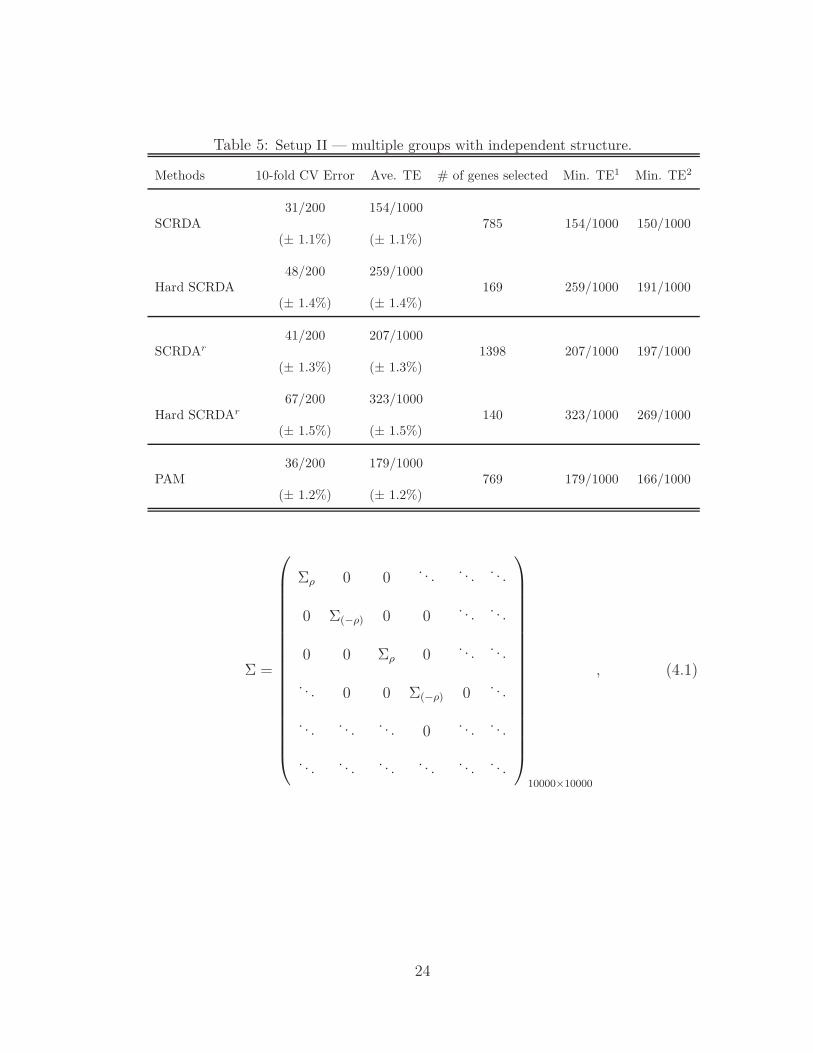
Table 5: Setup II — multiple groups with independent structure.
Methods 10-fold CV Error Ave. TE # of genes selected Min. TE1 Min. TE2
SCRDA31/200 154/1000
785 154/1000 150/1000(± 1.1%) (± 1.1%)
Hard SCRDA48/200 259/1000
169 259/1000 191/1000(± 1.4%) (± 1.4%)
SCRDAr
41/200 207/10001398 207/1000 197/1000
(± 1.3%) (± 1.3%)
Hard SCRDAr
67/200 323/1000140 323/1000 269/1000
(± 1.5%) (± 1.5%)
PAM36/200 179/1000
769 179/1000 166/1000(± 1.2%) (± 1.2%)
Σ =
Σρ 0 0. . .
. . .. . .
0 Σ(−ρ) 0 0. . .
. . .
0 0 Σρ 0. . .
. . .
. . . 0 0 Σ(−ρ) 0. . .
. . .. . .
. . . 0. . .
. . .
. . .. . .
. . .. . .
. . .. . .
10000×10000
, (4.1)
24

with each diagonal block being the following autoregressive structure:
Σρ =
1 ρ . . . ρ98 ρ99
ρ 1. . .
. . . ρ98
.... . .
. . .. . .
...
ρ98 . . .. . .
. . . ρ
ρ99 ρ98 . . . ρ 1
100×100
. (4.2)
The block size is 100 × 100 and there are totally k = 100 blocks. We assume
the autocorrelation within each block is |ρ| = 0.9 and we set alternating signs for
each block. n = 200 training samples and m = 1000 test samples are generated
with half from each class.
This simulation setup does have sound basis in real microarray data. It is
common knowledge that genes are networked together in pathways. Although it
is true that weak connections between groups may exist, independence between
groups is usually a reasonable assumption. Also, within each group, genes are
either positively or negatively correlated and due to their relative distance in
the regulatory pathway, the further apart two genes, the less correlation between
them. These are exactly the reasons why we use the above simulation model. From
the results in Table 6, we can clearly see that the SCRDA method outperforms
PAM by a significant margin. Considering this is only a two-group classification
problem mimicking the real microarray data, we should expect the difference will
25

be more significant when the number of classes is large as we have observed for
the Tamayo and Brown data.
Table 6: Setup III — two groups with dependent structure.
Methods 10-fold CV Error Ave. TE # of genes selected Min. TE1 Min. TE2
SCRDA25/200 108/1000
282 107/1000 94/1000(± 1.0%) (± 1.0%)
Hard SCRDA21/200 96/1000
167 92/1000 86/1000(± 1.0%) (± 1.0%)
SCRDAr
25/200 123/1000283 123/1000 113/1000
(± 1.0%) (± 1.0%)
Hard SCRDAr
25/200 125/1000116 125/1000 111/1000
(± 1.0%) (± 1.0%)
PAM36/200 170/1000
749 170/1000 167/1000(± 1.2%) (± 1.2%)
5 Feature Selection by the SCRDA Method
Remember that the discriminant function (2.5) is linear in X with coefficients
vector Σ̃−1x̄g. Now if the i-th element of the coefficients vector is 0 for all 1 ≤
g ≤ G, then it means gene i doesn’t contribute to our classification purpose
and hence can be eliminated. Therefore, SCRDA potentially can be used for
the gene selection purpose. For example, as shown in Table 7, the number of
genes that are truly differentially expressed is 100, 280 and 200 respectively in
26

the 3 simulation setups above. Correspondingly, the SCRDA method picks out
240, 785 and 282 genes in each setup. Among these genes, 82, 204 and 138 are
truly differentially expressed respectively. The detection rate is at least 70% in
all situations. However, the false positive rate is also high, especially when the
number of classes is large. For now, there is not a good way to adjust this high
false positive rate. Therefore, SCRDA can be conservatively used as gene selection
method.
Table 7: Feature selection by SCRDA.
Setup I Setup II Setup III
# of True Positive (T ) 100 280 200
# of Total Positive Detected (A) 240 785 282
# of True Positive Detected (M) 82 204 138
Detection Rate (d = M/T ) 82.0% 72.8% 69.0%
False Positive (q = 1 − M/A) 65.8% 74.0% 51.1%
6 Discussion
Through comparisons using both real microarray data sets and simulated data
sets, we have shown that the SCRDA method can be a promising classification
tool. Particularly, it is consistently better than its sibling method, PAM in many
problems. This new method is also very competitive to some other methods, e.g.,
support vector machines.
27
This new method is not only empirically useful in terms of classification perfor-
mance, it also has some interesting theoretical implications, which we will discuss
carefully in a future paper. For example, it can be shown that the regularized
discriminant function (2.5) is equivalent to the penalized log-likelihood method
and in some special cases, our new method SCRDA can be related to another
recently proposed new method called “elastic net” (Zou and Hastie, 2005). These
results are interesting since not only do they give different perspectives of statis-
tical methods, they also provide new computational approaches. For example, an
alternative method for estimating the shrunken regularized centroids other than
the way we have proposed in this paper is to solve the solution of the mixed L1-L2
penalty function. This has been made possible as the problem will convert to the
usual LASSO (Tibshirani, 1996) solution. And with the emergence of the new
algorithm LARS (Efron et al., 2004), efficient numerical solution is also available.
As mentioned before, choosing the optimal parameter pairs for the SCRDA
method is not as straightforward as in PAM and in some cases, the process can be
somewhat tedious. The guidelines given in Section 3.4 work generally well, at least
for all the data examples provided in this paper. However, it may require some
experience with the SCRDA method to get the best result. Also, the computation
in the SCRDA method is not as fast as in PAM due to two reasons. First, we have
two parameters (α, ∆) to optimize over a 2-dimensional grid rather than the 1-
dimensional one in PAM. Second, although the SVD algorithm is very efficient, the
28

computation still involves large matrix manipulation in practice, while only vector
operations are involved in PAM. On the other hand, as shown in this paper, PAM
doesn’t always do a worse job than the SCRDA method. In some situations, e.g.,
when the number of classes is small or the covariance structure is nearly diagonal,
PAM is both accurate in prediction and computationally efficient. Therefore, we
recommend using the SCRDA method only when PAM cannot perform well in
classification.
Also, the SCRDA method can be used directly for gene selection proposes. As
we have seen in Section 5, the selection process of SCRDA is rather conservative,
tending to include many more genes unnecessary. But overall speaking, it is not
generally worse than PAM. And since it includes most of the genes that are truly
differentially expressed, it is a safer way of including the ones we really should
detect.
29

References
Dettling, M. (2004). Bagboosting for tumor classification with gene expression
data. Bioinformatics , 20(18), 3583–3593.
Dipillo, P. (1976). The application of bias to discriminant analysis. Communica-
tion in Statistics — Theory and Methodology , A5, 843–854.
Dipillo, P. (1977). Further application of bias discriminant analysis. Communi-
cation in Statistics — Theory and Methodology , A6, 933–943.
Efron, B., Hastie, T., Johnstone, I., and Tibshirani, R. (2004). Least angle re-
gression. Annals of Statistics , 32, 407–499.
Friedman, J. (1989). Regularized discriminant analysis. Journal of American
Statistical Association, 84, 165–175.
Golub, T., Slonim, D., Tamayo, P., Huard, C., Gaasenbeek, M., Mesirov, J.,
Coller, H., Loh, M., Downing, J., and Caligiuri, M. (1999). Molecular clas-
sification of cancer: class discovery and class prediction by gene expression
monitoring. Science, 286, 531–536.
Hastie, T., Tibshirani, R., and Friedman, J. (2001). The Elements of Statistical
Learning . Springer.
Hoerl, A. and Kennard, R. (1970). Ridge regression: biased estimation for non-
orthogonal problems. Technometrics, 12, 55–67.
30

Ramaswamy, S., Tamayo, P., Rifkin, R., Mukherjee, S., Yeang, C., Angelo, M.,
Ladd, C., Reich, M., Latulippe, E., Mesirov, J., Poggio, T., Gerald, W., Loda,
M., Lander, E., and Golub, T. (2001). Multiclass cancer diagnosis using tumor
gene expression signature. PNAS , 98, 15149–15154.
Tibshirani, R. (1996). Regression shrinkage and selection via the lasso. Journal
of Royal Statistical Society, Series B , 58(1), 267–288.
Tibshirani, R., Hastie, T., Narashimhan, B., and Chu, G. (2003). Class prediction
by nearest shrunken centroids with applications to dna microarrays. Statistical
Science, 18, 104–117.
Zhu, J. and Hastie, T. (2004). Classification of gene microarrays by penalized
logistic regression. Biostatistics , 5(3), 427–443.
Zou, H. and Hastie, T. (2005). Regularization and variable selection via the elastic
net. Journal of Royal Statistical Society, Series B , 67(2), 301–320.
31