regularized estimation of main and rf field...

Regularized Estimation of Main and RF FieldInhomogeneity and Longitudinal Relaxation Rate in

Magnetic Resonance Imaging

by

Amanda K. Funai

A dissertation submitted in partial fulfillmentof the requirements for the degree of

Doctor of Philosophy(Electrical Engineering: Systems)

in The University of Michigan2011

Doctoral Committee:

Professor Jeffrey A. Fessler, ChairProfessor Thomas L. ChenevertProfessor Douglas C. NollAssociate Professor Anna C. GilbertAssistant Professor Clayton D. Scott

c© Amanda Funai 2011

All Rights Reserved

To my husband, Katsu, and my two sons, Andrew and Seth

ii

ACKNOWLEDGEMENTS

I would like to acknowledge the following people who have been instrumental in me

finishing this dissertation. First, my committee. Most especially, my advisor Jeff for his

invaluable advice and encouragement. Also, especially Doug for his indispensible knowl-

edge of MRI. I would also like to thank all the members of Jeff and Doug’s lab groups -

their comments and support throughout graduate school havebeen invaluable. I would like

to especially thank those who collected MRI data for me, WillGrissom and Jon Nielsen.

A thank you to all support staff at Rackham and EECS, especially Becky Turanski and her

support and encouragement. A very hearty thanks to all my sources of funding, including

Rackham, EECS, NSF, and NIH. And most of all, thanks to my family and friends, most

especially my husband and his unwavering support through these busy and stressful years

of graduate school.

iii

TABLE OF CONTENTS

DEDICATION . . . . . . . . . . . . . . . . . . . . . . . . . . . . . . . . . . . ii

ACKNOWLEDGEMENTS . . . . . . . . . . . . . . . . . . . . . . . . . . . . iii

LIST OF FIGURES . . . . . . . . . . . . . . . . . . . . . . . . . . . . . . . . vii

LIST OF TABLES . . . . . . . . . . . . . . . . . . . . . . . . . . . . . . . . . xii

LIST OF APPENDICES . . . . . . . . . . . . . . . . . . . . . . . . . . . . . . xiii

ABSTRACT . . . . . . . . . . . . . . . . . . . . . . . . . . . . . . . . . . . . . xiv

CHAPTER

I. Introduction . . . . . . . . . . . . . . . . . . . . . . . . . . . . . . . . . 1

1.1 Contribution of Thesis . . . . . . . . . . . . . . . . . . . . . . . . 3

II. MRI Background . . . . . . . . . . . . . . . . . . . . . . . . . . . . . . 5

2.1 Three Magnetic Fields . . . . . . . . . . . . . . . . . . . . . . . . 52.1.1 B0, the Main Field . . . . . . . . . . . . . . . . . . . . 62.1.2 Radio frequency field (B1) . . . . . . . . . . . . . . . . 72.1.3 Field Gradients . . . . . . . . . . . . . . . . . . . . . . 8

2.2 Bloch Equation . . . . . . . . . . . . . . . . . . . . . . . . . . . 82.3 Imaging . . . . . . . . . . . . . . . . . . . . . . . . . . . . . . . 9

2.3.1 Excitation . . . . . . . . . . . . . . . . . . . . . . . . . 102.3.2 Signal Equation . . . . . . . . . . . . . . . . . . . . . . 142.3.3 Gradients . . . . . . . . . . . . . . . . . . . . . . . . . 152.3.4 Multiple Transmit Coils . . . . . . . . . . . . . . . . . 162.3.5 Noise in MRI . . . . . . . . . . . . . . . . . . . . . . . 16

2.4 MRI Field Inhomogeneity . . . . . . . . . . . . . . . . . . . . . . 172.4.1 Main Field (B0) Inhomogeneity . . . . . . . . . . . . . 172.4.2 Radio Frequency field Inhomogeneity . . . . . . . . . . 19

iv

III. Iterative Estimation Background . . . . . . . . . . . . . . . . . . . . . 21

3.1 Bayesian Estimators . . . . . . . . . . . . . . . . . . . . . . . . . 223.2 ML Estimator . . . . . . . . . . . . . . . . . . . . . . . . . . . . 223.3 Penalized-Likelihood Estimators . . . . . . . . . . . . . . . . . .233.4 Cramer-Rao Bound . . . . . . . . . . . . . . . . . . . . . . . . . 243.5 Spatial Resolution Analysis . . . . . . . . . . . . . . . . . . . . . 253.6 Minimization via Iterative Methods . . . . . . . . . . . . . . . . .26

3.6.1 Optimization Transfer . . . . . . . . . . . . . . . . . . 273.6.2 Preconditioned Gradient Descent: PGD . . . . . . . . . 28

IV. Field Map B0 Estimation . . . . . . . . . . . . . . . . . . . . . . . . . . 29

4.1 Introduction . . . . . . . . . . . . . . . . . . . . . . . . . . . . . 294.2 Multiple Scan Fieldmap Estimation - Theory . . . . . . . . . . .. 30

4.2.1 Reconstructed Image Model . . . . . . . . . . . . . . . 304.2.2 Conventional Field Map Estimator . . . . . . . . . . . . 314.2.3 Other Field Map Estimators . . . . . . . . . . . . . . . 314.2.4 Multiple Scan Model . . . . . . . . . . . . . . . . . . . 334.2.5 ML Field Map Estimation . . . . . . . . . . . . . . . . 334.2.6 Special Case:L = 1 . . . . . . . . . . . . . . . . . . . 354.2.7 PL Field Map Estimation . . . . . . . . . . . . . . . . . 364.2.8 Spatial Resolution Analysis . . . . . . . . . . . . . . . 384.2.9 Qualitative Example:L = 1 . . . . . . . . . . . . . . . 414.2.10 Theoretical Improvements Over 2 Data Sets . . . . . . . 41

4.3 Experiments . . . . . . . . . . . . . . . . . . . . . . . . . . . . . 454.3.1 Simulation . . . . . . . . . . . . . . . . . . . . . . . . 454.3.2 MR Data . . . . . . . . . . . . . . . . . . . . . . . . . 544.3.3 Application to EPI Trajectories . . . . . . . . . . . . . . 564.3.4 Fieldmap estimation in k-space . . . . . . . . . . . . . 58

4.4 Discussion . . . . . . . . . . . . . . . . . . . . . . . . . . . . . . 59

V. B+1 Map Estimation . . . . . . . . . . . . . . . . . . . . . . . . . . . . . 61

5.1 Introduction . . . . . . . . . . . . . . . . . . . . . . . . . . . . . 615.2 B+

1 Map Estimation: Theory . . . . . . . . . . . . . . . . . . . . 625.2.1 ConventionalB+

1 map . . . . . . . . . . . . . . . . . . 625.2.2 Signal model for multiple coils, multiple tip angles/coil

combinations . . . . . . . . . . . . . . . . . . . . . . . 645.2.3 Regularized estimator . . . . . . . . . . . . . . . . . . 67

5.3 Experiments . . . . . . . . . . . . . . . . . . . . . . . . . . . . . 695.3.1 Simulation Study . . . . . . . . . . . . . . . . . . . . . 695.3.2 MRI Phantom Study . . . . . . . . . . . . . . . . . . . 81

5.4 Discussion . . . . . . . . . . . . . . . . . . . . . . . . . . . . . . 82

v

VI. Joint B+1 , T1 Map Estimation . . . . . . . . . . . . . . . . . . . . . . . 84

6.1 JointT1 andB+1 Estimation: Motivation . . . . . . . . . . . . . . 84

6.2 Overview of CurrentT1 Mapping Methods . . . . . . . . . . . . . 866.2.1 Look-Locker imaging sequence . . . . . . . . . . . . . 876.2.2 SSI imaging sequence . . . . . . . . . . . . . . . . . . 876.2.3 SSFP pulse sequence . . . . . . . . . . . . . . . . . . . 906.2.4 Overview of Current JointT1 andB1 Estimation . . . . 92

6.3 Limitations of Current Methods and Possible Solutions . .. . . . 956.3.1 B+

1 inhomogeneity . . . . . . . . . . . . . . . . . . . . 956.3.2 Slice profile effects, Bloch equation non-linearity,and

flip angle miscalibration . . . . . . . . . . . . . . . . . 966.3.3 Joint estimation and signal processing . . . . . . . . . . 97

6.4 Model Selection: A CRB approach . . . . . . . . . . . . . . . . . 986.4.1 General Joint Estimation Model for Model Selection . .996.4.2 Specific Joint Estimation Models for Model Selection .1016.4.3 Model Selection Method and Results . . . . . . . . . . 1026.4.4 Model Selection Discussion . . . . . . . . . . . . . . . 1046.4.5 CRB Extension: Joint estimation Versus Estimation With

Only One Unknown Variable . . . . . . . . . . . . . . . 1086.4.6 CRB Extension: Limitation of the Maximum Allowed TR1136.4.7 CRB Extension: Effect of∆B0 . . . . . . . . . . . . . 1136.4.8 CRB Extension: Possible Application to Multiple Coils .114

6.5 JointB+1 ,T1 estimation: Theory . . . . . . . . . . . . . . . . . . . 118

6.5.1 Signal model for multiple coils, multiple tip angles/coilcombinations and/or multiple TRs . . . . . . . . . . . . 118

6.5.2 Regularized estimator . . . . . . . . . . . . . . . . . . 1206.5.3 F and Slice Selection Effects . . . . . . . . . . . . . . . 123

6.6 JointB+1 ,T1 Experiments . . . . . . . . . . . . . . . . . . . . . . 125

6.6.1 Simulations . . . . . . . . . . . . . . . . . . . . . . . . 1256.6.2 Phantom Real MR Images . . . . . . . . . . . . . . . . 153

6.7 JointB+1 , T1 estimation: Discussion . . . . . . . . . . . . . . . . . 175

VII. Conclusion and Future Work . . . . . . . . . . . . . . . . . . . . . . . . 177

APPENDICES . . . . . . . . . . . . . . . . . . . . . . . . . . . . . . . . . . . 181

BIBLIOGRAPHY . . . . . . . . . . . . . . . . . . . . . . . . . . . . . . . . . 238

vi

LIST OF FIGURES

Figure

4.1 Angularly averaged FWHM of PSF. . . . . . . . . . . . . . . . . . . . . 40

4.2 Field map estimate example. . . . . . . . . . . . . . . . . . . . . . . . .42

4.3 Field map Gaussian example. . . . . . . . . . . . . . . . . . . . . . . . .45

4.4 Field map brain example. . . . . . . . . . . . . . . . . . . . . . . . . . . 46

4.5 Improvement in the RMSE for the Gaussian example by using3 data setsrather than 2 sets. . . . . . . . . . . . . . . . . . . . . . . . . . . . . . . 49

4.6 Improvement in the RMSE for the brain example by using 3 data setsrather than 2 sets. . . . . . . . . . . . . . . . . . . . . . . . . . . . . . . 50

4.7 Bias and RMSE improvement for Gaussian example. . . . . . . .. . . . 52

4.8 Bias and RMSE improvement for brain example. . . . . . . . . . .. . . 53

4.9 MR phantom data field map reconstructed using proposed method. . . . . 54

4.10 Simple field map to correct a simulated EPI trajectory. .. . . . . . . . . . 57

4.11 Grid phantom to show effects of proper field map correction. . . . . . . . 57

5.1 TrueB+1 magnitude and phase maps and object used in simulation. . . . 69

5.2 Simulated MR scans for leave-one-coil-out (LOO). . . . . .. . . . . . . 69

5.3 Figures for one coil at a time (OAAT). . . . . . . . . . . . . . . . . .. . 71

5.4 Figures for 3 coils at a time (LOO). . . . . . . . . . . . . . . . . . . .. . 72

vii

5.5 Figures for 3 coils at a time (LOO) with less measurements. . . . . . . . . 75

5.6 Figures for one coil at a time (OAAT) with less measurements. . . . . . . 76

5.7 Three of the eighteen scans taken of the phantom. . . . . . . .. . . . . . 81

5.8 Estimation of the phantom using proposed method. . . . . . .. . . . . . 82

6.1 Robustness of the SSI model at the optimal parameters. . .. . . . . . . . 105

6.2 Robustness of the AFI model at the optimal parameters. . .. . . . . . . . 105

6.3 Robustness of the BP model at the optimal parameters. . . .. . . . . . . 106

6.4 Minimum achievableσmaxb for a maximumσmax

t for two scans. . . . . . . 107

6.5 Minimum achievableσmaxb for a maximumσmax

t for eight scans. . . . . . 107

6.6 Cost of joint estimation for the SSI modelN = 2. . . . . . . . . . . . . . 108

6.7 SSI modelN = 4, compare Fig. 6.6. . . . . . . . . . . . . . . . . . . . . 109

6.8 SSI modelN = 8, compare Fig. 6.6. . . . . . . . . . . . . . . . . . . . . 109

6.9 AFI modelN = 2, compare Fig. 6.6. . . . . . . . . . . . . . . . . . . . . 110



6.12 BP modelN = 2, compare Fig. 6.6. . . . . . . . . . . . . . . . . . . . . 111

6.13 BP modelN = 4, compare Fig. 6.6. Some CRB values exceeded the axisrange. . . . . . . . . . . . . . . . . . . . . . . . . . . . . . . . . . . . . 112

6.14 BP modelN = 8, compare Fig. 6.6. . . . . . . . . . . . . . . . . . . . . 112

6.15 σb andσt as a function of upperTR limit. . . . . . . . . . . . . . . . . . . 113

6.16 Magnetic field inhomogeneity effect on SSI model. . . . . .. . . . . . . 115

6.17 Application to multiple coils for the SSI model. . . . . . .. . . . . . . . 116

6.18 Application to multiple coils for the AFI model. . . . . . .. . . . . . . . 116

viii

6.19 Application to multiple coils for the BP model. . . . . . . .. . . . . . . 117

6.20 Graph ofHR(θ,T ) for an idealized infinite sinc pulse holdingT1 constant. 126

6.21 Graph ofHR(θ,T ) for an idealized infinite sinc pulse holdingθ constant. 127

6.22 Graph ofHR(θ,T ) for an idealized infinite sinc pulse holdingT1 constant. 128

6.23 Graph of the first derivative ofHR(θ,T ) with respect toθ for an idealizedinfinite sinc pulse. . . . . . . . . . . . . . . . . . . . . . . . . . . . . . . 129

6.24 Graph of the first derivative ofHR(θ,T ) with respect toT for an idealizedinfinite sinc pulse. . . . . . . . . . . . . . . . . . . . . . . . . . . . . . . 130

6.25 Graph of the first derivative ofHR(θ,T ) with respect toT for an idealizedinfinite sinc pulse. . . . . . . . . . . . . . . . . . . . . . . . . . . . . . . 131

6.26 True simulated maps. . . . . . . . . . . . . . . . . . . . . . . . . . . . . 132

6.27 Simulated noisy images. . . . . . . . . . . . . . . . . . . . . . . . . . .134

6.28 MagnitudeB+1 maps for OAAT at 60 dB with 12 measurements. . . . . . 136

6.29 PhaseB+1 maps for OAAT at 60 dB with 12 measurements. . . . . . . . . 137

6.30 T1 maps for OAAT at 60 dB with 12 measurements. . . . . . . . . . . . . 138

6.31 f estimates for OAAT at 60 dB with 12 measurements. . . . . . . . . . .139

6.32 MagnitudeB+1 maps for LOO at 60 dB with 12 measurements. . . . . . . 140

6.33 PhaseB+1 maps for LOO at 60 dB with 12 measurements. . . . . . . . . . 141

6.34 T1 maps for LOO at 60 dB with 12 measurements. . . . . . . . . . . . . . 143

6.35 f estimates for LOO at 60 dB with 12 measurements. . . . . . . . . . . .144

6.36 MagnitudeB+1 maps for OAAT at 30 dB with 16 measurements. . . . . . 145

6.37 PhaseB+1 maps for OAAT at 30 dB with 16 measurements. . . . . . . . . 146

6.38 T1 maps for OAAT at 60 dB with 12 measurements. . . . . . . . . . . . . 147

6.39 f estimates for OAAT at 30 dB with 16 measurements. . . . . . . . . . .148

ix

6.40 MagnitudeB+1 maps for LOO at 30 dB with 12 measurements. . . . . . . 149

6.41 PhaseB+1 maps for LOO at 30 dB with 12 measurements. . . . . . . . . . 150

6.42 T1 maps for LOO at 30 dB with 12 measurements. . . . . . . . . . . . . . 151

6.43 f estimates for LOO at 30 dB with 12 measurements. . . . . . . . . . . .152

6.44 |y| transmitting individually for each of the four coils with TR= 2000 ms. 153

6.45 Initial phantom estimates. . . . . . . . . . . . . . . . . . . . . . . .. . 154

6.46 Final phantom regularized estimates. . . . . . . . . . . . . . .. . . . . . 155

6.47 Final phantom unregularized estimate. . . . . . . . . . . . . .. . . . . . 155

6.48 Phantom model fit,θ = 5 degrees, whereθ = αb . . . . . . . . . . . . . 157




6.52 Phantom model fit with respect to b1, TR = 20 ms . . . . . . . . . .. . . 161

6.53 Phantom model fit with respect to b1, TR = 60 ms . . . . . . . . . .. . . 162

6.54 Phantom model fit with respect to b1, TR = 100 ms . . . . . . . . .. . . 163

6.55 Phantom model fit with respect to b1, TR = 200 ms . . . . . . . . .. . . 164

6.56 Phantom model fit with respect to b1, TR = 2000 ms . . . . . . . .. . . 165

6.57 Phantom magnitude data with all four coils turned on at four repetitiontimes. . . . . . . . . . . . . . . . . . . . . . . . . . . . . . . . . . . . . 166

6.58 Phantom: Regularized estimates for all coils turned on. . . . . . . . . . . 167

6.59 Phantom: estimate for individual coil maps. . . . . . . . . .. . . . . . . 167

6.60 Final regularized estimates using all data for the second phantom experi-ment. . . . . . . . . . . . . . . . . . . . . . . . . . . . . . . . . . . . . 168


x






A.1 Illustration ofϕ(t) and quadratic surrogates for several values ofs. . . . 185

B.1 Graph ofHR(θ) for a Gaussian and truncated sinc pulse. . . . . . . . . . 189

B.2 Graph of the derivative ofHR(θ) for a Gaussian and truncated sinc pulse. 190

K.1 Intermediate initial maps using triple angle method. . .. . . . . . . . . . 227

K.2 Intermediate initialB+1 map when TR is varied. . . . . . . . . . . . . . . 229

xi

LIST OF TABLES

Table

4.1 Phantom NRMSE for two representative slices . . . . . . . . . .. . . . . 52

5.1 Simulation NRMSE (%) for three selected excitation pulses averagedover 20 realizations . . . . . . . . . . . . . . . . . . . . . . . . . . . . . 74

5.2 Simulation NRMSE (%) for proposed methodM = 5 versus conven-tional DAM methodM = 8 averaged over 20 realizations (truncated sincpulse with SNR=30dB) . . . . . . . . . . . . . . . . . . . . . . . . . . . 79

5.3 Simulation NRMSE (%) using the correct slice profile for estimation ver-sus using the conventional ideal pulse profile for estimation . . . . . . . . 80

6.1 Optimized scan parameters based on (6.17) . . . . . . . . . . . .. . . . 104

6.2 Optimized scan parameters based on (6.17) with smallB+1 range . . . . . 117

6.3 Masked NRMSE for simulated images for differentα, numbers of mea-surements, and SNR . . . . . . . . . . . . . . . . . . . . . . . . . . . . . 142

6.4 Changes in NRMS with a change of TR, 1 estimate, 4 coils, 16 measure-ments, 30 iterations with 10 PGD iterations, SNR = 30 dB,α = 1.38 · [1234]147

6.5 Changes in NRMS with a change ofα, only 1 total scan each, 4 coils, 16measurements, 15 iterations with 5 PGD iterations, SNR = 30 dB, TR =.68s . . . . . . . . . . . . . . . . . . . . . . . . . . . . . . . . . . . . . 151

xii

LIST OF APPENDICES

Appendix

A. B0 Minimization Algorithms . . . . . . . . . . . . . . . . . . . . . . . . . 182

B. B1: F and Slice Selection Effects . . . . . . . . . . . . . . . . . . . . . . . 187

C. B1: Derivation of cost function gradients and separable surrogates . . . . . . 191

D. B1: Derivatives ofF . . . . . . . . . . . . . . . . . . . . . . . . . . . . . . 199

E. B1: Initial estimate forf andx . . . . . . . . . . . . . . . . . . . . . . . . 205

F. B1: What if α is complex? . . . . . . . . . . . . . . . . . . . . . . . . . . 207

G. B1: Spatial Resolution Analysis . . . . . . . . . . . . . . . . . . . . . . . . 211

H. B1/T1: Derivatives of Signal Models: SSI and AFI . . . . . . . . . . . . . . 215

I. B+1 ,T1: Derivation of cost function gradients . . . . . . . . . . . . . . . . .218

J. B+1 , T1: Derivatives ofF . . . . . . . . . . . . . . . . . . . . . . . . . . . 222

K. B+1 , T1: Initial estimate forB+

1 , T1, andf . . . . . . . . . . . . . . . . . . 224

L. B+1 , T1: Spatial Resolution Analysis . . . . . . . . . . . . . . . . . . . . . 230

M. B+1 , T1: Constrained estimation forT1 . . . . . . . . . . . . . . . . . . . . 236

xiii

ABSTRACT

Regularized Estimation of Main and RF Field Inhomogeneity and LongitudinalRelaxation Rate in Magnetic Resonance Imaging

by

Amanda K. Funai

Chair: Jeffrey A. Fessler

In designing pulses and algorithms for magnetic resonance imaging, several simplifications

to the Bloch equation are used. However, as magnetic resonance (MR) imaging requires

higher temporal resolution and faster pulses are used, simplifications such as uniform main

field (B0) strength and uniform radio-frequency (RF) transmit coil field (B+1 ) strength no

longer apply. Ignoring these non-uniformities can cause significant distortions. Accurate

maps of the main and RF transmit coil field inhomogeneity are required for accurate pulse

design and imaging. Standard estimation methods yield noisy maps, particularly in image

regions having low spin density, and ignore other importantfactors, such as slice selection

effects inB1 mapping andT2 effects inB0 mapping. This thesis uses more accurate signal

models for the MR scans to derive iterative regularized estimators that show improvements

over the conventional unregularized methods through Cramer-Rao Bound analysis, simu-

lations, and real MR data.

In fast MR imaging with long readout times, field inhomogeneity causes image dis-

tortion and blurring. This thesis first describes regularized methods for estimation of the

off-resonance frequency at each voxel from two or more MR scans having different echo

xiv

times, using algorithms that decrease monotonically a regularized least-squares cost func-

tion.

A second challenge is that RF transmit coils produce non-uniform field strengths, so an

excitation pulse will produce tip angles that vary substantially over the field of view. This

thesis secondly describes a regularized method forB+1 map estimation for each coil and for

two or more tip angles. Using these scans and known slice profile, the iterative algorithm

estimates both the magnitude and phase of each coil’sB+1 map.

To circumvent the challenge in conventionalB+1 mapping sequences of an long rep-

etition time, this thesis thirdly describes a regularized method for jointB+1 andT1 map

estimation using a regularized method based on a penalized-likelihood cost function us-

ing the steady-state incoherent (SSI) imaging sequence with several scans with varying tip

angles or repetition times.

xv

CHAPTER I

Introduction

Magnetic resonance imaging (MRI) is a very important and powerful imaging modality,

being both safe and non-invasive, while still sensitive to alarge variety of tissue properties.

Careful manipulation of magnetic fields allows for imaging ofan object’s interior and its

structure, metabolism, and function. MR uses three main magnetic fields, the main field

(B0), a radio-frequency field (B1), and gradient fields. The final measured MR signal

depends greatly on the applied magnetic fields magnitude andphase. Estimation of these

fields using statistical signal processing techniques is essential to create the most accurate

images possible.

A governing assumption throughout magnetic resonance (MR)is perfectly homoge-

neous main and radio-frequency fields (B0 andB1). However, homogeneous fields are

not feasible in the real world. For example, inhomogeneity in the main field arises both

from the physical design of the magnet (although this can be improved with shimming)

and also from differences in bulk magnetic susceptibility,especially on the boundary of air

and tissues, as in the sinuses. This is especially problematic at higherB0 field strengths.

Similarly,B1 (radio-frequency or RF) inhomogeneity arises from increasing distance from

transmit coils, use of surface coils, and interaction of a subject with the RF wavelength.

Homogeneity of either the main field or RF field can not be assured due to the physical

properties of MR.

1

Homogeneity assumptions were generally appropriate underlow B0 field strengths and

short read out times. However, demand for faster, higher resolution scans and methods such

as functional magnetic resonance imaging (fMRI) require fast methods and higherB0 field

strengths. As fast imaging techniques such as echo-planar imaging (EPI) and spiral scans

gain popularity, image artifacts fromB0 field inhomogeneity are visible. These artifacts

cause signal loss and result in shifts or blurring in the finalMR images, making qualitative

and quantitative analysis difficult. These effects are exacerbated in highB0 fields. Simi-

larly, as MR main fields grow in strength, image artifacts fromB1 field inhomogeneity are

visible. At higher field strengths, the RF wavelength is shortened, and experiences further

shortening due to changes in the tissue dielectric constant, resulting in higher inhomogene-

ity at higher main field strengths. The nonuniform effect in each voxel gives a possibly

different tip angle in each voxel. This gives spatially varying signal and intensity in the

image, making both qualitative and quantitative analysis difficult. Therefore, the speed

and field strength requirements of state-of-the-art MR technology further exacerbate the

problems of inhomogeneity.

Correcting for these artifacts is possible using the appropriate field map. Given a

smooth field map ofB0 inhomogeneity, conjugate phase methods can compensate forphase

accrual at each voxel, tailored RF pulses can compensate forsignal loss, or iterative recon-

struction methods can be used to obtain corrected final MR images under the condition

of an inhomogeneousB0 field. Similarly, given a map ofB1 inhomogeneity, tailored RF

pulses, parallel transmit excitation, and dynamic adjustment of RF power can compensate

for B1 inhomogeneity. Highly accurate and reliable field map estimators are required in

these intensive imaging environments.

Previous estimators have often been based on heuristic algorithms rather than on a

statistical estimation theory. These estimators are oftenlimited in scope, dependent on a

strict measurement scheme, specific imaging parameters, orignore complicating physical

effects. Additionally, these estimators often satisfy therequirement for smooth field maps

2

through low pass filtering and smoothing of calculated field maps. New statistically based

estimators that are based on more comprehensive models are needed. Estimators are needed

that incorporate the knowledge that true field maps are smooth with an understanding of

the effect of smoothing on image spatial resolution. This thesis presents three separate

estimators that satisfy these desired estimator properties.

Chapter II first presents a short introduction to MRI. Section2.4 follows with a brief

discussion of the effects on field inhomogeneity - the motivation for new statistical es-

timators. Chapter III overviews some principles of iterative penalized estimator design,

which are used as the solution in this report. Chapter IV tackles the problem of main field

map estimation, considering both current solution and proposing the new solution as well

as demonstrating its effectiveness. Chapter V similarly looks atB1 map estimators, con-

sidering current solutions and proposing a new iterative estimator and demonstrating its

effectiveness. Chapter VI, noting the interdependence ofB1 and the longitudinal relax-

ation timeT1, considers current solutions toT1 mapping and jointB1, T1 mapping and

their limitations and proposes a new joint estimator forT1 andB1 which incorporates slice

profile effects and Bloch non-linearity. Finally, Chapter VII concludes, summarizing the

proposed solutions in this work and giving future work in thegoal of estimating parameter

maps in MRI.

1.1 Contribution of Thesis

This thesis proposes three new penalized-likelihood (PL) estimators based on compre-

hensive statistical models with regularization.

First, the field map PL estimator uses two or more scans to estimate field maps that in-

terpolate smoothly in voxels with low spin density and includes a simple weighting scheme

to partially account forR∗2 decay. A Cramer Rao Bound analysis aids in selection of echo

times. This estimate improves the conventional field map estimates, shown both in simula-

tion studies, as well as with real MR phantom data. The resulting improved reconstructed

3

images dramatically affects the final image quality.

Second, theB+1 PL estimator uses multiple scans and an arbitrary selectionof tip angles

to estimate both theB1 magnitude and relative phase of one or more coils assuming a very

long repetition time. This method accounts for slice selection effects by using the correct

slice profile in the model, improving results at higher tip angles. This method also smoothly

interpolates in regions with low spin density. The simulation results have less error that the

conventional estimate, even when using the standard two angles. Results are also shown

with MR phantom data.

Third, the jointB+1 /T1 PL estimator uses multiple scans and an arbitrary selectionof

tip angles and repetition times to estimate both theB1 magnitude and relative phase of

one or more coils. The estimator uses the steady-state incoherent (SSI) method based on

a Cramer Rao Bound analysis of variousB1/T1 joint estimation schemes and aids in se-

lection of imaging parameters. This method allows for shortened repetition times, and

thus faster scanning, than the previous regularizedB1 method. The regularizedB1 esti-

mates interpolate smoothly in low spin density areas with a user-chosen desired full-width

half-maximum (FWHM). Simulation results show lower error than those of the previous

estimator due to inclusion ofT1 effects.

The thesis contributes three new PL estimators that incorporate important physical ef-

fects and smooth in areas of low data magnitude in a controlled manner via a user-selected

β value. Cramer Rao bound analyses help select imaging parameters. The estimators aid

the field of MR parameter mapping to ultimately improve pulsedesign and imaging.

4

CHAPTER II

MRI Background

First, a brief overview of MRI, the magnetic fields used, and the basic equations which

govern MRI and their assumptions will be given.

Magnetic resonance imaging (MRI) is a medical imaging modality that uses magnetic

fields to image the body non-invasively and without ionizingradiation. Certain atoms

(those with an odd number of neutrons or protons) possess a characteristic called nuclear

spin angular momentum. Hydrogen, located throughout the human body in the form of

water, has a single proton and is the atom used in conventional MRI. We can visualize

these atoms as tiny spheres spinning around an axis, or a “spin”. The spins create a small

magnetic moment in the same direction as the angular momentum. Manipulating these

spins through interactions with magnetic fields creates thesignal measured in MRI. Many

of these signals, fit to a Cartesian grid, are then transformedvia a 2D (or 3D) Fourier

Transform to create the final image.

2.1 Three Magnetic Fields

Three magnetic fields are used in signal acquisition in MRI: 1) B0, the main field, 2)

B1, the radio frequency field, and 3) affine perturbations ofB0 called field gradients.

5

2.1.1 B0, the Main Field

Normally, the spins are in random directions, creating a netmagnetic moment of zero.

However, when a magnetic field is introduced (by convention in the z, or longitudinal,

direction), magnetic moments can only be oriented parallelor anti parallel to the field, as

explained by quantum physics. The parallel state is a lower energy state, while the anti

parallel state is a higher energy state. Thus, slightly moreatoms (only a few parts per

million) will align in the parallel state, creating a net magnetic moment (referred to as the

net magnetization) aligned parallel to the main field,B0.

These atoms also possess a second important characteristic: magnetic resonance. This

property causes the spins to precess about the z direction like a spinning top when the

magnetic fieldB0 is applied. The frequency of precession is governed by the Larmor

equation

(2.1) ω = γ ·B0,

whereγ is the gyromagnetic ratio (for hydrogen,γ/2π = 42.57 MHz/T). Based on this

equation, typical resonant frequencies are 63 MHz for a 1.5Tfield. If no excitation is

applied, the net magnetization is proportional to the spin density, the number of spins per

unit volume. We define the net magnetization as

M = Mx~i+My

~j +Mz~k.

A homogeneous main field is important in MRI so that the resonant frequency is con-

stant across the field. Shimming, using small coils or magnets, can be used to make a

more homogeneous main field. Main fields are usually in the range of a few Tesla. How-

ever, as field strengths become higher (for example, 3T and higher), making the main field

homogeneous becomes more and more difficult.

6

2.1.2 Radio frequency field (B1), Excitation and Relaxation

The second magnetic field applied is a radio frequency field, calledB1. This alternating

electromagnetic field (i.e., a radio frequency (RF) field) is applied, tuned to the Larmorfre-

quency, during the excitation phase of scanning to tip the magnetization into the transverse

plane.. This applies a torque to the net magnetization vector, causing that vector to tip. The

tip angle is governed by the strength of the RF field and the length of time it is applied.

Typically, an angle of 90 degrees is desired so that the net magnetization is in the x-y plane.

If the radio frequency field is inhomogeneous, then the net magnetization vector will

be tipped by a different angle at each location in the ROI. This can cause problems in

excitation.

After excitation, the net magnetization returns to equilibrium in the longitudinal plane.

The vector continues to precess at the Larmor frequency during relaxation. This is called

relaxation. Relaxation is governed by two constants (T1 andT2) which depend on the ob-

ject’s material.T1 is the spin-lattice constant and involves energy exchange between spins

and the surrounding electrons. The values are in the range ofhundreds of milliseconds.T1

specifies how the longitudinal magnetization recovers:

(2.2) Mz(t) = M0(1 − e−t/T1),

whereM0 is the equilibrium nuclear magnetization.T2 is the spin-spin time constant and

involves interactions between the spins.T2 is normally in the tens of milliseconds.T2

specifies how the magnitude of the transverse magnetization(in the XY plane) decays:

(2.3) Mxy(t) = M0 e−t/T2 ,

whereMxy = Mx + iMy. T1 andT2 do not affect the precession of the net magnetization

vector, but do affect its length. Interestingly, the net magnetization vector can change length

7

and differ from its equilibrium value during relaxation depending on the values ofT1 and

T2. In fact, magnetization can even disappear for a time and then return.

The magnetization vector precesses at the Larmor frequencywhile returning to equi-

librium. This precession, by Faraday’s Law, causes an electromagnetic force in a RF coil

that is measured. This signal is the MRI signal. This signal,therefore, depends not only on

spin density, but also onT1 andT2.

2.1.3 Field Gradients

To create an image, there needs to be spatially dependent information. The addition

of field gradients which, encode this information earned itsinventor, Paul C Lauterbur and

Peter Mansfield, a Nobel Prize in 2003. Linear field gradientsare applied to the main field.

The field perturbation is the same in the direction asB0, but its magnitude varies at spatial

coordinates. A general gradient can be expressed as

(2.4) G = Gx~i+Gy

~j +Gz~k,

where~i,~j, and~k are unit vectors. The main field can then be expressed as

~B(r) = (B0 +Gxx+Gyy +Gzz)~k = (B0 + G · ~r)~k.

By varying these field gradients, many signals can be collected and then arranged on a

Cartesian grid. Then, a simple 2D Fourier transform of the collected signal gives the final

image.

2.2 Bloch Equation

The behavior of the magnetization vector is governed by a phenomenological equation

called the Bloch equation. This equation describes the precession and relaxation effects in

8

the previous section. The Bloch equation is given below:

(2.5)dM

dt= M × γB − Mx

~i+My~j

T2

− (Mz −Mo)~k

T1

.

The first term describes precession and influences the direction of the net magnetization.

For example, the change in magnetization is proportional tothe cross product ofM and

B. If B remains constant (i.e., our main field), then the angle betweenM andB will

not change and we will have precession as specified by the Larmor equation. The second

term describes the relaxation controlled by the relaxationratesT1 andT2 and influences the

length of the net magnetization.

There is no known general solution to the Bloch equation; however, when certain sim-

plifications are made, the differential equation can be solved. One important example is

whenRF = 0, which applies during relaxation when the RF is not applied.Using the

expression for a general gradient (2.4), the transverse (X-Y plane) component of the Bloch

equation isdMxy

dt= −

(1

T2(~r)+ i(ω0 + ω(~r, t))

)Mxy.

This simple differential equation thus has the solution

(2.6) Mxy(~r, t) = M0(~r) e−t/T2(~r) e−ıω0t e−ıγG·~rt .

2.3 Imaging

Creating an MR image requires two basic steps. Excitation consists of using a RF pulse

to excite the volume (or a portion thereof). Then, gradientsare used to spatially encode

the information. Finally, during readout, the transverse component of the magnetization

signal is read. Usually, this process is repeated several times by waiting until equilibrium

is reached between excitations. The collection of recordedsignals are rearranged into a 2D

array and then the Fourier transform yields a two-dimensional image.

9

2.3.1 Excitation

Excitation involves using an RF pulse to “excite” spins, or tip spins by some angle.

Non-selective excitation excites the entire volume, whileselective excitation excites just a

slice of the volume. Excitation is based on the principles discussed in Section 2.1.2.

2.3.1.1 Non-selective Excitation

In non-selective excitation, all the spins in the entire volume are excited by the RF

pulse, causing them to tip by an angle determined by the duration and power of the pulse.

To analytically solve the Bloch equation in this situation,one uses a few simplifications.

First, no gradients are applied - the only operating magnetic fields are the RF pulse (theB1

field) and the main field,B0. Relaxation is ignored because the typical length of an RF

pulse is very short (less than 1 millisecond).

Two RF coils are used in MR: one coil, the transmit coil, creates the RF field that excites

the spins; the second coil, the receive coil receives the RF signal from the precessing spins.

Sometimes, one coil will be used for both of these two purposes or multiple coils will be

used for either the transmit coil or the receive coil or both.While ideally each of these coils

would have a uniform response (e.g., for the receive coil, two identical precessing spins

in different locations would generate the same emf), real RFcoils have a coil response

function that varies as a function of space,B+1 (~r) (response of the transmit coil(s)) and

Breceive(~r) (response of the receive coil(s)), where~r is the space variable. (Note - if more

than one coil is used for transmitting or receiving, each will have its own unique response.)

The inhomogeneity of the coil response can be very problematic. A non-uniform receive

coil response creates intensity differences - those areas with a smallerBreceive will appear

darker compared to areas with a larger value ofBreceive. This can make MR images more

difficult to interpret. A non-uniform transmit coil response, however, is much more prob-

lematic because it leads directly to varying flip angle and influences the signal equation in

a more complicated way. Non-uniform flip angles, orB1 field inhomogeneity, is explained

10

further in Section 2.4.

When an amplitude-modulated signal is injected into either coil, the coil induces a

magnetic field calledBlin1 (~r, t):

(2.7) Blin1 (~r, t) = a1(t) cos(ωt+ φ1(t) +φ′

k)B+1 (~r),

wherea1(t) andφ1(t) are the input amplitude and phase to the coil andφ′k is the modulator

phase offset. We assume here thatBlin1 is exactly on-resonance andω is the Larmor fre-

quency. The transverse component of this field, or the part ofthe field that is perpendicular

toB0, influences spins. We can break this field into two circularlypolarized fields, a right

and a left-handed field; because the left-handed field rotates in the same direction as the

rotating spins, this field is more resonant with the spins andthe right-handed field has only

a negligible effect on the spins (and is thus ignored) [92].B1 is the left-handed circularly

polarized field and is expressed as:

(2.8) B1(~r, t) = B+1 (~r)a1(t)[cos(ωt+ φ1(t) +φ′

k)~i− sin(ωt+ φ1(t) +φ′

k)~j].

This field is referred to as theB+1 field and is the active field during transmission (in this

thesis, we are referring to this circularly polarized field when we are estimating theB1 field

and inhomogeneity in Chapter V and Chapter VI).

BecauseB1 is precessing, changing our unit directional vectors to vectors that are ro-

tating clockwise at an angular frequencyω can greatly simplify description of these fields.

This is called a rotating frame. We can choose a rotating frame that is precessing at the

Larmor frequency or at the RF frequency. Here, we assume on-resonance (i.e., the Larmor

frequency is exactly the same as that ofB1) and then these rotating frames are identical.

11

Then, the new directional vectors are defined as

~i′ , cos(ωt)~i− sin(ωt)~j

~j′ , sin(ωt)~i+ cos(ωt)~j

~k′ , ~k,

and the rotation matrixRx is given by

Rz(θ) =

cos(θ) sin(θ) 0

− sin(θ) cos(θ) 0

0 0 1

,

and the magnetization vector in the rotating frame is given by

Mrot =

[Mx′ My′ Mz′

]T

.

Then,

(2.9) Mrot(~r, t) = Rz(θ(~r))Mrot(~r, 0),

where the tip angle is defined as

(2.10) θ(~r) =

∫ t

0

ω1(~r, s)ds,

whereω1(~r, t) = γB+1 (~r)b1(t) andb1(t) , a1(t) e−iφ1(t) and the oscillator offset has been

absorbed by theB+1 .

In the rotating frame, the RF field rotates the magnetizationvector from the longitudi-

nal. The magnetization vector thus precesses along this path as it is tipped.

In the case of multiple transmit coils driven by the same RF signalb1(t) with individual

12

coil pattersB+1 k and different relative amplitudesαk, the complex coil patterns add linearly.

Although theB1 fields add linearly, the magnetization fields do not.

2.3.1.2 Selective Excitation

In selective excitation, a static z gradientGzz is applied during the RF pulse to select

only spins in a desired “slice”. Only spins where the resonant frequency matches the fre-

quency ofB1 will be excited. Again, we assumeT1 andT2 effects are negligible due to the

short pulse duration. A circularly polarized RF pulse is applied at a frequency close to the

Larmor frequency. Even with these simplifications, the Bloch equation can only be easily

solved by making the small tip-angle approximation [98]. This approximation assumes

that the system is initially at equilibrium (i.e., the magnetization vector is completely in the

longitudinal plane) and that the tip angle is small (less than 30 degrees). Under the small

tip angle assumption, we can assume thatMz ≅ M0 anddMz/dt ≅ 0. After solving the de-

coupled differential equation, the expression for the transverse component after excitation

is equal to the Fourier Transform ofB1. This relationship is [92]:

(2.11) M(t, ~r) = iM0(~r)B+1 (~r) e−ıω(z)t

∫ t

0

eıω(z)s ω1(s)ds,

whereω(z) = γGzz from which follows:

(2.12) |M(τ, z)| = M0(~r)B+1 (~r)F1Dγb1(t+ τ/2)|f=−(γ/2π)Gzz.

If we have exact resonance (i.e., eitherz = 0 orGz = 0), then the same solution applies as

in non-selective excitation - the tip angle is equal to the integral of the RF pulse. This can

be expanded to include multiple coils, as well.

Because of the Fourier Transform relationship, finding the ideal RF pulse is difficult

because both the RF pulse itself and the resultant slice profile are necessarily time limited.

An infinite sinc pulse is impossible to create in practice, asis the ideal rectangular slice

13

profile. In practice, truncated sincs or Gaussian pulses areused. This can create problems

when an algorithm is based upon the ideal of an infinitely thinand/or rectangular achieved

slice profile.

2.3.2 Signal Equation

After a portion of the volume has been excited, we must further understand the MR

signal and how to create the appropriate gradients to obtaina spatially encoded signal for

the final image.

Ideally, receiver coil(s) detect flux changes in transversemagnetization uniformly over

the entire volume or ROI. (To combat this non-ideality, manymodels add the sensitivity

pattern of the coils as a parameter [69, 113].) Each excited spin contributes to the signal.

Therefore, the signal equation is equal to the volume integral of the transverse magnetiza-

tion:

(2.13) Sr(t) =

∫

vol

Breceive(~r)M(~r, t)d~r.

We note here that this signal equation ignores constant factors and phase factors based on

ignoring T2 decay. We will also include the coil sensitivities in this analysis. In the case

where these are not appropriate assumptions, even this firstsignal equation might be called

into question. Using (2.6), the signal equation is:

(2.14) s~r(t) =

∫ ∫ ∫M0(~r)B

receive(~r) e−t/T2(~r) e−ıω0t e−ıγR t

0~G(τ)·~rdτ dxdydz.

Again, we ignore the relaxation term. We look only at the envelope of this signal and

assume no z gradient is applied. This yields the following equation:

(2.15) s(t) =

∫

x

∫

y

m(x, y)Breceive(x, y) e−ıγR t

0~G(τ)·~rdτ dxdy,

14

wherem(x, y) is the integral of the magnetization over the slice. It can bealso written

using the kspace notation (which will be explained in the next section) as:

(2.16) s(t) =

∫

x

∫

y

m(x, y)Breceive(x, y) e−ı2π(kx(t)x+ky(t)y) dxdy,

where

kx(t) = γ/2π

∫ t

0

Gx(τ)dτ(2.17)

ky(t) = γ/2π

∫ t

0

Gy(τ)dτ,(2.18)

whereGx andGy are the x and y gradients. This signal is detected by the receivers and via

a Fourier Transform (also explained in the next section) to create our MR imagem(x, y).

2.3.3 Gradients

After excitation, gradients in the x and y direction are applied to spatially encode in-

formation into the MRI signal as shown in the previous equation. This equation clearly

shows a Fourier relationship between the signal and the magnetization at kx and ky loca-

tions. These spatial frequency locations are usually referred to as kspace, where k is usually

measured in cycles/cm. Thus, each time in the signal corresponds to a Fourier transform of

kspace. This perspective greatly aids in designing trajectories.

As the gradients are applied, the spins are also simultaneously returning to equilibrium.

This free-induction decay (FID) signal is “read-out” or measured by the coils. A sufficient

amount of time (called TR or repetition time) is waited untilthe system returns to equi-

librium and then another excitation cycle begins, different gradients are applied, and the

signal is again read out.

The signal is typically largest at the center of kspace. The signal is read out here at

what is referred to as the echo time. This type of echo is called a gradient echo and is the

15

type of echo used in this thesis.

2.3.4 Multiple Transmit Coils (parallel excitation)

The severe problem ofB+1 inhomogeneity in high fields (≥ 3T ) precipitated the de-

velopment of multiple transmit coils and parallel excitation [67, 108, 134, 135, 142, 143,

145, 148]. Ideally, each coil can be adjusted with phase and amplitude to try to compen-

sate for the effects ofB1 field inhomogeneity. This led to the development of completely

separate pulses for each coil. The trend toward using highermain field strengths with their

subsequent benefits would be undermined without a strategy to compensate forB1 inho-

mogeneity. Multiple transmit coils also have other possible benefits. RF pulses could be

shortened in length or a larger space could be covered. A third possibility is decreasing

the RF power required. Parallel excitation motivates the need for accurate and efficientB+1

maps.

2.3.5 Noise in MRI

Noise in the MR signal is additive Gaussian noise [83]. The noise is primarily thermal,

the resistance coming both from the coil and body being imaged. Some noise is also pro-

duced by the pre-amplifier. However, through proper design of the coil and MR system,

the major noise source is the imaging object. Because the DFTis a unitary transform, the

final MRI also has Gaussian noise. When the kspace samples are uniform on a Cartesian

grid, the Gaussian noise is white; other sampling methods produce colored noise. Because

of complex components after the Fourier transform is taken,one usually look at the mag-

nitude of the image. This will give a Rayleigh distribution in background regions of the

image and a Rician distribution in the signal. Because the mean is usually much greater

than the variance, these distributions can be approximatedas Gaussian.

The signal to noise ratio (SNR) is affected by many factors inMRI. A general rule of

thumb is that the SNR is proportional to theB0 field strength if, as is common, the imaging

16

object is the main source of resistance. However, this relationship is quite complex because

other parameters in MR are also a function ofB0’s magnitude. SNR is proportional to the

square root of the total measurement time, whether by increasing the number of samples,

the number of signal averages, or the length of the readout time. As a rule of thumb,

increasing the spatial resolution by a factor reduces the SNR by that same factor.

2.4 MRI Field Inhomogeneity

In solving the Bloch equation as shown in Chapter II, field homogeneity is often as-

sumed. However, due to the nature of objects being imaged as well as the difficulty in

engineering perfect magnetic coils, fields are inhomogeneous. The sources of this inhomo-

geneity, its effects, and correction methods are explored in this section. As will be seen,

these correction methods require a map of the inhomogeneousfield. The estimation of

these fields is the subject of this thesis.

2.4.1 Main Field (B0) Inhomogeneity

As was seen in the Larmor equation (2.1), resonance frequency is directly related to

the magnetic field strength. Thus, main field inhomogeneity causes different resonant fre-

quencies at each spatial location. An inhomogeneous main magnet can be made more

homogeneous via shimming. However, inhomogeneity can alsoarise from the specific

morphology of the brain. Differences in the bulk magnetic susceptibility (BMS) of struc-

tures in the body cause macroscopic field inhomogeneity. Thedifference in BMS is highest

in areas where air and tissue meet; for example, in the sinuses and ear canal, lungs, and

the abdomen. There is an increased sensitivity to these problems at highB0 field strengths.

Inhomogeneity can also arise from chemical shift. Outer electrons shield the nucleus and

slightly reduce the magnetic field experienced by the nucleus. This causes a small change

in the resonant frequency as well. This chemical shift is experienced by fat and causes the

fatty parts of an image to be shifted or blurred depending on the trajectory. Because the

17

specific focus of this thesis is fMRI and fat suppression pulses are usually used, this cause

of inhomogeneity is considered negligible and not further considered in this thesis.

2.4.1.1 Effects of Inhomogeneity

Depending on the trajectory, inhomogeneity causes different effects. The need for

speed, especially in fMRI, requires use of trajectories which traverse most, if not all, of

kspace in one shot, or excitation cycle. Unfortunately, these trajectories with especially

long read out times exacerbate the problem of inhomogeneity.

Inhomogeneity affects the amplitude of the signal and causes signal loss [117]. Under

field inhomogeneity, the object has a distribution of different resonant frequencies which

gives the spins phase incoherence. When the contribution from each spin is added together,

this dephasing causes a signal loss. This effect is referredto asT ∗2 decay and causes a

much faster decay in the transverse magnetization. (Sometimes, the reciprocal ofT ∗2 orR∗

2

is used, such as in Section 4.2.4). With longer readout times, this problem becomes even

more severe and results in signal loss. If theT ∗2 decay is severe, the signal is weighted in

k-space, creating blur in the final image.

Geometric distortions can also result. In trajectories, such as echo-planar, the resulting

geometric distortion due to field inhomogeneity is a shift. However, spiral trajectories cause

a blur in the resulting image which is harder to correct for inthe image domain [66], though

both trajectories can be corrected in the signal domain.

2.4.1.2 Correction methods

Given a field map of the inhomogeneity, these effects can be corrected for. One major

correction method is conjugate phase methods, which attempt to compensate for the phase

at each voxel (e.g., [94]). These methods require a spatially smooth field map and do

not perform well where this assumption breaks down. Iterative reconstruction techniques

have also been developed, both for specific trajectories [52] and for more general situations

18

[114].

Field maps are also used in other MR applications. For example, in developing tailored

RF pulses to compensate for signal loss due to inhomogeneity, an accurate fieldmap is

required [140]. Because of the importance of accurate field map estimation for fMRI, we

focus on this problem in Chapter IV.

2.4.2 Radio Frequency field Inhomogeneity

Inhomogeneity in the RF field,B1, can be caused by many factors. HighB0 field

strengths make the RF wavelength shorter. In addition, the tissue dielectric constant causes

the RF wavelength to be even shorter. A shorter wavelength causes the RF field to interact

with the subject even more, causing even more inhomogeneity. The distance from the

transmit coil also can effect inhomogeneity. Inhomogeneity can be quite large at high

fields; at 3T, inhomogeneity ranging from 30-50% has been found [20]. Surface coils only

compound the problem and create even greater variation.

2.4.2.1 Effects ofB+1 inhomogeneity

Inhomogeneity of the RF field (B+1 ) causes a nonuniform effect on spins; the net mag-

netization vector will be tipped at different angles depending on the particular value ofB+1 .

This can make MR images very difficult to interpret due to spatially varying signal and

intensity in the image. This can be seen as lighter and darkerregions at higherB0 lev-

els (≥ 3T). In addition, the spin density will be measured incorrectly causing quantitative

problems, for example in measuring brain volumes [145].

2.4.2.2 Correction Methods

There are several methods used to try to minimizeB+1 inhomogeneity. These include

coil design and special pulses, such as adiabatic, impulse 2D pulses, 3D MDEFT imag-

ing and FLASH imaging [102]. However, correcting forB+1 inhomogeneity may still be

19

needed after minimization strategies are used or in the casewhen these trajectories are not

applicable. More recently, tailored RF pulses such as [102]have been proposed to reduce

inhomogeneity; they require use of aB+1 map. A new method in parallel transmit exci-

tation has been proposed using the transmit SENSE slice-select pulses [145] which also

requires uses of such a map. Dynamically adjusting the RF power is another option which

also requires use of aB1 map. To apply these new methods that more comprehensively

compensate forB1 inhomogeneity, an accurateB+1 map (and one that additionally includes

the phase) is required. We focus on this problem in Chapter V and Chapter VI.

20

CHAPTER III

Iterative Estimation Background

Creating a field map for eitherB0 orB+1 requires an accurate, reliable estimator based

on available measurements. Many common estimators are based on heuristic schemes

and not on a statistical model. Other common estimators disregard signal noise and its

properties. The solution of this dissertation uses statistical estimators to solve the field map

problems. Therefore, we review various statistical estimators.

The first step in estimation requires creating a model for thedata including the desired

parameter and other unknown parameters and their statistics. Next, we use this model to

create an estimator. Our goal is to estimate the field map fromthe MR data available (for

example, from an initial scan, either for the machine or for each patient). The data is usually

referred to as a vectorx, while the desired parameters (the field map) areθ. Based on a

model, there are many choices for an estimator. Each estimator is based on a different cost

function, a function which describes the cost of any particular estimate; for example, the

cost might be the mean squared error or the cost may penalize rough images. Based on the

given cost function, different estimators give different results.

One way to measure the effectiveness of an estimator is to look at its bias and variance.

The bias of an estimator is the difference between the expected value of the parameter and

the value of the parameter. Often, we desire an unbiased parameter,i.e., the bias of the

estimator is zero for each possible parameter. Ideally, we would also seek the estimator

21

with the lowest variance. However, the mean squared error isequal to the variance plus the

bias squared. Reducing the bias will increase the variance.Understanding this trade off is

important in selecting a good estimator.

3.1 Bayesian Estimators

Bayesian estimators require more data than just the parameters and the available data.

They also require a statistical distribution for the parameters called a prior distribution,

f(θ). Unfortunately in imaging problems, this distribution is usually not known; when it

can be obtained, it is often at great cost and time. These estimators minimize the average

cost:

(3.1) E [c] =

∫

Θ

∫

X

c(θ, θ)f(x|θ)f(θ)dxdθ,

wherec is the cost of an estimate based on the true value ofθ. Different cost functions

generate different estimators. A minimum mean squared error cost function yields the con-

ditional mean estimator (CME). A minimum mean absolute errorcost function yields the

conditional median estimator (CmE). A minimum mean uniform error cost function yields

the maximum a posterior estimator (MAP). One disadvantage of using these estimators is

finding an appropriate prior.

3.2 ML Estimator

The Maximum Likelihood (ML) estimator is one of the most common statistical esti-

mators in practice. This estimator maximizes the likelihood functionf(x|θ) - the density

function of the data given the parameter orf(x; θ) if θ is not random. It seeks the estimate

which best matches the data based on the likelihood function. Maximizing this function

can sometimes be difficult, but maximizing any monotone increasing function of the like-

22

lihood (for example, the log of the likelihood) also maximizes the likelihood. We usually

express the estimator as:

(3.2) θ = arg maxθ∈Θ

ln f(x|θ).

The ML estimator has many desirable properties; it is asymptotically unbiased and Gaus-

sian and is also transform invariant.

Although ML estimators are theoretically appealing, in practice, the estimators do not

always have good performance. They are often sensitive to noise or are computationally

expensive, for example, calculating the inverse of a large matrix. The performance declines

significantly as the number of parameters approaches the number of values to be estimated.

3.3 Penalized-Likelihood Estimators

There are two major options to improve the results of an ML estimator. First, we

can add more information (the prior distribution), which gives us Bayesian estimators.

However, priors are difficult to find and usually do not reflectan “average” image. A second

option is using penalized-likelihood (PL) estimators. These can be thought of as a Bayesian

(MAP) estimator with a possibly improper prior. A penalized-likelihood estimator seeks

an estimator which most closely matches the data (through the ML estimate) while also

satisfying other criteria through a penalty. The expression is shown below:

θ = arg minθ∈Θ

− ln f(x|θ) + βR(θ)(3.3)

θ = arg minθ∈Θ

Ψ(θ),(3.4)

whereΨ is the new cost function.R(θ) mapsθ to a penalty based on some characteristic -

usually data smoothness. Whenβ is large, the resulting image will be very smooth, whereas

whenβ is small, the estimate will be based more on the data and the image may be rough.

23

The user can choose this parameter independently. The most common roughness penalty

in 1D is a quadratic penalty on the difference between neighboring pixels:

(3.5) R(~y) =N∑

n=2

(yn − yn−1)2,

whereN is the number of pixels in an image. Quadratic penalties havebetter noise perfor-

mance than an ML estimator, but blur the image. This is the fundamental noise-resolution

trade off. With a PL estimator, the resolution can be quantified based on the choice ofβ,

giving the user more control on where they operate on this continuum. A multi-dimensional

quadratic penalty is similar to (3.5) but considers neighbors in each direction. Diagonal

neighbors could be given less weight than horizontal or vertical neighbors. Non-quadratic

estimators can be used to reduce noise and still not blur edges, but are more complicated

to analyze. One common roughness penalty used in the literature is the total variation

(TV) penalty, or an absolute value penaltye.g., [7]. They are useful, but suffer from the

disadvantage of not being differentiable.

3.4 Cramer-Rao Bound

The Cramer-Rao Bound (CRB) can be used on a statistical model to measure lower

bounds for any unbiased estimator. The CRB shows a region of variance that can not be

achieved by any unbiased estimator. While it is not specific toany particular estimator, we

can better understand how good our estimator is in relation to the CRB. The matrix CRB is

defined by:

Covθ

θ≥ F

−1(θ)

where

F(θ) = −E[∇2

θ ln p(Y ; θ)]

24

is the Fisher information. For an unbiased estimator, this CRB gives a scalar bound for

each estimator of each parameter (the values along the diagonal of the matrix), as well as

showing bounds for the covariance between parameters. The Fisher information measures

the average curvature of the log likelihood function by the true value of the parameter.

The CRB is applicable for an unbiased ML estimator. However, the regularization

term in a PL estimator makes the estimator inherently biasedand the CRB does not apply.

A PL estimator can operate below the curve specified by the CRB because of its bias.

Nevertheless, the CRB can give useful analysis for pixels where the SNR is high. For

pixels where the SNR is low, on the other hand, the regularizer basically just interpolates

those pixels and we are less interested in the noise properties.

PL estimators are complicated because they are defined implicitly in terms of the min-

imum of a cost function. This makes their mean and variance characteristics very difficult

to analyze carefully. Some methods have been developed in these situations, but they deal

with asymptotic relationships of the mean squared error. This has the characteristic that

mean and variance are equally weighted, whereas in applications, the relative importance

of mean and variance may differ. Some approximations do exist which look at moments,

but they are not explored further in this report.

3.5 Spatial Resolution Analysis

As explained in Section 3.3, regularizing PL estimators create blur. To chooseβ, it is

necessary to understand the spatial resolution propertiesof the estimator. Another reason

to look at the spatial resolution is to try to achieve more uniform resolution by modifying

the estimator itself. Here, by spatial resolution, we referto the impulse response of the

estimator. Although there are several ways to define the impulse response, all versions rely

on the gradient of the estimator itself. Estimators which are defined implicitly (e.g., PL

estimators) are more complicated to analyze. We would like to know the impulse response

of the estimator. Although several definitions of the impulse response are possible, the

25

general form is similar. The impulse response is the gradient of the estimator (based on

either the data or the mean data) times the gradient of the average data. Regardless of the

definition chosen, we need an expression for the gradient of the estimator. We require a few

set of conditions to find the gradient - the cost function musthave a unique minimizer, be

differentiable, and have an invertible Hessian (among other conditions). Then, the gradient

is defined. PL estimators consist of a log-likelihood terml(θ, x) and a regularization term

R(θ) as follows:

Ψ(θ, x) = l(θ, x) +R(θ).

The gradient of this estimator is then defined as (after much simplification) [30]:

(3.6) ∇θ(x) = [∇[2,0]l(θ, x) + ∇2R(θ)]−1[−∇[1,1]l(θ, x)]|θ=θ(x),

where∇[2,0] is the derivative taken twice with regard to the first argument (hereθ) and

where∇[1,1] is the derivative taken once with regard to each argument.

In this report, spatial resolution analysis was performed as in [119] and [30] using a

Taylor’s series approximation and Parseval’s relation andthen minimizing the cost function

by taking the gradient, setting it to zero, and solving. Thisis basically the same method as

described above.

3.6 Minimization of Cost Function via Iterative Methods

After defining our model and choosing an estimator, we need toactually evaluate it.

For the methods shown in this section, estimators are the extrema of a cost function. For

some problems, an analytic formula for the extrema exits. However, for most cost func-

tions, especially PL estimators which include a regularizer, this is not possible. Even for

problems where an analytic solution exists, the solution isoften not feasible numerically

(e.g., inverting a large matrix). Therefore, iterative methods which converge to a local min-

26

ima (or maxima) must be used. This is a large mathematical andstatistical topic with many

algorithms to choose from. Mathematical packages such as Matlab often contain several

built-in optimizers, such as Newton’s method or the conjugate gradient method. For the

joint B+1 , T1 estimation in Chapter VI, we used one general purpose optimization method:

preconditioned gradient descent (PGD), which is explainedin Section 3.6.2. For the first

two estimation problems in Chapter IV and Chapter V, these general purpose optimizers are

not used, because we were able to develop monotonic optimizers based on the principles

of optimization transfer. Optimization transfer is explained in Section 3.6.1. General pur-

pose optimizers often converge faster than algorithms produced from optimization transfer,

but for problems such as non-quadratic and non-convex problems, these optimizers are not

always monotonic and guaranteed to converge.

3.6.1 Optimization Transfer

Optimization transfer consists of two major principles. First, we choose a surrogate

function φ(n). This function is normally a function with an analytical minimizer or one

that is easy to find. Second, we minimize the surrogate. This minimum is not usually the

global minimum, so we must repeat these steps until the algorithm converges. The key

lies in choosing appropriate surrogate functions. They areusually designed so that: 1)

The surrogate and the cost function have the same value at each iterative step, and 2) the

surrogate function lies above the cost function. When both functions are differentiable, this

implies that the tangents are also matched at each iterativestep.

In this report, we use quadratic surrogates based on Huber’salgorithm [60, p.184-5].

These have the benefit of having an analytic solution for the minimizer of the surrogate.

For a quadratic surrogate, the following iteration will monotonically decrease the original

cost function:

(3.7) θ(n+1) = θ(n) − [∇2φ(n)]−1∇Φ(θ(n).

27

However, unlessφ(n) is separable, this inverse is not computationally practical. Therefore,

in this report, we use separable quadratic surrogates (SQS). This is explained in more detail

in Appendix A applied specifically to theB0 field map problem and in Appendix C applied

specifically to theB1 field map problem.

3.6.2 Preconditioned Gradient Descent: PGD

Gradient descent, or steepest descent, algorithms are a general optimization method

where each iteration descends a step along the negative of the gradient of the cost function.

In preconditioned gradient descent, the gradient of the cost function is first multiplied by a

preconditioning matrixP and then descended a step sizeα along that direction,

θ(n+1) = θ(n) − αP∇Ψ(θ(n)).(3.8)

A preconditioner can give much faster convergence. Under certain conditions of the gra-

dient and also the preconditioner (for example, the gradient satisfies a Lipschitz condition,

true with a twice differentiable bounded cost function, andthe preconditioner is a symmet-

ric positive definite matrix), the algorithm can be shown to monotonically decrease the cost

function. We can ensure descent and force monotonicity by reducing the step sizeα by half

until the cost function decreases. This guarantees descent, but can come a costly number

of evaluations of the cost function. This half-stepping method, as well asα selection is

explained further in Section 6.5.2.

28

CHAPTER IV

Field Map B0 Estimation

4.1 Introduction

MR 1 imaging techniques with long readout times, such as echo-planar imaging (EPI)

and spiral scans, suffer from the effects of field inhomogeneity that cause blur and im-

age distortion. To reduce these effects via field-correctedMR image reconstruction,e.g.,

[93, 107, 114, 118], one must have available an accurate estimate of the field map. A com-

mon approach to measuring field maps is to acquire two scans with different echo times,

and then to reconstruct the images (without field correction) from those two scans. The

conventional method is then to compute their phase difference and divide by the echo time

difference1. This model makes no account for noise and creates field maps that are

very noisy in voxels with low spin density. Section 4.2 first introduces this model and

then reviews standard approaches for this problem. A limitation of the standard two-scan

approach to field mapping is that selecting the echo-time-difference1 involves a trade

off: if 1 is too large, then undesirable phase wrapping will occur, but if 1 is too small,

the variance of the field map is large. One way to reduce the variance while also avoiding

phase unwrapping procedures is to acquire more than two scans,e.g., one pair with a small

echo time difference and a third scan with a larger echo time difference. By using multiple

echo readouts, the scan times may remain reasonable, at least for the modest spatial reso-

1This section is based on [44]

29

lutions needed in fMRI. Therefore, we present a general model that accommodates more

than two scans and describe a regularized least-squares field map estimation method using

those scans. Section 4.3 shows the improvements both in the estimated field maps and the

reconstructed images using multiple scans. This is shown first with simulated results in

Section 4.3.1 and then using real MR data in Section 4.3.2.

4.2 Multiple Scan Fieldmap Estimation - Theory

4.2.1 Reconstructed Image Model

The usual approach to measuring field maps in MRI is to acquiretwo scans of the object

with slightly different echo times, and then to reconstructimagesy0 andy1 (without field

correction) from those two scans,e.g., [21, 65, 87]. We assume the following model for

those undistorted reconstructed images is

y0j = fj + ǫ0j

y1j = fj eıωj1 + ǫ1j ,(4.1)

where1 denotes the echo-time difference,fj denotes the underlying complex transverse

magnetization in thejth voxel which is a function of the spin density, andεj denotes

(complex) noise. The goal in field mapping is to estimate an (undistorted) field map,

ω = (ω1, . . . , ωN), from y0 andy1, whereasf = (f1, . . . , fN) is a nuisance parameter

vector. This section reviews the standard approach for thisproblem, other approaches in

the literature, and then describes a new and improved method.

30

4.2.2 Conventional Field Map Estimator

Based on (4.1), the usual field map estimatorωj uses the phase difference of the two

images, computed as follows [47,107]:

(4.2) ωj = ∠(y0j∗y1

j )/1 .

This expression is a method-of-moments approach that wouldwork perfectly in the absence

of noise and phase wrapping, within voxels where|fj| > 0. However, (4.2) can be very

sensitive to noise in voxels where the image magnitude|fj| is small relative to the noise

deviations. Furthermore, that estimate ignores oura priori knowledge that field maps tend

to be smooth or piecewise smooth. Although one could try to smooth the above estimate

using a low pass filter, usually many of theωj values are severely corrupted so smoothing

would further propagate such errors (see Fig. 4.2 top right). Instead, we propose below to

integrate the smoothing into the estimation ofω in the first place, rather than trying to “fix”

the noise inω by post processing.

4.2.3 Other Field Map Estimators

Although the conventional estimate (4.2) is most common, other methods for estimating

field maps have appeared in the literature.

Different techniques have been proposed that incorporate field map acquisition with

image acquisition ( [87] for projection reconstruction and[88] for spiral scans). Chenet al.

in [15] used multiple echos during EPI acquisition and used these distorted scans to create

a final corrected undistorted image. Priestet al. in [100] used a two-shot EPI technique

to obtain a field map for each image; this could prevent changes in the field map due to

subject motion from being propagated through an entire fMRItime series.

Stand alone field map acquisition techniques have also been proposed. Windischberger

et al. [132] used three echos and corrected for phase wrapping by classifying the degree

31

of phase wrapping into seven categories. They then used linear regression to create a field

map that is followed by median and Gaussian filtering. Reberet al. [101] used ten separate

echo times and acquired distorted EPI images. They used a standard phase unwrapping

technique of adding multiples of2π and then spatially smoothed the image with a Gaussian

filter. While these techniques both seek to use more echos to increase the accuracy of the

field map, they have several disadvantages. Neither are based on a statistical model and,

thus, do not consider any noise in developing their estimator. The filtering suggested by

both techniques also adds additional blur. Aksitet al. [3] used three scans, the first two

with a small echo time and no phase unwrapping and the third with a larger echo time.

Two techniques were tried: 1) phase unwrapping by using the first two sets of data and

2) taking a Fourier transform to determine the EPI shift experienced. In phantom studies,

using three scans yielded half to a third of the error of two scans. Because the estimator

uses a linear fit, there is still error in voxels near phase discontinuities and along areas of

large susceptibility differences.

An additional technique used to improve the conventional estimate is local (non-linear)

fitting, e.g. [61, 106]. While this can improve the conventional estimate,we desire a more

statistical approach.

Our technique is unique in that it uses a statistical model using multiple scans and op-

erates without the constraint of linearity. By using a penalized-likelihood cost function, we

can easily adjust the regularization parameter to control the amount of smoothing without

any additional filtering step. By using a field map derived from the first two echos as the

initialization for the iterative method (assuming the two echos are close enough together),

no phase unwrapping is required. Our model also takes into accountR∗2 decay, which was

ignored in previous multiple echo techniques.

32

4.2.4 Multiple Scan Model

We now generalize the conventional model (4.1) to the case ofmultiple scans,i.e.,

with more than one echo time difference. The reconstructed images are denoted here by

y0, . . . ,yL,whereL is the number of echo time differences. Because we are using multiple

echo time differences,R∗2 decay may no longer be negligible and should be included in our

model. Our model for these images is:

ylj = fj eıωjl e−Rjl + εl

j,(4.3)

for l = 0, . . . , L, wherel denotes the echo time difference of thelth scan relative to the

original scani.e., (0 = 0), wherej denotes the voxel number and whereRj denotes the

value ofR∗2 for the jth voxel. As in most field map estimation methods, this model assumes

implicitly there is no motion between the scans. As in (4.1),fj denotes the complex

transverse magnetization andεlj denotes the (complex) noise. If we choose thel values

carefully, this data model allows for a scan that is free or largely free of phase wraps but

which gives a phase difference lower in SNR, as well as scan(s) with wrapped phase but

higher in SNR. Including the scan(s) with a larger echo time difference should help reduce

noise inωj, whereas the wrap-free scan helps avoid the need for phase unwrapping tools.

4.2.5 Maximum-Likelihood Field Map Estimation

The conventional estimate (4.2) appears to disregard noiseeffects, so a natural alter-

native approach is to estimateω using a maximum likelihood (ML) method based on a

statistical model for the measurementsy. In MR, thek-space measurements have zero-

mean white gaussian complex noise [85], and we furthermore assume here that the additive

noise values iny in (4.3) have independent gaussian distributions2 with the same variance

2Independence in image space is an approximation. The noise values in k-space data are statisticallyindependent, but reconstruction may produce correlations, especially in scans with non-Cartesian k-spaceimaging.

33

σ2. Under these assumptions, the joint log likelihood forf andω giveny = (y0, . . . , yL)

is

log p(y; f ,ω) =L∑

l=0

log p(yl; f ,ω

)

≡ −1

2σ2

N∑

j=1

L∑

l=0

∣∣ylj − fj eıωjl e−Rjl

∣∣2 ,(4.4)

where “≡” denotes equality to within constants independent off andω. If theRj values

were known, the joint ML estimate off andω could be solved by the following minimiza-

tion problem:

arg minω∈RN ,f∈CN

N∑

j=1

∥∥∥∥∥∥∥∥∥∥∥∥∥

y0j

y1j

...

yLj

−

1

eıωj1 e−Rj1

...

eıωjL e−RjL

fj

∥∥∥∥∥∥∥∥∥∥∥∥∥

2

.(4.5)

This problem is quadratic infj; minimizing overfj yields the following ML estimate:

fj =

∑Ll=0 y

lj e−ıωjl e−Rjl

∑Ll=0 e−2Rjl

.(4.6)

Substituting this estimate back into the cost function (4.5) and simplifying considerably

yields the following cost function used for ML estimation ofω:

ΨML(ω) ≡N∑

j=1

L∑

m=0

L∑

n=0

∣∣ymj y

nj

∣∣ · wm,nj ·

[1 − cos

(∠yn

j − ∠ymj − ωj(n −m)

)],(4.7)

wherewm,nj is a weighting factor that depends onR∗

2 as follows:

wm,nj =

e−Rj(m+n)

∑Ll=0 e−2Rjl

.(4.8)

34

Similar weighting appeared in the weighted phase estimate proposed in [6] for angiography.

The ML cost functionΨML(ω) is periodic, similar to cost functions used in phase unwrap-

ping problems,e.g., [76]. The cost function (4.7) appears to require either knowledge of or

a good estimate ofR∗2. However, we note that:

∣∣E[ym

j

]∣∣ = |fj|∣∣e−Rjm

∣∣ ;

therefore, hereafter, we approximatewm,nj as follows:

wm,nj ≈

∣∣ymj

∣∣ ∣∣ynj

∣∣∑L

l=0

∣∣ylj

∣∣2 .(4.9)

This approximation does not require knowledge ofR∗2 values.

There is no analytical solution for the minimizer,ω in (4.7), except in theL = 1 case.

Thus, iterative minimization methods are required, even for the ML estimator.

4.2.6 Special Case:L = 1 (Conventional Two Scans)

In the case whereL = 1 usually1 is chosen small enough that we can ignoreR∗2

decay (i.e., letR∗2 = 0) and the ML cost function in (4.7) simplifies to

(4.10) ΨML(ω) ≡N∑

j=1

∣∣y0j y

1j

∣∣ [1 − cos(∠y1

j − ∠y0j − ωj1

)].

The ML estimate is not unique here due to the possibility of phase wrapping. But ignoring

that issue, the ML estimate ofω is ωj = (∠y1j − ∠y0

j )/1, because1 − cos(t) has a

minimum at zero. This ML estimate is simply the usual estimate (4.2) once again to within

multiples of2π. Thus the usual field mapping method (forL = 1) is in fact an ML estimator

under the white gaussian noise model. The more general cost function (4.7) for the field

map ML estimator forL > 1 is new to our knowledge.

35

4.2.7 Penalized-Likelihood Field Map Estimation

The ML estimator ignores oura priori knowledge that field maps tend to be spatially

smooth functions due to the physical nature of main field inhomogeneity and susceptibil-

ity effects3. (We note that this assumption does not address the presenceof signal from

fat). A natural approach to incorporating this characteristic is to add a regularizing rough-

ness penalty to the cost function. Here we regularize only the phase mapω and not the

magnetization mapf ; we expectf to be far less smooth because it contains anatomical

details. Such regularization is equivalent to replacing MLestimation with the following

penalized-likelihood estimator:

(ω, f) = arg maxω,f

L∑

l=0

log p(yl; f

)−β R(ω),

whereR(ω) is a spatial roughness penalty (or log prior in a Bayesian MAPphilosophy).

Based on (4.6) and (4.7), after solving forf and substituting it back in, the resulting regu-

larized cost function has the form

ΨPL(ω) , ΨML(ω) +β R(ω),(4.11)

where we use the approximation (4.9) forΨML(ω). This cost function automatically gives

low weight to any voxels where the magnitude∣∣ym

j ynj

∣∣ is small. For such voxels, the reg-

ularization term will have the effect of smoothing or extrapolating the neighboring values.

Thus, this approach avoids the phase “outlier” problem thatplagues the usual estimate (4.2)

in voxels with low signal magnitude. Ifω corresponds to aN1 × N2 field mapωn,m, then

a typical regularizing roughness penalty uses the second-order finite differences between

3There may be discontinuities at air/water boundaries. Evenin this case, sharp boundaries can be prob-lematic if there is motion between scans, further motivating the use of regularization.

36

horizontal and vertical neighboring voxel values as follows:

R(ω) =

N1−1∑

n=1

N2−1∑

m=0

ψ(2ωn,m − ωn−1,m − ωn+1,m)

+

N1−1∑

n=0

N2−1∑

m=1

ψ(2ωn,m − ωn,m−1 − ωn,m+1),(4.12)

whereψ is a convex “potential function.” Here, we use the quadraticpotential function,

ψ(t) = t2/2. In this paper, we used second-order differences for all results; we found that

second-order finite differences are preferable to first-order differences because the resulting

PSF tails decrease more rapidly even when the FWHM values are identical. A quadratic

potential function has the advantage of being differentiable and easy to analyze, especially

with Gaussian noise. Although quadratic regularization blurs edges, we assume the field

map is smooth, so a more complicated potential function, such as using a Huber function

[60], is not considered here.

Usuallyψ is differentiable, so we can minimize the cost functionΨ(ω) either by con-

ventional gradient descent methods or by optimization transfer methods [8, 63, 72]. In

particular, in the usual case whereψ(t) /t is bounded by unity, then the following iteration

is guaranteed to decreaseΨ(ω) monotonically:

(4.13) ω(n+1) = ω(n) − diag

1

dj + β · c

∇Ψ(ω(n)),

where∇ is the gradient of the cost function,

(4.14) c ,

4, regularization with 1st-order differences

16, regularization with 2nd-order differences

and

dj ,

L∑

m=0

L∑

n=0

∣∣ymj y

nj

∣∣ · wm,nj · (n −m)2,(4.15)

37

using the approximation forwj shown in (4.9). For examples in this paper, we used a

similar minimization algorithm described in Appendix A because of its faster convergence

properties.

To initializeω(0), we used the regularized ML estimate (4.11) based on the firsttwo sets

of datay0 andy1. We choose the echo times to avoid phase wrapping between these sets of

data (this same idea is used in [3] in their three-point method). Therefore, there is no need

to apply phase unwrapping algorithms - the algorithm will converge to a local minimizer

in the “basin” of the initial estimate [63].

In [37], we considered approximating the1 − cos term in (4.11) with its second-order

Taylor series to create a penalized weighted least squares (PWLS) cost function. A sim-

plified PWLS approach where the weights were thresholded was also considered. Those

models ignore any phase wrap that may occur when evaluating (4.2). They also have in-

creased error with little computational benefit. Therefore, those simplified methods are not

explored further in this paper.

4.2.8 Spatial Resolution Analysis of Field Map Estimation

To use the regularized method (4.11) the user must select theregularization parameter

β, which could seem tedious if one used trial-and-error methods. Fortunately, it is particu-

larly simple to analyze the spatial resolution properties for this problem, using the methods

in [35] for example. We make the second-order Taylor series approximation for this anal-

ysis. The local frequency response of the estimator using second-order finite differences at

thejth voxel can be shown to be:

(4.16) H(ΩX ,ΩY ) ≈1

1 +β

dj

(Ω2X + Ω2

Y )p

,

38

whereΩX andΩY are the Discrete Space Fourier Transform (DSFT) frequency variables.

and wherep = 1 for regularization based on first-order differences andp = 2 for second-

order finite differences as in (4.12). (See [119] for relatedanalyses.) From (4.16) we see

that the spatial resolution at each voxel depends on the datathroughdj. In areas with small

signal magnitudes, there will be more smoothing, as desired. The spatial resolution (4.16)

also depends on thel values being used. Data from scans with largerl values have

lower ωj variance (see (4.17) below), and will be smoothed less. However, data from these

scans will also be affected byR∗2 decay throughwm,n

j if the data is not scaled to compensate

for this factor. To simplify selectingβ, we normalize the data by the median of the square

root of (4.15) using the approximation (4.9) forwj. Normalizing by this factor allows us

to create a standardβ to FWHM table or graph (e.g., Fig. 4.1). If this normalization were

not applied, a similar figure would need to be calculated witheach new data set (or at least

with each new set ofl values) orβ would need to be chosen empirically. Normalizing

based on the analytical result (4.16) enables us to use the sameβ for all scans.

We used the inverse 2D DSFT of (4.16) to compute the PSFh[n,m] and tabulate its

FWHM as a function ofβ, assuming the previous corrections were made and that the pixel

j hasdj = 1. Fig. 4.1 shows this FWHM as a function oflog2(β), for bothp = 1 and

p = 2. The FWHM increases monotonically withβ, as expected, although the “knees” in

the curve are curious. Nevertheless, one can use this graph to select the appropriateβ given

the desired spatial resolution in the estimated field map. The resulting spatial resolution will

be inherently nonuniform, with more smoothing in the regions with low magnitudes and

vice versa. One could explore modified regularization methods [35] to make the resolution

uniform, but in this application nonuniform resolution seems appropriate since the goals

include “interpolating” across signal voids.

39

−6 −4 −2 0 2 4 6 81

1.5

2

2.5

3

3.5

4

FW

HM

[pix

els]

log2(β)

2nd−order1st−order

Figure 4.1: Angularly averaged FWHM of PSF. Shown for field mapestimation as a func-tion of log2 β for dj = 1 in (4.16).

40

4.2.9 Qualitative Example:L = 1

Fig. 4.2 shows an example of the data magnitude∣∣y0

j

∣∣ and the usual phase estimate based

on L = 1 (4.2) which is very noisy. This is real data taken from a 3T MR scanner with

1 = 2 ms. The maximum value of|ωj · 1| is 1.61 radians in nonzero voxels, making

the scan free of any phase wraps. Fig. 4.2 also shows the penalized-likelihood estimate

based on (4.13) using two different values forβ and using 150 iterations. Here, we can see

the improvement from using a regularized estimator versus the conventional ML estimator.

The effect ofβ on the smoothness of the estimate is also seen. The improvement seen is

analyzed quantitatively in Section 4.3. Fig. 4.2 also showsthe effective FWHM (in pixels)

of the regularized algorithm based on (4.16) for both valuesof β. Most of the image has

a FWHM corresponding to the chosenβ based on Fig. 4.1. Areas of low magnitude have

a much higher FWHM (such as the sinuses) and areas of high magnitude have the lowest

FWHM.

4.2.10 Theoretical Improvements Over 2 Data Sets

Using more than two sets of data requires a longer data acquisition and also involves

choosing thel values. Analyzing the theoretical improvements that may beattained by

using multiple data sets can help determine when the increased acquisition time is war-

ranted and can guide our choice of thel values. Therefore, we calculated the Cramer-

Rao bound (CRB) for the model (4.3). This bound expresses the lowest achievable variance

possible for an unbiased estimator based on a given model. Although a biased estimator

(the penalized-likelihood estimator) is used in our implementation, the bound quantifies the

maximal improvement possible based on the model and allows for a comparison on how

close our implementation is to the ideal, unbiased case.

Because there are multiple unknown parameters in these models θ = (ωj, |fj| ,∠ fj),

41

magnitude

0

793conventional field map estimate

Hz

−45

128

PL field map β=2−6

H

z

−45

128PL field map β=2−3

Hz

−45

128

Spatial Resolution β=2−6

FW

HM

1

2Spatial Resolution β=2−3

FW

HM

1

2

Figure 4.2: Field map estimate example. Top row: magnitude image|yj|, conventional fieldmap estimate(4.2). Middle row: (field map estimates): penalized-likelihoodestimate using (4.13) withβ = 2−6 (left) andβ = 2−3 (right). Bottom row:Maps of the spatial resolution at each pixel measured by the FWHM for β =2−6 (left) andβ = 2−3 (right).

42

the multiple parameter CRB must be used. In that case, the matrix CRB is

Covθ

θ≥ F

−1(θ)

whereF(θ) = −E[∇2θ ln p(Y ; θ)] is the Fisher information. Becausefj is a nuisance

parameter, we focus on the CRB for the variance ofωj, although the effect offj will be

felt through the inversion of the Fisher matrix. For simplicity, we initially setR∗2 to 0 in the

CRB derivations shown below.

Applying the CRB to theL echo-time difference model (4.3) yields, after considerable

simplification, the expression:

VarLωj ≥ σ2

(L+ 1) 21 |fj|2 λL

,(4.17)

where, definingαl = l /1:

λL ,

(1

L+ 1

L∑

l=0

α2l

)−(

1

L+ 1

L∑

l=0

αl

)2

.

The variance reduces, in general, asL is increased. The expression forλL is the “variance”

of α0, α1, · · ·αL, measuring the variance between the echo time differences.Increasing

the variance (spread) of thel values will decrease the overall variance of the field map

estimate.

For theL = 1 (2 sets of data) model,λ1 = 1/4 and (4.17) simplifies to:

CRB1 ,2σ2

21 |fj|2

.

As expected, the field map variance decreases when the signalstrength|fj|, or echo time

difference1, increase. For an unbiased estimator based on the model (4.3) with L = 2

43

(3 sets of data) one can show:

CRB2 ,CRB1

4/3(α22 − α2 + 1)

.(4.18)

Interestingly, simply using three scans, but using2 = 1 (or α2 = 1), would reduce

the variance by only4/3.

From (4.18), increasingα2 should decrease the variance for an unbiased estimator.

Makingα2 arbitrarily large, however, is not advisable for many reasons. A largerα2 creates

more phase-wrapping. Eventually, the wrapping will lead tointra-voxel aliasing and the

desired improvement would be unattainable. Another problem with large values ofαl is

the effect on the MR pulse sequence length. A largeα2 also causes much moreR∗2 decay

in the signal as shown in (4.7). Choosing optimall values requires some knowledge of

R∗2 decay. This can be seen more clearly in the CRB bounds for the model (4.3) withR∗

2

decay included. For theL = 1 model, one can show:

Var1ωj ≥ CRB1 ·1 + e2Rj1

2.(4.19)

For theL = 2 (3 sets of data) model:

Var2ωj ≥ σ2

21 |fj|2

1 + e−2Rj1 + e−2Rj1α2

b,(4.20)

where

b , e−2Rj1 + α22 e−2Rj1α2 + (1 + α2

2 − 2α2) e−2Rj1(1+α2) .

Using these expressions, we can optimize thel values, which will be inversely propor-

tional to the value ofR∗2. In fact, forL = 1, one can show that the optimal choice is

opt1 = 1.11 / Rj. Therefore, small values ofαl based on the amount ofR∗

2 decay

expected should be used.

44

4.3 Experiments

4.3.1 Simulation: Comparison ofL = 1 andL = 2 Methods

True field map noisy phase α2=3 noisy phase α

2=7

Conventional estimate L=1 estimate L=2 estimate α2=3 L=2 estimate α

2=7

Figure 4.3: Field map Gaussian example. Top: “True” field mapfor Gaussian example inHz; Noisy (SNR = 10dB) wrapped phase∠y2

j with α2 = 3, Noisy (SNR =10dB) wrapped phase withα2 = 7. Bottom: Conventional estimate forL = 1,PL estimates forL = 1, L = 2 with α2 = 3, andL = 2 with α2 = 7. All fieldmaps and estimates are shown on a colormap of [-10 128] Hz. Thewrappedphase images are shown on a colormap of [-π π].

We compared theL = 1 andL = 2 methods with two examples. First, we used a

simulated Gaussian true field map (Fig. 4.3) with a magnitudemap equal to unity at all

points. Second, we simulated a brain example. For the magnitude, we used a simulated

normal T1-weighted brain image [18,70]. We generated a simple field map consisting of a

4.8 cm diameter sphere of air (centered around the nasal cavity) embedded in water using

simple geometrical equations [51, 104], using a slice slightly above the sphere. Fig. 4.4

shows the field map and magnitude image|fj|. We added complex Gaussian noise at many

levels of SNR to the images. For this paper, we used the following definition of SNR:

SNR = 20 log‖f‖

‖y0 − f‖ .(4.21)

45

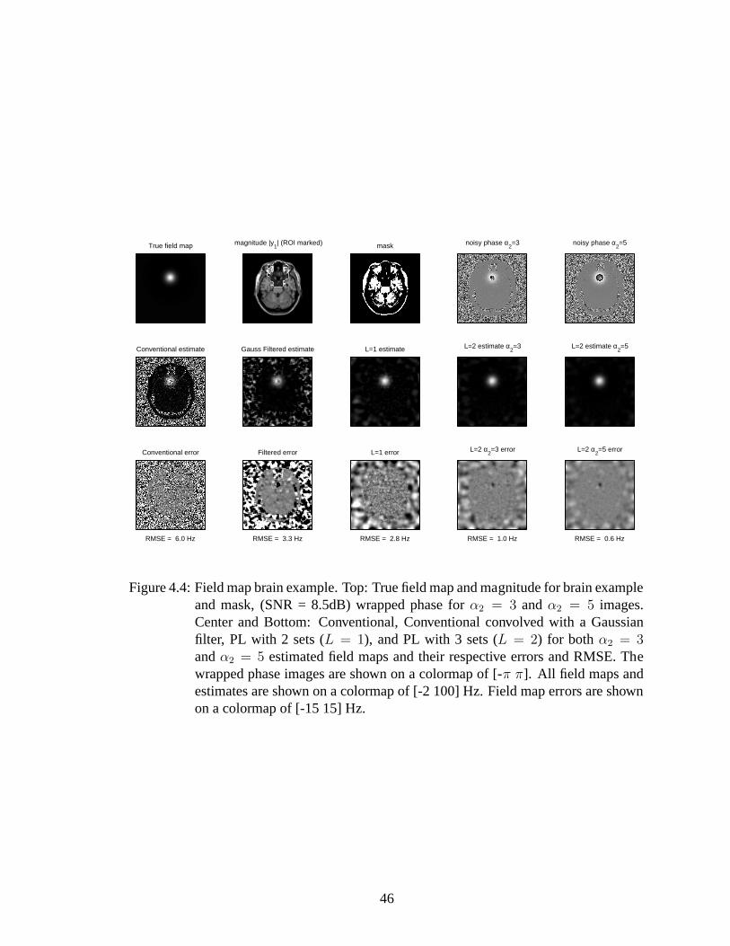
True field map magnitude |y1| (ROI marked) mask noisy phase α

2=3 noisy phase α

2=5

Conventional estimate Gauss Filtered estimate L=1 estimate L=2 estimate α2=3 L=2 estimate α

2=5

Conventional error

RMSE = 6.0 Hz

Filtered error

RMSE = 3.3 Hz

L=1 error

RMSE = 2.8 Hz

L=2 α2=3 error

RMSE = 1.0 Hz

L=2 α2=5 error

RMSE = 0.6 Hz

Figure 4.4: Field map brain example. Top: True field map and magnitude for brain exampleand mask, (SNR = 8.5dB) wrapped phase forα2 = 3 andα2 = 5 images.Center and Bottom: Conventional, Conventional convolved witha Gaussianfilter, PL with 2 sets (L = 1), and PL with 3 sets (L = 2) for bothα2 = 3andα2 = 5 estimated field maps and their respective errors and RMSE. Thewrapped phase images are shown on a colormap of [-π π]. All field maps andestimates are shown on a colormap of [-2 100] Hz. Field map errors are shownon a colormap of [-15 15] Hz.

46

The SNR remains consistent even when varyingR∗2, L, orα.

We used1 = 2 msec for both cases. For theL = 2 case we also variedα2 to

produce several2 values. We used a uniform value ofR∗2 = 20 sec−1 in generating our

simulations.

The field map was reconstructed using the penalized-likelihood method (4.11) using

normalization as described in Section 4.2.8 for bothL = 1 andL = 2. The algorithm

(4.13) was run at each SNR level for theL = 1 case and for theL = 2 case of data with

varying values ofα2 using 5 realizations. We ran 300 iterations of the algorithm, using

β = 2−3.

We also applied the conventional estimator to our data. To reduce the noise, we

convolved the conventional estimate with Gaussian filters of varying widths (σ =

0.0625, 0.1250, . . . , 3.125). We chose the “optimal”σ based on the minimum masked

RMSE. Choosing the optimalσ using the true field map gives the conventional estimate

an advantage in this example unavailable in practice.

The RMS error (in Hz) was computed between the “true” field mapand the field map

reconstructed using the PL method (4.11) and the conventional estimate. This RMSE was

calculated in a masked region (pixels with magnitudes at least 20% of the maximum true

magnitude).

Fig. 4.3 shows an example of the PL withL = 1 estimate compared to the PL with

L = 2 estimate atα2 = 3 andα2 = 7 at an SNR of 10dB. Qualitatively, we can see

improvements with increases in bothL andα2. Fig. 4.4 shows similar results for the brain

example.

The largest errors in these field maps occur where the magnitude is smallest. The RMSE

is much higher using only the conventional method. We also calculated the RMSE in the

sinus region of the brain (the ROI is shown in Fig. 4.4). We chose this ROI because the low

magnitude makes the field map difficult to estimate here although the field inhomogeneity

is also greatest here. The RMSE in this ROI was 61.1 Hz for the conventional estimate, 11.6

47

Hz for the Gaussian filtered estimate, 3.4 Hz for theL = 1 regularized estimate, and 1.9

Hz for theL = 2 α2 = 3 regularized estimate and 1.7 Hz for theL = 2 α2 = 5 regularized

estimate. Overall, the filtered conventional estimate performed similar to the PL method

with L = 1 over the masked region, but had higher error in the ROI. The PLmethod

with L = 2 showed a decreased error in both the masked region and the ROI. We would

expect even higher improvement over any practical Gaussianfiltered estimate because a

suboptimalσ would be used. The proposed regularized estimators are moreaccurate in

pixels with low magnitude. Adding additional scans (L > 1) makes the PL estimate even

more accurate.

Fig. 4.5 shows the improvement (defined as the RMS error for PLestimate withL = 1

divided by the error for PL estimate withL = 2) gained by using an additional set of data

for the Gaussian example. For comparison, we also plotted the predicted improvement,

given by the square root of the ratio of the expressions (4.19) and (4.20). The experimental

gains are actually higher than the improvements anticipated as shown by the dotted lines

(the predicted improvement) for some SNR values. Because this is a ratio of RMSEs and

the amount of bias can vary betweenL = 1 andL = 2, the unbiased CRB provides a

benchmark of expected ratios rather than an exact upper limit. Also, recall that (4.19) and

(4.20) consideredR∗2 to be a known value when, in fact,R∗

2 is unknown and approximated

through (4.9). The RMSE is low (in voxels with large magnitudes) at high SNRs using

eitherL = 1 orL = 2. At lower SNRs, however, including in voxels with low magnitudes,

usingL = 2 and higher values ofα2 greatly reduces RMS error. We repeated these sim-

ulations withR∗2 = 0 (results not shown) and the empirical improvement almost exactly

matched (4.18).

Fig. 4.6 shows the improvement gained by using an additionalset of data for the brain

image. For a low SNR (for example 10 dB), the improvements areclose to expected. The

brain image has some areas where the magnitude is very low, making estimation using any

method quite challenging. In addition, the field map phase itself is less smooth than in the

48

0 5 10 15 20 251

2

3

4

5

6

7

SNR [dB]

Impr

ovem

ent R

atio

RMSE improvement over 2 sets for Gauss data, R2* =20 sec−1

α2 = 7

Expected α2 = 7

α2 = 5

Expected α2 = 5

α2 = 3

Expected α2 = 3

α2 = 1

Expected α2 = 1

Figure 4.5: Improvement in the RMSE for the Gaussian exampleby using 3 data sets ratherthan 2 sets. Expected improvements shown by dotted lines.

49

0 5 10 15 20 251

2

3

4

5

6

7

SNR [dB]

Impr

ovem

ent R

atio

RMSE improvement over 2 sets for Brain data, R2* =20 sec−1

α

2 = 7

Expected α2 = 7

α2 = 5

Expected α2 = 5

α2 = 3

Expected α2 = 3

α2 = 1

Expected α2 = 1

Figure 4.6: Improvement in the RMSE for the brain example by using 3 data sets ratherthan 2 sets. Expected improvements shown by dotted lines.

50

Gaussian case, making the estimation more difficult. For a higher SNR (for example 20

dB), the 3-set case still outperforms the 2-set case substantially but by less than predicted

by (4.18).

The RMSE has components of both bias error and variance in it,as shown below:

RMSE(X) =

√VarX+bias2(X).

Therefore, we analyzed the bias and the standard deviation at a single representative SNR

= 20 dB and atα2 = 1, 2, . . . 7 using 500 iterations and 100 realizations for each factor.

Fig. 4.7 compares the standard deviation for eachα2 relative to that atα2 = 1 and the empir-

ical improvements were compared to those predicted by the CRB(4.20) for the Gaussian

example. As expected, the improvements in variance are veryclose to predicted. Here, the

bias is also very low at all levels of SNR - explaining the improvement seen in RMSE in

Fig. 4.7.

Fig. 4.8 shows the bias and standard deviation for a signle SNR = 20 for the brain exam-

ple. The empirical variances were close to those expected. The bias, however, introduced

in part by the regularization, was nearly constant (independent ofα). So for large values of

α2, the bias begins to dominate the variance in RMSE calculations, explaining Fig. 4.6.

Overall, the variance reductions in both examples due to using three echo times were

close to the results predicted by the CRB. For low values ofα2 (i.e., five or less), the ex-

pected benefit usingL > 1 holds even with a moderate value ofR∗2. The RMSE reductions

are largest at lower SNRs. For phase estimation, the local SNR depends on the spin density

of each voxel as seen in (4.17). Voxels with lower spin density effectively have lower SNR.

It is precisely in these voxels where using 3 or more scans hasthe greatest benefit.

51

1 2 3 4 5 6 70

0.5

1

1.5

2

2.5

3Space Averaged σ and |Bias|

k1

[Hz]

σ|bias|

2 2.5 3 3.5 4 4.5 5 5.5 6 6.5 71

2

3

4

5

6

7

k1

Impr

ovem

ent

Improvement in σ over α2=1

improvement (σ)

expected improvement (σ)

Figure 4.7: Bias and RMSE improvement for Gaussian example.Top: Space-averagedσand absolute bias for severalα2 values; Bottom: RMSE improvement, empiri-cal and expected, overα2 = 1 for severalα2 values.

Table 4.1: Phantom NRMSE for two representative slicesPhantom NRMSE (%) for one realization

Slice One Slice ThreeWhole Image Low Magnitude Whole Image Low Magnitudeµ σ µ σ µ σ µ σ

No Field Map 31.1 - 4.8 - 20.4 - 2.9 -Conventional 15.0 0.5 6.8 0.6 15.5 0.2 2.2 0.1Gauss Filter 14.3 0.4 6.1 0.4 15.1 0.2 1.9 0.08L=1 13.0 0.4 4.0 0.4 15.2 0.2 1.8 0.04L=2 α2 = 2 13.1 0.4 4.1 0.4 14.8 0.1 1.8 0.03L=2 α2 = 5 13.5 0.08 4.3 0.2 14.6 0.02 1.8 0.01L=3 13.5 0.09 4.4 0.1 14.6 0.02 1.8 0.01

52

1 2 3 4 5 6 70

0.5

1

1.5

2Space Averaged σ and |Bias|

k1

[Hz]

σ|bias|

2 2.5 3 3.5 4 4.5 5 5.5 6 6.5 71

2

3

4

5

6

k1

Impr

ovem

ent

Improvement in σ over α2=1

improvement (σ)

expected improvement (σ)

Figure 4.8: Bias and RMSE improvement for brain example. Top: Space-averagedσ andabsolute bias for severalα2 values; Bottom: RMSE improvement, empiricaland expected, overα2 = 1 for severalα2 values.

53

|x| (8 shot) Conventional Gauss Filter L = 1 L = 2 α2 = 2 L = 2 α

2 = 5 L = 3 Field map

|x| (1 shot) conventional Filtered L = 1 L = 2 α2 = 2 L = 2 α

2 = 5 L = 3

Figure 4.9: MR phantom data field map reconstructed using proposed method. First Slice- Top: Reconstructed 8-shot image, Conventional field map, Gaussian filteredfield map, regularized field map L=1, regularized field map L=2; α2 = 2, reg-ularized field map L=2α2 = 5, regularized field map L=3. The field mapsare displayed with a common color scale from -35 Hz to 50 Hz; Bottom: Re-constructed one-shot image with no field map and with each of the field mapsabove. The images are all on the same color scale. These are all from onerepresentative realization.

4.3.2 MR phantom data: Application to Spiral Trajectories

To illustrate how improved field map estimation leads to improved reconstructed im-

ages, we used field maps produced by the conventional method (4.2) and produced by the

PL method with three scans (4.11) to correct real spiral MR data for field inhomogeneities.

We imaged a phantom with large field inhomogeneity. We used a spiral-out trajectory with

a TE of 30 ms, TR of 2 sec, and a flip angle of 90 degrees. We took six slices spaced 5 cm

apart over the 15 cm field of view. First, we collected data to create the field maps (using

eight interleaves to minimize the effect of the field inhomogeneity) at the original 30 ms,

as well as at 32 ms (1 = 2 ms) and at 34 ms (2 = 4 ms) and at 40 ms (2 = 10 ms).

We took ten realizations for each echo difference. We reconstructed iteratively the result-

ing 64 × 64 pixel images in a masked region using [36]. Then, we used these images to

create (for each slice) a conventional field map (4.2), a conventional field map blurred with

a Gaussian filter, a PL field map withL = 1, a PL field map withL = 2 andα2 = 2, a PL

field map withL = 2 andα2 = 5, and a PL field map withL = 3, (4.11). We usedβ = 2−6

54

for the regularized iterative algorithm andσ = .5 for the Gaussian filter approach, approx-

imately matching the FWHM of the two approaches. Finally, we collected one-shot spiral

out data with TE = 30 ms. This scan is thus much more affected byfinal inhomogeneity.

We collected two realizations and then averaged them in k-space. We first reconstructed

this data iteratively without a field map as in [36]. Uncorrelated field inhomogeneity causes

a blurred image for spiral trajectories. Finally, we iteratively reconstructed this one-shot

data with each of the field maps previously created as in [114].

Fig. 4.9 shows one representative slice. The regularized field maps are less noisy than

the conventional one, especially in areas of low magnitude and along the edges. Fig. 4.9

illustrates the blur and distortion in the one-shot image reconstructed without a field map.

The images reconstructed with a field map do not have this blur. Nevertheless, a noisy

field map can cause error in the reconstructed image. For example, in Fig. 4.9, the image

reconstructed with the conventional field map shows more artifacts than the eight-shot data

or either of the images reconstructed with regularized fieldmaps. Using the eight-shot data

as “truth”, we computed the NRMSE of each image and Table 4.1 shows the mean and

variance over the ten realizations. We include data from tworepresentative slices to show a

range of values, although slice three is not shown. In addition, we calculated the NRMSE

in the one-shot reconstructed images in pixels where the magnitude is less than.2 times the

maximum pixel value of the eight-shot reconstructed image to see if the regularized field

maps reduce errors in areas of the image with low magnitude. This is also reported in Table

4.1. We use the norm of the eight-shot 30 ms image for normalization. The regularized

iterative PL methods have a lower RMSE and much less variability than the other methods.

Therefore, these regularized methods (especially with more than one echo time) give a very

reliable estimate of the field map with little variability.

55

4.3.3 Application to EPI Trajectories

The search for more accurate field map estimation methods is motivated by fast MR

imaging, such as echo-planar imaging (EPI) and spiral imaging used in fMRI. Because

these methods use long readout times,Bo field inhomogeneities or magnetic susceptibili-

ties become more pronounced. Without any correction for a non-uniform field, the resulting

reconstructed images will have artifacts. Using field map correction will result in an im-

proved MR image [32,74,75]. More accurate field maps, as produced using the methods in

this paper, should further decreases the artifacts, resulting in an improved final MR image.

To illustrate how improved field map estimation leads to improved images that are re-

constructed with field correction, we used field maps produced by the conventional method

(4.2) and by two scans as well as three scans (4.11) usingα2 = 5 with R∗2 = 20 sec−1

with 150 iterations, to correct simulated EPI data for field map inhomogeneities. We used

a readout length of 30ms with a matrix size of 64x64 for the simulations and used the

iterative method for reconstruction explained in [114].

Fig. 4.10 has a simple field map of a square inside an oval usingβ = 2−6. Here, RMSE

was calculated in the oval region. This simpler field map makes visual analysis of the field

maps and their errors easier to judge. Again, the conventional field map estimate has much

more noise, especially in areas of low magnitude. The two scan field map has a much more

accurate field map with lower overall RMSE. The three scan field map is also included

here. The overall error is again much lower and the image is less noisy than the two-scan

field maps.

We generated k-space data for an EPI trajectory using these simulated field maps and

a magnitude with a grid phantom. Fig. 4.11 shows the results of the field map correction

on the reconstructed image. With no field map correction, several shifts occur to the grid.

Using the true field map for the field map correction creates the true image with a clean

grid. The conventional field map, although an improvement over no field map correction,

still has large artifacts at all locations where the magnitude is small. The images using the

56

True field map

|yi|

Conventional

error

RMSE = 20.6 Hz

2 sets

error

RMSE = 6.1 Hz

3 sets α2=5

error

RMSE = 1.4 Hz

−20

0

20

40

−50

0

50

Figure 4.10: Simple field map to correct a simulated EPI trajectory. Top row: simple fieldmap and estimated field map. Bottom row: brain image and field map errorimages.

True fieldmap Conventional 2 sets 3 sets α2=5

None

NRMS = 1.58%

NRMS = 0.15%

NRMS = 0.77%

NRMS = 0.71%

NRMS = 0.36%

Figure 4.11: Grid phantom to show effects of proper field map correction. Top row: Gridphantom and estimated field maps from Fig. 4.10. Bottom row: Reconstructedimages using no field map correction; correct field map; conventional esti-mate; 2 sets estimate; 3 sets estimate withα2=5

57

two scan and the three scan field maps for the correction have less artifacts.

As can be seen in the reconstructed images, omitting corrections for magnetic field in-

homogeneities dramatically affects the final image quality. Using a simple, conventional

field map estimate corrects for some of the problems, but still introduces image artifacts,

especially in areas of very low magnitude where field map errors begin to dominate. These

images show the dramatic improvements made by an improved field map. Using the meth-

ods introduced in this paper to create more accurate field maps gives much more accurate

reconstructed images.

4.3.4 Fieldmap estimation in k-space

The methods described above estimate the fieldmap from two ormore reconstructed

images. To work well, those images should be relatively freeof artifacts, blur, and dis-

tortions, necessitating appropriate data acquisition types. For pulse sequences with long

readout times, it may be more appropriate to estimate the fieldmap directly from the raw k-

space data. A typical scenario is that we can collect two setsof k-space data, with slightly

different echo times, from which we want to estimate the fieldmap ω and the baseline

magnetizationf . A reasonable model for the data is:

E[y

(l)i

]=

∫f(~x) e−ı ω(~x)(ti+l) e−ı2π~νi·~x d~x, l = 0, 1, . . . L.

This is a joint estimation problem like that described in [115]. One can define a cost

function in terms off andω, and then alternate between holdingω fixed and minimizing

over f (using the CG method) and then holdingf fixed and minimizing overω (using

steepest descent [115] or linearization [96] or optimization transfer methods akin to [33]).

These k-space methods require considerably more computation than the image domain

methods, so one should first apply an image-domain method to get a reasonable initial

estimate of the fieldmapω.

58

4.4 Discussion

We described a regularized method for field map estimation using two or more scans:

the penalized-likelihood method (4.11). This method yields field maps that interpolate

smoothly over regions with low spin density, thereby avoiding phase outliers that plague

the conventional estimate (4.2). The method has been used with L = 1 (without full

description) in [93,115,139].

Our analysis also shows that the conventional estimate (4.2) is in fact the ML estimate,

a property that has previously gone unnoticed to our knowledge.

We also analyzed the spatial resolution properties of this method, leading to a practi-

cal procedure for choosing the regularization parameter toachieve a given desired spatial

resolution.

We studied the CRB on the variance of the estimate for this method and found that our

empirical simulation results for the PL method compared favorably, showing a reduction in

the RMSE in comparison to using only two scans.

We collected real MR phantom data and created conventional and PL estimates of the

field map which were used to reconstruct final images. The PL estimate reduces image

artifacts caused by the field inhomogeneity and has a reducedRMSE, especially in areas of

very low magnitude where the conventional estimate has manyerrors. Omitting or using

a poor field map estimate for image reconstruction can dramatically affect the final image

quality.

As noted in Section 4.2.4, our cost function assumes, as do most other field map es-

timation problems, that there is no motion between scans. While our analysis indicated

that a largerL is better in terms of variance, motion could be a problem during the larger

time required forL echo time differences. Practically,L = 1 or L = 2 are the most likely

choices forL and here motion is less likely to be an issue. If a larger number of echo dif-

ferences are desired, then the cost function could be further generalized to include a joint

estimation of the field map and rigid motion parameters.

59

We have focused here on the case of a single receive coil. It isstraightforward to

generalize the method for phased array coils,cf. [80].

Although we did not estimateR∗2, we used a simple weighting (4.9) in our algorithm to

partially account forR∗2 decay; the improvements seen over estimation with two scansare

still large, especially when using a small value ofα2.

While this method assumed the first two echo time differences were close enough to

prevent phase wrapping, this method could, with proper intialization, extend to data with

larger echo time differences and some phase wrapping. This is especially interesting at

higher field strengths where wrapping still exists at low echo time differences.

Overall, this method has potential to be a reliable estimator for MR field maps, able

to utilize many scans to produce a good estimate. The generalpenalized-likelihood ap-

proach in this work is also applicable to estimating other parametric maps in MRI, such as

relaxation maps [46] and sensitivity maps [138]. It may alsobe useful for phase unwrap-

ping problems with noisy data. In some cases, it may be preferable to use edge-preserving

regularization in (4.12), such as the Huber potential function [141].

Ultimately, this method is a tool that may help answer the main question of field map-

ping: how to best allocate scan time to achieve the most accurate field map. The preliminary

CRB analysis guides choice of echo times given a set number of scans. In future work, we

wish to further explore the relationship between number of echoes, signal to noise ratio,

and spatial resolution.

60

CHAPTER V

B+1 Map Estimation

5.1 Introduction

In 1 MRI, RF transmit coils produce non-uniformB1 field strengths, creating varying

tip angles over the field of view. In particular, asB0 increases, the RF wavelength shortens,

causing moreB1 inhomogeneity. Measured inhomogeneity ranges from 30-60%[20, 112,

120] at high field strengths (B0 ≥ 3T). In fact,B1 is inherently inhomogeneous, both in

magnitude and phase, because there is no solution to Maxwell’s equations for a uniform

RF field over a whole volume at high frequency [56]. Uncorrected, non-uniform tip angles

cause spatially varying signal and contrast in the image. The field inhomogeneity can also

degrade quantification, such as in measuring brain volumes [145].

A map of theB+1 field strength, called aB+

1 map, is essential to many methods to

help minimize and correct for this inhomogeneity. For example, tailored RF pulses such

as [102, 111] require use of aB+1 map. Other techniques, such as myocardial perfusion

imaging [59] also require aB+1 map. At high fields (≥ 3T), aB+

1 map allows for proper

pre-scan calibration [20]. In parallel transmit excitation (using a coil array),e.g., [67, 108,

134, 135, 142, 143, 145, 148], one must have a map of theB+1 field strength and phase for

RF pulse design.

A conventional approach toB+1 mapping is to collect two scans, one of which uses

1This section is based on several conference publications: [41–43].

61

twice the RF amplitude of the other,e.g., [2, 12, 20, 127, 128]. Using the double angle for-

mula, a standard method-of-moments estimator is used that ignores noise in the data. This

estimator performs poorly in image regions with low spin density. This simple approach

also does not allow for more than two angles nor does it account for more complicated

physical factors such as slice selection effects.

We propose a new approach that incorporates multiple coils and multiple tip angles as

well as accounts for noise in the model. This model also incorporates the RF excitation

pulse envelope to account for slice selection effects. The iterative regularized estimator

estimates the unknown complexB+1 map from multiple reconstructed images. The sub-

sequent sections first review the standard approach for thisproblem, and then describe our

new and improved method with examples of the improvedB+1 maps.

5.2 B+

1Map Estimation: Theory

5.2.1 ConventionalB+1 map

The double angle method (DAM), a conventional approach toB+1 mapping, uses two

scans, one of which uses twice the RF amplitude of the other. Amodel for the reconstructed

images is

yj1 = fj sin(αj) +εj1

yj2 = fj sin(2αj) +εj2,(5.1)

whereyjl denotes the complex image value in thejth voxel for thelth scan (l = 1, 2),

fj denotes the unknown object value andαj is the unknown tip angle at thejth voxel.

Estimatingαj is equivalent to estimating theB+1 field strength magnitude at thejth voxel.

62

Using the double angle formula:

E[yj2]

E[yj1]=

sin(2αj)

sin(αj)= 2 cos(αj) .

The standard estimate ofαj is a method-of-moments estimator that ignores the noise in the

data:

(5.2) αj = arccos

(1

2

∣∣∣∣yj2

yj1

∣∣∣∣).

This method has several limitations. First, it performs poorly in image regions with low

spin density,i.e., whereyj1 is small. It suffers from2π ambiguities ifαj is too large, yet

it would be sensitive to noise ifαj is too small. Additionally, repeatibility for smallαj

(under20) is poor [112]. The solution to the added noise ignored by themodel is usually

low-pass filtering, which must be fine-tuned. Low pass filtering can corrupt neighbors of

pixels with smallαj or fj values. The estimator (5.2) also does not immediately generalize

to the case where we acquire multiple scans to cover a larger range of tip angles, possibly

even angles that are larger than2π in some image regions. The estimate (5.2) also does not

provide phase information and most methods do not incorporate any phase estimate.

Finally, the estimate (5.2) does not take into account any information about the excita-

tion pulse, thus ignoring slice selection effects. The model shown in (5.1) assumes a linear

relationship between the pulse amplitude and the flip angle.Such linearity holds for a non-

selective pulses but is only an approximation for slice selective pulses. According to [110],

the linear approximation is adequate for sinc pulses up to 140 degrees, but using a non-ideal

pulse such as a Gaussian would decrease the accuracy even further. The effects of using

a finite pulse also cause residual error, but are not accounted for in published methods.

Different slice profiles affect the aboslute flip angle as well as the flip angle distributions

throughout the sample [126].

The model (5.1) usually requires a very large TR so thatfj is the same for bothyj1

63

andyj2 (i.e., the effects of bothT1 andT2 relaxation are negligble). For an object with a

knownT1 value or knownT1 map, one can generalize the model (5.1) to include the effects

of T1, e.g., [143]. Some papers, such as [128], using the conventional model (5.1) suggest

that shorter TR values can be used. Sequences have been suggested that can shorten scan

time and enable rapidB+1 mapping, such as [20]. Some fast methods have been developed

that concurrently estimate or correct theB1 field, (e.g., [24]) to circumvent the difficulty

of a quick direct mapping. Some methods have been developed that are “T1 oblivious”

over the relevant range ofT1 values (e.g., [39]) to circumvent needingT1 information at all.

All currentB+1 mapping have disadvantages that need to be corrected (e.g., flow artifacts,

off-resonance, suceptibility effects), but most have low noise and low bias [81]. Because

the proposed method is built around a very general cost function, it is also applicable to

fast methods developed for the DAM.

Our proposed method seeks to map both the magnitude and phaseof theB1 field. This

method uses a statistical cost function that incorporates noise and slice selection effects

ignored by the conventional estimate. Including regularization into our cost function also

circumvents the need for later filtering.

5.2.2 Signal model for multiple coils, multiple tip angles/coil combinations

Suppose there areK coils. We takeM measurements by transmitting with different

coil combinations and receiving from a common coil. (This method could be generalized

to use multiple receive coils.) For each measurement, one ormore coil(s) are driven si-

multaneously by the same RF signalb1(t) with possibly different known amplitude scaling

factorsαmk, wherek = 1, . . . , K denotes the coil number,m = 1, . . . ,M denotes the

measurement number, andαis aM ×K array containing the scaling factorsαmk. For the

problem to be tractable, we require thatM > K. The complex coil patterns sum together

due to linearity to make the total transmittedB1 field. This general model encompasses the

64

conventional model (5.1) if we letK = 1,M = 2, and

α =

1

2

.

We model the resultingM reconstructed images as follows:

(5.3) yjm = fjF

(K∑

k=1

αmkzjk

)+ εjm,

for m = 1, . . . ,M andj = 1, . . . , N , wherefj denotes the underlying object transverse

magnetization in thejth voxel (multiplied by the sensitivity of the receive coil)andεjm

denotes zero-mean complex gaussian noise. TheB+1 map, constrained to be real in the

conventional model, is actually a complex quantity.zjk denotes the unknown complexB+1

map that relates RF amplitude to tip angle at thejth voxel for thekth coil. When multiple

coils are driven by the same signalb1(t) (with possibly different amplitudes), then the fields

from those coils will superimpose and the complex coil patterns will add by linearity, hence

the sum overk in (5.3). If the units of the amplitudesαmk are gauss, then the units ofzjk

will be radians per gauss. More typically, the units ofαmk are arbitrary, and all that is

known is their relative values. In this casezjk will have units such that the product ofαmk

andzjk has units of radians. This should suffice for RF pulse design.

The functionF in (5.3) replaces the typicalsin seen in the double angle formula and

inherently incorporates slice selection effects. The function F is explained further in Ap-

pendix B.

The model (5.3) expands the one used in [41, 42] and includes both slice selection ef-

fects and linear transceive coil combinations. RecentB1 mapping methods [10, 90] have

introduced linear combinations of transmit coils. These methods have the advantage of us-

ing much smaller tip angles while still collecting enough signal to produce accurate results.

The proposed method accomodates this matrix transmit technique with a comprehensive

65

measurement model that also includes slice selection effects and accounts for the noise

factors that are ignored by existing methods.

The goal is to estimate eachB+1 map zk , (z1k, . . . , zNk) from the reconstructed

imagesyjm. The underlying magnetizationf , (f1, . . . , fN) is also unknown but is a

nuisance parameter. We would like the estimator to work robustly even in image regions

wherefj is small.

If fj were allowed to be complex, then the model above would be non-identifiable so

we take the approach of constrainingf to be real.

We also note a single surface coil for receive will suffice, even when multiple transmit

coils are used. In this case,f will be a product of the spin density and the receive coil

sensitivity pattern.

Kerr et al. [68] considered a similar problem, except they assumedαmk values are

powers of two,F was the ideal sin relationship, andz was a real quantity. They did not use

coil combinations, so each row ofα would correspond to an indicator function. They used

the following cost function:

∑

j,m

(|yjm| − |fj| sin(|αmkzjk|))2 .

This cost function does not correspond to the complex gaussian statistical model for the

data. They applied a general purpose minimization method from MATLAB . In particular

for simplicity, for each voxel they used only the value of tipindex for which the tip was

closest toπ/2. They also applied no regularization. In contrast, we use all the data at

every voxel, with a statistically motivated cost function,and a minimization algorithm that

is tailored to this problem. We allow arbitrary choices for theαmk values, although powers

of two may be a reasonable choice. We use the Bloch equation toaccomodate real pulse

sequences instead of assuming a perfect rectangular slice profile.

66

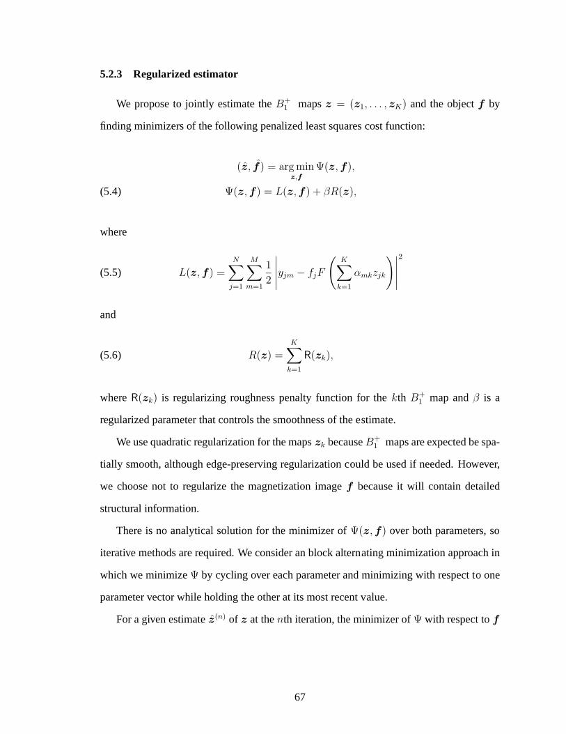
5.2.3 Regularized estimator

We propose to jointly estimate theB+1 mapsz = (z1, . . . ,zK) and the objectf by

finding minimizers of the following penalized least squarescost function:

(z, f) = arg minz,f

Ψ(z,f),

Ψ(z,f) = L(z,f) + βR(z),(5.4)

where

L(z,f) =N∑

j=1

M∑

m=1

1

2

∣∣∣∣∣yjm − fjF

(K∑

k=1

αmkzjk

)∣∣∣∣∣

2

(5.5)

and

R(z) =K∑

k=1

R(zk),(5.6)

whereR(zk) is regularizing roughness penalty function for thekth B+1 map andβ is a

regularized parameter that controls the smoothness of the estimate.

We use quadratic regularization for the mapszk becauseB+1 maps are expected be spa-

tially smooth, although edge-preserving regularization could be used if needed. However,

we choose not to regularize the magnetization imagef because it will contain detailed

structural information.

There is no analytical solution for the minimizer ofΨ(z,f) over both parameters, so

iterative methods are required. We consider an block alternating minimization approach in

which we minimizeΨ by cycling over each parameter and minimizing with respect to one

parameter vector while holding the other at its most recent value.

For a given estimatez(n) of z at thenth iteration, the minimizer ofΨ with respect tof

67

is found analytically to be:

(5.7) fj

(n)=

∑Mm=1 real

y∗jmF (x

(n)jm)

∑Mm=1

∣∣∣F (x(n)jm)∣∣∣2 ,

where we define the compositeB+1 mapsxm as follows:

(5.8) xjm ,

K∑

k=1

αmkzjk.

For givenf values, the problem of minimizingΨ with respect to the complexB+1 map

zm appears nontrivial because of the nonlinearity ofF . Therefore, we use an iterative

algorithm of the following form:

z(n+1) = z(n) −D(z(n), f (n))∇z Ψ(z(n), f (n)

),

whereD is a diagonal matrix that is derived using quadratic majorizer principles [8] to

ensure that the cost functionΨ is decreased each iteration. See Appendix C for details.

Variable projection is another possible approach (see [48,54,109]) where we substitute

the linear solution off (5.7) back into the cost function (5.4) and then find an estimator

for z. However, we found no simplifications in (5.4) in using (5.7); so we use alternating

minimization. The cost functionΨ is nonconvex, so the alternating minimization

algorithm described above will descend from the initial estimates to a local minimum [63].

Thus it is desirable to choose reasonable initial estimates. See Appendix E for details.

Regularized methods have the benefit of being able to choose avalue forβ based on

quantitative analysis. In Appendix G, we analyze the spatial resolution of the regularized

estimator (5.4). This analysis leads to a modified penalty function which achieves more

uniform spatial resolution in regions with a constantfj. We choose a value forβ based on

the desired FWHM of regularizer smoothing.

68

5.3 Experiments

5.3.1 Simulation Study

object

1 64

1

62 0

200

B1 maps

1 64

1

62 0

0.839

Phase maps

1 64

1

62 0.803

1.56

Figure 5.1: TrueB+1 magnitude and phase maps and object used in simulation.

Scan for y_1

1 64

1

62

Scan for y_2

1 64

1

62

Scan for y_3

1 64

1

62

Scan for y_4

1 64

1

62

Scan for y_5

1 64

1

62

Scan for y_6

1 64

1

62

Scan for y_7

1 64

1

62

Scan for y_8

SNR = 20.0 dB1 64

1

62

Figure 5.2: Simulated MR scans for leave-one-coil-out (LOO). Estimation withM = 8measurements and with an SNR of 20dB.

69

To evaluate the regularizedB+1 map estimation method described above, we performed

a simulation study using the synthetic true maps shown in Fig. 5.1. For the object magni-

tudefj, we used a simulated normal T1-weighted brain image [18, 70]for the truth. The

B+1 maps were simulated based on equations for a magnetic field ina circular current

loop [49, 129]. We simulated noisy reconstructed images forK = 4 different transmit

coils using the model (5.3) and varying both the number of measurements (M = 2K

or M = K + 1), α, and the RF pulse (truncated gaussian and truncated sinc, see Ap-

pendix B for details). For our scaling matrixα, we used “one-coil-at-a-time” (OAAT) (i.e.,

for M = 2K

αOAAT =

IK

2 · IK

,

whereIK is aK ×K identity matrix) and “leave-one-coil-out” (LOO) (i.e., forM = 2K

αLOO =

1K − IK

2 · 1K − 2 · IK

,

where1K is aK × K matrix of ones). There are many possible choices forα, but we

focus on these two possible matrices as an illustration of the method. Both matrices are

well-conditioned (κ (αOAAT) = 1 andκ (αLOO) = 3). All choices forα in this paper meet

the criteria of the modified DAM used in Appendix E in calculating z(0). We just show

images for the truncated sinc pulse as images from both excitation pulses look similar. We

added complex gaussian noise such that the SNR, defined by10 log10(‖y‖/‖y − E[y]‖),

was about 20 dB whenM = 2 ·K and about 30 dB whenM = K + 1. Fig. 5.2 shows the

data magnitude|yjm| scans for LOO atM = 8.

Fig. 5.3 and Fig. 5.4 show the initial estimates, regularized estimates and their respec-

tive errors using the methods described in Appendix E for theusualM = 8 case. Both the

conventional DAM estimate for|z| and the method of moment estimate for∠z are quite

noisy. For the first pass through the algorithm, we ran 5 iterations and usedβ1 = 2−10

70

DAM est. Reg. est. (abs)

Masked init. error Masked reg. error

DAM (phase) est. Reg. est. (phase)


Figure 5.3: Figures for one coil at a time (OAAT). 500 iterations, M=8, SNR about 20 dB,β = 2−1, Same figure colorbar as Fig. 5.1. Error colorbar is [-.07, .07] for |z|and [−π/8, π/8] for ∠z

71

DAM est. Reg. est. (abs)


DAM (phase) est. Reg. est. (phase)


Figure 5.4: Figures for 3 coils at a time (LOO). 150 iterations, M=8, SNR about 20 dB,β = 2−1, Same colorbar as Fig. 5.3.

72

and used the modified penalty as described in Appendix G. The data was also normalized

by the median of the first pass estimate of the object as described in Appendix G. We ran

the algorithm with 150 iterations, usingβ = 2−1 and using the modified penalty (G.7).

The algorithm, including the first pass, took 300 seconds to run on Matlab. Fewer iteration

could be run (whenM = 2K) to further speed up processing - all estimates have less than

10% NRMSE at 75 iterations, for example, which would almost halve the run time.

The reduced noise due to regularization and due to using all the scan data is evident.

Fig. 5.3 shows the conventional estimate for theB+1 map. Not only is this image very

noisy, but theB+1 map is not properly estimated in the large signal void of the skull. This

is expected from the very low tip angles that are used here (about 20 degrees in the center

for the first four scans and about 40 degrees in the center for the next four scans). We

see some improvement in Fig. 5.4 even in the initial estimates because using three coils

at a time brings the center tip to around 60 degrees for the first four scans and about 120

degrees for the next four scans, making the DAM much better conditioned and less prone

to error. The proposed method improves over the initial estimate for both the OAAT and

LOO cases. It smoothly interpolates across this signal voidfor a smoothB+1 map in the

region of interest as seen in Fig. 5.3 and Fig. 5.4. Similarly, signal voids can be seen in the

initial estimate of the phase map yet are smoothed appropriately in the final estimate.

We calculated the error of both the conventional and our new estimate for all four coils.

We used a mask to include only those points where the signal value is non-negligible (i.e.,

where|fj| > 0.1 max (fj)). For error in the phase of theB+1 map, we looked at

∣∣eiz − eiz∣∣.

The results are summarized in Table 5.1, where the errors areaveraged over 20 realizations

(the variance of the error over the realizations is very small, less than one percent). The

error in the new regularized estimate for theB+1 magnitude is three to five times less than

the error of the conventional estimate. OAAT has greater improvements due to the very

poor DAM estimate at such low flip angles. The phase estimate and object estimate (not

shown) are similarly good. This clearly shows the effects ofless noise and interpolating

73

Table 5.1: Simulation NRMSE (%) for three selected excitation pulses averaged over 20realizations

|z|(0) |z|(n)∠z(0) ∠z(n) SNR # iters

Trunc. sinc pulseOAAT M = 8

fj > 0.1 max fj 77.0 15.5 17.4 3.1 20 150

Low Magnitude 143.2 19.3 63.8 2.7 20 150Gaussian pulseOAAT M = 8

fj > 0.1 max fj 78.3 16.4 16.0 3.1 20 150

Low Magnitude 143.3 22.9 61.7 2.7 20 150Ideal sinc pulseOAAT M = 8

fj > 0.1 max fj 67.6 13.6 13.6 2.5 20 150

Low Magnitude 134.8 18.0 57.1 2.3 20 150

Trunc. sinc pulseLOOM = 8

fj > 0.1 max fj 17.4 4.9 28.5 6.7 20 150

Low Magnitude 58.7 3.9 77.7 7.0 20 150Gaussian pulseLOOM = 8

fj > 0.1 max fj 26.8 8.3 29.1 5.5 20 150

Low Magnitude 64.0 7.0 77.6 5.5 20 150Ideal sinc pulseLOOM = 8

fj > 0.1 max fj 14.1 3.9 24.2 5.4 20 150

Low Magnitude 52.4 3.2 70.8 5.5 20 150

across the signal voids. Similarly, we looked at the error inthe signal voids of the brain

(the sinuses and skull) to see the improvement even more clearly. These results are also

shown in Table 5.1 in the rows labeled “Low Magnitude”. The areas with low magnitude

have much greater error (almost 2 times greater) than areas with higher signal magnitude in

conventional estimators. Using the regularized estimator, the final error in pixels with low

signal magnitude is similar to that of the other pixels, yielding an error six to fifteen times

less that of the conventional error in low magnitude pixels.Thus, the regularized estimator

makes impressive improvements, especially in the signal voids.

The flexibility of the signal model and regularized estimator introduced in this paper

allows for less than the standardM = 2K scans required by the DAM, for example. We

requireM ≥ K + 1 to properly estimate both theK coil maps as well as the object. We

initialize this method as described in Appendix E; this estimate is much worse for those

coils which do not have a double angle initial estimate when we are using each coil sepa-

74

Initial est. Reg. est. (abs)

Masked initial error Masked reg. error

Initial (phase) est. Reg. est. (phase)


Figure 5.5: Figures for 3 coils at a time (LOO) with less measurements. 1000 iterations,M=5, SNR about 30 dB,β = 2−4, Same colorbar as Fig. 5.3.

75

Initial est. Reg. est. (abs)

Masked initial error Masked reg. error

Initial (phase) est. Reg. est. (phase)


Figure 5.6: Figures for one coil at a time (OAAT) with less measurements. 200 iterations,M=5, SNR about 30 dB,β = 2−4, rotate initial estimate from first coil forsubsequent coils. Same colorbar as Fig. 5.3.

76

rately and the estimate is quite poor for all the coils when weuse multiple coils at a time

because we lack enough information to ascertain each coil’sindividual map. Even in these

conditions, as long as the coils overlap enough to provide good coverage of the object,

the estimator will provide a good solution. However, the regularized estimator takes many

more iterations to converge to a good solution, the cost of having fewer scans. At low SNR,

the object andB+1 estimates have more “holes” in them and the regularized estimator is es-

pecially prone to being caught in a local minima. This is especially problematic for OAAT-

with less coil overlap, the initial estimate forM = 5 has many “holes” at an SNR less than

65 dB. Therefore, when using reduced number of scans, LOO is recommended, especially

at low SNR. However, OAAT and LOO can be improved by using an increased number of

scans (M = 6, for example) or by rotating the initial estimate for the coil (or coil combina-

tion) with two scans for the other coil (or combination) initial scans. Because the simulated

coil maps used here are simply rotations of each other, this simple step gives good perfor-

mance for even OAAT at an SNR of 30 dB with only 200 iterations (shown in Fig. 5.6).

This is impressive considering that the algorithm performed very poorly at this low SNR

without the initial coil rotation. Thus, using additional information or assumptions about

the coil maps can lead to a significantly reduced number of scans.

The initial and final estimates forM = 5 LOO with 1000 iterations at an SNR of 30 is

shown in Fig. 5.5 withβ = 2−4. We chose a slightly lowerβ for the low scan simulations to

put more emphasis on the likelihood term (versus the penaltyterm). The initial magnitude

and phase estimates are identical for each coil (as explained in Appendix E). The initial

magnitude estimate is quite uniform across the object; as the algorithm iterates, the varia-

tion across theB+1 magnitude map for each individual coil is corrected and approaches a

good, regularized solution. While there is still more high value error for the magnitudeB+1

estimate, this can be further reduced using more iterations. The phaseB+1 estimate is very

good and reaches a good solution with low error quickly.

The results forM = 5 LOO, at an SNR of 30 at 250, 500, and 1000 iterations are

77

compared to the conventional DAM method usingM = 8 scans in Table 5.2. Note that

the initial magnitude error withM = 5, which uses the DAM estimate for the first coil

combination for all coil combinations, is not equal to the DAM magnitude error withM =

8. We use the MOM phase estimate (E.1) for the DAMM = 8 phase estimate. The DAM

M = 8 at an SNR of 30 has a low error in high magnitude pixels (6%), but a much higher

error in low magnitude pixels (32%). After 1000 iterations,we achieve a similar degree

of error in low magnitude pixels (9%) and substantially reduce error in the low magnitude

pixels (8%) giving a similar error rate in all pixels within the object mask. Phase error is

lower for all number of iterations shown for the proposed method withM = 5 than for the

MOM M = 8 estimator and is substantially lower in low magnitude pixels (by a factor of

10).

The OAAT coil combinations failed to provide good results with only 5 scans at an SNR

of 30dB with the standard initialization. However, when we rotated the initial estimate

for the first coil for the subsequent coils as explained above, the estimator provided good

estimates with a much reduced number of iterations. Rotation of the oval brain shape

caused more error along the edges of the oval, but overall theproposed method coped with

the object shape irregularities quite well for OAAT (under the present implementation, the

coil combinations used in LOO did not perform well with this rotation method). The final

image using 200 iterations for this method is shown in Fig. 5.6 and error results in Table

5.2. OAAT has similar trends to LOO, but has significantly better results than the OAAT

DAM M = 8 estimates. Because OAAT uses only one coil at a time, the achieved flip

angles achieved are much lower and the OAAT DAM estimate has more initial error than

that of LOO DAMM = 8 estimate. Therefore, the regularization of the proposed method

substantially decreases the error, especially in low magnitude pixels.

Thus, using only 5 scans as opposed to the standard 8, produces similar (for LOO) or

lower (for OAAT) NRMSE in high magnitude pixels and substantially lowered error in

low magnitude pixels, albeit at the price of a high number of iterations. Optimization of

78

Table 5.2: Simulation NRMSE (%) for proposed methodM = 5 versus conventionalDAM methodM = 8 averaged over 20 realizations (truncated sinc pulse withSNR=30dB)

|z|(0) |z|(n)∠z(0) ∠z(n) # of iters

LOOM = 5 proposed fj > 0.1 max fj 43.5 19.9 12.2 4.0 250Low Magnitude 49.4 22.8 25.7 4.8 250fj > 0.1 max fj 43.5 13.2 12.2 3.8 500Low Magnitude 49.4 13.5 25.7 4.3 500fj > 0.1 max fj 43.5 9.1 12.2 3.4 1000Low Magnitude 49.4 8.0 25.7 3.7 1000

LOOM = 8 DAM fj > 0.1 max fj 5.8 11.1Low Magnitude 31.6 45.2

OAAT M = 5 proposed fj > 0.1 max fj 80.5 17.3 35.5 8.4 50Low Magnitude 122.7 24.5 54.8 7.4 50fj > 0.1 max fj 80.5 15.9 35.5 5.9 100Low Magnitude 122.7 24.5 54.8 3.3 100fj > 0.1 max fj 80.5 14.6 35.5 4.9 200Low Magnitude 122.7 22.1 54.8 2.7 200

OAAT M = 8 DAM fj > 0.1 max fj 58.1 17.7Low Magnitude 116.8 59.3

this method (for example, improving the initial estimate based on information about the

relative coil patterns as suggested above) may yield even greater improvements in reduced

scan regularized estimation.

We tested the improvement seen by using the correct slice profile for estimation versus

assuming an ideal sinc pulse profile. The results are summarized in Table 5.3. We see that

using the correct slice profile gives slightly better error results for OAAT for the truncated

sinc pulse (though curiously not for the gaussian pulse). This holds true for pixels with a

high signal value as well for signal voids. We would not expect a very large difference for

OAAT, because the flip angles are very small and the difference in F at these flip angles

is also small. For LOO we see bigger relative differences, especially among the gaussian

pulse. This is as we would expect, as the gaussian pulse differs greatly from the ideal sinc

pulse at the flip angles seen in LOO. Thus, the improved slice profile is most advantageous

at higher flip angles.

79

Table 5.3: Simulation NRMSE (%) using the correct slice profile for estimation versus using the conventional ideal pulseprofile forestimation

Excitationpulse

Assumedpulse

α |z|(0) |z|(n)∠z(0) ∠z(n) SNR # iters

Trunc sinc Trunc sinc OAAT M = 8 fj > 0.1 max fj 77.0 15.5 17.4 3.1 20 150Trunc sinc Ideal sinc OAAT M = 8 fj > 0.1 max fj 77.0 16.7 17.4 2.7 20 150Trunc sinc Trunc sinc OAAT M = 8 Low Mag 143.2 19.3 63.8 2.7 20 150Trunc sinc Ideal sinc OAAT M = 8 Low Mag 143.2 21.0 63.9 2.6 20 150

Gaussian Gaussian OAAT M = 8 fj > 0.1 max fj 78.3 16.4 16.0 3.1 20 150Gaussian Ideal sinc OAAT M = 8 fj > 0.1 max fj 78.3 10.8 16.0 2.8 20 150Gaussian Gaussian OAAT M = 8 Low Mag 143.3 22.9 61.7 2.7 20 150Gaussian Ideal sinc OAAT M = 8 Low Mag 143.3 12.0 63.7 2.7 20 150

Trunc sinc Trun sinc LOOM = 8 fj > 0.1 max fj 17.4 4.9 28.5 6.7 20 150Trunc sinc Ideal sinc LOOM = 8 fj > 0.1 max fj 17.4 4.7 28.4 5.9 20 150Trunc sinc Trunc sinc LOOM = 8 Low Mag 58.7 3.9 77.7 7.0 20 150Trunc sinc Ideal sinc LOOM = 8 Low Mag 58.7 4.6 77.6 6.4 20 150

Gaussian Gaussian LOOM = 8 fj > 0.1 max fj 26.8 8.3 29.1 5.5 20 150Gaussian Ideal sinc LOOM = 8 fj > 0.1 max fj 26.8 18.6 26.8 5.5 20 150Gaussian Gaussian LOOM = 8 Low Mag 64.0 7.0 77.6 5.5 20 150Gaussian Ideal sinc LOOM = 8 Low Mag 64.0 16.8 77.9 5.5 20 150

80

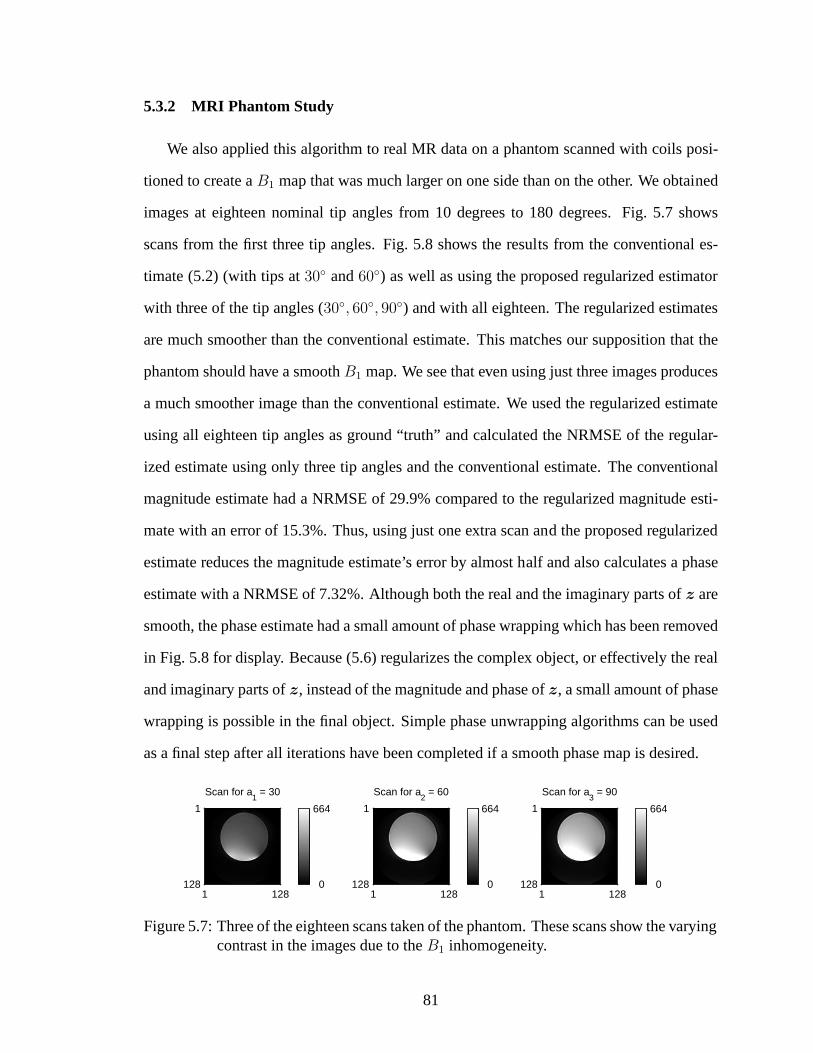
5.3.2 MRI Phantom Study

We also applied this algorithm to real MR data on a phantom scanned with coils posi-

tioned to create aB1 map that was much larger on one side than on the other. We obtained

images at eighteen nominal tip angles from 10 degrees to 180 degrees. Fig. 5.7 shows

scans from the first three tip angles. Fig. 5.8 shows the results from the conventional es-

timate (5.2) (with tips at30 and60) as well as using the proposed regularized estimator

with three of the tip angles (30, 60, 90) and with all eighteen. The regularized estimates

are much smoother than the conventional estimate. This matches our supposition that the

phantom should have a smoothB1 map. We see that even using just three images produces

a much smoother image than the conventional estimate. We used the regularized estimate

using all eighteen tip angles as ground “truth” and calculated the NRMSE of the regular-

ized estimate using only three tip angles and the conventional estimate. The conventional

magnitude estimate had a NRMSE of 29.9% compared to the regularized magnitude esti-

mate with an error of 15.3%. Thus, using just one extra scan and the proposed regularized

estimate reduces the magnitude estimate’s error by almost half and also calculates a phase

estimate with a NRMSE of 7.32%. Although both the real and theimaginary parts ofz are

smooth, the phase estimate had a small amount of phase wrapping which has been removed

in Fig. 5.8 for display. Because (5.6) regularizes the complex object, or effectively the real

and imaginary parts ofz, instead of the magnitude and phase ofz, a small amount of phase

wrapping is possible in the final object. Simple phase unwrapping algorithms can be used

as a final step after all iterations have been completed if a smooth phase map is desired.

Scan for a1 = 30

1 128

1

128 0

664

Scan for a2 = 60

1 128

1

128 0

664

Scan for a3 = 90

1 128

1

128 0

664

Figure 5.7: Three of the eighteen scans taken of the phantom.These scans show the varyingcontrast in the images due to theB1 inhomogeneity.

81

Initial estimate

1 128

1

128 0

0.229|B1+| using all tips 10−180 (gauss/waveform unit)

1 128

1

128 0

0.229

|B1+| using 30,60,90 (gauss/waveform unit)

1 128

1

128 0

0.229unwrapped phase using 30,60,90

1 128

1

128 −3.14

3.14

Figure 5.8: Estimation of the phantom using proposed method. Top: conventional estimateof B1 using two images; regularized estimate ofB1 using all eighteen images;Bottom: regularized estimate ofB1 using three images; regularized estimate ofthe phase map.

5.4 Discussion

We have described a new regularized method forB+1 mapping that estimates both the

B1 magnitude and (relative) phase. This method allows for multiple coils allowing for easy

use in designing pulse sequences for parallel excitation. This method yieldsB+1 maps that

interpolate smoothly over regions with low spin density. This avoids noisy estimates in

these regions as well as2π ambiguities that plague the conventional estimate. The conven-

tional estimate uses only two tip angles, while our method allows for any arbitrary selection

of angles.

The simulation results show that the NRMSE of the newB1 map is much less than

that of the conventional estimate. These gains make this an appropriate method even when

82

using only one coil and the standard two angles.

Although results showing the improvement made by using the correct slice profile in

the model are still very preliminary, we expect that this improvement to the model will have

a large effect at higher tip angles whereF and sin have a larger discrepancy.

This model did not account for possible coil non-linearity or possibleT1 effects. We

will explore these factors in future work.

Overall, the model and estimators explored in this paper make smoother, less noisy

estimates while also allowing for the the use of multiple coils and tip angles to achieve an

accurateB+1 and phase map for each coil.

83

CHAPTER VI

Joint B+1 , T1 Map Estimation

6.1 JointT1 andB+

1Estimation: Motivation

The longitudinal relaxation timeT1 is a quantitative value of interest in MR. Fast,

accurate, and precise mapping ofT1 has many applications: measuring the distribution

of contrast agents to find tumors or assess organs [17, 84], perfusion imaging [27, 55],

schizophrenia, epilepsy, multiple sclerosis, and Parkinson’s diagnosis [73,123,131], quan-

tifying myocardial blood flow [144], assessing lung function [64], preparing navigation

and visualization tools for surgery [50], and, in combination with accurate maps of other

parameters such asT2 and spin density, artificially creating “on the fly” MR imageswith

any desired contrast.

Moreover,T1 andB+1 mapping are usually both unknown quantities in MR pulse se-

quences. Imaging sequences for theB+1 double angle estimation method, for example,

require spin echo or gradient echo sequences with a long repetition time (TR> 5T1) to

remove anyT1 dependence from the acquired images. Fast and improved methods for the

double angle method use scan time more efficiently [20, 110, 127]. Alternatively, image

sequences which are accurate over a wide array ofT1 values have been developed [136];

these pulse sequences, however, may not give accurate phaseinformation [89]. Simple

techniques that are independent ofT1, such as finding the 180 null of the signal, do not

work well at highB0 signal strengths whereB+1 mapping is even more crucial [28] and

84

may not have good coverage over the entire volume. Ideally,B+1 estimation would be fast,

simple, work at high signal strengths and give accurate magnitude and phase estimates.

One possibility is to combine some sort ofT1 estimation into conventionalB+1 estimation

that incorporates signal dependence onT1. Especially whenB+1 maps are used in devel-

oping RF pulses, accurateB+1 maps that are robust to noise and less sensitive toT1 effects

are required. Small differences in theB+1 map can make a large difference in the final RF

pulse design [82].

T1 mapping is also adversely affected byB+1 inhomogeneity and non-ideal achieved

slice profiles in many conventional pulse sequences.B+1 inhomogeneity and slice profile

effects especially affect gradient echo and spin echo when using an acquisition with a short

TR. At such a short TR, these methods are very sensitive to flipangle variations. Steady-

state incoherent (SSI) imaging, a very popular fast imagingmethod that can be used inT1

mapping, is especially sensitive; slice profile effects lead to an underestimation ofT1 and

B+1 inhomogeneity causes large inaccuracies in uncorrectedT1 mapping [51]. Therefore,

manyT1 mapping methods currently incorporate some form ofB+1 mapping, though it is

often a very crude flip angle correction and ignores slice profile effects entirely. Some other

(and unfortunately, slower) methods ofT1 mapping also jointly estimate a flip angle map

(for example, Look-Locker [79]) and are more insensitive toB+1 inhomogeneity. Ideally,

the fast SSIT1 mapping approach would also incorporate estimation ofB+1 inhomogeneity

and slice profile effects into the original problem formulation.

This chapter first considers currentT1 mapping methods in Section 6.2, including joint

B+1 andT1 estimators in Section 6.2.4. Limitations of these methods are explored in Sec-

tion 6.3. Next, we do a Cramer Rao bound analysis of various mapping methods to choose

an appropriate model in Section 6.4 with supplemental information Appendix G. Based

on this analysis, we develop our jointB+1 , T1 estimator in Section 6.5 with supplemen-

tal information in Appendix I (cost function derivatives),Appendix J (model derivatives),

Appendix K (initial estimates), Appendix L (spatial resolution analysis), and Appendix M

85

(constrainedT1 estimation modifications). We performed simulation and phantom MR

experiments in Section 6.6. Finally, we discuss the resultsand propose future work in

Section 6.7.

6.2 Overview of Current T1 Mapping Methods

Many different methods have been developed to estimate aT1 map using very different

imaging sequences and algorithms. In all of these methods, the relationship betweenT1

and the imaging data obtained is complex and a simple explicit formula forT1 can not be

written. Most of the methods depend on transformations of the data which then use a linear

or non-linear fit to several parameters which are simply related toT1.

The simplest mapping method uses a ratio of two spin echo signal measurements with

two separate repetition times (TR) using a saturation recovery pulse sequence [133]. The

effect ofT2 is canceled in the ratio leaving a ratio of exponentials containingT1. Obtaining

an estimate ofT1 analytically from this ratio is not possible, so a look-up table is used.

For some values ofT1 and TR, the relationship between the ratio andT1 is quite linear; for

other values, the relationship varies very slowly and good estimation ofT1 is impossible.

Using principles of error propagation, reasonable values of TR can be calculated based

on expectedT1 values and a good SNR can be ensured. Using only two points severely

limits the accuracy ofT1 mapping, especially in the case where a wide spread ofT1 values

is possible. Therefore, many methods have been developed which measure this curve at

several points. This can be done for either spin echo or inversion recovery measurements.

Because these methods all rely on exponential regrowth relationships, they have a similar

relationship to SNR; the SNR is directly proportional to thedynamic range of the method.

Because inversion recovery (IR) has the double the dynamic range of the spin echo, it also

has a much better SNR. IR sequences are very slow, but faster implementations have been

developed [9,19,103,147].

The two most common methods currently used forT1 mapping are the Look-Locker

86

method and the SSI measurement with multiple flip angles.

6.2.1 Look-Locker imaging sequence

Look-Locker is based on the IR imaging method and its greaterSNR but improves on

the inherent inefficiency of the method, which requires a brief sampling time followed by

a very long waiting time before the next repetition can begin. In Look-Locker, very small

flip angles are applied several times during the recovery period, sampling the longitudinal

magnetization. These pulses affect the recovery curve and give very different results than

the IR imaging method. If the flip angles are very small, the sequence is similar to the

IR sequence, but the method is then SNR-limited. This methodhas 3 parameters that are

estimated using a least-squares fit. The major advantage of this method is the relative

insensitivity toB+1 inhomogeneity; the method naturally incorporates estimation of a flip

angle map. Some recent research into this pulse sequence hasinvolved: jointly estimating

T1, T ∗2 , and the proton density with flexible accuracy [130], optimization of number of

inversion times and the appropriate TI values [95], multi-slice acquisitions incorporating

the average flip angle and using smoothed flip angle maps [23] and modifying the sequence

to work in cardiac imaging, where the cardiac cycle is shorter thanT1 [86].

6.2.2 SSI imaging sequence

Another commonT1 imaging method is based on SSI (steady-state incoherent) fast

imaging. This method applies a spoiled gradient recalled-echo (SPGR) sequence consecu-

tively acquired with many flip angles and is known as the variable flip angle (VFA) method.

A spoiled FLASH (fast low angle shot) or driven equilibrium single pulse observation of

T1 (DESPOT1) acquisition is used. The SNR of this method is similar to the previously

described methods but with a much shorter total acquisitiontime. However, this method is

very sensitive toB+1 inhomogeneity and pulse profile effects.

We will derive the SSI model under the more general conditionof a complexB+1 map

87

with a phase angle ofφ (φ = 0 when theB+1 is real and all along the x’ vector). The signal

model is derived as follows (considering a single spin). Thefirst pulse is applied at a tip

angle ofθ. After the pulse is applied (at time0+), the longitudinal magnetization is

Mz(0+) = M0 cos(θ),

whereM0 is the initial magnetization. The longitudinal magnetization then returns to the

initial magnetization based on theT1 relaxation constant for one spin as follows:

Mz(t) = M0(1 − exp

(− t

T1

)) +Mz(0

+) exp

(− t

T1

).

The transverse magnetization after theθ pulse is

Mx(0+) = −M0 sin(θ) sin(φ)

My(0+) = M0 sin(θ) cos(φ)

M⊥(0+) = M0 sin(θ) exp(iφ),

and decays back to0 based on theT2 relaxation constant for one spin as follows:

M⊥(t) = M⊥(0+) exp

(− t

T2

).

Consecutive pulses are applied after a repetition time ofTR. At the end of each repetition

time, the longitudinal magnetization for the spin is

Mz((n+ 1)T−R ) = Mz(nT

+R ) cos(θ)E1 +M0(1 − E1),(6.1)

where

E1 = exp

(−TR

T1

).(6.2)

88

In this derivation, we assume that the transverse magnetization decays to 0 before the be-

ginning of the next RF pulse, or perfectly spoiled. A naturally spoiled sequence occurs

when the repetition time is much longer thanT2. Otherwise, forced or external spoiling, to

reduce the transverse magnetization to zero at the end of each pulse, is required. Similarly,

the transverse magnetization is (assuming a perfectly spoiled signal)

M⊥((n+ 1)T−R ) = M⊥(nT+

R )E2

= Mz(nT−R ) sin(θ) exp(iφ)E2,(6.3)

where

E2 = exp

(−TE

T2

).(6.4)

The sequence achieves steady-state when, for all subsequent pulses, at the end of each

repetition time the longitudinal magnetization is the sameand is equal to the equilibrium

magnetization. Assuming a uniform tip angle, equilibrium is effectively achieved when the

longitudinal magnetization changes by a very small percentage (e.g., 1%) at the end sub-

sequent pulses. LetN be the number of pulses applied before steady-state is (effectively)

reached; N depends on the relative error allowed and on the parametersT1 andTR. After

N pulses, the magnetization is then:

Mz(mT−R ) ≈Mze,∀m ≥ N,

whereMze is the equilibrium magnetization. This magnetization can be found by setting

Mz((n + 1)T−R ) andMz(nT

−R ) in (6.1) equal toMze and then solving forMze. Then, the

signal is measured at the end of the repetition time and, according to (6.3), the steady state

89

signal is

Si = M0E2(1 − E1) sin(θi) exp(iφ)

1 − E1 cos(θi),(6.5)

whereθi is theith flip angle. Using multiple flip angles and keeping TR constant, we can

estimate bothM0 andT1 using a non-linear least-squares fit. Alternatively, (6.5)can be

transformed as follows:

Si

sin(θi)= E1

Si

tan(θi)+M0E2 exp(iφ)(1 − E1).(6.6)

Then, a transformation of the points(θi, Si) into the coordinate plane( Si

tan(θi), Si

sin(θi)) gives

a line where the slope isE1. KnowingE1, we findT1 using a least-squares fit.

Much work has been done using the SSI signal model. Recent research on the SSI

image sequences is mostly in two veins - optimizing the flip angles and other parameters

in the SSI sequence (usually in terms of precision and occasionally accuracy) [25, 38] and

trying to correct forB1 inhomogeneity, flip angle miscalibration, and/or pulse profile ef-

fects [16, 24, 97, 116, 121, 125], the dominant source of error in SSIT1 estimation. Other

research includes improving the estimation procedure: using weighting to improve linear

least-squares estimation [14] and correcting for incomplete RF spoiling [99].

6.2.3 SSFP pulse sequence

The SSFP (steady state free precession) pulse sequence is related to the SSI as it is also

a shortTR method using gradient echo imaging. Here, there is no spoiling and the signal

adds coherently. The steady-state magnetization thus depends on both the longitudinal and

transverse magnetization.

A non-spoiled signal is an attractive sequence for joint estimation because of the in-

creased signal available (due to coherent build of signal) and not having to use (possibly

incomplete) spoiling. However, the SSFP is a more complicated pulse sequence to analyze,

90

especially the transient part of the signal and for any unbalanced pulse sequence. The SSFP

is not aT1 weighted sequence as is the SSI but is rather dependent on theratio ofT1 to T2

(Note, this can be seen in (6.7). Tissues with a highT2 to T1 ratio have a large signal).

Imaging, therefore, shows high signal for CSF in the brain, but little contrast between GM

and WM. In addition, the sequence is extremely dependent onB0 off resonance, whether

from the static field inhomogeneity to inducedB0 inhomogeneity due to the gradients. In

fact, [51] motivates the derivation of the SSFP initially bydiscussing the off resonance,

because two isochromats seeing differentB0 fields will indeed reach different steady state

values. Therefore, this pulse sequence depends heavily on not onlyT1, but alsoT2 andB0.

B1 dependence, on the other hand, seems to be much less than the SSI signal model.

The model can be simplified by assuming that the off-resonance is zero and looking

at an extremely shortTR. In this simplified case, the SSFP or SSC (steady-state coherent)

signal is [51]:

M =M0(1 − E1) sin(θ)

1 − E1 cos(θ)−E2(E1 − cos(θ))

≈ M0 sin(θ)

(T1

T2+ 1) − cos(θ)

(T1

T2− 1) ,(6.7)

whereEd = exp(TR/Td).

There are a few examples in the literature where SSFP is used for T1 quantification.

First, [103] motivates using TrueFISP (a fully refocused SSFP) to avoid the problematicB+1

dependence on the SSI. While acknowledging that image banding could be a problem ifB+1

inhomogeneity was too large (> 250 Hz), off resonance effects are otherwise ignored. They

use the model (6.7). They claim that the TrueFISP recovery curve more closely mimics the

mono-exponential curve ofT1 than the SSI model, which, therefore, underestimatesT1

(assuming noB+1 correction).

[26] uses the SSFP model to do rapid combinedT1 andT2 mapping. They claim thatT1

mapping is best accomplished using the SSI signal model and thatT2 can then be quickly

91

mapped using the SSFP given thatT1 is already known. They present a linearization of the

SSFP model similar to the linearization of the SSI model (6.6), which allows for simple

estimation of bothT1 andT2.

[105] uses the IR TrueFISP pulse to estimate the three major MR parameters:T1, T2,

and spin density. They also ignore off resonance and acknowledge that this creates some

error in their measurements (4% inT1, 12% inM0, and 20% inT2 at an off resonance of

π/3), but do not find this problematic, especially in their phantom and brain data. They

claim this method gives good results with a tip angle between30 and 70 degrees.

[45], however, questions whether IR-FISP can appropriately estimateT1 andT2 as in

the papers above. They claim the pulse sequence and their subsequent results (simulations

and in vivo scans) show a “very sensitive dependence on [the off-resonance], especially for

smaller ratios ofT2 / T1”.

[77] interestingly uses the RAD-SSFP model and incorporates an approximate slice

profile (uses a triangular function to approximate a single lobe sinc) to find improved results

in estimating theT1, T2 ratio. This paper is unique in acknowledging slice profile effects in

the SSFP sequence.

While SSFP does not require spoiling and has greater signal magnitude, SSFP depends

strongly on a larger number of variables (T1,T2, andB0) while having only a weak depen-

dence onB1, one of the desired estimated variables. Therefore, SSFP isa poor choice for

joint T1/B1 estimation and will not be further considered in this thesis.

6.2.4 Overview of Current Joint T1 andB1 Estimation

Because SSI is so sensitive toB+1 inhomogeneity, many applications proposed in the

literature use a crude estimate ofB+1 . Methods used to estimateB+

1 (or, identically, flip

angles) include: conventional double angle method [16], using the same SSI sequence with

a very long repetition time on a phantom [97], and looking at the signal null [121] for a

single pixel.

92

However, only a few methods claim to do combined estimation of both B+1 andT1.

These methods are explored here.

[28] maps theB+1 field using (6.5) ignoring theT2 decay (as this scales the signal

magnitude). While this method does not explicitly estimateT1, the method is interesting

in using the SSI signal model solely to measureB+1 . θ in that equation is replaced by the

nominalθ (as given to the scanner) multiplied by a flip angle scaling factor that varies based

on position. This flip angle scaling factor, equivalent toB+1 , is found by applying three flip

angle close to180 and looking for the signal null, which occurs irrespective to T1. The

images are first smoothed, based on the assumption thatB+1 varies smoothly, to improve

SNR. They use a 3D acquisition to avoid the problem of slice profile effects. Although the

SSI method typically uses low flip angles, the authors found that the method works well

for high flip angles as well, required in finding the signal null. A small variation inB+1

measured is found at very smallTR/T1 due to poor SNR. This method fails with high off-

resonance as a signal null is never found and the signal intensity no longer varies linearly

with flip angle, though more flip angles could be used with a non-linear fit.

[116] presents a “joint” mapping method for contrast-enhanced abdominal MRI. The

SSI model is the best approach because it is fast enough to allow dynamic quantization of

contrast concentration. ForB+1 mapping, a similar sequence, the actual flip angle sequence

[89,136] is used. This sequence uses two different repetition times consecutively and then

repeats the entire sequence until steady state is reached. As in SSI, bothT1 andB+1 are tied

together, but with small approximations, a formula forB+1 independent ofT1 can be found.

Measurements from this sequence are used to correct the assumed flip angle required to

estimateT1. Although separate data has to be taken to solve forB+1 , this method has

the advantage of using very similar sequences that can be performed directly after each

other; any non-idealities will be similar for the two sequences and motion artifacts will be

negligible compared to methods which require radically different imaging procedures to

compensate forB+1 .

93

[57, 58] uses two RF pulse trains with the same flip angleα. The longitudinal mag-

netization after each pulse can be written in terms of a decayand a recovery component.

Subtracting two identical pulse trains with different starting magnetization removes the

common recovery component, leaving a post-subtraction signal which only contains a de-

cay component. This method thus does not require steady-state and uses the transient pulse

information. They develop two different methods, each of which uses two post-subtraction

signals. The flip-angle priority (FAP) signals are identical, with the second having double

the flip angle of the first. The slope of the regression line of the absolute ratio of the two

signals is related to the flip angle andT1 is found via curve-fitting. Relaxation-time priority

(RTP) signals are identical with a common flip angle, but withdifferent time coordinates.

T1 is found via regression and then the flip angle can be found viasubstitution. Flip angle

maps were smoothed using a moving average, using an iterative method in RTP to get the

final map.

[146] uses the SSI signal model but looks at the transient part of the signal before it

reaches steady state. Ratios of the transient signal to the original signal are related toT1

andB+1 and used to derive each. This method is extremely fast and canbe easily combined

with any fast readout, but has limited resolution for singleshot and systematic error at low

flip angles and low SNR.

More recently, [11] uses a similar approach to our proposed method, using multiple

coil arrays to remove the need for large angles in exciting the B+1 field. A parametric

model for both steady state spin warp and transient-state EPI data with two free parameters

(B+1 andT1) is used, while simultaneously incorporatingB0 inhomogeneity and some slice

selection effects. The model is solved using least squares assuming no inhomogeneity

effects and then iteratively refined with a separately obtained standardB0 estimate. The

method estimates relative phase and uses normalization by areference image to eliminate

all constant factors, such asf . The focus of this method is onB+1 , noting that theT1 map

is much less accurate thanB+1 because the MR signal depends much less sensitively on

94

relaxation than on theB+1 map.

[124] also uses a parametric method using the the standard SSI (FLASH method) to

estimate bothT1 andf , but assumes thatB+1 is known. Like [11], the initial estimate is

found via regression and then non-linear regression is usedto find a more accurate solution

under the natural constraints of theT1 andf . The need for at least three or four flip angles,

in contrast to the standard two, to obtain accuracy is also discussed.

[122] generalizes the model for both the AFI (actual flip angle imaging) and SSI meth-

ods to create a new MTM model using multiple repetition times. This new model, which

averages multiple measurements, can be solved either analytically or numerically using

model fitting. The model has the benefit of giving accurate maps of bothB+1 andT1 when

solved analytically, although the accuracy of theT1 maps was not further analyzed because

of the focus onB+1 maps. The Cramer Rao bound was also used to quickly determine

optimal scan parameters.

[137] analyzes the importance of spoiling on measurement effects for both the AFI

and the VFA methods forB+1 mapping (corrected forT1). Because diffusion is critical in

RF-spoiled sequences, the optimal angles and measurement of T1 are strongly dependent

on the strength of the spoiling. Spoiling is not considered in this thesis, but obviously is

necessary to consider in the future work.

6.3 Limitations of Current Methods and Possible Solutions

6.3.1 B+1 inhomogeneity

As mentioned previously,B+1 inhomogeneity is the primary source of error inT1 mea-

surements and must be corrected for when using the SSI method. Some of the basic meth-

ods have been explained in the previous section. Almost all methods blur calculatedB+1

maps to improve SNR without a solid understanding of the effect (i.e., the FWHM of the

blur, the effect onT1 calculation). Additionally, many methods find a low-resolution B+1

95

map or one based on phantoms. Additionally, all methods estimate only the magnitude of

theB+1 map and ignore the fact that it is a complex quantity. The ideal method would create

an accurate, pixel-by-pixel, in-vivo complexB+1 map with high SNR without indiscrimi-

nant blurring and would not require a separate scan.

6.3.2 Slice profile effects, Bloch equation non-linearity, and flip angle miscalibration

Slice selective RF pulses would ideally have a rectangular shape, exciting only the spins

in the desired slice, but this is not achievable in practice.Real slice profiles have varying

flip angles over the slice. Because the measured signal in MRIintegrates over the volume,

the varying flip angles due to the slice profile can cause errorin the accompanyingT1

measurements. In addition, spins do not behave linearly in the presence of an RF field;

i.e., doublingB+1 does not lead to twice the flip angle due to the non-linearity of the Bloch

equation. While this approximation works well in the small-tip regime, using the Bloch

equation to model the achieved flip angle across the slice profile is most accurate.

Flip angle variation and miscalibration can be particularly problematic in SSI imaging.

The SSI signal, as a function of flip angle, passes through first a spin-density weighted

and then aT1 weighted area. Typically, two (or more) flip angles are chosen with the first

maximizing the sensitivity and the second chosen small enough to be spin-density weighted

and almost independent ofT1.

Some papers suggest using 3D imaging (which does not requireslice-selective RF

pulses) to bypass this effecte.g., [28]. This must be done for all scans (including those

to estimate other parameters) to mitigate the effect see [16]. Other papers, while noting the

effect, claim it has little effect and make no modifications to their methode.g., [116]. [57]

minimizes the effect by dividing each slice into sub-slices, each with an expected uniform

flip angle. [97] directly accounts for slice selection effects by integrating over the signal

equation with respect to position and using the flip angle at each position as found us-

ing the achieved slice profile. [42] performs regularizedB+1 map estimation incorporating

96

slice-selection effects by using a Bloch-simulated signalmodel.

Flip angle miscalibration is a related issue. The nominal flip angle (the one input to the

scanner) is often different than the real flip angle achievedin vivo. A flip angle factor is

usually integrated when calculating theB1 map,e.g., [28] or the flip angle factor can be

directly integrated into the modele.g., [121].

The ideal method would inherently correct for slice selection, Bloch equation non-

linearity, and flip angle miscalibration, without requiring any substantial increase in com-

putation time.

6.3.3 Joint estimation and signal processing

Ideal joint estimation of two quantities would incorporateboth variables into the same

signal equation and account for appropriate noise. Most methods currently use a separate

scan to findB1, which can introduce motion artifacts and subtle differences between the

two acquisitions that would influence the variables differently. Another possible problem

with current methods is the order of estimation and the resulting error propagation. If the

two variables depend on one another, an iterative approach to update each variable based

on the other would provide the most accurate estimation of both.

Signal processing and estimation techniques used in current methods also lead to more

errors. Most methods use ratios or subtraction. Ratios are inherently problematic, as the

noise terms are usually left out of the signal equation. When the signal is small, the noise

terms dominate and the ratio is unstable. Subtraction can also be problematic; noise is

added to the signal and when the subtraction occurs, the signal may not be completely

subtracted out, leaving a harder to analyze source of noise.

Another problem with current methods is using the signal equations to actually findB+1

andT1. There are no closed form solutions for either variable using the SSI signal model

without making many simplifying assumptions and approximations,e.g., [53]. Many ap-

proximations, for example, by linearizing the exponential, are only valid in a small range

97

and are inefficient because of the low signal SNR in that range. The main techniques use

regression, least-squares, curve fitting, or error-propagation. The conventional technique

involves transforming the data (6.6) and then performing a linear least-squares (LLS) fit

on the transformed data. Because LLS minimizes residuals between the transformed data

and the transformed predicted data based on the estimated variable, the fitting no longer

matches the cost function and is suboptimal, resulting in a biased estimator with low ac-

curacy. Using weighted least squares with careful choice ofthe weights transforms the

residuals to match those of the original non-transformed cost function [14]. LLS gives an

estimate ofE1 and conventional methods still must estimateT1 in an additional step.

Ideally, the estimation techniques used would properly account for noise in the signal

model and therefore, avoid problematic ratios and subtractions. Also, the technique would

use the most accurate, unbiased methods available.

6.4 Model Selection: A CRB approach

Many1 methods have been developed recently that jointly estimatebothB+1 andT1

(see Section 6.2.4). Making an informed choice between the wide variety of pulse se-

quences where relaxation effects andB+1 inhomogeneity feature prominently remains an

open problem. Analysis of the accuracy and precision possible inB+1 andT1 estimates and

the inherent trade offs can aid this selection.

In this section, we first construct a general model for jointB+1 , T1 mapping. We then use

the Cramer Rao Bound to analyze the lowest possible variance for unbiased joint estimation

of B+1 andT1 using several specific pulse sequences. We investigate the variance of both

estimates over a range ofB+1 andT1 values. We also use this analysis to help optimize

timing and flip angle parameters for each pulse sequence. This analysis extends the large

body of research on optimization of parameters and precision for T1 estimation (e.g., [25,

26, 38]) to include jointB+1 andT1 estimation. Joint estimation methods usually require a

1This section is partially based on [40].

98

higher resolution of one quantity (B+1 or T1), often utilizing a map of the second quantity

for greater accuracy in the initial mapping. For example, [116] concentrates onT1 mapping

while utilizing aB+1 map, while [11] concentrates onB+

1 mapping but also estimates a

lower-accuracyT1 map. The trade offs and analysis from this section allows comparison of

pulse sequences depending on the particular required accuracy for bothB+1 andT1.

6.4.1 General Joint Estimation Model for Model Selection

MostB+1 orT1 mapping pulse sequences can be formulated using the following general

model. Let the measured value of a single voxel for theith scan be given by:

yi = m0F

(TRi

T1

, αib

)+ ǫi,(6.8)

wherem0 is the nominal voxel magnetization dependent onTE (the echo time) andT2. T1

is the longitudinal relaxation constant,b is the RF field strength at this voxel,TRi is the

repetition time for a specific pulse sequence, andαi is the relative amplitude of the RF

pulse, where the productαib specifies the flip angle in a given voxel. The unitless function

F describes the MRI scan signal value variation independent of TE andT2 based on the

individual pulse sequence and scan parameters and is definedin Section 6.4.1 for three

specific models. The full dataY = (y1, · · · , yN) consists ofN scans where eitherTRi or

αi is varied. For example, for the double angleB+1 mapping method,N = 2 andα2 = 2α1

andTR1 = TR2. ǫi is modeled as white, Gaussian noise. While magnitude images suffer

from Rician noise, we model complex scans with complex Gaussian noise. We assume that

σǫi= σ0∀i.

The Cramer Rao Bound (CRB) expresses the lowest achievable variance possible for

an unbiased estimator for a given model. Although practicalestimators are often biased

(e.g., through smoothing or filtering the data or using approximations to the model), the

bound quantifies the estimator variance and captures the coupling effects between the two

99

unknown parameters. For simplicity, lett , T1. Becauseθ = (b, t), the multiple parameter

CRB must be used. In that case, the matrix CRB is

Covθ

θ≥ J−1(θ),(6.9)

where the Fisher information matrix is

J(θ) = E[[∇θ ln p(Y ; θ)][∇θ ln p(Y ; θ)]T

].(6.10)

The Fisher informationJ is a2 × 2 matrix with entries:

J11 =1

σ2

∑

i

(∂

∂byi

)2

J12 = J21 =1

σ2

∑

i

(∂

∂byi

)(∂

∂tyi

)

J22 =1

σ2

∑

i

(∂

∂tyi

)2

,(6.11)

whereyi is the expected value ofyi. We defineφi , αib (tip angle) andγi , TRi

t. The

derivatives of the general model (6.8) then are:

∂

∂tyi = −M0 ·

TRi

t2· F 01 (φi, γi)

∂

∂byi = M0 · αi · F 10 (φi, γi) ,(6.12)

whereF 10 andF 01 denote partial derivatives with respect to the first and second arguments

of F respectively. Then,

σb ,√CRB(b) =

√[J−1(θ)]11

σt ,√CRB(t) =

√[J−1(θ)]22.(6.13)

100

We also consider, for comparison purposes, the CRB for estimatingB+1 with knownT1,

given by(1/J11), and the CRB for estimatingT1 with knownB+1 , given by(1/J22), later

in the analysis.

In this paper, we calculate the CRB for several specific modelsover a wide range of

input parameters and optimize the scan parameters.

6.4.2 Specific Joint Estimation Models for Model Selection

For joint estimation model selection, we consider three main pulse sequences, with their

corresponding models forF in (6.8). First, the SSI model [16] where

F SSIi =

(1 − e−γi) sin(φi)

1 − e−γi cos(φi),(6.14)

see (6.5) in Section 6.2.2 where the SSI method was introduced. This pulse sequence

is used commonly forT1 mapping by varyingαi althoughTRi can also be varied; this

sequence also has been used successfully for soloB+1 mapping [28].

Second, we consider the Brunner-Pruessmann method (BP) used in [11] using a non-

selective, spoiled prepulse with a varying flip angle (φi) followed by a slice excitation with

a flip angleβb. As in [11], we set∆ = .05 ms andβb = 20 to reduce the number of

parameters to optimize. We define:η , ∆t. We also ignore anyB0 inhomogeneity and use

the following model:

FBPi = cos(φi) sin(βb)

cos(φi) e−η(1 − e−γi−η)) + 1 − e−η

1 − cos(φi) cos(βb) e−γi.(6.15)

Third, we consider pulse sequence used in the Actual Flip Angle (AFI) method [136].

When this pulse sequence is used inB+1 mapping, usually approximations and ratios are

used to removeT1 dependence in the finalB+1 estimator. However, the signal depends

on bothB+1 andT1 and is a candidate for joint estimation. This model differs from the

previous two in that two repetition times,TR1 andTR2, are used simultaneously in steady

101

state and thus appear in both equationsFAFI1 andFAFI

2 as shown below:

FAFI2i−1 = sin(φi)

1 − e−γ2 + (1 − e−γ1)e−γ2 cos(φi)

1 − e−γ1−γ2 cos2(φi)

FAFI2i = sin(φi)

1 − e−γ1 + (1 − e−γ2)e−γ1 cos(φi)

1 − e−γ1−γ2 cos2(φi).(6.16)

This model is more difficult to generalize toN > 2, but using an even number of scans is

one possibility.

6.4.3 Model Selection Method and Results

To compare the models using the CRB, we derived the CRB using implicit differenti-

ation in MATLAB. Explicit differentiation can speed results but can become complicated

for more complex expressions such as (6.15).F 01 andF 10 for the SSI and AFI models are

included in Section G. The complexity of the derivatives does not immediately show any

clear advantage to either model.

To enable fair comparison of models using different imagingtime, consider that

a scan repeatedN times gives a standard deviationσ0/√N . Therefore, we report

σb , σb

√∑i TRi

m0

σ(compare [26]), defined as the TR Compensated Deviation

(TRCD). To make optimization feasible over a very large parameter space, we constrain

the search space by requiring thatαi = i∆α for the SSI (6.14) and BP (6.15) models. For

the AFI model, we keepTR1 andTR2 constant and setα2i−1 = α2i = i∆α. Therefore, we

optimize over only 4-5 parameters regardless of the number of scans:(∆α, TRi, b, t).

The ideal model will have a lowσb andσt and also be relatively insensitive to variation

in B+1 andT1. There is a trade off between optimizing both TRCD values; therefore, we

optimize a scalar valued function

f(∆α, TR, b, T1) = σb(∆α, TR, b, T1) + σt(∆α, TR, b, T1)

102

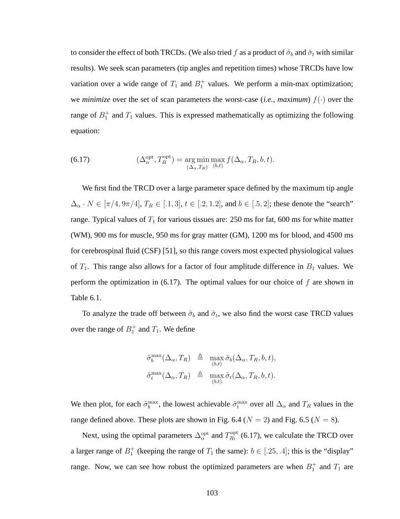
to consider the effect of both TRCDs. (We also triedf as a product ofσb andσt with similar

results). We seek scan parameters (tip angles and repetition times) whose TRCDs have low

variation over a wide range ofT1 andB+1 values. We perform a min-max optimization;

we minimize over the set of scan parameters the worst-case (i.e., maximum) f(·) over the

range ofB+1 andT1 values. This is expressed mathematically as optimizing thefollowing

equation:

(∆optα , T opt

R ) = arg min(∆α,TR)

max(b,t)

f(∆α, TR, b, t).(6.17)

We first find the TRCD over a large parameter space defined by the maximum tip angle

∆α · N ∈ [π/4, 9π/4], TR ∈ [.1, 3], t ∈ [.2, 1.2], andb ∈ [.5, 2]; these denote the “search”

range. Typical values ofT1 for various tissues are: 250 ms for fat, 600 ms for white matter

(WM), 900 ms for muscle, 950 ms for gray matter (GM), 1200 ms forblood, and 4500 ms

for cerebrospinal fluid (CSF) [51], so this range covers most expected physiological values

of T1. This range also allows for a factor of four amplitude difference inB1 values. We

perform the optimization in (6.17). The optimal values for our choice off are shown in

Table 6.1.

To analyze the trade off betweenσb andσt, we also find the worst case TRCD values

over the range ofB+1 andT1. We define

σmaxb (∆α, TR) , max

(b,t)σb(∆α, TR, b, t),

σmaxt (∆α, TR) , max

(b,t)σt(∆α, TR, b, t).

We then plot, for eachσmaxb , the lowest achievableσmax

t over all∆α andTR values in the

range defined above. These plots are shown in Fig. 6.4 (N = 2) and Fig. 6.5 (N = 8).

Next, using the optimal parameters∆optα andT opt

Ri (6.17), we calculate the TRCD over

a larger range ofB+1 (keeping the range ofT1 the same):b ∈ [.25, .4]; this is the “display”

range. Now, we can see how robust the optimized parameters are whenB+1 andT1 are

103

outside the original search range. We plot, for eachB+1 value in the display range, the

maximumσ over theT1 search range on one set of graphs (e.g., σb in plot B andσt in plot

D); and also for eachT1 value in the display range, the maximumσ over theB+1 search

range on another set of graphs (e.g., σb in plot A andσt in plot C). The graphs are shown

in Fig. 6.1, Fig. 6.2, and Fig. 6.3.

Table 6.1: Optimized scan parameters based on (6.17)Model N ∆α or α ∆TR

or TR1 TR2

(radians) (sec) (sec)

SSI 2 1.1781 0.68 -SSI 4 1.3744 0.68 -SSI 8 0.8836 0.68 -AFI 2 1.0996 0.245 0.10AFI 4 1.3352 0.825 0.10AFI 8 1.0603 0.68 0.10BP 2 2.2776 0.825 -BP 4 0.9818 0.535 -BP 8 0.8836 0.825 -

6.4.4 Model Selection Discussion

In this analysis, we consider two main questions: 1) What is the trade off betweenσb

andσt? and 2) How robust are the optimal parameters found in (6.17)?

Fig. 6.4 and Fig. 6.5 show the trade off betweenσmaxb and σmax

t . Improved accuracy

in estimatingB+1 decreasesT1 accuracy. Therefore, in scan parameter optimization, a

function of both TRCDs is required. The SSI and AFI method havethe lowest achievable

worst case TRCD (the BP method is outside Fig. 6.4). Clearly, the SSI method has the best

performance forN = 2; both the AFI and SSI method perform well forN = 8, with the

AFI method having a slight advantage.

The optimal parameters robustness varies both on the methodand the number of scans

(see Figures (6.1), (6.2), and (6.3). TRCD, for all methods, is lowest whenT1 is small

(plots A and C), but is more robust to the value ofB+1 (plots B and D). This is especially

104

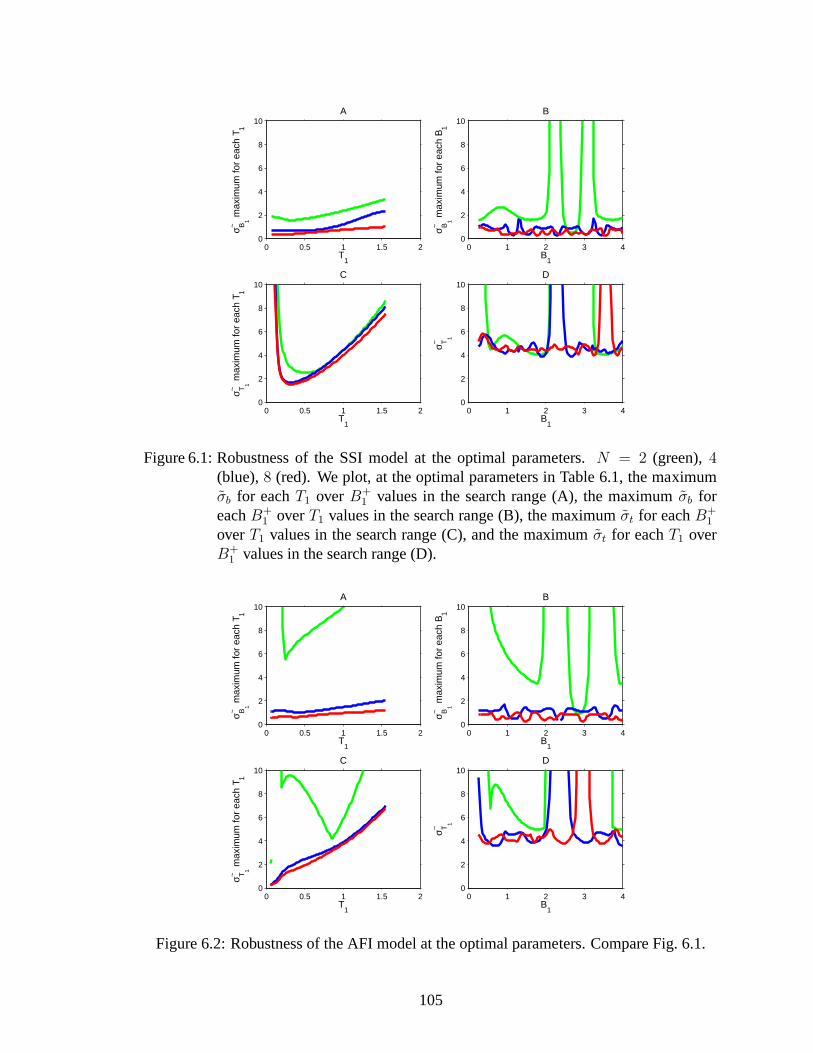
0 0.5 1 1.5 20

2

4

6

8

10

T1

σ B1

~ m

axim

um fo

r ea

ch T

1

A

0 1 2 3 40

2

4

6

8

10

B1

σ B1

~ m

axim

um fo

r ea

ch B

1

B

0 0.5 1 1.5 20

2

4

6

8

10

T1

σ T1

~ m

axim

um fo

r ea

ch T

1

C

0 1 2 3 40

2

4

6

8

10

B1

σ T1

~

D

Figure 6.1: Robustness of the SSI model at the optimal parameters. N = 2 (green),4(blue),8 (red). We plot, at the optimal parameters in Table 6.1, the maximumσb for eachT1 overB+

1 values in the search range (A), the maximumσb foreachB+

1 overT1 values in the search range (B), the maximumσt for eachB+1

overT1 values in the search range (C), and the maximumσt for eachT1 overB+

1 values in the search range (D).

0 0.5 1 1.5 20

2

4

6

8

10

T1

σ B1

~ m

axim

um fo

r ea

ch T

1

A

0 1 2 3 40

2

4

6

8

10

B1

σ B1

~ m

axim

um fo

r ea

ch B

1

B

0 0.5 1 1.5 20

2

4

6

8

10

T1

σ T1

~ m

axim

um fo

r ea

ch T

1

C

0 1 2 3 40

2

4

6

8

10

B1

σ T1

~

D

Figure 6.2: Robustness of the AFI model at the optimal parameters. Compare Fig. 6.1.

105

0 0.5 1 1.5 20

2

4

6

8

10

T1

σ B1

~ m

axim

um fo

r ea

ch T

1

A

0 1 2 3 40

2

4

6

8

10

B1

σ B1

~ m

axim

um fo

r ea

ch B

1

B

0.2 0.3 0.4 0.5 0.6 0.70

2

4

6

8

10

T1

σ T1

~ m

axim

um fo

r ea

ch T

1

C

0 0.2 0.4 0.6 0.8 10

2

4

6

8

10

B1

σ T1

~

D

Figure 6.3: Robustness of the BP model at the optimal parameters. Compare Fig. 6.1.

true for σt. For all methods,N = 4, 8 performs much better thanN = 2, especially for

the AFI method. Using four or eight scans, both the SSI and AFImethod are relatively

insensitive to specific values ofB+1 andT1 and are appropriate to use for joint estimation,

though SSI has the lowest TRCD values consistently. The BP method has relatively high

TRCD values, even whenN = 8, andσb is especially sensitive to the value ofB+1 , so this

method as implemented will have high variance for unbiasedB+1 estimation.

After analyzing the CRB for joint estimation ofB+1 andT1, the SSI method has both

the lowest worst case estimator variances and is the least sensitive toB+1 andT1 values.

The AFI method is also relatively insensitive toB+1 andT1 values, but, overall, has higher

estimator variances. The Brunner model, as modeled here, has poor performance, although

this may be improved by further optimizing other scan parameters in the model. Although

the results are not shown here, we also tried using the SSI model and varyingTR, but had

very poor results. We note that this optimization does neglect SAR constraints which may

be a problem when using a large tip angle and a short repetition time.

106

0 2 4 6 8 10 12 14 16 18 200

2

4

6

8

10

12

14

16

18

20

σT1~max

σ B1

~m

ax

SSIAFIBrunner

Figure 6.4: Minimum achievableσmaxb for a maximumσmax

t for two scans.

0 2 4 6 8 10 12 14 16 18 200

2

4

6

8

10

12

14

16

18

20

σT1~max

σ B1

~m

ax

SSIAFIBrunner

Figure 6.5: Minimum achievableσmaxb for a maximumσmax

t for eight scans.

107

6.4.5 CRB Extension: Joint estimation Versus Estimation WithOnly One Unknown

Variable

We now consider the “cost” of joint estimation,i.e., how much higher the CRB for

estimatingB+1 is for joint estimation ofB+

1 , T1 compared to estimatingB+1 with known

T1, given by(1/J11), as well as how much higher the CRB for estimationT1 is for joint

estimation ofB+1 /T1 compared to estimatingT1 with knownB+

1 , given by(1/J22). We

make graphs similar to Fig. 6.1 with three plots for each method, one each forN = 2,

N = 4, andN = 8. Each plot showsσ for joint estimation as a solid line andσ for

estimating one unknown variable as a dotted line. We use the same optimal values found

previously in computing the graphs. These graphs are shown in Fig. 6.6, Fig. 6.7, Fig. 6.8,

Fig. 6.9, Fig. 6.10, Fig. 6.11, Fig. 6.12, Fig. 6.13, and Fig.6.14.

0 0.5 1 1.5 20

2

4

6

8

10

T1

σ B1

~ m

axim

um fo

r ea

ch T

1

A

0 1 2 3 40

2

4

6

8

10

B1

σ B1

~ m

axim

um fo

r ea

ch B

1

B

0 0.5 1 1.5 20

2

4

6

8

10

T1

σ T1

~ m

axim

um fo

r ea

ch T

1

C

0 1 2 3 40

2

4

6

8

10

B1

σ T1

~

D

Figure 6.6: Cost of joint estimation for the SSI modelN = 2. Compare Fig. 6.1.σ forjoint estimation is shown with a solid line andσ for estimation of one unknownvariable is shown with a dotted line.

As expected,σ for joint estimation is higher thanσ for estimating just one unknown

variable in every case. The biggest difference is seen in theAFI method forN = 2.

108

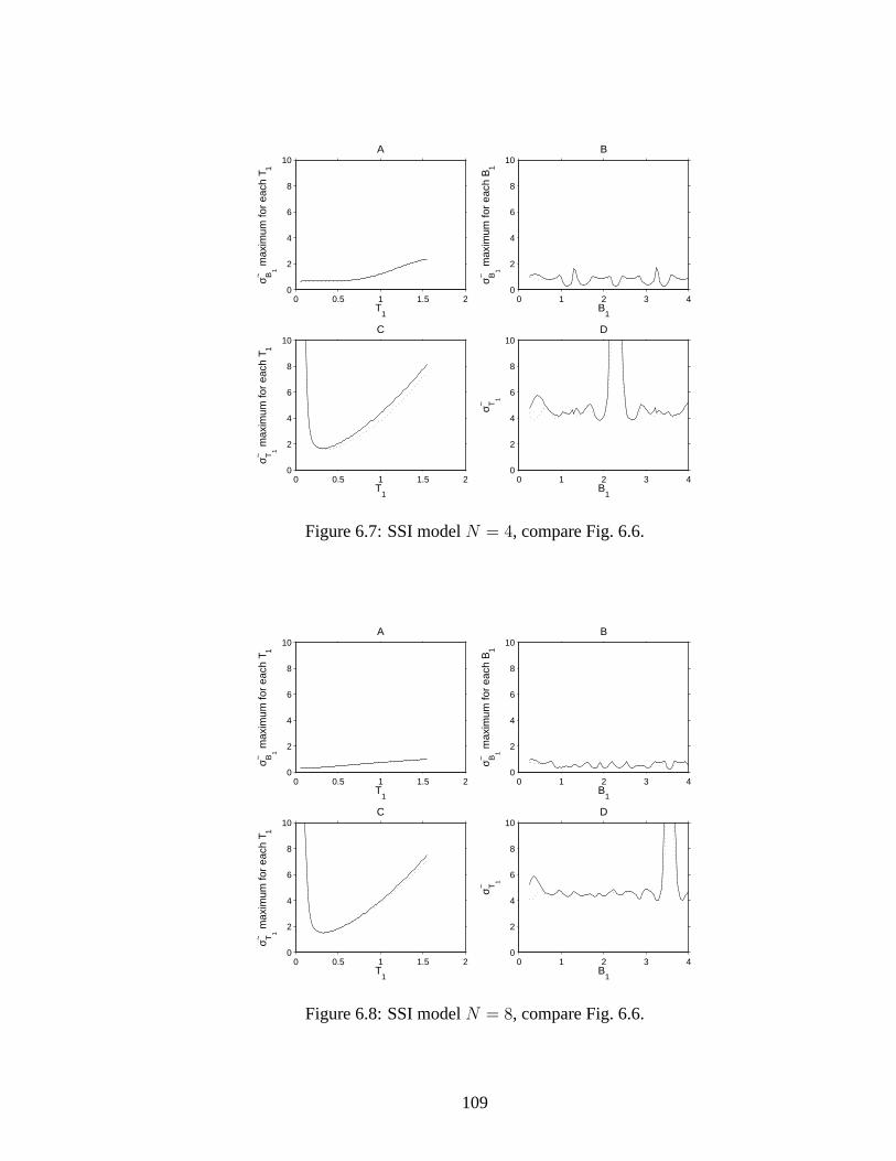
0 0.5 1 1.5 20

2

4

6

8

10

T1

σ B1

~ m

axim

um fo

r ea

ch T

1

A

0 1 2 3 40

2

4

6

8

10

B1

σ B1

~ m

axim

um fo

r ea

ch B

1

B

0 0.5 1 1.5 20

2

4

6

8

10

T1

σ T1

~ m

axim

um fo

r ea

ch T

1

C

0 1 2 3 40

2

4

6

8

10

B1

σ T1

~

D

Figure 6.7: SSI modelN = 4, compare Fig. 6.6.

0 0.5 1 1.5 20

2

4

6

8

10

T1

σ B1

~ m

axim

um fo

r ea

ch T

1

A

0 1 2 3 40

2

4

6

8

10

B1

σ B1

~ m

axim

um fo

r ea

ch B

1

B

0 0.5 1 1.5 20

2

4

6

8

10

T1

σ T1

~ m

axim

um fo

r ea

ch T

1

C

0 1 2 3 40

2

4

6

8

10

B1

σ T1

~

D

Figure 6.8: SSI modelN = 8, compare Fig. 6.6.

109

0 0.5 1 1.5 20

2

4

6

8

10

T1

σ B1

~ m

axim

um fo

r ea

ch T

1

A

0 1 2 3 40

2

4

6

8

10

B1

σ B1

~ m

axim

um fo

r ea

ch B

1

B

0 0.5 1 1.5 20

2

4

6

8

10

T1

σ T1

~ m

axim

um fo

r ea

ch T

1

C

0 1 2 3 40

2

4

6

8

10

B1

σ T1

~

D

Figure 6.9: AFI modelN = 2, compare Fig. 6.6.

0 0.5 1 1.5 20

2

4

6

8

10

T1

σ B1

~ m

axim

um fo

r ea

ch T

1

A

0 1 2 3 40

2

4

6

8

10

B1

σ B1

~ m

axim

um fo

r ea

ch B

1

B

0 0.5 1 1.5 20

2

4

6

8

10

T1

σ T1

~ m

axim

um fo

r ea

ch T

1

C

0 1 2 3 40

2

4

6

8

10

B1

σ T1

~

D


110

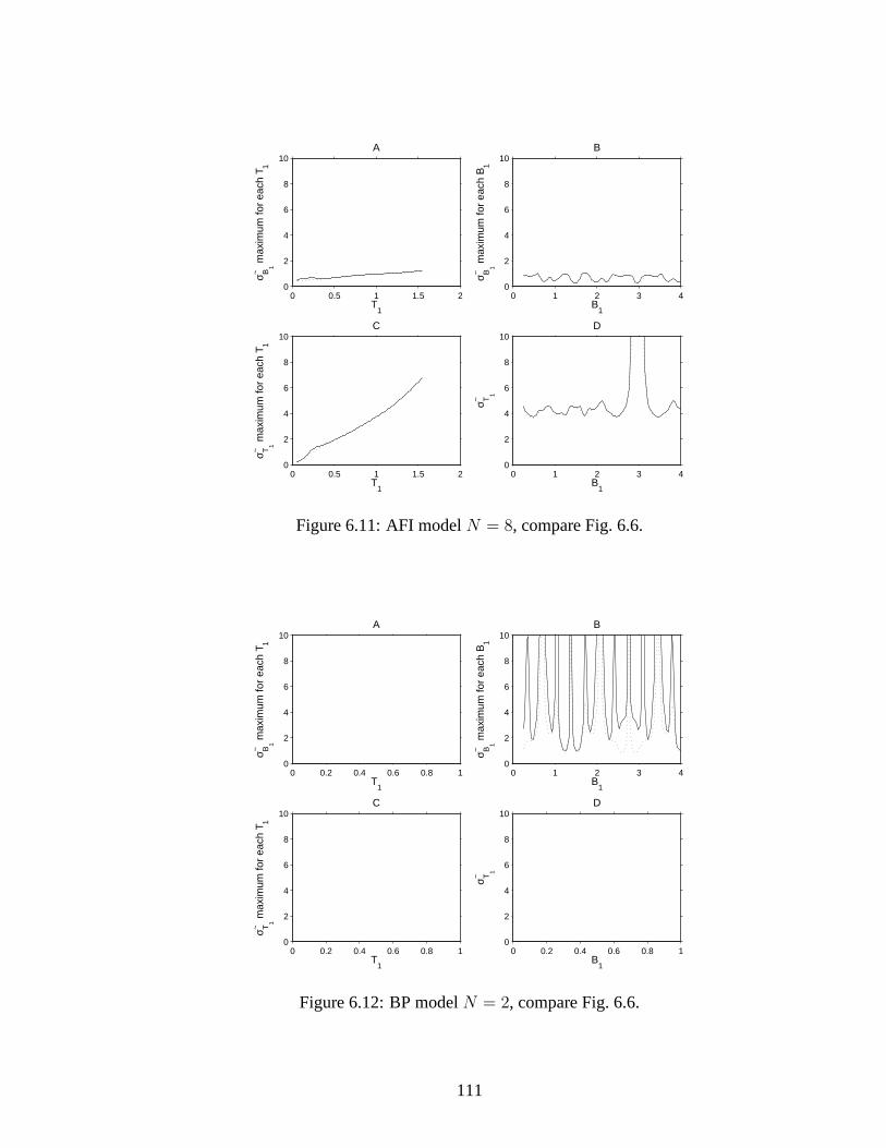
0 0.5 1 1.5 20

2

4

6

8

10

T1

σ B1

~ m

axim

um fo

r ea

ch T

1

A

0 1 2 3 40

2

4

6

8

10

B1

σ B1

~ m

axim

um fo

r ea

ch B

1

B

0 0.5 1 1.5 20

2

4

6

8

10

T1

σ T1

~ m

axim

um fo

r ea

ch T

1

C

0 1 2 3 40

2

4

6

8

10

B1

σ T1

~

D


0 0.2 0.4 0.6 0.8 10

2

4

6

8

10

T1

σ B1

~ m

axim

um fo

r ea

ch T

1

A

0 1 2 3 40

2

4

6

8

10

B1

σ B1

~ m

axim

um fo

r ea

ch B

1

B

0 0.2 0.4 0.6 0.8 10

2

4

6

8

10

T1

σ T1

~ m

axim

um fo

r ea

ch T

1

C

0 0.2 0.4 0.6 0.8 10

2

4

6

8

10

B1

σ T1

~

D

Figure 6.12: BP modelN = 2, compare Fig. 6.6.

111

0 0.2 0.4 0.6 0.8 10

2

4

6

8

10

T1

σ B1

~ m

axim

um fo

r ea

ch T

1

A

0 1 2 3 40

2

4

6

8

10

B1

σ B1

~ m

axim

um fo

r ea

ch B

1

B

0 0.2 0.4 0.6 0.8 10

2

4

6

8

10

T1

σ T1

~ m

axim

um fo

r ea

ch T

1

C

0 0.2 0.4 0.6 0.8 10

2

4

6

8

10

B1

σ T1

~

D

Figure 6.13: BP modelN = 4, compare Fig. 6.6. Some CRB values exceeded the axisrange.

0 0.5 1 1.5 20

2

4

6

8

10

T1

σ B1

~ m

axim

um fo

r ea

ch T

1

A

0 1 2 3 40

2

4

6

8

10

B1

σ B1

~ m

axim

um fo

r ea

ch B

1

B

0.2 0.3 0.4 0.5 0.6 0.70

2

4

6

8

10

T1

σ T1

~ m

axim

um fo

r ea

ch T

1

C

0 0.2 0.4 0.6 0.8 10

2

4

6

8

10

B1

σ T1

~

D

Figure 6.14: BP modelN = 8, compare Fig. 6.6.

112

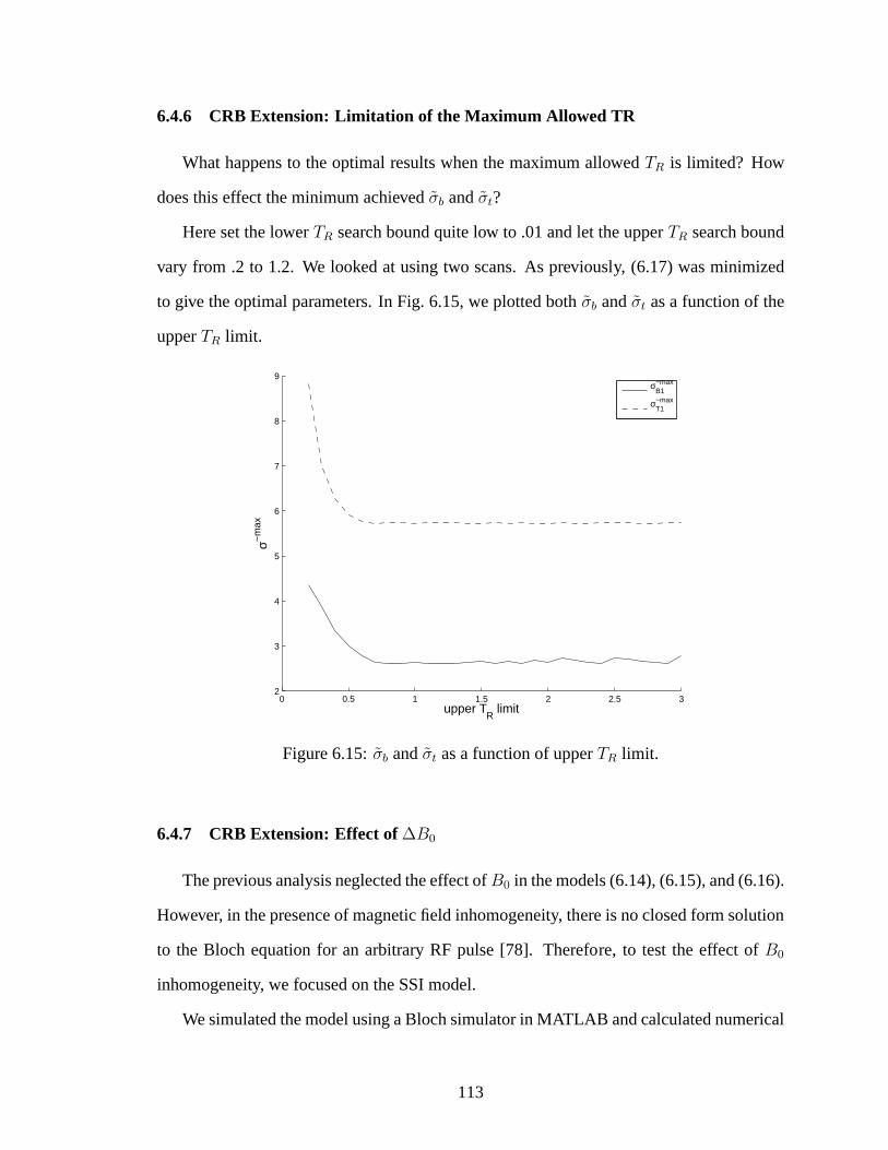
6.4.6 CRB Extension: Limitation of the Maximum Allowed TR

What happens to the optimal results when the maximum allowedTR is limited? How

does this effect the minimum achievedσb andσt?

Here set the lowerTR search bound quite low to .01 and let the upperTR search bound

vary from .2 to 1.2. We looked at using two scans. As previously, (6.17) was minimized

to give the optimal parameters. In Fig. 6.15, we plotted bothσb andσt as a function of the

upperTR limit.

0 0.5 1 1.5 2 2.5 32

3

4

5

6

7

8

9

upper TR

limit

σ~m

ax

σ

B1~max

σT1~max

Figure 6.15:σb andσt as a function of upperTR limit.

6.4.7 CRB Extension: Effect of∆B0

The previous analysis neglected the effect ofB0 in the models (6.14), (6.15), and (6.16).

However, in the presence of magnetic field inhomogeneity, there is no closed form solution

to the Bloch equation for an arbitrary RF pulse [78]. Therefore, to test the effect ofB0

inhomogeneity, we focused on the SSI model.

We simulated the model using a Bloch simulator in MATLAB and calculated numerical

113

derivatives from the equilibrium signal values. The CRB fromthe simulator for∆B0 = 0

matched the CRB when calculated with implicit or explicit differentiation as before. We

setB0 = 1.5 and let∆B0 = [0, 125, 250, 375, 500] Hz. We assumed a hard pulse (no slice

selection effects). For the SSI pulse, the number of pulses needed to achieve a relative error

err is given by:

nequ. =

[− T1

2TR

ln(err) − 1

2

],

where[·] is the ceiling operator. We seterr = 0.001 and repeated the pulse the larger of

5 or nequ. times. We originally did this analysis forN = 2, but the results are similar for

N > 2.

We used the optimal design parameters found in Table 6.1. Then, we calculated a

similar graph to Fig. 6.1. Here, in Fig. 6.16, each line corresponds to a different value of

∆B0. Clearly, we can see that the effect ofB0 inhomogeneity is very small and does not

overly effect the results of the previous analysis at the optimal parameters. Only when the

varianceσ becomes very large is the difference between the different amounts of magnetic

field inhomogeneity even seen.

6.4.8 CRB Extension: Possible Application to Multiple Coils

This analysis focuses only on a single coil, single voxel model. With multiple coils, we

theorize the possible effect on the effective combinedB+1 map would be a smallerB+

1 range

over the object. Therefore, we performed a similar analysisbut constrainedb ∈ [.81.2].

The optimal parameters using the smallerB+1 range are shown in Table 6.2. For the SSI

method, the optimal parameters are similar, but the optimalparameters are quite different

for the BP method.

The graphs similar to Fig. 6.1 are reproduced below in Fig. 6.17, Fig. 6.18, and Fig. 6.19.

The SSI model performs similarly, with slightly better results as does the AFI and we

114

0 0.5 1 1.5 2

x 106

0

2

4

6

8

10

T1

σ B1

~ m

axim

um fo

r ea

ch T

1

A

0 1 2 3 40

2

4

6

8

10

B1

σ B1

~ m

axim

um fo

r ea

ch B

1

B

0 0.5 1 1.5 2

x 106

0

2

4

6

8

10

T1

σ T1

~ m

axim

um fo

r ea

ch T

1

C

0 1 2 3 40

2

4

6

8

10

B1

σ T1

~

D

Figure 6.16: Magnetic field inhomogeneity effect on SSI model. N = 2, compare Fig. 6.1.Each line corresponds to a different level of magnetic field inhomogeneityfrom 0 to 500 Hz whenB0 = 1.5 T.

can see large improvements with the BP method.

115

0 0.5 1 1.5 20

2

4

6

8

10

T1

σ B1

~ m

axim

um fo

r ea

ch T

1

A

0 1 2 3 40

2

4

6

8

10

B1

σ B1

~ m

axim

um fo

r ea

ch B

1

B

0 0.5 1 1.5 20

2

4

6

8

10

T1

σ T1

~ m

axim

um fo

r ea

ch T

1

C

0 1 2 3 40

2

4

6

8

10

B1

σ T1

~

D

Figure 6.17: Application to multiple coils for the SSI model. N = 2 (solid line),4 (dottedline), 8 (dashed line). We plot, at the optimal parameters in Table 6.1, themaximumσb for eachT1 overB+

1 values in the search range (A), the maxi-mum σb for eachB+

1 overT1 values in the search range (B), the maximumσt

for eachB+1 overT1 values in the search range (C), and the maximumσt for

eachT1 overB+1 values in the search range (D).

0 0.5 1 1.5 20

2

4

6

8

10

T1

σ B1

~ m

axim

um fo

r ea

ch T

1

A

0 1 2 3 40

2

4

6

8

10

B1

σ B1

~ m

axim

um fo

r ea

ch B

1

B

0 0.5 1 1.5 20

2

4

6

8

10

T1

σ T1

~ m

axim

um fo

r ea

ch T

1

C

0 1 2 3 40

2

4

6

8

10

B1

σ T1

~

D

Figure 6.18: Application to multiple coils for the AFI model. Compare Fig. 6.1.

116

Table 6.2: Optimized scan parameters based on (6.17) with small B+1 range

Model N ∆α or α ∆TRor TR1 TR2

(radians) (sec) (sec)

SSI 2 1.9006 0.82 -SSI 4 1.3587 0.61 -SSI 8 0.8836 0.52 -AFI 2 0.6441 0.67 0.10AFI 4 1.0132 0.61 0.10AFI 8 0.8522 0.64 0.10BP 2 0.3927 0.825 -BP 4 0.1963 0.535 -BP 8 0.0982 0.825 -

0 0.5 1 1.5 20

2

4

6

8

10

T1

σ B1

~ m

axim

um fo

r ea

ch T

1

A

0 0.5 1 1.5 20

2

4

6

8

10

B1

σ B1

~ m

axim

um fo

r ea

ch B

1

B

0 0.5 1 1.50

2

4

6

8

10

T1

σ T1

~ m

axim

um fo

r ea

ch T

1

C

0.2 0.4 0.6 0.8 1 1.20

2

4

6

8

10

B1

σ T1

~

D

Figure 6.19: Application to multiple coils for the BP model.Compare Fig. 6.1.

117

6.5 JointB+

1,T1 estimation: Theory

6.5.1 Signal model for multiple coils, multiple tip angles/coil combinations and/or

multiple TRs

Suppose there areK coils. We takeM measurements by transmitting with different

coil combinations and receiving from a common coil. (This method could be generalized

to use multiple receive coils.) For each measurement, one ormore coil(s) are driven si-

multaneously by the same RF signalb1(t) with possibly different known amplitude scaling

factorsαmk, wherek denotes the coil number,m = 1, . . . ,M denotes the measurement

number, andα is aM × K array containing the scaling factorsαmk. For the problem to

be tractable, we require thatM > K + 2. The complex coil patterns sum together due

to linearity to make the total transmittedB+1 field. This general model encompasses the

conventional model if we letK = 1,M = 2, and

α =

1

2

.

We model the resultingM reconstructed images as follows:

(6.18) yjm = fjF

(K∑

k=1

αmkzjk, Tj,∆B0j ,TR m

)+ εjm,

for m = 1, . . . ,M andj = 1, . . . , N , wherefj denotes the underlying object transverse

magnetization in thejth voxel (multiplied by the sensitivity of the receive coil)andεjm

denotes zero-mean complex gaussian noise.TR m is the repetition time of the pulse se-

quence.∆B0 is the offset in theB0 field; we assume this is known (see [44], for example).

T is theT1 map over the object.

TheB+1 map, constrained to be real in the conventional model, is actually a complex

quantity.zjk denotes the unknown complexB+1 map that relates RF amplitude to tip angle

118

and phase at thejth voxel for thekth coil. When multiple coils are driven by the same signal

b1(t) (with possibly different amplitudes), then the fields from those coils will superimpose

and the complex coil patterns will add by linearity, hence the sum overk in (6.18). If

the units of the amplitudesαmk are gauss, then the units ofzjk will be radians per gauss.

More typically, the units ofαmk are arbitrary, and all that is known is their relative values.

In this casezjk will have units such that the product ofαmk andzjk has units of radians.

This should suffice for RF pulse design. We would like to use asfew coil combinations as

possible, while still being able to estimate each coil pattern zjk accurately.

The functionF in (6.18) is a generalization of the SSI method that inherently incorpo-

rates slice selection effects. The functionF is explained further in Section 6.5.3. We will

not show explicitlyF ’s dependence on∆B0 andTR because these are known constants

with respect to this model.

The model (6.18) expands the one used in [41,42] (whereTR was infinity) and includes

both slice selection effects and linear transceive coil combinations. By jointly estimating

T1 andB+1 , the SSI signal model allows for shorterTR values to be used

RecentB1 mapping methods [10, 90] have introduced linear combinations of transmit

coils. These methods have the advantage of using much smaller tip angles while still col-

lecting enough signal to produce accurate results. The proposed method accommodates this

matrix transmit technique with a comprehensive measurement model that also can include

slice selection effects and accounts for the noise factors that are often ignored by existing

methods.

The goal is to estimate eachB+1 map zk , (z1k, . . . , zNk) and theT1 map T ,

(T1, . . . , TN) from the reconstructed imagesyjm. The underlying magnetizationf ,

(f1, . . . , fN) is also unknown but is a nuisance parameter. We would like theestimator to

work robustly even in image regions wherefj is small.

If fj were allowed to be complex, then the model above would be non-identifiable

because we could add phase tof and subtract the same phase from eachzk andE[yjkl]

119

would remain unchanged. We take the approach of constraining f to be real. This reduces

the ambiguity to a sign change off and a correspondingπ phase shift in each phase map.

This does have the disadvantage of assigning any object phase (fromδB0, for example) into

the phase of theB+1 maps, which may influence the smoothness of theB+

1 maps. Another

solution that also makes the problem identifiable assumes that the first coil’s phase map is

zero and then all the other phase map values would be relativephases, in which casef can

be complex.

We also note a single surface coil for receive will suffice, even when multiple transmit

coils are used. In this case,f will be a product of the spin density and the receive coil

sensitivity pattern andz will include a constant (overk) phase offset from the receive coil.

6.5.2 Regularized estimator

We propose to jointly estimate theB+1 mapsz = (z1, . . . ,zK), theT1 mapT , and the

objectf by finding minimizers of the following penalized least squares cost function:

(z, T , f) = arg minz,T ,f

Ψ(z,T ,f),

Ψ(z,T ,f ,TR ) = L(z,T ,f) + βzR(z) + βTR(T ) + βfR(f),(6.19)

where

L(z,T ,f) =N∑

j=1

M∑

m=1

1

2


(K∑

k=1

αmkzjk,T

)∣∣∣∣∣

2

(6.20)

and

R(z) =K∑

k=1

R(zk),(6.21)

whereR(zk) is regularizing roughness penalty function for thekth B+1 map. Eachβ is a

regularization parameter that controls the smoothness of the estimate. Because one may

120

desire different amounts of smoothing for each map, we labeleach parameter:βz, βT , βf .

However, each parameter is user-chosen based on the desiredamount of smoothing (ex-

plained in Appendix L) and is not a function of any variable. Spatial resolution analysis

aids in selection of eachβ.

We use quadratic regularization for the mapszk becauseB+1 maps are expected be

spatially smooth, although edge-preserving regularization could be used if needed. We

note that although there seems to be plausible reasons why a particularB+1 map might

not be smooth, in the literature,B+1 maps are always very smooth. This is true, even in

cases such as cancer where there is a large deviation from thenormal brain, presumably

because the main cause of RF inhomogeneity, even in abnormalsubjects, is due to air/water

susceptibility as the RF waves propagate [13]. We use edge-preserving regularization for

both T1 (and, if desired,f ), because they contain detailed structural information, along

with a relatively smallβ to preserve detail.

There is no analytical solution for the minimizer ofΨ(z,T ,f) over all parameters, so

iterative methods are required.

Minimization with respect toz andT is nontrivial due to the non-linearity ofF . Pos-

sible minimization approaches include quadratic majorizer principles (see Section 3.6.1),

or variable projection (see Section 5.2.3), or generalizedoptimization methods. We choose

to use the gradient descent method specified below. Derivatives for the gradient descent

method are described in detail in Appendix I and Appendix J.

We use a preconditioned gradient descent method. There are many possibilities for

updating all the variables. We can use either a simultaneousupdate for all variables or a

block alternating minimization approach. With a simultaneous update for all variables, let

v =

[z T f

], and then

v(n+1) = v(n) + αnd(n),(6.22)

121

whered is the search direction given by the gradient of the cost function with respect to

each variable, letting the preconditioning matrix equal the identity matrix in this paper (see

Section I for the derivatives).

Ideally, by an exact line searchαn = arg minα Ψ(v(n) + α d(n)

). In practice, we

chooseα using Newton’s method as follows [30]:

Ψ(α) = Ψ(v(n) + αd(n)

)

Ψ(α) = ∇Ψ(v(n) + αd(n)

)d(n)

Ψ(α) =(d(n)

)′ ∇2 Ψ(v(n) + αd(n)

)d(n)

≈ 1/ǫ(Ψ(α+ ǫ) − Ψ(α)

),

and finally, we let

αn = −Ψ(0)

Ψ(0)

≈∣∣−∇Ψ

(v(n)

)d(n)

∣∣∣∣1

ǫ(∇Ψ (v(n) + ǫd(n)) d(n) −∇Ψ (v(n)) d(n))

∣∣ .(6.23)

This still requires care in choosingǫ. Here, we let

ǫ =max |v|max |d| ∗ .01,

where .01 was chosen empirically. Then, to force monotonicity, following [71], we set

α = α/2 until Ψ(v(n) + αnd(n)

)≤ Ψ

(v(n)

).

We note that for a given estimatez(n) of z and T (n) of T at thenth iteration, the

minimizer ofΨ with respect tof , assuming no regularization off , is found analytically to

be:

(6.24) fj

(n)=

∑Mm=1 real

y∗jmF (x

(n)jm, T

(n)j )

∑Mm=1

∣∣∣F (x(n)jm, T

(n)j )∣∣∣2 ,

122

where we define the compositeB+1 mapsxm as follows:

(6.25) xjm ,

K∑

k=1

αmkzjk.

In this thesis, we choose to use an alternating minimizationapproach in each step, al-

ternating which variable we minimize inv as in (6.22) while holding the other variables

constant. We use this method because we do not regularize theobject and also because

the step size in PGD minimization scales appropriately for each variable. Simultaneous

gradient descent appeared to converge slower; however, we anticipate that with a suitable

diagonal preconditioner, this method would also be acceptable. In Section 6.6.1 and Sec-

tion 6.6.2, we used a set number of iterations that gave good qualitative results; ideally, we

would use stopping rules based on, for example, percent change in the iterative estimates.

We note thatT1 has a constraint thatT > 0. We modify the alternating PGD mini-

mization to perform constrained minimization by performing a variable transformation as

explained in Appendix M.

The cost functionΨ is non-convex, so the alternating minimization algorithm described

above will descend from the initial estimates to a local minimum [63]. Thus it is essential

to choose reasonable initial estimates. See Appendix K for details.

Regularized methods have the benefit of being able to choose avalue forβ based on

quantitative analysis. In Appendix L, we analyze the spatial resolution of the regularized

estimator (6.19). This analysis leads to a modified penalty function that achieves more

uniform spatial resolution in regions with a constantfj. We choose a value for eachβ

based on the desired FWHM of regularizer smoothing.

6.5.3 F and Slice Selection Effects

In (6.18),F is a function that can incorporate both the type of pulse sequence being

used as well as slice selection effects by using a Bloch equation simulator.

123

After considering an appropriate coordinate rotation, we can express the functionF by

the following equation:

(6.26) F (z, t) = eı∠z H(|z| , t).

TabulatingF would require storing a look-up table with a complex input, while H has a

real input and we can store a lower dimensional table.H can be complex, depending on

the input RF pulse We conjecture that most symmetric RF pulses will have a realH; this

model is general enough to include other pulses, including non-symmetric ones. BothH

andF are potentially complex. Therefore, we tabulateH and use (6.26) in our estimation

algorithm. During our Bloch simulation, we can also varyT1 values andB0 offset values to

create a more accurate table that incorporates a larger number of effects, albeit with longer

computation time.

Assuming no slice selection effects (i.e., the (unachievable) infinite sinc pulse is used,

or 3D imaging) and noB0 offset, we use the SSI model forF in this paper [16] where

HSSIi (φ, t) =

(1 − e−γi) sin(φi)

1 − e−γi cos(φi),(6.27)

whereγ = TR /t.

In the case of slice selection effects orB0 offsets (∆B0), we tabulateH by evaluating

the Bloch equation using a RF pulse and varying its amplitude; i.e., we use

(6.28) b1(υ) =θ

γ∫ Υ

0p(s)ds

p(υ),

whereΥ is the pulse length andp(υ) is the RF pulse shape and we vary the amplitudeθ

T1, and theB0 offset to create the three-dimensional table. In the case ofnon-selective

excitation, or in the small-tip angle regime with exactly onresonance excitation,θ would

be the excitation tip angle times theB+1 map. The tableH is calculated once for each RF

124

pulse: for convenience, we normalizeH to a maximum value of 1.

In future work, we hope to investigate other common pulses such as those ((B.3),(B.4))

in Appendix B.

We note that one could use a different excitation pulse for each measurement, in which

caseF would beFm. For simplicity, we assume the same RF pulse is used for each mea-

surement and suppress the subscriptm. We let the subscriptR denote the real part andI

denote the imaginary part of the quantity. For example, letFR denote the real part ofF and

let FI denote the imaginary part ofF so

F = FR + iFI.

Fig. 6.20, Fig. 6.21, and Fig. 6.22 each show a graph ofHR(θ,T ) keeping eitherT or

θ constant for the idealized pulse. The (null) imaginary partis not shown for the example

symmetric pulses. Fig. 6.23 shows the derivative ofHR(θ,T ) with respect toθ. Fig. 6.24

and Fig. 6.25 show the derivative ofHR(θ,T ) with respect toT .

6.6 JointB+

1,T1 Experiments

6.6.1 Simulations

To evaluate the regularizedB+1 andT1 map estimation method described above, we

performed a simulation study using synthetic true maps shown in Fig. 6.26. For the object

magnitudefj andT1, we used a simulated normal brain anatomical model with eachvoxel

classified into one of 11 different classes [4, 5] ForT1 truth, we generate an image using

the classified model and typicalT1 values for each class type. Forfj truth, we generated a

proton density image weighted byT ∗2 , again using the typical PD andT ∗

2 values for each

class. To use smaller images for truth, we resized these images using bicubic interpolation

and anti-aliasing. TheB+1 maps were simulated based on equations for a magnetic field in

a circular current loop [49,129].

125

−10 −5 0 5 10−1

−0.5

0

0.5

1Fr versus tips (radians) for T1=.01

−10 −5 0 5 10−0.8

−0.6

−0.4

−0.2

0

0.2

0.4

0.6Fr versus tips (radians) for T1=.96

−10 −5 0 5 10−0.5

0

0.5Fr versus tips (radians) for T1=1.96

−10 −5 0 5 10−0.4

−0.2

0

0.2

0.4Fr versus tips (radians) for T1=2.96

Figure 6.20: Graph ofHR(θ,T ) for an idealized infinite sinc pulse holdingT1 constant. Welet T1 equal

[0.01 0.96 1.96 2.96

]and varyθ along the horizontal axis.

126

0 1 2 30.225

0.23

0.235

0.24

0.245

0.25

0.255

0.26F2r versus T1 for tips = 15 deg

0 1 2 3

0.35

0.4

0.45


0 1 2 3

0.4

0.5

0.6

0.7


0 1 2 30.2

0.4

0.6

0.8

1F2r versus T1 for tips = 90 deg

Figure 6.21: Graph ofHR(θ,T ) for an idealized infinite sinc pulse holdingθ constant. Welet θ equal

[15 30 45 90

]and varyT along the horizontal axis.

127

0 1 2 30

0.1

0.2

0.3

0.4


0 1 2 3−0.35

−0.3

−0.25

−0.2

−0.15

−0.1

−0.05


0 1 2 3−1

−0.8

−0.6

−0.4

−0.2


0 1 2 3−0.9

−0.8

−0.7

−0.6

−0.5

−0.4

−0.3

−0.2F2r versus T1 for tips = 300 deg

Figure 6.22: Graph ofHR(θ,T ) for an idealized infinite sinc pulse holdingT1 constant.We letθ equal

[150 200 250 300

]and varyT along the horizontal axis.

128

−10 −5 0 5 10−1

−0.5

0

0.5

1F2r db1 versus tips for T1 = .01

−10 −5 0 5 10−0.4

−0.2

0

0.2

0.4

0.6

0.8

1F2r db1 versus tips for T1 = .96

−10 −5 0 5 10−0.4

−0.2

0

0.2

0.4

0.6

0.8

1F2r db1 versus tips for T1 = 1.96

−10 −5 0 5 10−0.2

0

0.2

0.4

0.6

0.8

1

1.2F2r db1 versus tips for T1 = 2.96

Figure 6.23: Graph of the first derivative ofHR(θ,T ) with respect toθ for an idealizedinfinite sinc pulse. We holdT1 constant

[0.01 0.96 1.96 2.96

]and varyθ

along the horizontal axis.

129

0 1 2 3−0.012

−0.01

−0.008

−0.006

−0.004

−0.002

0F2r dt1 versus T1 for tips = 15 deg

0 1 2 3−0.08

−0.06

−0.04

−0.02


0 1 2 3−0.25

−0.2

−0.15

−0.1

−0.05


0 1 2 3−0.8

−0.6

−0.4

−0.2


Figure 6.24: Graph of the first derivative ofHR(θ,T ) with respect toT for an idealizedinfinite sinc pulse. We holdθ constant

[15 30 45 90

]and varyT along

the horizontal axis.

130

0 1 2 3−0.7

−0.6

−0.5

−0.4

−0.3

−0.2

−0.1


0 1 2 30

0.1

0.2

0.3

0.4

0.5F2r dt1 versus T1 for tips = 200 deg

0 1 2 30

0.2

0.4

0.6

0.8


0 1 2 30

0.1

0.2

0.3

0.4

0.5F2r dt1 versus T1 for tips = 300 deg

Figure 6.25: Graph of the first derivative ofHR(θ,T ) with respect toT for an idealizedinfinite sinc pulse. We holdθ constant

[150 200 250 300

]and varyT

along the horizontal axis.

131

Magnitude simulated true B1 map

1 73

1

87

0.2

0.4

0.6

0.8

1

1.2

1.4

Angle of simulated true B1 map

1 73

1

87

−3

−2

−1

0

1

2

3

Simulated true T1 map

1 73

1

87 0

0.5

1

1.5

2

2.5

Simulated true object

1 73

1

87 0

0.2

0.4

0.6

0.8

Figure 6.26: True simulated maps.

132

We simulated noisy reconstructed images forK = 4 different transmit coils using the

model (6.18). We assumed an ideal sinc RF pulse. For our scaling matrixα, we used both

“one-coil-at-a-time” (OAAT) (i.e., forM = 3K

αOAAT = α ·

IK

2 · IK3 · IK

,(6.29)

whereIk is aK ×K identity matrix) and “leave-one-coil-out” (LOO) (i.e., forM = 3K

αLOO =

α1K − αIK

2α · 1K − 2 · IK3α · 1K − 3 · IK

,(6.30)

where1K is aK ×K matrix of ones). There are many possible choices forα but we focus

on these two possible matrices to illustrate the method. Both matrices are well-conditioned

(κ (αOAAT) = 1 andκ (αLOO) = 3). In [91], these two different coil combinations are

analyzed with respect to the AFI model, but the results applyto all types ofB+1 mapping.

They found that the LOO method has significantly better map quality than the OAAT,

which has strong noise. LOO balances the trade off between noise, especially at low flip

angles, and the complementarity of multiple coil maps and can reduce mapping error by an

order of magnitude.

We added complex gaussian noise such that the SNR,10 log10(‖y‖/‖y − E[y]‖), was

either about 60 or 30 dB. Some of these images are shown in Fig.6.27.

We used either 12 or 16 measurements. For 12 measurements, werepeated each coil

combination three times atα, 2α, and3α (see (6.29) and (6.30)), allowing us to use the

triple angle initialization explained in Appendix K. We also compared the method with

16 total measurements, which also included4α. We fixedTR = 0.68 s andα = 1.3744

based on the analysis in Section 6.4 for the SSI model withN = 4. We used 50 iterations

133

y_1

1 73

1

87

0.1

0.2

0.3

0.4

0.5

0.6

y_5

1 73

1

87

0.1

0.2

0.3

0.4

0.5

0.6

y_8

1 73

1

87

0.1

0.2

0.3

0.4

0.5

0.6

y_12

1 73

1

87

0.1

0.2

0.3

0.4

0.5

0.6

Figure 6.27: Simulated noisy images. For the 1st, 5th, 8th, and 12th measurements (cor-responding to the respective rows in (6.30)). We used 4 coilsand leave-one-coil-out with an SNR of 60 dB.

134

(alternating which variable to minimize) with 15 internal PGD iterations to show the full

extent of the estimator, although for cases of high SNR, thisis excessive. Masked NRMSE

(reported in Table 6.3) for the jointB+1 , T1 estimation is compared to estimating onlyB+

1

using the regularization estimation explained in Chapter V,referring to this estimator as

the “previous” estimate. That method ignoresT1 effects, as ifTR = ∞. We note that the

initial T1 estimate here is the conventionalT1 estimate for the SSI method described in

Section 6.2.2.

First, we compared at a high SNR of 60 dB the OAAT method (shownin Fig. 6.28,

Fig. 6.29, Fig. 6.30, and Fig. 6.31) and LOO method (shown in Fig. 6.32. Fig. 6.33,

Fig. 6.34, and Fig. 6.35.) We note, in regards to the SNR, somecurrentT1 mapping papers

report SNRs ranging from 100 - 200 dB in the brain [14] and start to see significant bias

at about 60 dB [16], though these methods use a much lower TR (TR < 10 ms). We used

only 12 measurements because both methods perform well, with the most notable error in

theT1 map in OAAT in Fig. 6.30. We still see some small drop-out in theT1 map for LOO

Fig. 6.34, though theT1 map is definitely improved.

We also compared these methods when used at a lower SNR of 30 dB. Here, the OAAT

method struggled with only 12 measurements (figures not shown), so we used 16 measure-

ments. Even at 16 measurements, the noise necessitated using the previous method with

a small number of iterations as the initial guess. The finalf (see Fig. 6.39) andT1 (see

Fig. 6.38) strongly underestimate the interior of the brainwhich causes some corruption of

theB+1 magnitude maps (see Fig. 6.36). Clearly, using LOO improves all estimates, shown

in Fig. 6.40, Fig. 6.41, Fig. 6.42, and Fig. 6.43. There is still some overestimation ofT1

along the skull, but overall the estimates perform well at the lower SNR and with only 12

measurements.

The LOO method works reasonably well at smaller SNRs (results for 20 dB shown in

Table 6.3, figures not shown).

Overall, the simulation results shows that the proposed method works well, especially

135

Initial est. |B1|

1 73

1

870.5

1

1.5

Previous est. |B1|

1 73

1

870.5

1

1.5

Final est. |B1|

1 73

1

870.5

1

1.5

True |B1|

1 73

1

870.5

1

1.5

Initial error

1 73

1

87

−0.1

0

0.1

Previous error

1 73

1

87

−0.1

0

0.1

Final est. error

1 73

1

87

−0.1

0

0.1

Figure 6.28: MagnitudeB+1 maps for OAAT at 60 dB with 12 measurements.|z|, 50 it-

erations with 15 internal PGD iterations, 12 measurements,4 coils, “one at atime”, SNR around 60 dB,B+

1 map regularization parameter is2−3, T1 mapregularization parameter is2−5. No object regularization.

136

Initial est. B1 phase

1 73

1

87−202

Previous est. B1 phase

1 73

1

87−202

Final est. B1 phase

1 73

1

87−202

True B1 phase

1 73

1

87−202

Initial error

1 73

1

87

−0.2

0

0.2

Previous error

1 73

1

87

−0.2

0

0.2

Final error

1 73

1

87

−0.2

0

0.2

Figure 6.29: PhaseB+1 maps for OAAT at 60 dB with 12 measurements. Compare

Fig. 6.28.

137

Initial T1 est.

1 73

1

87 0.5

1

1.5Final T1 est.

1 73

1

87 0.5

1

1.5

True T1

1 73

1

87 0.5

1

1.5Initial error

1 73

1

87 −0.1

0

0.1Final error

1 73

1

87 −0.1

0

0.1

Figure 6.30: T1 maps for OAAT at 60 dB with 12 measurements. Compare Fig. 6.28.

using the LOO method or when using a larger number of measurements. Areas closer

to the skull tend to have some bias, especially in OAAT methods, but theB+1 maps are

consistently accurate at lower TR values in comparison to the previous method.

We chose our values forα based on our analysis in Section 6.4. However, we wished

to see if that analysis, based on the CRB, translated to our final implementation of our

joint B+1 , T1 estimator. These preliminary results took the simulated true maps (with all

four coils) and generated simulated data (16 measurements with “leave-one-out”) with an

SNR of approximately 30 dB. The first set of results, summarized in Table 6.4, keptα

constant and varied TR. Each set of parameters was only estimated once, so the results are

not statistically significant; however, the variance in theNRMSE is not large for these maps

and we can try to extrapolate from the table’s trends. Similarly, the second set of results,

summarized in Table 6.5, kept TR constant and variedα (by keeping the “leave-one-out”

and fixing theα2∗j = 2α1∗j andα3∗j = 3α1∗j andα4∗j = 4α1∗j for j = 1, 2, 3, 4).

We see from Table 6.4, that using TR values around the “optimal” TR of .68 ms gave

the lowest error for theB+1 maps, though a wide range of TR values gave very goodB+

1

138

Initial Object est.

1 73

1

87 0.5

1

1.5

Previous Object est

1 73

1

87 0.5

1

1.5

Final Object est.

1 73

1

87 0.5

1

1.5

True Object

1 73

1

87 0.5

1

1.5

Initial error

1 73

1

87 −0.1

0

0.1

Previous err

1 73

1

87 −0.1

0

0.1

Final error

1 73

1

87 −0.1

0

0.1

Figure 6.31: f estimates for OAAT at 60 dB with 12 measurements. Compare Fig.6.28.

139

Initial est. |B1|

1 73

1

870.5

1

1.5

Previous est. |B1|

1 73

1

870.5

1

1.5

Final est. |B1|

1 73

1

870.5

1

1.5

True |B1|

1 73

1

870.5

1

1.5

Initial error

1 73

1

87

−0.1

0

0.1

Previous error

1 73

1

87

−0.1

0

0.1

Final est. error

1 73

1

87

−0.1

0

0.1

Figure 6.32: MagnitudeB+1 maps for LOO at 60 dB with 12 measurements.|z|, 50 iter-

ations with 15 internal PGD iterations, 12 measurements, 4 coils, “leave oneout”, SNR around 60 dB,B+


140


1 73

1

87−202


1 73

1

87−202

Final est. B1 phase

1 73

1

87−202

True B1 phase

1 73

1

87−202

Initial error

1 73

1

87

−0.2

0

0.2

Previous error

1 73

1

87

−0.2

0

0.2

Final error

1 73

1

87

−0.2

0

0.2

Figure 6.33: PhaseB+1 maps for LOO at 60 dB with 12 measurements. Compare Fig. 6.32.

141

Table 6.3: Masked NRMSE for simulated images for differentα, numbers of measurements, and SNRmagB+

1 ∠B+1 T1 f

Coil config SNR M prev init final prev init final init final prev init final

OAAT 60 12 0.28 0.12 0.02 0.17 0.20 0.16 0.36 0.11 0.41 0.13 0.03LOO 60 12 0.39 0.37 0.015 0.18 0.18 0.14 0.13 0.10 0.37 0.02 0.02

OAAT 30 12 0.29 0.74 0.72 0.18 0.54 0.22 0.59 0.66 0.43 0.30 0.25OAAT 30 16 0.23 0.51 0.20 0.18 0.27 0.23 0.91 0.44 0.45 0.43 0.19LOO 30 12 0.39 0.13 0.06 0.22 0.49 0.15 0.29 0.19 0.37 0.09 0.07LOO 20 12 0.39 0.18 0.11 0.29 0.39 0.19 0.44 0.35 0.36 0.15 0.14LOO 20 16 0.31 0.22 0.08 0.28 0.78 0.22 0.48 0.32 0.45 0.16 0.12

142

Initial T1 est.

1 73

1

87 0.5

1

1.5Final T1 est.

1 73

1

87 0.5

1

1.5

True T1

1 73

1

87 0.5

1

1.5Initial error

1 73

1

87 −0.1

0

0.1Final error

1 73

1

87 −0.1

0

0.1

Figure 6.34: T1 maps for LOO at 60 dB with 12 measurements. Compare Fig. 6.32.

map estimates. Estimates ofT1 were more variable and would require more data to be

conclusive, though a slightly longer TR seems to give betterresults. This greater variability

(and greater difficulty in measuringT1) is suggested by our previous analysis, especially in

Fig. 6.1 where higherT1 values are more difficult to estimate. We can clearly see thisin

Fig. 6.34 where the highT1 values at the center of the brain are underestimated. The high

error at very low TR is predicted by Fig. 6.15. From Table 6.5,we see that usingα values

around the “optimal”α of 1.3744 give the lowest errors for estimating all maps. Very large

or very smallα values cause a much greater error. Assuming aB+1 range around 1, small

α values do not cover a wide enough range of tips to successfully estimateB+1 andT1. The

initialization was important for this study and using the previous estimate ofB+1 only for

the initialization strongly improved results when a very small or very large values ofα was

chosen.

143

Initial Object est.

1 73

1

87 0.5

1

1.5

Previous Object est

1 73

1

87 0.5

1

1.5

Final Object est.

1 73

1

87 0.5

1

1.5

True Object

1 73

1

87 0.5

1

1.5

Initial error

1 73

1

87 −0.1

0

0.1

Previous err

1 73

1

87 −0.1

0

0.1

Final error

1 73

1

87 −0.1

0

0.1

Figure 6.35: f estimates for LOO at 60 dB with 12 measurements. Compare Fig. 6.32.

144

Initial est. |B1|

1 73

1

870.5

1

1.5

Previous est. |B1|

1 73

1

870.5

1

1.5

Final est. |B1|

1 73

1

870.5

1

1.5

True |B1|

1 73

1

870.5

1

1.5

Initial error

1 73

1

87

−0.1

0

0.1

Previous error

1 73

1

87

−0.1

0

0.1

Final est. error

1 73

1

87

−0.1

0

0.1

Figure 6.36: MagnitudeB+1 maps for OAAT at 30 dB with 16 measurements.|z|, 50 it-

erations with 15 internal PGD iterations, 16 measurements,4 coils, “one at atime”, SNR around 30 dB,B+


145


1 73

1

87−202


1 73

1

87−202

Final est. B1 phase

1 73

1

87−202

True B1 phase

1 73

1

87−202

Initial error

1 73

1

87

−0.2

0

0.2

Previous error

1 73

1

87

−0.2

0

0.2

Final error

1 73

1

87

−0.2

0

0.2

Figure 6.37: PhaseB+1 maps for OAAT at 30 dB with 16 measurements. Compare

Fig. 6.36.

146

Initial T1 est.

1 73

1

87 0.5

1

1.5Final T1 est.

1 73

1

87 0.5

1

1.5

True T1

1 73

1

87 0.5

1

1.5Initial error

1 73

1

87 −0.1

0

0.1Final error

1 73

1

87 −0.1

0

0.1

Figure 6.38: T1 maps for OAAT at 30 dB with 16 measurements. Compare Fig. 6.36.

Table 6.4: Changes in NRMS with a change of TR, 1 estimate, 4 coils, 16 measurements,30 iterations with 10 PGD iterations, SNR = 30 dB,α = 1.38 · [1234]

TR value |b| joint |b| previous ∠b joint ∠b previous T joint f joint f previous

0.001 0.38 1.30 0.57 0.42 0.91 0.88 1.070.010 0.14 1.24 0.37 0.42 0.78 0.65 1.160.016 0.04 1.20 0.17 0.42 0.70 0.59 1.250.031 0.03 1.12 0.15 0.42 0.57 0.38 1.420.046 0.02 1.05 0.17 0.42 0.48 0.28 1.530.061 0.03 0.99 0.15 0.42 0.45 0.25 1.580.076 0.03 0.93 0.17 0.38 0.40 0.21 1.590.100 0.03 0.77 0.16 0.31 0.35 0.18 1.530.160 0.04 0.68 0.16 0.19 0.29 0.14 1.230.3 0.04 0.52 0.16 0.17 0.19 0.09 0.730.5 0.06 0.41 0.16 0.23 0.25 0.14 0.430.7 0.02 0.32 0.17 0.22 0.12 0.05 0.380.9 0.04 0.26 0.18 0.25 0.16 0.07 0.361.1 0.06 0.22 0.16 0.21 0.24 0.10 0.351.3 0.03 0.18 0.17 0.24 0.14 0.05 0.341.5 0.03 0.16 0.14 0.24 0.19 0.06 0.341.7 0.04 0.14 0.19 0.24 0.29 0.08 0.33

147

Initial Object est.

1 73

1

87 0.5

1

1.5

Previous Object est

1 73

1

87 0.5

1

1.5

Final Object est.

1 73

1

87 0.5

1

1.5

True Object

1 73

1

87 0.5

1

1.5

Initial error

1 73

1

87 −0.1

0

0.1

Previous err

1 73

1

87 −0.1

0

0.1

Final error

1 73

1

87 −0.1

0

0.1

Figure 6.39: f estimates for OAAT at 30 dB with 16 measurements. Compare Fig.6.36.

148

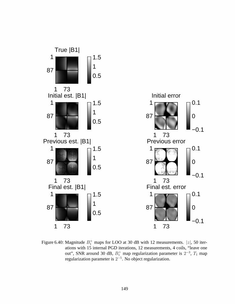
Initial est. |B1|

1 73

1

870.5

1

1.5

Previous est. |B1|

1 73

1

870.5

1

1.5

Final est. |B1|

1 73

1

870.5

1

1.5

True |B1|

1 73

1

870.5

1

1.5

Initial error

1 73

1

87

−0.1

0

0.1

Previous error

1 73

1

87

−0.1

0

0.1

Final est. error

1 73

1

87

−0.1

0

0.1

Figure 6.40: MagnitudeB+1 maps for LOO at 30 dB with 12 measurements.|z|, 50 iter-

ations with 15 internal PGD iterations, 12 measurements, 4 coils, “leave oneout”, SNR around 30 dB,B+


149


1 73

1

87−202


1 73

1

87−202

Final est. B1 phase

1 73

1

87−202

True B1 phase

1 73

1

87−202

Initial error

1 73

1

87

−0.2

0

0.2

Previous error

1 73

1

87

−0.2

0

0.2

Final error

1 73

1

87

−0.2

0

0.2

Figure 6.41: PhaseB+1 maps for LOO at 30 dB with 12 measurements. Compare Fig. 6.40.

150

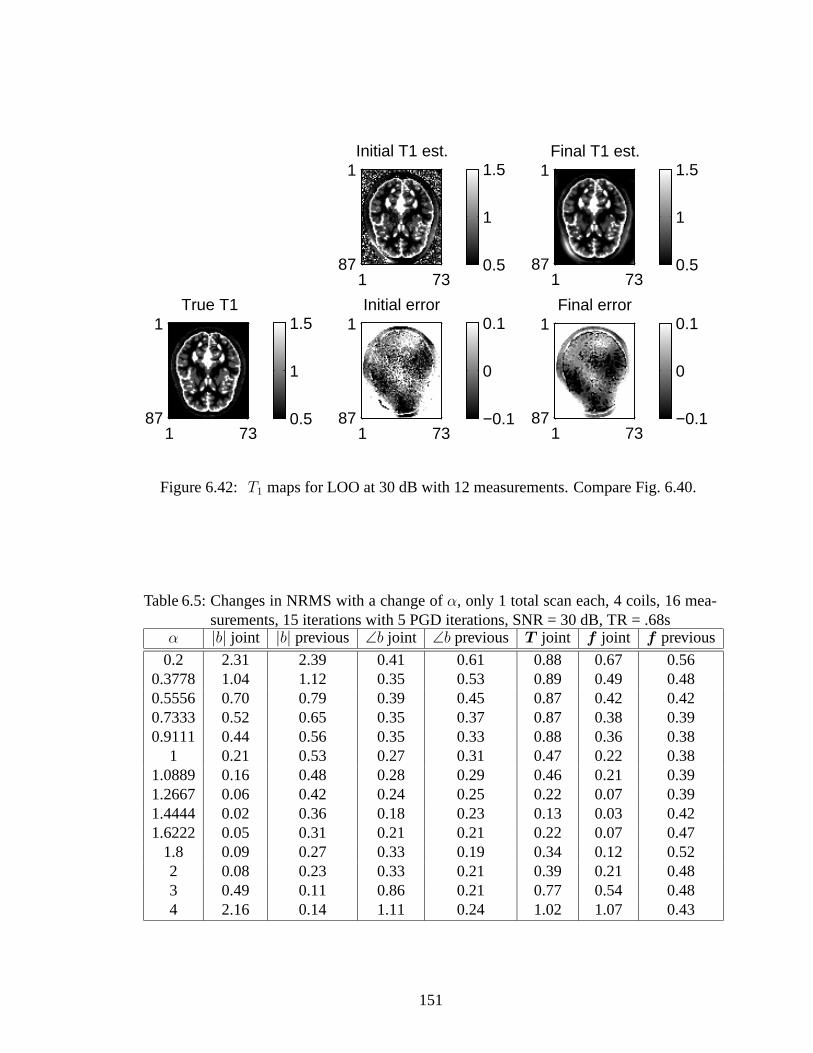
Initial T1 est.

1 73

1

87 0.5

1

1.5Final T1 est.

1 73

1

87 0.5

1

1.5

True T1

1 73

1

87 0.5

1

1.5Initial error

1 73

1

87 −0.1

0

0.1Final error

1 73

1

87 −0.1

0

0.1

Figure 6.42: T1 maps for LOO at 30 dB with 12 measurements. Compare Fig. 6.40.

Table 6.5: Changes in NRMS with a change ofα, only 1 total scan each, 4 coils, 16 mea-surements, 15 iterations with 5 PGD iterations, SNR = 30 dB, TR = .68s

α |b| joint |b| previous ∠b joint ∠b previous T joint f joint f previous

0.2 2.31 2.39 0.41 0.61 0.88 0.67 0.560.3778 1.04 1.12 0.35 0.53 0.89 0.49 0.480.5556 0.70 0.79 0.39 0.45 0.87 0.42 0.420.7333 0.52 0.65 0.35 0.37 0.87 0.38 0.390.9111 0.44 0.56 0.35 0.33 0.88 0.36 0.38

1 0.21 0.53 0.27 0.31 0.47 0.22 0.381.0889 0.16 0.48 0.28 0.29 0.46 0.21 0.391.2667 0.06 0.42 0.24 0.25 0.22 0.07 0.391.4444 0.02 0.36 0.18 0.23 0.13 0.03 0.421.6222 0.05 0.31 0.21 0.21 0.22 0.07 0.47

1.8 0.09 0.27 0.33 0.19 0.34 0.12 0.522 0.08 0.23 0.33 0.21 0.39 0.21 0.483 0.49 0.11 0.86 0.21 0.77 0.54 0.484 2.16 0.14 1.11 0.24 1.02 1.07 0.43

151

Initial Object est.

1 73

1

87 0.5

1

1.5

Previous Object est

1 73

1

87 0.5

1

1.5

Final Object est.

1 73

1

87 0.5

1

1.5

True Object

1 73

1

87 0.5

1

1.5

Initial error

1 73

1

87 −0.1

0

0.1

Previous err

1 73

1

87 −0.1

0

0.1

Final error

1 73

1

87 −0.1

0

0.1

Figure 6.43: f estimates for LOO at 30 dB with 12 measurements. Compare Fig. 6.40.

152

6.6.2 Phantom Real MR Images

Phantom real MR data was taken using a four coil setup. The phantom has a stated

trueT = 1s which we measured with an inversion recovery curve toT = 1.095s. For this

setup, varying TR was more reliable than varying the flip angle. Therefore, first one coil

was turned on and complex image measurements recorded over the field of view for a wide

range of TR values

20 40 60 80 100 120 160 200 300 500

1000 2000

ms. Next,

the other three coils were turned on separately and complex measurements recorded with

TR= 2000 ms. Samples of this data are shown in Fig. 6.44.

Coil 1, TR = 2 ms

1 64

1

64

5

10

15

20

25

Coil 2, TR = 2 ms

1 64

1

64

5

10

15

20

25

Coil 3, TR = 2 ms

1 64

1

64

2

4

6

8

Coil 4, TR = 2 ms

1 64

1

64

5

10

15

Figure 6.44: |y| transmitting individually for each of the four coils with TR= 2000 ms.

The initial procedure described in Appendix K. These initial estimates are shown in

153

Fig. 6.45.

Init Masked Magnitude B1 maps

1 64

1

64

0

1

Init Masked Phase B1 maps

1 64

1

64

−2

0

2

Uniform: 1.08294

Init T1 Map

1 64

1

64 0

0.5

1

Init Object

1 64

1

64

20

40

Figure 6.45: Initial phantom estimates.

Using these initial estimates and all the data, we ran the proposed jointB+1 , T1 estimator

with 30 iterations with 15 iterations of the preconditionedgradient descent method algo-

rithm using alternating minimization. We regularized theB+1 map withβ = 2−3 and also

regularized theT1 map with edge preserving regularization andβ = 2−6. We performed

no object regularization. The final regularized images are shown in Fig. 6.46. We also ran

the algorithm using no regularization to compare model fit with final unregularized images

shown in Fig. 6.47.

Using these initial values, we measured model fit. We compared the measured magni-

tude data and compared that to the expected magnitude value using these initial values and

also using a final estimate using our proposed algorithm withno regularization. For a few

select pixels, graphs of the actual and estimated data (boththe initial B1 estimate and also

the final regularized estimate) are shown in the graphs belowfrom Fig. 6.48 to Fig. 6.51.

We repeated this graphs assuming that bothT1 andf are roughly constant and showing our

calculated initialB+1 along the x-axis. These are shown in Fig. 6.52 to Fig. 6.56. Overall,

154

Init Masked Magnitude B1 maps

1 64

1

64

0

1

Init Masked Phase B1 maps

1 64

1

64

−2

0

2

Uniform: 1.08294

Init T1 Map

1 64

1

64 0

0.5

1

Init Object

1 64

1

64

20

40

Figure 6.46: Final phantom regularized estimates.

Masked Magnitude B1 maps

1 64

1

64

0

1

Masked Phase B1 maps

1 64

1

64

−2

0

2

T1 Map

1 64

1

64

1

1.5

2

Object

1 64

1

64

20

40

Figure 6.47: Final phantom unregularized estimate.

155

the fit is very good and shows improvement over the initial estimate, especially at very low

B+1 map values.

156

0 0.5 1 1.5 22

2.2

2.4

2.6

2.8

3

3.2

3.4

TR

SS

I mag

nitu

de d

ata

valu

es

Model fit with b1 = 5 deg, new method, nmrs = 2%

Measured magnitude dataExpected (regularized final)Expected (init)

Figure 6.48: Phantom model fit,θ = 5 degrees, whereθ = αb

We also ran a second phantom study. Our first phantom study only used one coil at

a time and is comparable to the “one-at-a-time” simulation studies. The second phantom

study used several coils at a time and is more comparable to the “leave-one-out” simulation

studies. Thus, we would expect better performance from the second phantom study.

In the second phantom study, all four coils were first turned on and data was taken

at TR =

[50 100 500 2000

]ms. Then, three of the four coils were turned on and

data was collected at the same TR values. This was repeated for each of the 4 three-coil

combinations. The same general procedure was performed above with slight modifications.

Again, the initialB+1 map was estimated by minimizing the cost, but here, we estimated

the (complex) composite coil map. First, we used the estimated composite coils map as

157

0 0.5 1 1.5 20

2

4

6

8

10

12

TR

SS

I mag

nitu

de d

ata

valu

es




158

0 0.5 1 1.5 20

5

10

15

20

25

TR

SS

I mag

nitu

de d

ata

valu

es




159

0 0.5 1 1.5 20

5

10

15

20

25

TR

SS

I mag

nitu

de d

ata

valu

es




160

0 10

0.5

1

1.5

2

2.5

3

B1

SS

I dat

a va

lues

Model fit with TR = 0.02, new method, nrms = 13%

Measured dataExpected (regularized final)Expected (init)

Figure 6.52: Phantom model fit with respect to b1, TR = 20 ms

161

0 10

0.5

1

1.5

2

2.5

3

3.5

4

4.5

5

B1

SS

I dat

a va

lues




162

0 10

1

2

3

4

5

6

7

B1

SS

I dat

a va

lues




163

0 10

1

2

3

4

5

6

7

8

9

10

B1

SS

I dat

a va

lues




164

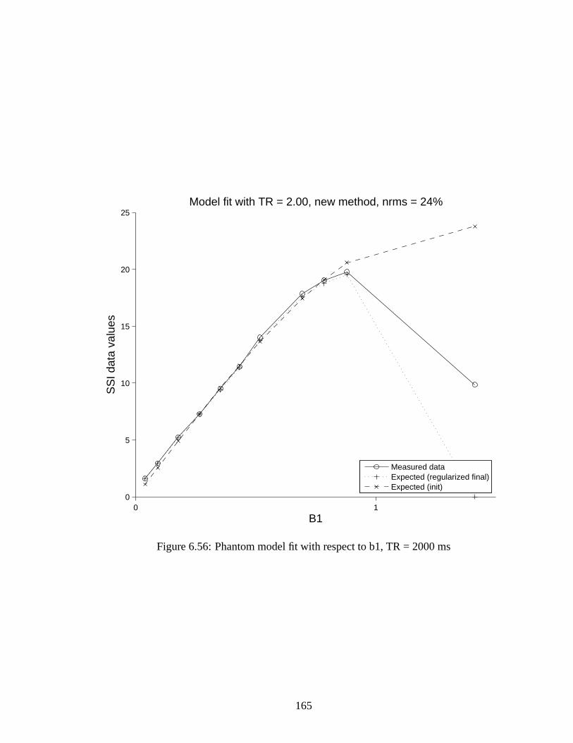
0 10

5

10

15

20

25

B1

SS

I dat

a va

lues




165

an initial estimate for our regularized estimator. These are shown in Fig. 6.58. Next, we

kept theT1 andf constant and estimated (via our regularized estimator) theindividual coil

maps to be our initial estimates for the algorithm. These areshown in Fig. 6.59. Finally,

we ran the regularized algorithm with these initial estimates. This final step only resulted

in small changes from the previous two-step procedure and ispossibly unnecessary. The

final estimate is shown in Fig. 6.60. The magnitude data with all coils turned on is shown

in Fig. 6.57. The initial estimates are shown in Fig. 6.59.

All Coils, TR = 50 ms

1 64

1

64

1

2

3

4

5All Coils, TR = 100 ms

1 64

1

64

1

2

3

4

5

6

7


1 64

1

64

2

4

6

8

10

12


1 64

1

64

5

10

15

Figure 6.57: Phantom magnitude data with all four coils turned on at four repetition times.

Using these values, we measured model fit. We compared the measured magnitude

data and compared that to the expected magnitude value usingthese initial values and also

using a final estimate using our proposed algorithm. For a fewselect pixels, graphs of

166


1 64

1

64 0

1


1 64

1

64−1

0

1

2

T1 Map

1 64

1

641

2

3

Object

1 64

1

64 0

10

20

30

Figure 6.58: Phantom: Regularized estimates for all coils turned on.


1 64

1

64

0

1


1 64

1

64

−2

0

2

T1 Map

1 64

1

641

2

3

Object

1 64

1

64 25.55

25.6

25.65

Figure 6.59: Phantom: estimate for individual coil maps.

167


1 64

1

64

0

1


1 64

1

64

−2

0

2

T1 Map

1 64

1

64 1

2

3

Object

1 64

1

64 0

20

40

Figure 6.60: Final regularized estimates using all data forthe second phantom experiment.Using 20 iterations with 5 internal PGD iterations. Regularization parameterfor B+

1 map is2−2 and for theT1 andf map is2−2.

168

the actual and estimated data (both the initial B1 estimate and also the final regularized

estimate) are shown in the graphs below from Fig. 6.61 to Fig.6.66. Overall, the fit is very

good and shows improvement over the initial estimate. From the images, we can still see

some possible residual model mismatch. The regularizationin the object appears to give

some residual error along the edge of theT1 map. However, theB+1 maps (the parameter

of interest) in Fig. 6.60 are smooth and match the data well, thus, achieving our goal.

1 2 3 4 5 6 7 8 9 10 11 12 13 14 15 16 17 18 19 200

0.5

1

1.5

2

2.5

3

3.5

Each measurement

SS

I mag

nitu

de d

ata

valu

es




This section shows the feasibility of estimating real MR data and also varying the repe-

tition time versus the tips angles for the SSI data. In the CRB analysis Section 6.4, keeping

a constant tip angle while varying TR had a much higher variance than the other methods.

Indeed, looking at Fig. 6.21 and Fig. 6.22, we can see thatH varies slowly withT1 (and re-

169

1 2 3 4 5 6 7 8 9 10 11 12 13 14 15 16 17 18 19 202.5

3

3.5

4

4.5

5

5.5

6

6.5

Each measurement

SS

I mag

nitu

de d

ata

valu

es




170

1 2 3 4 5 6 7 8 9 10 11 12 13 14 15 16 17 18 19 202

3

4

5

6

7

8

9

10

Each measurement

SS

I mag

nitu

de d

ata

valu

es




171

1 2 3 4 5 6 7 8 9 10 11 12 13 14 15 16 17 18 19 202

3

4

5

6

7

8

9

10

11

12

Each measurement

SS

I mag

nitu

de d

ata

valu

es




172

1 2 3 4 5 6 7 8 9 10 11 12 13 14 15 16 17 18 19 200

2

4

6

8

10

12

14

16

Each measurement

SS

I mag

nitu

de d

ata

valu

es




173

1 2 3 4 5 6 7 8 9 10 11 12 13 14 15 16 17 18 19 202

4

6

8

10

12

14

16

18

Each measurement

SS

I mag

nitu

de d

ata

valu

es




174

ciprocally, keepingT1 constant and varying TR), especially at low flip angles. Variation in

TR does not contain as much information as variation in tip angle (compare the differences

in the magnitude data in Fig. 6.57 where all measurements arequite similar to Fig. 6.27

where each measurement has greater variation depending onT1 values). Thus, we expect

that phantom MR studies while varying tip angle will have lower error and better final

estimates.

6.7 JointB+

1, T1 estimation: Discussion

We have described a new regularized method for jointB+1 andT1 mapping. Incorporat-

ing aT1 estimate allows for decreased required repetition times while still estimating the

B+1 magnitude and phase for multiple coils, especially for use in pulse sequence design.

TheB+1 maps interpolates smoothly in areas with low spin density with a user-chosen de-

sired FWHM. This method allows for an arbitrary selection of both tip angles and repetition

times, although careful selection of these aids the selection of an initial estimate.

This method is strongly based on our previous regularized method forB+1 mapping

Chapter V and is an extension that allows for shorter repetition values. While not investi-

gated in regards to joint estimation, this new method also allows for incorporation ofB0

inhomogeneity and correct slice profile.

The simulation results show that the NRMSE of the new jointB+1 estimates are less

than those of our previous estimator, due to incorporation of T1 effects.

In future work, we hope to investigate using different sliceprofiles and their subsequent

effects on the final estimates. We anticipate that addition of slice profile effects will show

a greater decrease in NRMSE compared to conventional estimators. We plan to implement

estimating phase map differences among the coils to circumvent possible object phase that

may contribute to less smoothness in the trueB+1 maps. We plan to further investigate the

optimal selection of tip angles and repetition times to minimize scan time while achieving a

low NRMSE. We plan to further investigate the spatial resolution, especially for the object,

175

and with multiple coils.

The model and estimators in this paper provide smooth, less noisy estimates that incor-

porateT1 effects and greater repetition times selection that allow for a possibly shorter scan

time and concurrentT1 estimation.

176

CHAPTER VII

Conclusion and Future Work

Due to the high field strength and temporal requirements in modern MRI, field maps

of the main fieldB0 and of the radio frequency fieldB1 are required for pulse design and

image correction. Many current estimators for these fields are heuristic and not based on

a comprehensive statistical model. This thesis proposed three new penalized-likelihood

estimators based on statistical models. The field map estimator uses multiple scans and

shows an empirical improvement with an improvement in RMSE over the conventional or

penalized-likelihood estimator with only two scans. TheB1 estimator uses a model that

accounts for a multiple coil design and includes slice-selection effects and allows for any

number of arbitrary tip angles, an improvement over the double angle conventional esti-

mator. The estimator additionally estimates both the magnitude and phase. The jointB+1 ,

T1 estimator accounts for a multiple coil design and allows forany number of arbitrary tip

angles and repetition times while estimating the magnitudeand phase for each coil and aT1

map. Simulation and MRI studies show the reduced noise and (for the simulation) reduced

RMSE when using each new PL estimator over the conventional estimator. Using PL esti-

mators and a statistical model yields better results than just using conventional estimators.

These estimators make smoother, less noisy estimates forB0 andB1 andT1 maps for use

in pulse design and image correction.

Ultimately, each of these methods is a tool that can only helpanswer the true question of

177

mapping: the best use of scan time to create the most accuratemap. While the preliminary

CRB analyses in Section 4.2.10 and in Section 6.4 help guide the user to fortuitous selec-

tions of imaging parameters (the echo time in field map estimation or the repetition times

and tip angles in jointB+1 , T1 mapping), neither finds the ideal use of scan time for esti-

mating certain parameters. Indeed, most estimation in the literature balances between short

scan time and accuracy in estimates, often using approximations that allow for shortened

scan time at the cost of accuracy.

This is a complex problem. InB+1 mapping, for example, the long repetition times re-

quired by the regularizedB+1 estimator in Chapter V may steer a user toward the jointB+

1 ,

T1 estimator in Chapter VI. 3D imaging, however, has other drawbacks, such as increased

motion artifacts. Using 2D imaging, a long TR with a single shot allows for many inter-

leaved slices and may not cost much more time when compared to3D imaging. This is

especially interesting when slice selection effects are incorporated in theB+1 model, min-

imizing some of the negative effects of 2D imaging. In this case, the added complexity of

theB+1 , T1 estimator (especially, when incorporating slice selection effects and the larger

look-up table required with the addition of another variable) may not be necessary, espe-

cially when theT1 estimate itself may be a nuisance parameter. A long single shot, of

course, may bring susceptibility into the data, necessitating the use of field map estimation.

2D imaging also suffers more from through plane blood flow andin flow artifacts [81]. The

joint B+1 , T1 estimator, on the other hand, has the advantage of allowing the user to vary

either the tip angles or the repetition times. This is useful, especially in experimental setups

where the repetition time can be picked with accuracy and there is possible non-linearity of

tip angles. Choosing the best estimator to use for the most accurateB+1 maps is a complex

problem with many different considerations.

In future work, we hope to further investigate the issue of optimal parameters and scan

time in regards toB+1 mapping. Ideally, a large simulation and phantom study would

compare 2D and 3D methods in regards to their accuracy and scan time. While we have

178

compared our methods to the conventionalB+1 estimator, a more thorough comparison

would look at more time-efficientB+1 mapping procedures as well as “T1” oblivious B+

1

mapping procedures (e.g., [39]) as well as compare to the more recent jointB+1 andT1

estimators (e.g., [11] or [124]). This would further elucidate the improvements in our

regularized model-based estimators. Further investigation in the jointB+1 /T1 estimator of

slice selection effects is also important; these effects are likely to be even greater at the

shorter repetition times used in this estimator. We also hope to improve our estimators by

estimating the phase difference between the coils, furtherguaranteeing a smoothB+1 map

in these estimators. Further, studying the minimum number of measurements required for

joint B+1 , T1 estimation would help reduce the required scan and estimation time.

Another item for future work is possible multi-scale estimation for theB+1 , T1 estima-

tion. Because theB+1 maps are quite smooth, a much lower resolution map would still be

acceptable while using a higher resolutionT1 andf which contain anatomical information.

This is especially useful in positioning the estimator towardsT1 mapping with inherentB+1

correction.

Another item for future work is considering the effect of fatwith its different resonance

frequency. While fat suppression pulses are one possibilitymentioned in the thesis, these

do not always perform well, especially in areas outside the brain, such as the neck. One

option is reformulating the model with the object as combination of fat and water (each

with their own resonant frequency), with the percentage of fat estimated as an additional

unknown parameter.

This thesis contributes three new penalized-likelihood estimators to the field of MR pa-

rameter mapping. Each signal model incorporates importantphysical effects such asR∗2

(for field mapping), slice selection and susceptibility effects (forB+1 mapping) and longi-

tudinal relaxation effects (for jointB+1 , T1 mapping). The subsequent estimators smooth

in areas of low data magnitude in a controlled manner by a user-selectedβ value that cor-

responds to a desired FWHM. The associated Cramer Rao bound analyses aid the user in

179

selecting imaging parameters to give highest estimator accuracy. These estimators are a

tool in the constant search for fast, high-fidelity parameter estimators to aid in improved

pulse design and imaging.

180

APPENDICES

181

APPENDIX A

B0 Minimization Algorithms

To minimize the cost function (4.11) developed in this paper, we would like a method

that will decrease it monotonically. The simple minimization algorithm shown in (4.13)

is guaranteed to decreaseΨ(ω) monotonically; the proof that ensures monotonicity uses

the fact that the second derivative of1 − cos t is bounded above by unity. This algorithm

will converge to a local minimizer ofΨ(ω) within the “basin” that contains the initial

estimate [62].

However, this simple minimization algorithm shown in (4.13) is only one possible op-

tion to minimize the cost function given in (4.11). In our implementation, we used an

optimization transfer approach to refine the iterative algorithm [8,62]. First express (4.11)

as shown below:

Ψ(ω) ,

N∑

j=1

L∑

m=0

L∑

l=0

ϕjml(ωj) + β R(ω),(A.1)

where we define

ϕjml(ω) ,∣∣ym

j ylj

∣∣wm,lj ϕ

(ω(l −m) + ∠ym

j − ∠ylj

)

182

with

ϕ(t) , 1 − cos(t) .

To minimize this cost function, we adopt an optimization transfer approach, for which we

need a surrogate function forϕ(s). In particular, we use the following parabola surrogate

for ϕ:

ϕ(t) ≤ q(t; s) , ϕ(s) + ϕ(s)(t− s) +1

2κϕ(s2π)(t− s)2

wheres2π denotes the principle value ofs. Huber stated that parabola surrogate functions

(which he called a comparison function) exist forϕ that satisfy Huber’s conditions [60,

p.184-5]; the functions must be differentiable, symmetric, and have curvatures (κϕ(s)) that

are bounded and monotone non-increasing fors > 0. For |s| ≤ π, ϕ(s) shown above

satisfies Huber’s conditions. We note

ϕ(s) = sin(s)

and

κϕ(s) ,ϕ(s)

s=

sin(s)

s.

Replacingφ(t) with q(t; s), in the expression forφjml(ω) above yields a quadratic sur-

rogate function forφjml(ω). We must pick an appropriate value ofs when defining this

surrogate, and the appropriate value is when the argument ofφ is evaluated atω = ω(n),

i.e.,

s = s(n)r , (ω

(n)j |l −m| + ∠ym

j − ∠ylj) mod π.

Making this substitution initially yields a lengthy expression for the surrogate, which

we denote asq(n)jml(ωj). However, after some simplification, one can show that the surrogate

183

function simplifies to:

q(n)

jml(ω) , ϕjml(ω(n)j ) + ϕjml(ω

(n)j )

(ω − ω

(n)j

)

+1

2κϕ,jml(s

(n)r )(ω − ω

(n)j

)2

,

where its curvature is given by

κϕ,jml(s) ,ϕjml(s)

s=∣∣ym

j ylj

∣∣wm,lj (l −m)2 sin(s)

s.

Substituting this curvatureκϕ(s) into the expression forϕjml(ω) gives us the following

curvature for the parabola surrogate

κϕ,jml(s) ,ϕjml(s)

s=∣∣ym

j ylj

∣∣wm,lj (l −m)2 sin(s)

s,

which is bounded ass → 0 and decreasing as|s| increases. For values of|s| > π, we

exploit the periodicity ofϕ and find an integerk such that|s− k2π| ≤ π, i.e., the principal

value of the phases. Fig. A.1 showsϕ and parabola surrogates for several values ofs.

Whens is an even multiple ofπ, the curvatureκϕ is the maximum curvature ofϕ. When

s is an odd multiple ofπ, the curvatureκϕ is zero, andϕ is also zero, so the surrogate

function is a constant.

Aggregating such surrogates leads to the following surrogate function for the cost func-

tion Ψ(ω):

φ(n)(x) ,

N∑

j=1

L∑

m=0

L∑

l=0

q(n)

jml(ωj) +β R(x)

where

q(n)

jml(ω) , ϕjml(ω(n)j ) + ϕjml(ω

(n)j )(ω − ω

(n)j )

+1

2κϕ,jml(s

(n)r )(ω − ω

(n)j )2,

184

−2π 0 2π 4π0

0.5

1

1.5

2

2.5

3

t

Surrogates for sinusoids

surrogatesfunctional

Figure A.1: Illustration ofϕ(t) and quadratic surrogates for several values ofs.

185

and where

s(n)r , (ω

(n)j |l −m| + ∠ym

j − ∠ylj) modπ ∈ [−π, π].

If the roughness penaltyR(x) is a quadratic function, which is the natural choice for smooth

phase maps, then the surrogateφ(n) above is a quadratic function that can be minimized

easily by any classical method such as the conjugate gradient algorithm.

In our implementation, we used a separable quadratic surrogate algorithm to minimize

this cost function [1]. Then, the following iteration, similar to that of (4.13), is guaranteed

to decreaseΨ(ω) monotonically:

ω(n+1) = ω(n) − diag

1

d(n)j + β · c

∇Ψ(ω(n)),(A.2)

wherec was defined in (4.14) and where

d(n)j =

L∑

m=0

L∑

l=0

κϕ,jml(s(n)r ).

The advantage of (A.2) over (4.13) is thatd(n)j ≤ dj in (4.15), so (A.2) will converge

faster [31].

186

APPENDIX B

B1: F and Slice Selection Effects

In (5.3),F is a sinusoidal-like function tabulated using a Bloch equation simulator, thus

incorporating MR effects beyond the simplified sin model. Therefore,F can also have a

complex output, depending on the input RF pulse. We conjecture that most symmetric

RF pulses will have a real output; this model is general enough to include other pulses,

including non-symmetric ones.

After considering an appropriate coordinate rotation, we can express the functionF by

the following equation:

(B.1) F (z) = eı∠z H(|z|).

TabulatingF would require storing a look-up table with a complex input, while H has a

real input and we need store only a one-dimensional table. Both H andF have complex

outputs. Therefore, we tabulateH and use (B.1) in our estimation algorithm.

We tabulateH by evaluating the Bloch equation using a RF pulse and varyingits am-

plitude;i.e., we use

(B.2) b1(t) =θ

γ∫ T

0p(s)ds

p(t),

187

whereT is the pulse length andp(t) is the RF pulse shape and we vary the amplitudeθ to

create the one-dimensional table. In the case of non-selective excitation, or in the small-

tip angle regime with exactly on resonance excitation,θ would be the excitation tip angle

times theB+1 map. The tableH is calculated once for each RF pulse: for convenience, we

normalizeH to a maximum value of 1. We investigated two common pulses further in this

paper: a truncated Gaussian pulse:

(B.3) p(t) = e−(8t/τ)2/√

2π rect(t/τ),

and a truncated sinc pulse:

(B.4) p(t) = sinc(8t/τ)[.54 + .46 cos(2πt/τ)],

for t/τ ∈ [−12, 1

2]. If the (unachievable) infinitesinc RF pulse were used, thenH(θ) would

simplify to sin(θ). Thus, the conventional model (5.1) implicitly assumes a perfect rectan-

gular slice profile. If this profile were used, (5.3) would be similar to the model in [41].

Because we use the Bloch equation to tabulateH, our model (5.3) accounts for slice selec-

tion effects.

We note that one could use a different excitation pulse for each measurement, in which

caseF would beFm. For simplicity, we assume the same RF pulse is used for each mea-

surement and suppress the subscriptm. We let the subscriptR denote the real part andI

denote the imaginary part of the quantity. For example, letFR denote the real part ofF and

let FI denote the imaginary part ofF so

F = FR + iFI.

Fig. B.1 shows a graph ofHR(θ) for the Gaussian (B.3) and the truncated sinc pulse

(B.4). The idealized modelsin(θ) is also shown for comparison. For both pulses, the

188

function is only approximately sinusoidal. Integrated across the slice, the imaginary part

almost completely cancels out for symmetric pulses, leaving only a very small imaginary

part. Therefore, the imaginary part is not shown for the example symmetric pulses. Fig. B.2

shows a graph of the derivative ofHR(θ) as well ascos(θ) (the derivative of the idealized

model) for comparison.

−8 −6 −4 −2 0 2 4 6 8−1

−0.8

−0.6

−0.4

−0.2

0

0.2

0.4

0.6

0.8

1

θ

FR

(θ)

gauss

truncated sinc

sin

Figure B.1: Graph ofHR(θ) for a Gaussian and truncated sinc pulse.

189

−8 −6 −4 −2 0 2 4 6 8−1

−0.8

−0.6

−0.4

−0.2

0

0.2

0.4

0.6

0.8

1

θ

derivative of FR

(θ)

gauss

truncated sinc

cos

Figure B.2: Graph of the derivative ofHR(θ) for a Gaussian and truncated sinc pulse.

190

APPENDIX C

B1: Derivation of cost function gradients and separable

surrogates

This section first considers a simplified version of theB+1 map cost function and its

gradient. Any gradient-based algorithm uses the first derivative of the cost function. Next,

we apply the results to our cost function (5.4). Then, we develop a quadratic surrogate for

our cost function. Finally, we perform the additional step to create a separable quadratic

surrogate (SQS) for (5.4) and present the final algorithm used for this paper. The equations

in this section rely heavily on derivatives of the functionF which are derived (in terms of

derivatives ofH) in Appendix D.

First, consider a simple (one voxel, one measurement) version of (5.5). We can rewrite

(5.5) as follows:

L(z, f) = l

(y, f, real

K∑

k=1

αkzk

, imag

K∑

k=1

αkzk

)

l(y, f, a, b) ,1

2|y − fG(a, b)|2

G(a, b) , F (a+ ib) = GR(a, b) + iGI(a, b),(C.1)

wherez = (z1, . . . , zK).

191

We simplify l(·) by ignoring terms independent of the unknown variablesa or b (and

recalling thatf is constrained to be real):

l(y, f, a, b) , − realy realfG(a, b)

− imagy imagfG(a, b)

+1

2|f |2 |G(a, b)|2 .(C.2)

l(y, f, a, b) ≡ −yRfGR(a, b) − yIfGI(a, b)

+1

2f 2 |G(a, b)|2 .(C.3)

The derivative ofl with respect to the unknown variablea is:

∂

∂al = −yRf

∂

∂aGR(a, b) − yIf

∂

∂aGI(a, b)

+f 2GR(a, b)∂

∂aGR(a, b)

+f 2GI(a, b)∂

∂aGI(a, b)

= −f(yR − fGR(a, b))∂

∂aGR(a, b)

−f(yI − fGI(a, b))∂

∂aGI(a, b)

= −f(yR − fGR(a, b))∂

∂aGR(a, b)

+if(yI − fG(a, b)I)i∂

∂aGI(a, b)

= −f real

(y − fG(a, b))∗

∂

∂aG(a, b)

.(C.4)

192

Similarly, the derivative with respect tob is:

∂

∂bl = −yRf

∂

∂aGR(a, b) − yIf

∂

∂bGI(a, b)

+ |f |2GR(a, b)∂

∂bGR(a, b)

+ |f |2GI(a, b)∂

∂bGI(a, b)

= −f real

(y − fG(a, b))∗

∂

∂bG(a, b)

.(C.5)

The second derivatives are:

∂2

∂a2l = −f(yR − fGR(a, b))

∂2

∂a2GR(a, b)

−f(yI − fGI(a, b))∂2

∂a2GI(a, b)

+f 2

((∂

∂aGR(a, b)

)2

+

(∂

∂aGI(a, b)

)2)

= −f real

(y − fG(a, b))∗

∂2

∂a2G(a, b)

+f 2

((∂

∂aGR(a, b)

)2

+

(∂

∂aGI(a, b)

)2).(C.6)

∂2

∂b2l = −f(yR − fGR(a, b))

∂2

∂b2GR(a, b)

+f 2(∂

∂bGR(a, b))2

−f(yI − fGI(a, b))∂2

∂b2GI(a, b)

+f 2

(∂

∂bGI(a, b)

)2

= −f real

(y − fG(a, b))∗

∂2

∂b2G(a, b)

+f 2

(∂

∂bGR(a, b)

)2

+f 2

(∂

∂bGI(a, b)

)2

,(C.7)

193

∂

∂a

∂

∂bl = −f(yR − fGR(a, b))

∂

∂a

∂

∂bGR(a, b)

+f 2(∂

∂aGR(a, b))(

∂

∂bGR(a, b))

−f(yI − fGI(a, b))∂

∂a

∂

∂bGI(a, b)

+f 2(∂

∂aGI(a, b))(

∂

∂bGI(a, b))

= −f real

(y − fG(a, b))∗

∂

∂a

∂

∂bG(a, b)

+f 2(∂

∂aGR(a, b))(

∂

∂bGR(a, b))

+f 2(∂

∂aGI(a, b))(

∂

∂bGI(a, g)).(C.8)

Using these derivatives, we want to derive a quadratic surrogates for our simplified

likelihood function l(a, b) [8]. A quadratic majorizing surrogate approximates our cost

function locally while always lying above the original function and, as a quadratic, can be

trivially minimized. Letv = (a, b) and define

l(v) , l(|y| /f, 1, a, b) · f 2.

Then, we form our quadratic surrogate around the pointu = (a(n), b(n)), our current esti-

mate ofa andb, where the derivative of the surrogate matches the derivative of the simpli-

fied cost function (using (C.4) and (C.5)) and we use the maximumpossible curvaturec1

(defined below). The quadratic surrogate forl is:

q(y, f, v, u) , l(u) + ∇l(u) · (v − u) +c1(y)

2‖v − u‖2

≥ l(v) ∀v, u,(C.9)

194

where

c1(y) = maxv∈R2

∥∥∇2l(v)∥∥

F

= f 2 maxa,b

∥∥∇2l(|y| /f, 1, a, b)∥∥

F

= f 2c(|y| /f),(C.10)

where‖·‖F is the Frobenius norm and the norm uses (C.6), (C.7), and (C.8). We nu-

merically evaluated (C.10) for the RF pulse shapes used in this paper. We foundc(0) =√

2 ·h2R(0). For the profiles used in this paper,c(y) is nearly piece-wise linear and depends

only on |y|. For y close to0, c(y) = c(0). For largery, c(y) depends linearly on|y|. We

numerically tabulated the functionc(y) for use in the algorithm.

We apply these results to the (multi-voxel, multi-measurement) likelihood (5.5) to form

a quadratic surrogate. We rewrite (5.5) using our previous notation:

L(z,f) =N∑

j=1

M∑

m=1

1

2


(K∑

k=1

αmkzjk

)∣∣∣∣∣

2

=N∑

j=1

M∑

m=1

l(yjm, fj, real[αzj]m,

imag[αzj]m).(C.11)

This is an additively separable cost function; therefore, the quadratic surrogate for (5.5) is

a sum of the quadratic surrogateq for eachl, which we derived in (C.9). We define

vjm , (real[αzj]m, imag[αzj]m)

ujm , (real

[αz(n)j ]m

, imag

[αz

(n)j ]m

),

andvm = (v1m, . . . v1N), v = (v1, . . .vM), um = (u1m, . . . u1N), u = (u1, . . .uM), and

195

z = (realz, imagz). Let

QL(z; z(n)) ,

N∑

j=1

M∑

m=1

q(yjm, f

(n)j , vjm, ujm

)

≡N∑

j=1

M∑

m=1

l(ujm) + ∇l(ujm) · (vjm − ujm)

+c1(yjm)

2‖vjm − ujm‖2

=N∑

j=1

L(zj

(n), f(n)j

)

+∇L(zj

(n), f(n)j

) (zj − zj

(n))

+1

2

(zj − zj

(n))′

α′W (n)j α

(zj − zj

(n)),(C.12)

where the2M ⊗ 2M curvature matrix is

W(n)j = diag

c(n)jm

⊗I2,

where⊗ denotes the Kronecker product,I2 is the2 × 2 identity matrix and

c(n)jm =

(f

(n)j

)2

c

(|yjm|f

(n)j

).

The gradient∇L(z(n), f (n)) can be calculated using (C.4) and (C.5) taking care to properly

account forαmk factors using the chain rule.

QL is quadratic, but not separable due to the matrix productα′W (n)j α. Generally, this

matrix product is too large to compute, but here the matricesare small and constant and

could be pre-computed and minimized, with conjugate gradient for example. However,

when the surrogate for the regularization surrogates are added to the total surrogate, this

matrix product is no longer small or static and can not feasibly be inverted.

Therefore, we continue the derivation to find aseparable quadratic surrogate. We use

196

steps similar to [22]. We first note that we can write

[αzj]m =K∑

k=1

αmkzjk

=K∑

k=1

πmk

(αmk

πmk

(zjk − z

(n)jk

)+[αz

(n)j

]m

),

if∑K

k=1 πmk = 1 andπmk = 0 ⇐⇒ αmk = 0. Then, (ifπmk > 0 ∀m, k)

q(yjm, f

(n)j , vjm, ujm

)≤

K∑

k=1

πmk

q

(yjm, f

(n)j ,

αmk

πmk

(zjk − z

(n)jk

)+ ujm, ujm

).

Finally, combining all these steps, we find the separable quadratic surrogate for our likeli-

hood cost function.

QL−SQS =N∑

j=1

M∑

m=1

K∑

k=1

πmk

q

(yjm, f

(n)j ,

αmk

πmk

(zjk − z

(n)jk

)+ ujm, ujm

)

= L(z(n), f (n)

)+ ∇L

(z(n), f (n)

) (z − z(n)

)

+1

2

(z − z(n)

)′W (n)

(z − z(n)

),(C.13)

where we letπmk ,|αmk|αm

andαm ,∑K

k=1 |αmk| and

W (n) = diagd

(n)jk

⊗I2.

The new curvaturesd(n)jk are found by taking derivatives of the newQL−SQS (first line of

(C.13)) and are expressed in terms of the previous maximum curvature:

d(n)jk =

M∑

m=1

|αmk|2πmk

c(n)jm.

197

Finally, we add this surrogate to that of the regularizationterm to obtain the final sepa-

rable quadratic surrogate for (5.4).

QΨ = Ψ(z(n), f (n)

)+∇Ψ

(z(n), f (n)

) (z − z(n)

)+

1

2

(z − z(n)

)′ (diag

d

(n)jk + βr

⊗I2

) (z − z(n)

).(C.14)

The factor “r” depends on the choice of the regularizerR(zk) and is the maximum curvature

of (5.6). For 2nd-order finite differences with the 8 nearestneighbors, this factor is4 · 4 ·

(2 + 2/√

2). This leads to the natural iteration for updatingzk (whereak = realxk and

bk = imagxk):

a(n+1)k

b(n+1)k

=

a(n)k

b(n)k

−

∇akΨ

“

f (n),z(n)k

”

d(n)jk

+βr

∇bkΨ

“

f (n),z(n)k

”

d(n)jk

+βr

.(C.15)

One way to increase the speed of the algorithm is to only update the object estimate

every few iterations. Because the object is a nuisance parameter and the initial estimate is

very good (based on simulation results), occasional updates have only marginal effects on

the finalB+1 map estimates. Therefore, for examples in this paper, we updated the object

only every 10 iterations. This decreases the computation time by a significant fraction (by

1/5 for simulation examples) with only a minimal increase inNRMSE for the same number

of iterations.

198

APPENDIX D

B1: Derivatives of F

This section derives the derivatives ofF in terms ofH and its derivatives, which are

tabulated as explained in Section 5.2.2.

To simplify the derivations, we use an equivalent definitionfor F . We definez = a+ ib

and rewrite (B.1) as follows:

F (z) = eı∠z H(√a2 + b2)

=

(a√

a2 + b2+

ib√a2 + b2

)H(

√a2 + b2).

The final line follows from using Euler’s formula foreı∠z and expressingcos andsin using

the Pythagorean Theorem. Now, we define the real functions

h(r) ,H(r)

r

h(r) =rH(r) −H(r)

r2

h(r) =r2H(r) − 2rH(r) + 2H(r)

r3.

We can either tabulate the functionh directly or we can use the tabulated functionH to

calculateh. The derivatives ofh can be numerically tabulated or expressed in terms of the

199

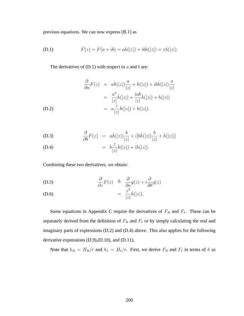
previous equations. We can now express (B.1) as

(D.1) F (z) = F (a+ ib) = ah(|z|) + ibh(|z|) = zh(|z|).

The derivatives of (D.1) with respect toa andb are:

∂

∂aF (z) = ah(|z|) a|z| + h(|z|) + ibh(|z|) a|z|

=a2

|z| h(|z|) +iab

|z| h(|z|) + h(|z|)

= az

|z| h(|z|) + h(|z|).(D.2)

∂

∂bF (z) = ah(|z|) b|z| + i[bh(|z|) b|z| + h(|z|)](D.3)

= bz

|z| h(|z|) + ih(|z|).(D.4)

Combining these two derivatives, we obtain:

∂

∂zF (z) ,

∂

∂ag(z) + i

∂

∂bg(z)(D.5)

=z2

|z| h(|z|).(D.6)

Some equations in Appendix C require the derivatives ofFR andFI . These can be

separately derived from the definition ofFR andFI or by simply calculating the real and

imaginary parts of expressions (D.2) and (D.4) above. This also applies for the following

derivative expressions (D.9),(D.10), and (D.11).

Note thathR = HR/r andhI = HI/r. First, we deriveFR andFI in terms ofh as

200

follows.

FR(z) = realF (z) = real(zh(|z|))

= reala(hR(|z|) + ihI(|z|)) + ib(hR(|z|) + ihI(|z|))

= ahR(|z|) − bhI(|z|).(D.7)

FI = imagF (z)

= imaga(hR(|z|) + ihI(|z|)) + ib(hR(|z|) + ihI(|z|))

= ahI(|z|) + bhR(|z|).(D.8)

The derivative of (D.7) and (D.8) with respect toa andb are:

∂

∂aFR =

∂

∂a(ahR(|z|) − bhI(|z|))

= hR(|z|) +a2

|z| hR(|z|) − ab

|z| hI(|z|).

∂

∂aFI =

∂

∂a(ahI(|z|) + bhR(|z|))

= hI(|z|) +a2

|z| hI(|z|) +ab

|z| hR(|z|).

∂

∂bFR =

∂

∂b(ahR(|z|) − bhI(|z|))

=ab

|z| hR(|z|) − hI(|z|) −b2

|z| hI(|z|).

∂

∂bFI =

∂

∂b(ahI(|z|) + bhR(|z|))

=ab

|z| hI(|z|) + hR(|z|) +b2

|z| hR(|z|).

201

The second derivatives ofF , which are used along with (C.6), (C.7), and (C.8) to find

c(y) in Appendix C are given by:

∂2

∂a2F (z) =

h(|z|)|z|

(z + 2a− a2 z

|z|2)

+h(|z|)|z|2

(az).(D.9)

∂2

∂b2F (z) =

h(|z|)|z|

(z + 2b− b2

z

|z|2)

+h(|z|)|z|2

(biz).(D.10)

∂

∂a

∂

∂bF (z) =

h(|z|)|z|

(ab+ ia− ab

z

|z|2)

+h(|z|)|z|2

(abz).(D.11)

The derivatives of the real and imaginary parts ofF are:

∂2

∂a2FR =

∂

∂a

(hR(|z|) +

a2

|z| hR(|z|) − ab

|z| hI(|z|))

=a

|z| hR(|z|) +2a

|z| hR(|z|) − a3

|z|2hR(|z|)

+a3

|z|2hR(|z|) − b

|z| hI(|z|) +a2b

|z|2hI(|z|)

−a2b

|z| hI(|z|).(D.12)

202

∂2

∂a2FI =

∂

∂a

(hI(|z|) +

a2

|z| hI(|z|) +ab

|z| hR(|z|))

=a

|z| hI(|z|) +2a

|z| hI(|z|) −a3

|z|2hI

+a3

|z|2hI +

b

|z| hR(|z|) − a2b

|z|2hR(|z|)

+a2b

|z|2hR(|z|).(D.13)

∂2

∂b2FR =

∂

∂b

(ab

|z| hR(|z|) − hI(|z|) −b2

|z| hI(|z|))

=a

|z| hR(|z|) − ab2

|z|2hR(|z|) − ab2

|z|2hR(|z|)

− b

|z| hI(|z|) −2b

|z| hI(|z|) +b3

|z|2hI(|z|)

− b3

|z|2hI(|z|).(D.14)

∂2

∂b2FI =

∂

∂b

(ab

|z| hI(|z|) + hR(|z|) +b2

|z| hR(|z|))

=a

|z| hI(|z|) −ab2

|z|2hI(|z|) +

ab2

|z|2hI(|z|)

+b

|z| hR(|z|) +2b

|z| hR(|z|) − b3

|z|2hR(|z|)

+b3

|z|2hR(|z|).(D.15)

∂

∂a

∂

∂bFR =

hR(|z|)|z| (b− a2b

|z| ) +hR(|z|)|z|2

(a2b) +

− hI(|z|)|z| (a− ab2

|z| ) −hI(|z|)|z|2

(ab2).(D.16)

203

∂

∂a

∂

∂bFI =

hI(|z|)|z| (b− a2b

|z| ) +hI(|z|)|z|2

(a2b)

+hR(|z|)|z| (a− ab2

|z| ) +hR(|z|)|z|2

(ab2).(D.17)

204

APPENDIX E

B1: Initial estimate for f and x

The estimator requires a good initial estimate forzk to ensure the estimator descends to

a good local minimum. We need an initial estimate for the magnitude and phase of theB+1

maps and of the object

The standard double angle method (5.2) is a natural choice for estimating the magni-

tude ofB+1 . The DAM effectively estimates the composite mapsxm (5.8); by forming

an appropriateα (defined below in (E.2)) and inverting it, we estimate the desired coil

mapszk. The DAM also requires that, for each composite map we estimate, we also take

a second measurement where the relative amplitude of each coil is double that of the first

measurement,i.e., letm = 2K and fixα such thatαm+k = 2αm wherem = 1, . . . , K. If

this condition is satisfied, we calculate the initial estimate z(0)k as follows.

First, we estimate the magnitude and phase of the composite maps. Using the corre-

sponding measurements (i.e., ym andym+k) in (5.2), we findx(0)m . Similarly, we use a

method of moments estimator for the phase ofB+1 :

(E.1) ∠xjm = ∠yjm − ∠H(|xjm|),

205

using our estimate of|xjm| from (5.2). We next form the matrix

(E.2) α =

α1

α2

...

αk

,

so that

α =

α

2α

.

Then, our initial estimate of theB+1 map is

z(0) = α−1x.(E.3)

Givenz(0), we estimate the objectf (0) using (5.7).

Alternatively, suppose that we only makeM = K + 1 measurements, the minimum

required to estimate both the object and each of the coil maps. We fix αK+1 = 2α1 as

before. Using these two measurements, we estimate thex1(0) andf (0) using (5.2), (E.1),

and (5.7). If the coil combinations are chosen wisely, this estimate should have few “holes”

and can be used as an initial estimate for the other coil combinationsi.e., x(0)m = x

(0)1 for

m = 2, . . . K + 1. Finally, we find theB+1 mapszm using (E.3) and the sameα matrix

(E.2) as before. We note, this estimate is not as good for the other coils and will likely

require more iterations and a higher SNR than if allM = 2K scans were used.

206

APPENDIX F

B1: What if α is complex?

Up to this point, we have assumed thatα consists of solely real values. However,

α could be complexe.g., if we put a different phase on each coil along with changing the

magnitude. This does make the derivation of cost function gradients and the final algorithm

more complicated. Let us look at these derivations more closely.

Now, letαmk = αRmk + iαI

mk andzjk = ajk + ibjk. Then,

real

K∑

k=1

αmkzjk

=

K∑

k=1

αRmkajk − αI

mkbjk,

and

imag

K∑

k=1

αmkzjk

=

K∑

k=1

αRmkbjk + αI

mkajk.

Now, bothreal∑K

k=1 αmkzjk

andimag

∑Kk=1 αmkzjk

contain bothajk andbjk. This

causes difficulty in evaluating (C.4), (C.5), (C.6), (C.7), or (C.8) when the argument for

a is real∑K

k=1 αmkzjk

and the argument forb is imag

∑Kk=1 αmkzjk

. For example,

whenα is real, we can use the chain rule to solve for∂∂ajk

G(a, b) and finally get the same

result as (D.2) with an extra factor ofαmk. Whenα is complex, however, (D.2) is no longer

suitable, because the new arguments “a” and “b” contain bothajk andbjk, so when we take

a derivative with respect toajk, we have to consider both “a” and “b”.

207

Therefore, we will require a new set of derivatives. Because∂∂aGR and ∂

∂aGI are re-

quired for all the second derivatives of the cost function (and we can solve all the first

derivatives of the cost function using only these derivatives), we solve for these, rather than

∂∂aG.

For shorthand, we let

real· , real

K∑

k=1

αmkzjk

,

and

imag· , imag

K∑

k=1

αmkzjk

,

and we recall that

|z| =

√√√√(K∑

k=1

ajk)2 + (K∑

k=1

bjk)2.

∂

∂ajk

FR =∂

∂ajk

(real·hR(|z|) − imag·hI(|z|))

= αRmkhR(|z|) + αR

mk

real2·|z| hR(|z|)

+αImk

real· imag·|z| hR(|z|) − αI

mkhI(|z|)

−αRmk

real· imag·|z| hI(|z|)

−αImk

imag2·|z| hI(|z|).

This expression is equivalent to the previous expression ifαImk = 0. We can see thatαmk

no longer factors simply out of these expressions; a naive incorrect application of the chain

rule to the previous expressions would yield wrong results.Similar results apply for the

208

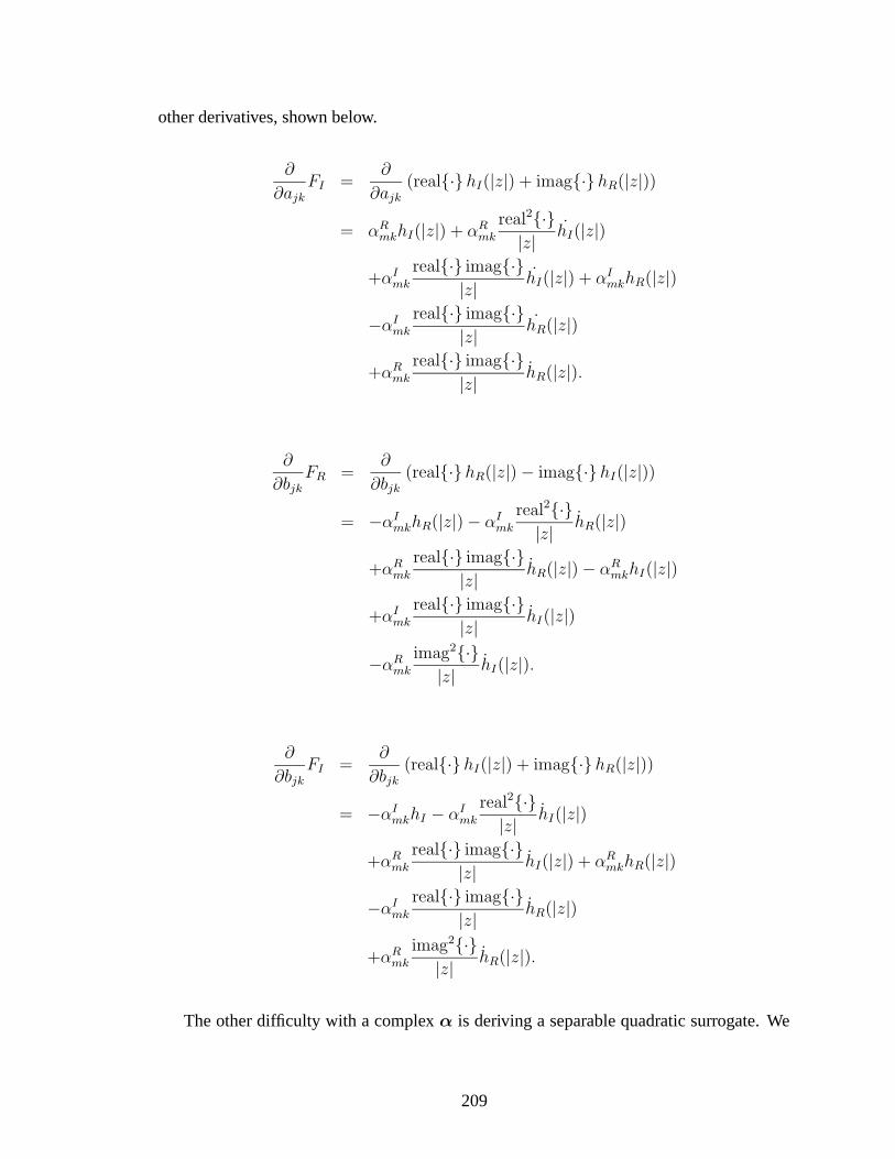
other derivatives, shown below.

∂

∂ajk

FI =∂

∂ajk

(real·hI(|z|) + imag·hR(|z|))

= αRmkhI(|z|) + αR

mk

real2·|z| hI(|z|)

+αImk

real· imag·|z| hI(|z|) + αI

mkhR(|z|)

−αImk

real· imag·|z| hR(|z|)

+αRmk

real· imag·|z| hR(|z|).

∂

∂bjkFR =

∂

∂bjk(real·hR(|z|) − imag·hI(|z|))

= −αImkhR(|z|) − αI

mk

real2·|z| hR(|z|)

+αRmk

real· imag·|z| hR(|z|) − αR

mkhI(|z|)

+αImk

real· imag·|z| hI(|z|)

−αRmk

imag2·|z| hI(|z|).

∂

∂bjkFI =

∂

∂bjk(real·hI(|z|) + imag·hR(|z|))

= −αImkhI − αI

mk

real2·|z| hI(|z|)

+αRmk

real· imag·|z| hI(|z|) + αR

mkhR(|z|)

−αImk

real· imag·|z| hR(|z|)

+αRmk

imag2·|z| hR(|z|).

The other difficulty with a complexα is deriving a separable quadratic surrogate. We

209

can no longer use the same definition ofπmk and finding a validπmk for this case seems

difficult at best. This is a matter for future work.

210

APPENDIX G

B1: Spatial Resolution Analysis

We must choose values for the regularization parameterβ to use the proposed regu-

larized method. With conventional regularization, this selection requires tedious trial-and-

error methods; preferably, values would be selected based on a quantitative measure, such

as the amount of smoothing to introduce. Therefore, we analyzed the spatial resolution

of the estimatedB+1 map z. To simplify the analysis, we focused on the single coil case

(K = 1) and assumed thatfj is known. Empirically, the spatial resolution of the multi-coil

case matched the spatial resolution of the single coil case when we usedM = 2K and a

uniform object and used the modified penalty described here.This analysis naturally led

to a modified penalty design, allowing for a standard selection of β based on desired blur

FWHM as well as providing more uniform spatial resolution independent of the particular

characteristics of theB+1 maps.

The local impulse response of the estimator is equal to the gradient of the estimator

multiplied by an impulse The gradient of the estimator has the following form:

∇z(y) = [∇[2,0] Ψ(z(y),y)]−1 −∇[1,1] Ψ(z(y),y)]

= [∇[2,0]L(z,y) + ∇2βR(z)]−1

[−∇[1,1]L(z,y)]|z=z(y),(G.1)

211

where∇[p,q] Ψ denotes thepth derivative ofΨ with respect toz and theqth derivative ofΨ

with respect toy.

The second derivative∇[2,0]L(z,y) introduces varying spatial resolution; this can par-

tially be accounted for through clever choice of the regularizer; therefore, we derive this

second derivative.

Becausez andy are both complex quantities, for this analysis we treat the real and

imaginary part of each as separate variables. We writezjks wherej denotes the voxel,k

denotes the coil, ands denotes the real or the imaginary part (thus,∂∂s

= ∂∂a

if s = R and

∂∂s

= ∂∂b

if s = I. Then, the Hessian ofL is:

[∇[2,0]L(z,y)]jks,j′k′s′ =

0 if j 6= j′

fjdjks;jk′s′(z) if j = j′,(G.2)

where

djks;jk′s′(z) =M∑

m=1

αmkαmk′

(∂

∂sFR([αzj]m)

∂

∂s′FR([αzj]m) +

∂

∂sFI([αzj]m)

∂

∂s′FI([αzj]m)

).(G.3)

For purposes of analysis, we used the mean measurement vector for y, i.e.

y = y = f F (x),

and then (G.3) has the same form as (C.6), (C.7), and (C.8) using appropriate values fors

and accounting for theαmk factors due to the chain rule for differentiation. Similarly, we

212

derived

[∇[1,1]L(x,y)]jks,j′m′s′ ,∂

∂zjks

∂

∂zj′k′s′L(z,y)

=

0 if j 6= j′

fjgj,k,s;j′,m′,s′ if j = j′,(G.4)

where

gj,k,s;j′,m′,s′ = αmk∂

∂sFs′([αz]m)

∂

∂sFs′(xjm′),(G.5)

again using the mean measurement vector. However, we note that as the regularization term

goes to zero, in the limit, then (G.4) times the gradient of the mean measurement vector

goes to (G.2) and understanding (G.4) becomes less necessary.

Although the Hessian is not “diagonal”, the diagonal elements are larger than the off-

diagonal elements. Therefore, we ignore the off-diagonal elements for the remainder of the

analysis.

The resulting spatial resolution for the estimatedB+1 maps shown in (G.2) is inherently

non-uniform. Areas with a low magnitudefj will be smoothed more because these areas

are more influenced by noise; this greater smoothing is desirable. Conversely, areas with

a large magnitude, which have a greater degree of data fidelity, are smoothed less. We

do not want the median magnitude offj to effect the amount of smoothing; therefore, we

normalize the data by the median value off in areas with large signal value (in this paper,

greater than 10% of the object maximum using the first-pass estimate of the object) giving

the object a median value of 1.

However, the effect ofdjks;jk′s′ seems less desirable. Therefore, we modified our

penalty using quadratic penalty design to create more uniform spatial resolution. This

approach is based on certainty-based Fisher information approximation [29, 34]. This ap-

proach requires an estimate ofz, which is unknown. Therefore, our first step is to run

213

the proposed algorithm through a few iterations (say,n = 5, wheren is the number of

iterations) to obtain a first-pass initial estimate ofz. We use a smallβ for the initial first

pass through the algorithm (e.g., we useβ = 2−10 in this paper), to allow a small level of

regularization. We then use this initialization to define a “certainty” factor as follows:

(G.6) κjks =√djks;jks(zn),

wherez(n) is our initial estimate. We note that becauseκjks is based on a noisy estimate

of z, areas wherefj is very small are particular noisy and create unreliable estimates forκ.

Therefore, we set these certainty factors in areas with small magnitude (in this paper, less

than 10% of the object maximum using the first-pass estimate of the object) to the average

value ofκ over the rest of the map. Then, we use the following modified penalty function:

(G.7) R(zk) =N∑

j=1

∑

l∈Nj

κjksκlks(zjks − zlks)2,

whereNj is a neighborhood of thejth pixel using second order differences. This creates

approximately uniform average spatial resolution iffj = 1. Thus, we eliminate most of the

effect ofdjks;jk′s′ from the spatial resolution, while still smoothing more in areas wherefj

is small.

Finally, we can now chooseβ based on the amount of acceptable blur. Assuming that

the modified penalty function (G.7) has madedjks;jk′s′ ≈ 1, we used the inverse 2D FFT to

compute the PSFz and tabulated its FWHM as a function ofβ/ |fj|. This graph is shown

in Fig 1 of [44]. Given the desired spatial resolution, we canpick the correspondingβ for

use in the algorithm. The resulting spatial resolution willbe inherently non-uniform, with

greater smoothing in low signal magnitude areas, effectively “interpolating” across signal

voids.

214

APPENDIX H

B1/T1: Derivatives of Signal Models: SSI and AFI

We consider both signals to be real to simplify analysis. We consider theB+1 map

and theT1 to be the two unknown variables and use the matrix CRB. For bothmodels,

we assume that the same echo time is used for both sequences, and, for the AFI, for both

repetition times. We also slightly modify the definition ofE1 andE2 to accommodate the

AFI pulse sequence

E1 = exp

(−TR1

T1

),

and

E2 = exp

(−TR2

T1

).

Then we can express the expectations as:

−E[∇2

T1ln p(F SSI

i ; b, T1

)]=

1

σ2

(1 − cos(φi)

1 − E1 cos(φi)

)2

·(

sin(φi)E1TR1

T 21 (1 − E1 cos(φi))

)2

.(H.1)

215

−E[∇T1∇b ln p

(F SSI

i ; b, T1

)]=

−1

σ2

αi(1 − E1)E1(cos(φi)−E1)

T 21 (1 − E1 cos(φi))4

·(1 − cos(φi)) sin(φi)TR.(H.2)

−E[∇2

b ln p(F SSI

i ; b, T1

)]=

1

σ2

(αi(1 − E1)

(1 − E1 cos(φi))2

)2

(cos(φi)−E1)2 .(H.3)

The relevant expressions for the CRB of the AFI are:

−E[∇2

b ln p(FAFI

2i−1 ; b, T1

)]=

1

σ2

(α

(1 − E1E2 cos2(φi))2

)2

(cos(φi) +E1E2 cos3(φi)−E2 cos(φi)

−E1E22 cos3(φi) +2E2 cos2(φi)−2E1E2 cos2(φi)

−E2 − E1E22 cos2(φi) +E1E2

+E21E

22 cos2(φi)−2E1E2 cos(φi) +2E1E

22 cos(φi)

)2

,(H.4)

and the expression forFAFI2i just replacesE1 with E2 and vice versa.

216

−E[∇b∇T1 ln p

(FAFI

1 ; b, T1

)]=

1

σ2

E2

T 21

α sin(φi)

(1 − E1E2 cos2(φi))4

(cos(φi) +E1E2 cos3(φi)−E2 cos(φi)

−E1E22 cos3(φi) +2E2 cos2(φi)−2E1E2 cos2(φi)

−E2 − E1E22 cos2(φi) +E1E2

+E21E

22 cos2(φi)−2E1E2 cos(φi) +2E1E

22 cos(φi)

)

(E1 cos(φi)(TR1 + TR2)(cos(φi) − 1)

+E1E2TR1 cos2(φi)(cos(φi) − 1)

−TR2 + TR2 cos(θ)

).(H.5)

−E[∇2

T1ln p(FAFI

2i−1 ; b, T1

)]=

1

σ2

(sin(φi)

(1 − E1E2 cos2(φi))2

)2(E2

T 21

)2

(E1 cos(φi)(TR1 + TR2)(cos(φi) − 1)

+E1E2TR1 cos2(φi)(cos(φi) − 1)

−TR2 + TR2 cos(φi)

)2

.(H.6)

217

APPENDIX I

B+1 ,T1: Derivation of cost function gradients

This section first considers a simplified version of theB+1 andT1 map cost function

and its gradient. Any gradient-based algorithm uses the first derivative of the cost function.

Next, we apply the results to our cost function (6.19). The equations in this section rely

heavily on derivatives of the functionF which are derived (in terms of derivatives ofH)

in Appendix J (and are very similar to those in Appendix C withthe addition of a third

parameter forT1).

First, consider a simple (one voxel, one measurement) version of (6.20). We can rewrite

(6.20) as follows:

L(z, t, f) = l

(y, t, f, real

K∑

k=1

αkzk

, imag

K∑

k=1

αkzk

)

l(y, t, f, a, b) ,1

2|y − fG(a, b, t)|2

G(a, b, t) , F (a+ ib, t) = GR(a, b, t) + iGI(a, b, t),(I.1)

wherez = (z1, . . . , zK).

We simplify l(·) by ignoring terms independent of the unknown variablesa or b (and

218

recalling thatf is constrained to be real):

l(y, t, f, a, b) , − realy realfG(a, b, t)

− imagy imagfG(a, b, t)

+1

2|f |2 |G(a, b, t)|2 .(I.2)

l(y, t, f, a, b) ≡ −yRfGR(a, b, t) − yIfGI(a, b, t)

+1

2f 2 |G(a, b, t)|2 .(I.3)

The derivative ofl with respect to the unknown variablea is:

∂

∂al = −yRf

∂

∂aGR(a, b, t) − yIf

∂

∂aGI(a, b, t)

+f 2GR(a, b, t)∂

∂aGR(a, b, t)

+f 2GI(a, b, t)∂

∂aGI(a, b, t)

= −f(yR − fGR(a, b, t))∂

∂aGR(a, b, t)

−f(yI − fGI(a, b, t))∂

∂aGI(a, b, t)

= −f(yR − fGR(a, b, t))∂

∂aGR(a, b, t)

+if(yI − fGI(a, b, t))i∂

∂aGI(a, b, t)

= −f real

(y − fG(a, b, t))∗

∂

∂aG(a, b, t)

.(I.4)

219

Similarly, the derivative with respect tob is:

∂

∂bl = −yRf

∂

∂bGR(a, b, t) − yIf

∂

∂bGI(a, b, t)

+ |f |2GR(a, b, t)∂

∂bGR(a, b, t)

+ |f |2GI(a, b, t)∂

∂bGI(a, b, t)

= −f real

(y − fG(a, b, t))∗

∂

∂bG(a, b, t)

.(I.5)

Similarly, the derivative with respect tot is:

∂

∂tl = −yRf

∂

∂tGR(a, b, t) − yIf

∂

∂tGI(a, b, t)

+ |f |2GR(a, b, t)∂

∂tGR(a, b, t)

+ |f |2GI(a, b, t)∂

∂tGI(a, b, t)

= −f real

(y − fG(a, b, t))∗

∂

∂tG(a, b, t)

.(I.6)

When regularizing the object, the derivative with respect tof is needed. The derivative is:

∂

∂fl = −yRGR(a, b, t) − yIGI(a, b, t) + |f | |G(a, b, t)|2 .(I.7)

.

We also include the second derivatives for use in a Hessian calculation (for example,

for a preconditioner for gradient descent algorithms, although not currently implemented

in the algorithm). The second derivative ofl with respect to the unknown variablea is:

∂2

∂a2l = −f(yR − fGR(a, b, t))

∂2

∂a2GR(a, b, t)

−f(yI − fGI(a, b, t))∂2

∂a2GI(a, b, t)

+ |f |2((

∂

∂aGR(a, b, t)

)2

+

(∂

∂aGI(a, b, t)

)2).(I.8)

220

Similarly, the second derivative ofl with respect to the unknown variableb is:

∂2

∂b2l = −f(yR − fGR(a, b, t))

∂2

∂b2GR(a, b, t)

−f(yI − fGI(a, b, t))∂2

∂b2GI(a, b, t)

+ |f |2((

∂

∂bGR(a, b, t)

)2

+

(∂

∂bGI(a, b, t)

)2).(I.9)

The second derivative ofl with respect to the unknown variablet is:

∂2

∂t2l = −f(yR − fGR(a, b, t))

∂2

∂t2GR(a, b, t)

−f(yI − fGI(a, b, t))∂2

∂t2GI(a, b, t)

+ |f |2((

∂

∂tGR(a, b, t)

)2

+

(∂

∂tGI(a, b, t)

)2).(I.10)

The second derivative ofl with respect to the unknown variablef is:

∂2

∂f 2l = |G(a, b, t)|2 .(I.11)

221

APPENDIX J

B+1 , T1: Derivatives of F

This section derives the derivatives ofF in terms ofH and its derivatives, which are

tabulated (when using a non-ideal slice profile or incorporating B0 field inhomogeneity)

or explicitly derived (assuming an ideal sinc profile as the experiments in this thesis) as

explained in Section 6.5.1.

To simplify the derivations, we use an equivalent definitionfor F . We definez = a+ ib

and rewrite (6.26) as follows:

F (z, t) = eı∠z H(√a2 + b2, t)

=

(a√

a2 + b2+

ib√a2 + b2

)H(

√a2 + b2, t).

The final line follows from using Euler’s formula foreı∠z and expressingcos andsin using

the Pythagorean Theorem.

Then,

FR(a, b, t) =a√

a2 + b2HR(

√a2 + b2, t) − b√

a2 + b2HI(

√a2 + b2, t)

FI(a, b, t) =b√

a2 + b2HR(

√a2 + b2, t) +

a√a2 + b2

HI(√a2 + b2, t).

222

Using these equations, we can then find the derivatives

d

daFR(a, b, t) =

1

|z|HR(|z| , t) − a2

|z|2HR(|z| , t) +

a2

|z|2∇[10]HR(|z| , t)

+ab

|z|2HI(|z| , t) −

ab

|z|2∇[10]HI(|z| , t)

d

dbFR(a, b, t) =

−1

|z|HI(|z| , t) −ab

|z|2HR(|z| , t) +

ab

|z|2∇[10]HR(|z| , t)

+b2

|z|2HI(|z| , t) −

b2

|z|2∇[10]HI(|z| , t)

d

daFI(a, b, t) =

1

|z|HI(|z| , t) −a2

|z|2HI(|z| , t) +

a2

|z|2∇[10]HI(|z| , t)

− ab

|z|2HR(|z| , t) +

ab

|z|2∇[10]HR(|z| , t)

d

dbFI(a, b, t) =

1

|z|HR(|z| , t) − ab

|z|2HI(|z| , t) +

ab

|z|2∇[10]HI(|z| , t)

− b2

|z|2HR(|z| , t) +

b2

|z|2∇[10]HR(|z| , t)

d

dtFR(a, b, t) = cos(∠z)∇[01]HR(|z| , t) − sin(∠z)∇[01]HI(|z| , t)

= ℜ(exp(i∠z)∇[01]H(|z| , t)

)

d

dtFI(a, b, t) = cos(∠z)∇[01]HI(|z| , t) + sin(∠z)∇[01]HR(|z| , t)

= ℑ(exp(i∠z)∇[01]H(|z| , t)

).

223

APPENDIX K

B+1 , T1: Initial estimate for B+

1 , T1, and f

The algorithm requires a good initial estimate forB+1 andT1 to ensure the iterates

descends to a good local minimum. We need an initial estimatefor the magnitude and

phase of theB+1 maps, theT1 map, and the object.

Simple approach - AssumeTR = ∞

We note that the standard approach forT1 estimation (based on (6.14) assumes that the

flip angle (and thus, theB+1 map) is known. Then,T1 is estimated from the data using a

transformation of the points and using a least-squares fit. Therefore, one approach to joint

initial estimates is finding a goodB+1 estimate and then use the standardT1 estimate and

use (6.24) to estimate the object. One obvious choice is assuming thatTR = ∞ and using

the standard double angle method using for estimating the magnitude ofB+1 . We use a

method of moments estimator for the phase ofB+1 :

∠xjm = ∠yjm − ∠H(|xjm|,Tj

),(K.1)

using our estimate of|xjm|, wherexm are the composite maps (6.25). (Note thatH is

defined in (6.26).) Empirically, we found that while the phaseB+1 maps are of sufficiently

224

good quality, the magnitudeB+1 maps, assuming an infinite repetition time, can be greatly

improved.

An improvement over this method is using the regularizedB+1 estimates from Chap-

ter V with a small number of iterations. Generally, the more initial estimates introduced

later in this appendix are based on our improved model and therefore perform better. How-

ever, with a low SNR, especially when only one coil is “on” at atime as in OAAT, the

regularizedB+1 estimate is more robust to noise and can work quite well. Thismethod

also has the advantage of only requiringM = 2 ∗ K, though all estimates show theT1

effects. One option is generating both the more complicatedinitial estimates as well as the

simpleB+1 estimate described above and choosing the one with less error compared to the

measured data.

Triple angle method for multiple tip angles and constant TR

For our jointB+1 /T1 estimation, we used the following initialization when the TR is

constant and there is a wide range of tip angles (see examplesin Section 6.6.1). First, we

write the simplified SSI signal model as:

Si = A sinαib1 −X

1 − cosαibX,(K.2)

where

X = exp

(−TRT1

),

and

T1 =−TRlogX

.

Similar to the double angle method (5.1) and (5.2), we require three signals such that

α2 = 2α1

α3 = 3α1.

225

Therefore, this method requires at leastM = 3 ∗ K. If we let c , cos(α1b), using the

double and triple angle trigonometric identities, then

cos(α2b) = 2c2 − 1

cos(α3b) = 4c3 − 3c

sin(α1b) =√

1 − c2

sin(α2b) = 2c√

1 − c2

sin(α3b) = 3√

1 − c2 − 4(√

1 − c2)3

.

We then define the following ratios

z2 =|S2||S1|

=sin(α2b)

sin(α1b)· 1 − cos(α1b)X

1 − cos(α2b)X

=2c(1 − cX)

1 − (2c2 − 1)X(K.3)

and

z3 =|S3||S1|

=sin(α3b)

sin(α1b)· 1 − cos(α1b)X

1 − cos(α3b)X

= (3 − 4(1 − c2)) · 1 − cX

1 − (4c3 − 3c)X.(K.4)

Then, we solvez2 for X:

X =z2 − 2c

z2(2c2 − 1) − 2c2.(K.5)

226

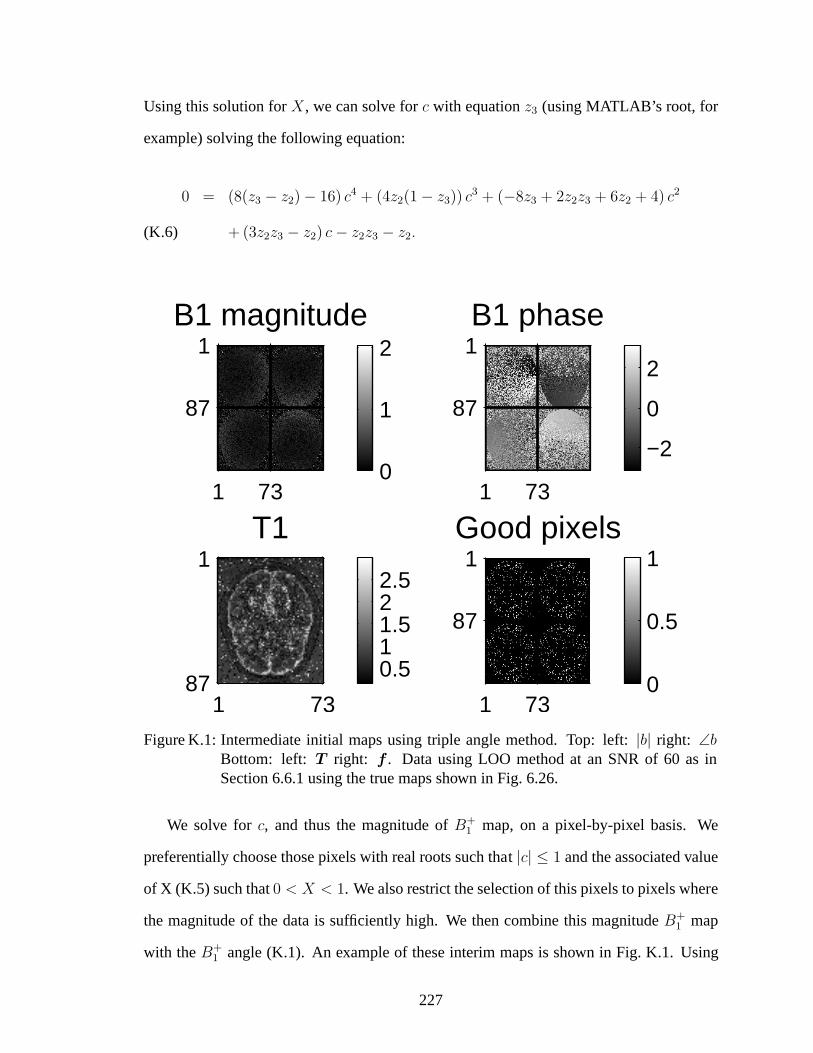
Using this solution forX, we can solve forc with equationz3 (using MATLAB’s root, for

example) solving the following equation:

0 = (8(z3 − z2) − 16) c4 + (4z2(1 − z3)) c3 + (−8z3 + 2z2z3 + 6z2 + 4) c2

+ (3z2z3 − z2) c− z2z3 − z2.(K.6)

B1 magnitude

1 73

1

87

0

1

2B1 phase

1 73

1

87

−2

0

2

T1

1 73

1

870.511.522.5

Good pixels

1 73

1

87

0

0.5

1

Figure K.1: Intermediate initial maps using triple angle method. Top: left: |b| right: ∠bBottom: left: T right: f . Data using LOO method at an SNR of 60 as inSection 6.6.1 using the true maps shown in Fig. 6.26.

We solve forc, and thus the magnitude ofB+1 map, on a pixel-by-pixel basis. We

preferentially choose those pixels with real roots such that |c| ≤ 1 and the associated value

of X (K.5) such that0 < X < 1. We also restrict the selection of this pixels to pixels where

the magnitude of the data is sufficiently high. We then combine this magnitudeB+1 map

with theB+1 angle (K.1). An example of these interim maps is shown in Fig.K.1. Using

227

the complexB+1 map values at the preferred pixels, we fit a two-dimensional polynomial

function over the entire object (in this thesis, we use a fourth degree polynomial) for both

the real and imaginary values ofB+1 . (We note that fitting instead to the magnitude and

phase ofB+1 would require meeting the constraint that|b| ≥ 0.)

Finally, we use this new fittedB+1 map and (K.5) to get our initial estimate ofT1. This

does seem susceptible to noise when the SNR is low (e.g., around 30) but produces very

good estimates with low noise and is used for the simulations. The final initial maps for

this example are shown in Section 6.6.1 in Fig. 6.32, Fig. 6.33, Fig. 6.34, and Fig. 6.35.

Method when TR is varied

When we use the same flip angle for each measurement and insteadvary the repetition

time TR , neither of the above initializations apply. Here is another possible initialization

method that we used with the phantom data described in Section 6.6.2. This method works

when we have a good estimate of theT1 map. In the phantom data, we knew thatT1 was

roughly constant over the object and the approximate value (T = 1 ms for the phantom

used in this thesis). With this information, we fit, voxel by voxel,B+1 using the SSI model

(6.27) assuming thatT1 is known and fixed by minimizing the norm of the difference (for

example, using MATLAB’s fminsearch). For the first set of phantom data, this initialB+1 is

shown in Fig. K.2. We estimate the phase ofB+1 using (K.1). By normalizing the data with

respect to a reference image, we also calculatedf over the object and setf to a constant

value equal to its estimated mean.

When a combination of coils is used, we estimate theB+1 maps for the composite maps

(5.8). One option is using these maps to estimate the composite maps and then finally

solve for the individual maps at the end. This may not be desirable when there are coil

cancellations. Another option is immediately estimating the individual coils

As in the triple angle method, we improve the initialB+1 map estimate by fitting a

fourth order polynomial to weighted|b| values inside the object (the weights inversely

228

Jons B1 init (cost fxn minimizied)

1 64

1

64

0

0.2

0.4

0.6

0.8

1

1.2

1.4

1.6

Figure K.2: Intermediate initialB+1 map when TR is varied. Initial OAAT phantom exper-

imentB+1 estimate assuming knownT1.

proportional to the error of the data as measured between themeasured magnitude data and

the current estimated magnitude data). These initial estimates are shown in Fig. 6.45 for

the first phantom experiment.

From the improved complexB+1 map estimate, we calculated an improvedT1 map

estimate using the standardT1 estimate and an improvedf map estimate using (6.24).

229

APPENDIX L

B+1 , T1: Spatial Resolution Analysis

We must choose values for the regularization parametersβ to use the proposed regu-

larized method. With conventional regularization, this selection requires tedious trial-and-

error methods; preferably, values would be selected based on a quantitative measure, such

as the amount of smoothing to introduce.

Therefore, we analyzed the spatial resolution of the estimatedB+1 mapz andT1 map

T and thef f .

To simplify the analysis, we focused on the single coil case (K = 1). ForB+1 map

estimation, we assumed thatfj andT are known and fixed; forT1 map estimation, we

assumed thatfj andb are known and fixed. Empirically, the spatial resolution of the multi-

coil case matched the spatial resolution of the single coil case when we usedM = 4K and

a uniform object and used the modified penalty described here. This analysis naturally led

to a modified penalty design, allowing for a standard selection of β based on desired blur

FWHM as well as providing more uniform spatial resolution independent of the particular

characteristics of theB+1 maps. Without this analysis, in conventional regularization each

map would have (possibly drastically) different spatial resolution when using the sameβ.

The goal of this analysis is that, when using the sameβ, an impulse added to the true map

will result in a certain full-width half-maximum in the finalestimated map.

230

The local impulse response of the estimator is equal to the gradient of the estimator

multiplied by an impulse. The gradient of the estimator has the following general form

(wherey is the data andz is the variable):

∇z(y) = [∇[2,0] Ψ(z(y),y)]−1 −∇[1,1] Ψ(z(y),y)]

= [∇[2,0]L(z,y) + ∇2βR(z)]−1

[−∇[1,1]L(z,y)]|z=z(y),(L.1)

where∇[p,q] Ψ denotes thepth derivative ofΨ with respect toz and theqth derivative ofΨ

with respect toy.

The second derivative∇[2,0]L(z,y) introduces varying spatial resolution; this can par-

tially be accounted for through clever choice of the regularizer; therefore, we derive this

second derivative.

First, we consider the spatial resolution of theB+1 mapz. Becausez andy are both

complex quantities, for this analysis we treat the real and imaginary part of each as separate

variables. We writezjks wherej denotes the voxel,k denotes the coil, ands denotes the

real or the imaginary part (thus,∂∂s

= ∂∂a

if s = R and ∂∂s

= ∂∂b

if s = I). Then, the Hessian

of L is:

[∇[2,0]L(z,y)]jks,j′k′s′ =

0 if j 6= j′

fjdjks;jk′s′(z) if j = j′,(L.2)

where

djks;jk′s′(z) =M∑

m=1

αmkαmk′

(∂

∂sFR([αzj]m, tj)

∂

∂s′FR([αzj]m, tj) +

∂

∂sFI([αzj]m, tj)

∂

∂s′FI([αzj]m, tj)

).(L.3)

231

For purposes of analysis, we used the mean measurement vector for y, i.e.

y = y = f F (x, t),

and then (L.3) has the same form as (I.8) and (I.9). using appropriate values fors and ac-

counting for theαmk factors due to the chain rule for differentiation. Similarly, we derived

[∇[1,1]L(x,y)]jks,j′m′s′ ,∂

∂zjks

∂

∂zj′k′s′L(z,y)

=

0 if j 6= j′

fjgj,k,s;j′,m′,s′ if j = j′,(L.4)

where

gj,k,s;j′,m′,s′ = αmk∂

∂sFs′([αzj]m, tj)

∂

∂sFs′([αzj]m′ , tj),(L.5)

again using the mean measurement vector. However, we note that as the regularization

term goes to zero, in the limit, then (L.4) times the gradientof the mean measurement

vector goes to (L.2) and understanding (L.4) becomes less necessary.

We repeated this analysis for an unknownT1 mapT with a knownB+1 mapz and object

f . Now, the Hessian ofL is:

[∇[2,0]L(T ,y)]j,j′ =

0 if j 6= j′

f 2j dj;j(z) if j = j′

,(L.6)

where

dj;j(z) =M∑

m=1

(∂

∂tFR ([αzj]m, tj)

)2

+

(∂

∂tFI ([αzj]m, tj)

)2

.(L.7)

232

We note that the variable transformation ofT slightly modifies this equation as explained

in Section M.

We repeated this analysis for an unknown object map (assuming that we are regularizing

the object)f with a knownT1 mapT andB+1 mapz. Now, the Hessian ofL is:

[∇[2,0]L(f ,y)]j,j′

0 if j 6= j′

rj,j(z) if j = j′,(L.8)

where

rj;j(z) =M∑

m=1

(FR ([αzj]m, tj))2 +

(FI ([αzj]m, tj))2 .(L.9)

Although these Hessians are not “diagonal”, the diagonal elements are larger than the

off-diagonal elements. Therefore, we ignore the off-diagonal elements for the remainder

of the analysis.

The resulting spatial resolution for the estimated maps shown in (L.2), (L.6), and (L.8)

is inherently non-uniform. Areas with a low magnitudefj will be smoothed more because

these areas are more influenced by noise; this greater smoothing is desirable. Conversely,

areas with a large magnitude, which have a greater degree of data fidelity, are smoothed

less. We do not want the median magnitude offj to effect the amount of smoothing;

therefore, we normalize the data by the median value off in areas with large signal value

(in this paper, greater than 10% of the object maximum using the first-pass estimate of the

object) giving the object a median value of 1.

However, the effect ofdjks;jk′s′ anddj,j andrj,j seems less desirable. Therefore, we

modified our penalties using quadratic penalty design to create more uniform spatial resolu-

tion. This approach is based on certainty-based Fisher information approximation [29,34].

This approach requires an estimate ofb or T or f , which is unknown. One option is is to

233

run the proposed algorithm through a few iterations (say,n = 5, wheren is the number of

iterations) to obtain a first-pass initial estimate ofz andT . and then use a smallβ for the

initial first pass through the algorithm (e.g., β = 2−10), to allow a small level of regular-

ization. A second option is to use the initial values ofz or T used for the algorithm; we

found the estimates described in Appendix K were sufficiently accurate to use to calculate

an improved regularization scheme.

We then use these estimates to define a “certainty” factor as follows:

(L.10) κzjks =

√djks;jks(zn),

and

(L.11) κTj =

√dj;j(T n),

and

(L.12) κfr =

√rj;j(fn

j ),

wherez(n) andT (n) are our initial estimates. We note that becauseκzjks andκT

j andκfr are

based on a noisy estimate ofz or T or f , areas wherefj is very small are particular noisy

and create unreliable estimates forκz andκT andκfj . Therefore, we set these certainty

factors in areas with small magnitude (in this paper, less than 10% of the object maximum

using the first-pass estimate of the object) to the average value ofκ over the rest of the map.

Then, we use the following modified penalty function:

(L.13) R(zk) =N∑

j=1

∑

l∈Nj

κzjksκ

zlks(zjks − zlks)

2,

234

and

(L.14) R(T ) =N∑

j=1

∑

l∈Nj

κTj κ

Tl (Tj − Tl)

2,

and

(L.15) R(fj) =N∑

j=1

∑

linNj

κTr κ

fl (fj − fl)

2,

whereNj is a neighborhood of thejth pixel using second order differences. This creates

approximately uniform average spatial resolution iffj = 1 and assuming quadratic regular-

ization. When tested under these assumptions, spatial resolution is quite uniform forB+1 .

Using the improved penalty (L.14) forT1 (with quadratic regularization and a testT1 with

blocks of varyingT1 values) still results in some spatial resolution variationbut is more

uniform and predictable than the original penalty. However, when all other variables are

known and kept constant, the improved penalty gives much more uniform spatial resolu-

tion. Thus, using the improved penalties (L.13) and (L.14) we eliminate most of the effect

of djks;jk′s′ anddj,j from the spatial resolution, while still smoothing more in areas where

fj is small.

Finally, we can now chooseβ based on the amount of acceptable blur. Assuming that

the modified penalty function (L.13) has madedjks;jk′s′ ≈ 1 and (L.14) has madedj;j ≈ 1

and (L.15) has maderj;j ≈ 1, we can chose a FWHM as a function ofβ/ |fj| based on the

graph shown in Fig. 4.1. Given the desired spatial resolution, we can pick the corresponding

β for use in the algorithm. The resulting spatial resolution will be inherently non-uniform,

with greater smoothing in low signal magnitude areas, effectively “interpolating” across

signal voids.

235

APPENDIX M

B+1 , T1: Constrained estimation for T1

T1 is physically constrained to be positive. Therefore, we wish to constrain

0 ≤ T < TMAX ,

where we letTMAX be equal to the maximum value ofT1 we could physically expect in

the field of view. In this paper, we setTMAX = 3 s. To enforce these constraints, we let

T = Γ(ς) where we choseΓ to be the sigmoid function

Γ(ς) =TMAX

1 + exp(−ς) .(M.1)

We then estimate the new variableς. The cost function (6.19) becomes

(z, T , f) = arg minz,T :0<Tj<TMAX ,f

Ψ(z,T ,f),

(z, ς , f) = arg minz,ς,f

Ψ(z, ς,f),

Ψ(z, ς,f) = L(z,Γ(ς),f) + βzR(z) + βςR(ς).(M.2)

Finally, we letTj = Γ (ς).

236

We note that the cost function gradients as derived in Section I change only via the

chain rule with the additional multiplication of the following factor:

∂

∂ςΓ(ς) =

TMAX exp−ς

(1 + exp−ς)2 .(M.3)

Then,∂

∂ςjΨ(z,T ,f) =

(∂

∂Tj

L(z,T ,f)

)|T=Γ(ς) · ˙Γ(ςj) +

∂

∂ςjβςR(ς).

The spatial resolution also changes slightly. As we are estimating and regularizingς

(L.11) will also require the additional multiplication factor (M.3) shown above.

In this paper, we first estimateT1 as explained in Section K and then convert this via

the inverse logistic function

ς = − ln

(TMAX

T− 1

)

and then solve forς as above. Finally, we convert this back into aT1 map via (M.1).

237

BIBLIOGRAPHY

238

BIBLIOGRAPHY

[1] H. Erdogan and J. A. Fessler. Ordered subsets algorithms for transmission tomogra-phy. Phys. Med. Biol., 44(11):2835–51, November 1999.

[2] S. Akoka, F. Franconi, F. Seguin, and A. Le Pape. Radiofrequency map of an NMRcoil by imaging.Mag. Res. Im., 11(3):437–41, 1993.

[3] P. Aksit, J. A. Derbyshire, and J. L. Prince. Three-pointmethod for fast and robustfield mapping for EPI geometric distortion correction. InProc. IEEE Intl. Symp.Biomed. Imag., pages 141–4, 2007.

[4] B. Aubert-Broche, A. C. Evans, and D. L. Collins. A new improved version of therealistic digital brain phantom.neuroimage, 32(1):138–45, August 2006.

[5] B. Aubert-Broche, M. Griffin, G. B. Pike, A. C. Evans, and D.L. Collins. Twentynew digital brain phantoms for creation of validation imagedata bases.IEEE Trans.Med. Imag., 25(11):1410–6, November 2006.

[6] M. A. Bernstein, M. Grgic, T. J. Brosnan, and N. J. Pelc. Reconstructions of phasecontrast, phased array multicoil data.Mag. Res. Med., 32(3):330–334, September1994.

[7] K. T. Block, M. Uecker, and J. Frahm. Undersampled radialMRI with multiplecoils. Iterative image reconstruction using a total variation constraint. Mag. Res.Med., 57(6):1086–98, June 2007.

[8] D. Bohning and B. G. Lindsay. Monotonicity of quadratic approximation algo-rithms. Ann. Inst. Stat. Math., 40(4):641–63, December 1988.

[9] L. Bokacheva, A. J. Huang, Q. Chen, N. Oesingmann, P. Storey, H. Rusinek, andV. S. Lee. Single breath-holdT1 measurement using low flip angle TrueFISP.Mag.Res. Med., 55(5):1186–90, May 2006.

[10] D. Brunner and K. Pruessmann. A matrix approach for mapping array transmit fieldsin under a minute. InProc. Intl. Soc. Mag. Res. Med., page 354, 2008.

[11] D. O. Brunner and K. P. Pruessmann. B1+ interferometry for the calibration of RFtransmitter arrays.Mag. Res. Med., 61(6):1480–8, June 2009.

239

[12] M. F. Callaghan, J. L. Ulloa, D. J. Larkman, P. Irarrazaval, and J. V. Hajnal. Mea-suring coil sensitivities of transmit and receive arrays with demonstration of RFshimming. InProc. Intl. Soc. Mag. Res. Med., page 2627, 2006.

[13] M. A. Castro, J. Yao, Y. Pang, C. Lee, E. Baker, J. Butman, I.E. Evangelou, andD. Thomasson. Template-based B1 inhomogeneity correctionin 3T MRI brain stud-ies. IEEE Trans. Med. Imag., 29(11):1927–41, November 2010.

[14] L-C. Chang, C. G. Koay, P. J. Basser, and C. Pierpaoli. Linearleast-squares methodfor unbiased estimation of T1 from SPGR signals.Mag. Res. Med., 60(2):496–501,August 2008.

[15] N. Chen and A. M. Wyrwicz. Correction for EPI distortions using multi-echogradient-echo imaging.Mag. Res. Med., 41(6):1206–13, June 1999.

[16] H-L. M. Cheng and G. A. Wright. Rapid high-resolutionT1 mapping by variableflip angles: Accurate and precise measurements in the presence of radiofrequencyfield inhomogeneity.Mag. Res. Med., 55(3):566–74, March 2006.

[17] P. L. Choyke, A. J. Dwyer, and M. V. Knopp. Functional tumor imaging with dy-namic contrast-enhanced magnetic resonance imaging.J. Mag. Res. Im., 17(5):509–20, May 2003.

[18] D. L. Collins, A. P. Zijdenbos, V. Kollokian, J. G. Sled, N. J. Kabani, C. J. Holmes,and A. C. Evans. Design and construction of a realistic digital brain phantom.IEEETrans. Med. Imag., 17(3):463–8, June 1998.

[19] R. T. Constable, R. C. Smith, and J. C. Gore. Signal-to-noise and contrast in fastspin echo (FSE) and inversion recovery FSE imaging.J. Comp. Assisted Tomo.,16:41–7, 1992.

[20] C. H. Cunningham, J. M. Pauly, and K. S. Nayak. Saturated double-angle methodfor rapidB1+ mapping.Mag. Res. Med., 55(6):1326–33, June 2006.

[21] R. Cusack, M. Brett, and K. Osswald. An evaluation of the use of magnetic field-maps to undistort echo-planar images.NeuroImage, 18(1):127–42, January 2003.

[22] A. R. De Pierro. A modified expectation maximization algorithm for penalized like-lihood estimation in emission tomography.IEEE Trans. Med. Imag., 14(1):132–7,March 1995.

[23] R. Deichmann. Fast high-resolutionT1 mapping of the human brain.Mag. Res.Med., 54(1):20–7, July 2005.

[24] S. C. L. Deoni. High-resolution T1 mapping of the brain at3T with driven equilib-rium single pulse observation of T1 with high-speed incorporation of RF field inho-mogeneities (DESPOT1-HIFI).J. Mag. Res. Im., 26(4):1106–11, October 2007.

240

[25] S. C. L. Deoni, T. M. Peters, and B. K. Rutt. Determinationof optimal angles forvariable nutation proton magnetic spin-lattice,T1, and spin-spin,T2, relaxation timesmeasurement.Mag. Res. Med., 51(1):194–9, January 2004.

[26] S. C. L. Deoni, B. K. Rutt, and T. M. Peters. Rapid combinedT1 and T2 mappingusing gradient recalled acquisition in the steady state.Mag. Res. Med., 49(3):515–26, March 2003.

[27] J. A. Detre, J. S. Leigh, D. S. Williams, and A. P. Koretsky. Perfusion imaging.Mag. Res. Med., 23(1):37–45, January 1992.

[28] N. G. Dowell and P. S. Tofts. Fast, accurate, and precisemapping of the RF field invivo using the1800 signal null.Mag. Res. Med., 58(3):622–30, September 2007.

[29] J. A. Fessler. Mean and variance of implicitly defined biased estimators (such as pe-nalized maximum likelihood): Applications to tomography.IEEE Trans. Im. Proc.,5(3):493–506, March 1996.

[30] J. A. Fessler.Image reconstruction: Algorithms and analysis. ?, 2006. Book inpreparation.

[31] J. A. Fessler, N. H. Clinthorne, and W. L. Rogers. On complete data spaces for PETreconstruction algorithms.IEEE Trans. Nuc. Sci., 40(4):1055–61, August 1993.

[32] J. A. Fessler, S. Lee, V. T. Olafsson, H. R. Shi, and D. C. Noll. Toeplitz-based itera-tive image reconstruction for MRI with correction for magnetic field inhomogeneity.IEEE Trans. Sig. Proc., 53(9):3393–402, September 2005.

[33] J. A. Fessler and D. C. Noll. Iterative image reconstruction in MRI with separatemagnitude and phase regularization. InProc. IEEE Intl. Symp. Biomed. Imag., pages209–12, 2004.

[34] J. A. Fessler and W. L. Rogers. Uniform quadratic penalties cause nonuniform im-age resolution (and sometimes vice versa). InProc. IEEE Nuc. Sci. Symp. Med. Im.Conf., volume 4, pages 1915–9, 1994.

[35] J. A. Fessler and W. L. Rogers. Spatial resolution properties of penalized-likelihoodimage reconstruction methods: Space-invariant tomographs. IEEE Trans. Im. Proc.,5(9):1346–58, September 1996.

[36] J. A. Fessler and B. P. Sutton. Nonuniform fast Fourier transforms using min-maxinterpolation.IEEE Trans. Sig. Proc., 51(2):560–74, February 2003.

[37] J. A. Fessler, D. Yeo, and D. C. Noll. Regularized fieldmapestimation in MRI. InProc. IEEE Intl. Symp. Biomed. Imag., pages 706–9, 2006.

[38] L. Fleysher, R. Fleysher, S. Liu, W. Zaaraoui, and O. Gonen. Optimizing theprecision-per-unit-time of quantitative MR metrics: Examples forT1, T2, and DTI.Mag. Res. Med., 57(2):380–7, February 2007.

241

[39] R. Fleysher, L. Fleysher, M. Inglese, and D. Sodickson.TROMBONE: T1-relaxation-oblivious mapping of transmit radio-frequency field (B1) for MRI at highmagnetic fields.Mag. Res. Med., 2011.

[40] A. Funai and J. A. Fessler. Cramer Rao bound analysis of joint B1/T1 mappingmethods in MRI. InProc. IEEE Intl. Symp. Biomed. Imag., pages 712–5, 2010.

[41] A. Funai, J. A. Fessler, W. Grissom, and D. C. Noll. Regularized B1+ map estima-tion in MRI. In Proc. IEEE Intl. Symp. Biomed. Imag., pages 616–9, 2007.

[42] A. K. Funai, J. A. Fessler, W. Grissom, and D. C. Noll. Regularized B1+ mapestimation with slice selection effects. InProc. Intl. Soc. Mag. Res. Med., page3145, 2008.

[43] A. K. Funai, J. A. Fessler, and D. C. Noll. Estimating K transmit B1+ maps fromK+1 scans for parallel transmit MRI. InProc. Intl. Soc. Mag. Res. Med., page 2609,2009.

[44] A. K. Funai, J. A. Fessler, D. T. B. Yeo, V. T. Olafsson, and D. C. Noll. Regularizedfield map estimation in MRI.IEEE Trans. Med. Imag., 27(10):1484–94, October2008.

[45] C. Ganter. Off-resonance effects in the transient response of SSFP sequences.Mag.Res. Med., 52(2):368–75, August 2004.

[46] S. J. Garnier, G. L. Bilbro, J. W. Gault, and W. E. Snyder.Magnetic resonance imagerestoration.J. Math. Im. Vision, 5(1):7–19, February 1995.

[47] G. Glover. Multipoint Dixon technique for water and fatproton and susceptibilityimaging.J. Mag. Res. Im., 1(5):521–30, September 1991.

[48] G. Golub and V. Pereyra. Separable nonlinear least squares: the variable projectionmethod and its applications.Inverse Prob., 19(2):R1–26, April 2003.

[49] M. I. Grivich and D. P. Jackson. The magnetic field of current-carrying polygons:An application of vector field rotations.Amer. J. Phys., 68(5):469–74, May 2000.

[50] T. Guo, S. C. L. Deoni, K. W. Finnis, A. G. Parrent, and T. M.Peters. Applica-tion of T1 and T2 maps for stereotactic deep-brain neurosurgery planning @u doi10.1109/IEMBS.2005.1615707. InProc. Int’l. Conf. IEEE Engr. in Med. and Biol.Soc., pages 5416–9, 2005.

[51] E. M. Haacke, R. W. Brown, M. R. Thompson, and R. Venkatesan. Magnetic reso-nance imaging: Physical principles and sequence design. Wiley, New York, 1999.

[52] T. B. Harshbarger and D. B. Twieg. Iterative reconstruction of single-shot spiralMRI with off-resonance.IEEE Trans. Med. Imag., 18(3):196–205, March 1999.

242

[53] G. Helms, H. Dathe, and P. Dechent. Quantitative FLASH MRI at 3T using a ra-tional approximation of the Ernst equation.Mag. Res. Med., 59(3):667–72, March2008.

[54] D. Hernando, J. P. Haldar, B. P. Sutton, J. Ma, P. Kellman, and Z-P. Liang. Jointestimation of water/fat images and field inhomogeneity map.Mag. Res. Med.,59(3):571–80, March 2008.

[55] D. M. Higgins, J. P. Ridgway, A. Radjenovic, U. Mohan Sivananthan, and M. A.Smith. T1 measurement using a short acquisition period for quantitative cardiacapplications.Med. Phys., 32(6):1738–46, June 2005.

[56] D. I. Hoult. Sensitivity and power deposition in a high-field imaging experiment.J.Mag. Res. Im., 12(1):46–67, July 2000.

[57] J. Hsu, G. Zaharchuk, and G. Glover. Fast simultaneous measurement of the RF flipangle and the longitudinal relaxation time for quantitative MRI. In Proc. Intl. Soc.Mag. Res. Med., page 360, 2008.

[58] J-J. Hsu, G. Zaharchuk, and G. H. Glover. Rapid methods for concurrent measure-ment of the RF-pulse flip angle and the longitudinal relaxation time. Mag. Res.Med., 61(6):1319–25, June 2009.

[59] L-Y. Hsu, K. L. Rhoads, J. E. Holly, P. Kellman, A. H. Aletras, and A. E. Arai. Quan-titative myocardial perfusion analysis with a dual-bolus contrast-enhanced first-passMRI technique in humans.J. Mag. Res. Im., 23(3):315–22, March 2006.

[60] P. J. Huber.Robust statistics. Wiley, New York, 1981.

[61] P. Irarrazabal, C. H. Meyer, D. G. Nishimura, and A. Macovski. Inhomogeneity cor-rection using an estimated linear field map.Mag. Res. Med., 35(2):278–82, February1996.

[62] M. W. Jacobson and J. A. Fessler. Properties of MM algorithms on convex feasiblesets: extended version. Technical Report 353, Comm. and Sign. Proc. Lab., Dept. ofEECS, Univ. of Michigan, Ann Arbor, MI, 48109-2122, November2004.

[63] M. W. Jacobson and J. A. Fessler. An expanded theoretical treatment of iteration-dependent majorize-minimize algorithms.IEEE Trans. Im. Proc., 16(10):2411–22,October 2007.

[64] P. M. Jakob, C. M. Hillenbrand, T. Wang, G. Schultz, D. Hahn, and A. Haase. Rapidquantitative lung1H T1 mapping.J. Mag. Res. Im., 14(6):795–9, December 2001.

[65] P. Jezzard and R. S. Balaban. Correction for geometric distortion in echo planarimages fromB0 field variations.Mag. Res. Med., 34(1):65–73, July 1995.

[66] P. Jezzard and S. Clare. Sources of distortion in functional MRI data.Hum. BrainMap., 8(2-3):80–5, 1999.

243

[67] U. Katscher, P. Brnert, C. Leussler, and J. S. van den Brink. Transmit SENSE.Mag.Res. Med., 49(1):144–50, January 2003.

[68] A. B. Kerr, C. H. Cunningham, J. M. Pauly, R. O. Giaquinto, R. D. Watkins, andY. Zhu. Self-calibrated transmit SENSE. InProc. Intl. Soc. Mag. Res. Med., page2561, 2006.

[69] Y. Kim, J. A. Fessler, and D. C. Noll. Smoothing effect of sensitivity map on fMRIdata using a novel regularized self-calibrated estimationmethod. InProc. Intl. Soc.Mag. Res. Med., page 1267, 2008.

[70] R. K-S. Kwan, A. C. Evans, and G. B. Pike. MRI simulation-based evalua-tion of image-processing and classification methods.IEEE Trans. Med. Imag.,18(11):1085–97, November 1999.

[71] K. Lange.Numerical analysis for statisticians. Springer-Verlag, New York, 1999.

[72] K. Lange, D. R. Hunter, and I. Yang. Optimization transfer using surrogate objectivefunctions.J. Computational and Graphical Stat., 9(1):1–20, March 2000.

[73] H. B. W. Larsson, J. Frederiksen, J. Petersen, A. Nordenbo, I. Zeeberg, O. Henrik-sen, and J. Olesen. Assessment of demyelination, edema, andgliosis by in vivodetermination of T1 and T2 in the brain of patients with acuteattack of multiplesclerosis.Mag. Res. Med., 11(3):337–48, September 1989.

[74] S. Lee, J. A. Fessler, and D. Noll. A simultaneous estimation of field inhomogeneityand R2* maps using extended rosette trajectory. InProc. Intl. Soc. Mag. Res. Med.,page 2327, 2002.

[75] S. Lee, J. A. Fessler, and D. C. Noll. A dynamic R2*-and-field-map-corrected imag-ing for single shot rosette trajectories. InProc. Intl. Soc. Mag. Res. Med., page 2515,2006.

[76] J. M. N. Leitao and Mario A T Figueiredo. Absolute phase image reconstruction:a stochastic nonlinear filtering approach.IEEE Trans. Im. Proc., 7(6):868–82, June1998.

[77] W. Li. A very fine title that i need to find! InProc. Intl. Soc. Mag. Res. Med., 2005.

[78] Z-P. Liang and P. C. Lauterber.Principles of magnetic resonance imaging. IEEE,New York, 2000.

[79] D. C. Look and D. R. Locker. Time saving in measurement of NMR and EPRrelaxation times.Rev Sci Instrum, 41(2):250–1, February 1970.

[80] K. Lu, T. T. Liu, and M. Bydder. Optimal phase differencereconstruction: compar-ison of two methods.Mag. Res. Im., 26(1):142–5, January 2007.

244

[81] A. Lutti, C. Hutton, J. Finsterbusch, G. Helms, and N. Weiskopf. Optimization andvalidation of methods for mapping of the radiofrequency transmit field at 3T.Mag.Res. Med., 64(1):229–38, July 2010.

[82] C. Ma, D. Xu, K. F. King, and Z. P. Liang. Joint design of spoke trajectories and RFpulses for parallel excitation.Mag. Res. Med., 65(4):973–85, April 2011.

[83] A. Macovski. Noise in MRI.Mag. Res. Med., 36(3):494–7, September 1996.

[84] R. Materne, A. M. Smith, F. Peeters, J. P. Dehoux, A. Keyeux, Y. Horsmans, andB. E. V. Beers. Assessment of hepatic perfusion parameters with dynamic MRI.Mag. Res. Med., 47(1):135–42, January 2002.

[85] E. R. McVeigh, R. M. Henkelman, and M. J. Bronskill. Noise and filtration inmagnetic resonance imaging.Med. Phys., 12(5):586–91, September 1985.

[86] D. R. Messroghli, A. Radjenovic, S. Kozerke, D. M. Higgins, M. U. Sivananthan,and J. P. Ridgway. Modified Look-Locker inversion recovery (MOLLI) for high-resolutionT1 mapping of the heart.Mag. Res. Med., 52(1):141–6, July 2004.

[87] K. S. Nayak and D. G. Nishimura. Automatic field map generation and off-resonance correction for projection reconstruction imaging. Mag. Res. Med.,43(1):151–4, January 2000.

[88] K. S. Nayak, C-M. Tsai, C. H. Meyer, and D. G. Nishimura. Efficient off-resonancecorrection for spiral imaging.Mag. Res. Med., 45(3):521–4, March 2001.

[89] K. Nehrke. On the steady-state properties of actual flipangle imaging (AFI).Mag.Res. Med., 61(1):84–92, January 2009.

[90] K. Nehrke and P. Bornert. Improved B1-mapping for multiRF transmit systems. InProc. Intl. Soc. Mag. Res. Med., page 353, 2008.

[91] K. Nehrke and P. Bornert. Eigenmode analysis of transmit coil array for tailored B1mapping.Mag. Res. Med., 63(3):754–64, March 2010.

[92] D. G. Nishimura. Principles of magnetic resonance imaging, 1996. Unpublishedtextbook.

[93] D. C. Noll, J. A. Fessler, and B. P. Sutton. Conjugate phaseMRI reconstruction withspatially variant sample density correction.IEEE Trans. Med. Imag., 24(3):325–36,March 2005.

[94] D. C. Noll, C. H. Meyer, J. M. Pauly, D. G. Nishimura, and A. Macovski. A ho-mogeneity correction method for magnetic resonance imaging with time-varyinggradients.IEEE Trans. Med. Imag., 10(4):629–37, December 1991.

[95] R. J. Ogg and P. B. Kingsley. Optimized precision of inversion-recoveryT1 mea-surements for constrained scan time.Mag. Res. Med., 51(3):625–30, March 2004.

245

[96] V. Olafsson, J. A. Fessler, and D. C. Noll. Dynamic updateof R2* and field map infMRI. In Proc. Intl. Soc. Mag. Res. Med., page 45, 2004.

[97] G. J. M. Parker, G. J. Barker, and P. S. Tofts. Accurate multislice gradient echo T1measurement in the presence of non-ideal RF pulse shape and RF field nonunifor-mity. Mag. Res. Med., 45(5):838–45, May 2001.

[98] J. Pauly, D. Nishimura, and A. Macovski. A k-space analysis of small-tip-angleexcitation.J. Mag. Res., 81(1):43–56, January 1989.

[99] C. Preibisch and R. Deichmann. Influence of RF spoiling onthe stability and accu-racy of T1 mapping based on spoiled FLASH with varying flip angles. Mag. Res.Med., 61(1):125–35, January 2009.

[100] A. N. Priest, E. D. Vita, D. L. Thomas, and R. J. Ordidge.EPI distortion correctionfrom a simultaneously acquired distortion map using TRAIL.J. Mag. Res. Im.,23(4):597–603, April 2006.

[101] P. J. Reber, E. C. Wong, R. B. Buxton, and L. R. Frank. Correction of off resonance-related distortion in echo-planar imaging using EPI-basedfield maps. Mag. Res.Med., 39(2):328–30, February 1998.

[102] S. Saekho, F. E. Boada, D. C. Noll, and V. A. Stenger. Small tip angle three-dimensional tailored radiofrequency slab-select pulse for reducedB1 inhomogeneityat 3 T. Mag. Res. Med., 53(2):479–84, February 2005.

[103] K. Scheffler and Jurgen Hennig. T1 quantification with inversion recovery TrueFISP.Mag. Res. Med., 45(4):720–3, April 2001.

[104] J. F. Schenck. The role of magnetic susceptibility in magnetic resonance imaging:MRI magnetic compatibility of the first and second kinds.Med. Phys., 23(6):815–50, June 1996.

[105] P. Schmitt, M. A. Griswold, P. M. Jakob, M. Kotas, V. Gulani, M. Flentje, andA. Haase. Inversion recovery TrueFISP: Quantification of T1, T2, and spin density.Mag. Res. Med., 51(4):661–7, April 2004.

[106] E. Schneider and G. Glover. Rapid in vivo proton shimming. Mag. Res. Med.,18(2):335–47, April 1991.

[107] K. Sekihara, S. Matsui, and H. Kohno. NMR imaging for magnets with largenonuniformities.IEEE Trans. Med. Imag., 4(4):193–9, December 1985.

[108] K. Setsompop, L. L. Wald, V. Alagappan, B. A. Gagoski, and E. Adalsteinsson.Magnitude least squares optimization for parallel radio frequency excitation designdemonstrated at 7 Tesla with eight channels.Mag. Res. Med., 59(4):908–15, April2008.

246

[109] J. Sheng and L. Ying. A variable projection approach toparallel magnetic resonanceimaging. InProc. IEEE Intl. Symp. Biomed. Imag., pages 1027–30, 2008.

[110] R. Stollberger and P. Wach. Imaging of the activeB1 field in vivo. Mag. Res. Med.,35(2):246–51, February 1996.

[111] K. Sung and K. S. Nayak. B1+ compensation in 3T cardiac imaging using short2DRF pulses.Mag. Res. Med., 59(3):441–6, March 2008.

[112] K. Sung and K. S. Nayak. Measurement and characterization of RF nonuniformityover the heart at 3T using body coil transmission.J. Mag. Res. Im., 27(3):643–48,March 2008.

[113] B. P. Sutton, J. A. Fessler, and D. Noll. Iterative MR image reconstruction usingsensitivity and inhomogeneity field maps. InProc. Intl. Soc. Mag. Res. Med., page771, 2001.

[114] B. P. Sutton, D. C. Noll, and J. A. Fessler. Fast, iterative image reconstruction forMRI in the presence of field inhomogeneities.IEEE Trans. Med. Imag., 22(2):178–88, February 2003.

[115] B. P. Sutton, D. C. Noll, and J. A. Fessler. Dynamic field map estimation using aspiral-in / spiral-out acquisition.Mag. Res. Med., 51(6):1194–204, June 2004.

[116] R. Treier, A. Steingoetter, M. Fried, W. Schwizer, andP. Boesiger. Optimized andcombinedT1 andB1 mapping technique for fast and accurateT1 quantification incontrast-enhanced abdominal MRI.Mag. Res. Med., 57(3):568–76, March 2007.

[117] T-K. Truong, D. W. Chakeres, and P. Schmalbrock. Effects of B0 andB1 inho-mogeneity in ultra-high field MRI. InProc. Intl. Soc. Mag. Res. Med., page 2170,2004.

[118] D. B. Twieg. Parsing local signal evolution directly from a single-shot MRI signal:A new approach for fMRI.Mag. Res. Med., 50(5):1043–52, November 2003.

[119] M. Unser, A. Aldroubi, and M. Eden. Recursive regularization filters: design, prop-erties, and applications.IEEE Trans. Patt. Anal. Mach. Int., 13(3):272–7, March1991.

[120] J. T. Vaughan, M. Garwood, C. M. Collins, W. Liu, L. DelaBarre, G. Adriany,P. Andersen, H. Merkle, R. Goebel, M. B. Smith, and K. Ugurbil. 7T vs. 4T: RFpower, homogeneity, and signal-to-noise comparison in head images. Mag. Res.Med., 46(1):24–30, July 2001.

[121] R. Venkatesan, W. Lin, and E. Mark Haacke. Accurate determination of spin-densityand T1 in the presence of RF-field inhomogeneities and flip-angle miscalibration.Mag. Res. Med., 40(4):592–602, October 1998.

247

[122] T. Voigt, K. Nehrke, O. Doessel, and U. Katscher. T1 corrected B1 mapping usingmulti-TR gradient echo sequences.Mag. Res. Med., 2010.

[123] J. Vymazal, A. Righini, R. A. Brooks, M. Canesi, C. Mariani, M. Leonardi, andG. Pezzoli. T1 and T2 in the brain of healthy subjects, patients with Parkinson dis-ease, and patients with multiple system atrophy: relation to iron content.Radiology,211(2):489–95, May 1999.

[124] D. Wang, L. Shi, Y-X. J. Wang, J. Yuan, D. K. W. Yeung, A. D. King, A. T. Ahuja,and P. A. Heng. Concatenated and parallel optimization for the estimation of T1map in FLASH MRI with multiple flip angles.Mag. Res. Med., 63(5):1431–6, May2010.

[125] H. Z. Wang, S. J. Riederer, and J. N. Lee. Optimizing theprecision in T1 relax-ation estimation using limited flip angles.Mag. Res. Med., 5(5):399–416, November1987.

[126] J. Wang, W. Mao, M. Qiu, M. B. Smith, and R. Todd Constable. Factors influencingflip angle mapping in MRI: RF pulse shape, slice-select gradients, off-resonanceexcitation, and B0 inhomogeneities.Mag. Res. Med., 56(2):463–68, August 2006.

[127] J. Wang, M. Qiu, and R. T. Constable. In vivo method for correcting transmit/receivenonuniformities with phased array coils.Mag. Res. Med., 53(3):666–74, March2005.

[128] J. Wang, M. Qiu, Q. X. Yang, M. B. Smith, and R. T. Constable. Measurement andcorrection of transmitter and receiver induced nonuniformities in vivo. Mag. Res.Med., 53(2):408–17, February 2005.

[129] Y. Wang. Description of parallel imaging in MRI using multiple coils. Mag. Res.Med., 44(3):495–9, September 2000.

[130] J. B. M. Warntjes, O. Dahlqvist, and P. Lundberg. Novelmethod for rapid, simul-taneous T1, T∗

2, and proton density quantification.Mag. Res. Med., 57(3):528–537,March 2007.

[131] P. Williamson, D. Pelz, H. Merskey, S. Morrison, S. Karlik, D. Drost, T. Carr, andP. Conlon. Frontal, temporal, and striatal proton relaxation times in schizophrenicpatients and normal comparison subjects.Am J Psychiatry, 149:549–51, 1992.

[132] C. Windischberger, S. Robinson, A. Rauscher, M. Barth,and E. Moser. Robustfield map generation using a triple-echo acquisition.J. Mag. Res. Im., 20(4):730–4,October 2004.

[133] R. C. Wright, S. J. Riederer, J. N. Lee, F. Farzaneh, and J.B. D. Castro. High-speedtechniques for estimating T1, T2, and density images.IEEE Trans. Med. Imag.,6(2):165–8, June 1987.

248

[134] D. Xu, K. F. King, Y. Zhu, G. C. McKinnon, and Z-P. Liang. Anoniterative methodto design large-tip-angle multidimensional spatially-selective radio frequency pulsesfor parallel transmission.Mag. Res. Med., 58(2):326–34, August 2007.

[135] D. Xu, K. F. King, Y. Zhu, G. C. McKinnon, and Z-P. Liang. Designing multi-channel, multidimensional, arbitrary flip angle RF pulses using an optimal controlapproach.Mag. Res. Med., 59(3):547–60, March 2008.

[136] V. L. Yarnykh. Actual flip-angle imaging in the pulsed steady state: A method forrapid three-dimensional mapping of the transmitted radiofrequency field.Mag. Res.Med., 57(1):192–200, January 2007.

[137] V. L. Yarnykh. Optimal radiofrequency and gradient spoiling for improved accuracyof T1 and B1 measurements using fast steady-state techniques. Mag. Res. Med.,63(6):1610–26, June 2010.

[138] L. Ying, J. Sheng, and B. Liu. Joint estimation of imageand coil sensitivities inparallel MRI. InProc. IEEE Intl. Symp. Biomed. Imag., pages 17–20, 2006.

[139] C. Yip, J. A. Fessler, and D. C. Noll. Iterative RF pulse design for multidimensional,small-tip-angle selective excitation.Mag. Res. Med., 54(4):908–17, October 2005.

[140] C. Yip, J. A. Fessler, and D. C. Noll. Advanced three-dimensional tailored RF pulsefor signal loss recovery in T2*-weighted fMRI. InProc. Intl. Soc. Mag. Res. Med.,page 3001, 2006.

[141] D. F. Yu and J. A. Fessler. Edge-preserving tomographic reconstruction with nonlo-cal regularization.IEEE Trans. Med. Imag., 21(2):159–73, February 2002.

[142] A. C. Zelinski, L. L. Wald, K. Setsompop, V. Alagappan, B. A. Gagoski, V. K.Goyal, and E. Adalsteinsson. Fast slice-selective radio-frequency excitation pulsesfor mitigating B+1 inhomogeneity in the human brain at 7 Tesla. Mag. Res. Med.,59(6):1355–64, June 2008.

[143] A. C. Zelinski, L. L. Wald, K. Setsompop, V. K. Goyal, andE. Adalsteinsson.Sparsity-enforced slice-selective MRI RF excitation pulse design.IEEE Trans. Med.Imag., 27(9):1213–29, September 2008.

[144] H. Zhang, S. M. Shea, V. Park, D. Li, P. K. Woodard, R. J. Gropler, and J. Zheng.Accurate myocardialT1 measurements: Toward quantification of myocardial bloodflow with arterial spin labeling.Mag. Res. Med., 53(5):1135–42, May 2005.

[145] Z. Zhang, C-Y. Yip, W. Grissom, D. C. Noll, F. E. Boada, andV. A. Stenger. Re-duction of transmitterB1 inhomogeneity with transmit SENSE slice-select pulses.Mag. Res. Med., 57(5):842–7, May 2007.

[146] K. Zhong and O. Speck. Simultaneous fast quantitationof B1 and T1 maps at 7Tusing the TESSA principle. InProc. Intl. Soc. Mag. Res. Med., page 359, 2008.

249

[147] D. C. Zhu and R. D. Penn. Full-brainT1 mapping through inversion recovery fastspin echo imaging with time-efficient slice ordering.Mag. Res. Med., 54(3):725–31,September 2005.

[148] Y. Zhu. Parallel excitation with an array of transmit coils. Mag. Res. Med.,51(4):775–84, April 2004.

250

ABSTRACT

Regularized Estimation of Main and RF Field Inhomogeneity and LongitudinalRelaxation Rate in Magnetic Resonance Imaging

by

Amanda K. Funai

Chair: Jeffrey A. Fessler

In designing pulses and algorithms for magnetic resonance imaging, several simplifications

to the Bloch equation are used. However, as magnetic resonance (MR) imaging requires

higher temporal resolution and faster pulses are used, simplifications such as uniform main

field (B0) strength and uniform radio-frequency (RF) transmit coil field (B+1 ) strength no

longer apply. Ignoring these non-uniformities can cause significant distortions. Accurate

maps of the main and RF transmit coil field inhomogeneity are required for accurate pulse

design and imaging. Standard estimation methods yield noisy maps, particularly in image

regions having low spin density, and ignore other importantfactors, such as slice selection

effects inB1 mapping andT2 effects inB0 mapping. This thesis uses more accurate signal

models for the MR scans to derive iterative regularized estimators that show improvements

over the conventional unregularized methods through Cramer-Rao Bound analysis, simu-

lations, and real MR data.

In fast MR imaging with long readout times, field inhomogeneity causes image dis-

tortion and blurring. This thesis first describes regularized methods for estimation of the

off-resonance frequency at each voxel from two or more MR scans having different echo

times, using algorithms that decrease monotonically a regularized least-squares cost func-

tion.

A second challenge is that RF transmit coils produce non-uniform field strengths, so an

excitation pulse will produce tip angles that vary substantially over the field of view. This

thesis secondly describes a regularized method forB+1 map estimation for each coil and for

two or more tip angles. Using these scans and known slice profile, the iterative algorithm

estimates both the magnitude and phase of each coil’sB+1 map.

To circumvent the challenge in conventionalB+1 mapping sequences of an long rep-

etition time, this thesis thirdly describes a regularized method for jointB+1 andT1 map

estimation using a regularized method based on a penalized-likelihood cost function us-

ing the steady-state incoherent (SSI) imaging sequence with several scans with varying tip

angles or repetition times.

regularized estimation of main and rf field...

Documents