Regression Technique

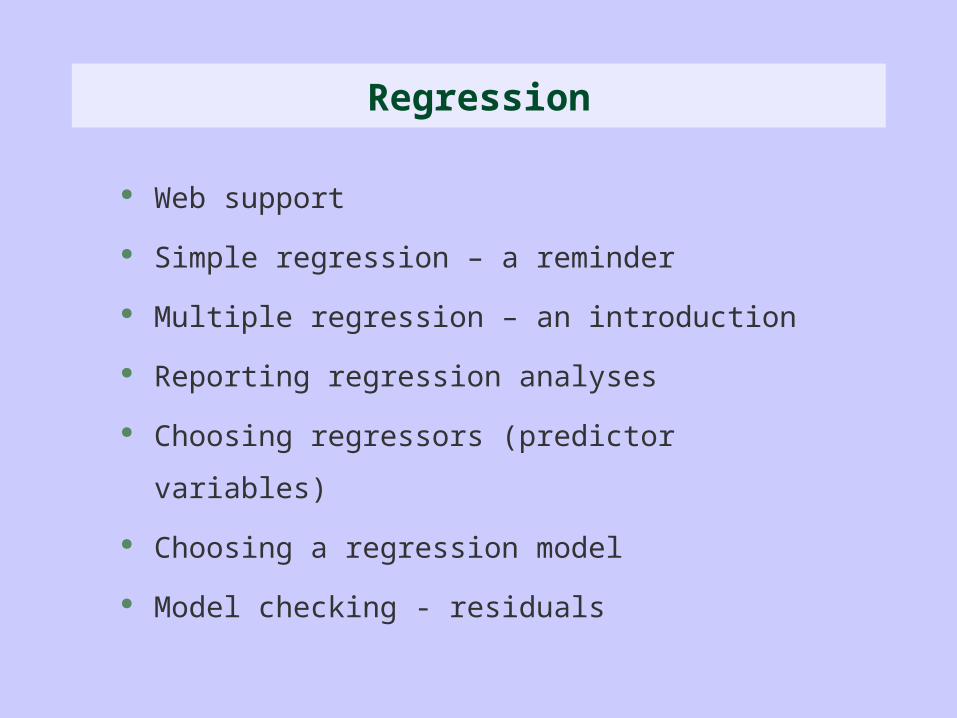
Web support

Simple regression – a reminder

Multiple regression – an introduction

Reporting regression analyses

Choosing regressors (predictor variables)

Choosing a regression model

Model checking - residuals

Regression

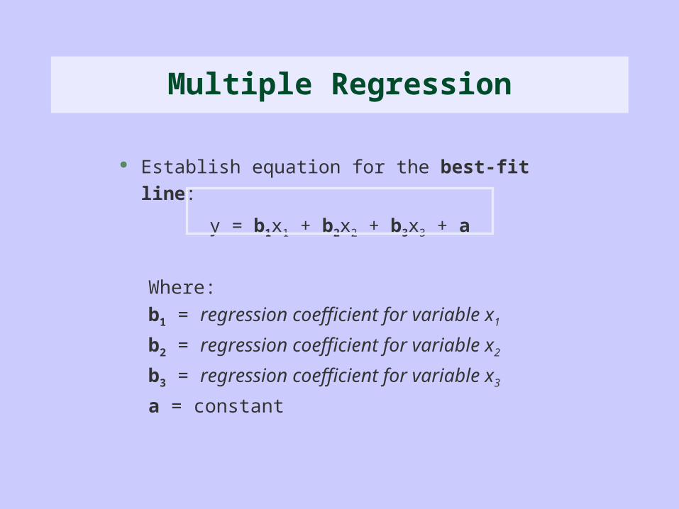
Establish equation for the best-fit line:

y = bx + a

“Best-fit” line same as “Regression” line b is the “regression coefficient” for x x is the “predictor” or “regressor” variable for y

Simple Regression

Establish equation for the best-fit line:

y = b1x1 + b2x2 + b3x3 + a

Multiple Regression

Where:

b1 = regression coefficient for variable x1

b2 = regression coefficient for variable x2

b3 = regression coefficient for variable x3

a = constant

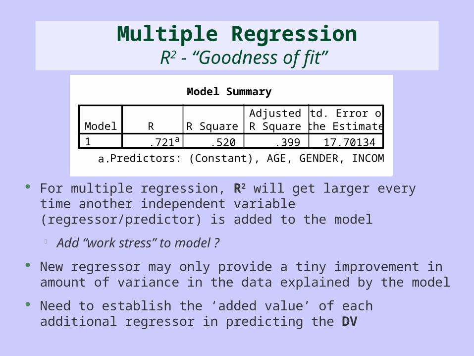
For multiple regression, R2 will get larger every time another independent variable (regressor/predictor) is added to the model

Add “work stress” to model ?

New regressor may only provide a tiny improvement in amount of variance in the data explained by the model

Need to establish the ‘added value’ of each additional regressor in predicting the DV

Multiple Regression R2 - “Goodness of fit”

Model Summary

.721a .520 .399 17.70134Model1

R R SquareAdjustedR Square

Std. Error ofthe Estimate

Predictors: (Constant), AGE, GENDER, INCOMEa.

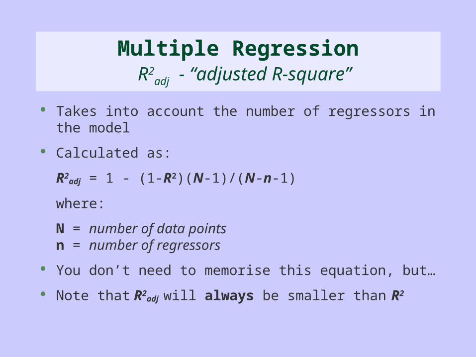
Takes into account the number of regressors in the model

Calculated as:

R2adj = 1 - (1-R2)(N-1)/(N-n-1)

where:

N = number of data pointsn = number of regressors

You don’t need to memorise this equation, but…

Note that R2adj will always be smaller than R2

Multiple Regression R2

adj - “adjusted R-square”

“Effectiveness” vs “Efficiency”

Effectiveness:

maximises R2

ie: maximises proportion of variance explained by model

Efficiency:

maximises increase in R2adj upon adding another regressor

ie: if new regressor doesn’t add much to the variance explained, it is not worth adding

How well does a model explain the variation in the dependent variable?

Effectiveness (R2 and R2adj)

0 - 25% very poor and likely to be unacceptable

25 - 50% poor, but may be acceptable

50 - 75% good

75 - 90% very good

90% + likely that there is something wrong with your analysis

How well does a model explain the variation in the dependent variable?

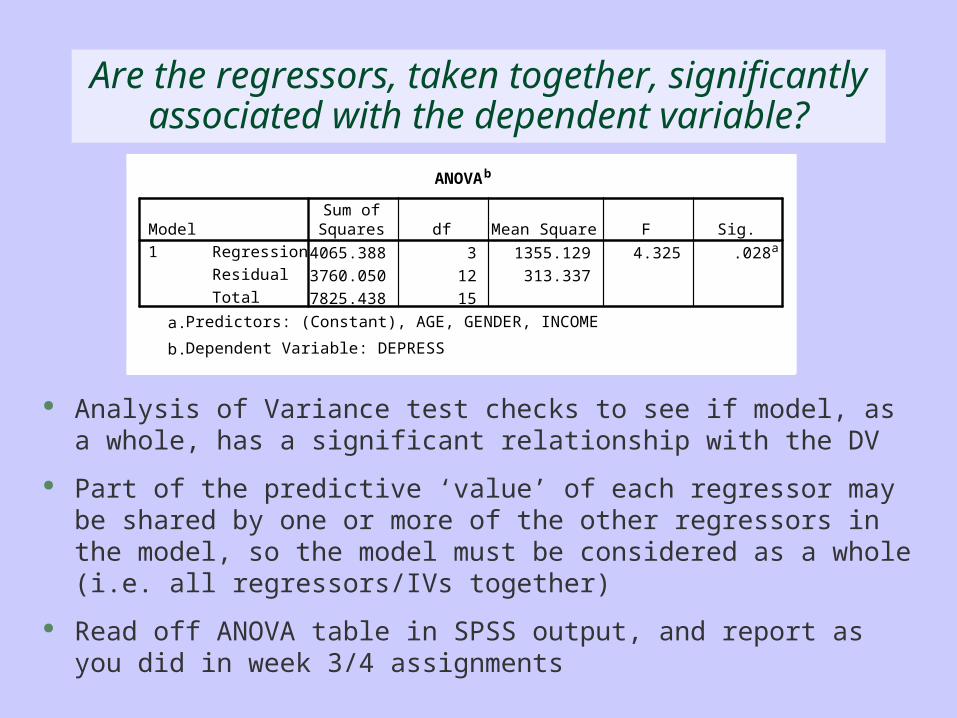
Analysis of Variance test checks to see if model, as a whole, has a significant relationship with the DV

Part of the predictive ‘value’ of each regressor may be shared by one or more of the other regressors in the model, so the model must be considered as a whole (i.e. all regressors/IVs together)

Read off ANOVA table in SPSS output, and report as you did in week 3/4 assignments

Are the regressors, taken together, significantly associated with the dependent variable?

ANOVAb

4065.388 3 1355.129 4.325 .028a

3760.050 12 313.337

7825.438 15

Regression

Residual

Total

Model1

Sum ofSquares df Mean Square F Sig.

Predictors: (Constant), AGE, GENDER, INCOMEa.

Dependent Variable: DEPRESSb.

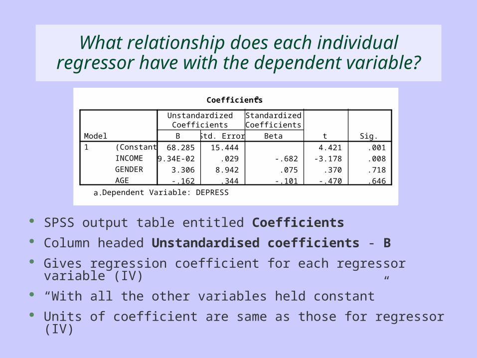
SPSS output table entitled Coefficients Column headed Unstandardised coefficients - B Gives regression coefficient for each regressor variable (IV) “With all the other variables held constant” Units of coefficient are same as those for regressor (IV)

What relationship does each individual regressor have with the dependent variable?

Coefficientsa

68.285 15.444 4.421 .001

-9.34E-02 .029 -.682 -3.178 .008

3.306 8.942 .075 .370 .718

-.162 .344 -.101 -.470 .646

(Constant)

INCOME

GENDER

AGE

Model1

B Std. Error

UnstandardizedCoefficients

Beta

StandardizedCoefficients

t Sig.

Dependent Variable: DEPRESSa.

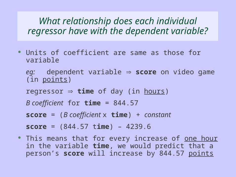
Units of coefficient are same as those for variable

eg: dependent variable score on video game (in points)

regressor time of day (in hours)

B coefficient for time = 844.57

score = (B coefficient x time) + constant

score = (844.57 time) – 4239.6

This means that for every increase of one hour in the variable time, we would predict that a person’s score will increase by 844.57 points

What relationship does each individual regressor have with the dependent variable?

dependent variable score on video game

regressor gender

Gender coded so that: 1 = male, 2 = female

Let B coefficient for gender = 100.00

So, score = 100.00 gender + constant

Adding “1” to the variable gender means that we go from male to female

This means that females would be expected to score 100.00 points more than males

Remember that the B coefficient is calculated on the basis that 1=male and 2=female (different coding will give a different coefficient)

What relationship does each individual regressor have with the dependent variable?

Units for each regression coefficient are different, so we must standardise them if we want to compare one with another

Column headed Standardised coeficients - Beta

Can compare the Beta weights for each regressor variable to compare effects of each on the dependent variable

Larger Beta weight indicates stronger effect of regressor on values of DV

Which regressor has the most effect on the dependent variable?

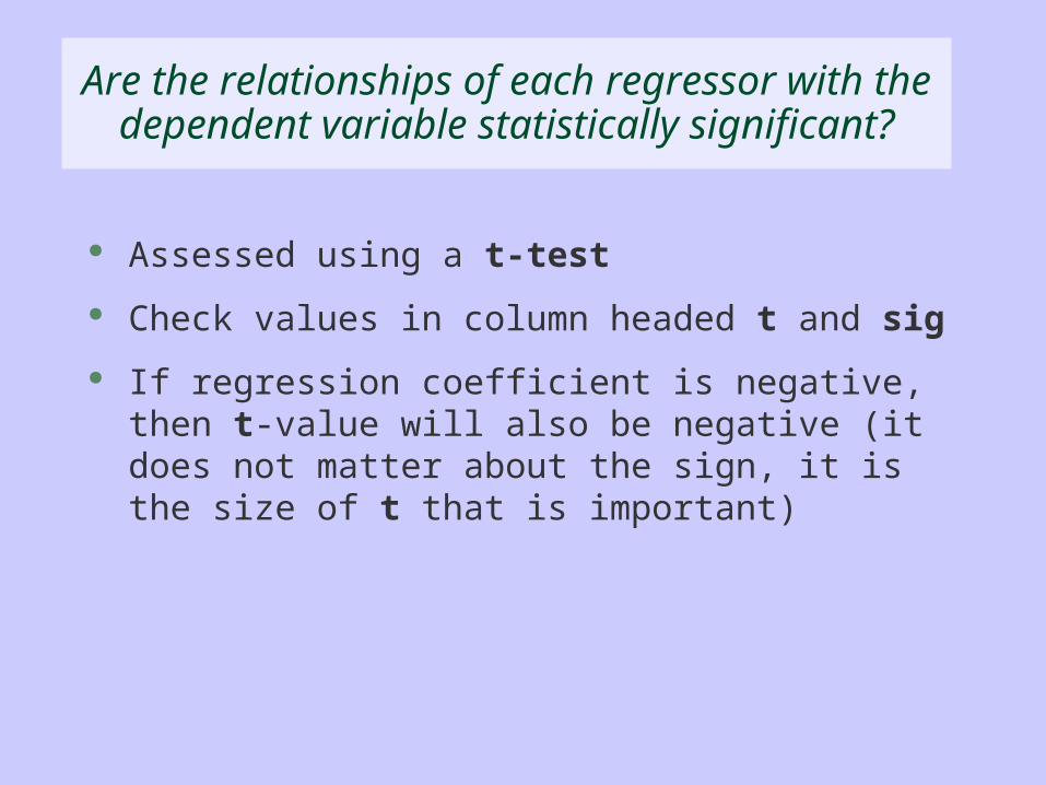
Assessed using a t-test

Check values in column headed t and sig

If regression coefficient is negative, then t-value will also be negative (it does not matter about the sign, it is the size of t that is important)

Are the relationships of each regressor with the dependent variable statistically significant?

How should I report a regression analysis?

Reporting regression analyses

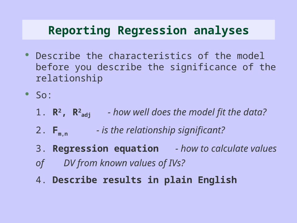
Describe the characteristics of the model before you describe the significance of the relationship

So:

1. R2, R2adj - how well does the model fit the data?

2. Fm,n - is the relationship significant?

3. Regression equation - how to calculate values of

DV from known values of IVs?

4. Describe results in plain English

Reporting Regression analyses

We want to predict IQ score

using brain size (MRI), height and gender as regressors

Units:

IQ: IQ points

brain size (MRI): pixels

height: centimetres

gender: 0 = male, 1 = female

Reporting Regression analyses

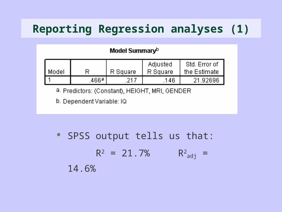
SPSS output tells us that:

R2 = 21.7% R2adj = 14.6%

Reporting Regression analyses (1)

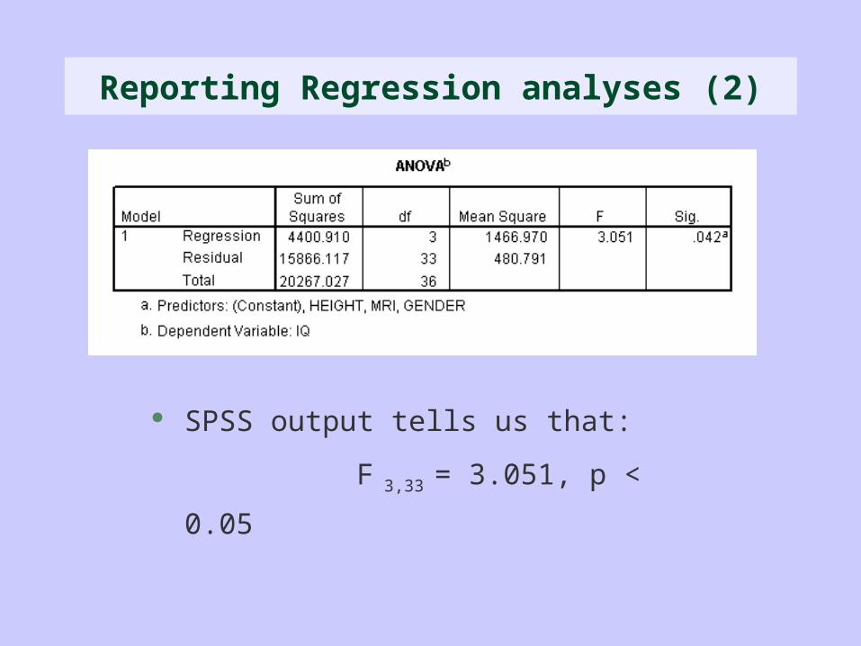
SPSS output tells us that:

F 3,33 = 3.051, p < 0.05

Reporting Regression analyses (2)

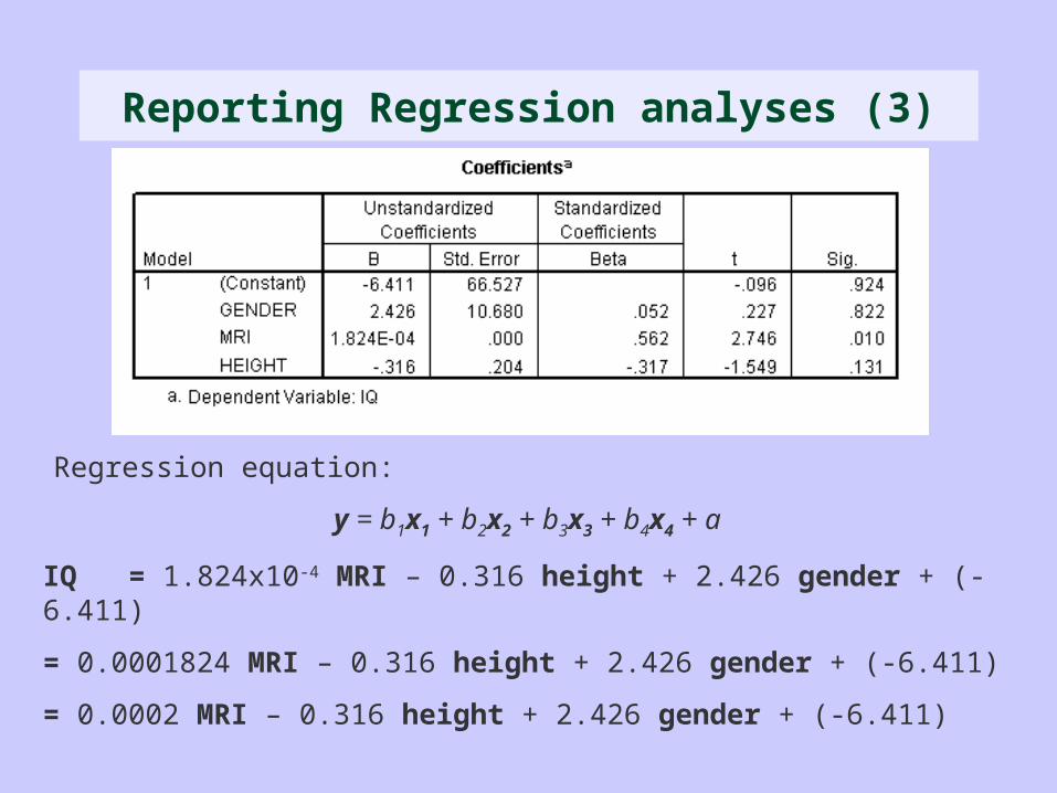
Regression equation:

y = b1x1 + b2x2 + b3x3 + b4x4 + a

IQ = 1.824x10-4 MRI – 0.316 height + 2.426 gender + (-6.411)

= 0.0001824 MRI – 0.316 height + 2.426 gender + (-6.411)

= 0.0002 MRI – 0.316 height + 2.426 gender + (-6.411)

Reporting Regression analyses (3)

“The regression was a poor fit, describing only 21.7% of the variance in IQ (R2

adj= 14.6%), but the overall relationship was statistically significant (F3,33= 3.05, p<0.05).”

“With other variables held constant, IQ scores were negatively related to height, decreasing by 0.32 IQ points for every extra centimetre in height, and positively related to brain size, increasing by 0.0002 IQ points for every extra pixel of the scan. Women tended to have higher scores than men, by 2.43 IQ points. However, the effect of brain size (MRI) was the only significant effect (t33=2.75, p=0.01)”

Reporting Regression analyses (4)

Break

Five minutes – please be back promptly

What do we want of a regressor?

To have ‘a significant effect’ on the dependent variable

Ability to ‘discriminate’ between values of the dependent variable

Selecting Regressors

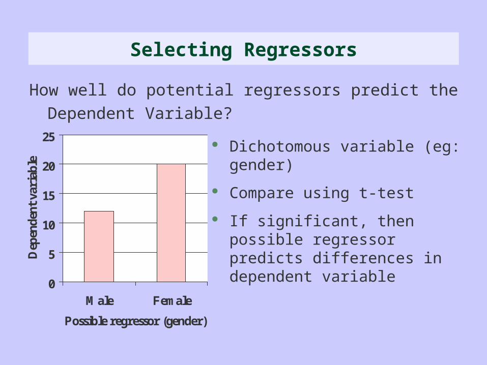
Dichotomous variable (eg: gender)

Compare using t-test

If significant, then possible regressor predicts differences in dependent variable

0

5

10

15

20

25

Male Female

Possible regressor (gender)

Dep

ende

nt v

aria

ble

Selecting Regressors

How well do potential regressors predict the Dependent Variable?

Continuous variable (eg: Height)

Compare using correlation

If significant, then possible regressor predicts differences in dependent variable

0

2

4

6

8

10

12

0 100 200

Possible regressor (height)

Dep

ende

nt v

aria

ble

Selecting Regressors

How well do potential regressors predict the Dependent Variable?

Some of ‘discriminatory value’ in regressor may be accounted for by regressors present in model already

gender, income, height

age, experience, value of property

‘In the presence of all regressors’

Adding regressor may not add as much to model’s predictive value as you might have anticipated

Selecting Regressors

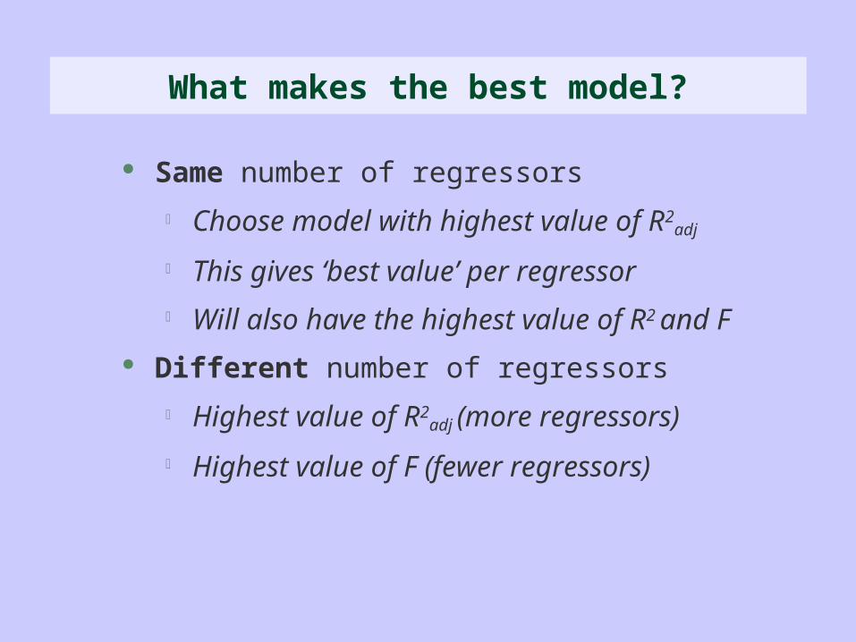
Same number of regressors

Choose model with highest value of R2adj

This gives ‘best value’ per regressor

Will also have the highest value of R2 and F

Different number of regressors

Highest value of R2adj (more regressors)

Highest value of F (fewer regressors)

What makes the best model?

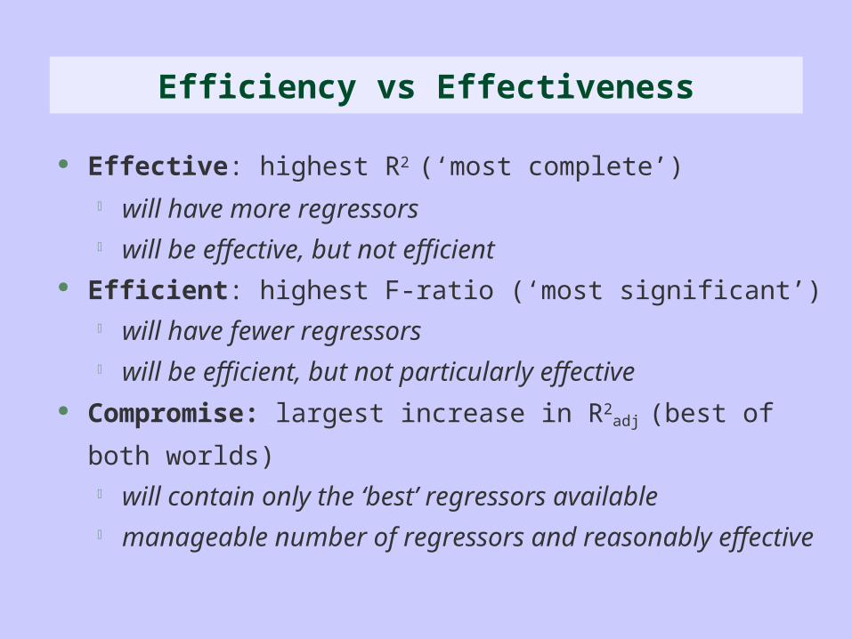
Effective: highest R2 (‘most complete’)

will have more regressors will be effective, but not efficient

Efficient: highest F-ratio (‘most significant’) will have fewer regressors will be efficient, but not particularly effective

Compromise: largest increase in R2adj (best of both worlds)

will contain only the ‘best’ regressors available manageable number of regressors and reasonably effective

Efficiency vs Effectiveness

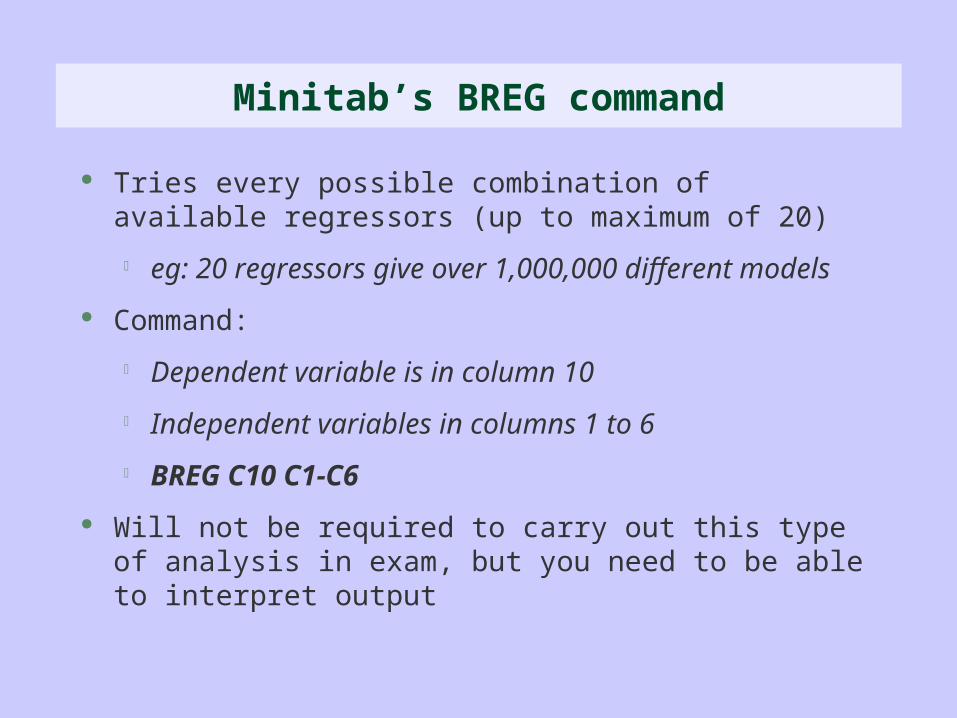
Tries every possible combination of available regressors (up to maximum of 20)

eg: 20 regressors give over 1,000,000 different models

Command:

Dependent variable is in column 10

Independent variables in columns 1 to 6

BREG C10 C1-C6

Will not be required to carry out this type of analysis in exam, but you need to be able to interpret output

Minitab’s BREG command

Sample of BREG outputMTB > BREG C13 C1-C12Best Subsets RegressionResponse is prodebt304 cases used 160 cases contain missing values.

i c c l n h s b b c x o c i i a s m a c m c o h l n a n o a r i a i m o d g g k c n d g s n e u r p e a a a u b b t Adj. g s e a g c c g s u u r Vars R-Sq R-Sq C-p s p e n r p c c e e y y n 7 19.3 17.4 7.3 0.65539 X X X X X X X 7 19.1 17.2 7.8 0.65602 X X X X X X X 8 19.9 17.7 6.9 0.65388 X X X X X X X X 8 19.5 17.4 8.2 0.65536 X X X X X X X X 9 20.2 17.8 7.8 0.65375 X X X X X X X X X 9 20.1 17.6 8.3 0.65434 X X X X X X X X X 10 20.4 17.6 9.3 0.65427 X X X X X X X X X X

Best two models for each possible number of regressors are displayed in output

Compare R2adj values directly

Select best model(s)

Run normal regression in SPSS for each selected model

Compare F-ratio values

BREG output

Identify best subset of regressors from BREG output

Must run ordinary regression procedure

calculates F-ratio

calculates individual coefficients and significance

Highest R2adj values result in significant F-ratios

if F-ratio not significant, check data and procedure

BUT: Advisable to try two or three models, as the number of respondents contributing to each analysis may not be the same between Minitab and SPSS

Best Subset Regression model

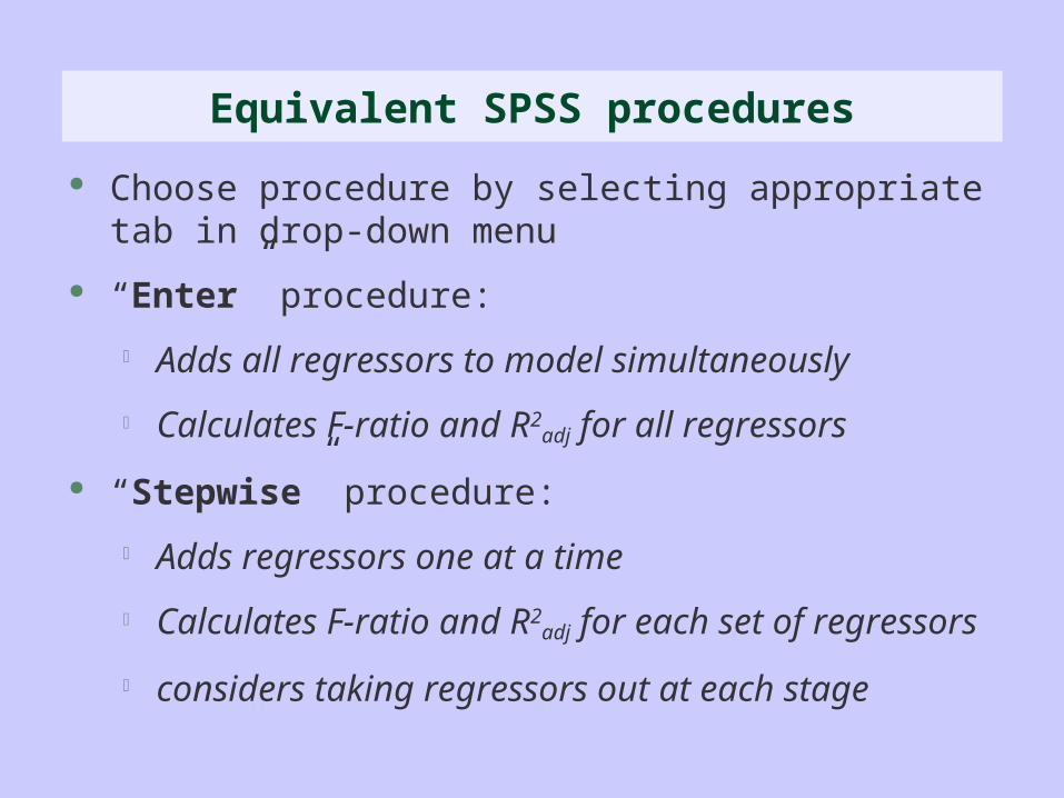
Choose procedure by selecting appropriate tab in drop-down menu

“Enter” procedure:

Adds all regressors to model simultaneously

Calculates F-ratio and R2adj for all regressors

“Stepwise” procedure:

Adds regressors one at a time

Calculates F-ratio and R2adj for each set of regressors

considers taking regressors out at each stage

Equivalent SPSS procedures

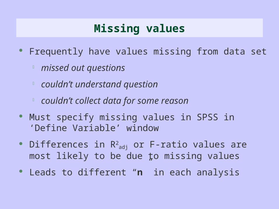
Frequently have values missing from data set

missed out questions

couldn’t understand question

couldn’t collect data for some reason

Must specify missing values in SPSS in ‘Define Variable’ window

Differences in R2adj or F-ratio values are most likely to be due

to missing values

Leads to different “n” in each analysis

Missing values

Residuals (general)

Unusual observations – “outliers”

Model checking

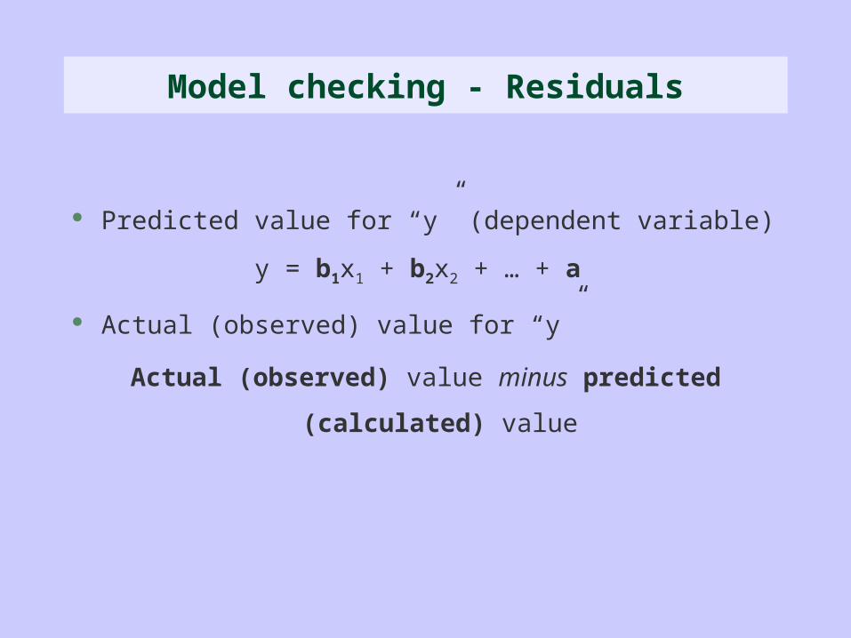
Predicted value for “y” (dependent variable)

y = b1x1 + b2x2 + … + a

Actual (observed) value for “y”

Actual (observed) value minus predicted (calculated) value

Model checking - Residuals

0

20

40

60

80

100

120

140

160

180

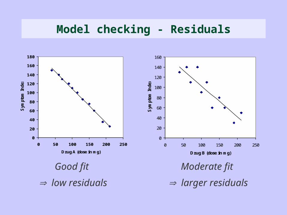
0 50 100 150 200 250

Drug A (dose in mg)

Sym

ptom

In

dex

0

20

40

60

80

100

120

140

160

0 50 100 150 200 250

Drug B (dose in mg)S

ympt

om I

nde

x

Good fit

low residuals

Moderate fit

larger residuals

Model checking - Residuals

Residuals should be:

Normally distributed

some big, some small, most average-sized

Independent of one another

no constant covariation with one another

almost identical in terms of variance

regardless of the values of the IVs or DVs

Model checking - Residuals

These things are easy to check with SPSS ‘plots’ option

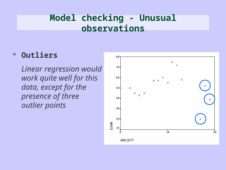
Outliers

Linear regression would work quite well for this data, except for the presence of three outlier points

Model checking - Unusual observations

ANXIETY

20100

EX

AM

80

70

60

50

40

30

20

10

Dealing with outliers

Run regression analysis

Plot data on a scattergram

Remove outliers by deleting the rows in SPSS

Run regression analysis again

Note any qualitative differences:

if there are qualitative differences, then check data. If no errors, report both analyses

if only quantitative differences, then leave outliers in analysis, noting their presence

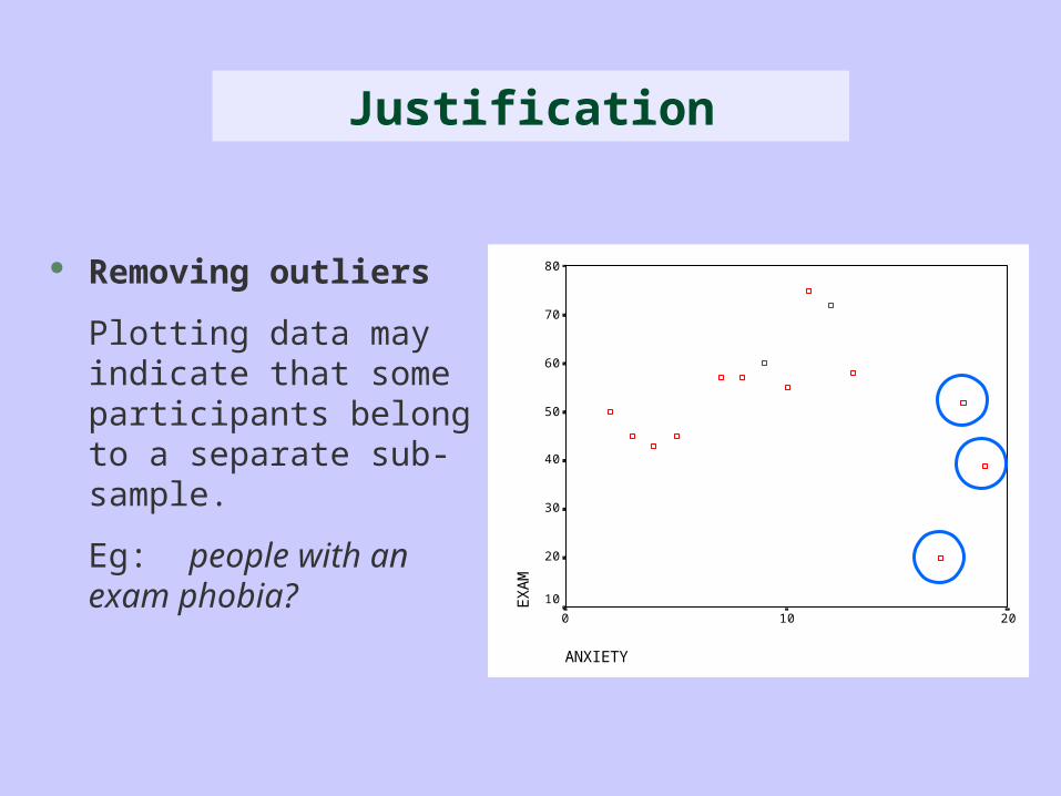
Removing outliers

Plotting data may indicate that some participants belong to a separate sub-sample.

Eg: people with an exam phobia?

Justification

ANXIETY

20100

EX

AM

80

70

60

50

40

30

20

10

ANXIETY

20100

EXAM

80

70

60

50

40

30

20

10

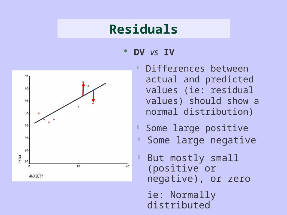
DV vs IV

Differences between actual and predicted values (ie: residual values) should show a normal distribution)

Some large positive

Residuals

Some large negative

But mostly small (positive or negative), or zero

ie: Normally distributed

ANXIETY

20100

EXAM

80

70

60

50

40

30

20

10

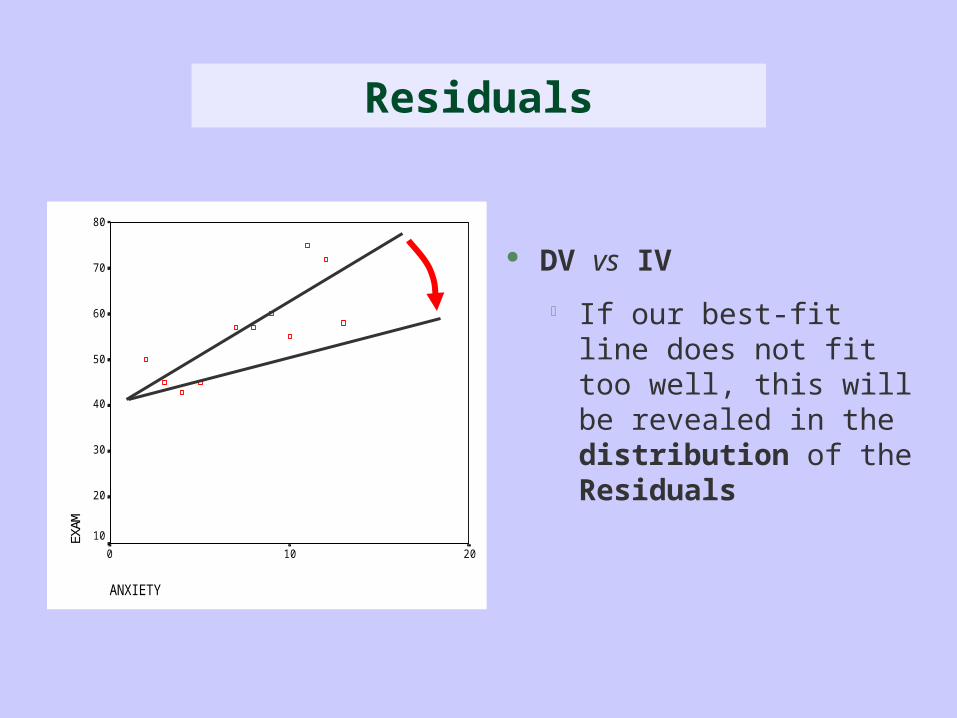
DV vs IV

If our best-fit line does not fit too well, this will be revealed in the distribution of the Residuals

Residuals

Call ……….Veera at 012-2313979

Questions ?