regression testing - department of computer science - allegheny

Regression Testing

Gregory M. KapfhammerDepartment of Computer Science

Allegheny Collegegkapfham�allegheny.eduAppears in theEncyclopedia of Software Engineering(Taylor and Francis)

Keywords:test suite execution, test coverage monitoring, test suiteselection,reduction and prioritization, efficiency and effectiveness trade-offs

Abstract. Regression testing techniques execute a test suite whenever the addition ofdefect fixes or new functionality changes the program under test. The repeated exe-cution of a test suite aims to establish a confidence in the correctness of the softwareapplication and identify defects that were introduced by the program modifications.Industry experiences suggest that regression testing often improves the quality of theapplication under test. However, testing teams may not always perform regressiontesting because the frequent execution of the tests often incurs high time and spaceoverheads. Test suiteselectiontechniques try to reduce the cost of testing by runninga subset of the tests, such as those that execute the modified source code, in order toensure that the updated program still operates correctly. Alternatively,reductionmeth-ods decrease testing time overheads by discarding the teststhat redundantly cover thetest requirements. Approaches to test suiteprioritization reorder the test cases in anattempt to maximize the rate at which the tests achieve a testing goal such as codecoverage. After describing a wide variety of metrics for empirically evaluating differ-ent regression testing methods, this chapter considers theefficiency and effectivenesstrade-offs associated with these techniques. The conclusion of this article summarizesthe state-of-the-art in the field of regression testing and then offers suggestions forfuture work and resources for further study.

1 INTRODUCTION

Regression testing is an important software maintenance activity that involves repeatedly run-ning a test suite whenever the program under test and/or the program’s execution environmentchanges. Executing a regression test suite upon the introduction of either a defect fix or a newfeature ensures that the modification of the program does notnegatively impact the overall cor-rectness. Recent industry reports suggest that (i) software engineers often use regression testingtechniques [1] and (ii) employing regression testing methods often leads to a software applica-tion with high observed quality [2]. However, regression testing can be prohibitively expensive,particularly with respect to time [3], and thus accounts foras much as half the cost of softwaremaintenance [4, 5]. In Rothermel et al. [5], an industrial collaborator reported that for one of itsproducts of approximately 20,000 lines of code, the entire test suite required seven weeks to run.

INTRODUCTION Author: Kapfhammer 2

Since several well-known software failures, such as the Ariane-5 rocket and the 1990 AT&T out-age, can be blamed on not testing changes in a software system[6], many techniques have beendeveloped to support efficient and effective regression testing. For instance, atest suite execution(TSE) component (e.g., JUnit, CppUnit, or NUnit) runs a large test suite in an automated andrepeatable manner. As the test suite executes, atest coverage monitor(TCM) tracks how the testcases cover the test requirements that normally correspondto the program’s state or structure(e.g., methods, statements, or definition-use associations). Whenever coverage information isavailable, reduction, prioritization, and selection algorithms can analyze the relative contributionof each test case in order to improve the regression test suite.

Regression test suitereductiontechniques aim to control both the size and the execution time ofa test suite by discarding the tests that redundantly cover the test requirements. In an attempt toimprove the effectiveness of testing, approaches to test suite prioritization reorder the test casesaccording to an established priority metric. For instance,the prioritizer may rearrange the testsso that they cover the test requirements at a faster rate thanthe original ordering. Alternatively,a test prioritization method may addresses the challenge ofrunning a test suite in a constrainedenvironment where computational resources such as time andmemory are limited. Test suiteselectiontechniques try to reduce the cost of testing by only running those test cases that are mostlikely to ensure that the modified program still operates correctly (e.g., the tests that exercise themodified source code of the program).

There are many costs and benefits associated with the regression testing process. Both practi-tioners and researchers must conduct experiments in order to ascertain the trade-offs betweenthe efficiency and the effectiveness of the chosen method(s)for regression testing. For instance,it is important to measure the time overhead associated withexecuting the tests and monitoringthe coverage of the requirements. Experiments must also determine the time and space costsof using a selection, reduction, or prioritization algorithm and then evaluate these overheads inthe context of the potentially diminished cost and increased effectiveness of the modified testsuite. For example, the empirical characterization of a reduction technique frequently measuresthe decrease in the size and execution time of the test suite [7, 8], preservation of the originaltest suites’ coverage [8, 9], or the amount of tests that are found in common for test suites pro-duced by different reduction methods [10]. After characterizing the coverage density of a testsuite [11], experimental studies of test prioritization schemes typically focus on evaluating thechange in metrics such as coverage effectiveness (CE) [9], average percentage of blocks covered(APBC) [12], and average percentage of faults detected (APFD) [4, 13].

In summary, the important contributions of this chapter areas follows:

1. An overview of a model for the regression testing process (Section 2.1).

2. A description of the reduction, prioritization, and selection techniques that are often usedduring regression testing (Sections 2.2 through 2.7).

3. The definition of the metrics that evaluate the efficiency and effectiveness of differentapproaches to regression testing (Section 3).

4. A review of the important advances and the current state ofthe art in the field of regressiontesting (Sections 4 and 5).

REGRESSION TESTING TECHNIQUES Author: Kapfhammer 3

Begin Coverage Report End

VSRT RepeatProgram

Selection, Reduction, or Prioritization

Original Test Suite

Modified Test Suite

Test Suite Execution

Testing Results

GRT Repeat

GRT - General Regression TestingVSRT - Version Specific Regression Testing

Figure 1: Overview of the Regression Testing Process.

2 REGRESSION TESTING TECHNIQUES

2.1 REGRESSION TESTING MODEL

Figure 1 provides an overview of a model for the regression testing process. In thegeneralre-gression testing (GRT) framework, we apply selection, reduction, and/or prioritization to the testsuite and then use the modified suite during many subsequent rounds of test suite execution [5].This cost-effective approach to testing is motivated by empirical studies demonstrating that theadequacy of a test suite does not markedly change across subsequent versions of a program [14].Alternatively, theversion specificregression testing (VSRT) model suggests that the test suiteshould be re-analyzed after each modification to the programunder test [5]. VSRT requires effi-cient implementations of the (i) test suite executor, (ii) test coverage monitor, and (iii) selection,reduction, and prioritization techniques. If the method for constructing the modified test suite isexpensive, then the GRT framework supports the amortization of this cost over many executionsof the tests. Yet, VSRT is more likely to improve the effectiveness of regression testing becauseit always leverages the most current information about the program and the tests. Furthermore,testers should consider the VSRT approach whenever the program and/or the test suite undergoa series of substantial changes. Of course, any regression testing approach that can efficientlyoperate in a version specific fashion should also enable GRT.

Regression testing establishes a confidence in the correctness of and isolates defects within aprogram by running a collection of tests known as atest suite. This chapter defines a test suiteT = 〈t1, . . . , tn〉 as a tuple (i.e., an ordered list) ofn individual test cases. Intuitively, each testcaseti ∈ T invokes one or more of the methods under test and inspects theoutput(s) in orderto see if the operations worked correctly. We require that each test inT be independentso thatwe can guarantee that there are no test execution ordering dependencies [4, 15]. Many realworld test suites exhibit test independence because the most popular test automation frameworks(e.g., JUnit, CppUnit, or NUnit) providesetUp andtearDown methods that respectively executebefore and after each test case. Test case independence alsomakes it more likely that regressiontesting schemes (e.g., selection, reduction, and prioritization) will create a modified test suitethat is both efficient and effective. For instance, test independence enables a prioritizer to reordertests in any sequence that maximizes the suite’s ability to cover the test requirements and find

2.2 TEST SUITE EXECUTION Author: Kapfhammer 4

Input 2 - Method Under Test

Output 3 - Test Oracle

Expected Output

Verdict

1 - Set Up

4 - Tear Down

Figure 2: Overview of the Test Suite Execution Process.

the defects. All of the testing techniques described in thischapter may also be applied, albeit ina potentially diminished capacity, to non-independent regression test suites.

2.2 TEST SUITE EXECUTION

Figure 2 describes the process of executing a test case. As previously mentioned in Section 2.1,a setUp operation runs before the invocation of the method under test in order to perform anyrequired initializations. For example, if the program interacts with a file system or a database,then setUp may populate these components with files or data. Alternatively, if the programuses a network, thensetUp could establish a new network connection. Upon completion ofthe initialization procedure, the test case calls the program’s method with the input that the testconstructs. The test case captures the output of the method and provides the return value to thetest oraclethat determines whether the test passed or failed.

While tools may automatically generate oracles in certain circumstances (e.g., when it is possibleto predict the output of new tests based upon the input and output of existing test cases [16]),often the tester manually implements the oracles. The oracle returns a failing verdict when theexpected output does not match the actual output and a passing verdict results when the twooutputs are equivalent. Finally,tearDown cleans up after the test case and thus ensures that itis independent. Depending on the configuration of the test suite executor, the regression testingprocess continues until either all of then tests have executed or an oracle indicates that a test casefailed (this behavior is the default for most versions of theJUnit test automation framework).

In order to make the discussion of test suite execution more concrete and to illustrate the chal-lenges of testing, Figure 3 summarizes the outcomes associated with testing a Java class calledKineti [4]. As shown in Figure 4, this class contains a omputeVelo ity method designedto calculate the velocity of an object based on its kinetic energy and mass. Since the kineticenergy of an object,K, is defined asK = 1

2mv2, it is clear that omputeVelo ity contains adefect on line 10. That is, line 10 should have the assignmentstatementvelo ity_squared= 2 * (kineti / mass). Furthermore, Figure 5 gives a test suite that will run in theJUnit3.8.1 framework for automated test execution (a slightly modified version of this suite will fullfilthe requirements of the more recent 4.8.1 version of JUnit).Interestingly, the results in Figure 3reveal that only one of the four tests,t4, reveals the fault in theKineti class.

2.3 TEST ADEQUACY CRITERIA Author: Kapfhammer 5

Test Case kineti mass expe ted a tual VerdicttestOne - t1 5 0 Undefined Undefined PasstestTwo - t2 0 5 0 0 PasstestThree - t3 8 1 4 4 PasstestFour - t4 1000 5 20 24 Fail

Figure 3: Summarizing the Outcomes of Test Suite Execution for omputeVelo ity.

For instance,t1 cannot isolate the fault in omputeVelo ity because it does not executeline 10 of the program. Testt2 is also incapable of detecting the defect since an input ofkineti = 0 results invelo ity_squared = velo ity = final_velo ity = 0 and thusleads to an inadvertently passing test case. Testt3 passes even after the method incorrectly as-signsvelo ity_squared = 24 and subsequently computesMath.sqrt(velo ity_squared)= 4.898979 instead of the correct value ofMath.sqrt(velo ity_squared) = 4.0. Testt3’sinability to find the defect is due to the fact that line 11 of omputeVelo ity masks the faultycomputation by casting thevelo ity variable as anint and arriving at the expected result ofvelo ity = 4. Yet, Figure 3 shows thatt4 is capable of isolating the defect because it executesthe faulty location, changes the value of thefinal_velo ity variable, and returns the incorrectresult to the calling test case. In summary, this example demonstrates that tests often do not havethe same fault detection effectiveness. We also see that a program fault only manifests itself ina test failure when the input(s) (i) cause the execution of the defective location, (ii) change thevalues of the program’s variables, and (iii) force the method to return an erroneous answer [17].It is also evident that an effective regression testing process must use a test suite executor that can(i) repeatedly run the test cases, (ii) capture the output ofthe method under test, and (iii) issue afinal verdict after using an oracle to compare the value of theexpe ted anda tual variables.

2.3 TEST ADEQUACY CRITERIA

Ideally, a regression testing technique would utilize knowledge about program faults as it re-ordered and reduced the test cases. Since it is normally difficult to collect information about theexistence of faults within the program under test, regression testing methods must use a proxyfor this type of complete knowledge. After identifying a type of test requirement that “good”test cases should aim to exercise, testers can calculate theadequacyof a test case as the ratio be-tween the covered requirements and the total number of requirements. For example, a criterionthat concentrates on thecontrol flowof the program under test does so with the realization that adefect cannot be detected unless the test case executes the faulty location in the program’s sourcecode. Alternatively, adata flowadequacy criterion focuses on the definition and use of variablesbecause a program will only be able to determine if it assigned the correct value to a variablewhen it subsequently uses the variable. An adequacy criterion could also consider the coverageof the program’s methods and the context in which the methodswere invoked during testing.

Current regression testing methods are often motivated by empirical investigations of the effec-tiveness of test adequacy criteria which indicate that the low adequacy tests are often unlikelyto reveal program defects [18]. If adequacy information is available, then a test prioritizer couldexecute highly adequate tests before those with lower adequacy. As a concrete illustration ofthe concept of test adequacy, this chapter briefly examines criteria that focus on definition-use


1 import j a v a . lang . Math ;2 p u b l i c c l a s s K i n e t i c3 {4 p u b l i c s t a t i c S t r i n g com pu teVe loc i t y (i n t k i n e t i c , i n t mass )5 {6 i n t v e l o c i t y _ s q u a r e d , v e l o c i t y ;7 S t r i n g B u f f e r f i n a l _ v e l o c i t y = new S t r i n g B u f f e r ( ) ;8 i f ( mass != 0 )9 {

10 v e l o c i t y _ s q u a r e d = 3∗ ( k i n e t i c / mass ) ;11 v e l o c i t y = (i n t ) Math . s q r t ( v e l o c i t y _ s q u a r e d ) ;12 f i n a l _ v e l o c i t y . append ( v e l o c i t y ) ;13 }14 e l s e15 {16 f i n a l _ v e l o c i t y . append ( " Undef ined " ) ;17 }18 return f i n a l _ v e l o c i t y . t o S t r i n g ( ) ;19 }20 }

Figure 4: TheKineti Class that Contains a Fault in the omputeVelo ity Method.

1 import j u n i t . f ramework .∗ ;2 p u b l i c c l a s s T e s t K i n e t i c extends TestCase3 {4 p u b l i c T e s t K i n e t i c ( S t r i n g name )5 {6 super ( name ) ;7 }8 p u b l i c s t a t i c T es t s u i t e ( )9 {

10 return new T e s t S u i t e ( T e s t K i n e t i c .c l a s s ) ;11 }12 p u b l i c vo id t e s t O n e ( )13 {14 S t r i n g expec ted =new S t r i n g ( " Undef ined " ) ;15 S t r i n g a c t u a l = K i n e t i c . com pu teVe loc i t y ( 5 , 0 ) ;16 a s s e r t E q u a l s ( expected , a c t u a l ) ;17 }18 p u b l i c vo id tes tTwo ( )19 {20 S t r i n g expec ted =new S t r i n g ( " 0 " ) ;21 S t r i n g a c t u a l = K i n e t i c . com pu teVe loc i t y ( 0 , 5 ) ;22 a s s e r t E q u a l s ( expected , a c t u a l ) ;23 }24 p u b l i c vo id t e s t T h r e e ( )25 {26 S t r i n g expec ted =new S t r i n g ( " 4 " ) ;27 S t r i n g a c t u a l = K i n e t i c . com pu teVe loc i t y ( 8 , 1 ) ;28 a s s e r t E q u a l s ( expected , a c t u a l ) ;29 }30 p u b l i c vo id t e s t F o u r ( )31 {32 S t r i n g expec ted =new S t r i n g ( " 20 " ) ;33 S t r i n g a c t u a l = K i n e t i c . com pu teVe loc i t y ( 1 0 0 0 , 5 ) ;34 a s s e r t E q u a l s ( expected , a c t u a l ) ;35 }36 }

Figure 5: A JUnit 3.8.1 Test Suite for the FaultyKineti Class.


4

6

1def(x)

2use(x)use(y)

def(y)

3use(x)

use(x)use(y)def(x)

use(x)use(y)def(y)

use(x)use(y)

exitm

5

use(y)

menter

FT

Figure 6: Example of a Graph-Based Representation for a Simple Program Under Test.

associations [19] and call tree paths [7, 8]. Data flow-basedcriteria are frequently very effectivebecause they consider both the values stored in the program’s variables and the structure of theprogram itself. Since data flow-based adequacy criteria often require the use of a potentiallyexpensive algorithm to enumerate the definition-use associations, these criteria may not supportthe version specific model of regression testing [9, 20]. Furthermore, it is difficult to apply dataflow criteria to programs for which testers lack access to thesource code. Alternatively, thischapter considers call tree paths, a efficient-to-compute criterion that operates without sourcecode access by focusing on the contextual coverage of the methods invoked during testing.

In data flow-based adequacy criteria, the occurrence of a variable on the left hand side of anassignment statement is called adefinitionof this variable. Theuseof a variable takes place whenit appears on the right hand side of an assignment statement or in the predicate of a conditionallogic statement or an iteration construct [18]. For example, the assignment statementx = x + yuses the variablesx andy and then definesx. Figure 6 furnishes an intuitive depiction of a graph-based representation for a method under test. In this diagram, a node represents a computationand an edge stands for the transfer of control between two separate statements within the program[4]. The node labeled with a “4” in Figure 6, denoted here asN4, would represent the definitionand uses of program variables for the statementx = x + y.

A data flow-based adequacy criterion calledall-DUs requires a test suite to cover adefinition-useassociation〈Nd,Nu,var〉 where the definition of variablevar occurs in graph nodeNd and a useof var occurs in nodeNu [18]. For instance, the coverage report in Figure 7 reveals that〈N1,N4,x〉is one of the sixteen definition-use associations within thegraph provided by Figure 6. Figure 7also shows that a test case exercising the pathN1→N2→N3→N4→N6 will cover seven of theassociations and thus lead to an adequacy score of.4375. Yet, we see that a test case that alsofollows the edgeN4→N2 will increase its measure of adequacy to.5625. Various approaches toregression testing use data flow information, such as the definition-use associations described inFigure 7, during the reorganization of a test suite. For example, a prioritizer may order the suiteso that the first tests to run have the highest data flow adequacy.


R1 = 〈N1,N2,x〉R2 = 〈N1,N2,y〉R3 = 〈N1,N3,x〉R4 = 〈N1,N3,y〉R5 = 〈N1,N4,x〉R6 = 〈N1,N4,y〉R7 = 〈N1,N5,x〉R8 = 〈N1,N5,y〉

R9 = 〈N4,N2,x〉R10 = 〈N5,N2,y〉R11 = 〈N5,N3,y〉R12 = 〈N4,N3,x〉R13 = 〈N4,N6,x〉R14 = 〈N5,N6,y〉R15 = 〈N4,N5,x〉R16 = 〈N5,N4,y〉

Path Covered Associations Adequacy

N1→N2→N3→N4→ N6 R1, R2, R3, R4, R5, R6, R13716 = .4375

N1 → N2 → N3 → N4 →N2→N3→N4→N6

R1, R2, R3, R4, R5, R6, R9, R12, R13916 = .5625

Figure 7: Test Requirements for theall-DUs Adequacy Criterion.

Alternatively, McMaster and Memon present a test adequacy criterion that obviates the need forsource code access by measuring method coverage in the context in which the methods wereinvoked during testing [7]. A coverage report for this criterion corresponds to either adynamiccall tree(DCT) or acalling context tree(CCT) representing the dynamic behavior of the programwhile a test suite runs. Each node in a DCT or CCT stands for a method that was called duringthe execution of a test case. An edge from a parent to a child node signifies that the parent methodcalled the child method during testing. Finally, a call treepath from the root node to a leaf nodeforms a test requirement. Regression testing methods may use call tree paths as a test adequacycriterion because these trees are efficient to collect and store, thus enabling the modification of atest suite each time the program under test changes [9, 21]. Although DCTs and CCTs may becriticized for not incorporating either the source code or parameters of the methods under test orthe state of the program, they have been shown to perform closely to other criteria with respectto common fault detection metrics [22].

Figure 8(a) provides an example of a DCT with thirteen nodes and twelve edges. In this treea node with the label “A” corresponds to the invocation of themethod A and the edge A→B indicates that method A invokes method B. The existence of the two DCT edges A→ Breveals that method A repeatedly invokes method B. In the example from Figure 8(a), the DCTrepresents the recursive invocation of method G by chainingtogether edges of the form G→ G.In an attempt to reduce the size of the coverage report, the CCT in Figure 8(b) coalesces the DCTnodes and yields a 30.8% reduction in the number of nodes and a 16.7% decrease in the numberof edges. For example, the CCT combines the two B nodes in the DCT into a single node. TheCCT also coalesces nodes and introduces back edges when a method calls itself recursively (e.g.,the DCT path G→ G→ G) or a method is run repeatedly (e.g., the DCT path H→ I → H).

Using call tree paths as a test requirement enables regression testing techniques to determinewhich test cases may be redundant [7]. For instance, comparing a test that only causes method

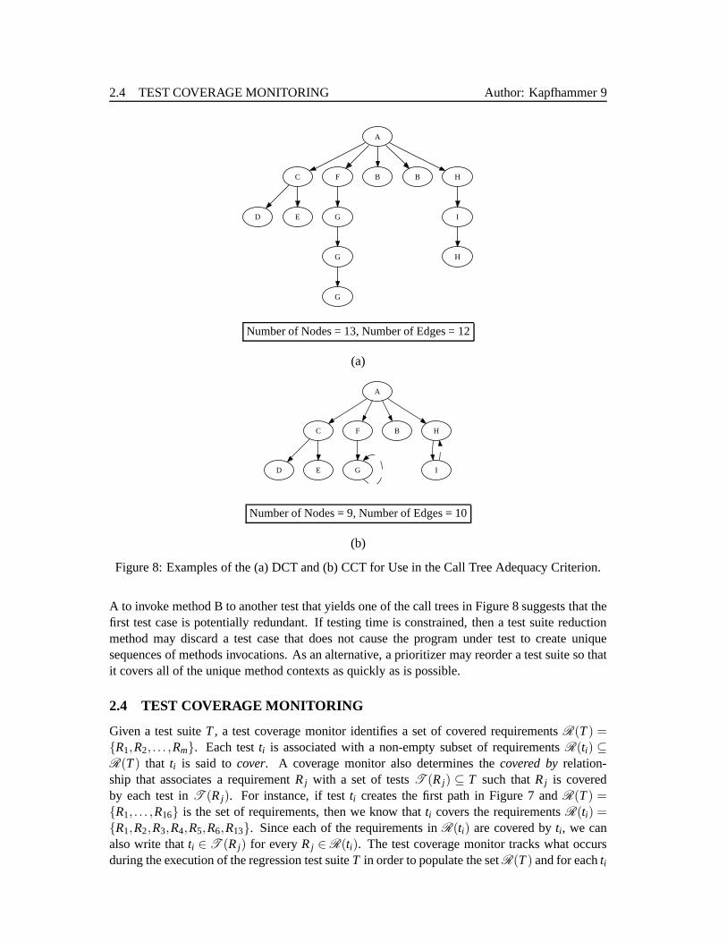
2.4 TEST COVERAGE MONITORING Author: Kapfhammer 9

A

C F B B H

D E G

G

G

I

H

Number of Nodes = 13, Number of Edges = 12

(a)

A

C F B H

D E G I

Number of Nodes = 9, Number of Edges = 10

(b)

Figure 8: Examples of the (a) DCT and (b) CCT for Use in the CallTree Adequacy Criterion.

A to invoke method B to another test that yields one of the calltrees in Figure 8 suggests that thefirst test case is potentially redundant. If testing time is constrained, then a test suite reductionmethod may discard a test case that does not cause the programunder test to create uniquesequences of methods invocations. As an alternative, a prioritizer may reorder a test suite so thatit covers all of the unique method contexts as quickly as is possible.

2.4 TEST COVERAGE MONITORING

Given a test suiteT, a test coverage monitor identifies a set of covered requirementsR(T) ={R1,R2, . . . ,Rm}. Each testti is associated with a non-empty subset of requirementsR(ti) ⊆R(T) that ti is said tocover. A coverage monitor also determines thecovered byrelation-ship that associates a requirementRj with a set of testsT (Rj) ⊆ T such thatRj is coveredby each test inT (Rj). For instance, if testti creates the first path in Figure 7 andR(T) ={R1, . . . ,R16} is the set of requirements, then we know thatti covers the requirementsR(ti) ={R1,R2,R3,R4,R5,R6,R13}. Since each of the requirements inR(ti) are covered byti, we canalso write thatti ∈ T (Rj) for everyRj ∈R(ti). The test coverage monitor tracks what occursduring the execution of the regression test suiteT in order to populate the setR(T) and for eachti

2.4 TEST COVERAGE MONITORING Author: Kapfhammer 10

Start Testing

Before Probe

End Testing

Continue Testing

Call Tree Storage

Call Tree

Call Tree

Update

Method or Test Invocation

After Probe

Update

Call Tree Initialization

Figure 9: Call Tree Construction Probes for Test Coverage Monitoring.

andRj construct the respective setsR(ti) andT (Rj). Test coverage monitoring techniques placeinstrumentationprobesinto the program under test in order to report which test requirements arecovered during the execution ofT. Among other goals, the instrumentation must efficiently trackcoverage without changing the behavior of the program and the test suite [9, 20, 21].

This chapter primarily uses the call tree path coverage criterion to support the discussion of theinstrumentation and test coverage monitoring process. As shown in Figure 9, the use of calltree-based test adequacy requires probes to execute beforeand after the execution of both a testcase and a method. Each time a probe executes, it must update the call tree so that it correctlyreflects the test execution history and eventually results in a tree like the ones in Figure 8. Sincethese probes do not initially exist in the program under test, the coverage monitor must placethem into the methods of the program. Using aspect-orientedprogramming (AOP) techniquesand tools such as AspectJ, a call tree constructor inserts instrumentation probes in either a staticor dynamic fashion [8, 21]. Astatic instrumentor places the probes into the program beforetest suite execution whereasdynamicinstrumentation methods insert the probes as the tests run.While static instrumentation must take place each time the program under test changes, dynamicinstrumentors modify the program during testing, thus improving the flexibility of the monitor atthe cost of a potential increase in run-time overheads.

As an example, test coverage monitors for Java programs can use either the Java virtual machinetools interface (JVMTI) or a custom class loader in order to perform dynamic instrumentation atclass load-time [9]. While this approach is simple and easy to implement, it may insert probesthat are not necessary and it cannot support the gathering ofinformation for certain types ofadequacy criteria (e.g., definition-use associations for program variables). Alternatively, Misurdaet al. present the Jazz test coverage monitor that records information about the execution ofcontrol flow-based (e.g., edges and nodes) and data flow-based (e.g., definition-use associations)test requirements [20]. While more complicated than the useof AspectJ to construct call trees,this instrumentation scheme is unique because it incrementally removes the probes after a testcase exercises the associated test requirements. In summary, instrumentation methods vary intheir ability to capture various aspects of program behavior and they are commonly tailored totrack the coverage of requirements for one or more specific test adequacy criteria.

2.5 REDUCING AND PRIORITIZING TEST SUITES Author: Kapfhammer 11

t1

R1

t2 t3t4 t5

R5

t6t7

R2

t8 t9

R6

t10

R7

t11

R4

t12

R3

ti → Rj means that testti coversrequirementRj

Figure 10: An Example of Overlap in the Coverage of the Test Requirements.

2.5 REDUCING AND PRIORITIZING TEST SUITES

Figure 10 visualizes a coverage report that a coverage monitor constructed after running a testsuiteT consisting of tests〈t1, . . . , t12〉 and requirementsR(T) = {R1, . . . ,R7}. Using the nota-tion established in Section 2.4, this example illustrates coverage relationships such asR(t1) ={R1,R4} andT (R1) = {t1, t2}. Since the test suite in Figure 10 contains a significant amount ofoverlap in test requirement coverage, it is a candidate for reduction. In fact, inspection of Fig-ure 10 reveals that executing a reduced test suite containing 〈t2, t3, t6, t9〉 instead of the originaltwelve tests will still cover all of the seven test requirements (other reductions are also possi-ble for this test suite). Even though test suite reduction maintains complete coverage of therequirements, it does not guarantee the same fault detection capabilities as the original test suite[7, 22, 23]. If a tester is concerned that test suite reduction might compromise the fault detec-tion effectiveness of the suite, then it may be reasonable toreorder the tests. For instance, atest suite prioritizer could construct a test sequence thatruns the high coverage test cases (i.e.,R(t10) = {R4,R6,R7}) before the tests that cover few requirements (i.e.,R(t12) = {R3}).

Reduction methods attempt to produce a new test suite that issmaller than the input test suiteT.While reducers ignore the redundant tests, a prioritizer repeatedly inputs the surplus tests intothe reduction algorithm until all of the tests have been added to a completely reordered suite.As shown in Figure 11, it is possible to prioritize a test suite by repeatedly invoking a reductionalgorithm on successively smaller subsets of the tests [8].Given a test suiteT and test cover-age setR(T) as input, thePrioritizationViaRepeatedReductionalgorithm initializesTp to theempty set and assignsR(T) as the set of live requirementsRℓ(T). While there are still testsremaining inT, the algorithm repeatedly uses a reduction technique, suchas theGreedyReduc-tionWithOverlapalgorithm described in Section 2.5.1, to find a reduced suiteTr . Each iterationof the loop starting on line 2 of Figure 11 uses the order preserving union operator, denoted⊎,to add the tests from the resultingTr to Tp and then recalculates the live requirementsRℓ(T).

Figure 12 furnishes an example of this process for the small test suite that is provided to the rightof the diagram. The checkmarks in this coverage report reveal that t1 covers four requirements(i.e.,R1,R2,R3, andR4) while test caset4 covers only two requirements (i.e.,R1 andR4). Whengiven the original test suiteT = 〈t1, t2, t3, t4〉 the reduction algorithm produces the first outputTr1 = 〈t1, t4〉 and two residual testst2 andt3. In this situation, the reduction algorithm incremen-tally picks the test case that covers the most currently uncovered requirements. After the firstiteration, the residual tests are then once again passed to the reduction technique, yielding thesecond outputTr2= 〈t2, t3〉. Using the⊎ operator to concatenateTr1 andTr2 creates the prioritizedtest suiteTp = 〈t1, t4, t3, t2〉 thatPrioritizationViaRepeatedReductionultimately returns.


Algorithm PrioritizationViaRepeatedReduction(T,R(T))Input: Test SuiteT = 〈t1, . . . , tn〉;

Test Coverage SetR(T)Output: Prioritized Test SuiteTp

1. Tp← /0, Rℓ(T)←R(T)2. while T 6= /03. do Tr ←ReductionTechnique(T,Rℓ(T))4. Tp← Tp⊎Tr

5. Rℓ(T)← /06. for ti ∈ T7. do Rℓ(T)←Rℓ(T)∪R(ti)8. return Tp

Figure 11: ThePrioritizationViaRepeatedReductionAlgorithm.

Figure 13’s classification scheme for reduction and prioritization methods reveals that this chap-ter considers approaches involving greedy choices, the useof heuristic search, or the reversal orrandom shuffling of a test suite. As shown in this diagram, this chapter describes anoverlap-awaregreedy technique that is based on the approximation algorithm for the minimal set coverproblem [24]. Greedy reduction with overlap awareness iteratively selects the most cost-effectivetest case for inclusion in the reduced test suite. During every successive iteration, the overlap-aware greedy algorithm re-calculates the cost-effectiveness for each leftover test according tohow well it covers the remaining test requirements. This reduction technique terminates whenthe reduced test suite covers all of the test requirements that the initial tests cover.

Prioritization that is not overlap-aware re-orders the tests by sorting them according to a cost-effectiveness metric [5, 19]. When provided with a target size for the reduced test suite, thereducer that ignores overlap will sort the tests by cost-effectiveness and then pick test casesuntil the new test suite reaches the size limit. The overlap-aware reduction and prioritizationtechniques have the potential to identify a new test suite that is more effective than the suite thatwas created by methods that ignore the overlap in requirement coverage. However, a method thatconsiders overlap may require more execution time than one that disregards this information.

There are also a wide variety ofcustomgreedy algorithms for test suite reduction and prioritiza-tion. For instance, 2-OPT is an all-pairs greedy approach that compares each pair of tests to allother pairs and picks the best according to a cost-effectiveness metric [12]. The Harrold, Gupta,Soffa (HGS) algorithm constructs a reduced test suite by leveraging thecovered byinformationavailable in the setT (Rj) for each requirementRj [25]. The delayed greedy (DGR) methodconsults bothR(ti) andT (Rj) in order to identify the (i) tests that will not improve the reducedsuite and (ii) requirements that the best tests already cover [26]. While both HGS and DGRwere initially designed to support reduction, it is easy to integrate both of these methods into thePrioritizationViaRepeatedReductionalgorithm shown in Figure 11 [8].

Given a suitable objective function that evaluates test suite quality, it is often possible to employheuristic searchtechniques (e.g., hill climbing, genetic algorithms, tabusearch, and simulatedannealing) to reorder or reduce the tests [12, 27]. Figure 13also indicates that a regressiontesting method may prioritize the test suite by simplyreversingthe initial test sequence [15].This scheme may be useful if a tester always adds new, and possibly more effective, tests to


Original Test Suite

First Output First Residual Second Output

Prioritized Test Suite

Reduction Technique

t2

t2

t2t2

t3

t3t3

t3

t4

t4

t4

t1

t1

t1

Coverage Report forT = 〈t1, t2, t3, t4〉

R1 R2 R3 R4 R5

t1 X X X X

t2 X

t3 X X

t4 X X

Figure 12: An Example of Test Suite Prioritization by Repeated Reduction.

the end of the test suite. Test reduction via reversal selects tests from the reversed test suiteuntil reaching the provided target size. During the evaluation of different testing strategies, bothresearchers and practitioners may also employrandomreduction and prioritization as a form ofexperimental control [5, 15, 28]. Recent empirical studiesdemonstrate that these approaches toreduction and prioritization often improve the testing process. For instance, in the context ofJUnit tests for Java programs, like those in Section 2.2, Do et al. draw the following conclusion:“the worst thing that JUnit users can do is not practice some form of prioritization” [28].

2.5.1 GREEDY METHODS

Figure 14 provides theGreedyReductionWithOverlap(GRO) algorithm that produces the re-duced test suiteTr after repeatedly analyzing how each remaining test covers the requirementsin R(T). As evidence by line 13 of Figure 14, this algorithm also uses⊎, the order preservingunion operator, to build up the final suite. GRO initializes the reduced test suite, denotedTr , to theempty set and iteratively adds to it the most cost-effectivetest. Equation (1) defines the greedycost-effectiveness ratioρi for test caseti.1 This equation uses thetime(〈ti〉) function to calculatethe execution time of the singleton test tuple〈ti〉. More generally, we requiretime(〈t1, . . . , tn〉) toreturn the time overhead associated with executing all of then tests in the input tuple. Accordingto Equation (1),ρi is the average cost at which test caseti covers the|R(ti)\R(Tr )| requirementsthat are not yet covered byTr [24]. Therefore, each iteration of GRO’s outerwhile loop finds thetest case with the lowest cost-effectiveness value and places it intoTr .2

ρi =time(〈ti〉)

|R(ti)\R(Tr)|(1)

1Without loss of generality, this chapter focuses on using the cost to coverage ratio during test case evaluation. Itis also possible to reduce and prioritize the test suite by exclusively focusing on either the cost or the coverage infor-mation. However, we chose this definition ofρi because recent empirical studies suggest that the cost-effectivenessratio may lead to better orderings and reductions of the testcases [8].

2While many different implementations are acceptable, thischapter assumes that all of the greedy regressiontesting methods use a random choice to resolve a tie in the test case effectiveness scores.


Reduction or Prioritization Technique

Greedy Heuristic Search Reverse Random

Overlap-Aware Not Overlap-Aware Custom

Figure 13: Classifying Several Approaches to Test Suite Reduction and Prioritization.

GRO initializes the temporary test suiteT to contain all ofT ’s tests and then selects test casesfrom T. Line 2 of Figure 14 shows that GRO terminates whenR(Tr)=R(T). Lines 5 through 12are responsible for (i) identifyingtk, the next test that GRO will opt to keep inTr , and (ii) remov-ing any non-viable testti that does not cover at least one of the un-covered requirements (i.e.,tiis non-viablewhenR(ti) \R(Tr) = /0). Lines 13 and 14 respectively placetk into Tr and thenremove this test fromT so that it is not considered during later executions of GRO’souterwhileloop. Finally, line 15 augmentsR(Tr) so that this set containsR(tk), the set of requirements thattk covers. Since we want GRO to support prioritization via successive invocations of the reducer,line 16 updatesT so that it no longer contains any of the tests inTr . We know thatGreedyRe-ductionWithOverlapis O(m×n) because the algorithm contains afor loop nested within awhileloop and it analyzesn tests that cover a total ofm requirements [5, 24].

Figure 15 gives theGreedyPrioritizationWithOverlap(GPO) algorithm that uses the GRO al-gorithm to re-order test suiteT according to its coverage of the requirements inR(T). GPOinitializes the prioritized test suiteTp to the empty set and usesRℓ(T) to store the live test re-quirements. We say that a requirement islive as long as it is covered by a test case that remainsin T after one or more calls toGreedyReductionWithOverlap. Each invocation of GRO yieldsboth (i) a new reducedTr that we place intoTp and (ii) a smaller number of residual tests inthe originalT. After each round of reduction, lines 5 through 7 reinitializeRℓ(T) to the emptyset and insert all of the live requirements into this set. GPOuses the newly populatedRℓ(T)during the next call to GRO. Line 2 shows that the prioritization process continues untilT = /0.The worst-case time complexity ofGreedyPrioritizationWithOverlapis O(n× (m×n)+n2) orO(n2× (1+m)). The n× (m× n) term in the time complexity stands for GPO’s repeated in-vocation ofGreedyReductionWithOverlapand then2 term corresponds to the cost of iterativelypopulatingRℓ(T) during each execution of the outerwhile loop. Since overlap-aware greedyprioritization must re-order the entire test suite, it is more expensive than GRO in the worst case.

Figure 16 describes theGreedyReductionWithoutOverlap(GR) algorithm that reduces a test suiteT to the target sizen∗ ∈ {0, . . . ,n−1}. GR uses theρi metric, as defined in Equation (1), whenit sorts the tests inT in ascending order. Figure 16 shows that GR stores the outputof Sort(T,ρ)in T and then createsTr so that it containsT ’s first n∗ tests (i.e., we use the notationT[1,n∗]to denote the sub-tuple〈t1, . . . , tn∗〉). Finally, Figure 18 demonstrates thatGreedyPrioritization-WithoutOverlap(GP) returns the test suite that results from sortingT according toρ . If weassume that the enumeratingT[1,n∗] takes linear time, then GR isO(n× log2n+n∗) and GP isO(n× log2 n). These time complexities both include ann× log2n term because they use a variant


Algorithm GreedyReductionWithOverlap(T,R(T))Input: Test SuiteT = 〈t1, . . . , tn〉;

Test Coverage SetR(T)Output: Reduced Test SuiteTr

1. Tr ← /0, R(Tr)← /0, T← T2. while R(Tr) 6= R(T)3. do ρ ← ∞4. tk← null5. for ti ∈ T6. do if R(ti)\R(Tr) 6= /0

7. then ρi ←time(〈ti 〉)|R(ti)\R(Tr )|

8. if ρi < ρ9. then tk← ti10. ρ ← ρi

11. else12. T← T \ 〈ti〉13. Tr ← Tr ⊎〈tk〉14. T← T \ 〈tk〉15. R(Tr)←R(Tr)∪R(tk)16. T← T \Tr

17. return Tr

Figure 14: TheGreedyReductionWithOverlap(GRO) Algorithm.

Algorithm GreedyPrioritizationWithOverlap(T,R(T))Input: Test SuiteT = 〈t1, . . . , tn〉;


1. Tp← /0, Rℓ(T)←R(T)2. while T 6= /03. do Tr ←GreedyReductionWithOverlap(T,Rℓ(T))4. Tp← Tp⊎Tr

5. Rℓ(T)← /06. for ti ∈ T7. do Rℓ(T)←Rℓ(T)∪R(ti)8. return Tp

Figure 15: TheGreedyPrioritizationWithOverlap(GPO) Algorithm.

Algorithm GreedyReductionWithoutOverlap(T,n∗,ρ)Input: Test SuiteT = 〈t1, . . . , tn〉;

Test Suite Target Sizen∗;Test Cost-Effectiveness Metricρ

Output: Reduced Test SuiteTr

1. T← Sort(T,ρ)2. Tr ← T[1,n∗]3. return Tr

Figure 16: TheGreedyReductionWithoutOverlap(GR) Algorithm.


Test Case Test Cost Test Coverage Cost to Coverage Ratiot1 1 5 1/5= .2t2 2 5 2/5= .4t3 2 6 2/6= .33

Initial Test Suite T = 〈t1, t2, t3〉Prioritized Test Suite Tp = 〈t1, t3, t2〉

Figure 17: Using GP to Prioritize a Test Suite According to the Cost-Effectiveness Ratio.

of Bentley et al.’s method to sort the input test suiteT and respectively createTr andTp [29]. Then∗ term in GR’s time complexity corresponds to running line 2 inFigure 16.

Using GR to perform reduction requires the selection of the target size parametern∗. Whenprovided with a testing time limit and the average time overhead of a test case, a tester couldpick n∗ so that test execution roughly fits into the time budget. In contrast to GRO and GPO,the GR technique may require the tuning ofn∗ in order to ensure that the modified test suite isboth efficient and effective. Furthermore, GR and GP ignore the overlap in coverage and thusthey may be less effective if a test suite contains tests thatcover some of the same requirements.Yet, since most modern programming languages have built-infunctions for efficient sorting, bothGR and GP are easy to implement and they tend to be efficient forlarge test suites [9]. Finally,Figure 17 demonstrates how the GP algorithm would prioritize a simple test suite. This exampleshows that prioritization by the cost to coverage ratio creates the test suiteTp = 〈t1, t3, t2〉.

Figures 19 and 20 furnish theReverseReduction(RVR) andReversePrioritization(RVP) algo-rithms. RVR and RVP differ from GR and GP in that they useReverseinstead ofSort. Sincereversal of the test tupleT[1,n∗] is O(n∗), we know that RVR isO(2n∗) and RVP isO(n). Fig-ures 21 and 22 give theRandomReduction(RAR) andRandomPrioritization(RAP) algorithms.These algorithms are different than reduction and prioritization by reversal because they invokeShuffleinstead ofReverse. However, RAR and RAP also have respective worst-case case timecomplexities ofO(2n∗) andO(n) wheren stands for the number of tests. This result is due to thefact thatReverseandShuffleare both linear time algorithms. Interestingly, recent experimentalstudies reveal that both the random and reverse orderings ofa test suite are often more effectivethan the initial arrangement. Smith and Kapfhammer [8] and Do et al. [28] attribute this resultto the fact that developers often add new tests after the lasttest case. These new tests are morelikely to reveal faults than the existing tests because theyfrequently combine the capabilities ofprevious tests and/or invoke recently added features.

Since several recent experiments with regression testing methods use the Harrold, Gupta, Soffa(HGS) algorithm (e.g., [7, 22]), this chapter focuses on it as an example of a custom approachto reduction and prioritization. Since the goal of most reduction methods is to ensure thatTr

covers every requirement, HGS starts to constructTr by identifying each requirementRj suchthat |T (Rj)| = 1 [25]. After adding every testT (Rj) = {ti} to the reduced test suiteTr , HGSconsiders each remaining uncovered requirementRj when |T (Rj)| = 2 and it uses a greedychoice metric (GCM), such as the coverage of the test,R(ti) [25], or the cost-effectiveness valueρi from Equation (1) [8], to choose between the covering test cases. The HGS reducer continuesby iteratively examining theT (Rj) of increasing cardinality until all of the requirements are


Algorithm GreedyPrioritizationWithoutOverlap(T,ρ)Input: Test SuiteT = 〈t1, . . . , tn〉;

Test Cost-Effectiveness MetricρOutput: Prioritized Test SuiteTp

1. Tp← Sort(T,ρ)2. return Tp

Figure 18: TheGreedyPrioritizationWithoutOverlap(GP) Algorithm.

Algorithm ReverseReduction(T,n∗)Input: Test SuiteT = 〈t1, . . . , tn〉;

Test Suite Target Sizen∗


1. T← T[1,n∗]2. Tr ←Reverse(T)3. return Tr

Figure 19: TheReverseReduction(RVR) Algorithm.

Algorithm ReversePrioritization(T)Input: Test SuiteT = 〈t1, . . . , tn〉Output: Prioritized Test SuiteTp

1. Tp←Reverse(T)2. return Tp

Figure 20: TheReversePrioritization(RVP) Algorithm.

Algorithm RandomReduction(T,n∗)Input: Test SuiteT = 〈t1, . . . , tn〉;

Test Suite Target Sizen∗


1. T← T[1,n∗]2. Tr ← Shuffle(T)3. return Tr

Figure 21: TheRandomReduction(RAR) Algorithm.

Algorithm RandomPrioritization(T)Input: Test SuiteT = 〈t1, . . . , tn〉Output: Prioritized Test SuiteTp

1. Tp← Shuffle(T)2. return Tp

Figure 22: TheRandomPrioritization(RAP) Algorithm.


Algorithm SearchPrioritizeWithHillClimber(T,R(T))Input: Test SuiteT = 〈t1, . . . , tn〉;


1. T← Shuffle(T)2. T ′← /03. while T 6= T ′

4. do T ′← T5. for T ∈ Neighborhood(T)6. do if Score(T,R(T))> Score(T,R(T))7. then T← T8. Tp← T9. return Tp

Figure 23: TheSearchPrioritizeWithHillClimber(PHC) Algorithm.

Algorithm SwapFirstNeighborhood(T)Input: Test SuiteT = 〈t1, . . . , tn〉Output: Test Neighborhood SetN (T)1. N (T)← /02. for ti ∈ T[2,n]3. do T ′← Swap(T, t1, ti)4. N (T)←N (T)∪{T ′}5. return N (T)

Figure 24: TheSwapFirstNeighborhood(SRN) Algorithm.

covered. When the choice metric does not enable HGS to disambiguate between the tests inT (Rj) for |T (Rj)|=L , the algorithm “looks ahead” in order to determine how the tests fare incovering requirements withL +1 covering tests. If HGS performs the chosen maximum numberof allowed look aheads without identifying the best test case, then the algorithm arbitrarily selectsfrom those tests that remain [25]. Prior experiments revealthat while HGS is able to efficientlyand effectively reduce test suites, the use of HGS in thePrioritizationViaRepeatedReductionalgorithm may not always yield effective test orderings [8].

2.5.2 SEARCH-BASED TECHNIQUES

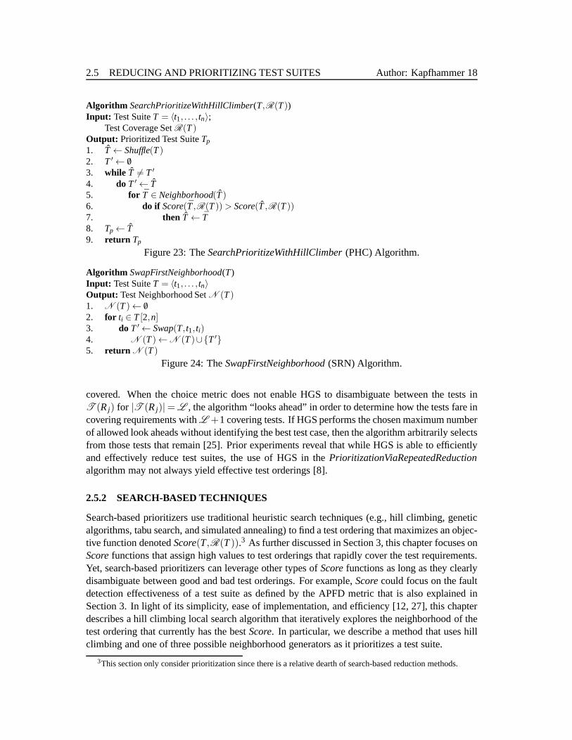
Search-based prioritizers use traditional heuristic search techniques (e.g., hill climbing, geneticalgorithms, tabu search, and simulated annealing) to find a test ordering that maximizes an objec-tive function denotedScore(T,R(T)).3 As further discussed in Section 3, this chapter focuses onScorefunctions that assign high values to test orderings that rapidly cover the test requirements.Yet, search-based prioritizers can leverage other types ofScorefunctions as long as they clearlydisambiguate between good and bad test orderings. For example, Scorecould focus on the faultdetection effectiveness of a test suite as defined by the APFDmetric that is also explained inSection 3. In light of its simplicity, ease of implementation, and efficiency [12, 27], this chapterdescribes a hill climbing local search algorithm that iteratively explores the neighborhood of thetest ordering that currently has the bestScore. In particular, we describe a method that uses hillclimbing and one of three possible neighborhood generatorsas it prioritizes a test suite.

3This section only consider prioritization since there is a relative dearth of search-based reduction methods.


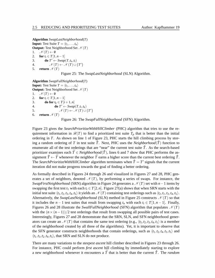
Algorithm SwapLastNeighborhood(T)Input: Test SuiteT = 〈t1, . . . , tn〉Output: Test Neighborhood SetN (T)1. N (T)← /02. for ti ∈ T[1,n−1]3. do T ′← Swap(T, tn, ti)4. N (T)←N (T)∪{T ′}5. return N (T)

Figure 25: TheSwapLastNeighborhood(SLN) Algorithm.

Algorithm SwapFullNeighborhood(T)Input: Test SuiteT = 〈t1, . . . , tn〉Output: Test Neighborhood SetN (T)1. N (T)← /02. for ti ∈ T[1,n−1]3. do for tk ∈ T[i +1,n]4. do T ′← Swap(T, ti , tk)5. N (T)←N (T)∪{T ′}6. return N (T)

Figure 26: TheSwapFullNeighborhood(SFN) Algorithm.

Figure 23 gives theSearchPrioritizeWithHillClimber(PHC) algorithm that tries to use the re-quirement information inR(T) to find a prioritized test suiteTp that is better than the initialordering inT. As shown on line 1 of Figure 23, PHC starts the hill climbing process by stor-ing a random ordering ofT in test suiteT. Next, PHC uses theNeighborhood(T) function toenumerate all of the test orderings that are “near” the current test suiteT. As the search-basedprioritizer examines eachT ∈ Neighborhood(T), lines 6 and 7 show that PHC performs the as-signmentT← T whenever the neighborT earns a higher score than the current best orderingT.TheSearchPrioritizeWithHillClimberalgorithm terminates whenT = T ′ signals that the currentiteration did not make progress towards the goal of finding a better ordering.

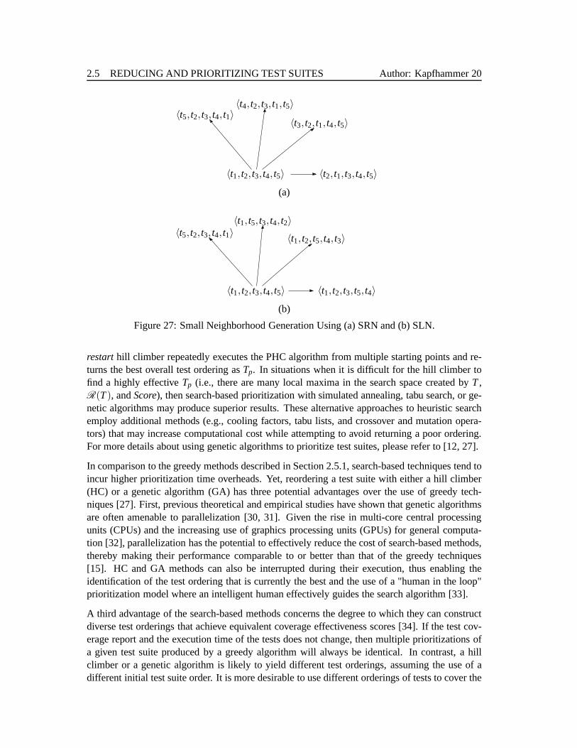
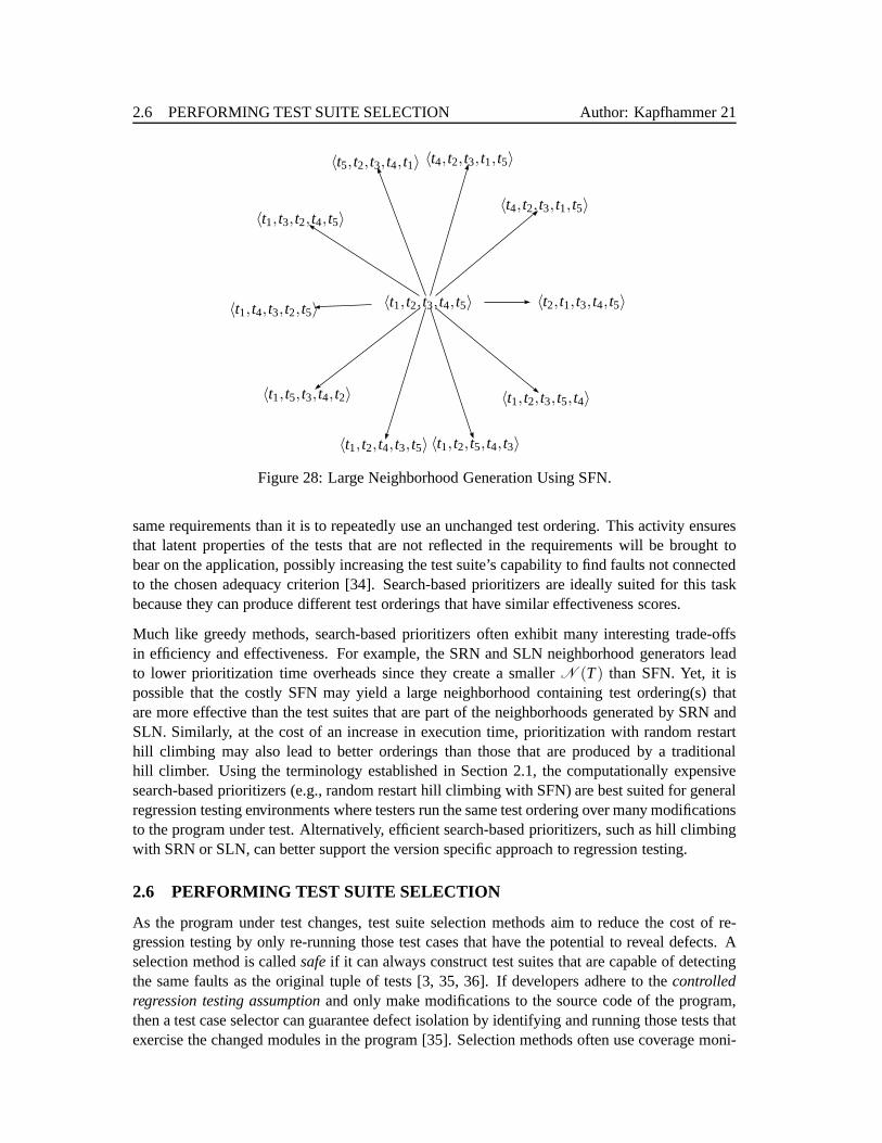
As formally described in Figures 24 through 26 and visualized in Figures 27 and 28, PHC gen-erates a set of neighbors, denotedN (T), by performing a series of swaps. For instance, theSwapFirstNeighborhood(SRN) algorithm in Figure 24 generates aN (T) set withn−1 items byswapping the first testt1 with eachti ∈ T[2,n]. Figure 27(a) shows that when SRN starts with theinitial test suite〈t1, t2, t3, t4, t5〉 it yields anN (T) containing test orderings such as〈t2, t1, t3, t4, t5〉.Alternatively, theSwapLastNeighborhood(SLN) method in Figure 25 constructsN (T) so thatit includes then− 1 test suites that result from swappingtn with eachti ∈ T[1,n− 1]. Finally,Figures 26 and 28 illustrate theSwallFullNeighborhood(SFN) algorithm that populatesN (T)with the(n× (n−1))/2 test orderings that result from swapping all possible pairs of test cases.Interestingly, Figures 27 and 28 demonstrate that the SRN, SLN, and SFN neighborhood gener-ators can create anN (T) that contains the same test ordering (e.g.,〈t5, t2, t3, t4, t1〉 is a memberof the neighborhood created by all three of the algorithms).Yet, it is important to observe thatthe SFN generator constructs neighborhoods that contain orderings, such as〈t1, t2, t4, t3, t5〉 and〈t1, t3, t2, t4, t5〉, that SRN and SLN do not produce.

There are many variations to thesteepest ascenthill climber described in Figures 23 through 26.For instance, PHC could performfirst ascenthill climbing by immediately starting to explorea new neighborhood whenever it encounters aT that is better than the currentT. The random


〈t1, t2, t3, t4, t5〉〈t2, t1, t3, t4, t5〉

〈t3, t2, t1, t4, t5〉

〈t4, t2, t3, t1, t5〉〈t5, t2, t3, t4, t1〉

(a)

〈t1, t2, t3, t4, t5〉〈t1, t2, t3, t5, t4〉

〈t1, t2, t5, t4, t3〉

〈t1, t5, t3, t4, t2〉〈t5, t2, t3, t4, t1〉

(b)

Figure 27: Small Neighborhood Generation Using (a) SRN and (b) SLN.

restarthill climber repeatedly executes the PHC algorithm from multiple starting points and re-turns the best overall test ordering asTp. In situations when it is difficult for the hill climber tofind a highly effectiveTp (i.e., there are many local maxima in the search space created by T,R(T), andScore), then search-based prioritization with simulated annealing, tabu search, or ge-netic algorithms may produce superior results. These alternative approaches to heuristic searchemploy additional methods (e.g., cooling factors, tabu lists, and crossover and mutation opera-tors) that may increase computational cost while attempting to avoid returning a poor ordering.For more details about using genetic algorithms to prioritize test suites, please refer to [12, 27].

In comparison to the greedy methods described in Section 2.5.1, search-based techniques tend toincur higher prioritization time overheads. Yet, reordering a test suite with either a hill climber(HC) or a genetic algorithm (GA) has three potential advantages over the use of greedy tech-niques [27]. First, previous theoretical and empirical studies have shown that genetic algorithmsare often amenable to parallelization [30, 31]. Given the rise in multi-core central processingunits (CPUs) and the increasing use of graphics processing units (GPUs) for general computa-tion [32], parallelization has the potential to effectively reduce the cost of search-based methods,thereby making their performance comparable to or better than that of the greedy techniques[15]. HC and GA methods can also be interrupted during their execution, thus enabling theidentification of the test ordering that is currently the best and the use of a "human in the loop"prioritization model where an intelligent human effectively guides the search algorithm [33].

A third advantage of the search-based methods concerns the degree to which they can constructdiverse test orderings that achieve equivalent coverage effectiveness scores [34]. If the test cov-erage report and the execution time of the tests does not change, then multiple prioritizations ofa given test suite produced by a greedy algorithm will alwaysbe identical. In contrast, a hillclimber or a genetic algorithm is likely to yield different test orderings, assuming the use of adifferent initial test suite order. It is more desirable to use different orderings of tests to cover the

2.6 PERFORMING TEST SUITE SELECTION Author: Kapfhammer 21

〈t1, t2, t3, t4, t5〉〈t2, t1, t3, t4, t5〉

〈t4, t2, t3, t1, t5〉

〈t4, t2, t3, t1, t5〉

〈t5, t2, t3, t4, t1〉

〈t1, t3, t2, t4, t5〉

〈t1, t4, t3, t2, t5〉

〈t1, t5, t3, t4, t2〉

〈t1, t2, t4, t3, t5〉〈t1, t2, t5, t4, t3〉

〈t1, t2, t3, t5, t4〉

Figure 28: Large Neighborhood Generation Using SFN.

same requirements than it is to repeatedly use an unchanged test ordering. This activity ensuresthat latent properties of the tests that are not reflected in the requirements will be brought tobear on the application, possibly increasing the test suite’s capability to find faults not connectedto the chosen adequacy criterion [34]. Search-based prioritizers are ideally suited for this taskbecause they can produce different test orderings that havesimilar effectiveness scores.

Much like greedy methods, search-based prioritizers oftenexhibit many interesting trade-offsin efficiency and effectiveness. For example, the SRN and SLNneighborhood generators leadto lower prioritization time overheads since they create a smaller N (T) than SFN. Yet, it ispossible that the costly SFN may yield a large neighborhood containing test ordering(s) thatare more effective than the test suites that are part of the neighborhoods generated by SRN andSLN. Similarly, at the cost of an increase in execution time,prioritization with random restarthill climbing may also lead to better orderings than those that are produced by a traditionalhill climber. Using the terminology established in Section2.1, the computationally expensivesearch-based prioritizers (e.g., random restart hill climbing with SFN) are best suited for generalregression testing environments where testers run the sametest ordering over many modificationsto the program under test. Alternatively, efficient search-based prioritizers, such as hill climbingwith SRN or SLN, can better support the version specific approach to regression testing.

2.6 PERFORMING TEST SUITE SELECTION

As the program under test changes, test suite selection methods aim to reduce the cost of re-gression testing by only re-running those test cases that have the potential to reveal defects. Aselection method is calledsafeif it can always construct test suites that are capable of detectingthe same faults as the original tuple of tests [3, 35, 36]. If developers adhere to thecontrolledregression testing assumptionand only make modifications to the source code of the program,then a test case selector can guarantee defect isolation by identifying and running those tests thatexercise the changed modules in the program [35]. Selectionmethods often use coverage moni-

2.6 PERFORMING TEST SUITE SELECTION Author: Kapfhammer 22

S1 S2

t1t2 t3t4t5 t6 t7

M1

t8t9

M3 M7

t10

M5

t11

M2 M4M8

t12

M9

t1→M3 means that testt1 exercisesmoduleM3

A box with roundedcorners denotes amodifiedmodule

A regular box indicates that a module hasnot changed

Figure 29: Test Suite Selection in the Presence of Changed Program Modules.

toring information to determine how the modules of the program are exercised by the tests. Afterrecording a coverage report and determining which modules were recently changed, the selectorexecutes a potentially smaller test suite that only focuseson these updated modules. Selectionmethods normally concentrate on program modifications involving the change, deletion, or ad-dition of a source code location. In practice, test suite selection techniques also need to track thechanges that the developers make to external resources (e.g., configuration files and databases).

Figure 29 depicts a test suite for a modified program containing a total of nine unique modulesthat may be Java methods or classes. As an example, this diagram uses the notationt1→M3 toindicate that the test caset1 exercisesmoduleM3. For each of the modules in Figure 29, a boxwith rounded corners highlights a module that recently underwent modification (e.g.,M3) whilea standard box means that developers did not change the module (e.g.,M9). Furthermore, thisexample usesS1 andS2 to respectively denote external resources that have and have not beenchanged by developers. A regression test selection mechanism analyzes coverage and changereports like the one in Figure 29 in order to determine which tests do not need to run becausethey did not exercise any modified modules (i.e.,t3, t4, t5, t7, andt12). After finding the teststhat (i) interact with methods using modified resources (e.g., t4, t8, t9, andt10) and (ii) directlyexercise the changed modules (i.e.,t1, t2, t6, t8, t9, andt11), a selection method can create and runa smaller test suite such as〈t1, t6, t8〉. In this instance, the selection mechanism must choose atest liket8 in order to ensure the testing of moduleM7’s interaction with the modified resourceS1. Furthermore, the technique picks tests such ast1 and t6 in order to ensure the isolation ofdefects that may arise from changes in modulesM1,M3, andM5.

Results from analytical studies, empirical evaluations, and practical experience suggest that thereare interesting trade-offs in the efficiency and effectiveness of test suite selection techniques. Forinstance, experiments conducted by Rothermel and Harrold indicate that test suite design canhave a substantial impact of the effectiveness of selectionmethods [36]. That is, selection maynot be cost-effective when the tests execute rapidly, the test suite is small, or there are certainmodules that are exercised by many test cases [36]. However,for situations like the one depictedin Figure 29, selection can often reduce testing time because each test focuses on a small number

2.7 RESOURCE-AWARE REGRESSION TESTING Author: Kapfhammer23

f1 f2 f3 f4 f5 f6 f7 f8t1 X X X X X X X

t2 X

t3 X X

t4 X X X

t5 X X X

t6 X X X

Faults Cost (Mins) Avg. Faults/Mint1 7 9 0.778t2 1 1 1.0t3 2 3 0.667t4 3 4 0.75t5 3 4 0.75t6 3 4 0.75

(a)

Time Limit: 12 minutesFault Time Avg. Faults/Min. Intelligent(Tp) (Tp) (Tp) (Tp)

t1 t2 t2 t5t3 t1 t4t4 t3t5

Total Faults 7 8 7 8Total Time 9 12 10 11

(b)

Figure 30: An Example of Time-Aware Test Suite Prioritization.

of modules (e.g.,t12 only interacts with four modules while many tests, such ast5 and t6, usejust one or two). Furthermore, the use of the Testar test selection tool at Google reveals that“the smaller your changes are (or the more frequently you runTestar), and the more tests youhave, the bigger are the relative savings” [37]. While conceding that test suite selection maynot be capable of decreasing testing time for some applications, Graves et al. observe that a safeselection method found all of the faults for which fault-identifying tests existed and discarded60% of the tests on the median [3]. Finally, selection methods may still identify small and usefultest suites in circumstances when the controlled regression testing assumption does not hold.

2.7 RESOURCE-AWARE REGRESSION TESTING

Several new regression testing methods aim to handle the challenges associated with runningtests in constrained environments where computational resources such as time, memory, or powerare limited [15]. This chapter considers the concrete example of time-aware test suite prioritiza-tion since time is a concern for organizations that rely uponnightly builds or perform regressiontesting each time source code changes are committed to a version control repository. As an ex-ample of time constrained testing, suppose that a tester wants to reorderT = 〈t1, t2, t3, t4, t5, t6〉,as shown in Figure 30. For the purposes of illustration, thisexample assumes a priori knowledgeof the faults detected byT in the programP. As given in Figure 30(a), test caset1 can find sevenfaults, { f1, f2, f4, f5, f6, f7, f8}, in nine minutes,t2 finds one fault,{ f1}, in one minute, andt3isolates two faults,{ f1, f5}, in three minutes. Test casest4, t5, andt6 each find three faults in fourminutes:{ f2, f3, f7}, { f4, f6, f8}, and{ f2, f4, f6}, respectively.

2.7 RESOURCE-AWARE REGRESSION TESTING Author: Kapfhammer24

Suppose that the time budget for regression testing is twelve minutes. Because we want to find asmany faults as possible early on, we order the test cases by only considering the number of faultsthat they can detect. Without a time budget, the test suiteT = 〈t1, t4, t5, t6, t3, t2〉 would execute.Out of this, only the test suiteTp = 〈t1〉 can run under a twelve minute time constraint, and itwould find a total of seven faults, as noted in Figure 30(b). Since time is a principal concern,it may also seem logical to order the test cases with regard totheir execution time. In the timeconstrained environment, a time-based prioritizationTp = 〈t2, t3, t4, t5〉 could be executed and findeight defects, as shown in Figure 30(b). Another option would be to consider the time budgetand fault information together. To do this, we could order the test cases according to the averagepercent of faults that they can detect per minute. Under the time constraint, the execution of theorderingTp = 〈t2, t1〉 finds a total of seven faults.

If the time budget and the fault information are both considered intelligently, that is, in a waythat accounts for overlapping fault detection, the test cases could be better prioritized and thusincrease the overall number of faults found in the desired time period. In this example, the testcases are intelligently reordered so that the suiteTp = 〈t5, t4, t3〉 is executed, revealing eight errorsin less time thanTp. It is also clear thatTp can reveal more defects thanTp andTp in the specifiedtesting time. Finally, it is important to note that the first two test cases ofTp, t2 and t3, find atotal of two faults in four minutes whereas the first test casein Tp, t5, detects three defects inthe same time period. The time-aware prioritization,Tp, is favored overTp because it is able todetect more faults earlier in test execution.

There are several different approaches to implementing a time-aware test prioritizer [15, 38,39]. For example, Walcott et al. present a genetic algorithmbased method that reorganizes testsuites so that the new order will (i) always run within a time limit and (ii) have the highestpossible potential for defect detection based upon the information in the coverage report [15].Alternatively, Alspaugh et al. describe an approach to efficient time-aware prioritization thatuses uses solvers for the 0/1 knapsack problem to reorder thetest suite [38]. In comparison to thegenetic algorithm, the knapsack solvers do not consider theoverlap in test coverage, thus quicklyproducing a test suite that is often less effective than the one constructed by the GA. Zhang et al.introduce a time-aware prioritizer that uses an integer linear programming (ILP) method to solvethe time and coverage constraints introducing by a restrictive testing time budget [39].

Recent experimental results indicate that higher levels ofcoverage and fault detection are ob-tained when time-aware prioritizers explicitly consider time constraints [15, 39]. Even when asevere time restriction forces testers to reduce the time allotted to testing by 75%, Walcott etal. report that their search-based technique preserves on average 94% of the original test suite’scode coverage [15]. Zhang et al. also find that certain traditional regression testing methods,such as those described in Section 2.5, may create reasonably effective test orderings when thetesting time budget is not too constrained. In these situations, it may make sense to use the tra-ditional greedy prioritizers since the non-time-aware techniques are normally cheaper than thosethat explicitly consider the testing time constraints. Finally, the experiments of Zhang et al. re-veal that the ILP-based solvers are often the most efficient and effective approach to time-awareprioritization, suggesting that this method may also be useful in quickly handling other resourceconstraints such as those related to memory and battery consumption [39].

EVALUATION OF REGRESSION TESTING TECHNIQUES Author: Kapfhammer 25

3 EVALUATION OF REGRESSION TESTING TECHNIQUES

During the use of regression testing in either an industrialenvironment or an experimental study,it is important to gauge the efficiency and effectiveness of the techniques that are described inSection 2. Since it is always desirable for a testing technique to run with low time and spaceoverheads, this section focuses on methods for measuring the effectiveness of approaches toselection, reduction, and prioritization. Equation (2) defines RFFS(T,Tr) ∈ [0,1), thereductionfactor for sizegiven a test suiteT and it’s reduced formTr [7]. Since the RFFS reflects the percentof original tests that remain after selection or reduction,an RFFS of 0 means that the algorithmremoved none of the tests while an RFFS near 1 means that the reducer discarded many tests (anRFFS of 1 is not possible because testers often mandate thatTr must contain at least one test tocover at least some of the requirements). As stated by Equations (3) and (4), RFFT(T,Tr)∈ [0,1)is thereduction factor for timefor test suitesT andTr [9]. An RFFT of 0 signifies thatT andTr execute for the same length of time (i.e.,time(T)− time(Tr) = 0) while an RFFT of 1 is theimpossible case whenTr executes instantaneously (i.e.,time(T)− time(Tr) = time(T)).

RFFS(T,Tr) =|T|− |Tr |

|T|(2) RFFT(T,Tr) =

time(T)− time(Tr)

time(T)(3)

time(T) = ∑ti∈T

time(ti) (4)

The majority of prior empirical research calculates the decrease in fault detection effectivenessfor a reduced test suite after seeding faults into the program under test (e.g., [7]). Yet, it is alsoimportant to use effectiveness metrics that do not require fault information since fault seedingmay be time consuming and error-prone. To this end, Equation(5) defines thereduction factorfor test requirementsas RFFR(T,Tr) ∈ [0,1]. Unlike the RFFS and RFFT metrics, we preferlow values for RFFR(T,Tr) because this indicates that a reduced test suiteTr covers the majorityof the requirements that the initial tests cover. To avoid confusion during the comparison ofdifferent reduction techniques, Equation (6) defines thepreservation factor for test requirements.If a reduced test suite has a high value for PFFR(T,Tr) ∈ [0,1], then we also know that it coversmost of the requirements that the original tests cover. Since the overlap-aware and custom greedyreduction algorithms defined in Section 2, such as GRO, HGS, and DGR, always create aTr thatcovers all of the test requirements we know that PFFR(T,Tr) = 1 for these methods. The otherreduction techniques (e.g., GR, RVR, and RAR) may not construct a test suite that covers allRj ∈R(T) and thus these methods may yield test suites with PFFR valuesthat are less than one.

RFFR(T,Tr) =|R(T)|− |R(Tr)|

|R(T)|(5)

PFFR(T,Tr) = 1−RFFR(T,Tr) (6)

In order to facilitate the comparison between different approaches to reduction, we use the tu-ple Er = 〈RFFS,RFFT,PFFR〉 to organize the evaluation metrics for test suiteTr .4 Figure 31

4Without loss of generality, this chapter concentrates on using RFFS, RFFT, and PFFR during the comparison ofreduction techniques. However, it is possible to apply the same approach ifE contains scores from different metrics.


Er Er Comparison

〈.4, .5, .8〉〈.4, .5, .9〉 Er ≫ Er

〈.4, .5,1〉〈.4, .55,1〉 Er ≫ Er

〈.6, .5,1〉〈.4, .5,1〉 Er ≫ Er

〈.4, .5,1〉〈.55, .75, .9〉 Er ∼ Er

Figure 31: Evaluation Tuples Used to Compare Reduced Test Suites.

summarizes the four different examples of evaluation tuples that this chapter uses to explainthe process of comparing different reduction algorithms. Suppose that two reduction techniquescreateTr andTr that are respectively characterized by the evaluation tuplesEr = 〈.4, .5, .8〉 andEr = 〈.4, .5, .9〉, found in the first row of the table in Figure 31. As a further aid in comparing re-duction methods, we use the notatione∈ Er ande∈ Er to clarify the tuple membership of scorese ande (i.e., RFFS refers to the reduction factor for size score inEr). In this example, a testerwould preferEr because it (i) has the same values for RFFS and RFFT (i.e., thereduction factorsfor the number of tests and the overall testing time) and (ii)preserves the coverage of more testrequirements sincePFFR> PFFR. IfEr = 〈.4, .5,1〉 andEr = 〈.4, .55,1〉, then we would favorthe reduced suite withEr because it fully preserves requirement coverage while yielding a largervalue for RFFS (i.e.,.55> .5). Next, suppose thatEr = 〈.6, .5,1〉 and Er = 〈.4, .5,1〉. In thissituation, we would favorEr ’s reduction algorithm since it yields the smallest test suite (i.e.,RFFS> RFFS). This choice is sensible because it will control testing time if there is an increasein the costs of starting up and shutting down an individual test case.

During the evaluation of reduction algorithms, it may not always be clear which technique is themost appropriate for a given program and its test suite. For example, assume thatEr = 〈.4, .5,1〉and Er = 〈.55, .75, .9〉, as provided by Figure 31. In this case,Er shows thatTr is (i) betterat reducing testing time and (ii) worse at preserving requirement coverage when we compareit to Tr . In this circumstance, a tester must choose the reduction technique that best fits thecurrent regression testing process. For instance, it may beprudent to selectEr when the testsuite is executed in a time and/or memory constrained environment (e.g., [15, 40]) or the testsare repeatedly run during continuous testing (e.g., [41]).If the correctness of the application isthe highest priority, then it is advisable to use the reduction technique that leads toTr andEr .

For the reduced test suitesTr andTr and their respective evaluation tuplesEr andEr , we writeEr ≫ Er when the logical predicate in Equation (7) holds (i.e., weprefer Tr to Tr). If Er ≫ Er ,then we know thatTr is as good asTr for all three evaluation metrics and better thanTr for atleast one metric.5 For instance, the first row of Figure 31 shows thatEr ≫ Er becauseTr yields(i) RFFS and RFFT values that are equal to the scores forTr and (ii) a PFFR value that is greaterthan that ofTr . If Equation (7) does not hold for test suitesTr andTr that were produced by twodifferent reduction techniques (i.e.,Er 6≫ Er andEr 6≫ Er), then we writeEr ∼ Er (i.e.,Tr andTr

aresimilar). Since Equation (7) does not dictate a preference betweenTr andTr whenEr ∼ Er ,as shown in the final row of Figure 31, a tester must use the constraints inherent in the testing

5Equation (7)’s definition of the≫ operator is based on the concept ofpareto efficiencythat is employed in thefields of economics and multi-objective optimization (please refer to [42] for more details about these areas).


Testing Time

. . .C

over

ed T

est R

eqs

t1 Done tn−1 Done

tn Done

CoverR(t1) Cover⋃n−1

i=1 R(ti)

CoverR(T)

Area=∫ time(T)

0C(T, l)

C(T

,l)

(l)

Figure 32: The Coverage Effectiveness of a Test Suite.

process to inform the choice of the best reduction technique. For instance, a tester may pick thefastest reducer whenEr ∼ Er and the developers wants to perform version specific testing.

∀e∈ Er , e∈ Er : (e≥ e) ∧ ∃ e∈ Er , e∈ Er : (e> e) (7)

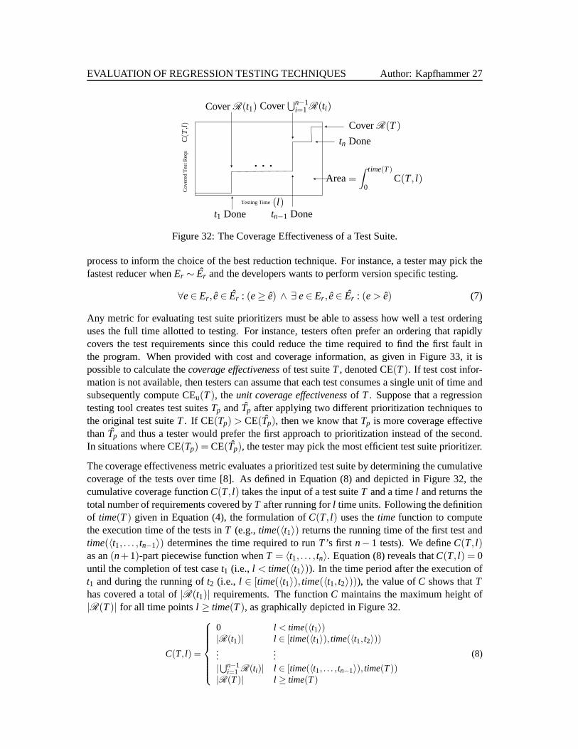
Any metric for evaluating test suite prioritizers must be able to assess how well a test orderinguses the full time allotted to testing. For instance, testers often prefer an ordering that rapidlycovers the test requirements since this could reduce the time required to find the first fault inthe program. When provided with cost and coverage information, as given in Figure 33, it ispossible to calculate thecoverage effectivenessof test suiteT, denoted CE(T). If test cost infor-mation is not available, then testers can assume that each test consumes a single unit of time andsubsequently compute CEu(T), theunit coverage effectivenessof T. Suppose that a regressiontesting tool creates test suitesTp andTp after applying two different prioritization techniques tothe original test suiteT. If CE(Tp) > CE(Tp), then we know thatTp is more coverage effectivethanTp and thus a tester would prefer the first approach to prioritization instead of the second.In situations where CE(Tp) = CE(Tp), the tester may pick the most efficient test suite prioritizer.

The coverage effectiveness metric evaluates a prioritizedtest suite by determining the cumulativecoverage of the tests over time [8]. As defined in Equation (8)and depicted in Figure 32, thecumulative coverage functionC(T, l) takes the input of a test suiteT and a timel and returns thetotal number of requirements covered byT after running forl time units. Following the definitionof time(T) given in Equation (4), the formulation ofC(T, l) uses thetime function to computethe execution time of the tests inT (e.g.,time(〈t1〉) returns the running time of the first test andtime(〈t1, . . . , tn−1〉) determines the time required to runT ’s first n− 1 tests). We defineC(T, l)as an(n+1)-part piecewise function whenT = 〈t1, . . . , tn〉. Equation (8) reveals thatC(T, l) = 0until the completion of test caset1 (i.e., l < time(〈t1〉)). In the time period after the execution oft1 and during the running oft2 (i.e., l ∈ [time(〈t1〉), time(〈t1, t2〉))), the value ofC shows thatThas covered a total of|R(t1)| requirements. The functionC maintains the maximum height of|R(T)| for all time pointsl ≥ time(T), as graphically depicted in Figure 32.

C(T, l) =

0 l < time(〈t1〉)|R(t1)| l ∈ [time(〈t1〉), time(〈t1, t2〉))...

...|⋃n−1

i=1 R(ti)| l ∈ [time(〈t1, . . . , tn−1〉), time(T))|R(T)| l ≥ time(T)

(8)


To formulate CE(T) ∈ (0,1), the integral ofC(T, l) is divided by the integral of the ideal cu-mulative coverage functionC(T, l) that Equation (9) defines to immediately cover all of therequirements. Equation (10) shows that CE considers test requirement coverage throughout theexecution time ofT by taking the integrals within the closed interval from 0 totime(T). Sinceany prioritization of a test suite should always cover the same requirements as the original order-ing (i.e.,R(T) =R(Tp)), our statement of coverage effectiveness forbids the caseof R(Tp) = /0that would lead to CE(T) = 0. Since it is impossible forTp to instantaneously cover all of the testrequirements, Equation (10)’s expression of coverage effectiveness also precludes CE(T) = 1.Finally, CEu(T) is defined in a similar manner to Equations (8) through (10), except for the factthat we assume all tests have unit cost and thustime(ti) = 1 for all ti ∈ T.

C(T, l) = |R(T)| (9) CE(T) =

∫ time(T)

0C(T, l)

∫ time(T)

0C(T, l)

(10)

Since many test coverage monitoring tools do not record the point in time when a test case cov-ers a requirement [20, 21], CE conservatively credits a testwith the coverage of its requirementswhen it finishes execution. While CE does furnish a time sensitive measurement of effective-ness, it may be unfair to high coverage tests with extended running times. One approach tohandling this issue is tolinearly interpolatebetween the points in the piece-wise coverage func-tion. For instance, the linear interpolant between the timewhen testing begins and the first testcase finishes execution is the straight line between the points (0,0) and(time(〈t1〉), |R(t1)|). Be-tween the time when an arbitraryt j ends and the following testt j+1 completes, Equation (11)definesCδ (T, l), the coverage function that performs linear interpolationbetween all of the points(time(〈t1, . . . , t j〉), | ∪

ji=1 R(ti)|) and(time(〈t1, . . . , t j+1〉), | ∪

j+1i=1 R(ti)|). TheC(T, l) function is

similar toCδ (T, l), except for the fact thatC exhibits abrupt “jumps” in height at the completionof each test case whereasCδ uses a straight line to approximate the increase in coverageas atest runs. Finally, Equation (12) calculates CEδ (T) in an analogous fashion to the one used forCE(T), with the exception of the fact that the numerator usesCδ instead ofC.

Cδ (T, l) =

l ×

(

|R(t1)|time(〈ti〉)

)

l < time(〈t1〉)

|R(t1)|+

(l − time(t1))+

(

|R(t1)∪R(t2)|−|R(t1)|time(〈t1,t2〉)−time(〈t1〉)

)

l ∈ [time(〈t1〉), time(〈t1, t2〉))

......

|⋃n−1

i=1 R(ti)|+

(l − time(〈t1, . . . , tn−1〉))×

(

|R(T)|−|⋃n−1

i=1 R(ti)|time(T)−time(〈t1,...,tn−1〉)

)

l ∈ [time(〈t1, . . . , tn−1〉), time(T))

|R(T)| l ≥ time(T)(11)

CEδ (T) =

∫ time(T)

0Cδ (T, l)

∫ time(T)

0C(T, l)

(12)


Test Case Cost (seconds) RequirementsR1 R2 R3 R4 R5

t1 5 X X

t2 10 X X X X

t3 4 X X X

Total Testing Time = 19 seconds

Figure 33: The Cost and Coverage Characteristics of a Test Suite.

As an example of calculating coverage effectiveness, suppose that test suiteT = 〈t1, t2, t3〉 cov-ers a total of five requirements while testing programP. Figure 33 characterizes test suiteTaccording to execution time and requirement coverage (e.g., testt2 takes ten seconds to executewhile t1 andt3 respectively consume five and four seconds). Figure 34 visualizes the coveragecurves and gives the CE and CEu values for the 3!= 3× 2×1 = 6 different orderings of testsuiteT. These graphs demonstrate that the inclusion of test case execution costs does impact themeasurement of effectiveness. For instance, CEu equivalently ranks the orderingsTp = 〈t1, t2, t3〉andTp = 〈t1, t3, t2〉 while CE classifies the latter as more effective. This resultis due to the factthat Tp’s first two tests cover four requirements in nine seconds while the corresponding tests inTp take fifteen seconds to cover four requirements.

For a given test order, CE may be higher than CEu or vice-versa. For instance,〈t2, t1, t3〉 results ina low value for CE and a high CEu score because CE incorporates the substantial cost of runningt2 and CEu assumes thatt2’s running time is equivalent to the other tests. Figure 35 furnishesthe graphs for the linearly interpolating coverage function Cδ and the corresponding CEδ values.A comparison of Figure 34(a) and Figure 35 reveals that CEδ ’s use of interpolation uniformlyincreases the coverage effectiveness score. Finally, these eighteen graphs illustrate that differenttest orderings are more or less effective at using the amountof time devoted to testing.

In contrast to CE, other evaluation metrics such as theaverage percentage of faults detected(APFD) [5] do not factor time into the evaluation of a test suite prioritizer. Unlike existingevaluation metrics that incorporate time (e.g., APFDc [43]), CE obviates the need to use fault in-formation when calculating effectiveness. However, if per-test fault information, like that in Fig-ure 36, is available from testing records or seeded faults, then testers may pursue the calculationof APFD. For a set of known faultsF, Equation (13) defines the APFD(T,F) ∈ [ 1

2×|T| ,1−1

2×|T| ]

when reveal( f ,T) denotes the position withinT of the first test that reveals faultf ∈ F [44].Using this formulation of APFD, the minimum value of12×|T| corresponds to the circumstance inwhich the last test case in the ordering is the first to expose all of the faults. Moreover, the maxi-mum value of 1− 1

2×|T| is evident when the first test can find all of the faults. If we use the test

orderingsTp = 〈t1, t2, t3, t4, t5〉 andTp = 〈t3, t4, t1, t2, t5〉 and the fault information in Figure 36 asan example, then we have APFD(Tp,F) = 1− .4+ .1= .7 and APFD(Tp,F) = 1− .2+ .1= .82.This result suggests that, according to the APFD metric,Tp is a better prioritization thanTp.

APFD(T,F) = 1−∑ f∈F reveal( f ,T)

|T|× |F|+

12×|T|

(13)


0 5 10 15

01

23

45

Testing Time (l)Cov

ered

Tes

t Req

uire

men

ts (

C(T

, l))

1, 2, 3 CE = 0.3789

0 5 10 15

01

23

45

Testing Time (l)Cov

ered

Tes

t Req

uire

men

ts (

C(T

, l))

1, 3, 2 CE = 0.5053

0 5 10 15

01

23

45

Testing Time (l)Cov

ered

Tes

t Req

uire

men

ts (

C(T

, l))

2, 1, 3 CE = 0.3789

0 5 10 15

01

23

45

Testing Time (l)Cov

ered

Tes

t Req

uire

men

ts (

C(T

, l))

2, 3, 1 CE = 0.4316

0 5 10 15

01

23

45

Testing Time (l)Cov

ered

Tes

t Req

uire

men

ts (

C(T

, l))

3, 1, 2 CE = 0.5789

0 5 10 15

01

23

45

Testing Time (l)Cov

ered

Tes

t Req

uire

men

ts (

C(T

, l))

3, 2, 1 CE = 0.5789

(a)

0.0 1.0 2.0 3.0

01

23

45

Testing Time (l)Cov

ered

Tes

t Req

uire

men

ts (

C(T

, l))

1, 2, 3 CE = 0.4

0.0 1.0 2.0 3.0

01

23

45

Testing Time (l)Cov

ered

Tes

t Req

uire

men

ts (

C(T

, l))

1, 3, 2 CE = 0.4

0.0 1.0 2.0 3.0

01

23

45

Testing Time (l)Cov

ered

Tes

t Req

uire

men

ts (

C(T

, l))

2, 1, 3 CE = 0.5333

0.0 1.0 2.0 3.0

01

23

45

Testing Time (l)Cov

ered

Tes

t Req

uire

men

ts (

C(T

, l))

2, 3, 1 CE = 0.6

0.0 1.0 2.0 3.0

01

23

45

Testing Time (l)Cov

ered

Tes

t Req

uire

men

ts (

C(T

, l))

3, 1, 2 CE = 0.4667

0.0 1.0 2.0 3.0

01

23

45

Testing Time (l)Cov

ered

Tes

t Req

uire

men

ts (

C(T

, l))

3, 2, 1 CE = 0.5333

(b)

Figure 34: The (a) CE(T) and (b) CEu(T) Scores forT = 〈t1, t2, t3〉.


0 5 10 15

01

23

45

Testing Time (l)Cov

ered

Tes

t Req

uire

men

ts (

Cδ(T

, l))

1, 2, 3 CEδ = 0.5579

0 5 10 15

01

23

45

Testing Time (l)Cov

ered

Tes

t Req

uire

men

ts (

Cδ(T

, l))

1, 3, 2 CEδ = 0.6526

0 5 10 15

01

23

45

Testing Time (l)Cov

ered

Tes

t Req

uire

men

ts (

Cδ(T

, l))

2, 1, 3 CEδ = 0.6105

0 5 10 15

01

23

45

Testing Time (l)Cov

ered

Tes

t Req

uire

men

ts (

Cδ(T

, l))

2, 3, 1 CEδ = 0.6632

0 5 10 15

01

23

45

Testing Time (l)Cov

ered

Tes

t Req

uire

men

ts (

Cδ(T

, l))

3, 1, 2 CEδ = 0.721

0 5 10 15

01

23

45

Testing Time (l)Cov

ered

Tes

t Req

uire

men

ts (

Cδ(T

, l))

3, 2, 1 CEδ = 0.7474

Figure 35: The CEδ (T) Scores forT = 〈t1, t2, t3〉.

Several recent empirical studies have shown that certain types of test suites are relatively easyto prioritize [8, 9, 11]. If a regression test suiteT contains many tests that cover a substantialnumber of the requirements, then a random reordering ofT may often have a CE value that isgreater than the CE score for the initial ordering [8, 9]. Similarly, a random prioritization mayimprove the APFD of a test suite containing many tests that detect a large number of faults [11].Equation (14) defines D(T,R) ∈ (0,1], thecoverage densityof test suiteT for requirement setR. A low value for D(T,R) suggests that many test cases cover a small number of requirements,while D(T,R) = 1 indicates that each test case covers all of the requirements. If we assume thateach of the requirements inR(T) must be covered by one of the tests withinT, then every testsuite will have a density value greater than zero. A random prioritizer may be sufficient for testsuites that have a high value for D, whereas a low D value indicates the need for the greedy andsearch-based approaches. For example, the test suite in Figure 10 yields the relatively low valueof D(T,R) = .2619. Finally, Figure 37 furnishes an empirical cumulativedistribution function(ECDF) that visualizes the range of|R(ti)| values for the test suite in Figure 10. An ECDF givesthe cumulative percentage of the data set whose values fall below a specific value [45]. As aconfirmation of the test suite’s low density value, this ECDFreveals that 80% of the test cases inFigure 10 have anR(ti) set containing two or fewer requirements.

D(T,R) =∑ti∈T |R(ti)|

|T|× |F|(14)

CONCLUSIONS AND FUTURE WORK Author: Kapfhammer 32

Test Case Faultsf1 f2 f3 f4 f5

t1 X X

t2 X X

t3 X X X

t4 X X X

t5 X X

Figure 36: The Faults Detected by a Test Suite.

4 CONCLUSIONS AND FUTURE WORK

This chapter examines an important software maintenance activity known as regression testing.Methods for regression testing focus on running a test suitewhenever the addition of defect fixesor new functionality causes the program under test to change. Even though the use of regres-sion testing techniques often leads to software applications with high observed quality [2], therepeated execution of test cases can be so costly that it accounts for half the cost of maintaining asoftware system [3]. This chapter focuses on reduction methods that decrease the cost of testingby discarding those tests that redundantly cover the test requirements. Additionally, the chapterdescribes approaches to test suite prioritization that reorder a test suite in an attempt to improvethe rate at which tests achieve certain testing goals such asrequirement coverage. Finally, wereport on test selection techniques that reduce the cost of testing by only running those tests thatexercise the recently modified modules of the program. Thesemethods for enhancing regressiontest suites have different trade-offs in efficiency and effectiveness, thus making them more orless useful in the general and version specific models of regression testing.

After furnishing a detailed description of greedy and search-based techniques for prioritizationand reduction, this chapter highlights safe test selectionmethods. We also note that the reduc-tion factors for size and time and the preservation factor for test requirements are three metricsthat facilitate the comparison between different approaches to reduction. As long as a methodincurs minimal time and space overheads while preserving requirement coverage, a tester wouldnormally pick a test reducer that substantially decreases the size and running time of a test suite.In the context of test suite prioritization, evaluation metrics such as coverage effectiveness andthe average percentage of faults detected must determine how well a regression test suite usesthe given time to cover requirements or detect faults.

In light of the wide range of advances in this field, technology transfer represents an importantstep for further work in regression testing. To date, many important methods for running andanalyzing test suites have not transitioned into practice due to the lack of properly documentedand supported tools. The existence of freely available and open source testing tools that integratewith existing frameworks such as JUnit and CppUnit will be beneficial to both testing researchersand practitioners. However, as noted by Frederick P. BrooksJr., the greatest hope that the soft-ware engineering community has for solving the crisis of lowquality software is exceptionalengineers and testers [46]. As such, the proper education and training of testing students andprofessionals is an important area for further investigation. In summary, future progress in re-gression testing research, the development of new testing tools, and the education of testers allstand to substantially benefit a modern society that is increasingly reliant upon software.

FURTHER INFORMATION Author: Kapfhammer 33

0 1 2 3 4

0.0

0.2

0.4

0.6

0.8

1.0

Size of the Covered Requirement Sets − |R(ti)|

Em

piric

al C

DF

Figure 37: An ECDF of the Covered Requirement Sets for the Test Suite in Figure 10.

5 FURTHER INFORMATION

The ACM/IEEE International Conference on Software Engineering, the ACM SIGSOFT Sympo-sium on the Foundations of Software Engineering, the ACM SIGSOFT International Symposiumon Software Testing and Analysis, and the ACM SIGAPP Symposium on Applied Computing’sSoftware Engineering Track are all important forums for newresearch in the area of regressiontesting. Other important conferences include: IEEE/ACM Automated Software Engineering,IEEE International Conference on Software Maintenance, IEEE International Symposium onSoftware Reliability Engineering, IEEE/ACM International Symposium on Empirical SoftwareEngineering and Measurement, IEEE/NASA Software Engineering Workshop, and IEEE Com-puter Software and Applications Conference. TheIEEE Transactions on Software Engineeringand theACM Transactions on Software Engineering and Methodologyare two noteworthy jour-nals that publish regression testing papers. Other journals include:Software Testing, Verification,and Reliability, Software: Practice and Experience, Software Quality Journal, Automated Soft-ware Engineering: An International Journal, Empirical Software Engineering: An InternationalJournal, andInformation and Software Technology. Magazines that publish software testing arti-cles includeCommunications of the ACM, IEEE Software, IEEE Computer, andBetter Software(formerly known asSoftware Testing and Quality Engineering). ACM SIGSOFT also sponsorsthe bi-monthly newsletter calledSoftware Engineering Notes.

Acknowledgments. The biblical verse “Test everything. Hold on to the good” from Thessalo-nians 5:21 (New International Version) has served as a constant source of motivation during thecompletion of this chapter. The constructive feedback and valuable assistance from Adam Smith,Alexander Conrad, Zachary Williams, and Arpan Agrawal havebetter enabled me to produce achapter that will hopefully “pass the test” and ultimately be “held on to” by readers.

References

[1] Akira K. Onoma, Wei-Tek Tsai, Mustafa Poonawala, and Hiroshi Suganuma. Regression testing inan industrial environment.Communications of the ACM, 41(5), 1998.

[2] Mechelle Gittens, Hanan Lutfiyya, Michael Bauer, David Godwin, Yong Woo Kim, and PramodGupta. An empirical evaluation of system and regression testing. In Proceedings of the Conference

REFERENCES Author: Kapfhammer 34

of the Centre for Advanced Studies on Collaborative Research, 2002.

[3] Todd L. Graves, Mary Jean Harrold, Jung-Min Kim, Adam Porter, and Gregg Rothermel. An empir-ical study of regression test selection techniques.ACM Transactions on Software Engineering andMethodology, 10(2), 2001.

[4] Gregory M. Kapfhammer.The Computer Science Handbook, chapter 105: Software Testing. CRCPress, Boca Raton, FL, second edition, 2004.

[5] Gregg Rothermel, Roland J. Untch, and Chengyun Chu. Prioritizing test cases for regression testing.IEEE Transactions on Software Engineering, 27(10), 2001.

[6] Dick Hamlet and Joe Maybee.The Engineering of Software. Addison Wesley, Boston, MA, 2001.

[7] Scott McMaster and Atif M. Memon. Call stack coverage fortest-suite reduction. InProceedingsof the 21st International Conference on Software Maintenance, 2005.

[8] Adam M. Smith and Gregory M. Kapfhammer. An empirical study of incorporating cost into testsuite reduction and prioritization. InProceedings of the 24th Symposium on Applied Computing,2009.

[9] Gregory M. Kapfhammer.A Comprehensive Framework for Testing Database-Centric Applications.PhD thesis, University of Pittsburgh, Pittsburgh, Pennsylvania, 2007.

[10] Hao Zhong, Lu Zhang, and Hong Mei. An experimental studyof four typical test suite reductiontechniques.Information and Software Technology, 50(6), 2008.

[11] Sreedevi Sampath, Renee C. Bryce, Gokulanand Viswanath, Vani Kandimalla, and A. Gunes Koru.Prioritizing user-session-based test cases for web applications testing. InProceedings of the 2ndInternational Conference on Software Testing, Verification, and Validation, 2008.

[12] Zheng Li, Mark Harman, and Robert M. Hierons. Search algorithms for regression test case priori-tization. IEEE Transactions on Software Engineering, 33(4), 2007.

[13] Sebastian Elbaum, Alexey G. Malishevsky, and Gregg Rothermel. Test case prioritization: A familyof empirical studies.IEEE Transactions on Software Engineering, 28(2), 2002.

[14] David S. Rosenblum and Elaine J. Weyuker. Using coverage information to predict the cost-effectiveness of regression testing strategies.IEEE Transactions on Software Engineering, 23(3),1997.

[15] Kristen R. Walcott, Mary Lou Soffa, Gregory M. Kapfhammer, and Robert S. Roos. Time-awaretest suite prioritization. InProceedings of the International Symposium on Software Testing andAnalysis, 2006.

[16] Christian Murphy, Kuang Shen, and Gail Kaiser. Automatic system testing of programs without testoracles. InProceedings of the International Symposium on Software Testing and Analysis, 2009.

[17] Jeffrey M. Voas. PIE: a dynamic failure-based technique. IEEE Transactions on Software Engineer-ing, 18(8):717–735, 1992.

[18] Monica Hutchins, Herb Foster, Tarak Goradia, and Thomas Ostrand. Experiments on the effective-ness of dataflow- and controlflow-based test adequacy criteria. In Proceedings of the 16th Interna-tional Conference on Software Engineering, 1994.


[19] Matthew Rummel, Gregory M. Kapfhammer, and Andrew Thall. Towards the priortiziation of re-gression test suites with data flow information. InProceedings of the 20th Symposium on AppliedComputing, 2005.

[20] Jonathan Misurda, James A. Clause, Juliya L. Reed, Bruce R. Childers, and Mary Lou Soffa.Demand-driven structural testing with dynamic instrumentation. In Proceedings of the 27th In-ternational Conference on Software Engineering, 2005.

[21] Gregory M. Kapfhammer and Mary Lou Soffa. Database-aware test coverage monitoring. InPro-ceedings of the 1st India Software Engineering Conference, 2008.

[22] Scott McMaster and Atif Memon. Call stack coverage for GUI test-suite reduction. InProceedingsof the 17th International Symposium on Software Reliability Engineering, 2006.

[23] Scott McMaster and Atif M. Memon. Fault detection probability analysis for coverage-based testsuite reduction. InProceedings of the 23rd International Conference on Software Maintenance,2007.

[24] Vijay V. Vazirani.Approximation algorithms. Springer-Verlag New York, Inc., New York, NY, USA,2001.

[25] Mary Jean Harrold, Rajiv Gupta, and Mary Lou Soffa. A methodology for controlling the size of atest suite.ACM Transactions on Software Engineering and Methodology, 2(3), 1993.

[26] Sriraman Tallam and Neelam Gupta. A concept analysis inspired greedy algorithm for test suiteminimization. InProceedings of the 6th Workshop on Program Analysis for Software Tools andEngineering, 2005.

[27] Alexander Conrad, Robert S. Roos, and Gregory M. Kapfhammer. Empirically studying the role ofselection operators during search-based test suite prioritization. InProceedings of the Genetic andEvolutionary Computation Conference, 2010.

[28] Hyunsook Do, Gregg Rothermel, and Alex Kinneer. Empirical studies of test case prioritizationin a JUnit testing environment. InProceedings of the 15th International Symposium on SoftwareReliability Engineering, 2004.

[29] Jon L. Bentley and M. Douglas McIlroy. Engineering a sort function. Software, Practice, andExperience, 23(11):1249–1265, 1993.

[30] Erick Cantu-Paz.Efficient and Accurate Parallel Genetic Algorithms. Kluwer Academic Publishers,2000.

[31] Brian Zorman, Gregory M. Kapfhammer, and Robert S. Roos. Creation and analysis of a JavaSpace-based genetic algorithm. InProceedings of the 8th International Conference on Parallel and Dis-tributed Processing Techniques and Applications, Las Vegas, NV, June 2002.

[32] Tong Li, Dan Baumberger, David A. Koufaty, and Scott Hahn. Efficient operating system schedulingfor performance-asymmetric multi-core architectures. InProceedings of the Conference on Super-computing, 2007.

[33] Shin Yoo, Mark Harman, Paolo Tonella, and Angelo Susi. Clustering test cases to achieve effectiveand scalable prioritisation incorporating expert knowledge. In Proceedings of the InternationalSymposium on Software Testing and Analysis, 2009.

[34] Shin Yoo, Mark Harman, and Shmuel Ur. Measuring and improving latency to avoid test suite wearout. InProceedings of the Workshop on Search-Based Software Testing, 2009.


[35] G. Rothermel and M. J. Harrold. A safe, efficient regression test selection technique.ACM Trans-actions on Software Engineering and Methodology, 6(2), April 1997.

[36] G. Rothermel and M. J. Harrold. Empirical studies of a safe regression test selection technique.IEEE Transactions on Software Engineering, 24(6):401–419, June 1998.

[37] Testar - selective testing tool for Java. 2009. http://google-testar.sourceforge.net/.

[38] Sara Alspaugh, Kristen R. Walcott, Michael Belanich, Gregory M. Kapfhammer, and Mary LouSoffa. Efficient time-aware prioritization with knapsack solvers. InProceedings of the Workshop onEmpirical Assessment of Software Engineering Languages and Technologies, 2007.

[39] Lu Zhang, Shan-Shan Hou, Chao Guo, Tao Xie, and Hong Mei.Time-aware test-case prioritizationusing integer linear programming. InProceedings of the International Symposium on SoftwareTesting and Analysis, 2009.

[40] Gregory M. Kapfhammer, Mary Lou Soffa, and Daniel Mosse. Testing in resource constrained ex-ecution environments. InProceedings of the 20th International Conference on Automated SoftwareEngineering, 2005.

[41] David Saff and Michael D. Ernst. An experimental evaluation of continuous testing during develop-ment. InProceedings of the International Symposium on Software Testing and Analysis, 2004.

[42] Eckart Zitzler and Lothar Thiele. Multi-objective evolutionary algorithms: a comparative case studyand the strength pareto approach.IEEE Transactions on Evolutionary Computation, 3(4), 1999.

[43] A. G. Malishevsky, J. Ruthruff, G. Rothermel, and S. Elbaum. Cost-cognizant test case prioritization.Technical Report TR-UNL-CSE-2006-0004, University of Nebraska - Lincoln, 2006.

[44] Sebastian Elbaum, Gregg Rothermel, Satya Kanduri, andAlexey G. Malishevsky. Selecting a cost-effective test case prioritization technique. Technical Report 03-01-01, Department of ComputerScience and Engineering, University of Nebraska – Lincoln,January 2003.

[45] Shirley Dowdy, Stanley Wearden, and Daniel Chilko.Statistics for Research. Wiley-Interscience,third edition, 2004.

[46] Jr. Frederick P. Brooks.The Mythical Man-Month. Addison-Wesley, Reading, Massachusetts, 1995.

regression testing - department of computer science - allegheny

Documents