regression models with ordinal...

REGRESSION MODELS WITH ORDINAL VARIABLES*

CHRISTOPHER WINSHIP

Northwestern University and Economics Research Center/NORC

ROBERT D. MARE

University of Wisconsin-Madison

Most discussions of ordinal variables in the sociological literature debate the suitability of linear regression and structural equation methods when some variables are ordinal. Largely ignored in these discussions are methods for ordinal variables that are natural extensions of probit and logit models for dichotomous variables. If ordinal variables are discrete realizations of unmeasured continuous variables, these methods allow one to include ordinal dependent and independent variables into structural equation models in a way that (I) explicitly recognizes their ordinality, (2) avoids arbitrary assumptions about their scale, and (3) allows for analysis of continuous, dichotomous, and ordinal variables within a common statistical framework. These models rely on assumed probability distributions of the continuous variables that underly the observed ordinal variables, but these assumptions are testable. The models can be estimated using a number of commonly used statistical programs. As is illustrated by an empirical example, ordered probit and logit models, like their dichotomous counterparts, take account of the ceiling andfloor restrictions on models that include ordinal variables, whereas the linear regression model does not.

Empirical social research has benefited dur- ing the past two decades from the application of structural equation models for statistical analysis and causal interpretation of multivariate relationships (e.g., Goldberger and Duncan, 1973; Bielby and Hauser, 1977). Structural equation methods have mainly been applied to problems in which variables are measured on a continuous scale, a reflection of the availability of the theories of multivariate analysis and general linear models for continuous variables. A recurring methodological issue has been how to treat variables measured on an ordinal scale when multiple regression and structural equation methods would otherwise be appropriate tools. Many articles have appeared in this journal (e.g., Bollen and Barb, 1981, 1983; Henry, 1982; Johnson and Creech, 1983; O'Brien, 1979a, 1983) and elsewhere (e.g., Blalock, 1974; Kim, 1975, 1978; Mayer and Robinson, 1978; O'Brien 1979b, 1981,

1982) that discuss whether, on the one hand, ordinal variables can be safely treated as if they were continuous variables and thus ordinary linear model techniques applied to them, or, on the other hand, ordinal variables require special statistical methods or should be replaced with truly continuous variables in causal models. Allan (1976), Borgatta (1968), Kim (1975, 1978), Labovitz (1967, 1970), and O'Brien (1979a), among others, claim that multivariate methods for interval-level variables should be used for ordinal variables because the power and flexibility gained from these methods out- weigh the small biases that they may entail. Hawkes (1971), Morris (1970), O'Brien (1982), Reynolds (1973), Somers (1974), and Smith (1974), among others, suggest that the biases in using continuous-variable methods for ordinal variables are large and that special techniques for ordinal variables are required.

Although the literature on ordinal variables in sociology is vast, its practical implications have been few. Most researchers apply regression, MIMIC, LISREL, and other multivariate models for continuous variables to ordinal variables, sometimes claiming support from studies that find little bias from assuming interval measurement for ordinal variables. Yet these studies as well as the ones that they crit- icize provide no solid guidance because they are typically atheoretical simulations of limited scope. Somp researchers apply recently devel- oped techniques for categorical-data analysis that take account of the ordering of the categories of variables in cross-classifications (e.g., Agresti, 1983; Clogg, 1982; Goodman,

*Direct all correspondence to: Robert D. Mare, Department of Sociology, University of Wisconsin, 1180 Observatory Dr., Madison, WI 53706.

The authors contributed equally to this article. This research was supported by the National Science Foundation. Mare was supported by the University of Wisconsin-Madison Graduate School, the Center for Advanced Study in the Behavioral Sciences (through the National Science Foundation), and the Wisconsin Center for Education Research. Winship was supported by NORC and a Faculty Research Grant from Northwestern University. The authors are grateful to Ian Domowitz and Henry Farber for helpful advice, and to Lynn Gale, Ann Kremers, and Ernie Woodward for research assistance.

512 American Sociological Review, 1984, Vol. 49 (August:512-525)

REGRESSION MODELS WITH ORDINAL VARIABLES 513

1980). These methods, however, while elegant and well grounded in statistical theory, are dif- ficult to use in the cases where regression analysis and its extensions would otherwise apply: that is, where data are nontabular; include continuous, discrete, and ordinal variables; and apply to a causal model with several endogenous variables.

This article draws attention to alternative methods for estimating regression models and their generalizations that include ordinal variables. These methods are extensions of logit and probit models for dichotomous variables and are based on models that include unmeasured continuous variables for which only ordinal measures are available. Largely ignored in the sociological literature (though see McKelvey and Zavoina, 1975), they provide multivariate models with ordinal variables that: (1) take account of noninterval ordinal measurement; (2) avoid arbitrary assumptions about the scale of ordinal variables; and, most importantly, (3) include ordinal variables in structural equation models with variables at all levels of measurement. The ordered probit and logit models can, moreover, be implemented with widely available statistical software. Most of the literature on these methods focuses on estimating equations with ordinal dependent variables (Aitchison and Silvey, 1957; Amemiya, 1975; Ashford, 1959; Cox, 1970; Gurland et al., 1960; Maddala, 1983; McCul- lagh, 1980; McKelvey and Zavoina 1975), though some of it is relevant to models with ordinal independent variables (Heckman, 1978; Winship and Mare, 1983). Taken together, these contributions imply that ordinal variables can be analyzed within structural equation models with the same flexibility and power that are available for continuous variables.

This article summarizes the probit and logit models for ordered variables. It describes measurement models for ordinal variables and discusses specification and estimation of models with ordinal dependent and independent variables. Then it discusses some tests for model misspecification. Finally, it presents an empirical example which illustrates the models. An appendix discusses several technical topics of interest to those who wish to implement the models.

MEASUREMENT OF ORDINAL VARIABLES

A common view of ordinal variables, which is adopted here, is that they are nonstrict monotonic transformations of interval variables (e.g., O'Brien, 1981). That is, one or more values of an interval-level variable are mapped into the same value of a transformed,

ordinal variable. For example, a Likert scale may place individuals in one of a number of ranked categories, such as, "strongly agree," "somewhat agree," "neither agree nor disagree," "somewhat disagree," or " strongly disagree" with a statement. An underlying, continuous variable denoting individuals' degrees of agreement is mapped into categories that are ordered but are separated by unknown distances. I

This view of ordinal variables can also apply to variables that are often treated as continuous but might be better viewed as ordinal. Counted variables, such as grades of school completed, number of children ever born, or number of voluntary-association memberships, may be regarded as ordinal realizations of underlying continuous variables. Grades of school, for example, should be viewed as an ordinal measure of an underlying variable, "educational attainment," when one wishes to acknowledge that each grade is not equally easy to attain (e.g., Mare, 1980) or equally rewarding (e.g., Featherman and Hauser, 1978; Jencks et al., 1979). Similarly, when a continuous variable, such as earnings, is measured in categories corresponding to dollar intervals and category midpoints are unknown, the measured variable is an ordinal representation of an underlying continuous variable.2

The measurement model of ordinal variables can be stated formally as follows. Let Y denote an unobserved, continuous variable (-w < Y < o) and a0, al, . . a, J-1, aj denote cut-points in the distribution of Y, where a0 = - x and aj = ? (see Figure 1). Let Y* be an ordinal variable such that

y= j if aj- , Y < aj (j= 1,..,J).

I A less common type of ordinal variable, not discussed further ini this article, may result from a strict monotonic transformation of an interval variable. That is, observations (e.g., of cities, persons, occu- pations, etc.) may be ranked according to some unmeasured criterion (e.g., population size, wealth, rate of pay, etc.). A regression model with a ranked dependent variable requires that the nonlinear mapping between the unmeasured continuous ranking variable and the ranks themselves be specified. Given the mapping, the model can be estimated by nonlinear least squares (e.g., Gallant, 1975).

2 The ordinal-variable model can be extended to take account of measurement error. That is, an ordinal variable is a transformation of a continuous variable, but some observations may be misclassified (O'Brien, 1981; Johnson and Creech, 1983). Al- though this article does not discuss this complica- tion, it is a logical extension of the models presented here. Muthen (1979), Avery and Hotz (1982), and Winship and Mare (1983) discuss this extension for dichotomous variables; Muthen (1983, 1984) discusses it for ordinal variables.

514 AMERICAN SOCIOLOGICAL REVIEW

f(Y)

/(Y - J) - F(= - )

1 j-1 j J-1

Figure 1. Relationships Among Latent Continuous Variable (Y), Observed Ordinal Variable (Y*), and Thresholds (aj)

Since Y is not observed, its mean and variance are unknown and their values must be assumed. For the present, assume that Y has mean of zero and variance of one.

The relationship between Y and Y* can be further understood as follows. Consider the likelihood of obtaining a particular value of Y and the probability that Y* takes on a specific value (see Figure 1). If Y follows a probability distribution (for example, normal) with density function f(Y) and cumulative density function F(Y), then the probability that Y* = j is the area under the density curve f(Y) between aj-1 and aj. That is,

ai P(Y* =j) = f f(Y)dy=F(aj)-F(aj_), (1)

where F(aj) = 1 and F(a0) = 0. For a sample of individuals for whom Y* is observed one can estimate the cutpoints or "thresholds" aj as

&j = F-I(pj),

where pj is the proportion of observations for which Y* < j, and F-1 is the inverse of the cumulative density function of Y. Given estimates of the aj, it is also possible to estimate the mean of Y for observations within each interval. If Y follows a standardized normal distribution, then the mean Y for the observations for which Y* = j is

k(a-j- 1)- (ai) Yaj, aji = , (2)

where 4 is the standardized normal probability density function and 1 is the cumulative standardized normal density function (Johnson and Kotz, 1970).

MODELS WITH ORDINAL DEPENDENT VARIABLES

Model Specification

Given the measurement model for ordinal variables, it is possible to model the effects of

independent variables on an ordinal dependent variable. The following discussion assumes a single independent variable, although equations with several independent variables are an obvious extension. For the iPh observation, let Yi be the unobserved continuous dependent variable Y (i = 1, . . ., N), Xi be an observed independent variable (which may be either continuous or dichotomous), Ei be a ran- domly distributed error that is uncorrelated with X, and l3 be a slope parameter to be estimated, Further, let YtIbe the observed ordinal variable where, as in the measurement model above, Yi =j if aj-, - Yi < aj (j = 1, . J). Then a regression model is

Yi=_8xi + Ei (E(Y) = ,3X; Var (Y) = 1). (3)

To specify the model fully, it is necessary to select a probability distribution for Y, or equivalently for E. If the probability that Y* takes on successively higher values rises (or falls) slowly at small values of X, more rapidly for intermediate values of X, and more slowly again at large values of X, then either the normal or logistic distribution is appropriate for E. The former distribution yields the ordered probit model; the latter the ordered logit model.3 In contrast, a linear model, in which the unobserved variable Yi is replaced by the observed ordinal variable Y* in the regression model, assumes that the probability that Y* takes successively higher values rises (falls) a constant amount over the entire range of X.

When Y* takes on only two values, then (3) reduces to a model for a dichotomous dependent variable and the alternative assumptions of normal or logistic distributions yield binary probit and logit models respectively. Replacing the unobserved Yi with the observed binary variable yields a linear probability model. As is well known, the probit or logit specifications are usually preferable to the linear model because the former take account of the ceiling and floor effects on the dependent variable whereas the linear model does not (e.g., Hanushek and Jackson, 1977). When Y* is ordinal and takes on more than two values, the ordered probit and logit models have a similar advantage over the linear regression model. Whereas the former take account of ceiling and floor restrictions on the probabilities, the linear model does not. This advantage of the ordered probit and logit over the linear model is strongest when Y* is highly skewed or when two or more groups with widely varying

3 Other models for binary dependent variables that can be extended to ordinal variables are discussed by, for example, Cox (1970) and McCullagh (1980).


skewness in Y* are compared (see example below). The assumption that E follows a normal or logistic distribution, however, while often plausible, may be false. As discussed below, one can test this assumption and, in principle, modify the model to take account of departures from the assumed distribution.

Estimation

In practice, one seeks to estimate the slope parameter(s) /3 and the threshold parameters a1, - . , aj-1. The former denotes the effect of a unit change in the independent variable X on the unobserved variable Y. The latter provide information about the distribution of the ordered dependent variable such as whether the categories of the variable are equally spaced in the probit or logit scale. Because the ordered probit and logit models are nonlinear, exact algebraic expressions for their parameters do not exist. Instead, to compute the parameters, iterative estimation methods are required. This section summarizes the logic of maximum likelihood estimation for these models as well as a useful non-maximum likelihood approach. Further technical details, including information about computer software, are presented in the Appendix.4

Maximum Likelihood. If the unobserved dependent variable Y has conditional expectation given the independent variables) E(YIX) = ,3X and variance one, then the measurement model (1) can be modified to give the probability that the ith individual takes the value j on the ordinal dependent variable as

p(Y* = jjXj) = F(aj - 83Xj) - F(a-1 - /3X1), (4)

where F(ao - 83X1) = 0 and F(aj - 83X1) = 1 because a0 = -w and aj = x. If the model is an ordered probit, then F is the cumulative standard normal density function. If the model is an ordered logit, then F is the cumulative logistic function. The quantities (4) for each individual are combined to form the sample likelihood as follows:

L = L1J7Ip(Y*i_=j1Xi)dij (5) iij

where dij is a variable that equals one if Yli = i, and zero otherwise. Maximum likelihood esti-

mation consists of finding values of ,3 and the aj in (4) that make L as large as possible.

Binary Probit or Logit. In practice, maximum likelihood estimation of the ordered logit or probit model can be expensive, espe- cially when the numbers of observations, thresholds, or independent variables are large and the analyst does not know what values of the unknown parameters would be suitable "start values" for the estimation. Moreover, although the ordered models can be implemented with widely available computer software (see Appendix), such applications are harder to master and apply routinely than more elementary methods. Other methods of estimation are cheaper and easier to use and consistently (though not efficiently) estimate the unknown parameters. These methods are useful both for exploratory research where many models may be estimated and for obtaining initial values for maximum likelihood estimation.

One method is to collapse the categories of Y* into a dichotomy, Y* < j versus Y* - j, say, and to estimate (3) as a binary probit or logit by the maximum likelihood methods available in many statistical packages or, if the data are grouped, by weighted least squares (e.g., Hanushek and Jackson, 1977). This yields consistent estimates of /3 and of ai, though not of the remaining thresholds. This method can also be applied J-1 times, once for each of the J-1 splits between adjacent categories of Y*, to estimate all of the as's, but this yields J-1 estimates of /3, none of which uses all of the information in the data.

A better alternative is to estimate the J-1 binary logits or probits simultaneously to obtain estimates of the J-1 thresholds and a common slope parameter ,3. To do this, replicate the data matrix J-1 times, once for each of the J- 1 splits between adjacent categories of Y*, to get a data set with (J-l)N observations. Each of the J-1 data matrices has a different coding of the dependent variable to denote that an observation is above or below the threshold that matrix estimates, and J-1 additional columns are added to the matrix for J-1 dummy variables, denoting which threshold is estimated in each of the J-1 data sets. This method is illustrated in Figure 2, which presents a hypothetical data matrix for a dependent variable having 4 ordered categories. The total matrix has 3N observations. For clarity, within each of the 3 replicates of the data, observations are ordered in ascending order of Y*. The third column denotes the dependent variable for a binary logit or probit model, which is coded one if the observation is above the threshold and zero otherwise. In the first panel, observations scoring 2 or above on Y* have a one on the dependent variable; in the

4Models with ordinal dependent variables can also be estimated by weighted nonlinear least squares (e.g., Gurland et al., 1960). For models based on distributions within the exponential family, such as the logit and probit, weighted nonlinear least squares and maximum likelihood estimation are equivalent (e.g., Nelder and Wedderburn, 1972; Bradley, 1973; Jennrich and Moore, 1975).


Dep. 2-4/ 3-4/ 4/ Variable Y* var. 1 1-2 1-3 XI X2

Parameter a, a2 a3 31 A Observation

1 1 0 -1 0 0 X11 X21 2 1 0 - 1 0 0 X 12 X22

1 0 -1 0 0

2 1 -1 0 0

2 1 -1 0 0 3 1 -1 0 0

3 1 -1 0 0 4 1 -1 0 0

N 4 1 -1 0 0 XIN X2N

1 1 0 0 1 0 X11 X21 2 1 0 0 1 0 X12 X22

1 0 0 1 0 2 0 0 1 0

2 0 0 1 0 3 1 0 1 0

3 1 0 1 0 4 1 0 1 0

N 4 1 0 1 0 XIN X2N

1 1 0 0 0 1 Xll X21 2 1 0 0 0 1 X12 X22

1 0 0 0 1

2 0 0 0 1

2 0 0 0 1 3 0 0 0 1

3 0 0 0 1 4 1 0 0 1

N 4 1 0 0 1 X1N X2N

Figure 2. Hypothetical Data Matrix for Dichotomous Estimation of Ordered Logit or Probit Model.

second, observations scoring 3 or above on Y* have a one; and in the third, observations scoring 4 have a one. The fourth through sixth columns denote which of the three thresholds are estimated in each of the panels of the data matrix. These are effect coded and thus can all be included as independent variables in the probit or logit model to estimate the three thresholds. The final two columns denote two independent variables, values of which are replicated exactly across the three panels.

Although this method requires a larger data set, it is a flexible way of exploring the data and obtaining preliminary estimates of the aj's and /3's for maximum likelihood estimation. Estimates obtained by this method are often very close to the maximum likelihood esti-

mates (within 10 percent). The standard errors of the parameters are somewhat underesti- mated because the method assumes that there are (J-1)N observations when only N are unique. In practice, however, this bias is often small.5

I In the probit model, the rationale for this method is as follows: An ordered probit is equivalent to J- 1 binary probits in which constants (thresholds) differ, slopes are identical (within variables across equations), and correlations among the disturbances of the J- 1 equations are all equal to one. A binary probit estimated over J- 1 replicates of the data as described here is equivalent to J- 1 binary probits with varying constants and identical slopes but with disturbance correlations all equal to zero. In practice, the slope and threshold estimates are insensitive


Scaling of Coefficients

Most computer programs for ordered probit or logit estimation fix the variance of E at I in the probit model or at ir2/3 in the logit model rather than fix the variance of Y as in (3) above. Although computationally efficient, this practice may lead to ambiguous comparisons between the coefficients of different equations. Adding new independent variables to an equation alters the variance of Y and thus the remaining coefficients in the model, even if the new independent variables are uncorrelated with the original independent variables. When estimating several equations with a common ordinal dependent variable it is advisable to rescale estimated coefficients to a constant variance for the latent dependent variable (say Var(Y) = 1) across equations. The resulting coefficients will then measure the change in standard deviations in the latent continuous variable per unit changes in the independent variables.

If, for example, the computations assume that Var(E) = 1 but Var(Y) = 1, then the estimated equation is

Yi = bXi + ei

where b = 1(3E1E, ei = Ei/o-E, and Var(E) = v>. Then roI = 1/[1 + b2Var(X)] and ,3 = boa. Under this scaling assumption, oe decreases as additional variables that affect Y are included in the equation, and measures the proportion of variance in Y that is unexplained by the independent variables. Thus 1 - o-2 is analogous to R2 in a linear regression.

MODELS WITH ORDINAL INDEPENDENT VARIABLES

Ordinal variables may also be independent or intervening variables in structural equation models. For example, job tenure, a continuous variable, may depend on job satisfaction, an ordinal variable measured on a Likert scale, as well as on other variables. Job satisfaction in turn may depend on characteristics of individuals and their jobs. One solution to this problem is to assume that the ordered categories constitute a continuous scale, but this is inap- propriate if the ordered variable Y* is non- linearly related to an unobserved continuous variable Y (as in the model discussed above) and it is the unobserved variable that linearly affects the dependent variable. Another strategy is to represent Y* as J- 1 dummy variables and to estimate their effects on the dependent

variable. This strategy, however, is unpar- simonious, fails to use the information that the categories of Y* are ordered, and may still yield biased estimates if the correct model is a linear effect of the unobserved variable Y on the dependent variable. This section considers several preferable solutions to this problem.

Consider the following two equations:

Zi = 31X1i + f32Yi + Ezi (6) Yi = 01X1i + 02X2i + Eyi (7)

where for the ith observation Z is continuous and may be either an observed variable or an unobserved variable that corresponds to an observed dichotomous or ordinal variable, say Z*; Y is an unobserved continuous variable corresponding to an observed ordinal variable Y* through the measurement model discussed above; X1 and X2 are observed continuous or dichotomous variables; ez and Ey are random errors that are uncorrelated with each other and with their respective independent variables; and the ,3's and 0's are parameters to be estimated. If this model is correct, that is, if the effect of the ordinal variable Y* on Z is prop- erly viewed as the linear effect of the observed variable Y, of which Y* is a realization, then several methods of identifying and estimating /32 are available. These methods include: (1) instrumental-variable estimation; (2) estimation based on the conditional distribution of Y; and (3) maximum likelihood estimation. These methods are summarized in turn.

Instrumental Variables

One method of estimating (6) and (7) is to use the fact that X2 affects Y but not Z, that is, that X2 is an instrumental variable for Y. First, estimate (7) as an ordered logit or probit model by the procedures discussed above and, using the estimated equation, calculate expected values for Y:

E(YjjXjj, X20) = Yi = 61X1i + 62X2i.

Then, in a second stage of estimation, replace Y with Y in (6) and estimate the latter equation by a method suited to the measurement of Z (ordinary least squares (OLS), probit, logit, etc.). This method consistently estimates /3' and /2 under the assumption that Ez and Ey are uncorrelated with each other and with X, and X2. Standard errors for estimated parameters

to alternative assumptions about the disturbance correlations.

6 A fourth method is to rely on multiple indicators of Y, as would be possible if, for example, Y denoted job satisfaction and Ye and Y* were Likert scales of satisfaction with specific aspects of a job (pay, opportunity for advancement, etc.).


should be computed using the usual formulas for instrumental-variable estimation (e.g., Johnston, 1972:280).

This method works only if X2 affects Y but not Z; otherwise Y would be an exact linear combination of variables already in (6) and 32

would not be estimable. In addition, for the method to yield precise estimates, X2 and Y should be strongly associated. When these conditions are not met, alternative methods should be considered.

Using the Conditional Distribution of Y

If Z is an observed continuous variable, and Z and Y follow a bivariate normal distribution, then an alternative method of estimating Y for substitution in (6) is available. Suppose 02 = 0, that is, there is no instrumental variable X2 through which to identify /2 in (6). One can nonetheless compute expected values of Y that are not linearly dependent on variables in (6) by using the relationship between Y and Y*:

E(YilXli, Y*) = Yi= 01X1i + E(YyiXli, Y*)

= lx1, +4(&?i_ - 1X1i) - ( lXi)

(D(a'j- 01X11)- c(a?i_1- 01X1- )

where all parameters are taken from ordered probit estimates of (7) (excluding X2). The second term in (8) is an extention of equation (2) above to the case where each observation has a mean conditional on its. value of X1 in addition to Y*. With predicted values Y in hand, one can then substitute them for Y in (6) and estimate that equation by least-squares regression.

This method is a variant of procedures for estimating regression equations that are sub- ject to "sample selection bias" (Berk, 1983; Heckman, 1979). It permits identification of the effects of the unmeasured variable Y in (6) in the absence of the instrumental variable X2 because it takes account of the correlation between Ey and the disturbance of the reduced form of (6) (that is, El + 32EY), which is ignored in the instrumental-variable estimation. This method relies on the assumed bivariate normal distribution of the disturbances of the two equations. One should be cautious about the degree to which one's results may depend on this distributional assumption.

Maximum Likelihood Estimation

Identifying ,/3 using the conditional distribution of Y requires that Z be an observed continuous variable. It is not a fully efficient method in that it relies on two separate estimation stages. If Z and Y follow a bivariate normal distribu-

tion, (6) and (7) can be estimated simultaneously regardless of whether Z results from an observed continuous or ordinal variable. Suppose that 02 = 0 in (7), that is, that there is no instrumental variable and that Var(E,) = Var(E,) = 1. (Maximum likelihood, like the method based on the conditional expectation of Y, works regardless of whether 02 = 0.) Then the reduced form of (6) is

Zi= aiX1i + Vi (9)

where 8, = /31 + /3201, Vi = Ezi + 32EYi, and COv(VEy) = P = 820,Y = 32. The maximum likelihood procedure estimates (7) and (9) simultaneously along with p. Thus 01, 02, and /2

are estimated directly, and 8,3 can be calculated as 81 - 201.-7

The estimation procedure itself consists of computing the joint probabilities of obtaining Z (or Z* if Z is an unobserved variable for which only an ordinal variable is observed) and Y* for each individual and forming the likelihood which, assuming a bivariate normal distribution for Z and Y, depends on the reduced-form parameters in (7) and (9) and on p. The method searches for values of the parameters that make the likelihood as large as possible. See the Appendix for further technical details.

Extensions

Given estimates of equations that include ordinal variables as either dependent or independent variables, it is possible to formulate structural equation models with mixtures of continuous, discrete and ordinal variables. As a result one can compute direct and indirect effects of exogenous variables on ultimate endogenous variables even when the intervening variables are ordinal. The same procedures described by Winship and Mare (1983:82-86) for the path analysis of dichotomous variables can be applied to systems in which some of the variables are ordinal.

In addition, the models described here can be extended to allow for the discrete and continuous effects of ordinal variables. If, for example, a continuous variable, say, earnings, is affected by an ordinal variable, say, highest grade of school completed, one might elect to model the school effect as twofold: (1) as an effect of a latent continuous variable, "educational attainment"; and (2) as the effect(s) of attaining particular schooling milestones or

7If alternative assumptions about Var(E,) aid Var(E,) are made, the estimating formulas are different, but the model is nonetheless identified pro- vided a scale for Y and Z (and thus E, and E,) is assumed.


credentials (for example, high school degree, college degree, etc.). To do this, augment (6) above-in which Z denotes earnings, Y denotes "educational attainment," and X1 denotes determinants of earnings-with dummy variables denoting whether or not the schooling milestones of interest have been attained. Then by estimating the new equation (6) along with (7), one can assess the independent effects of these two aspects of schooling on earnings. Thus the alternative formulations of effects of ordinal variables parallel those for binary variables (Winship and Mare, 1983; Heckman, 1978; Maddala, 1983).

TESTS FOR DISTRIBUTIONAL MISSPECIFICAT1ON

Ordered probit and logit models for ordered dependent variables rely on the assumptions of normal and logistic distributed errors respectively. Unlike the linear model, where the normality assumption for the errors affects the validity of significance tests but not the un- biasedness of parameter estimates, for the ordinal models both the parameters and the test statistics are distorted when distributional assumptions are false. This section summarizes methods for testing the validity of the distributional assumptions.

If a model such as (3) above is specified to have the correct probability distribution for the errors (or the latent continuous variable), then the estimated parameters) /3 should be in- variant except for sampling variability through the full range of both the independent variable(s) X and the dependent variable Y. Con- versely, significant variation in estimated 13's among different segments of the range of X or Y, or among weightings of the observations that give different emphasis to different parts of the distributions of X or Y, is evidence that the model is misspecified.

Test Based on the Independent Variable

A test based on an independent variable is to partition the observations into k mutually ex- clusive segments defined by X and to create k - 1 dummy variables denoting into which seg- ment each observation falls. For example, a dummy variable could be formed that takes the value 1 if an observation is above the mean (or median) of X and zero otherwise, or three dummy variables could be formed that indexed whether or not each observation was in the first, second, or third quartile. Augment (3) with the dummy variables and their interactions with X. Then estimate the augmented equation by maximum likelihood and perform a likelihood ratio test for the improvement in fit

of the augmented model over (3). If the test statistic is significant, this is evidence that the functional relationship given by (3) is incorrect.8

Test Based on the Dependent Variable

An alternative test examines whether the effect of X on Y varies with Y, that is, whether the threshold parameters a( vary with X. This pos- sibility can be explored by expanding the matrix in Figure 2. Separate effects of the independent variables for varying values of the dependent variable can be obtained by augment- ing Figure 2 to include interactions between the indicators for which threshold is estimated by which panel of the data (2-4/1, 3-4/2, 4/1-3) and the independent variables X1 and X2. Good estimates of such an interactive model can be obtained from binary logit or probit analysis. These estimates, however, will not provide a valid test because the binary model assumes 3N independent observations when only N are independent. To obtain the correct likelihood statistic to compare to the likelihood corresponding to (3), the latter model must be augmented with parameters 8j that denote the separate effect of X at each threshold. Then the contribution to the likelihood for the ith observation is:

p(Y',= jiX) = F(aj - jXi) -F(a(j_ 1- j-,Xi)-

These quantities can be combined to form the likelihood function and the parameters can be estimated as described above. Again, a significant likelihood-ratio test statistic is evidence that (3) is misspecified.9

EXAMPLE: EDUCATIONAL MOBILITY

Data

This section discusses an example of ordered probit estimation applied to a model that con-

8 White (1981) develops additional, more- sophisticated versions of this test for nonlinear regression models.

9 Varying 13's across segments of the X or Y distribution may signify a number of specification ills: (1) incorrect distribution for Y; (2) nonlinearities in the effects of X; (3) interactions among independent variables; or (4) improperly excluded independent variables (Stinchcombe, 1983; Winship and Mare, 1983). White (1981) proposes methods that, in principle, empirically distinguish (1), (2), and (3), though the practical value of these methods remains to be determined. Aranda-Ordaz (1981) and Pregibon (1980) suggest alternative distributions for Y that may be considered if the logit or probit model is rejected.


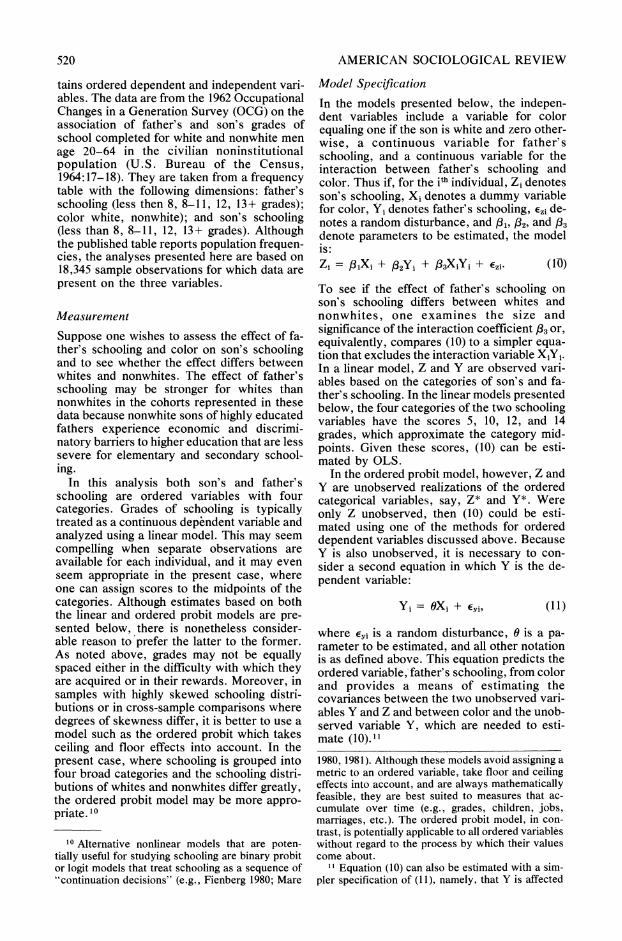
tains ordered dependent and independent variables. The data are from the 1962 Occupational Changes in a Generation Survey (OCG) on the association of father's and son's grades of school completed for white and nonwhite men age 20-64 in the civilian noninstitutional population (U.S. Bureau of the Census, 1964:17-18). They are taken from a frequency table with the following dimensions: father's schooling (less then 8, 8-11, 12, 13+ grades); color white, nonwhite); and son's schooling (less than 8, 8-11, 12, 13+ grades). Although the published table reports population frequencies, the analyses presented here are based on 18,345 sample observations for which data are present on the three variables.

Measurement

Suppose one wishes to assess the effect of father's schooling and color on son's schooling and to see whether the effect differs between whites and nonwhites. The effect of father's schooling may be stronger for whites than nonwhites in the cohorts represented in these data because nonwhite sons of highly educated fathers experience economic and discrimi- natory barriers to higher education that are less severe for elementary and secondary schooling.

In this analysis both son's and father's schooling are ordered variables with four categories. Grades of schooling is typically treated as a continuous dependent variable and analyzed using a linear model. This may seem compelling when separate observations are available for each individual, and it may even seem appropriate in the present case, where one can assign scores to the midpoints of the categories. Although estimates based on both the linear and ordered probit models are presented below, there is nonetheless consider- able reason to prefer the latter to the former. As noted above, grades may not be equally spaced either in the difficulty with which they are acquired or in their rewards. Moreover, in samples with highly skewed schooling distributions or in cross-sample comparisons where degrees of skewness differ, it is better to use a model such as the ordered probit which takes ceiling and floor effects into account. In the present case, where schooling is grouped into four broad categories and the schooling distributions of whites and nonwhites differ greatly, the ordered probit model may be more appropriate. IO

Model Specification

In the models presented below, the independent variables include a variable for color equaling one if the son is white and zero otherwise, a continuous variable for father's schooling, and a continuous variable for the interaction between father's schooling and color. Thus if, for the ith individual, Zi denotes son's schooling, Xi denotes a dummy variable for color, Yi denotes father's schooling, Ezi denotes a random disturbance, and /3k, /2, and /3

denote parameters to be estimated, the model is:

Zi = /18Xi + p2Yi + /33XiYi ? Ezi (10)

To see if the effect of father's schooling on son's schooling differs between whites and nonwhites, one examines the size and significance of the interaction coefficient 3 or, equivalently, compares (10) to a simpler equation that excludes the interaction variable X1Yi. In a linear model, Z and Y are observed variables based on the categories of son's and father's schooling. In the linear models presented below, the four categories of the two schooling variables have the scores 5, 10, 12, and 14 grades, which approximate the category midpoints. Given these scores, (10) can be estimated by OLS.

In the ordered probit model, however, Z and Y are unobserved realizations of the ordered categorical variables, say, Z* and Y*. Were only Z unobserved, then (10) could be estimated using one of the methods for ordered dependent variables discussed above. Because Y is also unobserved, it is necessary to consider a second equation in which Y is the dependent variable:

Yi= oXi + Eyi, (11)

where Eyi is a random disturbance, 0 is a parameter to be estimated, and all other notation is as defined above. This equation predicts the ordered variable, father's schooling, from color and provides a means of estimating the covariances between the two unobserved variables Y and Z and between color and the unobserved variable Y, which are needed to estimate (10)."I

10 Alternative nonlinear models that are potentially useful for studying schooling are binary probit or logit models that treat schooling as a sequence of "continuation decisions" (e.g., Fienberg 1980; Mare

1980, 1981). Although these models avoid assigning a metric to an ordered variable, take floor and ceiling effects into account, and are always mathematically feasible, they are best suited to measures that ac- cumulate over time (e.g., grades, children, jobs, marriages, etc.). The ordered probit model, in contrast, is potentially applicable to all ordered variables without regard to the process by which their values come about.

1I Equation (10) can also be estimated with a simpler specification of (11), namely, that Y is affected


Estimnation

The results reported below are obtained through simultaneous estimation of (10) and (11) by maximum likelihood under the assumptions that El. and E, are uncorrelated and each follows a normal distribution. This procedure is an extension of methods discussed above for a single, ordinal independent variable. That is, ( 11) is estimated along with the reduced form of (10),

Z. ` 8X, + vi,

where 8 = 13 + 1320 + ?3:1Xj and v = E1 + /32E2

+ 8:3E,7Xl. In addition, two disturbance correlations are estimated, say pi and P2, for nonwhites and whites respectively. In terms of the parameters of (10) and (11), p = [32 and P2 =

/32 + 3:30. The maximum likelihood procedures described in the Appendix are used to obtain the reduced-form parameters 0, 8, pi, and P2, and from these are derived the structural parameters 0, 1i 132, and 1:3.

Results

Table 1 presents ordered probit and linear regression estimates for the effect of father's schooling and color on son's schooling for models with and without terms for interaction of father's schooling and color. The first and third columns of ihe table show that both the ordered probit and linear models indicate much higher levels of schooling for whites and for sons of more highly educated fathers. The probit and linear coefficients are not directly com- parable inasmuch as the former are measured in the scale of z-scores (inverse of the cumulative normal distribution), whereas the latter are measured in grades of school completed. Nonetheless the two models yield much the same results about the effects of the independent variables. To see this, note that one can rescale the probit coefficients for color and father's schooling to the same units as the linear regression coefficients. Given the category midpoints assumed in the regression analysis, the standard deviations of son's and father's schooling are 2.802 and 3.194 respectively. As reported in Table 1, the probit coefficient for color gives the difference between whites and nonwhites on a latent variable for son's schooling that has a standard deviation of one. Under the assumption that the latent vari-

able has the same standard deviation as assumed in the linear regression, the coefficient for color is 1.088 (0.386 x 2.802). The probit coefficient for father's schooling is the effect of a one standard deviation change in father's schooling on son's schooling in standard deviation units. If the schooling variables are assumed to have the same scale as in the regression, the coefficient for father's schooling is 0.379 (0.432 x 2.802/3.194). The ordered probit results also imply that the schooling categories are approximately equally spaced in the probit scale, as indicated by the roughly equal distances between adjacent thresholds.

The ordered probit and linear models, however, yield different results about a possible interaction effect of father's schooling and color on son s schooling. According to the ordered probit results, the effect of father's schooling on son's schooling is approximately 25 percent larger for white sons than for nonwhite sons (.436 vs. .344). Rescaling the probit coefficients to conform to the standard deviations for father's and son's schooling assumed in the linear regression models yields a similar race difference in the effect of father's schooling (.383 vs. .302). The test statistic for the interaction parameter and the one degree of freedom likelihood ratio chi-square statistic (90067-90047 = 20) are significant, even taking account of the complexity of the OCB sample. 12 For the linear model, in contrast, the interaction coefficient is insignificant and of opposite sign to that of the probit model.

This discrepancy between the ordered probit and linear regression findings results from the sensitivity of the regression model to the different skewness of the white and nonwhite schooling distributions. Under the assumptions

only by the random disturbance En. Although computationally feasible, this specification is tantamount to assuming that color and father's schooling are uncorrelated, and thus gives an unsatisfactory estimate for /,3. Parameter estimates for (I 1) are available from the authors on request.

12 Because these data derive from a frequency table, it is possible to compute a likelihood ratio chi-square statistic to assess the goodness of fit of the model. Under the saturated model, the log likelihood statistic is minus 21;n jklog(Puk), where n,jk is the number of observations in the ill category of father's schooling (i= 1,2,3,4), the jth category of son's schooling (j=1,2,3,4), and the kth color group (k=1,2); and Pijk is the proportion of the kth color group that is in the ith father's and jth son's schooling categories. For these data this statistic is 89727, implying a chi-square fit statistic for the model with the father's schooling-race interaction of 90047-89727=320 with 20 degrees of freedom, indi- cating a poor fit. A better-fitting model allows for more complex interactions between father's and son's schooling than the two correlation coefficients assumed here. More complex interactions can be included in the ordered probit model, albeit at the expense of more complex interpretations. The goodness-of-fit test is appropriate only when data come from a fixed table and cell frequencies are large.


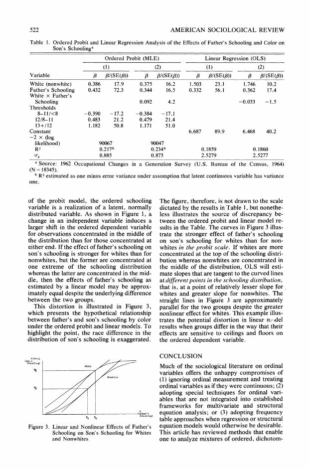
Table 1. Ordered Probit and Linear Regression Analysis of the Effects of Father's Schooling and Color on Son's Schoolinga

Ordered Probit (MLE) Linear Regression (OLS)

(1) (2) (1) (2) Variable 3 f8/(SE(/3)) /3 f/(SE(f)) 3 f8/(SE(f3)) / 8/(SE(f3))

White (nonwhite) 0.386 17.9 0.375 16.2 1.503 23.1 1.746 10.2 Father's Schooling 0.432 72.3 0.344 16.5 0.332 56.1 0.362 17.4 White x Father's

Schooling 0.092 4.2 -0.033 -1.5 Thresholds

8-11/<8 -0.390 -17.2 -0.384 -17.1 12/8-11 0.483 21.2 0.479 21.4 13+/12 1.182 50.8 1.171 51.0

Constant 6.687 89.9 6.468 40.2 -2 x (log

likelihood) 90067 90047 R2 0.217 b 0.234 b 0.1859 0.1860 0-e 0.885 0.875 2.5279 2.5277

a Source: 1962 Occupational Changes in a Generation Survey (U.S. Bureau of the Census, 1964) (N = 18345).

b R2 estimated as one minus error variance under assumption that latent continuous variable has variance one.

of the probit model, the ordered schooling variable is a realization of a latent, normally distributed variable. As shown in Figure 1, a change in an independent variable induces a larger shift in the ordered dependent variable for observations concentrated in the middle of the distribution than for those concentrated at either end. If the effect of father's schooling on son's schooling is stronger for whites than for nonwhites, but the former are concentrated at one extreme of the schooling distribution whereas the latter are concentrated in the middle, then the effects of father's schooling as estimated by a linear model may be approximately equal despite the underlying difference between the two groups.

This distortion is illustrated in Figure 3, which presents the hypothetical relationship between father's and son's schooling by color under the ordered probit and linear models. To highlight the point, the race difference in the distribution of son's schooling is exaggerated.

P(Y--J ) (S-'

SNhN'N1N~g)

Schoolin on Son's Schoolingfor

and N s Nonwhit

IrN YW Sc2hooling)

Figure 3. Linear and Nonlinear Effects of Father's Schooling on Son's Schooling for Whites and Nonwhites

The figure, therefore, is not drawn to the scale dictated by the results in Table 1, but nonetheless illustrates the source of discrepancy between the ordered probit and linear model results in the Table. The curves in Figure 3 illus- trate the stronger effect of father's schooling on son's schooling for whites than for nonwhites in the probit scale. If whites are more concentrated at the top of the schooling distribution whereas nonwhites are concentrated in the middle of the distribution, OLS will estimate slopes that are tangent to the curved lines at different points in the schooling distribution, that is, at a point of relatively lesser slope for whites and greater slope for nonwhites. The straight lines in Figure 3 are approximately parallel for the two groups despite the greater nonlinear effect for whites. This example illustrates the potential distortion in linear nr.,del results when groups differ in the way that their effects are sensitive to ceilings and floors on the ordered dependent variable.

CONCLUSION

Much of the sociological literature on ordinal variables offers the unhappy compromises of (1) ignoring ordinal measurement and treating ordinal variables as if they were continuous; (2) adopting special techniques for ordinal variables that are not integrated into established frameworks for multivariate and structural equation analysis; or (3) adopting frequency table approaches when regression or structural equation models would otherwise be desirable. This article has reviewed methods that enable one to analyze mixtures of ordered, dichotom-


ous, and continuous variables in structural equation models while taking account of the distinct measurement properties of these variables. Although the ordered logit and probit models are slightly more complex than multiple regression analysis inasmuch as they rely on nonlinear estimation methods, they can be implemented with standard statistical computer software. These methods require assumptions about the probability distributions of the unmeasured continuous variables from which ordered variables arise, but these assumptions are testable.

Like many topics in sociological methodology, the problem of ordinal variables has been discussed in isolation from broader methodological issues and with insufficient attention to high-quality research on the problem by applied statisticians in other fields. Whatever problems they may have presented methodologists, ordinal variables need present no special impediment to sound substantive research.

APPENDIX

Maximum Likelihood Estimation of Two-Equation Models with Ordinal Variables

As for single equations, maximum likelihood estimation for multiple equation models consists of specifying the probability of obtaining each observation as a function of the unknown parameters, forming the likelihood as the joint probability of obtaining all observations, and searching for parameter values that maximize the likelihood. Consider the two- equation model given by (6) and (7) above, but for simplicity assume again that 32 = 0. Then the reduced form of the model is given by (7) and (9). Further, assume that Y and Z follow a bivariate normal distribution, where Var(E,) = 0rEY and Var(v) = or . That is, the joint probability density function of the disturbances of the equations is

g (t,t) = [1(27r1- p)] x {exp[-(tY - 2ptyt, + t2)/(l - p2)]}, (Al)

where ty = Ey/orEy, tZ = v/c-,, and p denotes the correlation between Ey and v (e.g., Hogg and Craig, 1970). Given these assumptions it is possible to form the likelihood functions for alternative types of endogenous variables.

Suppose both Y and Z are unmeasured continuous variables that correspond to observed ordinal variables Y* and Z* respectively. That is, let aso, asi,-. asi-1 aSJ denote thresholds in the distribution of Y and Z (s = 1,2), where aso = _x, 9asJ = o,Y* = j if aii-1

- Y < a:j, and Z* = j' if a2i'-1 < Z < aS2j- To identify the scales of Y and Z assume that 0rEy = cry = 1. Then the probability of obtaining an observation with category j of Y* and j' of Z* is:

P(Y*l = j Z*, = j'iX1i) =

Jc1' iC2J' g (tZ19 ty1) dtzdtyg (A2) Clj-1 C2J'-1

where c1j = a1i-61Xij and c2P = a2i, - 81X1i. Then the likelihood function is:

L = [I [I [I [p(Y* = j, Z*, = j' X 1)] ijj (A3) i j j'

where dijj, is a variable that equals one if Y* = j and Z- j' and zero otherwise. Iterative estimation procedures pick 06, 81, and the acj that make L as large as possible.

If either Y* or Z* is a dichotomous variable, then the likelihood is just a special case of (A3), where one of the variables has only two ordered categories.

If Y is an unmeasured continuous variable corresponding to an observed ordinal variable Y*, but Z is an observed continuous variable, then no longer assume o-, = 1, but rather that o-, can be estimated from the data and that t, = (Zi - 81X1i)/o-v. Then the likelihood is:

Cjjd L = [I [I f [g (t, ty1) dt7 dty] ' (A4)

W lj-1

where dij is a variable that equals one if Y*, equals j, and zero otherwise.

Statistical Programs for Ordered Probit and Logit

Single equations with ordinal dependent variables can be estimated with "user-defined" functions in a number of commonly used statistical programs. In most of these programs, the user supplies the for- mula for the appropriate likelihood function and initial values for the estimated parameters. Initial values can be obtained using the dichotomous-variable approach discussed in this article or by ordinary least squares.

GLIM (Baker and Nelder, 1978), BMDP (Dixon, 1983), SAS (SAS Institute Inc., 1982), SPSSX (SPSS Inc., 1983), LIMDEP (Greene, n.d.), and HOTZTRAN (Avery and Hotz, 1983) permit the user to specify the ordered logit or probit likelihood functions and to estimate these models by maximum likelihood or its equivalent. LIMDEP and HOTZTRAN can also estimate ordered probit models directly without user specification of the likelihood function. Routines for estimating ordered probit models in BMDP or through a FORTRAN pro- gram that can be run on an IBM personal computer are available from the authors.'3 HOTZTRAN can also estimate models with multiple equations, ordered independent variables, latent variables with several ordinal indicators, and structural equation models with mixtures of continuous, discrete, ordinal, and truncated variables.'4

REFERENCES

Agresti, Alan 1983 "A survey of strategies for modeling cross-

classifications having ordinal variables."

13 This offer expires one year after publication of this article.

14 HOTZTRAN is available from Mathematica Policy Research.


Journal of the American Statistical Associ- ation 78:184-98.

Aitchison, J. and S. D. Silvey 1957 "The generalization of probit analysis to the

case of multiple responses." Biometrika 57:253-62.

Allan, G. J. B. 1976 "Ordinal-scaled variables and multivariate

analysis: comment on Hawkes." American Journal of Sociology 81:1498-1500.

Amemiya, Takeshi 1975 "Qualitative response models." Annals of

Economic and Social Measurement 4:363-72.

Aranda-Ordaz, F. J. 1981 "Two families of transformations to ad-

ditivity for binary response data." Biomet- rika 68:357-63.

Ashford, J. R. 1959 "An approach to the analysis of data for

semi-quantal responses in biological assay." Biometrics 15:573-81.

Avery, Robert B. and V. Joseph Hotz 1982 "Estimation of multiple indicator multiple

cause models with discrete indicators." Discussion Paper 82-7, Economics Re- search Center/NORC, University of Chicago.

1983 "HOTZTRAN User's Manual, Version 1.1." Unpublished Manuscript, Economics Research Center/NORC, University of Chicago.

Baker, R. J. and J. A. Nelder 1978 The GLIM System. Release 3. Generalized

Linear Interactive Modelling. Oxford: Royal Statistical Society.

Berk, Richard A. 1983 "An introduction to sample selection bias in

sociological data." American Sociological Review 48:386-98.

Bielby, William T. and Robert M. Hauser 1977 "Structural equation models." Annual Re-

view of Sociology 3:137-61. Blalock, Hubert M.

1974 Measurement in the Social Sciences: Theories and Strategies. Chicago: Aldine.

Bollen, Kenneth A. and Kenney H. Barb 1981 "Pearson's R and coarsely categorized

measures." American Sociological Review 46:232-39.

1983 "Collapsing variables and validity coefficients (reply to O'Brien)." American Sociological Review 48:286.

Borgatta, Edgar 1968 "My student, the purist: a lament."

Sociological Quarterly 9:29-34. Bradley, Edwin L.

1973 "The equivalence of maximum likelihood and weighted least squares estimates in the exponential family." Journal of the Ameri- can Statistical Association 68:199-200.

Clogg, Clifford C. 1982 "Using association models in sociological

research: some examples." American Jour- nal of Sociology 88:114-34.

Cox, D. R. 1970 The Analysis of Binary Data. London:

Methuen.

Dixon, W. J. 1983 BMDP Statistical Software. Berkeley: Uni-

versity of California Press. Featherman, David L. and Robert M. Hauser

1978 Opportunity and Change. New York: Aca- demic Press.

Fienberg, Stephen E. 1980 The Analysis of Cross-Classified Categori-

cal Data. Second edition. Cambridge, MA: MIT Press.

Gallant, A. Ronald 1975 "Nonlinear regression." The American

Statistician 29:73-81. Goldberger, Arthur S. and Otis Dudley Duncan

(eds.) 1973 Structural Equation Models in the Social

Sciences. New York: Seminar Press. Goodman, Leo A.

1980 "Three elementary views of log linear models for the analysis of cross-classifications having ordered categories." Pp. 193-239 in Samuel Leinhardt (ed.), Sociological Meth- odology 1981. San Francisco: Jossey-Bass.

Greene, William H. n.d. "LIMDEP: Estimator for limited and qual-

itative dependent variable models and sample selectivity models." Unpublished manuscript, Graduate School of Business Ad- ministration, New York University.

Gurland, John, Ilbok Lee and Paul A. Dahm 1960 "Polychotomous quantal response in

biological assay." Biometrics 16:382-98. Hanushek, Eric A. and John E. Jackson

1977 Statistical Methods for Social Scientists. New York: Academic Press.

Hawkes, Roland K. 1971 "The multivariate analysis of ordinal mea-

sures." American Journal of Sociology 76:908-26.

Heckman, James J. 1978 "Dummy endogenous variables in a simul-

taneous equation system." Econometrica 46:931-59."

1979 "Sample selection bias as a specification error." Econometrica 47:153-61.

Henry, Frank 1982 "Multivariate analysis and ordinal data."

American Sociological Review 47:299-304. Hogg, Robert V. and Allen T. Craig

1970 Introduction to Mathematical Statistics. Third edition. London: Macmillan.

Jencks, Christopher et al. 1979 Who Gets Ahead? The Determinants of

Success in America. New York: Basic. Jennrich, Robert I. and Roger H. Moore

1975 "Maximum likelihood by means of nonlinear least squares." Pp. 57-65 in Pro- ceedings of the Statistical Computing Sec- tion of the American Statistical Associa- tion. Washington, D.C.: American Statisti- cal Association.

Johnson, David R. and James C. Creech 1983 "Ordinal measures in multiple indicator

models: a simulation study of categoriza- tion error." American Sociological Review 48:398-407.


Johnson, Norman and Samuel Kotz 1970 Continuous Univariate Distributions-1.

New York: Wiley. Johnston, J.

1972 Econometric Methods. Second edition. New York: McGraw-Hill.

Kim, Jae-On 1975 "Multivariate analysis of ordinal vari-

ables." American Journal of Sociology 81:261-98.

1978 "Multivariate analysis of ordinal variables revisited." American Journal of Sociology 84:448-56.

Labovitz, Sanford 1967 "Some observations on measurement and

statistics." Social Forces 46:151-60. 1970 "The assignment of numbers to rank order

categories." American Sociological Review 35:515-24.

Maddala, G. S. 1983 Limited-Dependent and Qualitative Vari-

ables in Econometrics. Cambridge: Cam- bridge University Press.

Mare, Robert D. 1980 "Social background and school continua-

tion decisions." Journal of, the American Statistical Association 75:295-305.

1981 "Change and stability in educational stratification." American Sociological Re- view 46:72-87.

Mayer, Lawrence S. and Jeffrey A. Robinson 1978 "Measures of association for multiple re-

gression models with ordinal predictor variables." Pp. 141-63 in Karl F. Schuessler (ed.), Sociological Methodology 1978. San Francisco: Jossey-Bass.

McCullagh, Peter 1980 "Regression models for ordinal data."

Journal of the Royal Statistical Society, Series B 42:109-42.

McKelvey, Richard D. and William Zavoina 1975 "A statistical model for the analysis of ordi-

nal level dependent variables." Journal of Mathematical Sociology 4:103-20.

Morris, R. 1970 "Multiple correlation and ordinally scaled

data." Social Forces 48:299-311. Muthen, Bengt

1979 "A structural probit model with latent variables." Journal of the American Statistical Association 74:807-11.

1983 "Latent variable structural equation modeling with categorical data." Journal of Econometrics 22:43-65.

1984 "A general structural equation model with dichotomous, ordered categorical, and continuous latent variable indicators." Psychometrika 49:115-32.

Nelder, J. A. and R. W. M. Wedderburn 1972 "Generalized linear models." Journal of the

Royal Statistical Society, Series A, Part 3:370-84.

O'Brien, Robert M. 1979a "The use of Pearson's R with ordinal data."

American Sociological Review 44:851-57. 1979b "On Kim's 'multivariate analysis of ordinal

variables.' " American Journal of Sociology 85:668-69.

1981 "The relationship between ordinal measures and their underlying values: why all the disagreement?" Paper presented to the Annual Meetings of the American Sociological Association, Toronto, Canada.

1982 "Using rank-order measures to represent continuous variables." Social Forces 61:144-55.

1983 "Rank order versus rank category measures of continuous variables." American Sociological Review 48:284-86.

Pregibon, Daryl 1980 "Goodness of link tests for generalized

linear models." Applied Statistics 29:15-24. Reynolds, H.

1973 "On 'the multivariate analysis of ordinal measures.' " American Journal of Sociol- ogy 78:1513-16.

SAS Institute Inc. 1982 SAS User's Guide: Basics. 1982 Edition.

Cary, NC: SAS Institute Inc. SPSS Inc.

1983 SPSSX User's Guide. New York: McGraw-Hill.

Smith, Robert B. 1974 "Continuities in ordinal path analysis." So-

cial Forces 53:200-29. Somers, Robert H.

1974 "Analysis of partial rank correlation measures based on the product-moment model: part one." Social Forces 53:229-46.

Stinchcombe, Arthur 1983 "Linearity in loglinear analysis." Pp.

104-25 in Samuel Leinhardt (ed.), Sociological Methodology 1983-1984. San Francisco: Jossey-Bass.

U. S. Bureau of the Census 1964 "Education change in a generation March

1962." Current Population Reports Series P-20, No. 132. Washington, D.C.: U.S. Government Printing Office.

White, Halbert 1981 "Consequences and detection of

misspecified nonlinear regression models." Journal of the American Statistical Associ- ation 76:419-33.

Winship, Christopher and Robert D. Mare 1983 "Structural equations and path analysis for

discrete data." American Journal of Sociol- ogy 89:54-110.

regression models with ordinal...

Documents