Regression Models for Time Trends:

A Second ExampleINSR 260, Spring 2009

Bob Stine

1

Overview Resembles prior textbook occupancy example

Time series of revenue, costs and sales at Best Buy,in millions of dollarsQuarterly from 1995-2008

Similar featuresLog transformationSeasonal patterns via dummy variablesTesting for autocorrelation: Durbin-Watson, lag residualsPrediction with autocorrelation adjustments

Novel featuresUse of segmented model to capture change of regimeDecision to set aside some data to get consistent form

2

Forecasting ProblemPredict revenue at Best Buy for next year

Q1, 1995 through Q1, 200853 quartersForecast revenue for the rest of 2008Estimate forecast accuracy

Evident patternsGrowthSeasonalVariation

Forecast of profit needs an estimate of cost of goods sold and amount of sales: then difference.

3

$0.00

$2,500.00

$5,000.00

$7,500.00

$10,000.00

$12,500.00

$15,000.00

Revenue

1996 1998 2000 2002 2004 2006 2008

Time

Overlay Plot

Initial ModelingQuadratic trend + quarterly seasonal pattern

Overall fit is highly statistically significant

Nonetheless model shows problems in residuals

Trend in the first quarter of each year (red) appears different from those in other quarters… interaction.

4

RSquare

RSquare Adj

Root Mean Square Error

Mean of Response

Observations (or Sum Wgts)

0.959712

0.955426

632.221

4952.975

53

Summary of Fit

-1500

-1000

-500

0

500

1000

1500

2000

Revenue R

esid

ual

0 2500 5000 7500 12500

Revenue Predicted

Residual by Predicted Plot

-1500

-1000

-500

0

500

1000

1500

2000

Resid

ual

0 10 20 30 40 50 60

Row Number

Residual by Row Plot

Two Ways to FixTwo approaches

Add interactions that allow slopes to differ by quarterDo you want to predict quadratic growth?

Log transformation

Use logCurvature remains, but variance seems stable with consistent patterns in the quarters

5

1000

10000

8000

7000

6000

5000

4000

3000

2000

20000

Revenue

1996 1998 2000 2002 2004 2006 2008

Time

Overlay Plot

Model on Log ScaleModel of logs on time and quarter is highly statistically significant,

But residuals show lack of fit and dependence

Why does slope (% growth rate) seem to change?

6

RSquare

RSquare Adj

Root Mean Square Error

Mean of Response

Observations (or Sum Wgts)

0.987077

0.986

0.073872

8.324368

53

Summary of Fit

Intercept

Time

Quarter[1]

Quarter[2]

Quarter[3]

Term

-298.6066

0.1533451

0.2856838

-0.164648

-0.09888

Estimate

5.316919

0.002656

0.02846

0.029005

0.028982

Std Error

48.00

48.00

48.00

48.00

48.00

DFDen

-56.16

57.73

10.04

-5.68

-3.41

t Ratio

<.0001*

<.0001*

<.0001*

<.0001*

0.0013*

Prob>|t|

Indicator Function Parameterization

-0.20

-0.15

-0.10

-0.05

0.00

0.05

0.10

0.15

0.20

Log R

evenue

Resid

ual

7.0 7.5 8.0 8.5 9.0 9.5

Log Revenue Predicted

Residual by Predicted Plot

-0.20

-0.15

-0.10

-0.05

0.00

0.05

0.10

0.15

0.20

Resid

ual

0 10 20 30 40 50 60

Row Number

Residual by Row Plot

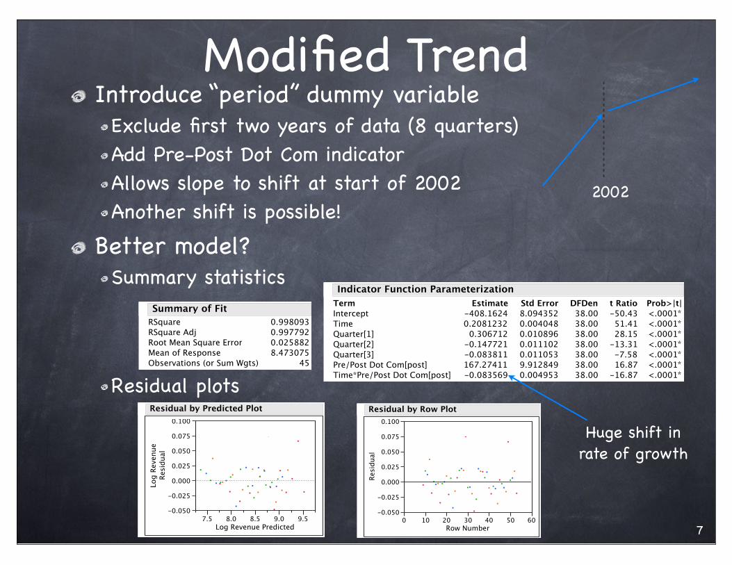
Modified TrendIntroduce “period” dummy variable

Exclude first two years of data (8 quarters)Add Pre-Post Dot Com indicatorAllows slope to shift at start of 2002Another shift is possible!

Better model?Summary statistics

Residual plots

7

2002

RSquare

RSquare Adj

Root Mean Square Error

Mean of Response

Observations (or Sum Wgts)

0.998093

0.997792

0.025882

8.473075

45

Summary of FitIntercept

Time

Quarter[1]

Quarter[2]

Quarter[3]

Pre/Post Dot Com[post]

Time*Pre/Post Dot Com[post]

Term

-408.1624

0.2081232

0.306712

-0.147721

-0.083811

167.27411

-0.083569

Estimate

8.094352

0.004048

0.010896

0.011102

0.011053

9.912849

0.004953

Std Error

38.00

38.00

38.00

38.00

38.00

38.00

38.00

DFDen

-50.43

51.41

28.15

-13.31

-7.58

16.87

-16.87

t Ratio

<.0001*

<.0001*

<.0001*

<.0001*

<.0001*

<.0001*

<.0001*

Prob>|t|

Indicator Function Parameterization

-0.050

-0.025

0.000

0.025

0.050

0.075

0.100

Log R

evenue

Resid

ual

7.5 8.0 8.5 9.0 9.5

Log Revenue Predicted

Residual by Predicted Plot

-0.050

-0.025

0.000

0.025

0.050

0.075

0.100

Resid

ual

0 10 20 30 40 50 60

Row Number

Residual by Row Plot

Huge shift in rate of growth

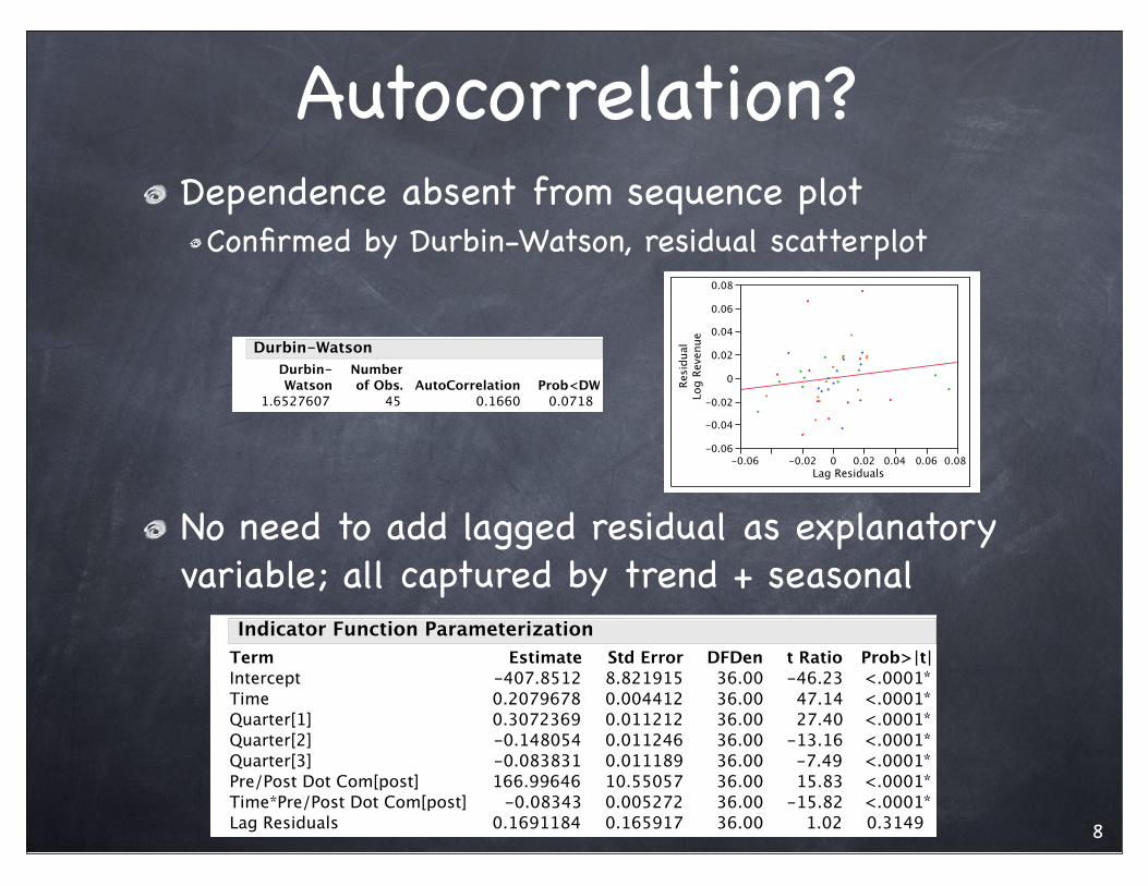
Autocorrelation?Dependence absent from sequence plot

Confirmed by Durbin-Watson, residual scatterplot

No need to add lagged residual as explanatory variable; all captured by trend + seasonal

8

1.6527607

Durbin-

Watson

45

Number

of Obs.

0.1660

AutoCorrelation

0.0718

Prob<DW

Durbin-Watson

-0.06

-0.04

-0.02

0

0.02

0.04

0.06

0.08

Resid

ual

Log R

evenue

-0.06 -0.02 0 0.02 0.04 0.06 0.08

Lag Residuals

Intercept

Time

Quarter[1]

Quarter[2]

Quarter[3]

Pre/Post Dot Com[post]

Time*Pre/Post Dot Com[post]

Lag Residuals

Term

-407.8512

0.2079678

0.3072369

-0.148054

-0.083831

166.99646

-0.08343

0.1691184

Estimate

8.821915

0.004412

0.011212

0.011246

0.011189

10.55057

0.005272

0.165917

Std Error

36.00

36.00

36.00

36.00

36.00

36.00

36.00

36.00

DFDen

-46.23

47.14

27.40

-13.16

-7.49

15.83

-15.82

1.02

t Ratio

<.0001*

<.0001*

<.0001*

<.0001*

<.0001*

<.0001*

<.0001*

0.3149

Prob>|t|

Indicator Function Parameterization

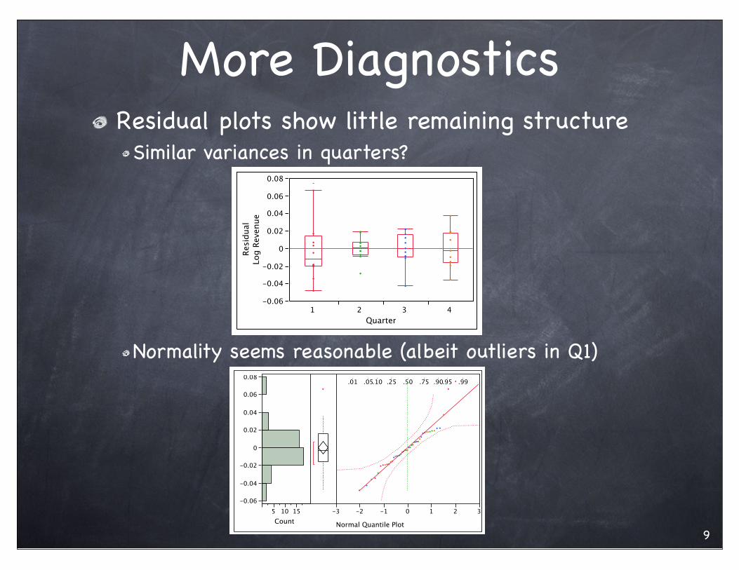
More DiagnosticsResidual plots show little remaining structure

Similar variances in quarters?

Normality seems reasonable (albeit outliers in Q1)

9

-0.06

-0.04

-0.02

0

0.02

0.04

0.06

0.08

Resid

ual

Log R

evenue

1 2 3 4

Quarter

-0.06

-0.04

-0.02

0

0.02

0.04

0.06

0.08

5 10 15

Count

.01 .05.10 .25 .50 .75 .90.95 .99

-3 -2 -1 0 1 2 3

Normal Quantile Plot

ForecastingForecast log revenue for rest of 2008ŷn+j = (-408.162 + 167.274 + Qj) + " " " " " seasonal" " (0.20812-0.08357) time" " time trendOverall intercept plus adjustment for pre/post

Examples for Q2, Q3, Q4 of 2008ŷ53+1 = (-408.162 + 167.274 - 0.148)" " " " Q2 = -0.148" " + 0.12455 (2008.25) " " ≈ 9.092ŷ53+2 = (-408.162 + 167.274 - 0.084)" " " Q3 = -0.100" " + 0.1245 (2008.50)" " ≈ 9.187ŷ53+3 = (-408.162 + 167.274)"" " " " " " Q4 = 0" " + 0.1245 (2008.75)" " ≈ 9.302

10

Forecast AccuracySince model does not have autocorrelation and data meet assumptions of MRM, we can use the JMP prediction intervals

One period outŷ53+1 ± t.025 SE(indiv pred) = 9.0415 to 9.1587

Two periods outŷ53+2±t.025 SE(indiv pred) = "9.1363" 9.2540

Three periods outŷ53+3±t.025 SE(indiv pred) = "9.2510" 9.3692

11

Prediction IntervalsObtain predictions of revenue, not the log of revenue

ConversionForm interval as we have done on transformed scaleExponentiate

" " 9.0415 to 9.1587" " ⇒"" e9.0415 to e9.1587

" " " " " " " " " " " " $8446 to $9497 (million)

As in prior example, the prediction interval is much wider than you may have expected from the R2 and RMSE of the model on the log scale.

Small differences on log scale are magnified on $ scale

12

Alternative SegmentsPrior approach adds two variables to segment

Dummy variable for period allows new interceptInteraction allows slope to change

Models fit in the two periods are “disconnected”Not constrained to be continuous or intersect where the second period begins

Alternative approach forces continuityAdd one parameter for change in the slopeNo dummy variable needed. Intercept defined by the location of the prior fit.

13Pre Post

Building the VariablesModel comparison

Break in structure (kink) at time TBefore (t ≤ T) : Yt = β0 + β1 Xt + εtAfter (t > T) : Yt = α0 + (β1 + δ)Xt + εt Choose α0 so that means match at time T" β0 + β1 XT"= α0 + (β1 + δ)XT ⇒ α0 = β0 - δXT

Hence, only need to estimate one parameter, δ

To fit with regression, add the variable Zt Zt = 0 for t≤T, Zt = Xt - XT for t > TBefore T: no effect on the fit since 0After T: β0 + β1 Xt + δ Zt = β0 + β1 Xt + δ (Xt - XT)" " " " " " " " " = (β0 - δXT) + (β1+δ) Xt

14

Changing the SlopeAdded variable is very simple

Prior to the change point, it’s 0After the change point, its (x - time of change)

Picture shows “dog-leg” shape of new variable with kink at the change point

15

NewVariable

ExampleFit with distinct segments

Fit with continuous jointAlmost as large R2, with one less estimated parameterSimilar shift in slope in two models.

16

RSquare

RSquare Adj

Root Mean Square Error

Mean of Response

Observations (or Sum Wgts)

0.997901

0.997632

0.026804

8.473075

45

Summary of Fit

RSquare

RSquare Adj

Root Mean Square Error

Mean of Response

Observations (or Sum Wgts)

0.998093

0.997792

0.025882

8.473075

45

Summary of FitIntercept

Time

Quarter[1]

Quarter[2]

Quarter[3]

Pre/Post Dot Com[post]

Time*Pre/Post Dot Com[post]

Term

-408.1624

0.2081232

0.306712

-0.147721

-0.083811

167.27411

-0.083569

Estimate

8.094352

0.004048

0.010896

0.011102

0.011053

9.912849

0.004953

Std Error

38.00

38.00

38.00

38.00

38.00

38.00

38.00

DFDen

-50.43

51.41

28.15

-13.31

-7.58

16.87

-16.87

t Ratio

<.0001*

<.0001*

<.0001*

<.0001*

<.0001*

<.0001*

<.0001*

Prob>|t|

Indicator Function Parameterization

Intercept

Time

Time Post

Quarter[1]

Quarter[2]

Quarter[3]

Term

-397.4332

0.2027556

-0.081303

0.3042508

-0.149787

-0.084844

Estimate

6.166522

0.003083

0.004988

0.011209

0.011446

0.011433

Std Error

39.00

39.00

39.00

39.00

39.00

39.00

DFDen

-64.45

65.76

-16.30

27.14

-13.09

-7.42

t Ratio

<.0001*

<.0001*

<.0001*

<.0001*

<.0001*

<.0001*

Prob>|t|

Indicator Function Parameterization

Summary A basic trend (linear, perhaps quadratic) plus dummy variables is a good starting model for many time series that show increasing levels.Log transformations stabilize the variation, are easily interpreted, and avoid more complicated trends and interactions.Dummy variables can model a “trend break”.

Models do not anticipate the time of another trend break in the future.Special “broken line” variable models shift in slope with one parameter, forcing continuity.

R2 is misleading when you see the prediction intervals when fitting on a log scale.

17