regional income dispersion and market potential in …eprints.lse.ac.uk/22311/1/wp106schulze.pdf ·...
TRANSCRIPT
Working Papers No. 106/07
Regional Income Dispersion and Market Potential in the Late
Nineteenth Century Hapsburg Empire
Max Stephan Schulze
© Max-Stephan Schulze
London School of Economics
November 2007

Department of Economic History London School of Economics Houghton Street London, WC2A 2AE Tel: +44 (0) 20 7955 7860 Fax: +44 (0) 20 7955 7730

Regional Income Dispersion and Market Potential in the Late
Nineteenth Century Habsburg Empire∗
Max-Stephan Schulze
Abstract This paper presents new regional GDP estimates for the Habsburg Monarchy and constructs measures of market potential for its 22 major regions. The paper argues that regional income differentials were significantly larger, that intra-empire catching-up of poor with rich regions was far more limited and that the empire’s Eastern regions were much further behind Western Europe than suggested in the historiography. The measurement of regional market potential proves strongly sensitive to the composition of foreign economies considered in the computations and the choice of regional ‘nodes’. Further, though being ‘remote’ imposed some penalty, there was no uniform relationship between changes in regions’ relative GDP position and their market potential.
1. Introduction
The profound regional differences in geography, resource
endowments and income across Austria-Hungary and issues of regional
division of labour are recurrent themes in the Habsburg historiography
(Good 1984; Gross 1973; Freudenberger, 2003; Komlos 1983). In the
1990s, David Good made a persistent effort to quantify regional product in
the Habsburg domains as a means to assess the economic lag of East-
Central Europe (Good 1991, 1994, 1997; Good and Ma 1998). According to
the 1998 estimates, the poorest region in Austria-Hungary enjoyed per
capita incomes that on the eve of the First World War, and after a long
process of industrialization in the western regions stretching back to the late
∗ I would like to thank the Economic and Social Research Council for financial support (grant RES-000-22-1598), Felipe Tamega Fernandes for research assistance and Dudley Baines for helpful comments.

18th century (good 1984; Komlos 1983, 1989), were about 60 per cent below
that of the richest region and about 30 per cent below the mean of the
empire. In the Habsburg case, as elsewhere in Europe, the timing, direction
and pace of economic change and industrialization were shaped by regional
conditions (Pollard 1986). Yet a theoretically explicit and quantitative
analysis of how these factors mattered for the development of the Habsburg
economy, and more broadly, Europe’s Eastern and South-Eastern periphery,
is still missing. This paper aims at providing some empirical input as a first
step towards such an analysis.
In terms of GDP per capita, the pre-1913 Austrian economy ranked
near the bottom of the European growth league: income rose by less than 1
per cent per annum. By contrast, in Hungary – Austria’s partner in the
Habsburg customs union – per capita product increased by about 1.3 per
cent during 1870-1913, (Schulze 2000, 2007). The following sections
present new (Austria) and revised (Hungary) GDP estimates for the 22 major
Habsburg regions as a means of gauging the extent to which empire-wide
aggregate product measures mask significant regional variations in levels of
economic activity. Further, they provide an input for the analysis of regional
differences as a potential source of Austria’s poor comparative growth
performance. Finally, the regional product estimates are a key ingredient in
the computation of regional market potential as an indicator of a region’s
centrality. The guiding idea from location theory is that producers are likely
to settle in those locations that offer the best (least costly) access to input
(supply) and output (demand) markets (Midelfart-Knarvik et al. 2000).
In an essentially descriptive exercise, the estimates for GDP and
market potential are used to address three issues. First, what was the extent
of regional income differentials across the 22 major regions of the Habsburg
Empire and how did these differentials change over time? Second, what do
2

computations of economic potential reveal about the centrality or
‘peripherality’ of the Habsburg regions? Third, to what extent did differences
in regional economic performance reflect differences in regional economic
potential?
2. Methods and Data
2.1 Estimating Regional GDP
Austrian regional GDP levels at constant 1913 prices and for 1870 to
1910 (at 10 year census intervals) have been built up from sector level
estimates, mirroring the procedure used in the construction of state-wide
aggregates (Schulze 2000). The fourteen regions include: Lower Austria,
Upper Austria, Salzburg, Styria, Carinthia, Carniola, Littoral,
Tyrol/Vorarlberg, Bohemia, Moravia, Silesia, Galicia, Bukovina and
Dalmatia. For Hungary, the paper relies on regional shares in total GDP
derived from Good and Ma (1998), applying them to Hungarian total product
(Schulze 2000, 2007). The estimates for Hungary cover eight regions: Left
Bank Danube, Right Bank Danube, Danube Tisza Basin, Right Bank Tisza,
Left Bank Tisza, Tisza Maros Basin, Transylvania and Croatia-Slavonia.
Good and Ma adopt a Crafts-type structural equation approach to
estimate regional per capita income levels as a function of several proxy
variables such as crude death rates, the share of the agricultural labour
force and letters posted (Crafts 1983; Good 1994). The procedure and its
application to the Habsburg case have been criticized by Pammer (1997) on
theoretical and empirical grounds, leading to significant revisions of the
estimates (Good, 1997; Good and Ma 1998). The proxy approach offers a
way to estimate regional income levels where standard national income
measures cannot be computed for lack of essential data. This, at present, is
3
the case for the Hungarian regions. For Austria, though, the sources allow
reconstructing regional GDP within a national income accounting framework
and from the output side. The key advantage compared to the earlier proxy
approach to derive regional GDP estimates is the use of variables and
measures that are theoretically linked to GDP. Section 3 below shows that
the choice of procedure makes for large differences in outcomes.
Crafts (2004, 2007) relies on a modified version of Geary and Stark
(2002) to estimate British regional GDP as a function of sectoral wages and
sectoral employment, augmented by the evidence from income tax returns to
account for the non-wage income component of GDP. Here a different route
was adopted. Regional GDPs were estimated for each sector separately,
reflecting the differences in data availability for each sector, by estimating
regional shares in sectoral output at the national level and then aggregating
across sectors (or industry branches) for each region. The national level
‘frame’ of sectoral gross value-added is provided in Schulze (2000, 2007).
For crop production this is straightforward as quantities of output for
more than twenty major products, valued at 1913 prices, are available from
Sandgruber (1978). The same source is used for estimating regional shares
in livestock output, using the detailed material that underlies the national-
level aggregates (Schulze 2000). Mining: regional quantities of the full range
of mining products and 1913 prices are readily available from the official
statistics (Bergbaustatistik). Regional shares in iron and steel production
have been approximated on the basis of regional output of pig iron and cast
iron (Huettenwesen). No data are available on the regional distribution of
wrought iron and steel output. However, the labour force statistics would
indicate that this introduces no undue bias as refining was concentrated in
the same regions as smelting (Austria – Census).
4
For manufacturing and construction the regional estimates build on
wage and employment data extracted from the statistics of the workers’
accident insurance system (Unfallstatistik). The data differentiate between
twelve major industry branches and about 38 sub-branches. For each
benchmark year and each industry branch, regional wage sums have been
converted into gross value added drawing on industry-specific wage
sum/output ratios and value-added proportions from Fellner (1916). In the
next step, gross value-added per worker was computed for each industry
branch in each region. Finally, and cognizant of the less than full coverage of
the accident insurance system, a region’s share in total output of a given
industry was computed by multiplying regional gross value-added per worker
by regional employment in that industry. The relevant regional industry-level
employment data have been taken from the censuses (Austria – Census).1
In the tertiary sector, regional shares in total gross value-added were
computed for trade, finance and communications and government,
professional and personal services on the basis of labour force statistics as
no other data are available (Austria – Census). In the case of the latter,
though, this corresponds fully with Kausel’s (1979) series, incorporated in
Schulze (2000), which provides the relevant ‘frame’ within which the regional
estimates slot. Finally, regional shares in total rental income from housing
have been estimated drawing on regional population and differences in
regional output per capita (with regional GDP per capita excluding rental
income as a proxy for average regional income).
1 For 1870 and 1880, regional shares in industrial output were computed on the basis of weighted 1890 regional output per worker relatives, 1870 (1880) overall industrial output per worker and 1870 (1880) regional industrial employment levels. The regional shares so derived were cross-checked against the material in NIHV and found consistent.
5
The new estimates are documented in Tables 4 to 6 below,
contrasting them with the results of Good and Ma’s (1998) earlier proxy
approach.
2.2 Estimating Market Potential
The market potential of a region depends on economic activity in that
region and in other adjacent or distant regions (or countries) adjusted for
their proximity. Proximity, in turn, depends on distance between localities
over land and sea. Distances over land and sea are converted into
equivalent measures using corresponding transport costs. Hence changes
over time in a region’s relative market potential can result from either shifts
in the spatial distribution of economic activity, changes in relative transport
cost or a combination thereof. Market potential can serve as a measure of a
region’s economic ‘centrality’ or ‘peripherality’. In the market access
literature (Midelfart-Knarvik et al. 2000), the degree of regions’ centrality is
expected to impact on firms’ location decisions – all else being equal,
producers are likely to locate where they find least costly access to markets
for their inputs and outputs.
Going back to Harris (1954), the market potential of region i (MPi) can
be calculated as increasing in purchasing power or GDP of all regions j
(GDPj) and decreasing in distance or transport cost between regions i and j
(Dij). This can be formulated as
MPi = Σj GDPj*Dγij
where γ is a distance weighting parameter set at –1. The regional market
potential calculations are augmented by an ‘own’ distance measure Dii.
(which is commonly approximated as a function of area size: Dii =
6

0.333√(areai/π))2 and the GDPs of the empire’s main trading partners with
the associated distance (or transport cost) measures.
Estimating market potential requires data on the GDP of domestic
regions and foreign countries, measures of transport costs and other trade
costs such as tariffs. New GDP estimates for the Habsburg regions are
documented in Table 4. GDP data for the empire’s main foreign trading
partners are taken from Maddison (2003), measured in purchasing power
parity adjusted international dollars.3 Fifteen foreign economies are included:
Belgium, Denmark, France, Germany, India, Italy, Netherlands, Portugal,
Russia, Spain, Sweden, Switzerland, Turkey, the United Kingdom and the
United States. However, almost three quarters of the empire’s foreign trade
was geared towards Continental Europe and more than half of that was with
Germany alone (ÖSH ).
With motorized road freight developing only after the First World War,
both the internal and external goods traffic of the Habsburg Empire was
heavily dominated by the railways. Coastal shipping played no significant
role in internal transport. In 1913, the volume of freight transported between
the empire’s Mediterranean ports accounted for half a per cent of freight
moved on the Austro-Hungarian railways (ÖSH, MSE). Likewise, waterborne
transport on the rivers Danube, Elbe and Vlatava, the only major inland
waterways, was equivalent to just one per cent of the railways’ ton-
2 The formula yields a distance value of 1/3 of the radius of a circle of the same area as region i. 3 In principle, the use current price GDP seems preferable to constant price-PPP adjusted GDP as in terms of location decisions that is what mattered to economic agents at the time. However, GDP deflators that would allow reflating the constant price estimates of Habsburg GDP are as yet not available (or rather, only very crude approximations would be possible at this stage). Further, the question of what determines the location of industry is not the primary issue under enquiry in this paper. Here the interest lies mainly in the ex-post comparison of inter-temporal changes in absolute and relative regional income and regional market potential.
7
kilometres. Accordingly, railways are chosen as the transport mode for
distances between the regions of the empire. Further, almost three quarters
of the empire’s foreign trade was geared towards Continental Europe and
more than half of that was with Germany alone (ÖSH) .
For distances between Habsburg regions and foreign countries, the
transport mode chosen was the cheaper of rail or rail and ship, based on
new estimates of time-varying railway freight rates for Austria-Hungary and
several European countries (see below) and Kaukiainen’s (2003) estimate of
ocean shipping rates. For both railway and sea transport cost
approximations, coal and grain were taken as representative cargoes (cf.
Crafts 2007). Further, both sets of freight rates build on estimates of terminal
charges and cost per ton-mile.
Distances. For the measurement of railway distances between
Habsburg regions and between these regions and foreign countries,
provincial and country capitals, respectively, have been chosen as the
relevant ‘nodes’. Both the domestic and the international railway connections
are measured such that they take full account of changes over time in route
length. Railway distance measures between the twenty-two Habsburg
internal ‘nodes’ have been extracted from the numerous sources listed under
Railway Distances. For connections from Habsburg to foreign ‘nodes’ (and
to/from port cities such as Hamburg, for example) the initial source is
Bradshaw’s 1914 Continental Guide. The distances reported there were
checked against (and augmented by additional distance measures from)
contemporary railway maps, held at the British Library, for all relevant years
prior to 1914. Whenever the 1914 connection was not in place before, the
shortest alternative route was extracted from this material.
Ocean shipping. The length of sea journeys has been estimated using
the material in www.dataloy.com/newwebsite/index.php; as mentioned
8
above, estimates of costs of ocean transport have been taken from
Kaukiainen (2003) and are reported in Table 1. Note, though, that only a
relatively small proportion (c. 12 per cent) of Austria-Hungary’s total foreign
trade was conducted through her Mediterranean ports and, likewise, the port
of Hamburg.
Railway freight cost. Estimates of railway transport cost are based on
material from a diverse set of sources. The (US) Bureau of Railway
Economics (1915) provides comparative 1914 freight rate data for a large
number of different-length railway routes in different countries and for a
variety of products. Again, as for sea transport, coal and grain were chosen
as representative cargoes. For both products transport costs were
decomposed into terminal and variable charges, providing a set of 1914
baseline estimates for Austria-Hungary and several other European
countries. Noyes (1905) and Cain (1980) provide estimates of average
railway freight rates per ton-mile for Austria-Hungary, France, Germany,
Italy, European Russia and Britain, respectively. These data have been
converted into indices and used to extrapolate back to 1870 both the
terminal and variable components in the 1914 equations. The estimates are
shown in Table 2. For rail connections within the Habsburg Empire the rates
reported under ‘Austria’ have been used, deflated by the ‘Generalindex’ of
Mühlpeck et al. (1979). For rail connections between the Habsburg regions
and foreign countries the arithmetic average of the Austrian and appropriate
foreign rates given in Table 2 has been used, again deflated. Where no
foreign country-specific freight rates are available for foreign countries, the
estimate for ‘Europe’ has been used instead.
The comparison of real cost of transport in Table 3 shows that ocean
freight rates fell more quickly over the course of the late nineteenth and early
twentieth centuries than railway freight rates. The implication here is, all else
9

being equal, that market potential increased relatively faster in those regions
of the empire that had ready access to the sea, like the Littoral (Trieste) and
Dalmatia, compared with landlocked regions like the Bukovina and Silesia.
Tariffs. The last building block for the estimation of market potential
involves accounting for the effects of trade costs such as tariffs. Here, the
procedure of Crafts and Mulatu (2006) was followed to convert tariffs into
distance equivalents drawing on Estevadeordal et al. (2003). They estimated
a gravity model for trade which has a distance elasticity of -0.8 and a tariff
elasticity of -1.0 (where the tariff is measured as (1+t)). These elasticities
have been used to convert ad valorem tariffs between any two given
countries into a distance equivalent measure which was then added to the
intercept of the equations for sea and rail freight rates reported in Tables 1
and 2. All tariff figures were computed as the ratio of customs revenue over
value of imports and Mitchell (2003) was the main source.4
Drawing on these elements (regional GDP, transport costs, tariffs),
market potential estimates for all 22 Habsburg regions are presented in
Tables 8 to 10, showing the evidence for three different country samples.
3. Growth and Dispersion in Regional Product The new regional GDP estimates for the Habsburg regions are
documented in Tables 4 and 5. They show major level differences compared
with the results of Good and Ma (1998), ranging between a minimum of +/- 1
per cent (Salzburg) and +/- 39 per cent (Dalmatia) for 1910. For the Austrian
4 Other sources are Mitchell and Deane for the UK; Prados de la Escosura (2003) for Spanish imports; Johanson (1984) for Denmark; Lains (2006) for Portuguese imports and Capie (1994) for an approximation of the German tariff rate for 1870.
10

part of the empire, these differences add up to 10 per cent and to about 13
per cent for the Hungarian half, also for 1910 (Table 6).5
Overall, regional product levels followed a far more pronounced profile
of variations than the earlier historiography suggests. In 1870, the richest
region (Lower Austria) enjoyed per capita incomes that were about 108 per
cent above the Habsburg average and about 240 per cent above the level of
the poorest region (Dalmatia). By 1910, this had changed to 74 and 258 per
cent, respectively. The coefficients of variation for all years show a
significantly higher degree of regional income dispersion for both Austria and
the Habsburg Empire as a whole than indicated by the results of the proxy-
approach (Table 5). All this suggest that the use of proxy variable within a
structural-equations framework masks the extent and persistence of regional
income differentials.
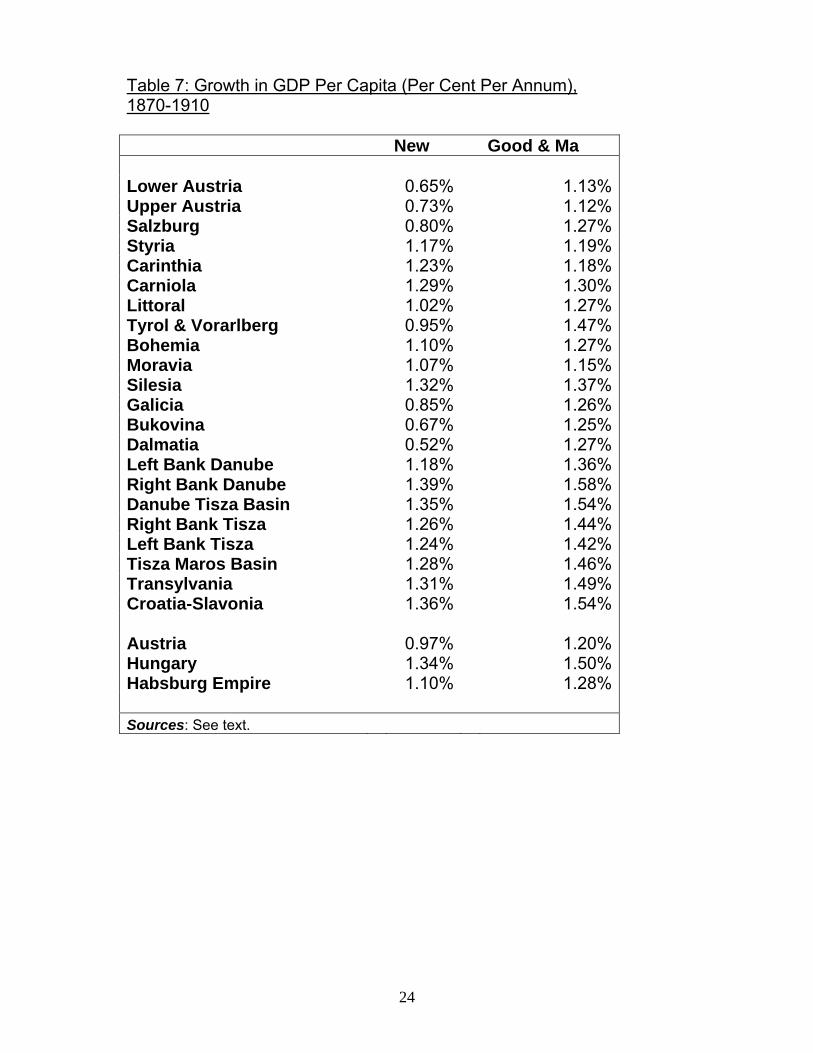
The material in Table 7 illustrates the extent of regional growth
variations and contrasts the new evidence with the findings of Good and Ma.
The key messages here is that growth in GDP per capita was persistently
slower across the regions and, at the same time, characterized by stark
inter-regional differences. Whereas the Good and Ma estimates for Austria
point to a fairly narrow range of regional growth between 1.12 (Upper
Austria) and 1.47 per cent per annum (Tyrol & Vorarlberg), the new
estimates suggest a far wider band between 0.52 (Dalmatia) and 1.32 per
cent (Silesia). Thus reconstructing regional GDP on the basis of regional
output and employment data yields estimates that seem far more responsive
to regional conditions and endowments.
5 Note that the regional GDP estimates for Hungary are based Good and Ma’s (1998) regional shares in total Hungarian GDP in each benchmark year that were applied to total state-level GDP as estimated in Schulze (2000, 2007) – the effect is an identical percentage point difference between the new and the Good and Ma estimates across all Hungarian regions in any given year. These differences, of course, change over time.
11

In Austria, the initially poorest regions in terms of GDP per capita in
the East and South-East (Galicia, Bukovina, Dalmatia) were expanding at as
low rates as the three richest regions in the West (Lower Austria, Upper
Austria, Salzburg). This ties in well with the slow decline in income
dispersion reported in Table 7. Apart from the generally faster growth of the
Hungarian regions compared with those in Austria, there is only very limited
evidence for intra-empire catching-up. Within the Austrian half of the
monarchy, it was the initially mid-income regions such as Bohemia and
Silesia whose relative position improved over 1870 to 1910.
4. Regional Market Potential in Austria-Hungary
Three alternative estimates of regional market potential have been
prepared. These show that the composition of the sample of foreign
countries included has a powerful influence on the Habsburg regions’
relative market potential (Tables 8-10).
According to the evidence in Table 8, the relative position of two
regions – the Littoral and Dalmatia – is particularly noteworthy. Their market
potential was the highest in 1870 and continued to rise the fastest up to
1910. In close proximity to sea routes they were well located to benefit from
lower and relatively fast declining shipping rates, offering ready access to
overseas markets. The effect, though, is somewhat exaggerated as the two
port cities of Trieste and Zara are the designated nodes. The only other
regions that saw significant change in their relative market potential were
Carniola adjacent to the Littoral, and Croatia-Slavonia – again, a region that
is bordering on the sea. For all other, landlocked, regions the relative market
potential remained practically unchanged over the period 1870 to 1910. In
12
other words, changes in railway route length and shifts in relative transport
costs (shipping vs. rail) had little effect.
Rather low and declining transport cost to India, the USA and Turkey
means that their GDPs feature strongly in the market potential measures,
particularly in coastal regions. However, the use of a foreign country sample
restricted to Europe reduces estimated relative market potential of the
regions. For landlocked regions far removed from ports such as the
Bukovina, Galicia and Transylvania, the inclusion or exclusion of these
economies makes no difference (Table 9). Bohemia’s profile is raised,
though. This is an outcome of her proximity to large economies such as
Germany and the UK (via the port of Hamburg) whose GDP now gains more
weight in the market potential calculations. This finding is consistent with the
foreign trade data: more than half of the empire’s foreign just before the First
World War was conducted with these two economies.
If the analysis is further restricted to consider only the GDP of the
Habsburg regions, the emerging picture is one of stasis (Table 10). In effect,
the procedure maximizes the impact of a region’s own potential and that of
its adjacent regions. There are no differential changes in transport costs over
time as railway freight rates are assumed to change at the same rate across
the entire network of the empire. Dalmatia, the region with the largest market
potential if the full sample were considered, turns into the region with the
lowest potential in the Habsburg-only setting. This is no coincidence. In fact,
Dalmatia was not only the poorest and least rapidly growing region of the
empire – it was also the only region with no direct railway connection to the
rest of the empire.
13

5. Some Preliminary Conclusions This paper has presented new estimates of regional GDP and regional
market potential in the Habsburg Empire. There are several conclusions.
First, regional differentials in terms of both levels and growth of per
capita GDP were significantly larger than earlier estimates based on the
proxy-approach suggest. Further, the Eastern parts of the empire were
economically much further behind Western Europe than the recent
historiography acknowledges.
Second, intra-empire catching-up of poor with rich regions was very
limited just as much as the Habsburg Empire, and especially Austria, failed
to catch-up with the leaders in the European income league. .
Third, the measurement of market potential is highly sensitive to the
composition of the group of foreign economies considered in the calculations
and the choice of ‘nodes’. Improvements in this area will involve the
generation of new regional income estimates for Germany as the empire’s
main trading partner, building on Frank (1994), to replace the German
aggregate. Further, drawing on overseas port cities as nodes (e.g. New
York, Bombay etc.) appears to bias the result by, effectively, lowering
relative transport cost. Hence the use of alternative, more ‘representative’
nodes needs to be explored. Likewise, the unique position of Dalmatia and
Zara as a node needs to be accounted for by, for instance, allowing for high-
cost road transport in the absence of direct rail communications.
Fourth, comparatively low and falling relative shipping cost meant that
regions close to the sea further improved their market potential relative to
landlocked regions during 1870 to 1910.
Fifth, some Habsburg regions commonly described in the literature as
‘remote’, ‘economically backward’ or ‘peripheral’ (e.g. the Bukovina and
Galicia) display low levels of market potential on all alternative measures.
14

Finally, there is no clear-cut relationship between changes in regions’
relative GDP (or GDP per capita) position and market potential. However,
some regions such as, for example, Silesia appear to have been far more
successful in tapping into their economic potential than others.
15

References
A. Official Publications, Maps, Reports, Statistics
Census 1869: K.k. Statistische Central-Commission, Bevölkerung und
Viehstand der im Reichsrathe vertretenen Königreiche und Länder,
dann der Militärgränze. Nach der Zählung vom 31. December 1869.
Heft II: Anwesende Bevölkerung nach Beruf und Beschäftigung
(Vienna, 1871).
Census 1880: K.k. Statistische Central-Commission, ‘Die Bevölkerung der
im Reichsrathe vertretenen Königreiche und Länder nach Beruf und
Erwerb’, Österreichische Statistik I (1882) 3. Heft.
Census 1890: K.k. Statistische Central-Commission, ‘Berufsstatistik nach
den Ergebnissen der Volkszählung vom 31. December 1890’,
Österreichische Statistik XXXIII (1894) 1. Heft ff..
Census 1910: K.k. Statistische Central-Commission ‘Berufsstatistik nach
den Ergebnissen der Volkszählung vom 31. Dezember 1910’,
Österreichische Statistik, N.F., III (1916) 1. Heft ff.
MSE: Magyar Kir. Központi Statisztikai Hivatal, Magyar Statisztikai Évkönyv,
1872-1915 (Budapest).
NIHV: Nachrichten über Industrie, Handel und Verkehr 1870, 1880 (Vienna:
1873, 1886).
ÖSH: k.k. Statistische Central-Commission, Österreichisches Statistisches
Handbuch, 1883-1915 (Vienna).
Railway Distances:
(a) Neueste Eisenbahnkarte der österreichischen Monarchie, C. Lehmann
(Vienna: 1870);
16

(b) Eisenbahn-Karte von Oesterreich-Ungarn, bearb. von T. Bomsdorff,
einschl. Kilometer-Zeiger fuer die Eisenbahnen Oesterreich-Ungarns
(Vienna: 1878);
(c) Oesterreich-Ungarn. Eisenbahn-Karte, gezeichnet und bearbeitet von T.
v. Bomsdorff (Vienna: 1883);
(d) Artaria’s Eisenbahn-, Post- und Communicationskarte von Oesterreich-
Ungarn (Vienna: 1888, 1891, 93, 1900).
(e) Eisenbahn- und Strassenkarte der oesterreichisch-ungarischen
Monarchie (Vienna: 1904).
(f) Uebersichtskarte der Eisenbahnen der oesterreichisch-ungarischen
Monarchie (Vienna: 1913).
(g) Artaria’s Eisenbahnkarte von Oesterreich-Ungarn, 3. Aufl., einschl.
Stations-verzeichnis, etc. (Vienna: 1913).
(h) A. Bechtel, Kilometerzeiger zu den allgemeinen und Militaer-Tarifen der
oesterreichisch-ungarischen Eisenbahnen (Vienna: 1882-91).
(i) F. Smolik, Offizieller Kilometerzeiger der saemtlichen oesterreichisch-
ungarischen und bosnisch-hercegovinischen Eisenbahnen (Vienna:
1912).
SJB: (1870-1882): k.k. Statistische Central-Commission, Statistisches
Jahrbuch der österreichischen Monarchie, 1870-1882 (Vienna).
Unfallstatistik: (a) K.k. Ministerium des Innern, Die Gebarung und die
Ergbenisse der Unfallstatistik 1889-1896 (Vienna, 1891-1898).
(b) K.k. Ministerium des Innern, Ergebnisse der Unfallstatistik der fünfjährigen
Beobachtungsperiode 1897-1901, 1902-1907, 1907-1911 (Vienna,
1904-1914).
(US) Bureau of Railway Economics (1915), Comparison of Railway Freight
Rates in the United States (and) The Principal Countries of Europe,
South Australia, and South Africa (Washington, D.C.).
17
B. Books, Articles
Abramovitz, M. (1986), ‘Catching up, forging ahead and falling behind’,
Journal of Economic History 46, No.2, pp.385-406.
Bradshaw’s August 1914 Continental Guide (repr. Newton Abbot, 1972)
Cain, P.J. (1980), ‘Private enterprise or public utility? Output, pricing and
investment on English and Welsh railways, 1870-1914’, Journal of
Transport History 1, No.1, pp.9-28.
Capie, F. (1994), Tariffs and Growth (Manchester 1994).
Crafts, N.F.R. (2005), ‘Regional GDP in Britain, 1871-1911: Some
estimates’, Scottish Journal of Political Economy 52, No.1, pp.54-64.
Crafts, N.F.R. and A. Mulatu (2006), ‘How did the location of industry
respond to falling transport costs in Britain before World War I?’,
Journal of Economic History 66, No.3, pp.575-607.
Estevadeordal, A., Frantz, B. and A. Taylor (2003), ‘The rise and fall of world
trade, 1870-1939’, Quarterly Journal of Economics 118, No.2, pp.359-
407.
Fellner, F. (1915), ‘Das Volksvermögen Österreichs und Ungarns’, Bulletin
de l’Institut International de Statistique, Tome XX – 2e Livraison
(Vienna), pp.503-573.
Frank, H. (1994), Regionale Entwicklungsdisparitäten im deutschen
Industrialisierungs-prozeß (Münster).
Freudenberger , H. (2003), Lost Momentum. Austrian Economic
Development 1750s-1830s (Vienna).
Gerschenkron, A. (1962), Economic Backwardness in Historical Perspective
(Cambridge, MA)
Estevadeordal, A., Frantz, B. and A. Taylor (2002), ‘The rise and fall of world
trade, 1870-1939’, NBER Working Paper No. 9318.
18

Geary, F. and T. Stark (2002), ‘Examining Ireland’s post-famine economic
growth performance’, Economic Journal 112, pp.919-35.
Good, D.F. (1984). The Economic Rise of the Habsburg Empire, 1750-1914
(Berkeley).
Good, D.F. (1994). ‘The economic lag of central and eastern Europe: income
estimates for the Habsburg successor states, 1870-1910’, Journal of
Economic History 54, No.4, pp.869-91.
Good, D.F. (1997). ‘ Proxy data and income estimates: reply to Pammer’,
Journal of Economic History 57, No.3, pp.456-63.
Good, D.F and Ma, T. (1998). ‘New estimates of income levels in central and
eastern Europe, 1870-1910’, in F. Baltzarek, F. Butschek and G. Tichy
(eds), Von der Theorie zur Wirtschaftspolitik - ein österreichischer Weg
(Stuttgart).
Harris, C. (1954), ‘The market as a factor in the localization of industry in the
United States’, Annals of the Association of American Geographers 64,
pp.315-348.
Johansen, H.C. (1980), Dansk historisk statistik (Copenhagen).
Kaukiainen, Y. (2003), ‘How the price of distance declined: Ocean freights
for grain and coal from the 1870s to 2000’, mimeo, University of
Helsinki.
Kausel, A. (1979), ‘Österreichs Volkseinkommen 1830 bis 1913’, in
Österreichisches Statistisches Zentralamt (ed.), Geschichte und
Ergebnisse der zentralen amtlichen Statistik in Österreich, 1829-1979
(Vienna), pp. 689-720.
Komlos, J. (1983). The Habsburg Monarchy as a Customs Union. Economic
Development in Austria-Hungary in the Nineteenth Century (Princeton).
19
Komlos, J. (1989). Stature, Nutrition, and Economic Development in the
Eighteenth Century Habsburg Monarchy: The `Austrian' Model of the
Industrial Revolution. (Princeton).
Lains, P. (2006), ‘Growth in a protected environment: Portugal, 1850-1950’,
Research in Economic History 24, pp.121-163.
Maddison, A. (2003), The World Economy: Historical Statistics (Paris).
Midelfart-Knarvik, K.H., H.G. Overman, S.J. Redding and A.J. Venables
(2000), ‘The location of European industry’, Economic Papers 142. DG
Economic and Financial Affairs, European Commission (Brussels).
Mitchell B.R. (2003), International Historical Statistics: Europe, 1750-2000
(Basingstoke).
Mirchell, B.R., Deane, P. (1962), Abstract of British Historical Statistics
(Cambridge).
Pammer, M. (1997). ‘Proxy data and income estimates: The economic lag of
central and eastern Europe’. Journal of Economic History 57, No.2,
pp.448-455.
Noyes, W.G. (1905), American Railroad Rates (Boston).
Pollard, S. (1986), Peaceful Conquest (reprint, Oxford).
Prados de la Escosura, L. (2000), ‘International comparisons of real product,
1820-1990: An alternative data set’, Explorations in Economic History
37, pp.1-41.
Prados de la Escosura, L.(2003), El progreso económico de España
(Madrid).
Sandgruber, R. (1978), Österreichische Agrarstatistik 1750-1918 (Munich).
Schulze, M.S. (2000), ‘Patterns of growth and stagnation in the late
nineteenth century Habsburg economy’, European Review of
Economic History 4, pp.311-340.
20

Schulze, M.S. (2007), ‘Origins of catch-up failure: comparative productivity
growth in the Habsburg Empire, 1870-1910’, European Review of
Economic History 11, pp.189-218.
21

22
Table 1: Shipping Rates Per Ton (current price in old pence) Terminal Component Cost per mile 1870 159 0.0461880 132 0.0301890 104 0.0201900 79 0.0181910 70 0.020Source: Kaukiainen (2003) . Years refer to 1872-1874, 1879-1880, 1888-1889, 1898-1899 and 1911-1913.
Table 2: Railway Freight Rates Per Ton (current price in old pence) Austria France Germany Terminal Variable Terminal Variable Terminal Variable1870 44 1.085 62 0.252 53 0.4351880 39 0.958 78 0.317 60 0.4881890 29 0.730 71 0.289 58 0.4731900 26 0.648 61 0.246 52 0.4291910 25 0.620 55 0.224 47 0.3871914 24 0.593 52 0.209 44 0.362 Russia UK Europe terminal variable terminal variable terminal variable1870 281 0.638 19 0.686 61 0.4461880 238 0.542 21 0.730 68 0.4971890 175 0.397 19 0.684 59 0.4311900 128 0.291 20 0.689 54 0.3931910 96 0.219 18 0.637 49 0.3581914 85 0.193 17 0.608 46 0.339 Sources: See text.

Table 3: Real Transport Cost
Sea Europe Rail Austria Rail 1870 100.0 100.0 100.0 1880 78.5 107.9 85.6 1890 66.6 102.4 71.2 1900 52.3 95.3 64.7 1910 40.0 73.2 52.2 Sources: See text. Assumes 500 miles as the distance in all three cases. Deflated using ‘Generalindex’ from Mühlpeck et al. (1979).
Table 6: Percentage Difference in GDP - New Estimates vs. Good & Ma 1870 1880 1890 1900 1910 Lower Austria 7.00% -4.15% -6.96% -12.14% -11.57%Upper Austria 32.56% 16.46% 14.27% 9.70% 13.62%Salzburg 19.23% 4.47% -10.55% -4.11% -1.03%Styria 4.67% -0.94% 1.42% 7.73% 3.92%Carinthia -8.86% -17.87% -16.55% -2.87% -7.30%Carniola -13.34% -29.67% -24.90% -10.48% -13.95%Littoral -8.40% -16.11% -16.16% -20.68% -16.81%Tyrol & Vorarlberg 10.94% -2.97% -14.26% -8.52% -9.53%Bohemia 1.57% -4.93% -5.28% -10.70% -4.86%Moravia 1.44% -14.92% -11.21% -5.57% -1.63%Silesia -10.51% -24.92% -16.79% -18.45% -12.20%Galicia -8.78% -15.25% -17.77% -30.40% -22.43%Bukovina -11.62% -24.63% -23.20% -30.90% -29.56%Dalmatia -17.74% -18.80% -30.02% -34.14% -39.04%Left Bank Danube -6.44% -13.95% -10.72% -12.92% -13.09%Right Bank Danube -6.44% -13.95% -10.72% -12.92% -13.09%Danube Tisza Basin -6.44% -13.95% -10.72% -12.92% -13.09%Right Bank Tisza -6.44% -13.95% -10.72% -12.92% -13.09%Left Bank Tisza -6.44% -13.95% -10.72% -12.92% -13.09%Tisza Maros Basin -6.44% -13.95% -10.72% -12.92% -13.09%Transylvania -6.44% -13.95% -10.72% -12.92% -13.09%Croatia-Slavonia -6.44% -13.95% -10.72% -12.92% -13.09% Austria 0.85% -8.69% -9.76% -13.74% -10.12%Hungary -6.44% -13.95% -10.72% -12.92% -13.09%Habsburg Empire -1.72% -10.55% -10.11% -13.45% -11.21% Sources: See text.
24
Table 7: Growth in GDP Per Capita (Per Cent Per Annum), 1870-1910 New Good & Ma Lower Austria 0.65% 1.13% Upper Austria 0.73% 1.12% Salzburg 0.80% 1.27% Styria 1.17% 1.19% Carinthia 1.23% 1.18% Carniola 1.29% 1.30% Littoral 1.02% 1.27% Tyrol & Vorarlberg 0.95% 1.47% Bohemia 1.10% 1.27% Moravia 1.07% 1.15% Silesia 1.32% 1.37% Galicia 0.85% 1.26% Bukovina 0.67% 1.25% Dalmatia 0.52% 1.27% Left Bank Danube 1.18% 1.36% Right Bank Danube 1.39% 1.58% Danube Tisza Basin 1.35% 1.54% Right Bank Tisza 1.26% 1.44% Left Bank Tisza 1.24% 1.42% Tisza Maros Basin 1.28% 1.46% Transylvania 1.31% 1.49% Croatia-Slavonia 1.36% 1.54% Austria 0.97% 1.20% Hungary 1.34% 1.50% Habsburg Empire 1.10% 1.28% Sources: See text.

Table 4: Regional GDP in the Habsburg Empire (million 1990 G-K Intl. $) 1870 1880 1890 1900 1910 Good Good Good Good Good New & Ma New & Ma New & Ma New & Ma New & Ma Lower Austria 5132.48 4796.81 5719.20 5966.86 7071.86 7600.50 9521.75 10837.15 11807.95 13352.38Upper Austria 1371.00 1034.27 1412.65 1213.04 1647.49 1441.76 1839.53 1676.89 2126.16 1871.32Salzburg 285.27 239.25 309.91 296.65 325.63 364.04 444.94 464.02 550.16 555.89Styria 1622.66 1550.28 1832.59 1850.01 2178.95 2148.54 2829.50 2626.44 3280.95 3157.22Carinthia 438.36 480.98 468.01 569.82 498.71 597.61 669.42 689.17 837.72 903.65Carniola 451.19 520.62 435.96 619.84 533.86 710.82 695.69 777.11 848.42 985.93Littoral 849.52 927.45 920.38 1097.08 1037.98 1237.99 1224.22 1543.43 1900.18 2284.19Tyrol & Vorarlberg 1387.11 1250.29 1357.79 1399.30 1396.48 1628.69 1898.09 2074.86 2499.83 2763.25Bohemia 8776.23 8640.74 9632.27 10131.26 11501.78 12142.53 13985.79 15660.89 17920.94 18836.27Moravia 3069.64 3026.11 3146.37 3698.26 3885.23 4375.69 5020.02 5316.15 6118.89 6220.29Silesia 717.20 801.45 796.42 1060.72 1047.52 1258.84 1319.33 1617.84 1786.09 2034.38Galicia 4672.83 5122.36 5217.58 6156.15 6716.23 8167.92 7389.18 10616.89 9671.98 12469.49Bukovina 444.46 502.88 482.07 639.59 608.38 792.14 735.72 1064.70 906.19 1286.40Dalmatia 347.83 422.84 397.33 489.29 447.03 638.77 514.89 781.78 602.33 988.00Left Bank Danube 1792.32 1915.76 1862.20 2164.15 2464.49 2760.35 2951.86 3389.85 3592.92 4134.26Right Bank Danube 2280.08 2437.11 2572.89 2990.08 3476.83 3894.22 4133.16 4746.43 5034.58 5793.13Danube Tisza Basin 2761.33 2951.51 3434.18 3991.03 4415.16 4945.20 6135.60 7045.99 8258.96 9503.31Right Bank Tisza 1498.90 1602.13 1500.69 1744.03 1956.00 2190.82 2425.24 2785.10 2915.67 3354.96Left Bank Tisza 1697.94 1814.88 1738.00 2019.82 2330.18 2609.92 2938.49 3374.50 3797.90 4370.11Tisza Maros Basin 1610.30 1721.21 1716.01 1994.26 2248.28 2518.19 2697.44 3097.68 3250.44 3740.17Transylvania 1828.04 1953.94 1959.50 2277.23 2466.87 2763.03 2947.47 3384.82 3800.61 4373.24Croatia-Slavonia 1443.26 1542.66 1769.57 2056.51 2296.54 2572.24 2722.13 3126.04 3536.75 4069.62 Austria 29565.77 29316.33 32128.53 35187.86 38897.10 43105.84 48088.07 55747.32 60857.79 67708.64Hungary 14912.18 15939.20 16553.04 19237.11 21654.34 24253.96 26951.38 30950.42 34187.83 39338.80Habsburg Empire 44477.95 45255.54 48681.58 54424.96 60551.44 67359.80 75039.44 86697.74 95045.62 107047.44 Sources: See text.

26
Table 5: Regional GDP Per Capita in the Habsburg Empire (1990 G-K Intl. $) 1870 1880 1890 1900 1910
New Good &
Ma NewGood &
Ma New Good &
Ma New Good &
Ma NewGood & Ma
Lower Austria 2578.2 2409.6 2453.9 2560.2 2656.80 2855.4 3071.0 3495.3 3343.3 3780.6Upper Austria 1861.4 1404.2 1859.7 1596.9 2096.49 1834.7 2270.3 2069.6 2492.5 2193.8Salzburg 1862.6 1562.1 1894.7 1813.6 1876.70 2098.1 2308.2 2407.2 2562.0 2588.7Styria 1425.9 1362.3 1510.1 1524.4 1698.71 1675 2085.9 1936.2 2271.9 2186.2Carinthia 1298.1 1424.3 1342.1 1634 1381.44 1655.4 1822.4 1876.2 2114.4 2280.8Carniola 967.5 1116.4 905.9 1288 1069.95 1424.6 1369.1 1529.3 1613.0 1874.4Littoral 1414.6 1544.4 1420.5 1693.2 1492.67 1780.3 1618.3 2040.1 2126.0 2555.6Tyrol & Vorarlberg 1566.0 1411.5 1487.9 1533.4 1503.58 1753.6 1933.0 2113 2289.2 2530.4Bohemia 1707.3 1680.9 1732.2 1821.9 1968.44 2078.1 2213.4 2478.5 2647.3 2782.5Moravia 1521.7 1500.1 1461.1 1717.4 1706.39 1921.8 2059.3 2180.8 2333.4 2372.1Silesia 1397.1 1561.2 1408.4 1875.8 1729.58 2078.5 1939.0 2377.7 2359.6 2687.6Galicia 858.2 940.8 875.6 1033.1 1016.41 1236.1 1010.0 1451.2 1205.1 1553.7Bukovina 865.7 979.5 843.3 1118.8 940.90 1225.1 1007.6 1458.1 1132.6 1607.8Dalmatia 758.5 922 834.5 1027.7 847.56 1211.1 867.1 1316.6 932.9 1530.2Left Bank Danube 1033.6 1104.8 1058.0 1229.5 1304.6 1461.2 1440.2 1653.9 1651.2 1900Right Bank Danube 940.2 1004.9 996.6 1158.2 1254.6 1405.2 1413.8 1623.6 1632.3 1878.2Danube Tisza Basin 1279.2 1367.3 1453.0 1688.6 1589.0 1779.8 1868.2 2145.4 2190.9 2521Right Bank Tisza 999.6 1068.4 1034.5 1202.2 1279.0 1432.6 1448.6 1663.5 1647.6 1895.8Left Bank Tisza 895.1 956.7 951.3 1105.6 1122.0 1256.7 1257.9 1444.5 1463.6 1684.1Tisza Maros Basin 913.7 976.6 991.5 1152.3 1171.8 1312.5 1312.8 1507.6 1517.6 1746.3Transylvania 843.9 902 933.9 1085.3 1087.7 1218.3 1189.9 1366.5 1419.0 1632.8Croatia-Slavonia 772.1 825.3 918.1 1067 1028.8 1152.3 1108.7 1273.2 1323.8 1523.2Austria 1449.6 1447.8 1450.8 1584.4 1627.8 1801 1838.9 2116.7 2130.0 2334.5Hungary 961.3 1040.4 1051.7 1239.5 1240.0 1398 1399.7 1609.1 1636.8 1887.7Habsburg Empire 1238.6 1301.2 1285.0 1453.1 1464.0 1651.8 1652.7 1925.5 1921.7 2164.2c.v. Austria 0.342 0.268 0.327 0.253 0.320 0.249 0.332 0.273 0.316 0.256c.v. Hungary 0.160 0.160 0.166 0.166 0.142 0.142 0.168 0.168 0.165 0.165c.v. Habsburg Empire 0.364 0.289 0.331 0.265 0.305 0.254 0.326 0.277 0.311 0.257Sources: See text.
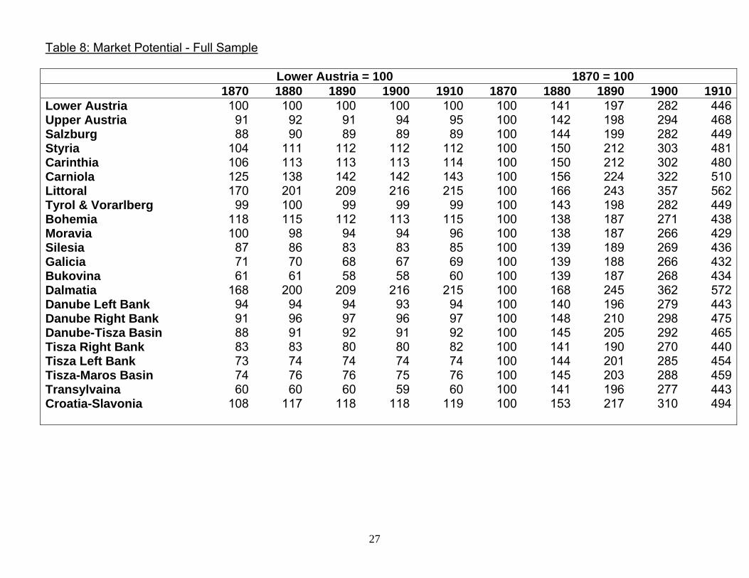
Table 8: Market Potential - Full Sample Lower Austria = 100 1870 = 100 1870 1880 1890 1900 1910 1870 1880 1890 1900 1910 Lower Austria 100 100 100 100 100 100 141 197 282 446Upper Austria 91 92 91 94 95 100 142 198 294 468Salzburg 88 90 89 89 89 100 144 199 282 449Styria 104 111 112 112 112 100 150 212 303 481Carinthia 106 113 113 113 114 100 150 212 302 480Carniola 125 138 142 142 143 100 156 224 322 510Littoral 170 201 209 216 215 100 166 243 357 562Tyrol & Vorarlberg 99 100 99 99 99 100 143 198 282 449Bohemia 118 115 112 113 115 100 138 187 271 438Moravia 100 98 94 94 96 100 138 187 266 429Silesia 87 86 83 83 85 100 139 189 269 436Galicia 71 70 68 67 69 100 139 188 266 432Bukovina 61 61 58 58 60 100 139 187 268 434Dalmatia 168 200 209 216 215 100 168 245 362 572Danube Left Bank 94 94 94 93 94 100 140 196 279 443Danube Right Bank 91 96 97 96 97 100 148 210 298 475Danube-Tisza Basin 88 91 92 91 92 100 145 205 292 465Tisza Right Bank 83 83 80 80 82 100 141 190 270 440Tisza Left Bank 73 74 74 74 74 100 144 201 285 454Tisza-Maros Basin 74 76 76 75 76 100 145 203 288 459Transylvaina 60 60 60 59 60 100 141 196 277 443Croatia-Slavonia 108 117 118 118 119 100 153 217 310 494
27
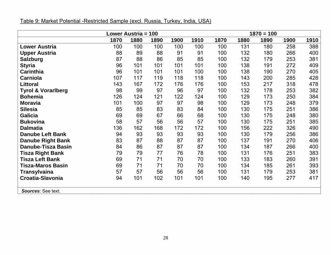
Table 9: Market Potential -Restricted Sample (excl. Russia, Turkey, India, USA) Lower Austria = 100 1870 = 100 1870 1880 1890 1900 1910 1870 1880 1890 1900 1910 Lower Austria 100 100 100 100 100 100 131 180 258 388Upper Austria 88 89 88 91 91 100 132 180 266 400Salzburg 87 88 86 85 85 100 132 179 253 381Styria 96 101 101 101 101 100 138 191 272 409Carinthia 96 101 101 101 100 100 138 190 270 405Carniola 107 117 119 118 118 100 143 200 285 428Littoral 143 167 172 176 176 100 153 217 318 478Tyrol & Vorarlberg 98 99 97 96 97 100 132 178 253 382Bohemia 126 124 121 122 124 100 129 173 250 384Moravia 101 100 97 97 98 100 129 173 248 379Silesia 85 85 83 83 84 100 130 175 251 386Galicia 69 69 67 66 68 100 130 175 248 380Bukovina 58 57 56 56 57 100 130 175 251 385Dalmatia 136 162 168 172 172 100 156 222 326 490Danube Left Bank 94 93 93 93 93 100 130 179 256 386Danube Right Bank 83 87 88 87 87 100 137 191 270 406Danube-Tisza Basin 84 86 87 87 87 100 134 187 266 400Tisza Right Bank 79 79 77 76 78 100 131 176 251 383Tisza Left Bank 69 71 71 70 70 100 133 183 260 391Tisza-Maros Basin 69 71 71 70 70 100 134 185 261 393Transylvaina 57 57 56 56 56 100 131 179 253 381Croatia-Slavonia 94 101 102 101 101 100 140 195 277 417 Sources: See text.
28

Table 10: Market Potential - Considering Habsburg Regions Only Lower Austria = 100 1870 = 100 1870 1880 1890 1900 1910 1870 1880 1890 1900 1910 Lower Austria 100 100 100 100 100 100 124 204 293 383Upper Austria 71 70 69 69 68 100 123 199 283 369Salzburg 56 55 54 53 53 100 123 197 278 365Styria 67 67 67 66 66 100 125 202 290 378Carinthia 53 53 52 51 52 100 124 200 284 373Carniola 52 52 51 50 51 100 124 202 285 377Littoral 44 44 43 42 44 100 124 200 282 381Tyrol & Vorarlberg 48 47 45 44 45 100 122 192 273 362Bohemia 90 89 87 84 85 100 124 198 276 365Moravia 85 84 83 82 83 100 123 199 283 371Silesia 62 62 62 60 61 100 124 203 285 378Galicia 55 56 57 53 54 100 125 211 281 377Bukovina 35 405 35 36 36 37 100 124 212 303Dalmatia 31 32 34 32 33 100 127 221 297 402Danube Left Bank 88 88 88 88 88 100 124 205 292 383Danube Right Bank 60 61 65 63 64 100 125 219 307 404Danube-Tisza Basin 72 74 78 78 80 100 127 219 316 421Tisza Right Bank 55 55 56 55 55 100 123 208 291 384Tisza Left Bank 56 56 58 57 58 100 123 211 297 394Tisza-Maros Basin 53 53 55 53 53 100 124 210 294 387Transylvaina 40 40 40 39 39 100 123 204 283 376Croatia-Slavonia 56 57 57 55 56 100 126 208 291 386 Sources: See text.
29

Map 1: Regions of the Habsburg Empire
30

LONDON SCHOOL OF ECONOMICS ECONOMIC HISTORY DEPARTMENT WORKING PAPERS (from 2003 onwards) For a full list of titles visit our webpage at http://www.lse.ac.uk/ 2003 WP70 The Decline and Fall of the European Film Industry: Sunk Costs,
Market Size and Market Structure, 1890-1927 Gerben Bakker
WP71 The globalisation of codfish and wool: Spanish-English-North
American triangular trade in the early modern period Regina Grafe
WP72 Piece rates and learning: understanding work and production in
the New England textile industry a century ago Timothy Leunig
WP73 Workers and ‘Subalterns’. A comparative study of labour in
Africa, Asia and Latin America Colin M. Lewis (editor)
WP74 Was the Bundesbank’s credibility undermined during the
process of German reunification? Matthias Morys
WP75 Steam as a General Purpose Technology: A Growth Accounting
Perspective Nicholas F. R. Crafts
WP76 Fact or Fiction? Re-examination of Chinese Premodern
Population Statistics Kent G. Deng
WP77 Autarkic Policy and Efficiency in Spanish Industrial Sector. An
Estimation of the Domestic Resource Cost in 1958. Elena Martínez Ruiz
WP78 The Post-War Rise of World Trade: Does the Bretton Woods
System Deserve Credit? Andrew G. Terborgh

WP79 Quantifying the Contribution of Technological Change to Economic Growth in Different Eras: A Review of the Evidence Nicholas F. R. Crafts
WP80 Bureau Competition and Economic Policies in Nazi Germany,
1933-39 Oliver Volckart
2004
WP81 At the origins of increased productivity growth in services.
Productivity, social savings and the consumer surplus of the film industry, 1900-1938 Gerben Bakker
WP82 The Effects of the 1925 Portuguese Bank Note Crisis Henry Wigan WP83 Trade, Convergence and Globalisation: the dynamics of change
in the international income distribution, 1950-1998 Philip Epstein, Peter Howlett & Max-Stephan Schulze WP84 Reconstructing the Industrial Revolution: Analyses, Perceptions
and Conceptions of Britain’s Precocious Transition to Europe’s First Industrial Society
Giorgio Riello & Patrick K. O’Brien WP85 The Canton of Berne as an Investor on the London Capital
Market in the 18th Century Stefan Altorfer WP86 News from London: Greek Government Bonds on the London
Stock Exchange, 1914-1929 Olga Christodoulaki & Jeremy Penzer WP87 The World Economy in the 1990s: A Long Run Perspective Nicholas F.R. Crafts

2005 WP88 Labour Market Adjustment to Economic Downturns in the
Catalan textile industry, 1880-1910. Did Employers Breach Implicit Contracts?
Jordi Domenech WP89 Business Culture and Entrepreneurship in the Ionian Islands
under British Rule, 1815-1864 Sakis Gekas WP90 Ottoman State Finance: A Study of Fiscal Deficits and Internal
Debt in 1859-63 Keiko Kiyotaki WP91 Fiscal and Financial Preconditions for the Rise of British Naval
Hegemony 1485-1815 Patrick Karl O’Brien WP92 An Estimate of Imperial Austria’s Gross Domestic Fixed Capital
Stock, 1870-1913: Methods, Sources and Results Max-Stephan Schulze 2006 WP93 Harbingers of Dissolution? Grain Prices, Borders and
Nationalism in the Hapsburg Economy before the First World War
Max-Stephan Schulze and Nikolaus Wolf WP94 Rodney Hilton, Marxism and the Transition from Feudalism to
Capitalism S. R. Epstein Forthcoming in C. Dyer, P. Cross, C. Wickham (eds.)
Rodney Hilton’s Middle Ages, 400-1600 Cambridge UP 2007 WP95 Mercantilist Institutions for the Pursuit of Power with Profit. The
Management of Britain’s National Debt, 1756-1815 Patrick Karl O’Brien WP96 Gresham on Horseback: The Monetary Roots of Spanish
American Political Fragmentation in the Nineteenth Century Maria Alejandra Irigoin

2007 WP97 An Historical Analysis of the Expansion of Compulsory Schooling
in Europe after the Second World War Martina Viarengo WP98 Universal Banking Failure? An Analysis of the Contrasting
Responses of the Amsterdamsche Bank and the Rotterdamsche Bankvereeniging to the Dutch Financial Crisis of the 1920s
Christopher Louis Colvin WP99 The Triumph and Denouement of the British Fiscal State: Taxation
for the Wars against Revolutionary and Napoleonic France, 1793-1815.
Patrick Karl O’Brien WP100 Origins of Catch-up Failure: Comparative Productivity Growth in
the Hapsburg Empire, 1870-1910 Max-Stephan Schulze WP101 Was Dick Whittington Taller Than Those He Left Behind?
Anthropometric Measures, Migration and the Quality of life in Early Nineteenth Century London
Jane Humphries and Tim Leunig WP102 The Evolution of Entertainment Consumption and the Emergence
of Cinema, 1890-1940 Gerben Bakker WP103 Is Social Capital Persistent? Comparative Measurement in the
Nineteenth and Twentieth Centuries Marta Felis Rota WP104 Structural Change and the Growth Contribution of Services: How
Motion Pictures Industrialized US Spectator Entertainment Gerben Bakker WP105 The Jesuits as Knowledge Brokers Between Europe and China
(1582-1773): Shaping European Views of the Middle Kingdom Ashley E. Millar WP106 Regional Income Dispersion and Market Potential in the Late
Nineteenth Century Habsburg Empire Max-Stephan Schulze