Regional Economies of Scale in Transportation and Regional Welfare

Alexandre Skiba

Department of Economics The University of Kansas

415 Snow Hall Lawrence KS 66045

785 864 2847 skiba@ku.edu

http://www.people.ku.edu/~skiba/research

September 12, 2007

Abstract: A discriminatory tariff can be welfare superior to free trade in the presence of regional economies of scale. This is because a tariff on non-regional trade concentrates trade within a region, lowering the cost of transportation, so that the gains from economies of scale can theoretically offset the losses from the tariff. To complement the theoretical point I estimate the relation between transportation cost and regional volume of trade. The estimates suggest that a 10% increase in the volume of trade brings about 2.5% reduction in transportation cost in the long run.

Keywords: regional economies of scale, transportation costs, preferential trade agreements, regional welfare JEL Classifications: F10, F12

Acknowledgments: The author is grateful to David Hummels for the gracious provision of the data. The paper benefited from helpful suggestions of David Hummels, Russell Hillberry, Volodymyr Lugovskyy, and Jack Barron.

1. Introduction The importance of increasing returns to scale in shipping has long been a focus of

transportation economics. Trade models have begun to focus more intently on the

inclusion of frictions, yet they typically ignore scale effects. This paper studies one

channel through which increasing returns in the transportation industry affect predictions

of trade theory. Particularly, concentration of trade flows as a result of a trade policy can

cause welfare gains from lower transportation costs. In fact, introducing a preferential

tariff may lead to welfare outcomes that are preferred to worldwide free trade.1 The

estimates provided in the empirical section suggest that, holding other things constant, a

10% increase in the regional volume of shipping reduces transportation cost by about

2.5% in the long run and by about 0.6% in the short run. These estimates are valuable for

welfare assessment of trade facilitating practices because regional economies of scale

highlight an important connection between volumes of trade and transportation. This

point is relevant for the policy debate since transport facilitation is an integral part of

trade facilitation efforts in the post Doha negotiations.

The discussion here is closely related to the literature on the welfare consequences

of regionalization,2 which re-entered the academic agenda after the recent wave of

preferential trade agreements registered under the WTO. The main contribution of this

paper to the literature lies in pointing out the importance of the endogenous response of

transportation cost to the changes in trade volumes. This emphasis is motivated by

illustrating how economies of scale can change welfare rankings of different world

1 Previous work includes: Cukrowski and Fisher (2000), who showed how scale economies in transport can reverse Ricardian predictions even if the countries are otherwise identical; and Casas and Choi (1990), who showed that variable returns have implications for economic growth. 2 The extensive literature on preferential trade agreements is summarized in Bhagwati and Panagariya (1996)

1

arrangements and by providing economically significant estimates of regional economies

of scale in transportation.

Recent research on regionalization draws attention to the significance of

transportation costs for welfare consequences of preferential trade agreements.

Spilimbergo and Stein’s (1998) framework often serves as a useful starting point to

account for the cost of transportation. In their model, trade is generated by different

endowments, love for variety, and increasing returns in production. Using this framework

Frankel, Stein, and Wei (1998) show how transportation costs figure in welfare rankings

of preferential trade agreements. The paper most closely related to the present discussion

is Carrere (2005), who introduces a variety of internal scale economies exploited by

monopoly shippers into a setup similar to Spilimbergo and Stein’s. This paper

complements Carrere’s contribution by deriving welfare results analytically and

providing economically meaningful estimates of regional economies of scale. Analytical

tractability is achieved by the choice of utility function and assumption of external

economies of scale. This assumption provides an additional benefit for the empirical

implementation. External economies flexibly encompass a range of technology and

competition related conditions in the transportation industry. The flexibility is empirically

relevant because extremely few routes are served by a single shipper and the exact nature

of competition is often unknown.

This paper differs from prior literature in two ways. First, the implicit assumption

in the regional trade literature is that eliminating tariffs on partners would yield an even

better outcome. This paper asks a stronger question. Can free trade equilibrium be

improved by increasing a tariff on the countries outside the preferential trade area?

2

Second, the model assumes away a production response in order to isolate the

consumption welfare effects. This situation is particularly favorable to free trade because

the consumption effect from a tariff is always negative. In the most general sense, when

consumers make unrestricted choices, i.e. without the tariff distortion, they are able to

achieve a higher utility. In addition, a model with Cobb-Douglas utility and Armington-

differentiated goods, as in Armington (1969), creates a further bias in favor of worldwide

free trade as noted by Deardorff and Stern (1994). Specifically, it is the assumptions of

the uniqueness of each country’s good and perfectly inelastic supply that lead to

maximum welfare loss from the tariff. Allowing for the possibility that a country from

the same bloc can produce a substitute to the goods from outside will lower welfare

losses from creating the blocs.

In the model, countries can either trade freely or be arranged into symmetric

regional trading blocs by raising tariff on outsiders. This preferential tariff raises the

relative price of trade with countries outside the bloc, and concentrates trade flows within

the region. Two competing effects arise. First, lowering trade with countries outside the

bloc leads to a welfare loss because the tariff distorts prices forcing the consumers to buy

inefficiently greater quantities of regional goods. Second, concentrating trade within the

bloc may trigger the use of better shipping technology, thus lowering costs and improving

welfare. For some parameter values, the second effect can dominate. That is, if regional

economies of scale in transport are strong enough, then it is possible to improve world

welfare relative to free trade by forming preferential trading blocs. In this model, free

trade can be problematic because trade is spread too thinly among all partners and the

improved shipping technology is never adopted. The central assumption that drives this

3

result is that transportation costs exhibit regional external economies of scale. Because

the economies of scale are external, a tariff is a way to coordinate price taking consumers

and producers into concentrating trade and exploiting those economies. Since the

economies are regional in scope, no country can unilaterally internalize them.

The empirical section of this paper assesses the economic importance of regional

economies of scale in transportation. The central issue in the estimation of the effect of

trade volumes on freight rates is that causality also runs in the opposite direction: trade

costs impede trade. This is universally supported by the literature on gravity equations,

which suggests that country size variables along with trade costs are important

determinants of cross-country variation in trade volumes. Based on this insight I use

GDP and population to control for variation in quantities of trade that is not due to trade

frictions. The data for this exercise combine information on routes with detailed data on

freight rates and trade volumes. The results of the estimation point to the existence of

economies of scale at the regional level. Moreover, comparison of their estimated

magnitudes to the theoretical model suggests that the regional economies are strong

enough to potentially cause welfare improvement.

2. Sources of regional economies of scale in transportation

The empirical relevance of the model turns on whether there exist regional scale

economies in shipping, and whether they are sufficiently large. Hummels and Skiba

(2004) suggest several sources of transportation cost savings associated with increased

trade volumes. First, containerization of cargo offers tremendous savings on shipping and

handling costs. However, containers are used to different extents on trade routes across

4

the world, with the busiest trading routes having the highest levels of containerization.

Increased containerization occurs on routes with larger volumes because switching to

extensive use of containers on a route requires a fixed cost to adjust or build

infrastructure. Therefore, containerization is feasible only when the volumes of trade are

sufficiently large. Second, significant cost savings can be achieved by using ships that

are specialized or of larger capacity. Large ships significantly lower the unit cost of

shipping, but because of the size, their use is not feasible on low volume routes where

they are replaced by smaller regional feeder-ships. Both sources of economies require an

incremental investment and are more likely to be used for large shipping volumes.3

Third, transit time is reduced when trade rises4. A shipper can expedite delivery in a

number of ways. It can increase the frequency of voyages, reduce the number of port

calls, and/or use routes that are more direct. All of these measures require significant

upfront lump-sum investments and therefore are economically justified only for hig

throughput v

h

olumes.

All of the above mentioned sources of economies inevitably have regional

spillover effects. First, the capacity of modern liners is large relative to the trade volumes

in a given period. Thus, one country may not be able to use large ships up to their

efficient capacity, but a number of countries in a region may provide sufficient volumes

to justify the use of better ships. Second, when two countries establish a major trading

route, the countries along the routes as well as neighboring countries will have access to

more efficient modes of transportation. In other words, had Cote-d’Ivoire been closer to

a large port, say, Rotterdam, the freight rates to the US would have been lower despite

3 Stopford (2002) provides calculations of per unit freight cost for ships of different sizes. 4 See Hummels (2001) for the discussion of cost associated with the duration of the shipping and for an estimation of the implicit ad valorem equivalent of the cost of time

5

greater distance from Rotterdam to the US. Third, the configuration of transportation

networks reflects geographic concentration of trade volumes. A set of countries is more

likely to host a hub or to become a part of a trunk route if their aggregate volume of trade

is large. Mori and Nishikimi (2002) explicitly model endogenous formation of transport

networks to take advantage of scale efficiencies.

3. The Model

The particular choice of trade model is motivated by the question in hand. Firstly,

the model needs to generate trade flows that can be used to investigate the interaction

between volume of trade and per unit transportation cost. Moreover, given that the

question implies a possibility of improvement over free trade, the model is particularly

favorable to worldwide unrestricted trade. Among models that generate volumes of trade

with trade frictions, I choose a combination of Armington differentiation and Cobb-

Douglas preferences over a more general CES (constant elasticity of substitution)

functional form because Cobb-Douglas offers a distinct analytical advantage. CES allows

the expenditure shares to vary with delivered prices and thus trade barriers, while Cobb-

Douglas keeps the shares constant. This invariance of expenditure shares enables the

analytical solution.

The world consists of countries indexed with subscript i: N , 1..i i N∈ =N ,

where N is the set of all countries. Every country i belongs to a region . Country i’s

region is a subset of all countries, , that contains country i, . Each of

iR

iR i ⊂R N ii∈R iL

6

co ntries nsumers in country i maximizes utility from consuming goods k coming from cou

j:

(ln ln , 0,1j

ji ijk

j k

U qθβθ

θ∈ ∈

⎛ ⎞= ⎜ ⎟⎜ ⎟

⎝ ⎠∑ ∑N K

)∈ (1)

subject to a budget constraint:

j

ijk ijk ij k

p q Y∈ ∈

≤∑ ∑N K

(2)

where is income. The expenditure share allocated to goods from country j is equal to

the country’s share in the world income

iY

ij

W

YYβ = and 1j

jβ

∈

=∑N

. The set of goods

produced in country j is denoted by jK . In country i, the price of good k from country j

is , the quantity is . Every good is produced from the inelastically supplied labor

by price taking producers, and every consumer owns the amount of labor required to

produce one unit of the good.

ijkp ijkq

Trade can be impeded by transportation cost and a tariff. In both cases a part of

the delivered good is used in transaction. In the case of transportation cost, a part of the

delivered good “melts” under way. In the case of tariff, the amount of tariff is collected

as percentage of the transaction value and returned to the consumers as a lump sum. The

delivered price can be expressed as a function of domestic, or f.o.b.,5 price of the good k

in country j, jkp , ad valorem equivalent of transportation cost between countries i and j,

1ijφ > , and ad valorem tariff on goods from country j, 1ijτ > :

ijk jk ij ijp p φ τ= (3)

5 “free on board”, an INCOTERMS term commonly used to distinguish the origin price from the delivered price, often denoted as c.i.f., “cost insurance freight”.

7

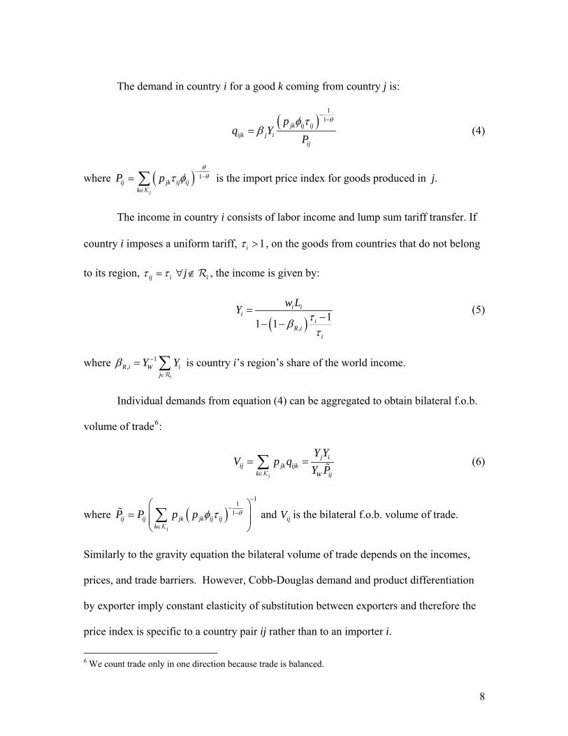
The demand in country i for a good k coming from country j is:

( )

11

jk ij ijijk j i

ij

pq Y

P

θφ τβ

−−

= (4)

where ( ) 1

j

ij jk ij ijk

P pθθτ φ

−−

∈

= ∑K

is the import price index for goods produced in j.

The income in country i consists of labor income and lump sum tariff transfer. If

country i imposes a uniform tariff, 1iτ > , on the goods from countries that do not belong

to its region, ij i ijτ τ= ∀ ∉R , the income is given by:

( ),

11 1

i ii

iR i

i

w LY τβτ

=−

− − (5)

where is country i’s region’s share of the world income. 1,

i

R i W ij

Yβ −

∈

= ∑R

Y

Individual demands from equation (4) can be aggregated to obtain bilateral f.o.b.

volume of trade6:

j

j iij jk ijk

k W ij

Y YV p q

Y P∈

= =∑K

(6)

where ( )1

11

j

ij ij jk jk ij ijk

P P p p θφ τ−

−−

∈

⎛ ⎞= ⎜ ⎟⎟⎜

⎝ ⎠∑K

ij

and V is the bilateral f.o.b. volume of trade.

Similarly to the gravity equation the bilateral volume of trade depends on the incomes,

prices, and trade barriers. However, Cobb-Douglas demand and product differentiation

by exporter imply constant elasticity of substitution between exporters and therefore the

price index is specific to a country pair ij rather than to an importer i.

6 We count trade only in one direction because trade is balanced.

8

Summing up bilateral volumes with exception of domestic purchases yields

regional volume of trade, : ,R iV

(7) ,i i

R i lj lll j

V V∈ ∈

⎛ ⎞= −⎜

⎝ ⎠∑ ∑R R

V ⎟

It is illustrative to rewrite the regional volume as a weighted sum of exporters’ total

volumes of trade:

,i i

lj llR i l

l j l l

V VV VV V∈ ∈

⎛ ⎞= ⎜

⎝ ⎠∑ ∑R R

− ⎟ (8)

where is country l's volume of trade. The weighting term in brackets reflects country

l’s participation in the trade of the i’s region. For example, if country l does not trade

with any other country j from i’s region ,

lV

iR 0 lj iV j= ∀ ∈R , then the weight is zero.

Similar intuition carries over once we express regional volume of trade as a function of

incomes:

,i i

jR i l l

l j lj

V YPβ

β∈ ∈

⎛ ⎞= ⎜⎜

⎝ ⎠∑ ∑R R

− ⎟⎟ (9)

so that the regional volume of trade is a function of the weighted sum of the regional

incomes. As in the case of volumes, the weight reflects country l’s participation in

country i’s regional trade. Based on this insight I later construct the measures of regional

income and regional volume of trade.

Endogenous transportation is the key point of this paper. The traditional iceberg

assumption is relaxed to allow transportation within a region to exhibit external

economies of scale. The final good is still consumed during the delivery but the amount

used up depends on the quantity shipped. While consumers respond to shifts in delivered

9

price given by ijkφ , the shippers are motivated by revenues from delivering a unit of the

good, denoted by ijkf . The two are obviously connected as ( ) /ijk jk ijk jkp f pφ = + . In the

most general case, transportation cost depends on a vector of cost parameters, , such

as distance, weight-to-value ratio, stowage, special handling requirements, and on the

vector of trade volumes, :

ijkX

ijkV

( ),ijk ijk ijkf f= X V (10)

In the empirical specification, I control for a variety of the cost and volume components

but for now consider a parsimonious version of equation (10) sufficient for the theoretical

experiment. Mori and Nishikimi (2002) propose a useful model to relate bilateral unitary

transportation cost, ijf , to the aggregate quantity of shipping in the country i’s region,

, and to the distance between i and j, : ,R iQ ijd

( ),

,

,,

if , ,

if

j ij R i

ij ij R i iijj R i

R i

Fp d c Q cf d Q jd F Fp Q cQ

⎧ <⎪⎪= ⎨

≥⎪⎪⎩

R∀ ∈ (11)

where c and F are cost parameters expressed in units of delivered good. The parameter F

can be thought of as a fixed cost investment that lowers the variable cost by c. Figure 1

shows the cost profile. Economies of scale become effective after regional quantity

surpasses the scale threshold Fc . For countries outside i's region transportation cost is

the value of the “melted” goods:

( ) , ij ij j ij if d p d c j= ∀ R∉ .

10

( ),ij ij Rf d Q

p

On top of its analytical simplicity this model of transportation costs avoids an

additional equilibrium where regional trade is zero and transportation cost is infinite.

Laussel and Riezman (2006) consider such an equilibrium in a model with fixed cost of

transportation.

Next I investigate welfare changes from regional concentration of trade achieved

by a discriminatory non-regional tariff. The following set of symmetry assumptions

significantly simplifies the analysis. All countries are equidistant, ,ijd d i j= ∀ . Each

country produces the same number of goods, K. In the symmetric case there is no reason

for the wages to differ and the trade is automatically balanced. For convenience I

normalize wages to unity: 1 iw i= ∀ ∈N , which fixes prices at 1 ,jkp j k= ∀ . With

prices fixed at unity the volumes of trade equal quantities of trade. The world consists of

R regions, 1R ≥ , each region consists of NR

countries, each country belongs to exactly

RQ Fc

j ijd c

0

Figure 1. Unitary transportation cost with regional external economies of scale

11

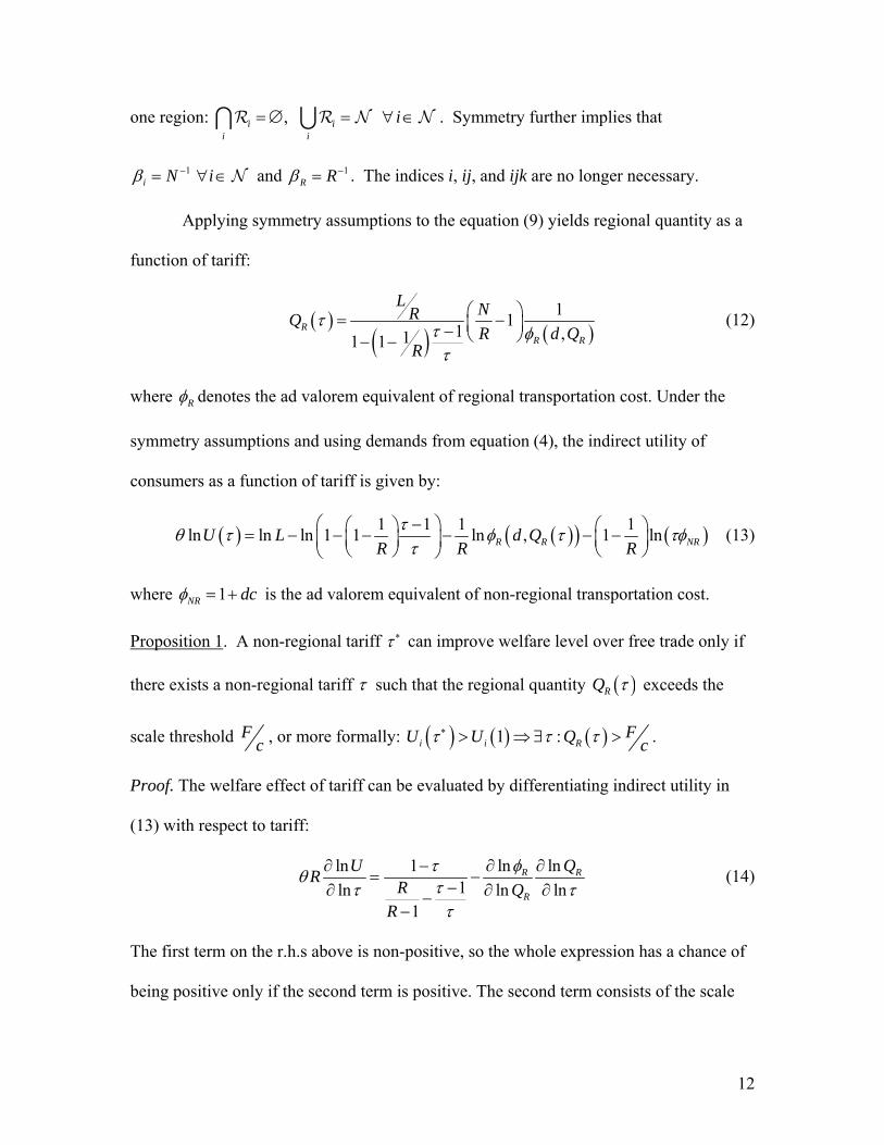
one region: . Symmetry further implies that

and

, i ii i

i=∅ = ∀ ∈∩ ∪R R N N

1 i N iβ −= ∀ ∈N 1R Rβ −= . The indices i, ij, and ijk are no longer necessary.

Applying symmetry assumptions to the equation (9) yields regional quantity as a

function of tariff:

( )( ) ( )

111 ,11 1R

R R

L NRQR d Q

R

τ τ φτ

⎛ ⎞= −⎜ ⎟− ⎝ ⎠− − (12)

where Rφ denotes the ad valorem equivalent of regional transportation cost. Under the

symmetry assumptions and using demands from equation (4), the indirect utility of

consumers as a function of tariff is given by:

( ) ( )( ) (1 1 1 1ln ln ln 1 1 ln , 1 lnR R NU L d QR R R

τ )Rθ τ φ ττ

⎛ − ⎞⎛ ⎞ ⎛ ⎞= − − − − − −⎜ ⎟ ⎜ ⎟⎜ ⎟⎝ ⎠ ⎝ ⎠⎝ ⎠τφ (13)

where 1NR dcφ = + is the ad valorem equivalent of non-regional transportation cost.

Proposition 1. A non-regional tariff τ ∗ can improve welfare level over free trade only if

there exists a non-regional tariff τ such that the regional quantity ( )RQ τ exceeds the

scale threshold Fc , or more formally: ( ) ( ) ( )1 :i i R

FU U Q cτ τ τ∗ > ⇒ ∃ > .

Proof. The welfare effect of tariff can be evaluated by differentiating indirect utility in

(13) with respect to tariff:

ln lnln 11ln ln ln

1

R

R

QUR R QR

Rφτθ ττ ττ

∂ ∂∂ −= −

−∂ ∂−−

∂ (14)

The first term on the r.h.s above is non-positive, so the whole expression has a chance of

being positive only if the second term is positive. The second term consists of the scale

12

elasticity, lnln

R

RQφ∂

∂, and the elasticity of concentration of trade on the regional route. The

elasticity of concentration can be shown to be always positive by differentiating the

regional quantity of trade with respect to tariff.

Substituting the cost of transporting one unit from (11) into equation (12) yields:

( )( )

( )

11 , if 1 111 1

1 , if 111 1

R

R

R

L N FR QR dc c

RQ

L N FR dF QR c

R

τττ

ττ

⎧ ⎛ ⎞⎪ − <⎜ ⎟− +⎪ ⎝ ⎠− −⎪= ⎨⎪ ⎛ ⎞− − ≥⎪ ⎜ ⎟− ⎝ ⎠⎪ − −⎩

Since ( )RQ τ is not globally differentiable, I consider the two cases separately. In both of

them 0RQτ

∂>

∂. The scale elasticity, ln

lnR

RQφ∂

∂, is zero if economies of scale are not

effective and can be negative for some values of τ if and only if the threshold value of

economies of scale, Fc , is smaller than the maximum quantity that can be concentrated

on the regional trade routes, lim RF Qc τ→∞< . It implies that ( ): R

FQ cτ τ∃ > . Q.E.D.

Proposition 1 simply states that economies of scale are a necessary condition for

welfare improvement by a discriminatory tariff. That is, a non-regional tariff cannot

improve welfare unless it induces regional economies of scale. According to Proposition

2 such improvement is also always possible.

Proposition 2. For any values of parameters R, N, L, and d there exists an x such that for

every threshold smaller than x there exists a non-regional tariff τ such that utility level

13

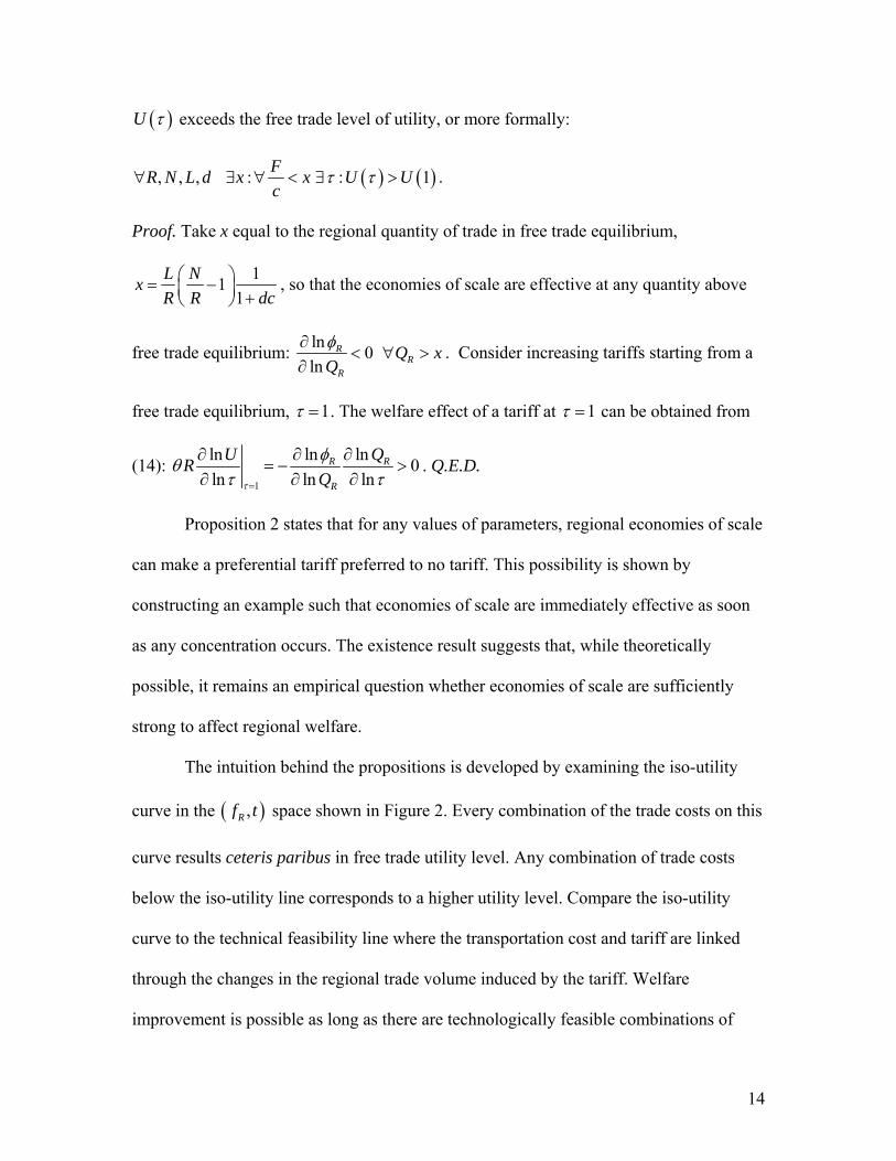
( )U τ exceeds the free trade level of utility, or more formally:

( ) ( ), , , : : 1FR N L d x x U Uc

τ τ∀ ∃ ∀ < ∃ > .

Proof. Take x equal to the regional quantity of trade in free trade equilibrium,

111

L NxR R d⎛ ⎞= −⎜ ⎟ +⎝ ⎠ c

, so that the economies of scale are effective at any quantity above

free trade equilibrium: ln 0 ln

RR

R

QQ

xφ∂< ∀ >

∂. Consider increasing tariffs starting from a

free trade equilibrium, 1τ = . The welfare effect of a tariff at 1τ = can be obtained from

(14): 1

ln lnln 0ln ln ln

R R

R

QURQτ

φθτ τ=

∂ ∂∂= − >

∂ ∂ ∂. Q.E.D.

Proposition 2 states that for any values of parameters, regional economies of scale

can make a preferential tariff preferred to no tariff. This possibility is shown by

constructing an example such that economies of scale are immediately effective as soon

as any concentration occurs. The existence result suggests that, while theoretically

possible, it remains an empirical question whether economies of scale are sufficiently

strong to affect regional welfare.

The intuition behind the propositions is developed by examining the iso-utility

curve in the ( ,R )f t space shown in Figure 2. Every combination of the trade costs on this

curve results ceteris paribus in free trade utility level. Any combination of trade costs

below the iso-utility line corresponds to a higher utility level. Compare the iso-utility

curve to the technical feasibility line where the transportation cost and tariff are linked

through the changes in the regional trade volume induced by the tariff. Welfare

improvement is possible as long as there are technologically feasible combinations of

14

tariffs and transportation costs below the iso-utility curve. The shaded area below the iso-

utility curve and above the line of technological feasibility represents the welfare

improving combinations of non-regional tariffs and regional transportation costs. 9.

89.

69.

410

Reg

iona

l Tra

nspo

rt C

ost,

%9.

2

0 5 10 15Non-Regional Tariff, %

Figure 2. Possibility of welfare improving tariff

Iso-utility curve

Technological feasibility

( Parameter values: 1.21, 10, 1.1, 3, 12.RF L R Nφ= = = = = )

<<<Insert Figure 2 here>>>

The intuition behind Proposition 1 becomes clear by noting that the technological

feasibility line has a negative slope only when the regional economies of scale are

effective. The proof of existence of the welfare improving tariff in Proposition 2 assumes

that the economies of scale are effective immediately starting from the free trade level of

trade. Graphically it would correspond to a situation when the technological feasibility

line starts sloping down from zero tariff.

Before turning to the estimation it is useful to simulate a theoretical benchmark of

scale elasticity which would make a discriminatory tariff on non-regional trade welfare

15

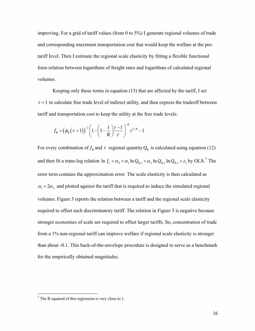
improving. For a grid of tariff values (from 0 to 5%) I generate regional volumes of trade

and corresponding maximum transportation cost that would keep the welfare at the pre-

tariff level. Then I estimate the regional scale elasticity by fitting a flexible functional

form relation between logarithms of freight rates and logarithms of calculated regional

volumes.

Keeping only those terms in equation (13) that are affected by the tariff, I set

1τ = to calculate free trade level of indirect utility, and then express the tradeoff between

tariff and transportation cost to keep the utility at the free trade levels:

( )( ) 1 11 11 1 1R

RR Rf

Rτφ τ ττ

−− −⎛ − ⎞⎛ ⎞= = − −⎜ ⎟⎜ ⎟⎝ ⎠⎝ ⎠

1−

For every combination of Rf and τ regional quantity is calculated using equation RQ (12)

and then fit a trans-log relation 0 1 , 2 , ,ln ln ln lns R s R s R s sf Q Q Qα α α ε= + + +

2

by OLS.7 The

error term contains the approximation error. The scale elasticity is then calculated as

1 2α α+ and plotted against the tariff that is required to induce the simulated regional

volumes. Figure 3 reports the relation between a tariff and the regional scale elasticity

required to offset such discriminatory tariff. The relation in Figure 3 is negative because

stronger economies of scale are required to offset larger tariffs. So, concentration of trade

from a 1% non-regional tariff can improve welfare if regional scale elasticity is stronger

than about -0.1. This back-of-the-envelope procedure is designed to serve as a benchmark

for the empirically obtained magnitudes.

7 The R-squared of this regression is very close to 1.

16

4. Estimation of regional scale economies

This section examines the effect of trade volumes on freight rates. The key to this

exercise is the proper treatment of the endogeneity of freight rates and trade volumes.

While I am interested in the effect of trade volumes on the level of shipping cost, the

inverse effect is present under rather general conditions. Lower trade costs encourage

greater trade. I use tariff and country size variation to trace out exogenous variation in

trade volumes.

-.5-.4

-.3-.2

-.10

Stre

ngth

of R

egio

nal S

cale

Eco

nom

ies

0 1 2 3 4 5Non-Regional Tariff, %

( Pa .rameter values: 1.21, 10, 1.1, 3, 12RF L R N= φ= = = = )

Figure 3. Benchmark strength of regional scale economies.

17

The emphasis on regional trade volumes requires that, along with traditional cost

shifters, I appropriately condition on the other relevant trade volumes: bilateral volume of

trade, , and bilateral quantity of trade in a given commodity, . These volumes of

trade are instrumented by an exporter’s GDP and population, an importer’s GDP and

population, regional GDP and population, and tariffs. The instruments capture theoretical

determinants of volumes given in equation

ijV ijkq

(4) for bilateral quantity of a given

commodity, in equation (6) for total bilateral volume of trade, and in equation (9) for

regional volume of trade.

Special care is devoted to constructing regional volumes of trade. Some obvious

groupings into regions, say by continents, are problematic because in reality every

country often belongs to multiple trading regions. United States’s imports from France

are a part of Europe - North America Atlantic route while imports from China are a part

of the Asia - North America Pacific trade route. The relevant regional volumes of trade

are different despite the same destination. The variable for regional volumes is

constructed to capture actual shipping routes. A country l may frequently but not always

occur on the same itinerary with the exporter j in question. Accordingly, I weight the

country l’s exports to the importer by the frequency with which vessels visiting exporter j

also visit exporter l. The weighted volumes are then summed over all exporters other

than j.

The regional GDP and population are constructed using a similar weighting

scheme to capture the idea of equations (8) and (9) with the data on the actual shipping

routes8. The data on volumes of trade come from NBER UN data set, see Feenstra et al

8 vessel itineraries taken from www.shipguide.com

18

(2005) for a detailed description. GDP’s and populations are taken from PENN world

tables. The volumes of trade are excluded from the subsequent aggregates. The bilateral

volume of a commodity is excluded from the total bilateral volume , and the total

bilateral volume is not included in the regional volume . Data appendix contains

additional detail on the data and provides summary statistics in Tables A1 and A2.

ijkV ijV

,R iV

Long run estimates

Product level import data from five Latin American importers (Argentina, Brazil,

Chile, Paraguay, and Uruguay) and the US in 1994 are used to estimate long run regional

scale elasticities. The data are recorded at 6 digit Harmonized System (HS) commodity

level and include all exporters worldwide. Each observation contains value, weight,

transportation charge, and duty paid. Freight ijkf is calculated as the total shipping

charge divided by total weight of the shipment. Price is calculated as total value of

shipment divided by shipment’s weight. Tariff is calculated in ad valorem terms.

Distance is measured as the greater circle distance between the capitals.

ijkp

ijd

Assume customary log-linear form of the freight rate function in equation (10)

1 2 3 4 5 ,ln ln ln ln ln lnijk k ijk ij ijk ij R i ijkf p d V V Vα β β β β β= + + + + + + ε (15)

Column (2) of Table 1 presents results of IV estimation. The estimated long run

elasticity of freight rates with respect to trade volumes is -.26, implying that a 10% larger

regional volumes of trade correspond to 2.6% lower unitary transportation cost. Column

(3) reports IV estimates of equation (15) with a set of importer dummies. This

specification is a useful robustness check because the US is substantially different from

19

the rest of the importers. However, controlling for importer effect does not substantially

affect the estimates perhaps reflecting the global nature of the shipping industry.

According to the Hausman test, the OLS estimates in column (1) are systematically

different from the IV estimates.

The coefficients on total bilateral volume and volume by commodity in

specifications (2) and (3) are consistent with the idea of lumpy investments in

transportation technology. In order to see this, start by noting that the positive effect of

bilateral trade volume on freight rate does not necessarily imply that there are

diseconomies of scale at bilateral level. A 10% increase in volume of trade of each

commodity for a given country pair increases the aggregate bilateral volume also by 10%.

The resulting effect on shipping rates is still negative and is given by ( )3 4β β+ , -0.73 +

0.49 = -0.24, or a 2.4% reduction in unitary transport cost. Furthermore, a positive 4β

implies that a commodity that is traded in lower volumes than the rest of the commodities

for a given country pair incurs a relatively higher transportation charge. This can be seen

by considering consider a 10% increase in the volume of trade of all commodities traded

between two countries except one commodity k. The average level of transportation cost

is likely to decrease (as long as k is a small share of bilateral volume) but the freight rate

of k will increase because bilateral volume increases. This is consistent with the idea that

once a technology suitable for high volumes is used, shipping smaller volumes becomes

more costly.

Short run estimates

20

Due to the time dimension and greater product detail of the US imports data it is

possible to control for a variety of exporter specific and commodity specific

characteristics and estimate short run response to changes in regional volumes. The US

imports data for 1991-2000 contain the same variables as the Latin American data and are

recorded at 10 digit level of HS classification. The estimating equation is

1 2 3 4 5 ,ln ln ln ln ln lnjkt jk jkt j jkt jt R jt jktf p d V V Vα β β β β β= + + + + + +ε (16)

The results of IV estimation are in column (5) of Table 1. The estimated

magnitude suggests that a 10% increase in regional volume of trade brings about 0.56%

decrease in freight rates. The estimated scale elasticity is smaller than the long run

elasticity consistent with the idea that in the long run the transportation industry can

better exploit differences in regional volumes of trade. The OLS fixed effect estimates in

column (4) are systematically different from the IV estimates according to the Hausman

test.

Economic significance of the estimates

Expressing the estimated magnitudes of scale economies in equivalent distance

savings provides a useful way to appreciate the economic significance of the estimates.

For example, Peru and Morocco are two similar countries that are similarly removed

from the US but have vastly different regional volumes of trade. In 1997 their GDP’s and

total volumes of trade were within 5% of each other’s, and the distance to the US ports is

about the same. The port of Callao, Peru, is about 3900 nautical miles from San

Francisco, while Gibraltar is about 3200 nautical miles to New York. Morocco however

lies on a large number of European trading routes going through Gibraltar. Not

21

surprisingly, the calculated regional volume of trade is 3.7 times higher for Morocco.

According to the estimates, this difference in regional volumes of trade can lead to 3.7.25

≈1.4 times lower shipping rates. In order to achieve such a saving the distance would

have to be reduced 1.41/.345≈2.6 fold. In other words, as a part of a major trading route

Moroccan exporter have to pay 1.4 times less to ship their goods to the US which is

equivalent to 2.6 times shorter distance.

The estimated magnitudes are generally commensurate with the previous findings.

Mori and Nishikimi (2002) survey results from a number of scattered studies that have

looked at the relation between trade quantities and freight rates. Some estimates are

similar to the ones obtained in this paper for a set of Latin American countries and the

US. For example, a 10% increase in the number of ships on a particular route between

Japan and each of the Southeast Asian ports results in a 1.2% reduction in the freight

rates. Table 1 reports similar magnitudes in specifications that do not take into account

endogeneity of trade volumes.

The estimated magnitudes are sufficiently strong to for a discriminatory tariff to

be welfare improving. The theoretical benchmarks in Figure 3 suggest that the estimated

scale elasticity of -.26 is sufficiently strong to offset a small discriminatory tariff on the

order of 2%.

5. Conclusion

Regional scale economies in transportation create a welfare gain when a policy

leads to concentration of trade flows within a region. These economies can theoretically

offset losses from policy distortions. The estimated magnitudes of scale elasticity

22

compare favorably with the benchmark values generated by the model. The positive

implication of this paper is that the effect of regional tariff preference on trade can be

reinforced by regional economies of scale. Regional transportation costs decline

endogenously in response to concentration of trade flows, thus further promoting trade.

The data support this interdependence. Holding other things constant transportation is

cheaper on the busier routes. The normative part of the analysis suggests that the regional

preferential trade agreements create an additional welfare benefit that can make a

regional trading arrangement welfare superior to unrestricted trade. This result arises in a

model where transportation is modeled as a regional positive externality.

The exact nature of the externality requires further investigation because it may

have important policy implications. Some technological changes are irreversible, for

example deepening of a port to allow for larger container ships. In this case, a tariff is

required only as a temporary coordination measure and the concentration will persist

even after the tariff is lifted. On the other hand, the economies could be a result of a

reversible process, such as use of larger ships on heavier routes. This would mean that,

when the tariff is lifted and the price taking consumers switch back to their pre-tariff

behavior, the transportation industry will respond by reverting to less efficient

technology.

In many situations the effect of distance can be more intrusive than presently

modeled. Larger ships tend to be used on the longer routes. This creates a potentially

interesting interaction because economies of scale can be better exploited on the longer

routes.

23

Application of the estimated regional economies to the discussion on

regionalization hinges on a proper definition of a region. Transportation economists and

trade economists might have a different idea of what constitutes a region. For instance,

the US and Japan are a part of the same transportation region, the North Pacific, but they

are rarely put in the same region when discussing costs and benefits of regionalization.

Finally, the discussion in the paper and the empirical results focus explicitly on

transportation costs. However, there are other reasons that unit transaction costs between

two destinations are decreasing in the volume of trade. Some notable examples include

costs of: adapting products to a specific market; establishing communication

infrastructure between two countries; and establishing a distribution network. All of

these can be thought of as technologies that require a fixed cost to reduce the level of

variable cost. Thus, use of a better technology will be justified only by increased

volumes.

24

References Armington P.S., 1969. A theory of demand for products distinguished by place of

production. IMF Staff Papers 16, 159-176. Baum, C.F., Schaffer, M.E., Stillman, S., 2007. ivreg2: Stata module for extended instrumental

variables/2SLS, GMM and AC/HAC, LIML and k-class regression. URL: http://ideas.repec.org/c/boc/bocode/s425401.html

Bhagwati J., Panagariya, A., 1996. The theory of preferential trade agreements: historical

evolution and current Trends. The American Economic Review 86 (2), 82-87. Carrerre, C., 2005. Regional trading agreements and welfare in the south: when scale

economies in transport matter. Etudes et Documents No 2005-13, University of Auvergne.

Casas F. R., Choi, E.K., 1990. Transport innovation and welfare under variable returns to

scale. International Economic Journal 4 (1), 45-57. Cukrowski J., Fisher, F. M., 2000. Theory of comparative advantage: do transportation

costs matter? Journal of Regional Science 40 (2), 311-322. Deardorff, A.V., Stern, R. M., 1994. Multilateral trade negotiations and preferential

trading arrangements, in: A. V. Deardorff and R. M. Stern (eds.), Analytical and Negotiating Issues in the Global Trading System. Ann Arbor, Michigan: The University of Michigan Press.

Feenstra R. C., Lipsey, R.E., Haiyan Deng, Alyson C. Ma, and Hengyong Mo, 2005.

World trade flows: 1962-2000. NBER Working Paper No. 11040. Frankel J.A., Stein, E., and Wei, S., 1998. Continental trading blocks: are they natural or

supernatural? in: J. A. Frankel (ed.), The Regionalization of the World Economy, Chicago: The University of Chicago Press.

Hummels, D., 2001. Time as a trade barrier. Mimeo, Purdue University. Hummels D., Skiba, A., 2004. A virtuous circle? Regional tariff liberalization and scale

economies in transport, in: Antoni Estevadeordal, Dani Rodrik, Alan M. Taylor, Andrés Velasco (eds.), FTAA and Beyond: Prospects for Integration in the America. Harvard University Press.

Laussel, D., Riezman, R., 2006. Fixed transport cost and international trade. Mimeo,

University of Iowa. Mori, T., Nishikimi, K., 2002. Economies of transport density and industrial

agglomeration. Regional Science and Urban Economics 32, 167-200.

25

Spilimbergo, A., Stein, A., 1998. The welfare implications of trading blocs among

countries with different endowments, in: Frankel, J.A., (ed.), The Regionalization of the World Economy. Chicago: University of Chicago Press, 121–45.

Stopford, M., 1999. Maritime Economics. New York: Routledge.

26

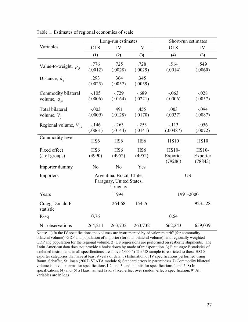
Table 1. Estimates of regional economies of scale

Long-run estimates Short-run estimates OLS IV IV OLS IV

Variables

(1) (2) (3) (4) (5)

Value-to-weight, ijkp .776 (.0012)

.725 (.0028)

.728 (.0029)

.514 (.0014)

.549 (.0060)

Distance, ijd .293 (.0025)

.364 (.0057)

.345 (.0059)

Commodity bilateral volume, ijkq

-.105 (.0006)

-.729 (.0164)

-.689 (.0221)

-.063 (.0006)

-.028 (.0057)

Total bilateral volume, ijV

-.003 (.0009)

.491 (.0128)

.455 (.0170)

.003 (.0037)

-.094 (.0087)

Regional volume, ,R iV -.146 (.0061)

-.263 (.0144)

-.253 (.0141)

-.113 (.00487)

-.056 (.0072)

Commodity level HS6 HS6 HS6 HS10 HS10

Fixed effect (# of groups)

HS6 (4990)

HS6 (4952)

HS6 (4952)

HS10-Exporter (79286)

HS10-Exporter (78843)

Importer dummy No No Yes

Importers Argentina, Brazil, Chile, Paraguay, United States,

Uruguay

US

Years 1994 1991-2000

Cragg-Donald F-statistic

264.68 154.76 923.528

R-sq 0.76 0.54

N - observations 264,211 263,732 263,732 662,243 659,039 Notes: 1) In the IV specifications the volumes are instrumented by ad valorem tariff (for commodity bilateral volume); GDP and population of importer (for total bilateral volume); and regionally weighted GDP and population for the regional volume. 2) US regressions are performed on seaborne shipments. The Latin American data does not provide a brake down by mode of transportation. 3) First stage F statistics of excluded instruments in all specifications are above 4,000 4) The US sample is restricted to those HS10-exporter categories that have at least 9 years of data. 5) Estimation of IV specifications performed using Baum, Schaffer, Stillman (2007) STATA module 6) Standard errors in parentheses 7) Commodity bilateral volume is in value terms for specifications 1,2, and 3, and in units for specifications 4 and 5. 8) In specifications (4) and (5) a Hausman test favors fixed effect over random effects specification. 9) All variables are in logs

27

Data Appendix

Imports and Transport Cost Data. US Census Bureau, “US Imports of Merchandise”. These data report extremely detailed customs information on US imports from all exporting countries (approximately 160) for 1991-2000. The data are reported at the 10 digit Harmonized System level (approximately 15300 goods categories). The data is aggregated to the 6 digit level for comparability with the other trade data in the long run specifications. Data include the valuation of imports, inclusive and exclusive of freight and insurance charges, shipment quantity (by count and by weight), transportation mode, district of entry into the US, and duties paid. Goods are valued FAS, or “free alongside ship” meaning that freight charges include loading and unloading expenses. ALADI Secretariat, “Latin American Trade”. Reports imports of Argentina, Brazil, Chile, Paraguay, and Uruguay from 1994 at the 6 digit Harmonized System coding (approximately 3000 goods). Data include exporter, value of imports, weight, freight charges and insurance charges (separately). Freight charges are based on FOB ("free on board" - exclusive of loading costs") valuation of goods. For overland transport within the ALADI countries it appears that the freight field has a zero value. This is because charges are only incurred between exit and entry ports, and these are the same for overland transport. Note, however, that this does not change the relative valuation of freight charges across export partners. All trade incurs some overland shipping from factory to exporting port and from importing port to location of consumption and these costs are missing from all the data. One can then think of the observed values as a distribution that is simply shifted to the left relative to the true set of values. Other Data Tariff Data Bilateral tariff data at the 6 digit HS level are available for the six importers. While the precise year varies somewhat across countries, most of the data are from 1994. The data originally come from the TRAINS dataset, and we employ a special extract provided by Jon Haveman that painstakingly constructed bilateral tariff rates using preference indicators in these data. See Haveman, Nair, and Thursby, 1998a,b. Shipping Schedule

Data on ocean shipping times are derived from a master schedule of shipping for 1999 taken from www.shipguide.com. This shipping schedule describes all departures and arrivals of all commercial vessels operating worldwide in this period. From this, we construct a matrix of shipping times between all ports everywhere in the world and all US entry ports. Several modifications are necessary. First, direct shipments are not available for every port-port combination (Tunis does not ship directly to Houston). In these cases,

28

I calculate all possible combinations of indirect routings (Tunis to Rotterdam to Houston; Tunis to Rio to Houston and so on) and take the minimum shipment time available through these routings. Second, there are generally multiple ports within each origin country. In this section, a within-country average of shipment time from these ports is employed. Because US data include entry port detail, these are combined with destination-port specific arrival times.

29

Table A1. Summary statistics of the variables in the Latin American – US data set. Statistic

Variable Unit value Mean Standard deviation

Ad valorem freight rate 0.13 0.18 Distance Km 9,033 4,836 Exporter's population million 99.9 216.7 Exporter's GDP $, billion 1,130 1,800 Importer's population million 129.8 114.1 Importer's GDP $, billion 3,040 3,510 Route weighted population million 951.8 654.2 Route weighted GDP $,billion 10,200 2,530 Commodity level trade volume $,000 2,483 73,500 Bilateral volume of trade $, billion 7.4 21.0 Route weighted volume of trade $, billion 4,290 1,150

Table A2. Summary statistics of the variables in US data set.

Statistic Variable Unit value

Mean Standard deviation Ad valorem freight rate 0.072 0.086 Exporter's population million 143.9 317.0 Exporter's GDP $, billion 995 1,260 Importer's population million 278.3 11.5 Importer's GDP $, trillion 8.90 1.18 Route weighted population million 1,016 782 Route weighted GDP $,trillion 6.59 2.79 Commodity level trade volume $,000 3,060 56,100 Bilateral volume of trade $, billion 15.5 25.6 Route weighted volume of trade $, billion 2,170 1,870

30