regional climate simulation for korea using dynamic

Journal of the Meteorological Society of Japan, Vol. 82, No. 6, pp. 1629--1643, 2004 1629

Regional Climate Simulation for Korea using Dynamic Downscaling

and Statistical Adjustment

J.-H. OH, T. KIM

Department of Environmental Atmospheric Sciences, Pukyong National University, Busan, Korea

M.-K. KIM

Department of Atmospheric Science, Kongju National University, Chungnam, Korea

S.-H. LEE

Department of Geography, Konkuk University, Seoul, Korea

S.-K. MIN and W.-T. KWON

Meteorological Research Institute, the Korea Meteorological Administration, Seoul, Korea

(Manuscript received 18 June 2003, in final form 18 June 2004)

Abstract

Recently the regional impact assessment due to global warming is one of the urgent tasks to everycountry in the world, under the circumstances of increasing carbon dioxide in the atmosphere. This as-sessment must include not only meteorological factors, such as surface air temperature and precipita-tion, etc., but also the response of the local ecosystem. Based on a previous study, for example, it hasbeen known that Phyllostachys’ habitation, which is one of the bamboo species popular in Korea, is quitesensitive to temperature change, in particular during the winter season. Thus, adequate climate infor-mation is essential to derive a solid conclusion on the regional impact assessment for future climatechange.

In this study, we adopted a dynamical downscaling technique to get regional future climate informa-tion, with the regional climate model (MM5, Pennsylvania State University/National Center for Atmo-spheric Research mesoscale model) from the Max-Planck Institute for Meteorology Models and DataGroup’s Atmosphere-Ocean General Circulation Model (AOGCM) ECAHM4, and HOPE-G (ECHO-G)simulation for future climate, based on future greenhouse gas (GHG) emission scenario of the Inter-governmental Panel on Climate Change (IPCC) Special Report on Emission Scenarios (SRES) A2.Through this nesting process we got reasonable regional climate change information. However, we founda couple of systematic differences, such as a cold bias in the surface air temperature, simulated by MM5compared to that by the AOGCM ECHO-G. This cold bias may cause to loose credibility on the futureclimate scenario to the impact assessment studies. Accordingly, we introduced a transfer function tocorrect the systematic bias of the dynamic model in the regional-scale, and to predict the regional cli-

Corresponding author: Jai-Ho Oh, IntegratedClimate System Modeling Group, Department ofEnvironmental Atmospheric Sciences, PukyongNational University, 599-1 Daeyeon3-dong, Nam-gu, Busan 608-737, South Korea.E-mail: [email protected]( 2004, Meteorological Society of Japan

mate from large-scale predictors. These transfer functions are obtained from the daily mean temperatureof 17 surface observation stations in Korea for 10 years from 1992 to 2001, and 10-year simulation dataobtained from regional climate model (RCM) for each mode of EOFA to correct the systematic bias ofRCM data.

With these transfer functions, we can correct the RMS error of the daily mean temperature in RCMas much as 47.6% in winter and 86.5% in summer. After dynamical downscaling and statistical adjust-ment, we may provide adequate climate change information for regional assessment studies.

1. Introduction

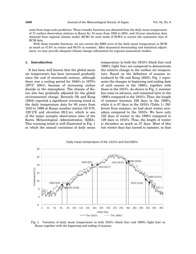
It has been well known that the global meanair temperature has been increased graduallysince the end of nineteenth century, althoughthere was a cooling period for 1940’s to 1970’s(IPCC 2001), because of increasing carbondioxide in the atmosphere. The climate of Ko-rea also has gradually adjusted for the globalenvironmental change. Recently Oh and Kang(2004) reported a significant warming trend inthe daily temperature data for 90 years from1910 to 1999 at Busan weather station (35�6 0N,129�2 0E and elevation 69.2 m), which is oneof the major synoptic observation sites of theKorea Meteorological Administration (KMA).This warming trend is well illustrated in Fig. 1in which the annual variations of daily mean

temperature in both the 1910’s (black line) and1990’s (light line) are compared to demonstratethe relative change in the surface air tempera-ture. Based on the definition of seasons in-troduced by Oh and Kang (2003), Fig. 1 repre-sents the changes in beginning and ending dateof each season in the 1990’s, together withthose in the 1910’s. As shown in Fig. 1, summerhas come in advance, and remained later in the1990’s compared to the 1910’s. Thus, the lengthof summer becomes 109 days in the 1990’s,while it is 87 days in the 1910’s (Table 1). Dif-ferent from summer, we had short winter now-adays compared to the 1910’s. We have only102 days of winter in the 1990’s compared to129 days in 1910’s. Thus, the length of winteris shrunken as much as 27 days. Most of thislost winter days has turned to summer, so that

Daily mean temperatture of the 1910''s and the1990''s

1910 (6/17)

1910 (11/9)

1910 (3/19)

1910 (9/12) 1990 (9/18)

1990 (3/3)

1990 (11/21)

-5

0

5

10

15

20

25

30

Julian Day

Tem

pera

ture

(°C

)

1990 (6/1)

The 1910's The 1990's

1 21 41 61 81 121 161 181 201 221 241 261 281 301101 141 321 341 361

Fig. 1. Variation of daily mean temperature in both 1910’s (black line) and 1990’s (light line) atBusan together with the beginning and ending of seasons.

Journal of the Meteorological Society of Japan1630 Vol. 82, No. 6

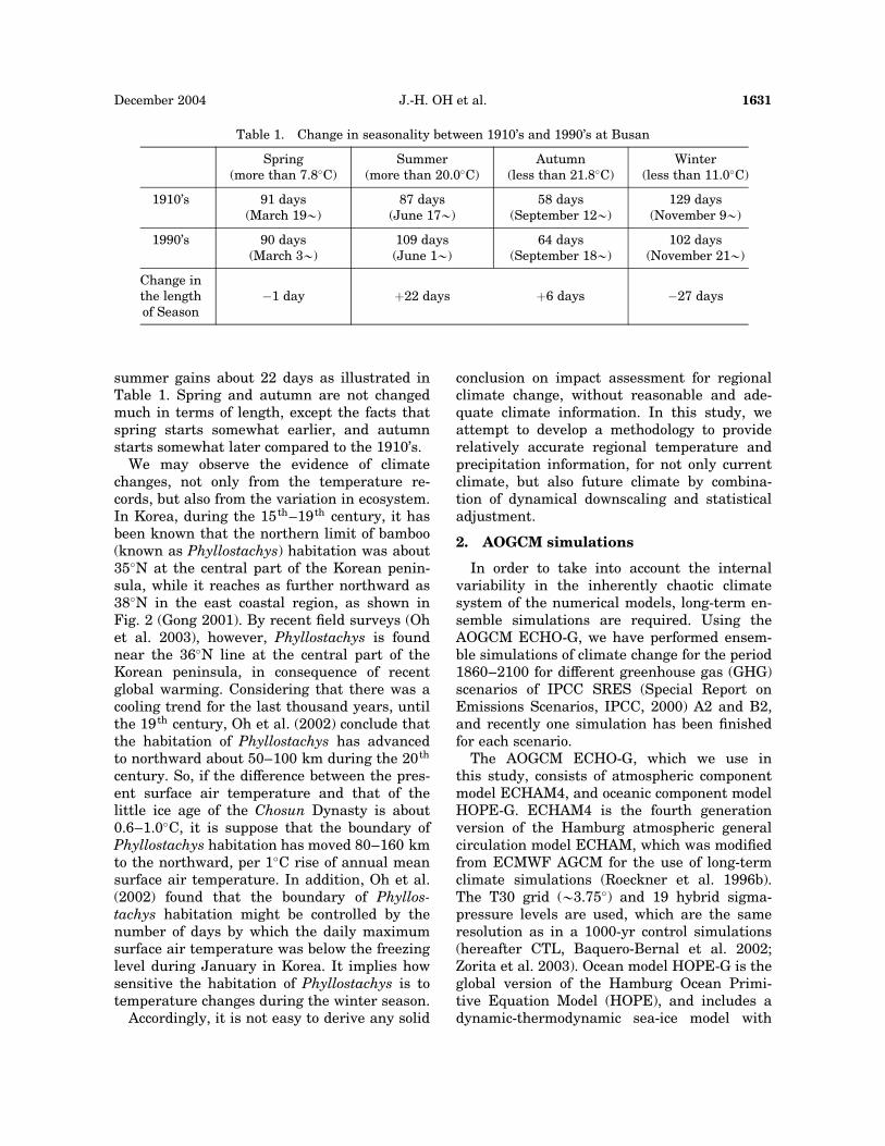
summer gains about 22 days as illustrated inTable 1. Spring and autumn are not changedmuch in terms of length, except the facts thatspring starts somewhat earlier, and autumnstarts somewhat later compared to the 1910’s.

We may observe the evidence of climatechanges, not only from the temperature re-cords, but also from the variation in ecosystem.In Korea, during the 15th–19th century, it hasbeen known that the northern limit of bamboo(known as Phyllostachys) habitation was about35�N at the central part of the Korean penin-sula, while it reaches as further northward as38�N in the east coastal region, as shown inFig. 2 (Gong 2001). By recent field surveys (Ohet al. 2003), however, Phyllostachys is foundnear the 36�N line at the central part of theKorean peninsula, in consequence of recentglobal warming. Considering that there was acooling trend for the last thousand years, untilthe 19th century, Oh et al. (2002) conclude thatthe habitation of Phyllostachys has advancedto northward about 50–100 km during the 20th

century. So, if the difference between the pres-ent surface air temperature and that of thelittle ice age of the Chosun Dynasty is about0.6–1.0�C, it is suppose that the boundary ofPhyllostachys habitation has moved 80–160 kmto the northward, per 1�C rise of annual meansurface air temperature. In addition, Oh et al.(2002) found that the boundary of Phyllos-tachys habitation might be controlled by thenumber of days by which the daily maximumsurface air temperature was below the freezinglevel during January in Korea. It implies howsensitive the habitation of Phyllostachys is totemperature changes during the winter season.

Accordingly, it is not easy to derive any solid

conclusion on impact assessment for regionalclimate change, without reasonable and ade-quate climate information. In this study, weattempt to develop a methodology to providerelatively accurate regional temperature andprecipitation information, for not only currentclimate, but also future climate by combina-tion of dynamical downscaling and statisticaladjustment.

2. AOGCM simulations

In order to take into account the internalvariability in the inherently chaotic climatesystem of the numerical models, long-term en-semble simulations are required. Using theAOGCM ECHO-G, we have performed ensem-ble simulations of climate change for the period1860–2100 for different greenhouse gas (GHG)scenarios of IPCC SRES (Special Report onEmissions Scenarios, IPCC, 2000) A2 and B2,and recently one simulation has been finishedfor each scenario.

The AOGCM ECHO-G, which we use inthis study, consists of atmospheric componentmodel ECHAM4, and oceanic component modelHOPE-G. ECHAM4 is the fourth generationversion of the Hamburg atmospheric generalcirculation model ECHAM, which was modifiedfrom ECMWF AGCM for the use of long-termclimate simulations (Roeckner et al. 1996b).The T30 grid (@3.75�) and 19 hybrid sigma-pressure levels are used, which are the sameresolution as in a 1000-yr control simulations(hereafter CTL, Baquero-Bernal et al. 2002;Zorita et al. 2003). Ocean model HOPE-G is theglobal version of the Hamburg Ocean Primi-tive Equation Model (HOPE), and includes adynamic-thermodynamic sea-ice model with

Table 1. Change in seasonality between 1910’s and 1990’s at Busan

Spring(more than 7.8�C)

Summer(more than 20.0�C)

Autumn(less than 21.8�C)

Winter(less than 11.0�C)

1910’s 91 days(March 19@)

87 days(June 17@)

58 days(September 12@)

129 days(November 9@)

1990’s 90 days(March 3@)

109 days(June 1@)

64 days(September 18@)

102 days(November 21@)

Change inthe lengthof Season

�1 day þ22 days þ6 days �27 days

J.-H. OH et al. 1631December 2004

snow cover. A gaussian T42 grid (about 2.8�) isused, with the meridional refinement of 0.5� inthe tropical band between 10�S and 10�N, andvertical resolution is by 20 horizontal layers.ECHAM4 and HOPE-G exchange 10 atmo-spheric fluxes and 4 ocean and sea-ice informa-tion once in a day. Annual mean heat andfreshwater fluxes, as diagnosed from the relax-ation term during the spin-up, are used as fluxcorrections. However, no momentum flux cor-rections are used. This flux correction methodhas a merit of leaving the seasonal cycle andthe wind stress determined by model physics,and has been used in the ECHAM4/OPYC3whose atmospheric component is the same asthat of ECHO-G, except for the different hori-zontal resolution of T42 gaussian grid (Roeck-ner et al. 1996a, 1999; Bacher et al. 1998;

Stendel et al. 2002). For more details of ECHO-G, see Legutke and Voss (1999).

In climate change simulations with ECHO-G, a total of 19 well-mixed GHGs (greenhousegases) are used including CO2, CH4, N2O, andindustrial halocarbons. GHG concentrationsare constructed from observations for the pe-riod 1860–1990, and SRES A2 or B2 markerscenarios for the period 1990–2100. These sim-ulations include GHGs only referred to as A2Gand B2G, which represent pessimistic and op-timistic scenarios, respectively. In the A2G[B2G] scenario, for example, CO2 concentrationincreases up to@821 [@606] ppm by 2100. A2Gand B2G are initialized at year 311 of CTL.Because, in CTL, present-day observations areused to estimate flux corrections and spin-upthe ocean model and 1990 concentrations ofmain GHGs (CO2, CH4, N2O) are appliedrather than preindustrial ones, there is an ini-tial shift in concentrations of the main GHGsin A2G and B2G. This initial shift is consideredby enhancing both the observed and projectedconcentrations of the main GHGs in an appro-priate way by Roeckner et al. (1999). As such,initial warm bias compared to observations, ismaintained though the whole simulation, sothe derived climate trends are not affected(Roeckner et al. 1999; Stendel et al. 2002).

East Asian (defined as the grid box of80�E@180�E and 20�N@60�N) climate changesin A2G and B2G, are analyzed focusing on thechanges of near surface temperature and pre-cipitation. Analysis results show that East Asiais likely to experience warmer and wetter cli-mate than present, with larger amplitude thanglobal mean (see Fig. 3). The A2G [B2G] [email protected] [4.5]�C increase of temperature [email protected] [6.0]% increase of precipitation over EastAsia by 2100, as seen in the lower panels inFig. 3. However, it should be noted that precip-itation projection has a large uncertainty fromthe dominant interannual and decadal vari-ability, which cannot be reliably estimatedfrom a single realization. Spatial pattern ofclimate change over East Asia shows that thenorthern continental area has larger warmingthan the southern oceanic area, while the pre-cipitation change is dominant over the coastalarea of East Asia (see Fig. 4). Local climatechange over the Korean Peninsula are pro-jected as about 5@7 [3@5]�C and 10@30

Fig. 2. The comparison for distribution ofPhyllostachys between preceding studyand present in Korea. The grey lineis the northern limit of Phyllostachyshabitation during 15–19th century by(Gong 2001) and the dots representfield survey (Oh et al. 2002).


Fig. 3. Time series of annual mean near surface temperature change [�C] (left panels) and precipi-tation change [%] (right panels) for the period of 1860–2100 in ECHO-G A2G (B2G) simulations: a)globe mean and b) East Asia mean. Thick (thin) solid lines show A2G (B2G) results.

Fig. 4. Climate change patterns over East Asia of temperature [�C] (left panels) and precipitation[%] (right panels) for the period of 2070–2099 in ECHO-G a) A2G and b) B2G simulations. Changesare evaluated from the 30-year mean of 1961–1990. Area-averaged values are shown at the righttop of each panel.


[10@20]% increase in A2G [B2G] by 2100, butlarge uncertainty should be taken into account.It is interesting to see that there is seasonaldependencies of climate change over East Asia:surface temperature increases in cold season(SON, DJF) are @0.5�C stronger than in warmseason (MAM, JJA), while precipitation in-crease in summer (JJA) is dominantly largerthan other seasons, which might be related tothe strengthening of East Asian summer mon-soon system (figures not shown). A precise in-vestigation on the seasonal dependency of cli-mate change might be necessary in the future.It is worthy to note that these analysis resultshave a large uncertainty, especially in the pro-jection of precipitation change, because only asingle realization of ECHO-G is used in theanalysis.

3. Dynamic downscaling

Although the resolution of Atmosphere-Ocean General Circulation Models (AOGCMs)is still coarse, simulations of present day cli-mate with the AOGCMs become quite compa-rable to the observed atmospheric generalcirculation features in general since the IPCCWGI Second Assessment Report (IPCC, 1996)(hereafter SAR). Meanwhile, the developmentof high resolution Atmospheric General Circu-lation Models (AGCMs) shows that the models’dynamics and large-scale flow improve as reso-lution increases, though this is not uniformly sogeographically or across models (e.g., Stratton1999; Cubasch et al. 1995; Deque and Piedelie-vre 1995). In some cases, however, systematicerrors are worsened compared with coarserresolution models although only very few re-sults have been documented. The direct useof high-resolution versions of current AGCMs,without some allowance of the dependence ofmodels physical parameterizations on resolu-tion, leads to some deterioration in the per-formance of the models. At the regional scale,in particular, the models display area-averagebiases that are highly variable from region-to-region and among models, with sub-continentalarea-averaged seasonal temperature biasestypically within 4�C, and precipitation biasesmostly between �40 and þ80% of observations(IPCC, 2001).

Regional Climate Models (RCMs) based onthe concept of ‘‘downscaling’’, implying that the

regional climate is conditioned, but not com-pletely determined by the larger scale state,consistently improve the spatial detail of simu-lated climate compared to General CirculationModels (GCMs) since SAR. The conclusionsreported in SAR were that (a) both RCMs anddownscaling techniques showed a promisingperformance in reproducing the regional detailin surface climate characteristics as forced bytopography, lake, coastlines and land use dis-tribution; and (b) high resolution surface forc-ing can modify the climate change signal at thesurface on the sub-AOGCM grid scale. RCMsdriven by observed boundary conditions showarea-averaged temperature biases (regionalscales of 105 to 106 km2), generally within 2�C,and precipitation biases within 50% of observa-tions (IPCC, 2001).

The nested regional modeling technique es-sentially originated from numerical weatherprediction, and Dickinson et al. (1989) andGiorgi (1990) pioneered the use of RCMs forclimate application. RCMs are now used in awide range of climate applications, from pa-laeoclimate to anthropogenic climate changestudies. They can provide high resolution (up to10 to 20 km or less) and multi-decadal simu-lations, and are capable of describing climatefeedback mechanisms acting at the regionalscale. A number of widely used limited areamodeling systems have been adapted to, or de-veloped for, climate application. More recently,RCMs have begun to couple atmosphericmodels with other climate process models, suchas hydrology, ocean, sea-ice, chemistry/aerosoland land-biosphere models.

One of the important issues in long-term in-tegrations using dynamic downscaling methodis nesting of RCMs to coarse large-scale do-main, to prevent long-term drift between thesolutions of the coarse and nested domains.Hong and Juang (1998) demonstrated thatregional model forecasts are consistent withcoarse model forecasts without a discerniblesystematic bias, by introducing a simple orog-raphy blending technique near the lateralboundary of the regional model, with that ofa coarse model. A similar linear orographyblending method has been adopted for long-term integration of RCM. For a regional cli-mate simulation, MM5 (version 3.4) with 27km horizontal resolution, and 18 layers of s-


coordinate in vertical, is nested within the out-put of IPCC SRES A2 experiment, provided bythe AOGCM ECHO-G for the period of modelyear 2001 to 2030 (details are in Oh et al.2002).

In the regional simulations, the MM5 wasdriven by updating the lateral boundary condi-tions at 4-hour intervals using the interpolatedECHO-G data. Its lateral boundary conditions,such as sea level pressure (Pa), the longitudi-nal and latitudinal wind (m/s), specific humid-ity (kg/kg), temperature (K) and geopotentialheight (gpm) as listed in Table 2. Figure 5shows the time series of monthly mean airtemperature for East Asia, simulated by bothAOGCM ECHO-G and MM5 for 30 years from2001 to 2030. The time series of air tempera-

ture simulated by MM5 has followed that ofAOGCM ECHO-G, however, the cold bias hasbeen found in the simulation by MM5 com-pared to AOGCM ECHO-G. This cold bias has atendency to be shrunken during the summerseason and enlarged during the winter season(Fig. 5). Although the nested model has triedto catch up, the initial cold bias through inte-gration is so slow that the bias may remain atleast for a significant period in the 100 yearsintegration. It can be mislead when the MM5output is used in the studies on regional cli-mate change assessment without adequatetreatment. We will discuss this matter in detailat section 4.

The left panels in Fig. 6 show the seasonalmean air temperature in East Asia by the GCM(upper) and RCM (MM5) (lower), respectively.The results of RCM are quite similar to those ofGCM, except regional details mostly come fromdetail topography used in RCM. For summer,(JJA) significant warming in south China inlarge-scale climate data by AOGCM has beenremoved by RCM. In addition, RCM producessurface air temperature at mountainous regionmore realistically than AOGCM. A similar con-clusion can be derived from other seasons. Thecold area in northern Majuria has expendedto further south in RCM compared to AOGCM.These are highly encouraging features for the

Table 2. List of ECHO-G variables usedto the initial and lateral boundary con-ditions for RCM (MM5)

Variable Unit

U-velocity [m/s]V-velocity [m/s]Temperature [K]Specific humidity [kg/kg]Sea level pressure [Pa]Geopotential height [gpm]

Fig. 5. Time series of surface air temperature simulated by both AOGCM and MM5 (upper panel)together with their difference (MM5—AOGCM) (lower panel) for the period from model year 2001to 2030.


studies on the impact assessment for climatechange. We may reach to the same conclusionwith precipitation simulations. Similar to tem-perature changes, the right panels in Fig. 6present the seasonal precipitation changes (%)for the model year 2001 to 2030 by GCM (up-per) and RCM (lower), respectively. For all sea-sons, the development of monsoon is well or-ganized in the RCM simulation compared tothat in GCM. In the right upper panel in Fig. 7,we hardly have to see such an organized mon-soon development, mainly due to its coarsehorizontal resolution. Another distinguishedfeature is that there is less precipitation in thenorthern and eastern part of East Asia. Wecould not find any particular cause for this fea-ture, however, we suspect a boundary problem

in nesting.

4. Statistical adjustment

Transfer function approaches have sub-sequently emerged to satisfy the need to correctthe systematic bias of dynamic model in theregional-scale, or to predict the regional climatefrom large-scale predictors (Kim et al. 1984;Wigley et al. 1990; Wilby et al. 1998; Kim et al.2004). Fundamental to this approach is theassumption that stable empirical relationshipscan be established between atmospheric pro-cesses occurring at disparate temporal and/orspatial scales (Wilby et al. 1998). A major partof this systematic error can be corrected bythe statistical relationship between model dataand observed data, the so-called principal

Fig. 6. Seasonal temperature change [�C] for the model year 2001 to 2030 by both GCM (left panels)and RCM (right panels) for (a) MAM, (b) JJA, (c) SON, and (d) DJF, respectively.

Fig. 7. Seasonal precipitation change [%] for the model year 2001 to 2030 by both GCM (left panels)and RCM (right panels) for (a) MAM, (b) JJA, (c) SON, and (d) DJF, respectively.


component analysis such as coupled patterntechnique, regression analysis and empiricalorthogonal function analysis (EOFA). Mostcommonly used methodologies of the coupledpattern technique are based on singular valuedecomposition analysis (SVDA), and canonicalcorrelation analysis (CCA). Ward and Navarra(1997) applied SVDA to simultaneous fieldsof GCM simulated precipitation and observedprecipitation to correct the errors in model re-sponse to SST forcing. A recent study by Fed-dersen et al. (1999) demonstrated, however,that the post-processed results are not sensi-tive to the choice among the methods basedon the CCA, SVD, and EOFA. In this study,the systematic bias of RCM was corrected bythe transfer function, which is constructed byEOFA and simple linear regression analysis.

a. Methodology of adjustment for systematicbias

The observed data used in this study are thedaily mean temperature of 17 surface observa-tion stations in Korea for 10 years from 1992to 2001, and two 10-year simulation data ob-tained from a regional climate model (RCM),with the period 1992–2001 and 2021–2030.Based on the empirical orthogonal functionanalysis (EOFA), and simple linear regressionanalysis, the transfer functions are obtained foreach mode of EOFA to correct the systematicbias of RCM data.

Let Xðx; tÞ and Yðy; tÞ be RCM data, and theobserved data with time ðtÞ and space (x or y),respectively where xðyÞ are from 1 to pðqÞ. pand q are the number of grid point in RCM andstation in observation, respectively. The repre-sentation of the data are as follows, based onEOFA

Xðx; tÞ ¼XP

i¼1

emi ðxÞT m

i ðtÞ ð1Þ

Yðy; tÞ ¼Xq

i¼1

eoi ðyÞT o

i ðtÞ ð2Þ

where ei and Ti indicate the eigen vector andnormalized time coefficient of each mode, re-spectively. The superscript o and m indicatethe observation and model, respectively.

The first step is to find the main modes withthe similar dynamical origin, such as seasonal

cycle in both sides from EOFA. Then the secondstep is to obtain the relationship between T m

i ðtÞand T o

i ðtÞ for each mode from simple linear re-gression analysis.

TEoi ðtÞ ¼ b0i þ b1iT

mi ðtÞ ð3Þ

where b0i and b1i indicate regression coeffi-cients of each mode i. TEo

i ðtÞ means the esti-mated time coefficients of T o

i ðtÞ. The third stepis to reconstruct the corrected distribution us-ing equation (4).

Cðy; tÞ ¼Xq

i¼1

eoi ðyÞTEo

i ðtÞ ð4Þ

where Cðy; tÞ indicates the corrected valueof RCM data. The final bride to complete thetransfer function is equation (5), which pro-vides the bridge to obtain TEo

i ðtÞ in equation (3)for given Xðx; tÞ.

T mi ðtÞ ¼

Xp

x¼1

Xðx; tÞemi ðxÞ ð5Þ

We named these procedures Empirical Or-thogonal Transfer function (EOTF) method. Ifwe can obtain the transfer function between theobservation and RCM data for the training pe-riod like the control run, the corrected RCMoutput will be able to obtain from RCM datafor the CO2 increasing condition based on theEOFT method. The credibility of this methoddepends on the strong relationship betweenthe observation and Model data in the leadingeigen modes of EOFA.

b. Application to RCM dataIn application, we obtained the leading two

modes from EOFA for daily mean temperaturein Korea. In observation the eigen vector ofthe first mode has the positive sign in all theregions, but larger value toward inland thanalong the coast, indicating that the seasonalcycle has large amplitude inland (Fig. 8a).The first mode shows the seasonal cycle, withstrong positive signal in August and negativesignal in February (Fig. 8b). The second modeshows another seasonal cycle related to theocean effect (Figs. 8c, d). The eigen vector of thesecond mode has the east-west pattern withthe positive value along the coast, and negativevalue toward inland (Fig. 8c). The amplitude of


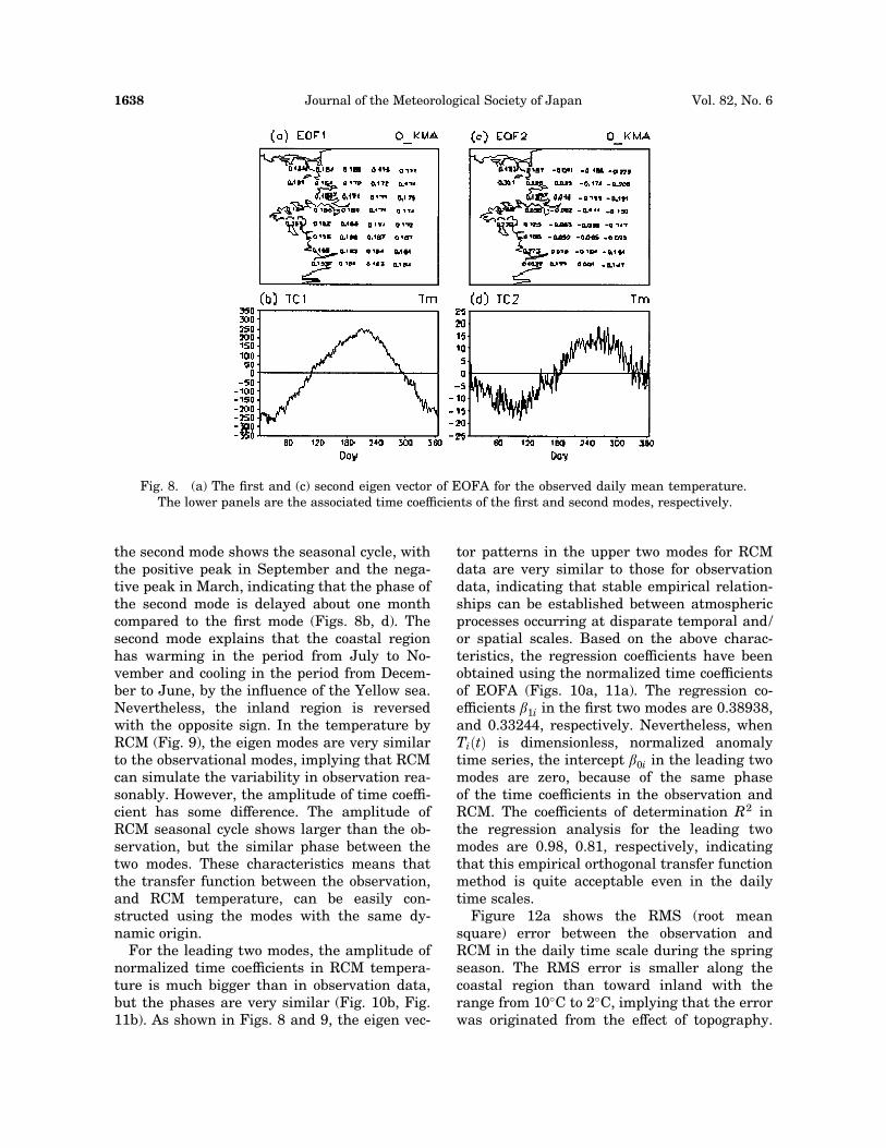
the second mode shows the seasonal cycle, withthe positive peak in September and the nega-tive peak in March, indicating that the phase ofthe second mode is delayed about one monthcompared to the first mode (Figs. 8b, d). Thesecond mode explains that the coastal regionhas warming in the period from July to No-vember and cooling in the period from Decem-ber to June, by the influence of the Yellow sea.Nevertheless, the inland region is reversedwith the opposite sign. In the temperature byRCM (Fig. 9), the eigen modes are very similarto the observational modes, implying that RCMcan simulate the variability in observation rea-sonably. However, the amplitude of time coeffi-cient has some difference. The amplitude ofRCM seasonal cycle shows larger than the ob-servation, but the similar phase between thetwo modes. These characteristics means thatthe transfer function between the observation,and RCM temperature, can be easily con-structed using the modes with the same dy-namic origin.

For the leading two modes, the amplitude ofnormalized time coefficients in RCM tempera-ture is much bigger than in observation data,but the phases are very similar (Fig. 10b, Fig.11b). As shown in Figs. 8 and 9, the eigen vec-

tor patterns in the upper two modes for RCMdata are very similar to those for observationdata, indicating that stable empirical relation-ships can be established between atmosphericprocesses occurring at disparate temporal and/or spatial scales. Based on the above charac-teristics, the regression coefficients have beenobtained using the normalized time coefficientsof EOFA (Figs. 10a, 11a). The regression co-efficients b1i in the first two modes are 0.38938,and 0.33244, respectively. Nevertheless, whenTiðtÞ is dimensionless, normalized anomalytime series, the intercept b0i in the leading twomodes are zero, because of the same phaseof the time coefficients in the observation andRCM. The coefficients of determination R2 inthe regression analysis for the leading twomodes are 0.98, 0.81, respectively, indicatingthat this empirical orthogonal transfer functionmethod is quite acceptable even in the dailytime scales.

Figure 12a shows the RMS (root meansquare) error between the observation andRCM in the daily time scale during the springseason. The RMS error is smaller along thecoastal region than toward inland with therange from 10�C to 2�C, implying that the errorwas originated from the effect of topography.

Fig. 8. (a) The first and (c) second eigen vector of EOFA for the observed daily mean temperature.The lower panels are the associated time coefficients of the first and second modes, respectively.


The RMS error is significantly reduced aftercorrecting the systematic bias based on thetransfer function. It is below 2�C, even in thelargest error region (Fig. 12a). The distributionof RMS error in the summer is quite similar tothat in the spring expect for the largest RMSerror among the all season, with the range from3 to 17�C (Fig. 12b). The corrected RMS errorhas the range from 0.8 to 2.5�C, which is just

about 5–20% of the original RMS error (Fig.12b). The RMS error patterns in fall and winterare very similar to these in summer and spring,indicating that the RMS error is systematic,thus to be corrected (Figs. 12c, d). The RMSerror after the correction is very small com-pared to the original RMS error. It is below 2�Cin the annual mean.

The effect of correction using the transfer

Fig. 9. Same as in Fig. 8 except for the RCM daily mean temperature.

Fig. 10. (a) Scatter diagram of the time coefficients of the first mode in EOFA between RCM andobservation for daily mean temperature in Korea. The regression line (solid line), equation and thecoefficient of determination (RSQ) are also indicated in (a). (b) As in (a) except for the time series.The lines in (b) indicate RCM, observation and the correction by transfer function, respectively.


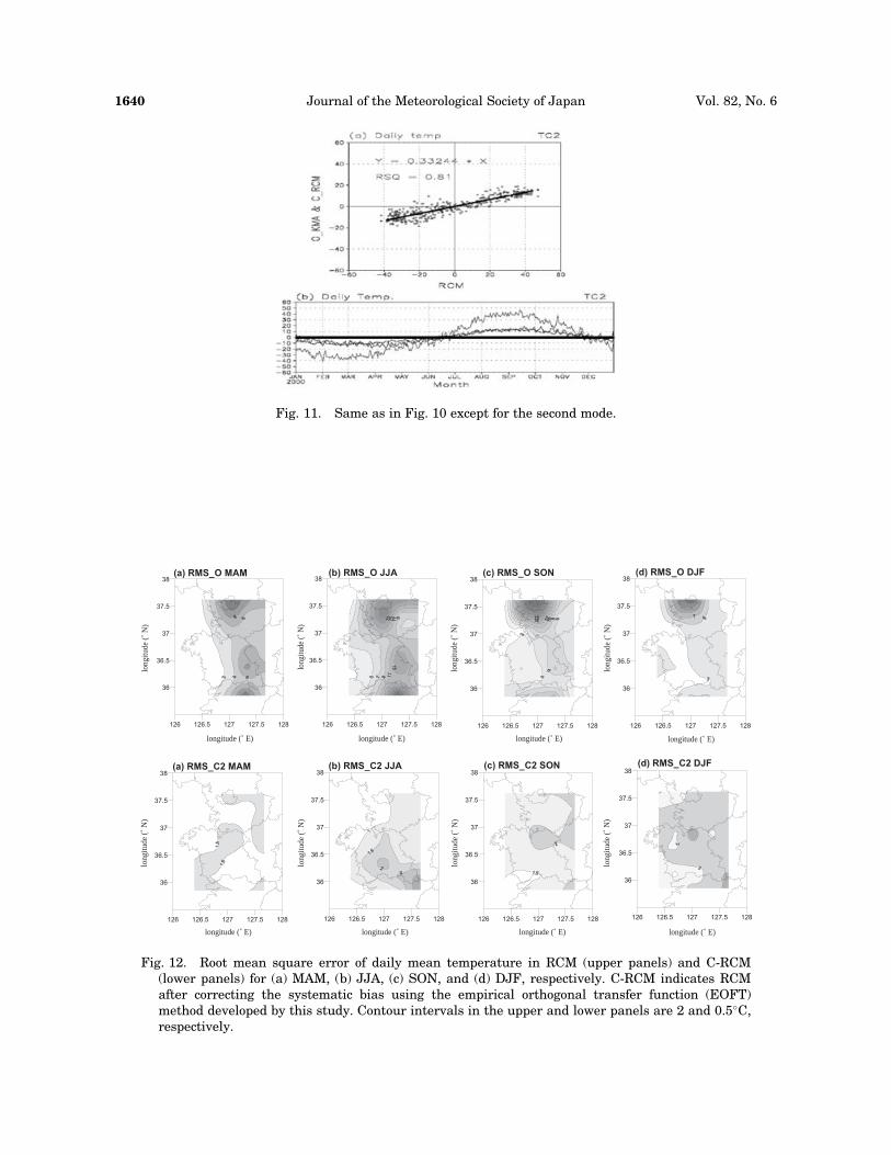
Fig. 11. Same as in Fig. 10 except for the second mode.

126 126.5 127 127.5 128

36

36.5

37

37.5

38

126 126.5 127 127.5 128

36

36.5

37

37.5

38

126 126.5 127 127.5 128

36

36.5

37

37.5

38

126 126.5 127 127.5 128

36

36.5

37

37.5

38

126 126.5 127 127.5 128

36

36.5

37

37.5

38

126 126.5 127 127.5 128

36

36.5

37

37.5

38

126 126.5 127 127.5 128

36

36.5

37

37.5

38

126 126.5 127 127.5 128

36

36.5

37

37.5

38

(a) RMS_O MAM (b) RMS_O JJA (c) RMS_O SON (d) RMS_O DJF

(d) RMS_C2 DJF(c) RMS_C2 SON(b) RMS_C2 JJA(a) RMS_C2 MAM

longitude (˚ E) longitude (˚ E) longitude (˚ E)

longitude (˚ E)longitude (˚ E) longitude (˚ E)

long

itude

(˚ N

)

long

itude

(˚ N

)

long

itude

(˚ N

)lo

ngitu

de (˚

N)

long

itude

(˚ N

)

long

itude

(˚ N

)

long

itude

(˚ N

)

long

itude

(˚ N

)

longitude (˚ E)

longitude (˚ E)

Fig. 12. Root mean square error of daily mean temperature in RCM (upper panels) and C-RCM(lower panels) for (a) MAM, (b) JJA, (c) SON, and (d) DJF, respectively. C-RCM indicates RCMafter correcting the systematic bias using the empirical orthogonal transfer function (EOFT)method developed by this study. Contour intervals in the upper and lower panels are 2 and 0.5�C,respectively.


function is summarized in Table 3. RMS errorof the daily mean temperature in RCM usedhas the range from 4.03 in winter to 9.70�C insummer, the biggest cold bias in summer. RMSerror of daily mean temperature in RCM is sig-nificantly reduced after a correction based onthe transfer function. Corrected percentage inRMS error has the range from 47.6 in winter to86.5% in summer, indicating that the empiricalorthogonal transfer function (EOTF) method,developed in this study, is very useful evenin daily time scale. But, climate change mostlymeans the difference, not the variable valuesthemselves, implying that systematic biasmay cancel between different periods. Table 4shows the difference between with adjustment,and without adjustment in daily mean temper-ature. Actually the difference in climate changebetween the two methods is reduced in com-parison with the difference in the currentclimate. The difference between two climatechanges has the range from �8.7% in fall to28.8% in winter, relative to the temperature

change from dynamic downscaling. These re-sults suggest that although systematic bias cancancel between two periods, statistical adjust-ment is also important to reduce the modelbias.

5. Conclusion

By combining dynamic downscaling and sta-tistical adjustment, we may provide reasonablefuture regional climate information from globalclimate model simulations. The final outputof temperature is quite adequate for regionalassessment studies change, since there are dis-tinguished variation modes influenced by landand ocean. Precipitation, however, has a lotof room to be improved. There are somewhatdisagreement in dominant modes of real worldand model world. This may be caused not onlyfrom the fact that precipitation is a local phe-nomena, and less systematic than temperature,but also the model has still treated the pre-cipitation processes inadequately. This mightbe one of important tasks of future studies, toovercome and provide reasonable regional cli-mate change information.

Through this study, we have learned that theadjustment of land surface temperature takesquite a long period. The cold bias generated bythe RCM has remained, with almost the origi-nal gap through 30 years integration. Accord-ingly, it might be necessary to apply the spin-up procedure for land surface in the RCM,before long-term integration. It may providemore reasonable regional climate change infor-mation, and less statistical adjustment.

Acknowledgement

The authors are grateful to reviewers fortheir helpful comments on the manuscript. Thisresearch was performed as a project of theKorean Meteorological Research Institute, ‘‘Re-

Table 3. RMS error (�C) of daily meantemperature in Korea. RCM_C1 andRCM_C12 indicate RMS errors aftercorrecting the first mode and the lead-ing two modes, respectively.

RMSerror

season RCM RCM_C1 RCM_C12

Correctedpercent-age (%)

spring 4.73 1.78 1.48 68.7

summer 9.70 1.45 1.31 86.5

autumn 6.64 2.20 1.86 72.0

winter 4.03 2.16 2.11 47.6

annual 6.29 1.90 1.69 73.1

Table 4. The difference between statistical adjustment and dynamicdownscaling in the daily mean temperature change between 1992–2002 and 2021–2030. The difference is indicated as the percentagerelative to dynamic downscaling.

difference spring summer autumn winter annual

Minimum �14.9 �12.3 �8.7 �17.2 �12.5

Maximum 17.8 15.2 10.6 28.8 13.4


search on the Development of Regional ClimateChange Scenarios to Prepare the National Cli-mate Change Report (I).’’

References

Bacher, A., J.M. Oberhuber and E. Roeckner, 1998:ENSO dynamics and seasonal cycle in thetropical Pacific as simulated by the ECHAM4/OPYC3 coupled general circulation model.Clim. Dyn., 14, 431–450.

Baquero-Bernal, A., M. Latif and S. Legutke, 2002:On dipolelike variability of sea surface tem-perature in the tropical Indian Ocean. J. Cli-mate, 15, 1358–1368.

Cubasch, U., J. Waszkewitz, G. Hegerl and J. Perl-witz, 1995: Regional climate changes as simu-lated in time-slice experiments. Clim. Change,31, 273–304.

Deque, M. and J.P. Piedelievre, 1995: High resolu-tion climate simulation over Europe. Clim.Dyn., 11, 321–339.

Dickinson, R.E., R.M. Errico, F. Giorgi and G.T.Bates, 1989: A regional climate model forwestern United States. Clim. Change, 15, 383–422.

Feddersen, H., A. Navarra and M.N. Ward, 1999:Reduction of model systematic error by statis-tical correction for dynamic seasonal predic-tion. J. Climate, 12, 1974–1989.

Giorgi, F., 1990: Simulation of regional climate usinga limited area model nested in a general circu-lation model. J. Climate, 3, 941–963.

Gong, W.S., 2001: Temporal and spatial changes inthe distribution of Phyllostachys habitation.Kor. Geograph. Soc., 36, 444–457 (in Korean).

Hong, S.-Y. and H.-M. Juang, 1998: Orographyblending in the lateral boundary of a regionalmodel. Mon. Wea. Rev., 126, 1714–1718.

IPCC, 1996: Climate change 1995: The Scienceof Climate Change. Contribution of WorkingGroup I to the Second Assessment Report of theIntergovernmental Panel on Climate Change[J.T. Houghton, L.G. Meira Filho, B.A. Call-ander, N. Harris, A. Kattenberg and K. Mas-kell (eds.)], Cambridge University Press, Cam-bridge, 572pp.

IPCC, 2000: Special Report on Emissions Sce-narios, Nakicenovic, Nebojsa and Swart, Rob(eds.), Cambridge University Press, Cam-bridge, United Kingdom, 612pp.

IPCC, 2001: Climate Change 2001: The ScientificBasis. Contribution of Working Group I to theThird Assessment Report of the Intergovern-mental Panel on Climate Change (IPCC) J.T.Houghton, Y. Ding, D.J. Griggs, M. Noguer,

P.J. van der Linden and D. Xiaosu (Eds.) Cam-bridge University Press, UK. 944pp.

Kim, J.W., J.T. Chang, N.L. Barker, D.S. Wilks andW.L. Gates, 1984: The statistical problem ofclimate inversion: Determination of the rela-tionship between local and large-scale climate.Mon. Wea. Rev., 112, 2069–2077.

Kim, M.-K., I.-S. Kang, C.-K. Park and K.M. Kim,2004: Super ensemble prediction of regionalprecipitation over Korea. Intl. J. Climatol., 24,777–790.

Legutke, S. and R. Voss, 1999: The Hamburgatmosphere-ocean coupled circulation modelECHO-G. Technical report No. 18, GermanClimate Computer Center (DKRZ), Hamburg,Germany, 62pp.

Oh, J.-H. and D.-Y. Kang, 2004: Climate changeduring 20th century at Busan, Korea (whichcan be obtained by e-mail to [email protected])(to be submitted).

Oh, J.-H., M.-K. Kim, S.-H. Lee and T.-K. Kim, 2002:‘‘Development on regional climate change sce-narios for Korea peninsula and East Asia’’,Meteorological Research Institute, KMA,Seoul, Korea, 212pp (in Korean) (which can beobtained by e-mail to [email protected]).

Roeckner, E., J.M. Oberhuber, A. Bacher, M. Chris-toph, I. Kirchner, 1996a: ENSO variabilityand atmospheric response in a global coupledatmosphere-ocean GCM. Clim. Dyn., 12, 737–754.

Roeckner, E., K. Arpe, L. Bengtsson, M. Christoph,M. Claussen, L. Dumenil, M. Esch, M. Gior-getta, U. Schlese and U. Schulzweida, 1996b:The atmospheric general circulation modelECHAM-4: model description and simulation ofpresent-day climate. Report No. 218, the MaxPlanck Institute for Meteorology, Hamburg,Germany.

Roeckner, E., L. Bengtsson and J. Feichter, 1999:Transient climate change simulations with acoupled atmosphere-ocean GCM including thetropospheric sulfur cycle. J. Climate, 12, 3004–3032.

Stendel, M., T. Schmith, E. Roeckner and U.Cubasch, 2002: The climate of the 21st cen-tury: Transient simulations with a coupledatmosphere-ocean general circulation model.Revised version, Climate Centre Report 02-1,Danish Meteorological Insitute, Denmark,50pp.

Stratton, R.A. 1999: A high resolution AMIP inte-gration using the Hadley Centre model Had-AM2b. Clim. Dyn., 15, 9–28.

Ward, M.N. and A. Navarra, 1997: Pattern analysisof SST-forced variability in ensemble GCM


simulations: Examples over Europe and tropi-cal Pacific. J. Climate, 10, 2210–2220.

Wigley, T.M.L., P.D. Jones, K.R. Briffa and G.Smith, 1990: Obtaining sub-grid-scale infor-mation from coarse-resolution general circula-tion model output. J. Geophys. Res., 95(D2),1943–1953.

Wilby, R.L., T.M.L. Wigley, D, Conway, P.D. Jones,B.C. Hewitson, J. Main and D.S. Wilks, 1998:

Statistical downscaling of general circulationmodel output: A comparison of methods. Water.Resour. Res. 33(11), 2995–3008.

Zorita, E., F. Gonzalez-Rouco and S. Legutke, 2003:Testing the Mann et al. (1998) approach to pa-leoclimate reconstructions in the context of a1000-yr control simulation with the ECHO-Gcoupled climate model. J. Climate, 16, 1378–1390.


regional climate simulation for korea using dynamic

Documents