regional climate change scenarios for vulnerability and adaptation assessments

REGIONAL CLIMATE CHANGE SCENARIOS FOR VULNERABILITYAND ADAPTATION ASSESSMENTS

JOEL B. SMITH and GREGORY J. PITTSHagler Bailly Consulting, Inc., P.O. Drawer O, Boulder, CO 80306-1906, U.S.A.

Abstract. This paper describes the regional climate change scenarios that are recommended for usein the U.S. Country Studies Program (CSP) and evaluates how well four general circulation models(GCMs) simulate current climate over Europe. Under the umbrella of the CSP, 50 countries withvarying skills and experience in developing climate change scenarios are assessing vulnerabilityand adaptation. We considered the use of general circulation models, analogue warm periods, andincremental scenarios as the basis for creating climate change scenarios. We recommended thatparticipants in the CSP use a combination of GCM based scenarios and incremental scenarios. TheGCMs, in spite of their many deficiencies, are the best source of information about regional climatechange. Incremental scenarios help identify sensitivities to changes in a particular meteorologicalvariable and ensure that a wide range of regional climate change scenarios are considered. Werecommend using the period 1951–1980 as baseline climate because it was a relatively stable climateperiod globally. Average monthly changes from the GCMs and the incremental changes in climatevariables are combined with the historical record to produce scenarios. The scenarios do not considerchanges in interannual, daily, or subgrid scale variability. Countries participating in the CountryStudies Program were encouraged to compare the GCMs’ estimates of current climate with actuallong-term climate means. In this paper, we compare output of four GCMs (CCCM, GFDL, UKMO,and GISS) with observed climate over Europe by performing a spatial correlation analysis fortemperature and precipitation, by statistically comparing spatial patterns averaged climate estimatesfrom the GCMs with observed climate, and by examining how well the models estimate seasonalpatterns of temperature and precipitation. In Europe, the GISS and CCCM models best simulatecurrent temperature, whereas the GISS and UK89 models, and the CCCM model, best simulateprecipitation in defined northern and southern regions, respectively.

1. Introduction

The U.S. Country Studies Program (CSP) is providing financial and technicalassistance to more than 50 developing countries and countries with economies intransition to study climate change. These countries are being given guidance onhow to estimate their emissions of greenhouse gases, assess policies to mitigateemissions of greenhouse gases, and assess their vulnerability to climate changeand options for adapting to climate change. The studies are intended to provideuseful information about climate change to regional, national, and internationalpolicymakers.

This paper discusses the approach the CSP recommends on selecting and apply-ing climate change scenarios, and explores an approach for selecting general cir-culation models (GCMs) based on how well they estimate the observed currentclimate of Europe.

Climatic Change 36: 3–21, 1997.c 1997 Kluwer Academic Publishers. Printed in the Netherlands.

4 JOEL B. SMITH AND GREGORY J. PITTS

2. Why Are Climate Change Scenarios Needed?

If we knew exactly how regional climate was going to change in the future becauseof increased greenhouse gas concentrations, we could use those projections toestimate future impacts of climate change. Unfortunately, there is a tremendousamount of uncertainty about change in regional climate (Houghton et al., 1996).Since we cannot predict regional climate change, we use scenarios of climatechange to help identify the sensitivity, or vulnerability, of systems to climate change.Scenarios are plausible and internally consistent combinations of circumstancesused to represent potential future conditions (Carter et al., 1994).

3. Criteria for Selecting Climate Change Scenarios

In selecting climate change scenarios to be recommended for use in the CSP, wehad to keep the needs of a number of users in mind:

� Policymakers. Climate change scenarios need to accurately reflect the potentialmagnitude of climate change, but also the uncertainties and range of potentialclimate change on a regional scale.

� Impacts Assessors. Scenarios need to provide information on spatial andtemporal scales consistent with impacts assessment methods. Some methodsrequire daily inputs at a spatial scale as small as a farmer’s field.

� Country Studies Participants. The capabilities of researchers participatingin the CSP vary widely. Some researchers have already conducted impactsassessments, whereas others were, when they began the program, novices.With more than 50 countries involved, the ability to provide direct technicalassistance to all countries was limited. The scenarios had to be relatively easyto apply.

Selecting scenarios to be useful for policymakers affects the range of scenariosto be used. Selecting scenarios to be useful for impacts assessors influences thelevel of detailed outputs of the scenarios need to have. Selecting scenarios usefulfor Country Studies participants affects the level of sophistication necessary forresearchers to create the scenarios.

In addition to satisfying the needs of different audiences mentioned above, thescenarios must meet as many of the following criteria as possible.

REGIONAL CLIMATE CHANGE SCENARIOS 5

Table ICriteria satisfaction by scenario option

Criteria GCMs Analogue Incremental

Consistent withglobal predictions Yes No NoInternally consistent Yes Yes NoSufficient variables Yes Yes and no YesRange of estimate Somewhat No Yes

� The scenarios should be consistent with widely accepted global estimatesof climate change. The Intergovernmental Panel on Climate Change (IPCC)estimates that a doubling of carbon dioxide (CO2) in the atmosphere will leadto a 1 to 3.5 �C warming by 2100 (Houghton et al., 1996).�

� The scenarios should be physically plausible and internally consistent. Changesin meteorological variables need to be physically consistent. For example,increases in precipitation should be correlated with increases in cloudiness.

� The scenarios should estimate a sufficient number of variables at a spatialand temporal scale suitable for use in vulnerability assessment models (Vinerand Hulme, 1992). The scenarios need to provide daily estimates of changesin climate variables at a local spatial scale.

� The scenarios should reflect a regional range of potential climate change. Thescenarios should account for uncertainty about the direction and magnitude ofchange in such meteorological variables as temperatures and precipitation.

4. Options for Creating Climate Change Scenarios

We considered three sources of information for recommending climate change sce-narios to the countries in the CSP: GCMs, analogue warm periods, and incrementalscenarios. How well these three options meet the criteria for selection is displayedin Table I.

GCMs are mathematical representations of many atmosphere, ocean, and landsurface processes based on the laws of physics. Such models consider a wide rangeof physical processes that characterize the climate system and have been used toexamine the impact of increased greenhouse gas concentrations on global climate(Gates et al., 1990). GCMs estimate changes for dozens of meteorological variablesin regional climate in grid boxes that are typically 3 or 4 degrees in latitude and asmuch as 10 degrees in longitude.

� The Country Studies Program began in 1993, when the best information was that the most likelyrate of warming was 3 �C by 2100 (Houghton et al., 1992).


The advantage of using GCMs is that they fully or partially satisfy all four criteriafor selecting scenarios. GCMs have been run with increased greenhouse gases.Usually they are run assuming a doubling of CO2 concentrations in the atmosphere(2 � CO2) over mid-century conditions (1 � CO2). Some runs have been madeassuming a gradual (transient) increase in greenhouse gas concentrations. Thus,the regional estimates of climate change are consistent with the global changesin climate caused by greenhouse gas concentration increases. GCMs solve forfundamental laws of physics and, thus, estimated changes in regional climatevariables are roughly consistent. GCMs provide estimates of daily changes innumerous variables at the grid box scale, although only monthly data are providedas part of the U.S. Climate Change Program (Benioff et al., 1996). As is discussedbelow, relatively simply techniques can be used to create daily climate changescenarios at a local scale based on this output from the GCMs. GCMs reflect arange of climate change, but tend to be on the high side of a 2.5 �C warming (Gateset al., 1992).

One major disadvantage of GCMs is that they do not accurately representcurrent climate at a regional scale (Grotch and MacCracken, 1991; Kalkstein,1991; Robock et al., 1993). In many cases, basic seasonal patterns of precipitationare misrepresented. Thus, GCMs are not considered reliable enough to providepredictions of regional climate change.

Analogue Warm Periods are periods in the past when climate was warmer thannow for a sustained period of time. The 1930s in the central United States was about0.5 �C warmer than the 1951–1980 climate (Karl et al., 1994). The mid-Holoceneperiod – 6,000 to 9,000 years ago – was about 1 �C warmer over the NorthernHemisphere (Webb, 1992). The advantage of the analogues is that they providephysically consistent changes in regional climate and can do so at a finer scale thanGCMs, satisfying criterion 2. For example, daily weather data for many observingstations in the United States exists for the 1930s (Rosenberg et al., 1993).

The disadvantage of analogue warm periods is that they were most likely causedby forcings other than increased greenhouse gas concentrations. Paleoclimaticwarm periods such as the mid-Holocene were probably caused by changes in theEarth-Sun orbital parameters (COHMAP, 1988). It is uncertain why the 1930swere so warm. In addition, the analogue warm periods tend to have a relativelylow degree of global warming, around 1 �C,� and thus do not reflect a broad rangeof potential climate change. Thus, they do not satisfy criteria 1 and 4. Finally, datafor these analogue scenarios may not exist in many countries participating in theCSP, and these scenarios thus do not fully meet criterion 3.

� One could use analogue warm periods from at least several million years ago. However, thequality and the resolution of these data are limited.


The third option is incremental scenarios. These are also referred to as arbitrarychanges in climate and usually involve uniform changes in annual climate such as+2� and +4 �C combined with no change in precipitation or� 10 and 20% changesin precipitation.� The advantage of incremental scenarios is that they can be used torepresent a wide range of potential climate change such as increased and decreasedprecipitation. In addition, these scenarios can be used to examine the sensitivity ofsectors to changes in a particular climate variable.

Since incremental changes are arbitrary, one cannot be sure that they are consis-tent with global climate change caused by increased greenhouse gases. In addition,incremental scenarios may include combinations of variables that are unlikely toactually happen (such as increased temperature and no monthly change in precipi-tation or assuming a uniform change in a variable over a large area).

5. Recommended Approach for Creating Climate Change Scenarios

We recommended that CSP countries use a combination of GCMs and incrementalscenarios. The GCMs provide the best information (although with many problems)about how regional climate may change. The incremental scenarios complement theGCM scenarios because they provide a wider range of potential climate change atthe regional scale and because they are useful in identifying sensitivities to changesin specific variables. This approach of using both GCMs and incremental scenarioshas been used in many vulnerability assessments (e.g., Poiani and Johnson, 1993;Strzepek and Smith, 1995). In a review of methods for creating climate changescenarios, Sulzman et al. (1995) recommended using both GCMs and incrementalscenarios to provide the best information about potential regional climate changeto policymakers.

Neither GCMs nor the incremental approaches by themselves yield estimates ofdaily climate at the high degree of resolution needed for impacts assessment. Werecommended that these approaches be combined with an observed daily climatedata set to yield a scenario with sufficient spatial and temporal resolution. At least30 years of observed data should be used for this data set because that is theminimum number of years needed to define a climate. The years 1951–1980 arerecommended because they are a recent 30-year period and do not include the1980s (Carter et al., 1994). That decade included some of the warmest years onrecord in the last 130 years (Jones et al., 1994).�� This 30-year period also servesas baseline climate and is used to estimate how systems or resources perform underno climate change.

� One can introduce seasonal variation into incremental scenarios, as is being done for the CzechRepublic country study (Kalvova, J. and Nemesova, I.: 1995, ‘Czech Republic’s Climate ChangeScenario, The Country Study Version’, unpublished manuscript, Prague, Czech Republic: Faculty ofMathematics and Physics, Charles University).�� If data from the 1950s are not available or of poor quality, it is acceptable to use the period

1961–1990 as the base period.


Average monthly changes from the GCMs are combined with the appropriatebaseline data (i.e., average January changes are combined with January observa-tions) to yield a scenario containing 30 years of data. Changes in temperature(2�CO2 � 1�CO2) are added to observations, and the ratio of monthly changesin precipitation (2�CO2=1�CO2) is multiplied by observed precipitation values.Average annual changes for the incremental scenarios are also combined with thedata in a similar manner.

There are a number of significant limitations to this approach for creatingclimate change scenarios. One important limitation is that this approach does notcapture changes in spatial and temporal variability. Since GCMs represent climatein grid boxes that are several hundred kilometers across, they do not representlocal climate conditions that may be caused by such features as mountains orland-ocean interfaces. For example, it is unlikely that precipitation will changeuniformly over mountainous areas. These scenarios also assume that the daily andinterannual pattern of climate in the baseline record will be repeated in the future.The frequency of days with precipitation does not change, only the intensity. Thesescenarios do not include potential changes in the frequency of extreme events suchas storms, hurricanes, floods, or droughts caused by changes in variance.

A second limitation is that since the GCMs do not represent observed regionalclimate very well, the validity of their estimates of regional climate change is indoubt. If they fail to represent even average temperatures and precipitation or currentseasonality of climate, can we believe their estimates of changes in seasonality?Combining GCM estimates with the observed data helps to partially correct thisproblem. Rather than use absolute values from the GCMs, we use only changesapplied to observed values.

The third limitation is that as GCMs are changed and improved, their estimatesof regional climate change can change significantly. Thus, studies based on aparticular set of GCMs may not stand the test of time. Many of the GCMs used inthe CSP were run in the late 1980s and early 1990s. The models were run assumingchanges only in greenhouse gas concentrations. Since that time, the importanceof sulfate aerosols in influencing the magnitude of global climate change and theregional variance of climate change has become apparent (e.g., Kiehl and Briegleb,1993; Taylor and Penner, 1994). Recent GCM runs (which were not available forthis round of Country Study vulnerability and adaptation assessments) show thatadding in sulfate aerosols with the greenhouse gas forcing results in a lower rateof average global warming and relatively much less warming in many mid-latitudeareas of the globe than when greenhouse gases alone are considered (e.g., Mitchellet al., 1995).

Researchers need to be sure to carefully explain these limitations of GCMs topolicymakers before presenting results of vulnerability analyses based on GCMscenarios. Policymakers should understand that results such as those from theCSP, although they are plausible, do not represent the true range of potentialclimate changes from global warming. They are scenarios in that they represent


plausible combinations of circumstances consistent with increased greenhouse gasconcentrations in the atmosphere. Other combinations of changes in climate mayalso happen. Nonetheless, these scenarios are quite useful for identifying potentialvulnerabilities to climate change.

6. Selection of GCMs

At least two to three GCMs should be used to create regional climate changescenarios (Benioff et al., 1996). This helps ensure that a variety of climate changescenarios are developed. (Incremental scenarios also help to ensure that a varietyof climate scenarios are used.) Because it is time consuming and expensive to runand analyze many climate change scenarios, it may be difficult for researchers touse more than several GCMs. We recommend that GCMs be selected on how wellthey represent current climate in the region of concern.

There are more than half a dozen GCMs available for use in vulnerabilityassessment (Benioff et al., 1996). The GCMs vary quite considerably in how wellthey estimate current climate; some GCMs simulate observed climates relativelywell in some regions, but perform relatively less well in other regions.

Countries in the CSP were urged to compare GCM estimates of current climatewith long-term climate means from observation stations in their countries andwith a set of spatially averaged (on a 4� � 5� grid) set of long-term climatemeans (Taljaard et al., 1969; Crutcher and Meserve, 1970; Schutz and Gates, 1971;Jaeger, 1976). This data set was compiled by the National Center for AtmosphericResearch (Benioff et al., in press) and is referred to as the CLIM data set. Thereis no guarantee that GCMs that best simulate current climate will best simulatechanges due to greenhouse gas forcing, but it is reasonable to use this process toselect GCMs to be used for creating scenarios.

7. Selection of GCMs for Europe

We compared four GCMs with the CLIM temperature and precipitation data� overEurope to assess the relative errors in the GCMs and to rank these four with regardto how well they simulate European climate as a whole. We compared the GCMswith observed climate in a rectangle bounded by 5� W and 30� E longitudes and42� N and 62� N latitudes. This area is approximately from western France toKiev, Ukraine, and from central Italy to St. Petersburg, Russia. Within this region,we found two distinct climates, approximately divided by the Alps. The northernsection of this region (48� N to 62� N) represents a continental climate with peak

� The CLIM data set includes only temperature and precipitation. Assessing GCM accuracy bycomparing pressure patterns estimated by the GCMs with observed pressure patterns would producemore reliable results.


precipitation in the summer, and the southern region (42� N to 47� N) defines aMediterranean climate with peak precipitation in the winter. We found significantseasonal pattern differences for precipitation across the regions, and, as a result,we report precipitation results for the northern and southern regions. We did notcompare the GCMs with specific countries or sites. The four GCMs are:

� Geophysical Fluid Dynamics Laboratory (GFDL). This model has a resolutionof 2:22� � 3:75� and projects an average global warming of 4 �C (Mitchell etal., 1990).

� Canadian Climate Centre Model (CCCM). This model has a resolution of3:75� � 3:75� and estimates that CO2 doubling will warm the earth by 3.5 �C(Boer et al., 1992).

� United Kingdom Meteorological Office (UK89). This model has a resolutionof 2:5� � 3:75� and results in an average global warming of 3.5 �C (Mitchellet al., 1990).

� Goddard Institute for Space Studies (GISS). This model has a resolution of7:83� � 10� and has an average global warming of 4.2 �C. This is the lowestresolution of the four models (Hansen et al., 1983).

We used three methods to compare the GCMs with observations. The firstinvolved performing a spatial correlation analysis of temperature and precipitationfor all months and on a yearly basis between the GCM output and the CLIM data.The second involved comparing spatially averaged temperature and precipitationestimates for Europe from the GCMs and the CLIM data base using the root meansquare error (RMSE) statistic. The third method involved checking the models’abilities to reflect seasonality by plotting and comparing spatially averaged timeseries precipitation and temperature values for the GCMs against actual seasonalityin the CLIM data.

7.1. SPATIAL PATTERN CORRELATION ANALYSIS

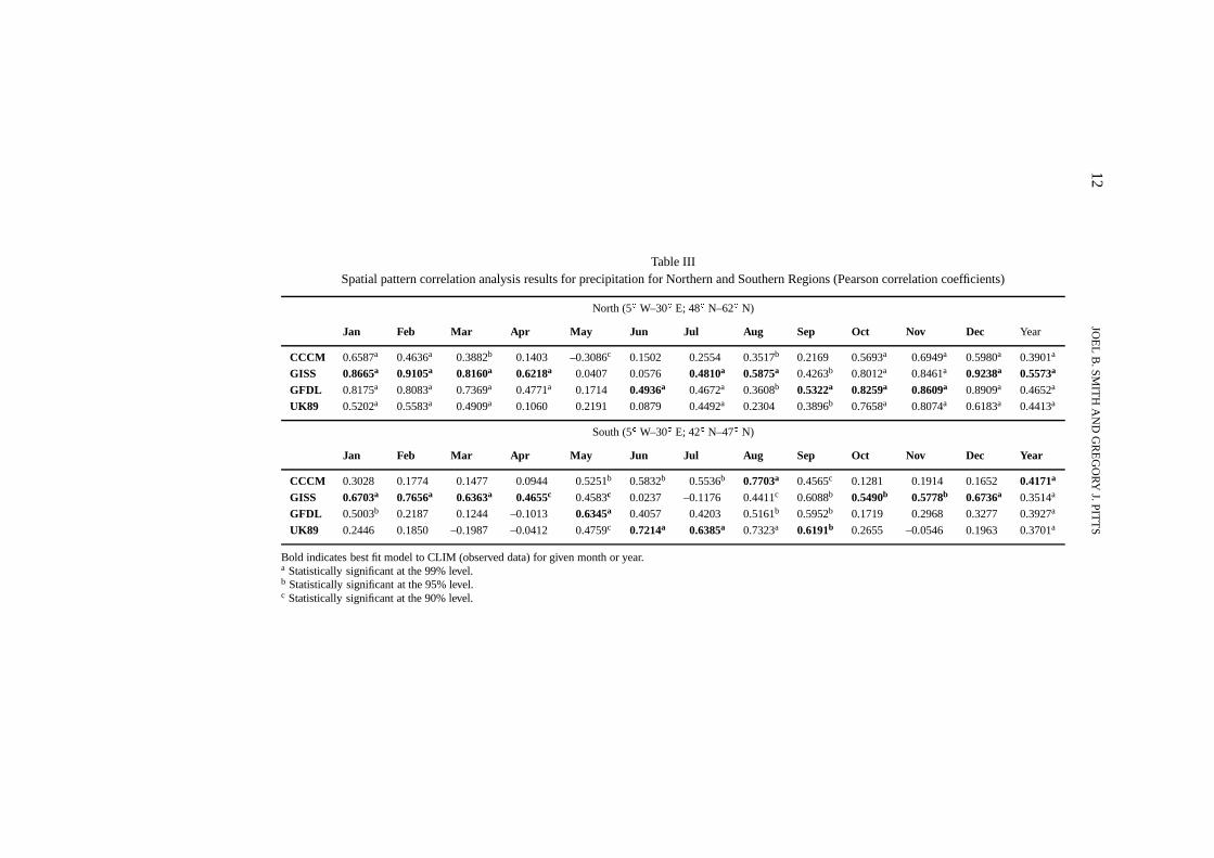
Using SASr (SAS Institute Inc., 1989), we calculated Pearson correlation coef-ficients between CLIM and the GCMs to determine how well each of the GCMsmodels the observed data. These correlation coefficients were calculated using grid-cell by gridcell data� for each month and for the entire year. Tables II and III reportthe Pearson correlation coefficients for temperature and precipitation, respectively,indicating the statistical significance of the results. The observed long-term averageJanuary precipitation in Europe is displayed in Figure 1a. Figures 1b through 1edisplay the GCMs’ estimates of current January precipitation over the region.

Although all models do well, the GISS model reflects the general temperaturepatterns best in all months and for the year for the region. The CCCM has the secondhighest spatial pattern correlation coefficient on an annual basis and for six months.

� The data were latitudinally weighted using the weighting subroutine GZONE-WT, version 1.3(1/21/91), programmed by Havey Davies.

RE

GIO

NA

LC

LIM

AT

EC

HA

NG

ESC

EN

AR

IOS

11

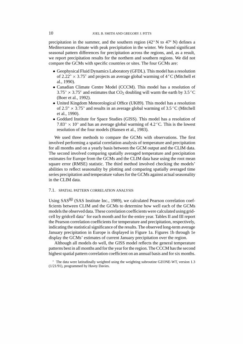
Table IISpatial pattern correlation analysis results for temperature for Europe (Pearson correlation coefficients)

Jan Feb Mar Apr May Jun Jul Aug Sep Oct Nov Dec Year

CCCM 0.9344a 0.9548a 0.9382a 0.9188a 0.8979a 0.8794a 0.8770a 0.8972a 0.9083a 0.9254a 0.9089a 0.9022a 0.9701a

GISS 0.9601a 0.9816a 0.9828a 0.9734a 0.9396a 0.9392a 0.9429a 0.9535a 0.9490a 0.9567a 0.9425a 0.9508a 0.9775a

GFDL 0.8723a 0.8850a 0.9176a 0.8687a 0.9043a 0.8585a 0.8575a 0.7938a 0.8044a 0.9441a 0.9315a 0.9157a 0.9611a

UK89 0.9050a 0.9236a 0.9115a 0.8474a 0.7973a 0.8472a 0.8919a 0.8894a 0.8720a 0.8403a 0.8612a 0.8952a 0.9284a

Bold indicates best fit model to CLIM (observed data) for given month or year.a Statistically significant at the 99% level.b Statistically significant at the 95% level.c Statistically significant at the 90% level.

12JO

EL

B.SM

ITH

AN

DG

RE

GO

RY

J.PITT

S

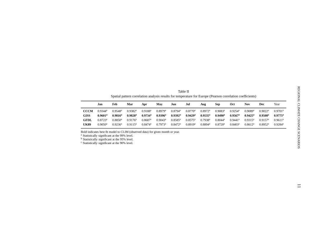
Table IIISpatial pattern correlation analysis results for precipitation for Northern and Southern Regions (Pearson correlation coefficients)

North (5� W–30� E; 48� N–62� N)


CCCM 0.6587a 0.4636a 0.3882b 0.1403 –0.3086c 0.1502 0.2554 0.3517b 0.2169 0.5693a 0.6949a 0.5980a 0.3901a

GISS 0.8665a 0.9105a 0.8160a 0.6218a 0.0407 0.0576 0.4810a 0.5875a 0.4263b 0.8012a 0.8461a 0.9238a 0.5573a

GFDL 0.8175a 0.8083a 0.7369a 0.4771a 0.1714 0.4936a 0.4672a 0.3608b 0.5322a 0.8259a 0.8609a 0.8909a 0.4652a

UK89 0.5202a 0.5583a 0.4909a 0.1060 0.2191 0.0879 0.4492a 0.2304 0.3896b 0.7658a 0.8074a 0.6183a 0.4413a

South (5� W–30� E; 42� N–47� N)


CCCM 0.3028 0.1774 0.1477 0.0944 0.5251b 0.5832b 0.5536b 0.7703a 0.4565c 0.1281 0.1914 0.1652 0.4171a

GISS 0.6703a 0.7656a 0.6363a 0.4655c 0.4583c 0.0237 –0.1176 0.4411c 0.6088b 0.5490b 0.5778b 0.6736a 0.3514a

GFDL 0.5003b 0.2187 0.1244 –0.1013 0.6345a 0.4057 0.4203 0.5161b 0.5952b 0.1719 0.2968 0.3277 0.3927a

UK89 0.2446 0.1850 –0.1987 –0.0412 0.4759c 0.7214a 0.6385a 0.7323a 0.6191b 0.2655 –0.0546 0.1963 0.3701a

Bold indicates best fit model to CLIM (observed data) for given month or year.a Statistically significant at the 99% level.b Statistically significant at the 95% level.c Statistically significant at the 90% level.


Figure 1a. Precipitation for CLIM in January.

Figure 1b. Precipitation for CCCM in January.


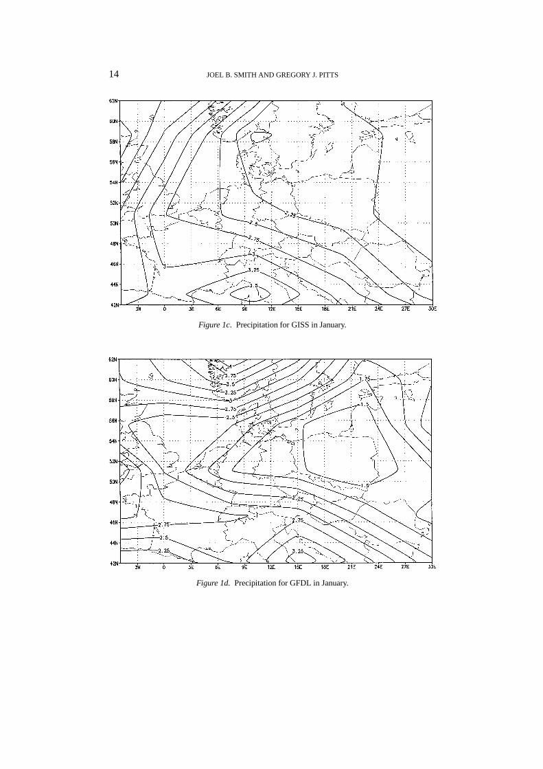
Figure 1c. Precipitation for GISS in January.

Figure 1d. Precipitation for GFDL in January.


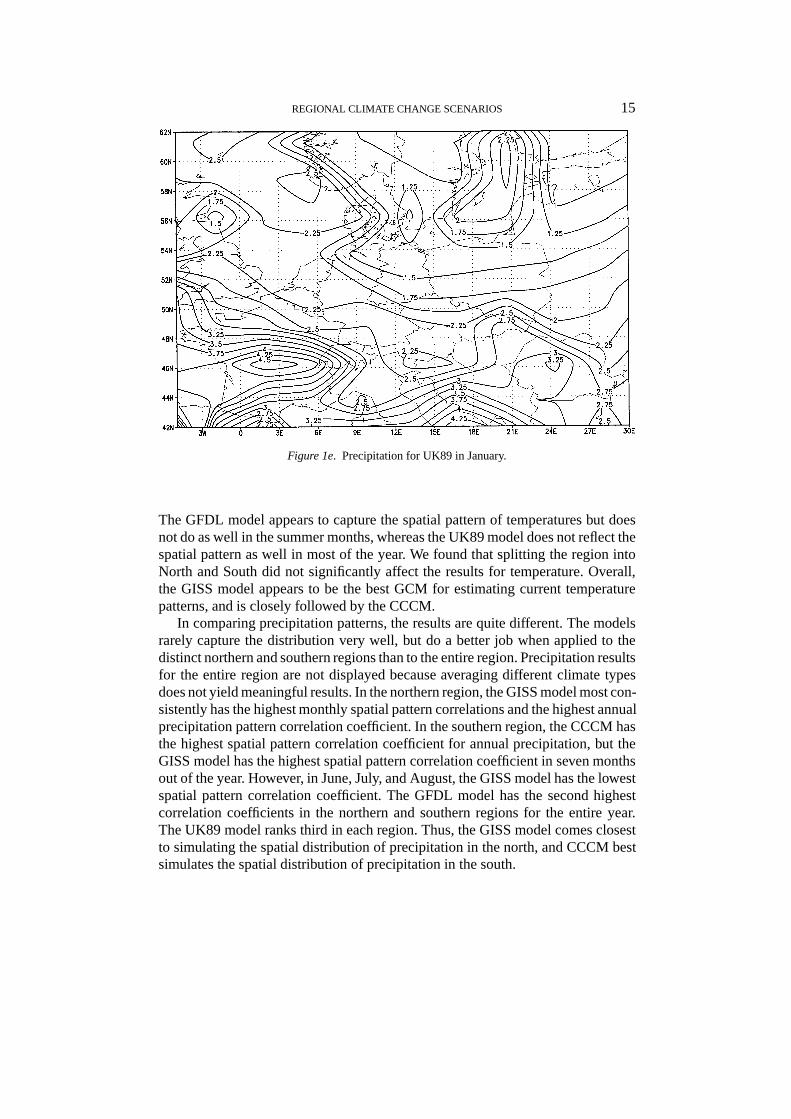
Figure 1e. Precipitation for UK89 in January.

The GFDL model appears to capture the spatial pattern of temperatures but doesnot do as well in the summer months, whereas the UK89 model does not reflect thespatial pattern as well in most of the year. We found that splitting the region intoNorth and South did not significantly affect the results for temperature. Overall,the GISS model appears to be the best GCM for estimating current temperaturepatterns, and is closely followed by the CCCM.

In comparing precipitation patterns, the results are quite different. The modelsrarely capture the distribution very well, but do a better job when applied to thedistinct northern and southern regions than to the entire region. Precipitation resultsfor the entire region are not displayed because averaging different climate typesdoes not yield meaningful results. In the northern region, the GISS model most con-sistently has the highest monthly spatial pattern correlations and the highest annualprecipitation pattern correlation coefficient. In the southern region, the CCCM hasthe highest spatial pattern correlation coefficient for annual precipitation, but theGISS model has the highest spatial pattern correlation coefficient in seven monthsout of the year. However, in June, July, and August, the GISS model has the lowestspatial pattern correlation coefficient. The GFDL model has the second highestcorrelation coefficients in the northern and southern regions for the entire year.The UK89 model ranks third in each region. Thus, the GISS model comes closestto simulating the spatial distribution of precipitation in the north, and CCCM bestsimulates the spatial distribution of precipitation in the south.


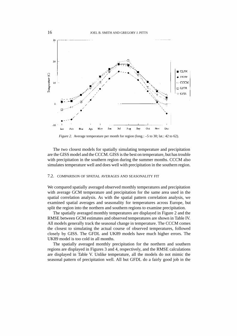
Figure 2. Average temperature per month for region (long.: –5 to 30; lat.: 42 to 62).

The two closest models for spatially simulating temperature and precipitationare the GISS model and the CCCM. GISS is the best on temperature, but has troublewith precipitation in the southern region during the summer months. CCCM alsosimulates temperature well and does well with precipitation in the southern region.

7.2. COMPARISON OF SPATIAL AVERAGES AND SEASONALITY FIT

We compared spatially averaged observed monthly temperatures and precipitationwith average GCM temperature and precipitation for the same area used in thespatial correlation analysis. As with the spatial pattern correlation analysis, weexamined spatial averages and seasonality for temperatures across Europe, butsplit the region into the northern and southern regions to examine precipitation.

The spatially averaged monthly temperatures are displayed in Figure 2 and theRMSE between GCM estimates and observed temperatures are shown in Table IV.All models generally track the seasonal change in temperature. The CCCM comesthe closest to simulating the actual course of observed temperatures, followedclosely by GISS. The GFDL and UK89 models have much higher errors. TheUK89 model is too cold in all months.

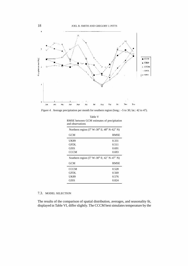
The spatially averaged monthly precipitation for the northern and southernregions are displayed in Figures 3 and 4, respectively, and the RMSE calculationsare displayed in Table V. Unlike temperature, all the models do not mimic theseasonal pattern of precipitation well. All but GFDL do a fairly good job in the


Table IVRMSE between GCM estimatesof temperature and observations,5� W–30� E; 42� N–62� N

GCM RMSE

CCCM 0.668GISS 1.363GFDL 2.858UK89 6.103

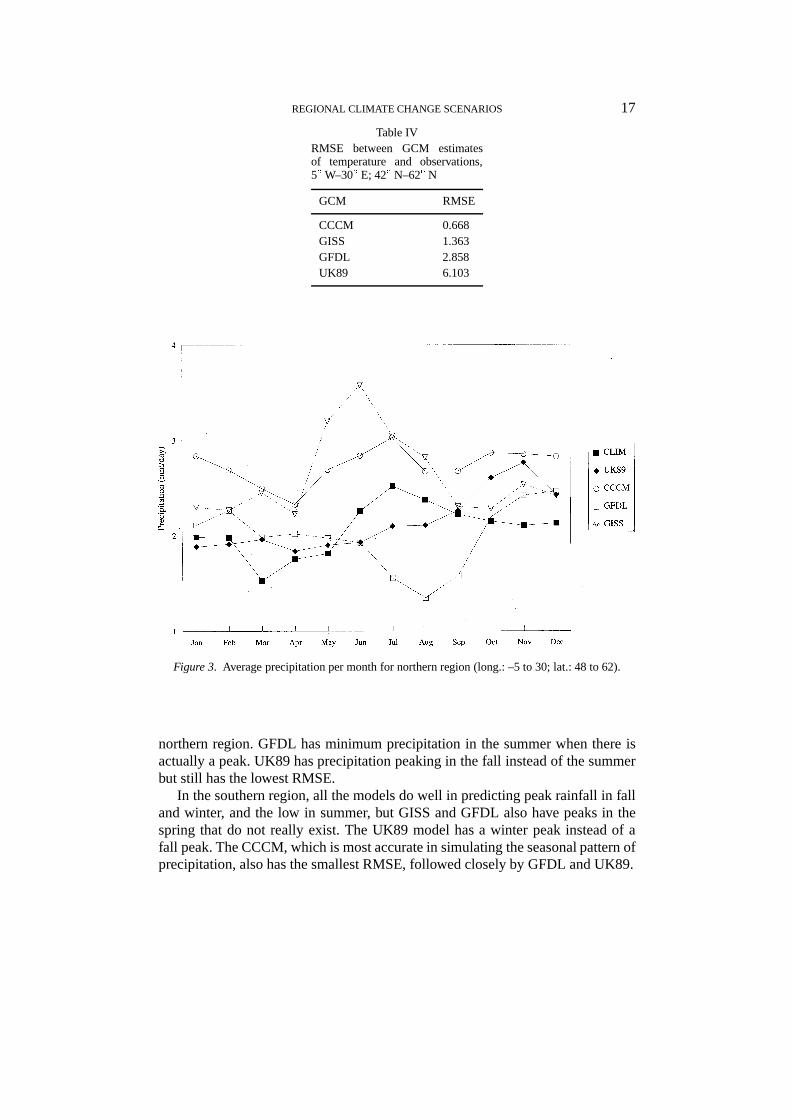
Figure 3. Average precipitation per month for northern region (long.: –5 to 30; lat.: 48 to 62).

northern region. GFDL has minimum precipitation in the summer when there isactually a peak. UK89 has precipitation peaking in the fall instead of the summerbut still has the lowest RMSE.

In the southern region, all the models do well in predicting peak rainfall in falland winter, and the low in summer, but GISS and GFDL also have peaks in thespring that do not really exist. The UK89 model has a winter peak instead of afall peak. The CCCM, which is most accurate in simulating the seasonal pattern ofprecipitation, also has the smallest RMSE, followed closely by GFDL and UK89.


Figure 4. Average precipitation per month for southern region (long.: –5 to 30; lat.: 42 to 47).

Table VRMSE between GCM estimates of precipitationand observations

Northern region (5� W–30� E; 48� N–62� N)

GCM RMSE

UK89 0.331GFDL 0.511GISS 0.691CCCM 0.693

Southern region (5� W–30� E; 42� N–47� N)

GCM RMSE

CCCM 0.528GFDL 0.569UK89 0.576GISS 0.824

7.3. MODEL SELECTION

The results of the comparison of spatial distribution, averages, and seasonality fit,displayed in Table VI, differ slightly. The CCCM best simulates temperature by the


Table VIBest fit model based on various goodness of fit parameters

Variable/test Spatial RMSE Seasonality Overallpatterncorrelation

Temperature GISS CCCM All CCCM & GISSPrecipitation North GISS UK89 All but GISS & UK89

GFDLSouth CCCM CCCM ALL CCCM

RMSE measure, but GISS is slightly superior on estimating spatial distributions.Both of the models seasonally fit very well. As for precipitation, the CCCM and theUK89 model appear to fit the seasonal precipitation patterns best, and in addition,UK89 has the smallest error in the northern region, and the CCCM has the smallesterror in the southern region. However, the CCCM has the greatest error in thenorthern region. On the whole, the CCCM does best in the southern region, but itis difficult to choose a best model in the northern region.

The models that best simulate current climate over Europe are CCCM andGISS. Comparatively, GFDL does not produce good results, and UK89 falls shortin most of the measures, except that it has the smallest RMSE for precipitationin the northern region. If two GCMs were to be selected for Europe, we wouldrecommend that they be the CCCM and GISS. To be sure, all the models havesignificant errors, and even those that ‘best’ simulate current climate should beused with caution.

8. Conclusions

We described a relatively simple approach for creating a set of climate changescenarios. We recommended using the outputs from GCMs and incremental sce-narios because this set of scenarios is consistent with estimated global climatechanges, is internally consistent, provides the data at a scale needed by vulnerabil-ity researchers, and provides a wide range of regional climate changes.

We also compared four GCMs with observed climate in Europe to determinewhich ones best represent current climate. This exercise does not ensure that thebest models have been selected. As noted above, just because GISS and CCCMhave the best fit does not mean they will be the best in estimating climate change.Other GCMs may better simulate observed temperature and precipitation patternsin other parts of the world.

In closing, it should be noted that all the GCMs make significant errors insimulating current climate. This may be due in part to the relatively low resolutionof the models, which limits their ability to simulate complex topography such as that


of Europe. Higher resolution in more recent GCMs and the use of such techniquesas nested models (Mearns et al., 1995) tend to result in more accurate estimationof current climate. The techniques we use here can still be used to examine theaccuracy of newer GCMs and approaches in simulating current climate.

Acknowledgments

We wish to acknowledge the hard work of Karen Richards, who helped us pullthis manuscript together, and Chris Thomas for editing the manuscript. We wishto thank Dr. Jaroslava Kalvova and Dr. Roy Jenne for their helpful comments.We also wish to thank two anonymous reviewers for their thoughtful comments.This work was funded by the U.S. Country Studies Program through a subcontractwith Argonne National Laboratory (contract number 941322403) and throughthe Energy Efficiency Project contract with the U.S. Agency for InternationalDevelopment (contract number PCE-5743-C-00-207300). We thank Robert Dixon,Ron Benioff, and Sandy Guill of the U.S. Country Studies Program for their supportof this effort.

References

Benioff, R., Guill, S., and Lee, J. (eds.).: (1996), Vulnerability and Adaptation Assessments: AnInternational Guidebook, Kluwer Academic Publishers, Dordrecht, p. 200.

Boer, G. J., McFarlane, N. A., and Lazare, M.: 1992, ‘Greenhouse Gas-Induced Climate ChangeSimulated with the CCC Second-Generation General Circulation Model’, Bull. Am. Meteor. Soc.5, 1045–1077.

Carter, T. R., Parry, M. L., Harasawa, H., and Nishioka, S.: 1994, IPCC Technical Guidelines forAssessing Climate Change Impacts and Adaptations, University College London, London, p. 59.

COHMAP: 1988, ‘Climatic Changes of the Last 18,000 Years: Observations and Model Simulations’,Science 241, 1043–1052.

Crutcher, H. L. and Meserve, J. M.: 1970, Selected Level Heights, Temperatures and Dew Points forthe Northern Hemisphere, Chief of Naval Operations, NAVAIR 50-1C-52 (revised), Washington,DC.

Gates, W. L., Rowntree, P. R., and Zeng, Q.-C.: 1990, ‘Validation of Climate Models’, in Houghton,J. T., Jenkins, G. J., and Ephraums, J. J. (eds.), Climate Change: The IPCC Scientific Assessment,Cambridge University Press, New York, p. 365.

Gates, W. L., Mitchell, J. F. B., Boer, G. J., Cubasch, U., and Meleshko, V. P.: 1992, ‘ClimateModeling, Climate Prediction and Model Validation’, in: Houghton, J. T., Callander, B. A.,and Varney, S. K., Climate Change 1992 – The Supplementary Report to the IPCC ScientificAssessment, WMO/UNEP Intergovernmental Panel on Climate Change, Cambridge UniversityPress, Cambridge, p. 200.

Grotch, S. L. and MacCracken, M. C.: 1991, ‘The Use of General Circulation Models to PredictRegional Climatic Change’, J. Clim. 4, 286–303.

Hansen, J., Russell, G., Rind, D., Stone, P., Lacis, A., Lebedeff, S., Ruedy, R., and Travis, L.: 1983,‘Efficient Three-Dimensional Global Models for Climate Studies: Models I and II’, Mon. Wea.Rev. 111, 609–622.

Houghton, J. T., Meira Filho, L. G., Callander, B. A., Harris, N., Kattenberg, A., and Maskell, K.(eds.): 1996, Climate Change 1995: The Science of Climate Change, Contribution of WorkingGroup I to the Second Assessment Report of the Intergovernmental Panel on Climate Change,Cambridge University Press, Cambridge, p. 572.


Houghton, J. T., Callander, B. A., and Varney, S. K.: 1992, Climate Change 1992 – The SupplementaryReport to the IPCC Scientific Assessment, WMO/UNEP Intergovernmental Panel on ClimateChange, Cambridge University Press, Cambridge, p. 200.

Jaeger, L.: 1976, ‘Monatskarten des Niederschlags fur die Ganze Erde’, Berichte des DeutschenWetterdienstes 139 (18).

Jones, P. D., Wigley, T. M. L., and Briffa, K. R.: 1994, ‘Global and Hemispheric TemperatureAnomalies – Land and Marine Instrumental Records’, in: Boden, T. A., Kaiser, D. P., Sepanski,R. J., and Stoss, F. W. (eds.), Trends ’93: A Compendium of Data on Global Change, Oak RidgeNational Laboratory, Oak Ridge, Tennessee, ORNL/CDIAC-65, p. 28.

Kalkstein, L. S. (ed.): 1991, Global Comparisons of Selected GCM Control Runs and ObservedClimate Data, U. S. Environmental Protection Agency, Washington, DC, p. 251.

Karl, T. R., Easterling, D. R., Knight, R. W., and Hughes, P. Y.: 1994, ‘U.S. National and RegionalTemperature Anomalies’, in: Boden, T. A., Kaiser, D. P., Sepanski, R. J., and Stoss, F. W. (eds.),Trends ’93: A Compendium of Data on Global Change, Oak Ridge National Laboratory, OakRidge, Tennessee, ORNL/CDIAC-65, p. 984.

Kiehl, J. T. and Briegleb, B. P.: 1993. ‘The Relative Roles of Sulfate Aerosols and Greenhouse Gasesin Climate Forcing’, Science 260, 311–314.

Mearns, L. O., Giorgi, F., Shields Brodeur, C., and McDaniel, L.: 1995, ‘Analysis of the Variabilityof Daily Precipitation in a Nested Modeling Experiment: Comparison with Observations and2� CO2 Results’, Global Planetary Change 10, 55–78.

Mitchell, J. F. B., Johns, T. C., Gregory, J. M., and Tett, S. F. B.: 1995, ‘Climate Response to IncreasingLevels of Greenhouse Gases and Sulphate Aerosols’, Nature 376, 501–504.

Mitchell, J. F. B., Manabe, S., Tokioka, T., and Meleshko, V.: 1990, ‘Equilibrium Change’, inHoughton, J. T., Jenkins, G. J., and Ephraums, J. J. (eds.), Climate Change: The IPCC ScientificAssessment, Cambridge University Press, Cambridge, p. 364.

Poiani, K. A. and Johnson, W. C.: 1993, ‘Potential Effects of Climate Change on a Semi-PermanentPrairie Wetland’, Clim. Change 24, 213–232.

Robock, A., Turco, R. P., Harwell, M. A., Ackerman, T. P., Andressen, R., Chang, H.-S., andSivakumar, M. V. K.: 1993, ‘Use of General Circulation Model Output in the Creation of ClimateChange Scenarios for Impact Analysis’, Clim. Change 23, 293–335.

Rosenberg, N. J., Crosson, P. R., Frederick, K. D., Easterling, W. E., McKenney, M. S., Bowes,M. D., Sedjo, R. A., Darmstadter, J., Katz, L. A., and Lemon, K. M.: 1993, ‘Paper 1: The MINKMethodology: Background and Baseline’, Clim. Change 24, 7–22.

SAS Institute Inc.: 1989, SAS/STAT User’s Guide, Version 6, Fourth Edition Volume 1, SAS Institute,Inc., Cary, NC.

Schutz, C. and Gates, W. L.: 1971, ‘Global Climate Data for Surface, 800 millibars, 400 millibars’,Rand Corporation, Santa Monica, California, R-915-ARPA, p. 173.

Strzepek, K. M. and Smith, J. B. (eds.).: 1995, As Climate Changes: International Impacts andImplications, Cambridge University Press, Cambridge, p. 213.

Sulzman, E. W., Poiani, K. A., and Kittel, T. G. F.: 1995, ‘Modeling Human-Induced Climatic Change:A Summary for Environmental Managers’, Environ. Mgmt. 19, 197–224.

Taljaard, J. J., van Loon, H., Crutcher, H. L., and Jenne, R. L.: 1969, Climate of the Upper Air:Southern Hemisphere. 1: Temperatures, Dewpoints, and Heights at Selected Pressure Levels,Chief of Naval Operations, Washington, D. C. NAVAIR 50-1C-55, p. 134.

Taylor, K. E. and Penner, J. E.: 1994, ‘Response of the Climate System to Atmospheric Aerosols andGreenhouse Gases’, Nature 369, 734–737.

Viner, D. and Hulme, M.: 1992, Climate Change Scenarios For Impact Studies in the UK, ClimaticResearch Unit, University of East Anglia, Norwich, p. 33.

Webb, T., III.: 1992, ‘Past Changes in Vegetation and Climate: Lessons for the Future’, in Peters,R. L. and Lovejoy, T. E. (eds.), Global Warming and Biological Diversity, Yale University Press,New Haven, CN, p. 386.

(Received 17 November 1995; in revised form 21 October 1996)

regional climate change scenarios for vulnerability and adaptation assessments

Documents