regime switching policy rules and economic growth the msc model is estimated using a matlab package...

PROSIDING PERKEM VII, JILID 2 (2012) 1562 – 1580

ISSN: 2231-962X

Persidangan Kebangsaan Ekonomi Malaysia ke VII (PERKEM VII)

Transformasi Ekonomi dan Sosial ke Arah Negara Maju

Ipoh, Perak, 4-6 Jun 2012

Regime Switching Policy Rules and Economic Growth

Norlin Khalid

Pusat Pengajian Ekonomi

Fakulti Ekonomi dan Pengurusan

Universiti Kebangsaan Malaysia

Email: [email protected]

Nur Fakhzan Marwan

Faculty of Business Management,

Universiti Teknologi MARA,

UiTM Pahang

ABSTRACT

This paper empirically examines the relative effect of active and passive regime policy rules on

economic growth. We use time series data for a set of South East Asian countries namely, Malaysia,

Thailand and Singapore for the period 1971-2009. The Markov-switching (MSC) regression method is

employed to characterize the regime switching change for both monetary and fiscal policy reaction

functions for each country. Rather than treating the policy rules as exogenous, the policy regime is

allowed to switch endogenously between active and passive. Then, the relative impact of these regime

policies on long run output growth is estimated by using Autoregressive Distributed Lag (ARDL)

method. Dummy variables are used to capture the difference in regime policies. The MSC regression

shows that Thailand‟s monetary policy was mostly active while fiscal policy was mostly passive

throughout the sample covered. When both policies are considered, we note that Thailand‟s changes

in policy regimes between periods are very frequent. In contrast, Singapore‟s regime switching is

quite more stable. Singapore was in active monetary and passive fiscal for 20 years from 1971 to

1991 and it took about 8 years being in regime passive monetary and passive fiscal before switched

to passive monetary and active fiscal in year 2000 until 2009. Nevertheless, Malaysia‟s monetary

policy regimes were characterized as passive at all times while fiscal regimes were active throughout

the sample study. Furthermore, the ARDL cointegration shows that both monetary and fiscal policies

through its instruments broad money and government spending respectively are important in sustaining

long run economic growth for Thailand. Meanwhile, Singaporean economy is only positively

determined by monetary policy while fiscal policy is insignificant. As for regime switching, our

results indicate that only dummy for monetary policy effect the economic growth in Thailand. This

implies an active monetary authority will only lead to a lower output growth. However, none of the

dummy variables are significant for Singapore which indicates that the characterization of policy

authority either active or passive is not really matter for economic growth.

Keywords: Monetary Policy; Fiscal Policy; Markov Regime Switching; Economic Growth

JEL Classification Numbers: E6, E12, E63, H3.

INTRODUCTION

The debate between monetary and fiscal policy is an old topic and has been discussed extensively in

macroeconomics between the Monetarist and Keynesian‟s schools of thoughts. There are a huge

number of studies on the relative effectiveness both of these policy rules on the output growth either

theoretically or empirically. Yet, to the best of our knowledge,1 despite the role of monetary and fiscal

policy rules on economic growth has been discussed widely, none of the literatures has discussed

specifically the effect of different regime of „active‟ vs. „passive‟ policy rules. This is crucial as many

previous empirical studies have found that the policy rules associated with monetary and fiscal were

switching overtime between „active‟ and „passive‟. Therefore, it is better to model monetary and fiscal

1 see for example Friedman and Meiselman (1963), Ansari (1996), Reynolds, A. (2000), Chari et al. (1991), Schmitt-Grohe

and Uribe (2001),Shapiro and Watson (1988), Blanchard and Quah (1989) and Clarida and Gali (1994), Nottage (2001), Chari and Kehoe (998), Kim (1997), Chowdhury (1988).

Prosiding Persidangan Kebangsaan Ekonomi Malaysia Ke VII 2012 1563

rules as a regime switching model than a model without regime switching. It is also suspected that

different regime of policy rules would affect the behavior of economic growth differently i.e.,

between regime of active monetary/passive fiscal versus regime of passive monetary/active fiscal,

which one is more efficient in sustaining long run economic growth? Therefore, a regime switching

model that allows the coefficients to switch between two states would be a better presentation of monetary

and fiscal rules than the alternative of one regime (constant coefficients) model.

As mentioned before, many empirical studies have found that the policy rules are used to

switch between „active‟ and „passive‟. For example, Clarida, Gali and Gertler (2000) estimated that

the forward looking monetary policy reaction function for the U.S from 1960-1979 and found that the

Taylor principle does not hold for U.S monetary policy. During this period, they implicitly assumed

that fiscal policy was „passive‟ and interpreted the inflation in 1970s as arising from self-fulfilling

sunspot equilibria. Woodford (1999), however, suggested that fiscal policy may have been „active‟

during that period, proposing that observed inflation was actually emerged from a unique equilibrium.

In addition, Favero and Monacelli (2003) show that fiscal policy was „active‟ and monetary policy was

„passive‟ in the 1960s and 1970s as well as between 1987 and 2001. Therefore, these the empirical

evidences for US country have shown mixed results, i.e., monetary and fiscal policies always fluctuate

between active and passive regime depending on the economic cycles and shocks. These empirical

findings have raised a question: what is the optimal regime of policy rules for long term growth

during the business cycles?

Following this background, the objective of the paper is to examine the effect of „active‟ and

„passive‟ monetary and fiscal feedback rule on economic growth. These policy rules i.e., „active‟ and

„passive‟ are expected to have the different impact on the long run economic growth. The idea is as

followed, instead of treating the policy rules as exogenous; we allow the policy regime to switch

endogenously. In doing so, we first need to characterize the regime switching changes throughout

the sample period. This can be done by employing Markov-switching change (MSC) regression

method to estimate both monetary and fiscal feedback rules for a given country2 . This approach will

also allow us to capture policy regime changes endogenously. In Markov-switching regression,

switching between regimes does not occur deterministically but with a certain probability3. The next

step is to study the effect of policy rules on economic growth by considering whether the policies

were „active‟ or „passive‟ as obtained from the first step. In order to control for different regime of

policy rules, the dummy variables are included to capture the regime switching changes.

This paper uses a set of Southeast Asian countries namely Malaysia, Thailand and Singapore as

a sample dataset. The sample period covers from 1970 to 2009 and yearly data will be used. We hope

to provide some possible explanations of why some countries at certain period prefer to pursue

„active‟ monetary and „passive‟ fiscal, while others prefer to follow policies of „passive‟ monetary and

„active‟ fiscal as a coherent growth strategy to achieve long run economic growth with a stable price.

LITERATURE REVIEW

Relative Effectiveness of Monetary and Fiscal Policy Rules on Economic Growth

Anderson and Jordan (1968) are among the earliest economists that contribute to the literature on the

role of monetary and fiscal policy. Their formulated St. Louis equation that examines the relative

effectiveness of monetary and fiscal policy on the economic growth has received many criticisms due

to its controversial conclusion of fiscal policy ineffectiveness. Instead, they have found that monetary

policy has greater, faster and more predictable impact on economic activity. However, some authors

such as Stein (1980) and Ahmed et al., (1984) believe on the invalidity of using the St. Louis

equation due to its reduced form equation. The policy variables (such as, money and government

expenditure) included in this equation are also not statistically exogenous. The St. Louis equation

also suffers from specification error because it omits some other relevant regressors (e.g., interest rate).

They argue that because of these limitations, the results obtained using the St. Louis equation could be

biased and inconsistent. Following that, Darrat (1984) has modified the St. Louis equation and used it

in his study on the role of monetary and fiscal policy on economic growth for five Latin America

countries for the period 1950-1981 where the government spending and money stock were used as a

2 The MSC model is estimated using a Matlab package developed by Marcelo Perlin (2009) called MS-Regress for Markov

Regime Switching Models. 3 The main literature of the Markov-switching model can be found in Hamilton (1994), Kim and Nelson (1999) and Wang (2003).

1564 Norlin Khalid & Nur Fakhzan Marwan

proxy for policy rules. The findings suggest that fiscal policy significantly leads monetary policy in

explaining changes in national income. Furthermore, Rahman, M. H., (2005)‟s modification of the St.

Louis equation is to include the real interest rates to overcome the problem of omitted variable. Using

the sample period 1975-2003 for Bangladesh, the results from VAR cointegration and variance

decomposition have shown that themonetary policy is more effective than fiscal policy. On the other

hand, Chowdhury et al. (1998) have found that fiscal policy has greater impact on Bangladesh

Economy than monetary policy.

Studies using the original St Louis equation are numerous, employing different using different

countries and datasets, model specification as well as econometric methodology. For instance, a study

by Melitz (2002) on nineteen OECD countries uses pooled regression show monetary and fiscal

policies act as substitutes as they move into opposite directions. Hughes-Hallet (2005) investigates

interactions between monetary and fiscal policy rules in the UK and Europe. By using individual

instrumental variables regressions, he finds that both policies act as substitute in the UK but

complements in the Europe. Muscatelli et al. (2004) estimate a forward-looking New-Keynesian

model for the US using quarterly data from 1970Q1 to 2001Q2 using generalised method of moment

estimation. They allow fiscal policy to have two instruments, which are taxation and spending, and

motivate policy interactions first through the cyclicality of each policy, and secondly through the

direction of movements to output shocks. They find that monetary policy smoothes, fulfills the

Taylor principle and responds to output in a stabilising manner. Each part of fiscal policy smoothes

government spending responds in a destabilising manner to contemporaneous output, but in a

stabilising manner to lagged output, making the overall response just counter-cyclical. Furthermore,

taxes respond positively to output. Both instruments respond to the lagged budget deficit ratio in a

stabilising manner: higher deficits reduce spending and raise taxes (where the former correction

mechanism is stronger).

The most recent study by Ali S et al. (2008) uses panel data for four South Asian countries.

They employed ARDL bound testing to estimate long run relationship between policy instruments and

economic growth. They found that the money supply which is proxied by broad money is

significant in both short and long run while the fiscal balance for fiscal policy is insignificant in both

short and long run. In contrast, Khosrari, A., et al. (2010) who study data on Iran found the variable

for fiscal policy which is government expenditure has a very high significant impact on GDP growth

while inflation and exchange rate have a negative signed on GDP. A study by Nunes and Portugal

(2010) for Brazilian economy which uses Bayesian estimation method to determine whether Brazil

was under fiscal or monetary dominance in the period that followed the inflation targeting regime also

shows regime switching mixed.

In conclusion, studies that have utilized the same techniques for different data sets and

countries have produced mixed results; hence the relative power of monetary and fiscal policy on

economic growth remains an empirical issue. In contrast to the existing literature, this paper treats

the policy rules as exogenous, in which the policy regimes are allowed to switch endogenously

between ‟active‟ and ‟passive‟. In doing so, the regime switching changes need to be characterized

throughout the sample period. This can be done by running a Markov switching regression to

estimate both fiscal and monetary policy reaction functions. The next section will discuss about the

existing literature on monetary and fiscal‟s reaction functions.

Literature Review on Policy Reaction Functions

The reaction function can be used to evaluate the actions and policy of an authority in response to the

economic environments. There is a growing interest among the economists in estimating policy

reaction functions to capture the policy regime changes. Despite there are huge numbers of study for

reaction functions from various countries and samples, the researchers fail to provide an accurate

representation of the monetary and fiscal authority‟s behavior. For instance, Khoury (1990) surveys 42

such empirical monetary regime changes from various studies while surveys 15 empirical evidence on

fiscal regime changes.

The study by Moreira et al. (2007) for Brazilian economy uses the theoretical basis proposed

by Leeper (1991) to classify monetary and fiscal policies as active or passive. By using monthly data

from January 1995 to February 2006 they estimate the reaction functions for the fiscal and

monetary authority and an IS curve with a fiscal variable via Generalized Method of Moment

(GMM). They found that the Brazilian economy is under a regime in which fiscal policy is active

and monetary policy is passive. In the context of Leeper‟s model (1991), this region represents the


situation defined by the Fiscal Theory of Price Level (FTPL), where the fiscal authority avoids a

strong adjustment in direct taxes, and the monetary authority generates inflation tax in order to

maintain the government budget constraint in balance.

The fiscal policy reaction function was first tested by Bohn (1998) for US country. He

considers the dynamic feedback from the level of government debt (bt −1

) to future government

surpluses (xt): From this model

specification, ( ) is the temporary deviation of the government expenditure from its targeted level

divided by GDP. Basically, the budget balance can worsen to finance a temporary surge in the

government expenditure without jeopardizing the long run sustainability. Thus, it is suspected that

the primary surplus responds negatively to this variable. The other variable is GDP gap ( ), which

attempts to capture the fluctuations of the primary surpluses coming from the automatic stabilizer

function of the government budget. Since the primary surplus is likely to fall during economic

downturns, it is suspected that primary surplus responds positively to this variable. In his study, he

shows that there is a positive reaction of primary surplus to initial debt ratio. This implies US‟s fiscal

policy is sustainable and satisfies the budget constraint in the sense that it responds by increasing its

primary surplus whenever the government runs the budget deficit and eventually leads to excessive debt

to GDP.

The second approach is introduced by Doi, Hoshi and Okimoto (2011). They modify the

Bohn‟s (1998) specification by including the AR (1) to allow the smoothed adjustment of primary

surplus which is given by: .

The third approach is suggested by Favero and Monacelli (2005) that recommends a specification of the

fiscal policy rule aimed at capturing a gradual convergence of the fiscal instrument (primary deficit) to

some targeted level, in a spirit similar to the one adopted for the estimation of so-called Taylor rules for

monetary policy . They

assume that target deficit response to two main arguments. The first is the output gap ( ), in order to

capture a cyclical component of fiscal policy. The second is what we define as debt-stabilizing deficit

( ), namely that level of primary deficit that would be consistent, at each point in time, with constant

government debt. In this context, the elasticity of the primary deficit to the debt-stabilizing deficit

reflects the distinction between active and passive fiscal rule. This allows us to control the time-

varying effects of interest rate and growth rate of GDP on the debt service component of the deficit

In contrast to the previous literatures, Davig and Leeper (2007) proposed another fiscal

feedback reaction function in which the tax revenue to GDP ( ) is used as a fiscal policy instrument

instead of primary surplus. They specify the tax revenue to GDP ratio as a function of the debt to GDP

ratio, output gap, and government purchases:

. According to Davig and Leeper, the

fiscal policy alternates between ‟active‟ and ‟passive‟ phase characterized by a positive coefficient on

the debt to GDP ratio.

For the monetary policy reaction functions, Davig and Leeper (2007) analyse the consequences

of regime switching for determinacy of equilibrium in which interest rate responds to inflation ( ) and

output gap: They estimate Markov-switching rules

by assuming all the parameters of the rules including the error variances evolve according to a

Markov process. In addition, in estimating the policy rules for Japan, Doi, Hoshi and Okimoto

(2011) use a modified Davig and Leeper (2007) ‟s specification that taking an open economy into

account, which is as followed: where (et )

is the deviation of the real exchange rate from its trend. Overall, they find that fiscal policy is „active‟

i.e., the tax revenues do not rise when the debt increases and the monetary policy is „passive‟, i.e., the

interest rate does not react to the inflation rate sufficiently in both regimes.

Woodford (2001) modifies the Taylor rule by including an open economy. He expresses the

policy instrument, i.e., the interbank interest rate as a function of the output gap, inflation target, the

exchange rate and lagged of interest rate. His specification is as followed:

. Here the lagged interest rate

is introduced to capture the inertia in optimal monetary policy, as specified by Woodford (2001).


DATA AND METHODOLOGY

This paper uses an annual data set that covers the period 1971 - 2009 for a set of South East Asian

countries namely, Malaysia, Thailand and Singapore. All variables used such as primary surplus,

income, inflation, government debt, government spending and interest rates are collected from the

International Government Statistics Yearbook IMF and Asian Development Bank datasets. The nominal

gross domestic product (GDP) is used as a proxy of income. The primary surplus is defined as the

difference between the revenue and the spending excluding interest payments on its debt.

Furthermore, the real debt to GDP ratio is lagged debt-to-output ratio measured by market value of

privately held gross debt divided by nominal GDP. The output gap is calculated as the difference of

GDP from its potential GDP, using the method proposed by Hodrick and Prescott (1997). Inflation

rate is measured by the Consumer Price Index (1995=100) annual change. Expected inflation is

proxied by lagged inflation. Real interest rate is calculated from the average of lending and deposit

rates minus expected inflation. Real government expenditure is CPI adjusted general government final

consumption expenditure that includes all government current expenditures for purchases of goods

and services. Finally, the exchange rate gap is the deviation of the real exchange rate from its trend.

For the second part of the analysis, the fiscal policy is proxied by the government expenditure while

monetary policy is proxied by the Broad Money. The broad money is the sum of currency outside

bank demand deposits other than those of the central government, the time, savings and foreign

currency.

In order to investigate the regime switching change for both monetary and fiscal policies, we

use Markov-switching regression method. According to Marcelo Perlin (2010), this method assumes

that the transition of states is stochastic and not deterministic. This implies one is never sure whether

there will be a switch of state or not. But, the dynamics behind the switching process is known and

driven by a transition matrix. This matrix will control the probabilities of making a switch from one

state to the other. It can be represented as:

where the element in row i, column j ( pi j) controls the probability of a switch from state j to state i. For

example, consider that for some time t the state of the world is 2. This means that the probability of a

switch from state 2 to state 1 between time t and t + 1 will be given by p12. Likewise, a probability of

staying in state 2 is determined by p22

. This is one of the central points of the structure of a Markov

regime switching model, that is, the switching of the states of the world is a stochastic process itself. In

this paper we assume that the transition probabilities are constant. This Markov-switching model can

be estimated by maximum likelihood using Hamilton‟s filter and iterative algorithms4.

The primary deficit will be used as an instrument to estimate a fiscal policy feedback rule. We employ

fiscal policy reaction function by Bohn (1998) and its modified version by Doi, Hoshi and Okimoto

(2011). They specify the dynamic feedback from the level of government debt ( ) to future

government surpluses ( ):

(1)

where is the ratio of primary deficit to output and is lagged debt-to-output ratio. is the

temporary deviation from the trend level of government spending divided by GDP. The trend or

potential government spending is calculated using the method proposed by Hodrick and Prescott

(1997). Basically, the budget balance can worsen to finance a temporary surge in the government

expenditure without jeopardizing the long run sustainability. Thus, it is suspected that the primary

surplus responds negatively to this variable. is GDP gap which attempt to capture the fluctuations

of the primary surplus coming from the automatic stabilizer function of the government debt. This

GDP gap is measured as the deviation of the Hodrick Prescott‟s trend. Since the primary surplus is

likely to fall during economic downturns, it is suspected that primary surplus responds positively to

4 The main literature of the Markov-switching moel can be found in Hamilton (1994), Kim and Nelson (1999) and Wang (2003).


this variable. ε τ ∼ i.i.d N(0,1) is the disturbance. The fiscal rule also allows the variance of the

errors to switch between two states which are „active‟ and „passive‟. If the primary surplus responds

positively to initial debt ratio, then fiscal policy is sustainable and satisfies the budget constraint in the

sense that it responds by increasing its primary surplus whenever the government run budget deficit and

lead to excessive debt to GDP. Therefore, in line with the terminology by Leeper (1981), we could

classified fiscal policy as „passive‟ when primary surplus respond positively to initial debt ratio in the

sense that it has to satisfy the budget constraint. Similarly, the fiscal policy is classified as „active‟ if

primary surplus responds negatively to initial debt ratio.

For the case of monetary policy reaction function, this chapter use Davig and Leeper (2007)-

Doi, Hoshi and Okimoto (2011)‟s version to analyze the consequences of regime switching for

determinacy of equilibrium in which interest rate ( ) responds to inflation ( ), output gap ( ) and

the deviation of the real exchange rate from its trend ( ):

(2)

We estimate Markov-switching rules by assuming all the parameters of the rules including the error

variances evolve according to a Markov process. In this policy reaction function, the monetary policy

is called „active‟ if the coefficient on the inflation rate is greater than one; i.e., an „active‟ monetary

authority needs to maintain a targeted inflation rate. If actual inflation increases above the targeted

level, the central bank increases its interest rate by more than one-to-one. As a result, inflation

eventually back to the targeted level.

Next, once the regime of „active‟ and „passive‟ policy rules are identified, the relative impact of

these „active‟ and „passive‟ regime policy rules on long run output growth will be examined. In doing

so, we treat the different in regime policy rules with the dummy variables. This dummy variable Di

captures the regime switching change between „active‟ and „passive‟ for both monetary and fiscal

rules. We use ARDL bound test method popularised by Pesaran and Pesaran (1997), Pesaran and

Smith (1998) and Pesaran et al. (2001) to investigate long run relationship between policy rules and

output growth. According to Pesaran (1997), the existence of a long run relationship between series of

the variables can be tested irrespective of whether the variables are I(0) or I(1). Furthermore, in

comparison to cointegration procedure, the ARDL technique allows for inferences on long run

estimates directly. T he results of this approach is also said to be robust for a smaller sample size. The

ARDL model takes sufficient numbers of lags to capture the data generating process5.

There are three steps involve in estimating long run relationship between monetary and fiscal

policy rules on economic growth. The first step is to estimate the long run relationship among the series

of the variables. The significance of the lagged levels of the variables in the error correction form of

the underlying ARDL model will be tested. The ARDL model can be written as follow:

(3)

where is GDP, MP is monetary rule, F P is fiscal rule while DF and DM are the dummy

variables for fiscal and monetary policies respectively. The monetary rule is proxied by the broad

money (M) while fiscal policy is proxied by the government spending (G). All the variables are

expressed in natural logarithm. The selection of the optimum lagged orders of the ARDL (p,q,r) model

are based on the Schwarz Bayesian criteria, which is known to be parsimonious in its lag selection5 . The

ARDL regression yields an F-statistic which can be compared with the critical values tabulated by

Narayan (2004) for the small sample size data. The long run relationship is tested by conducting the

ARDL bound test with the null hypothesis of no cointegration. The joint hypotheses to be tested are:

Ho : λ1 = λ2 = λ3 = 0 against the alternatives H1 : λ1 = λ2 = λ3 = 0. If the test statistic is above

the upper critical value, the null hypothesis of no long run relationship can be rejected regardless of

whether the order of integration of inflation and the nominal interest rate are I(0) or I(1). In contrast, if

the test statistic is below a lower critical value, the null hypothesis cannot be rejected. If, however, the

test statistic falls between these two bounds, the result is inconclusive.

5See Laurenceson and Chai (2003).


In the second step, once the cointegration is established, the conditional ARDL (p,q,r) long-run model

of the determinants of the output growth can be estimated as below:

(4)

In the final step, after testing for the presence of cointegration, we estimate the short run dynamic

parameters by estimating an error correction model (ECM) associated with the long run estimates. This is

specified as following form:

(5)

where υ1 measure the speed of adjustment and is the first difference operator. ECMt is the error

correction term that is defined as:

(6)

In order to obtain a robust model, the adequacy of the models is checked by running the diagnostic

tests and the stability test. Furthermore, variance decompositions (VDCs) and impulse response

functions (IRFs) derived from VARs approach will be also used to examine the relative impact of

monetary and fiscal policy on real output growth. The VDCs show the portion of the variance in the

forecast error for each variable due to innovations to all variables in the system. The IRFs, on the other

hand, show the response of each variable in the system to shock from system variables. By analyzing

VDCs and IRFs, the relative strength of monetary and fiscal policies could easily be determined. For

example, if the response of real output growth due to monetary innovations is relatively higher and

dissipate at a relatively slower rate than that of fiscal innovations, we could conclude that monetary

policy is more effective than fiscal policy.

EMPIRICAL RESULTS

We estimate feedback rule by allowing the coefficient associated with policy rules to switch between

two states „active‟ and „passive‟. Following Doi et al. (2011) we consider the dynamic feedback from

the level of government debt to future government surpluses for fiscal policy reaction function. The

policy is defined as „active‟ or „passive‟ depending on the coefficient estimate on the lagged of the

debt to GDP ratio. For the monetary policy reaction function we follow Davig and Leeper (2007) -

Doi et al. (2011)‟s version that analyze the feedback of interest rate on inflation, output gap and the

deviation of the real exchange rate from its trend. The monetary policy regime is determined by the

feedback of real interest rates on inflation rates or so called Taylor rule. Since the feedback rule is

expressed in terms of real and not nominal, the critical value of Taylor coefficient equal to zero and not

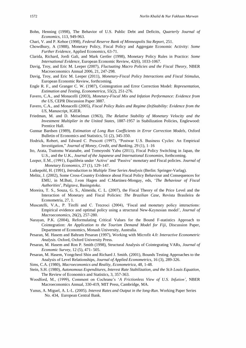
unity. The policy is „active‟ if coefficient of inflation rate is greater than zero and vice versa. Table 1

and 2 report the estimation results by using maximum likelihood estimation (MLE) for both monetary

and fiscal respectively.

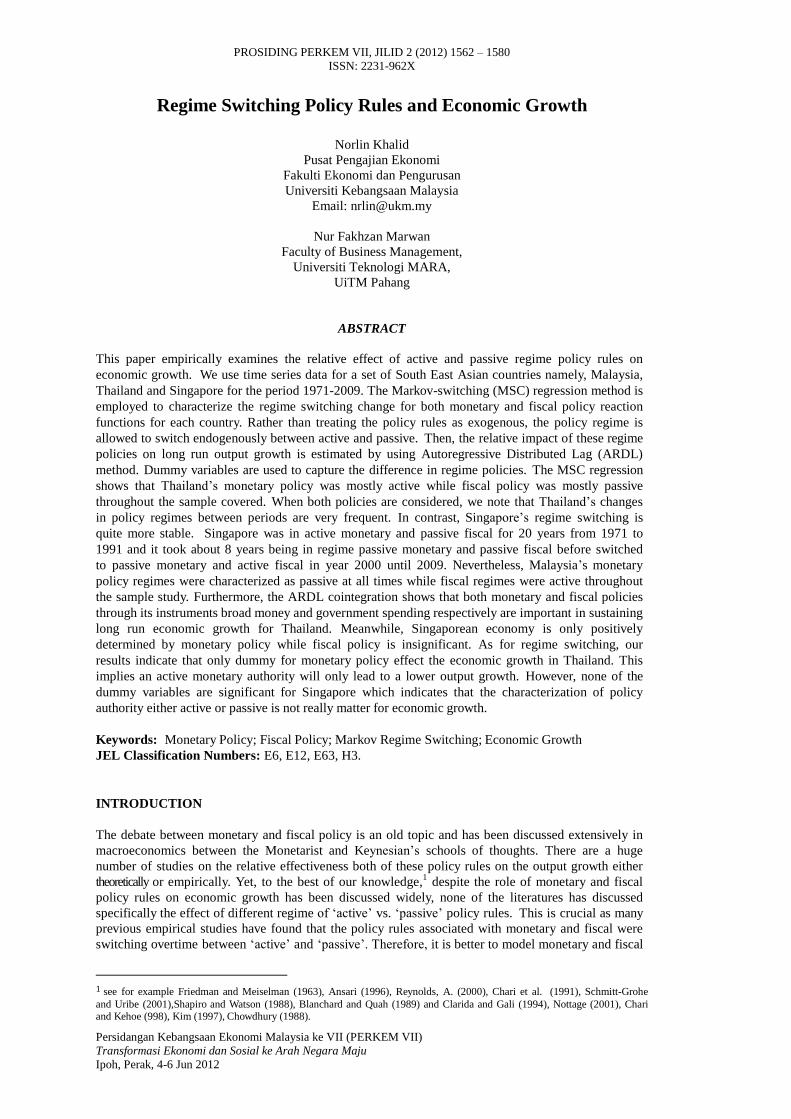
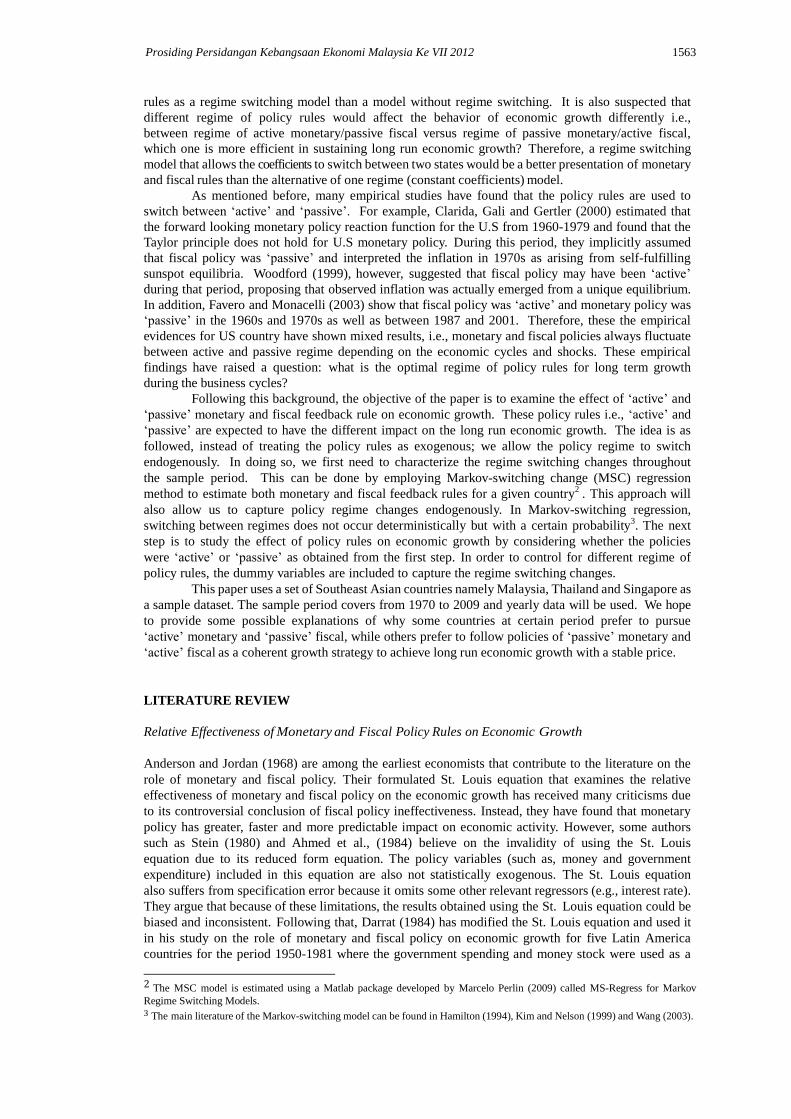
It is interesting to notice that, Thailand‟s monetary policy was mostly active while its fiscal

policy was mostly passive throughout the sample of the study. This can be seen in Figure 1 and 4 for

monetary and fiscal respectively. When both policies are considered, the monetary and fiscal regimes

were found to fluctuate between active and passive over time (see Table 3). As the result, the changes in

policy regimes between periods are very frequently. In contrast, Singapore‟s regime switching is more

stable as it did not show changing in regime policy rules very frequently. In terms of timing of regime

changes, Singapore was in Regime AM/PF for 20 years from 1971 to 1991 and it took about eight years

being in regime PM/PF before switched to regime PM/AF in year 2000 until 2009. On the other hand,

the results for Malaysian economy are totally different from Thailand and Singapore. Malaysia‟s

monetary policy regimes were characterized as passive at all times while fiscal regimes were active at

all times.


We examine the implication of policy rules on long run economic growth by taking into

account the policy regime switching obtained in the previous part. To capture the regime switching

active and passive, the dummy variables will be used which are labeled as DF and DM for fiscal and

monetary respectively. Notice that, the long run analysis for policy regime switching can only be done

for Thailand and Singapore given that their policy rules were switching throughout the sample of the

study. However with regard to Malaysia‟s policy rules, we found that the dummy policy variables are

time in varying since monetary policy was only active and fiscal policy was only passive over the

sample period of study. Therefore, long run implication of regime switching policy rules on output

growth cannot be analyzed for the case of Malaysia as this will result in perfect multicollinearity.

Using an ARDL approach, equation (3) is estimated to examine the relative effectiveness of

policy rules on economic growth. However, we first test for the existence of long run relationship

between the series of the variables. Table 4 provides the results of the F-statistics for each country to

various lag orders. The critical value is also reported in Table 4 based on the critical value suggested by

Narayan (2004) for a small sample size between 30 and 80. As can be seen from the table, the test

outcome of the significance levels for the long run relationship varies with the choice of lag-length. For

Thailand, the computed F-statistics are significant at least at 0.95 levels when the order of lags is 3,

while the F-statistics for Singapore is significance at least at 0.95 and 0.99 when the lag order is 3 and

4 respectively. This implies that the null hypothesis of no cointegration is rejected and therefore

there is a cointegration relationship among the variables. In this case, the ECM version of the ARDL

model is an efficient way in determining the long run relationship among the variables. Consequently,

there is a tendency for the variables to move together towards a long-run equilibrium. However, no

cointegration is found for the case of Malaysia for entire lag orders used in this study. This finding

implies that there is no long run relationship between the policy rules and economic growth for the case

of Malaysia.

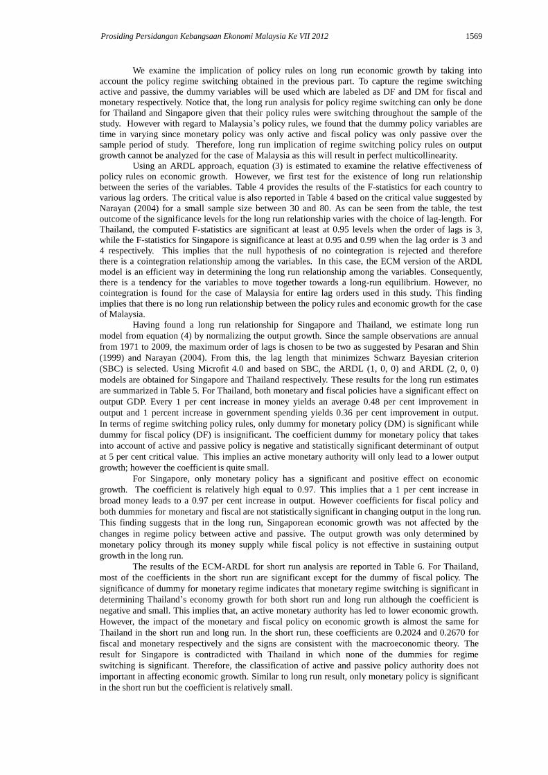
Having found a long run relationship for Singapore and Thailand, we estimate long run

model from equation (4) by normalizing the output growth. Since the sample observations are annual

from 1971 to 2009, the maximum order of lags is chosen to be two as suggested by Pesaran and Shin

(1999) and Narayan (2004). From this, the lag length that minimizes Schwarz Bayesian criterion

(SBC) is selected. Using Microfit 4.0 and based on SBC, the ARDL (1, 0, 0) and ARDL (2, 0, 0)

models are obtained for Singapore and Thailand respectively. These results for the long run estimates

are summarized in Table 5. For Thailand, both monetary and fiscal policies have a significant effect on

output GDP. Every 1 per cent increase in money yields an average 0.48 per cent improvement in

output and 1 percent increase in government spending yields 0.36 per cent improvement in output.

In terms of regime switching policy rules, only dummy for monetary policy (DM) is significant while

dummy for fiscal policy (DF) is insignificant. The coefficient dummy for monetary policy that takes

into account of active and passive policy is negative and statistically significant determinant of output

at 5 per cent critical value. This implies an active monetary authority will only lead to a lower output

growth; however the coefficient is quite small.

For Singapore, only monetary policy has a significant and positive effect on economic

growth. The coefficient is relatively high equal to 0.97. This implies that a 1 per cent increase in

broad money leads to a 0.97 per cent increase in output. However coefficients for fiscal policy and

both dummies for monetary and fiscal are not statistically significant in changing output in the long run.

This finding suggests that in the long run, Singaporean economic growth was not affected by the

changes in regime policy between active and passive. The output growth was only determined by

monetary policy through its money supply while fiscal policy is not effective in sustaining output

growth in the long run.

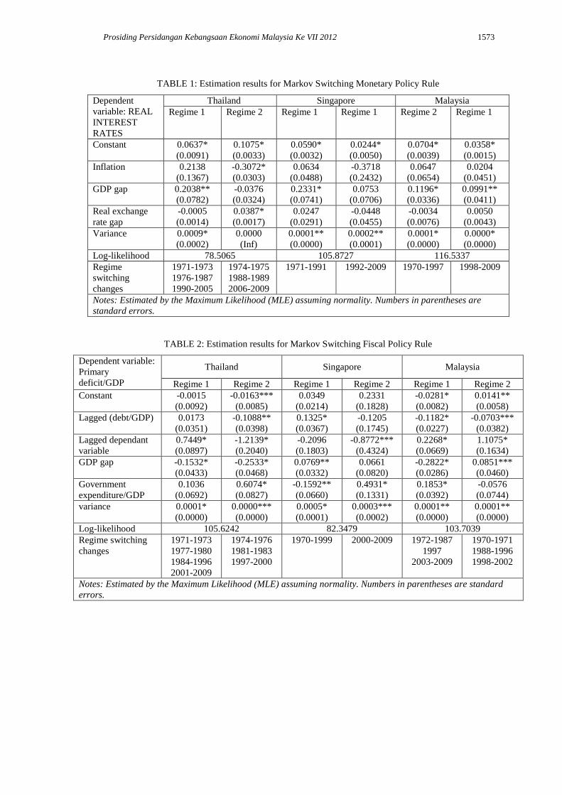
The results of the ECM-ARDL for short run analysis are reported in Table 6. For Thailand,

most of the coefficients in the short run are significant except for the dummy of fiscal policy. The

significance of dummy for monetary regime indicates that monetary regime switching is significant in

determining Thailand‟s economy growth for both short run and long run although the coefficient is

negative and small. This implies that, an active monetary authority has led to lower economic growth.

However, the impact of the monetary and fiscal policy on economic growth is almost the same for

Thailand in the short run and long run. In the short run, these coefficients are 0.2024 and 0.2670 for

fiscal and monetary respectively and the signs are consistent with the macroeconomic theory. The

result for Singapore is contradicted with Thailand in which none of the dummies for regime

switching is significant. Therefore, the classification of active and passive policy authority does not

important in affecting economic growth. Similar to long run result, only monetary policy is significant

in the short run but the coefficient is relatively small.


As shown by Table 6, the error correction terms (ECTt-1) for both countries are significant and

have the negative sign. Specifically, the estimated values of ECT are equal to -0.5555 and -0.3061 for

Thailand and Singapore respectively. In other words, the significant of ECT suggests that more than

55 and 31 percent of disequilibrium caused by previous years shock will be corrected in the current

year and converges back to long run equilibrium for Thailand and Singapore respectively. This

findings show that the speed of adjustment is really high especially for Thailand.

We apply a number of diagnostic tests to the ECM in order to check for the robustness of the

model. From the table we can see that both model for Thailand and Singapore have no evidence of

serial correlation and heteroskedasticity effect in the disturbances. Both models also pass the Jarque-

Bera normality test which suggests that the errors are normally distributed. By using Ramsey Resets

test for functional form we find Thailand‟s model specification is well specified whereas Singapore

has a problem of functional form. However, this is not crucial as the model is believed to be an

accurate form of policy specification from economic theory perspective in this study.

Derived from an estimated VAR, the variance decompositions (VDC) and impulse response

functions (IRF) are estimated that serve as tools for evaluating the dynamic interactions and strength of

causal relations among variables in the system. It should be noted that the VAR innovations may be

contemporaneously correlated. In other words, a shock in one variable may work through the

contemporaneous correlation with innovations in other variables. Thus, the responses of a variable to

innovations in another variable of interest cannot be adequately represented since isolated shocks to

individual variables cannot be identified due to contemporaneous correlation (Lutkepohl, 1991). As a

result, the Cholesky factorization that orthogonalizes the innovations is used as suggested by Sims

(1980) to solve the identification problem. The idea is to prespecify causal ordering of the variables. It

is because the results from VDC and IRF may be sensitive to the variables‟ ordering if the error terms‟

contemporaneous correlations are high. According to Sims (1980), the ordering of variables is

started with the most exogenous variables in the system and ended by the most endogenous variable.

To see whether the ordering could be a problem, we check the contemporaneous

correlations of VAR error terms. This can be seen in Table 7 and 8 for Singapore and Thailand

respectively. The results for Singapore show that there are very low correlations between the errors

terms as mostly are less than 0.2. This implies that for the case of Singapore, the result of IRF and

VDC are not sensitive to the variables‟ ordering. However, to perform VDC and IRF we arrange the

variables according to the following order, LNY, LNM and LNG. Similarly, the VAR errors terms for

Thailand are generally low but relatively, the correlations are quite high between LNY and LNG and

between LNG and LNM. Based on this, we arrange the ordering of the variables to the order LNG,

LNY and LNM for the case of Thailand.

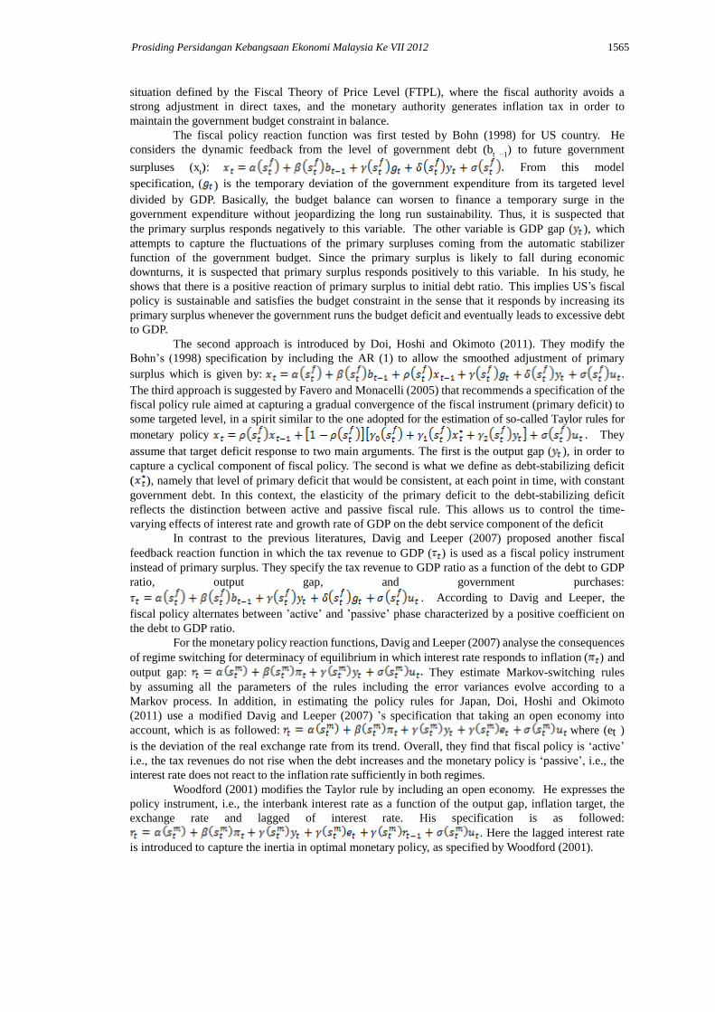
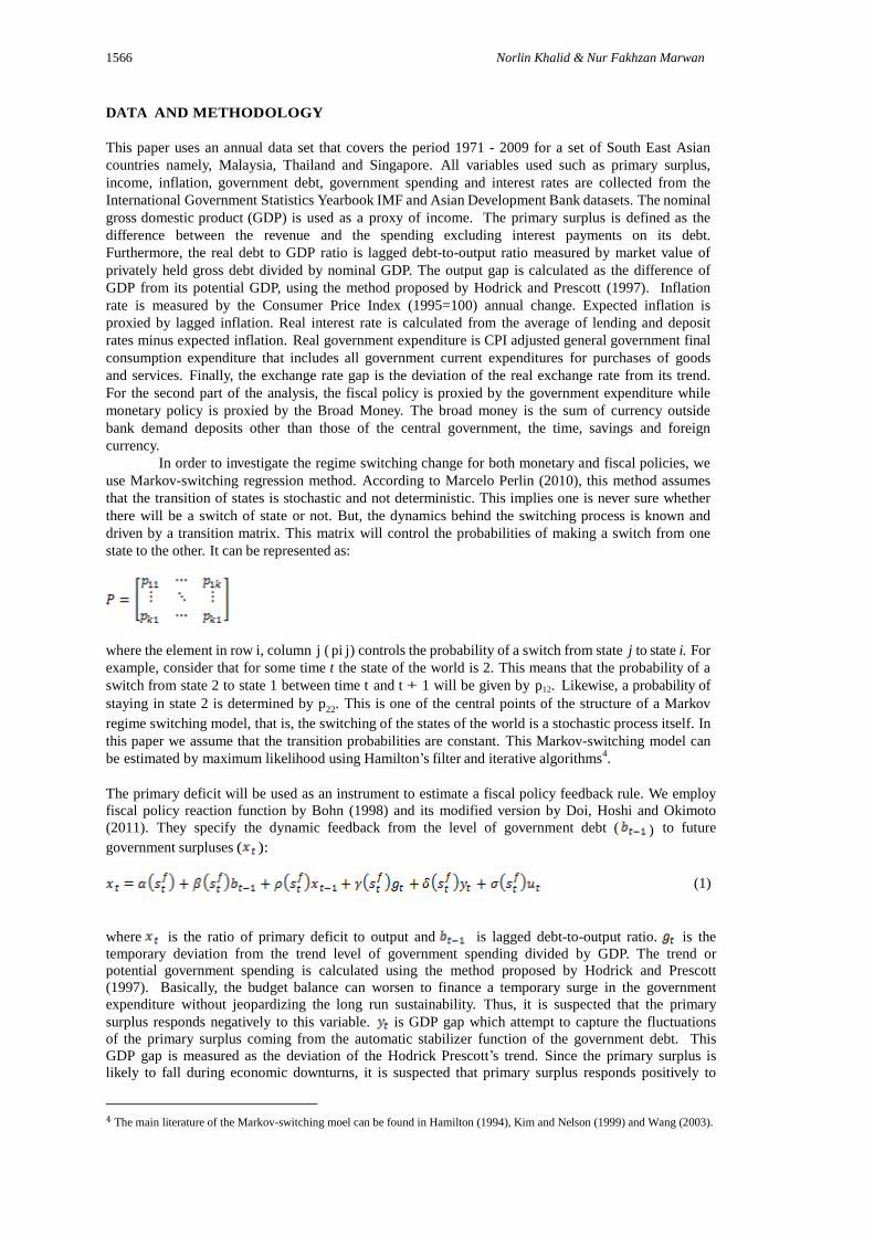
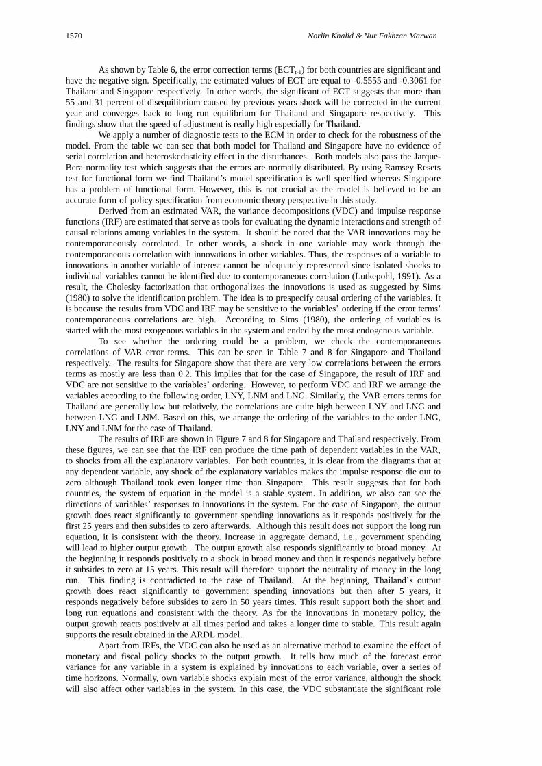
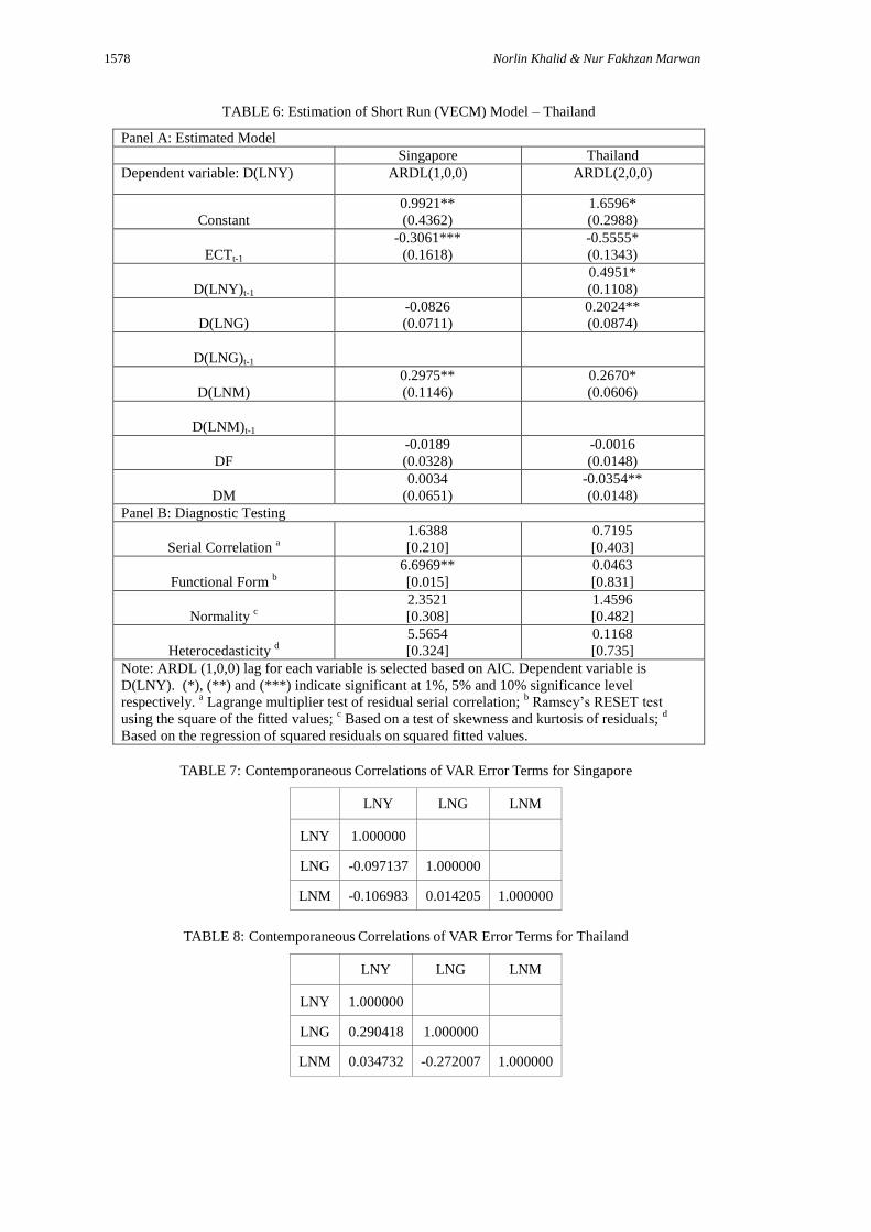
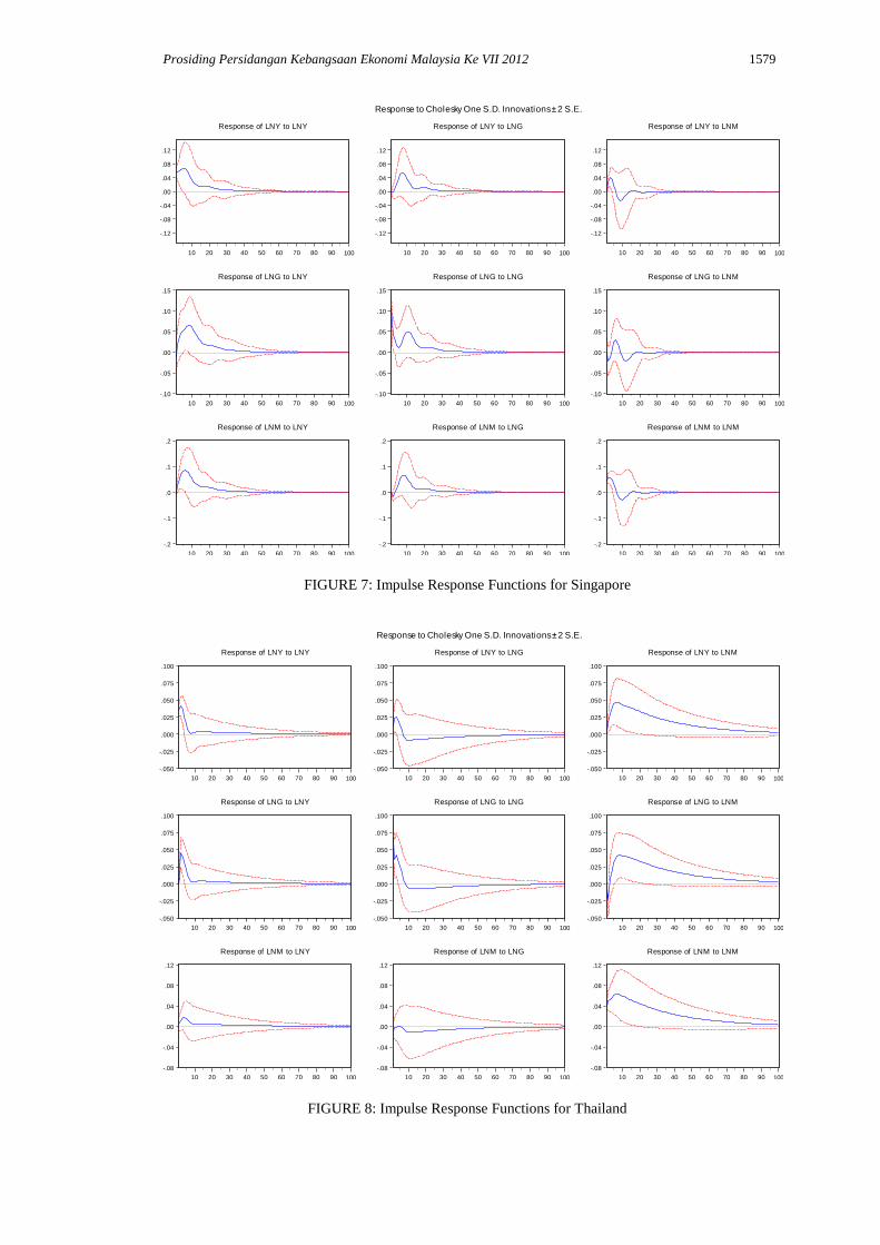
The results of IRF are shown in Figure 7 and 8 for Singapore and Thailand respectively. From

these figures, we can see that the IRF can produce the time path of dependent variables in the VAR,

to shocks from all the explanatory variables. For both countries, it is clear from the diagrams that at

any dependent variable, any shock of the explanatory variables makes the impulse response die out to

zero although Thailand took even longer time than Singapore. This result suggests that for both

countries, the system of equation in the model is a stable system. In addition, we also can see the

directions of variables‟ responses to innovations in the system. For the case of Singapore, the output

growth does react significantly to government spending innovations as it responds positively for the

first 25 years and then subsides to zero afterwards. Although this result does not support the long run

equation, it is consistent with the theory. Increase in aggregate demand, i.e., government spending

will lead to higher output growth. The output growth also responds significantly to broad money. At

the beginning it responds positively to a shock in broad money and then it responds negatively before

it subsides to zero at 15 years. This result will therefore support the neutrality of money in the long

run. This finding is contradicted to the case of Thailand. At the beginning, Thailand‟s output

growth does react significantly to government spending innovations but then after 5 years, it

responds negatively before subsides to zero in 50 years times. This result support both the short and

long run equations and consistent with the theory. As for the innovations in monetary policy, the

output growth reacts positively at all times period and takes a longer time to stable. This result again

supports the result obtained in the ARDL model.

Apart from IRFs, the VDC can also be used as an alternative method to examine the effect of

monetary and fiscal policy shocks to the output growth. It tells how much of the forecast error

variance for any variable in a system is explained by innovations to each variable, over a series of

time horizons. Normally, own variable shocks explain most of the error variance, although the shock

will also affect other variables in the system. In this case, the VDC substantiate the significant role


played by LNG and LNM in accounting for fluctuations in county‟s GDP growth (LNY). Initially, at 1-

year horizon, most of the Thailand‟s LNY forecast error variance attributable to variations in its own

shock and LNG with 91.5% and 8.43% respectively. However, the explanatory power of all variables

namely LNG and LNM increase at 3-year horizon in which the percentage of output growth forecast

variance explained by innovations in LNM is higher than explained by LNG. This result supports the

earlier findings that monetary policy (LNM) has a significant role in sustaining output growth while

fiscal policy (LNG) has an insignificant role in determining the output growth for Thailand.

For Singapore, at 1-year horizon, all forecast error variance in LNY is explained by its own

innovations with 100%. However, as we move further to 3 and 5-year horizon, the innovations in

LNM has increased dramatically to 19.7% and 16.4% respectively. In 5-year horizon, only 7.2%

innovation in LNY is explained by LNG. Therefore, this result again supports the finding for ARDL

model. However, after 5-year horizon, as can be seen from the Table, the percentage of forecast error

variance in LNY explained by LNG is higher than LNM. This implies, monetary policy has greater

impact on output growth for the first 5 years but not afterward.

CONCLUSION

Monetary and fiscal policies are always switching overtime between regime of active and passive in

order to counter the effect of inflation and depression as well as to achieve economic growth.

Therefore, a regime switching model that allows the coefficient to shift between two states would be a

better presentation of monetary and fiscal rules than the alternative of one regime (constant

coefficients) model. In this study, we work in an environment in which both monetary and fiscal

policy rules evolve according to a Markov process and investigate how this environment can affect the

long run economic growth. This paper uses the annual data of Malaysia, Thailand and Singapore for

the period 1971-2009 for the objective of assessing the effectiveness of different regime of „active‟ vs.

„passive‟ monetary and fiscal feedback rule in achieving long run economic growth. Using the

Markov-switching (MSC) regression, we find that Thailand‟s monetary policy was mostly active

while fiscal policy was mostly passive throughout the sample covered. When both policies are

considered, we note that Thailand‟s changes in policy regimes between periods are very frequent. In

contrast, Singapore‟s regime switching is quite more stable. Singapore was in active monetary and

passive fiscal regime for 20 years from 1971 to 1991 and it took about 8 years being in regime

passive monetary and passive fiscal before switched to passive monetary and active fiscal in year

2000 until 2009. Nevertheless, Malaysia‟s monetary policy regimes were characterized as passive at

all times while fiscal regimes were active throughout the sample study. Given these results, the

relative effectiveness of these regime policies on long run output growth is examined by using

autoregressive distributed lag (ARDL) model. For the case of Thailand, both monetary and fiscal

policies through its instrument broad money and government spending are important to sustain its

long run economic growth. For Singaporean case, on the other hand, findings show that only

monetary policy affects its long run growth. Results for the regime switching shows that only

dummy for monetary authority is significant for Thailand, indicates that an active monetary policy will

only lead to a lower output growth. Nevertheless, in the case of Singapore, none of the dummy

variables are significant, which implies that the characterization of policy authority either active or

passive is not important in its growth strategy. For Malaysia, as its monetary regime were passive and

fiscal regime were active all the time, the long run implication of regime switching policy rules on

output growth cannot be analyzed.

REFERENCES

Ahmed, et al. (1984), St. Louis Equation Restrictions and Criticisms Revisited, Journal of Money,

Credit and Banking, 16, 514-520.

Anderson, L. and J. Jordan (1968), Monetary and Fiscal Actions: A Test of Their Relative Importance

in Economic Stabilization, Federal Reserve Bank of St. Louis Review, 11-24.

Ansari, M.I (1996), Monetary vs. Fiscal Policy: Some Evidence from Vector Autoregression for India,

Journal of Asian Economics, 677-687.

Banerjee et. al (1993), Cointegration, Error Correction and the Econometric Analysis of Non-

Stationary Data, Oxford, Oxford University Press.


Bohn, Henning (1998), The Behavior of U.S. Public Debt and Deficits, Quarterly Journal of

Economics, 113, 949-963.

Chari, V. and P. Kehoe (1998), Federal Reserve Bank of Minneapolis Sta Report, 251.

Chowdhury, A (1988), Monetary Policy, Fiscal Policy and Aggregate Economic Activity: Some

Further Evidence, Applied Economics, 63-71.

Clarida, Richard, Jordi Gali, and Mark Gertler (1998), Monetary Policy Rules in Practice: Some

International Evidence, European Economic Review, 42(6), 1033-1067.

Davig, Troy, and Eric M. Leeper (2007), Fluctuating Macro Policies and the Fiscal Theory, NBER

Macroeconomics Annual 2006, 21, 247-298.

Davig, Troy, and Eric M. Leeper (2011), Monetary-Fiscal Policy Interactions and Fiscal Stimulus,

European Economic Review, forthcoming.

Engle R. F., and Granger C. W. (1987), Cointegration and Error Correction Model: Representation,

Estimation and Testing, Econometrica, 55(2), 251-276.

Favero, C.A., and Monacelli (2003), Monetary-Fiscal Mix and Infation Performance: Evidence from

the US, CEPR Discussion Paper 3887.

Favero, C.A., and Monacelli (2005), Fiscal Policy Rules and Regime (In)Stability: Evidence from the

US, Manuscript, IGIER.

Friedman, M. and D. Meiselman (1963), The Relative Stability of Monetary Velocity and the

Investment Multiplier in the United States, 1887-1957 in Stabilization Policies, Englewood:

Prentice Hall.

Gunnar Bardsen (1989), Estimation of Long Run Coefficients in Error Correction Models, Oxford

Bulletin of Economics and Statistics, 51 (2), 345-350.

Hodrick, Robert, and Edward C. Prescott (1997), “Postwar U.S. Business Cycles: An Empirical

Investigation,” Journal of Money, Credit, and Banking, 29 (1), 1–16

Ito, Arata, Tsutomu Watanabe, and Tomoyoshi Yabu (2011), Fiscal Policy Switching in Japan, the

U.S., and the U.K., Journal of the Japanese and International Economies, forthcoming.

Leeper, E.M., (1991), Equilibria under „Active‟ and „Passive‟ monetary and Fiscal policies. Journal of

Monetary Economics, 27 (1), 129–147.

Lutkepohl, H. (1991), Introduction to Multiple Time Series Analysis (Berlin: Springer-Varlag).

Melitz, J. (2002), Some Cross-Country Evidence about Fiscal Policy Behaviour and Consequences for

EMU, in M.Buti, J.von Hagen and C.Martinez-Mongay, eds, „The Behaviour of Fiscal

Authorities‟, Palgrave, Basingstoke.

Moreira, T. S., Souza, G. S., Almeida, C. L. (2007), the Fiscal Theory of the Price Level and the

Interaction of Monetary and Fiscal Policies: The Brazilian Case, Revista Brasileira de

Econometria, 27, 1.

Muscatelli, V.A., P. Tirelli and C. Trecroci (2004), „Fiscal and monetary policy interactions:

Empirical evidence and optimal policy using a structural New-Keynesian model‟, Journal of

Macroeconomics, 26(2), 257-280.

Narayan, P.K. (2004), Reformulating Critical Values for the Bound F-statistics Approach to

Cointegration: An Application to the Tourism Demand Model for Fiji, Discussion Paper,

Department of Economics, Monash University, Australia.

Pesaran, M. Hasem and Bahram Pesaran (1997), Working with Microfit 4.0: Interactive Econometric

Analysis. Oxford, Oxford University Press.

Pesaran, M. Hasem and Ron P. Smith (1998), Structural Analysis of Cointegrating VARs, Journal of

Economic Survey, 12 (5), 471- 505.

Pesaran, M. Hasem, Yongcheol Shin and Richard J. Smith. (2001), Bounds Testing Approaches to the

Analysis of Level Relationships, Journal of Applied Econometrics, 16 (3), 289-326.

Sims, C.A. (1980), Macroeconomics and Reality, Econometrica, 48, 1-48.

Stein, S.H. (1980), Autonomous Expenditures, Interest Rate Stabilization, and the St.h Louis Equation,

The Review of Economics and Statistics, 3, 357-363.

Woodford, M., (1999), Comment on Cochrane‟s „A Frictionless View of U.S. Infation’, NBER

Macroeconomics Annual, 330-419, MIT Press, Cambridge, MA.

Yunus, A. Miguel, A. L-L. (2005). Interest Rates and Output in the long-Run. Working Paper Series

No. 434, European Central Bank.


TABLE 1: Estimation results for Markov Switching Monetary Policy Rule

Dependent

variable: REAL

INTEREST

RATES

Thailand Singapore Malaysia

Regime 1 Regime 2 Regime 1 Regime 1 Regime 2 Regime 1

Constant 0.0637*

(0.0091)

0.1075*

(0.0033)

0.0590*

(0.0032)

0.0244*

(0.0050)

0.0704*

(0.0039)

0.0358*

(0.0015)

Inflation

0.2138

(0.1367)

-0.3072*

(0.0303)

0.0634

(0.0488)

-0.3718

(0.2432)

0.0647

(0.0654)

0.0204

(0.0451)

GDP gap

0.2038**

(0.0782)

-0.0376

(0.0324)

0.2331*

(0.0741)

0.0753

(0.0706)

0.1196*

(0.0336)

0.0991**

(0.0411)

Real exchange

rate gap

-0.0005

(0.0014)

0.0387*

(0.0017)

0.0247

(0.0291)

-0.0448

(0.0455)

-0.0034

(0.0076)

0.0050

(0.0043)

Variance 0.0009*

(0.0002)

0.0000

(Inf)

0.0001**

(0.0000)

0.0002**

(0.0001)

0.0001*

(0.0000)

0.0000*

(0.0000)

Log-likelihood 78.5065 105.8727 116.5337

Regime

switching

changes

1971-1973

1976-1987

1990-2005

1974-1975

1988-1989

2006-2009

1971-1991 1992-2009 1970-1997 1998-2009

Notes: Estimated by the Maximum Likelihood (MLE) assuming normality. Numbers in parentheses are

standard errors.

TABLE 2: Estimation results for Markov Switching Fiscal Policy Rule

Dependent variable:

Primary

deficit/GDP


Regime 1 Regime 2 Regime 1 Regime 2 Regime 1 Regime 2

Constant -0.0015

(0.0092)

-0.0163***

(0.0085)

0.0349

(0.0214)

0.2331

(0.1828)

-0.0281*

(0.0082)

0.0141**

(0.0058)

Lagged (debt/GDP) 0.0173

(0.0351)

-0.1088**

(0.0398)

0.1325*

(0.0367)

-0.1205

(0.1745)

-0.1182*

(0.0227)

-0.0703***

(0.0382)

Lagged dependant

variable

0.7449*

(0.0897)

-1.2139*

(0.2040)

-0.2096

(0.1803)

-0.8772***

(0.4324)

0.2268*

(0.0669)

1.1075*

(0.1634)

GDP gap -0.1532*

(0.0433)

-0.2533*

(0.0468)

0.0769**

(0.0332)

0.0661

(0.0820)

-0.2822*

(0.0286)

0.0851***

(0.0460)

Government

expenditure/GDP

0.1036

(0.0692)

0.6074*

(0.0827)

-0.1592**

(0.0660)

0.4931*

(0.1331)

0.1853*

(0.0392)

-0.0576

(0.0744)

variance 0.0001*

(0.0000)

0.0000***

(0.0000)

0.0005*

(0.0001)

0.0003***

(0.0002)

0.0001**

(0.0000)

0.0001**

(0.0000)

Log-likelihood 105.6242 82.3479 103.7039

Regime switching

changes

1971-1973

1977-1980

1984-1996

2001-2009

1974-1976

1981-1983

1997-2000

1970-1999 2000-2009 1972-1987

1997

2003-2009

1970-1971

1988-1996

1998-2002

Notes: Estimated by the Maximum Likelihood (MLE) assuming normality. Numbers in parentheses are standard

errors.


1970 1975 1980 1985 1990 1995 2000 2005 20090

0.1

0.2

0.3

0.4

0.5

0.6

0.7

0.8

0.9

1

Time

Sm

ooth

ed S

tate

s P

robabili

ties

Regime 1

Regime 2

FIGURE 1: Thailand‟s Probability of Regime 1 (Active) and Regime 2 (Passive) in a Two-Regime

MRS Estimation of the Monetary Policy Rule

1970 1975 1980 1985 1990 1995 2000 2005 2009-0.2

0

0.2

0.4

0.6

0.8

1

1.2

Time

Sm

ooth

ed S

tate

s P

robabili

ties

Regime 1

Regime 2

FIGURE 2: Singapore‟s Probability of Regime 1 (Active) and Regime 2 (Passive) in a Two-Regime


1970 1975 1980 1985 1990 1995 2000 2005 20090

0.1

0.2

0.3

0.4

0.5

0.6

0.7

0.8

0.9

1

Time

Sm

ooth

ed S

tate

s P

robabili

ties

State 1

Regime 2

FIGURE 3: Malaysia‟s Probability of Regime 1 (Passive) and Regime 2 (Passive) in a Two-Regime



1970 1975 1980 1985 1990 1995 2000 2005 20090

0.2

0.4

0.6

0.8

1

1.2

1.4

Time

Sm

ooth

ed S

tate

s P

robabili

ties

Regime 1

Regime 2

FIGURE 4: Thailand‟s Probability of Regime 1 (Passive) and Regime 2 (Active) in a Two-Regime

MRS Estimation of the Fiscal Policy Rule

1970 1975 1980 1985 1990 1995 2000 2005 20090

0.2

0.4

0.6

0.8

1

Time

Sm

ooth

ed S

tate

s P

robabili

ties

Regime 1

Regime 2

FIGURE 5: Singapore‟s Probability of Regime 1 (Passive) and Regime 2 (Active) in a Two-Regime


1970 1975 1980 1985 1990 1995 2000 2005 20090

0.2

0.4

0.6

0.8

1

1.2

1.4

Time

Sm

ooth

ed S

tate

s P

robabili

ties

Regime 1

State 2

FIGURE 6: Malaysia‟s Probability of Regime 1 (Active) and Regime 2 (Active) in a Two-Regime



TABLE 3: Classification of Regime Policy Rules for both Monetary and Fiscal.


1971 1 1 2 Note:

1972 1 1 2 Regime 1 - Active Monetary/Passive Fiscal

1973 1 1 2 Regime 2 - Passive Monetary/Active Fiscal

1974 2 1 2 Regime 3 - Active Monetary/Active Fiscal

1975 2 1 2 Regime 4 - Passive Monetary/Passive Fiscal

1976 3 1 2

1977 1 1 2

1978 1 1 2

1979 1 1 2

1980 1 1 2

1981 3 1 2

1982 3 1 2

1983 3 1 2

1984 1 1 2

1985 1 1 2

1986 1 1 2

1987 1 1 2

1988 4 1 2

1989 4 1 2

1990 1 1 2

1991 1 1 2

1992 1 4 2

1993 1 4 2

1994 1 4 2

1995 1 4 2

1996 1 4 2

1997 3 4 2

1998 3 4 2

1999 3 4 2

2000 3 2 2

2001 1 2 2

2002 1 2 2

2003 1 2 2

2004 1 2 2

2005 1 2 2

2006 4 2 2

2007 4 2 2

2008 4 2 2

2009 4 2 2


TABLE 4: F-statistics for Testing the Existence of a Long run Equation

Countries F- statistics Lag

Significance

Level

Bound Critical Values*

(restricted intercept and no

trend)

I(0) I(1)

Malaysia 1.7727 2

1 % 4.030 5.463 Thailand 3.1453 2

Singapore 3.2685 2

Malaysia 1.4799 3

5 % 2.928 4.042 Thailand 4.6585** 3

Singapore 4.8254** 3

Malaysia 3.1161 4

10 % 2.458 3.432 Thailand 2.9151 4

Singapore 6.4994* 4

Note: * Based on Narayan (2004)

TABLE 5: Estimation of Long Run Coefficients

Country/

ARDL(p,q,r)

Singapore

ARDL(1,0,0)

Thailand

ARDL(2,0,0)

Dependent variable: LNY

Constant 3.2409*

(0.8461) 2.9879*

(0.2831)

LNG -0.2699

(0.3292)

0.3644*

(0.0942)

LNM 0.9717*

(0.2768)

0.4807*

(0.0706)

DF -0.0619

(0.1086)

-0.0029

(0.0268)

DM 0.0110

(0.1713)

-0.0637**

(0.0277)

Note: (*), (**) and (***) indicate significant at 1%, 5% and 10% significance level respectively.

Numbers in parentheses are standard errors.


TABLE 6: Estimation of Short Run (VECM) Model – Thailand

Panel A: Estimated Model

Singapore Thailand

Dependent variable: D(LNY) ARDL(1,0,0) ARDL(2,0,0)

Constant

0.9921**

(0.4362)

1.6596*

(0.2988)

ECTt-1

-0.3061***

(0.1618)

-0.5555*

(0.1343)

D(LNY)t-1

0.4951*

(0.1108)

D(LNG)

-0.0826

(0.0711)

0.2024**

(0.0874)

D(LNG)t-1

D(LNM)

0.2975**

(0.1146)

0.2670*

(0.0606)

D(LNM)t-1

DF

-0.0189

(0.0328)

-0.0016

(0.0148)

DM

0.0034

(0.0651)

-0.0354**

(0.0148)

Panel B: Diagnostic Testing

Serial Correlation a

1.6388

[0.210]

0.7195

[0.403]

Functional Form b

6.6969**

[0.015]

0.0463

[0.831]

Normality c

2.3521

[0.308]

1.4596

[0.482]

Heterocedasticity d

5.5654

[0.324]

0.1168

[0.735]

Note: ARDL (1,0,0) lag for each variable is selected based on AIC. Dependent variable is

D(LNY). (*), (**) and (***) indicate significant at 1%, 5% and 10% significance level

respectively. a Lagrange multiplier test of residual serial correlation;

b Ramsey‟s RESET test

using the square of the fitted values; c Based on a test of skewness and kurtosis of residuals;

d

Based on the regression of squared residuals on squared fitted values.

TABLE 7: Contemporaneous Correlations of VAR Error Terms for Singapore

LNY LNG LNM

LNY

1.000000

LNG -0.097137 1.000000

LNM -0.106983 0.014205 1.000000

TABLE 8: Contemporaneous Correlations of VAR Error Terms for Thailand

LNY LNG LNM

LNY

1.000000

LNG 0.290418 1.000000

LNM 0.034732 -0.272007 1.000000


-.12

-.08

-.04

.00

.04

.08

.12

10 20 30 40 50 60 70 80 90 100

Response of LNY to LNY

-.12

-.08

-.04

.00

.04

.08

.12

10 20 30 40 50 60 70 80 90 100

Response of LNY to LNG

-.12

-.08

-.04

.00

.04

.08

.12

10 20 30 40 50 60 70 80 90 100

Response of LNY to LNM

-.10

-.05

.00

.05

.10

.15

10 20 30 40 50 60 70 80 90 100

Response of LNG to LNY

-.10

-.05

.00

.05

.10

.15

10 20 30 40 50 60 70 80 90 100

Response of LNG to LNG

-.10

-.05

.00

.05

.10

.15

10 20 30 40 50 60 70 80 90 100

Response of LNG to LNM

-.2

-.1

.0

.1

.2

10 20 30 40 50 60 70 80 90 100

Response of LNM to LNY

-.2

-.1

.0

.1

.2

10 20 30 40 50 60 70 80 90 100

Response of LNM to LNG

-.2

-.1

.0

.1

.2

10 20 30 40 50 60 70 80 90 100

Response of LNM to LNM

Response to Cholesky One S.D. Innovations ± 2 S.E.

FIGURE 7: Impulse Response Functions for Singapore

-.050

-.025

.000

.025

.050

.075

.100

10 20 30 40 50 60 70 80 90 100

Response of LNY to LNY

-.050

-.025

.000

.025

.050

.075

.100

10 20 30 40 50 60 70 80 90 100

Response of LNY to LNG

-.050

-.025

.000

.025

.050

.075

.100

10 20 30 40 50 60 70 80 90 100

Response of LNY to LNM

-.050

-.025

.000

.025

.050

.075

.100

10 20 30 40 50 60 70 80 90 100

Response of LNG to LNY

-.050

-.025

.000

.025

.050

.075

.100

10 20 30 40 50 60 70 80 90 100

Response of LNG to LNG

-.050

-.025

.000

.025

.050

.075

.100

10 20 30 40 50 60 70 80 90 100

Response of LNG to LNM

-.08

-.04

.00

.04

.08

.12

10 20 30 40 50 60 70 80 90 100

Response of LNM to LNY

-.08

-.04

.00

.04

.08

.12

10 20 30 40 50 60 70 80 90 100

Response of LNM to LNG

-.08

-.04

.00

.04

.08

.12

10 20 30 40 50 60 70 80 90 100

Response of LNM to LNM

Response to Cholesky One S.D. Innovations ± 2 S.E.

FIGURE 8: Impulse Response Functions for Thailand


TABLE 9: Variance Decompositions - Thailand

Percentage of forecast variance explained by innovations in:

Period LNY LNG LNM

i) Variance Decomposition of LNY

1 91.56576 8.434241 0.000000

3 63.08823 19.54950 17.36228

5 43.32554 16.57955 40.09490

10 22.90830 9.637513 67.45419

15 16.87863 7.976608 75.14476

20 14.06871 7.240038 78.69125

ii) Variance Decomposition of LNG:

1 0.000000 100.0000 0.000000

3 29.85558 65.28322 4.861207

5 30.09324 57.98223 11.92454

10 20.63699 39.39597 39.96704

15 16.01117 30.73498 53.25384

20 13.59986 26.38646 60.01368

iii) Variance Decomposition of LNM:

1 1.412532 7.398787 91.18868

3 6.038370 1.734972 92.22666

5 7.052982 0.855017 92.09200

10 4.048460 1.247176 94.70436

15 3.044781 2.062753 94.89247

20 2.634553 2.414902 94.95054

TABLE 10: Variance Decompositions – Singapore

Percentage of forecast variance explained by innovations in:

Period LNY LNG LNM

i) Variance Decomposition of LNY

1 100.0000 0.000000 0.000000

3 80.11730 0.170470 19.71223

5 76.27482 7.248931 16.47625

10 62.63845 25.94556 11.41599

15 61.91810 26.59395 11.48795

20 62.12895 26.67260 11.19845

ii) Variance Decomposition of LNG:

1 0.943561 99.05497 0.001471

3 11.13755 85.16319 3.699259

5 28.93796 65.62668 5.435360

10 51.43009 42.64159 5.928318

15 50.88953 42.46809 6.642386

20 51.56993 41.97104 6.459027

iii) Variance Decomposition of LNM:

1 1.144527 0.000000 98.85547

3 27.32537 2.619336 70.05530

5 51.83531 6.088750 42.07594

10 55.05796 26.44274 18.49930

15 54.41861 27.88874 17.69264

20 54.98953 27.89423 17.11623

regime switching policy rules and economic growth the msc model is estimated using a matlab package...

Documents