refresher in statistics and analysis skill
TRANSCRIPT

Refresher in Statistics and Analysis Skills
Dr Santam Chakraborty

Statistics - A subject which most statisticians find difficult but in which nearly all physicians are expert.
- Stephen Senn, Statistical Issues in Drug Development

What you will find in this presentation● Only 1 calculation● Only 1 formula● Lots of Cartoons & Quotes !!!

Intro

Cartoon Number 731 xkcd.com by Randall Munroe

Data

Data Types
DataQualitative
dataQuantitative
Data
Nominal Data
Ordinal Data
Discrete Data
Continuous Data

Key Points
● Converting quantitative data to qualitative data is not advisable as it leads to data loss.
● QoL data is always qualitative but analyzed often as quantitative data
● Most medical researchers gather both qualitative & quantitative data but disregard qualitative data

Types of Measurements
BINARY NOMINAL ORDINAL
COUNT CONTINOUS

Variable Types
VariableResponse Variable
Non Response Variable
Independent Variable
Experimental Variable
Confounder Variable

Data Collection

Collecting Data
● This is the most neglected yet most vital part of the process.
● A structured way to collect data - Form● Data collection instruments :
○ Surveys
○ Interviews
○ Focus Groups
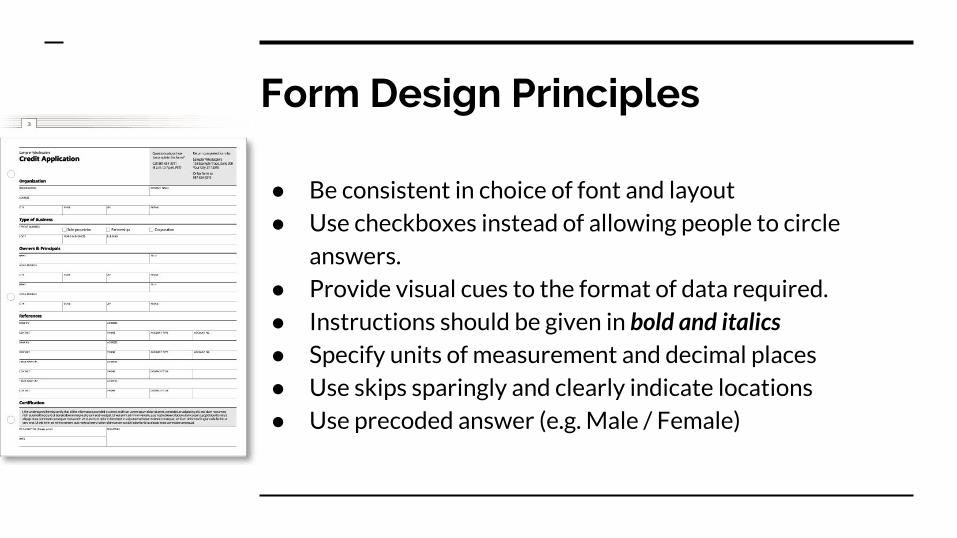
Form Design Principles
● Be consistent in choice of font and layout● Use checkboxes instead of allowing people to circle
answers.● Provide visual cues to the format of data required.● Instructions should be given in bold and italics● Specify units of measurement and decimal places● Use skips sparingly and clearly indicate locations ● Use precoded answer (e.g. Male / Female)


Resources
1. http://www.slideshare.net/psykoreactor/best-practices-for-form-design
2. https://www.lynda.com/Web-Interactive-User-Experience-tutorials/We
b-Form-Design-Best-Practices/83786-2.html?utm_medium=integrated-p
artnership&utm_source=slideshare
3. Bellary S, Krishnankutty B, Latha MS. Basics of case report form designing in clinical research. Perspect Clin Res. 2014 Oct;5(4):159–66.

Data Storage

Databases : Advantages
● Allow multi-user access● Respect data integrity● Allow data validation● Avoid data redundancy● Allow flexible and customized queries

Databases : Disadvantages
● More difficult to learn● May require an understanding of networking
related concepts● Software maintenance and updates are an issue. ● Have a clear idea of the information that needs to
be included. ● Form design is required.


Spreadsheet Tips
1. Header row should be in the first row only. Don't make fancy 2/3 row headers.
2. Set the locale to UK / India if you are planning to use DD/MM/YYYY as the date scheme
3. Freeze the first row and first column to ease data entry.4. Use conditional formatting to pick up mistakes while
doing data-entry.5. Avoid extensive code books - it is easier to recode data6. Use different sheets sparingly.

Spreadsheet Tips
1. Remember excel is not a relational database - so donot use the sort option.
2. If using the sort option select all the coloumns before using sort
3. If you use a formula during data entry make the cell protected or hidden to avoid inadvertent changes
4. Stick to a case “UPPERCASE” or “lowercase”.

SPSS Tips
1. Never forget to use variable labels. Setting this at design stage ensures that everyone remembers what is to be entered.
2. Value labels are your friend - dont use this sparingly.
3. Ensure that the data - type is chosen appropriately.
Resources
1. Disciplined use of spreadsheets for data entry : http://www.reading.ac.uk/ssc/resource-packs/ILRI_2006-Nov/GoodStatisticalPractice/publications/guides/topsde.html
2. Using an Excel data entry form : https://www.pryor.com/blog/ease-the-pain-of-data-entry-with-an-excel-forms-template/
3. SPSS data entry tips : https://www.youtube.com/watch?v=N-krh4EaELE

Data Analysis

A Statistical Analysis Plan (SAP) is the starting point of your analysis
Tip
If you are at a loss when it comes to writing your SAP write the paper results - it will help you to visualize the analysis plan.

Elements of a SAP
Define the research hypothesis
Define the end- points
Define the Statistical methods

Research Hypothesis
1. Derives from the research question2. Equally important for prospective or
retrospective studies. 3. Helps in choosing the correct endpoints for
the objectives appropriate to the hypothesis. 4. Often helps us to understand our underlying
motivation for the research

Research Question
A question that is designed to address a “perceived” gap in the current state of knowledge about a condition.
“I want to know how many new patients are seen by my colleague instead of me”
“I want to know how many patients survive for 5 years after coming to me”

PICO(T)
1. Population - To be defined for all studies2. Intervention - Essential if you want to study the
effect of an intervention3. Comparison Groups - Essential if you want to
define the benefit of an intervention4. Outcome - To be defined for all studies5. Time - Essential if a time to event endpoint is
chosen.

P New Patients presenting to my hospital
New Patients presenting to my Hospital
I Undergo a Consultation Treatment given by me
C Colleague or Me -
O Number of patients Survive their disease
(T) Over the last week Till 5 years
See other great examples of PICOs formulated from daily practice questions at PICO examples provided by the Cochrane Library : http://learntech.physiol.ox.ac.uk/cochrane_tutorial/cochlibd0e187.php

Always do a systematic review after formulating the PICO
Tip
The Cochrane Handbook is a great way to understand the systematic review process
http://training.cochrane.org/handbook

Alpha and Beta
1. Our research question is defined with the perspective of the population but we can rarely study that.
2. The value of an observation in a representative and random sample is considered to approximate the population value.
3. Repeated samples from the same population will likely yield different results for this value.
4. Alpha and Beta are measures of this uncertainty.

Researcher’s Decision
Reject Null Hypothesis Retain Null Hypothesis
Reality
Null Hypothesis is True
Type I Error (probability of this occurring = Alpha)
Correct
Null Hypothesis is False
Correct � Type II Error (Probability of this occurring is beta)


Resources
1. Hypothesis Testing and statistical Power : http://my.ilstu.edu/~wjschne/138/Psychology138Lab14.html (with beautiful animated gifs !!!)
2. Errors in Hypothesis Testing : http://www.psychstat.missouristate.edu/IntroBook3/sbk20.htm

Descriptive Stats

Before the Analysis
1. Ensure that you make a folder for the data file and take a backup
2. If analyzing in SPSS ensure that the SPSS viewer file is saved in the same folder
3. Ensure that the file version is correct if you have used multiple versions of the same file.
4. Turn off the distractions and turn on some light music.

Describe the data
Always start with descriptives
1. Frequencies for Qualitative Variables2. Mean and SD for Quantitative Variables. 3. Check for missing values 4. Check for outliers (graphs)

Measures of Central Tendency1. Mean : Heavily influenced by atypical values2. Median: Heavily influenced by ties. Median is
also not amenable to further calculation and rarely used in statistical procedures.
3. Mode : Also susceptible to ties. But the only type of central tendency for nominal data.
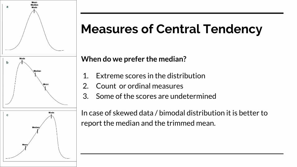
Measures of Central Tendency
When do we prefer the median?
1. Extreme scores in the distribution2. Count or ordinal measures3. Some of the scores are undetermined
In case of skewed data / bimodal distribution it is better to report the median and the trimmed mean.

Quantiles
● These are measures of variability as well as central tendency. Each quantile has the same number of observations.
● Median can be conceptualized as the 50% quantile● Tertile: Split by 33% (3 parts)● Quartile : Split by 25% (4 parts)● Quintile : Split by 20% (5 parts)● Decile : Split by 10% (10 parts)

Measures of Spread
● Range : Not useful when you have extreme values● Interquartile Range : Usually reported along with median
- range between 25th - 75th quartile● Standard deviation and Variance : Useful if the
distribution is symmetric● 95% confidence interval of mean technically is a
measure of how closely your sample mean approximates the “unknown” population mean. In case of normal distribution this corresponds to ±1.96 standard deviation

Box Plot : http://www.physics.csbsju.edu/stats/box2.html
Box Whisker Plots

Data Distribution
1. Binary / Nominal / Ordinal : Frequencies of categories
2. Continuous Variable:a. Histogram
b. Cumulative Histogram
c. Quantiles
d. Moments (measures of central tendency & skewness)
3. Skewed data : Nonparametric methods of analysis (i.e. methods that do not assume that the distribution is normal).

Density Plots & Histograms
Quick R: Histograms & Density Plots : http://www.statmethods.net/graphs/density.html

Spaghetti Plots

Bar Charts : Best Practices
1. Give the count if your Y axis is in percentages2. Start the Y axis from 03. Try to arrange categories by frequency4. Use a consistent color scheme - dont use different
colors in the bars unless they represent different categories.
5. Avoid stacked bar charts unless you want to show part to whole relationships
6. Space between bars = 1/2 of the bar width
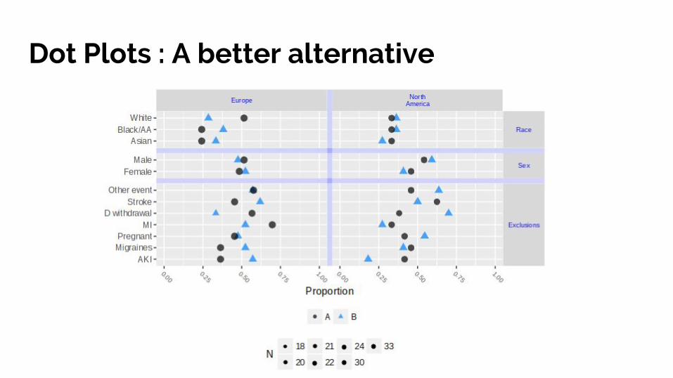
Dot Plots : A better alternative

Bivariate Associations
Missing Values
Missing Completely at Random (MCAR) : Missingness of a value is not
dependant on another variable (e.g. randomly patients forget to answer some
QOL items)
Missing at random (MAR) : Missingness of a value is dependant on another variable (e.g. patients presenting in late afternoon do not fill QOL forms)
Missing not at random (MNAR) : Missingness depends on a particular
characteristic inherent in the variable (e.g. only patients with poor QOL do not
fill QOL forms).

Missing Values
1. Deletion methods : In this some form of the data is deleted. Most common approach used in SPSS is listwise deletion. Alternative is pairwise deletion.
2. Single Imputation: Most common method is mean / median substitution. Alternatively dummy coding can be used especially if a categorical variable.
3. Model based Imputation : Multiple imputation and maximum likelihod based methods.

Missing Values
List wise Deletion Pairwise Deletion
Effect on Sample Size Reduced Mostly remains same
Effect on Power Reduced Mostly remains same
Simplicity Yes Yes
Model comparison Yes No
Bias if MCAR Yes Yes

Single Value Imputation with Mean / Median
Single Value Imputation with simple regression
Resources
1. How to diagnose the missing data mechanism: http://www.theanalysisfactor.com/missing-data-mechanism/
2. Missing data : Pairwise and Listwise Deletions which to use : http://www-01.ibm.com/support/docview.wss?uid=swg21475199
3. Missing data and how to deal with it ( A nice presentation) : https://liberalarts.utexas.edu/prc/_files/cs/Missing-Data.pdf

Inferential Stats

Inferential Statistics
1. Hypothesis Testing2. Comparing 2 proportions3. Non Parametric Statistical Tests4. Correlation5. Linear Models
Hypothesis testing
1. Formal testing if the null hypothesis is untrue i.e. disprove the null hypothesis
2. The null hypothesis is equivalent to a straw man - a sham argument set up to be defeated.
3. The type of “tail” depends on the nature of the alternate hypothesis
Failure to reject the null hypothesis is not the proof of it’s truth - in other words absence of evidence is not evidence of it’s absence

Hypothesis testing : Tails
● Bill gates is earning the same $$ per month as me - H
0
● Bill gates is earning less $$ per month than me - H
1 (one tailed)
● The $$ that Bill Gates earns is different from what I earn - H
1 (two tailed)

Classifications of “significant" or “highly significant" are arbitrary, and treating a P-value between 0.05 and 0.1 as indicating a “trend towards significance" is bogus. If the P-value is 0.08, for example, the 0.95 confidence interval for the effect includes a “trend” in the opposite (harmful) direction.
- Harrell & Slaughter (2016)

Comparing Means
Which test is to be used for comparing means

T Test
1. Basically independent sample T - test tests the null hypothesis that the two samples are coming from two populations whose means are same.
2. The paired T test tests the special null hypothesis that the difference between two related means is 0.

Requirements
● Data needs to be quantitative● It is obtained from a simple random sample*● Data is normally distributed● Variances of the two samples need to be same.

Comparing Proportions
1. Chi Square test:a. Compare dichotomous outcomes in 2 groups
b. 2 x 2 contingency tables
c. Unreliable if count in one cell < 5
d. Yates continuity correction required if cell frequency < 10
2. Fisher’s exact testa. Exact test as exact p value calculated - not approximate from chi
square table - also more conservative estimate
b. Can do larger contingency tables
c. More computationally intensive
d. Does not have a quantity analogous to the Chi Square statistic

Odds Ratio
1. Measure of association between an outcome and exposure2. Ratio of odds of the outcome in exposed to the odds of the outcome in non
exposed.3. Can be easily obtained from a 2 x 2 contingency table.
Dead Alive
RT 10 100
No RT 5 10

Risk Ratio
1. Another measure of relative effect size2. Ratio of risk of outcome in exposed to the risk of outcome in non exposed.3. Can be easily obtained from a 2 x 2 contingency table.
Dead Alive
RT 10 100
No RT 5 10

Odds vs Risk
1. Odds is the ratio of the probability of an event occurring to that of not occurring - in this case odds of dying in the RT group is
2. Risk is the probability of an event occurring - in this case the risk of dying in the RT group is 10/110.
Dead Alive
RT 10 100
No RT 5 10

Why Odds Ratio
1. Risk ratios are easier to interpret but applicable to a limited range of prognoses - e.g. a risk factor that doubles the risk of developing lung cancer cannot apply to a patient whose baseline risk is 0.5.
2. It reduces the effect size in large studies as compared to risk ratios - more conservative.
3. Confidence intervals of ORs can be calculated

Non Parametric Methods
1. Actually better than parametric alternatives as they do not need checking of distributional assumptions
2. Response variable can be interval / ordinal - do not need any transformations to account for non normal distributions and can handle extreme values better
3. Being less susceptible to extreme values these are considered more robust

Nonparametric test alternatives
1. One Sample T test - Wilcoxon Signed Rank test2. Two sample T test - Wilcoxon 2-sample Signed Rank Test
(Mann Whitney test)3. ANOVA - Kruskal Wallis Test4. Pearson test for Correlation - Spearman rho test

Correlation
1. A method to examine the association between a continuous predictor and a continuous outcome.
2. A correlation coefficient can range between -1 to +1 and measures the strength of association as well as the direction.
3. Scatterplots are a graphical method for evaluating correlation.

Pearson’s Correlation
1. Requires linear relationship between the two variables.2. Requires that the variables be normally distributed - ideally bivariate
normality.3. Outliers have a big impact on the correlation.

Spearman’s Correlation
1. The non parametric alternative - does not require the distribution of variables to be normal.
2. Does not assume a linear relationship but a monotonic relationship3. Is not affected as much by outliers4. Quite easy to get completely opposite results with Spearman’s correlation

Correlation & Causation
Strength Major confounding factors may result in strong correlation
Consistency Assumes that causal factors are evenly distributed in population
Specificity No reason why a risk factor should be specific for a outcome
Temporality Directionality may not always imply causation e.g. Depression & Cancer
Biological Gradient Only true for events where there is a dose response gradient
Plausibility Depends on state of current scientific knowledge
Coherence Depends on quality of additional available information
Experimental Evidence Interventional research may not be always feasible
Analogy A subjective judgement

Correlation & Agreement
1. High correlation may not indicate agreement e.g. 2 methods to measure height may be correlated but give different measurements
2. A change in scale does not affect correlation e.g. if one method measured height 2 x other method correlation would still be strong

Linear Model
Y = a + βc
As you may remember the equation for a line.
The job of regression is to find a and β so that any value of c can be used to predict Y
A statistical method to predict a variable is a model.
A Linear regression is a OLS fit

Linear Regression

Linear Regression : Assumptions
1. The 2 assumptions for correlation hold true - linear relationship & absence of outliers
2. In addition residuals should be normally distributed3. Homoscedasticity should be present4. Observations should be independent - no autocorrelation 5. Multi-collinearity should be absent

Homoskedasticity
1. Plot the predictor variable against the linear regression line
2. If the variables are distributed in a manner that they are equidistant along the line
3. Essentially means that predictor variables values have the same variance across the values of the predictor variable
4. Practically determined from residuals

Residuals
1. Nothing but the difference between the observed value of the outcome variable and the predicted value from the model.
2. In other words it is a measure of the error / disagreement for the model predictions.
3. Plot of residuals vs the predicted value should give a nearly straight line if there is homoskedasticity

Alternatives to Linear Regression
Logistic regression : If your outcome variable in binary categorical (e.g. death / alive)
Ordinal regression : Ordinal categorical data
Poisson regression : If you have count data
If a non linear relationship exists then a non linear regression model - alternative use transformation of the outcome variable or use segmented regression

What about survival ?
This is a special regression problem where the outcome is the time survived.
Both linear and nonlinear methods are available.
Parametric and nonparametric tests are available.
A key point : These methods are required ONLY if all potential events have not occurred in the time frame of observation - or all patients have not died.
N.B. These methods are applicable to any time to event end points

Defining the Time
Needs a baseline date from which observation starts - ideally time when exposure starts - possible to know very rarely
In case of RCTs - classically the date of randomization
In retrospective studies - date of registration / date of diagnosis
IF patient has event then the date / time of the event is noted else the date / time of last FU is noted. - Note logically it should be larger than 0.

The Censoring Problem
The censoring problem arises as all events do not occur in the observation time frame (i.e. patients remain alive )
We do not know for sure that the remaining sample is not at risk for having the event afterwards.
In absence of censoring you get an artificially inflated survival figure.
Right censoring is when the subject does not have the event before the time observation ends. Left when the patient has event prior to study time.

Hazard
The effect size estimator obtained from survival methods - can be considered as the risk of developing the event.
Hazard rate is the instantaneous probability of the occurrence of the event. It ignores the accumulation of hazard uptil that time point
Hazard ratio is the ratio of hazard rates in two groups
Cumulative Hazard is the integration of the Hazard rate over a given interval of time.

Source: SAS Seminar Introduction to Survival Analysis in SAS Avaialble at http://www.ats.ucla.edu/stat/sas/seminars/sas_survival/

Source: SAS Seminar Introduction to Survival Analysis in SAS Avaialble at http://www.ats.ucla.edu/stat/sas/seminars/sas_survival/

Source: SAS Seminar Introduction to Survival Analysis in SAS Avaialble at http://www.ats.ucla.edu/stat/sas/seminars/sas_survival/

The Kaplan Meier Estimate
Time Death
1 Yes
2 No
3 No
4 Yes
5 No
10 Yes
12 No
Interval Entered Deaths Censored Alive S Prob
0 - 1 7 1 0 6 6/7 86%
1 - 4 6 1 2 3 3/4* (3/4*6/7) 64%
4 -10 3 1 1 1 1/2* (1/2*3/4*6/7) = 31%
*censored individuals are removed from the denominator

The Kaplan Meier Estimate


Comparisons
The Kaplan Meier method can allow you to compare the survival among groups of patients.
While the effect size is important and can be conceptualized as the risk ratio or the hazard ratio we can test for the null hypothesis that the survival curves are equal
The commonest is the Log Rank test

Log Rank Test
Calculates the observed number of deaths in each group at each time point where there is a event and the number expected if there was no difference between the groups.
E.g. 2 groups of 20 patients each & 1 death in 6 months - the expected number of deaths in each group would be (1/40)*20 or 0.5 (note this is the number not %).
This process is repeated for all the time points where there is a event & total number of observed and expected deaths in groups calculated - then a simple Chi - Square test is used to determine if the difference is more than 0.

Alternatives
Since the log rank test gives equal weightage to all time points some alternatives are available - e.g. Breslow which gives a weightage depending on the number of cases at risk at each time point.
Breslow test is better when you have more deaths at the start of the KM curve and misleading when you have more censoring --- best stick to the log rank
Assumptions for KM estimator
1. Patients who are censored have the same survival prospect as those who are followed up
2. Survival for patients who present earlier is same as that of the patients presenting later
However Kaplan Meier method is a nonparametric estimator which implies that the estimate does not depend on the shape of the survival function.

The Cox Regression
1. Allows multivariable regression modelling for survival.2. Unlike Kaplan meier allow continuous predictor variables3. Is one of the most (ab)-used survival analysis techniques4. Can be used to generate a predictive model 5. Ideal sample ? - 20 x predictors = Number of Events

Cox Regression
Cox Regression

Cox Regression: Output

Cox Regression : Output

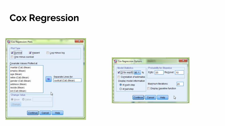
Cox Regression: Graphs

Cox Regression : Assumptions
1. The proportional hazards assumption should be fulfilled - i.e. the hazard function for the two strata should remain proportional.
2. Censoring should be non-informative i.e. censoring of one person should not influence the outcome of another
3. There is a linear relationship between the log of the hazard and the covariates
4. Overtly influential data (outliers) should not be present
There are diagnostic methods available for each of the above.

How to check for Proportional hazards1. If the predictor variable is categorical KM curves
can be generated and we can see if the lines maintain the same separate.
2. Alternatively you can generate Schoenfeld residuals in SPSS and plot these residuals against the time for each covariate.

How to check for Proportional hazards

Cox Regression : Advantages
1. It is a semi-parametric model and is less affected by outliers. 2. Unlike parametric survival models does not require correct specification of
the underlying distribution 3. Lot of diagnostic procedures
However does not give baseline hazard which makes predictive modelling
difficult

What not do while modelling (regression)
1. Do not work with sample sizes that are clearly inadequate2. Do not use univariate selection 3. Do not use stepwise forward / backward selection methods4. Do not blindly assume linearity / proportional hazards - always understand
the underlying assumptions as well as the correct checks for the same5. Read about residuals before jumping into regression6. Don’t use split sample validation - instead use cross validation or
bootstrapping
DON’T FALL IN LOVE WITH YOUR MODEL

Resources
SAS Seminar: Introduction to Survival Analysis in SAS [Internet]. [cited 2016 Sep 9]. Available from: http://www.ats.ucla.edu/stat/sas/seminars/sas_survival/
SPSS Library: Understanding contrasts [Internet]. [cited 2016 Sep 9]. Available from: http://www.ats.ucla.edu/stat/spss/library/contrast.htm
Bian H. Survival Analysis Using SPSS. Available from: http://core.ecu.edu/ofe/StatisticsResearch/Survival%20Analysis%20Using%20SPSS.pdf
Bland JM, Altman DG. The logrank test. BMJ. 2004 May 1;328(7447):1073.
Practical recommendations for statistical analysis and data presentation in Biochemia Medica journal | Biochemia Medica [Internet]. [cited 2016 Sep 8]. Available from: http://www.biochemia-medica.com/2012/22/15
Manikandan S. Measures of dispersion. J Pharmacol Pharmacother. 2011 Oct;2(4):315–6.
Manikandan S. Measures of central tendency: Median and mode. J Pharmacol Pharmacother. 2011 Jul;2(3):214–5.
Utley M, Gallivan S, Young A, Cox N, Davies P, Dixey J, et al. Potential bias in Kaplan–Meier survival analysis applied to rheumatology drug studies. Rheumatology. 2000 Jan 1;39(1):1–2.
