reference manual for moses - ultramarine.com
TRANSCRIPT
REFERENCE MANUAL FOR
MOSES
Phone (713) 975–8146 Fax (713) 975–8179
Copyright Ultramarine, Inc. June, 1989 and October 7, 2013
Contents
I. INTRODUCTION . . . . . . . . . . . . . . . . . . . . . . . . . 1II. ANALYSIS OVERVIEW . . . . . . . . . . . . . . . . . . . . . 5III. OVERVIEW OF MOSES . . . . . . . . . . . . . . . . . . . . . 8IV. MOSES BASICS . . . . . . . . . . . . . . . . . . . . . . . . . 10
IV.A The MOSES Interface . . . . . . . . . . . . . . . . . . . 11IV.B Commands, Menus, and Numbers . . . . . . . . . . . . 15IV.C Files and the ROOT Concept . . . . . . . . . . . . . . 18IV.D Customizing Your Environment . . . . . . . . . . . . . 20
V. MOSES DIMENSIONS . . . . . . . . . . . . . . . . . . . . . . 22VI. DEVICES AND PROGRAM BEHAVIOR . . . . . . . . . . . 24
VI.A Colors . . . . . . . . . . . . . . . . . . . . . . . . . . . 25VI.B Defining Styles . . . . . . . . . . . . . . . . . . . . . . . 28VI.C Logical Devices and Channels . . . . . . . . . . . . . . 30VI.D Controlling Execution . . . . . . . . . . . . . . . . . . . 34VI.E Message Commands . . . . . . . . . . . . . . . . . . . . 37
VII. GENERAL PURPOSE INTERNAL MENUS . . . . . . . . . . 39VII.A The &SELECT Menu – The Selection Process . . . . . 40VII.B The &UGX Menu . . . . . . . . . . . . . . . . . . . . . 43VII.C The &D GENERATE Menu – Document Formatting . 47VII.D The &BUILDG Menu . . . . . . . . . . . . . . . . . . . 51VII.E The &TABLE Menu . . . . . . . . . . . . . . . . . . . 53
VIII. PICTURES . . . . . . . . . . . . . . . . . . . . . . . . . . . . 55VIII.A Types of Pictures . . . . . . . . . . . . . . . . . . . . . 57VIII.B Picture Views . . . . . . . . . . . . . . . . . . . . . . . 59VIII.C Picture Selection . . . . . . . . . . . . . . . . . . . . . 62VIII.D Picture Special Effects . . . . . . . . . . . . . . . . . . 64VIII.E Picture Animation . . . . . . . . . . . . . . . . . . . . 66VIII.F Picture Ray Tracing . . . . . . . . . . . . . . . . . . . . 67
IX. ADVANCED LANGUAGE FEATURES . . . . . . . . . . . . 68IX.A Variables . . . . . . . . . . . . . . . . . . . . . . . . . . 69IX.B Loops and IF’s . . . . . . . . . . . . . . . . . . . . . . 71IX.C Macros . . . . . . . . . . . . . . . . . . . . . . . . . . . 73IX.D String Functions . . . . . . . . . . . . . . . . . . . . . . 76
IX.D.1 The &INFO String Function . . . . . . . . . . 78IX.D.2 The &NUMBER String Function . . . . . . . 80IX.D.3 The &STRING String Function . . . . . . . . 83IX.D.4 The &TOKEN String Function . . . . . . . . 85IX.D.5 The &GET String Function . . . . . . . . . . 86
IX.E Getting User Input . . . . . . . . . . . . . . . . . . . . 88IX.F Programming the Tool Bar . . . . . . . . . . . . . . . . 92
Page i

IX.G Using Files . . . . . . . . . . . . . . . . . . . . . . . . . 94IX.H Functions . . . . . . . . . . . . . . . . . . . . . . . . . 97
X. THE DISPOSITION MENU . . . . . . . . . . . . . . . . . . . 101X.A Reporting, Viewing and Storing Data . . . . . . . . . . 102X.B Adding Columns . . . . . . . . . . . . . . . . . . . . . 105X.C Recasting Data . . . . . . . . . . . . . . . . . . . . . . 108X.D Extremes and Statistics . . . . . . . . . . . . . . . . . . 110X.E Plotting . . . . . . . . . . . . . . . . . . . . . . . . . . 115X.F Getting Data . . . . . . . . . . . . . . . . . . . . . . . 118
XI. REPORT CONTROL & INFORMATION . . . . . . . . . . . 120XI.A Obtaining the Names of Quantities . . . . . . . . . . . 122XI.B Obtaining the Status of the System . . . . . . . . . . . 125XI.C Obtaining Summaries of the Model . . . . . . . . . . . 130
XII. THE MOSES MODEL . . . . . . . . . . . . . . . . . . . . . . 135XII.A Converting Models . . . . . . . . . . . . . . . . . . . . 141XII.B Defaults . . . . . . . . . . . . . . . . . . . . . . . . . . 144XII.C Parameters . . . . . . . . . . . . . . . . . . . . . . . . . 149XII.D Convolutions . . . . . . . . . . . . . . . . . . . . . . . . 153XII.E Curves . . . . . . . . . . . . . . . . . . . . . . . . . . . 154XII.F Sensors . . . . . . . . . . . . . . . . . . . . . . . . . . . 156XII.G The Environment . . . . . . . . . . . . . . . . . . . . . 158
XII.G.1 Durations . . . . . . . . . . . . . . . . . . . . 169XII.H Fatigue and Cycle Counting . . . . . . . . . . . . . . . 171
XII.H.1 Defining SN Curves . . . . . . . . . . . . . . . 173XII.H.2 Associating SN Curves with Points . . . . . . 176XII.H.3 Associating SCFs with Tubular Joints . . . . 178XII.H.4 Associating SCFs with Element Points . . . . 180XII.H.5 Beam Fatigue Due to Slamming . . . . . . . . 183
XII.I Forces . . . . . . . . . . . . . . . . . . . . . . . . . . . 185XII.J Categories and Load Types . . . . . . . . . . . . . . . . 187XII.K Bodies and Parts . . . . . . . . . . . . . . . . . . . . . 191XII.L Geometry . . . . . . . . . . . . . . . . . . . . . . . . . 203
XII.L.1 Defining Points . . . . . . . . . . . . . . . . . 205XII.L.2 Geometry String Functions . . . . . . . . . . . 208
XII.M Element Classes . . . . . . . . . . . . . . . . . . . . . . 211XII.M.1 Structural Classes . . . . . . . . . . . . . . . . 214XII.M.2 Class Shapes . . . . . . . . . . . . . . . . . . 222XII.M.3 Pile Classes . . . . . . . . . . . . . . . . . . . 224XII.M.4 Flexible Connector Classes . . . . . . . . . . . 226XII.M.5 Rigid Connector & Restraint Classes . . . . . 236XII.M.6 Propulsion Connector Classes . . . . . . . . . 238XII.M.7 Tug Connector Classes . . . . . . . . . . . . . 239
Page ii

XII.N Structural Elements . . . . . . . . . . . . . . . . . . . . 240XII.N.1 Element System . . . . . . . . . . . . . . . . . 243XII.N.2 Element Options . . . . . . . . . . . . . . . . 245XII.N.3 Beams . . . . . . . . . . . . . . . . . . . . . . 247XII.N.4 Generalized Plates . . . . . . . . . . . . . . . 253XII.N.5 Connecting Parts . . . . . . . . . . . . . . . . 260XII.N.6 Structural Post–Processing Elements . . . . . 264
XII.O Load Groups . . . . . . . . . . . . . . . . . . . . . . . . 265XII.P Compartments . . . . . . . . . . . . . . . . . . . . . . . 276
XII.P.1 Pieces . . . . . . . . . . . . . . . . . . . . . . 278XII.P.2 Defining Surfaces with Polygons . . . . . . . . 288XII.P.3 Interior Compartments . . . . . . . . . . . . . 294XII.P.4 Filling Interior Compartments . . . . . . . . . 298
XII.Q Editing a Model . . . . . . . . . . . . . . . . . . . . . . 304XIII. CONNECTIONS AND RESTRAINTS . . . . . . . . . . . . . 308
XIII.A Defining a Pulley Assembly . . . . . . . . . . . . . . . . 311XIII.B Defining a Launchway Assembly . . . . . . . . . . . . . 312XIII.C Defining a Sling Assembly . . . . . . . . . . . . . . . . 315XIII.D Defining a Pipe or Riser Assembly . . . . . . . . . . . . 317XIII.E Defining a Control Assembly . . . . . . . . . . . . . . . 319XIII.F Defining a Winch Assembly . . . . . . . . . . . . . . . 320XIII.G Altering Connectors . . . . . . . . . . . . . . . . . . . . 321
XIV. PROCESSES . . . . . . . . . . . . . . . . . . . . . . . . . . . 326XV. AUTOMATIC OFFSHORE INSTALLATION . . . . . . . . . 328XVI. THE CONNECTOR DESIGN MENU . . . . . . . . . . . . . . 345
XVI.A Obtaining Connector Tables . . . . . . . . . . . . . . . 346XVI.B Obtaining Connector Geometry . . . . . . . . . . . . . 347XVI.C Finding the Restoring Force . . . . . . . . . . . . . . . 348XVI.D Obtaining the Results for a Pile . . . . . . . . . . . . . 349XVI.E Designing a Lifting Sling . . . . . . . . . . . . . . . . . 350XVI.F Obtaining Propulsion/Weather Envelopes . . . . . . . . 351
XVII. THE REPOSITION MENU . . . . . . . . . . . . . . . . . . . 352XVIII. THE HYDROSTATIC MENU . . . . . . . . . . . . . . . . . . 354
XVIII.A Tank Capacities . . . . . . . . . . . . . . . . . . . . . . 355XVIII.B Curves of Form . . . . . . . . . . . . . . . . . . . . . . 356XVIII.C Finding Floating Equilibrium . . . . . . . . . . . . . . 357XVIII.D Longitudinal Strength . . . . . . . . . . . . . . . . . . . 358XVIII.E Righting and Heeling Arm Curves . . . . . . . . . . . . 359XVIII.F Stability Check & Allowable KG . . . . . . . . . . . . . 362
XIX. THE HYDRODYNAMIC MENU . . . . . . . . . . . . . . . . 370XIX.A Pressure Data . . . . . . . . . . . . . . . . . . . . . . . 373XIX.B Mean Drift Data . . . . . . . . . . . . . . . . . . . . . 379
Page iii
XX. THE FREQUENCY RESPONSE MENU . . . . . . . . . . . . 381XX.A Equation Post–Processing . . . . . . . . . . . . . . . . 387XX.B Motion Post–Processing . . . . . . . . . . . . . . . . . 389XX.C Cargo Force Post–Processing . . . . . . . . . . . . . . . 393XX.D Connector Force Post–Processing . . . . . . . . . . . . 396XX.E Pressure Post–Processing . . . . . . . . . . . . . . . . . 400
XXI. FINDING EQUILIBRIUM . . . . . . . . . . . . . . . . . . . . 402XXII. TIME DOMAIN SIMULATION . . . . . . . . . . . . . . . . . 405XXIII. LAUNCH SIMULATION . . . . . . . . . . . . . . . . . . . . . 408XXIV. CREATING A STATIC PROCESS . . . . . . . . . . . . . . . 410XXV. POST–PROCESSING OF A PROCESS . . . . . . . . . . . . 417
XXV.A Post–Processing Body Information . . . . . . . . . . . . 418XXV.B Post–Processing Drafts, Points, and Sensor Readings . 420XXV.C Post–Processing Compartment Ballast . . . . . . . . . 423XXV.D Post–Processing Applied Forces . . . . . . . . . . . . . 424XXV.E Post–Processing Connector Forces . . . . . . . . . . . . 426XXV.F Post–Processing Rods and Pipes . . . . . . . . . . . . . 429XXV.G Post–Processing Static Processes . . . . . . . . . . . . . 431
XXVI. STRUCTURAL ANALYSIS & APPLIED LOADS . . . . . . . 432XXVI.A Extracting Modes Of Vibration . . . . . . . . . . . . . 434XXVI.B Frequency Domain Transportation Solution . . . . . . . 435XXVI.C Defining Load Cases . . . . . . . . . . . . . . . . . . . 436XXVI.D Obtaining Applied Loads . . . . . . . . . . . . . . . . . 441
XXVII. STRUCTURAL ANALYSIS & APPLIED LOADS . . . . . . . 444XXVIII. STRUCTURAL POST–PROCESSING . . . . . . . . . . . . . 446
XXVIII.A Post–Processing Cases . . . . . . . . . . . . . . . . . . 449XXVIII.B Post–Processing & Pictures . . . . . . . . . . . . . . . . 452XXVIII.C Post–Processing Modes . . . . . . . . . . . . . . . . . . 454XXVIII.D Post–Processing Connectors & Restraints . . . . . . . . 455XXVIII.E Bending Moments and Shears . . . . . . . . . . . . . . 457XXVIII.F Force Response Operators . . . . . . . . . . . . . . . . 459XXVIII.G Post–Processing Beams . . . . . . . . . . . . . . . . . . 460XXVIII.H Post–Processing Generalized Plates . . . . . . . . . . . 464XXVIII.I Post–Processing Joints . . . . . . . . . . . . . . . . . . 466
Page iv

MOSES REFERENCE MANUAL
I. INTRODUCTION
Our primary objective with MOSES is to provide engineers with the tools necessaryto realistically design and analyze marine structures and operations. The increasingsophistication of the offshore industry, coupled with the rapid evolution of the com-putational power available, has made it obvious that to achieve this goal, a majordeparture from the traditional approaches would be necessary.
In the past, a problem was analyzed in several distinct parts – each requiring a differ-ent view of reality and subsequent model. While this approach is suited to existingorganizational structure, it is highly inefficient and error prone. Different models areipso facto different. A substantial quality assurance effort has been required to rec-oncile these differences, and more importantly, one could not hope to obtain a properanalysis of the complete picture by simply viewing selected parts of it. Obviously,what was really necessary was something that integrated all aspects of the problem.
To bridge this gap, we have created MOSES, a new language for modeling, simulating,and analyzing the stresses which arise in marine situations. This new language offersthe necessary flexibility along with the rigor of a programming language. Now, onecan easily create new models, document them, and assess their validity – all with asingle program.
In addition to specialized capabilities, the MOSES language is rich in general utilitiesto make one’s life easier. Most results of a MOSES simulation are available for inter-active reporting, graphing, viewing in three dimensions, and statistical interpretation.Instead of manually repeating blocks of data, MOSES provides for loops. Instead ofhaving different sets of data for slightly different situations, MOSES provides forconditional execution. Instead of having the same data defined in different places,MOSES allows one to define variables and use them later. Instead of repeating com-mands with minor alterations, MOSES allows the user to create his own commandscalled macros.
The MOSES language is built upon a proprietary database manager specifically de-signed for its purpose – the storage and retrieval of scientific models and the resultsof their simulations. By storing all data in a database, MOSES is totally restartable.One can perform some tasks interactively, stop, then seamlessly restart the programto perform other tasks in the background. The database even allows different typesof simulation with the same model and a stress analysis to be performed for all typesconcurrently.
Before MOSES, most marine problems were considered in two steps: a simulationfollowed by a stress analysis. Two different programs were required. Since MOSESperforms both of these analyses, one needs only a single program to investigate all
Rev Page 1

MOSES REFERENCE MANUAL
aspects of the problem. Also, with MOSES, one is spared the agony of transferringfiles and of learning the idiosyncrasies of several programs.
Since it must cope with the demands of both simulation and stress analysis, theMOSES modeling language is richer than the norm. From a stress analysis point ofview, a MOSES model consists of a set of beams, generalized plates, and connectors.Here, however, these structural elements can also model load generating attributes.To allow for other types of loads, one can define areas and masses, along with con-structs called ”hulls”. This gives MOSES the ability to compute hydrodynamic forceson a system via three hydrodynamic theories: Morison’s Equation, Two DimensionalDiffraction theory, or Three Dimensional Diffraction theory.
With MOSES, connectors are not simply ”restraints”, but the way one connectsdifferent bodies. One can select from catenary mooring lines, tension–only andcompression–only nonlinear springs, rigid connectors such as pins and launchways,and even true nonlinear rod elements. These connectors are automatically appliedduring a stress analysis so that one can correctly perform a stress analysis of severalconnected bodies.
The MOSES modeling language is rich enough so that models suitable for otherprograms can be converted to MOSES models with minimal effort. In fact, interfacesare available for several programs, and others can be quickly developed.
Not being content with simply analyzing a given situation, MOSES provides a menuwhich aids in the design of mooring lines and lifting slings. Commands are alsoavailable which will automatically alter connectors so that different scenarios can beassessed with minimal effort. With a rod connector, the effect of the inertia anddamping of the connections may be assessed.
As with connectors, MOSES allows for the basic computations traditionally per-formed by a naval architect. One can compute the curves of form, the intact ordamaged stability, and the longitudinal strength of a vessel. MOSES, however, doesnot stop here. One can specify interactively, the ballast in any or all of the vessel’stanks and immediately find the resulting condition. If one wishes, he can ask MOSESto compute a ballast plan which will achieve a given condition and then alter it. Fi-nally, if desired, one can ask MOSES to perform a detailed stress analysis of thecondition. The program will take care of all of the details of computing the correctinertia, loads, and restraints.
Once a suitable condition has been found, a traditional seakeeping study can beperformed with MOSES by issuing a single command. MOSES will then use thehydrodynamic theory selected from the three available to compute the response op-erators of both the motions of each body and the connector forces. An entire menu
Rev Page 2
MOSES REFERENCE MANUAL
of commands is available to post–process these response operators. One can easilyfind the statistical results for specified sea conditions and create time domain sam-ples of the results to assess phasing. All results can be graphed or reported. Onlyfour additional commands are necessary to produce a detailed stress analysis of thesystem in the frequency domain.
At any point, one may perform a time domain simulation of the current system. Thisis accomplished by issuing a command to define the environment, and a second toinitiate the time domain simulation. MOSES then takes the hydrodynamic forcescomputed via the proper hydrodynamic theory, combines them with the other forceswhich act on the system, and integrates the nonlinear equations of motion in the timedomain. At the conclusion, again a menu of post–processing commands are availableto assist the analyst in deciphering the results – trajectories of points, forces onelements, connector forces, etc. As before, a stress analysis at events during thesimulation requires only a few additional commands.
To simulate the process of lifting a structure off of a barge, lowering it into the water,and bringing it upright, MOSES offers a menu of alternatives. One can interactivelyballast compartments and move the hook up or down to assess the results of anyfield action. These results are stored by event so that they can be reviewed and theaction changed, until the desired outcome is attained. As with other simulations, atthe conclusion, the results can be post–processed and used for a stress analysis.
A specialized type of time domain simulation is a jacket launch. Here, a single bodyis moved until it comes free of other bodies upon which it was towed to location.Traditionally, a jacket was launched from a single barge. In anticipation of such anoperation, MOSES can simulate a launch from several barges which may be con-nected.
By combining a nonlinear rod element with other connectors, one can simulate thelaying of pipe either from a stinger or from davits. With MOSES, all aspects of theproblem can be modeled. The lay vessel and the stinger can be modeled as separatebodies connected via the pipe, hinges, tensioners, and rollers. Once the system isassembled, one can perform static, time, or frequency domain simulations of thelaying process.
MOSES can perform a detailed stress analysis for events during a time domain simu-lation, a static process, or a frequency domain process. There are no essential limitson either the model size, the number of bodies which can be analyzed, or the num-ber of load cases. The solution algorithms are state of the art and the structuralpost–processing is superior. MOSES can consider not only linear but also spectralcombinations of the basic load cases. Thus, if one performs a stress analysis in thefrequency domain, he can then consider member and joint checks spectrally. In ad-
Rev Page 3

MOSES REFERENCE MANUAL
dition, spectral fatigue can be considered in beams, generalized plates, and tubularjoints.
Rev Page 4

MOSES REFERENCE MANUAL
II. ANALYSIS OVERVIEW
MOSES is a simulation language. Thus, the commands which are available are alldesigned to either describe a system or to perform a simulation. The primary strengthhere is that the user is free to issue the commands in any order that makes sense.In other words, once a basic system has been defined, the user can alter it in manydifferent ways to change the initial conditions for similar simulations or performdifferent types of simulations, without altering the basic definition of the system.Also, after a simulation has been performed, he can analyze the deflections, stresses,etc. at different phases of the simulation.
In general, the things with which MOSES performs simulations are called bodies.During a simulation, bodies have N degrees of freedom. The first six of these are thetraditional rigid body degrees of freedom, and any others represent deformation ofthe body. Bodies are composed of smaller pieces called parts, with each part havingall of the characteristics of a body itself. MOSES is capable of considering four typesof forces which act on bodies: those which arise from water, wind, inertia, and thosewhich are applied. Thus, to MOSES, a body is a collection of attributes which tellit how to compute loads and how to compute deflections. MOSES can deal with upto 50 bodies.
In computing the forces on a body due to its interaction with the water, the user canchoose from three hydrodynamic theories: Morison’s Equation, Three DimensionalDiffraction, or Two Dimension Diffraction, the particular method used being con-trolled by the manner in which the body is modeled. A single body can be composedof any combination of hydrodynamic elements. The structure of a body can be de-fined by any combination of beam and generalized plate elements, and the user hascontrol over whether or not a given structural element will attract load from eitherwind, water, or inertia.
A second primitive element of the MOSES system is the connector. These elements,in general, attract no loads from the environment and serve to constrain the motion ofthe bodies. There are five types of connectors: flexible connectors, rigid constraints,launchways, pipes, and slings. Here, flexible connectors can be used to model mooringlines, hawsers, etc., while rigid constraints are used for pins. The user is free todefine any combination of connections. Connections are defined separately from thedefinition of the bodies, and thus, can be altered interactively to simulate differentaspects of a particular situation.
Once a system (bodies and connections) has been defined, the user is free to performstatic, frequency domain, or time domain simulations. There are also specialized setsof commands which provide information on the hydrostatics of one of the bodies,the behavior of the mooring system, or the upending of a body. The results of each
Rev Page 5
MOSES REFERENCE MANUAL
simulation are stored in a database so that they can be recalled for post–processing,restarting, or for use in a stress analysis.
After a simulation has been performed, the user can perform a stress analysis forselected parts of the system at selected events during the simulation. Here, MOSESwill compute all of the loads on the selected part at the event in question and convertthese into nodal and member loads for use by the structural solver. If the body hasmore than six degrees of freedom, then the loads applied include the deformationinertia. The restraints which correspond to the connectors will be added to thestructural model. The resulting structural system will be solved for the deflectionsat the nodes, and the deflections and corresponding element internal loads will bestored in the database.
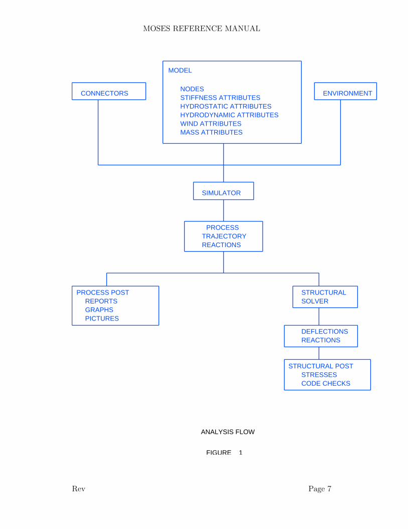
The post–processing of MOSES is one of its strongest points. Virtually all of theresults produced from either a simulation, a mooring command, or a hydrostaticcommand can be viewed at the terminal, graphed, or written to a hardcopy de-vice. In addition, many results based on the simulations can be computed in thepost–processors. In the structural analysis post–processor, code checks, joint checks,deflections, elements loads, and stochastic fatigue can be reported. These reportscan be restricted to a small subset at the request of the user. A flow chart of theprocedure just outlined is shown in Figure 1.
With the generality provided within MOSES, it is virtually impossible to delimit thetasks which can be accomplished. There are certain things, however, which can bedone simply:
• Jacket launch from one or more barges,• Time or frequency domain simulation of a structure on a system of vessels,• Time or frequency domain simulation of moored vessels,• Time or frequency domain simulation of a tension leg platform,• Docking simulation of a jacket and a pile,• Upending of a jacket,• Ballasting and stability of a vessel and cargo,• Laying of pipe from a lay vessel,• Lifting a structure from a barge,• Lowering a structure into the water,• Loadout of a structure onto a vessel,• Stress analysis of any of the above, or• Inplace analysis of a jacket.
Rev Page 6
MOSES REFERENCE MANUAL
ANALYSIS FLOW
FIGURE 1
CONNECTORS
MODEL
NODESSTIFFNESS ATTRIBUTESHYDROSTATIC ATTRIBUTESHYDRODYNAMIC ATTRIBUTESWIND ATTRIBUTESMASS ATTRIBUTES
ENVIRONMENT
SIMULATOR
PROCESSTRAJECTORYREACTIONS
PROCESS POSTREPORTSGRAPHSPICTURES
STRUCTURALSOLVER
DEFLECTIONSREACTIONS
STRUCTURAL POSTSTRESSESCODE CHECKS
Rev Page 7
MOSES REFERENCE MANUAL
III. OVERVIEW OF MOSES
Perhaps the easiest way to describe MOSES is that it is not very smart, but it has agood memory. In other words, MOSES must be told to do everything, but remembersalmost everything that it has been told. As definition, the things MOSES is told to doare called commands, while the place the results are stored is called the job database.
While all instructions to MOSES are called commands, it helps to separate instruc-tions into the categories: commands, descriptions, and questions. One issues com-mands to MOSES to accomplish tasks, issues descriptions to define a system foranalysis, and asks questions to find out the results of the commands. The databaseconsists of the union of all descriptions issued and the results of all commands. Whenone asks a question, the answers are obtained by querying the database. WhileMOSES can be utilized in both ”batch” and ”interactive” environments, it is per-haps best to view all commands as being issued from a terminal. Since the results ofall previous commands are available in the database, it is no more difficult to producea set of results by making several small runs as it is to make one big one.
The majority of the system which will be analyzed is defined to MOSES by a setof descriptions contained in the ”INPUT” file. These descriptions are commandsin what is called MOSES Modeling Language, and are processed by the programwhenever instructed by the user. When the Modeling Language is processed, thedescription is converted into an internal model within the job database so that themodel has to be processed only when it has been altered.
After a model database has been generated, the user is free to perform simulations.Before proceeding, however, one may wish to alter the definition of the system fromthat defined by the modeling language. The type of things which can be alteredare: the weight of the bodies, the connections among the bodies, or the environment.When the system is altered, the changes are again remembered until the systemis altered again. Thus, one can perform numerous simulations on the same basicsystem without rereading the model. When one issues a simulation command, thesimulation is performed, the results stored in the database, and control is returnedto the user. No reports are automatically produced, and no questions are asked, sothat simulations can easily be performed in the background. To obtain reports of theresults one must enter one of the sections of commands which were designed to answerquestions about the results of simulations. These sections of commands are calledPost–Processing Menus or Disposition Menus. In these sections of the program, onemay be asked questions himself, so it is best if these tasks are performed interactively.
The database structure of MOSES allows for ”seamless” restartability. One canterminate the program at almost any point and resume execution later with no lossof information. This structure and the root file concept discussed later free the user
Rev Page 8
MOSES REFERENCE MANUAL
from having to worry about naming, reconnecting, and remembering the names of”restart files”, and provide superior performance to previous systems. Since nothingis necessary to restart the program, nothing further will be said about it, but thecapability is one of the primary features of MOSES.
While MOSES is initially not very smart, it can learn. In other words, the user canteach the program how to perform many commands when a single one is issued. Thiscapability is implemented by allowing users to define ”macros”. These are really setsof commands which the program associates with a single name, and any time thename is issued as a command, the entire set will be executed, thus freeing the userfrom the tedious task of issuing many commands.
The flexibility of MOSES may, at first, overwhelm a new user, but with a littleexperience one quickly learns to enjoy the power of the system. In the sections whichfollow, all of the features of MOSES will be discussed. In many cases, the utilityof a feature may not be apparent when it is discussed. The primary reason is thatthere are many facets of the MOSES language which are not really necessary, butare quite useful once one has mastered the basics. Thus, instead of worrying abouthow each feature is to be used, one should proceed throughout the manual briefly toget a ”general feel” of what one can accomplish and how to do it. The next step isto carefully look over the samples supplied with this installation to see how typicalproblems may be attacked. The next step in solving a problem is to create a simpleproblem which has all of the attributes of the real, complex one to be solved and touse it as a prototype in understanding. It is always easier to use small problems tocomplete ones understanding than it is to cope with both understanding the programand with the details of a large problem.
Rev Page 9

MOSES REFERENCE MANUAL
IV. MOSES BASICS
In order to perform any task with MOSES, one must be able to communicate withthe program in a language understandable by both the user and the program. In thissection, the rules of grammar and syntax of the language employed and the generaloperation of MOSES will be discussed.
In discussing the various types of commands, some of the words are ”set off”. By ”setoff”, we mean the words are either underlined or printed in bold type, depending onthe method used to print this manual. These words are keywords, either commands oroptions, and must be input exactly as written. The characters not ”set off” representthe data which takes on the appropriate numeric or alphanumeric value. In somecases, an underline is part of an option or command. For example, END DISPOSEis a command. In keeping with the format of this manual, these commands are ”setoff” (and possibly underlined), and the user needs to remember that the underlineexists as part of the command.
MOSES provides many features of a programming language. In MOSES, one canalter the flow of either command or description input, make logical checks, definevariables, create macros, etc. All of these features operate on both commands anddescriptions, so that with this language one can automate the definition of a modelas well as build a set of specific commands he needs to perform repetitive tasks.
Rev Page 10

MOSES REFERENCE MANUAL
IV.A The MOSES Interface
MOSES actually has four different user interfaces. By default, it starts in ”GUI”mode. The other three are a terminal, a ”silent” interface, and the old GUI mode,which we refer to as the window interface.
Silent Interface
With the silent interface, MOSES produces no terminal output except that directedby the internal command &S BACK. This option is quite useful for running MOSESin a ”pipe”. While the details discussed here differ slightly between the graphical andterminal interfaces, the operation is much the same. MOSES is, and at heart willremain, a language where commands are input and results produced. The graphicalinterfaces are simply more efficient at their job.
Terminal Interface With the terminal option, MOSES simply runs in the existingterminal (or console) window. It only has a display area and commands are inputdirectly into it. With a terminal interface, the actual commands listed must be usedand none of the keyboard shortcuts are operative. Of course pictures or graphics canonly be viewed in one of the graphic interfaces. A WINDOWS command promptwill not properly display a MOSES terminal session. To use this type of interfaceon WINDOWS machine, you should start a ”MinGW sh” and use it to run MOSES.You should navigate to c:/ultra/bin/win32/msys (or wherever MOSES is installed).Here you will find a shortcut to msys. You can drag this to your desktop, doubleclick on it, and a window will open. Be warned that this window is a UNIX shell andhere you will need to use / instead of \ for path separators.
GUI Interface
This is the standard interface for interactive MOSES sessions. The interface consistsof six parts:
The Menu should be familiar to users of the previous versions of MOSES. New tothis version is the Help menu which takes you to the new hyperlinked help systemavailable in this release.
The Top Button Bar is where you’ll find features that are used often or are onlyfound in this interface (not in the ”–text” or –”win” interfaces).
• Save lets you save wire frame or GL images as you see them. The currentpicture is added to your graphics device file.• Copy will copy either text or graphics to the clipboard for use in other programs.
Rev Page 11
MOSES REFERENCE MANUAL
• Paste will paste text from the clipboard to the current cursor position.• Help brings up the new hyperlinked, indexed help system.
The Left Button Bar
These controls are specifically for the graphics windows, and are documented in theControls section.
The Right Side Bar
The right SideBar is currently used to display information about the model in 3Dgraphics mode. The user can use the select tool to get information about any partof the model. This SideBar is customizable and scriptable from MOSES macros.
The Main Workspace
The Main workspace has three parts to it: the command line, the tabs, and the datawindow, which can be either text or graphic. The command line is the standardMOSES command line and accepts standard MOSES commands. The text datawindow shows the same MOSES output the user is accustomed to. The graphical datawindows can show standard MOSES pictures, MOSES graphs, and the new OpenGLpictures. The Tab system allows the user to open and interact with multiple pictures.It should be noted, though, that entering the MEDIT menu will cause all picturesto be closed, as the model data may have changed. When a tab containing a pictureis in focus, there will be a ”control panel” at the bottom of the picture. This panelcontain (from left to right): a window showing the current process, a button settingthe speed of an animation to half the normal speed, a button for playing/stoppingthe animation, a slider showing the events, and a box where you can pick the view.When the picture is created, it will show the last event in the current process.
The Status Bar
The Status Bar currently shows whether MOSES is Busy or Ready for another com-mand, as well as showing what command will actually be executed when the mousemoves over an item in the menu.
Window Interface
The window interface presents the user with a window containing four basic areas:a tool bar, a display area, a command line box, and a scroll bar. The display areais used to give you information during a program session. This information is alsowritten to a file, the ”log file” so that you can review it later. The information isscrollable so that you can look at any portion of it any time a command is expected.
Rev Page 12
MOSES REFERENCE MANUAL
As you will see below, the display can be toggled back and forth between the log, theuser manual, and for a window interface, a picture.
The tools bar can be used to change settings and obtain reports without actuallyinputing the commands to do so. At the moment, it does not entirely suffice in placeof the command line but in the future it will. When you push one of the buttons onthe tool bar, a menu will ”drop down”. In this new menu, buttons which are ”plane”will immediately do what the title says. Those which end in a > will drop downanother level of menu. To clear a menu, you should push the top area which is blankexcept for a <. A large tree of menus can be cleared by simply hitting an ”Enter”.
Keyboard Shortcuts
There are special keys that are mapped to commands, or which move one about inthe display. They are in either display:
&FINISH – Ctl F&PICTURE – Ctl P&PICTURE –RENDER GL – Ctl G&PICTURE –RENDER WF – Ctl W@TOP – the home key@BOTTOM – the end key+P – the page up key–P – the page down key!– – the up cursor key!+ – the down cursor key
The first of these command terminates MOSES. The next three change to ”picturemode” with the first using the type of picture last rendered as the type, and the othertwo using the render mode specified (G for a GL picture, W for a wire frame). Seethe section on Pictures for details. These four shortcuts are always available. Theremainder of them discussed here work only when one is focused on the text displayor the command line.
The next four commands simply move the user’s reading position. @TOP put onea the beginning of the display and @BOTTOM at the end. +P command movesup a page and –P moves down one.
The last two commands move up and down one command in the command history.In addition to storing the entire terminal input/output history, MOSES also saves arecord of the commands which have been issued. While there are numerous uses ofthis command log, the primary one is to allow the user to see ”where he is”. This is
Rev Page 13

MOSES REFERENCE MANUAL
accomplished by the !P command, the form of which is:
!P, NUMB(1), NUMB(2)
When this command is issued, a portion of the command log will be printed to theterminal. If no option is specified, then the commands printed will be preceded bythe command number, and if –N is specified as an option, then the numbers will notbe printed. If neither NUMB(1) nor NUMB(2) is specified, then the last commandissued will be printed, and if NUMB(1) is a negative number then the commandsfrom the current number plus NUMB(1) to the current number will be printed. IfNUMB(1) is an *, then the entire log will be printed, and if both NUMB(1) andNUMB(2) are positive the commands between the two numbers will be printed. Forexample, !P 10 20 lists all the commands between command number 10 and 20. !P10 20 –N does the same thing, except no command number will be printed. !P –10will show the last 10 commands.
Another benefit of the command log is that previous commands can be re–executedby either the command:
!, PHRASE
or by the method discussed below. Here, PHRASE can be either nothing, a number,or a string. If it is nothing, the last command executed will be place in the commandbox so that it can be edited and executed. This is equivalent to the cursor up key ona window interface. Repeated use of the cursor up key will move up the commandhistory. If it is a number, MOSES will simply execute the specified command. If itis a string, then MOSES will search up the command log until it finds a commandcontaining STRING and will then execute that command.
Rev Page 14
MOSES REFERENCE MANUAL
IV.B Commands, Menus, and Numbers
Each input record can contain three types of data. The first word on the recordis called the command or description name and it conveys to the program the typeof data being communicated with this record. The format of all records does notrequire that the data be in any particular column, but instead, the various datais separated by a comma, or by as many blanks as desired. The remainder of theinformation on the record is of two types: DATA or –OPTIONS. DATA must be inthe order specified, while –OPTIONS may be in any order. So that the program candistinguish between data and options, all options begin with a –. If the last wordof a record image is a \, then the following record is a continuation of the currentrecord. Also, the option lists consist of data which may or may not be needed. Asmany pieces of this data as required can be specified in any order, and usually consistof an alphanumeric ”option keyword” followed by the corresponding alphanumericor numeric data. Alphanumeric names may consist of up to eight characters, andnumeric values may contain up to twenty characters. The general form of a commandline is:
COMMAND, DAT1, DAT2, ... –OPTION1 OD11, OD12, ....., \–OPTIONn ODn1, ODn2, ......
While the options can be input in any order, sometimes different results may beobtained with a different order of the options. This will occur when the data usedby one option is altered by another one. MOSES parses options from left to right, sooptions which change data that another option will use should be placed first.
When it comes to the actual task of defining a number to MOSES one can accomplishthe task in many ways. The flexibility is due to the fact that the command inter-preter will perform a conversion of numerical data in accordance with FORTRANconventions for arithmetic. In other words, a number can be defined as a series ofnumbers combined by primitive numerical operations.
As an example, consider the number 64. The following representations would all yieldthe same value:
61+38**2(6+2)*8((35–1)–2)*4/2
While this ability may appear to be of limited utility, it proves to be quite powerful
Rev Page 15
MOSES REFERENCE MANUAL
when combined with the more advanced language features.
To simplify the operation and documentation of the program, MOSES employs theconcept of menus. A menu, as used here, is an available list of commands which cancurrently be executed. If an attempt is made to execute a command which is notcontained in the current list, a message to that effect will be reported, and a promptfor another command will be made. There are several menus in MOSES. When anEND command is issued, MOSES will return to the next higher menu. To terminateexecution of MOSES one simply inputs an &FINISH command, which is a validcommand in any menu. In a window environment, the key Alt F can be used insteadof typing in &FINISH.
There are several commands within MOSES which can be executed regardless of thecurrent menu. These commands are called Internal Commands. In general, theycontrol the operation of the program, set basic variables which effect the analysis,and can be distinguished by the fact that they all begin with the character &. Anexample is the &FINISH command, which is valid regardless of the current menu.The primary importance of an internal command is that it can be issued from eitherthe INPUT or COMMAND channel, therefore, it can be set once in the INPUTchannel, and later reset interactively.
MOSES uses minimum uniqueness to identify a command in the current list. By this,we mean that only enough of the command need be specified so that the programcan uniquely define the intended command. If the command issued is not unique,all valid commands which match the one issued will be printed, and a prompt fora unique response will be given. If one issues a null command (a simple carriagereturn) MOSES will print a list of all the currently valid commands. For InternalCommands, minimum uniqueness in not employed. Instead, one need only specify thefirst five characters of the command name. Also, notice that MOSES uses minimumuniqueness for commands, but not for modeling language commands. In other words,commands which enter through the INPUT channel must be specified completely withthe exception of internal commands.
MOSES has the notion of an escape character. This character is used to ”remove” anyspecial meaning associated with the following character. Here, the escape characteris the \. An example of the use of this character was shown previously with thecontinuation of a command line. In this context, the character is used to escape theend of the line. If one actually wishes to input a \, he must use \\. This is particularlyimportant on a PC when this character is used in defining directory paths.
In addition to the special characters discussed above, MOSES employs several others.A full list of the special characters are:
Rev Page 16

MOSES REFERENCE MANUAL
\ used to remove the special meaning of the following character, and to providefor command line continuation.
$ used to denote the end–of–record. Any data which follows this character isignored (hence it is useful for adding comments.)
/ used to denote the wild character. One or more of these may be placed anywherein an alphanumeric name.
@ used to denote some number of wild characters. If this character is placed in aname, it acts like some number of wild characters, /.
’ used to delimit a name which contains blanks and/or commas. The name mustbe enclosed by a pair of ’s.
” used to repeat command names or for a second level of quoting. If this is thefirst word of a record, the first word of the previous record will be used. If it isencountered in a position other than the command position, it act the same asa ’. Here, it allows for a double level of including blanks.
– The first character of an option name. The option is usually followed by a listof parameters in order to specify some desired action.
& The first character of an internal command.
: The first character of a selection criteria.
* The first character of a point name.
# The first character of a load attribute.
∼ The first character of an element stiffness attribute name.
Rev Page 17
MOSES REFERENCE MANUAL
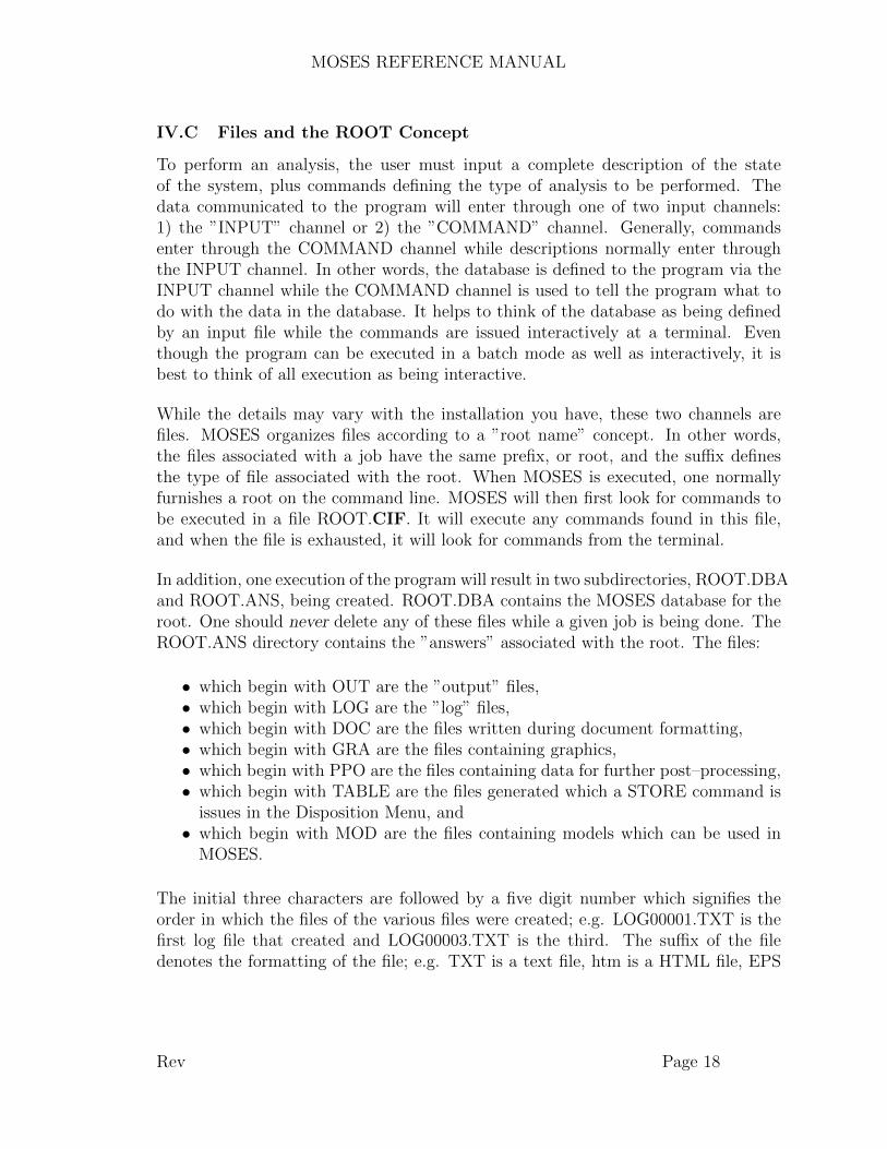
IV.C Files and the ROOT Concept
To perform an analysis, the user must input a complete description of the stateof the system, plus commands defining the type of analysis to be performed. Thedata communicated to the program will enter through one of two input channels:1) the ”INPUT” channel or 2) the ”COMMAND” channel. Generally, commandsenter through the COMMAND channel while descriptions normally enter throughthe INPUT channel. In other words, the database is defined to the program via theINPUT channel while the COMMAND channel is used to tell the program what todo with the data in the database. It helps to think of the database as being definedby an input file while the commands are issued interactively at a terminal. Eventhough the program can be executed in a batch mode as well as interactively, it isbest to think of all execution as being interactive.
While the details may vary with the installation you have, these two channels arefiles. MOSES organizes files according to a ”root name” concept. In other words,the files associated with a job have the same prefix, or root, and the suffix definesthe type of file associated with the root. When MOSES is executed, one normallyfurnishes a root on the command line. MOSES will then first look for commands tobe executed in a file ROOT.CIF. It will execute any commands found in this file,and when the file is exhausted, it will look for commands from the terminal.
In addition, one execution of the program will result in two subdirectories, ROOT.DBAand ROOT.ANS, being created. ROOT.DBA contains the MOSES database for theroot. One should never delete any of these files while a given job is being done. TheROOT.ANS directory contains the ”answers” associated with the root. The files:
• which begin with OUT are the ”output” files,• which begin with LOG are the ”log” files,• which begin with DOC are the files written during document formatting,• which begin with GRA are the files containing graphics,• which begin with PPO are the files containing data for further post–processing,• which begin with TABLE are the files generated which a STORE command is
issues in the Disposition Menu, and• which begin with MOD are the files containing models which can be used in
MOSES.
The initial three characters are followed by a five digit number which signifies theorder in which the files of the various files were created; e.g. LOG00001.TXT is thefirst log file that created and LOG00003.TXT is the third. The suffix of the filedenotes the formatting of the file; e.g. TXT is a text file, htm is a HTML file, EPS
Rev Page 18

MOSES REFERENCE MANUAL
is a postscript file, etc.
The OUT files contains all of the hardcopy reports you requested and the LOG filescontain the commands issued and and MOSES responses to the commands.
Rev Page 19

MOSES REFERENCE MANUAL
IV.D Customizing Your Environment
In the directory where the software is installed, there is a subdirectory named data.This subdirectory stores data required for the execution of the software and files thatallow the user to customize an installation. The data directory is further dividedinto subdirectories. The ones of interest here are named local, progm and site.The files moses.aux, moses.mac, moses.man and moses.pgm are stored in theprogm directory. These files contain auxiliary shapes data, program macros, the online reference manual and program parameters and default settings, respectively. Alsoat this directory level is the original moses.cus file provided with the installation.
The files in the progm directory are read each time the program is executed as partof program initialization, and should not be altered by the user. The local directoryis provided for user customization. When the program is executed, it checks for theexistence of a local database. If these do not exist, then it builds them. During thebuilding of these databases, the program will attempt to read files moses.mac andmoses.aux from the local directory. This allows one to add a set of site specificmacros and structural shapes to those which are normally available. You shouldsimply create files with the above names and then delete the file moses.sit on aUNIX machine or moses.dsi on a PC. The next time the program is executed, thedatabases will be recreated with your data included.
Most customization that one needs is available with the moses.cus file. This processis even easier than that described above. There can be many different copies ofmoses.cus, and they are read in order. First, the copy in the data/progm directoryis read, next, the one in data/local. These are basically used to set variables for theentire network. After these two, MOSES looks for two more: first in location definedwith the environment variable $HOME (%HOME% in WINDOWS), and then in thecurrent working directory. The last two of these allow for customization at the userand job level. If you are homeless (do not know your home), you can find it by typingin a command prompt:
echo %home% – on WINDOWS, orecho $home – on anything else
The ”cus” file contains MOSES commands that localize MOSES for your situation.In addition, there is another set of files which contain user preferences. MOSES looksfor moses.ini or .moses.ini in each of the location it looks for moses.cus. Whenlooking in the MOSES install directories, the name without the . is used and inthe home and local directories, the name with the . is used. The ini files are againsimple text files that you can edit with a text editor, but you can also maintain the.moses.ini file in your home directory directly in MOSES. Simply use the Customize
Rev Page 20
MOSES REFERENCE MANUAL
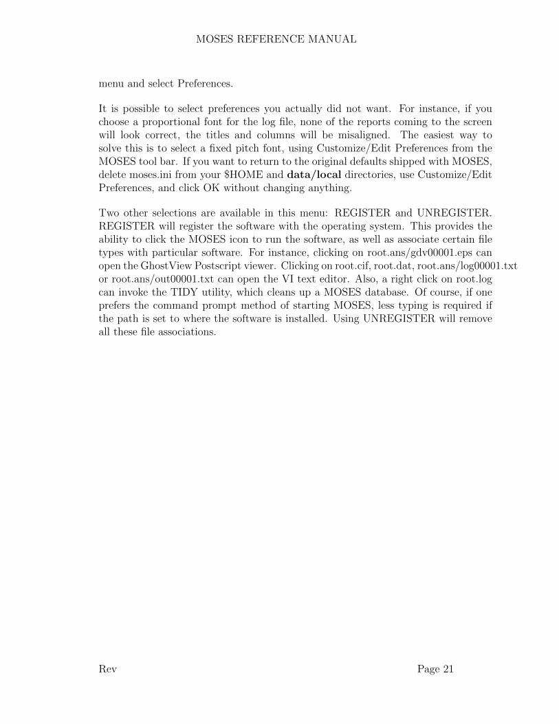
menu and select Preferences.
It is possible to select preferences you actually did not want. For instance, if youchoose a proportional font for the log file, none of the reports coming to the screenwill look correct, the titles and columns will be misaligned. The easiest way tosolve this is to select a fixed pitch font, using Customize/Edit Preferences from theMOSES tool bar. If you want to return to the original defaults shipped with MOSES,delete moses.ini from your $HOME and data/local directories, use Customize/EditPreferences, and click OK without changing anything.
Two other selections are available in this menu: REGISTER and UNREGISTER.REGISTER will register the software with the operating system. This provides theability to click the MOSES icon to run the software, as well as associate certain filetypes with particular software. For instance, clicking on root.ans/gdv00001.eps canopen the GhostView Postscript viewer. Clicking on root.cif, root.dat, root.ans/log00001.txtor root.ans/out00001.txt can open the VI text editor. Also, a right click on root.logcan invoke the TIDY utility, which cleans up a MOSES database. Of course, if oneprefers the command prompt method of starting MOSES, less typing is required ifthe path is set to where the software is installed. Using UNREGISTER will removeall these file associations.
Rev Page 21
MOSES REFERENCE MANUAL
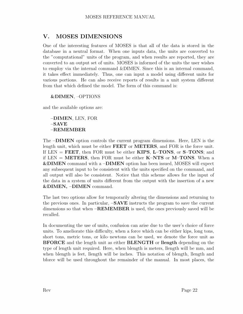
V. MOSES DIMENSIONS
One of the interesting features of MOSES is that all of the data is stored in thedatabase in a neutral format. When one inputs data, the units are converted tothe ”computational” units of the program, and when results are reported, they areconverted to an output set of units. MOSES is informed of the units the user wishesto employ via the internal command &DIMEN. Since this is an internal command,it takes effect immediately. Thus, one can input a model using different units forvarious portions. He can also receive reports of results in a unit system differentfrom that which defined the model. The form of this command is:
&DIMEN, –OPTIONS
and the available options are:
–DIMEN, LEN, FOR–SAVE–REMEMBER
The –DIMEN option controls the current program dimensions. Here, LEN is thelength unit, which must be either FEET or METERS, and FOR is the force unit.If LEN = FEET, then FOR must be either KIPS, L–TONS, or S–TONS; andif LEN = METERS, then FOR must be either K–NTS or M–TONS. When a&DIMEN command with a –DIMEN option has been issued, MOSES will expectany subsequent input to be consistent with the units specified on the command, andall output will also be consistent. Notice that this scheme allows for the input ofthe data in a system of units different from the output with the insertion of a new&DIMEN, –DIMEN command.
The last two options allow for temporarily altering the dimensions and returning tothe previous ones. In particular, –SAVE instructs the program to save the currentdimensions so that when –REMEMBER is used, the ones previously saved will berecalled.
In documenting the use of units, confusion can arise due to the user’s choice of forceunits. To ameliorate this difficulty, when a force which can be either kips, long tons,short tons, metric tons, or kilo–newtons can be used, we denote the force unit asBFORCE and the length unit as either BLENGTH or llength depending on thetype of length unit required. Here, when blength is meters, llength will be mm, andwhen blength is feet, llength will be inches. This notation of blength, llength andbforce will be used throughout the remainder of the manual. In most places, the
Rev Page 22

MOSES REFERENCE MANUAL
units required for a given quantity are specified. If they are omitted, they are:
Quantity Unitstime – secondsangles – degreestemperature – degrees F or degrees Clength – feet or metersarea – ft**2 or m**2volume – ft**3 or m**3velocity – ft/sec or m/secacceleration – ft/sec**2 or m/sec**2stress or pressure – ksi or mpaforce – bforcemoment – bforce–blengthweight per unit length – bforce/blengthweight per unit area – bforce/blength**2
Rev Page 23

MOSES REFERENCE MANUAL
VI. DEVICES AND PROGRAM BEHAVIOR
Perhaps one of the most confusing things which MOSES does is dealing with devices.By device, we mean either a physical piece of hardware such as a printer, pen plotter,terminal screen, or logical device such as a file. In MOSES there are two concepts:a channel and a logical device. Basically, channels can be thought of as either filesor as directly connected physical devices. Logical devices are different classes ofoutput which are ”connected” to a channel. As data is written to a logical device,it is formatted according to a set of instructions collectively called a style. In thefollowing pages, each of these concepts will be defined in detail. For most of thethings defining device attributes, the units required are points. A point is 1/72 of aninch or .3527 mm. The exception to the above rule is when one defines the ”pitch”of a fixed pitch font which is defined in characters per inch.
Rev Page 24

MOSES REFERENCE MANUAL
VI.A Colors
Colors in MOSES are treated by first defining a set of colors which may be used andthen assigning individual colors to a ”color scheme”. Color schemes are then used byassigning them to styles (which are discussed below), or by special names which areused to draw the user interface window.
Both colors and color schemes are defined with the command:
&COLOR NAME –OPTIONS
To define a color, NAME should be omitted and the option:
–COLOR ADD, C NAME, RVAL, GVAL, BVAL
should be used. Here, C NAME is the name of the color to be defined and RVAL,GVAL, and BVAL are the intensities of red, green, and blue respectively. Thesevalues are 0 for none of this color and 255 for the maximum of this color. Thus, todefine yellow, one should use
&COLOR –COLOR ADD YELLOW 255 255 0
By default, there are over 400 colors already defined (more than the colors in theX11 file rgb.txt). To see what colors are predefined, one can use the command:
&COLOR –NAMES
The &COLOR command is also used to define the color maps used for pictures; i.e.the map which maps ratios and intensities to colors. This is accomplished with theoptions:
–S MAP, C NAME(1), C NAME(2), .... C NAME(n)
and
–R MAP, C NAME(1), C NAME(2), .... C NAME(n)
Here, –S MAP defines the color map used for stress coloring and –R MAP definesthe map for ratio coloring. C NAME(i) are the names of colors and there can be fromtwo to 128 names. If d = 1. / (N – 1) where N is the number of names specified,then C NAME1 is used for ratios between 0 and d, C NAME(2) between d and 2d,... C NAME(n–1) between (n–2)d and 1, and C NAME(n) for ratios greater than 1.
The final thing accomplished with the &COLOR command is the definition of color
Rev Page 25

MOSES REFERENCE MANUAL
schemes. A color scheme is two sets of colors, one ”normal” the other ”special”.Each of these has: a background color, a foreground color, box edge colors, selectedcolors, and line colors. The normal colors are those used except when a special effectis desired: Reverse video for something selected in a menu, or a line that is belowthe water. The option:
–USE, C NAME
causes MOSES to load up the color scheme C NAME and then what follows will onlychange what is in C NAME. Thus, if one uses this option he need only specify thosethings that he wishes to be different from C NAME. Likewise, if one issues:
&COLOR NAME .....
and the color scheme NAME exists, then he is actually editing NAME. There areseveral color schemes predefined in MOSES: DEFAULT, BASIC FRAME, BASIC,MENU, WIDG FRAME, WIDGET, and H COPY. The first of these is the basis formost things. BASIC, BASIC FRAME and MENU are used for the components ofthe MOSES User Interface Window and WIDG FRAME and WIDGET are used forthings that ”pop up” in this window. H COPY is used for things which are writtento hardcopy devices. In general, the only difference between these is the color of thebackground.
All of these colors themselves are defined with the options:
–N BACKGROUND, C NAME–S BACKGROUND, C NAME–N FORGROUND, C NAME–S FORGROUND, C NAME–N BEDGE, C NAME(1), C NAME(2)–S BEDGE, C NAME(1), C NAME(2)–N SELECT, C NAME(1), C NAME(2)–S SELECT, C NAME(1), C NAME(2)–N LINES, C NAME(1), C NAME(2), .......... C NAME(6)–S LINES, C NAME(1), C NAME(2), .......... C NAME(6)
The options –N BACKGROUND and –S BACKGROUND define the back-ground colors. Here (and what follows), the prefix –N defines ”normal” colors and –S defines ”special” ones. The options –N FORGROUND and –S FORGROUNDdefine the foreground colors. The options –N BEDGE and –S BEDGE each definetwo colors. The first color is for a sunken box and the last for a raised box. The op-tions –N SELECT and –S SELECT also define two colors, the first for quantitiesselected and the second for those not selected. Finally, the options –N LINES and
Rev Page 26

MOSES REFERENCE MANUAL
–S LINES define six colors for ”logical lines 1 – 6”. These are used in both graphsand pictures. For example when drawing a graph, the foreground color is used forthe border and the axes and line color 1 is used for the first curve, line color 2 forthe second curve, etc.
Rev Page 27
MOSES REFERENCE MANUAL
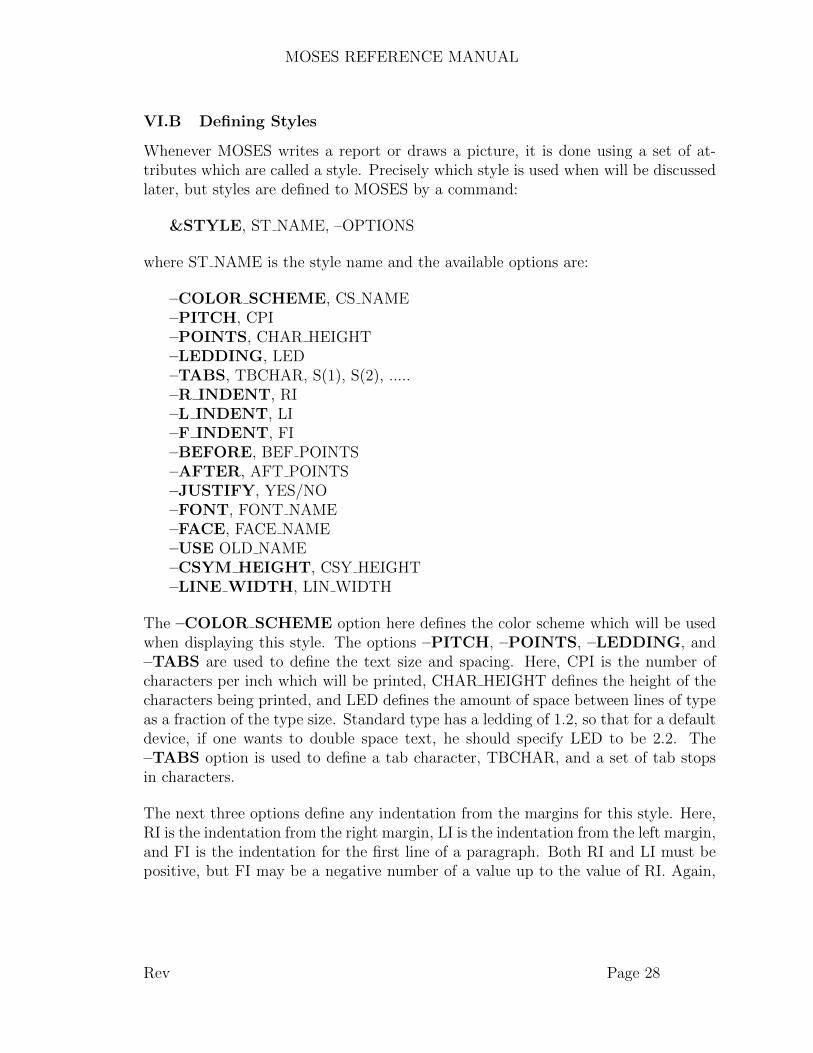
VI.B Defining Styles
Whenever MOSES writes a report or draws a picture, it is done using a set of at-tributes which are called a style. Precisely which style is used when will be discussedlater, but styles are defined to MOSES by a command:
&STYLE, ST NAME, –OPTIONS
where ST NAME is the style name and the available options are:
–COLOR SCHEME, CS NAME–PITCH, CPI–POINTS, CHAR HEIGHT–LEDDING, LED–TABS, TBCHAR, S(1), S(2), .....–R INDENT, RI–L INDENT, LI–F INDENT, FI–BEFORE, BEF POINTS–AFTER, AFT POINTS–JUSTIFY, YES/NO–FONT, FONT NAME–FACE, FACE NAME–USE OLD NAME–CSYM HEIGHT, CSY HEIGHT–LINE WIDTH, LIN WIDTH
The –COLOR SCHEME option here defines the color scheme which will be usedwhen displaying this style. The options –PITCH, –POINTS, –LEDDING, and–TABS are used to define the text size and spacing. Here, CPI is the number ofcharacters per inch which will be printed, CHAR HEIGHT defines the height of thecharacters being printed, and LED defines the amount of space between lines of typeas a fraction of the type size. Standard type has a ledding of 1.2, so that for a defaultdevice, if one wants to double space text, he should specify LED to be 2.2. The–TABS option is used to define a tab character, TBCHAR, and a set of tab stopsin characters.
The next three options define any indentation from the margins for this style. Here,RI is the indentation from the right margin, LI is the indentation from the left margin,and FI is the indentation for the first line of a paragraph. Both RI and LI must bepositive, but FI may be a negative number of a value up to the value of RI. Again,
Rev Page 28
MOSES REFERENCE MANUAL
RI, LI, and FI are measured in points.
The –BEFORE and –AFTER options define the number of points of blank spacewhich will be set before or after a paragraph, while the –JUSTIFY option is usedto define whether or not the right margin of the text will be justified. If YES/NO isNO, the margin will not be justified.
The –FONT option is used to define the type style which will be used, and thevalue for FONT NAME must be either LGOTHIC or COURIER. The –FACEoption defines the character of the type, and FACE NAME must be either: NOR-MAL, UNDERLINE, BOLD, ITALICS, or BITALICS. Here, NORMAL willbe standard type, UNDERLINE will be underlined, etc.
The –USE option is used to create a new style based on a previously defined one,OLD NAME. If used, this should be the first option specified, and it instructs MOSESto use the previous style as the default values for the current style.
The last two options are used when pictures or graphs are being produced. The–CSYM HEIGHT option defines the height of any centered symbols on a graph.These are normally used to differentiate between two curves, or to denote points.The –LINE WIDTH option defines the width of any lines being drawn.
Rev Page 29

MOSES REFERENCE MANUAL
VI.C Logical Devices and Channels
In MOSES the concepts of channel and logical device are quite similar. A logical de-vice is simply an additional layer of abstraction which allows one to achieve preciselythe results he wishes. We will begin with the process of defining a logical devicewhich is accomplished by the command:
&LOGDEVICE, LDVNAM, –OPTIONS
and the available options are:
–CHANNEL, CHANAM–STYLE, T STYLE, N STYLE, A STYLE–MARGIN, IM, OM, TM, BM–LANDSCAPE, YES/NO–PSOURCE, TRAY
Here, LDVNAM is the logical device name which must be either: LOG, OUTPUT,SCREEN, GRA DEVI, DOCUMENT, TABLE, PPOUT, or MODEL. Theselogical devices serve to provide output for screen reports, hard copy reports, screengraphics, hard copy graphics, hard copy documents, stored tables, post–processinginformation, and MOSES model data respectively. The options serve to define the ap-pearance of the results. The –CHANNEL option associates a channel with the logi-cal device. More will be said about channels later, but the valid values for CHANAMare exactly the same as for LDVNAM.
The –STYLE option defines a style which will normally be used when writingthings to this logical device. For graphics devices, three styles can be specified withT STYLE defining the style for text on the graphics, N STYLE the numbers, andA STYLE the axes.
The –MARGIN option defines the margins for a page in points. IM and OM definethe ”inside” and ”outside” margins, and TM and BM define the top and bottommargin. The –LANDSCAPE option can alter the orientation of the print on thepaper. If YES/NO is NO, the results are placed on the paper so that they shouldbe read with the ”long edge of the paper” on the left. If YES/NO is YES, then thepage will be rotated 90 degrees. The margins are a property of the paper itself withthe program taking care of the details when landscape and double sided printing areperformed. The –PSOURCE option selects the current paper tray. Here, TRAYmust be either UPPER or LOWER, and this option only works for certain physical
Rev Page 30

MOSES REFERENCE MANUAL
devices.
Channels are defined with the command:
&CHANNEL, CHANAM, –OPTIONS
where the available options are:
–PAGE DIMEN, WIDTH, HEIGHT–DOUSIDE, YES/NO–P DEVICE, PDVNAM, LEVEL–FILE, FILE–SINGLE, YES/NO
Basically, this command associates a true physical device with the channel, CHANAM,and the valid values for CHANAM are those given for LDVNAM. Here the –PAGE DIMENoption defines the size of a page on the channel in points,and the –DOUSIDE optioninstructs the printer to print on both sides of the paper, and currently works only onPCL devices.
The physical devices which can be connected to channels are defined with the –P DEVICE option. Here valid values of PDVNAM are: SCREEN, DEFAULT,POSTSCRIPT, TEX, PCL, JPG, PNG, UGX, DXF, HTML, or CSV. If thephysical device is PCL, then LEVEL defines the PCL level for the device, whichmust be either 3, 4, or 5. Here, the physical device SCREEN does double duty inthat it is specified for both the LOG and graphics screen channels, and the particularbehavior of the SCREEN depends upon the user interface one is using.
Normally, logical devices of the same name are associated with these channels, butit is not necessary. More will be said about this later. Not all physical devices canbe connected to all channels. In particular:
• LOG can only be connected to DEFAULT or SCREEN physical devices.• OUTPUT can only be connected to DEFAULT, TEX, POSTSCRIPT, or PCL
physical devices.• SCREEN can only be connected to DEFAULT or SCREEN physical devices.• GRA DEVI can only be connected to UGX, POSTSCRIPT, DXF, JPG, or
PNG physical devices.• DOCUMENT can only be connected to DEFAULT, TEX, POSTSCRIPT, or
PCL physical devices.• TABLE can only be connected to HTML or CSV physical devices.• PPOUT can only be connected to DEFAULT physical devices.
Rev Page 31
MOSES REFERENCE MANUAL
• MODEL can only be connected to DEFAULT physical devices.
With the exception of the SCREEN, channels are connected to files. For example,the results for channel OUTPUT will be written to the file OUTXXXXX.TXT inthe ROOT.ANS directory. In general, the file name is the first three characters ofthe channel names followed by a five character number and having a suffix whichcorresponds to the physical device. Here, the physical device/suffixes are:
DEFAULT txtPOSTSCRIPT epsTEX texPCL pclDXF dxfJPG jpgPNG pngUGX ugxHTML htmCSV csv
If you want to change the directory where the ”answer files” are stored, you can usethe command &FILE USE discussed below. If you want to change the location ofthe file for a given channel, you can use the –FILE can be used. Normally all of thegraphics for a given run will be stored in a single file (except for types of JPG orPNG). This can be changed with the –SINGLE option where a YES/NO of YESwill result in each frame of graphics being written to a separate file.
Each time a &CHANNEL is issued, the file currently connected to the channel willbe closed and a new file will be used. For example, suppose GRA00001.eps is the filecurrently connected to the GRA DEV channel. Then the command
&CHANNEL GRA DEV
will result in GRA00001.eps being closed and the next graphics will be written toGRA00002.eps. If GRA00001.eps is empty, then nothing will happen.
It may seem odd that the available channels and logical devices are the same, butit offers quite a bit of flexibility. For example if one has a postscript printer, thenhe only needs one of the channels OUTPUT, DOCUMENT, or GRA DEV, and hecan connect all three of these logical devices to it. This makes the results of all threelogical devices appear in order when printed. A drawback of this approach, however,is that once the OUTPUT logical device is formatted for a particular device it may
Rev Page 32
MOSES REFERENCE MANUAL
become unreadable.
The TEX device is actually a file written in a format that can be processes by thepopular text formatting program LaTeX. When this device is connected to the DOC-UMENT channel, it generates a stand alone file for input into LaTeX. Included inthis file is a set of macros which ”make it work”. When connected to the OUTPUTchannel, the file is not complete in that it is missing the macros, the prologue, the”begin document” and the ”end document” statements. This occurs since one nor-mally wants to input the output file into the document file to produce a completedocument.
The DXF and UGX physical devices are for saving graphical results. The DXFdevice is used to store MOSES graphics into DXF format. The UGX device wasdesigned as a page description language, and is more completely defined later. Whenthis device is used, the file can be read by MOSES and converted to a graph on thespecified logical device. In particular, graphics saved in this format can be viewed onthe screen by simply issuing the command:
&INSERT GRA00001.UGX
Also, if the primary graphics device is the GRA DEV logical device, then the abovecommand will format the graphics for a hard copy device.
For any channel which has a physical device of PCL, the results in the file containescape sequences which control the device. Thus, files representing these channelsshould be sent to the device in raw form. If MOSES is being run on a PC, these filesshould be copied to the printer using the /B option on the DOS COPY command.This avoids the DOS spooler treating the printer escape sequences as end of line orend of file characters.
Rev Page 33
MOSES REFERENCE MANUAL
VI.D Controlling Execution
The user also has the ability to control the various parameters which effect the exe-cution of MOSES and the various files which will be used. Perhaps the most usefulof these commands is:
&DEVICE, –OPTIONS
and the available options are
–BATCH, YES/NO–LIMERROR, ERLIM–US DATE, YES/NO–SET DATE, DATE–CONT ENTRY, The Entry You Want–NAME FIGURE, NAME–FIG NUM, YES/NO, NUMBER–G DEFAULT, GLDEVICE–OECHO, YES/NO–MECHO, YES/NO–IDISPLAY, YES/NO–SILENT, YES/NO–FN LOWER, YES/NO–COMIN, FILE NAME–ICOMIN, FILE NAME–AUXIN, FILE NAME–IAUXIN, FILE NAME
These options can be roughly divided into several classes. The –BATCH optiondefines when the program will terminate abnormally. Here, YES/NO should beYES if one wishes to set the mode to batch, and NO if one wishes the executionmode to be interactive. The –LIMERROR option defines the error limit. If theprogram is in the ”interactive” mode, it will terminate when the error limit, ERLIM,is reached. This limit is defined by the –LIMERROR option. In the ”batch” mode,MOSES will terminate when any error is encountered.
The next set of options define the way dates and figures are printed. The –US DATEcontrols the style of the date which will be printed on the output reports. If YES/NOis YES, the date will be the month, followed by the day, followed by the year. IfYES/NO is NO, then the day will be printed first, followed by the month, followedby the year. The –SET DATE options allows one to actually set the date stringto the string which follows. The –CONT ENTRY option allows one to definethe next entry which will be added to the table of contents. If the string follow-
Rev Page 34
MOSES REFERENCE MANUAL
ing the option key word is blank, then MOSES will revert to the default behavior.The –NAME FIGURE option allows one to define the string which will be puton graphics along with a figure number. The default here is ”FIGURE”. The –FIG NUM option instructs MOSES whether or not to put figure numbers on plots,and perhaps what number to use. If YES/NO is YES, then ”Figure XX” will beplaced in the lower left corner of all plots not directed to the screen. Here, XX is anumber which will be 1 for the first plot, 2 for the second, etc. If YES/NO is NO,no figure numbers will be plotted. If ”NUMBER” is specified, then the next figureplotted will have the number specified.
The next option is used to alter the destination of graphic output. There are twoplaces where graphics can be deposited: the primary place and the secondary one.When a PICTURE or PLOT command is issued, the results are automatically writtento the primary place and when a SAVE is issued, the results are written to thesecondary place. The –G DEFAULT option defines the default logical device forgraphics. Here GLDEVICE must be either SCREEN, or FILE, which will defineeither the SCREEN, or GRA DEVICE logical device to be the device wheredefault graphics is written.
The next class of options controls the type of output which is received. The –OECHO option is used to control the listing of output. If the YES/NO followingthis option is YES, then each record from the input file is written to the output fileas the record is read. Conversely, if YES/NO is NO, the echo will not occur. The–MECHO option will instruct MOSES to echo commands which are being executedas part of a macro to be echoed to either the terminal (and therefore the log file), orto the output file. Macros being used in the input data will be echoed in the outputfile if the –OECHO YES/NO is YES. The options –IDISPLAY, and –SILENTcontrol the default displays. The option –IDISPLAY controls whether or not thevalid internal commands will be displayed whenever valid commands are listed. The–SILENT option suppresses most of the terminal output, and is useful in macros.For all of these options, the action will be taken if YES/NO is YES, and not ifYES/NO is NO.
The –FN LOWER option controls the way MOSES looks at the directory structure.If YES/NO is NO then the directory structure is viewed as case sensitive. In someoperating systems it really does not matter even if then results appear in upper andlower case. In other words a file COW.TXT is a different file from cow.txt. One maynot want this behavior (transferring files from a WINDOWS machine to a UNIX onefor example). In this case one can use the option with a YES/NO of YES. Now thecomplete path of the file will be treated as being lower case.
The final class of options controls where the program obtains its information. Ingeneral, commands enter through the ”command channel”, TERM, and data en-
Rev Page 35

MOSES REFERENCE MANUAL
ters through the ”input channel”, INPUT. With the –COMIN option MOSES getscommand data from the file, FILE NAME, until either an end of file is encountered,MOSES finishes, or another –COMIN command is specified. The –AUXIN optionfunctions as the –COMIN option except that it redirects the flow of information onthe INPUT channel. With both of these options, if FILE NAME is &E then MOSESreturns to the default channel. With these two options, a fatal error occurs if the filespecified does not exist. If one does not desire an error if the file does not exist, thenhe can use either –ICOMIN or –IAUXIN. With these two options, the commandis simply ignored if the files fail to exist. In some cases, one does not know whetherhe wishes to redirect the input or the command channels, but instead he wishes toredirect the ”current” channel. This can be accomplished by using the command:
&INSERT, FILE NAME
Here, the current information channel will obtain its data from the file FILE NAMEas discussed above.
Rev Page 36
MOSES REFERENCE MANUAL
VI.E Message Commands
MOSES allows the user to issue messages to both the ”output” and ”command”channels via internal commands. For the output channel, the messages are limitedto two title lines of data which are printed at the top of each page of output. Thesecan be defined via:
&TITLE, MAIN TITLE&SUBTITLE, SUBTITLE
Here, MAIN TITLE is used for the first title line, and SUBTITLE is used for thesecond title line.
To issue messages to the command channel, one uses the commands:
&TYPE, MESSAGE&CTYPE, MESSAGE&CUTYPE, MESSAGE
These commands will write ”MESSAGE” to the terminal whenever they are executed.The difference between the commands is that the &TYPE command left justifiesthe output line, while the other two center the line on the screen. The &CUTYPEcommand not only centers the line, but also underlines it.
If one is writing macros, it is often necessary to report to the user an error or warning.This is accomplished with the command:
&ERROR, CLASS ,MESSAGE
Here, CLASS is the class of warning and can be either WARNING, ERROR, orFATAL, and MESSAGE is the message you wish to have printed along with the class.If CLASS is FATAL then the program will terminate after printing the message.
In addition, there is a menu which can be used to define reports:
&REPORT, HEAD(1), HEAD(2) –OPTIONS
and the available options are
–HARD–BOTH
The report generated will have a primary heading of HEAD(1) and a secondaryheading of HEAD(2). If no options are specified, it will be written to the terminal. If
Rev Page 37

MOSES REFERENCE MANUAL
–HARD is specified, it will be written to the output file, and if –BOTH then it willbe written to both devices. The menu is exited with an END REPORT command.
Inside this menu, the commands
TYPE, MESSAGECTYPE, MESSAGECUTYPE, MESSAGE
are available. These commands are exactly the same as those discussed above.
Rev Page 38

MOSES REFERENCE MANUAL
VII. GENERAL PURPOSE INTERNAL MENUS
MOSES has several features of a general nature which are quite useful. These willbe discussed in this section before the more specific abilities are considered.
Rev Page 39
MOSES REFERENCE MANUAL
VII.A The &SELECT Menu – The Selection Process
When communicating with MOSES, one must often select data from a set. For ex-ample, when one issues a command, he is really selecting one command for processingfrom a set of valid commands. In contrast, there are cases where one may select morethan one item from the set. In either case, data must be given to MOSES so that aselection can be made. In most cases, the data will consist of the names of the itemsto be selected. Since simply issuing the names can become cumbersome, MOSESuses a more general method, the Selector.
A Selector can be a name, a name containing either @’s or /’s, or a Selection Criteria.Here, a / is a ”wild character” which stands for any character, and an @ stands foran arbitrary number of characters. In many cases, the word MATCH will be used.By a match, we mean that two names are equivalent to within the wild characters.As an example, each of the following strings match the other:
ABCDEFGHA/CDEFGHA@H
A Selection Criteria is a more general method of selecting data. In essence, it is aname ( :SEL NAME, which must begin with a : ) with which two sets of selectorsare associated. The first set of selectors ( S NAME(i) ) define a set of names whichwill be selected. The second set ( E NAME(i) ) define a set of names which will beexcluded.
The objective of the selection process is to take a set of values and to apply a selectionrule which will result in a ”selected” subset. The selector :SEL NAME operates onthe admissible set in two steps. The first is to search the entire list of values for amatch with any of the S NAMEs. This results in a subset which is then subject toexclusion by the second step. In other words, the results of the first step are checkedfor a match against any of the E NAMEs. If a match is found, that item is removedfrom the selected set.
A special menu is provided to define and examine selection criteria. This menu isentered via the command:
&SELECT
and the valid commands are:
END &SELNAME, :SEL NAME, –OPTION
Rev Page 40
MOSES REFERENCE MANUAL
SELECT, S NAME(1), S NAME(2), ....., S NAME(n)EXCEPT, E NAME(1), E NAME(2), ....., E NAME(n)INFO SEL, :SEL NAME, –OPTIONLIST SEL, –OPTION
The first of these commands define the ”current” selection criteria name. All of thecommands which follow will deal with the ”current” name until it is redefined. If nooption is included, then the action which follows will be added to the existing defini-tion of the selection criteria. To ”start over” one should use the option –DELETEon the NAME command. This will remove any previous data defined for the selec-tion criteria. The two commands SELECT and EXCEPT are used to define thenames for selection and exception respectively. The LIST SEL command gives a listof selection criteria which have been defined, and the INFO SEL command givesthe specific S NAMEs and E NAMEs for the selection criteria :SEL NAME. BothLIST SEL and INFO SEL accept the option –HARD. If this option is omitted,the reports will be written to the terminal, if it is included, they will be written tothe output file.
If no S NAMEs are defined for a given :SEL NAME, then all of the available list willbe selected in the first step, and if no E NAMEs are defined, then all values selectedby the S NAMEs will be selected. Thus, a :SEL NAME which has not been definedwill select everything.
As an example of how to assemble these commands, consider:
&SELECTNAME :COWSELECT 1, 2, 3, 4, M@EXCEPT M1, M2, M3NAME :DOGSELECT D@
END &SEL
Here, two selection criteria are defined, :COW and :DOG. The first one selects 1, 2,3, 4 and everything beginning with M except M1, M2, and M3. :DOG simply selectseverything beginning with a D.
In many cases, one can define a selection criteria quickly by using the abbreviatedcommand:
Rev Page 41

MOSES REFERENCE MANUAL
&SELECT, :SEL NAME, –OPTIONS
where the options are:
–SELECT, S NAME(1), ....., S NAME(n)–EXCEPT, E NAME(1), ....., E NAME(n)
With the abbreviated form of the command, the selectors defined in the exampleabove can be quickly defined by:
&SELECT :COW –SELE 1, 2, 3, 4, M@ \–EXCEPT M1, M2, M3
&SELECT :DOG –SELE D@
Rev Page 42
MOSES REFERENCE MANUAL
VII.B The &UGX Menu
As was mentioned previously, MOSES has a language for describing a picture on apage. There are two uses of this format: A way to ”save” graphics for later viewing,and a way to define pictures. The &UGX Menu allows pictures to be converted fromthe UGX format into some other format. Alternately, one can use the commands inthis menu to generate pictures of his own creation.
The UGX Menu is different from most menus in that it is accessible only though amacro! Each trip into the &UGX Menu is used to produce a single page of graphics.To enter this menu, one simply issues:
&UGX, WHAT, WHERE
where WHAT is the name of a previously defined macro and WHERE can be usedto alter the definition of the logical device to which the picture will be written.WHERE must be either: SCREEN, DEVICE, or SAVE, and if it is omitted, thenthe picture will be written to the primary graphics device.
A valid UGX macro is like any other macro except that it contains the commandslisted below and it has the command
END &UGX
as its last command. For example,
&MACRO LINEMOVETO 0 0LINE 20 20END &UGX&ENDMACRO&UGX LINE
will cause a picture to appear on the screen consisting of a single line.
Several commands are available to create pictures. The origin of the coordinatesystem is in the upper left hand corner of the page, the x axis is parallel to the top ofthe page, and the y axis is parallel to the left hand side of the page. All dimensionsgiven here are in points. To allow for a UGX picture to be correctly mapped ontoany device, the command:
BBOX, X MAX, Y MAX
will automatically establish a non–distorting scale so that the picture will fit on the
Rev Page 43

MOSES REFERENCE MANUAL
current physical page. Here, X MAX and Y MAX are the maximum X and Y valueswhich are used in the picture. Notice that by the choice of origin, there are nonegative X or Y coordinates in this system.
To allow one flexibility in defining a picture, one can change the frame of referenceat will by issuing the command:
TRANSFORM, XO, YO, –OPTIONS
and the available options are:
–SCALE, X SCALE, Y SCALE–ANGLE, ANGLE–MATRIX, Q11, Q21, Q12, Q22
After this command is issued, a transformation from the input coordinates to theframe described above is established which works as follows:
o = t + Q*S*i
Where the two components of t are defined by XO and YO, the Q matrix is definedby either ANGLE or the components of Q, and the S matrix is a diagonal matrixwith components given by X SCALE and Y SCALE. Normally, one does not needthe –MATRIX option and instead defines the transformation via the –ANGLEoption. Here, ANGLE is the angle in degrees through which the original x axis mustbe rotated to yield the new x axis. This rotation is positive toward the original yaxis.
As with all output operations in MOSES, the &UGX commands are performedaccording to a style. To establish the current style here, one issues the command:
STYLE, C STYLE
Where C STYLE is the style which will be used for all subsequent drawing. One canalso change the color by issuing the command:
COLOR, COLOR NUM
where COLOR NUM is a line color number. The association of line color numbersand colors was discussed previously.
Pictures are created by combining lines and text, and for each primitive, drawingbegins at the ”current cursor position”. The current cursor position can be defined
Rev Page 44

MOSES REFERENCE MANUAL
by the command:
MOVETO, X, Y
To draw a generalized line, one issues:
LINE, X(2), Y(2), ......, X(n), Y(n)
This command will draw n–1 straight line segments beginning at the current cursorlocation and ending at the coordinates X(n), Y(n). At the conclusion of the drawing,the current location will be at X(n) and Y(n). To fill a polygon in the current color,one uses:
FILL, X(2), Y(2), ......, X(n), Y(n)
which works the same way as LINE does.
Three other primitives are available for drawing lines. To draw a rectangle, one canissue:
BOX, X DIM, Y DIM
The resulting rectangle will have the upper left corner at the current location and itwill have a width of X DIM and a height of Y DIM. At the conclusion, the currentlocation will remain unchanged. To draw a circular arc, one issues:
ARC, RADIUS, ANG(1), ANG(2)
The center of the arc is at the current location and the arc will have a radius ofRADIUS. The arc will be drawn from the angles ANG(1) to the angle ANG(2).These angles are measured from the x axis positive toward y. If the two angles areomitted, a circle will be drawn. The current location is not changed by this command.The final line primitive draws a line with an arrow at the end of it, and is defined by:
DLINE, X2, Y2
The line is drawn from the current location to the point X2, Y2 and the arrow isplaced at the second end. At the conclusion, the current location is at X2, Y2.
Four commands are available to annotate the picture. The command:
CSYMBOL, CSYM NUM
will produce a ”centered symbol” of a type defined by CSYM NUM at the current
Rev Page 45
MOSES REFERENCE MANUAL
location. CSYM NUM is an integer from 1 to 9, where each number produces adifferent type of symbol. To write text, one has three commands available, none ofwhich moves the current location. The command:
TEXT, ANGLE, TXTSTR
will write the string of text defined by TXTSTR beginning at the current location.The text will be at an angle, ANGLE, from the x axis. If ANGLE is omitted, zerowill be used. The current location is not effected by this command. Another way ofdrawing text is with the command:
CTEXT, X2, Y2, TXTSTR
Here, the text string defined by TXTSTR is centered between the two points definedby the current location and X2, Y2. The text is drawn with the beginning of thestring toward the current location so that the bottom of the text is parallel to theline between the two points. A similar command is:
DIMENSION, X2, Y2, TXTSTR
This command draws text the same way as CTEXT, but it also draws dimensionlines between the two points.
Finally, if one is merging a page in UGX into other graphics generated by MOSESwith figure numbers, the UGX figure should also be numbered. This is accomplishedby issuing the command:
FIG NUM, X, Y
which will place the figure number at the coordinates specified by X and Y.
Rev Page 46
MOSES REFERENCE MANUAL
VII.C The &D GENERATE Menu – Document Formatting
To allow one to fully utilize MOSES’s database structure, a text formatting capabilityis provided. This formatter basically takes input text and formats it according toa set of given instructions for a specified output device. To simplify matters, thisprocess occurs within an internal menu, entered via the command:
&D GENERATE, –OPTIONS
The available options are:
–CMD, CMD FILL CHAR–SAVE–NO CONT
The –CMD option is used to alter the ”internal command character” which will beused in this menu. Normally, this character is the &. The other two options controlwhat is done with the results when the document formatter is exited. The –SAVEoption instructs MOSES to save the current settings for page numbers, etc., and the–NO CONT option says not to write a table of contents. To exit this menu, oneissues a command:
CMD FILL CHAREND
Here CMD FILL CHAR is the same character specified with the –CMD option; i.e.if no –CMD option were issued, the menu would be exited with
&END &D GENERATE.
The basic job of the document formatter is to take a paragraph of text and rearrange itaccording to a user defined ”style” which was discussed earlier and a set of formattingcommands. Formatting commands are enclosed within a pair of { and }. To associatea given style with a paragraph, one should use the formatting command
{STYLE, ST NAME}
The style ST NAME will be used for all paragraphs until another style name isselected. Notice that if one uses a style before it is defined, an error will result. Noticethat this is the general form of a formatting command; a { immediately followed bya command name, followed by a token delimiter, followed by data for the command,and finished with a }.
Until now, paragraphs have been discussed, but not defined. MOSES uses a methodof implicit paragraph generation. In other words, a paragraph is a collection of lines
Rev Page 47

MOSES REFERENCE MANUAL
delimited by either a line beginning with a blank, or certain formatting commands.This scheme works well for most text, but on occasion, one wishes to format thetext himself. To allow for this, MOSES can operate in the ”pre–formatted” mode,where text is simply transmitted to the output device without rearranging it. In thepre–formatted mode, each line is a paragraph. To enter this mode, one issues theformatting command:
{PRE}
and to exit:
{!PRE}
In addition to the general commands described above, there are several others avail-able which may expedite special tasks. In particular
{SKIP, POI REL}{MOVE, POI ABS}{EJECT}{EODD}
allow for positioning text on a page. Here, POI REL is a number of points relativeto the current position at which the next text will be printed, and POI ABS is aabsolute position on a page where the next text will be printed. The {EJECT} and{EODD} commands cause next text to be printed on a new page. The !EODDcommand will create a blank page if the current page is an odd numbered one, andthe document is double sided.
To control the general appearance of the pages, one can use
{RPAGNUM, NUMB}{HEAD, TEXT}{FOOT, TEXT}
The first of these commands sets the ”current” page number to be NUMB, and{HEAD} and {FOOT} are used to define headers and footers. The styles usedfor headers and footers are HEAD and FOOT respectively. The TEXT on a headeror footer can be any one line of text containing positioning instructions, and it cancontain the special symbol #, which will be replaced with the current page numberwhen the text is written. For both footers and headers, the –BEFORE option of thestyle defines how far down from the bottom margin or top of the page the header or
Rev Page 48

MOSES REFERENCE MANUAL
footer will be printed.
In many instances, one is producing a document which requires a table of contentsand which has sections. This is facilitated by the commands:
{SECTION, TEXT}{PART, TEXT}{SUBPART, TEXT}{BPAGE, TEXT}{CONTENTS, TEXT}{INDEX, TEXT}
For the first three of these commands, a section label will be created, the sectionheading will be printed using the style SECTION, and a table of contents entry willbe generated. The next command will simply create a blank page with a single lineof text in the center of it. The next command will either place the table of contentsat this position in the document or create a place for it. The last command will placethe index at this position in the document.
In addition to the general formatting via styles, MOSES has the ability to temporarilyoverride styles within a paragraph. This is accomplished by enclosing parts of thetext within a set of delimiters. To set some text bold, one should use
{b}
at the beginning of the bolding and
{dc}
at the conclusion. Likewise for underlining one uses
{U}
at the beginning and
{!U}
at the end. For italics, one uses the pairs {I} and {!I}.
Often on wishes to format a ”list” of things. This is accomplished by entering the”LIST” mode with:
Rev Page 49
MOSES REFERENCE MANUAL
{LIST, LIST TYPE –OPTIONS}
Here LIST TYPE is the type of list and must be chosen from ITEMIZE or USE FIRST;and if omitted, ITEMIZE will be used. A LIST TYPE of ITEMIZE will put a ”bul-let” as the beginning of each list item while USE FIRST will use the first non–blankcharacter in the list as the item delimiter. Now, the list is composed of ”items” whichare simply paragraphs. To exit LIST mode, one uses:
{!LIST}
There is one option:
–SPACE, SPACE
which defines the vertical space in points at the beginning and end of the list.
The final formatting construct is ”TABLE” mode which is entered with
{TABLE, TABLE TITLE, –OPTIONS}
and exited with
{!TABLE}
A table consists of a centered title, TABLE TITLE, and a matrix. The matrix isdefined as each paragraph being a row. The general definition of a table row is
|column(1)|column(2) ..... |
where the beginning of the row is indented (rows are viewed as paragraphs). The |delimit the definition of the elements within the row. By default, the element will becentered within the column width. If one does not wish the elements to be centered,he can use < or > as the first character of a part to either left or right justify thepart within the column. There is one option:
–MARK, SEP CHAR
which is used to change the column separation character from | to SEP CHAR. Adegenerate list of a single row can be simply defined with
{CENTER |part(1)|part(2) ..... |}
This table will have no title.
Rev Page 50
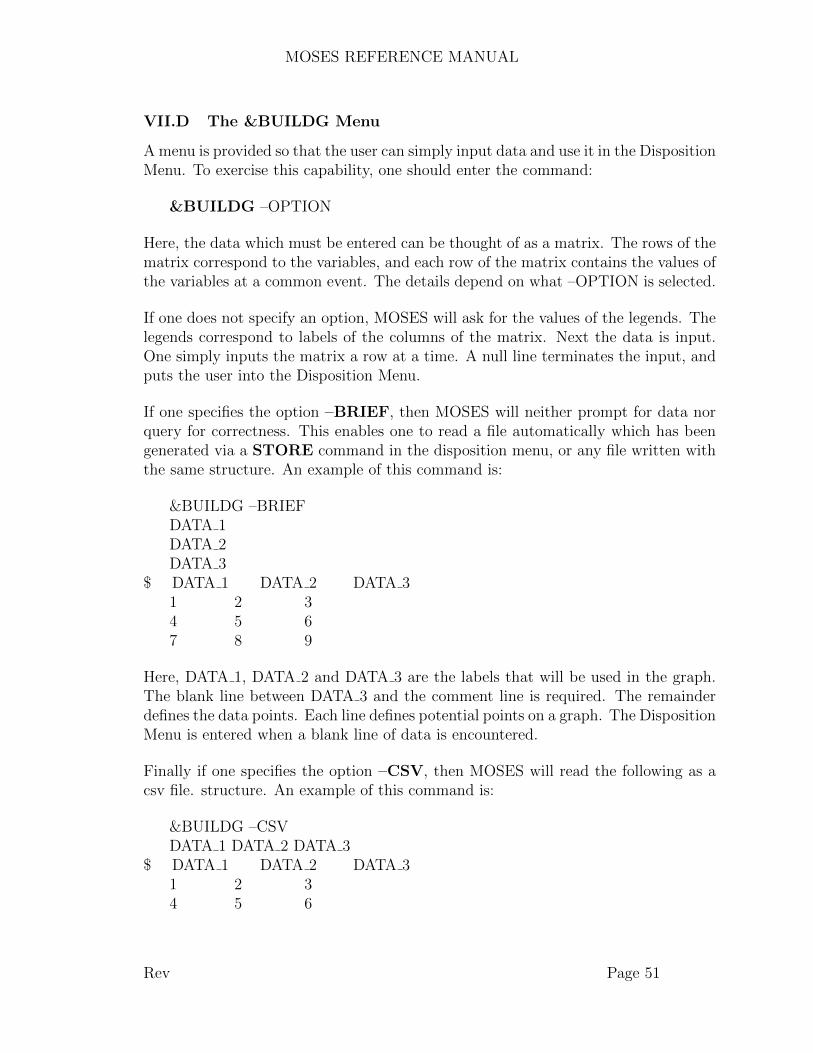
MOSES REFERENCE MANUAL
VII.D The &BUILDG Menu
A menu is provided so that the user can simply input data and use it in the DispositionMenu. To exercise this capability, one should enter the command:
&BUILDG –OPTION
Here, the data which must be entered can be thought of as a matrix. The rows of thematrix correspond to the variables, and each row of the matrix contains the values ofthe variables at a common event. The details depend on what –OPTION is selected.
If one does not specify an option, MOSES will ask for the values of the legends. Thelegends correspond to labels of the columns of the matrix. Next the data is input.One simply inputs the matrix a row at a time. A null line terminates the input, andputs the user into the Disposition Menu.
If one specifies the option –BRIEF, then MOSES will neither prompt for data norquery for correctness. This enables one to read a file automatically which has beengenerated via a STORE command in the disposition menu, or any file written withthe same structure. An example of this command is:
&BUILDG –BRIEFDATA 1DATA 2DATA 3
$ DATA 1 DATA 2 DATA 31 2 34 5 67 8 9
Here, DATA 1, DATA 2 and DATA 3 are the labels that will be used in the graph.The blank line between DATA 3 and the comment line is required. The remainderdefines the data points. Each line defines potential points on a graph. The DispositionMenu is entered when a blank line of data is encountered.
Finally if one specifies the option –CSV, then MOSES will read the following as acsv file. structure. An example of this command is:
&BUILDG –CSVDATA 1 DATA 2 DATA 3
$ DATA 1 DATA 2 DATA 31 2 34 5 6
Rev Page 51

MOSES REFERENCE MANUAL
7 8 9END
Rev Page 52

MOSES REFERENCE MANUAL
VII.E The &TABLE Menu
A menu is provided so that the user can simply input data and have it written aseither a CSV (comma separated value) or a HTML file. To exercise this capability,one should enter the command:
&TABLE –OPTION
followed by as many records as necessary to define the rows of the table. You shouldhave the same number of tokens in each row (input record) and if you want to havespaces in a token, you should delimit the token with either a ” or a ’. To have a cellblank, you can use either ” ” or NA or NOT USED. The following options controlthe appearance of the table:
–HEADING, HEAD–TITLE, NCOL(1), CT(1), .... NCOL(n), CT(n)–BOLD, YES NO–H SKIP, YES NO–ROW SHADE, YES NO–FIGURES, COL SEL, RIGHT–EXTR SHADE, COL SEL(1), COL SEL(2), .....–V LINES, COL SEL(1), COL SEL(2), .....
After defining the rows, you should end the table with
END &TABLE
The –HEADING and –TITLE options define the text at the top of the table andyou probably want more than one of each. The headings and titles are emitted inthe order the options are specified and the headings are emitted before the title. Ifthe –BOLD option is specified with YES NO if YES then the titles and headingswill be set in ”bold” type, and if the –H SKIP option is specified with YES NO ofYES then a line will be skipped between each heading. In actuality, headings aresimply a title which spans all of the columns of the table. Titles, however, can spanNCOL(i) columns.
The –ROW SHADE option instructs MOSES to shade the rows two at a time. Ifthis option is selected with YES NO of YES you will get two white rows followedby two rows shaded in light green. The –FIGURES option offers a way to changethe display of the numbers. It says to change the number of figures after the deci-mal point for columns selected by COL SEL to be RIGHT figures. You can specifymore that one –FIGURES option. The –EXTR SHADE option is used to definethe columns for which the maximum and minimum values will be shaded in a dif-
Rev Page 53

MOSES REFERENCE MANUAL
ferent color. Here, COL SEL(i) are selectors for the columns which will be shaded.COL SEL(i) can be a single number which selects that mode number, or a pair ofnumbers A:B which selects all modes from A to B. The –V LINES option definesthe columns where vertical lines will be drawn at the right. Vertical lines are alwaysdrawn at the left of column 1 and to the right of the last column. If you have acolumn selector of 1, then a vertical line will be drawn between columns 1 and 2.
For CSV tables, the –H SKIP, –BOLD, –ROW SHADE, –EXTR SHADE,and –V LINES options have no effect.
Rev Page 54
MOSES REFERENCE MANUAL
VIII. PICTURES
As mentioned above, one can obtain a picture of the current situation by issuing thecommand the &PICTURE command. This command is used to get pictures ofeverything, and as a result, it has options to control:
• The type of data used in the picture,• The title of the picture,• The portion of global space to paint,• The ”annotation” of the picture,• The production of a deflected shape picture,• The use of color in the picture, and• The names of things included in the picture.
Once something is specified on a &PICTURE command, it is remembered throughout a MOSES session, unless however, it is changed. There are Tool Bar controls forall of the things on the picture command as well as a set of keyboard shortcuts tomake life easier.
There is quite a bit of data which can be defined to create a picture which is preciselywhat one wants. To make it easier to reproduce these pictures, MOSES employs theconcept of a ”user defined view”. One defines a view with the command:
&PI VIEW –OPTION, V NAME, ......
Here, V NAME is the name which will be given to the view, and the data whichfollows is any data which can be placed on the &PICTURE command. The –OPTION may be either –ADD or –DELETE. For –DELETE, only V NAME isrequired. Now, once a view has been defined, a picture can be produced with
&PICTURE, V NAME, ....
Here, V NAME is the name of a view defined via &PI VIEW, and what followscan be nothing or any valid &PICTURE data. If additional data is specified, itmodifies the picture defined in V NAME. To make it easy to plot all of ”your” views,you can use the string function:
&NAMES(PI VIEW)
which returns all of the user defined views.
The form of the command is:
Rev Page 55

MOSES REFERENCE MANUAL
&PICTURE, VIEW DATA –OPTIONS
With so much going on here, it is easy to get a picture which is worthless. The option:
–RESET
will reset the defaults so that something appears.
By default, the current title and subtitle are placed at the top of the picture. Theoptions –TITLE and –SUBTITLE can be used to alter these values.
–TITLE, M TITLE–SUBTITLE, S TITLE
The
–RENDER R TYPE
option defines the manner in which the picture will be rendered. If you are in the GUIuser interface, you can specify a R TYPE of SOLID to have the picture renderedas a picture of solid objects. Alternative, a R TYPE of WF will render the picturesas a ”wire frame”. WF rendering is the only thing available with a WIN interface.When rendering a solid picture, connectors are rendered as lines so that they willappear regardless of their diameter and/or distance. If, however, you exercise theoption
–CON SOLID YES/NO
with a value of YES, then they will be rendered as round elements with the properdiameter.
Finally, a picture that has been created may be written to a file for later processingby using the option
–SAVE PIC
The file used by this command is specified on the –SECONDARY option of the&DEVICE command.
Rev Page 56
MOSES REFERENCE MANUAL
VIII.A Types of Pictures
The type of data used to construct a picture is specified with the option
–TYPE, TYPE
Here, TYPE must be selected from DEFAULT, STRUCTURE, MESH, or COM-PARTMENT. When this option is used, the selected data appropriate to the TYPEspecified will be extracted from the database, converted into ”strings” which can beplotted, and stored in a different portion of the database. If an &PICTURE com-mand is issued within the &SURFACE MENU, then blocks will be used instead ofthe current TYPE. The TYPE DEFAULT will show all exterior compartments andany beams which have load attributes.
There are two levels of control over the data to be plotted. First, one can selectparts of the model by using the options for a &REP SEL command issued prior toselecting a TYPE. Only data selected will then be passed to the picture painter. Ad-ditional control is available in the picture painter itself. Each string is assigned namesfor: NAME, BODY, PART, ENDS. PARENT, and PIECE. The ”NAME” of astring is the element names if it is a structural element or connector, the panel nameif it is a panel, or the load group name if it is a load group attribute. The ”BODY”and ”PART” are the obvious choices except for connectors where their BODY andPART is GROUND. The ”ENDS” of a string are simply the points at the ends ofthe string.
”PARENT” and ”PIECE” are a bit more abstract and the definition depends on thetype of string. For structural elements with load attributes the ”PIECE” is SLATand for those without load attributes, it is SELE. The ”PARENT” for all structuralelements is the element class. For connectors, the piece is CONNECTOR and theparent is the element class. For panels, the piece is the piece name and the parentis the compartment name. For load group attributes the piece is either: #BUOY,#TUBE, #AREA, #PLATE, #WEIGHT, or #LSET depending upon how itwas defined, and the parent is the load group name. If one is viewing pictures fromthe &SURFACE MENU, then block names replace compartment and piece names inthe above scheme.
To obtain pictures of the panels which will be used in a three dimensional diffractionanalysis, one should use the TYPE MESH. With this TYPE, one can use the option–DETAIL and MOSES will generate a refined mesh for plotting which correspondsto current settings of the –M DIST option of the &PARAMETER command.
In addition to these ”names”, the strings have numbers associated with them. Ingeneral, these numbers are a ratio, a cdr, a stress, and a deflection. Only nodes will
Rev Page 57

MOSES REFERENCE MANUAL
have a deflection associated with them. These numbers can be used in the picturepainter to alter the color mapping so that one can pictorially represent somethingother than the configuration. Only joints, beams, and plates have a cdr or cumulativedamage ratio. Connectors have a ratio which corresponds to their current unityratio. Compartments have a ratio which is their current percent full. The numbersassociated with the structural elements are assigned in the Structural Post–ProcessingMenu. Until one enters this menu, all numbers will be zero. For nodes, the ratiois the maximum punching shear unity ratio for all load cases, the deflection is thelast deflection reported with a JOINT DISPLACEMENT command, and the stressis zero. For beams, the ratio is the maximum code check ratio for all load cases, thestress is the largest Von Mises stress divided by is yield that is reported by a BEAMcommand, and the deflection is zero. These numbers are stored in the database sothat at any time after the Structural Post–Processing, one can issue &PICTUREand see the results.
Rev Page 58
MOSES REFERENCE MANUAL
VIII.B Picture Views
As mentioned above, the ”data” for an &PICTURE command is data describingthe view. This data is
VIEW DATA = VIEW, VAX, VAY, VAZ
Here, the values of VIEW and VA(i) define the projection which will be plotted. Thereare seven valid values for VIEW: TOP, BOTTOM, STARBOARD, PORT,BOW, STERN, and ISO. The first six of these produce projections in the globalXY, YZ, and XZ planes respectively, while the ISO view is an isometric of the se-lected portion. The three angles, VA(i) are angles (deg.) which move the structurefrom its initial position to the one for viewing. The view produced is a projection ofthe rotated structure onto the plane specified by VIEW, and if no VA(i) are specified,then the bodies will not be rotated prior to projection.
For some types of data, an alternative method of defining the view is provided withthe option
–PLANE, POI(1), POI(2), POI(3), TOL
Here, POI(i) are names of three points which will define a plane to be plotted. Here,the X axis is defined by a line connecting the first two points, and the Z axis isperpendicular to the X axis in the direction of the third point. When the plane isprojected, the X axis will point toward the ”left” and the Z axis will point ”up”.Finally, TOL is a tolerance (feet or meters) for members in the plane. If it is omitteda default will be used.
To simplify viewing, there is an option to incrementally change the view:
–INC VIEW, WHAT, AMOUNT
Here, WHAT describes the action one wishes to perform and optionally, AMOUNTspecifies an amount which depends on WHAT.
If WHAT is ROTATE, then AMOUNT specifies the rotation increment in degrees.If WHAT is TRANSLATE, then AMOUNT specifies the translation increment asa fraction of scene size. Two values of WHAT control the action of the mouse forGL pictures. A value of SELECT instructs MOSES to use the mouse for selectionwhile a value of ROTATE says to use it for rotation. The final two unusual valueshere are OBSERVER and MODEL which defines what move, the observer or themodel.
The remaining values of WHAT are of the form AB DIR. Where A can be either a
Rev Page 59
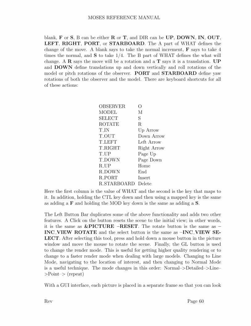
MOSES REFERENCE MANUAL
blank, F or S, B can be either R or T, and DIR can be UP, DOWN, IN, OUT,LEFT, RIGHT, PORT, or STARBOARD. The A part of WHAT defines thechange of the move. A blank says to take the normal increment, F says to take 4times the normal, and S to take 1/4. The B part of WHAT defines the what willchange. A R says the move will be a rotation and a T says it is a translation. UPand DOWN define translations up and down vertically and roll rotations of themodel or pitch rotations of the observer. PORT and STARBOARD define yawrotations of both the observer and the model. There are keyboard shortcuts for allof these actions:
OBSERVER OMODEL MSELECT SROTATE RT IN Up ArrowT OUT Down ArrowT LEFT Left ArrowT RIGHT Right ArrowT UP Page UpT DOWN Page DownR UP HomeR DOWN EndR PORT InsertR STARBOARD Delete
Here the first column is the value of WHAT and the second is the key that maps toit. In addition, holding the CTL key down and then using a mapped key is the sameas adding a F and holding the MOD key down is the same as adding a S.
The Left Button Bar duplicates some of the above functionality and adds two otherfeatures. A Click on the button resets the scene to the initial view; in other words,it is the same as &PICTURE –RESET. The rotate button is the same as –INC VIEW ROTATE and the select button is the same as –INC VIEW SE-LECT. After selecting this tool, press and hold down a mouse button in the picturewindow and move the mouse to rotate the scene. Finally, the GL button is usedto change the render mode. This is useful for getting higher quality rendering or tochange to a faster render mode when dealing with large models. Changing to LineMode, navigating to the location of interest, and then changing to Normal Modeis a useful technique. The mode changes in this order: Normal–>Detailed–>Line–>Point–> (repeat)
With a GUI interface, each picture is placed in a separate frame so that you can look
Rev Page 60

MOSES REFERENCE MANUAL
at them again. If you wish, you can delete some of the frames with the option:
–DELETE, N:M
Where N and M are numbers. With this option, MOSES will delete frames N throughM. If M is omitted, all frames greater than and equal to N will be deleted. If only asingle number is specified, then only that frame will be deleted.
Rev Page 61

MOSES REFERENCE MANUAL
VIII.C Picture Selection
There are quite a few options which can be used to paint only a portion of the dataavailable. They are:
–XG WIND, X MIN, X MAX–YG WIND, Y MIN, Y MAX–ZG WIND, Z MIN, Z MAX–CONNECTORS, :CONE SEL–POINTS, :PNT SEL, D MIN, D MAX–ONE VERTEX, :1V SEL–RATIO, BEG RATIO, END RATIO–STRESS, BEG RATIO, END RATIO–CDR, BEG RATIO, END RATIO–NAMES, :NAME SEL–BODY, :BODY SEL–PART, :PART SEL–PIECE, :PIECE SEL–PARENT, :PART SEL–CATEGORY, :CAT SEL–ENDS, :END SEL(1), ..., :END SEL(4)
The three options –XG WIND, –YG WIND, and –ZG WIND provide the abil-ity to select portions of the model for viewing. MOSES checks the coordinates ofeach element of the picture against a ”window” in space and scales the plot so thatonly those strings which are within the window will be plotted. Here, X MIN andX MAX define the limits of the window in the global X direction. Likewise, Y MINand Y MAX define the window in the global Y direction and Z MIN and Z MAX doso in the global Z direction.
One may select only a portion of the strings for viewing by using some of the remainingoptions listed above. The –CONNECTORS, –POINTS, and –ONE VERTEXoptions define a selector defining the connectors, points, or one vertex elements(strings with a single vertex) which will be plotted. If the selector is @ then allall will be shown, if it is blank, then none will be plotted, etc. The values D MINand D MAX define the minimum and maximum diameter (inches or mm) of theshape used to represent the points. The diameter used will be based on the diameterof the elements in the model. The –POINTS option can be used in conjunctionwith –ANNOTATE POINTS to show specific points in the model.
The –RATIO, –CDR, and –STRESS options selects strings for plotting basedon the value of their ”ratio” ”cdr” or ”stress”. Only strings with a ratio, cdr, orstress between BEG RATIO and END RATIO will be plotted. With the –NAMES,
Rev Page 62

MOSES REFERENCE MANUAL
–BODY, –PART, –PIECE, –PARENT, –CATEGORY, or –ENDS optionsthe selectors: :NAME SEL, :BODY SEL, :PART SEL, :PART SEL, :PIECE SEL,:CAT SEL, and :END SEL(1), ..., :END SEL(4) will select strings based on the valuesof the appropriate quantities associated with the string. To qualify for being in apicture, a string must be selected by all five selection criteria.
Rev Page 63

MOSES REFERENCE MANUAL
VIII.D Picture Special Effects
In addition to the other things, the options
–WATER COLOR, YES/NO–DEFLECT, DFLMAG–ANOTATE, WWHAT–COLOR, CRITERIA–BACK COLOR, YES/NO–CULL BACK, YES/NO–CROP FOR TITLE, YES/NO–SHRINK, AMOUNT–T SIZE, TITLE SIZE–A SIZE, ANO SIZE–WG MIN, SIZE
can be used for special effects. The –WATER COLOR option with a YES/NOof YES will use a different color (slightly darker) for things under the water thanthe color for those above. It will also result in the intersection of a panel with thewaterplane being drawn. A YES/NO of NO will not produce the intersection and alllines of a panel will be drawn in the same color.
The –DEFLECT option instructs MOSES to make a plot of the deflected shapeof the strings. Here, DFLMAG is the magnification which will be applied to thedeflection when making the plot. To return to normal plots, one should use the–DEFLECT option with a magnitude of zero or less.
The –ANOTATE option defines whether or not the strings will be annotated withtext when they are plotted. If WWHAT is NO, no annotation will be made. IfWWHAT is NAMES, the names of the strings will be plotted. If WWHAT isPOINTS, only the names of the points (strings with one vertex) will be plotted.Conversely, if WWHAT is STRINGS, only the names of strings with more than onevertex will be plotted. To plot only class names of strings, one should use PARENT.If WWHAT is RATIO or STRESS, then ratio or stress associated with the stringwill be used for annotation. To plot only the ratio or stress of points, one shoulduse P RATIO or P STRESS. To plot only the ratio or stress of strings with morethan one vertex, one should use S RATIO or S STRESS.
The next set of options control the meaning of the color used for the plot. Bydefault, different strings are assigned different colors based on familial relationships.This mapping of color to string can be altered with the –COLOR option. Here, CRI-TERIA must be either MODELED, BODY, PART, RATIO, CDR, STRESS,FLOODED, or SELECTED. With a value of MODELED the color of a string
Rev Page 64

MOSES REFERENCE MANUAL
is determined by the color defined by either &DEFAULT or the string attributeitself. With values of BODY or PART, the color of a string will be determinedby its body or part. Each string has, as attributes, a ratio, a cdr, and stress, andeach point has a deflection. By specifying RATIO orCDR, a color will be asso-ciated with each string based on the value of its ratio or cdr. Likewise, STRESSassociates a color based on the ratio of the string’s stress to its yield stress. For aCRITERIA of FLOODED or SELECTED the entire picture will be plotted in a”weak” color, while also honoring any window options. For FLOODED the floodedbeams will be plotted in a bright color. Likewise, for SELECTED strings selectedby the –RATIO,–CDR, –NAMES, –BODY, –PART, –PARENT, or –ENDSoptions are then plotted in a bright color. This is an excellent way to identify wherethese selected strings are located in an overall view of a model. Notice that usingSELECTED with an –ANOTATE option and any selection option will yield apicture that only annotates the selected portion yet allows you to see the completepicture.
The option –CULL BACK with a YES/NO of YES will omit the plotting of anypolygon which faces toward the back of the view. Use of this option with a YES/NOof NO will revert to plotting all polygons. The –BACK COLOR option with aYES/NO of YES will use a different color for back facing polygons. Of course, aYES/NO of NO will paint all polygons of the same class in the same color. The–CROP FOR TITLE option allows one to set the upper boundary for a pictureto be below the title if YES/NO is YES. If YES/NO is NO, then the picture will bedrawn over the title.
The –SHRINK option will move the outline of a string inward toward its centeran amount AMOUNT. This is quite useful when using color to select things in amesh model. Without shrinking, the color of a panel can be overwritten by the colorof its neighbor. Also, this option is useful when looking for ”missing” panels or inconjunction with –BACK COLOR when looking for incorrectly ordered panels.The –T SIZE and –A SIZE options allow one to change the size of titles andannotation characters respectively. The defaults are 10 pixels for both.
Finally, the –WG MIN options defines the minimum wave grid size to be ”SIZE”.
Rev Page 65

MOSES REFERENCE MANUAL
VIII.E Picture Animation
Normally, one receives a single picture in response to a &PICTURE command. If,however, this command is issued from either the Static Process Menu or the ProcessPost–Processing Menu, an animation of the process will be plotted. For an animation,the number of frames can be controlled with the option:
–EVENTS, EVE BEGIN, EVE END, EVE INC
Here, EVE BEGIN is the first event for which a picture will be drawn, ESTOP isthe last event for which a picture will be drawn, and EVE INC is the increment atwhich pictures will be drawn between EVE BEGIN and ESTOP. One can specifymultiple sets of these three values, and pictures will be drawn according to each set.By default, all events in the process will be plotted. If this ”goes by too fast”, usethis option with
–EVENTS 0 9000 .1
which plots frames at .1 increments. If this is still too fast, change .1 to somethingsmaller. Of course, increasing the increment will speed up the picture.
If one one has an animation, the option
–MOVIE M TYPE, F RATE, P MULT
will produce a movie. When this option is used, the movie will be written to the a fileand then operation will return to normal. Here, M TYPE is the format of the movieand it must be either: AVI or MPG. F RATE, is the frame rate, and P MULT isthe ”play multiple”. This will result in a movie with frames between EVE BEGINand ESTOP (defined with the –EVENTS option discussed below) at
P MULT / F RATE
second intervals. Notice that if P MULT is .5, then the movie will be played at onehalf of the default speed. The defaults are to use a frame rate of 5, to play the entireprocess, and to use a play multiple of 1. If this is not smooth enough, you may wantto increase the frame rate, but this will increase the time required to generate themovie. Finally, if you use M TYPE of AVI, then Windows Media Player will notplay it unless you have DviX codecs installed.
Rev Page 66
MOSES REFERENCE MANUAL
VIII.F Picture Ray Tracing
For achieving an even higher image quality or generating high resolution images ofyour model, MOSES supports exporting to a ray–tracing program. Ray tracing calcu-lates the path of every beam of light in your scene, making it a very computationallyintensive process, but one that can handle reflections, refraction, and transparencycorrectly, as opposed to the approximations we make in the normal 3D display inorder to give users a smooth, interactive experience.
To export a scene for ray–tracing, it is recommended (but not required) that usersfirst visualize the scene in MOSES’s 3D viewer. Once the scene is positioned correctly,issuing the command:
&PICTURE –RENDER RAYTRACE –SAVE
will generate a file in the .ans directory called povxxxxx.pov which can be loadedand run by POV–Ray by double–clicking on it. If double–clicking on the file doesnot open POV–Ray, you need to download and install it from here The downloadsare about half–way down the page.
Once you have it installed, double–clicking the .pov file should open it. Hit the Runbutton in POV–Ray to begin the render. For better quality, we recommend goingto the menu and selecting ”Render–>Edit Settings/Render” and selecting the lastoption under ”Section:” [1280x1024, AA 0.3].
For those looking for an even more realistic rendering, you can use the &PICTUREoption
–W FANCY YES/NO
This option with YES/NO of YES will render realistic small waves when there is nosea specified.
After installing POV–Ray, command line users can directly operate on the pov00001.povfile by executing something like the following:
povray –ipov00001.pov –w1024 –h768
This would take input file pov00001.pov and render it at 1024x768. For furtheroptions, see the POV–Ray documentation.
Rev Page 67

MOSES REFERENCE MANUAL
IX. ADVANCED LANGUAGE FEATURES
In addition to the basic command structure outlined above, MOSES provides manyfeatures of a programming language. In MOSES, one can alter the flow of eithercommand or description input, make logical checks, define variables, create macros,etc. All of these features operate on both commands and descriptions, so that withthis language, one can automate the definition of a model as well as build a set ofspecific commands he needs to perform repetitive tasks. The language described hereis an interpreted, string based language. In other words, all of the functions describedhere are performed before control is passed to the command interpreter.
Rev Page 68

MOSES REFERENCE MANUAL
IX.A Variables
MOSES has two types of variables, global and local. The difference between the twois the extent of their lives. A global variable lives forever (as long as the database fora given root exists), while a local variable vanishes once the procedure which definedit ceases to exist. The scheme employed here is similar to that used elsewhere in thatif one defines a local variable with the same name as a global one, then the globalvariable will be ”over loaded” as long as the local variable is active. In other words, ifone defines a local variable with the same name as a local variable in a higher macroor with the same name as a global variable, the previous one will not be used so longas the new local variable remains defined. The ”dummy variables” in macros are aspecial case of local variables.
By a variable, we mean a string which is stored in the database and which may bereferred to by its name. Before one may reference a global variable, it must be definedvia a &SET command. The form of this command is:
&SET, VAR, =, value
Notice that the equal sign must be followed by a space or comma before the value.All variables (including arguments) are processed as string replacements. In otherwords, the above command defines a string of characters. These characters will bereplaced whenever the string %VAR is used in an input record. There are actuallyseveral ways of instructing MOSES to substitute a variable. In all cases, the variablemust be referenced with a % as the beginning character. The next character may bea (, in which case, the reference must end with a ). If the ( is omitted, the referencecan end with either a %, a comma or a blank. The only real reason to enclose thename in parentheses is that MOSES will honor one level of recursive use of variables.
For example:
&SET DOG = 20&SET CAT = %DOG%*2000&SET COW = %DOG%A
or
&SET COW = %(DOG)A
Rev Page 69

MOSES REFERENCE MANUAL
&TYPE %COW%
or
&TYPE %COW
or
&TYPE %(COW)
will set variable DOG to 20, CAT to 20*2000 (i.e. 40000), COW to 20A, and willtype 20A to the terminal. For the recursive use of variables, consider:
&SET DOG1 = 20&SET DOG2 = 40&SET INTE = 1&SET ANS = 30*%(DOG%(INTE))&TYPE %ANS
will result in 30*20 being written to the terminal. Here, the variable INTE will beevaluated first, and then the variable DOG1 will be substituted.
Often, one wishes to have variables which are local to a given macro. This can beaccomplished by ”typing” a set of variables to be local as follows:
&LOCAL, LVAR(1), LVAR(2) = VAL, ......
When local variables are typed, their values are set to blank, unless one follows thevariable name with a token of = and another token containing the value to whichthe variable is to be set. Once a local variable is typed, it may be reset via an &SETcommand and used as if it were a global variable.
Rev Page 70
MOSES REFERENCE MANUAL
IX.B Loops and IF’s
Two elements which must exist before a language can be useful are some means ofaltering execution and some method of repetition. Here, the execution control isoffered by a standard block IF construct:
&IF, LPHRASE(1), &THEN&ELSEIF, LPHRASE(2), &THEN&ELSE&ENDIF
Here, LPHRASE(1) and LPHRASE(2) are ”logical phrases”, and if LPHRASE(1)is .TRUE., then the commands which follow will be executed until the &ELSE isencountered. If LPHRASE(1) is .FALSE., then MOSES will evaluate LPHRASE(2).If it is .TRUE., then the commands following &ELSEIF will be executed until&ELSE is encountered, otherwise the commands between &ELSE, and &ENDIFwill be executed. Both &ELSEIF and &ELSE may be omitted, and more than one&ELSEIF can be placed between an &IF and &ELSE, but &IF and &ENDIFmust always be present. There is virtually no limit on the nesting of &IF blocks.
In MOSES, the concept of repetition is implemented via the constructs:
&LOOP, INDEX, BEGVAL, ENDVAL, INCR&LOOP, VAR, ( LIST(1), ...... LIST(n) )&NEXT, LPHRASE&EXIT, LPHRASE&ENDLOOP
The &LOOP command marks the beginning of a set of commands which will berepeated and the &ENDLOOP command marks the end. When this constructis encountered, MOSES will continue to execute the commands delimited until atermination criteria is satisfied. Termination can occur in one of two ways dependingupon the form of the &LOOP command itself. The parameters on the first formof the &LOOP command allow for an ”indexed” loop. In other words, INDEXis the name of a local variable which will be set to the integer BEGVAL at thebeginning of the loop, and it will be updated to its current value plus INCR at eachrepetition. Loops of this type will terminate when INDEX is greater than ENDVAL.The second form of &LOOP is a ”while” on the values in parenthesis. In otherwords, with this form, the variable VAR will be set to the value LIST(1) for the firsttrip through the loop, LIST(2) for the second trip, etc. The loop will terminate afterLIST(n) has been used. Alternately, a loop will terminate whenever an &EXITcommand is encountered with a logical phrase of .TRUE.. The commands betweenthe &LOOP and the &ENDLOOP are executed in order. A ”jump” to the bottom
Rev Page 71

MOSES REFERENCE MANUAL
of a loop occurs whenever an &NEXT command is encountered with a logical phraseof .TRUE.. An example of the first form of the loop command is shown below:
&LOOP I 1 &TOKEN(N %NODES%) 1&SET J = %I%&NEXT &LOGICAL(%J% .EQ. 9)&EXIT &LOGICAL(%I% .GT. 11)&TYPE This is Loop Number %I%
&ENDLOOP
Here, I is the INDEX, and the loop continues from 1 to the number of tokens in thevariable NODES, in increments of 1. The variable J is set to the value of I each passthrough the loop, and a message is typed to the screen. If the J is equal to 9, themessage is not printed. If I is greater than 11, or if I is the number of tokens in thevariable NODES, the loop is terminated.
To terminate execution of either a macro or a command file, one can use the com-mand:
&EOFILE, LPHRASE
When this command is encountered, and LPHRASE is .TRUE., the command file ormacro will terminate execution. Similarly, one can conditionally terminate executionof the program by:
&FINISH, LPHRASE
which terminates the program if LPHRASE is .TRUE..
Rev Page 72
MOSES REFERENCE MANUAL
IX.C Macros
MOSES allows a user to execute a series of commands with the input of a singlename. This is accomplished by allowing the user to define a ”macro”. Macros allowthe user to conditionally execute commands, repeat blocks of commands, and setboth local and global variables. These capabilities provide the user with a true ”highlevel” language in which he can actually write a program to accomplish commontasks.
One defines a macro as follows:
&MACRO, NAME, ARG(1), ARG(2), ..., ARG(n), \–OPTION(1), OPTVAR(1), CARG(1) = DEFAULT(1), ... \–OPTION(2), OPTVAR(2), CARG(2) = DEFAULT(2), ...
COMMAND(1)COMMAND(2)...&ENDMACRO
Here, COMMAND(i) is any command which is either an internal command or avalid program command. The data following &MACRO is called the ”picture” ofthe macro and NAME is the name of the macro and ARG(i) are the valid argumentsto the macro. While there are no restrictions on the names for macros, one shouldbe careful not to choose a name which will conflict with a valid program command.If the valid arguments are specified as above, then MOSES will parse the commandfor you and check for syntax errors. In some cases, however, one neither knows norcares precisely the number or type of the arguments which will be specified. In thiscase, only the macro name should be specified when defining the macro. In all cases,the arguments actually supplied to the macro by the user will be available in thelocal variable ARGV. Thus, one can parse the values himself using &TOKEN andARGV.
The arguments are ”local variables” to the macro. When the macro is invoked (orexecuted), the user defines the values of the variables on the command. In otherwords, to execute the above macro, one would issue the command:
NAME, ARG1, ARG2, ...., ARGn
Now, suppose that for some command in the macro, the user had used the value for
Rev Page 73

MOSES REFERENCE MANUAL
ARG1 which was accomplished by including the line:
COMMAND, %(ARG1)
When the macro is executed, the string %(ARG1) will be replaced by the stringwhich is passed to the macro.
The options in macro arguments allow one to construct macros which have optionalarguments. Any string on the macro definition line which begins with a – is consideredto be a macro option. The string following the option name OPTVAR(i) is the nameof the option variable which is set to .FALSE. if the option is not exercised whenthe macro is executed and to .TRUE. if the option was exercised. The other stringsfollowing an option (ARG(i)) are ”optional data”. The values of the optional dataare all blank if they were not specified when the macro was executed. Additionally,one can specify a default value for this data, using the ” = DEFAULT ” syntax afterthe optional data.
When MOSES parses the picture, it will associate any ”excess tokens” with the lastvariable in the picture. As an example, suppose that a macro was defined as:
&MACRO COW A B –OPT OPT C&ENDMACRO
and that it was executed by:
COW C D E –OPT THIS IS AN OPTION
The results of this would be that the variable OPT would be set to .TRUE., A wouldbe set to C, B would be set to D E, and C would be set to THIS IS AN OPTION.The same result can be obtained through the use of defaults. Consider the followingmacro defined as:
&MACRO COW A = C B = ’D E’ –OPT OPT C = ’THIS IS AN OPTION’&ENDMACRO
and executed by:
COW –OPT
This operation would behave the same as the previous example, but with fewerkeystrokes. Notice the use of the single quotes to delimit data containing blanks.
By definition, a macro will be executed whenever the user specifies the macro name
Rev Page 74

MOSES REFERENCE MANUAL
as a command. One may restrict when a macro can be executed by the followingcommand:
&M ACTIVE, NAME, COMNAM
After this command has been issued, macro NAME will only be executed from menuswhich have COMNAM as a valid command. This command should be used whenone creates a macro containing commands which must be executed from a specificmenu.
Sometimes, one will define a macro with a name which conflicts with a commandname. If this occurs, it can be rectified by changing the name of the macro. This isaccomplished via the &M CNAME command. Its form is:
&M CNAME, OLD NAME, NEW NAME
Also, if one defines a macro which does not work properly and he wishes to changeit, he can delete the macro and start over. This is accomplished as:
&M DELETE, MACRO NAME
Rev Page 75
MOSES REFERENCE MANUAL
IX.D String Functions
Perhaps one of the more useful concepts MOSES employs is the ”String Function.”A string function converts an input string into another string, and the general syntaxof a string function is:
&FUNCTION(ARG(1), ARG(2), ......)
There are quite a few things which can be accomplished with string functions. In thenext several sections specific string functions will be discussed, but some examplesare a string function is o check if a variable has been defined. The function:
&V EXIST(VARNAM)
will return the string, .TRUE. if the variable VARNAM has been defined. If VAR-NAM has not been defined, a value of .FALSE. is returned. Another useful stringfunction is &FORMAT which is used for formatting, and its form is:
&FORMAT(FMT, STRING)
Here FMT is a formatting instruction and STRING is the string to be formatted. IfSTRING is a number, then FMT can be a FORTRAN format (e.g. F10.2, I3, etc.).Otherwise, FMT must be either: UPPER, LOWER, FIRST, or COMMA. ForUPPER, the entire string will be made into upper case characters, and for LOWER,the converse will occur. FIRST transforms only the first character in the string intoupper case. Finally, COMMA adds a comma after each token in the string and an”and” between the last two tokens. FMT can have at most 8 characters.
To compress a logical phrase, one can use the function:
&LOGICAL(LPHRASE)
Here, a logical phrase is a string of numbers, characters, and logical variables com-bined by logical operators. Here, numbers are any string which can be converted to anumber and logical variables are strings with values of either .TRUE. or .FALSE..Any two tokens can be compared by the logical operators: .EQ. and .NE.. For num-bers, four additional operators are available: .LT., .LE., .GT., and .GE.. These sixoperators denote respectively: equal, not equal, less than, less than or equal, greaterthan, and greater than or equal.
A single logical variable can be modified by the operator .NOT., and two logicalvariables can be combined by the two operators .AND. and .OR.. As examples,
Rev Page 76

MOSES REFERENCE MANUAL
consider:
&LOGICAL(A .EQ. A)&LOGICAL(.NOT. A .EQ. A .AND. B .EQ. B)&LOGICAL(5 .LE. 4)&LOGICAL(5 .GT. 4 .OR. A .EQ. B)
The strings resulting from these functions would be respectively: .TRUE., .FALSE.,.FALSE., and .TRUE..
Rev Page 77

MOSES REFERENCE MANUAL
IX.D.1 The &INFO String FunctionOften, one wishes to know the current settings. To accomplish this task, MOSESprovides the string function:
&INFO(NAME, DATA)
In general, there are four classes of information available. Information about:
• Error information,• Run information,• Unit information,• File information,• Program information,• Current output device information, and• Graphics information.
Error information is obtained with a NAME of SEVERITY. When using macros orloops. it is sometimes useful to know if an error or warning occurred during execution.If so, appropriate action can be taken. The string function
&INFO(SEVERITY FLAG)
is used to determine if an error or warning has occurred. Here, FLAG is eitherERROR or WARNING. The function will return a value of .TRUE. if FLAG isset to WARNING, and either an error or a warning occurred during the previouscommand. Likewise, a value of .TRUE. is also returned if FLAG is ERROR, andan error occurred during the previous command. Otherwise, a value of .FALSE. isreturned. Consider the following example:
&IF &INFO(SEVERITY ERROR) &THEN&TYPE LOST BEYOND HOPE&FINISH
&ELSE &INFO(SEVERITY WARNING) &THEN&TYPE FIXING SITUATIONFIXUP
&ENDIF
In this example, a message is typed to the screen and a fixup macro is executedif a warning resulted from the previous command. If an error occurred, a differentmessage is typed, and the program is exited.
Run information is obtained with either: MENU DATE, T OF DAY, TITLE,SUBTITLE, ROOT, or CWD. The first of these returns the current menu while
Rev Page 78

MOSES REFERENCE MANUAL
the second returns the date and the third the twenty four hour time when the functionwas called. TITLE and SUBTITLE return the title and subtitle respectively. ROOTreturns the root file being executed as a file alone and CWD returns the currentworking directory of the program. Thus, to have a fully qualified path name of a filewith the same path and primary name as the root, but with an extension of NEW,one would use:
&INFO(CWD)&INFO(ROOT).NEW
Unit information is obtained with either: BFORCE, LFORCE, BLENGTH, orllength. If BFORCE is used, then a string describing the unit used for ”big force”( kips, l–tons, s–tons, kn, or tonnes) is returned. The other admissible values returnthe names for ”little force” (pounds or newtons), ”big length” (feet or meters), and”little length” (inches or mm ).
File information is obtained with either: C FILE, C PATH, C IFILE, C IPATH,C CFILE, C CPATH, FILE EXISTS, or CHA FILE. Here, C FILE and C PATHreturn the names of the last file and path used by MOSES. C IFILE and C IPATHreturn the last used input file, meaning names ending in .dat and input file path.Types of C CFILE and C CPATH return the last used command file, meaningnames ending .cif and the command file path. FILE EXISTS returns .TRUE. or.FALSE. based on where DATA is a file which exists. CHA FILE returns the filecurrently associated with the channel specified.
Program information is obtained with: VERSION, REVNUM. HOME, PGM-PAT, or OS CLASS. VERSION returns the general version being executed; e.g.REV 5.10, while REVNUM returns the total revision number; e.g. REV 5.10.010.HOME returns the path to the user’s home directory. PGMPAT returns the path towhere the program being executed is stored; e.g. /ultra. A type of OS CLASS willreturn the type of operating system currently running the program.
For information about the current output device, one should use a NAME of either:TPGLEN, OPGLEN, FONT, PWIDTH, PHEIGHT IMARGIN, OMAR-GIN, TMARGIN, BMARGIN, DOUSIDE LPI, CPI, or DEVICE. The DE-VICE value will return the physical device name of the current output device. Alldimensions here returned here are in points except for CPI and LPI which are char-acters per inch and lines per inch respectively. Here TPGLEN returns the length ofthe screen. All of the others provided information about the current output channel.
Information about the current graphics is obtained with either: FIG NUM, orPICT TYPE. FIG NUM, returns the number of the next figure plotted. PICT TYPEreturns the type of data currently being used for pictures.
Rev Page 79

MOSES REFERENCE MANUAL
IX.D.2 The &NUMBER String FunctionPerhaps one of the most useful string functions is the function:
&NUMBER(TYPE, NUM(1), NUM(2), .......)
This function has an option keyword, TYPE, and a set of strings which are normallynumbers. Here, the valid forms of the function are:
&NUMBER(?, STRING)&NUMBER(REAL, RN)&NUMBER(INTEGER, RN)&NUMBER(SIN, RN)&NUMBER(SIND, RN)&NUMBER(COS, RN)&NUMBER(COSD, RN)&NUMBER(TAN, RN)&NUMBER(TAND, RN)&NUMBER(ACOS, RN)&NUMBER(ASIN, RN)&NUMBER(ATAN, RN)&NUMBER(ATAN2, X, Y )&NUMBER(SQRT, RN)&NUMBER(LN, RN)&NUMBER(EXP, RN)&NUMBER(ABS, RN)&NUMBER(MIN, RN(1), RN(2), ...)&NUMBER(MAX, RN(1), RN(2), ...)&NUMBER(MEAN, RN(1), RN(2), ...)&NUMBER(SORT, RN(1), RN(2), ...)&NUMBER(INTERPOLATE, X, X(1), ... Y(n))&NUMBER(NORM, RN(1), RN(2), ...)&NUMBER(DOT, RN(1), RN(2), ...)&NUMBER(UNIT VEC, RN(1), RN(2), ...)&NUMBER(CROSS, RN(1), RN(2), ...)&NUMBER(SCALE, SF, RN(1), ...)&NUMBER(ADDV, SF, RN(1), ...)&NUMBER(3PTS2Q, P1(1), P1(2), ... P3(3))&NUMBER(VECG2L, Q VG(1), VG(2), VG(3) )&NUMBER(VECL2G, Q VL(1), VL(2), VL(3) )
The result produced depends, of course, upon the value of TYPE. The first option,?, is different from the others, in that it returns a value of .TRUE. if the string is a
Rev Page 80

MOSES REFERENCE MANUAL
valid number or .FALSE. if it is not. All of the others return a set of numbers.
As an example of how these functions operate, consider the following:
&NUMBER(REAL, (2+3)**8/2.)
This function will read the string ”(2+3)**8/2.” and convert it to a number, andthen convert this number back into a string with eight significant figures. It is thisfinal string which will be passed to the command interpreter. The function with atype of INTEGER operates in a similar manner, except that here, the result willbe an integer. The idea behind these two is that in some cases a string representinga number may become too long to convert; therefore, strings can be ”compressed”with this function.
The first several TYPEs take a single number as input and return a single number.The particular conversion which occurs with most values of TYPE is rather obviousfrom the name. In particular, SIN, COS, TAN produce strings with the value ofthe trigonometric functions of the same name and with the argument in radians. Thetrigonometric functions which end in D assume that the argument will be in degrees.The functions ATAN, ATAN2, ACOS, and ASIN are inverse trigonometric func-tions, and ATAN2 returns the angle who’s tan is X/Y. The angles returned here are inradians. The types of LN, EXP, SQRT, and ABS produce the natural logarithm,the exponential, the square root, and the absolute value respectively.
The remainder of TYPEs take more than a single number as arguments. The MAXand MIN return the extremes of the arguments. A type of MEAN returns the meanof a set of numbers, while a a type of SORT sorts a set of numbers in ascendingorder. INTERPOLATE takes the first number as the desired ”X” value, the nextN/2 numbers as an array of Xs and the last N/2 numbers as an array of Ys. Itreturns the Y values which corresponds to the first number input. Of course, the Xvalues must be in increasing order.
The next remainder of TYPEs allow one to treat strings as vectors of numbers. For atype of NORM, MOSES will return a string which is the square root of the sum of thesquares of the numerical arguments. For a TYPE of DOT, the number of numericalarguments must be divisible by two, and it returns the inner product of two vectorsrepresented by the 2*n numbers. With UNIT VEC the value returned is the inputvector scaled by its length. With SCALE, the first number is a multiplier and thefunction will return N numbers which represent the remaining numbers multipliedby the first. ADDV takes the first number and uses it as a scalar multiplier for thefirst N/2 numbers and it vectorially adds the result to the second N/2 numbers.
The last three functions deal with matrices and vectors. The TYPE 3PTS2Q returns
Rev Page 81

MOSES REFERENCE MANUAL
a direction cosine matrix. Here P1, P2, and P3 are the coordinates of three points(You need nine numbers here). The ”origin” of the local system is at P1. The vectorfrom P1 to P2 points ”in the direction of the local X axis, and the vector from P1to P3 points in the direction of the local Z axis. This direction cosine matrix willtransform local vectors into global ones. The TYPE VECG2L transforms a vectorin global coordinates to local ones and VECL2G performs the inverse. Here Q isa direction cosine matrix (there are nine numbers for Q) VG is a vector in globalcoordinates and VL is a vector in local coordinates.
Rev Page 82

MOSES REFERENCE MANUAL
IX.D.3 The &STRING String FunctionAnother function for dealing with strings is:
&STRING(ACTION, STRING(1), STRING(2), ..... STRING(n))
Here ACTION defines what you want the function to do, and STRING(i) are thestrings. STRING(1) is the ”basic string” and the others may be used for additionaloperational data, depending on ACTION. Here, the valid forms of the function are:
&STRING(SUBSTR, STRING(1), BCN, ECN)&STRING(BEFORE, STRING(1), DELIM )&STRING(AFTER, STRING(1), DELIM )&STRING(MATCH, STRING(1), STRING(2) )&STRING(NULL, STRING(1) )&STRING(O NUMBER, STRING(1), NUMBER )&STRING(OVERLAY, STRING(1), STRING(2) )&STRING(REVERSE, STRING(1), STRING(2), ..... )&STRING(N EXTRACT, WORD, NUMBER, STRING(3), .... )&STRING(REPEAT, WORD, NUMBER )
For SUBSTR, the result will be the characters BCN through ECN of the inputstring, STRING(1). For BEFORE, the result will be the characters of STRING(1)starting at the beginning of the string through the character before the character DE-LIM. For AFTER, the result is the last portion of STRING(1), beginning with thecharacter after the last occurrence of DELIM. MATCH returns a value of .TRUE.,if STRING(1) matches STRING(2), and .FALSE. if it does not. The functionNULL returns a value of .TRUE. if STRING1 is null, and a value of .FALSE.otherwise. The function O NUMBER ”overlays” the integer, NUMBER, on thestring, STRING(1), starting at the end. For example if STRING(1) is N00000000 andnumber is 3333, then the returned string will be N00003333. The function OVER-LAY works in a similar fashion, except the values here are characters. The command&STRING(OVERLAY 12345678 ABCDE) will return a value of 123ABCDE, for in-stance. Both of these functions are useful for building names, which can be usedto automate the creation of various analytical models. The function REVERSEwill reverse the tokens of STRING1. N EXTRACT will return NUMBER numbersfrom STRING(3), starting at the token immediately following the word WORD. Ifthere are not NUMBER numbers, zeros are returned; i.e. first, WORD is foundin the string, and the next token is checked. If it is not a number or if WORD isnot found, then NUMBER zeros are returned. If this token is a number, then thefirst value returned is set to the number and the next token is checked. This pro-cess is repeated until either NUMBER numbers have been found, or a non–numberterminates the process. Finally, the function REPEAT will return a string with
Rev Page 83

MOSES REFERENCE MANUAL
NUMBER occurrences of STRING.
Rev Page 84

MOSES REFERENCE MANUAL
IX.D.4 The &TOKEN String FunctionOne useful string function is:
&TOKEN(ACTION, STRING2)
which returns a substring of STRING2 based upon ACTION. If ACTION equals L,then the last token of STRING2 is returned, and if ACTION equals N the numberof tokens in STRING2 will be returned. In other cases, ACTION will be a number,a number followed by a :, or a pair of numbers separated by a :. Here, the number,N, will return the Nth token of STRING2, N:M will return Nth through Mth tokensand N: will return the Nth through the last token. If N is greater than the numberof tokens in the string, a null token is returned. For example,
&SET STRING = A B C D E F G H I J K&TYPE &TOKEN(L %STRING )&TYPE &TOKEN(N %STRING )&TYPE &TOKEN(3 %STRING )&TYPE &TOKEN(3:5 %STRING )&TYPE &TOKEN(8: %STRING )
will result in the following being written to the terminal: K, 11, C, C D E, and H IJ K.
Rev Page 85
MOSES REFERENCE MANUAL
IX.D.5 The &GET String FunctionWhen writing macros for MOSES, it is often desirable to prompt the user for infor-mation. This can be accomplished by using the string function:
&GET(WAY, DATA )
This string function returns a string, and here WAY is the manner in which theresponse is obtained and DATA is the other information necessary to make the re-quest. WAY must be either FILE, RESPONSE, YES/NO, PICK, N PICK,GET LIST, or GET NAME and DATA depends upon WAY. The details of howthe information is requested depend on the current user interface. For a terminalinterface, it is all done with text and typing. With a window interface, differentdialog boxes appear.
The first three types of WAY request for a file name, a general string input, and aYES or NO response respectively. Here, DATA is simply a description of the datarequested. For example,
&INSERT &GET(FILE Select your MOSES custom file)
and
&INSERT &GET(RESPONSE Input your MOSES custom file name)
will both return a string, but the first will pop up a file selection box and allow theuser to browse and click on the desired file. The second will pop up an input box andthe string returned may or may not be a valid file name. YES/NO places DATA ina box with YES and NO buttons and returns either YES or NO depending on whichbutton is pushed.
The last four types of WAY pop up a list and the user is allowed to pick from thelist. For PICK the form of DATA is:
MAX PICK, TITLE, ITEM(1), ITEM(2), ....
Here MAX PICK is the maximum number of items which can be chosen, TITLE isthe title of the dialog box, and ITEM(i) are the items which can be chosen. If more
Rev Page 86

MOSES REFERENCE MANUAL
than one item is chosen the string will be composed of the name of each item chosen.
The type of WAY of N PICK stands for ”name pick” and here the form of DATA is:
MAX TO PICK, TYPE OF NAME, TITLE
Here TYPE OF NAME is a valid value of the &NAMES command (issue the com-mand &NAME NAMES to see what is available or see the documentation for &NAMES),TITLE is again the title of the pick box, and MAX TO PICK is the maximum num-ber of items which may be chosen. With this type, the list depends on the currentstate of MOSES, in that the list is obtained from the current database. This removesthe macro writer from having to know the state. As an example, consider
&REP SELECT –BODY &GET(N PICK 1 BODIES ’Select A Body’)
which will present the user with a list of the bodies defined and ask him to selectone.
The last two types of WAY GET LIST and GET NAME have a form of DATA exactlythe same as PICK and N PICK respectively. The difference is that with these types,a combination EDIT/PICK box is popped up. Here one can type data into the editbox or select from the available list, or do both.
Rev Page 87

MOSES REFERENCE MANUAL
IX.E Getting User Input
On can use the &GET string function to simply get a response from the user, butfor many situations this leads to a boring, modal dialogs. A more flexible methodis using &STRING macros and WIZARDS. A wizard is a set of commands whichare defined inside a &STRING macro and A &STRING macro is the same as anordinary macro except that it can contain only internal commands, and it can beexecuted only with an &E STRING command. Let us look at an example, supposethat one wanted to have a command which prompts for the units to use. This canbe accomplished with
&STRING D2M&DIMEN –DIMEN &GET(PICK 1 ’PICK UNITS’ \
’Feet,Kips ’ \’Feet,S–tons ’ \’Feet,L–tons ’ \’Meters,Tonnes’ \’Meters,KN ’ )
END&ENDSTRING&E STRING D2M
Notice that there is an ”END” command at the bottom of the definition of the&STRING macro D2M. This command signals the end of the execution of the macro.At first glance this looks like a concept which is of no value of all, but this is nottrue. First, as we will see later, &STRING macros can be associated with buttonson the menu bar. Also, WIZARDS must be defined with a &STRING macro. Forexample, the above could be accomplished with a WIZARD as:
&STRING D2MWIZARD Dimensions –COMMAND &DIMENSION –SIZE 450 410
TAB ADD To UseWIDGET ADD YES–NO –REMEMBER ”Remember Previous”WIDGET ADD YES–NO –SAVE ”Save Current”WIDGET ADD RADIO –DIMEN ”Settings” \
”Feet, Kips ” \”Feet, L–tons ” \”Feet, S–tons ” \”Meters, Tonnes ” \”Meters, KN ”
END&ENDSTRING
Rev Page 88

MOSES REFERENCE MANUAL
&E STRING D2M
Basically what happens here is the the wizard will build a command from the user’sactions. The beginning of the command will be &DIMENSION and this is definedwith the –COMMAND option. This wizard has one tab labeled ”To Use” (all wizardsmust have a tab) and three things one can choose: two check boxes and one pick froma set of ”radio buttons”. A WIDGET command defines a single widget which willbe placed in the tab and the first token after WIDGET defines the type of widget.The second token defines a prefix which will be added before the main data selectedby the widget. The fourth token is a title The YES–NO widgets select whether ofnot the prefix is added to the command and the RADIO widget will add on of theprefix –DIMEN and the text selected.
Now, let’s be more precise. The command
WIZARD Main Title –OPTIONS
instructs MOSES to enter the Wizard Menu and the options available here are:
–COMMAND First Part of Command–SIZE SHOR, SVER, NCOL–BUTTON TEXT Text On Button
Here, the –COMMAND option was discussed above, and the –SIZE allows theuser to specify the horizontal and vertical size of the wizard window in pixels, andthe number of columns. Every wizard has a button that the user must push to exitthe wizard and execute the command. The –BUTTON TEXT option defines thetext on the button. If this option is omitted, ”OK” will be used.
As mentioned above, every wizard must have at least on tab, and it can have manyof them. Each one is defined with the command
TAB ADD STRING
where ”STRING” defines the text which will be painted on the top of the tab. Oncea tab has been defined, all text and widgets defined will be added to the tab until anew TAB ADD command is issued. The command
TEXT ADD TEXT
will simply add the text ”TEXT” to the current tab and the current location.
Rev Page 89
MOSES REFERENCE MANUAL
WIDGET ADD WIDGET TYPE, W PREFIX, W DESC, W LIST, –OPTIONS
and the available options are
–INITIALIZE W INITIAL VALUE–SUFFIX W SUFFIX–L DESCRIPTION L DESCRIPTION–ACTIVATE KEY TO
Here, WIDGET TYPE defines the type of widget which will be created and it must bechosen from either YES–NO, BOX, RADIO, SEL ONE, or SEL MULTIPLE.The YES–NO widget has a check box. If it is checked, then the prefix will be emitted,if it is not checked, then the prefix will not be emitted. The BOX widget has an inputbox in which the user can put input. If he enters data, then it and the prefix will beomitted. The RADIO widget has a list with a circle. If one clicks on the circle, thethe text shown will be emitted with the prefix. Only a single value can be selected.The SEL ONE and SEL MULTIPLE widgets are drop down selection boxed. Onlya single item can be selected with a SEL ONE widget, but multiple ones can beselected with SEL MULTIPLE. W PREFIX defines the prefix which will be emittedwhen the user selects the widget. It can be blank. W DESC is the brief text whichwill be placed to the left of the selection part of the widget, and W LIST is a list ofthings which can be selected. The text defined here is what will be emitted after theprefix. The order in which widget results are emitted is the order in which they wereinput. Thus, if you use things without a prefix, they probably should be defined first.
The –INITIALIZE and –SUFFIX options defines initial values and suffixes forthe widget. If an initial value is specified, then this will be the value displayed in thebox as if the user input it. A suffix will not normally be needed, but if it is specified,then what is emitted by this widget will be the concatenation of the prefix, the value,and the suffix.
Ideally the words in the list should suffice to tell the user what he is selecting. Some-time this is not the case and you need to add a –L DESCRIPTION option whichdefines a ”long description. This description is written in a pop up window when on”mouses over” the description.
The –ACTIVATE option is complicated. When this option is used, the widget isinitially hidden. Here KEY TO is an option on the previous widget and when theprevious widget selects KEY TO, the hidden widget is shown giving choices whichonly make sense for the chosen value. For example:
WIDGET BOX –DEFLECTION ”Show Deflected Shape” YES NO
Rev Page 90

MOSES REFERENCE MANUAL
WIDGET BOX –DEFLECTION ”Deflection Multiplier” –ACTIVATE YES
Here, the second widget is hidden unless YES is selected by the first one.
Rev Page 91

MOSES REFERENCE MANUAL
IX.F Programming the Tool Bar
The MOSES Tool Bar is a set of buttons at the top of the display area which,when pushed, drop down another set of buttons. Each of these buttons representeither another drop down set of buttons, or a command. The entire system is userprogrammable with a command and ”STRING” macros. The basic command hereis:
&MENU, ACTION, NAME, TITLE(1), RETURN(1), ...
Here, ACTION is the action which must be either CREATE, DELETE, or ADD,NAME is the name of the menu, RETURN is the ”return string”. Of course, the lasttwo items are required for each line in the menu.
The NAMEs associated with menus are up to the user except the one T BAR whichis the name of the Tool Bar itself. Normally the only action one needs is CREATE,but with T BAR, one can ADD a menu to it, or DELETE one he has added. TheTITLE(i) are the strings which are printed on the buttons. For the Tool Bar itself,these are best left short as the real estate is limited. Remember here if you havespaces in any thing, you need to enclose them in either ” or ’ pairs.
Now, RETURN(i) can be either: the name of another menu, the name of a &STRINGmacro, or a true return string. Let us look at an example. Suppose that one wantedto add a button to the Tool Bar to set the dimensions to meters. This can beaccomplished with
&MENU, ADD , T BAR DIM2M ’&DIMEN –D METERS TONNES’
Now, when you push this button, the dimensions will be changed to meters andtonnes. Suppose, however, that you sometimes wish to use kilo–newtons? To allowfor this, you must interact with the user and a &STRING macro is required. Thefollowing:
&STRING D2M&DIMEN –D METERS &GET(PICK 1 ’FORCE UNIT’ TONNES KN)END
&ENDSTRING&MENU ADD T BAR DIM2M D2M
Now, when one pushes the DIM2M button, it will execute the &STRING macroD2M. In here, the user is asked to choose the force unit he wants to use.
The entire Tool Bar structure used in MOSES can be investigated in the file /ul-
Rev Page 92

MOSES REFERENCE MANUAL
tra/data/progm/moses.mac.
Rev Page 93

MOSES REFERENCE MANUAL
IX.G Using Files
Normally the user does not have to worry about the files that MOSES is using. Insome circumstances, however, the user wants to change the file associated with a giventype or to write information to a file of his choice. These things can be accomplishedwith the string function
&F READ(TYPE VAR)
and command
&FILE, ACTION, DATA, –OPTIONS
The string function &F READ is used to read a file and the command &FILEis used for a variety of tasks. When reading or writing, files are referred by typeand TYPE is this type. A TYPE is associated with a file when the file is opened.The string function will read a record from the file and store it in the variable VAR.The value returned by the function is .TRUE. if there is no more data to read and.FALSE. if there is more to read. To check to see if a file exists, you can use thestring function:
&INFO(FILE EXISTS filename)
which returns TRUE if the file exists or FALSE if it does not.
With &FILE the DATA and –OPTIONS depend on the value of ACTION, and thevalid values of ACTION are: MKDIR, RM, MV, CP, USE, ANS DIRECTORY,OPEN, CLOSE, and WRITE. The first four ACTIONS do not have any options:
&FILE MKDIR, A&FILE RM, A&FILE MV, A, B&FILE CP, A, B
where the MKDIR ACTION creates the directory A, the RM ACTION deletes thefile A, the MV ACTION renames file A to B, and the CP ACTION copies file A toB.
The USE action is used to alter the default association of files and file TYPES. Thesyntax here is:
&FILE, USE, TYPE, FILE NAME
and TYPE is the type of file which will be altered. It is a either a user defined file
Rev Page 94
MOSES REFERENCE MANUAL
type or type ”PREFIX” of a channel. Also, FILE NAME is the new file name whichwill be associated with the file type. When this option is exercised, the old file willbe closed and the new one used until further notice.
The ANS DIRECTORY action is used to alter the default association of files andfile TYPES. The syntax here is:
&FILE, ANS DIRECTORY, DIR
where DIR is a directory in which the ”answers” will be stored.
Before one can write to a file, it must be opened with the command:
&FILE, OPEN, –TYPE, TYPE, –NAME, FILE NAME
Here, TYPE is a handle you can associate with the file and FILE NAME is the nameof the file. The handle can be any name of up to eight characters and is used to read,write and close the file. Once a file has been opened, you can write to it with thecommand:
&FILE, WRITE, TYPE, STRING
which writes the line STRING to the file with type of TYPE. After writing a file,you should close it with
&FILE, CLOSE, TYPE, –OPTIONS
If you specify –DELETE then the file will be deleted.
You cannot read and write to a file at the same time. Instead it must be written,closed, reopened, and then read. As an example, consider
&FILE OPEN –TYPE COW –NAME MILK COWS&FILE WRITE COW Brown&FILE WRITE COW Black and White&FILE WRITE COW Holstein&FILE CLOSE COW&FILE OPEN –TYPE COW –NAME MILK COWS&LOOP
&EXIT &F READ(COW VAR)&TYPE %VAR
&ENDLOOP
Rev Page 95

MOSES REFERENCE MANUAL
&FILE CLOSE COW
which writes three lines to a file named MILK COWS and then reads them.
Rev Page 96

MOSES REFERENCE MANUAL
IX.H Functions
While one can accomplish almost anything with the tools that have been discussedpreviously, one finds that if this is all he has, then things get convoluted quickly.MOSES has a concept called ”functions” which can be used to organize data moreeffectively. This concept is based on the true mathematical definition of a function.Suppose that A and B are two sets, and for each element of A there is associated anelement of B. This association of elements is called a function from A to B. The set Ais called the domain of the function, the set B is called the range of the function, andthe elements in B are called the values of the function. What we are going to discusshere are functions who’s domain is either the set of positive integers or a ”variable”and the range of these functions is a set of strings.
In this sense, a ”variable” is not a simple global or local variable. It is, in fact, a setof names, and a name is a string of up to eight characters. The variable itself hasa name which is a string of up to twenty four characters. The name must be of theform
<DBFILE>VAR NAME
Here DBFILE is the name of the database file where the variable will be stored.Now,we could spend a good bit of time talking about this, but lets just say thatthere are two that are always available: MACDBF and SYSDBF, so you should useone of these (preferably MACDBF). VAR NAME is simply the name of the variable.To create a variable, one uses the internal command:
&VARIABLE, VAR NAME, –ADD NAME
Which adds the name ”NAME” to the variable VAR NAME. Now, once a variablehas names, you can find out what they are with the string function
&VARIABLE(–WHILE VAR NAME SEL WHAT )
extracts all the names in ”VAR NAME” that match SEL and sets the (normal globalor local) variable WHAT to the value of the name. It also returns a string .FALSE.if there are more names to be output or .TRUE. if it is finished.
Let’s look at an example:
&VARIABLE <MACDBF>COWS –ADD JERSEY&VARIABLE <MACDBF>COWS –ADD HOLSTEIN&VARIABLE <MACDBF>COWS –ADD ANGUS
Will build a variable <MACDBF>COWS which has three names in it: JERSEY,
Rev Page 97
MOSES REFERENCE MANUAL
HOLSTEIN, and ANGUS. Here we will be using the command &LOOP without anyentries. This advanced method of using &LOOP creates an infinite loop. Now,
&LOCAL LIST =&LOOP
&EXIT &VARIABLE(–WHILE <MACDBF>COWS @ A COW)&SET LIST = %LIST %A COW
&ENDLOOP
will produce the local variable ”LIST” which contains the three names of cows. Fi-nally, there is the string function
&NUMVAR(VAR NAME)
that returns the number of names in the variable ”VAR NAME”; e.g.
&NUMVAR(<MACDBF>COWS)
will return 3.
Often one wishes to ”while” items which are in the database. This can be accom-plished with
&LOOP N ( &NAMES(NODES) )&ENDLOOP
Unfortunately, for large models, this will produce a ”buffer overflow”. When thishappens you need to change the above to
&SET NOD VAR = &NAMES(NODES –V)&LOOP
&EXIT &VARIABLE(–WHILE %NODE VAR @ A COW)&ENDLOOP
The first line above uses the &NAMES string function and the option –V to get thenames that MOSES uses to store the data which allows} you to use the MOSES datadirectly.
As mentioned above, ”functions” are build on top of variables. Before one can addvalues to a function, he must first ”define” it with the internal command:
Rev Page 98
MOSES REFERENCE MANUAL
&DEFINE, FUNNAM, –OPTIONS
Here, FUNNAM is the name of the function, and the available options are:
–DOMAIN, DOMNAM,–MEMORY
Here FUNNAM is the name of the function and it follows the same rules as thosefor a variable name. DOMNAM define the domain of the function. If the option–DOMAIN is omitted, then the domain of the function will be the set of positiveintegers otherwise it is the variable DOMNAM. The option –MEMORY instructsMOSES that the primary residence for values of the function will be in memoryrather than on a file. If omitted, the primary residence will be on the database file.Normally, memory resident functions are accessed more quickly, but not always.
Once a function has been defined you should define its values. This is accomplishedwith the internal command:
&FVPUT, FUNNAM, VAR, STRING
Here, FUNNAM is the name of the function, VAR is the value (name) in the variableDOMAIN associated with STRING. For example:
&DEFINE <MACDBF>COW DATA –DOMAIN <MACDBF>COWS&FVPUT <MACDBF>COW DATA JERSEY Milk&FVPUT <MACDBF>COW DATA HOLSTEIN Milk&FVPUT <MACDBF>COW DATA ANGUS Beef
defines the function <MACDBF>COW DATA and associates data for three typesof cows. To get the values from a function, one uses the string function
&FVGET(FUNNAM, VAR)
The following
&LOOP&EXIT &VARIABLE(–WHILE <MACDBF>COWS @ A COW)
&TYPE The %A COW cow is a &FVGET(<MACDBF>COW DATA %A COW).&ENDLOOP
Will type a line defining the class for each type of cow.
Functions are similar to files. You open and close files but you &READY and &SUS-
Rev Page 99
MOSES REFERENCE MANUAL
PEND functions. The internal command
&READY, FUNNAM
makes the function FUNNAM available for extracting values. When you are throughwith a function, you can use the internal command:
&SUSPEND, FUNNAM, –OPTIONS
The options must be either: –DISCARD, –SAVE, or –CLOSE. If the function isdiscarded when it is suspended, all data for the function is deleted from memory. Ifthe –SAVE option is used, all data for the function will be written to the data basefile if it has changed and the function will remain active. If the –CLOSE option isused, then the function will first be saved and then discarded. In both the subroutinecall and the internal command, FUNNAM can include wild characters. Thus, onecan suspend more than one function with one command.
One thing to know is that at the end of an INMODEL, MOSES closes all function(yours included). Thus you may need to &READY you functions. Actually MOSESfunction are more general that what we have discussed, but this is all that is availablefrom the command interface.
Rev Page 100

MOSES REFERENCE MANUAL
X. THE DISPOSITION MENU
At the conclusion of many commands, the user is placed into the ”Disposition Menu”.In this menu, data may be processed and written to either an output file, a post–processing file, the terminal, a graphics device, or to a global variable.
When dealing with data in the Disposition Menu, it is best to think of it as beinga matrix. The columns of the matrix are called variables and the rows are calledrecords. Each variable is identified by its column number or name , and one canobtain a list of the names of the variables and their column numbers by issuing thecommand,
VLIST.
Throughout this menu, one selects columns with column selectors. These selectorscan be a single number, a colon separated pair of numbers, or a name selector; e.g.5, 7:8, @x:@. The colon pair selects all columns from the first number to the secondone. In many cases, only a limited number of columns can be selected. In this case,the first one selected will be used. For example, suppose that you can select six valuesand you use 1:12 for the column selector, then only 1:6 will be used.
Sometimes, one may wish to alter the values of the data available. This can beaccomplished by using either of the commands:
C SCALE, SCALE F, CS(1), CS(2), ...C SHIFT, SHIRT F, CS(1), CS(2), ...
The C SCALE command defines a multiplier by which a variable will be scaled,and the C SHIFT defines a constant which will be added to the variable. Once ofthese factors are established, they will stay in effect until it is changed with a newC SCALE or C SHIFT command, or until the Disposition Menu is exited.
Rev Page 101

MOSES REFERENCE MANUAL
X.A Reporting, Viewing and Storing Data
Three commands are available which allow one to select portions of the data andwrite it to a post–processing file, an output file, or to the screen.
There are several options which can be used on more than one command:
–HARD–BOTH–HEADING, HEAD–RECORD, BEG RNUM, END RNUM–VALUES, CV, VAL MIN, VAL MAX–MAG USE–FIGURES, COL SEL, RIGHT
They will be defined here and then listed for the commands for which they areapplicable.
By default, the results for commands that produce reports (except for the REPORTcommand discussed above) is to write the results to the terminal. The –HARDoption instructs MOSES to produce a report on the OUTPUT channel and the –BOTH option writes the results to both the OUTPUT channel and the terminal.When these reports are written, they have a single line generic heading. The –HEADING allows one to replace the generic heading with one you specify. You canspecify as many of these options as you wish. The will appear on the page in theorder you specify them.
The –RECORD and –VALUES options defines the records which will be con-sidered. Here, a ”RECORD” is simply a row of the matrix of data. With the –RECORD option the beginning and end record numbers are simply specified. With–VALUES the records considered are defined with the values of a column of data.Here CV is the column number for which the values will be obtained and VAL MINand VAL MAX are two numbers (VAL MIN is less than VAL MAX). BEG REC isthen the largest record number which the values of column CV is less than or equalVAL MIN and END REC is the greatest record number where the value of this col-umn is greater than VAL MAX. If neither –VALUES nor –RECORD are specified,all records will be considered.
The –MAG USE option instructs MOSES to add a second heading line based on thedefinition of magnitude defined with the –MAG DEFINE option. The –FIGURESoption offers a way to change the display of the numbers. It says to change thenumber of figures after the decimal point for columns selected by COL SEL to be
Rev Page 102

MOSES REFERENCE MANUAL
RIGHT figures. You can specify more that one –FIGURES option.
Perhaps the easiest command to explain is the REPORT command, which producesa formatted output file report. The format of this command is:
REPORT, DATA, –OPTIONS
The form of the REPORT command depends upon the original command thatplaced the user here. Often only REPORT is necessary. Some original commandsallow for data and options to be specified on the REPORT command. These detailswill be discussed with the original command.
The next of these is:
VIEW, CS(1), CS(2), ..... –OPTIONS
and the available options are:
–HARD–BOTH–HEADING, HEAD–RECORD, BEG RNUM, END RNUM–VALUES, CV, VAL MIN, VAL MAX–MAG USE
This command offers the user the opportunity to view the selected data at the termi-nal, or, if the –HARD option is specified, the results will be written to the outputfile. The data viewed is defined by the column selectors CS(1), CS(2),.. If no columnselectors are specified, MOSES will prompt the user for all required data.
The STORE command is used to store the selected data in a ”table”. The resulthere is much the same as what you get in the &TABLE menu, i.e. either a CSV orHTML table. The format of the command is:
STORE, CS(1), CS(2), ..... –OPTIONS
and the available options are:
–HEADING, HEAD–RECORD, BEG RNUM, END RNUM–VALUES, CV, VAL MIN, VAL MAX–MAG USE–TITLE, NCOL(1), CT(1), .... NCOL(n), CT(n)
Rev Page 103

MOSES REFERENCE MANUAL
–H SKIP, YES NO–BOLD, YES NO–ROW SHADE, YES NO–EXTR SHADE, COL SEL(1), COL SEL(2), .....–V LINES, COL SEL(1), COL SEL(2), .....
with the exception of –RECORD and –MAG USE these option work exactly asdocumented with &TABLE.
Rev Page 104

MOSES REFERENCE MANUAL
X.B Adding Columns
Occasionally, it is desirable to create a new column of data based on the existingcolumns, or create a completely new column of data. This can be performed withthe command:
ADD COLUMN, NAME, –OPTIONS
where the available options are:
–COLUMN, C(1), C(2), ..... C(n)–INPUT, CS, X(1), Y(1), X(2), Y(2), .....–COMBINE, CS(1), F(1), CS(2), F(2), .....–NORM, CS, NCOL–RMS, CS(1), CS(2), .....–POWER, P N, P C, CS(1), F(1), CS(2), F(2), .....–DERIVATIVE, CS(1), CS(2)–INTEGRAL, CS(1), CS(2)–FILTER, R TYPE CS(1), CS(2), RL(1), RU(1), ... RL(n), RU(n)–SMOOTH, CS, NL, NR, ORDER
The first two options create completely new columns. The –COLUMN option allowsthe user to simply input a column of data. Here, the number of values input mustbe the same as the number of rows of the existing columns. A good source of thisdata may be from SET VARIABLE –COLUMN. On the other hand, the –INPUToption allows more flexibility in the number of points input. Here, CS is the columnselector of an existing column which is ”like” the X values. For instance, if the Xvalues are times, then CS should be the column selector for event number. MOSESwill fit a spline to the input data and then create the new column by interpolating avalue from the spline for every value of CS(i).
The remainder of the options create a column based on the values of the existingones. The –COMBINE option will combine two or more columns of data, using thefactors specified. For instance,
ADD COLUMN NEW –COMBINE 1 1 2 –1
will make the new column the difference of columns of 1 and 2. Here, CS selects thecolumn, and F is the combine factor. To find the norm of two or more columns, the–NORM option is used. CS again selects the column, and NCOL is the number of
Rev Page 105
MOSES REFERENCE MANUAL
columns to consider, including the first one. The command:
ADD COLUMN NEW –NORM 3 3
will find the norm of columns 3, 4 and 5. The –RMS option is similar to –NORM,except that here, one specified the columns to be combined directly. factor. The–POWER option is a generalization of the above. Here, P C is the power eachcolumn is raised before summing and P N is the power to which the sum will beraised; e.g.
ADD COLUMN NEW –POWER .5 2 3 1 4 1 5 1
Gives the same result as the –NORM example and
ADD COLUMN NEW –POWER 1 1 3 3
Gives the same result as the –COMBINE example.
The –DERIVATIVE and –INTEGRAL adds new columns which are the deriva-tive or integral of column CS(2) with respect to column CS(1), and the –LN and–EXP options add columns which are the natural log and the exponential of theoriginal column.
The –FILTER option filters a column of temporal data using a Fourier Transform.Here, R TYPE defines the type of ranges to be input, FREQUENCY for angularfrequency, or PERIOD for periods. MOSES will then compute the Fourier Trans-form of the function with domain in column CS(1) and range in column CS(2). Afterthe transform, all values within any of the ranges defined will be discarded and aninverse transform will be computed for the new column. For example,
ADD COLUMN NEW –FILTER PERIOD 1 4 0 30
will produce a new column named NEW from the old curve defined by columns 1 and4. Here, column 1 is TIME or EVENT. All of the contribution from periods between0 and 30 will be discarded to form the new function.
The –SMOOTH option creates a new column by smoothing an old one, but here,a Savitzky–Golay filter accomplishes the smoothing. CS defines the column to besmoothed, and NL, NR, and M define the smoother. NL is the number of pointsto the left, NR is the number of points to the right and ORDER is the order ofpolynomial used in constructing the filter. The defaults are 8 for NL and NR and4 for ORDER. Since this algorithm does not use Fourier analysis, it can be used to
Rev Page 106

MOSES REFERENCE MANUAL
smooth spectral or FFT data.
Rev Page 107

MOSES REFERENCE MANUAL
X.C Recasting Data
There are three special commands in this menu: SPECTRUM, FFT and CULL.All of these commands take a subset of the original data and transform it into a newset of data to be disposed. This has the interesting effect of one being in the Dis-position Menu from the Disposition Menu. The first time and END is encountered,one leaves the latest Disposition Menu, but is still in the Disposition Menu. Now,however, the original data is again available.
There are several options which can be used on more than one command:
–RECORD, BEG RNUM, END RNUM–VALUES, CV, VAL MIN, VAL MAX
The –RECORD and –VALUES options defines the records which will be con-sidered. Here, a ”RECORD” is simply a row of the matrix of data. With the –RECORD option the beginning and end record numbers are simply specified. With–VALUES the records considered are defined with the values of a column of data.Here CV is the column number for which the values will be obtained and VAL MINand VAL MAX are two numbers (VAL MIN is less than VAL MAX). BEG REC isthen the largest record number which the values of column CV is less than or equalVAL MIN and END REC is the greatest record number where the value of this col-umn is greater than VAL MAX. If neither –VALUES nor –RECORD are specified,all records will be considered.
The form of the first of these commands is:
SPECTRUM, CS(1), CS(2), ..... –OPTIONS
and the available options are:
–RECORD, BEG RNUM, END RNUM–VALUES, CV, VAL MIN, VAL MAX
When issued, MOSES will compute a spectrum for the columns selected by CS(2),.... CS(N), assuming that CS(1) is the independent variable. The form of the secondone is:
FFT, CS(1), CS(2), ..... –OPTIONS
and the available options are:
–RECORD, BEG RNUM, END RNUM
Rev Page 108

MOSES REFERENCE MANUAL
–VALUES, CV, VAL MIN, VAL MAX
These two commands are very similar, the only difference is that with FFT, a Fouriertransform of the data is produced instead of a spectrum. The last of these specialcommands is:
CULL, CS, EXL(1), EXU(1), .... EXL(n), EXU(n)
This command creates a new set of data from the original by excluding specifiedparts. Here, CS defines a column, and other values define ranges of values of theselected column which will be excluded in the new data. For example, consider:
CULL, 1, 0 50 200 300
The new data will contain all of the original except those rows where column 1 hadvalues either between 0 and 50 or 200 and 300. One obvious use for this commandis to extract starting transients from a time sample. Another use is to partitionfrequency domain data to compute independent statistics on each part.
Rev Page 109

MOSES REFERENCE MANUAL
X.D Extremes and Statistics
There are several options which can be used on more than one command:
–HARD–BOTH–HEADING, HEAD–RECORD, BEG RNUM, END RNUM–VALUES, CV, VAL MIN, VAL MAX–MAG USE
They will be defined here and then listed for the commands for which they areapplicable.
By default, the results for commands that produce reports (except for the REPORTcommand discussed above) is to write the results to the terminal. The –HARDoption instructs MOSES to produce a report on the OUTPUT channel and the –BOTH option writes the results to both the OUTPUT channel and the terminal.When these reports are written, they have a single line generic heading. The –HEADING allows one to replace the generic heading with one you specify. You canspecify as many of these options as you wish. The will appear on the page in theorder you specify them.
The –RECORD and –VALUES options defines the records which will be con-sidered. Here, a ”RECORD” is simply a row of the matrix of data. With the –RECORD option the beginning and end record numbers are simply specified. With–VALUES the records considered are defined with the values of a column of data.Here CV is the column number for which the values will be obtained and VAL MINand VAL MAX are two numbers (VAL MIN is less than VAL MAX). BEG REC isthen the largest record number which the values of column CV is less than or equalVAL MIN and END REC is the greatest record number where the value of this col-umn is greater than VAL MAX. If neither –VALUES nor –RECORD are specified,all records will be considered.
The –MAG USE option instructs MOSES to add a second heading line based onthe definition of magnitude defined with the –MAG DEFINE option.
The EXTREME command offers the user the opportunity of obtaining a report onthe extremes of the data. The form of this command is:
Rev Page 110
MOSES REFERENCE MANUAL
EXTREME, CS(1), CS(2), ..... –OPTIONS
and the available options are:
–HARD–BOTH–HEADING, ”HEAD(1)”, ”HEAD(2)”–RECORD, BEG RNUM, END RNUM–VALUES, CV, VAL MIN, VAL MAX–MAG USE
With this command, one will obtain a report of the extremes of the data selected.Here, the first value entered will become the ”independent” variable, and the remain-der the dependent ones. MOSES will search through the results from BEG RNUM toEND RNUM to find the minimum and maximum value of each type of data selected.It will then issue a report for each value of the independent variable at which anextreme occurred. This report will contain the values of all of the variables and aremark as to which variables have suffered an extreme. The report will be written tothe terminal unless the –HARD option was used, in which case it will be written tothe output file.
The STATISTIC command generates a report on the statistics of the data. Itproduces statistics for the results from BEG RNUM to END RNUM for each typeof data selected. The specific form of this command is:
STATISTIC, CS(1), CS(2), ..... –OPTIONS
and the available options are:
–HARD–BOTH–RECORD, BEG RNUM, END RNUM–VALUES, CV, VAL MIN, VAL MAX–MAG USE–HEADING, ”HEAD(1)”, ”HEAD(2)”–TYPE, STYPE–EXTREMES, TIME, DEVIATION, MULTIPLIER
Where the report is written depends on the use of the –HARD and –BOTH options.Here, CS(1) is the independent variable against which the statistics will be computed.Normally, it is ”event” so that the remaining columns of data can be considered to
Rev Page 111

MOSES REFERENCE MANUAL
be time samples. If this is the case, MOSES will compute the following quantities:
MeanVarianceRMSStd. DeviationSkewnessKurtosisAv of 1/3 HighestAv of 1/3 LowestAv of 1/100 HighestAv of 1/100 LowestAv of 1/1000 HighestAv of 1/1000 LowestMaximumMinimumPred. MaxPred. MinAv of 1/3 Highest–MeanAv of 1/3 Lowest–MeanAv of 1/100 Highest–MeanAv of 1/100 Lowest–MeanAv of 1/1000 Highest–MeanAv of 1/1000 Lowest–MeanMaximum – MeanMinimum – MeanPred. Max – MeanPred. Min – Mean
of the variables selected. These quantities are calculated for the It will also computeaverages for the peaks encountered. Notice these peaks are computed from the sam-ples themselves and not by assuming any type of probability distribution. Extremevalues of the maximum and minimum are also predicted. This prediction is controlledby the –EXTREMES option. Here TIME is the time in seconds for the extreme. If,for example, TIME is 3600, then the predicted value will be the probable maximumin one hour. The default is three hours.
In general, the predicted extreme is of the form
PE = MEAN +– DEVIAT * FACTOR
here MEAN is the mean and the plus is used for the maximum and the minus for theminimum. Traditionally, the standard deviation is used for DEVIAT and FACTOR
Rev Page 112
MOSES REFERENCE MANUAL
is given by
FACTOR = sqrt { 2 Log ( r * Np ) }
where Np is the number of peaks in the sample, and r is the ratio of the length ofthe sample to TIME. The values of DEVIATION and MULTIPLIER can be usedto change this behavior. In particular, the value of DEVIATION is used to changeDEVIAT. Here, a value of STANDARD will use the standard deviation while avalue of PEAKS will use the largest peak and smallest peak values minus the mean.PEAKS is the default and normally gives better predictions than the traditionalmethod. The final value, MULTIPLIER can be either GAUSSIAN or WINTER-STEIN. GAUSSIAN is the default. If WINTERSTEIN is used, then FACTOR willbe computed according to the paper ”Nonlinear Vibration Models for Extremes andFatigue” by S.R. Winterstein. If one is using both PEAKS and GAUSSIAN, thenfactor is different than that given above. Here it is
FACTOR = sqrt { 2 Log ( r * Np ) } / sqrt { 2 Log ( Np ) }
In other words, here the given peak is scaled up based on the ratio of the predictedextreme in three hours to that predicted by the current sample.
In some cases, however, the independent variable is not time but frequency, and theother columns are either Fourier Coefficients or spectral ordinates. For frequencydata different statistics are computed. If the frequency data resulted from either aFFT or SPECTRUM command in the Disposition Menu, then MOSES automaticallyknows how to treat the data. If, however, the original data was frequency type, thenone must use the –TYPE option to define how to treat it. STYPE can be eitherFourier or SPECTRUM. With frequency data, the report consists of:
0th Moment1st Moment2nd Moment3rd Moment4th MomentRoot Mean SquareSignificantAve of 1/10 PeaksAve of 1/100 PeaksAve of 1/1000 Peaks3 Hour Max.TP Peak PeriodTV Visual PeriodTZ Zero Up–Crossing
Rev Page 113

MOSES REFERENCE MANUAL
TC Crest Period
moments of the spectrum, averages of the peaks, and several periods of the data.Here, in contrast to the time statistics, the statistics are derived assuming a Raleighdistribution.
Rev Page 114

MOSES REFERENCE MANUAL
X.E Plotting
In MOSES, a graph consists of one or more dependent variables plotted on one or twoordinate (vertical) axes, all against an independent variable which is plotted usingthe abscissa (horizontal) axis. Two ordinate axes (a left and an optional right axis)are available in order to graph variables which differ greatly in magnitude, but whichthe user wishes to present on the same graph. If two or more dependent variablesare graphed, MOSES differentiates the curves by adding symbols to several pointsin each curve, and a legend is placed on the graph which defines these symbols. Inaddition, the title for the abscissa is set to the name of the independent variable, andfor the left and right axes, each title is set to the name of the first dependent variabledefined for that axis.
To produce a graph, one issues the command:
PLOT, IVAR, L(1), L(2), .., –OPTIONS
and the available options are:
–RAX, R(1), R(2), ..–LIMITS, X(1), X(2), ..–SMOOTH, SM TOL–ADD, NUM ADD–POINTS LEGEND, X(1), Y(1), X(2), Y(2), ..–CLEAN LINE–CROP FOR LEGEND–NO EDIT–T MAIN, TITLE–T SUB, TITLE–T X, TITLE–T LEFT, TITLE–T RIGHT, TITLE–LEGEND, NUMBER, TITLE
Here, IVAR is the column selector of the independent variable, and L(1), L(2), ...,L(n) are the column selectors of the dependent variables to be plotted using the leftaxis. If two ordinate axes are needed then the variables to be plotted on the rightaxis are added by using the option: –RAX. The –LIMITS option is used to limitthe range of the X axis of a plot. Here, X1 and X2 define the allowable range of theindependent variable.
Normally, each curve is drawn by merely connecting the data points with a seriesof straight lines. If, however, one uses –SMOOTH, the program will fit a set of
Rev Page 115
MOSES REFERENCE MANUAL
cubic splines to the original data so that the root mean square of the fit is less thanSM TOL. Additionally, one can use the option –ADD so that NUM ADD pointsare added between the original points, and the result plotted. Notice that a quitesmall value of SM TOL (1E–7) with NUM ADD = 0 will essentially reproduce theoriginal plot, while the same value of SM TOL with NUM ADD greater than zerowill produce a graph which passes through the original points with the additionalones added using the spline fit.
The –POINTS option adds the points specified as centered symbols to the plot. Nolines will be drawn connecting these points. Here, LEGEND is the name given for thelegend of the new points. The X values will be scaled the same as the independentvariable, and the Y values will be scaled with the left axis. This option is useful foradding information to the plot from external sources, such as model test data.
The option –CLEAN LINE instructs MOSES to use color only to distinguish be-tween curves on the plot. Normally, the legend box is drawn in the domain of theplot, and it is possible that some of the curves will be drawn in the legend box. The–CROP FOR LEGEND option tells MOSES to change the behavior so that acurve will never enter into the legend box.
The behavior of MOSES after the PLOT command is issued depends on the op-tions –NO EDIT, –T MAIN, –T SUB, –T X, –T LEFT, –T RIGHT, and–LEGEND. If none of these options were specified, MOSES will go into edit modeand will ask the user which legend (or title) he wishes changed. An empty line (asimple carriage return) will take MOSES out of edit mode. Note that each legendis limited to twenty characters, while each title may be up to seventy–two charac-ters in length. With these options, TITLE is a string (probably delimited by ’ toinclude blanks), and the option keyword defines where the title will be placed. For–LEGEND, NUMBER is the legend number where title will be placed.
After a graph has been made, the user may elect to make another graph with thesame variables, but change some of the options. The AGAIN command is providedfor this purpose.
AGAIN, –OPTIONS
Here, any of the options valid for the PLOT command may be specified.
After a graph has been made, a copy may be written to a file for later processing byusing the SAVE GRAPH command,
Rev Page 116
MOSES REFERENCE MANUAL
SAVE GRAPH
The file used by this command is specified on the –SECONDARY option of the&DEVICE command.
MOSES will, in general, compute a scale for each axis of a graph so that the func-tions will ”fill” up the page. In some circumstances, one may wish to establish thesame scale for several different plots. This can be accomplished via the RANGEcommand, the form of which is:
RANGE, –OPTIONS
and the available options are:
–X, MIN VALUE, MAX VALUE–LEFT, MIN VALUE, MAX VALUE–RIGHT, MIN VALUE, MAX VALUE
If one of the options is issued and no data follows, then the axis specified by thekeyword will be automatically scaled. To control the scaling of an axis, one shouldfollow the axis keyword with two numbers: the minimum value for the axis and themaximum number for the axis. These extremes will then be used to establish thescale. Notice that when the automatic scaling is not in operation, it is possible thatsome portion of the curves may be off of the page.
Rev Page 117

MOSES REFERENCE MANUAL
X.F Getting Data
The final command in this menu is used to extract information from the databaseand place it in a ”variable” where it is available to the advanced user. Its form is:
SET VARIABLE, VAR NAME, –OPTIONS
and the available options are:
–RECORD, BEG RNUM, END RNUM–VALUES, CV, VAL MIN, VAL MAX–NUM COLUMNS–NUM ROWS–NAMES, CS(1), CS(2), .....–COLUMN CS(1), CS(2), ....–STATISTICS, CS(1), CS(2)–MINIMUM, CS PUT, CS GET–MAXIMUM, CS PUT, CS GET–SELECT, CS PUT, CS GET, VAL(1), VAL(2), ........
The results of this command are stored as a string in the variable VAR NAME. Thefirst of theses options is different from the others in that it simply changes the recordsthat will be searched by any following option. All of these others actually produceresults. The simplest of the remainder of the options are –NUM COLUMNS and–NUM ROWS which simply writes a string defining the number of columns orrows of data which exist. The –NAMES option will write the variable names forthe columns CS(1), CS(2), etc into the variable. The –COLUMN option simplycopies the values of the columns CS(i) into the string. Here, the values of each columnare copies for each record.
The –STATISTICS option operates in the same manner as the STATISTICScommand. Here CS(1) is the column number of the independent variable, and CS(2)is the column number of the data for which statistics will be returned. This will resultis numerous tokens being defined in VAR NAME, one for each row obtained whenthe STATISTICS command is issued. Also the order of the tokens is the same asthe order of the row.
The remainder of the options deal with two columns of data, and write numbers intothe global variable based on the values of the two columns. The first column specifiedis called the ”put” column and the second the ”get” column. The –MINIMUMand –MAXIMUM options will write the values of the ”put” column into the global
Rev Page 118

MOSES REFERENCE MANUAL
variable for the record at which the ”get” column is either a minimum or maximum.
The –SELECT option operates in a similar manner, except that here the valueswritten into the global variable will be the values of the ”put” column which corre-spond to specified values of the ”get” column. For example, suppose that the ”get”column had values of 1 2 3 4 5 and 6, and the ”put” column had values of 10 11 1213 14 15 and 16. If one now used the –SELECT option with values of 1.5 and 5.5,then the strings stored in the global variable would be 10.5 and 15.5.
Rev Page 119
MOSES REFERENCE MANUAL
XI. REPORT CONTROL & INFORMATION
When obtaining written information about the system, the user has control over theextent of information provided. This control is exercised by using a set of selectorswhich can be defined as options on the report generating command, or on an in-ternal command, &REP SELECT. Once one of these options has been specified,it remains in effect until it is explicitly redefined on either an &REP SELECTcommand or on a reporting command.
The form of the command is:
&REP SELECT, –OPTIONS
and the available options are:
–BODY, :BODY SEL–PART, :PART SEL–LGROUP, :LG SEL–COMPARTMENT, :CMP SEL–CLASS, :CLS SEL–NODE, :NODE SEL(1), :NODE SEL(2), :NODE SEL(3), :NODE SEL(4)–TAG, :TAG SEL–ELEMENT, :ELE SEL–PANEL, :PAN SEL–MAP, :MAP SEL–DATA, :DATA SEL–SELALL
Here, :BODY SEL, :PART SEL, :LG SEL, :CMP SEL, :CLASS SEL, :NODE SEL(i),:ELE SEL, :MAP SEL, :PAN SEL, :DATA SEL and :TAG SEL define the mannerin which quantities are selected. They can be either selection criteria, simple names,or names containing wild characters. If one of these options is not selected, then theselector defined by the last use of the corresponding option will govern.
Node selection is more complicated than that of class or element. Suppose that anelement has two vertices. Then for the element to be selected, both nodes must matcheither :NODE SEL(1) or :NODE SEL(2). Thus, to select all elements connectedto a given node, one should set :NODE SEL(1) to be the specified node and theremaining node selectors to be @. Alternately, to select a single element, one can set:NODE SEL(1) and :NODE SEL(2) to be the end nodes of the element.
In general, the selectors define the things which will be reported. However, when one
Rev Page 120

MOSES REFERENCE MANUAL
asks for a report of elements, the report will be restricted as follows:
• The class name of the element must match the class selector defined by the last–CLASS option,• The nodes which form the vertices of the element all must match a node selector
defined by the last –NODE option,• The element tag must match the tag selector defined by the last –TAG option,
and• The element name must match the element selector defined by the last –
ELEMENT option.
The –TAG option restricts only on the class of item being reported; e.g. if one isreporting properties of elements, then only elements whose ”tag” matches :TAG SELwill be reported or if one is reporting classes then only those tag matches :TAG SELwill be reported.
Occasionally, one does not want the last selection criteria to remain active. This isachieved with the –SELALL option, which resets all previous selection criteria, andselects everything in the database.
Rev Page 121

MOSES REFERENCE MANUAL
XI.A Obtaining the Names of Quantities
Often it is useful to be able to obtain a list of names which are available in thedatabase. In MOSES, one can obtain such a list by issuing the command:
&NAMES, NAME, –OPTIONS
where the available options are the options of the &REP SELECT command and–HARD, or using the string function
&NAMES(NAME, :SELECTOR)
The value of NAME defines the category for which names will be listed and it must
Rev Page 122

MOSES REFERENCE MANUAL
be one of:
BODIES Active BodiesCATEGORIES CategoriesCLASSES ClassesCOMPARTMENTS CompartmentsCONNECTORS ConnectorsDMARKS Draft MarksDURATIONS DurationsELEMENTS Active ElementsENVIRONMENTS EnvironmentsGRIDS GridsHOLES HolesINTEREST Interest PointsIN BODIES Inactive BodiesIN ELEMENTS Inactive ElementsIN PARTS Inactive PartsI SPECTRA Input SpectraLOADGROUPS Load GroupsLSETS Load SetsMACROS MacrosMAPS Load MapsM GROWTH Marine GrowthNAMES NamesNODES NodesPANELS PanelsPARTS Active PartsPIECES PiecesPI VIEWS Pi viewsPOINTS PointsPROCESSES ProcessesPROFILES ProfilesSELECTORS Selection CriteriaSHAPES ShapesSN SN CurvesSOILS SoilsTVARS Time VariationsVARIABLES Global VariablesS CASES Structural Solution CasesR CASES Structural Report CasesNG S CASES Non Converged Structural Solution Cases
Rev Page 123

MOSES REFERENCE MANUAL
When the &NAMES command is issued, the resulting list will be displayed at theterminal unless the option –HARD is specified. Also, when using the string functionthe results will be limited to only those names which match :SELECTOR.
Rev Page 124

MOSES REFERENCE MANUAL
XI.B Obtaining the Status of the System
The &STATUS command can be used to obtain a report on various quantities atthe current event. In some menus, the current event is not completely defined untilthe menu is exited, so &STATUS is not always available. In general, these re-ports can be divided into ten categories: General Information, System Information,Connector Information, Compartment Information, Compartment Hole Information,Load Group Information, Categories and Load Sets, Element Information, Map In-formation, and Structural Solution Information. The form of this command is:
&STATUS, REP TYPE, :SELE, –OPTIONS
Here, REP TYPE specifies the type of information one wishes to report, and it mustbe either:
• For General Information: NOTE, NAMES, CURVES, T CONVOLUTION,F CONVOLUTION, PARAMETER, SIZE, PROCESS or SN• For System Information: B W, FORCE, CONFIGURATION, BODY,
DRAFT, B MATRIX, A MATRIX, D MATRIX or MOTION• For Environmental Information: ENVIRONMENT, SEA, SEA SPECTRUM,
SEA TSERIES, or WIND TSERIES,• For Connector Information: F LWAY, G LWAY, F CONNECTOR, G CONNECTOR,
DG CONNECTOR, S ROD, F ROD, CL FLEX, SPREAD, LINES,PIPE, PILE, TIP–HOOK or ALIAS NO• For Compartment Information: PIECE, COMPARTMENT, CG COMPARTMENT
or S COMPARTMENT• For Compartment Hole Information: V HOLE, P HOLE, WT DOWN or
NWT DOWN.• For Load Group Information: M LOADG or F LOADG• For Categories and Load Sets: M LSET, CATEGORY, M CATEGORY
or D CATEGORY.• For Element Information: ELEMENT or F ELEMENT• For Map Information: MAP or N MAP• For Structural Solution Information: S CASE, R CASE or AMOD
The amount of information obtained is controlled by the selection criteria, :SELE.The available options, in addition to those on the &REP SELECT command are:
–HARD–BRIEF–PLOT
Rev Page 125
MOSES REFERENCE MANUAL
–FORCE, FORCE NAME(1), ....., FORCE NAME(n)
Here, FORCE NAME(i) is a selector which selects forces from the list: WEIGHT,CONTENTS, BUOYANCY, WIND, WIND, V DRAG, WAVE, R DRAG,SLAM, CORIOLIS, W DRIFT, DEFORMATION, EXTRA, APPLIED,INERTIA, A INERTIA, C INERTIA, FLEX CONNECTORS, RIGID CONNECTORS,and TOTAL. The meaning of these forces can be found in the section on FORCES.
The reports one receives with this command are usually written to the terminal. Ifhowever, one specifies the –HARD option, they will be written to the output fileand no information will be received at the terminal. The –BRIEF option limits thescope of a report. The precise effect of –BRIEF depends upon the report being gener-ated. The –PLOT option can only be used for the DG CONNECTOR, S ROD,F ROD, SEA, SEA SPECTRUM, SEA TSERIES, or WIND TSERIES re-ports. When this option is used the user will be placed in the Disposition Menu sothat he can plot the results.
The General Information reports are given via a REP TYPE of NAMES, NOTE,CURVES, T CONVOLUTION, F CONVOLUTION, PARAMETER, SIZE,PROCESS or SN. The first of these will produce a list of things names which canbe used with &NAMES and a description of them. The second of these produces alist of database names and the notes one has associated with them. For this type,one can use the option
–NAMES, :NODE SEL
to select only names in selected categories. For example:
&STATUS NOTE –NAMES COMPARTMENT
will produce only a list of compartments and their notes. CURVES, T CONVOLUTION,and F CONVOLUTION, produce information about curves or convolutions. Allthree of these types honor the :SELE variable which defines the names for which astatus will be produced. All three honor the –PLOT option so that the data resultscan be plotted. T CONVOLUTION, will give the status of the time convolutionfor selected names and F CONVOLUTION will produce information about theFourier Transform of the time convolution. If :SELE is a body name, the results arefor the convolution associated with that body. PARAMETER simply reports someof the values set with the &PARAMETER command. SIZE produces a reportof the number of various things in the model. PROCESS produces the name ofthe current process and a list of all process names. A REP TYPE of SN provides a
Rev Page 126
MOSES REFERENCE MANUAL
report of the defined SN curves.
System Information status is obtained via a REP TYPE of B W, FORCE, CON-FIGURATION, BODY, DRAFT, B MATRIX, A MATRIX, D MATRIX,or MOTION. The first of these, B W, contains the weights acting on each body,the buoyancy, the radii of gyration, and perhaps the metacentric heights. The last ofthese are reported only if they are meaningful; i.e. the weight is within one percent ofthe buoyancy. Detailed information about the forces on bodies can be obtained withFORCE which reports a breakdown of the forces acting on the body due to each classof environment and constraint. CONFIGURATION contains the location of eachbody in the system, and the total force acting on each body. BODY will produce areport of the body properties set with: the options –D DMARK, –FM MORISON, –SPE MULTIPLIER, –FACT CONVOLUTION, –PERI USE, and –WAVE RUNUPon the &DESCRIBE BODY command. It also lists the current Mean Drift andPressure names associated with each body. DRAFT will produce a report of thedraft readings at the defined draft marks. The B MATRIX, A MATRIX, andD MATRIX, actions produce reports of the weight, apparent, and defined weightmatrices respectively. The report MOTION produces the global location of the In-terest Points and the ”motion” of these points since the last time the &DESCRIBEINTEREST was issued.
Environmental Information status is obtained via a REP TYPE of ENVIRON-MENT, SEA, SEA SPECTRUM, SEA TSERIES, or WIND TSERIES. Allof these except the first two accept the –PLOT option so that the data results can beplotted. The first of these produces various information about the current environ-ment. The type SEA gives statistics and maxima information for the sea and timeof the current environment. This is quite useful in checking that the sea has a peakof the desired height within the time sample. In addition to the raw peaks found, themost probable peak for this number of cycles is reported, the ratio of the peak foundto that predicted and the number of cycles normally required to produce a peak ofthis size are reported. The information available for plotting is the sea elevation as afunction of time. The SEA SPECTURM type reports (and allows for the plottingof ) the frequency, period and spectral value of the sea spectrum. The value reportedhere is the sum of the values over all headings. The value of SEA TSERIES reportsinformation about the Fourier Coefficients that will be used to generate the sea inthe time domain, and WIND TSERIES reports similar information for the wind.
Connector Information reports are obtained via a REP TYPE of F CONNECTOR,G CONNECTOR, DG CONNECTOR, S ROD, F ROD, CL FLEX, F LWAY,G LWAY, SPREAD, LINES, PIPE, TIP–HOOK, or ALIAS NO. The schemehere is that things which begin with a F produce reports of forces, those with a Gproduce geometry, those with a S produce stresses, and those with a DG produce
Rev Page 127

MOSES REFERENCE MANUAL
detailed geometry. What follows the defines the type of connector for which resultswill be reported: CONNECTOR – normal connectors, ROD – rod connectors, LWAY– launch way connectors. Thus F LWAY and F CONNECTOR produce reportsof the forces which currently act in the launchways and connectors respectively, whileG LWAY and G CONNECTOR produce reports on the geometries of the samequantities. The commands: DG CONNECTOR, S ROD, and F ROD for de-tailed geometry honor the value :SELE and the –PLOT option. Here, :SELE shouldselect only a single connector. If more are selected, an error will be reported and onlythe first will be used.
The last of these reports do not follow the convention. A type of SPREAD providesa report of the flexible connector types ROD, B CAT, H CAT, SL ELEM, andTUG BOAT. This report includes a basic summary for a mooring spread, includingconnector forces and local and global headings of the connectors. The LINES typeproduces a report about the B CAT connectors which include: the horizontal distancebetween the fairlead and anchor, the length of the first segment, the line on bottom,the tension and ratio at the top, and the horizontal and vertical pull on the anchor.The DG CONNECTOR type produces a detailed report of the geometry of theconnectors selected by :SELE. A type of CL FLEX produces a report of the data forthe classes of the flexible connectors, and a type of TIP–HOOK produces a reportdetailing the geometry of the boom tip and hook during an upending simulation.PIPE reports the active length, tension in the tensioner, and tensioner limits for apipe assembly, PILE produces a summary of the soil and the multipliers associatedwith each pile, and finally the report obtained with ALIAS NODE is a list of allpairs of nodes and their alias.
Compartment Information reports are obtained via a REP TYPE of PIECES, COM-PARTMENT, CG COMPARTMENT, or S COMPARTMENT. The first ofthese produces information about the pieces which comprise the compartment. Theremainder deal with exterior compartments. The first of these produces: the typeof filling, the specific gravity of the contents, the maximum and current amountsof ballast, and the minimum, maximum, current percentages full, and the sound-ing. The next produces the type of filling, the current weight, current percent full,sounding, the CG, and the CG derivative with respect to angle change. Finally,S COMPARTMENT produces a report of the location of the sounding tube.
Compartment Hole Information reports are obtained via a REP TYPE of V HOLE,P HOLE, WT DOWN, or NWT DOWN. The V HOLE produces a report ofthe valve data for the compartment, while P HOLE produces differential head andpressure data. The WT DOWN and NWT DOWN REP TYPEs produce a re-port of the current heights of the weather tight or non weather tight down–flooding
Rev Page 128
MOSES REFERENCE MANUAL
points.
Load Group Information is obtained via a REP TYPE of M LOADG or F LOADG.The reports obtained with M LOADG give the values of the multipliers currentlybeing used for each load group. F LOADG gives more localized information. Herea breakdown of the force acting on the element or load groups selected by :SELE isreported. The option –FORCE can be used to select the types of force reported. If–FORCE is not specified, then only the total will be reported.
Category and Load Set Information is obtained via a REP TYPE of M CATEGORY,M LSET, CATEGORY, or D CATEGORY. The reports obtained with the firsttwo of these simply list the current value of multipliers for Categories and LoadSets respectively. CATEGORY yields a report of the weight and buoyancy mul-tipliers, the weight, center of gravity, and buoyancy for each category. Finally,D CATEGORY gives the weight and buoyancy multipliers, the weight and thedescription of each category.
Element Information is obtained via a REP TYPE of ELEMENT or F ELEMENT.The report obtained with REP TYPE of ELEMENT gives a list of the currentlyselected elements, and consists of the name of the element, its class, and a list ofthe nodes at its vertices. The list of currently selected elements is controlled by theoptions of the &REP SELECT command. Here, for an element to be selected, itsclass must match the class selector, the element name itself must match the elementselector, and the nodes at the vertices must match the node selectors. If an optionof –BRIEF is used for elements, then only the element names will be displayed.F ELEMENT gives a breakdown of the force acting on the elements selected by:SELE. The option –FORCE can be used to select the types of force reported. If–FORCE is not specified, then only the total will be reported.
Map Information is obtained via a REP TYPE of MAP or N MAP. MAP producesa list of the load map names, the part to which the map applies, and the point selectorsof the map. N MAP provides the same information except that the point selectorsare replaced with the structural nodes actually selected. Both of these types acceptthe –MAP option of the &REP SELECT command. If this option is used, onlythe maps selected will be printed.
Structural Solution Information is obtained via a REP TYPE of S CASE, R CASE,or AMOD. AMOD yields a status of the current allowable stress modifiers, S CASEyields all available cases to post–process, and R CASE yields a status of the cur-rently defined R CASE cases. The report obtained with R CASE lists the namesof the cases, and the constituents of each case. If the –BRIEF option is used, thenonly the names of the cases will be displayed.
Rev Page 129

MOSES REFERENCE MANUAL
XI.C Obtaining Summaries of the Model
To obtain summaries of the database, one must enter a sub–menu devoted to thispurpose. To enter this menu, one need only issue the command
&SUMMARY
At this point, numerous commands are available. When finished with summaries, theuser must exit the report sub–menu by issuing the END &SUMMARY command,which returns the user in the menu where he entered &SUMMARY. To restrictthe quantity of information received, one can employ the options for the previouslydiscussed &REP SELECT command thereby limiting the reports to subsets basedon the selectors. In general, all reports are separated by body and part, an exceptionbeing summaries based on connectors and classes which have no body or part. Thus,most reports can be obtained for only selected bodies and parts. For all of thecommands in this menu, one can request different types of data to be reported. If notype selection is made, reports for all of the available types will be printed.
Summaries of the properties of compartments are obtained with the command:
COMPART SUM, TYPE(1), TYPE(2), ..., –OPTIONS
Here, TYPE must be chosen from PROPERTIES, PIECES, E PIECES, TUB-TANK, PANELS, MESH, STRIP, or LONG STRENGTH, and the availableoptions are those of the &REP SELECT command. A TYPE of PROPERTIESproduces a report for each compartment giving the name, description, specific grav-ity, volume, weight, full CG, and the maximum derivative of the CG. A TYPE ofPIECES produces a report for each piece giving the compartment, the piece, thepermeability, the diffraction type, the projected area, and the integral of the normalover the area (this should be zero). Similarly, a TYPE of E PIECES gives a reportof each piece which forms the exterior of the vessel. The report gives: the diffrac-tion type, the permeability, the wind and drag coefficients, and the water depth /draft current force multipliers. A TYPE of TUBTANK produces a report on thetubtanks defined for each compartment. A TYPE of PANELS produces a list ofthe panels defining each piece of each selected compartment for the selected bodiesand parts. With this type, the –PANEL option of &REP SELECT is honored,and if it is used, only the panels selected will be reported. A TYPE of MESH willproduce a report of the diffraction mesh for all bodies which match the body selec-tor. A TYPE of STRIP will yield a report of the planes to be used for strip theorycomputations. A TYPE of LONG STRENGTH produces a summary of the vessellongitudinal strength properties.
To produce reports for selected bodies and parts for load groups selected by the load
Rev Page 130
MOSES REFERENCE MANUAL
group selector, one issues the command:
LOADG SUM, TYPE(1), TYPE(2), ..., –OPTIONS
where TYPE(i) must be chosen from ATTRIBUTE, UD FORCE, or MATRI-CES, and the available options are those of the &REP SELECT command. ATYPE of MATRICES is used for reporting the mass, added mass, and dampingmatrices for the group. A TYPE of ATTRIBUTES is used for the buoyancy andarea contributions to the group. Finally, a TYPE of UD FORCE is used for re-porting user defined loads for the group.
The next command is used to obtain summaries of the properties of beams. Itreturns reports for elements selected with the element selector, for classes selected bythe class selector, and with end nodes which match the node selectors. The form ofthe command is:
BEAM SUM, TYPE(1), TYPE(2), ..., –OPTIONS
where TYPE(i) must be chosen from LOADS, PROPERTIES, UD FORCE,CLEARANCE, SCF, TUBE, ENDS, or VORTEX and the available optionsare those of the &REP SELECT command, and, for a type of VORTEX,
–W VELOCITY, WIND VELOCITY–C VELOCITY, CURRENT VELOCITY–BRIEF
A TYPE of PROPERTIES reports the location, offsets, length, etc. of beams. ATYPE of LOADS reports the intrinsic load attributes (weight and diameters) forelements, and UD FORCE reports the user defined load sets applied to beams.A type of SECTION is used for reporting beam section properties. A type ofCLEARANCE produces a report giving the distance from the extremities of amember to the extremities of all of the other members not connected to the givenone. A type of SCF gives the stress concentration factors for the selected beams alongthe beam. In addition to the SCF, the type of connection, the thickness the SN curvealso reported. A type of TUBE produces a report of the diameter, thickness, yieldstress, and length of each segment of the selected tubular members. A type of ENDSreports the part coordinates of the ends of the selected beams.
Finally, a type of VORTEX is used to obtain information about vortex sheddingon the selected beams. It will produce two reports: one for beams out of the waterwhere wind provides the excitation, and one for beams in the water where currentprovides the excitation. Either of these reports can be limited to only those beamswhich should be ”checked” by using the –BRIEF option. Here, the first three natu-
Rev Page 131
MOSES REFERENCE MANUAL
ral frequencies of vibration of the beam both inplane and out of plane are computed.These frequencies are used to compute the critical velocities (velocities at which vor-tices will be shed at the same frequency as the natural frequency of the beam). Inaddition, the wind speeds that mark the beginning and end of Region II of vortexshedding are reported. Conceptually, no vortex shedding occurs within Region II.Finally, a comment is added to ”check” beams which may be subjected to vortexshedding. This comment occurs whenever the smallest critical speed is below the be-ginning of Region II, and whenever a critical speed is greater than the end of RegionII and less than the specified velocity. The velocities which are used in the ”check-ing” criteria are WIND VELOCITY (knots) and CURRENT VELOCITY (ft/sec orm/sec) specified with the two options –W VELOCITY and –C VELOCITY.
In computing natural frequencies, several assumptions have been made which mayprove to be inapplicable to the situation. In particular, it is assumed that the modeof vibration is given by
mode = sin n * pi * x / ( k * L )
where x is measured from the left end of the beam. The diameter used in computingboth the Reynolds number and the critical wind speed is a length average of the winddiameter for all element attributes.
To obtain a summary for generalized plates one should issue:
PLATE SUM, TYPE(1), TYPE(2), ..., –OPTIONS
where TYPE(i) must be chosen from PROPERTIES, FACE, SUBELEMENT,or VERTEX and the available options are those of the &REP SELECT command.The first of these produces a report similar to PROPERTIES for beams, The secondone reports the faces for the generalized plate, the third on reports the subelementnames area and centroids for each generalized plate, and the last one reports thenodes, releases, and offsets for each vertex.
To obtain a summary for RESTRAINTS, one should issue:
RESTRAINT SUM, –OPTIONS
and the available options are those of the &REP SELECT command. This com-mand will produce a report of the location of the ends of each element which is notneither a beam nor a plate and is not a connector.
The next command produces a report of the weight, center of gravity, buoyancy, andcenter of buoyancy of each class and each load group by category. Only those selected
Rev Page 132

MOSES REFERENCE MANUAL
elements and load groups belonging to selected parts will be considered. The formof the command is:
CATEG SUM, –OPTIONS
and the available options are those of the &REP SELECT command. In particular,if the option –BRIEF is used then only the total for each category will be reported.
To obtain information about the property classes selected by the class selector, oneissues the command:
CLASS SUM, TYPE(1), TYPE(2), ..., –OPTIONS
where TYPE(i) must be chosen from DIMENSION SECTION, MATERIAL,or SOIL and the available options are those of the &REP SELECT command.A TYPE of DIMENSION reports the information about the section type andsize. SECTION reports section and stiffener properties. MATERIAL providesinformation about the redesign and material properties of the class, such as yieldstrength and Young’s Modulus. Finally, SOIL will produce a report of the soilproperties for the selected classes that have soils defined.
Information about points selected by the node selector is generated with the com-mand:
POINT SUM, TYPE(1), TYPE(2), ..., –OPTIONS
where TYPE(i) must be chosen from NOSES, POINTS, N COINCIDENT, SCFor PROPERTIES and the available options are those of the &REP SELECTcommand. A TYPE of NODES will produce information about POINTS whichare have structural elements connected to them; i.e. NODES which are selected bythe node selector. This TYPE reports the node name, the node type, the X, Y, Zcoordinates in the part system, the X, Y, Z coordinates in the global system, andthe degrees of freedom of the node which are fixed. Here the type is either: TUBE–JOINT, TUBE/TUBE, TUBE/CONE, JOINT, NODE or EXTREMITY. The sec-ond two types are used for nodes that have only two beams in a line connected.JOINT is used for nodes that have more than one element connected but are notTUBE–JOINTS, A TYPE of NODE is used for two connected elements that arenot TUBE/TUBE or TUBE/CONE types, and EXTREMITY is used for a nodewith only one element connected. A TYPE of POINTS will list all points whichare not nodes, their coordinates, and the node associated with the point. A typeN COINCIDENT will produce a report of the nodes in each part which are co-incident. Information about tubular joints are obtained with the last two TYPEs.A TYPE of SCF will produce a report on the stress concentration factors and the
Rev Page 133

MOSES REFERENCE MANUAL
API strength unity ratio. A type of PROPERTIES will produce a report of thediameter, thickness, yield stress, and angles for each brace for the selected joints, andthe API strength unity ratio.
A final command is used to produce a summary of the wave elevation, wave velocity,and wave acceleration for all grids selected, and its form is:
GRID SUM, –OPTIONS
Here, the available options are those of the &REP SELECT command. The selec-tion criteria here is the one defined via –DATA.
Rev Page 134
MOSES REFERENCE MANUAL
XII. THE MOSES MODEL
MOSES operates using a database philosophy. In other words, the commands tothe program are instructions to perform some operation upon the information whichcurrently resides within the database. Before one can obtain meaningful results, hemust have a database upon which to operate, i.e. a model of the basic system must bedefined for the program. This model is defined via commands in a modeling languagedescribed below. Although the distinction is somewhat arbitrary, it helps to thinkof the model as being composed of two different types of data: some which remainconstant and some which change as the analysis proceeds. The constant part is the”basic” model and the remainder are settings which normally evolve. For example,the physical description of a barge will normally remain constant throughout ananalysis, but the ballast configuration, the draft, trim, and cargo normally will not.Another way of viewing this difference is that the ”constant” model normally consistsof a relatively large amount of data, while the variable part is much smaller.
MOSES has two different menus for defining the constant part of the model: theINMODEL menu and the MEDIT menu. It was originally intended for the userto ”read” in a model, and then ”edit” to add some additional features or fix somemistakes. The situation has evolved so that now it is not necessary to first read in themodel. One can define it in its entirety from the MEDIT menu. A small price must bepaid, however. In the INMODEL menu, it is assumed that one starts with nothingand ends with a complete model. This allows MOSES to defer some associations untilit completes reading the model. In the MEDIT menu, the assumption is that a modelalready exists and thus, it must be kept up to date. The difference in philosophyrequires that in MEDIT, a piece of data must have been previously defined before itcan be referenced. Also, defining a model with INMODEL is computationally moreefficient.
Data defined via the INMODEL menu is input from the ”INPUT” channel (a fileroot.dat) and the process is initiated with the command:
INMODEL, –OPTIONS
There are two options available here:
–OFFSET–PROCESS, PRC NAME
Here, –OFFSET will cause local axial offsets to be computed at the ends of anytubular member connected to a tubular joint, and –PROCESS allows setting thecurrent process to be PRC NAME after the INMODEL is complete. After anINMODEL command has been issued, it should be re–issued only if one wishes
Rev Page 135
MOSES REFERENCE MANUAL
to substantially alter the model. Doing so will result in all previous results beingdeleted from the database. If you want to have a second INMODEL, a &DEVICE–AUXIN command must be re–issued.
During the INMODEL process, you can use two commands:
USE VES, VES NAME
or
USE MAC, MAC NAME
to load a predefined vessel model or macro. When one of these is issued, MOSES willlook in a set of predefined places to see if it can find the specified name. By default,the order will be the current directory, the /ultra/data/local directory, and then theplaces where MOSES supplied vessel models and macros are located. You can usethe command,
&PATH, TYPE, ADDITIONS
to add places to be checked. Here, TYPE must be either VESSEL or MACRO andit defines which path is being altered. ADDITIONS is simply a list of new places tocheck. When this is done, the search order will be the current directory, the placesspecified by ADDITIONS, and then the previous places.
Defining or altering a model with MEDIT is initiated with the command:
MEDIT,
and is exited via an
END MEDIT
command. All of the valid INMODEL commands are valid during MEDIT as wellas several additional ones. In general, the extra commands are those which deletethings, change things, and define connections. The restriction to MEDIT will bemade explicit when these commands are defined.
Within either of these menus, the model is defined with a set of commands definingthe primitives upon which MOSES will operate. Each of these will be discussed indetail below. During this discussion, we will also define the commands which alter thesettings of some of the primitives. It should be remembered that even though one canissue these commands within a model defining menu (they are internal commands),
Rev Page 136

MOSES REFERENCE MANUAL
it normally does not make sense to alter something until it has been completelydefined. Also, remember that MOSES was designed to be an integrated program forboth simulating a process and performing a stress analysis of the system during theprocess. To accomplish this integration, the model which one prepares for MOSESis conceptually different than one would prepare for a program designed for either ofthe two tasks alone. Thus, a model for MOSES is not simply a model of the structureof the system. Instead, it is a model from which MOSES can compute not only thestiffness of the system, but also the loads which act on the system.
The basic idea behind the modeling language is to convey as much of the neededinformation as possible with the minimum amount of description. Thus we havemodeling commands which define the ”physical” components of the system insteadof defining only some aspects of it. Of course, one must have a method of overridingthe built–in assumptions, and in some cases, there is no easy way to model what onedesires.
The basic ingredients for performing a simulation are bodies which are consideredrigid, and composed of parts. Bodies are connected with special elements calledconnectors. A part is the smallest entity upon which a structural analysis can beperformed. In essence, a part is simply a named, connected subset of the model.
Most properties of the system are described by the attributes of the parts. In otherwords, every attribute of the system must be an attribute of some part of the system.Therefore, everything except bodies belong to some part. There is a special partwhich does not belong to any body, and it is in this part that elements which connectbodies reside. These elements, called connectors, are quite important. They defineboth the boundary conditions for a stress analysis, and the constraints on the bodiesfor a simulation. To avoid confusion, elements which connect parts (elements whichare connected to nodes in different parts) must belong to a part with a type ofPCONNECT. Thus, the only elements which can span parts are restraints, connectorsor PCONNECTors. A PCONNECT part should not have any nodes which belongto it.
The geometry of the model is defined by quantities called points. Points all havenames beginning with a *. The subset of the points to which structural elements areconnected are called nodes. All other points are associated with some node. Bothpoints and nodes are defined in a coordinate system which belongs to the part.
The structural attributes of the model are defined by a set of beam and generalizedplate elements which connect the nodes. Since there are many elements in a structurewhich have common properties, MOSES allows one to associate a name with a set ofproperties. This set of properties is then associated with the applicable elements byspecifying the name on the element definition command. The name associated with
Rev Page 137
MOSES REFERENCE MANUAL
a set of properties is called the class name of the properties, and it must begin withthe character ∼. The concept of class is important in MOSES since it is used notonly for defining properties, but as a way of associating elements for post–processingand redesign.
The remainder of the attributes of a part are used to compute the loads whichact upon it. In general, there are four sources of loads which MOSES can consider:applied, inertia, wind, and water. Notice that there is a conceptual difference betweenthe applied loads and the others in that the other loads arise due to the interactionof the system with its environment. Thus, for applied loads, one models the loadsthemselves, while for the other classes, he must model the physical attributes whichgive rise to the loads.
Of these sources of loads, the system/sea interaction loads are by far the most com-plicated. In fact, we will distinguish six different types of structure/sea loads: buoy-ancy, added mass, radiation damping, viscous drag, linear wave excitation, and wavedrift force. To allow flexibility, MOSES employs three hydrodynamic theories: StripTheory, Three Dimensional Diffraction Theory, and Morison’s Equation. When Mori-son’s Equation is used, viscous drag is computed, but no radiation damping. Theother hydrodynamic theories, however, consider no viscous damping, but only radi-ation damping. Thus, if one wishes to add some viscous drag to a system using adiffraction hydrodynamic theory, he needs to define some Morison’s Equation loadattributes.
The primary objective of the MOSES modeling language is to minimize the numberof additional load attributes which need to be defined. To ease the definition processMOSES employs two additional concepts: the load group, and the compartment.Compartments are used to define the loads associated with ”vessel like” attributes,and load groups are used to define loads associated with ”structural like” attributes.Compartments serve to define the loads which arise due to the interaction of thebodies with the water for things which cannot be adequately modeled with Mori-son’s Equation. There are two classes of compartments: interior and exterior. Theexterior compartments define the exterior of a body and the interior ones define sub-divisions which may or may not be open to the sea. Interior compartments can alsobe ballasted, in which case, compartments define a part of the inertia of the system.
Since all of the model information in MOSES is stored by name, the names are ofimportance in conveying to others what type of data is associated with the name.Unfortunately, the limited space of a name often does not allow one to adequatelydescribe things. Thus, all of the modeling commands accept two options –NOTEand –TAG. The first of these allows one to attach a 60 character description of thedata. This is a peculiar option in that it must be specified by all five characters. Onecan then use an &STATUS command to report the name and the notes for selected
Rev Page 138

MOSES REFERENCE MANUAL
types of data. No quotes are needed for this option to include blank spaces, but ifyou have a –, it must be escaped if it is not followed by a blank. The –TAG optionsallows one to define an eight character ”tag” to the name. Tags can be used to selectreports for a given class of data to only that which matches its tag. If a tag is notspecified, then one which is the same as the name will be given.
There are several commands in MOSES which exports portions of the model: &EMIT,&EXPORT, &CONVERT, E TOTAL, and E PRESSURE. Each of these com-mands also accepts the –NOTE option. When the exported file is written, the TI-TLE, SUBTITLE, and the NOTE will be included in the exported file if they are notblank.
One important aspect of the MOSES language is the string function. Most of thestring functions discussed previously performed simple tasks such as arithmetic.There is another class of function which ”returns” information about the currentmodel or configuration. These are extremely useful in automating certain tasks.Each of these functions will be discussed later, but one which is useful in generatingloops is:
&NAMES(QUANT, SELE)
which returns the names of database quantities. Here, QUANT is the category forwhich names is desired. This valid categories is defined in the section ”Obtaining theNames of Quantities”, or you can obtain it by issuing either:
&NAMES NAMES
or
&STATUS NAMES
The &STATUS gives not only the list of names, but also a brief description. Thebehavior here depends on if SELE is omitted. If specified, then all names of QUANTwhich match SELE will be returned. If SELE is not specified, then most of the time,all of the names for QUANT will be returned to the command line. For PARTS, EL-EMENTS, COMPARTMENTS, LOAD GROUPS, POINTS, and NODES however,the results are returned only for the current body and part.
With the power of the MOSES language, users often want to emit the commandsused to build a model to a separate file for later use. This can be achieved elegantlyusing &EMIT, which has the following syntax:
Rev Page 139

MOSES REFERENCE MANUAL
&EMIT, –OPTIONS
where the options are:
–BEGIN–BOX, COMMENTS–LINE, COMMENTS–END
Perhaps the best way to illustrate this command is with the following example:
&EMIT –BEGIN&DESCRIBE BODY TEST&EMIT –BOX This is the main hull modelPGEN HULL –CS WIND 1 1 1 –CS CURRENT 1 1 1
PLANE 0 50 100 150 200 250 300 –RECT 0 20 90END&EMIT –LINE Cargo Wind AreaPGEN CARGO –LOCATION 0 0 20 –CS WIND 1 1 1
PLANE 100 150 200 –RECT 0 40 100END&EMIT –END
The –BEGIN option causes MOSES to declare the units being used. The –BOXand –LINE options simply add comments to the resulting file, which is useful fordocumentation of a model. The –BOX options places a box around the comments,while the –LINE option places the comments at the end of a line. The –ENDoption stops the emit process, and returns MOSES to parsing modeling commandsas normal. If the program finishes without using &EMIT –END, MOSES willautomatically include this command as part of closing all files.
The commands to be emitted must come through the input channel, typically theroot.dat file. None of the modeling commands following &EMIT will be parsed asthey normally would. Instead, the modeling commands, complete with comments,are placed in the post processing output file, typically root.ppo.
Rev Page 140

MOSES REFERENCE MANUAL
XII.A Converting Models
Often, one is given a model in a format which is not suitable for use in MOSES. Incertain cases, this model may be converted into a useful one by a special purposemenu. This menu may be entered via the command:
&CONVERT, MODEL TYPE, –OPTIONS
Here MODEL TYPE defines the type of model to be converted and must be either:SACS, STRUCAD, DAMS, STRUDL, HULL, OSCAR or PLY. The availableoptions are:
–JPREFIX, JP–CPREFIX, CP–JRIGHT, XXXXXXXX–CRIGHT, XXXXXXXX–LOADS, FLAG–CNS DIA, FLAG–IG DOFS, FLAG
When the &CONVERT command is issued, MOSES will read data from the currentchannel and write a MOSES model to the file MOD00001.TXT file in the answers(.ans) directory. This process will continue until the command END is encountered.The conversion for SACS and STRUCAD models are relatively complete, but onlya subset of all of the dialects of STRUDL are honored. A MODEL TYPE of HULLwill convert a hull description using the outdated STAT and OSET commands tothe current description using the PLANE command. One can also convert OSCAR”miscellaneous additions” such as LJNT, LMEMT, LMEMD, LMEMS, and JPLATEcommands into the proper format by using the type OSCAR. When an input is foundwhich MOSES does not convert, it is emitted as a comment. Thus, the file resultingfrom a conversion may contain quite a few comments before the converted data. AMODEL TYPE of PLY will convert a PLY polygon file into a MOSES mesh. Thename of the piece generated will be the value of the variable ”PIECE” if it exists. Ifthis variable has not been defined, then the name will be ”PLY”.
During the conversion process, MOSES ”adds” something to each node and classname. It will always add a * to a node name and a ∼ to the class name; but,if instructed, it will add more. What is added is controlled by the options. The –JPREFIX option defines a set of characters, JP, which will be added to the beginningof each node name, and the –CPREFIX options defines characters which will beadded to the beginning of each class name. The default for JP is J and the default
Rev Page 141
MOSES REFERENCE MANUAL
for CP is to add nothing. If one wants to add only a ”*”, he should use ”*” for JP.
Normally, the beginning character (either a * or ∼), the prefix, and the original nameare simply concatenated without blanks to form the new name. If one wishes, he can”overlay” the new name on a template. This is accomplished by the –CRIGHT and–JRIGHT options. As an example, suppose that one issued the command:
SACS, –JPREFIX J –JRIGHT, 0000
and that one has a joint name 1. Then MOSES will first construct the template*J0000 and the right justified name ” 1”. The right justified name will then beoverlaid on the template to produce the new name *J0001.
Care should be used with the name altering options, since it is possible for twooriginal names to be mapped into the same new name. This can occur when theoriginal names have more characters than 7 minus the number of characters in theprefix when appending, or more than the number of characters in the template plusthe number of characters in the prefix when overlaying.
Normally, MOSES will convert all ”load” data in the existing model into weights. Inthe process, the weight is assumed to be the weight of something ”in air”. The con-verted load will use a macro that has an option –SGRAV which specifies the specificgravity of the material (used as steel). If, the loads were coded on a different basis,the conversion can be changed via the –LOADS option. If ”FLAG” is WATER,then a variable will be set so that the weight input will be appropriate for air, andagain the specific gravity will be used to compute a buoyancy. If ”FLAG” is SIGN,then it is assumed that the sign of the Z component of the load defines a weight ifit is negative and a buoyancy if it is positive. Here, no specific gravity is used. Thisoption works only for a SACS or STRUCAD model. If ”FLAG” is LOAD, then theloads are really converted as loads.
In general, the ”load” data is divided into load cases and often commented as to theorigin of the load. In MOSES, one can use either of these two schemes to createCategories of load. A &DEFAULT command is inserted before each load case toset the default Category to be the load case name. Also, if the loads are commented,the comment is available to further separate the loads. The use of the comment isgoverned by the variable USE COMMENTS which is set to TRUE by default. If youwant to ignore the comments, change the setting to FALSE. Also, the load macrosallow for a factor to be used, and the factor is set to a variable with the load casename. In this way, one can reproduce the weight of a structure with several loadcases combined with different factors. The values of the factors are defined before
Rev Page 142

MOSES REFERENCE MANUAL
the load data itself.
The option –CNS DIA instructs MOSES to include the redesign option, based ona constant diameter, in the class definition.
The final option –IG DOFS allows one to pass the information on deleted degreesfreedom to the MOSES model. Normally this information is not transmitted since italmost certainly will be incorrect. If you use this option, you must be quite carefulthat the model is properly restrained.
In general, the conversion process works quite well. With a STRUDL model, however,one must be careful. STRUDL is not only a modeling language, but also a commandlanguage. The ”action” commands are ignored when a model is converted and hence,the conversion may not be what occurs in the original file. In particular, if the file”ignores” members, then generates dead loads, the MOSES model will have loadson the ignored members. Another difficulty occurs with units. Some versions ofSTRUDL will actually allow the abbreviation of ”T” for TONNES. The MOSESconverter requires at least ”TONN”. Also, in STRUDL, it is possible to continue aline by ending it with a ”–”. MOSES will not accept this, and all line ending ”–”should be changed to either a ”+” or a ”\”. One thing to notice is that in STRUDL,the strong axis of a beam is the Z axis while in MOSES, it is the Y axis. In theconversion process, Y will be changed with Z. The only problem we know about withlocal axis conversions is with a vertical member which ”points down” where localproperties will perhaps be incorrect. STRUDL finite elements are handled by placingthe element name, class and nodes in the converted file. This allows the user to builda macro to represent the element. The simplest macro is shown below:
¯o SBCT class nodesplate %class% %nodes%&endmacro
Rev Page 143
MOSES REFERENCE MANUAL
XII.B Defaults
To allow flexibility in using MOSES, the user is free to set many of his own defaults.When defining a model or altering its definition, there are a number of things whichnormally have the same value. In other words, many things have a ”default” value.The default values used are defined with the command:
&DEFAULT, –OPTIONS
Two basic options:
–SAVE–REMEMBER
allow the user to ”push and pop” the default stack. Suppose that one wishes toalter some of the defaults temporarily and then return to the initial set. This can beaccomplished by issuing &DEFAULT –SAVE which ”saves” the current settingson the default stack. Now, one can alter the defaults at will, and, upon issuing&DEFAULT –REMEMBER, the initial set will again become active.
Most of the options here are again used on some command. As a result, the doc-umentation here may be brief so that a more detailed discussion may follow. If anoption is used when one of these commands is issued, then values specified by theoption will be used. Otherwise, the default (the values specified via &DEFAULT)will be used.
Defaults are also used to define the ”current” coordinate system and frame of referencefor defining: nodes, interest points, and diffraction vertices. The options definingthese defaults are:
–RECT–CYLINDER–SPHERICAL–LOCATION, XO, YO, ZO, RX, RY, RZ–LOCATION, XO, YO, ZO, *PT(1), *PT(2), *PT(3), *PT(4)
The first three options define the meaning of the three numbers which define thelocal coordinates. If –RECT is the last of these specified, then the numbers arerectangular coordinates in the current frame. Likewise they can be either cylindricalif one specifies –CYLINDER, or spherical coordinates when –SPHERICAL isused. Cylindrical coordinates require a radius, angle and Z coordinate, while sphericalcoordinates require a radius, angle in the XY plane and an azimuth angle.
The –LOCATION option defines a new frame of reference. Here, XO, YO, and ZO
Rev Page 144
MOSES REFERENCE MANUAL
are the coordinates of the new frame of reference in the part system. The orientationof the new frame is defined by either three Euler angles RX, RY, and RZ, or by upto four nodes. When using the Euler angles, the new frame orientation is determinedby three successive rotations about the Z, Y, and X axes respectively. When usingnodes, the location and orientation both depend upon the number of nodes specified.For one node, the orientation of the frame is the same as the part frame, but thenew origin is at the specified node. For two nodes, the new origin is at the first nodeand the orientation is the same as that of the element system of a beam between thetwo nodes. For three nodes, the new origin is at the midpoint between the first twonodes, the new X axis is perpendicular to the plane formed by the nodes, and thenew Y axis points from the first node to the second one specified. Finally, for fournodes, the origin is at the midpoint between the second and the fourth nodes, andthe Y axis points from the fourth node toward the second one, and the X axis goesfrom the origin to the midpoint of the line segment connecting the first and thirdnodes.
The options:
–BBC MUL, MULT–CO SCF, SCF TYPE–LEN FACTOR, FRACHOL–MAX CHD LEN, MAXCHOL–CHD FIXITY, CHD FIX–MIN SCF, MIN SCF
establish defaults for the same options on the point definition command and arediscussed there.
The options:
–COLOR, NAME COL–TEXTURE, NAME TEX, X SCALE, Y SCALE
define the default color and texture for the model. Here, NAME COL is any colorwhich has been previously defined. See the section on Colors for a discussion ondefining colors. The NAME TEX value for –TEXTURE is the name of a file ineither /X/data/textures or /X/data/local/textures (here MOSES is store in /X).The X SCALE and Y SCALE are scale factors which will be applied to the texture.The NAME TEX of NONE will yield a null default texture.
The options:
–BAS CATEGORY, NAME BAS
Rev Page 145

MOSES REFERENCE MANUAL
–EXT CATEGORY, NAME EXT
define the default Category for structural element and additional load attributes re-spectively. NAME BAS will be the category for all load attributes directly associatedwith a structural elements and NAME EXT will be the category for all additionalload attributes unless they are specifically defined on the element or load attributecommand.
The default scheme is also used for defining default properties of element classes. Thematerial properties are set via the options:
–SPGRAVITY, SPGR–DENSITY, RHO–EMODULUS, EMOD–POI RAT, POIRAT–ALPHA, ALPHA–FYIELD, FYIELD–SN, TYPE(1), SN1 A, SN1 B, SN1 R, \
TYPE(2), SN2 A, SN2 B, SN2 R, ......
Here, SPGR is used to define the material density by the ratio of its density to thatof standard water, RHO is the material density (pounds/ft**3 or newtons/m**3),EMOD is the Young’s Modulus (ksi or mpa), POIRAT is the Poisson’s Ratio, ALPHAis the coefficient of thermal expansion (1/Deg F or 1/deg C), and FYIELD is theyield stress (ksi or mpa). For a discussion on the –SN option, see the section onassociating SN curves.
Three options define the default resize properties for classes. These are:
–RDE SELE, TYPE(1), RD(1), TYPE(2), RD(2), ..........–KL/R LIMIT, KLR–D/T LIMIT, DOT
Here, TYPE(i) defines a section type and must be either: TUBE, BOX, PRI,BU, W, M, S, HP, WT, MT, ST, L, C, MC, WBOX, DL, LLEG, CONE, orPLATE. The values RD(i) are a selector which defines the default redesign selectorfor the section type TYPE(i). KLR and DOT are the default KL/R and D/T limitson shape selection for tubes.
Several options are available define element defaults:
–USE, USE(1), USE(2), ..., USE(i)–NUSE, NOT USE(1), NOT USE(2), ..., NOT USE(i)
Rev Page 146

MOSES REFERENCE MANUAL
–FLOOD, YES/NO–STW USE, YES/NO–KFAC, KY, KZ–CMFAC, CMY, CMZ–DIR BEAM, SAV1(1), SAV1(2), SAV1(3), SAV2(1), SAV2(2), SAV2(3)–DIR PLATE, SAV1(1), SAV1(2), SAV1(3), SAV2(1), SAV2(2), SAV2(3)–SCF, TYPE(1), SCF(1), ....
All but the last of these will be discussed in detail along with the discussion ofmodeling elements. The last two define true default behavior. For a discussion of the–SCF option look in the section on associating SCFs with fatigue points.
The options:
–MD FORCE, MD FORCE, MD RADIATION, MD CORIOLIS–MD PHASE, MD PHASE–SPE MULTIPLIER, SPEMUL–FM MORISON, FM FACTOR–SP ORIENT, VX, VY, VZ, HX, HY, HZ–SP HEIGHT, X, Y, Z–DT CONVOLUTION, DT CONV–WAVE RUNUP, YES/NO
define defaults which can be overridden with &DESCRIBE BODY commands.
The options:
–CS WIND, CSW X, CSW Y, CSW Z–CS CURRENT, CSC X, CSC Y, CSC Z–AMASS, AMA MULT–TANAKA, TANAKA FACTOR–CS WIND, CSW X, CSW Y, CSW Z
define defaults which can be overridden with &DESCRIBE PIECE or PGENcommands.
While the previous options set defaults for modeling commands, those that follow setdefaults for other types of options. The option:
–FILL TYPE, FTYPE
defines the default type of filling for compartments. Here, FTYPE must be eitherCORRECT, APPROXIMATE, APP NONE, APP WORST, FULL CG, FCG NONE,
Rev Page 147
MOSES REFERENCE MANUAL
or FCG WORST. The meaning of these types are discussed in the section on fillingcompartments.
The options:
–WATER, RHOWAT–SPGWATER, SPGWAT–RAMP, RAMP TIME–DEPTH, WATDEP–SP TYPE, TYPE–W PROFILE, WP TYPE–W PERIOD, TW(1), TW(2), ...., TW(n)–W DESIGN, DTYPE–W SPECTRUM, STYPE–W MD CORRELATION, FACTOR–MD PERIOD, TD(1), TD(2), ...., TD(n)–PROBABILITY, STAT, PDATA–T REINFORCE, TB–HEADING, H(1), H(2), ...., H(n)–PERIOD, T(1), T(2), ...., T(n)
define default values used by the &ENV command and they are discussed there.The last two options allow one to define the default headings and wave periods whichwill be used for several different commands. They are discussed in detail later.
Rev Page 148
MOSES REFERENCE MANUAL
XII.C Parameters
The &PARAMETER command is used to define parameters used in various compu-tations. One of these commands is included in the file moses.cus so that one canalter these settings to suit their particular purposes. This file should be consulted toascertain what settings are being used. This command functions in a manner similarto the &DEFAULT command in that any option specified on some other commandwith the same name as that here will override the default. The form of this commandis:
&PARAMETER, –OPTIONS
Again as with &DEFAULT, there are two basic options:
–SAVE–REMEMBER
which allow for temporarily altering the parameters and returning to the previousones. In particular, the –SAVE option instructs the program to save the currentdimensions so that when –REMEMBER is used, the ones previously saved willthen be used.
The options:
–DRGTUB, RE(1), DC(1), RE(2), DC(2), ........–F CD TUBE, CDTFREQ–FM ROD, ROD FACTOR–DRGPLA, DCP–AMCTUB, AMT
define the hydrodynamic properties of generalized plates and tubular members. Theadded mass coefficients of tubular members and generalized plates are taken to beconstant. The drag coefficient for tubular members is a function of the Reynold’sNumber in the time domain and constant in the frequency domain, and are definedwith the options –DRGTUB and –F CD TUBE. The –FM ROD option per-forms for rod elements the same task as –F CD TUBE does for tubes. The dragcoefficient for generalized plates is defined with the –DRGPLA option. The addedmass for generalized plates and panels, is computed as described in the section onForces and for tubes it is defined with the –AMCTUB option.
The options:
–WCSTUBE, CSHAPE
Rev Page 149
MOSES REFERENCE MANUAL
–REL WIND, YES/NO
control computation for wind forces. The wind shape coefficient for tubular membersis defined by the option –WCSTUBE and here CSHAPE is the new value for thecoefficient. The –REL WIND option defined whether or not the wind force will becomputed based on the relative wind velocity or the wind velocity itself.
Normally MOSES computes slam loads on plates and tubes by computing the deriva-tive of the added mass. This can be a numerically sensitive computation and the twooptions:
–SL TUBE, SCT–SL PLATE, SCP
can be used to define a slamming coefficient that is independent of time. A slam forcewill only be computed when the element has a waterplane intersection. To return tothe normal way, one should specify AUTOMATIC for SCT or SCP. Theoretically,there should be slamming for both the element entering the water and when it isexiting. The option
–SLAM BOTH, YES/NO
controls this. If YES/NO is YES then slams occur for both cases. If it is NO thenslams only occur when the element is entering the water.
The option
–T AVERAGE, TYPE
defines the way that the ”average period” is computed when doing fatigue or cyclecounting in the frequency domain. If TYPE is DNV then the average period is theassociated with the ”average zero up crossing frequency” defined in DNV RP–C206(Section 6.9.4). Otherwise, it will be computed with the traditional formulae:
Tav = 2 pi sqrt { M2 / [ M0 ( 1 – eps ) ] }eps = sqrt { [ M0 * M4 – M2**2 ] / ( M0 M4 ) }
The options:
–API TDRAG, YES/NO–AF ENVIRONMENT, YES/NO
are used in computing velocity square forces. The first one controls the relative
Rev Page 150
MOSES REFERENCE MANUAL
velocity for tubes. If YES/NO is YES then the relative velocity is the componentnormal to the tube as in API RP2A. If YES/NO is NO then it is the true relativevelocity. The second one controls the way wind and drag are computed on areas.If YES/NO is YES then the drag force is in the direction of the environment. IfYES/NO is NO then it is perpendicular to the area. One should use YES to havethe force depend on the projected area.
In many cases, MOSES will perform a numerical integration over either an area or alength. The precision of this integration can be controlled via the options:
–MAXLEN, LENGTH–MAXAREA, AREA–MAXREFINE, REFINE NUMBER
Here, MOSES will divide an element into pieces such that each length or area of eachpiece will be less than LENGTH (feet or meters) or AREA (ft**2 or m**2). The max-imum number of pieces any one element will be broken into is REFINE NUMBER.
The option:
–M DISTANCE, DISTANCE
is used to define the amount of refinement which will be performed on a diffractionmesh when hydrodynamic properties are computed. Here, DISTANCE (feet or me-ters) defines a maximum distance which the side of a panel or the length of a strip canhave. Use of this option allows one to define a quite crude mesh and have MOSESautomatically refine it to achieve any desired degree of precision.
The options:
–STRETCH SEA, YES/NO–NONL SEA, YES/NO
control how the wave kinematics are computed. If YES/NO is YES for the firstoption, then the sea will be ”stretched” above the mean water level. If not, thenthe linear kinematics equation will be used directly above the mean water level. IfYES/NO is YES for the second option, then the wave profile will be computed usingan estimate of the nonlinear pressure term. This results in the wave crest being
Rev Page 151

MOSES REFERENCE MANUAL
higher than a trough is low. If it is NO, then a linear wave profile will be generated.
The option:
–IN SCF, TYPE
is used to define the method used to compute the ”inline” stress concentration factorsbetween two tubular sections. The section on SCF Binding discusses this in greaterdetail.
Rev Page 152
MOSES REFERENCE MANUAL
XII.D Convolutions
Convolutions are powerful mathematical tools. Simply, a convolution is the integralfrom 0 to infinity of a function K times a history; i.e.
C = integral 0̂ınfinity [ K(s) X(t–s) ]
K is called the kernel and x is the motion, velocity, etc. While the convolution isreally the integral, we will sometimes call the kernel the convolution.
Convolutions arise in MOSES in two ways:
• MOSES computes hydrodynamics and from the frequency domain results, MOSEScomputes an inverse Fourier Transform to obtain a kernel, or• the user defines a kernel.
The &DATA command is used to define ”kernel” which used are various computa-tions. Here, one associates a name with a function (set of data) and then uses thatname to refer to the function. The form of this command is:
&DATA CONVOLUTION, TYPE, NAME, DATA –OPTIONS
Here, TYPE is the type of data which is being defined either FREQUENCY or TIME.NAME is the name you wish to give to the convolution, and DATA is the numbersused to define the convolution. DATA is a set of numbers T(1), K(1,1), K(2,1), .....T(n), K(1,n), .... K(m,n). Here, T is either the time or frequency and K is thecorresponding value of the kernel. Normally you define a curve with an independentvariable and a single dependent variable, but if you specify the option
–NDOF, M
Then you can have M values of K for each value of T.
The behavior of any of these can be obtained with
&STATUS TYPE NAME –PLOT
Where NAME is the name of the curve about which you want information and TYPEis either T CONVOLUTION or F CONVOLUTION depending on what type of datayou wish to view.
Rev Page 153
MOSES REFERENCE MANUAL
XII.E Curves
The &DATA command is used to define ”curves” which used in various computations.Here, one associates a name with a function (set of data) and then uses that nameto refer to the function. The form of this command is:
&DATA CURVES, TYPE, NAME, DATA –OPTIONS
Here, TYPE is the type of data which is being defined, NAME is the name you wishto give to the curve, and DATA is the numbers used to define the curve. DATA is ann–tuple where normally n is two; i.e. normally you define a curve with an indepen-dent variable and a single dependent variable. TYPE must be either C PROFILE,P SPECTRUM, F SPECTRUM, M GROWTH, W HISTORY. LT MULTIPLIER,CT LENGTH, EFFICIENCY, CS VELOCITY, or, AM PRESSURE. Thebehavior of any of these can be obtained with
&STATUS CURVES NAME –PLOT
Where NAME is the name of the curve about which you want information.
The first five of these define curves which are used in defining the environment.
• C PROFILE defines a current profile. The DATA is Z(1), V(1), ....., Z(n),V(n) where Z(i) are depths (feet or meters) and V(i) are current velocities(ft/sec or m/sec). at the corresponding depth.• P SPECTRUM defines either a wind or wave spectrum as a function of pe-
riod. Here DATA is P(1), S(1), ....., P(n), S(n) P(i) is a period (sec.), and S(i)is the spectral value. Since the spectral values will later be scaled to get theproper zeroth moment, you can use any units you wish.• F SPECTRUM,defines either a wind or wave spectrum as a function of fre-
quency. Here DATA is F(1), S(1), ....., F(n), S(n) F(i) is a Period (sec.), andS(i) is the spectral value. Since the spectral values will later be scaled to getthe proper zeroth moment, you can use any units you wish.• M GROWTH defines the ”marine growth” for elements. Here, the DATA is
Z(1), ADD(1), ....., Z(n), ADD(n) where Z(i) is the depth and ADD(i) is theincrease in element outside diameter (inches or mm) due to marine growth.• W HISTORY. defines a ”wind history”. Here DATA is a set of three ”n”
numbers T(1), V(1), ANG(1), ....., T(n), V(n), ANG(n). Here T(i) is the time,V(i) is the wind speed (knots) and ANG(i) is the direction from which the windcomes (degrees). Now, what MOSES does is to compute the mean wind speedof the history you input and subtract the mean from the input values. Now ateach computation step, the deviation history speed is added to the mean. This
Rev Page 154
MOSES REFERENCE MANUAL
speed and the history wind heading are then used to compute a wind force.
LT MULTIPLIER is used to define load multipliers which vary with time. HereDATA is T(1), V(1), .... T(n), V(n) where T(i) is the time and V(i) is the multiplierat that time. The TYPE of curve accepts the option:
–PERIODIC
If this option is specified, then the defined values will be repeated with a period ofthe last time in the list. If the option is not used, the last value in the list will beused for times larger than the last.
The next two curve TYPEs are used with connectors. CT LENGTH is used todefine the rate of change of the length of a connector. Here DATA is T(1), V(1), ....T(n), V(n) where T(i) is the time and V(i) is the rate of change of length (ft/secor m/sec) at T(i). EFFICIENCY is used to define the propeller efficiency as afunction of water particle velocity. Here DATA is V(1), E(1), ..... V(n), E(n) whereV is the water particle velocity (ft/sec or m/sec) and E is the efficiency.
The type CS VELOCITY is used to define a drag coefficient which varies with therelative speed. Here the DATA is pairs of velocities and drag coefficients.
The last curve TYPE, AM PRESSURE, is used to define added mass pressuresas a function of submergence. Here DATA is a set of four ”n” numbers S(1),AP SURGE(1), AP SWAY(1), AP HEAVE(1), ....., S(n), AP SURGE(n), AP SWAY(n),AP HEAVE(n). Here S(i) is the submergence (feet or meters) and AP SURGE,AP SWAY, and AP HEAVE are the surge, sway, and heave added mass pressures(feet or meters) of water.
Rev Page 155

MOSES REFERENCE MANUAL
XII.F Sensors
Sensors are things which monitor conditions and when certain values are exceeded,alarms are set. Sensors are defined with the command:
&DESCRIBE SENSOR, SENSOR NAME, –OPTIONS
and the available options are:
–ON, :SEL(1), :SEL(2), ....–OFF, :SEL(1), :SEL(2), ....–DELETE, :SEL(1), :SEL(2), ....–SIGNAL, S TYPE, S SOURCE, S DESIRED, S VAL, S B, S N–CONVOLUTION, CVL NAME–DERIVATIVE, YES/NO–LIMITS, LIM L, LIM U–ACTION, A TYPE, RECEIVER
With the first three options, one does not need a SENSOR NAME. These are usedto turn on, turn off, or delete the sensors selected by :SEL(i). The other options areused to define a single sensor, SENSOR NAME.
–SIGNAL is used to define the ”signal” which the SENSOR will monitor. Here,S TYPE the type of signal and it must be chosen from TIME, POINT, VEC-TOR, C LENGTH, C FORCE, MIN WT DOWN, MIN NWT DOWN, orBODY ANG. S SOURCE is the source of the signal. For signal types of time,no source is necessary. For a type of POINT, source is the name of the pointyou wish to monitor, for VECTOR it is the name of the two points which definethe vector, for types of BODY ANG, MIN WT DOWN BODY ANG, andMIN NWT DOWN it is the name of the body to check, for either C LENGTHor C FORCE it is the name of the connector. For BODY ANG there are threenominal values: a roll, a pitch, and a yaw. These are not the three Euler angles,but for small angles, they are a good approximation. Types of MIN WT DOWNBODY ANG, and MIN NWT DOWN produce the minimum of either WT orNWT downflooding points for the body specified.
For types of TIME, MIN WT DOWN, and MIN NWT DOWN, this is all the datayou need. For other types you need to define how to map the data into a singlevalue. This is done with the remainder of the data. S DESIRED is the desired valueof the signal and may be omitted. It is used when sensors are connected to a controlsystem. Here S VAL is either NORM, or VALUES and S B and S N are integers.What the last three things do is to tell MOSES how to take the general data and
Rev Page 156

MOSES REFERENCE MANUAL
transform it into a single number to monitor. For example
NORM 1 3
says to take a vector signal and to take the norm of the first three values as the signal.This may be useful when monitoring C FORCE (connector force). Likewise,
VALUE 3
Says to select the third component of the vector signal. This could be useful formonitoring the height of a point. If the –CONVOLUTION option is selected,then the raw signal is processed by the convolution before it is monitored. Also, the–DERIVATIVE option can be used to define a signal which is the velocity, relativevelocity, or change in length of a connector instead of the default position and length.
–LIMITS is used to define a lower and upper bound of the signal. If These boundsare exceeded, then an alarm is sounded. During a time domain simulation, ac-tion is then taken based on the –ACTION option. Here A TYPE must be cho-sen from NONE, STOP SIMULATION, STOP WINCH, DEACTIVATE,or CHANGE PROP. and the action will be applied to RECEIVER. For examplesuppose one specified
&DESCRIBE SENSOR M LINE1 –SIGNAL C FORCE LINE1 NORM 1 3 \–LIMITS 0 50 \–ACTION DEACTIVATE LINE1
Here MOSES would monitor the tension is connector LINE1 and when the tensionexceeded 50, then the line would be deactivated.
Sensors can also be used statically with the &INFO string function. Here, there aretwo types available: ALARM SENSOR and VALUE SENSOR the first of thesereturns .TRUE. or .FALSE. depending on the alarm setting and the second resultsthe value of the signal itself.
Rev Page 157

MOSES REFERENCE MANUAL
XII.G The Environment
The definition of the environment is a two step process. First, one defines any ”aux-iliary” data necessary, then he defines the environment referencing the auxiliary databy name. Most of the auxiliary data was discussed in the section on CURVES, Here,we will discuss the definition of the environment itself first, and follow immediatelywith a definition of how to define the auxiliary data not previously discussed. Theenvironment is defined with the command:
&ENV, ENV NAME, –OPTIONS
and the available options are:
–DURATION, DURATION–WATER, RHOWAT–SPGWATER, SPGWAT–PROBABILITY, STAT, PDATA–SEA, SEA NAME, SEA DIRECTION, HS, PERIOD, GAMMA–A SEA, SEA NAME, SEA DIRECTION, HS, PERIOD, GAMMA–SP TYPE, TYPE–SPREAD, EXP–S PERIOD, TW(1), TW(2), ......., TW(n)–MD PERIOD, TD(1), TD(2), ......., TD(n)–TIME, TOBSERV, DELTA TIME, TTRA SET, NCYCLES–RAMP, RAMP TIME–T REINFORCE, TB–WIND, WIND SPEED, WIND DIRECTION–W PROFILE, WP TYPE, EXP–W DESIGN, DTYPE, DURATION–W SPECTRUM, STYPE–W HISTORY, HISTORY NAME–W PERIOD, TW(1), TW(2), ......., TW(n)–W MD CORRELATION, FACTOR–CURRENT, VC, CURRENT DIRECTION
–CURRENT, PRO NAME(1), CURRENT DIRECTION(1), PRO NAME(2),CURRENT DIRECTION(2)
–TIDE, CHANGE–DEPTH, WATDEP–M GROWTH, MG NAME–T PRESSURE, TMP NAME–USE MEAN, YES/NO
Here, ENV NAME is the name of the environment. If it is omitted, then one is
Rev Page 158

MOSES REFERENCE MANUAL
working with the ”default” environment, and the precise action that MOSES takeswill be different than if a name is specified. In either case, the system will be subjectedto the environment specified by this command until another &ENV command isissued.
If no ENV NAME is specified, all of the environmental data is set to its default value.In essence, the default environment is a null environment with the density of water,the water depth, the ramp time, and the wind profile taken from those defined byan &DEFAULT command. The options are then processed which are used to alterthese defaults.
If an ENV NAME is specified, the action is a bit more complicated. In this case,MOSES will check the database to see if an entry corresponding to this name exists.If it does not exist, then a new entry is created which corresponds to the name,and the environmental data is set to the defaults. If an entry does exist, then theenvironmental data corresponding to that name is retrieved. MOSES then proceedsto process the options, which are used to alter the existing values. Notice that if thisis a new name, you are altering the defaults, and if it is an existing name, you arealtering the existing values. When the options have been processed, the new data isstored in the database for further use and modification.
With the use of names, a user can save a considerable amount of input in certainsituations. In fact, during Frequency Domain Post–Processing, several of the com-mands also act as &ENV commands. For this reason, there is some ”environmental”data which may not appear to be environmental, unless one views environmental ina rather general sense.
For the options requiring an environment direction, SEA DIRECTION, WIND DIRECTIONor CURRENT DIRECTION, the direction is positive from global X towards globalY, as shown in Figure 2.
The –DURATION option is used for computing fatigue, and simply defines thelength of time in days that the environment will act. Either of the two options –WATER or –SPGWATER serve to define the mass properties of water. Here,RHOWAT is the specific weight of water (pounds/ft**3 or newtons/m**3) and SP-GRWAT is the specific gravity of water (density of water divided by density of stan-dard water).
The –PROBABILITY option is used to control the statistics which will be definedwhen computing statistics of quantities in an irregular sea. STAT must be either:RMS, SIGNIFICANT, 1/10, MAXIMUM, or DURATION. If MAXIMUMis selected, then PDATA is used to define the number by which the root mean square(RMS) will be multiplied to obtain the reported maximum. Here, if PDATA is
Rev Page 159
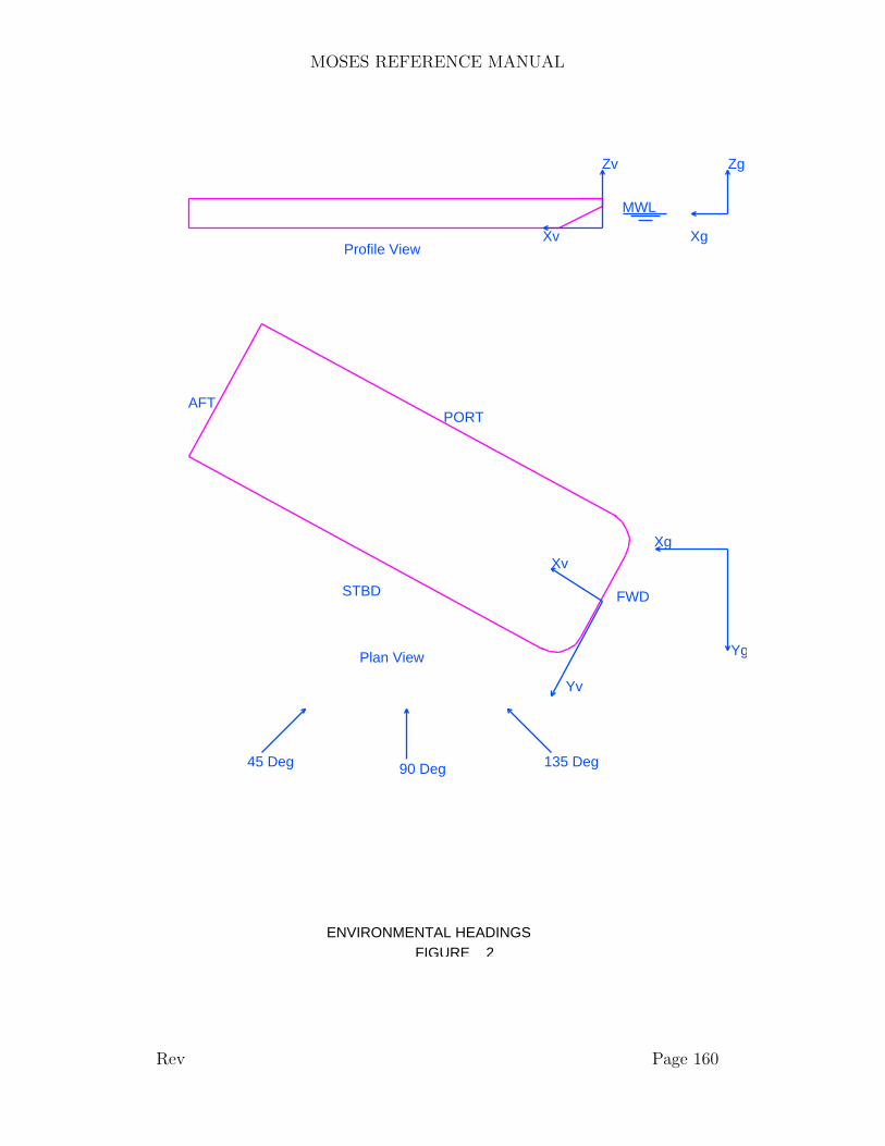
MOSES REFERENCE MANUAL
MWL
FIGURE 2ENVIRONMENTAL HEADINGS
Xv
Zv
Xg
Zg
Xv
Yv
Xg
Yg
FWD
AFTPORT
STBD
Plan View
Profile View
45 Deg 90 Deg 135 Deg
Rev Page 160

MOSES REFERENCE MANUAL
omitted, a value of 3.72 will be used. If DURATION is selected, the probablemaximum based on a specified duration will be reported. Here, one specifies theduration in seconds with PDATA.
To define the sea for a given environmental condition, one employs –SEA, –A SEA,–SPREAD, –SP TYPE, –SPREAD, –TIME, –MD PERIOD, –S PERIOD,–RAMP and –T REINFORCE options. In essence, the first two options definesthe basic sea condition and the others serve to instruct MOSES how to treat thedetails. In MOSES, one can have several different seas which will be added togetherto form the sea state to which the model will be subjected. –SEA is used to definethe first sea, and –A SEA is used to define subsequent ones. Other than this dis-tinction, the two options are identical. For either –SEA or –A SEA, SEA NAMEis the name of the sea. It must be either REGULAR, ISSC, JONSWAP, 2JON-SWAP or a name defined as a ”curve” with &DATA CURVE P SPECTRUM,&DATA CURVE F SPECTRUM commands, in the &DATA with GRID.Here, HS is the significant height (feet or meters), PERIOD is the period (sec.),SEA DIRECTION is the mean heading (deg.), and for a name of JONSWAP,GAMMA is the ”peakedness factor”. The precise definition of PERIOD dependsupon the value of TYPE specified with the –SP TYPE option or which was speci-fied on a &DEFAULT command. If TYPE is PEAK then period is the period atwhich the spectrum has a maximum. If it is MEAN, then the period at which thespectrum peaks is given by
Tp = 1.2958*PERIOD
Notice that for an ISSC spectrum (GAMMA = 1), PERIOD is the mean period. Forvalues of GAMMA other than one, PERIOD has no meaning other than that givenabove.
If one is using a sea defined by a wave grid, then the period and height are ignored,and for anything other than JONSWAP, GAMMA is ignored. When an inputspectra is used, the input values are scaled so that the sea will have the specifiedsignificant height. Also with an input spectrum, one can omit the PERIOD, and thespectrum will be as input. If one does add a period, the spectrum will be scaled sothat the peak frequency will move according to an ISSC spectrum.
All of the ISSC, JONSWAP and 2JONSWAP spectra can be represented by the
Rev Page 161
MOSES REFERENCE MANUAL
equation:
S(f) = alpha * 172.8 * HS**2 * z * exp [ –1948.184*z ] * p / f
where f is the frequency in rad/sec.,
z = 1. / ( f * Tp ) **4p = GAMMA ** exp [ ( beta – 1) **2 / ( 2 * sigma**2) ]beta = Tp * f / ( 2 * pi )
sigma is .07 for frequencies less than the peak and .09 for those greater than thepeak, and alpha is a parameter computed to make the total area under the spectrumequal to HS**2 / 16. With these spectra, the significant height is twice the squareroot of the area. For 2JONSWAP, the value of GAMMA is not input, instead,it is obtained from the DNV guidelines. Unfortunately, their relationship betweenGAMMA and the ”slope” is dimensional. What we have is
s = Tp * sqrt( g/(2*pi*Hs) )
GAMMA = 5 for s < 4.5GAMMA = 1 for s > 6.2GAMMA = exp( 5.86 – .94 s) for 4.5 <= s <= 6.2
There is almost never a need to define a spectrum by its ordinates. Many usersthink that because someone gives them a Bretschneider or a PM spectrum, thatthey need to resort to such measures, but this is not necessary. The problem comesfrom the lack of consistency in the manner in which sea data is provided. All of thesea spectra we know of have the same form as the one above. The difference is inthe manner in which the period variable is specified. Sometimes, a peak period isspecified, sometimes a significant, sometimes a mean, other times none at all. Theeasiest case is when one is given a PM or Pierson Moskowitz spectrum and no periodis specified. Here, one can use
PERIOD = sqrt ( ( 23.27 * 2 * pi * HS ) / g )
which says that the ratio of mean wave length to height is 23.27. In other cases,one should find where the specified spectrum has a peak and use the result above toobtain PERIOD.
The –SPREAD option controls the spreading of the seas, and EXP is the exponentwhich defines the wave spreading function, F:
F(THET) = COS(H – THET)**EXP for –pi/2 < THET < pi/2
Rev Page 162
MOSES REFERENCE MANUAL
F(THET) = 0 Otherwise
Here H is the mean wave heading. If the –SPREAD option is not used, a value of200 will be used for EXP. The –MD PERIOD option defines the periods, TD(I), atwhich wave drift forces will be generated when performing a time domain simulation.If they are omitted, the values specified via &DEFAULT will be used. Similarly,the –S PERIOD option defines a set of periods which will be used to synthesizewave frequency excitation. If they are omitted, the values specified via &DEFAULT–PERIOD will be used. In the case when a spectrum will be used to synthesizea time domain sample of a sea, the –RAMP, –TIME, and –T REINFORCEoptions are used to control the synthesis.
The variable RAMP TIME of the –RAMP option defines the time interval overwhich the sea will be linearly ramped from zero to its full value. If either option–RAMP or –T REINFORCE are omitted, the values defined via &DEFAULTwill be used.
The –TIME option sets the observation time and time increment of the synthesis.Here, TOBSERV, is the end time of the synthesis and DELTA TIME is the timeincrement. TTRA SET can be used to set a time translation. If TTRA SET is anumber, then this number translates time equal zero to this time. The simulationwill still begin at zero, but the environment at time equal zero will have the same asthat at the specified time. If TTRA SET and CYCLES are omitted, a translation ofzero will be used. If, however, TTRA SET is FIND then MOSES will attempt tofind a time so that during the synthesis a peak will be found which corresponds to theprobable maximum during a simulation with NCYCLES. In essence, the followingalgorithm is used:
• Compute the wave amplitudes,• If the amplitude is within 85 percent of the desired value, keep it as a viable
peak,• Keep finding peaks until there are 10 candidates.• Pick the candidate which is closest to the desired value.
It is possible that a ”good” solution to this problem will not be found. In particular,if NCYCLES is too large then no peak greater than that specified may be found. Theother extreme is if NCYCLES is too small in comparison to the observation time.Here, it may not be possible to get a time interval in which a peak will not be toolarge. The above scheme will, however, normally yield a result which is larger thanthat requested.
The option –T REINFORCE is used to pick the phases of the frequency compo-
Rev Page 163

MOSES REFERENCE MANUAL
nents. If the sea was defined as a regular wave, then the phase is zero. If, however,the sea was specified via a spectrum another method is used. Here, the phases arechosen as
phi(i) = –TB * w(i)
Here, phi(i) is the phase for the ith component, w(i) is the frequency (rad/sec) of theith component, and TB is a time. By using this scheme, you always get the samesea, and two time domain simulations will yield identical results. The time, TB, hasan interesting interpretation – it is a time at which all of the components reinforce,i.e. at this time the amplitude of the sea is the sum of all of the Fourier coefficients.Depending on the number of components you use, this sum is ”unreasonably” largeand this time is to be avoided during the simulation. Thus by default, it is set tobe a large number. If you need to change it to perform Monte Carlo simulations,use –T REINFORCE. Finally, if TB is negative, then the phases will be chosenrandomly using the absolute value of TB as the seed.
The wind is defined with the options –WIND, –W PROFILE, –W PERIOD, –W DESIGN –W SPECTRUM –W HISTORY, and –W MD CORRELATIONoptions. The –WIND option defines the wind speed, WIND SPEED, which is themean wind speed in knots, and WIND DIRECTION is the direction from which thewind blows. The –W PROFILE option defines how the wind will vary with height.Here, WP TYPE can be ABS, API, NPD or POWER. If TYPE is ABS, thenheight coefficients will be computed according to the ABS rules. If WP TYPE isAPI or NPD, the wind variation with height will be according to the specified code.If, however, WP TYPE is POWER, then EXP is the power which defines the powerlaw for wind variation. In other words, if EXP is equal 1/7, then the wind will varywith height according to a 1/7 power law. To specify the type and duration of thedesign wind speed, the –W DESIGN option is used. Here, DTYPE can be eitherAPI or NPD, and DURATION is the design wind speed average in seconds.
To define the temporal or frequency behavior of the wind, one uses either the –W SPECTRUM or –W HISTORY options. The first of these defines the type ofwind spectrum to be used. For this option, STYPE can be API, NPD, HARRIS,DAVENPORT OCHI, or the name of a spectrum previously defined with &DATACURVE with a TYPE of either F SPECTRUM or P SPECTRUM. Most ofthese standard spectra can be found in a paper ”Wind Turbulent Spectra for DesignConsideration Of Offshore Structures”, OTC 5736, by Ochi and Shin. The APIspectrum is taken directly from the API–RP2a 21st edition and the NPD spectrumis taken from NORSK STANDARD N–003, ”ACTIONS and ACTION EFFECTS”Rev1, February 1999. It should be noted that there is a contradiction between theturbulence factor and the wind spectrum for the NPD spectrum. For this case,
Rev Page 164

MOSES REFERENCE MANUAL
MOSES uses the spectrum for the shape and the intensity for the variance.
Instead of using a spectrum, the time variation of the wind can be defined with the, –W HISTORY option, This option instructs MOSES to use a previously definedwind history of HISTORY NAME. This history is defined with &DATA CURVEW HISTORY.
The –W PERIOD option defines the periods, TW(I), at which wind forces will begenerated when performing a time domain simulation. If they are omitted, the val-ues specified via &DEFAULT will be used. Finally, –W MD CORRELATIONdefines the relative phase of the wind velocity components with the wave drift com-ponents. If FACTOR is 0, then the two have phases 90 degrees apart, if FACTORis one, then the two phases are the same. Intermediate values of FACTOR producerelative phases between these two extremes.
The current is defined via the –CURRENT option. There are two styles for thisoption. With the first, one simply specifies a current speed, VC (ft/sec or m/sec),constant with depth and the direction from which it comes, CURRENT DIRECTION(deg.). The second method is used to define more complicated currents. Here,PRO NAME(i) is the name of a current profile defined in the &DATA CURVEC PROFILE and CURRENT DIRECTION is again the direction from which thecurrent comes. Notice that one can define several different profiles from differentdirections. MOSES will combine each of the profiles to yield the true current velocityat any depth.
The tide is defined by the –TIDE option where CHANGE is the change in (feet ormeters) of the water level. The water depth is set with the –DEPTH option, usingunits of feet or meters.
The marine growth on the structure is specified by the –M GROWTH option,where MG NAME is a name which has been defined via the &DATA CURVEM GROWTH command.
If one wishes to include internal pressure or temperature effects during a structuralanalysis, he must specify the internal pressure and temperature distribution. Thisis accomplished with the –T PRESSURE option with TMP NAME being a namewhich has been previously defined via the &DATA Menu with a T PRESSUREcommand.
When an environment is used for computing forces or stresses spectrally, one caneither combine the deviation with the mean, or omit the mean by using the –USE MEAN option depending upon whether or not YES/NO is YES or NO.
Rev Page 165
MOSES REFERENCE MANUAL
If this option is omitted, then the mean will be used.
As mentioned previously, some of the environmental data must be defined in a sepa-rate menu. This is accomplished by issuing
&DATA ENVIRONMENT
One can then define basic environmental data. At the conclusion of defining envi-ronmental data, one should then issue END &DATA to exit the menu.
The command
T PRESSURE, TMP NAME, OBJECT(1), TMP(1), INP(1), GH(1), SC(1), \OBJECT(2), TMP(2), INP(2), GH(2), SC(2), ..
defines a temperature and internal pressure distribution within the elements whichcan be referenced by the name TMP NAME. Here, OBJECT is the name of the objectto which the temperature TMP(i) (degrees F or degrees C) and internal pressuredistribution will be applied. The pressure distribution is defined by a given gagepressure (ksi or mpa), INP(i), measured at a global height GH(i) (feet or meters), andSC(i) is the specific gravity of any fluid contained inside the element. If OBJECT(i)is two node names (they may include wild characters, but must begin with a *),the attributes will apply to all beams between those two nodes. If OBJECT(i) is anattribute class name (begins with a ∼), then the attributes will apply to all elementswhich belong to classes which match OBJECT(i). If OBJECT(i) does not begin witheither an * or a ∼, then the attribute will be applied to all members whose namesmatch OBJECT(i).
The command
ENVIRONMENT, ENV NAME, –OPTIONS
stores a complete environment in the database. The options for this command arethe same as those for &ENV, described earlier.
The command
S GRID, GRID NAME, GRID TYPE, DEPTH, HEIGHT, PERIOD
is used to define a wave grid. Here, GRID TYPE is the type of wave used to gen-erate the grid and it must be either: REGULAR, STOKES, STREAM, or IN-PUT. For this command, GRID NAME is the name of the wave grid, and DEPTH,HEIGHT, and PERIOD are the water depth (feet or meters), wave height (feet or
Rev Page 166

MOSES REFERENCE MANUAL
meters), and period (sec.) used in generating the wave as shown in Figure 3. Ifone of the first three values is specified, MOSES will automatically generate a wavegrid using either a regular wave, a Stokes fifth order wave, or a wave generated by astream function algorithm. If INPUT is specified for GRID TYPE, then the user isplaced into another sub–menu where the grid can be defined. This is accomplishedvia the commands:
HORIZONTAL, X, WELEVVERTICAL, Z(1), VX(1), VZ(1), AX(1), AZ(1), ........END INPG
The HORIZONTAL command defines the locations along the wave where the grid isto be defined. X is the distance from the wave crest (feet or meters), and WELEV isthe elevation of the wave above mean water level (feet or meters). Once the horizontallocation has been defined, one should input as many VERT commands as necessaryto define the wave velocity and acceleration. Here, Z(i) is the depth of the pointbelow the mean water surface, negative for points above the mean water surface,VX(i) and VZ(i) are the horizontal and vertical wave velocities (ft/sec or m/sec),and AX(i) and AZ(i) are the horizontal and vertical wave accelerations (ft/sec**2 orm/sec**2). When the grid has been completely defined, one should issue END INPGto return to the ENVIRONMENT sub–menu.
There is a string function:
&ENV(INFO )
Which returns information about the current environment. Here INFO must beS HEIGHT, S PERIOD, S GAMMA, S CREST, S HEADING, S SP TYPE,S PERIOD, W SPEED, W DIRECTION, W SPECTRUM, W DESIGN,W PROFILE, W PERIOD, or C SPEED, C DIRECTION, WAT DEPT,TIDE, WATER, MD PERIOD. T OBSERVE, T INCREMENT, RAMP,T REINFORCE, The values beginning with S return information about the sea,the ones beginning with C return information about the surface current, the onesbeginning with T and RAMP return information about the time, the ones beginningwith W return information about the wind, and the ones beginning with S returninformation about the sea. WAT DEPT returns the water depth and WATERreturns the specific gravity of water.
Rev Page 167
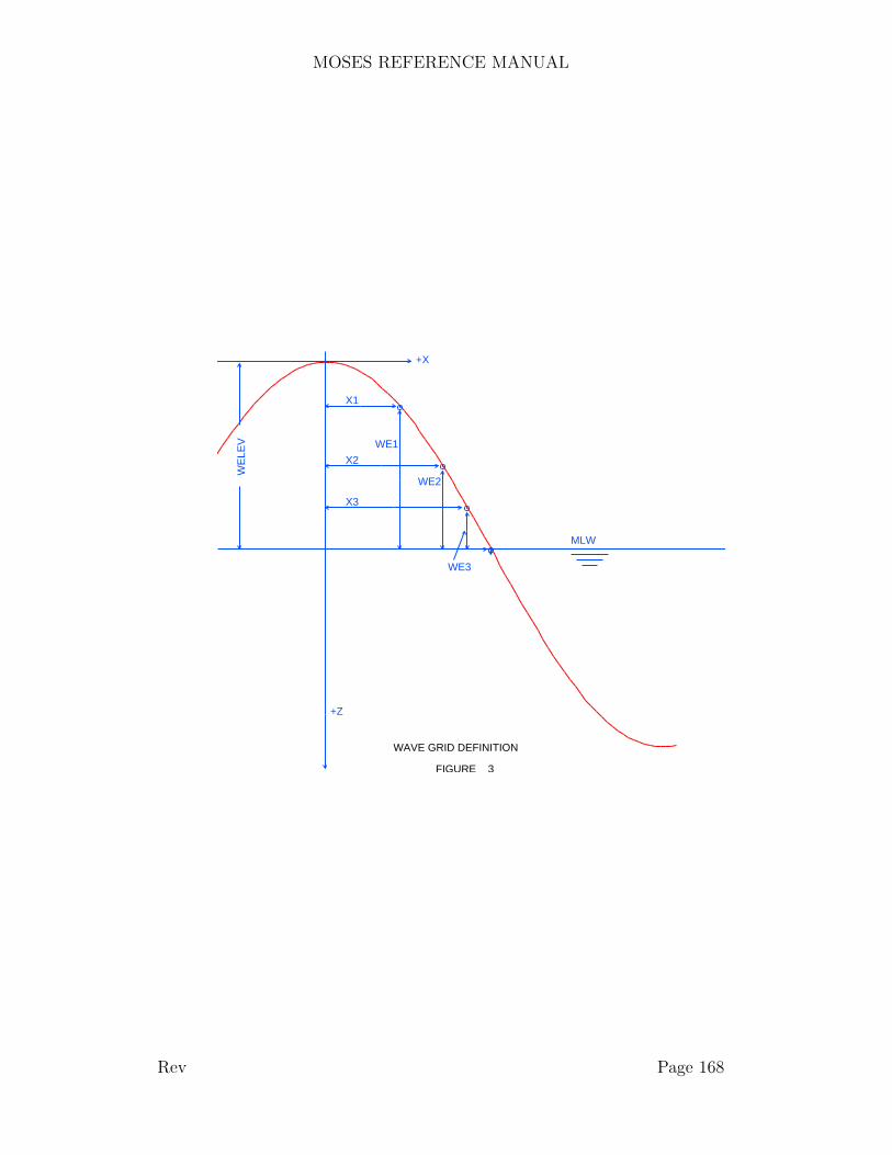
MOSES REFERENCE MANUAL
WAVE GRID DEFINITION
FIGURE 3
WE1
WE2
WE3
X1
X2
X3
MLW
WE
LEV
+X
+Z
Rev Page 168
MOSES REFERENCE MANUAL
XII.G.1 DurationsThe purpose of a DURATION is to associate a time of exposure to an environment.With mooring line fatigue this is done directly on the &ENV command itself. For allother cases it is done in the &DATA DURATION Menu. This is done in one oftwo ways depending on the type of analysis performed.
For either type of analysis, the following command is used.
STRPOST&DATA DURATION, DURATION NAME, PRC NAME, –OPTION
where the only available option is:
–TDOM, DUR TIME
Here DURATION NAME is the ”duration name”. When asking for fatigue resultsone selects the durations to be applied, and PRC NAME is the process name forwhich the duration will be applied. The –TDOM option signifies that one wishes toperform time domain fatigue on the process PRC NAME and that the total durationof this process is DUR TIME in days. This is all that is required for a time domainprocess.
When DURATION is used without the –TDOM option, a sub–menu is enteredwhere frequency domain fatigue data will be defined. In other words, for frequencydomain the DURATION command is followed by a series of records of the form:
WTIME(i), –OPTIONS
Where the available options are:
–SEA, SEA NAME, THET, HS, PERIOD, GAMMA–A SEA, SEA NAME, THET, HS, PERIOD, GAMMA
Here, WTIME(i) is the time (days) which the system will be exposed to the seastatedefined by the remainder of the record. Here the parameters SEA NAME, THET, HS,PERIOD, and GAMMA are the same as those used to define a sea with the &ENVcommand. If a duration environment is defined with more than one spectrum thenMOSES provides two ways to compute the ”average period”. The choice is governedwith the –T AVERAGE option of the &PARAMETER command.
When all of the duration has been defined, one exits the sub–menu with an
Rev Page 169

MOSES REFERENCE MANUAL
END DURATION
command. Notice that one can perform both time domain fatigue and frequencydomain fatigue in the same run, and both types of fatigue can be computed for thesame process.
Rev Page 170

MOSES REFERENCE MANUAL
XII.H Fatigue and Cycle Counting
Fatigue is a particularly complex topic, as there are several components to consider:
• The SN curve, which defines the number of cycles of a given maximum (hotspot) stress the material can withstand without breaking,• The Stress Concentration Factors (SCF) which define maximum stresses in
terms of the nominal ones, and• The duration which defines lifetime history of the environment to which the
structure has been exposed.
Normally the result of interest is a Cumulative Damage Ratio (CDR). This is simplya sum of ratio of the fraction of the life used for all stress ranges. Sometimes, however,one wishes to view the loading history independently of the SN curve. Thus, MOSEShas the capability for counting either load cycles or stress cycles sorted into bins. Onecan compute fatigue (or cycles) for BEAMs, PLATES, tubular JOINTs and mooringlines and the details will vary with type. In general, one can compute fatigue ineither the time or frequency domains.
One is really interested in fatigue at all points in an element, but in reality we onlyconsider it at a set of ”fatigue points”: the ends, at points along a beam wherethe section changes, or at welds. Generalized plates are special in that fatigue iscomputed at the centroid of each subelement.. To really complicate these matters,some fatigue points have automatic methods to compute stress concentration factorand others do not. In particular, MOSES has automated methods for computingstress concentration factors for: tubular connections, tube/cone connections, andtubular joints. Stress concentration factors must be manually associated with allother fatigue points.
In MOSES there are two ways to compute fatigue damage, on an element by elementbasis, or on a tubular joint basis. The reason for the two methods is that for tubularjoints, there is a body of knowledge for automatically computing the SCFs and theassociated hot spot stresses. For non tubular joints, the information is much lessextensive. Thus, for tubular members, one can do joint fatigue to capture the damageat the ends, but one must do element (beam or generalized plate) fatigue to get CDRsat intermediate locations. Also, element fatigue must be used to get the CDRs atthe ends elements which are not part of tubular joints.
As with stress concentration factors, an SN curve must be associated with each fatiguepoint. Again, tubular joints are special in that one normally has only two choices forSN for a tubular joint and the association of SN is different for doing JOINT fatigue
Rev Page 171
MOSES REFERENCE MANUAL
than it is for doing BEAM fatigue.
The definition of the environmental history depends on whether a time domain or afrequency domain simulation is being used. For frequency domain, a set of RAOs arecomputed and they are used along with a scatter diagram of environments which actfor a specified time. In the time domain, one time domain simulation is performedper process. Load cases are defined at a reasonable number of times during thissimulation and the system solved for the time traces of the stresses. A RainflowCounting technique as outlined in ASTM E–1049, ”Standard Practices for CycleCounting in Fatigue Analysis” is then used to compute the stress cycles and perhapsthe cumulative damage. These results are ”scaled” by the ratio of duration time tosimulation time. The results are summed over the selected durations, so one cancompute fatigue in both domains and over all lifetime situations.
If a duration environment is defined with more than one spectrum then MOSESprovides two ways to compute the ”average period”. The choice is governed with the–T AVERAGE option of the &PARAMETER command.
In the following we specifically discuss the role of the &REP SELECT command,but any of the options discussed for this command can be issued on the option whichrequests fatigue or cycle information. In other words:
&REP SELECT –SN XJOINT POST FATIGUE
produces the same result as
JOINT POST FATIGUE –SN X
The same can be said of the BEAM POST or PLATE POST commands.
Rev Page 172
MOSES REFERENCE MANUAL
XII.H.1 Defining SN CurvesBefore any fatigue can be computed, an SN curve must be defined. This is accom-plished with the command:
&REP SELECT –OPTIONS
and the available options are:
–SN, CURVE, TYPE, S(1), N(1), ..... S(n), N(n)–THICK SN, TO, POWER, MAXCOR, FLAG–S IMP FACTOR, SFACTOR–F STRESS, S MULT
Once a curve has been defined, one need only specify
–SN, CURVE
to select, CURVE, for use in computing cumulative damage ratios. MOSES has a setof curves automatically generated and hence these do not need to be defined to beused. The automatic ones are: the
• API X and API XP curves from API–RP2A 21st edition, the• API WJ, API WJG API WJP, API WJ WET, API WJG WET, API WJP WET,
API CJ, API CJG, and API CJP from API RP2A 2nd supplement to the21st edition, the• API CHAIN,and API WIRE curves from API–RP2F,• HSE TP curve from HSE, and the• DNV B1, DNV B2, DNV C, DNV C1, DNV C2, DNV D, DNV E,
DNV F, DNV F1, DNV F3, DNV G, DNV W1, DNV W2, DNV W3,DNV T, DNV B1 WET, DNV B2 WET, DNV C WET, DNV C1 WET,DNV C2 WET, DNV D WET, DNV E WET, DNV F WET, DNV F1 WET,DNV F3 WET, DNV G WET, DNV W1 WET, DNV W2 WET, DNV W3 WET,and DNV T WET curves from DNV RP–C203 (2008).
For the WJ and CJ curves, the ones with ” G” include weld improvement due togrinding and the ones with ” P” include improvement due to hammer peening.
To define a curve, one first specifies TYPE which defines the type of curve. TYPEshould be STRESS for a normal curve, or TENSION for a curve like the WIREand CHAIN curves. The values S(i) and N(i) define the stress (or tension / breaktension) and the corresponding number of cycles. After the curve is defined, one usesthe –THICK SN option to define a correction which depends on thickness. Mostdocuments say that this is a reduction of the SN curve, but in MOSES, it is viewed
Rev Page 173

MOSES REFERENCE MANUAL
as an increase in SCF. Thus, our factor is greater than one and is the inverse of whatwould be a reduction of SN. The only real difference is that POWER here is positivewhere with a reduction it is negative. Here, TO, is the nominal thickness (inches ormm) and POWER is the power of the correction; i.e. the curve will be corrected bya factor, FACT, where:
FACT = MIN ( (THICK/TO)**POWER, MAXCOR )
and THICK is the thickness. The details here are governed by FLAG. If FLAGis USE BRACE, then FACT computed as above with THICK equal to the bracethickness is used for both the brace and the chord. Otherwise FACT is computedfor both the brace and the chord using their respective thicknesses. Here, MAXCORcan be omitted and it will be set to ”infinity”.
The –S IMP FACTOR option is used to define a ”stress improvement factor”.This factor simply reduces the SN curve by SFACTOR; i.e. the stress in the SNcurve is divided by SFACTOR.
Neither the API X nor XP curves built into MOSES have any thickness correction!The reason is that there is quite a bit of ambiguity in API–RP2A about how to treatthis question. In particular, depending on the details, no correction may be needed.If you do need it, however, it can be included with:
&REP SELECT –SN X –THICK SN 1 .25 1.5 USE BRACE
This tells MOSES to use a correction on any brace having a thickness greater than 1inch with a power of .25 up to a maximum factor of 1.5 and to use the brace factorfor the chord. The 1.5 maximum comes from the fact that RP2A says that the Xcurve need not be reduced below the XP curve, and the X curve reduced by a factorof 1./1.5 has the same endurance limit as the XP curve.
The –F STRESS option is a simple way of overcoming a deficiency in most of thepublished SN curves; they are only defined over a limited range of cycles. Most ofthe time, this does not matter, but the algorithm MOSES uses strictly considers onlydamage which occurs in the specified range. Without any further action, a beam withhigh stress might actually accumulate less damage if the stress were increased! Thisoccurs because increasing the stress moves more of the harmful cycles outside therange of the SN curve. The value S MULT is a multiplier which MOSES multipliesby the RMS of the stress spectrum to check for this bad behavior. If the productS MULT * RHS is greater than the stress at the first point of the SN curve, thenthe stochastic integration is not performed, but damage is accumulated based on thefirst point in the SN curve. This is simply an estimate to keep one out of trouble.By default, S MULT is 3.72, but you can set it to 0 to strictly obey the standard
Rev Page 174

MOSES REFERENCE MANUAL
algorithm.
Rev Page 175

MOSES REFERENCE MANUAL
XII.H.2 Associating SN Curves with PointsAn SN curve must be associated with each fatigue point. The details differ basedon the type of fatigue being computed, but in all cases it is accomplished with an–SN option. For mooring line and tubular joint fatigue, the ”current” SN name willbe used; i.e. the last name specified on either a &REP SELECT command or itsequivalent.
For elements (other than mooring lines) there are three ways to define them: ona &DEFAULT command, on the ∼CLASS command, or on the element definitioncommand. In any case failure to include a definition results in the last definitionbeing used; i.e.
• The –SN specified on the element command is used,• If no –SN is specified on the element command, than specified on the class
definition is used,• If no –SN is specified on the class definition, then that defined on the &DE-
FAULT is used.
For the &DEFAULT command, the default SN curves at various points on an elementare defined with the option
–SN, TYPE(1), SN1 A, SN1 B, SN1 R, \TYPE(2), SN2 A, SN2 B, SN2 R, ......
Here, TYPE(i) defines a section type and must be either: TUBE, CONE, BOX,WBOX, PRI, IBEAM, G IBEAM, TEE, CHANNEL, ANGLE, D ANGLE,LLEG, or PLATE. SN1 A is the SN curve name for the A end of the element,SN1 B is for the B end, and SN1 R is for all remaining segments. This sequence canbe repeated for as many section types as desired. Also, if only one SN curve name isprovided, the same SN name is used for all locations along the element. If two SNnames are specified, the first name applies to the ”A” end of the element, and thesecond SN names applies to the ”B” end and all segments in between. Of course, theSN curve specified here must be defined to MOSES using the appropriate commands,such as &REP SELECT.
For the element and class definition commands, the situation is a bit different. Here,we know how many fatigue points we have so we can directly define an SN curve foreach one of them. Thus, for classes, we have the option for each segment of
–SN CURVEA, CURVEB
Here, CURVEA is the SN curve which will be used at the beginning of the segmentand CURVEB is the curve used at the end of the segment. If one uses two names for
Rev Page 176

MOSES REFERENCE MANUAL
each segment, the one in the middle will be defined twice. If this is done, the seconddefinition will actually be used; i.e. the first curve specified will, in fact, be used forthe beginning of the segment. Also, CURVEB needs to be specified only on the lastsegment.
For elements, we have
–SNi, CURVE
which defines the SN curve for the ”ith” fatigue point of the element to be ”CURVE”.Here, –SNA defines curve at the A end, –SNB defines curve at the B end, –SN1defines curve at the end of the first segment, etc.
Rev Page 177
MOSES REFERENCE MANUAL
XII.H.3 Associating SCFs with Tubular JointsLike SN curves a set of stress concentration factors (SCFs) must be associated witheach fatigue point. The details differ based on the type of fatigue being computed.For tubular joint fatigue, the SCFs will normally be computed based on the jointgeometry and the load path and is controlled by a set of options on the point definitionor ED POINT command, and the default for all of these parameters is specified onsimilar options of the &DEFAULT command. The applicable options are:
–CO SCF, SCF TYPE–LEN FACTOR, FRACHOL–MAX CHD LEN, MAXCHOL–CHD FIXITY, CHD FIX–SCF BOUNDS, MIN SCF, MAX SF
This computation is controlled by the –CO SCF option. The valid values forSCF TYPE are K&S, API, MARSHALL, and EFTHYMIOU. With the au-tomatic computation of SCFs, two values are computed: one for the root of theweld on the brace side, and one for the root of the weld on the chord side. The–LEN FACTOR, –MAX CHD LEN, and –CHD FIXITY options define pa-rameters which are used by some of the methods in computing the SCFs. For somemethods, the SCFs depend upon the length of the chord. FRACHOL is a fractionof the actual chord length which will be used. The default value of FRACHOL isone. MAXCHOL is the maximum length which will be used and its default value is”infinite”. Suppose that the chord length was 200. If FRACHOL is set to .5 andMAXCHOL is 50, the program will first set the length to be used to .5*200. It willthen take the maximum of 100 and 50 and use this value in the computation. The–CHD FIXITY, option defines the ”chord flexibility” CHD FIX. This is a measureof the bending support at the ends of the chord. It should be a number between.5 and 1. The first of these corresponds to the chord ends being pinned and thelater fixed. The –SCF BOUNDS option defines minimum and maximum valuesfor SCFs. Any computed SCF smaller than MIN SCF or greater than MAX SCFwill be replaced with the limit.
If stiffeners are associated with either of the two chord classes, then they will beused in computing the ”crushing” of the joint, in computing the code check for thejoint, and in computing the stress concentration factor for the joint. The numberof stiffeners will be the sum of the number for both chord segments. For situationswhere two classes define the chord with different stiffener attributes, then the prop-erties of the last one encountered will be used. Here, the stiffeners are ”smeared”over the effective length (or true brace footprint of the joint). The SCFs computedby whichever method are reduced according to ”Lloyd’s Register of Shipping Recom-
Rev Page 178

MOSES REFERENCE MANUAL
mended Parametric Stress Concentration Factors for Ring Stiffened Tubular Joints”.
Rev Page 179
MOSES REFERENCE MANUAL
XII.H.4 Associating SCFs with Element PointsIn computing fatigue in elements, the element SCFs are used. For elements thereare four ways to define them: on a &DEFAULT command, on the class definitioncommand, on the element definition command, or in some cases from the tubularjoint SCFs. In any case failure to include a definition results in the last definitionbeing used; i.e.
• For intermediate fatigue points between tubular sections, an SCF will be com-puted based on the algorithm specified on the –IN SCF option on the &PA-RAMETER command,• For intermediate fatigue points between tubular and conical sections, an SCF
will be computed as specified in API RP2A or DNV (they are the same).MOSES will also check for two tubes that have no braces and will computean inline SCF as if the change in section was internal to the beam itself. Forother cases, the –SCF specified on the element command is used, If no –SCF isspecified on the element command, then that specified on the class definitionis used, If no –SCF is specified on the class definition, then that defined on the&DEFAULT is used.• In the case where one of the ends of a tubular element is part of a tubular joint,
then a part of the joint SCF will be used for the SCF of the element at thatend.
To define the ”inline” SCF between two tubular sections, then the
–IN SCF, TYPE
option of &PARAMETER is used. There type must be either DNV or a number.The number is the exponent, e, used in computing the SCF according to:
SCF = 1 + A * B
A = 3 ( T2 – T1 )/ T1
B = T1**e / ( T1**e + T2**e)
Where T1 and T2 are the tubular thickness. If DNV is specified a value of 2.5 willbe used for e. Here T2 is greater than T1.
For the &DEFAULT command, the default SN curves at various points on and
Rev Page 180
MOSES REFERENCE MANUAL
element are defined with the option
–SCF, TYPE(1), SCF(1), ....
The –SCF option defines default stress concentration factors for different types ofsection. Here, TYPE(i) defines a section type and must be either: BOX, PRI, BU,W, M, S, HP, WT, MT, ST, L, C, MC, WBOX, DL, LLEG, or PLATE. Thevalues SCF(i) are the stress concentration factor for the corresponding type. Pleasenotice that one cannot define a default SCF for a tube. This would defeat the normalcomputation of SCF’s for joint fatigue. If you have a tube, want to do beam fatigue,and want an SCF other than 1, you need to manually do it on the command whichdefines the beam.
For class definition commands, we have the option:
–SCF SCF BEG, SCF END
Here, SCF BEG is the SCF which will be used at the beginning of the segment andSCF END is the curve used at the end of the segment. If one uses two SCFs foreach segment, the one in the middle will be defined twice. If this is done, the seconddefinition will actually be used; i.e. the first SCF specified will, in fact, be used forthe beginning of the segment. Also, SCF END needs to be specified only on the lastsegment.
The SCF definition for elements is accomplished with the –SCF option which isfollowed by from one to eight numbers. If there is no SCF option, then the defaultSCF defined for this class will be used. Here, –SCFA will change the values at thefirst end of the beam –SCFB will change them at the other end, and –SCF1 willchange them at the intersection between the first segment and the second, etc. If–SCF is used, then the stress concentration factor will be the same at all fatiguepoints. For the ends of the beam, the form of this option is:
–SCFi, VALUES(1), ... VALUES(n)
One can input 0, 1, 3, 4, 8, or 24 values. Zero values sets the SCFs to the defaultvalues. If 1 values is input, then it will be used as the SCF for axial and for strongand weak axis bending. If three values are input then they are the axial, strong axis,and weak axis binding SCFs.
The remaining numbers (4, 8, or 24) are used to override the computed SCFs whenthe beam is part of a tubular joint. The first four values here define the SCFs at thebrace at the saddle, crown, in plane bending and out of plane bending. If only fourvalues are given, then these will be repeated for all three load classifications and for
Rev Page 181

MOSES REFERENCE MANUAL
the chord. With eight values, the second four values define the SCFs for the chordand the brace/chord values will be used for all joint classifications. If twenty fourvalues are specified, the first twelve are for the chord in K joints, T&Y joints and Xjoints, and the last twelve are the corresponding values for the chord. K, T&Y, andX. (See section on Associating SCFs with Tubular Joints for more information).
Also, the ”joint SCFs” are used when computing beam fatigue. Here, the maximumof the crown and saddle SCFs and the maximum inplane and out of plane SCFs forall classifications will be used at the end when computing beam fatigue. This willresult in beam fatigue which will be a bit less that that computed at the same endby joint fatigue, but it is not excessively conservative for slamming fatigue.
Rev Page 182
MOSES REFERENCE MANUAL
XII.H.5 Beam Fatigue Due to SlammingIf one is computing fatigue in the time domain, then the damage due to slammingis correctly included. When fatigue is considered in the frequency domain, however,the situation is quite different. Here, an element which is out of the water in themean position occasionally enters the water and a slam event occurs. MOSES has aspecial algorithm to compute fatigue due to these slamming events.
This computation depends on the parameters specified on either the BEAM POSTcommand or the
&REP SELECT –OPTIONS
and the options applicable here are:
–SLA COEFFICIENT, S COE–SLA FIXITY, S FIXITY–SLA DAF, S DAF–SLA CDAMP, S CDAMP–SLA MULTIPLIER S VEL(1), S MUL(1), ... S VEL(n), S MUL(n)
The data will be discussed below, and only beams that are out of the water in themean position and of which are allowed to have forces due to added inertia will beconsidered for beam fatigue.
First, notice that here we do not have the normal frequency domain phenomenon.Instead, we have an occasional impulsive load which acts on the beam, and when theload is removed, then beam experiences a free vibration decay. Thus, according toDNV, the force per unit length on a beam due to slamming is:
W = .5 * rho * D * S COE * abs ( V * Vv )
Where rho is the water density, D is the tube diameter, and the option –SLA COEFFICIENTdefines S COE is the slam coefficient (nominally 3), and V is the relative velocity be-tween the beam and the water, and Vv is the relative velocity vertically. Now, themaximum bending moment in the beam, assuming that the load is uniformly appliedover the length, can be written as
M = S FIXITY * W * L * L
Here the –SLA FIXITY is used to define S FIXITY which is a number that dependson the fixity of the beam. It is 1/8 if the beam is simply supported and 1/12 if it is
Rev Page 183

MOSES REFERENCE MANUAL
built in. This, in turn gives a maximum stress in the beam of
s = S DAF * SCF * R * M / I
Where R is the beam radius, I is the section inertia, SCF is the stress concentrationfactor, and the option –SLA DAF defines S DAF is the dynamic amplification factorwhich is nominally 2.
After the impulse is applied and released, the beam will freely vibrate with decreasingamplitude
s(k) = s(k–1) * exp ( –200*pi/S CDAMP)
Here S CDAMP is the percentage of critical damping defined with the –SLA CDAMPoption. Now, the total damage due to a single impulse is
CDR = SUM [ 1./ N(s(k)) ]
Here, N is the number of allowable cycles at the stress s(k), and the sum continuesuntil there is no further damage.
There remain two unanswered questions: the first is how many slam events do wehave and what are the velocities associated with each slam event. The first questionis easily answered if one assumes that the slam events are Raleigh distributed. Inthis case, one simply computes the number of times in a given time that the probablemotion will exceed the mean. This gives us a slam velocity or number of slams perhour. The second question is not so clear. Suppose that we write the velocity as amultiple of the RMS.
V = f * Fmax * Vrms
Here V is the velocity which will be used, Fmax is the multiplier which gives the”maximum” event from the RMS, and f is a factor. If the slam velocity is ”low”then the slam events are associated with extreme events and the multiplier f shouldbe 1 so that the velocity used is the ”maximum” velocity. If on the other hand theslam velocity is high, then slams are not rare events and the multiplier should be oneappropriate to a normal event such as 1/Fmax. MOSES uses an linear interpolationfor f with the points in the table defined by the –SLA MULTIPLIER option. Thisoption defines a table of slam velocities, S VEL(k), vs. multipliers, S MUL(k). Bydefault, the table consists of three points: If the slams per hour are <= 1 then f is1, if the slams per hour are 10, then f = 1/1.86, and if they are >= 360, then f =1/3.72.
Rev Page 184
MOSES REFERENCE MANUAL
XII.I Forces
In MOSES, forces on the system are separated into nineteen named categories:
• WEIGHT: This is the weight of a portion of the system.• CONTENTS: The weight of ballast in compartments or fluid in an element.• BUOYANCY: The buoyancy of a portion of the system.• WIND: The wind force acting on a portion of the system,• V DRAG: The viscous drag acting on a portion of the system. This is the
velocity squared term in Morison’s equation, the viscous roll damping, or theviscous drag on a piece with the –CS CURRENT option. This can be eitheran excitation due to wave or current, or a damping in still water.• WAVE: This is the linear exciting force on a portion of the system.• R DRAG: The radiation damping due to hydrodynamics or that due to a
#DRAG load attribute.• SLAM: This is the force due to mass transfer into the system; i.e. it is the
velocity time the mass flow rate term in the equations of motion.• CORIOLIS: This is the force due to Coriolis acceleration. It also produces a
”slowly varying” force.• W DRIFT: This is the nonlinear part of the wave force, or the slowly varying
”wave drift force”. In MOSES, it does not contain an approximation of theCoriolis force. This is different than most other programs.• DEFORMATION: This is the force on a body due to deformation of the
body. This only occurs when a body has generalized degrees of freedom.• EXTRA: This is a ”extra” force that can be added to produce equilibrium in
a given configuration. This is useful to ”cover up” modeling errors or errors inthe environment.• APPLIED: This is a true force applied to a portion of the body.• INERTIA: This is the mass of the body times the acceleration.• A INERTIA: This is the added inertia times the acceleration.• C INERTIA: This is the inertia of the contents times the acceleration.• FLEX CONNECTORS: This is the force due to flexible connectors.• RIGID CONNECTORS: This is the force due to rigid connectors.• TOTAL: This is the sum of all of the other contributions.
The accuracy of the computation of forces on a plate or panel depends on the shapeof the panel. In particular, the results for more ”compact” panels is superior tothose which are ”long and skinny”. As a guide to the ”badness” of panels, a badnessmeasure is reported for the &SUMMARIES of panels and plates. Now, often this
Rev Page 185
MOSES REFERENCE MANUAL
measure is taken as the ”aspect ratio” of the panel; i.e.
R = W/H
Where W is the width, H is the height and W > H. This is all fine and good forrectangular plates, but when these enter the water the submerged portion is rarely arectangle.
To generalize this notion, in MOSES, we define badness as
B = P / [ 2 sqrt(pi*A) ] – 1.
Here P is the perimeter and A is the area. Notice that for a circle, B is zero and thatfor rectangular plates it increases with the increase of aspect ratio.
When added mass is computed for a panel or plate, the results from DNV–RP–C205are used. In particular, the force computations presented there for added mass forcesare tabulated as a function of B and interpolated based on the current values of Bfor the submerged portion of the plate.
Rev Page 186

MOSES REFERENCE MANUAL
XII.J Categories and Load Types
As mentioned above, the basic idea behind MOSES is that one defines attributeswhich the program then uses to compute loads. Now, an attribute may create loadfrom different sources. To distinguish these classes of loads, MOSES employs theconcept of the ”load type”, which is simply a name given to each of the sources ofloads, and is either: #DEAD, #WIND, #BUOY, #AMASS, or #DRAG, forthe intrinsic loads, or a user supplied name which begins with a # for the appliedloads. These names are used to control which type of load is applied to each loadattractor. Here, #DEAD is the load due to weight, #WIND to wind, #BUOY ishydrostatic pressure, #AMASS is hydrodynamic pressure, and #DRAG is viscouswater force.
For structural elements, one can select which of these forces will be applied. This isaccomplished with two options on either &DEFAULT, BEAM, or PLATE com-mands:
–USE, USE(1), USE(2), ..., USE(i)–NUSE, NOT USE(1), NOT USE(2), ..., NOT USE(i)
Here, the values of USE(i) and NOT USE(i) are the selectors for the names of theload types defined above. For example,
–USE @ –NUSE #WIND
Instructs MOSES to consider all of the load types except wind when computing theforce on an element. When a structural element is defined, MOSES first sets theload type flags to those defined with &DEFAULT. Then either of these optionsencountered on the definition itself serve to alter the settings defined by those from&DEFAULT.
The options defined above allow one to effectively define which elements are exposedto different environments. To give the user even more control, there is an additionalconcept, the Category. Each load attribute in MOSES has a category name associatedwith it and each category name has a set of multipliers for each load type. Thecategory name is associated with a load attribute when it is defined in a mannersimilar to the load type flags. The &DEFAULT command accepts two options:
–BAS CAT, BASE CAT NAME–EXT CAT, EXTRA CAT NAME
the –BAS CAT option defines a Category name, BASE CAT NAME, to the load at-tributes defined with the structural elements themselves. –EXT CAT defines a Cat-
Rev Page 187
MOSES REFERENCE MANUAL
egory name, EXTRA CAT NAME, for any additional load attributes (those whichbelong to Load Groups or those defined with a #ELAT command). Now, when aelement or load attribute is defined, the default Category (either BASE CAT NAMEor EXTRA CAT NAME) will be associated with it. This default association can bechanged with the option
–CATEGORY, CAT NAME
which associates CAT NAME with the attribute. This option is available on BEAM,or PLATE commands and any command which begins with a #. Reports areavailable which produce sums of weight and buoyancy by Category. As an example,consider
BEAM BODY NAME –CATEGORY INSIDE –NOTE Interior Beams ∼CLASS..
This defines a beam, associates it with a Category, INSIDE, and defines a descriptionof the Category ”Interior Beams”.
Load Groups have a multiplier for the total force of the group. Initially this multiplieris set to one.
Control of all of these multipliers is available with the command:
&APPLY, –OPTIONS
where the available options are:
–PERCENT–FRACTION–FORCE :NAME(1), VAL(1), .... :NAME(n), VAL(n)–LOAD GROUP :NAME(1), VAL(1), .... :NAME(n), VAL(n)–TIME NAME, C NAME–CATEGORY :CAT(1), :NAME(1), VAL(1), .... :NAME(n), VAL(n)–MARGIN :CAT(1), VAL INC(1), .... :CAT(n), VAL INC(n)
The first two options define the way the VAL(i) are interpreted. If a VAL is precededby a –PERCENT option, it is interpreted as a percent. If it is preceded by a –FRACTION, it is a multiplier. If neither of these options precedes a value, it isinterpreted as a percent. In essence, percents are divided by 100 to convert them intomultipliers.
The –FORCE option defines multipliers for user defined load sets. Here, :NAME(i)
Rev Page 188
MOSES REFERENCE MANUAL
are selectors for these sets and VAL(i) are the multipliers one wishes to associatewith the set. By default, all user defined load sets have a multiplier of zero. Thus,they will not be applied unless one uses this option.
The –LOAD GROUP option defines multipliers for load groups. By default, thesemultipliers are one. Thus, one normally does not need this option. One can, however,turn off the force due to a load group using this option. For example,
&APPLY –PERCENT –LOAD GROUP A NAME 50 –FRACTION B NAME0.50
will apply 50 percent of load group A NAME, and one half of load group B NAME.
The –TIME option define multipliers which vary with time. Here, NAME is thename of either a LOAD GROUP or a user defined load set and C NAME is thename of a curve which has been previously defined with a &DATA CURVE TIMEcommand. At each event during a time domain simulation, MOSES will interpolate amultiplier from the specified curve. If NAME is later specified with –LOAD GROUPor –FORCE options, the time variation will be ”turned off”.
The last two options control the load type multipliers for Categories. The –CATEGORYoption allows one to control the multipliers for all load types while the –MARGINoption sets only the #DEAD, or weight, multiplier. Here, VAL(i) are the same as forthe load group and load set options, while VAL INC(i) are increases; i.e. the multi-plier is really 100 or 1 plus VAL INC depending upon –PERCENT or –FRACTIONoption in effect. Here, :CAT(i) is a selector for the Categories for which multiplierswill be set and :NAME(i) are selectors for the load types. For example:
&APPLY –PERCENT –CATEGORY STR MODEL @ 0 #DEAD 105
will set the multipliers for category STR MODEL to all zero except for the weightwhich will be applied with a multiplier of 1.05.
There are three actions of the &INFO string function that can be used to obtaininformation about categories:
&INFO( ACTION, :SELCAT )
Here ACTION must be either WT CATEGORY, BU CATEGORY, or MU CATEGORYwhich will return the weights. buoyancies, or multipliers for the categories selectedby :SELCAT. For the first two, five tokens will be returned for each selected cate-gory: the name of the category, either its weight or buoyancy, and either its CG orCB. These are for either the current part or the last part selected with the –PART
Rev Page 189

MOSES REFERENCE MANUAL
option of a &REL SEL command. The CG or CB will be in the part system. TheMU CATEGORY action returns the name of the category and the category multiplierfor each selected category.
Rev Page 190
MOSES REFERENCE MANUAL
XII.K Bodies and Parts
The basic ingredients for performing a simulation are bodies. For simulation purposes,bodies are considered rigid, and composed of parts. A part is the smallest entity uponwhich a structural analysis can be performed. Bodies are connected by parts whichcontain special elements called connectors. In essence, a part is simply a namedportion of the model.
All properties of the system are described by the attributes of the parts. In otherwords, every attribute of the system must be an attribute of some part of the system.Thus, everything except bodies belong to some part.
In MOSES, each body, and each part will have a separate coordinate system associ-ated with it. Since MOSES can consider bodies which move in space, we also employa global coordinate system. The global system is fixed in time, and is used to locatepositions in space. Its origin is arbitrarily located on the water surface, and its Zaxis points upward.
The part coordinate system is used to define the geometry of a part. In other words,
• The location of the points,• The load attributes applied to the part, and• The resulting structural displacements of the elements.
Thus, the part system is used in defining the model and in the definition of thestructural deflections.
The body system is used for simulations. In most cases, the body system will beidentical to the part system of the part which has the same name as the body. Theaxes of the body system are parallel to the global system when roll, yaw, and pitchare zero. The orientation of the body system defines the orientation of the body bythree Euler angles, yaw, followed by a pitch, followed by a roll. An illustration of theglobal and part coordinate system along with a jacket and vessel body system duringa launch is shown in Figure 4.
To distinguish between different bodies and parts, a block concept is used; i.e., allof the data for a part and body is defined contiguously in the input. One definesthe different parts and bodies by &DESCRIBE commands. All of the data whichfollows one of these commands will be associated with this body or part until another&DESCRIBE command is encountered. This command also allows the user to alterthe attributes of the body as the analysis proceeds. The format of this command is:
Rev Page 191

MOSES REFERENCE MANUAL
RELATIONSHIP OF GLOBAL, BODY, ANDPART COORDINATE SYSTEMS - ALL Y-AXES OUT OF PLANE
FIGURE 4
XgXv
ZvZg
Zj
Xj Xp
Zp
j = jacket body systemv = vessel body systemp = part system for jacketg = global system
(z=0 at MWL)
&DESCRIBE BODY, BODY NAME, –OPTIONS
where the available options are:
–IGNORE, DOF(1), DOF(2), .....–GEN DOF, MODE SEL(1), MODE SEL(2), ....–S DAMPING, CFRACTION–SECTION, EI, X(1), SM(1), ....., X(n), SM(n)–LOCATION, X(1), X(2), ......–DMARK, DM NAME, *DPT(1), *DPT(2)–D DMARK, :DM NAME(1), :DM NAME(2), ......–PR NAME, PR NAME–MD NAME, MD NAME–MD FORCE, MD FORCE, MD RADIATION, MD CORIOLIS–MD PHASE, MD PHASE–FM MORISON, FM FACTOR–SPE MULTIPLIER, SPEMUL–SP ORIENT, VX, VY, VZ, HX, HY, HZ–SP HEIGHT, X, Y, Z–DT CONVOLUTION, DT CONV–FACT CONVOLUTION, CONV FACTOR–PERI USE, PER–WAVE RUNUP, YES/NO
To ease the difficulty of defining a model, whenever a body is defined, a part with thesame name is automatically defined. Any attribute defined before a part is specifically
Rev Page 192

MOSES REFERENCE MANUAL
defined becomes the property of the ”body” part. NOTICE that since everythingmust belong to some part of some body, a &DESCRIBE BODY should be at thebeginning of each set of data.
Normally, all bodies have six degrees of freedom. Sometimes, one wants to ”ignore”some of these degrees of freedom. This is accomplished with the –IGNORE option.Here, DOF(i) is the name of the degree of freedom to be ignored, and must be chosenfrom the list X, Y, Z, RX, RY, and RZ. When a degree of freedom is ignored, theforce in this degree of freedom is set to zero, and the inertia is set to a very largenumber.
Normally, bodies have six degrees of freedom. The option –GEN DOF, however,allows one to use previously computed vibration modes as generalized degrees of free-dom for a body. For a discussion on computing modes for a body, see the sectionon Extracting Modes. Here, MODE SEL(i) are selectors for the mode numbers onewishes to use. MODE SEL(i) can be a single number which selects that mode num-ber, or a pair of numbers A:B which selects all modes from A to B. Once a body hasmore that 6 degrees of freedom, some measure of its deformation and the deforma-tion inertia is accounted for in any equilibrium, time domain, or frequency domainanalysis. Thus, this is an excellent way to study the effect of flexibility on the results.To the user, however, the number of degrees of freedom make no difference in howto accomplish various tasks. The only effect is the computer resources required. The–S DAMPING option defines the modal damping which will be used for the gen-eralized degrees of freedom. Here, CFRACTION is the fraction of critical dampingto be used. If this option is omitted, .01 will be used.
Two options of &DESCRIBE BODY serve to override defaults when computinglongitudinal strength. The –SECTION option is used to define the ”section prop-erties”. Here, EI is the stiffness of the body. The X(i)s are the X locations along thebody where one wishes to compute longitudinal strength results, and SM(i) is thebody section modulus at X(i). If only a single location is specified, then MOSES willredefine this data so that results are computed at each station, and the section mod-ulus will be constant along the length of the body. For SM the units will be eitherft**3 or meters**3, and for EI, force–ft**2 or force–meters**2. If one simply wants todefine the locations at which the results are reported, he can use the –LOCATIONcommand.
The option –DMARK is used to define draft marks and –D DMARK is used todelete draft marks. Draft marks are rays along which one measures draft. Eachmark is defined by two points. The first point is the ”origin” of the draft markand the second is used to define the direction of the mark. Draft is the distancealong this ray from the first point to where the waterplane intersects the line. Here,DM NAME is a name given to the draft mark, *DPT(1) a point defining the origin of
Rev Page 193
MOSES REFERENCE MANUAL
the mark, and *DPT(2) is a point defining the direction of the mark. On should use a–DMARK option for each draft mark defined. When deleting marks, :DM NAME(i)are selectors which select the marks to delete.
The next two options: –PR NAME and –MD NAME, allow one to change thepressure packet name and the drift packet name associated with the body. Here,PR NAME and MD NAME are the new pressure or mean drift names. In mostcases, the mean drift database is created as a consequence of creating the pressuredatabase, and a discussion of the mean forces can be found in the section of theHYDRODYNAMICS MENU and in the subsection on mean drift.
The next three options allow one to change the multipliers used with the meandrift force. The –MD FORCE option defines three scale factors, MD FORCE,MD RADIATION, and MD CORIOLIS which are used in computing the total meandrift force. The last two of these are multipliers of the radiation and Coriolis con-tributions to the mean force as they are added to the diffraction contribution. TheMD FORCE factor multiplies the total mean force before it is accumulated. Thecurrent response operators for the current process are used when computing the ra-diation and Coriolis contributions. Finally, the –MD PHASE defines a phase angle(deg.) of the wave drift force in the frequency domain. Here, each drift force compo-nent will have a phase, PHASE, relative to the wave crest being at the origin. Thedefault for these options is set with &DEFAULT.
The next two options of &DESCRIBE BODY deal with viscous damping, and bothof them override defaults set with &DEFAULT. The –FM MORISON optiondefines a factor which will be multiplied by the computed viscous force to yield anapplied viscous force in the frequency domain. The option –SPE MULTIPLIERdefines the spectral linearization multiplier. When nonlinear quantities are linearizedwith a spectral linearization in the frequency domain, the RMS of the velocity ismultiplied by the factor SPEMUL and used in computing a constant drag coefficient.
When performing a simulation in the Static Process Menu, one needs to define twovectors which are used to measure the ”roll and pitch” angles and a point which isused to measure height. This is accomplished with the two options –SP ORIENTand –SP HEIGHT. All of these quantities used with these options are defined inthe part system of the body. The height used to terminate a lift is defined by X,Y, and Z. The pitch angle is defined as angle formed by the vector VX, VY, andVZ with the waterplane, and the roll angle is the angle formed by the vector HX,HY, and HZ with the waterplane. Here, VX, VY, and VZ are the components of avector in the part system which will be vertical when the jacket is in the installedcondition. If these options are omitted, the values defined with the same name on an
Rev Page 194
MOSES REFERENCE MANUAL
&DEFAULT command will be used.
The last four options provide the user ways in which to ”tweak” the hydrodynamicdata to suit his purposes. All these options use as defaults values defined with anoption of the same name on an &DEFAULT command. The first three optionscontrol the way the frequency dependent nature of the added mass and damping areconsidered in the time domain. As described in the Hydrodynamics section, mathe-matically, this results in a convolution. This convolution is, however, often difficultto deal with numerically. One of the leading causes of numerical instability is a badlybehaved convolution. In fact, with a convolution, it is possible to take too smalla time step! There is a limit to how much velocity history can be stored. For ex-tremely small time steps, this history may not be long enough to adequately describethe damping. The –DT CONVOLUTION option defines the time increment atwhich the convolution will be integrated. This must be equal or greater than the timestep at which the time domain is computed. If you use TIME STEP for DT CONV,then the convolution will be computed at the time steps used to integrate the equa-tions of motion otherwise it will be computed for times steps of DT CONV. Thisoption allows one to use a reasonable time step (around 1/4 second) to compute theconvolution and a smaller one to integrate the equations of motion which amelioratethe above problem. An alternative way of dealing with this problem is by using thelast two options. The –FACT CONVOLUTION option scales the kernel of theconvolution by CONV FACTOR before it is applied. If CONV FACTOR is zero,the convolution will not be added, and if CONV FACTOR is one, all of the convolu-tion will be added. The –PERI USE option allows one to replace the convolutionterms in the equations of motion with single added mass and damping matrices.The matrices used will be the frequency domain matrices at the specified period,PER. This eliminates any numerical problems with the convolution. The defaultshere CONV FACTOR = 1 and PER = 0, i.e. use all of the convolution in the timedomain.
In the time domain, the buoyancy is computed ”correctly” at each time step. Sincethe frequency domain forces already include the effects of the wave elevation, thisbuoyancy is computed assuming that the water surface is flat. If –WAVE RUNUPis used with a YES/NO of YES, then a different algorithm is used. Here, the watersurface is assumed to be adequately described by the incident potential and the”correct” Froude–Krylov force computed. When this option is used, the Froude–Krylov force is not included in the frequency domain forces applied.
The string function which returns data for bodies is:
&BODY(ACTION, BODY NAME, –OPTION)
Here, BODY NAME is the name of the body for which data is desired and ACTION
Rev Page 195

MOSES REFERENCE MANUAL
must be either: CURRENT, E NODES, P NAME, EXTREMES, DRAFT,LOCATION, VELOCITY, MXSUBMERGENCE, BOTCLEARANCE, NWT DOWN,MIN NWT DOWN, WT DOWN, MIN WT DOWN, E PIECES, I PIECES,MAX BUOYANCY, MAX CB, DISPLACE, CB, GM, G ROLL, I VECTOR,F WEIGHT, F CONTENTS, F BUOYANCY F WIND, F V DRAG, F WAVE,F SLAM, F R DRAG, F CORIOLIS, F W DRIFT, F DEFORMATION,F EXTRA, F APPLIED, F INERTIA, F AINERTIA, F CINERTIA, F FLEX CONNECTORS,F RIGID CONNECTORS, F TOTAL B CG, B WEIGHT, B RADII, B MATRIX,A CG, A WEIGHT, A RADII, A MATRIX, D CG, D WEIGHT, D RADII,or D MATRIX. The action CURRENT is special in that it should have no otherinput; i.e. no BODY NAME and no –OPTIONS. It returns the name of currentbody. All other action need a body name. If this name is omitted, the current bodywill be used. Thus if your model contains only a single body the name may be safelyomitted.
The action E NODES returns the names of the extreme nodes for the body, andP NAMES returns the names of the parts in the body. The action EXTREMESreturns the length, width, and height of a body where these quantities are mea-sured along the body X, Y, and Z axes respectively. The action DRAFT, thereading of the draft marks will be reported, while the actions LOCATION, VE-LOCITY, MXSUBMERGENCE, and BOTCLEAR, return the requested dataon the location of the body. WT DOWN and NWT DOWN will return a listof the down–flooding points of the specified type , and MIN WT DOWN andMIN NWT DOWN return the minimum height of the points about the water.
The actions E PIECES and I PIECES return a list of the external or internalpieces in the body. The actions MAX BUOYANCY and MAX CB return thenon–compartment buoyancy and its center when the body is completely submerged,while the actions actions DISPLACE, CB and GM return the current value ofthese things. For the actions CB, MAX CB, LOCATION, and VELOCITYthe option –GLOBAL can be used to change the returned data from being in thebody system to being in the global system. The G ROLL returns an angle whichis the angle of inclination of the body from the vertical. More precisely, if v is avertical vector represented in the body system, then G ROLL is the arc tangent ofthe sqrt(v(1)*v(1) + v(2)*v(2)) / v(3). The I VECTOR returns a vector which,if a moment is applied in this direction, will cause the inclination to increase, orI VECTOR = [ v(1), v(2), 0 ]/sqrt(v(1)*v(1)+v(2)*v(2)).
The actions which begin with a F return forces acting on the body. The datafollowing the specifies the type of load which will be returned. The meaning ofthese forces can be found in the section on FORCES.
If no option is specified, then the results are in the body system. Alternately, one
Rev Page 196

MOSES REFERENCE MANUAL
can specify –GLOBAL to return the values in the global system.
The remainder of the actions deal with the weight of the body. Those beginning witha B are applicable to the ”basic” weight of the body, those beginning with an A tothe ”apparent” weight of the body (basic weight plus weight of contents), while thosebeginning with a D deal with the ”define” weight for the body. What follows thedefine the type of data returned: WEIGHT for the weight, CG for the centroid of theweight, radii of gyration for RADII, and MATRIX for the 6X6 weight matrix (massmatrix divided by g).
Parts are defined similarly to bodies. In particular, the command to describe a partis:
&DESCRIBE PART, PART NAME, PART TYPE, –OPTIONS
and the available options are:
–MOVE, NX, NY, NZ, NRX, NRY, NRZ
or
–MOVE, NX, NY, NZ, *PT(1), *PT(2), *PT(3), *PT(4)
Here, PART NAME is the name to be given to the part, and PART TYPE is thepart type. The values one can use for PART TYPE are somewhat arbitrary, butthe two types of JACKET and PCONNECT have special significance. The parttype, JACKET, is used to denote the portion of the system which will be treateddifferently when the special transportation facilities of MOSES are employed. Toavoid confusion, elements which connect parts (elements which are connected tonodes in different parts) must belong to a part with a type of PCONNECT. Thus,the only elements which can span parts are connectors or PCONNECTors. APCONNECT part should not have any nodes which belong to it. There is a specialpart, GROUND, which does not belong to any body, and it is in this part thatelements which connect bodies reside. These elements which are called connectorsare quite important, since they define both the boundary conditions for a stressanalysis, and the constraints on the bodies for a simulation.
In most cases, the body system of a body will be coincident with the part system ofall parts belonging to the body. When certain types of connections (launch legs) aredefined, however, the body system will be altered as described later. Also, the usercan alter a part system using the –MOVE option. Here, NX, NY, and NZ are thelocation (feet or meters) of the origin of the part system with respect to the reference,and NRX, NRY, and NRZ are a set of Euler angles which defines the new orientation
Rev Page 197

MOSES REFERENCE MANUAL
of the part system. Alternately, if the second form of the command is used, the fourpoints define the orientation of the part system. Here, the part X axis will be fromthe midpoint of the segment connecting *PT(4) and *PT(2) to the midpoint of thesegment connecting *PT(3) and *PT(1). The part Z axis is defined by the crossproduct of the X axis with the vector from *PT(4) to *PT(2), and the Y axis is givenby the right hand rule. This option can be used both in defining a model, and whenediting one, but one can move a ”body part” (a part with the same name as a body)only while editing. Moving a body part is equivalent to changing the orientationof all of the parts of the body. When one is moving a part, the above data definesthe part system with respect to the ”body part” system and when moving a ”bodypart”, it defines the body part with respect to the body system. To orient the partsystem, suppose that the part and the reference systems are aligned, and that thepart system is rotated an amount NRZ about the reference Z axis. Next, rotate thepart system about the current part Y axis, and amount NRY, and finally rotate anamount NRX about the new part X axis.
The string function:
&PART(ACTION, PART NAME, –OPTION)
returns the current data about a part. Here, PART NAME is the name of the partfor which data is desired and ACTION must be either: CURRENT, MAX CB,MAX BUOYANCY, CG, WEIGHT, RADII, or E NODES. The action CUR-RENT returns the name of current part, while the WEIGHT, CG, and RADIIactions simply return the current weight, CG, and radii of gyration of the part.These are the ”dry” values of the part, without any compartment contents. TheMAX BUOYANCY and MAX CB return the non–compartment buoyancy itscenter when the part is totally submerged. If no option is specified, then the resultsare in the part system. Alternately, one can specify –BODY or –GLOBAL toreturn the values in another system. The action E NODES returns the names ofthe extreme nodes for the part.
After a set of bodies have been defined, it is necessary to place them in space as thepoint of departure for a simulation. This is accomplished via the command:
&INSTATE, –OPTIONS
where the options are:
–LOCATE, NAME, X, Y, Z, RX, RY, RZ–MOVE, NAME, DX, DY, DZ, DRX, DRY, DRZ–CONDITION, NAME, DRAFT, ROLL, TRIM
Rev Page 198
MOSES REFERENCE MANUAL
–POINT, *PNT(1), H(1), *PNT(2), H(2), .... *PNT(n), H(n)–DRAFT, DMARK(1), D(1), DMARK(2), D(2), .... DMARK(n), D(n)–GUESS, *NODE(1), *NODE(2), *NODE(3)–VELOCITY, NAME, VX, VY, VZ, VRX, VRY, VRZ–SL SET–LINES, :ACTIVE, :LSEL(1), TEN(1), :LSEL(2), TEN(2), ......–EVENT, EVE NUM–PREVIOUS–C FORCE, FLAG
The uses of the option keywords are: –LOCATE positions a body in space abso-lutely; X, Y, and Z are the global coordinates of a point on the body, and RX, RY,and RZ are the new Euler angles. The –MOVE option moves a body relative to itslast known position; in this case, the parameters are changes in position and orien-tation. –CONDITION is the same as –LOCATE except that only 3 degrees offreedom are necessary. Here, NAME is the name of either a body or a report point.If a point name is specified, then the position specified will be for that point. If abody is specified, then the location will be the location of the origin of the body.All of the units for these options are feet or meters and degrees. The three options–POINT, –DRAFT, and –GUESS all set the body according to the positions ofa set of points. With the –GUESS option, MOSES will change the orientation ofthe body so that the three nodes *NODE(1), *NODE(2), and *NODE(3) will lie inthe waterplane. Here, the three nodes cannot be colinear, and one cannot rotate abody ninety degrees. With –DRAFT, one specifies a set of draft marks and thedraft readings at the marks and with –POINTS, one specifies a set of points andthe height of these points above the water. MOSES then finds the draft, trim, andheel of the body that gives a ”best fit” to the data specified. The –VELOCITYoption defines the initial velocities of a body. Here again, the velocities specified arefor a point, a node, or the origin of the body in ft/sec or m/sec and degrees/second.
In general, when rigid constraints have been defined between two bodies, it is neces-sary to locate only one of the bodies. If one attempts to specify both, he may have adifficult time in locating the various bodies without violating a constraint. In otherwords, if only one body is specified, MOSES will locate this body and locate theother bodies in such a way as to satisfy the constraints. Also, one may not give abody a yaw (RZ) after you have connected launchways to it.
Positioning a system of bodies with connections is not a trivial task. The next twooptions are designed to minimize this difficulty. With these options, not only is theconfiguration of the system altered, but the lengths of some of the connectors arealso changed. The objective is to have the system be in equilibrium. The –SL SEToption simply computes the proper length for the tip–hook element of each tip–hook
Rev Page 199
MOSES REFERENCE MANUAL
set so that the lines have no slack in the specified configuration. This will probablynot be an equilibrium configuration, but it will be a good starting place for one.
The –LINES option instructs MOSES to alter the lengths of the flexible connectorswhich match :ACTIVE so the system will be as close to equilibrium as possible.The additional data controls the operation of the algorithm so that the connectorswhich match :LSEL(i) are altered to make the resulting tension (compression) in theconnector ”as close as possible” to that specified by TENS(i). For connectors whichare not selected by any of the selectors, the algorithm will attempt to make thetension as close as possible to the current tension. As mentioned above, the objectiveis an equilibrium configuration, but this cannot always be achieved. In particular,”anchor lines” cannot be used to alter the vertical force on a body, so that if one hasonly anchor lines, then there is no guarantee that the vertical forces will balance atthe conclusion of the command. Likewise, if one has only ”vertical” connectors, thehorizontal forces may be out of balance.
The –EVENT option sets the initial configuration to be the one at event EVE NUMof the current process, and –PREVIOUS is used to replace the initial state withthe ”previous” one. Here, ”previous” is the state existing before the last commandwhich changed the state before –EVENT was issued.
Finally, the –C FORCE option computes an ”extra” force on each body whichmakes the specified configuration an equilibrium configuration. This action occurs ifFLAG is COMPUTE. If FLAG is NO, the extra force will be set to zero.
In addition to the weights which were defined for elements and load groups, MOSESemploys an additional weight which can be applied to any part. This is called a”defined” weight and is controlled with the command:
&WEIGHT, –OPTIONS
where the available options are:
–COMPUTE, BODY NAME, ZCG, KX, KY, KZ–DEFINE, PART NAME, WEIGHT, XCG, YCG, ZCG, KX, KY, KZ–TOTAL, PART NAME, WEIGHT, XCG, YCG, ZCG, KX, KY, KZ
The first of these options is restricted to bodies while the others can be used withparts. For the first option, all data given should be in the body coordinate systemof the body, BODY NAME. For the others, all data should be in the part systemof the part PART NAME. The –COMPUTE option instructs MOSES to computethe weight so that, in the initial condition, the gravitational force will be equal to thesum of the other forces. The local Z center of gravity of the computed weight will
Rev Page 200

MOSES REFERENCE MANUAL
be placed at the specified location (ZCG). Alternately, a –DEFINE option defines aload with the weight and center of gravity specified. The option –TOTAL creates anadditional weight so that the total weight, center, and radii of gyration of the part willbe that specified. In either case, the weight which is defined will have radii of gyrationKX, KY, and KZ with respect to the point of application. Here the location of the cgand the magnitude of the radii of gyration are to be interpreted in the Body System.If bending moments are computed, the load will be represented as a trapezoidal loadacting over the entire body length. By default the loads resulting from the definedweight will be distributed to all nodes in the body part of BODY NAME or the partPART NAME.
As was implied above, while bodies are the basic ingredients of simulations, theyhave virtually no properties other than the parts which belong to them, and all ofthe physical properties of the bodies are inherited from their parts. This is quiteimportant since one can move parts between bodies, create new bodies, etc. Whileit may seem to be of limited use, this is not really the case. Suppose that one wishesto investigate the behavior of a jacket throughout its installation. First, one maywish to examine the loadout where the only thing of interest is the jacket itself.Here, a single body of ”jacket” is needed. Next, however, one wants to consider thetransportation. Here, a new body composed of the two parts: jacket and the bargewould be of interest. Finally, during launch, two bodies, the jacket and barge wouldbe used. The activity of bodies and parts is controlled with the command:
&DESCRIBE ACTIVITY, –OPTION1, –OPTION2 :SEL(1), :SEL(2), ..
and the available options are –BODY, –PART, –ACTIVE, and –INACTIVE.Here, one first uses either –BODY or –PART to specify what type of entity willbe changed. Next, he specifies either –ACTIVE or –INACTIVE to specify theactivity status. Any body (or part) selected after the second option will have itsactivity status set according to the option. As many options as one wants can beused on a single command. When a body is set inactive, its parts are not set inactive.There is no reason for this since only active bodies will be considered and this wouldmake it more difficult to reactivate a body.
In addition to the above, the entire system can be redefined with the command:
&DESCRIBE SYSTEM, –BODY, BODY NAME(1), PART(1), ..., PART(i),\
–BODY, BODY NAME(2), PART(1), ..., PART(i)
When this command is issued, all bodies and parts are set to inactive. Then thebodies named (BODY NAME(1), ....) are either activated or defined, and the partsspecified after the BODY NAME(i) and before the next –BODY are activated and
Rev Page 201

MOSES REFERENCE MANUAL
associated with the body BODY NAME(i).
Rev Page 202

MOSES REFERENCE MANUAL
XII.L Geometry
The geometry of the model is defined by a set of points in the part system. Thenames of all points begin with a *. The location of the points can be specified withrespect to either the part origin, or another point. At least one point in the model,however, must be specified with respect to the part system. Every point belongs toa part, and to allow for specifying fixed positions in space, there is a part which doesnot belong to any body, GROUND. Therefore, to define fixed locations in space onecan specify that the following points will be fixed by issuing &DESCRIBE PARTGROUND before the fixed points are defined. The part system of GROUND isthe global system.
Points to which one attaches structure have a special name, nodes. Each point whichis not a node will have a node associated with it. Any load associated with a pointis ultimately applied to the structure at the associated node. The associated node isthe node closest to the point which is in the ”associated node set.” Normally, this setwill be the set of all nodes. In some situations, however, one wishes to exclude certainnodes for being ”associated” and thus from attracting loads. This is accomplishedwith the command:
&DESCRIBE NODE NAS, PART NAME(1), :PNT SEL(1), ...
where PART NAME(i) is a part name, and :PNT SEL(i) is a selection criteria whichdefines the nodes which will not be associated.
Points which have both a chord, a single tubular member with the same outsidediameter and at least one other tubular element are called tubular joints. Tubularjoints are not true parts of a model since they inherit the most of their properties fromthe elements which intersect to form the joint. The concept of a joint is really onlyused in checking the codes which are applicable to joints and in computing fatigueat the intersection of the elements forming the joint.
Once a point has been defined, its properties can be changed with the ED POINTcommand, which is available either during an INMODEL or in the MEDIT menu.Its form is:
ED POINT, :PSEL, –OPTIONS
Here, :PSEL is a selector (selection criteria, or name which may contain wild charac-ters) of the points for which the options are applicable, and the options can be anyoption valid for the point definition command.
Often, it is desirable to obtain information about certain points on the bodies during
Rev Page 203

MOSES REFERENCE MANUAL
a simulation. The points at which these reports will be issued are defined by thecommand
&DESCRIBE INTEREST –OPTIONS
and the available options are:
–DELETE, :PNT SEL(1) .... :PNT SEL(i)–ASSOCIATE, :PNT SEL(1) .... :PNT SEL(i)
Here :PNT SEL(k) are selectors for points. The option –DELETE deletes the inter-est points selected by all of the selectors and –ASSOCIATE makes interest pointsof all points selected by the selectors. Interest points have a bit more informationassociated with them than the other types of points. In particular, each time the&DESCRIBE INTEREST, is issued, the global location of the interest point issaved. These locations are used for a reference in measuring ”motion” in severalreports.
Once a set of points for a part have been defined, they can be exported to a file forlater use with the command:
&EXPORT POINTS
Rev Page 204

MOSES REFERENCE MANUAL
XII.L.1 Defining PointsTo define a point, one issues the command:
*NAM, X, Y, Z, –OPTIONS
and the available options are:
–REFERENCE, *RPA, *RPB, ..–RECT–CYLINDER–SPHERICAL–LOCATION, XO, YO, ZO, RX, RY, RZ–LOCATION, XO, YO, ZO, *PT(1), *PT(2), *PT(3), *PT(4)–DEL, DOF(1), .... DOF(i)–JNTCLASS, PRCK, PRCT, PRCX–BBC MUL, MULT–EFF CHD LEN, ECHD LEN–CO SCF, SCF TYPE–LEN FACTOR, FRACHOL–MAX CHD LEN, MAXCHOL–CHD FIXITY, CHD FIX–MIN SCF, MIN SCF
where *NAM is the name of the point defined, and X, Y, Z are the coordinates (feetor meters) in the ”current point system” defined by the &DEFAULT command. Ifthe option –REFERENCE is employed, then the coordinates are relative to thespecified points; otherwise, they are with respect to the part origin.
If one reference point is specified, then X, Y, and Z define a vector from this referencepoint to point *NNAM. If two points are specified, then X specifies the distance fromthe point *RPA to point *NNAM, along a line from *RPA to *RPB, and Y and Zare ignored. If three points are specified, then they will define a local coordinatesystem with the origin being at the first point, the x axis being from point 1 to point2, the z axis being perpendicular to the plane formed by the three points, and the yaxis given by the right hand rule. Again, X, Y, and Z are local coordinates in thissystem. If four points are specified, then a point is first located at the intersection ofthe two lines which connect *RPA and *RPB, and *RPC and *RPD. The X, Y, andZ coordinates then define the vector from this point to point *NNAM. Rememberthat if one changes the coordinates of a point being referenced, then the coordinatesof the defined point will also change. Some examples of using reference points are
Rev Page 205

MOSES REFERENCE MANUAL
shown below:
*PT3 10 –REFERENCE *PT1 *PT2
This will create a point 10 feet (or meters) from *PT1 along a line formed by *PT1and *PT2. This example is handy for defining points along a battered jacket leg.
*PT5 –REFERENCE *PT1 *PT2 *PT3 *PT4
This will create a point at the intersection of the lines formed by points *PT1 and*PT2, and *PT3 and PT4, which is useful for defining points at the middle of Xbraces.
If one wished to temporarily override the current system, he may do so by specifyingany of the options –RECT, –CYLINDER, –SPHERICAL, or –LOCATIONwhich were discussed with the &DEFAULT command.
The option –DEL is used to delete the degrees of freedom of a point which specifiedby DOF(i) which must be either X, Y, Z, RX, RY, or RZ. If no DOFs are specified,then all degrees of freedom will be fixed. Notice that this option only has meaning ifthe point is also a node.
All of the remaining options define the ”joint” behavior of points. MOSES auto-matically classes joints based on the load path. In some rare cases, one may wishto override the automatic joint classification. This can be accomplished with the–JNTCLASS option. Here, PRCK, PRCT, and PRCX are the percentages of K,T, and X joint types used to classify a joint. When this option is used, the specifiedclassification for all load cases.
In Joint Crushing MOSES treats the joint as a two dimensional ring. Two basicassumptions here are that the braces do not alter the stresses in the ring and thatan effective length of the chord is used to distribute the load. The –BBC MULoption allows a factor of the bending stress under a brace to be used. In other words,if one believes that the brace will prevent any bending stress in the chord underits footprint, then he should specify a value for 0 with the –BBC MUL option.The opposite, conservative, view is that the brace has no effect in the bending of thechord where one specifies a value of 1 for MULT. Of course, one can specify any valuebetween these two. The –EFF CHD LEN option is used to change the effectivechord length for Joint Crushing from the default behavior computed according toAPI RP2A for both joints with and without rings.
The remainder of the options control the computation of SCFs for tubular joints.
Rev Page 206

MOSES REFERENCE MANUAL
These options were discussed in the section Associating SCFs with Tubular Joints.
Rev Page 207

MOSES REFERENCE MANUAL
XII.L.2 Geometry String FunctionsThe string function for points is one of the most useful, and its form is:
&POINT(ACTION, DATA, –OPTION)
Here, ACTION must be either COORDINATES, D NODE, PART, EULER ANGLES,N 2NODES, N BOX, RATIO, DEFLECTION, HOOK LOC, OFFSET, CLOSE,NEAREST, or REL MOTION. The details of DATA vary with ACTION, but nor-mally DATA will be one or more point names. If ACTION is COORDINATES,this function returns the location of the point specified with DATA. Here, the lo-cation returned will be in the part system, unless one of the options –BODY or–GLOBAL has been specified. If the point has not been defined, a null string willbe returned. One can use this function during an INMODEL, to define locationswhich may be required, provided that the point referenced has been previously de-fined. If ACTION is D NODE, the function will return the distance between thetwo points specified via DATA. If ACTION is PART, the part name of the pointspecified with DATA is returned.
When changing frames of reference, the ACTION EULER ANGLES may be useful.This action returns a set of Euler angles from three points specified via DATA. Theseangles will establish the new x axis along the line from first point to second, a new Zaxis perpendicular to the plane formed by the three points, and a new Y axis givenby the right–hand rule. The Z axis is defined by the cross product of the X axis andthe vector from the first to the third point.
The ACTION N 2NODES returns all points along the line segment between thefirst point specified via DATA and the second one. These points will be in order withthe first point specified being the first point returned and the second one specified asthe last one returned.
The remaining values ACTION are different than those above in that the DATAare not strictly point names. The ACTION N BOX is different from the others inthat the data here is a set of global coordinates: X1, X2, Y1, Y2, Z1, and Z2. Thefunction will return all points which are in the ”box” defined by the six planes definedby these coordinates. The ACTION RATIO will return the last value of joint unityratio computed for the specified point, and an ACTION of DEFLECTION willreturn the three components of the last computed deflection of the point.
The ACTION HOOK LOC has a form for DATA of: *NN1, LEN1, *NN2, LEN2,....., *NN4, LEN4, and is used to find the global position of a hook which is connectedto points *NN1, *NN2, etc. It assumes that the harness lengths are LEN1, LEN2, ...respectively. This function is useful primarily in setting up a lifting problem when
Rev Page 208

MOSES REFERENCE MANUAL
one models the sling as a collection of flexible connectors.
The values of ACTION OFFSET and CLOSE are used to find offsets. Normally,they are used in the definition of connectors. The form of DATA for OFFSET is:*POINT, :SEL, X, Y, Z and for CLOSE PART NAME, :SEL, X, Y, Z. Here, X,Y, and Z are locations (feet or meters). For both values of ACTION, MOSES findsthe point closest to a specified location but they differ in detail. For an ACTIONof OFFSET, the specified point is the location of *POINT plus the X, Y, and Zspecified, and any point which matches :SEL in a part different than that of *POINTis a candidate. The string returned is –GO1, the x, y and z values of the offset fromspecified point to the ”close” point, and the string *POINT itself. For CLOSE, thespecified point is simply the location in the part PART NAME defined by X, Y, andZ, and all points which match :SEL are considered for being ”close”. In either case,the vector returned is represented in the part system of the ”close” point. As anexample, consider:
CONNECTOR ∼CC &POINT(OFFSET *1 @ 0 0 10)
This will define a connector of class ∼CC. End 1 of the connector is at a physicallocation of *1 plus 0 0 10 in the part system of *1 and end two is at *1. Thisconnection is actually defined via the closest point and an offset and the commandset to MOSES will look like
CONNECTOR ∼CC –GO1 XX YY ZZ *B22 *1
where XX, YY, ZZ, and *B22 will be values computed so that the end of the connectoris at the correct location.
The ACTION of NEAREST takes a point name and a selector and returns thepoint which matches the selector closest to the given point. In particular:
&POINT(NEAREST *R *R@)
will return the name of the point which begins with *R (and which is not *R itself)that is closest the point *R.
Another useful ACTION is REL MOTION. Here, data is two point names *P1,*P2, and six numbers: X–, X+, Y–, Y+, Z–, and Z+. What the function returns isthe minimum and maxima of the relative location between the two points and thevalues input, i.e. the output is part of the input which has been modified. This isbest seen by example. Suppose that one issues:
&SET ENVEL =
Rev Page 209

MOSES REFERENCE MANUAL
&SET ENVEL = &POINT(REL MOT *1 *2 %ENVEL )
You will find that at this point X– = X+, Y– = Y+, and Z– = Z+, and X–, Y–, Z–is the vector from *1 to *2 in the *1 body system. If you issue the second of thesecommands several times, the result will be that ENVEL will contain the extremesof the relative position between the two points. From the above example, if thisACTION is used with null data, the accumulation is initialized. Also, the valuesreturned are in feet or meters.
Often, one wants to transform vectors from body to global coordinates and conversely.This is easily accomplished with the string function:
&V TRANSF(ACTION, BODY NAME, DATA)
Here, ACTION must be either V B2G, V G2B, V P2B, V B2P, L B2G, L G2B,L P2B, L B2P, F B2G, F G2B, F P2B, or F B2P and DATA is either three orsix coordinates (feet or meters) or six force components (bforce, bforce–feet or me-ters). The function takes the input and transforms it, returning the same numberof components as DATA input. If ACTION begins with: a V then a simple vectorrotation will be performed, with an L a rotation and a translation will be performed,and with an F a force transformation will be performed. The remainder of ACTIONdefines the direction of the transformation. The action B2G transforms a body rep-resentation into a global one, and G2B the inverse. The action P2B transforms apart representation into a body one, and B2P the inverse.
Rev Page 210
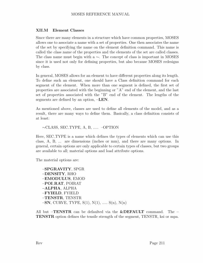
MOSES REFERENCE MANUAL
XII.M Element Classes
Since there are many elements in a structure which have common properties, MOSESallows one to associate a name with a set of properties. One then associates the nameof the set by specifying the name on the element definition command. This name iscalled the class name of the properties and the elements of the set are called classes.The class name must begin with a ∼. The concept of class is important in MOSESsince it is used not only for defining properties, but also because MOSES redesignsby class.
In general, MOSES allows for an element to have different properties along its length.To define such an element, one should have a Class definition command for eachsegment of the element. When more than one segment is defined, the first set ofproperties are associated with the beginning or ”A” end of the element, and the lastset of properties associated with the ”B” end of the element. The lengths of thesegments are defined by an option, –LEN.
As mentioned above, classes are used to define all elements of the model, and as aresult, there are many ways to define them. Basically, a class definition consists ofat least:
∼CLASS, SEC TYPE, A, B, ..... –OPTION
Here, SEC TYPE is a name which defines the types of elements which can use thisclass, A, B, ... are dimensions (inches or mm), and there are many options. Ingeneral, certain options are only applicable to certain types of classes, but two groupsare available to all; material options and load attribute options.
The material options are:
–SPGRAVITY, SPGR–DENSITY, RHO–EMODULUS, EMOD–POI RAT, POIRAT–ALPHA, ALPHA–FYIELD, FYIELD–TENSTR, TENSTR–SN, CURVE, TYPE, S(1), N(1), ..... S(n), N(n)
All but –TENSTR can be defaulted via the &DEFAULT command. The –TENSTR option defines the tensile strength of the segment, TENSTR, ksi or mpa.
Rev Page 211

MOSES REFERENCE MANUAL
The default value of TENSTR is 1.66 times the yield stress.
MOSES uses the class properties to compute various loads which will act on the body.The options:
–WTPLEN, WTPFT–DISPLEN, DPFT–BUOYDIAMETER, B DIAMETER–DRAGDIAMETER, D DIAMETER–WINDDIAMETER, WOD–AMASDIAMETER, AMOD
can be used to alter the properties which will be used to compute the loads. Nor-mally, the weight per length is computed from the true cross–sectional area and thedensity. If, however, the –WTPLEN option is specified, the weight per unit lengthwill become WTPFT (bforce/blength). The buoyancy for an element is computedas the sum of that arising from a diameter and a displacement per unit length.For tubular members, the displacement per length is zero and the diameter is theOD. For non–tubular elements, the diameter is zero and the displacement per unitlength is the element cross–sectional area times the density of water. One may al-ter this with the –DISPLEN and –BUOYDIAMETER options. Here, DPFTis the new displacement per unit length (bforce/blength) and B DIAMETER is the”buoyancy diameter” (inches or mm). The wind force, viscous drag, and addedmass are all computed based on an equivalent diameter (inches or mm). These canbe altered via the options: –DRAGDIAMETER, –WINDDIAMETER, and–AMASDIAMETER.
Once a class has been defined, it can be redefined with the command:
ED CLASS, ∼CLASS NAME, SEGNO, ......
Here, ∼CLASS NAME and SEGNO define the class and the segment which are beingedited, and the remainder of the command is the same as the class command. Theonly thing that the segment will inherit from the previous definition is the lengthor percent length. If SEGNO is omitted, the first segment will be redefined, and ifSEGNO is greater than the last segment defined, the last segment will be modified.For example,
ED CLASS ∼CLASS NAME 1 TUBE 60 1.5 –FY 42
will change the diameter, thickness and yield strength of the first segment of the class
Rev Page 212

MOSES REFERENCE MANUAL
∼CLASS NAME to the values specified.
To add a segment, specify a value of zero for SEGNO. The ED CLASS commandworks in the input channel through INMODEL, or under the MEDIT menu.
A string function is available that provides information regarding classes, and hasthe following form:
&CLASS(INFO, CLS NAM, SEGNO)
where INFO must be either ELEMENTS, N SEGMENT, TYPE, DIMEN-SION, FRICTION, DENSITY, EMODULUS, SPGRAVI, ALPHA, FYIELD,POI RATIO, TENSTRENGTH, B TENSION, WTPLEN, DISPLEN, BUOY-DIAMETER, DRAGDIAMETER, WINDDIAMETER, AMASDIAMETER,SECTION, PERLENG, LENGTH, REFINE, RDES, POINTS, REFER-ENCE, T STIFF, L STIFF, CFB, F TYPE, R SPACE, P FY, M P, ETA,P N, SCF, SN, PLATE DI, NAME DIM, NAME SEG, CLUMP, SOIL,PYMULT, TZMULT, QWMULT, SEND, SLOPE, DEPANC, IG STIF, PR M THRUST,PR EFFICIENCY, PR T ALIMITS, PR R ALIMITS, RR ALPAH, PR GAMMA,or PR R DIST. Here CLS NAM is the name of the class used to return informa-tion, and SEGNO is the segment number of the class. Most of these return values ofthat one sets with options of the same name on a class command. Some, however,require more information. When INFO is TYPE, the string function returns thetype of class, such as H CAT, B CAT, ROD, SL ELEM, GSPR for flexible classes,or any of the various structural section types, such as PLATE or TUBE. A value ofN SEGMENT returns the number of segments in a class, while a value of ELE-MENTS provides the element names using the specified class name. When INFOis DIMENSION, the dimensions of the specified segment of the class are returned.These dimensions could be diameter for class types such as H CAT, or cross sectiondimensions for structural classes. The value of INFO of NAME DIM returns toname of the dimensions returned with DIMENSION, e.g. Diameter and Thickness.Finally, the value of INFO of NAME SEG returns the name of the segment type,e.g. Rod.
Rev Page 213
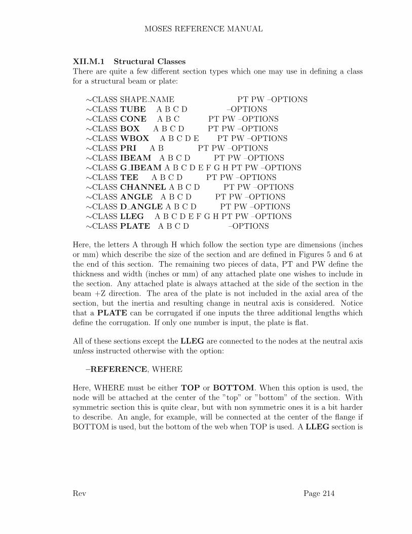
MOSES REFERENCE MANUAL
XII.M.1 Structural ClassesThere are quite a few different section types which one may use in defining a classfor a structural beam or plate:
∼CLASS SHAPE NAME PT PW –OPTIONS∼CLASS TUBE A B C D –OPTIONS∼CLASS CONE A B C PT PW –OPTIONS∼CLASS BOX A B C D PT PW –OPTIONS∼CLASS WBOX A B C D E PT PW –OPTIONS∼CLASS PRI A B PT PW –OPTIONS∼CLASS IBEAM A B C D PT PW –OPTIONS∼CLASS G IBEAM A B C D E F G H PT PW –OPTIONS∼CLASS TEE A B C D PT PW –OPTIONS∼CLASS CHANNEL A B C D PT PW –OPTIONS∼CLASS ANGLE A B C D PT PW –OPTIONS∼CLASS D ANGLE A B C D PT PW –OPTIONS∼CLASS LLEG A B C D E F G H PT PW –OPTIONS∼CLASS PLATE A B C D –OPTIONS
Here, the letters A through H which follow the section type are dimensions (inchesor mm) which describe the size of the section and are defined in Figures 5 and 6 atthe end of this section. The remaining two pieces of data, PT and PW define thethickness and width (inches or mm) of any attached plate one wishes to include inthe section. Any attached plate is always attached at the side of the section in thebeam +Z direction. The area of the plate is not included in the axial area of thesection, but the inertia and resulting change in neutral axis is considered. Noticethat a PLATE can be corrugated if one inputs the three additional lengths whichdefine the corrugation. If only one number is input, the plate is flat.
All of these sections except the LLEG are connected to the nodes at the neutral axisunless instructed otherwise with the option:
–REFERENCE, WHERE
Here, WHERE must be either TOP or BOTTOM. When this option is used, thenode will be attached at the center of the ”top” or ”bottom” of the section. Withsymmetric section this is quite clear, but with non symmetric ones it is a bit harderto describe. An angle, for example, will be connected at the center of the flange ifBOTTOM is used, but the bottom of the web when TOP is used. A LLEG section is
Rev Page 214
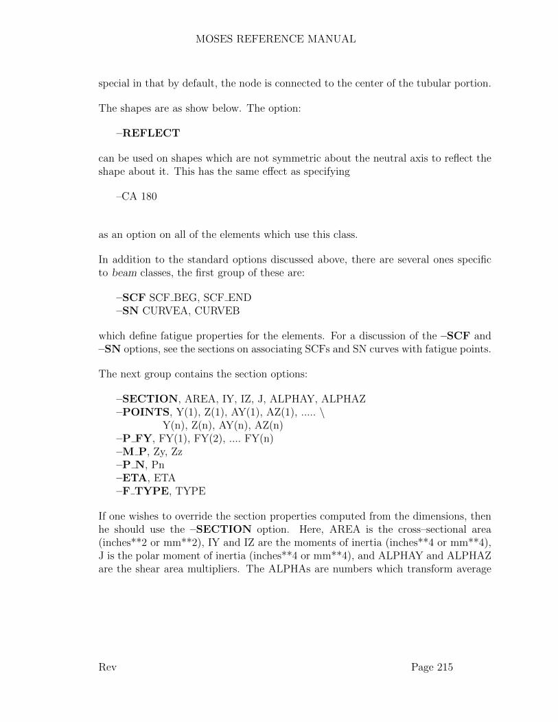
MOSES REFERENCE MANUAL
special in that by default, the node is connected to the center of the tubular portion.
The shapes are as show below. The option:
–REFLECT
can be used on shapes which are not symmetric about the neutral axis to reflect theshape about it. This has the same effect as specifying
–CA 180
as an option on all of the elements which use this class.
In addition to the standard options discussed above, there are several ones specificto beam classes, the first group of these are:
–SCF SCF BEG, SCF END–SN CURVEA, CURVEB
which define fatigue properties for the elements. For a discussion of the –SCF and–SN options, see the sections on associating SCFs and SN curves with fatigue points.
The next group contains the section options:
–SECTION, AREA, IY, IZ, J, ALPHAY, ALPHAZ–POINTS, Y(1), Z(1), AY(1), AZ(1), ..... \
Y(n), Z(n), AY(n), AZ(n)–P FY, FY(1), FY(2), .... FY(n)–M P, Zy, Zz–P N, Pn–ETA, ETA–F TYPE, TYPE
If one wishes to override the section properties computed from the dimensions, thenhe should use the –SECTION option. Here, AREA is the cross–sectional area(inches**2 or mm**2), IY and IZ are the moments of inertia (inches**4 or mm**4),J is the polar moment of inertia (inches**4 or mm**4), and ALPHAY and ALPHAZare the shear area multipliers. The ALPHAs are numbers which transform average
Rev Page 215

MOSES REFERENCE MANUAL
Y
Z
CATALOG OF SECTIONSFIGURE 5
TEE
TW
A
BC
D
ANGLE
TW
A
BC
D
CHANNEL
TW
A
BC
D
PRI
TW
A
B
G_IBEAM
TW
A
BF
G
C
D
E
H
IBEAM
TW
A
BC
D
Rev Page 216
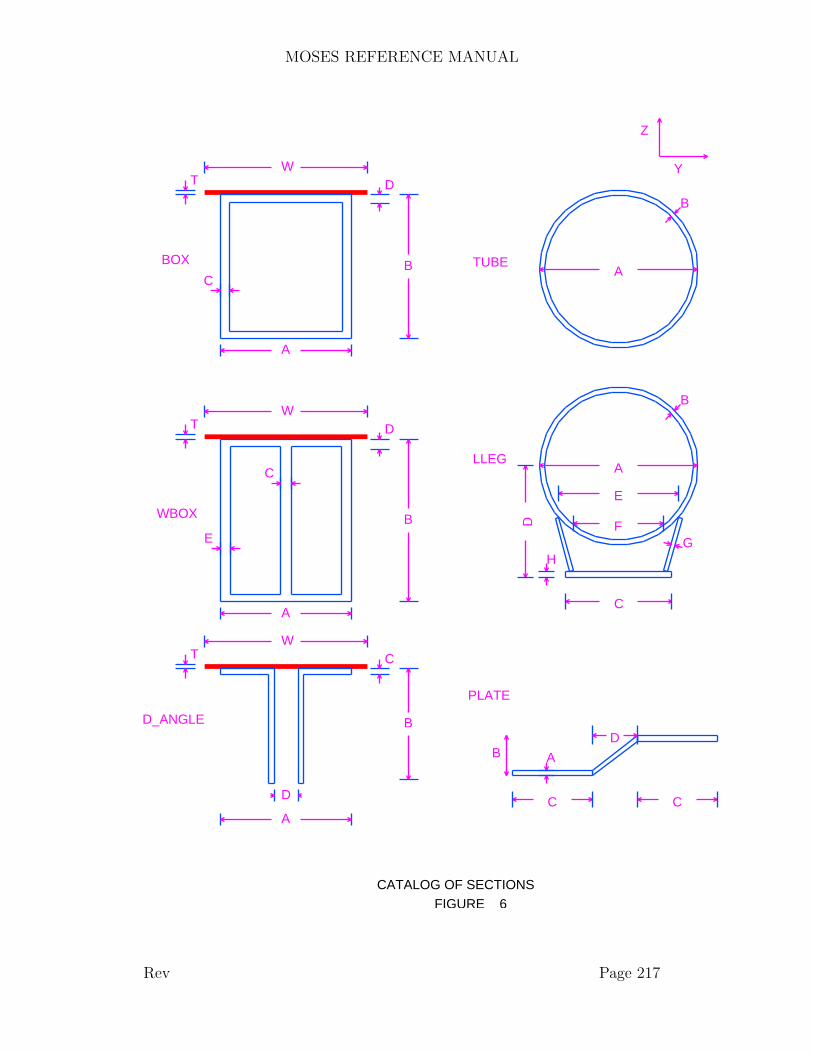
MOSES REFERENCE MANUAL
Y
Z
CATALOG OF SECTIONSFIGURE 6
BOX
TW
A
B
D
C
WBOX
TW
A
B
D
E
C
D_ANGLE
TW
A
B
C
D
TUBEA
B
LLEGA
B
C
H
D F
E
G
PLATE
C
A
C
DB
Rev Page 217

MOSES REFERENCE MANUAL
shear stresses into the true shear stresses at the neutral axis, i.e.
TAU(n) = ALPHA(n) * SHEAR FORCE / AREA
If any of these values are less than or equal to zero, the program computed value willbe used.
Normally, MOSES determines ”critical” points at which to compute stresses. Some-times, one wishes to define these points himself. Stress points are defined with the–POINTS option. Here, Y(n) and Z(n) are the beam system Y and Z coordinatesof the point and AY(n) and AZ(n) are the values of alpha for that point. (These arethe same alphas discussed above except that instead of computing the stresses at theneutral axis do it at the nth point.) The option –P FY allows one to define the yieldstress at the ”critical points”. If one uses this option, he really should define his ownpoints so that he is certain of the physical location of each point. The options –M Pand –P N define the plastic moments and the nominal axial strength of the section.NOTICE If you use the –SECTION option to change the properties, you probablywill also need to use the –M P and –P N options as well. The option –ETA definesthe exponent ”eta” in the interaction formulae of the AISC LRFD code check. Fi-nally, the option –F TYPE defines the fabrication type of the section. Here, TYPEmust be either FABRICATED or COLD FORGED.
The next class of Structural Class options are:
–LEN , L–PERL, PCLEN–REFINE, NUM REFINE–RDES, :NAME, KL/R LIM, D/T LIM
In general, MOSES allows for an element to have different properties along its length.To define such an element, one should have a Class definition command for eachsegment of the element. When more than one segment is defined, the first set ofproperties are associated with the beginning or ”A” end of the element, and the lastset of properties associated with the ”B” end of the element. The lengths of thesegments are defined by the –LEN option with L (feet or meters) being the length.For BEAM classes, the length of every segment but one should be defined. MOSESwill then compute the length of this segment so that the total length of the elementis correct. Also, one can define the segment lengths with the –PERL option. Here,PERL is the percentage of the total length of the element which will be attributedto a given segment.
When one uses a shape type of CONE, MOSES will automatically divide the beaminto a number of prismatic segments based on the number specified with the –
Rev Page 218
MOSES REFERENCE MANUAL
REFINE option. Thus, if –REFINE is not specified, then the beam will consist ofa single tube with a diameter which gives the correct volume. The thickness of theapproximate cylinder is
T = Ti * ( R1 + R2 ) / ( 2 * Ra )
where Ti is the thickness input, R1 and R2 are the radii at the ends and Ra is thediameter of the approximate cylinder. This is an approximation of the correct thick-ness for small values of (R1–R2)/L. Here, the first dimension given is the outsidediameter (inches or mm) at the ”beginning node” of the element, the second dimen-sion is the thickness (inches or mm), and the third dimension is the outside diameter(inches or mm) at the ”end node” of the element. The options which alter the loadattributes are not honored for cones, and one cannot use a cone section as the onewith zero specified length if when defining beams composed of different shape typesif the section is refined.
MOSES has an ability to automatically redesign a class of members so that all mem-bers within that class have favorable code checks. All resizing is performed on asubset of the shape table (more will be said about this in the next section). Thesubset considered during resizing is defined by a single selector, and two limits definewith the –RDES option. The program will consider only those shapes which matchthe selector. For tubes, only sections which satisfy the d/t and kl/r limits specifiedwill be considered. MOSES will consider all shapes selected to produce a shape whichwill yield a minimum cost and which satisfies the code check criteria.
MOSES allows one to define ”stiffeners” for structural elements. Both longitudinaland transverse stiffeners can be defined, and they add both stiffness and weight to amodel. In addition to adding weight and stiffness, stiffeners are used in checking somecodes. In general, stiffeners are associated with a previously defined class. The weightadded to elements by stiffeners can be eliminated with the use of the –ST USEWoption of either &DEFAULT or on the element definition command, or by specifying–WTPLEN to be zero when defining the stiffener class. The weight is computed bythe weight per length of the stiffener times its length times the number of stiffeners.If one does not specify a class for the stiffeners, then the stiffeners are ”magic” inthat they are weightless and automatically pass any checks on their properties.
While these are conceptually simple, one can easily become confused by the details.While the form of the options used to define stiffeners is the same for all elements,the details differ. Thus, let us begin by considering stiffeners on generalized plates.Here, the options used to define stiffeners are:
–T STIFF, SPACE, ∼STIF CLASS, WHERE
Rev Page 219

MOSES REFERENCE MANUAL
–L STIFF, SPACE, ∼STIF CLASS, WHERE
The option which begins with –T defines transverse stiffeners and that beginningwith –L defines longitudinal ones. Here, longitudinal stiffeners are parallel to theelement X axis and transverse ones are perpendicular to the X axis. For both ofthese, options, ∼STIF CLASS is the class name which will be used to define thestiffener, and have been defined previously. WHERE defines the ”vertical position”of the stiffener. WHERE may be either +Z, or –Z. If +Z is used, the stiffeners willbe connected to the ”top” size of the plate and for –Z, the bottom side. If WHEREis omitted, INTERNAL or +Z will be used.
Longitudinal stiffeners on beams are similar to longitudinal stiffeners on plates, andare defined with the –L STIFF option discussed above and
–LN STIFF, NUMBER, ∼STIF CLASS, WHERE
Also, here WHERE can also have the additional values of INTERNAL of EX-TERNAL which make sense for closed sections. In reality, +Z and EXTERNALare the same as are –Z and INTERNAL. The difference between –L STIFF and–LN STIFF is that the first defines the location of the stiffener by a spacing (hereSPACE is in inches or mm) and the second by the number of stiffeners. Obviously,
SPACE = DISTANCE / ( NUMBER + 1 )
Where DISTANCE is the distance over which the stiffeners are applied. For tubes,the distance is the circumference (inner or outer depending on WHERE). All othershapes are composed of rectangles. Here, DISTANCE and NUMBER are used foreach rectangle of the section and DISTANCE is the longer dimension. Thus, for a”PRI” section, the DISTANCE is the greater of A and B. Fractional stiffeners areused and they are ”smeared” over the full width. Thus, adding stiffeners increasesboth of the inertias of the section.
Transverse stiffeners on beams are the most complicated and are defined with eitherof the two options:
–T STIFF, SPACE, ∼STIF CLASS, WHERE, LENGTH–TN STIFF, NUMBER, ∼STIF CLASS, WHERE, LENGTH
Here, the values have the same meaning as those for longitudinal stiffeners on beams.The new value, LENGTH, will be discussed in a minute. One of the problems withtransverse stiffeners is that they are used for two purposes: stiffeners against hydro-static collapse and to stiffen joints. Since transverse stiffeners on beams are normallyused on tubes, we will call them rings here. To avoid confusion, rings will be used
Rev Page 220

MOSES REFERENCE MANUAL
to stiffen joints only if the class has more than one segment and the stiffeners are inthe segment closest to the joint}.
Transverse stiffeners suffer from the same problems as does buckling lengths. If anelement is not fully supported on both ends, then the longitudinal stiffener spacingmay be longer than the element length! This is where the value LENGTH comes in.It provides a ”DISTANCE” to be used in the conversion from spacing to number ofstiffeners. You can specify three things for LENGTH: a length in feet or meters, thetoken LENGTH, or the token BLENGTH. If LENGTH, is specified, the lengthof the element is used, if BLENGTH is specified, the minimum of the two bucklinglengths is used, a number input will be used directly, and if this parameter is omitted,the segment length will be used.
Let us consider two examples. First, suppose that we have an element which isactually part of a logical beam, and suppose the logical beam has a single hydrostaticring. If all elements of the logical beam had the same properties, they could be definedwith the class:
∼LBEAM TUBE OD T –TN STIFF 1 ∼SC EXTERNAL BLENGTH
This class will place one ring in the center of the logical beam and have a stiffenerspacing of half the minimum buckling length. Each element would have the samestiffener spacing, but a stiffer weight of the weight of the ring times the element lengthdivided by the buckling length. As another example, consider a beam for which weneed a joint ring at one end. The class
∼LBEAM TUBE OD T –TN STIFF 1 ∼JR EXTERNAL –LEN 2.5∼LBEAM TUBE OD T –TN STIFF 1 ∼HR EXTERNAL
We must use a segment to define the joint ring, hence the first segment. The hydro-static ring defined for the second segment will be the middle of the second segmentand the stiffener spacing here is half the length of the second segment.
Rev Page 221

MOSES REFERENCE MANUAL
XII.M.2 Class ShapesMOSES maintains a table of standard shapes. Here, a ”shape” is nothing more thana partial class definition. If one has an element made of one of these shapes, he cansimply specify it by SHAPE NAME. In other words, one can specify:
∼CLASS W14X140
and nothing else is required. Alternatively, one can now add any valid class optionto this definition to tailor it for his purposes. One can obtain a list of the currentlyavailable shapes by issuing &NAMES SHAPES. The basic table supplied with theprogram contains AISC, British, and French shapes.
One can add to the default shape table by entering a new menu with the command:
&DATA SHAPES
This command should be followed by records of the form:
NAME, TYPE, A, B, .... H –OPTIONS
where the available options are the section options discussed above:
–SECTION, AREA, IY, IZ, J, ALPHAY, ALPHAZ–POINTS, Y(1), Z(1), AX(1), AY(1), ..... \
Y(n), Z(n), AX(n), AY(n)–P FY, FY(1), FY(2), .... FY(n)–M P, Zy, Zz–P N, Pn–ETA, ETA–F TYPE, TYPE–T STIFF, SPACE, ∼STIF CLASS, WHERE–L STIFF, SPACE, ∼STIF CLASS, WHERE–TN STIFF, NUMBER, ∼STIF CLASS, WHERE–LN STIFF, NUMBER, ∼STIF CLASS, WHERE
Here, NAME is the name which one wishes to give the shape, and TYPE is a validclass section type (TUBE, CONE, BOX, PRI, WBOX, IBEAM, G IBEAM,TEE, CHANNEL, ANGLE, D ANGLE, PLATE, or LLEG), and A, B, etc.are dimensions (inches or mm) which are appropriate to define the shape.
When the shapes have been completely defined, one should issue END &DATAto exit. Normally, shapes defined via this menu are added to the basic shape tableprovided with the program, and remain defined only for the duration of a given
Rev Page 222

MOSES REFERENCE MANUAL
database. One can permanently add shapes to the basic table. To find out how toaccomplish this, look in the section on Customizing Your Environment.
For the AISC shapes, the standard names are used for most of the shapes. Theexceptions occur when the standard name exceeds eight characters. Jumbo W shapesare denoted by a J suffix. Angles are named Lddwwtt where dd is the depth in 1/10sof an inch, ww is the width in 1/10s of an inch, and tt is the thickness in 1/16s ofan inch. Double angles are named sLddwwtt where s is the spacing between the twoangles in 1/8 of an inch, dd is the depth in 1/10s of an inch, ww is the width in 1/10sof an inch, and tt is the thickness in 1/16s of an inch. Square and rectangular tubesare named TSddwwtt where: dd is the depth in inches, ww is the width in inches,and tt is the thickness in 1/16s of an inch. Here, exceptions are made for dd and wwvalues for some of the smaller sizes. For these tubes, dd and ww are in 1/10s of aninch.
For British shapes, names UdddBmmm are used for Universal Beams with depthddd (millimeters), and mass mmm (kilograms) per meter. Likewise, UdddCmmm isused for Universal Columns, UdddPmmm is used for Universal Bearing Piles, andJdddSmmm for Joists. The remaining shapes are named CdddBwww for channels,SHddttt for Square Hollow Sections, RHddwwtt for Rectangular Hollow Sections,LEdddttt for Equal Angles, and LUddwwtt for Unequal Angles. Here, dd denotes thedepth in centimeters, ww the width in centimeters, and tt the thickness in millimeters.
The French shapes in the table are denoted HEAZddd, HEAYddd, HEBZgddd,HEBYgddd, HEMZddd, HEMYddd, IPEZddd, IPEYddd, IPEZddd, and IPEYddd.Here, the shapes with the Z in their name are defined with the strong axis in thenormal direction while those with the Y in their name are rotated 90 degrees. Here,ddd is the depth of the section in millimeters.
The shape type of TUBE is special in that no plate can be attached to a tube.This shape also allows for having a tube inside of a tube, with the inside tube beingspecified by the dimensions C and D. If one has an inside tube, then he should notspecify contents for this element within this class. This is useful for defining pilesinside of legs.
Rev Page 223

MOSES REFERENCE MANUAL
XII.M.3 Pile ClassesA pile class is simply a beam class with a soil defined and some extra options available.The extra options for ∼CLASS PILE classes are:
–REFINE, NUM REFINE–PYMULT, PMUL, YMUL–TZMULT, TMUL, ZMUL–QWMULT, QMUL, WMUL–SOIL, SOIL NAME
The –REFINE option defines the number of segments into which the pile segmentwill be broken to solve the nonlinear pile/soil interaction problem. If it is omit-ted, a single element will be used. The options –PYMULT, –TZMULT, and–QWMULT define multipliers for the basic soil properties. If they are omitted,values of 1 will be used.
The option –SOIL defines the name of the soil in which the pile will be embedded.Here, SOIL NAME is the name of a soil which has been previously defined in the&DATA Menu. This is accomplished by first entering the menu with the command:
&DATA SOIL, SOIL NAME
and when the definition is complete, exit the menu with END &DATA. In themenu, one uses the following:
DEPTH, ZDISPY, P(1), Y(1), ......, P(n), Y(n)QW, Q(1), W(1), ......, Q(n), W(n)TZ, T(1), Z(1), ......, T(n), Z(n)MPY, MULP, MULYMQW, MULQ, MULWMTZ, MULT, MULZ
The basic rule here is that one first defines a depth. All of the properties then defined,until a new depth is encountered, apply to the specified depth. Here, ZDIS is thepositive distance from the mudline to point of interest (feet or meters). For pointsbetween two depths, a linear interpolation is performed, and for points outside thetable, the last closest point is used. The PY, QW, and TZ commands define theforce deformation behavior of the soil. Here,
• PY– defines the lateral behavior. P is the lateral force per unit length of pile(bforce/llength) which is required to produce a lateral deflection of Y (inchesor mm),
Rev Page 224

MOSES REFERENCE MANUAL
• TZ– defines the skin friction. T is the skin friction per unit length of pile(bforce/llength) which is required to produce a deflection on the pile surface ofZ (inches or mm),• QW– defines the end bearing. Q is the force (bforce) at the end of the pile
resulting from a vertical deflection of W (inches or mm).
The commands MPY, MQW and MTZ can be used to establish multipliers for thecurves. This is particularly important since all of the basic curves depend on pilesize. With these commands, the ith set of values will be multiplied by MULi beforethe data is stored in the database. As an example, if your PY data is given in tonnesand meters and your current units are kilo–newtons and meters, you could issue:
MPY, 1./1000, 1000.
and input the data as given.
Consider the following example:
∼PILE TUBE 1066.80 25.4 –DENSITY 77008.5 –SOIL DIRT \–REFINE 20 –FYIELD 360 –PYMULT 0.001
CONNECTOR PILE1 ∼PILE *J6110 *P110
Here, a tubular class is defined, the density is modified, the soil name is specified,and the pile is divided into 20 segments for a structural solution. The yield strengthand PY multiplier is also modified. This class definition is then used to describe aconnector, where *J6110 belongs to the part jacket, and *P110 belongs to the partground.
Rev Page 225

MOSES REFERENCE MANUAL
XII.M.4 Flexible Connector ClassesMOSES provides for several ways to flexibly connect bodies to one another or toground. These range from simple springs to assemblies of elements such as liftingslings and pipe assemblies. MOSES bases the definition of a connection on the typeof class defined for it.
To define an element with properties which vary along the length, one should definemultiple class commands with the same name. In contrast to beam and pile classes,every segment’s length must be defined for flexible classes. Also, the order of thesegments can be thought of as starting at the fairlead, moving toward the anchor.
There are three classes which define connectors with zero length, FOUNDATIONs,LMUs, and GSPRs. The class definition of these is:
∼CLASS, FOUNDATION, SENSE, DF(1), SPV(1), AF(1) ... \DF(n), SPV(n), AF(n), \
–OPTIONS∼CLASS, GSPR, SENSE, DF(1), SPV(1), AF(1) ... \
DF(n), SPV(n), AF(n), \–LEN, L, –OPTIONS
∼CLASS, LMU, LEN, OD(1), OD(2), \DF(1), SPV(1), AF(1) ... \DF(n), SPV(n), AF(n), \–OPTIONS
In addition to the standard class options discussed above, the following are, in general,available:
–SYMMETRIC, YES/NO–IG STIFF–SEND, KE(1), KE(2)–CONVOLUTION, CVL NAME–X PY, P(1), Y(1), P(2), Y(2), ......., P(n), Y(n)–Y PY, P(1), Y(1), P(2), Y(2), ......., P(n), Y(n)–Z PY, P(1), Y(1), P(2), Y(2), ......., P(n), Y(n)–X DAMPING, Co, Ex, Fo–Y DAMPING, Co, Ex, Fo–Z DAMPING, Co, Ex, Fo–FRICTION, MU
Here DF(i) is the name of the degrees of freedom (in the element system) whichwill be restrained and must be chosen from the list: X, Y, Z, RX, RY, RZ. By
Rev Page 226
MOSES REFERENCE MANUAL
default, the element system is aligned with the body system of the first node defininga connection. More will be said about this when defining elements are discussed.SPV(i) is the value of the spring (bforce/blength for degrees of freedom X, Y, and Z,and bforce–blength/radian for degrees of freedom RX, RY, and RZ) and AF(i) is theallowable force in this direction. For GSPRs and FOUNDATION elements, SENSEdefines the direction in which the element will act; i.e. if SENSE is TENSION,then the connector will have no load (in any degree of freedom) when the element Xdisplacement is negative. If SENSE is COMPRESSION then it will have no loadwhen the element X displacement is positive. The length here defines an elementX offset from the nominal beginning of the element to the spring. In reality, aFOUNDATION is simply a GSPR (generalized spring) which has zero length, andwill be checked in a FOUNDATION check. The –SYMMETRIC option can beused with connectors which are symmetric about the element X axis. If this option isused, then one should only define the ”Y” properties and MOSES will automaticallytake care of the rest. By default YES/NO is NO for GSPR and FOUNDATIONconnectors and YES for LMU connectors.
A LMU has geometry – a length and two diameters and is intended to model a pinin a cone. The cone and pin geometry are illustrated in Figure 7. Here, all threenumbers are in inches or mm. It too is a GSPR with a SENSE of COMPRESSION,but the deformation is not measured from the two points. It is best to think of thetwo point for the connector as the tip (bottom) of the pin and the ”top” of the cone.Let us define
T = ( OD(2) – OD(1) ) / ( 2 LEN )
Which is the tangent of the cone angle. Now, if the pin tip is above the cone top,then there will be no force. Now let D v be the distance the pin tip is below the conetop and D h be the horizontal distance that the pin tip is away from the cone center.If D v is less than LEN, then we will have a horizontal deformation given by:
Delta h = D h – T * ( LEN – D v )
If we assume that the force between the sides of the cone and the pin is perpendicularto the surface, then horizontal deformation will produce a vertical deformation
Delta v = –Delta h * T
Finally, if D v is greater than LEN the two deformations are
Delta v = D v – LEN – ( D h * T )
Rev Page 227
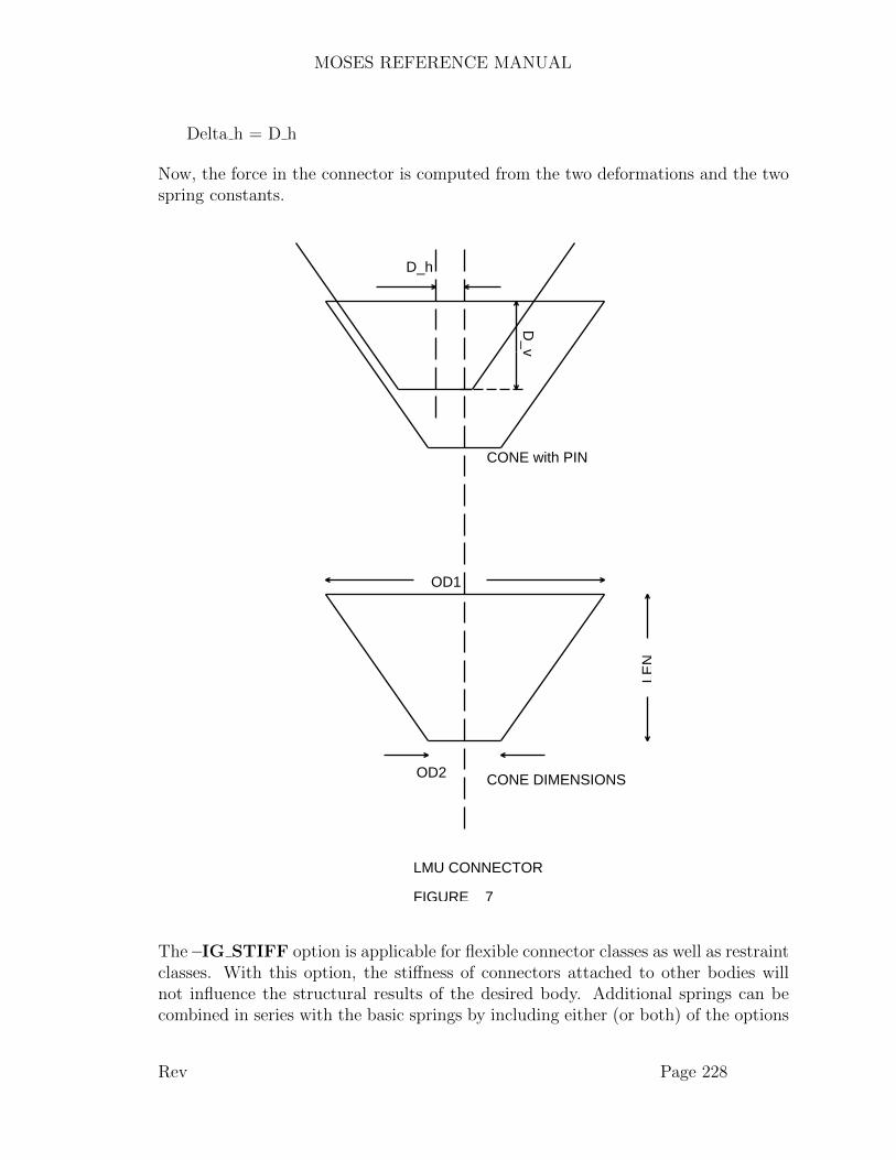
MOSES REFERENCE MANUAL
Delta h = D h
Now, the force in the connector is computed from the two deformations and the twospring constants.
CONE with PIN
CONE DIMENSIONS
LMU CONNECTOR
FIGURE 7
LEN
OD1
OD2
D_h
D_v
The –IG STIFF option is applicable for flexible connector classes as well as restraintclasses. With this option, the stiffness of connectors attached to other bodies willnot influence the structural results of the desired body. Additional springs can becombined in series with the basic springs by including either (or both) of the options
Rev Page 228

MOSES REFERENCE MANUAL
–SEND or –X PY. The first of these defines a nonlinear spring where the stretchin the spring, DEL, resulting from a force, F, is given by:
DEL = (KE(1) + F * KE (2)) * F.
The units for KE(1) are ft./kips, ft./l–tons, ft./s–tons, m/mt or m/kn and for KE(2),ft./kips**2, ft./l–tons**2, ft./s–tons**2, m/mt**2 or m/kn**2. The –CONVOLUTIONoption allows one to add an additional spring, but the behavior here is defined by aconvolution CVL NAME. This allows one to define springs that are viscoelastic aswell as elastic.
The –X PY, –Y PY and –Z PY options define nonlinear springs in series withthe basic x, y or z stiffness. Here, the letter following the – defines the ”element”degree of freedom to which the extra stiffness will be applied. All of these optionsdefine points on the force/deflection curve of a spring. Here, P(i) is the force inbforce, and Y(i) is the resulting deflection in feet or meters. The curve defined musthave the deflection being a function of the force. In other words, there can be no twopoints with the same P, and the points must be defined in increasing P. Also, MOSESassumes that the tension/compression behavior of the spring is the same so that thevalues should all be positive. Also, to avoid mathematical difficulties, Y should be amonotone increasing function of P.
The –X DAMPING, –Y DAMPING, and –Z DAMPING options defines anonlinear dashpot at the end of the element. As with the PY options discussed above,the letter following the – defines the degree of freedom in which these dashpots act.Here, the force is given by:
F = Co * ( v **Ex )
for F <= Fo (bforce). Here v is the relative velocity and Co is in (bforce–sec/ft orbforce–sec/meter). This dashpot is only active when the spring will have a force init.
The –FRICTION option can be used to limit the force in the element y and zdirections based on the element x force, and the precise behavior depends on thestiffness data. If either of the Y or Z stiffnesses are non zero, then friction is used asfollows. After the force components Fx and Fz have been computed, they are checkedagainst the product of Fx and MU; i.e. we compute
Fh = sqrt ( Fy*Fy + Fz*Fz )Fm = MU * abs ( Fx ) / Fh
Rev Page 229
MOSES REFERENCE MANUAL
FACT = min ( Fm, 1)
and then actually apply FACT * Fy and FACT * Fz. If both lateral stiffnesses arezero then the lateral force applied will be Fm and it will be applied in the directionopposite the relative velocity.
Three classes are used to define the constituents of slings and pipe assemblies:
∼CLASS, SLING, OD, –LEN, L, –OPTIONS∼CLASS, DAVIT, OD, –LEN, L, –OPTIONS∼CLASS, ROLLER, SENSE, DF(1), SPV(1), AF(1) ... \
DF(n), SPV(n), AF(n), \–OPTIONS
Slings and davits are similar in that they are really lines whose force depends onlyupon the distance between the ends. The cross–sectional area of these elements iscomputed from OD (inches or mm) assuming that the section is circular. The stiffnessis then given by AE and L (feet or meters). The only other option available for thisclass is –EMODULUS.
A ROLLER is a limited GSPR element. It is limited in that all of the optionsdiscussed above are not available. Here the available options are:
–Y PY , P(1), Y(1), P(2), Y(2), ......., P(n), Y(n)–Z PY , P(1), Y(1), P(2), Y(2), ......., P(n), Y(n)–Y ROLLER, Y–, Y+–Z ROLLER, Z–, Z+
If neither the –Y ROLLER nor the –Z ROLLER is specified, then the roller willautomatically restrain lateral motion and prevent the pipe from going below theroller. The values Y–, Y+, Z– and Z+ (inches or mm) define ”gaps” for the roller.Here a roller is assumed to consist of four physical rollers. A pair of these restrainmotion in each of the pipe system Y and Z directions. The Y– and Y+ values arethe dimension from the end of the connector to the physical roller. The same canbe said for the Z dimensions. To get a one sided constraint, use Z– equal 0 and Z+equal 10000. This says that the ”bottom” roller is at the connector node and the”top” roller is 10000 above the node. Since the pipe is unlikely to move this much,the top roller will never be active. All of these elements must have a single node, andthe second end will be taken care of in the assembly itself.
There are four classes which can be used to define a connector with finite length.
∼CLASS, ROD, OD, T, –LEN, L, \
Rev Page 230
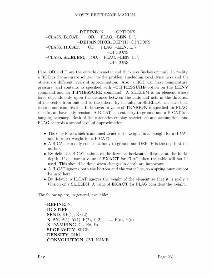
MOSES REFERENCE MANUAL
–REFINE, N, –OPTIONS∼CLASS, B CAT, OD, FLAG, –LEN, L, \
–DEPANCHOR, DEPTH –OPTIONS∼CLASS, H CAT, OD, FLAG, –LEN, L, \
–OPTIONS∼CLASS, SL ELEM, OD, FLAG, –LEN, L, \
–OPTIONS
Here, OD and T are the outside diameter and thickness (inches or mm). In reality,a ROD is the accurate solution to the problem (including local dynamics) and theothers are different levels of approximation. Also, a ROD can have temperature,pressure, and contents as specified with –T PRESSURE option on the &ENVcommand and an T PRESSURE command. A SL ELEM is an element whoseforce depends only upon the distance between the ends and acts in the directionof the vector from one end to the other. By default, an SL ELEM can have bothtension and compression. If, however, a value of TENSION is specified for FLAG,then is can have only tension. A B CAT is a catenary to ground and a H CAT is ahanging catenary. Both of the catenaries employ restrictions and assumptions andFLAG controls a second level of approximation:
• The only force which is assumed to act is the weight (in air weight for a H CATand in water weight for a B CAT).• A B CAT can only connect a body to ground and DEPTH is the depth at the
anchor.• By default,a B CAT tabulates the force vs horizontal distance at the initial
depth. If one uses a value of EXACT for FLAG, then the table will not beused. This should be done when changes in depth are important.• A H CAT ignores both the bottom and the water line, so a spring buoy cannot
be used here.• By default, a H CAT ignores the weight of the element so that it is really a
tension only SL ELEM. A value of EXACT for FLAG considers the weight.
The following are, in general, available:
–REFINE, N,–IG STIFF–SEND, KE(1), KE(2)–X PY, P(1), Y(1), P(2), Y(2), ......., P(n), Y(n)–X DAMPING, Co, Ex, Fo–SPGRAVITY, SPGR–DENSITY, RHO–CONVOLUTION, CVL NAME
Rev Page 231
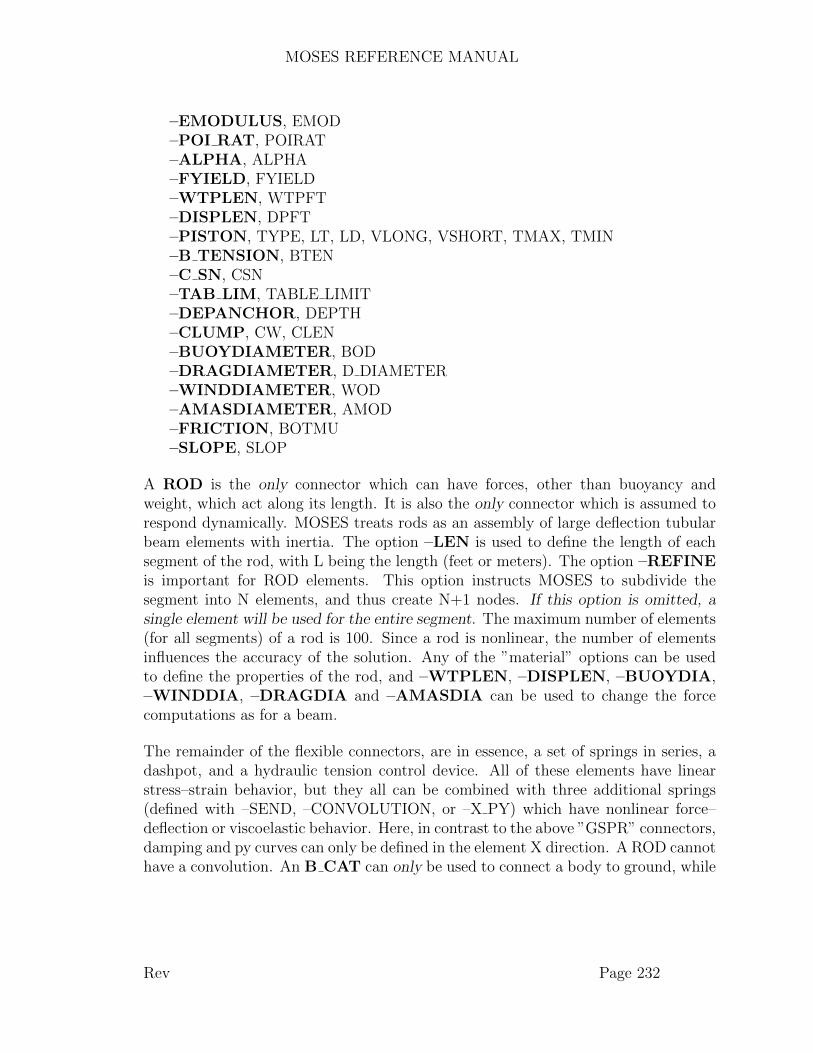
MOSES REFERENCE MANUAL
–EMODULUS, EMOD–POI RAT, POIRAT–ALPHA, ALPHA–FYIELD, FYIELD–WTPLEN, WTPFT–DISPLEN, DPFT–PISTON, TYPE, LT, LD, VLONG, VSHORT, TMAX, TMIN–B TENSION, BTEN–C SN, CSN–TAB LIM, TABLE LIMIT–DEPANCHOR, DEPTH–CLUMP, CW, CLEN–BUOYDIAMETER, BOD–DRAGDIAMETER, D DIAMETER–WINDDIAMETER, WOD–AMASDIAMETER, AMOD–FRICTION, BOTMU–SLOPE, SLOP
A ROD is the only connector which can have forces, other than buoyancy andweight, which act along its length. It is also the only connector which is assumed torespond dynamically. MOSES treats rods as an assembly of large deflection tubularbeam elements with inertia. The option –LEN is used to define the length of eachsegment of the rod, with L being the length (feet or meters). The option –REFINEis important for ROD elements. This option instructs MOSES to subdivide thesegment into N elements, and thus create N+1 nodes. If this option is omitted, asingle element will be used for the entire segment. The maximum number of elements(for all segments) of a rod is 100. Since a rod is nonlinear, the number of elementsinfluences the accuracy of the solution. Any of the ”material” options can be usedto define the properties of the rod, and –WTPLEN, –DISPLEN, –BUOYDIA,–WINDDIA, –DRAGDIA and –AMASDIA can be used to change the forcecomputations as for a beam.
The remainder of the flexible connectors, are in essence, a set of springs in series, adashpot, and a hydraulic tension control device. All of these elements have linearstress–strain behavior, but they all can be combined with three additional springs(defined with –SEND, –CONVOLUTION, or –X PY) which have nonlinear force–deflection or viscoelastic behavior. Here, in contrast to the above ”GSPR” connectors,damping and py curves can only be defined in the element X direction. A ROD cannothave a convolution. An B CAT can only be used to connect a body to ground, while
Rev Page 232
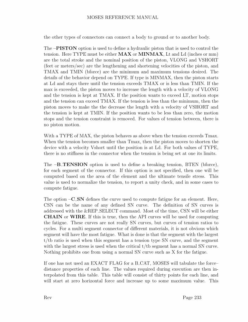
MOSES REFERENCE MANUAL
the other types of connectors can connect a body to ground or to another body.
The –PISTON option is used to define a hydraulic piston that is used to control thetension. Here TYPE must be either MAX or MINMAX, Lt and Ld (inches or mm)are the total stroke and the nominal position of the piston, VLONG and VSHORT(feet or meters/sec) are the lengthening and shortening velocities of the piston, andTMAX and TMIN (bforce) are the minimum and maximum tensions desired. Thedetails of the behavior depend on TYPE. If type is MINMAX, then the piston startsat Ld and stays there until the tension exceeds TMAX or is less than TMIN. If themax is exceeded, the piston moves to increase the length with a velocity of VLONGand the tension is kept at TMAX. If the position wants to exceed LT, motion stopsand the tension can exceed TMAX. If the tension is less than the minimum, then thepiston moves to make the the decrease the length with a velocity of VSHORT andthe tension is kept at TMIN. If the position wants to be less than zero, the motionstops and the tension constraint is removed. For values of tension between, there isno piston motion.
With a TYPE of MAX, the piston behaves as above when the tension exceeds Tmax.When the tension becomes smaller than Tmax, then the piston moves to shorten thedevice with a velocity Vshort until the position is at Ld. For both values of TYPE,there is no stiffness in the connector when the tension is being set at one its limits.
The –B TENSION option is used to define a breaking tension, BTEN (bforce),for each segment of the connector. If this option is not specified, then one will becomputed based on the area of the element and the ultimate tensile stress. Thisvalue is used to normalize the tension, to report a unity check, and in some cases tocompute fatigue.
The option –C SN defines the curve used to compute fatigue for an element. Here,CSN can be the name of any defined SN curve. The definition of SN curves isaddressed with the &REP SELECT command. Most of the time, CSN will be eitherCHAIN or WIRE. If this is true, then the API curves will be used for computingthe fatigue. These curves are not really SN curves, but curves of tension ratios tocycles. For a multi segment connector of different materials, it is not obvious whichsegment will have the most fatigue. What is done is that the segment with the largestt/tb ratio is used when this segment has a tension type SN curve, and the segmentwith the largest stress is used when the critical t/tb segment has a normal SN curve.Nothing prohibits one from using a normal SN curve such as X for the fatigue.
If one has not used an EXACT FLAG for a B CAT, MOSES will tabulate the force–distance properties of each line. The values required during execution are then in-terpolated from this table. This table will consist of thirty points for each line, andwill start at zero horizontal force and increase up to some maximum value. This
Rev Page 233
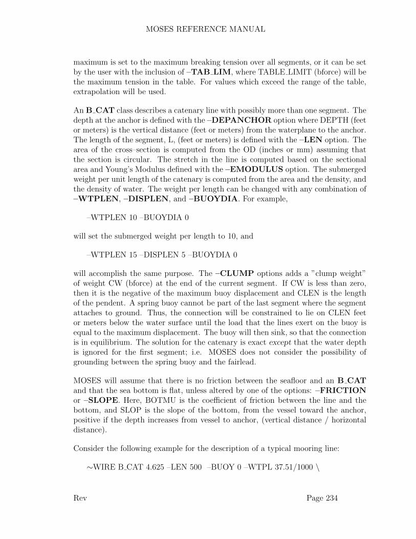
MOSES REFERENCE MANUAL
maximum is set to the maximum breaking tension over all segments, or it can be setby the user with the inclusion of –TAB LIM, where TABLE LIMIT (bforce) will bethe maximum tension in the table. For values which exceed the range of the table,extrapolation will be used.
An B CAT class describes a catenary line with possibly more than one segment. Thedepth at the anchor is defined with the –DEPANCHOR option where DEPTH (feetor meters) is the vertical distance (feet or meters) from the waterplane to the anchor.The length of the segment, L, (feet or meters) is defined with the –LEN option. Thearea of the cross–section is computed from the OD (inches or mm) assuming thatthe section is circular. The stretch in the line is computed based on the sectionalarea and Young’s Modulus defined with the –EMODULUS option. The submergedweight per unit length of the catenary is computed from the area and the density, andthe density of water. The weight per length can be changed with any combination of–WTPLEN, –DISPLEN, and –BUOYDIA. For example,
–WTPLEN 10 –BUOYDIA 0
will set the submerged weight per length to 10, and
–WTPLEN 15 –DISPLEN 5 –BUOYDIA 0
will accomplish the same purpose. The –CLUMP options adds a ”clump weight”of weight CW (bforce) at the end of the current segment. If CW is less than zero,then it is the negative of the maximum buoy displacement and CLEN is the lengthof the pendent. A spring buoy cannot be part of the last segment where the segmentattaches to ground. Thus, the connection will be constrained to lie on CLEN feetor meters below the water surface until the load that the lines exert on the buoy isequal to the maximum displacement. The buoy will then sink, so that the connectionis in equilibrium. The solution for the catenary is exact except that the water depthis ignored for the first segment; i.e. MOSES does not consider the possibility ofgrounding between the spring buoy and the fairlead.
MOSES will assume that there is no friction between the seafloor and an B CATand that the sea bottom is flat, unless altered by one of the options: –FRICTIONor –SLOPE. Here, BOTMU is the coefficient of friction between the line and thebottom, and SLOP is the slope of the bottom, from the vessel toward the anchor,positive if the depth increases from vessel to anchor, (vertical distance / horizontaldistance).
Consider the following example for the description of a typical mooring line:
∼WIRE B CAT 4.625 –LEN 500 –BUOY 0 –WTPL 37.51/1000 \
Rev Page 234

MOSES REFERENCE MANUAL
–EMOD 29000*0.1 –CLUMP –100∼WIRE B CAT 4.625 –LEN 4000 –BUOY 0 –WTPL 37.51/1000 \
–EMOD 29000*0.1∼WIRE B CAT 4.375 –LEN 2000 –BUOY 0 –WTPL 158.2/1000 \
–EMOD 29000*0.15∼WIRE B CAT 4.625 –LEN 2000 –BUOY 0 –WTPL 37.51/1000 \
–EMOD 29000*0.1 –DEPANCHOR 3000
Here, effort is saved by using minimum uniqueness and arithmetic in the input. Fourline segments are described, with a spring buoy at the end of the first segment.The first, second and fourth segments share the same material properties, except forlength. Notice the BUOYDIA is set to zero; therefore, the weight per length specifiedis the weight in water.
Rev Page 235

MOSES REFERENCE MANUAL
XII.M.5 Rigid Connector & Restraint ClassesRigid connector and restraint classes are defined by using one of the following:
∼CLASS, FIX, DF(1), ... DF(n),∼CLASS, SPR, DF(1), SPV(1), ... DF(n), SPV(n),∼CLASS, GAP, COEF
FIX and SPR classes define connections between specified degrees of freedom. Forthese connectors it is not permitted to define offsets. Instead, MOSES computes anoffset for the second end of the connection so that the constraint is satisfied whenthe connection is defined. Thus, one should issue an &INSTATE command for eachbody prior to connection to establish the proper relative orientation. The valuesinput when defining these classes are in the body system of the body to which thefirst node belongs. For both, DF(i) is the name of the degrees of freedom which willbe restrained and must be chosen from the list: X, Y, Z, RX, RY, RZ. A FIXclass will ”fix” the specified degrees of freedom of the element nodes. If all degrees offreedom are to be restrained, then one can simply specify FIX with no other values.The SPR class is used to define linear springs. Here, SPV(i) is the value of thespring (bforce/blength for degrees of freedom X, Y, and Z, and bforce–blength/radianfor degrees of freedom RX, RY, and RZ). These classes are used for defining bothrestraints and connectors. During a stress analysis, the behavior of a restraint and aconnector with the same class is identical. During a simulation, however, a connectorwill behave differently than one may expect. During a simulation, rigid constraintsare capable of restraining only translation. Thus, if one selects a rotational connector,it will only be applied during the stress analysis. Also, the connector applied duringa simulation will be the same regardless of whether FIX or SPR was used to definethe connection. The difference, however, will appear during the stress analysis wherethe specified flexibility will be applied.
A GAP connector is a rigid connector between two nodes. It will produce a forcebetween the two nodes acting from the second node to the first to keep the distancebetween them greater than or equal to the distance between them when the gap wasdefined. Notice that for a GAP connector to be properly defined, the two nodescannot be coincident. The vector from the second node to the first is called the gapdirection and the length of this vector when the gap was defined is called the gapdistance. The gap direction is considered to be a vector in the body to which the firstnode is attached. During a simulation, MOSES will compute the distance measuredalong the gap direction between the two nodes, and not allow this distance to be lessthan the gap distance. A gap cannot produce tension. If a gap has a specified frictioncoefficient, COEF, then it will behave differently during a simulation than during astress analysis. For the stress analysis, the treatment is according to Coloumb’s Law.For a simulation, a rigid connection is created perpendicular to the gap direction
Rev Page 236

MOSES REFERENCE MANUAL
whenever the gap is active, i.e. when the gap is active, it prevents all relative motionbetween the two points.
Rev Page 237
MOSES REFERENCE MANUAL
XII.M.6 Propulsion Connector ClassesIn MOSES, one can simulate the effect of a propulsion unit. These units have athruster and optionally, a rudder. A propulsion connector class is described using:
∼CLASS, PROPULSION, E NAME, MAX THRUST, R ALPHA, R GAMMA,R DIST
where the available options are:
–R ANGLE LIMITS, RA MIN, RA MAX–T ANGLE LIMITS, TA MIN, TA MAX
Here, E NAME is the name of an ”efficiency” curve and MAX THRUST is the max-imum thrust of the unit in bforce units. The thrust applied is the efficiency at therelative water particle velocity times the maximum thrust times the fraction of thrustapplied. The last factor and the thrust and rudder angles are defined with an optionon a &CONNECTOR command. The next three values define the optional rudder.R DIST is the distance (feet or meters) of the rudder shaft aft of the connector point.R ALPHA (ft**3 or m**3) and R GAMMA (ft**2 or m**2) define the force that isexerted normal to the rudder as
Fn = p * R GAMMAp = .5 * rho * s * vn
Here Fn is the force normal to the rudder, rho is the density of water, p is the pressure,s is speed the relative water velocity, and vn is the component of the relative velocitynormal to the rudder. The relative water particle velocity, v, is given by
v = vr + vtvt = abs ( thrust / ( .5 * rho * R ALPHA ) )
Here, vr is the relative water particle velocity in the absence of the thrust, and vt isthe water particle velocity induced by the thrust.
The options –R ANGLE LIMITS and –T ANGLE LIMITS are used to definelimits on the angles of the rudder and the thruster, and they should be between –90and 90. If no limits are given, then –90 and 90 will be used. The thrust fraction canbe between –1 and 1, so that by default the thruster can act in any direction. Fora thruster which can act in a fixed direction only, one simply limits the angles with–T ANGLE LIMITS.
Rev Page 238
MOSES REFERENCE MANUAL
XII.M.7 Tug Connector ClassesIn MOSES, one can simulate the effect of a tug boat attached to a body. Basically,this is a connector that applies a force in a constant global direction. When dynamicsimulations are considered, the force the tug applies varies with wave amplitude atthe tug position. A tug connector class is described using:
∼CLASS, TUG BOAT, FORCE
where the available options are:
–T DYNAM, PERCENT FORCE, PHASE–DAMPING, C
Here, FORCE is the force of the tug in bforce units. Statically, this force is simplythe amount specified. Dynamically, the force varies according to %FORCE, whichis the significant percentage of force change. PHASE is the phase angle in degrees,relative to the wave crest. This data is specified using the –T DYNAM option.The –DAMPING option defines a dashpot at the end of the tug with a constant C(bforce–sec/ft or bforce–sec/meter).
Rev Page 239
MOSES REFERENCE MANUAL
XII.N Structural Elements
In MOSES there are four types of structural elements: beams, generalized plates, partconnectors, and structural post–processing elements. All of the properties of theseelements are defined in terms of the ”element local system”. It is also the system inwhich loads and stresses will be reported. With respect to local system, the structuralpost–processing elements operate exactly the same as beams and generalized plates.The definition of the element system and the options that control it are considered inthe next section. All of the structural elements have additional attributes that canbe associated with them and which are defined with options. Most of these optionscan be used with any type of structural element and these are considered in a sectionbelow. Options which are specific to a given type of element are considered with theelement definition.
While one can alter existing elements by issuing a new BEAM or PLATE command,this is often cumbersome since all of the data must be redefined. An alternative isoffered by the command:
ED ELEMENT, OBJECT, –OPTIONS
where OBJECT is the name of the object to which the options will apply. If OBJECTis two node names (they may include wild characters, but must begin with an *),the attributes will apply to all beams between those two nodes. If OBJECT isan attribute class name (begins with a ∼), then the attributes will apply to allelements which belong to classes which match OBJECT. If OBJECT begins withneither an * nor a ∼, then the attribute will be applied to all members whose namesmatch OBJECT. Here, any option which is valid for the elements being edited canbe specified. The ED ELEMENT command works in the input channel throughINMODEL, or under the MEDIT menu.
The string function which returns information about an element is:
&ELEMENT(ACTION, DATA)
Where ACTION must be either EN NODES, CLASS, CATEGORY, ELE TYPE,STRW USE, WEIGHT, BUOYANCY, DCOSINES, BLENGTH, LENGTH,SEG LENG, RATIO, STRESS, CDR, NODES, RELEASES, E COORDINATES,OFFSETS, CFB, CM, KFACT, LAMBDA, HAS P–D and FLOODED, WIDTH,AREA, CENTROID, THICKNESS, SUBELEMENT, and DATA is normallyan element name. The first one, however, is different. Here, DATA is a set of nodenames and the data returned will be a list of element names all ends of which arein the set of node names. If one specifies only one node, then it returns all elementsconnected to the specified node. The remainder of ACTIONs take an element name
Rev Page 240

MOSES REFERENCE MANUAL
and return element information based on action. Most of these are obvious, for ex-ample the next four types of ACTION take an element name and the last computedunit check value, the last computed axial load, and the last computed cumulativedamage ratio.
The next set of options are applicable to all types of elements. The first of thesereturns the class name, the next the category name, and the next the element type.”BEAM” is returned for beams, ”PLATE” for plates, and ”OTHER” for anythingelse. STRW USE returns YES if the stiffener weight is included, NO otherwise.WEIGHT and BUOYANCY returns respectively, the weight and maximum buoy-ancy of the element. SN and SCF returns the SN curves used and the SCFs. Here,the order is from the first vertex to the interface between segments and finally the sec-ond vertex for a beam. For a generalized plate, there is only one value. DCOSINESreturns the 3X3 direction cosine matrix which transforms vectors in the element sys-tem into the part system. The next three option return element length and elementbuckling length, and the length of each segment in feet or meters respectively. Novalue is returned for SEG LENG when the element is a generalized plate.
The next three set of options are valid for beams and plates. The SN option returnsN values of SN where N is the number of segments plus one for a beam and one fora plate. The SCF option returns the SCFs used for beam fatigue. There are threetime the number of segments plus one for a beam and one number for plates. TheJ SCF option returns the eight SCFs used for joint fatigue at each end of the beamif both ends are parts of tubular joints. If an end is not part of a tubular joint, theNOT A TUBULAR JOINT will be returned for that end. If the end is part of atubular joint, but has the default values, then TUBULAR JOINT DEFAULTS willbe returned.
The next set of options are again valid for all types of elements. The next four optionsNODES, RELEASES, E COORDINATES, and OFFSETS, return the nodes,the releases (six values of YES or NO), the coordinates (three values in feet or meters),and the offsets (three values in inches or mm) at each vertex of the element.
The next set of the actions return values only for beam elements. CFB returns thecompression flange bracing in inches or mm and CM returns the CM factor used inthe AISC and API code checks. KFAC results the K factor used in the code checksand LAMBDA returns the strong and weak axis values of the slenderness param-eter. HAS P–D returns YES of the element includes p–delta loads, NO otherwise.FLOODED returns YES if the element is flooded, NO otherwise.
The last set of options return non empty values only for generalized plate elements.WIDTH, AREA, CENTROID, and THICKNESS Here, width and length are
Rev Page 241

MOSES REFERENCE MANUAL
the maximum distance (feet or meters) across the Y and X element axis respectively.The area is returned in ft**2 or m**2 and the centroid in feet or meters. The thicknessis returned in inches or mm. SUBELEMENT returns the subelement names forthe specified element excluding the base element itself. In other words, this actionwill return a null value for a triangular plate.
The string function which returns information about a subelement is:
&SUBELEMENT(ACTION, NAME)
Where ACTION must be either RATIO, STRESS, CDR, NODES, RELEASES,E COORDINATES, or OFFSETS, and NAME is the name of the subelement.The options here return the same data as the same one for the &ELEMENT stringfunction.
Rev Page 242
MOSES REFERENCE MANUAL
XII.N.1 Element SystemBoth beams and generalized plates have a special direction: along the length for abeam and normal for a generalized plate. Thus for a beam, the local X axis will befrom the first end to the second one, and for a plate the local Z axis will be normal tothe surface. One of the other two directions can be chosen arbitrarily and the thirdwill be defined by a cross product of the two vectors.
By default, MOSES has two additional vectors which will be used to complete thelocal system definition: a primary direction and a secondary one. Normally, theprimary direction defines the direction that an axis ”points”. For beams this is theZ axis, and for generalized plates it is the X. The secondary direction is used if thespecial direction and the primary direction are parallel. The primary and secondaryvectors, SAV1 and SAV2, are defined with the –DIR PLATE or –DIR BEAM optionsof a &DEFAULT command.
The SAV1 and SAV2 vectors are ”part system” vectors. This makes the business ofconnecting parts special since here one is dealing with two parts. The local systemof a part connector will be discussed below.
For a beam the local system is constructed as follows:
• If the beam X axis is not parallel to the SAV1 vector, then the beam Y axiswill be defined by the cross product of the SAV1 vector and the beam X axis.• If the beam X axis is parallel to the SAV1 vector, then the beam Y axis is
determined by the cross product of the SAV2 vector with the local X axis.
and for a generalized plate
• If the generalized plate Z axis is not parallel to the SAV1 vector, then thegeneralized plate Y axis will be defined by the cross product of the SAV1 vectorand the generalized plate Z axis.• If the generalized plate Z axis is parallel to the SAV1 vector, then the generalized
plate Y axis is determined by the cross product of the SAV2 vector with thelocal Z axis.
For both beams and generalized plates, the default behavior can be changed withtwo options on the element definition command:
–REFN, *REFNOD–DIR LOC, SAV1(1), SAV1(2), SAV1(3), SAV2(1), SAV2(2), SAV2(3)
The –REFN option replaces the default SAV1 vector with a unit vector from theelement origin (first point specified) to the point defined by *REFNOD. The –
Rev Page 243
MOSES REFERENCE MANUAL
DIR LOC option can be used to completely redefine both the SAV1 and SAV2vectors. If less than 4 numbers are specified with this option, then only SAV1 willbe redefined.
The local system definition described can be altered again for both beams and gen-eralized plates. In particular, for generalized plates, the –DIR LOC option can beused with only the string NODES following. This instructs MOSES to use the vec-tor from the local origin to the second node as the SAV1 vector. For beams, one canspecify the option:
–CA, CHANG
This option rotates the local system about the local X axis an angle of CHANG(degrees). The rotation of the system is about the beam x axis, positive towards thebeam negative Y axis (right hand rule).
If for a beam one wants the strong axis of beams to be ”horizontal”, the SAV1 vectorshould be the vector defining ”vertical” in the part system. In other words, if Z isthe part ”vertical” then SAV1 would be 0, 0, 1. Alternately if Y is the part ”vertical”then SAV1 would be 0, 1, 0. In either case, SAV2 simply handles the special caseand can be chosen to either suit one’s fancy or to conform to some existing practice.The relationship of the local coordinate system is shown in the following figure.
Rev Page 244

MOSES REFERENCE MANUAL
XII.N.2 Element OptionsIn general, the available options are:
–DIR LOC, SAV1(1), SAV1(2), SAV1(3), SAV2(1), SAV2(2), SAV2(3)–CA, CHANG–REFN, *REFNOD–SCFi, VALUES(1), ... VALUES(n)–SNi, CURVE–COLOR, NAME COL–TEXTURE, NAME TEX, X SCALE, Y SCALE–GOi, X, Y, Z–LOi, X, Y, Z–RELi, REL(1), REL(2), ..., REL(5)–CATEGORY, CAT NAME–USE, USE(1), USE(2), ..., USE(i)–NUSE, NOT USE(1), NOT USE(2), ..., NOT USE(i)–FLOOD, YES/NO–STW USE, YES/NO–NUM APPLIED, NUMBER
The options –DIR LOC, –CA and –REFN where discussed above, and for a discus-sion of the –SCF and –SN options, see the sections on associating SCFs AssociatingSCFs with Tubular Joints. and SN curves with fatigue points.
The options –COLOR and –TEXTURE define the color and texture of an element.These will be used when one asks for a picture with –COLOR MODELED. Here,NAME COL is any color which has been previously defined. See the section onColors for a discussion on defining colors. The NAME TEX value for –TEXTUREis the name of a file in either /X/data/textures or /X/data/local/textures (hereMOSES is store in /X). The X SCALE and Y SCALE are scale factors which will beapplied to the texture. The NAME TEX of NONE will yield a null default texture.
If one wishes to offset the vertices of an element from the nodes, he can employ oneof the options: –GO or –LO. The –GO options are used to define offsets at the”ith” vertex of the element. Here, –GO1 defines offsets at the first end, etc. Thevalues X, Y, and Z define the coordinates of the offset (inches or mm). For the –GOioptions, these coordinates are defined in the part system, while for the –LO options,they are defined in the member system. If only –GO, or –LO are specified, then allvertices will have the same offsets. In all cases, an offset is defined as the vector fromthe node to the vertex of the member.
Releases are governed by the options –REL. These options are used to define releasesat the ”ith” vertex of the element. Here, –REL1 defines releases at the first end,
Rev Page 245

MOSES REFERENCE MANUAL
etc. The values REL(i) define the particular releases to be applied. They must comefrom the list: FX, FY, FZ, MX, MY, MZ, but only as many as 5 may be specified.If –REL is specified, then all vertices of the element will have the same releases.
The loads due to the properties of the element are controlled with the options: –CATEGORY, –USE, –NUSE, and –FLOOD. The first three of these has beendiscussed with Categories and Load Types. If the –FLOOD option is used with aYES/NO value of YES, then a tubular member will be allowed to fill with waterif it’s below the water surface. Otherwise it will be assumed to be buoyant. Theoption –STW USE allows one to ”turn off” the weight of stiffeners. Here, YES/NOmust be either YES in which case the weight will be used or NO where the weightwill not be used. The option overrides the value set via &DEFAULT. The option–NUM APPLIED allows one to have a multiplier, NUMBER, for a beam. Theresults for a beam are first computed based on the specified properties, and thenall results are multiplied by NUMBER. In particular, the damping, stiffness, mass,matrices and the force are multiplied by this number.
Rev Page 246
MOSES REFERENCE MANUAL
XII.N.3 BeamsIn MOSES, an element is viewed as being the union of three sets of attributes: itsvertices, its class properties, and its ”additional attributes”. Defining the first two ofthese has already been discussed. To complete the definition of a beam, one uses:
BEAM, ELE NAME(1), ∼CLASS(1), –OPT(1), *NODE(1), ... *NODE(m), \ELE NAME(2), ∼CLASS(2), –OPT(2), NODE(n), ...
and in addition to the available options discussed above we have:
–CMFAC, CMY, CMZ–KFAC, KY, KZ–BLY, BUKLENY–BLZ, BUKLENZ–BLENG, BELE NAME–CFB, CFSPAC–HAS P–DELTA, YES/NO
BEAM defines a string of beams. Here, the ∼CLASS(i) defines the section at-tributes, and *NODE(1), *NODE(2), ...*NODE(n) is the list of connected nodeswhere, *NODE(1) connects to *NODE(2), *NODE(2) connects to *NODE(3), andso on. The locations of the command marked by –OPT(i) are positions where onemay place as many element options as desired, and may be omitted if defaults aresuitable for the beam in question. The beams from *NODE(1) to *NODE(m) havethe properties defined by ∼CLASS(1) and –OPT1, and the beams from *NODE(m)to *NODE(n) have properties defined by ∼CLASS(2) and –OPT(2). In other words,a beam in the string has the properties defined by the last ∼CLASS and/or –OPTdata issued before the beam was defined. Here, ELE NAME(i) is a name which canbe assigned to the element. If it is omitted, MOSES will assign a name. The ∼CLASSis a name for a set of element attributes which define the ”sectional properties”. Anexample of a beam definition accompanied by a sketch is shown in Figure 8.
The options specified above are used when checking codes. To alter the CM values foran element, one can use the –CMFAC option. Here, CMY is the factor for bendingabout the Y axis and CMZ is the factor for bending about the Z axis. The K factorsand the ”buckling lengths” are multiplied to obtain the effective length of the elementabout each axis. By default, the buckling lengths are taken to be the element lengthfor beams and the square root of the area for generalized plates. In particular, todefine the effective length multipliers for beams, one uses the option –KFAC. Here,KZ is used for bending about the Z axis, while KY is used for bending about the Yaxis. If this option is not used, both factors will be set to 1.
Element lengths for beams include the effect of any offsets, invoked by either the –GO
Rev Page 247

MOSES REFERENCE MANUAL
DESCRIPTION OF BEAM
FIGURE 8
Node *21 Node *22
762X25 762X19 762X25
3m 2m 2m 4m
&DEFAULT -FY 290~TUB762 TUBE 762 25 -LEN 2~TUB762 TUBE 762 19~TUB762 TUBE 762 25 -LEN 2BEAM ~TUB762 -LOA 3000 -LOB -4000 *21 *22
and –LO options on the BEAM card, or the –OFFSET option on the INMODELcommand.
The –BLENG or –BLY and –BLZ options can be used to alter the bucklinglengths about each axis. Here, the dimensions are feet or meters. The –BLENG,BELE NAME construct offers a way to ”bind” the buckling length of an element tothe load state of another element. Here, BELE NAME is the name of the ”braceelement”. If this option is exercised, then the KL factors of the basic element will bethose input if the brace element is in compression. If the brace element is in tension,then the factor for out of plane will be the same as for inplane. When this option isused, the ”compression” lengths will be used in any report or computation outsideof the Structural Post–Processing Menu. An alternative way of defining this type ofdependence is provided in the MEDIT Menu with the XBRACE command.
The –CFB option defines compression flange brace spacing, CFSPAC, (inches ormm). If this option is omitted, then the value will be taken to be the element length.Again, this is the length after accounting for any offset. The –HAS P–DELTAoption tells MOSES that this beam has nonlinear effects taken into account. IfYES/NO is YES then no interaction effects will be taken into account when thecodes are checked. If YES/NO is NO, or no option is used, then standard interactionformulae will be used in the code checking. For a tube, they are generally computed
Rev Page 248

MOSES REFERENCE MANUAL
based on the load path and the formulae specified. For other type sections, they areinput.
As an example of defining beams, consider:
∼STF TUBE 30 .75 –FY 42 –LEN 3∼STF TUBE 30 .675 –FY 42 –LEN 0.∼STF TUBE 30 .75 –FY 42 –LEN 3BEAM ∼STF –RELA MY –GO1 10 12 *AAA1010 *BBB1010
Here we have defined a single beam connecting the nodes *AAA1010 and *BBB1010,with properties defined by the class name ∼STF. The beam consists of 3 segments,hence the three STF commands. The first and third segments are tubular sectionswith 30 inch OD and 0.75 inch wall thickness, while the middle section has the sameOD, but only a 0.675 inch thickness. The first and third segments have a length of3 ft. and the length of the middle segment is to be computed by the program. Allsegments have a yield stress of 42 ksi.
As a second example, consider:
∼LONG, W18X40BEAM, ∼LONG, *A, *B
This defines 1 beam as a wide flange beam (18 x 40). This is a prismatic beam, asonly one ∼LONG command is given.
The example below uses a string of nodes for a beam description, which can sometimesbe quite useful:
∼TUBE TUBE 42 1.625BEAM ∼TUBE –GO1 10 10 10 *1 *2 *3 \
–GO2 12 12 12 *4 *5
In the above example, there are five nodes used, and four individual beam elementscreated. Each of the beam elements has a name assigned to it by MOSES. Theoptions apply in the order the beam is defined. For instance, *1 is the A end of thebeam joining nodes *1 and *2, and the –GO1 is a global offset at *1. *2 is the Aend of the beam joining nodes *2 and *3, with *3 as the B end of the beam. Thissequence continues for as many nodes as there are to define the entire series of beams.For the last beam of this series, *5 is the B end of the beam joining node *4 and *5,and the –GO2 option is a global offset at *5. The backslash (\) used above is for a
Rev Page 249

MOSES REFERENCE MANUAL
continuation of the same command on the next line.
In many instances, one needs to define beam load attributes other than those definedvia the element description. Three mechanisms for this are provided: two commandsand the –T PRESSURE option on the &ENV command and a T PRESSUREcommand. This option allows one to specify the temperature, internal pressure andthe density of the contents of a beam. The first of the command provided is:
#ELAT, OBJECT, WTPFT, DPFT, BOD, DOD, AMOD, WINOD –OPTIONS
and the available options are:
–TOTAL–CATEGORY, CAT NAME–A, XA–B, XB–LENGTH, LEN
This command is used to define additional intrinsic load attributes for a logical beam,and OBJECT is the name of the object to which they apply.
If OBJECT is two node names (they may include wild characters, but must begin withan *), the attributes will apply to all beams between those two nodes. Remember,there may be more than one beam defined between the same two nodes. Also, thesetwo selectors can be used to define load attributes on a ”logical” beam. For example,suppose that there is a beam between *1 and *2 and a beam between *2 and *3. Ifthese two beams are colinear, then #ELAT *1 *3 will apply the load to both beams.If OBJECT is an attribute class name (begins with a ∼), then the attributes willapply to all elements which belong to classes which match OBJECT. If OBJECTbegins with neither an * nor a ∼, then the attribute will be applied to all memberswhose names match OBJECT.
The data defines the attributes which will be added to the element. Here, WTPFTis a weight per foot (bforce/blength), DPFT is a buoyancy per foot (bforce/blength),BOD is the diameter (inches or mm) which will be used for buoyancy, DOD is thediameter (inches or mm) which will be used for viscous drag, AMOD is the diameter(inches or mm) which will be used for added mass, and WINOD is the diameter(inches or mm) which will be used for wind. With this command, one defines aline buoyancy with DPFT as well as a diameter which will be used for computingbuoyancy. Both can be used at the same time. The added mass and viscous dragcomputed will be based on Morison’s Equation. The –TOTAL option denotes thefact that the values input for WTPFT and DPFT are total quantities and should be
Rev Page 250
MOSES REFERENCE MANUAL
divided by the length to obtain the distributed properties.
By default, loads produced from the properties specified with #ELAT are assigned tothe default Extra Category. This can be changed with the –CATEGORY option.Also, the load attribute defined here will, by default, act over the entire length of theelements selected. If one wishes, he may alter this distribution with the options: –A,–B, and –LENGTH. Here, the attributes are defined over a segment of the originalbeam beginning XA (feet or meters) from the ”A” end of the beam, and extendingto XB (feet or meters) from the ”B” end, and the length over which it is appliedis LEN. The defaults are that both XA and XB are zero and LEN is the length ofthe beam. Thus, for a load over the entire beam, none of the option list is needed.Notice that the ”B” end of an attribute can be defined by either –XB or –LENGTH.Both should not be used on the same command.
The second command for beam attributes defines an applied load which belongs touser defined load set,
#LSET, OBJECT, VALA(1), .... VALA(6), –OPTIONS
and the available options are:
–VB, VALB(1), ... VALB(6)–LOCAL–TOTAL–A, XA–B, XB–LENGTH, LEN
Here, VALA(i), shown as FA, are the values of the attribute XA (feet or meters)from the ”A” end of the beam, and VALB(i), shown as FB, are the values at XB(feet or meters) from the ”B” end. If –VB is not specified, then the values at XBwill be taken to be the same as those at XA. The units for VAL(i) are in bforceand bforce–blength. To define an attribute in beam coordinates, one simply addsthe –LOCAL option. To input a concentrated attribute, one should specify LENto be zero. Figure 9 illustrates how the options are used. The –TOTAL commanddenotes the fact that the values input for VALA(i) and VALB(i) are total quantitiesand should be divided by the length to obtain the distributed properties. The options–A, –B, and –LENGTH operate in the same manner as the corresponding optionfor #ELAT and were discussed above.
Rev Page 251
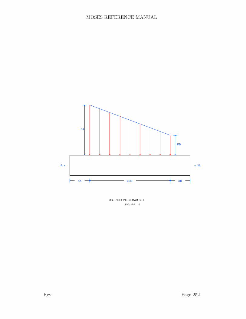
MOSES REFERENCE MANUAL
USER DEFINED LOAD SET
FIGURE 9
*A *B
FB
FA
XA XBLEN
Rev Page 252

MOSES REFERENCE MANUAL
XII.N.4 Generalized PlatesA generalized plate is a structural element defined with a set of nodes along theexterior, and perhaps, a set of points defining a free edge of the generalized plate.An edge of the generalized plate is the line segment between two adajent nodes onthe plate, and a ”face” is all edges which are on a line.
A generalized plate is defined with the command:
PLATE, ELE NAME, ∼CLASS, –OPTIONS, *NODE(1), *NODE(2), \*NODE(3), *NODE(4), ... *NODE(n)–FSOPT *FP(1), .......
This command defines a generalized plate element of class ∼CLASS, connected tonodes named *NODE(1) through *NODE(n). The nodes must be specified so asto go around the element in one direction. Here, ELE NAME is a name which canbe assigned to the element, omitted, MOSES will assign a name. The –OPTIONShave been discussed above. They may be omitted, or valid options may be inserteddirectly at this location within the command. The class name, ∼CLASS, is used tospecify the generalized plate’s attributes in exactly the same manner as for the beamelement.
A generalized plate is composed of subelements (triangular plates) contained withinthe defined perimeter, and can be any convex shape and some special concave ones.The number of subelements depends on the shape of the perimeter and the numberof nodes on each face. For three nodes you get no subelements and with four nodesyou get four subelements. If the generalized plate has four faces, the subelementsare generated as if it were composed of strips of quadrilateral elements. If not,the subelements are generated along rays (line segments from the average of thecoordinates of the specified nodes) to the nodes on the boundary. Subelements willbe generated so that the maximum distance of a side is less than or equal to themaximum distance between any two specified nodes. The internal nodes will havenames which begin with **IN. Figure 10 shows four typical generalized plates
and Figure 11 shows the corresponding subelements.
The –FSOPT options can be used to define concave generalized plates. Here *FP(i)are points which define a ”free edge”. The points define the geometry of the edge.The nodes on the other edges will determine where the nodes which will define thesubelements will be placed.
If –FSOPT is –HOLE then the free edge defines a hole contained within the gen-eralized plate and *FP(i) are points defining the geometry of the hole. Here *FP(1)
Rev Page 253
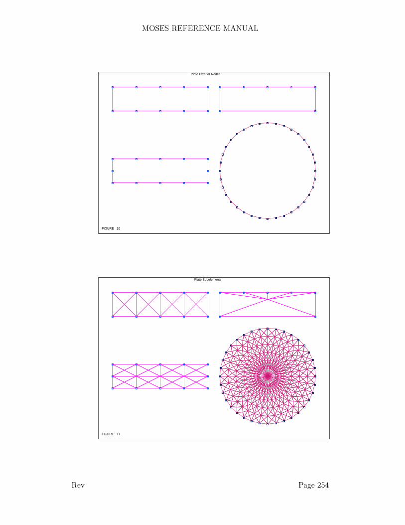
MOSES REFERENCE MANUAL
FIGURE 10
Plate Exterior Nodes
FIGURE 11
Plate Subelements
Rev Page 254
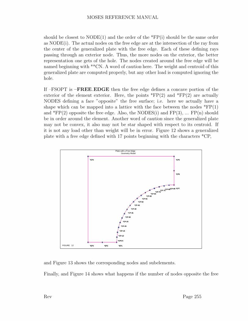
MOSES REFERENCE MANUAL
should be closest to NODE(1) and the order of the *FP(i) should be the same orderas NODE(i). The actual nodes on the free edge are at the intersection of the ray fromthe center of the generalized plate with the free edge. Each of these defining rayspassing through an exterior node. Thus, the more nodes on the exterior, the betterrepresentation one gets of the hole. The nodes created around the free edge will benamed beginning with **CN. A word of caution here. The weight and centroid of thisgeneralized plate are computed properly, but any other load is computed ignoring thehole.
If –FSOPT is –FREE EDGE then the free edge defines a concave portion of theexterior of the element exterior. Here, the points *FP(2) and *FP(2) are actuallyNODES defining a face ”opposite” the free surface; i.e. here we actually have ashape which can be mapped into a lattice with the face between the nodes *FP(1)and *FP(2) opposite the free edge. Also, the NODES(i) and FP(3), ... FP(n) shouldbe in order around the element. Another word of caution since the generalized platemay not be convex, it also may not be star shaped with respect to its centroid. Ifit is not any load other than weight will be in error. Figure 12 shows a generalizedplate with a free edge defined with 17 points beginning with the characters *CP,
FIGURE 12
*CP-10
*CP-15
*CP-20
*CP-25
*CP-30
*CP-35
*CP-40
*CP-45
*CP-50
*CP-55
*CP-60*CP-65
*CP-70*CP-75
*CP-80*CP-85
*CP0-5
*EP1*EP2*EP3
*EP4 *EP5
*EP6
*EP7
*CP-10
*CP-15
*CP-20
*CP-25
*CP-30
*CP-35
*CP-40
*CP-45
*CP-50
*CP-55
*CP-60*CP-65
*CP-70*CP-75
*CP-80*CP-85
*CP0-5
*EP1*EP2*EP3
*EP4 *EP5
*EP6
*EP7
Plate with a Free EdgeGeometry Model
and Figure 13 shows the corresponding nodes and subelements.
Finally, and Figure 14 shows what happens if the number of nodes opposite the free
Rev Page 255

MOSES REFERENCE MANUAL
FIGURE 13
**CN0026
*EP1*EP2*EP3
*EP4 *EP5
*EP6
*EP7
**CN0026
*EP1*EP2*EP3
*EP4 *EP5
*EP6
*EP7
Plate with a Free EdgeBasic Structural Model
edge is increased.
The only non–intrinsic load attribute one can specify for a generalized plate is atemperature specified with the –T PRESSURE option on the &ENV commandand a T PRESSURE command.
One can refine the edges of generalized plate elements with the command:
REFINE, MAX DIST, WHAT, SEL(1), SEL(2), .......
This command causes the edges of all generalized plates selected by the selectorsspecified to be refined so that the maximum length of an edge is MAX DIST (feet ormeters). Here WHAT can be either: EDGE, ELEMENT, or BOX. If one specifiesEDGE, the following SEL(i) should be in pairs of selectors; e.g. a pair *Q@ *R@ willselect any edge that has two nodes which match the two selectors. If one specifiedELEMENT, the following selectors select elements based on element name; e.g. QP@refines all edges of elements whose name matches QP@. Finally, a WHAT of BOXrefines edges which are totally with a box. Here, the values of SEL(i) should beX MIN, X MAX, Y MIN, Y MAX, Z MIN, and ZMAX. These are distances (feet ormeters) specified in the part system. Notice, all of these things can be used together.For example, one can have a BOX inside of a BOX with the interior one having asmaller MAX DIST. Then the interior one will have the interior MAX DIST and theexterior one the larger distance. The nodes added as a result of a refinement have
Rev Page 256
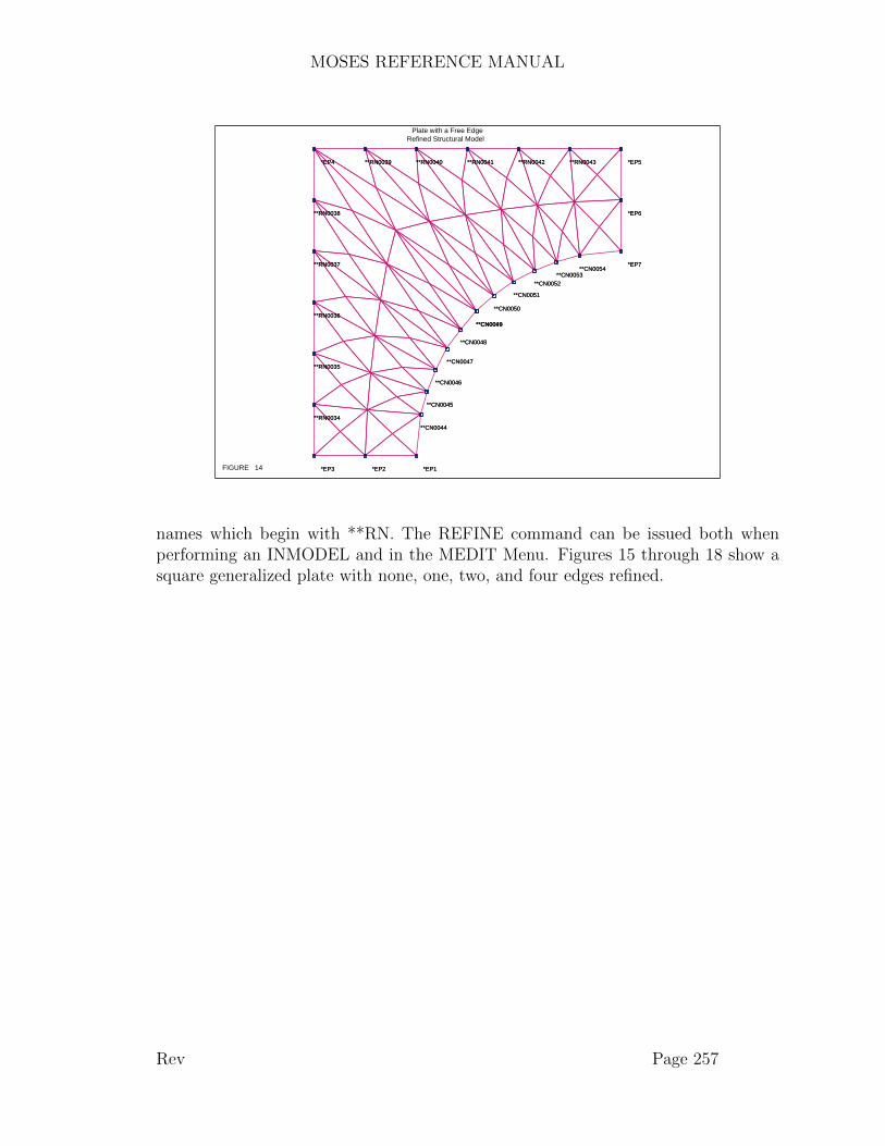
MOSES REFERENCE MANUAL
FIGURE 14
**CN0026
**CN0044
**CN0045
**CN0046
**CN0047
**CN0048
**CN0049
**CN0050
**CN0051
**CN0052**CN0053
**CN0054
**RN0034
**RN0035
**RN0036
**RN0037
**RN0038
**RN0039 **RN0040 **RN0041 **RN0042 **RN0043
*EP1*EP2*EP3
*EP4 *EP5
*EP6
*EP7
**CN0044
**CN0045
**CN0046
**CN0047
**CN0048
**CN0049
**CN0050
**CN0051
**CN0052**CN0053
**CN0054
**RN0034
**RN0035
**RN0036
**RN0037
**RN0038
**RN0039 **RN0040 **RN0041 **RN0042 **RN0043
*EP1*EP2*EP3
*EP4 *EP5
*EP6
*EP7
Plate with a Free EdgeRefined Structural Model
names which begin with **RN. The REFINE command can be issued both whenperforming an INMODEL and in the MEDIT Menu. Figures 15 through 18 show asquare generalized plate with none, one, two, and four edges refined.
Rev Page 257
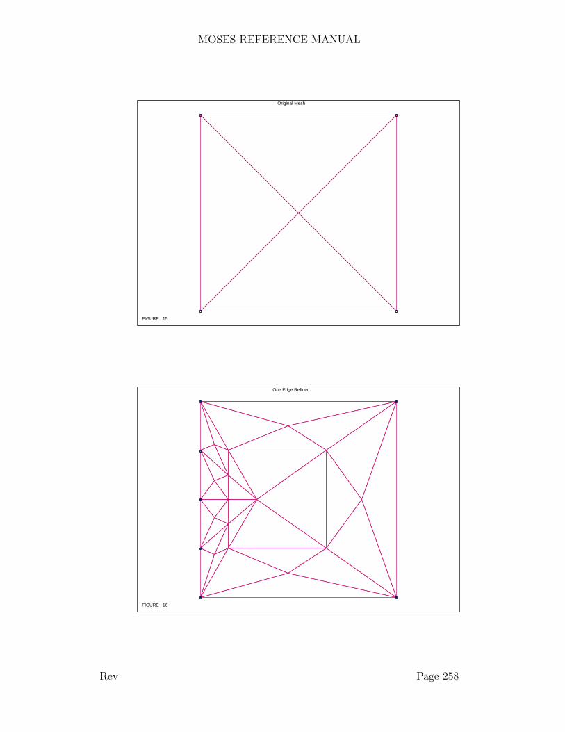
MOSES REFERENCE MANUAL
FIGURE 15
Original Mesh
FIGURE 16
One Edge Refined
Rev Page 258
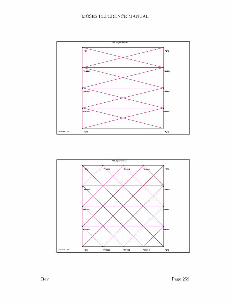
MOSES REFERENCE MANUAL
FIGURE 17
**RN0013
**RN0014
**RN0015
**RN0031
**RN0032
**RN0033
*QP1 *QP2
*QP3*QP4
**RN0013
**RN0014
**RN0015
**RN0031
**RN0032
**RN0033
*QP1 *QP2
*QP3*QP4
Two Edges Refined
FIGURE 18
**RN0013
**RN0014
**RN0015
**RN0031
**RN0032
**RN0033
**RN0038 **RN0039 **RN0040
**RN0041**RN0042**RN0043
*QP1 *QP2
*QP3*QP4
**RN0013
**RN0014
**RN0015
**RN0031
**RN0032
**RN0033
**RN0038 **RN0039 **RN0040
**RN0041**RN0042**RN0043
*QP1 *QP2
*QP3*QP4
All Edges Refined
Rev Page 259

MOSES REFERENCE MANUAL
XII.N.5 Connecting Parts
Connecting parts is a rather delicate proposition. Normally, the only elements whichdo not belong to a part are connectors. Connectors, however, are not designed tocarry moments and are not as general as beams. If, however, beams are allowedto span parts, their element system is not properly defined. Two alternatives areprovided to circumvent these difficulties. The first is that nodes can have an alias. Inother words, a node which has an alias will have the same deflection as the alternativename of the node. Defining a node alias is accomplished via:
ALIAS, *SLAVE(1), *MASTER(1), ...... *SLAVE(n), *MASTER(n)
When this command is issued, an element will be generated between *SLAVE(i) and*MASTER(i). No checking will be done as to the congruence of the locations of thetwo nodes, and these elements will not be used during simulations. Instead, theironly purpose is to insure that when a stress analysis is performed, the two nodes willhave identical deflections. One will normally use this technique to connect two nodesin different parts which have the same location in space.
The second method of connecting parts is with special connectors called part connec-tors. These elements belong to special parts which have a part type of PCONNECT.These elements may be defined by standard BEAM and PLATE commands, or theymay be defined in the MEDIT Menu by commands which are similar to the onesused in defining tiedowns. The additional commands are:
PCONNECT, ∼CLASS, *JN, :SEL(2)PCONNECT, DX, DY, DZ, ∼CLASS, :SEL(1), :SEL(2)
The first format generates part connectors at a single node in one part to severalnodes in the other part, using beams of section ∼CLASS. Thus ∼CLASS is the nameof the class property defining the section properties of the part connector member,*JN is the name of the node to be tied down, and :SEL(2) is a selector for the nodesto which *JN is connected.
The second format generates part connectors at several nodes, where the orientationof each part connector is constant. In effect, DX, DY, and DZ define the far end ofa beam element at each node which matches the selector :SEL(1). This far node isthen connected by a rigid link to the nearest node matching :SEL(2). Here, ∼CLASSis as before, and DX, DY, DZ is the distance measured from the node to the bodyattachment point, in the second part system (feet or meters).
A special method for connecting two parts for the transportation of a structure on avessel is provided by MOSES. To utilize this method, one must have a model which
Rev Page 260
MOSES REFERENCE MANUAL
consists of a single body with a body type of VESSEL, and there must be a partnamed JACKET with a part type of JACKET. This allows the part system of thejacket to be different from the vessel, and MOSES will automatically rotate the jacketso that the part systems are the same. Here, one must also establish connectionsbetween the parts so that an analysis can be carried out. The connections are oftwo basic types: launchways, which are continuous beams fastened to the vessel andupon which the jacket rests, and tiedowns, which fix the jacket to the vessel.
To use this feature, one should issue the command:
TRANS CON, –LOCJ, XO, YO, ZO, \–JLLEGS, *JS(1), ... *JS(n), \–JLLEGP, *JP(1), ... *JP(n), \–LWAYP, X1, ZNA, L, ∼CLASS, :BPSEL \–LWAYS, X1, ZNA, L, ∼CLASS, :BSSEL
The launchways are generated by the program as two continuous beams. Nodes onthese beams are automatically generated by MOSES to match up with the nodeson the jacket launch legs and with suitable nodes on the vessel. The jacket launchleg nodes are defined with the –JLLEGS and –JLLEGP options where *JP(i) arenodes on the port launch leg, and *JS(i) are nodes on the starboard launch leg. Inboth cases, the nodes must be ordered so that a given node is further aft than all ofthe nodes which precede it.
The jacket location on the vessel is given on the –LOCJ option where: XO, YO,ZO are distances (feet or meters), in the body system, from the vessel origin to thepoint midway between *JP(1) and *JS(1). With the jacket located on the vessel, thetwo launchways are defined using the –LWAYP and –LWAYS options. Here, X1 isthe vessel coordinate of the beginning of the launchway (feet or meters), ZNA is thevessel coordinate of the launchway neutral axis (feet or meters), L is the length of thelaunchway (feet or meters), ∼CLASS is the name of the class property defining thesection properties of the launchway, :BPSEL is a selector for the nodes to be rigidlyconnected to the port side (LWAYP) launchway, and :BSSEL is a selector for thenodes to be rigidly connected to the starboard side (LWAYS) launchway. Figure 19shows the effect of the above command.
To connect parts elastically, one employs tiedowns in one of two formats:
TDOWN, ∼CLASS, *JN, :SEL(2)TDOWN, DX, DY, DZ, ∼CLASS, :SEL(1), :SEL(2)
The first format generates tiedowns at a single jacket node which are connected usingbeams of section ∼CLASS to several vessel nodes. Thus ∼CLASS is the name of the
Rev Page 261
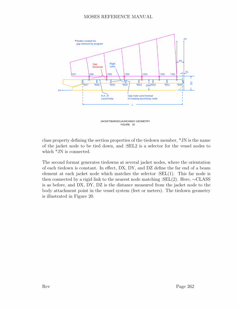
MOSES REFERENCE MANUAL
JACKET/BARGE/LAUNCHWAY GEOMETRYFIGURE 19
ZV
ZO
XV
ZNA
XO
X1
L
RigidLinks
*BS7 *BS6 *BS5 *BS4
Gap node used insteadof creating launchway node
*BS3 *BS2 *BS1 *BS0
GapElements
Nodes created forgap element by program
N.A. ofLaunchway
*JS7 *JS6 *JS5 *JS4 *JS3 *JS2 *JS1
class property defining the section properties of the tiedown member, *JN is the nameof the jacket node to be tied down, and :SEL2 is a selector for the vessel nodes towhich *JN is connected.
The second format generates tiedowns at several jacket nodes, where the orientationof each tiedown is constant. In effect, DX, DY, and DZ define the far end of a beamelement at each jacket node which matches the selector :SEL(1). This far node isthen connected by a rigid link to the nearest node matching :SEL(2). Here, ∼CLASSis as before, and DX, DY, DZ is the distance measured from the jacket node to thebody attachment point in the vessel system (feet or meters). The tiedown geometryis illustrated in Figure 20.
Rev Page 262
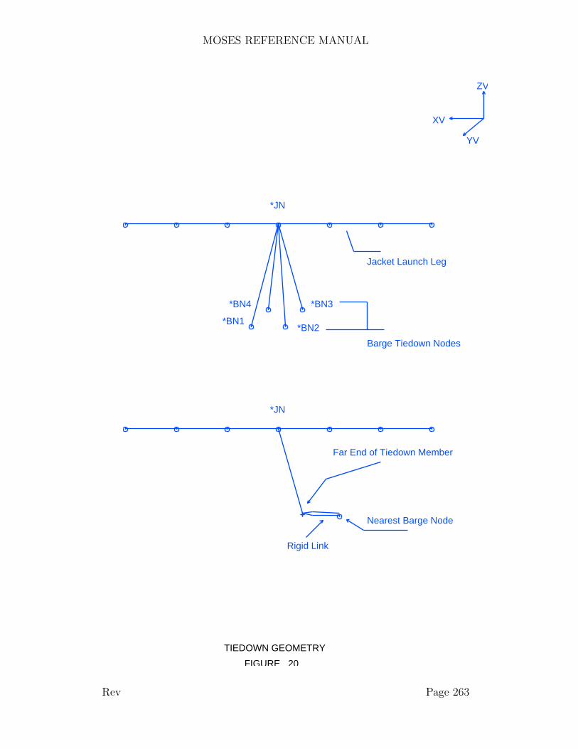
MOSES REFERENCE MANUAL
TIEDOWN GEOMETRY
FIGURE 20
XV
ZV
YV
*BN1
*BN4
*BN2
*JN
*BN3
Jacket Launch Leg
Barge Tiedown Nodes
Far End of Tiedown Member
*JN
Nearest Barge Node
Rigid Link
Rev Page 263

MOSES REFERENCE MANUAL
XII.N.6 Structural Post–Processing ElementsMOSES has a concept of ”pseudo elements” which can be used for structural post–processing. The pseudo elements are called sp beams or sp plates, and they aredefined in the same manner as beams or plates except that the command BEAM isreplaced with SP BEAM or PLATE is replaced with SP PLATE; i.e.
SP BEAM, ELE NAME(1), ∼CLASS(1), –OPT(1), *NODE(1), ... *NODE(m),\
ELE NAME(2), ∼CLASS(2), –OPT(2), *NODE(n), ...SP PLATE, ELE NAME, ∼CLASS, –OPTIONS *NODE(1), ... *NODE(m)
and there is an additional option which must be used:
–ELEMENTS, :ELSEL(1), .... :ELSEL(n)
These commands create a pseudo elements which have all of the properties definedwith their class and their geometry, but gets their load information from the ele-ments specified via the –ELEMENTS option. Here :ELSEL(i) are selectors for theelements which will be considered to ”be a part of” the SP BEAM or SP PLATE.
As mentioned above, these pseudo elements add nothing to the model – no stiffness,no weight, nothing. They are simply a useful way to look at parts of the model”in the large” for structural post–processing. In particular, suppose that one hada plate model of a semi–submersible. After a structural analysis, he has stresses inthe plates, but that is it. Now, to really analyze this situation, one needs to checkglobal buckling of the columns, etc. By creating SP BEAMS of the various pieces,this can be easily accomplished. For purposes of structural post–processing pseudoelements are treated the same as structural elements. Thus, one can also find bendingmoments and shears in them, stresses in them, etc.
Rev Page 264
MOSES REFERENCE MANUAL
XII.O Load Groups
The load group is a generalization of a nodal load. Here, a collection of load attributesis associated together as a group. For simulations, the load due to each of theattributes is computed and applied to the proper body. A load group also has a listof points associated with it. This list is given a name (normally the name of the loadgroup) and is called a load map. When a stress analysis is performed, the total loadon the group will be distributed to the nodes associated with the points by a leastsquares technique. Thus, if there is only one node associated with the group, it actsas a nodal load.
There are two primary differences between a load group and a nodal load. First,load groups allow for the association of not only loads, but also load attributes, withnodes. Secondly, the load attributes of a load group can be distributed to more thanone node. In addition to the obvious advantages of using attributes instead of loads,the load group allows one to define gross properties to entire bodies when he is notinterested in the structural details.
The load map may be either defined with a set of selectors as described below, orMOSES will define it for you. In particular, if one has not defined a map explicitly,the loads will be mapped to the points where load attributes have been defined.Whenever a body or part is defined, MOSES will automatically define a load groupwith the same name as the body or part.
Load groups are defined in much the same manner as bodies and parts. In otherwords, one issues:
&DESCRIBE LOAD GROUP, LG NAME, :NODE SEL(1), .. :NODE SEL(n),–OPTIONS
where the options are:
–DAMP FUSE, YES/NO–AMASS FUSE, YES/NO
and all load group attributes which follow belong to the specified load group. Here,LG NAME is the name which one wishes to give to the following load group, and:NODE SEL(i) are a set of selectors defining the points to which the loads will bemapped. The force from a load group is automatically distributed to the specifiednodes as if the nodes were connected to the point of application by a rigid structure.Note, however, the rigid structure is not required, since the force is distributed by aleast squares technique, as shown in Figure 21. The options –DAMP FUSE and –AMASS FUSE control the use of matrices defined with #AMASS and #DRAG
Rev Page 265
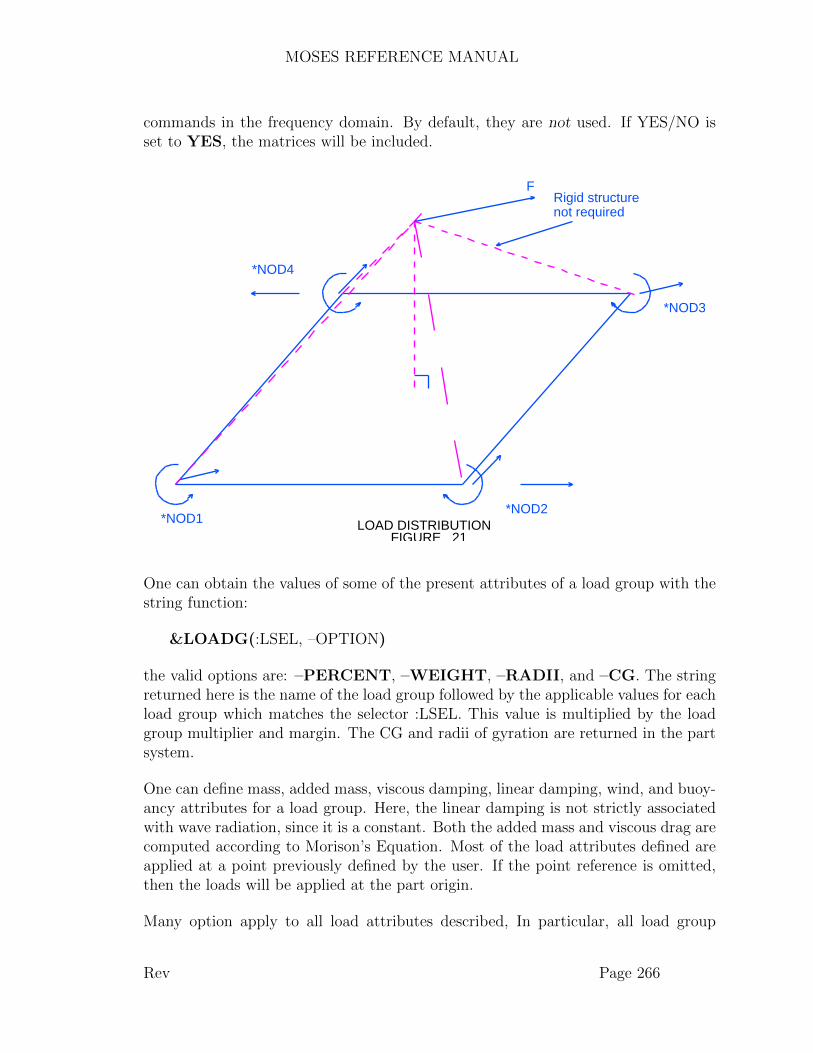
MOSES REFERENCE MANUAL
commands in the frequency domain. By default, they are not used. If YES/NO isset to YES, the matrices will be included.
LOAD DISTRIBUTIONFIGURE 21
F
*NOD4
*NOD3
*NOD2*NOD1
Rigid structurenot required
One can obtain the values of some of the present attributes of a load group with thestring function:
&LOADG(:LSEL, –OPTION)
the valid options are: –PERCENT, –WEIGHT, –RADII, and –CG. The stringreturned here is the name of the load group followed by the applicable values for eachload group which matches the selector :LSEL. This value is multiplied by the loadgroup multiplier and margin. The CG and radii of gyration are returned in the partsystem.
One can define mass, added mass, viscous damping, linear damping, wind, and buoy-ancy attributes for a load group. Here, the linear damping is not strictly associatedwith wave radiation, since it is a constant. Both the added mass and viscous drag arecomputed according to Morison’s Equation. Most of the load attributes defined areapplied at a point previously defined by the user. If the point reference is omitted,then the loads will be applied at the part origin.
Many option apply to all load attributes described, In particular, all load group
Rev Page 266

MOSES REFERENCE MANUAL
attributes are assigned a Category of the default ”extra” category by default. If onewishes to alter this, he may use the –CATEGORY option where indicated. Thus,one can have load attributes associated with different categories within the same loadgroup. Also, MOSES associates a multiplier with the load group as a whole. Thismultiplier may be changed as can the multipliers for categories with the &APPLYcommand. This allows one to be able to ”turn off” an entire load group as well asalter the force computations for some of the attributes.
Each of the attributes allows one to define a NUMBER, defined by an option, –NUM APPLIED, which multiplies the results of an attribute before it is applied.In other words, the force, mass, drag, and added mass are first computed based onthe properties defined. Then, each of these quantities are multiplied by the numberspecified before they are applied to the body.
The forces which will be applied are determined by a set of multipliers defined by the–WIND, –DRAG, and –AMASS options. These multipliers are similar to shapecoefficients in that a force is computed and then the multiplier is applied. If anyof these options are omitted, the corresponding multiplier is set to one. The forceswhich result from these commands are computed according to Morison’s Equation.Wind only acts on the area defined by #AREA if its center is above the watersurface. Similarly, water loads are only attracted when the center of area is belowthe water surface. –WAVE PM is used to define WAVMUL which is a multiplierfor wave particle velocity and acceleration. If WAVMUL is greater than zero, it isused to factor the wave particle velocity and acceleration before it is added to theother velocities and accelerations to compute a force. The default value of WAVMULis zero, in which case wave velocity and acceleration will not be considered for theload attribute.
The buoyancy due to these commands is defined by the –BUOY THICK option.Here, BTHICK is a thickness (inches or mm) which, when multiplied by the sub-merged area, will yield the buoyancy force.
Weight can also be defined with the other commands by using one or both of theoptions –TOT WEIGHT or –MULT WEIGHT. Here, WT is a weight, in bforce,which will be applied at the point of application. With the –MULT WEIGHToption, WMULT is a weight/area (bforce/blength**2) which is multiplied by the areadefined by either a #PLATE or a #AREA command to yield a weight applied atthe centroid. Both options can be used on the same command.
For any of the load attributes that follow, the options:
–TEXTURE, NAME TEX, X SCALE, Y SCALE
Rev Page 267

MOSES REFERENCE MANUAL
–COLOR, COLOR(1), FRAC(1), ... COLOR(n), FRAC(n)
can be used to define the color and texture of the attribute. These will be usedwhen one asks for a picture with –COLOR MODELED. Here, NAME COL is anycolor which has been previously defined. See the section on Colors for a discussionon defining colors. The NAME TEX value for –TEXTURE is the name of a filein either /X/data/textures or /X/data/local/textures (here MOSES is store in /X).The X SCALE and Y SCALE are scale factors which will be applied to the texture.The NAME TEX of NONE will yield a null default texture.
Perhaps the most popular of the load group class commands is the one which asso-ciates a weight with the group. The form of this command is:
#WEIGHT, *PT, WT, RX, RY, RZ, –OPTIONS
and the available options are:
–LDIST, X1, X2–NUM APPLIED, NUMBER–CATEGORY, CAT NAME
This command instructs MOSES that a weight of WT bforce is attached to the partat the location specified by the point *PT. This weight has radii of gyration RX,RY, and RZ (feet or meters) about the point *PT. The –LDIST option definesthe longitudinal distance over which the weight will be applied when computingtraditional longitudinal strength. Here, X1 and X2 are the beginning and endinglongitudinal coordinates (feet or meters) of the interval over which the weight will beapplied.
To define an applied force within a load group, one uses the command:
#LSET, *PT, FX, FY, FZ, MX, MY, MZ
This command defines an applied generalized force with the magnitude of the com-ponents given by FX, FY, etc. (bforce and bforce–blength). The force is appliedat the point defined by *PT, and is a member of the load set #LSET. As with alluser defined load sets, one must ”activate” the load set with an &APPLY commandbefore it will actually be applied.
To instruct MOSES to build an added mass matrix for the load group, one shouldissue:
Rev Page 268
MOSES REFERENCE MANUAL
#AMASS, *PT, DISP, CX, CY, CZ, RX, RY, RZ –OPTIONS
and the available options are:
–CATEGORY, CAT NAME
Here, the added mass will be DISP/G, where G is the gravitational constant. CX,CY and CZ are the added mass coefficients, and RX, RY, and RZ are added radii ofgyration, taken about the point specified by *PT.
Similarly, one can define a constant, linear drag matrix with the command:
#DRAG, *PT, DISP, D(X), D(Y), D(Z), R(X), R(Y), R(Z) –OPTIONS
and the available options are:
–CATEGORY, CAT NAME
Here, the force that will be produced is:
F(X) = DISP/G * D(X) * V(X)F(Y) = DISP/G * D(Y) * V(Y)F(Z) = DISP/G * D(Z) * V(Z)M(X) = DISP/G * R(X)**2 * OMEG(X)M(Y) = DISP/G * R(Y)**2 * OMEG(Y)M(Z) = DISP/G * R(Z)**2 * OMEG(Z)
Where G is the gravitational constant, DISP, D(i) and R(i) are the quantities spec-ified, V(i) is a velocity at the point *PT, and OMEG(i) is an angular velocity inrad/sec.
Point buoyancies can be associated with the load group by:
#BUOY, *PT, DISP, –OPTIONS
and the available options are:
–CATEGORY, CAT NAME–NUM APPLIED, NUMBER–TOT WEIGHT, WT
Here, DISP (bforce) is the magnitude of the buoyancy which will be applied. Again,this is applied at the location specified by the point *PT, and is applied only whenthis point is below the water surface. Weight can also be specified with this command
Rev Page 269

MOSES REFERENCE MANUAL
by use of the –TOT WEIGHT option. Here, WT is a weight (bforce) which willbe applied at the same point as the buoyancy.
The following two commands, #AREA and #PLATE, are somewhat similar inthat they both define an area which attracts water and wind forces. The format ofthe first of these is:
#AREA, *PT, AX, AY, AZ, –OPTIONS
and the available options are:
–CATEGORY, CAT NAME–NUM APPLIED, NUMBER–WIND, WINMUL–DRAG, DRGMUL–AMASS, AMSMUL–WAVE PM, WAVMUL–BUOY THICK, BTHICK–TOT WEIGHT, WT–MULT WEIGHT, WMULT
Here, AX, AY, and AZ (ft**2 or m**2) define the components of an area concentratedat the point specified by *PT.
In contrast to #AREA, a #PLATE command defines a distributed area, and loadattraction does not depend on the location of the center of area. The form of thiscommand is:
#PLATE, *PNT(1), *PNT(2), ............, –OPTIONS
and the available options are:
–CATEGORY, CAT NAME–NUM APPLIED, NUMBER–WIND, WINMUL–DRAG, DRGMUL–AMASS, AMSMUL–WAVE PM, WAVMUL–BUOY THICK, BTHICK–TOT WEIGHT, WT–MULT WEIGHT, WMULT
Here, one specifies up to four vertices of a polygon by points *PNT(i). These vertices
Rev Page 270
MOSES REFERENCE MANUAL
must be input in the order of one tracing the outline of the plate. MOSES willcompute the portions which are submerged and those which are above the watersurface, applying the proper forces in each regime. The level of detail used in the forcecalculation is defined by the –MAXAREA and –MAXREFINE and the methodof computing drag are defined with options of the &PARAMETER command. Theoptions for #PLATE function in the same manner as they do for #AREA, withone exception. When the submerged portion of a plate is computed, an aspect ratiois also computed. The added mass for the plate is that computed for a rectangularplate according to DNV Classification Notes 30.5.
Occasionally, it is convenient to describe a load attribute as a tubular, but withoutactually adding a tubular element to the model. This can be performed with thecommand:
#TUBE, OD, T, *PT1, *PT2 –OPTIONS
where the available options are:
–CATEGORY, CAT NAME–NUM APPLIED, NUMBER–WIND, WINMUL–DRAG, DRGMUL–AMASS, AMSMUL–WAVE PM, WAVMUL–TOT WEIGHT, WT–MULT WEIGHT, WMULT–BUOY DIA, BOD
Here, OD (inches or mm) is the diameter of the tube used to calculate environmentalforces and T (inches or mm) it the thickness. The tube is positioned between thepoints *PT1 and *PT2. The first eight options behave the same as for the #AREAcommand, and the –BUOY DIA option defines the diameter used to calculate buoy-ant forces for the attribute. The weight computed for this element is as describedabout for #AREA except that another weight is computed using the thickness, theOD, the current default density, and the length of the tube.
Wind and current forces can be input to MOSES and then associated with a loadgroup. This is achieved with the command:
Rev Page 271

MOSES REFERENCE MANUAL
#TABLE, T NAME, *PNT, –OPTIONS
Here *PNT is the point of application of the force and the available options are:
–WAVE PM, WAVMUL–CATEGORY, CAT NAME
When computing current forces, the wave particle velocity is computed a the mini-mum depth of the location of *PNT or the water surface. The wind speed is alwayscomputed at standard anemometer height so the wind is always allied regardless ofthe *PNT location.
For this command, T NAME is the name of a table of user defined force coefficientsfor wind and current. This table is defined using the &DATA menu:
&DATA A TABLE, T NAME, FLAG
where T NAME is the name of the force table. In this menu, the commands availableare:
ANGLE, ANG1WIND ARE, WAX, WAY, WAZ, WAMX, WAMY, WAMZCURR ARE, CAX, CAY, CAZ, CAMX, CAMY, CAMZ
The ANGLE, WIND ARE, and CURR ARE commands are repeated for eachangle, for up to 36 angles. If FLAG is specified as REFLECT, the angles specifiedshould range from 0 to 180 degrees. If this is not specified, the angles specifiedshould be from 0 to 360 degrees. These angles are either wind angles relative tothe body system, or relative body/current velocity angles. The body velocity usedis that computed at *PNT, specified in body coordinates as X, Y and Z. The forceacting at *PNT is calculated by multiplying the specified coefficients by the squareof the relative velocity. These force coefficients also create damping in the frequencydomain. For the WIND ARE and CURR ARE commands, X, Y and Z areforce coefficients, while MX, MY and MZ are moment coefficients. The prefix WAis for wind area, and CA is for current area. Remember to exit this menu usingEND &DATA.
If one wishes, he can associate a Tanaka Damping load attribute with a load group.This is accomplished with the command:
Rev Page 272
MOSES REFERENCE MANUAL
#TANAKA WETSUF –OPTIONS
and the available options are:
–ROLL, SECTION, FRACTION, BLOCK, DEPKEEL, KG, BEAM, BILRAD–PITCH, SECTION, FRACTION, BLOCK, DEPKEEL, KG, LENGTH, BIL-
RAD–PERIOD, T(1), T(2), ...., T(n)–ANGLE, AN(1), ...., AN(n)
The two options –ROLL and –PITCH are instructions to compute a set of Tanakadata and add it to what exists, and one can have up to 20 different occurrencesof these options. The degree of freedom which will be effected by the damping isdefined by the option name. Here, WETSURF is the total wetted surface of the body(ft**2 or m**2), and one can think of each pair of –ROLL and –PITCH optionsas defining the damping for a part of the body which has a fraction, FRACTION,of the wetted surface. All of the other variables for the option apply to the piecebeing defined. SECTION defines the type of section, and must be either BOW,MIDBODY or STERN. BLOCK is the block coefficient, DEPKEEL is the distancefrom the waterline to the keel (feet or meters), KG is the vertical center of gravityabove the keel (feet or meters), BEAM is the breadth of the body (feet or meters),LENGTH is the length of the body (feet or meters), and BILRAD is the bilge radius(feet or meters). No pitch damping is produced by default. If you define no additionaldata on the #TANAKA command, you will be put into a new submenu menu.
Once in the submenu, the equivalent linear damping coefficients are defined with thecommands
R TANAKA PER, VDM(1), ......, VDM(N)
or
P TANAKA PER, VDM(1), ......, VDM(N)
Here, PER is one of the periods specified with the –PERIOD option, and VDM(i)are the coefficients corresponding to the angles specified with –ANGLE. Noticethat VDM(1) corresponds to ANGL(1), VDM(2) with ANGL(2), etc. The units forVDM are bforce–sec–feet or meters. R TANAKA refers to roll damping coefficients,while P TANAKA is for pitch. This menu is ”exactly” the same as the one youhave before with I TANAKA.
The final command which can be used for defining load group attributes is differentfrom the others. Here, instead of defining specific load attributes, one defines the
Rev Page 273

MOSES REFERENCE MANUAL
wind and current load attributes of an entire vessel. The particular form of thiscommand is:
#TANKER, SIZE, TLEN, TDEP, TBEAM, AEX, AEY, LCP, –OPTIONS
and the available options are:
–CATEGORY, CAT NAME–CBOW–YAW FACTOR, YF–WAVE PM, WAVMUL
This command causes wind and current forces to be computed for a tanker of thespecified size according to the data presented in Prediction of Wind and CurrentLoads on VLCCs by the Oil Companies International Forum (OCIMF). NOTICE,these curves assume that the vessel is defined so that the X axis goes from bow tostern and that the keel of the vessel is at the origin of the part. These forces will beadded to any other forces computed for the load group. The option –CBOW shouldbe used if the tanker has a bulbous bow, and the option –YAW FACTOR controlsthe yaw viscous damping during a time domain simulation. The OCIMF formulaewere derived for computing the wind and current force on a stationary tanker. Insteadof simply using the current velocity in the formulae, MOSES uses the relative currenttanker velocity, so that viscous damping is obtained as well as applied force. Thisapproach works quite nicely for the basic forces and yaw moment, but produces zeromoment for a tanker which has zero velocity about the center of pressure regardlessof the yaw angular velocity. To overcome this problem, an additional term has beenadded which depends on the lateral coefficient and the yaw angular velocity. The–YAW FACTOR option specifies a multiplier for this extra term. A value of zerofor YF means that the term will not be used while a value of one means that it willbe used with no modification.
Here, SIZE is the size of the tanker in thousands of deadweight tons (e.g. a SIZE of100 would denote a 100,000 DWT tanker). If all of the other dimensions are omitted,they will be interpolated from an internal database. The other data are: length,depth, beam, extra frontal area, extra lateral area, and distance from the origin tothe longitudinal center of the tanker. Here the units are feet or meters for distances,and ft**2 or m**2 for areas. MOSES uses the major dimensions to compute thewind and current areas, and the extra areas are for wind only. There is an internaldatabase of default extra areas for AEX and AEY. These values are replaced when anon–zero value is used for AEX or AEY. In particular, the lateral wind area is givenby TDEP minus the draft times TLEN plus AEY. Likewise the frontal wind area is
Rev Page 274

MOSES REFERENCE MANUAL
(TDEP – DRAFT) * TBEAM + AEX.
In some cases, using #TANKER may cause forces in a direction opposite from oneexpects. This is a function of the OCIMF data, and not a problem with the software.There are lift forces involved with the ship shaped hull forms this data represents,sometimes causing this behavior. The OCIMF results are based on extensive windtunnel and tank tests on typical tankers. We have incorporated digitized versions ofthese curves into MOSES, therefore, what is derived is essentially what was measured.The question now becomes why are these forces in a direction opposite to what onemay expect – the answer is probably lift (but this depends on your expectations!), andis what permits us to sail and fly. The hull will behave like an aerofoil where the flowdoes not separate immediately at the bow (and particularly if it is cylindrical as faras wind loads are concerned). As a consequence, the longitudinal force componentsmay be ”negative”, i.e. up current or upwind, for some directions. Rest assured,however, the resultant force is always downweather so we can’t sail or fly for nothing– there is a net drag!
Rev Page 275
MOSES REFERENCE MANUAL
XII.P Compartments
Compartments are entities used for three purposes:
• To define hydrostatic, wind, and current forces on complicated shapes,• To define the sea/body interaction forces on things for which Morison’s Equa-
tion is not applicable, and• To define ballast in the interior of a body.
In essence, compartments are used to model the exterior of bodies and the interiorcompartmentation of bodies. Thus, we have two types of compartments: interior andexterior.
The distinction between interior and exterior compartments is made when the com-partment is named. Whenever a body is defined, MOSES will automatically definea compartment with the same name as the body. This compartment is an exteriorcompartment. Any other compartment defined whose name is not also the nameof some part is an interior compartment. Only exterior compartments can attracthydrodynamic loads, and only interior compartments can be flooded or ballasted.
Compartments are a collection of two basic entities: pieces and tube tanks. A tubetank is used to model the interior of a tube, and pieces are used to model everythingelse. In essence, a piece is a ”ship like” part of the compartment. When a pieceis part of an exterior compartment it creates buoyancy, drag force, wind force, andbehaves according to either Strip Theory, Three Dimensional Diffraction Theory, orattracts no hydrodynamic load at all. When part of an interior compartment, it canbe damaged (flooded) or ballasted and defines part of the inertia of the system. Theway to define pieces and tube tanks will be discussed below.
Compartments are defined in a fashion similar to bodies and parts. In other words,the data for a compartment follows an &DESCRIBE command naming the com-partment:
&DESCRIBE COMPARTMENT, CNAME –OPTIONS
Here, CNAME is the name of the compartment and the options define additionalattributes for interior compartments and will be discussed later.
Tube tanks are a computationally efficient way to define interior compartments. Theonly restriction is that the physical shape defined by a tube tank must be a circularcylinder. A given compartment can have as many tube tanks as desired, and each
Rev Page 276

MOSES REFERENCE MANUAL
one is defined by:
TUBTANK, DIA, PNT(1), PNT(2)
Here, DIA is the diameter (inches or mm) of the tank and PNT(1) and PNT(2) arethe names of two points defining the ends of the tank. Alternately, the coordinates ofthe ends (feet or meters) can be input instead of point names. If one uses coordinates,points will be defined with these coordinates. These tanks can be mixed with otherpieces for an internal compartment. If one attempts to define a tube tank for anexterior compartment, an error will result.
Rev Page 277

MOSES REFERENCE MANUAL
XII.P.1 PiecesFor more complicated geometries, compartments are defined with pieces. In essence,a piece is a closed surface in space. Each piece is, in turn, defined by a set of connectedareas called ”panels”. Both interior and exterior compartments can be composed ofas many pieces as required. There are two basic ways to define a piece: by definingeach panel, or using a more powerful language to generate the panels. In the nextsection, an even more powerful method of generating panels by Boolean operationson existing pieces will be discussed.
In addition to geometry, pieces have several additional attributes, all of which aredefined as options on the command which defines the piece. Here, we will first discussdefining pieces via panels and then turn to the easy way. A panel description of apiece begins with the command:
&DESCRIBE PIECE, PIECE NAME, –OPTIONS
and the available options are:
–PERMEABILITY, PERM–OBSTACLE,–DIFTYPE, TYPE–CS WIND, CSW X, CSW Y, CSW Z–CS CURRENT, CSC X, CSC Y, CSC Z–CS VELOCITY, CS VELOCITY NAME–DD MULT, DDR(1), MULT(1), ...., DDR(n), MULT(n)–AMASS, AMA MULT, AM CURVE–TANAKA, TANAKA FACTOR–ROLL DAMPING, ROLL DAMP FACTOR–COLOR, COLOR(1), FRAC(1), ... COLOR(n), FRAC(n)–TEXTURE, NAME TEX, X SCALE, Y SCALE
Here, PIECE NAME is the name of the piece. If this is omitted, a name will beautomatically generated by MOSES. The –PERMEABILITY option can be usedto alter the buoyancy of a piece. Here, PERM is the permeability of the piece,and it should be positive for a buoyant piece and negative for a hole or a floodedcompartment. A value of one corresponds to 100 percent of the piece’s volume.The default value for permeability is 1 for an exterior piece, and –1 for an interiorcompartment.
The –OBSTACLE option provides a method for defining an obstacle in the water,with which a floating body will have hydrodynamic interaction. The obstacle belongsto the body defined with the last &DESCRIBE BODY command, but does notmove in a simulation. Multiple obstacles may be defined, so that several situations
Rev Page 278

MOSES REFERENCE MANUAL
may be analyzed. For instance, three obstacles may be defined and arranged to simu-late a floating body inside a dry dock. A single obstacle can be arranged underneatha body to represent a sloping sea floor. It is important to note that an obstaclewill move only when the body it is attached to moves as a result of a positioningcommand, such as &INSTATE –LOCATE.
The remaining options of the PIECE command are applicable only to exterior com-partments and are used to define how forces on the piece will be computed. The–DIFTYPE option defines which hydrodynamic theory will be used for the piece.Here, TYPE must be either 3DDIF if one wishes to use Three Dimensional Diffrac-tion Theory, or NONE if the piece is to be ignored in computing hydrodynamicproperties. If one wants to use Strip Theory, he must define the piece with a PGENcommand which is discussed later. The –CS WIND and –CS CURRENT optionsdefine how the panels of the piece attract wind and current loads.
In general, for each panel in a piece, MOSES will split it into a portion above thewater and a portion below. The wind force on the out of water portion and the currentforce on the below water portion are computed as if the area was a #PLATE. Here,however, the components of the velocity are multiplied by the values of CSC X,CSC Y, and CSC Z respectively. In addition, the current force is multiplied by amultiplier, MULT, that depends on the water depth to draft ratio, DDR. This valueis obtained by interpolation from the table defined with the –DD MULT option.The default values for the CSs and the multiplier table are set with the &DEFAULTcommand.
Several other things need to be said here. First, the ”current” force actually dependson both the current velocity and the velocity of the panel, so using the word currentis really incorrect. Second, the results are quite dependent upon the setting of –AF ENVIRONMENT option of &PARAMETER. If the option is set to NOand the above is used for ”round” pieces, the results may be surprising. The forceproduced for a rectangular box is exactly the same as one would get by using a pairof #PLATEs. For a circular cylinder, however, one gets a force of .785 (pi/4) timesthat of a square box. This is simply a result of the recipe used to compute the force.Thus, to get ”the correct” force on a cylinder, one should specify:
–CS WIND .5/.785 .5/.785 1–CS CURRENT .5/.785 .5/.785 1
If the setting is YES then this does not apply.
The option –CS VELOCITY can be used to change the first component of theCS CURRENT values. Here, CS VELOCITY NAME is the name of a ”curv” whathas been defined with the command CS VELOCITY with the command &DATA
Rev Page 279
MOSES REFERENCE MANUAL
CURVE CS VELOCITY. If this option is used, then the relative speed at each panelwill be used to interpolate a drag coefficient.
The –AMASS option defines a multiplier for an estimate of the added mass of apiece. If the name AM CURVE is omitted, then MOSES will estimate the addedmass in these three directions as a function of submergence. These estimate arebased on the projection of the ”box” containing the submerged piece onto the bodycoordinates for surge and sway and on the waterplane for heave. Here you will getthree polygons, one for each coordinate direction. The added mass in each directionis obtained as if this polygon is an isolated plate. If AMA MULT is zero, no addedmass will be accumulated for this piece. The slopes of the heave curve are also usedto compute slam loads in heave. If you wish, you can define a ”curve” with a type ofAM PRESSURE with the command &DATA CURVE AM PRESSURE. Notice thatthis is an excellent way to estimate added massed for isolated plates and for thingswhich will change their submerged shape considerably, but it should be turned offfor pieces which are used for diffraction or strip theory hydrodynamics.
The option –TANAKA defines a multiplier for the damping due to ”eddy making”.In MOSES, we refer to this as ”Tanaka” damping after the person who first formulatedthe results for eddy making damping. In MOSES, we use the formulation outlinedin a paper by Schmidke in The Transactions of the Society of Navel Architects andMarine Engineers (1978). The default value here is defined by an option of the samename for the &DEFAULT command. The option –ROLL DAMPING definesa quadratic damping factor, ROLL DAMP FACTOR in ( sec**2 – feet or meters –bforce )/rad**2. When defined, it applies a roll moment given by:
roll moment = ROLL DAMP FACTOR * omega**2
and omega is the roll angular velocity. CAUTION if either of these option are usedin conjunction with –CS CURRENT then roll will be over damped.
The –COLOR and –TEXTURE options can be used to define the color and tex-ture of the piece. These will be used when one asks for a picture with –COLORMODELED. Here, NAME COL is any color which has been previously defined. Seethe section on Colors for a discussion on defining colors. The NAME TEX value for –TEXTURE is the name of a file in either /X/data/textures or /X/data/local/textures(here MOSES is store in /X). The X SCALE and Y SCALE are scale factors whichwill be applied to the texture. The NAME TEX of NONE will yield a null defaulttexture.
The string function:
Rev Page 280

MOSES REFERENCE MANUAL
&PIECE( ACTION, NAME )
can be used to return information about a piece. Here, NAME is the piece aboutwhich information is desired and ACTION must be either CURRENT, PAN-ELS, DIFTYPE, PERMEABILITY, CS WIND, CS CURR, AMASS, LO-CATION, or OBSTACLE, and the type CURRENT returns the current piecename, PANELS returns the names of the panels in the specified piece, and all of theothers return the data defined with the options of the same name.
After the piece has been defined, its geometry is defined by a set of convex polygonscalled panels. Each panel is defined by points at its corners with the command:
PANEL, PAN NAME, PTNAM(1), ....., PTNAM(n)
Here, PAN NAME is the optional name assigned to the panel, and PTNAM(i) arenames of its vertices. If PAN NAME is omitted, a panel name will be assignedinternally. A panel can contain from three to fifty vertices. The order of the definitionof the vertices should be clockwise when the panel is viewed from outside of the body.In other words, the normal to the surface when defined by the right hand rule shouldpoint into the body. One can alter this convention by using the command,
REVERSE, –OPTIONS
and the available options are:
–YES–NO
The counterclockwise order for the vertices should be used following a REVERSE–YES command. If one wishes to change back to the basic convention, he shouldthen issue REVERSE –NO.
The string function:
&PANEL(ACTION, NAME )
can be used to return information about a panel. Here, NAME is the panel aboutwhich information is desired and ACTION must be AREA, NORMAL, E COORDINATES,PERIMETER, or G CENTROID. These return the obvious things with E COORDINATESreturning the part coordinates of the ends and G CENTROID returning the globalcentroid.
While the above method is certainly general in that all possible surfaces can be
Rev Page 281
MOSES REFERENCE MANUAL
defined as accurately as desired, actually defining a mesh with panels can becomequite tiresome. As an alternative, MOSES provides a menu for ”generating” a piece.This menu begins with the command:
PGEN, PIECE NAME, –OPTIONS
and the available options are:
–PERMEABILITY, PERM–OBSTACLE,–DIFTYPE, TYPE–CS WIND, CSW X, CSW Y, CSW Z–CS CURRENT, CSC X, CSC Y, CSC Z–CS VELOCITY, CS VELOCITY NAME–DD MULT, DDR(1), MULT(1), ...., DDR(n), MULT(n)–AMASS, AMA MULT, AM CURVE–TANAKA, TANAKA FACTOR–ROLL DAMPING, ROLL DAMP FACTOR–COLOR, COLOR(1), FRAC(1), ... COLOR(n), FRAC(n)–TEXTURE, NAME TEX, X SCALE, Y SCALE–STBD–PORT–BOTH–TOL OFF, TOL–LOCATION, X, Y, Z, ROLL, PITCH, YAW
and ends with an END PGEN command. Here, most of the options are exactlythe same as those for the PIECE command, and the last five define how to interpretthe plane data which will follow.
In this menu, the closed surface of the piece will be defined as a sequence of polygonscalled planes. In contrast to panels, these planes do not define the surface directly,but define ”cuts” through it. To proceed, consider two coordinate systems, a localsystem used in this menu only, and the part system. The local X axis lies along thelength of the piece, positive aft. The local Z axis is perpendicular to the local Xaxis, and is positive ”up”. The local y axis is defined by the local X and Z axes,and the right–hand rule (positive to starboard.) The surface of the piece is nowdefined by its intersection with a set of planes. These planes have constant local Xvalues and the intersection is defined by a set of local points, (Yi,Zi). The optionsdefine how the points will be interpreted. The default is to define only the positiveY portion of the plane, allowing MOSES to automatically produce the negative half.If one specifies –STBD, no reflection will be performed. If –PORT is specified,then the plane is reflected, and the positive portion is deleted. Finally, if –BOTH
Rev Page 282
MOSES REFERENCE MANUAL
is specified, one must define both halves of the plane. In this case, one first definesthe positive portion and proceeds around the contour to define the negative portion.In all cases, one starts at the bottom of the station (minimum z and zero y) andproceeds around counter clockwise (point 2 is has non decreasing z from point 1).If using Strip Theory, the user should set TYPE to be STRIP and the –STBD,–PORT and –BOTH options cannot be used. The –CS options work exactly thesame as described above.
The –TOL OFF option allows one to omit offsets which lie on a line from the model.This is often desirable since MOSES gives the correct answers for planes of any size.Here, TOL is the cosine in the angles minus 1 which will be considered to be colinear.
The –LOCATION option allows one to place and orient the generated piece withrespect to the part system. The position of the piece is defined by X, Y, and Z (feetor meters). These are the part coordinates of the origin of the local coordinates ofthe piece. The orientation of the piece is defined by the three angles: ROLL, PITCH,and YAW. These are defined as follows: Suppose that the piece is given successiverotations about the local Z axis, then about the new local Y axis, and finally, aboutthe new local X axis, so that the piece, after the three rotations is in its properorientation in space. These three angles can be thought of as a yaw, followed by apitch, followed by a roll to move the piece from when it is aligned with the globalsystem to its required position in space.
In this menu, the actual definition of the surface is accomplished by a set of com-mands:
PLANE, X(1), X(2), ...., X(n), –OPTIONS
and the available options are:
–RECTANGULAR, ZBOT, ZTOP, BEAM, NB, NS, NT–CARTESIAN, Y(1), Z(1), Y(2), Z(2), ......, Y(n), Z(n)–CIRCULAR, Y, Z, R, THETA, DTH, NP–E CIRCULAR, Y, Z, R, THETA, DTH, NP
where: X(i) is a local X coordinate of the plane (feet or meters), and the offsets ofthe section are defined by the options. The X values for a piece must be defined innon–decreasing order; i.e. one should not have
PLANE 10 –10 ...
If the section is rectangular, it can be completely defined by one –RECTANGULARoption. Here: ZBOT is the local Z coordinate of the bottom of the section (feet or
Rev Page 283
MOSES REFERENCE MANUAL
meters), ZTOP is the local Z coordinate of the top of the section (feet or meters), andBEAM is the width of the section (full width, feet or meters). Normally, the sectionis defined with 4 points, but this can be changed with the values NB, NS, NT. NBdefines the number of points along the bottom, NS the side, and NT the top. Forother types of sections, the –CARTESIAN, –CIRCULAR, or –E CIRCULARoptions are used. With the –CARTESIAN option Y(i), Z(i) are local Y and Z co-ordinates of the ith offset point (feet or meters). The –CIRCULAR option allowsone to input data in polar coordinates. Here: Y and Z are local coordinates of thecenter of the circle (feet or meters), R is the radius of the circle (feet or meters),THETA is the angle of the first point (degrees) measured from the negative localZ axis positive toward Y, DTH is the increment in angle (degrees), and NP is thenumber of points to be generated. It is important to notice that any number of–CIRCULAR and –CARTESIAN options can be used to define the section. The–E CIRCULAR option is the same as the –CIRCULAR option except that theradius which is specified is not the one which will be used. Instead, a new radius willbe computed so that the area of the polygon defined by the new radius is the sameas that of the circular sector.
The number and size of the panels determine the accuracy of the results. Of course,the computational effort required is quite sensitive to the number of panels and so oneis constantly seeking a good compromise between fidelity and efficiency. Complicatingthis, however, is the fact that there are several different things for which accuracyis important. The algorithm which computes hydrostatic results from the mesh is”exact” in that the results obtained from a given mesh are the same as those obtainedfrom a refined mesh for the same body. Thus, from a pure hydrostatic point of view,the most desirable mesh is the coarsest one which properly defines the surface of thebody.
In a structural analysis, however, a different problem arises. By default, the structuralloads on a panel are mapped to the nodes closest to the vertices of the panel. If youhave a large number of nodes in comparison to the number of panels, then the defaultwill not yield a good load distribution. If the default scheme is to work properly,then there should be a reasonable relationship between structural nodes and cornersof panels. In other words, if one has a single panel for the side shell of a barge, heshould at least have points on the panel at each longitudinal location where he hasstructural nodes.
To eliminate many of these difficulties, MOSES has a command available in theMEDIT menu:
Rev Page 284
MOSES REFERENCE MANUAL
M PAN FIX, TOL OP, TOL B, –OPTIONS
where the available options are:
–BOUNDARY–NODES, YES/NO–COMPART, :CMP SEL–PIECE, :PIECE SEL–PANEL, :PAN SEL–POINTS, :PNT SEL–X, X BOX1, X BOX2–Y, Y BOX1, Y BOX2–Z, Z BOX1, Z BOX2–DIRECTION, DIR
The purpose of this command is to change the nodes to which the loads will bemapped for selected panels. The details of the options will be addressed later. Thetwo numbers TOL OP and TOL B control the remapping. To see how these work,consider the situation discussed above. In particular, suppose that you have largepanels and small plates, so that there are several plates which are inside a panel.By default, there will be no load applied to the nodes at the vertices of the interiorgeneralized plates. M PAN FIX will solve this problem by adding points on theboundary and interior of the panel to the list of points which will receive the load.Here, TOL OP (feet or meters) defines an out of plane tolerance. Only points withinTOL OP distance along the normal of the plane will be considered. Likewise, TOL B(feet or meters) defines a boundary tolerance, and only points with a distance ofTOL B of the boundary will be considered to belong to the boundary. These twotolerances define what is meant by ”on the boundary” and ”inside the panel”. If apoint is within TOL B of the boundary in the plane of the panel and within TOL OPof the plane of the panel, then it is ”on the boundary” of the panel. If a point is”inside” the panel (a distance greater than TOL B away from the boundary andinside the panel) and within TOL OP of the plane of the panel, then it is insidethe panel. If the –BOUNDARY option is used, all points inside the panel and onthe boundary of the panel will be used for the map. Alternatively, without the –BOUNDARY option, only points inside the panel will be used. To ”fix” a mesh thatis being mapped to a generalized plate model, this is normally all that is necessary.
The panels are available for selection are defined by selectors by matching the se-lectors defined with the –NODES, –COMPART, –PIECE, –PANEL, and –POINTS options. In other words a panel is available for selection if its name matches:PAN SEL, and it is in a piece selected by :PIECE SEL which is in a compartmentselected by :CMP SEL. Finally, for a panel to be selected, it must be inside a boxdefined in the part system with the options –X, –Y, and –Z. If the average of the
Rev Page 285
MOSES REFERENCE MANUAL
vertices of the panel lie inside this box, the panel will be remapped. The default foreach selector is @, and the default box is all of space. Thus, if none of these optionsis used, all panels will be remapped. Normally, only nodes will be considered for themapping. If, however, one wants to map to points which are not nodes, then theyshould use the –NODES option with a value of NO for YES/NO. With the options–X, –Y, or –Z the first dimension defines the beginning of the box (minimum di-mension) and the second one defines the end of the box (maximum dimension). Forexample, if one issues:
M PAN FIX –X 0 50
then only panels which have the average of their vertices in the x direction between0 and 50 will be remapped.
The –POINTS option defines the set of points which will be used for the mapping.By default, :PNT SEL is set to @, so that all points will be used.
The last option –DIRECTION completely alters the behavior of the remapping.This option is useful for remapping meshes that are connected to beam models. Inthis case, the concepts of closeness used above are changed to measures along asingle axis. Here, DIR which must be chosen from X, Y, or Z defines the ”direction”of the mapping. Here, the remapping works as above, except that now ”in thepanel” means that a point has its ”selected” coordinate between the extremes of the”selected” coordinates of the panel. By ”selected” coordinate, we mean either the x,y, or z coordinate depending on the value of DIR. Thus, suppose that we specifiedX for DIR. A point will be used for the mapping if its x coordinate is betweenX MIN – TOL B and X MAX + TOL B where X MIN is the minimum value ofthe x coordinates of the vertices of the panel and X MAX is the maximum of the xcoordinates of the vertices. Additionally, the y and z coordinates must be betweenthe minimum values of the vertices minus TOL OP and the maximum values plusTOL OP.
Finally, the MEDIT command:
MAP, MAPNAM :MAP SEL(1), :MAP SEL(2), .......
can be used to completely define the map for a panel. Here, MAPNAM is the nameof the panel map, and :MAP SEL(i) are a set of selectors which define the map.One can look at the maps with the commands &STATUS MAP and &STATUSN MAP.
If Strip Theory is used to compute hydrodynamics, the planes defined in a PGENpiece are used for the Two Dimensional hydrodynamic computation. Thus, for these
Rev Page 286
MOSES REFERENCE MANUAL
pieces, one needs a reasonable longitudinal distribution and several (over 10) planes,even if two would suffice hydrostatically.
In contrast to most programs, the mesh used for Three Dimensional Diffraction isthe same as that used for hydrostatics. Whenever one asks for hydrodynamic pres-sures to be computed, MOSES will convert this mesh to one which describes thesubmerged portion of the body in the initial configuration. Thus, one can analyzedifferent drafts and trims without changing the mesh definition. MOSES has an au-tomatic refinement capability controlled by the two options –M DISTANCE and–M WLFRACTION of the &PARAMETER command. When the mesh is be-ing used for hydrodynamic computations, MOSES will automatically refine the meshso that no side of a panel is greater than the distances given by these two options.This allows one to build a quite crude mesh and yet obtain solutions as accurate asdesired by simply changing one of the two parameters. The same caveat about struc-tural loads also applies here. The basic panels should have corners in a reasonablerelationship to the structural nodes where one will ultimately apply the loads.
To examine how a mesh is refined by the two mesh refinement options, the user canuse &PICTURE –TYPEL MESH –DETAIL. This will produce the mesh refinedaccording to the &PARAMETER settings in effect when the command was issued.As mentioned above, the accuracy depends on the panel size, particularly at higherfrequencies. The execution time, however, increases as the square of the numberof panels for small meshes and as the cube for large ones. Thus, one should striveto have the minimum number of panels which are still small enough to produce anaccurate solution.
Even though the same set of panels are used for both hydrostatics and hydrodynamics,the computations are quite different. For hydrostatics, the computation is a simpleintegration over each panel. Here, it does not matter if two different pieces havecommon boundaries. For Three Dimensional Diffraction, however, it is essentialthat the panels represent the true surface and that no part of space belongs to twodifferent panels. This makes the generation methods of the &SURFACE menuquite valuable, since dealing with the intersections between pieces is provided.
Once a diffraction mesh has been defined, it can be exported to a file for later usewith the command:
&EXPORT MESH
Rev Page 287

MOSES REFERENCE MANUAL
XII.P.2 Defining Surfaces with Polygons
MOSES provides a method for combining closed surfaces in space using simple closedsurfaces called blocks. These blocks can then be combined in a variety of ways, toproduce more complex shapes. This block combining is accomplished in a menuwhich one enters with the command:
&SURFACE
and exits using an
END &SURFACE
command.
At this menu level, one can proceed to build blocks with the command
BLOCK, BLOCK NAME, –OPTIONS
and the available options are:
–LOCATION, X, Y, Z, ROLL, PITCH, YAW–STBD–PORT–BOTH
Here, BLOCK NAME is the block name, and is optional. If this name is not sup-plied, MOSES will provide one. Once at the BLOCK menu level, building blockscan be generated using any of the commands for describing planes, found in the sec-tion describing pieces. The BLOCK menu can be exited with the END BLOCKcommand.
If one has an existing mesh description, it can be entered into the program throughthe MESH menu, by typing the command
MESH
In this menu, the valid commands are the same ones used to define panels, also foundin the section describing pieces. The sole purpose of this menu is to accept previouslydefined meshes. The mesh generation commands from prior versions of the programare accepted here. For these earlier meshes, the vertices must be defined before thepanels. Commands are also available for defining a plate mesh. In fact, the termmesh now refers to a structural plate mesh, a hydrostatic mesh, and a hydrodynamic
Rev Page 288

MOSES REFERENCE MANUAL
mesh. The differences between these types of mesh are discussed later. Rememberto exit from the MESH menu by typing END MESH.
The BLOCK and MESH menus basically serve to describe the polygons that makeup a surface. When these have been described, one returns to the &SURFACEmenu to complete the building process.
Blocks can be manipulated using the following commands:
LIST BLOCKMOVE BLOCK, BLOCK NAME, ANSNAM, X, Y, Z, RX, RY, RZDELETE BLOCK, BLOCK NAME(1), .... BLOCK NAME(n)REFLECT BLOCK, BLOCK NAME, ANSNAM, AXIS
The LIST BLOCK command will provide a list of all blocks currently defined.MOVE BLOCK will create a new block, ANSNAM, based on BLOCK NAME,moved from its original location to that specified by X, Y, Z, RX, RY, RZ. To deletean existing block, use the DELETE BLOCK command and specify the block nameor names to delete. Remember that wild characters are valid here. Finally, theREFLECT BLOCK command will take an existing block, BLOCK NAME, andcreate a reflection of the specified AXIS, X, Y or Z. The new block created by thereflection will be named ANSNAM.
Blocks can be combined in a variety of ways, using the commands:
UNION, BLOCK NAME(1), BLOCK NAME(2), ANSNAMINTERSECT, BLOCK NAME(1), BLOCK NAME(2), ANSNAMDIFFERENCE, BLOCK NAME(1), BLOCK NAME(2), ANSNAM
Here, BLOCK NAME(1) and BLOCK NAME(2) are names of blocks to be com-bined, and ANSNAM is the name of the resulting combination. The command namesdescribe what happens when two blocks are joined in the specified manner. For in-stance, a UNION simply joins two blocks together. Since, however, we want a closedsurface as a result, the volume inside will be removed. Both the INTERSECTIONand DIFFERENCE commands can be thought of a ”throwing away” part of ablock. A DIFFERENCE of two blocks ”subtracts” the part of BLOCK NAME(2)inside BLOCK NAME(1) from the resulting block. An INTERSECTION keepsonly the part of BLOCK NAME(1) inside BLOCK NAME(2). In either case, theresult is a closed surface. With either of these commands, strange things may hap-pen if BLOCK NAME(2) does not contain any of BLOCK NAME(1). As a generalrule, UNION is used to combine two blocks for creating the exterior of a body,DIFFERENCE is used to make holes in a body, and INTERSECTION is used
Rev Page 289
MOSES REFERENCE MANUAL
for making compartments from the exterior.
The basic design here is that one defines a set of simple blocks and combines them tocreate the exterior. Now, one uses the exterior, more special blocks and DIFFER-ENCES to define all of the compartments for the body. After everything has beendefined, one deletes the temporary blocks, renames those he wishes to keep and emitsthe model. Any time during the process, one can make pictures of the blocks with
PICTURE, BLOCK NAME(1), ....., BLOCK NAME(n)
One renames blocks with the command:
RENAME BLOCK, :BLOCK SEL, –OPTIONS
where the options are:
–POINT, *PNAM,–PANEL, PNL,–SORT, ORDER, JUMP NUM, JUMP TOL–EQUIVALENT, DIST
The RENAME BLOCK command removes all blocks except those selected with:BLOCK SEL, and renames the point and panel names according to the options used.The –POINT option specifies a point name prefix, and should begin with an *. The–PANEL option describes a panel name prefix, while the –SORT option defines acriteria for sorting the resulting point and panel names. Here, ORDER can be anycombination of the letters XYZ. Using this option, points output to the file will besorted according to their coordinates, in the order specified. JUPNAM is the integeramount added to a point name when there is a jump in the coordinates of a point ofJUMP TOL. The –EQUIVALENT option defines a distance DIST (feet or meters)which is used for point equivalence. Two points within this distance are declared tobe the same and references to the deleted point are removed from all panels. Thisoption is quite useful in removing small pieces of trash which results from combiningblocks. Renaming is not necessary, but it provides a set of results which are mucheasier to read and which have a smaller number of panels and points.
The final step in this process is to EMIT the results created. This is accomplishedwith the command:
Rev Page 290
MOSES REFERENCE MANUAL
EMIT, :BLOCK SEL(1), ..... :BLOCK SEL(n), –OPTIONS
where the options are:
–PART, PART NAME, PAROPT–BODY, BODY NAME, BODOPT–USE NAME, YES/NO–PERM, PERM–NAME, NAME–COMPARTMENT, CMPOPT–PIECE, PIEOPT–POINTS
Here, the –PART or –BODY option instructs MOSES to emit the points for theblocks matching the :BLOCK SEL(i) selectors and to specify that they all belong toeither body BODY NAME or part PART NAME. This should normally be the firstthing emitted. After the points have been emitted, one should then emit the panelsfor the exterior and any interior compartments. Each one of these should have asingle emit command. Panel names will be used if YES/NO is set to YES on the–USE NAME option. If YES/NO is NO, no panel names will be provided. The–PERM option is used to specify the permeability of the piece being emitted. Whenemitting panels, both compartments and pieces will be generated: one compartmentis defined for each emit command and a piece for each block emitted. Thus, if thereis on only a single block emitted one gets a compartment and a piece. The –NAMEoption specifies the name of the compartment. If it is omitted, then the compartmentname will be the same as the first block emitted.
The –BODY, –PART, –COMPARTMENT and –PIECE options allow one tospecify options which are emitted on the &DESCRIBE command. When using thiscapability, one needs to remember to enclose the various data within ” or ’ marks.
For complicated models with multiple pieces, it can be useful to emit only the pointsfor a piece without the associated &DESCRIBE BODY or &DESCRIBE PART com-mands. This flexibility allows the emitted points to be assigned to a previously definedbody or part, which facilitates automatic generation of a complete model into onepost processing file. To emit only points, use the –POINTS option.
The tools described here are quite powerful, but as with all powerful things, onemust use them with care. The way this operation works is that MOSES finds thepart of one block ”inside” the other and then eliminates it. For this to work properly,however, MOSES must be able to unambiguously distinguish what is ”inside”. This
Rev Page 291
MOSES REFERENCE MANUAL
looks quite simple, but it is not numerically. Consider, for example two blocks:
BLOCK BOXPLANE –50 50 –RECT 0 10 100
END BLOCKBLOCK HOLE
PLANE –10 10 –RECT 0 10 20END BLOCK
and suppose one removes the hole from the box with
DIFFERENCE, BOX, HOLE, NEW
In all likelihood, this command will fail. The reason is simple, the top and bottomsurfaces of the hole lie in the same plane as those of the box. Numerics being whatthey are it is possible that MOSES thinks that the hole is entirely inside the box, sonothing is subtracted. To make things work properly, one should define the hole as:
BLOCK HOLEPLANE –10 10 –RECT –1 11 20
END BLOCK
Now, there is no confusion as to whether or not the box intersects the hole. Thesame rule applies to the other two operations: Always make sure that the twoblocks penetrate one another and two lines do not intersect.
Continuing with this example, we can now create tanks in the box.
BLOCK ATPLANE 40 51 –RECT –1 11 120
END BLOCKBLOCK PTW –LOC 0 –40 –port
PLANE –60 60 –RECT –1 11 11END BLOCKINTERSECTION BOX AT ATTINTERSECTION ATT PTW PAW
The blocks AT and PTW are temporary blocks, the first being a slice across the sternand the latter a slice along the port side. Notice that in both cases, care was takenso that these slices ”extended beyond” the basic box. The first intersection uses thetemporary block to clip a true slice from the stern. Here, due to the simplicity, thisis not necessary, but this produces a true piece of the ship from 40 feet aft. Thelast intersection produces a tank at the port aft of the box. If one defines more
Rev Page 292

MOSES REFERENCE MANUAL
longitudinal and transverse blocks, all of the tanks can be easily created.
To complete this example, we would emit the exterior of the box and the tank with:
RENAME BLOCK BOX PAW –EQUIV .1 –POINT *PEMIT @ –PART BOXEMIT BOX –PIECE ’ –DIFTYPE 3DDIF –PERM 1.00’EMIT PAW –COMPART ”–DESCRIPT ’Port Aft Fuel Tank’ ” \
–PIECE ’–PERM –0.98’
Notice here the use of ” to delimit the options which are used when describing thecompartment. This is necessary because a ’ is already in use to delimit the text forthe –DESCRIPT option.
Rev Page 293

MOSES REFERENCE MANUAL
XII.P.3 Interior CompartmentsAs mentioned above, interior compartments have attributes that exterior compart-ments do not need. These are specified with the options on the &DESCRIBECOMPARTMENT command that defines the compartment. The first or theseoptions:
–DESCRIPTION, DESC
allows one to specify a description for this compartment. If quotes are used thisdescription can include blanks and be up to 40 characters in length. This descriptionis simply printed with some &STATUSes and at the top of Tank Capacity reports.
Sounding tubes are used to define the level of contents in a compartment, and aredefined with the option:
–S TUBE, *PT, *PB
Here, *PT is a point which defines the top (at the deck) of the tube and *PB definesthe other end. If you do not define a sounding tube, then MOSES estimates a locationfor you.
The option:
–MINIMUM, MPERC, SPGC
is used to define the ”residual water” in compartments. When this value is defined,one cannot ballast below this level, and there is no free surface correction due to theminimum amount of water. The specific gravity of this ”residual water” is statedusing SPGC.
The last option defines the ”holes” which pierce the surface of the compartment:
–HOLES, HOLE(1), .... HOLE(n)
Holes are defined with the command
&DESCRIBE HOLE, HOL NAME, HOL TYPE –OPTIONS
Here HOL NAME is the name of the hole and HOL TYPE is its type which mustbe either F VALVE, WT VENT, M VENT, VENT, or V VALVE. The type isused to control when water may flow into the compartment, so the distinction betweenvent and flood valves is strictly for operational purposes; i.e. both allow water into thecompartment the same way when open. Of the vents, the WT VENT is peculiar.
Rev Page 294
MOSES REFERENCE MANUAL
It never allows water to flow into the compartment and is used strictly for reporting.A M VENT is a ”magic” vent in that it never goes under the water. The differencebetween a VENT and a V VALVE is that a vent cannot be closed and hence acompartment with a vent can not have an internal pressure. VENTs and WT VENTsare used to define traditional down–flooding points. The difference between the twois that the ”non weather tight” points can get water inside due to splash, etc. Thesepoints are used primarily when assessing stability, but one can obtain &STATUSesof them. Down–flooding points (vents) are ignored when a compartment is flooded.
Holes have: a location, an area, a normal, and a friction factor and these are definedwith the options:
–POINT, POINT NAME–AREA, AREA–NORMAL, NX, NY, NZ–FRICTION, F FACTOR
Here, AREA is the cross sectional area of the valve (inches**2 or mm**2), POINT NAMEis the named of a point defining the centroid of the hold, NX, NY, and NZ are thecomponents of the normal of the hole, and FRICT is the friction coefficient for thehole and piping system. The normal to the hole is actually the normal to the area ofthe hole and points out of the compartment. If some of this data is omitted, defaultswill be used.
The flow rate is calculated by MOSES using the following equation:
Q = U * AREA * SQRT(2GH) / SQRT(F FACTOR)
where Q is the flow rate in cubic feet per minute or cubic meters per minute, Gis the gravitational constant, H is the differential head (feet or meters), and U is aconstant which makes the units work out correctly. The average flow rate betweentwo subsequent events of a static process is used to calculate the time to flood acompartment.
For many cases one does not need all of this complexity. In particular if one onlywants to check the intact stability of a vessel all he needs is a list of down–floodingpoints. To save work in this case, MOSES allows these to be defined directly on the&DESCRIBE COMPARTMENT command with the options:
–WT DOWN, *WD(1), *WD(2), ......–NWT DOWN, *ND(1), *ND(2), ......
Here, the *WDs and *NDs are the names of points. Often one does not wish to build
Rev Page 295
MOSES REFERENCE MANUAL
a complete model, so these options can be used on an exterior compartment to definedown–flooding into non modeled volumes.
The string function
&COMPARTMENT(:CMP SELE –OPTION)
is useful when writing macros. It returns a string containing the information definedby –OPTION for each compartment selected by :CMP SELE. For all values of –OPTION, there are more than one token returned for each compartment and thefirst token is the compartment name. The available options are:
–PART–PIECES–HOLES–F TYPE–MIN WT DOWN–MIN NWT DOWN–PERCENT–MAX PERCENT–AMOUNT–MAX AMOUNT–SOUNDING–ULLAGE–CG–FULL CG–CG DERIVATIVE–FS MOMENT–MAX DHEAD–PRESSURE–FLOW RATE
–PIECES returns the name of the compartment and the name of each piece usedto define the compartment. In a similar fashion, –PART provides the name of thecompartment, and the part name to which the compartment belongs. –F TYPEreturns the flooding type, and –HOLES returns the names of the holes piercing thecompartment. The next two options return a single token in addition to the com-partment name: with –MIN WT DOWN it is the minimum height of all weathertight
down–flooding points and with –MIN NWT DOWN, the minimum height of allnon weather tight down–flooding points. For the next six options, two tokens arereturned in addition to the compartment name: a measure of the amount of bal-
Rev Page 296

MOSES REFERENCE MANUAL
last in the compartment and the specific gravity of the contents. The measure re-turned (the second token) is defined by the option selected: with –PERCENT itis the percentage full, with –MAX PERCENT it is the maximum percentage full,with –AMOUNT it is the amount in the compartment, in bforce units, with –MAX AMOUNT it is the maximum amount in the compartment, in bforce units,with –SOUNDING it is the sounding in feet or meters, and with –ULLAGE it isthe ullage in feet or meters. With the next five options, one token is returned in addi-tion to the compartment name. –CG and –FULL CG return four tokens, the nameof the compartment and the X, Y, and Z part coordinates of the current location andfull location of the center of gravity. The option –CG DERIVATIVE also returnsthree tokens: the name of the compartment, and the longitudinal and transversederivatives of the CG with respect to angle changes (feet or meters/deg). The option–FS MOMENT returns three tokens: the name of the compartment, and the lon-gitudinal and transverse free surface moments in bforce–blength. the compartment.The last three options return a single token in addition to the compartment name:
• the maximum differential head with –MAX DHEAD,• the internal pressure (ksi or mpa) for –PRESSURE,• the flow rate –FLOW RATE,
Rev Page 297

MOSES REFERENCE MANUAL
XII.P.4 Filling Interior CompartmentsInterior compartments can get ”contents” in several ways:
• An accident can occur which breaks a hole in the compartment,• One can open a flood valve and let water run into the compartment,• One can open the vent valves and let water run into the compartment, or• Fluid can be pumped directly into the compartment.
Any of these processes is controlled by one of two commands. One of these ”auto-matically” pumps water into compartments and will be discussed below. The otherone is:
&COMPARTMENT, –FLAG(1), –OPTION(1), ... –FLAG(n), –OPTION(n)
Now, this syntax is different from the normal in that here there are two things whichbegin with a –. The basic distinction between a FLAG and an OPTION is thatFLAGS specify a class of action and OPTIONS are more specific. A single FLAGcan apply to more than one OPTION.
To control accidental or intentional flooding one uses the four flags:
–FLOOD, :CMP SEL(1), .... :CMP SEL(n)–NO FLOOD, :CMP SEL(1), .... :CMP SEL(n)–OPEN VALVE, :CMP SEL(1), .... :CMP SEL(n)–DOWN FLOOD, :CMP SEL(1), .... :CMP SEL(n)–DYNAMIC, :CMP SEL(1), .... :CMP SEL(n)
The –FLOOD flag tells MOSES that the compartments which match :CMP SEL(i)will be open to the sea and that they will normally be full of water up to the wa-terline. The –NO FLOOD flag is used to reverse the process. When this is used,compartments revert to being filled as before it was flooded, but with the currentfilling type (filling type is discussed below).
The –OPEN VALVE specifies that all flood valves attached to the compartmentare open. Here, ambient water will flow into the compartment, or contents will flowout depending on the location of the valves, internal pressure, and amount of ballastin the compartment. This change of fluid in the compartment occurs statically, andcan be observed using &STATUS COMPARTMENT. The maximum volume offluid in the compartment is artificially limited by that specified using the add ballastoptions.
The –DOWN FLOOD option instructs MOSES to fill the compartment up to thewaterline whenever the lowest vent point goes below the water. Here no maximum
Rev Page 298
MOSES REFERENCE MANUAL
need to be specified. This option is particularly useful for hydrostatic stability andcapsizing studies. Down–flooding points on tanks that have been marked with –DOWN FLOOD are not used when computing down–flooding during a RARMcommand. Thus, this option can be used to get a correct picture of the stability. No-tice that when this command is issued, water may be drained from the compartment.
The –DYNAMIC option defines tanks which will be flooded dynamically when atime domain simulation is performed. In essence, this option opens the valves ofall holes with a type of F VALVE at the beginning of a time domain simulation.Using this option is reasonably delicate. It should be the last item specified on thecommand. Any reference to ”dynamic” compartments after they are selected willturn off the dynamic behavior.
There are three options which influence this flooding:
–INT PRE, :CMP SEL(1), .... :CMP SEL(n), INTPRE, EMP FRACT–COMPRESSOR, :HOL NAME(1), .... :HOL NAME(n), PCOMP, FLCOMP–PUMP, :HOL NAME(1), .... :HOL NAME(n), PCOMP, FLCOMP
The –INT PRE option is used to define the initial internal gage pressure (air pres-sure in the compartment minus atmospheric pressure) in the compartment (ksi ormpa). If INTPRE is zero, then all vents in the compartment are open, if INTPREis greater than zero, then all vent valves on the compartment will be closed. If thereare holes with a type of VENT, then there will be no internal pressure, otherwise theinternal pressure will limit the capability of the compartment to flood. EMP FRACTspecifies the percentage full of air in the compartment at the stated internal pressure.If this value is left blank, MOSES assumes INTPRE is the pressure acting when thecompartment is 100 percent full of air. The –COMPRESSOR and –PUMP com-pressor or a pump attached to a compartment which will act during a time domainsimulation. Here, PCOMP is the rated gage pressure (ksi or mpa), while FLCOMPis the rated flow rate of the pump or compressor in cubic feet per minute or cubic me-ters per minute. The pump or compressor are connected to holes in the compartmentand here :HOL NAME(i) are selectors for the holes which will receive the pump ofcompressor.
Now, to pump contents into a compartment one has the flags:
–CORRECT, :CMP SEL(1), :CMP SEL(2), ...–APPROXIMATE, :CMP SEL(1), :CMP SEL(2), ...–APP NONE, :CMP SEL(1), :CMP SEL(2), ...–APP WORST, :CMP SEL(1), :CMP SEL(2), ...–FULL CG, :CMP SEL(1), :CMP SEL(2), ...–FCG NONE, :CMP SEL(1), :CMP SEL(2), ...
Rev Page 299

MOSES REFERENCE MANUAL
–FCG WORST, :CMP SEL(1), :CMP SEL(2), ...–INPUT, AL, AT, Gx, Gy, Gz, :CMP SEL(1), :CMP SEL(2), ...–INITIAL,–ADDITIONAL,
and the options:
–PERCENT, :CMP SEL(1), PERC(1), SPGC(1), ...–FRACTION, :CMP SEL(1), FRAC(1), SPGC(1), ...–AMOUNT, :CMP SEL(1), BAL(1), SPGC(1), ...–SOUNDING, :CMP SEL(1), S(1), SPGC(1), ...
are available. In essence, the flags tell MOSES how to treat the contents and theoptions tell the amount of contents.
Before this can be described intelligibly, a bit of history is in order. When a com-partment is not filled completely, its center of gravity moves about relative to thebody when the body changes angle. Now, we simply compute the correct locationof the center of gravity. In the past, however, this was a laborious computation andseveral methods were developed to approximate its location; i.e.
Xg = Xo + Ac
where Xg is the current CG location, Xo is the CG location in a reference position,A is a matrix (with only two non zero terms) of the derivative of the CG withrespect to angle changes, and c is the change in angle from the reference position. Inperhaps more familiar terms, the A matrix contains all zeros except for the first andsecond diagonal elements and these are the ”free surface moments” divided by thecurrent amount of ballast in the tank. We are being a bit vague here for a reason.Different stability rules require that certain values be used for Xo and A in certainconditions. Thus the different filling types specified by the flags above – a way totreat the problem approximately and satisfy the rules!
The filling FLAGS correspond to different choices of Xo and A as follows:
• –CORRECT compute the CG and its derivative at each point in a simulation.• –APPROXIMATE use the correct CG and its derivative when the com-
partment is filled.• –APP NONE use the correct CG when it is filled and use zero for the deriva-
tive (no free surface correction).• –APP WORST use the correct CG when it is filled and the derivative which
yields the largest free surface moment. Here maximum is the maximum overthe depth of the tank.
Rev Page 300
MOSES REFERENCE MANUAL
• –FULL CG use the CG of the tank when it is full for the reference CG anduse the correct derivative when the tank was filled.• –FCG NONE use the CG of the tank when it is full for the reference CG and
zero for the derivative.• –FCG WORST use the CG of the tank when it is full for the reference CG
and use the derivative which produces the maximum free surface moment.• –INPUT use the input values for the CG and its derivative. Here AL and AT
are the longitudinal and transverse derivatives in feet or meters/deg and Gx,Gy, and Gz are the X, Y, Z coordinates (feet or meters) of the CG in the partsystem.
The two flags –INITIAL and –ADDITIONAL define whether or not the compart-ments will be emptied before adding, or whether the following fluid will be added tothat which exists. For all of these flags, :CMP SEL(i) is a selector which defines thecompartments which will have their properties altered.
The –FLAGS define how the amounts defined with –PERCENT, –FRACTION,–AMOUNT or –SOUNDING will be treated. These options instruct MOSES toadd ballast to the specified tanks; the only difference is the manner in which theamount of ballast is specified. With –PERCENT, one specifies the percentage full,with –FRACTION, he specifies the fraction full, with –AMOUNT, he specifiesthe amount of ballast (bforce), and with –SOUNDING he specifies a sounding (feetor meters). SPGC is the specific gravity of the contents of a tank. If it is omitted,then the last specific gravity provided for a tank will be retained. For new tanks, thedefault is the specific gravity of ambient water. If none of these flags is specified, thenall tanks mentioned will have a fill type defined by the –FILL TYPE option of the&DEFAULT command. The values :CMP SEL(i) which may follow these optionsallows one to change the type of filling without altering the amount of ballast in thetanks.
This command is quite complicated and a few examples are in order:
&COMPARTMENT –CORRECT ONE TWO S@
will change the type of filling for tanks ONE, TWO, and all tanks which match S@
Rev Page 301

MOSES REFERENCE MANUAL
to CORRECT. A tank half full can be specified as:
&COMPARTMENT –PERCENT ONE 50
or
&COMPARTMENT –FRACTION ONE .5
A tank full of two different fluids can be defined by:
&COMPARTMENT –PERCENT ONE 50 1.025&COMPARTMENT –ADDITIONAL ONE 50 .800
Here, the heavier fluid will be at the bottom of the tank, and the ballast will correctlyreflect the combination of the fluids. The vertical CG, however, will be approximatedby the center of volume of the two fluids.
For an example of moving water in a compartment statically, consider:
&COMPART –OPEN VALVE –PERCENT ONE 50 –INT PRE ONE 3 100
In this case, fluid will flow out of the compartment if the specified internal pressureis greater than the ambient pressure at the valve location.
To initially ballast a tank half full and have it flood dynamically, one issues:
&COMPARTMENT –PERCENT ONE 50 –DYNAMIC ONE
and to turn off dynamic flooding,
&COMPARTMENT –PERCENT ONE 50
To simulate a compressor attached to a compartment, consider the following:
&COMPART –DYNAMIC ONE –PERC ONE 50 –INT PRE ONE 1E–5 .5 \–COMPRE ONE .05 10000
Here, the vent valve is closed by providing a non–zero value for INTPRE. To analyzewhat happens as the compartment empties, one should issue a TDOM command.
To automatically ballast a body to achieve a desired condition, one should use thecommand:
&CMP BAL, BODY NAME, :CMP SEL(1), –OPTIONS, ... :CMP SEL(n)
Rev Page 302

MOSES REFERENCE MANUAL
–OPTIONS
where the available options are:
–LIMITS, MIN, MAX–HARD
Here, BODY NAME specifies the name of the body to be ballasted and :CMP SEL(i)specifies the compartments in which ballast will be altered. MOSES will then movewater into and/or out of specified tanks until the body is in equilibrium. The mini-mum and maximum amount compartments will be ballasted can be defined with the–LIMITS option. All compartments mentioned after this option will not be bal-lasted below MIN percent full, nor will they be ballasted greater than MAX percentfull. If a –LIMITS was not used, all active compartments will have a minimum ofthe minimum allowed in the tank and a maximum of 100.
Rev Page 303
MOSES REFERENCE MANUAL
XII.Q Editing a Model
In the MEDIT Menu, one can define and delete elements, nodes, load groups, andelement load attributes in much the same way as when defining a model. One canalso redefine mapping of panel loads to nodes. In fact, all commands used duringINMODEL can be used in MEDIT.
To delete objects already in the database, the following commands are provided:
MEDITED ELEMENT, OBJECT, –OPTIONSED CLASS, ∼CLASS NAME, SEGNO, ......CL DELETE, :CLS SEL(1), :CLS SEL(2), .......ELA DELETE, :ELE LOAD SEL(1), :ELE LOAD SEL(2), .......LG DELETE, :LG SEL(1), :LG SEL(2), .......EL DELETE, :ELE SEL(1), :ELE SEL(2), .......
These commands edit elements and classed and delete classes, element load attributes,load groups, and elements respectively, and the selectors are selectors defining thequantities to be deleted. In using the commands which delete quantities, care mustbe taken, since if a class is deleted, then all elements which use that class will also bedeleted. Also, when using the ELA DELETE command, notice that the selectorsoperate only on the element name. In other words, while one can define element loadattributes by either class, nodes defining the element, or name, one can only deletethem by element name. A word of caution is in order here. Once something has beendeleted from the database, all data associated with this quantity is lost. Thus, if onehas already performed a structural analysis and he deletes an element or class, thenthe structural results for the elements deleted will be lost. It is better to ”deactivate”elements, as described later, than delete them.
Notice that there is no command for deleting a node. Since nodes are simply pointsthat are connected with structural elements, there is no need for such a command.In order to relocate a node, simply redefine its associated point. This will move theend of a beam or the corner of a plate that references the relocated node.
Often, elements exist for some stages of an analysis and are absent for other stages.This notion can be modeled by deactivating elements when they are not present withthe command:
EL ACTIVE, –OPTIONS, OBJECT(1), OBJECT(2), ... –OPTIONS,OBJECT(3), ...
Here, OBJECT(i) is as described above and the available options are –ACTIVE and
Rev Page 304
MOSES REFERENCE MANUAL
–INACTIVE. All elements selected with OBJECT(i) will have the activity definedby the option immediately preceding the object.
The command:
GEN OFFS
It serves the same purpose as the –OFFSET option on the INMODEL command.Thus, if a model is defined entirely in the MEDIT menu, member end offsets canstill be generated by issuing this command after the model has been defined. As withall things in MEDIT, GEN OFFS only generates offsets on elements which havebeen defined before the command is issued.
The command:
CL D/T RESIZE :C SELECT, D/T MIN, D/T MAX, D INCREMENT
will change the diameter and thickness of tubular members with classes which matchthe selector :C SELECT. It will take the original area and compute a new diameterand thickness which produces d D/T ratio between the two limits and which has thesame area as the original sizes. The new dimension will be changed to the nearestD INCREMENT. By default, all classes will be checked, D/T MIN is 30, D/T MAXis a huge number, and D INCREMENT is 1/8 inch or 2 mm depending on the unitsbeing used. With the defaults, the new dimensions will be multiples of either 1/8inch or 2 mm.
A simple way to define element dependent buckling lengths is provided with eitherof the two commands:
XBRACE, ELE NAME(1), ELE NAME(2), ......, ELE NAME(n)XBRACE, *CEN NODE, *NODE(1), ......, *NODE(n)
With either of these commands, one is defining the buckling length of an element tobe based on the tension–compression behavior of another element. With the first formof this command, the buckling length of ELE NAME(1) is based on ELE NAME(2),ELE NAME(2) on ELE NAME(3), ..., and ELE NAME(n) on ELE NAME(1). Thesecond form accomplishes the same thing, but here *CEN NODE is the common nodebetween a set of elements, and *NODE(i) are the other ends. In other words, thetwo forms are identical provided ELE NAME(1) is an element between *NODE(1)and *CEN NODE, ELE NAME(2) is between *NODE(2) and *CEN NODE, etc.An illustration of the use of the XBRACE command is shown in Figure 22. For acomplete discussion on how the buckling length depends on the brace element, seethe section on defining elements. Notice that with either of these forms, one should
Rev Page 305

MOSES REFERENCE MANUAL
define either the nodes *NODE(i) or the elements ELE NAME(i) in order aroundthe center node.
Rev Page 306
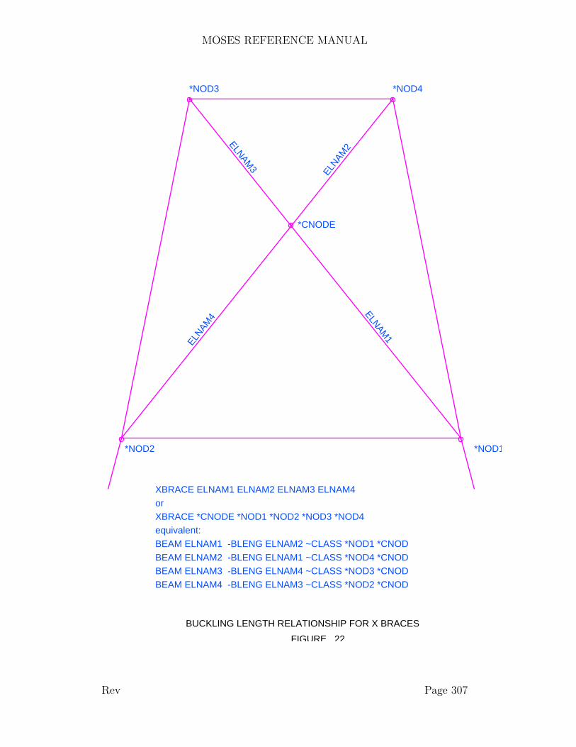
MOSES REFERENCE MANUAL
BUCKLING LENGTH RELATIONSHIP FOR X BRACES
FIGURE 22
*CNODE
*NOD3 *NOD4
*NOD1*NOD2
ELNAM3
ELNAM
2
ELNAM
4ELNAM
1
XBRACE ELNAM1 ELNAM2 ELNAM3 ELNAM4orXBRACE *CNODE *NOD1 *NOD2 *NOD3 *NOD4equivalent:BEAM ELNAM1 -BLENG ELNAM2 ~CLASS *NOD1 *CNODBEAM ELNAM2 -BLENG ELNAM1 ~CLASS *NOD4 *CNODBEAM ELNAM3 -BLENG ELNAM4 ~CLASS *NOD3 *CNODBEAM ELNAM4 -BLENG ELNAM3 ~CLASS *NOD2 *CNOD
Rev Page 307
MOSES REFERENCE MANUAL
XIII. CONNECTIONS AND RESTRAINTS
In MOSES, bodies are connected together or to ground with special elements calledconnectors or restraints. A restraint is an element which acts like a connector duringa stress analysis, but does not act during a simulation. Basically, restraints are oflimited use. Connectors, however, are quite important. In general, there are threecategories of connector: flexible, rigid, and connector assemblies. Flexible and rigidconnectors connect a body to either another body or to ground. Connector assembliesare sets of simple connectors which act in unison and may connect more than twobodies. Rigid and flexible connectors actually serve the same purpose – they createa force between two points. The real difference is how the force is computed. Withflexible connectors, the force is computed based on a force–deflection rule and thegeometry of the system. Rigid connectors yield constraints on the motion of thebodies. Excepting numerics, a very stiff flexible connection and a rigid connectionshould yield the same result. In reality, when the stiffness gets substantial, numericalprecision is lost and the solutions are either difficult or impossible to obtain. In thesecases, rigid connections can ameliorate the difficulties.
Here, we will call connectors ”simple” if they are not assemblies. All simple connectorsare defined with the following command in the MEDIT menu:
CONNECTOR, CNAME, –OPTIONS, ∼CLASS, *NODE(1), *NODE(2)
and the available options are:
–GOi, X, Y, Z–ANCHOR, THET, DTA–EULER, E DATA–NUM APPLIED, NUMBER–TUG, ANG, DIST
and restraints are defined with
REST, ∼CLASS, *NODE(1), *NODE(2)
Here, ∼CLASS is a previously defined class and *NODE(1), and optionally *NODE(2),are the nodes to which the connector will be attached. The details of the options andthe number of nodes required depends on the category of connector class. The –GOioptions are used to define offsets at the ”ith” vertex of the element. Here, –GO1defines offsets at the first end, etc. The values X, Y, and Z define the coordinates ofthe offset (inches or mm) and are defined in the part system. If only –GO is specified,then all vertices will have the same offsets. In all cases, an offset is defined as thevector from the node to the vertex of the member. To connect a body to ground,
Rev Page 308
MOSES REFERENCE MANUAL
either the second node should be omitted, or it should be a fixed node. Fixed nodesare nodes which belong to a special part GROUND.
The –ANCHOR option is applicable only to connectors which have a class type ofROD or B CAT, and must be used to define the location of the ground attachmentfor these classes. Here, the location is defined relative to *NODE(1) by a headingand a distance. THET is the heading (deg.) from the vessel X axis, (in the currentconfiguration, positive toward Y) to the anchor line, and DTA is the horizontaldistance (feet or meters) from the attachment point to the anchor. The verticalcoordinate is not defined since it is given by the depth of the anchor on the classdefinition.
The –EULER option is applicable only to connectors which have a class type ofGSPR, LMU, or FOUNDATION and it is used to change the element system ofthe connector. By default, the element system is aligned with the body system of thebody to which the first node belongs. E DATA can be a set of Euler angles whichchanges this orientation. There are three angles: a roll, a pitch, and a yaw. These arerotations about the element system. In particular, suppose that the element systemis in its default position. Now, give it a yaw (a rotation about the element Z axis),and then a pitch (a rotation about the new element Y axis), and finally a roll (arotation about the new element X axis) to put it into the desired position. As aquick way of defining these angles, MOSES will also accept values of +X, –X, +Y,–Y, +Z, or –Z. These align the element X axis with the body axis specified. In otherwords, a value of –Y is the same thing as an value of 0, 0, –90.
The option –NUM APPLIED allows one to have a multiplier, NUMBER, for aconnector. The results for a connector are first computed based on the specifiedproperties, and then all results are multiplied by NUMBER. In particular, the damp-ing, stiffness, mass, matrices and the force are multiplied. This option works onlywith flexible connectors.
The final option is applicable only to –TUG connectors. Here, ANGLE is the globaldirection of the tug, positive when measured from the global X axis towards theglobal Y axis. DIST is the distance (feet or meters) from the attachment point on abody, *PT, to the tug.
The string function:
&CONNECTOR(:CON SELE, –OPTION)
returns the current data for each connector selected by the selector :CON SELE. Thefirst token is the name of the connector and the remainder depends upon the options.
Rev Page 309
MOSES REFERENCE MANUAL
For a type of
• –TENSION the remainder is by the magnitude of the force in the connector,• –HORIZONTAL the remainder is the magnitude of the X and Y components
of the force,• –FORCE the remainder is the X, Y, and Z components of the force in the
connector,• –RATIO the remainder is the ratio of the acting force in the connector to the
breaking strength,• –E NAMES the remainder is the names of the points at the ”ends” of the
connector,• –E COORDINATES the remainder is the coordinates of the ends of the
connector in the body system of the body,• –ANCHOR the remainder is the three coordinates of the anchor,• –LENGTH the remainder is the current length of the first segment of the
connector,• –HEADING the remainder is the local body heading of the connector,• –G HEADING the remainder is global heading of the connector,• –FRICTION the remainder is the friction in the connector,• –T MULT the remainder is the current trust multiplier for the connector,• –T ANGLE the remainder is the current body angle of the thrust of the
connector,• –R ANGLE the remainder is the current angle of the rudder for the connector,• –HP ANCHOR the remainder is the horizontal pull on the anchor for the
connector,• –VP ANCHOR the remainder is the vertical pull on the anchor for the con-
nector, and• –L ON BOTTOM the remainder is the line on bottom for the connector.
Since there are many different situations that MOSES can analyze there is a commandthat allows one to change many of the properties of connectors as different situationsarise. This command is discussed in the section on altering connectors.
Rev Page 310

MOSES REFERENCE MANUAL
XIII.A Defining a Pulley Assembly
A pulley assembly is simply a set of connectors connected with pulleys. Such anassembly is defined by the command
ASSEMBLY PULLEY, PUL NAME, EL(1), ........, EL(i)
Here, PUL NAME is the name you wish to give to the pulley assembly, and EL(i)are previously defined connector element names. The connector elements must beeither H CAT (without the exact option) or B CAT elements. If one has a B CATelement, then it must be the last element of the assembly. In essence, a ASSEMBLYPULLEY assembly is a single line which passes through n–1 pulleys. If all of theelements are H CATs, then the computation is exact, and all of the properties ofeach segment of each connector are properly accounted for. If, however, one has anassembly with a B CAT element, then the idealization is exact only when the sizeof the wire for the H CAT element is the same as the top segment of the B CAT.Here, also, any additional springs on the H CAT element will be ignored. Theseelements can be used in any way that H CAT or B CAT connector can be used. Inparticular, the &CONNECTOR command can be used to change the length of thefirst segment or the change the activity of the element.
Rev Page 311

MOSES REFERENCE MANUAL
XIII.B Defining a Launchway Assembly
A launchway is a complicated set of connections which are collectively referencedwithin MOSES by the name &LWAY. The launchway is composed of at least twolaunch legs each one of which is defined via the command:
ASSEMBLY LLEG, *J(1),*J(2), .. *J(n), BODY NAME(1), XB, YB, ZB,:B1(1), .. \
:B1(n) BODY NAME(2) :B2(1), ..... :B2(n), –OPTIONS
and the available options are:
–FRIC, DYNFRC–TPIN, TPRIDEP, XP, YP, ZP, MAX ANGLE, TSECDEP, DIST–BEAM, LENP, EIP, LENS, EIS
Here, *J(1), ... *J(n) are the node names of the nodes along the launch cradle ofthe jacket, in order, where *J(1) is the first node which will enter the water and*J(n) is the last node which will enter the water. The launch cradle is consideredthe part of the jacket that rests on the barge skidway. An illustration of the nodearrangement is shown in Figure 23. BODY NAME(1) is the body name assigned tothe barge where the tiltpins are attached, and XB, YB, and ZB are the coordinates,in the BODY NAME(1) body system, of the beginning of the skidway on bodyBODY NAME(1). Here, the skidway should be considered to be at the height ofthe jacket launch leg centerline above the barge origin. Also, :B1(i) are selectorsfor the nodes in BODY NAME(1) which will be used for connecting the jacket tothe barge. BODY NAME(2) is the name of an optional second body over which theskidway may pass, and :B2(i) are again node selectors.
The dynamic coefficient of friction for the launchway is specified with the –FRICoption as DYNFRC. The tiltbeam geometry for the launchway is specified via the–TPIN option. Here, XP, YP, and ZP are the body coordinates of the primarytiltpin (feet or meters), TPRIDEP is the height of the primary tiltbeam (feet ormeters), MAX ANGLE, the maximum angle the tiltbeam is allowed to rotate untilthe secondary tiltbeam becomes active (deg.), TSECDEP, is the height of the sec-ondary tiltbeam (feet or meters), and DIST is the distance along the skidway fromthe primary tiltbeam to the secondary one (feet or meters). Here again, the depthof the beams should be considered to be the vertical distance from the tiltpin to thecenterline of the jacket leg. If there is no secondary tiltbeam, one should omit thevalues for MAX ANGLE, TSECDEP, and DIST. An illustration of the tiltbeam isshown in Figure 24.
The stiffness of a tiltbeam is input using the –BEAM option. Here, LENP is the
Rev Page 312
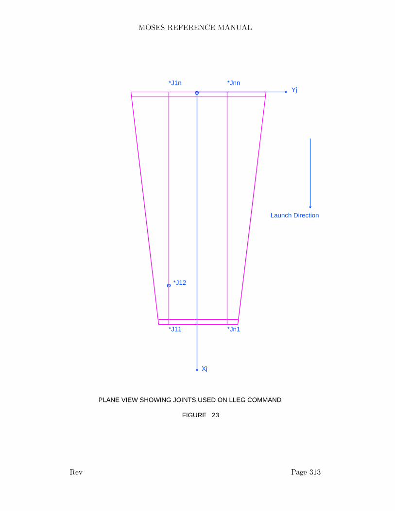
MOSES REFERENCE MANUAL
PLANE VIEW SHOWING JOINTS USED ON LLEG COMMAND
FIGURE 23
Yj
Xj
Launch Direction
*Jn1
*Jnn
*J11
*J12
*J1n
Rev Page 313

MOSES REFERENCE MANUAL
DIST
TS
EC
DE
PT
PR
IDE
P
Xp, Yp, Zp
X Axis
Z A
xis
XB, YB, ZB
TILTBEAM GEOMETRY
FIGURE 24
length of the primary tiltbeam (feet or meters), and EIP is the stiffness (bforce–ft**2 or bforce–meters**2). LENS and EIS are the length and stiffness values forthe secondary tiltbeam, respectively. If there is no secondary tiltbeam, these valuesshould be omitted.
The order of input of the ASSEMBLY LLEG commands is important as it is usedto establish the launch coordinate system of the jacket. The axes of this coordinatesystem are set as follows: The X axis is parallel to a line connecting *J(1) and *J(n),and is directed towards *J(1). The jacket is launched in the positive X direction.The origin of this system is midway between the trailing joints given on the first andlast ASSEMBLY LLEG commands, and the Y axis is along the line connectingthe *J(n) on the last ASSEMBLY LLEG input with *J(n) on the first one input.The Z axis is determined from the right hand rule.
At the conclusion of the MEDIT Menu, the orientation of the body systems will,in general, change. MOSES will change the body system of the jacket as describedabove. It will also change the orientation of the barges so that their body X axis willbe aligned with that of the jacket. In contrast to the jacket, there is no translationof the barges’ body system.
Rev Page 314
MOSES REFERENCE MANUAL
XIII.C Defining a Sling Assembly
A sling assembly is an abstraction of the lines which a lift vessel can apply to anotherbody. Here, the point at the boom where the connection begins is called the boompoint. This point is connected to the hook by a length of line, and in turn the hook isconnected to several points on the body by other lines. In MOSES, the hook can beconnected to the body with up to four elements. This set of lines is called a tip–hookset, and is referred to by a name given to the hook. Several different tip–hook setscan be defined connecting different bodies.
Each tip–hook set is defined by a command:
ASSEMBLY T–H DEFINITION, NAME, BHE, EL(1), ........, EL(4),–OPTIONS
and the available options are:
–INITIAL,–ORIENT,–VERTICAL–DEACTIVATE
Here, NAME is the name you wish to give the tip–hook set, BHE is the name ofthe element connecting the boom point to the hook, and EL(i) are the names ofthe elements connecting the hook to a body. All of these elements must have beenpreviously defined with CONNECTOR commands, must have a class category ofSLING, and must have a single node. Additionally, all of the nodes of the EL(i)must belong to the same body.
The –INITIAL option instructs MOSES to ”initialize” the set. If this option isspecified and this is the first tip–hook set defined, the body will be moved so thatthe hook point is directly below the boom point. If the option is selected and this isnot the first tip–hook set, then the length of the tip–hook elements will be changedso that there is no sag in the lines.
The –DEACTIVATE option instructs MOSES to to deactivate all previously de-fined tip–hook sets.
The –ORIENT option can be used to alter the definition of the body system ofthe body to which the EL(i) are connected. With this option, the order of the slingnodes is used to define the local body system. The origin of this system is definedas the midpoint of the vector connecting the first two sling nodes. The local Y axisis in the direction of the first node toward the second, the local Z axis is from the
Rev Page 315

MOSES REFERENCE MANUAL
second node to the third, and the local X axis is given by the right hand rule.
During static processing, the configuration of the body is defined by the height of thehook attachment point above the waterplane and two angles. These two angles arecalled pitch and roll. The two angles are defined by vectors which can be defined viaa &DEFAULT command. The –VERTICAL option can be used to automaticallydefine these three quantities. Here, pitch is the angle which the normal to the planeformed by the sling nodes makes with the waterplane, roll is the rotation of the linedefined by the first two sling nodes, and height is measured to the midpoint of theline connecting the first two nodes.
Once the sling is defined, the lengths of the tip–hook elements can be changed with&INSTATE –SL SET. MOSES will place the system in the specified configurationand compute the lengths of each tip–hook element so that there is no slack in theassembly. Also, the &CONNECTOR command can be used to change the lengthof the boom element and deactivate the tip–hook set. The name to use here is the,NAME, the name given the set.
Rev Page 316
MOSES REFERENCE MANUAL
XIII.D Defining a Pipe or Riser Assembly
A pipe assembly is a ROD element along with a set of elements which connectthe ROD to a set of bodies. The connecting elements can be either DAVIT orROLLER elements. Here, DAVIT elements are lines which connect the pipe, whileROLLERs are one–sided constraints which keep the ROD on a pipe–lay route. Suchan assembly is defined by the command
PIPE, ∼PIPE CLASS, EL(1), ........, EL(i), –OPTIONS
and the available options are:
–PIPE TENSION, TLOWER, TUPPER
Here, ∼PIPE CLASS is the name of a ROD class which will be used to define theproperties of the pipe, and EL(i) are the connector element names of elements whichhave been previously defined. The connector elements must be either DAVIT orROLLER elements, and these types of elements cannot be mixed. MOSES assumesthat pipe is laid in the negative X global direction, so that all of the connectors mustlie along the global X axis when the assembly is defined. The pipe itself is given aname &PIPE and the assembly has a name of &PIPE/ASSEMBLY.
The use of the –PIPE TENSION option depends on the type of connection. For anassembly of ROLLER elements, TLOWER defines the smallest allowable tensionervalue (bforce) and TUPPER the largest allowable tension (bforce). With a ROLLERassembly, the last roller defined is the tensioner. With a DAVIT assembly, the valueof TLOWER (bforce) is the nominal initial tension in the pipe where it connects tothe first davit, and TUPPER is not used.
A special situation occurs when one has only a single roller. In this case, MOSES willtreat the pipe assembly as a vertical pipe with a tensioner, so that one can simulatea riser. Here, the bottom of the rod is placed directly below the roller connection sothat the pipe will have a tension of TUPPER.
When initializing a pipe assembly other than a vertical one, it is assumed that thepipe behaves as a catenary. (Thus, the use of the word nominal as regards the initialtension.) MOSES uses this assumption as initial estimates for the configuration of theassembly, and then iterates a solution to the nonlinear problem. A stinger is initiallytensioned so that either the slope of the pipe matches the slope of the last two rollers,or all of the pipe is off of the bottom. The assembly problem is particularly difficultwith davits. Here, the assembly is initialized by using only the length of the firstdavit and the nominal pipe tension. The lengths of the other davit lines are then
Rev Page 317

MOSES REFERENCE MANUAL
computed to conform to this estimate.
Rev Page 318

MOSES REFERENCE MANUAL
XIII.E Defining a Control Assembly
A control assembly is simply a set of connectors connected to a control. Such anassembly is defined by the command
ASSEMBLY CONTROL, CONTROL NAME, PE(1), ........, PE(i) –OPTIONS
Here, CONTROL NAME is the name you wish to give to the control assembly, andPE(i) are previously defined PROPULSION connector element names.
Here the options are either
–SENSORS SG(1), SEN(1), .... SG(n), SEN(n)
Simply, the control system will compute an x and y force and a yaw moment givenby:
F(i) = sum [ SG(k) SR(k,i) ]
Here SG(k) are the multipliers defined with the –SENSORS option and SR(k,i) isthe ”sensor reading” for the kth sensor. The i is the degree of freedom for the sensor.The thrust is allocated amount the thrusters based on a least squares fit.
Normally, the sensors are ”VECTOR” sensors where the first point of the vector isa point on the body and the second point is a point on ground. The signal is thevector between the two points which we want to be zero.
Propulsion units with rudders are treated differently. They can control only yaw andthe thrust is not altered by the control system. In other words, one sets the thrustwith a &CONNECTOR xxx –SET PROPULSION command and the control sys-tem will control the rudder to achieve a given heading.
Rev Page 319
MOSES REFERENCE MANUAL
XIII.F Defining a Winch Assembly
A winch assembly is simply a set of connectors connected to a winch. Such anassembly is defined by the command
ASSEMBLY WINCH, WINCH NAME, EL(1), ........, EL(i) –OPTIONS
Here, WINCH NAME is the name you wish to give to the winch assembly, andEL(i) are previously defined connector element names. The connector elements mustbe either B CAT, H CAT, SL ELEM, ROD, GSPR, LMU elements, or theSLING element connecting the boom to the hook on a tip–hook assembly.
Here the available option is
–WINCH FULL WEIGHT, MAX TORQUE, S MOMENT, D MOMENT, \TOT LENGTH, FULL GYRADIUS, FULL RADIUS
This option is used to define the mechanical properties of the winch and alterna-tively the second defines the velocity of the winch as a function of time. Here,FULL WEIGHT is the weight (feet or meters) of the drum plus the wire.The nextthree values define either the maximum applied torque, MAX TORQUE, maximumapplied torque or two moments applied by a brake. S MOMENT is the static mo-ment due to the brake and D MOMENT is a factor which when multiplied by thesquare of the angular velocity is the dynamic moment due to the brake All three ofthese are in bforce–blength. The last three values are: the total length of wire onthe drum, the radius of gyration of the drum plus wire when full, and the radius ofgyration of the drum plus the wire when the winch is full in feet or meters.
Rev Page 320

MOSES REFERENCE MANUAL
XIII.G Altering Connectors
So that many different situations can be analyzed, MOSES provides the ability topartially alter the definition of the connector system. This is performed with onecommand, &CONNECTOR, which has several options, most being applicable toa particular class of connector. The form of this command is:
&CONNECTOR, :CONN SEL(1,1), ..., :CONN SEL(n,1), –OPTION(1), \:CONN SEL(1,2), ..., :CONN SEL(n,2), –OPTION(2), \:CONN SEL(1,m), ..., :CONN SEL(n,m), –OPTION(m)
where the options applicable to all connectors are:
–INACTIVE–ACTIVE
which makes a set of connectors inactive or active. Each option operates on the list ofconnectors immediately preceding it. The first option defines the connectors whosenames are selected by the selectors :CONN SEL(i) to be inactive. Inactive connectorscan be reactivated by simply issuing the second option.
For connectors with types of ROD, SL ELEM, B CAT, and H CAT more thingscan be accomplished with &CONNECTOR. To alter the length of the first segmentof a line, use the options:
–LENGTH, LEN–L DELTA, DLEN–L HORIZONTAL, FORCE–L TENSION, FORCE
Here, :CONN SEL(i,j) are the selectors for lines whose length will be altered, andthe method of specifying the new length is controlled by the options. If one uses–LENGTH, he is simply defining each line which matches the selectors to have alength of the first segment of LEN (feet or meters). Using –L DELTA is similarto the above except that DLEN (feet or meters) is added to the existing length.Alternately, one could specify either –L HORIZONTAL or –L TENSION. Withthese options, a new length of the first segment will again be defined, but here, thenew length is calculated so that either the tension or horizontal force has the valueFORCE in the initial configuration.
To alter the location of the anchor, use the options:
–ANCHOR, XA, YA, ZA–A HORIZONTAL, FORCE
Rev Page 321
MOSES REFERENCE MANUAL
–A TENSION, FORCE
Here, :CONN SEL(i,j) are the selectors for lines whose anchor location will be al-tered, and the method of specifying the new location of the anchor is controlled bythe options. If one uses –ANCHOR, he is simply defining the global x, y and zcoordinates (feet or meters) of the anchor of each line which matches the selectors.The z coordinate specified here is honored for all flexible connectors except a type ofH CAT, where it is ignored. Alternately, one could specify either –A TENSION or–A HORIZONTAL which instructs MOSES to compute the location so that eitherthe tension or horizontal force has the value FORCE in the initial configuration.
The force of H CAT connectors is computed with the aid of a ”lookup table”. Theforce properties of the line are computed as a function of distance from the anchorand stored in a table when the connector is defined or its properties changed. Now,this table produced quite accurate results for changes in horizontal directions, butthe changes due to vertical motion are approximated. If one is interested in movinga body vertically, he may need to recompute the table as the body moves. The Theoption
–G TABLE}
will force MOSES to recompute the table at the current position.
For ROD connectors, three additional things can be altered with the &CON-NECTOR command with the options:
–A STIFF, STADGX, STADGY, STADGZ–TOP MOMENT, YES/NO–ST ADDITION, INONUM, STADGX, STADGY, STADGZ–ZERO BSTIF, YES/NO
Normally, the top of the rod is ”pin” connected to the body, and a default stiffnessis assigned for the connection at the first node (the ”anchor”). The default dependson the type of rod: if it is a ”straight rod” a large stiffness is used, while for a”mooring line” type of rod a much smaller stiffness is defined. The option –A STIFFallows one to redefine the anchor stiffness. Here, STADGX, STADGY, and STADGZare the global X, Y, and Z values of the stiffness in bforce/blength. If one uses –A STIFF 0 0 0, then the rod will have no restraint at the anchor. Similarly, the–TOP MOMENT option changes the connection behavior at the top. If it is usedwith a YES/NO of YES, then the top connection will apply a moment; otherwise, itwill apply only forces. The –ZERO BSTIF option changes the connection behaviorat the bottom. If it is used with a YES/NO of YES, then the stiffness at the bottom
Rev Page 322

MOSES REFERENCE MANUAL
will be applied, otherwise the bottom will be free to move.
The option –ST ADDITION allows one to add a diagonal stiffness matrix at inter-mediate points along the rod. Here, INONUM is the intermediate node number wherethe stiffness will be added. These nodes are numbered with the bottom being 1, sothat to add a stiffness one node above the bottom, it should be added with INONUMequal 2. STADGX, STADGY, and STADGZ are the same as for –A STIFF.
One may alter the settings of a propulsion connector with: with the option:
–SET PROPULSION, T MULT, T ANGLE, R ANGLE
of the &CONNECTOR command. Here, T MULT is the fraction of the maximumthrust ( –1 <= T MULT <= 1) which will be applied, T ANGLE is the angle thatthe thrust will be applied, and R ANGLE is the angle of the rudder. Both of theseangles should be –90 <= ANGLE <= 90.
One may alter a tug connector with: with the options:
–T FORCE, FORCE–T LOCATION, ANG, DIST–T DYNAMIC, PERCENT FORCE, PHASE
of the &CONNECTOR command. The values for FORCE, ANG, DIST, PER-CENT FORCE and PHASE have the same meaning as on the commands definingthe connector.
To define the special states of a foundation element for checking, one uses the option
–SET STATE, TYPE, MULT
of the &CONNECTOR command. Here, TYPE must be either PRELOAD orNOMINAL, and if TYPE is NOMINAL, then MULT is a multiplier which will beuse in computing the unity ratios otherwise it should be omitted. See the discussionin the section on Process Post–Processing of Connectors for details on the unity ratiocomputation.
A launchway assembly can be activated or deactivated by using the name &LWAYfor :CONN SEL(i,j). Also, one can alter some of the settings for the assembly oflaunchways with the options:
–LWA FRICT, DYNFRC
Rev Page 323
MOSES REFERENCE MANUAL
–LWA ANGLE, MAX ANGLE
Here, one selects the launchways which will have their properties altered with :CONN SEL(.).The –LWA FRICT option sets the dynamic coefficient of friction of the selectedrunners to DYNFRC, and the –LWA ANGLE option sets the maximum angle forthe first tiltbeam on the selected launchways to MAX ANGLE (degrees). The namesof the launchways are &LLEGi where i is a number assigned as the launchways weredefined.
Some things with pipe assemblies can also be changed with the &CONNECTORcommand. The options are:
–PIPE TENSION, TLOWER, TUPPER–DAV LENGTH, NEWLEN,–MOVE ROLLER, DX, DY, DZ,–LOC ROLLER, X, Y, Z,–A STIFF, STADGX, STADGY, STADGZ–TOP MOMENT, YES/NO–ST ADDITION, INONUM, STADGX, STADGY, STADGZ
Unless otherwise specified, :CONN SEL should be &PIPE. The –PIPE TENSIONoption sets the lower and upper bounds for the tensioner tension, TLOWER andTUPPER (bforce). The –DAV LENGTH option changes the length of the davitelements selected by :CONN SEL to be NEWLEN (feet or meters). If :DELEM se-lects the first davit element, then the entire assembly will be re–initialized and allof the lengths will be changed as when the assembly was defined. If the first ele-ment is not altered, then the selected lengths will be changed and a new equilibriumconfiguration of the pipe will be computed. The two options –MOVE ROLLERand –LOC ROLLER both result in the assembly being completely re–initialized.The first of these options moves rollers which match :CONN SEL from their cur-rent location by an amount DX, DY, and DZ (feet or meters). The second simplydefines the new location of the roller to be X, Y, and Z, (feet or meters), in thestinger body system. The last three options: –A STIFF, –ST ADDITION, and–TOP MOMENT operate on the pipe exactly as they do for a simple rod con-nector, and were discussed above.
Winch assembly properties can also be altered with the &CONNECTOR commandby using the option
–L DYNAMIC, ACTION, MULT, BOUND}
where :CONN SEL selects the winches to be altered. Here ACTION must be eitherMOTOR, BRAKE or the name of a CT LENGTH ”curve” that defines the
Rev Page 324

MOSES REFERENCE MANUAL
rate of change of length (feet or meters/sec) of the line. For the first of these, theMAX TORQUE will be multiplied by MULT and the winch motor will be turned onand the brake will be released. For the second, S MOMENT and D MOMENT willbut multiplied by MULT and winch motor will be turned off and the brake will beengaged. For the last action, the velocity curve will be multiplied by MULT. Here,BOUND is a bound on the line length. If MULT is greater than zero (letting outline) the BOUND is an upper bound on the line length. If MULT is less than zero(letting in line) the BOUND is an lower bound on the line length.
Normally control assemblies are changed only in the time domain. One can use the–SET PROPULSION option to set the values for statics, or use the option
–CONTROL
With this option, the control system will attempt to counteract the static mean wind,current, and wave forces.
Rev Page 325
MOSES REFERENCE MANUAL
XIV. PROCESSES
One thing which is fundamental to MOSES is the concept of a process. WheneverMOSES performs a simulation, the results are stored in the database by the processname. The name it uses is the ”current one”, or the last one which was referenced.To alter the ”current one”, one should issue the following command:
&DESCRIBE PROCESS, PRCNAM, –OPTIONS
and the only option is:
–EVENTS
When an &DESCRIBE PROCESS command is encountered, and the name forthe specified process is not already defined in the database, it will be added to thedatabase with the name specified. MOSES will then set the ”current” process to bethe one specified.
Here, by simulation results, we mean the initial and current configurations, the eventsfor the process, the activity status of the connections, the lengths of each mooring line,the load group multipliers, and the load set multipliers. In other words, all eventsof a simulation, the initial conditions, and any of the data defined by &COM-PARTMENT, &CMP BAL, &APPLY and &CONNECTOR commands isstored by process name. By altering the process name, one can actually consider sev-eral different connection situations using the same model. This is important, sinceone can also perform a structural analysis for several processes with the same factoredstiffness matrix.
Two types of data are stored by process name: constants and data which dependsupon event. Most of the data mentioned above are constants, and only one valuewill be associated with a process. The data which is stored by event is the configura-tion, the forces acting on the bodies, and any results of the &COMPARTMENT,&CMP BAL, &APPLY and &CONNECTOR commands. The constants arethe results of the &ENV command. Thus, a given process can have only a singleenvironment.
When the process name is altered, the new process will have all of the same settingsand initial condition as the situation immediately before the name was changed, butthe results of the previous simulations will appear to be ”lost”. They are, however, notreally lost. To recover them, one should issue another &DESCRIBE PROCESScommand to change the current process back to the name under which the results arestored. Thus, the process concept allows one to have many different sets of results
Rev Page 326

MOSES REFERENCE MANUAL
available for further processing.
If one wishes to have the events of the previous process available in the new one,he can specify the –EVENTS option when he created the process. Now, the newprocess is a true copy of the old process, and it can be altered as desired.
Most processes will have events defined by either a time domain simulation (theresults of a TDOM or LAUNCH command) or an upending sequence. At the con-clusion of a time domain or launch simulation, MOSES will revert to the situationat the beginning. Thus, issuing &STATUS after a time domain simulation willproduce the same result as issuing it before the simulation. In some cases, however,one may wish to construct a series of events which correspond to a set of equilib-rium configurations with different ballast conditions. This can be accomplished bycomputing an equilibrium configuration, and storing the results with a given eventnumber via the command:
&EVENT STORE, EVE NUMBER
The results of this ”simulation” can be post–processed as any other simulation inthe Process Post–Processing Menu. Notice, if this command is used when a processalready exists (a launch, time domain, upend, etc.) then it will corrupt the existingdata.
The string function which returns data for processes is:
&PROCESS(ACTION)
and ACTION must be either: PROCESS, C EVENT, MAX EVENT, or MIN EVENT.Which return the process name, the current event, the maximum event and the min-imum event for the current process.
Rev Page 327

MOSES REFERENCE MANUAL
XV. AUTOMATIC OFFSHORE INSTALLATION
Both the strength and weakness of MOSES is its flexibility; there is virtually nothingthat one cannot accomplish provided they are willing to spend the time. While theflexibility allows one to analyze everything, the price one pays is the cost of learning.If, however, one is willing to establish some rules and to decide on a fixed objectivefor a given analysis, then that analysis becomes routine.
A system of macros has been developed for the analyses of the installation of a jacket,deck, or other structure. In general, they can be used for loadout, transportation, lift,upend and launch. Considerable flexibility has been incorporated into this systemso that most cases can be easily considered. This system has been designed so thatseveral simulations that represent different phases of a structure can be performed,load cases generated, and one code check over all load cases can be produced.
With this system, one defines all of the data necessary for a transportation, launch,upend, lift or loadout analysis of a structure in a single data file with each analysisusing the same data. There are two general rules here to which one must adhere:
The dimension cannot be changed during the analysisOne must use a barge which conforms to conventions
By a barge conforming to conventions, we simply mean that all of the basic variableshave been set. A library of vessels is provided which conform. If one of these is notsuitable, you can prepare a model of your own. In preparing this model, you shoulduse the data file SAMPLE.DATA in the vessels library and which is discussed here.
To use this system, you should first read the documentation and then copy filesinstall.dat and install.cif from /ultra/hdesk/tools/install to your working directoryor by clicking here, and then modify them to suite your problem. Most of the workis involved with changing install.dat and we will discuss it first.
Most of the data required is defined in this file. The exceptions are the basic modeldata of the structures to be analyzed and the barge data. The structures data isassumed to be in other files which are inserted. The barge data is also inserted, butit is assumed to be in a special directory which contains all of the barge models.
Basic Data
The data required here is broken down into sections. The first section contains ”basic”
Rev Page 328

MOSES REFERENCE MANUAL
data required for any analysis and is basically self explanatory. The line
&DIMEN –SAVE –DIMEN METERS K–NTS
defines the units which will be used in the analysis. Two definitions are available tocontrol the pictures:
I SET DO MOVIE = .TRUE.
and
I SET RENDER = –RENDER GL
If the first of these is set .TRUE. then ”movies” of a launch and or upending willbe created provided you are rendering the pictures with GL. The second one definesthe rendering mode of the pictures. If –RENDER GL is set, then pictures will berendered with GL. To save time, you could use –RENDER WF. Finally, if you areusing a ”TERMINAL” interface, all pictures will be rendered as WF pictures and nomovies will be produced.
The following:
I SET WDEPTH = 390
defines the water depth. The ”margins”, or weight contingencies are defined by thetwo lines:
I SET MARGIN = 5I SET PER APPLY = 105
The first of these is for the basic steel in the model and the next is for any ”jointloads”.
The line
I SET T CODE = API WS
defines the type of code checks which will be computed. Here one can specify any codethat is accepted by the BEAM POST or JOINT POST commands. For transporta-tion, the macros will automatically build the proper load cases, but more informationis required:
Rev Page 329

MOSES REFERENCE MANUAL
I SET T CODE = API LRFD SO FACTOR SM FACTOR DM FACTOR
Here, the static internal forces and restraints are multiplied by SM FACTOR andcombined with DM FACTOR time the dynamic component before reporting or check-ing a code. Also, the static case times SO FACTOR is also checked. One should notuse an LRFD code for any other type of analysis.
The line
I SET CODE LIM = 1.33,1e6 1.,1.33 0.9,1.0 0.,0.9
defines the limits for the code check and joint check reports. If you do not changethis line, then the checks will be broken down ratios between 1. and 1.33, the nextfor ratios between .9 and 1, and the last for ratios between 0 and .9.
The elements for which code checks and/or fatigue will be performed are defined bythe following:
I SET C CODE = –SELECT @ –EXCEPT ∼dum@I SET N CODE = –SELECT @ –EXCEPTI SET N FAT = –SELECT @ –EXCEPT
Here, CLASS defines a variable that is used to determine the classes which will beconsidered for all three categories. If a class is not defined here, no element in thisclass will be considered for Beam Check, Joint Check, or Joint Fatigue. N CODE isa variable which defines the joints which will be considered. If a joint is not selected,no results for Joint Check or Joint Crushing will be produced for this joint. Finally,N FAT defines the joint to be considered for Joint fatigue.
Fatigue Data
If one wants to consider fatigue, then he must define several things. One thing, whichis essential, is that the duration data which will be used must be specified. This iswith an option of the transportation macro and is discussed below. Also, one maywish to alter one or more of the following:
I SET FAT LIM = 1.,1.e6 0.25,1 0,0.25I SET SCF = EfthymiouI SET SN = XPI SET B SN = AWSE
The first of these defines the limits for which the fatigue reports will be broken down.If this is not changed, one will receive 3 reports for joint and beam fatigue: The first
Rev Page 330

MOSES REFERENCE MANUAL
will have CDRs above 1, the second will have CDRs between .25 and 1, and the lastwill have CDRs between 0 and .25. The next two lines deal with tubular joint fatigue.Here, SCF defines the type of SCFs which will be computed during fatigue. The SNvariable defines the SN curve for Joint Fatigue. In either of the variables, multiplecurves can be used. For example,
I SET SN = XP X
will produce fatigue results for both the XP and the X curves. The B SN variabledefines the SN curve which will be used for Beam Fatigue, and the &REP SELECTcommand defines a new type of SN curve, AWSE. Here, the default SCFs for beamwhich are not tubes are set to 1, and the AWSE curve is used for beam fatigue.
Report Data
The following command defines the cover page for the report. Be sure to enclose thevariables in single quotes(’) if they are more than one word.
I BEGIN,–OPTIONS
And the available options are:
–TLINE1, ’XYZ EXPLORATION and PRODUCTION’–TLINE2, ’8 Pile Jacket for the COWABUNGA Field’–TLINE3, ’Installed Offshore Timbuktu’–CLIENT, ’QRS Engineering, Inc’–FOOTER, ’8 Leg Jacket’
Barge Data
This data is necessary only for a launch or transportation.
USE VES BARGE
The data for the barge being used is more restrictive than that for the structure.Again, guidance on how to make your own barge model can be found here. Thereason for this is that the barge tilt beam data and many other things are necessary.Thus, the barge used must be one of the barges supplied, or a new barge defined inthe same format. Here, BARGE, should be the name of the barge one wishes to use.
Structure Data
This section of data needs to be completed for any analysis. Here, one is calling a
Rev Page 331
MOSES REFERENCE MANUAL
macro which sets up the data required for each structure to be analyzed. The syntaxof the macro is:
MODEL IN NAME FILE X Y Z –OPTIONS
And the available options are:
–PORT NODES, *P1, *P2, *P3 ...–STBD NODES, *S1, *S2, *S3 ...–ORIENT, *O1, *O2, *O3–TOP NODE, *TOP NODE–EXTREMES, P NAM(1), *P NODE(1), P NAM(2), *P NODE(2) ...
The variable ”FILE” defines the file which contains the model for the structure.
Even thou the –PORT NODES and –STBD NODES are listed as options they arenecessary. If you have a transportation analysis with multiple structures, you shouldhave a ”MODEL IN” for each structure. Sometimes you may have a jacket anddeck on the same barge, or two deck sections on the same barge. The MODEL INcommand can also be used to input files that describe miscellaneous cargo, such aspiles or boat landings. In this case, FILE for each cargo would contain the appropriatecommands to adequately describe the cargo, such as PGEN and #WEIGHT.
The variable ”NAME” defines the type of structure. Any name up to eight charactersmay be used, but the names JACKET and TRIPOD are special. Also, for multiplestructures on one barge, the first three characters of the name must be unique. Thisdefinition controls the type of connections which are established for transportationand the initial setup for upending. For upending with a type of TRIPOD, the axessystem will not be moved when slings are added.
The variables X, Y and Z define the location of the ”origin” of the structure on thebarge. Here, X is the location aft of the bow, Y the distance off of the centerlineand Z is the height above the barge deck. The meaning of origin changes withhow the structure is oriented. Normally, the two options –PORT NODES and–STBD NODES define the orientation. If they orient the body, the origin is themidpoint of the trailing port and starboard nodes. If the –ORIENT option is used,the origin is the first node specified.
The two options –PORT NODES and –STBD NODES are used to define thenames of the nodes on the ”launch legs”. The first node for each variable is the nodeat the leading edge of the jacket and the last is the node at the trailing edge of thejacket. The leading edge is defined as the end of the jacket that enters the waterfirst. The PORT NODES are on the port side of the barge while the STBD NODES
Rev Page 332

MOSES REFERENCE MANUAL
are on the starboard side. When specified, these nodes define the orientation of thestructure on the barge. They are also used to define barge/structure connections ifa V LWAY connection is specified or if one performs a loadout analysis.
For a structure which is not symmetrical about the barge centerline the orientationscheme is different. Here, the –ORIENT option is used. This option defines threenodes. The first node is where distances for positioning will be measured and isnormally at the bottom of the leg that is parallel with the deck edge, assuming thetop of jacket faces aft. The second node is along the leg from the first node, and thethird node is on the other side of the barge, usually along the horizontal level in linewith the first node. Y is the distance from the centerline of the barge to the firstnode, positive towards starboard. Note that if one specifies starboard nodes and anegative Y then the jacket will be placed under the barge.
–TOP NODE option is used for an initial guess during upending and stabilitysprings for other types of analysis. This node should be on the face of the structurewhich is the highest above the water in the initial floating position and should notbe attached to any slings.
Points used for reporting purposes can be specified with the –EXTREMES option.Here, a point name and node name is required for each point of interest. For a jacket,these are normally the top and bottom nodes of each corner leg.
For deep water fixed leg structures, the inside diameter of leg compartments canvary substantially. For these situations, there is a useful command for defining veryaccurate tank definitions, which has the following syntax:
I TANK TANK NAM, *BOT NOD, *TOP NOD, E BOT, E TOP, –OPTIONS
And the available options are:
–F VALVE, VF DIA, VF DIST–V VALVE, VV DIA, VV DIST–ELEVATION–PERMEABILITY, PERM–B NODES, BN(1), BN(2), ....
Here, TANK NAM is the name given to the tank, and *BOT NOD and *TOP NODare the names of the bottom and top nodes on the jacket leg where the tank resides.The variables E BOT and E TOP provide the locations of the bottom and top of thetank, respectively. These are the bulkhead locations inside the leg. If this informationis not supplied, the bulkhead locations will be assumed to be at the bottom andtop nodes. If the –ELEVATION option is used, these bulkhead locations will be
Rev Page 333
MOSES REFERENCE MANUAL
assumed to be jacket elevations, where the jacket origin is at the inplace waterline,and Z is vertical up. Without this option, the bulkhead locations are assumed tobe the length along the leg from the bottom node. Bulkhead locations are specifiedin feet or meters, depending on the current units. The diameter and location of theflood and vent valves are specified with the –F VALVE and –V VALVE options.For this information, valve diameter is specified in inches or millimeters, and thevalve location is specified in feet or meters. The valve locations here are according tothe use of –ELEVATION. If no valve information is provided, a 4 inch flood valvewill be located at the bottom node, while a 4 inch vent valve will be placed at the topnode. The –PERMEABILITY option allows one to specify the permeability forthe tank. Normally legs which contain tanks are straight. The –B NODES optionallows one to specify joints at which the leg has a break in slope. The I TANKcommand will use the jacket model to prepare the proper TUBTANK definitions,capturing all the changes to inside diameter along the elements defining a jacket leg,including changes to segments in the elements.
Connector Data
There are three different categories of connectors that can be defined for use ina simulation: SLINGS, TIEDOWN CONNECTORS and VERTICAL SUPPORTS.Each of these categories uses the I CONNECTOR command, followed by a typedescription and then the required data.
To define an upending sling assembly for use in a jacket upending analysis, a type ofUP SLING is used, and has the following syntax:
I CONNECTOR UP SLING *U1 L1 *U2 L2 ...
The data that follows the connector type is a set of node names and harness lengthsin feet or meters. The number of pairs defined gives the number of sling elementswhich will be attached. For a body name of JACKET, the order of the nodes is usedto define the local body system. The origin of this system is the midpoint of thevector connecting the first two sling nodes. The local Y axis is in the direction of thefirst node toward the second, the local Z axis is from the second node to the thirdand the local X axis is given by the right hand rule.
To perform a lift analysis, you will need a connector type of LIFT SLING:
I CONNECTOR LIFT SLING *L1 LEN1 *L2 LEN2 *L3 LEN3 *L4 LEN4
A sling will be constructed from each of the nodes specified to the common hook
Rev Page 334

MOSES REFERENCE MANUAL
point.
Tiedown connectors for a transportation analysis can be defined using the followingI CONNECTOR types:
I CONNECTOR 4 TIE ∼TD CLASS *TIE1 *TIE2 ...I CONNECTOR V BRACE ∼TD CLASS *TIE1 *TIE2 ...I CONNECTOR P BRACE ∼TD CLASS *TIE1 *TIE2 ...I CONNECTOR H BRACE ∼TD CLASS *TIE1 *TIE2 ...I CONNECTOR PCONNECT TIEDOWN DATA
I CONNECTOR XY DELTA ∼TD CLASS DELTA X DELTA Y *TIE1*TIE2 ...
When the 4 TIE connector type is specified, 4 tiedowns with the properties of∼TD CLASS will be generated at each node specified. The ∼TD CLASS must bedefined before it is referenced on the I CONNECTOR 4 TIE command. Thetiedowns will be arranged in star pattern, with each tiedown 45 degrees from a lon-gitudinal axis that passes through the tiedown node and is parallel to the bargecenterline. The longitudinal and transverse distance from the referenced structurenode to the deck end of the tiedown is the same as the vertical distance of the refer-enced node above the barge deck.
Connectors types of V BRACE, P BRACE and H BRACE are all very similarto one another. The names here refer to Vertical Brace, Pitch Brace, and HorizontalBrace, respectively. The V BRACE takes only dynamic vertical load, no grav-ity load, and creates an element from the referenced node to the barge deck. TheP BRACE takes only longitudinal dynamic load, and creates a horizontal elementthat is 5 feet or meters long. The H BRACE takes only transverse dynamic load,and creates a horizontal element from the referenced node to the side shell. As withthe 4 TIE type, the referenced ∼TD CLASS must have been previously defined.For all these tiedown types, the connection at the barge end of the tiedown takes nomoments, meaning a pinned connection.
If none of the above tiedown connector types are suitable, one can still define connec-tors explicitly, and place this definition in this file. For tiedowns, this is done withthe ICONNECTOR PCONNECT command. While this format allows for anyvalid PCONNECT data, the following information is normally provided:
I CONNECTOR PCONNECT DX DY DZ ∼TD CLASS *NOD *B@
For structure descriptions that include tiedowns, the tiedowns should be removedfrom the structure file and placed in this file using the above I CONNECTOR
Rev Page 335
MOSES REFERENCE MANUAL
PCONNECT method.
The I CONNECTOR XY DELTA command provides an easy way to definetiedowns where the barge end remains at the same height as the referenced nodeon the structure. DELTA X and DELTA Y refer to the distance from the referencednode to the barge end of the tiedown.
Vertical supports that take gravity load can be defined with these I CONNECTORtypes:
I CONNECTOR V LWAYI CONNECTOR V CAN ∼CAN CLASS *C1 *C2 ... –OPTIONI CONNECTOR V REST ∼REST CLASS *R1 *R2 ...
The V LWAY type will create a vertical connector using the node names providedon the –PORT NODES and –STBD NODES options of MODEL IN. This willactually create a structural element that simulates the launchway on a barge, usingthe launchway information provided in the barge model. If this launchway informa-tion is not available, a WBOX beam is generated that is 48 inches deep, 48 incheswide, with 1 inch plates for the flanges and sides, and 2 inch plate for the centerplate. The connections created here are gap elements. For spectral load cases, onlya linear structural solution can be performed, so the gap elements have no effect onthese cases. For time domain load cases, a nonlinear structural solution is performed,which involves iteration over the support nodes to release those supports that showtension.
The connector type V CAN provides a vertical support can with the properties pro-vided by the can class ∼CAN CLASS. A beam element is created from the referencednode to the barge deck, with moments about the local Y and Z axes released at bargeend. If one specifies the option –DO HORIZONTAL, then restraints will be addedto prevent lateral motion of the cargo on the barge during stages when the tiedownsare not connected.
A connector type of V REST works in a similar fashion. Here, simply specify therestraint class and support nodes, and restraints will be provided at each node.
Command File
After fixing up install.dat, one should turn to install.cif. Here one has the optionto perform different installation simulations, perform the structural analyses, and doone comprehensive structural code check for all load cases. Below, we will discussthe commands to make this happen. The first of these is for a structural loadout
Rev Page 336
MOSES REFERENCE MANUAL
analysis:
INST LOADOUT –OPTIONS
And the available options are:
–VERT RST–GAPDIS, GAPDIS–LENSKD, LENSKD–FXLOC, FXLOC–TOPLOAD–PSUPNOD, PNODE(1), PNODE(2), ....PNODE(n)–SSUPNOD, SNODE(1), SNODE(2), ....SNODE(n)–NO STRUCT
It is easier to discuss these commands assuming a jacket is the structure being loadedonto a barge, but this can just as easily be used for a deck loadout. This commandwill move the structure from the land onto the barge and create a load case forstructural analysis whenever a structure hard point leaves the land support. Gapelements are used for the supports and a nonlinear structural solution is performed,unless –VERT RST is used. In this case, rigid restraints would be used instead ofgap elements.
The –GAPDIS, –LENSKD, and –FXLOC options define the geometry of theloadout. Here, GAPDIS is the distance between the land skidway and the beginningof the barge skidway and LENSKD is the length of skidway on the barge that actuallyprovides support. FXLOC is the final location of the jacket on the barge. This isa distance from the end of the barge skidway (nominally the bow) to the trailingedge of the jacket. It is positive if the trailing edge of the jacket is aft from the bow,negative otherwise. The trailing edge is defined as the end of the jacket that wouldcome off last if the jacket were being launched from the barge.
It is assumed that the jacket is loaded out with the base of the jacket moving ontothe barge first, unless the option –TOPLOAD is exercised. It is further assumedthat the stern of the barge is towards the fabrication bulkhead. An over the bowloadout can be analyzed by specifying the proper values for GAPDIS and FXLOC.
The options –PSUPNOD and –SSUPNOD can be used to specify support nodes,if the supports are different from PORT NODES and STBD NODES. The variablesPORT NODES and STBD NODES are defined in install.dat.
This macro is designed to perform a simulation and a corresponding structural anal-
Rev Page 337

MOSES REFERENCE MANUAL
ysis by default.
Next, we will discuss the transportation analysis, which has the following syntax:
INST TRANSP, –OPTIONS
And the available options are:
–NO SEAKEEPING–NO VORTEX–NO STAB–NO STRUCT–DRAFT, T DRAFT–TRIM, T TRIM–BALLAST, BAL SEL–AMOUNT, BAL AMT–CMP BAL, CMP SEL–EQUI–DAMAGE, DAM CMP–S COND, S C–PERIOD, PERIOD(1), ....–HEADING, HEADING(1), ...–WIND, W INTACT, W DAMAGED W VORTEX, W STRUCTURAL–MO POINTS, P NAMES–SPEED, SPEED–TYPE SPECT, SPECT TYPE–STEEP, STEEPNESS–DO FREQ–DO TIME, TOB TINC–FLEXIBLE–DURATION DUR FILE DUR TIME DUR VELOCITY–TIETEN
If one does not want some of the default results, they can turn them off with the –NO SEAKEEPING, –NO VORTEX, –NO STAB, or –NO STRUCTURALoptions. The two options –DRAFT and –TRIM define the draft at the bow andthe trim for the tow. If these two options are not used, then a trim of .57 degreeswill be used and the draft will be set so that the draft amidships is half the depth. Aweight is then computed so that the specified condition is achieved. If, however, the–BALLAST option is used, the situation is different. Here, the variable BAL SELis a string containing a set of pairs of tank names and percentages full. If thisis specified, then this ballast condition will be used and equilibrium found as thetransportation condition. In a similar fashion, the –AMOUNT option allows one
Rev Page 338

MOSES REFERENCE MANUAL
to specify a ballast amount, in the current big force units. This must also be in theform of tank name and amount pairs. If the –CMP BAL option is invoked, MOSESwill compute the ballast amount required in each tank listed in CMP SEL to achievethe specified draft and trim. If the –EQUI option is used, MOSES will consider allthe information in the barge and cargo input files, and find an equilibrium condition.The –DAMAGE option defines DAM CMP which is a list of compartment nameswhich are damaged. If this is omitted, only intact stability will be computed.
The option –S COND defines the sea states to be considered. Here, specify severalsea triples. These three tokens are first a character sea–state identifier, next a waveheight and finally a period.
The options –PERIOD and –HEADING define the periods and headings at whichthe response operators will be computed. If they are omitted, then headings of 0, 45,90, 135, 180, 225, 270 and 315 and periods of 4, 5, 5.5, 6, 6.5, 7, 7.5, 8, 8.5, 9, 9.5,10, 10.5, 11, 13, 15 and 20 seconds are used.
The option –WIND defines the wind speeds used in the analyzes. Here, W INTACTis the wind speed for intact stability, W DAMAGED for damaged stability, W VORTEXfor vortex shedding, and W STRUCTURAL for structural analysis. The defaults are100, 50, 100, and 100 knots respectively. If W STRUCTURAL is zero then wind loadis not included in structural load cases.
The option –MO POINTS will provide statistics of motions for the point namesspecified with P NAMES. This is an easy way to determine the motion accelerationsat specified locations on the cargo.
Control of the spectral motions computation is provided with the –SPEED, –TYPE SPECT and –STEEP options. Here, SPEED is the forward speed of thevessel in knots, and the default is 0 forward speed. SPECT TYPE can be eitherISSC, JONSWAP or a previously defined user spectrum, where ISSC is the default.The –STEEP option specifies the reciprocal of wave steepness, and uses a valueof 20 as the default. A value of SPECTRAL can also be used, in which case thefirst environment specified on –S COND will be used to linearize the equations ofmotion.
The default for producing structural load cases for transportation is to create fre-quency domain spectral load cases, and no particular option is required to makethis happen. However, one can also prepare time domain load cases by using the–DO TIME option. Here, TOB is the total time of observation in seconds, whileTINC is the time step increment. What happens next is quite involved for such adeceptively simply option. A time domain synthesis will be performed for the mo-tions of the center of gravity for each piece of cargo, for each environment specified
Rev Page 339
MOSES REFERENCE MANUAL
on –S COND. Then, for each of these environments, the time for the extreme forceor moment for each of the six degrees of freedom will be determined. By extremehere, we mean a maximum or minimum, such as positive and negative roll. Thesetimes are then used in the creation of deterministic structural load cases. Regardlessof the time of observation specified with TOB, the results will be adjusted to reflecta 3 hour simulation. Note that the time domain results used here come from a timedomain synthesis, where the waterplane is assumed to remain constant. If only the–DO TIME option is used, only time domain cases will be created. To provide thefrequency domain and time cases in the same run, use both the –DO FREQ andthe –DO TIME options.
It is prudent to make a quick preliminary run to check the position of the structureson the barge before investing in the longer duration run that performs the entireanalysis. For these types of runs, use of the various –NO options will turn off thespecified computation.
If the –FLEXIBLE option is exercised, the flexibility of the barge will be consid-ered. Otherwise, the barge will be considered as rigid. If tiedowns are included inthe model, a sequential structural analysis will be performed. The first pass throughthe structural solver will create a dead load case without tiedowns, while the secondpass will create dynamic load cases including tiedowns. The default action regardingtiedowns is to assume that a tension connection does not exist at the barge end ofthe tiedown. Another way to say this is the footprint of the tiedown brace lands ona doubler plate, and the welding of the barge deck plate to the web frames under-neath is not sufficient to develop tension. For these situations, the load cases for thetiedowns are conservatively multiplied by two. The assumption here is that tiedownsare arranged as inboard/outboard pairs, and the tension that would have otherwisedeveloped on one side goes into compression on the opposite side. If the tiedownscan really develop tension at the barge deck, use the –TIETEN option. In this case,the multiplier for the tiedown load cases will be one.
The –DURATION option is used to define the duration data for fatigue dur-ing this process. DUR FILE is a file containing the duration data for the tow.Also, DUR TIME is the total time for which the data in DUR FILE will act andDUR VELOCITY is the average velocity of the tow.
One can issue several INST TRANSP commands. For each command issued a processwill be created and the results will be post–processed. This is an automated way inwhich to consider situations with different drafts, trims, etc and still have a singlefatigue results for all of them.
The automated lift analysis needs almost no user involvement, and is invoked with
Rev Page 340
MOSES REFERENCE MANUAL
the following command:
INST LIFT” –OPTIONS
And the available option is :
–NO STRUCT
This command will use the information provided in install.dat to setup the analysis,and prepare lift load cases with appropriate load factors according to API–RP2A. Ifyou only want to determine the equilibrium position using the specified sling lengthsand not perform the structural analysis, use the –NO STRUCT option.
The syntax for the automated launch analysis is shown below:
INST LAUNCH, –OPTIONS
And the available options are:
–DRAFT, L DRAFT1, L DRAFT2 ...–TRIM, L TRIM1, L TRIM2 ...–BALLAST, BAL SEL–AMOUNT, BAL AMT–CMP BAL, CMP SEL–EQUI–FRICTION, FRICT–MAXANGLE, MAX ANGLE–MAXTIME, MAX TIME–STOP SEP–MAXOSC, MAXOSC–WINCH, WINCH–NO REPORT–NO STRUCT–FLEXIBLE–NONLINEAR–ALL POINT–FLX RIG–AMOD, L AMOD
This command assumes that an equal number of drafts have been specified with the–DRAFT option and trims have been specified with the –TRIM option. It willperform a launch for each draft and trim pair. If no draft and trim are specified,a single launch will be performed with a trim of 3 degrees and a draft so that the
Rev Page 341

MOSES REFERENCE MANUAL
tilt pin is at the water surface. The draft specified on this command is measured atmidships.
The data expected after the –BALLAST, –AMOUNT, –CMP BAL and –EQUIoptions are the same as for the INST TRANSP command defined above.
The skidway friction is specified via the –FRICTION option. Likewise, the max-imum angle of tilt for the primary tilt beam is specified with the –MAXANGLEoption. Normally a launch will proceed until the maximum time (specified with–MAXTIME) is reached or until 5 oscillations of the jacket have been made. How-ever, if the –STOP SEP option is used, the simulation will stop when the jacketseparates from the barge. The –MAXOSC option is used to specify the num-ber of jacket oscillations allowed after separation before the simulation stops. Theinitial winch speed of the jacket is specified with –WINCH, and the default is 1foot/second.
If one uses the option, –NO REPORT, then detailed post–processing will not beperformed. This macro is designed to perform a simulation and a correspondingstructural analysis by default. If the structural analysis is not required, simply usethe –NO STRUCT option.
The options –FLEXIBLE, –NONLINEAR, –ALL POINT, –FLX RIG and–AMOD are used to control various aspects of the structural analysis of a jacketlaunch. The –AMOD option specifies the allowable stress modifier for the structuralcode check, and has a default of 1. The other options control the way the solution isconstructed:
• –FLEXIBLE Flexibility of the barge is included, pre–tipping and post–tippingload cases use gap elements.• –NONLINEAR Rigid barge assumption, pre–tipping and post–tipping load
cases use gap elements.• –ALL POINT Provides gap elements for post–tipping load cases. Without
this option, post–tipping cases use the rocker load as applied loads based on atrapezoidal load distribution.• –FLX RIG Makes two passes through the structural solver. Before tipping,
barge flexibility is included, after tipping, a rigid barge is assumed.
Of course, with any option that provides gap elements, a non–linear structural solu-tion is produced. If none of the above options are used, a rigid barge is assumed, andthe reactions between the jacket and barge are applied to the jacket as distributedloads.
To perform an Automated Upend analysis, one uses the INST UP command. Which
Rev Page 342
MOSES REFERENCE MANUAL
assumes a typical upending sequence, which includes lifting the jacket to providethe specified minimum bottom clearance, flooding the bottom side legs, and thenflooding the top side legs. The flooding is performed with a constant hook height.Two upending simulations are actually performed to determine the proper liftingheight needed to obtain the minimum clearance. The syntax of the command is:
INST UP –OPTIONS
And the available options are:
–LIFT INCREMENT, L INCREMENT–FILL INCREMENT, F INCREMENT–VENTS CLOSED, C LEGS–MIN BOTTOM CLEAR, MIN BOT–TOP OF LEG, TOP OF LEG–FIRST FLOOD, FF TANKS, FF DESC–SECOND FLOOD, SF TANKS, SF DESC–DAMAGED LEG, DAMAGED LEG–NO STRUCT
The options of this command are used to convey the information needed to performthe upend analysis, and the variable names used here are fairly obvious. The variableL INCREMENT is the lift increment for the lifting stage of the upend, in the presentbig length units. F INCREMENT is the flood increment for the flooding stages, inpercent. C LEGS refers to the names of tanks that have their vent valves closedduring flooding, and can be a list of tank names, a selection criterion, or a wildcharacter. MIN BOT specifies the minimum bottom clearance, and TOP OF LEGspecifies the distance from the waterline to the top of leg in the final installed position.If this option is used, the jacket will be lowered to this location. In this position,the reported hookload would also be the on bottom weight. The –FIRST FLOODoption provides input for the names of the tanks to be flooded first, along witha description of these tanks. Tank names used here would normally use the wildcharacter, as shown:
–FIRST FLOOD B@ Row B Legs
In this example, all tanks beginning with ”B” would be flooded, and tank nameswould normally be defined as B1Leg and B2Leg, for instance. In a similar fashion,the second stage flooding is described using the –SECOND FLOOD option. The –DAMAGED LEG option is used to define the tank assumed to be damaged. Withthis option, MOSES will return to the original undamaged floating position, and
Rev Page 343
MOSES REFERENCE MANUAL
compute a new floating position assuming the specified tank to be open to sea.
This macro is designed to perform a simulation and a corresponding structuralanalysis by default. If the structural analysis is not required, simply use the –NO STRUCT option.
The final command in this sequence of simulations and structural solutions providesstructural post–processing for all the load cases previously created, and has the fol-lowing syntax:
INST SPOST, –OPTIONS
And the available options are:
–RESIZE–UP CLASS–MEMLOD–DEFL
The –RESIZE option instructs MOSES to automatically resize any over stressedmembers in the model. If the –UP CLASS option is used, these changes are saved tothe database. The –MEMLOD and –DEFL options will provide detailed memberloads and joint deflections, respectively.
Rev Page 344

MOSES REFERENCE MANUAL
XVI. THE CONNECTOR DESIGN MENU
There are two distinct reasons to analyze a system containing connectors: one needsto assess their effect on the behavior of the system, and one needs to design a con-nector system to perform a given task. The first is the result of simulating a process.To aid in accomplishing the second, MOSES has several commands which may beinvoked from the Connector Design Menu. This menu is entered by issuing the com-mand:
CONN DESIGN,
from the Main Menu. When one has completed investigating his design, he can returnto the main menu by issuing END CONN.
Most of the commands in this menu will place the user in the Disposition Menu atthe conclusion of each command. Here, he can dispose of the results as he sees fit.After leaving the Disposition Menu, he is again in Connector Design Menu.
Rev Page 345
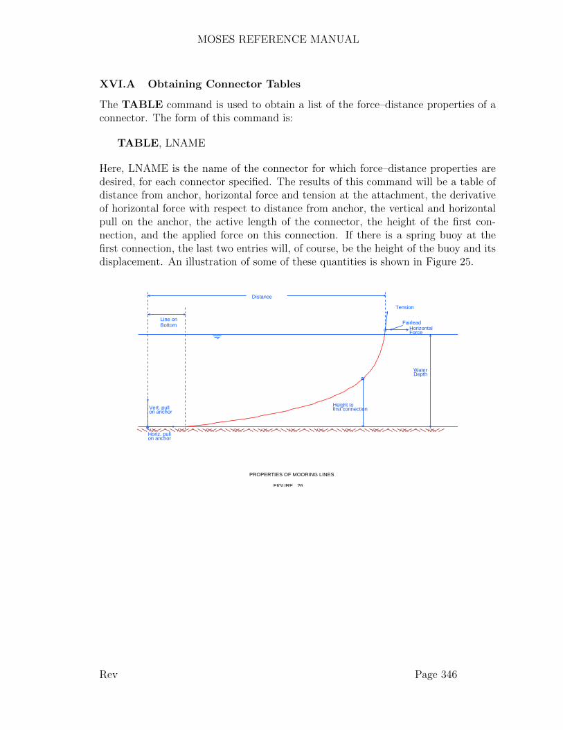
MOSES REFERENCE MANUAL
XVI.A Obtaining Connector Tables
The TABLE command is used to obtain a list of the force–distance properties of aconnector. The form of this command is:
TABLE, LNAME
Here, LNAME is the name of the connector for which force–distance properties aredesired, for each connector specified. The results of this command will be a table ofdistance from anchor, horizontal force and tension at the attachment, the derivativeof horizontal force with respect to distance from anchor, the vertical and horizontalpull on the anchor, the active length of the connector, the height of the first con-nection, and the applied force on this connection. If there is a spring buoy at thefirst connection, the last two entries will, of course, be the height of the buoy and itsdisplacement. An illustration of some of these quantities is shown in Figure 25.
Tension
HorizontalForce
Fairlead
Height tofirst connection
Horiz. pullon anchor
Vert. pullon anchor
WaterDepth
Line onBottom
Distance
PROPERTIES OF MOORING LINES
FIGURE 26
Rev Page 346

MOSES REFERENCE MANUAL
XVI.B Obtaining Connector Geometry
The GEOMETRY command is used to obtain the current geometry of a connector.The form of this command is:
GEOMETRY, LNAME
Here, LNAME is the name of the connector for which the geometry is desired. Theresults of this command will be a table of the distance along the connector from ”end2” to the point in question, the horizontal distance from end 2 to the point, and theX, Y, Z, coordinates of the point. After the properties are computed, the user isplaced in the Disposition Menu.
Rev Page 347
MOSES REFERENCE MANUAL
XVI.C Finding the Restoring Force
The MOVE command is used to obtain the restoring force on a body as a functionof either excursion or angle. The form of this command is:
MOVE, BODY NAME, –OPTIONS
and the available options are:
–LINE, TH, DIST, NUMBER–ROTATE, EXCUR, TH INC, NUMBER
where BODY NAME is the name of the body to be moved. If this is omitted, thecurrent body will be used. If no options are specified, then the default is the sameas –LINE with no data.
The option –LINE is used to move the body in a line. Here, TH is the direction (deg.)in which the body will be moved, measured from the global X axis positive towardglobal Y, DIST is the total distance of the move, and NUMBER is the number ofpositions calculated. Notice that the position increment is the quotient of the distanceand the number of positions. If only the body name is specified, then this commandwill move the body in thirty (30) equal increments in the direction TH from theinitial configuration until a termination criteria is met. This criteria is when themost heavily loaded line has a horizontal force equal to the maximum in the table.
The –ROTATE option is used to move the body around in a circle. Here, EXCURis the distance from the initial position (feet or meters) and this will be a constant.TH INC and NUMBER are the angle increments (deg.) and the number of anglesrespectively. If these are omitted, 10 degrees and 36 will be used.
At each position, the X and Y components of the restoring force and the magnitudeof the restoring force are reported. Also, the tension, the horizontal force, and ratiowill be reported for the lines with maximum and minimum tensions. During thisprocess, all other bodies are held fixed in their position in the initial configuration.
Rev Page 348

MOSES REFERENCE MANUAL
XVI.D Obtaining the Results for a Pile
To aid in designing or checking a pile, MOSES has the command:
PILE DESIGN, PILE NAME, –OPTIONS
where the options are
–FORCE, FX, FY, FZ, MX, MY, MZ–DISPLACEMENT, DX, DY, DZ, RX, RY, RZ
When this command is issued, MOSES will take the pile defined by PILE NAMEand apply either a force or a displacement at the top of the pile. A force is specifiedby the –FORCE option where forces and moments are specified in the global coor-dinates in bforce and bforce–blength. An imposed displacement is specified via the–DISPLACEMENT option and is defined in the global system (inches or mm anddeg.).
When this command is issued, MOSES will iterate a solution for the pile with theconditions specified. At the conclusion of the computation, the user is placed inthe Disposition Menu where he may dispose of the results as he sees fit. Whenreporting these results, three different reports are available: LOCATION, FORCE,and STRESS.
Rev Page 349

MOSES REFERENCE MANUAL
XVI.E Designing a Lifting Sling
To aid in the design of a lifting sling, MOSES has a special command:
SLING DESIGN, *NOD(1), ..., *NOD(4), BEGHEI, MAXHEI, NUM
When this command is issued, MOSES will take the body to which the nodes areconnected in the initial configuration and compute the lengths of each element ofthe sling so that the hook point is above the center of gravity. This computationis made for a hook height beginning at BEGHEI for NUM heights (feet or meters),measured from the highest sling attachment point until the height exceeds MAXHEI.At each height step, the tensions in each sling element are estimated so that the hookload equals the body weight. The height step increment is calculated as (BEGHEI–MAXHEI)/(NUM–1).
At the conclusion of the computation, the user is placed in the Disposition Menuwhere he may dispose of the results as he sees fit.
Rev Page 350

MOSES REFERENCE MANUAL
XVI.F Obtaining Propulsion/Weather Envelopes
The PROPULSION command is used to obtain an envelope of the maximum wind,current, and wave which yields one propulsion unit having maximum thrust. Theform of this command is:
PROPULSION, CNAME
Here, CNAME is the name of the control assembly which will be checked. Whenissued, this command will use the current environment and iterate a the maximumwind, wave and current. These will be done in order so that the results will be themaximum maximum environmental component which can act with the others at theirnominal values. For example, suppose that the current environment is defined with
&ENV –WIND 100 90 –CURRENT 3.0 45 –SEA ISSC 135 10 7
The results of this comand will be a table with four columns labeled Heading, MaxWind, Max Current, and Max Wave. The column labeled Max Wind is the maximumwind speed at 90 degrees acting in concert with a current of 3 at 45 degrees and a seaof significant height of 10 at 135. These are reported as a function of vessel heading.
Rev Page 351
MOSES REFERENCE MANUAL
XVII. THE REPOSITION MENU
To investigate different ways to reposition bodies using connectors, MOSES providesthe Reposition Menu. This menu is entered using the command:
REPO
and must be exited using an
END REPO
command. At this menu level, several commands are available to specify prefer-ences for performing the repositioning, display the selected values, and perform therepositioning. These commands are:
DO REPOWEIGHT CONN, WT, :SC(1), :SC(2), ..., :SC(n)BOUNDS CONN, UB, LB, :SC(1), :SC(2), ..., :SC(n)SELECT CONN, :SC(1), :SC(2), ..., :SC(n)DESIRE VALUE, DES, :SC(1), :SC(2), ..., :SC(n)TUG DCHANGE, WFMUL, WDMUL, :TS(1), :TS(2), ..., :TS(n)SHOW SYS
The DO REPO command instructs MOSES to find new line lengths and tug forcesso that the system will be in equilibrium at the current position, subject to thecontrols specified with the other commands. This problem will not always have asolution as specified and it is up to the user to check that he finds the results suitablefor his purpose.
This command changes only those connectors selected by the latest SELECT CONNcommand, and will keep the tensions (tug forces) between the upper and lower boundsas specified for each connector using BOUNDS CONN. Here, UB is the upperbound, while LB is the lower bound, both in bforce units. The equilibrium so-lution keeps the force in each connector as close as possible to the desired value,DES (bforce), defined with DESIRE VALUE. The command WEIGHT CONNis used to specify the relative desirability of changing a given connector. With thiscommand, WT is the relative weight factor to be used for the specified connectors.For all these commands, :SC(n) and :TS(n) refers to a selection criteria containingconnector names, or can refer to the connector name itself. The SHOW SYS com-mand will produce a report showing the selection status, current force, desired force,upper and lower bounds, and the weight value for each connector.
Normally, MOSES will change force in tugs instead of changing their direction. The
Rev Page 352

MOSES REFERENCE MANUAL
command TUG DCHANGE allows for a tug to change direction as well. Here,WFMUL and WDMUL are the relative desirability factors for changing force anddirection, respectively.
Rev Page 353

MOSES REFERENCE MANUAL
XVIII. THE HYDROSTATIC MENU
To perform hydrostatic computation with MOSES, one should issue the command
HSTATICS, BODY NAME
from the main menu. This command will place the user in the Hydrostatics Menu,where he can compute hydrostatic results for a single body. The body which will beconsidered will be either the current body, or the one specified on the HSTATICScommand. In this menu, MOSES can perform four classes of hydrostatic analysis:
• Curves of Form,• Righting Arm Curves,• Damage Stability• Longitudinal Strength, and• Tank Capacities.
Unless specified, the results obtained will be computed assuming that the watersurface is flat. To consider the effect of a wave, one can use the option:
–WAVE, WLENGTH, STEEP, CREST
on any of the commands in this menu. Here, WLENGTH is the length of the staticwave (feet or meters), STEEP is the reciprocal of the wave steepness, and CRESTis the distance of the crest from the vessel origin (feet or meters). Notice that thewave height here is obtained by MOSES as the quotient WLENGTH/STEEP. Oncespecified, the wave will remain in effect until it is nullified by specifying a –WAVEoption with zero height.
As far as MOSES is concerned, there is no difference between hydrostatic proper-ties for an intact vessel and a damaged one. There are simply a different set ofactive compartments for one analysis than for another. As an example, supposethat one had just performed a set of righting arm computations for an intact ves-sel. To perform a similar analysis for a damaged condition, he would simply issue a&COMPARTMENT –FLOOD :TNK command to tell MOSES which tanks orcompartments he wished to flood. Next, he would issue the EQUI command to findthe floating damaged position, and then issue a RARM command to examine thestability of the damaged system.
Rev Page 354

MOSES REFERENCE MANUAL
XVIII.A Tank Capacities
To compute tank capacities, the user should issue a command of the form:
TANK CAPACITY, TNAME, INC, –OPTIONS
Where the options available are:
–ROLL, ROLL ANGLE–PITCH, PITCH ANGLE
When this command is issued, MOSES will compute the weight, volume, and centerof the compartment name TNAME in increments of INC (feet or meters). Normally,it is assumed that the vessel has zero roll and pitch. This can be changed, however,with either of the two options. The angles one specifies here are in degrees. At theconclusion of the command, the user is again placed in the Disposition Menu so thathe can dispose of the results.
Rev Page 355
MOSES REFERENCE MANUAL
XVIII.B Curves of Form
Perhaps the most primitive hydrostatic results are those which normally comprisethe curves of form. To generate this type of result with MOSES, one should issue theCFORM command. After the properties have been computed, MOSES will placethe user in the Disposition Menu so that he can dispose of the results as he desires.This command produces two hard copy reports in the Disposition Menu: BASICand COEFFICIENT. The first of these contains the condition, displacement, centerof buoyancy, waterplane area, center of flotation, and the metacentric heights. Thesecond contains the condition, the wetted surface, the load to change draft, and themoment to trim. If no data is specified on the REPORT command in the DispositionMenu, then both reports will be printed.
The form of the command for curves of form is:
CFORM, DRAFT, ROLL, TRIM, –OPTIONS
and the available options are:
–DRAFT, INC, NUM–ROLL, INC, NUM–PITCH, INC, NUM–WAVE, WLENGTH, STEEP, CREST
Here, the initial draft, roll, and trim are specified by DRAFT, ROLL, and TRIM,and the number of conditions and the increment are defined by one of the first threeoptions. If the –DRAFT option was specified, then draft will be incremented by INC(feet or meters) NUM times. Similar results are obtained with either –ROLL or –PITCH, except that here INC is in degrees and roll and/or pitch will be incremented.Finally, the –WAVE option controls the static wave{!!li} as discussed previously.
Rev Page 356

MOSES REFERENCE MANUAL
XVIII.C Finding Floating Equilibrium
The method for finding an equilibrium position is fundamental to the manner inwhich MOSES considers hydrostatics. Instead of using a specified draft and trim todetermine the weight, ballast, and cargo for a vessel system, MOSES allows the userto input these weights and ballasts directly via internal commands discussed earlier.After the system has been defined, the question remains as to where the vessel willfloat. This question can be answered by issuing the following command:
EQUI H, –OPTIONS
and the available options are:
–ECHO, YES/NO–FIX, DOF(1), ..., DOF(N)–NUMITER, ITER MAX–TOLERANCE, HE, RO, PI–WAVE, WLENGTH, STEEP, CREST
When this command is issued, MOSES will iterate until equilibrium is found. Theprogram simply iterates until the center of buoyancy is above or below the center ofgravity, and the buoyancy equals the weight. If one wishes to see the details of theresulting position, he should issue the &STATUS command afterward.
The –ECHO option controls the trace of iterations which is printed at the terminal.If YES/NO is YES, then the trace will be printed, otherwise it will not. The option–FIX fixes the specified degrees of freedom during the iteration. Here, DOF(i) canbe HEAVE, ROLL, and/or PITCH. The option –NUMITER is used to overridethe default (20) number of iterations, and –TOLERANCE is used to override thedefault closure tolerances for heave, roll, and pitch respectively. The values are apercentage of weight for heave, and arms for the angular motions. The defaults are0.0001, 0.01, 0.01. Finally, the –WAVE option controls the static wave as discussedpreviously.
Rev Page 357
MOSES REFERENCE MANUAL
XVIII.D Longitudinal Strength
To produce longitudinal strength results, the user should issue the command,
MOMENT, –OPTIONS
where the available options are:
–WAVE, WLENGTH, STEEP, CREST–ALLOW, ALLOW STRESS, ALLOW DEFLECT
When it is issued, MOSES will include all applied loads, the ballast in all tanks, thedefined weight, and the buoyancy in the strength calculations. The values used for thebuoyancy are those of the current state, i.e., the buoyancy is computed consideringall parts which are active, and the current draft, roll, and trim. The current statecan be set with either an &INSTATE, EQUI H, or &EQUI command.
It is possible that the shear curve will not close, particularly if the vessel is not in staticequilibrium. To close the shear curve, one should either issue an EQUI H, &EQUI,&WEIGHT –COMPUTE, or &CMP BAL command, to establish equilibriumbefore issuing the MOMENT command. If one is interested in longitudinal strengthin waves, he should issue EQUI H with the –WAVE data before the MOMENTcommand. If not, the vessel will normally not be in equilibrium and the shear curvewill not close.
In applying the loads, the default procedure is to include a load even if all of itsdistribution is not applied within the geometric limits of the vessel. When this occurs,the overhanging part of the load is transferred as an applied load and moment at thevessel end. If the end of the load is forward of the beginning, the end is set tobe very close to the beginning. When a load is completely off of the vessel, it isapplied as a concentrated load and moment at the end, and again the shear andmoment curves will not close. After the results have been computed, the user isplaced in the Disposition Menu so that he can dispose of the results generated. The–ALLOW option is used to define the allowable deflection and stress in the vessel.Here ALLOW STRESS is the allowable stress (ksi or mpa), and ALLOW DEFLECTis the allowable deflection (inches or mm).
Rev Page 358
MOSES REFERENCE MANUAL
XVIII.E Righting and Heeling Arm Curves
To compute righting and heeling arm results, the user should issue a command of theform:
RARM, INC, NUM, –OPTIONS
The options available are:
–ECHO, YES/NO–FIX–NUMITER, ITER MAX–TOLERANCE, HE, RO, PI–WAVE, WLENGTH, STEEP, CREST–YAW, YAW ANGLE–WIND, WIND SPEED–CEN LATERAL, X, Y, Z–U CURRENT, FLAG–W COEFF, WC0, WC1, WC2, WC3–R COEFF, RC0, RC1, RC2, RC3–STOP, HOW–WEIGHT, SF WEIGHT
The –ECHO option controls the trace of iterations which is printed at the terminal.If YES/NO is YES, then the trace will be printed, otherwise it will not. The option,–FIX, fixes the trim of the vessel during the iterations. The option –NUMITER isused to override the default (20) number of iterations, and –TOLERANCE is usedto override the default closure tolerances for heave, roll, and pitch respectively. Thevalues are a percentage of weight for heave, and arms for the angular motions, andthe defaults are 0.0001, 0.01, 0.5. Finally, the –WAVE option controls the staticwave as discussed earlier.
When the command is invoked, it will rotate the vessel NUM times adding INC tothe roll angle. For each increment, the program will iterate an equilibrium positionfor the other degrees of freedom and then compute the righting and wind heelingarms. Since the righting arm is based on the equilibrium of the buoyancy and weightof the vessel, the vessel weight must have been previously defined either in the modelitself, or via an &WEIGHT command. For this command only, roll is defined as arotation about an axis which can be changed. The default is, of course, the vessel Xaxis.
The –YAW option is used to compute righting arms about a skewed axis. YAW ANGLEis the angle of the axis for computing the arms from the vessel X axis. If this option
Rev Page 359
MOSES REFERENCE MANUAL
is used, then the axis for the ”roll” is yawed to the angle specified. Here, the angleis measured positive from the X axis positive toward Y. If one uses a angle of 90degrees, the ”roll” axis will be moved 90 degrees toward Y and the righting arms willbe about the Y axis. In other words, here a ”roll” of 2 degrees will make the vesselstern go down.
In addition to computing the righting arms of the vessel, MOSES will compute thewind heeling arms when the –WIND option is used. Here, any load attributes whichattract wind (#AREA, #PLATE, #TABLE, #TANKER, structural elements, orpieces) will be used with WIND SPEED (knots) to compute a wind force. A heelingmoment is computed from this force and an assumed point of application. There arethree alternatives here:
• By default, MOSES assumes that the force is equilibrated by a pressure dis-tribution which has a center of pressure at the vessel center of buoyancy. Forcertain types of vessels, this assumption may not be applicable.
• This center can be specified using the –CEN LATERAL option. Here, X, Yand Z are the coordinates of the center of lateral resistance in the local bodysystem.
• Finally, the Current Model can be used to compute the assumed applicationpoint. To utilize this method, one simply specifies the option –U CURRENT.MOSES will then compute a current force on the vessel which equilibrates thewind force and use this to compute the application point. If FLAG is INITIAL,then the application point will be computed at the first condition and the samepoint used for all other conditions. If FLAG is any other value, MOSES willcompute the application point for each heel angle. This probably should be thedefault, but it requires a proper drag model.
The –W COEFF and –R COEFF options allows one to define a ”heeling/restoringmoment” which will be added to that computed from the load attributes. Here, WC0,WC1, WC2, and WC3 or RC0, RC1, RC2, and RC3 define that additional momentsas:
MW = ( WCO + WC1 * H + WC2 * H*H + WC3 * H*H*H) * WIND SPEED**2
MR = ( RCO + RC1 * H + RC2 * H*H + RC3 * H*H*H)
where H is the roll angle in degrees, and MW is in bforce–blength, and MR is in feet
Rev Page 360

MOSES REFERENCE MANUAL
or meters.
The –STOP option is used to stop the computation after a specified event hasoccurred. If HOW is RARM then it will stop when the righting arm crosses zero.For a value of NET, termination will occur at the second intercept point. Finally,DOWN will terminate when the minimum NWT down–flooding height becomesnegative.
One of the results computed during this process is the minimum height of all down–flooding points on the vessel. The user can define and alter this set of points with&DESCRIBE COMPARTMENT commands. If he has not defined a point, thenthe height of the vessel origin will be reported. The –WEIGHT option is usedto redefine the scale factor used to convert righting moments into righting arms.By default, the apparent weight of the vessel is used. If the option is exercised,SF WEIGHT (bforce) will be used.
At the conclusion of the command, the user is again placed in the Disposition Menuso that he can dispose of the results.
Rev Page 361
MOSES REFERENCE MANUAL
XVIII.F Stability Check & Allowable KG
Stability is a simple concept but is extremely complicated in practice. To simplifyassessing stability, MOSES has two commands STAB OK and KG ALLOW. Whatthey do is compute several things from the basic results reported by the RARMcommand; and if you ask it to, it will check to see if the value computed is greaterthan a specified value. These checks are given by the stability criteria of the differentregulatory bodies.
All angles (except the equilibrium angle) defined below are relative to the equilibriumposition. First, let us define the symbols:
• R(a) = The righting arm at the angle a.• H(a) = The wind heeling arm at the angle a.• RA(a) = The area under the righting arm at the angle a.• HA(a) = The area under the wind heeling arm at the angle a.• DWT = The smallest angle at which a WT point goes below the water.• DNWT = The smallest angle at which a NWT point goes below the water.
The angles are shown in the figure below.
Now, the macros compute:
• GM = The distance from the metacenter to the center of gravity.• DOWN H = The down–flooding height at equilibrium.• ZCROSS = The equilibrium angle without wind.• THETA1 = The first angle, T, at which R(T) = H(T).• THETA2 = The second angle, T, at which R(T) = H(T).• RANGE = (of stability) Is the second angle, T, at which R(T) = 0.• R M EQUI = The RANGE – FACTOR * ZCROSS. Here, FACTOR is specified
on the option.• DANG = DNWT.• DANG T1 = DNWT – THETA1.• DWT T1 = DWT – THETA1.• ANG DIFF = THETA2 – THETA1.• ANG@MARM = The angle at which the RA peaks.• AR RATIO = The ratio of the RA/HA with both measured at the minimum
of DANG and THETA2.• ARR@30 = The ratio of the RA/HA with both measured at the minimum of
THETA2, DANG, or 30 degrees.• AR RESID = RA(T) – RA(THETA1) – [ HA(T) –HA(THETA1) ] where T is
the smallest of the down flooding angle, or the second intercept.• RARM@30 = R(30).
Rev Page 362

MOSES REFERENCE MANUAL
Rev Page 363

MOSES REFERENCE MANUAL
• ARM AR = RA(THETA2).• ARE@DFLD = min ( RA(DANG), RA(THETA2 )• ARE@MARM = RA(M) where M is the angle where R is a maximum.• ARE@30 = RA(T) where T is minimum of 30 degrees, DANG, or THETA2.• ARE@40 = RA(40d), where 40d is the minimum of 40 degrees, DANG, or
THETA2. degrees.• AREBTW = RA(40d) – RA(30), where 40d is the minimum of 40 degrees,
DANG, or THETA2.• ARM RATIO = R(M)/H(M) where M is the minimum of DANG, THETA2,
or the angle of maximum righting arm.• AR WRATIO = [ RA(TW) – RA(MANG) ] / AD, Here the heeling arm is
assumed to be a constant HAW = 1.5 * HA(0). Now, TW is the second interceptof the constant wind arm and the righting arm, AD = HAW * [TW + TT], andTT = MANG – T1. Here we use the RA at a positive MANG even though theangle is drawn as negative on the figure. This is equivalent to assuming thatRAA is skew symmetric about the origin.
For checking intact stability, the two commands discussed below will accept thefollowing options.
–I GM, IGM–I AR RATIO, IARATIO–I RARM@M30, IRARM@M30–I AR WRATIO, IAWRATIO, MANG–I ARM RATIO, IARMRAT–I DOWN H, I DOWNH–I ARE@MARM, IARE@MARM–I ARE@DFLD, IARE@DFLD–I ARE@30, IARE@30–I ARE@40, IARE@40–I AREBTW, IAREBTW–I ARM AR, IARMARE–I AR RESID, IARRESID–I ZCROSS, IZCROSS–I THETA1, ITHETA1–I RANGE, IRANGE–I R M EQUI, IRMEQUI, FACTOR–I ANG DIFF, IANGDIF–I DANG T1, IDANGT1–I DANG, IDANG
Rev Page 364

MOSES REFERENCE MANUAL
–I ANG@MARM, IANG@MARM
Here, what follows the –I is the quantity defined above and the second thing is whichwill be compared to the computed quantity. Two of the options require a secondvalue. AR WRATIO needs MANG, the nominal roll due to waves, and R M EQUIneeds the FACTOR to multiply THETA1. These options will be used to check intactstability. There is a second set of option which begin with –D which are used tocheck damaged stability. For example:
–I GM, 5, –D GM 1
will demand that the GM exceed 5 for an intact case and 1 for a damaged case.
STAB OK produces the righting arm, heeling arm, and area ratio curves for thedraft specified. Since the righting arm is based on the equilibrium of the buoyancyand weight of the vessel, the vessel weight must have been previously defined. Thiscan be accomplished with the stanza:
$$********************************* set transit condition$&INSTATE –CONDITION 7$$********************************* compute weight for condition$&WEIGHT –COMPUTE 5 32 85 85
Now, stability checks with the commands of the form:
$$************************************** check one intact$
hystatstab ok 5 2.5 10 –wind 100 –yaw 0
$$************************************** check one damaged$
stab ok 5 2.5 10 –wind 100 –yaw 0 –damage 5p
These two checks are identical, except that the first one checks intact stability for a
Rev Page 365
MOSES REFERENCE MANUAL
draft of 5 feet, while the second one checks stability with compartment 5p damaged.
When using STAB OK (or KG ALLOW discussed below), the NWT DOWN pointsare used to check intact stability, and both the NWT DOWN and WT DOWN pointsare used to check damaged stability. The general form of the command is:
STAB OK DRAFT RANG INC NR ANGLES –OPTIONS
where the options are:
–R TOLERANCE HE, RO, PI–YAW, Y ANGLE–DAMAGE, DAM CMP–WIND, WIND–THWAV, ANGLE WAVE–CEN LATERAL XC, YC, ZC–U CURRENT–COEF WIND, W COEF–COEF RARM, R COEF–WIND MAC–RARM MAC
+ any of the options discussed above.
The variable DRAFT sets the draft for which stability will be checked. When thecommand is invoked, it will rotate the vessel NR ANGLES times adding RANG INCto the roll angle. For each increment, the program will iterate an equilibrium positionfor the other degrees of freedom and then compute the righting and wind heeling arms.
The –R TOLERANCE option is the same as the one on the RARM command.The values specified here will be passed to RARM whenever it is called. Likewisethe –YAW is analogous to the same option on the RARM command and is usedto compute righting arms about a skewed axis. The –DAMAGE option is used toselect tanks that will be damaged for damaged stability. If one does not wish to checkdamaged stability then this option should not be used.
The next set of options control the computation of wind heeling. The –WINDoption is used to define the wind which will be considered. The –CEN LATERAL,–U CURRENT, –COEF WIND and –COEF RARM options simply pass theirdata directly to the RARM command, so that their data is the same as that for theoption to the RARM command of the same name.
To include the roll owing to wave action, a wave angle can be included with –
Rev Page 366
MOSES REFERENCE MANUAL
THWAV. The righting and wind arm calculations will begin at the angle AN-GLE WAVE to windward.
Alternatively, the –WIND MAC option will call the macro
COEF SET yaw draft
and the –RARM MAC option will call the macro
COEF RSET yaw draft
immediately before each invocation of RARM. If you use this option, then you mustwrite the macro, COEF SET or COEF RSET. It takes the two arguments and set avariable. An example is:
&MACRO COEF SET YAW DRAFT&SET COE WIN = –W COEF A B C D
&ENDMACRO&M ACT COEF SET RARM
&MACRO COEF RSET YAW DRAFT&SET COE WIN = –R COEF A B C D
&ENDMACRO&M ACT COEF RSET RARM
One can add any logical he wishes here to change the coefficients based on draft andyaw. The values A, B, and C are numbers depending upon the situation.
By default, righting arms are computed about the equilibrium position which iscomputed before starting. If the –NO EQUI option is used, the basic position isused. Notice that the GM may not be defined when using this option.
The results of this command are plots of the righting arm, heeling arm, area ratiocurves, and two reports. The first report is the standard stability report. The secondpresents: the condition, the allowables, and the results for each stability criterionalong with a statement of ”PASS” or ”FAIL”.
We apologize for the complexity here, but we tried to make these commands applica-ble to as many rules as possible. Only the checks which are specified will be checkedand reported.
We compute the maximum allowable KG for a set of drafts, intact wind speed, and
Rev Page 367

MOSES REFERENCE MANUAL
a damage wind speed with the command:
KG ALLOW
where the options are:
–WIND, I WIND, D WIND–YAW, Y ANGLE(1), .....–DAMAGE, DAM CMP(1), .....–DRAFTS, D1, D2, ......–KG TOL, KG TOL–KG MIN, KG MIN–KG MAX, KG MAX–CEN LATERAL XC, YC, ZC–U CURRENT–COEF WIND, W COEF–WIND MAC
+ any of the options discussed above.
The options here are ”the same as” those for the STAB OK command, except thatone should specify wind speeds for both intact and damaged cases with –WIND andone can specify more that one thing with –YAW and –DAMAGE. The only newoptions are –KG TOL which define the tolerance (feet or meters) for the compu-tation of the allowable KG, –DRAFTS which defines the drafts to be considered,–KG MIN, and –KG MAX. The last two of these are used in setting the limitswhich will be searched and normally should not be needed. KG MIN has a defaultof 0 and thus it is assumed the vessel has been coded up according to the documen-tation or that if the KG is at the keel, the vessel will pass the stability requirements.If you get a message that ”LOWER BOUND FAILS”, then you need to use this op-tion with some negative KG so that the message goes away. The –KG MAX valuedefaults a value which yields zero GM. If you have a partial run which establishes anupper bound on the allowable KG, you can use it here to minimize the computationaleffort.
For each draft specified, the command will find an ”allowable KG” for the set ofdamages and yaw angles specified. By allowable, we mean that any KG greater than(to within KG TOL) that found will fail one of the stability requirements for somedamage and yaw angle. Basically, this command simply incorporates an iterativealgorithm and repeatedly calls STAB OK to find the allowable. The command usesthe following search technique:
• It first sets a lower bound, KL, to MIN KG and checks to make sure that this
Rev Page 368

MOSES REFERENCE MANUAL
passes all cases (intact and all damages for all yaws).• It then sets the upper bound, KU, to about where the GM is MIN GM or that
specified with –MAX KG.• An estimate of the KG, KC, is obtained as a*KL+b*KU, and each cases is con-
sidered; i.e. for each intact and damaged condition, each yaw angle is considereduntil one fails or all pass. Here, a and b are chosen based on the number ofcases to be considered (number of damage compartments + 1 times the numberof yaw angles). The reason for doing this is that it costs much more to check acondition that passes than it does to check one that fails! Thus, the coefficientsare chosen to minimize the total cost of the search.• If all pass, the KL is replaced by KC and the above process is repeated.• If one fails, KU is replaced by KC and the process is repeated.• This continues until KU – KL is less than TOL and the allowable is taken to
be KL.• All of the above was done with no reporting. After an allowable KG has been
found, all of the cases are again considered and a report of the stability areprinted.
If more than one draft was specified, a plot of the allowable KG vs draft will bemade. Since the algorithm favors failure, it is much more efficient if you order thedata ”properly”. In particular, you should input the damage cases in order of mostlikely failure. The same can be said of the yaw angles.
Rev Page 369

MOSES REFERENCE MANUAL
XIX. THE HYDRODYNAMIC MENU
The Hydrodynamics Menu contains commands which allow the user to build, alter,and maintain databases of hydrodynamic properties which act on body panels. TheHydrodynamic Database provides MOSES with the ingredients used in almost alltypes of analysis. This database can be input directly in this menu, or it can becomputed from the model. The menu is entered with
HYDRODYNAMICS
and when one has completed his task here, he exits with
END HYDRODYNAMICS
In order to fully understand the implications of the pressure database, it helps to havesome information about what the program computes and how it uses the intermediateresults. Basically, the primitive quantity is a set of velocity potentials on each panelwhich results from the interaction of the panel with the sea. The first six of thesevelocity potentials arise due to unit motion of the body, at a given frequency, ineach of the degrees of freedom. These are called radiation velocity potentials. Theremaining potentials result from a wave being stopped by the body. These are calleddiffraction potentials. The diffraction potentials depend not only on wave frequencybut also on wave heading. All of the potentials are complex numbers ( a real and animaginary part for each potential ). Collectively, we will refer to these potentials as”diffraction results” since they are normally computed via some type of diffractionanalysis. The forces on Morison’s Equation elements are not a part of the pressuredatabase, are computed whenever they are needed, and are not considered in thisMenu. In addition to the diffraction potentials, the ”incident wave potentials” arealso required, but since they are easy to compute, they are not stored in the pressuredatabase. Also, for some computations, MOSES needs to have not only the potentials,but their gradient, so they are included in the database.
From these basic ingredients, MOSES then computes a new, or ”Total” databasewhich includes:
• The forces which unit amplitude regular waves exert on a stationary body,• The bodies’ added mass and damping matrices.• The mean drift force which a regular wave exerts on a stationary body,• The change in mean drift force with a motion of the body, and• The damping on a body due to time variation of the mean drift force.
Rev Page 370
MOSES REFERENCE MANUAL
These results are a function of wave heading, forward speed, and encounter frequency.
The Hydrodynamic database actually consists of two different types of data for eachbody: Pressure data and Mean Drift Force Data. Also, the data is stored by ”PacketName”. Thus it is possible to have several different sets of hydrodynamic data avail-able for each body. For example, one can have different sets for different draft andtrim conditions, or different sets computed with different methods. A packet of datais associated with body whenever the packet is: Generated, or Imported. In general,the user is free to define the packet name for the data when it is created, but if thename already exists, then a new name will be created. The same name can exist foreach of the different types of data, but all names for a given type of data must beunique. A special reserved packet name is NONE. If this name is associated with abody for a given type of data, then it has the same effect as null data.
The data in the Hydrodynamic database is used in both frequency and time domaincomputations. Since the database consists of frequency domain quantities, its use inthe frequency domain is easily inferred. For a time domain simulation, use of thisdata is not obvious. Here, three things happen. First, an excitation force is createdas a cosine series of the frequency domain forces. The periods for the series are thosespecified with the –S PERIOD option on the &ENV command. The amplitudes arechosen to conform to the specified sea spectrum, and a set of phases are chosen. Next,a mean drift force is computed from the drift force ”RAOs” and the sea spectrum.A time varying drift force is created as a cosine series at periods specified with the–MD PERIOD options of the &ENV command and amplitudes which conform tothe drift spectrum and a set of phases. Finally, the frequency domain added mass anddamping matrices are transformed by an inverse Fourier transform into a convolutionkernel, or ”retardation function”, and the equations of motion are integro–differentialequations. Thus, any time domain simulation in a seaway first requires the basic datadiscussed above.
The basic method of computing mean drift force from the hydrodynamic pressuresis to integrate the results over each submerged panel. If, however, one has used striptheory, then this results in zero surge drift force (the surge diffraction potential isignored). In this case, a representation by Salvesen which employs an assumption ofthe body being a ”weak scatterer” is used to estimate a surge component.
There are basically two types of data considered in this menu: pressure and meandrift. Each of these will be considered in detail later, but as a general rule commandswhich generate data begin with G , those which post–process with V , those whichimport with I , and those which export with E . The commands for importing hydro-dynamic data are designed to allow the user to completely describe a hydrodynamicdata base. Although the commands for doing this are documented in the followingsections, the user is encouraged to examine the samples of data provided with this
Rev Page 371

MOSES REFERENCE MANUAL
software release. To input your own data, it is helpful to first export a hydrodynamicdata base to get an understanding of the MOSES file format. Then, modify this fileas desired, and import it to the program.
Rev Page 372
MOSES REFERENCE MANUAL
XIX.A Pressure Data
To compute the sea pressures on the vessel, the program must know the form of thevessel below the water. This is communicated to MOSES by a set of vessel descriptiondata, defined earlier, and the current condition of the body. To initiate the pressurecomputations discussed above, one must issue:
G PRESSURE, BODY NAME, PKT NAME –OPTIONS
and the available options are:
–HEADING, H(1), H(2), ...., H(n)–PERIOD, T(1), T(2), ...., T(n)–MAX DIST, DIST
When this command is issued, MOSES will take the system in its current configu-ration and compute frequency domain pressures and a total hydrodynamic databasefor the body BODY NAME. This data will be stored by the name PKT NAME inthe database.
The –HEADING option is used to change the default values of vessel headingfor which results will be computed. H(i) is the ith value of heading (deg.) to beconsidered. Here, heading is measured as an angle from the X axis, positive towardY. Hence, for a vessel described with the origin at the bow, head seas are 180 degrees.The –PERIOD option is used to alter the default values of encounter period, andT(i) is the ith value of encounter period in seconds. As many of these options asneeded can be input, so long as the number of periods does not exceed 200. Thedefaults for heading and period are set with options on &DEFAULT.
When the G PRESSURE command is issued, MOSES takes the vessel descriptionand the condition defined, and converts the vessel description into one describing thevessel below the waterplane. The program will then compute the added inertia anddamping matrices, and the applied forces on the vessel. These computations willbe performed for the periods and headings defined by the command. In convertingthe model, the two options –M DISTANCE and/or –M WLFRACTION of the&PARAMETER command are used to refine the computation. Use of these op-tions allows one to define a quite crude mesh and have MOSES automatically refineit to achieve any desired degree of precision. Also, the option –MAX DIST pro-vides a way to get approximate solutions to large diffraction problems with reducedcomputational effort. This option defines a maximum distance (feet or meters) forpanel interaction. Any two panels which have a distance between them greater thanDIST will have a zero for their coupling terms in the diffraction matrix. For verylong slender bodies, this option can be used quite effectively to save computer effort.
Rev Page 373

MOSES REFERENCE MANUAL
For a body 4000 ft long with 6000 diffraction panels, answers within 10% of the exactones can be obtained in 66% of the time.
Once one has a pressure database, it can be examined in the Disposition Menu. Inparticular, the command
V MATRICES, BODY NAME
will gather the added mass and damping matrices for the pressure packet currentlyassociated with body BODY NAME and place the user in the Disposition Menu.Alternately, the command
V EXFORCES, BODY NAME
will do the same thing with the wave excitation forces. For both of these commands,the results are about the origin.
As mentioned earlier, it is possible to define the hydrodynamic pressure distributionand/or the total hydrodynamic database via commands. The same device is usedif one has computed hydrodynamic pressures and wished to ”save” them for uselater. This capability can be quite useful when analyzing a large diffraction model.For instance, one could alter the mooring lines of system, and use the importationfeature to save time in the reanalysis. Caution should be used here, so that onlychanges to the model that do not effect hydrodynamic properties are performed. Toemit a hydrodynamic database, one issues:
E PRESSURE, BODY NAME –OPTION
where BODY NAME is the name of the body for which hydrodynamic databases willbe emitted. This command will export a pressure database for the packets currentlyassociated with the body BODY NAME. Here, the only option is –NOTE which isjust like the same option on model definition commands. In particular, you need tospecify all five characters of the option, and the note that you attach will be includedas a comment in the emitted file. Also, the title and subtitle will be included if theyare not blank. No drift or total data will be emitted since it is recomputed when thepressure data is imported. It is possible to export (and subsequently import) a totalhydrodynamic database. This is accomplished with:
E TOTAL, BODY NAME –OPTION
The resulting output is substantially smaller than the pressure database. Here theoptions and titles are the same as for the pressure database. This file, however,consists data for both Total force and drift force. For simulation purposes, this is all
Rev Page 374

MOSES REFERENCE MANUAL
that is necessary, but it cannot be used for computing structural loads. When sucha database is input, a single warning to this effect will be given.
The format of an exported pressure database is the same as the one used to definethe data directly to MOSES. It begins with the command:
I PRESSURE, BODY NAME, PKT NAME, DISPL, –OPTIONS
which places the user in a submenu. Here, BODY NAME is the name of the bodyfor which the database is being generated, PKT NAME is a desired packet name,DISPL is the displacement at the condition being defined, and the options are:
–PERIOD, T(1), T(2), ......–HEADING, H(1), H(2), ......–CONDITION, DRAFT, ROLL, PITCH
Even though these items are called options, the first three of them are necessary toproperly define the database. The –PERIOD option defines the periods (sec) forwhich the database will be defined, and –HEADING defines the headings (deg) forwhich the exciting forces will be defined. The –CONDITION option defines thevessel condition for which the database is defined and DRAFT, ROLL, and PITCHare the draft (feet or meters), roll (deg), and pitch (deg) defining the condition. Theremaining options were described previously.
Once the menu has been entered, several commands are available. First, the com-mand:
FP MAP PANEL NAME, :PNT SEL(1), :PNT SEL(2), .......
defines a how the structural loads on the panel PANEL NAME will be mapped toall points matching :PNT SEL(i). The command:
FPANEL PANEL NAME, AREA, XC, YC, ZC, NX, NY, NZ, WLLEN
defines a panel. Here, PANEL NAME is the name of the panel, XC, YC, and ZCare the coordinates ( feet or meters ) of its centroid, NX, NY, and NZ are thecomponents of its normal, and WLLEN is the length of the intersection of the panelwith the waterline ( feet or meters ).
After a panel has been defined, the pressures acting on it are defined through a setof velocity potentials with commands:
FPPHI PER, RPRX, IPRX, RPRY, IPRY, .... \
Rev Page 375
MOSES REFERENCE MANUAL
RPRRZ, IPRRZ, RPDH(1), IPDH(1), ...
Here, PER is one of the periods T(i), and the remainder of the data are velocitypotentials per unit wave amplitude (feet or meters). These commands must be indecreasing order of period. In other words, the value of PER for a given commandmust be less than the value of PER for the previous one and greater than PER forthe next one. The velocity potentials are pairs of real and imaginary numbers. Thefirst six pair (twelve numbers) are the radiation potentials, and the remainder arediffraction potentials. The diffraction potentials correspond to the headings H(i),and are in the same order.
The final type of data for a panel is defined with:
FDELP PER, RPRXX, IPRXX, RPRXY, IPRXY, .... \RPRRZZ, IPRRZZ, RPDHX(1), IPDHX(1), ...
These quantities are the gradients of the potentials defined with the FPPHI com-mand, and thus there will be 3 times as many values as on the FPPHI command. Ifthese are viewed as complex numbers, then the first three numbers are the derivativeswith respect to X, Y, and Z of the first potential on FPPHI. The first 36 values (18complex numbers) are gradients of the radiation potentials. The gradients of thediffraction potentials follow for each heading.
After all of the panels have been defined, the menu is exited with an END I PRESSUREcommand.
To define a ”total hydrodynamic database” one first issues:
I TOTAL, BODY NAME, PKT NAME, DISPL, –OPTIONS
One can then describe the hydrodynamic data, and issue END I TOTAL to exitthe menu. Here, BODY NAME is the name of the body for which the database isbeing generated, DISPL is the displacement at the condition being defined, and theoptions are:
–PERIOD, T(1), T(2), ......–HEADING, H(1), H(2), ......–CONDITION, DRAFT, ROLL, PITCH–SCFACT, SCLEN, SCMASS, SCDRAG, SCFOR
Even though these items are called options, the first three of them are necessary toproperly define the database. The –PERIOD option defines the periods (sec), forwhich the database will be defined, and –HEADING defines the headings (deg), for
Rev Page 376

MOSES REFERENCE MANUAL
which the exciting forces will be defined. The –CONDITION option defines thevessel condition for which the database is defined and DRAFT, ROLL, and PITCHare the draft (feet or meters), roll (deg), and pitch (deg) defining the condition.
The option –SCFACT defines a set of scale factors which can be used to convertto the units required. In other words, all of the quantities input via the commandsdiscussed below will be multiplied by the scale factors prior to being stored in thedatabase. The manner in which these factors will be combined with the input num-bers will be discussed with each command.
After the I TOTAL command, the database is defined by a sequence of the followingcommands:
H ORIGIN, OX, OY, OZH EULERA, EROLL, EPITCH, EYAWH PERIOD, TH AMASS, AM(1,1), AM(2,1), ...., AM(6,6)H DAMP, DAMP(1,1), DAMP(2,1), ...., DAMP(6,6)H FORCE, H, RFKX, RFKY, ... RFKYAW, IFKX, ..., IFKYAW \
RDIX, RDIY, ... RDIYAW, IDIX, ..., IDIYAW \
The H ORIGIN and H EULERA commands define a change of coordinate systemfrom the one being input to the one employed by MOSES. Here, OX, OY, and OZare the components of a vector, in the MOSES body system from the origin in thelocal body system to the origin of the system in which the input quantities arecomputed. Likewise, the quantities EROLL, EPITCH, and EYAW are three Eulerangles (deg). These angles, when applied as a yaw followed by a pitch, followed bya roll, define the direction cosine matrix which transforms the system in which thequantities are computed to the local body system. If either of these two commands isomitted, the corresponding transformation will be assumed to be the identity. Oncea transformation has been defined, it will be used until it is redefined by anothersimilar command.
The H PERIOD command defines the period for all quantities which follow untila new H PERIOD command is encountered. Here, T is the period (sec) and itmust have been defined by the –PERIOD option on the I TOTAL command. Ifthe period defined by an H PERIOD command is the same as one previously used,the data following will be added to the previous data for the same period. Thus, onecan define the properties of a complicated body by inputting the properties for eachpiece of the body and letting MOSES combine them to form the properties of thebody.
The remaining commands are used to actually define the hydrodynamic properties
Rev Page 377

MOSES REFERENCE MANUAL
for the ”current” period, and they can be repeated as many times as desired until anEND is encountered. This marks the end of the hydrodynamic database definitionfor a given body.
The H AMASS and H DAMP commands define the added mass and linear damp-ing matrices respectively. The data is input on the command by columns of thematrix. The values which MOSES needs for the added mass matrix are added massdivided by displaced mass, and the length units should be feet or meters. Whenan H AMASS command is input, the top 3x3 is multiplied by SCMASS, the twocoupling 3x3 matrices are multiplied by SCMASS*SCMASS, and the bottom 3x3 ismultiplied by SCMASS*SCLEN*SCLEN, as defined with the –SCFACT option. Itis the product of the input values times the scale factors which should have the di-mensions defined above. The scaling for the damping matrix is similar to that for theadded mass except that SCDRAG is used instead of SCMASS. The desired units forthe product of the input values and the scale factors is damping coefficient dividedby displaced mass.
The H FORCE command defines the wave exciting force for the heading, H, whichhas been defined by the –HEADING option on the I TOTAL command. The firsttwelve values define the Froude–Krylov force, the next twelve define the diffractionforce. The first three values for each force will be scaled by SCFOR, and the lastthree will be scaled by SCFOR*SCLEN, as defined on the –SCFACT option. Theproduct of the input values times the scale factors should be either bforce, and feetor meters, depending upon the last &DIMEN command.
Rev Page 378
MOSES REFERENCE MANUAL
XIX.B Mean Drift Data
In most cases, the mean drift database is created as a consequence of creating thepressure database. This is simply the average of the nonlinear forces over time. Ingeneral, there are three contributions to this force: diffraction/incident potentials,radiation potentials, and the coriolis acceleration. The mean force due to diffrac-tion/incident potentials is independent of the motion while the other two depend onthe motion. Here, the last RAOs computed for the current process will be used tocompute theses contributions. The diffraction/incident and the radiation mean forcesare also used to apply a slowly varying force in the time domain as described earlier.The coriolis acceleration contribution to the mean is not used in the time domain.Instead, it is computed exactly.
One can examine the drift data with the command
V MDRIFT, BODY NAME
which will place one in the Disposition Menu to do whatever one wishes. Simpleestimates of the mean drift force can be created with the command
G MDRIFT, BODY NAME, PKT NAME –OPTIONS
and the available options are:
–MD TYPE, DTYPE–DIMENSIONS, LENGTH, BEAM, DRAFT–HEADING, H(1), H(2), ...., H(n)–PERIOD, T(1), T(2), ...., T(n)
Here, DTYPE must be either FORMULAE, or SEMI. The –DIMENSIONSoption defines the size (feet or meters) of the body used in estimating the drift. If itis omitted, the actual body dimensions will be used. The wave drift data computedhere is not sophisticated, and only mean drift is considered.
One can save a set of drift data for later use by issuing the command:
E MDRIFT, BODY NAME
which writes the drift data currently associated with body BODY NAME to a filefor later use.
The user can input his own drift database. To define mean wave drift responseoperators, one first enters a submenu with the command:
Rev Page 379

MOSES REFERENCE MANUAL
I MDRIFT, BODY NAME, PKT NAME –OPTIONS
and the available options are:
–HEADING, H(1), H(2), ...., H(n)–PERIOD, T(1), T(2), ...., T(n)
Here, PKT NAME is the name of the set of response operators, the –PERIODoption defines the periods (sec) and the –HEADING option defines the headings(deg) for which drift values will be defined. Once in the menu, the components ofthe mean wave drift force for the specified headings are defined with the command:
M DRIFT, PER, FXR(1), FXI(1), ...., FYAWI(1), ... \FXR(n), FXI(n), ..., FYAWI(n)
Here PER is the period for which this set of forces is applicable and must be one ofthe T(i) specified with the –PERIOD option. FXR(1), FXI(1), .. FYAWI(1) arethe real and imaginary parts of the mean drift forces and moments per unit of waveamplitude squared (bforce/blength**2 for force, bforce/blength for moments) for theheading HED(1). Likewise, the values FXR(2) ... are for heading HED(2), etc. Thecorrections to the mean force due to motions are a complex 6x6 matrix per waveamplitude**2 defined with the command:
MD MOTION, PER, HED, MDR(1,1), MDI(1,1), ... MDI(6,6)
the units here are feet or meters, bforce, seconds, and radians. When all of the datahas been defined, the menu should be exited with a END M DRIFT command.
Rev Page 380
MOSES REFERENCE MANUAL
XX. THE FREQUENCY RESPONSE MENU
Frequency response is a linear approximation to the equations of motion with assumedharmonic input. In MOSES, a menu is devoted to computing frequency response andits post–processing. To enter the menu, one inputs:
FREQ RESPONSE
When completed, the menu is exited with END FREQ RESPONSE.
The traditional way of obtaining frequency response is to consider a set of unitamplitude waves and to linearize the equations of motion for each wave. This isexactly what is done with the RAO command. Results obtained in this way can laterbe easily combined with different spectra to obtain approximations to the extremes inmany different situations, and are thus quite popular. The major disadvantage of thisapproach is that one can only look at the response to wave frequency excitation. Inother words, with the response operator approach, one cannot investigate the effectof wind or slow drift wave excitation. To cope with these other effects, one can nolonger look at unit amplitude waves, but must consider the simultaneous effect ofall environmental forces. This is what is done with the SRESPONSE command.The major disadvantage with spectral response is that this response is applicable toa single environment and thus the post processing options are limited.
Before getting into the details of these commands, a few general words are in order.The frequency response calculations depend not only on the sea pressures, but alsoon the stiffness of the connectors and the mass properties of the system. Instead ofrequiring the user to directly specify the weight and radii of gyration of the system,MOSES uses those computed from the element and weight data supplied in thestructural model, and from currently active tanks, weights, etc. This is necessaryto insure that when structural loads are computed, there will not be seriously outof balance in the loads. It is therefore important to accurately model the weightsnot only from a local sense, but also in a global one. Another important thing toremember is that the ”response operators” produced with the RAO command are notreally independent of wave height. For most cases, nonlinear damping (and perhapsforcing) is important. Thus, some real wave amplitude must be used to linearize thesystem. If post processing results are obtained for an environment which is radicallydifferent from that used in the linearization, then the applicability of the results isopen to question.
MOSES provides two ways to linearize the equations for RAO computations: specifiedwave amplitudes, and a spectral linearization. With the specified wave height method,one specifies a steepness, a period, and a wave height. This is the default method.MOSES will for each period and heading, use a constant wave steepness to obtain a
Rev Page 381
MOSES REFERENCE MANUAL
”real” wave amplitude for linearization for periods less than the specified period. Forlarger periods, the specified height will be used. The energy from the linear systemand the real system over a period are set equal to obtain the linearized results. Fordamping, this appears to be a rational approach. When, however, one looks at theforcing from a Morison’s equation element, it does not appear as attractive. Hereone is saying that the linearized coefficient depends only on the velocity for a singleFourier coefficient. The alternative is a ”spectral” linearization. Here, it is assumedthat the seas are unidirectional so that the RAOs for a set of periods and givendirection are linearized at one time. The spectrum is used to compute the RMS ofthe relative velocity at a point, and this is used to compute the ”drag” coefficient.The two approaches yield somewhat different results depending on the difference inthe peaks of the response and the spectrum. For SRESPONSE, the spectral methodis always used. However, the linearization here is not only over periods, but also overheadings.
In this light, it can be seen that frequency domain forces are no longer for zerospeed, and the interpretation of wave heading is different than before. That is, thefrequency domain forces are those used to compute the response. Sometimes these areforce/wave amplitude results (RAOs), and sometimes these are Fourier coefficients,depending on the use of SRESPONSE.
Response operators are computed by simply issuing the command:
RAO, –OPTIONS
where the available options are:
–HEADING, H(1), H(2), ...., H(N)–PERIOD, T(1), T(2), ...., T(N)–SPEED, VR–ITER, MAXIT–SPECTRUM, ENV NAME–STEEP, ST, PBCHEI, CHEI–ROD STEEP, ST, PBCHEI, CHEI
When this command is issued, MOSES will compute a new set of response operators,for the same frequencies and headings as those of the basic pressure data (thosespecified on the G PRESSURE command), unless the options –HEADING or–PERIOD are exercised. One can obtain response operators for any one speed byincluding the option –SPEED, where VR is the speed desired in knots.
If either –PERIOD or –HEADING are used, MOSES will interpolate values ofthe hydrodynamic forces, added mass, and damping from the values contained in the
Rev Page 382

MOSES REFERENCE MANUAL
pressure database. If no data for a quadrant exists in the pressure database, thenMOSES will assume symmetry about the vessel centerline or about amidships wheninterpolating hydrodynamic results.
The remaining options describe how MOSES deals with viscous damping. In gen-eral, there are three types of viscous damping which are considered: empirical rolldamping, Morison’s drag for bodies, and Morison’s drag for rod elements. Normally,MOSES will iterate up to thirty times to achieve a proper solution considering theviscous damping. In some cases where there are many bodies connected by rigidconnectors, there is a substantial computational effort involved with this iterativesolution. The –ITER option may be used to limit the number of iterations. Here,MAXIT is the maximum number of iterative steps which will be taken, where 30 isthe default value.
The –SPECTRUM option specifies the wave spectrum of the environment, ENV NAME,which will be used to linearize the equations spectrally. Here, any nonlinear de-pendence will be replaced by the RMS value times SMULT, where SMULT canbe specified with the –SPE MULTIPLIER option of an &DESCRIBE BODYcommand. If –SPECTRUM is omitted, then an equivalent linearization will beperformed, where the drag is linearized by either constant wave steepness or constantwave height. The default is to use constant wave steepness for roll damping andMorison’s drag on bodies and constant wave height for drag on rod elements. Theseassumptions can be altered by using the –STEEP option for roll damping and bodydrag, and –ROD STEEP for rod drag. When either of these options is used, thewave steepness will be held constant at 1/ST for periods less than PBCHEI secondsand a constant wave height of CHEI (feet or meters) will be used for larger periods.If neither PBCHEI nor CHEI are specified, then constant steepness will be used forall periods.
During the RAO computation, the dependence of drag coefficient with ReynoldsNumber is not considered. Instead, the drag coefficient corresponding to the valuespecified with the –F CD TUBE option of &DEFAULT command is used. Duringthe computation of nonlinear damping, the computed value is multiplied by a factorto obtain that which is used in the computation. For a rod, a drag multiplier can bedefined with &DEFAULT –FM ROD. For bodies, the –FM MORISON optionof &DESCRIBE BODY is used to define the multiplier.
Spectral frequency response is computed by issuing the command:
Rev Page 383
MOSES REFERENCE MANUAL
SRESPONSE, ENV NAME, –OPTIONS
where the available options are:
–PERIOD, T(1), T(2), ...., T(N)–HEADING, H(1), H(2), ...., H(N)–FIX TEN, YES/NO–ITER, MAXIT
Here, ENV NAME is the name of the environment which will be used to compute theresponse, and the options operate in the same manner as with the RAO command.If ENV NAME is omitted, then the current environment will be used. Here, one willdefinitely want to specify the –PERIOD option since the objective is to investigatethe effect of non wave excitation frequencies. When this command is issued, MOSESwill take the environment and expand the direct wave excitation, the wave drift force,and the wind force in a Fourier series of the periods specified with –PERIOD. Thedirect wave force and drift force series will also be expanded with headings specifiedwith –HEADING. The wind series will be applied to the heading closest to thespecified wind heading. These series of forces will be used to obtain the Fouriercoefficients of the response series. This is precisely what is called spectral response.The option –FIX TEN can be used to ”fix the tensions”. Since the connectortensions are normally a nonlinear function of the motions, the linearization necessaryin the frequency domain will not be nearly as effective for predicting the connectorforces as it will be for predicting the motions. ”Fixing the tensions” is a partialremedy for this problem. If the option is used with a value of YES/NO of YES, thenMOSES will compute the value of the tension at the maximum position and computea ratio of this maximum to that predicted by the force response. The force responseis then scaled by the ratio so that the predicted maximum will be that computed forthe extreme position.
After obtaining frequency response results, one can examine them with other com-mands in this Menu. Some of the commands produce response operators, othersproduce statistics for irregular seas, and others produce equation force data. At theconclusion of most of these commands, the user is placed in the Disposition Menuwhere he is given the option of reporting, viewing, or graphing the results of thecommand.
The behavior of the commands in this menu differ with the type of frequency responsedata to be examined. With response operators, (obtained with an RAO command)one must specify an environment to obtain statistical or time synthesis results, whilefor nonlinear spectral results (obtained with a SRESPONSE command), an environ-ment cannot be specified. With RAOs, the commands in this menu which deal withsea–states have a final syntax which is identical to that of the &ENV command.
Rev Page 384
MOSES REFERENCE MANUAL
With nonlinear spectral results, the environment data must be omitted. In otherwords, with spectral results, no environmental data will be allowed. With RAOs,these commands not only initiate the computation of quantities in an irregular sea,but are also &ENV commands. Thus, when one issues one of these commands witha non–blank ENV NAME, he is altering the definition of this environment withinthe database. If ENV NAME is omitted, then the environment used will be totallydefined by the options specified.
To produce a time domain process from the frequency response and and an environ-ment, one should issue:
FR 2TIME, ENV NAME, –OPTIONS
where the available options are:
–SEA, SEA NAME, THET, HS, PERIOD, GAMMA–SP TYPE, TYPE–SPREAD, EXP–TIME, TOBSERV, DELTA TIME, TTRA SET, NCYCLES–T REINFORCE, TB
This command generates a set of configurations of the system and the connectorforces by summing the frequency response with the sea. One is not put into theDisposition Menu. Instead, one can enter the Process Post–Processing menu whereon can look at the position of points, the relative motion of points, connector forces,etc. You cannot, however, use the TRAJECTORY, POSITION, STABILITYTANK FLD, TANK BAL, HOLE FLOODING, R VIEW, R ENVELOPE,or R DETAIL commands because data for them is not generated. Also, notice thatthis command creates events for a process and it will overwrite any existing eventsyou may have. Finally, this command is not only useful for looking at a true samplebut also for making movies.
While commands discussed later give the user complete control over the results heobtains, a single command has been provided to produce a set of ”standard results”which suffice in many circumstances. The form of this command is:
FP STD, X, Y, Z, –OPTIONS
where the options are
–WEIGHT, WEI, RX, RY, RZ
Rev Page 385

MOSES REFERENCE MANUAL
–HEIGHT, WAVE HEIGHT
This command is not applicable to nonlinear spectral results. If it is issued with nooptions, then the response operators will be computed at the point X, Y, and Z (feetor meters) and these results will be reported and graphed. If the –HEIGHT optionis used, then statistics of the motions will be computed in an ISSC sea of heightWAVE HEIGHT (feet or meters) for periods from 4 to 18 seconds. Again, theseresults will be reported and plotted. Finally, if the –WEIGHT option is used, theresponse operators of the forces acting on a body of weight WEI (bforce) with radiiof gyration RX, RY, and RZ (feet or meters) located at this point will be computed.The response operators will be reported and graphed. If both the –WEIGHT and–HEIGHT options are used, then the statistics of the forces will be computed,reported, and graphed for the same set of conditions as the motions.
Rev Page 386
MOSES REFERENCE MANUAL
XX.A Equation Post–Processing
The commands discussed in this section allow one to post–process the data usedto compute the response. Basically, two types of data are used: added mass anddamping matrices, and exciting forces. MOSES always uses these properties aboutthe vessel origin, but all commands discussed here will produce data applicable tothe point specified on the last FR POINT command. In other words, if one wantsthe results for the vessel origin, then he should issue a FR POINT command witha point of 0, 0, 0 before issuing any command discussed here.
While commands are discussed below which give one complete control over the resultshe wishes to obtain, a single command has been provided which produces a set of”standard results” which suffice in many circumstances. The form of this commandis:
EQU SUM
When this command is issued, MOSES will simply generate reports of all of theequation results. The Disposition Menu will not be entered.
Alternately, one can have the option of disposing of the data for the matrices byissuing:
MATRICES, –OPTION
When this command is issued, the program will compute the added mass and dampingmatrices about the point specified on the last FR POINT command. If the option,–FILE option is used, then the matrices will also be written to the PPO file. In thefile, the full 6x6 matrices will be written. Care is needed here. The results reportedfor damping are not the ones really used, but are the maximum over all headings.This is correct for a spectral linearization, but not for a steepness one. Also, a reportto paper gives the radii of gyration while the report to file gives the actual terms ofthe matrix.
To obtain the exciting forces about the point specified on the last FR POINTcommand, one uses:
EXFORCE, –OPTION
When this command is issued, the program will compute the forces operators at thespecified location for every period and heading where response was computed. Again,if the option –FILE option was used, the forces will also be written to the PPO file.In the file, the forces will be real and imaginary parts instead of the magnitude and
Rev Page 387
MOSES REFERENCE MANUAL
phase elsewhere.
When placed in the Disposition Menu, the results for all headings are available. Thenames of the variables are followed by HEDXXX where XXX is the heading anglein degrees. When using the REPORT command in the Disposition Menu, onecan selectively report the response operators. If there is no data on the REPORTcommand, all headings will be reported. To report data for only some headings, oneshould specify the angles of the heading to be reported on the REPORT command.
To compute statistics of the exciting forces in irregular seas, one issues the command:
ST EXFORCE, ENV NAME, –OPTIONS
where the available options are:
–SEA, SEA NAME, THET, HS, PERIOD, GAMMA–SP TYPE, TYPE–SPREAD, EXP–E PERIOD, EP(1), EP(2), .....
Again, the point where moments are referred is the last point specified on a FR POINTcommand. The statistical result is the statistic specified with the last –PROBABILITYoption on a &DEFAULT command.
The remainder of the commands available for connector forces have a similar syntaxin that the final portion of the command is identical to that of the &ENV com-mand. In fact, these commands not only initiate the computation of quantities in anirregular sea, but are also &ENV commands. Thus, when one issues one of thesecommands with a non–blank ENV NAME, he is altering the definition of this envi-ronment within the database. If ENV NAME is omitted, then the environment usedwill be totally defined by the options specified. The options –SEA, –SPREAD and–SP TYPE are used to define the sea state to which the vessel will be subjected.The –E PERIOD option can be used to generate results for seas of several differentperiods. If this option is omitted, then a single period of PERIOD will be considered.With the option, periods of PERIOD, EP(1), EP(2), ... will be produced.
Rev Page 388

MOSES REFERENCE MANUAL
XX.B Motion Post–Processing
The commands discussed in this section all deal with the frequency response of a pointor relative motion of two points, and they allow one to obtain: the frequency responseof the point, statistics of this response, and a time realization of the motion. Basically,one first finds the frequency response at a given point, and then the other commandsdiscussed here deal with this response until the response at another point is obtained.As mentioned previously, the data for these commands depends on the manner inwhich the original frequency response data was computed. If it was computed withan RAO command, then all options and data discussed here are available. If itwas computed with an SRESPONSE command, then only geometrical data can beinput. In other words, no environmental data can be specified.
Many of the commands here compute statistics of quantities and as a result havemany common options. In particular:
–SEA, SEA NAME, THET, HS, PERIOD, GAMMA–SPREAD, EXP–SP TYPE, TYPE–E PERIOD, EP(1), EP(2), .....–CSTEEP, YES/NO
The statistical result is the statistic specified with the last –PROBABILITY optionon a &DEFAULT command, and If the original response data was produced withthe SRESPONSE command, then no additional sea data can be specified.
The remainder of the commands available for motions have a similar syntax in thatthe final portion of the command is identical to that of the &ENV command. In fact,these commands not only initiate the computation of quantities in an irregular sea,but are also &ENV commands. Thus, when one issues one of these commands witha non–blank ENV NAME, he is altering the definition of this environment within thedatabase. If ENV NAME is omitted, then the environment used will be totally de-fined by the options specified. The options –SEA, –SPREAD and –SP TYPE areused to define the sea state to which the vessel will be subjected. The –E PERIODoption can be used to generate results for seas of several different periods. If thisoption is omitted, then a single period of PERIOD will be considered. With theoption, periods of PERIOD, EP(1), EP(2), ... will be produced. If –CSTEEP isspecified with a YES/NO of YES, then the height of the wave will be altered so thatall seastates have the same steepness as the initial one. Otherwise, the wave heightwill remain constant.
To obtain the frequency response at a point, one issues the command:
Rev Page 389
MOSES REFERENCE MANUAL
FR POINT, WHERE, –OPTIONS
Here, WHERE can be either the body coordinates ( feet or meters ) of the pointin question, the name of a point, or the names of two points. If a single pointis specified, then the results are the motion of the point. If two points are spec-ified, then the results are the relative motion of the two points. The options are:–VELOCITY and –ACCELERATION. If no option is specified, then the mo-tion response is produced, with –VELOCITY, velocity response is produced, andwith –ACCELERATION, acceleration response results. If one specifies coordi-nates, MOSES assumes them to be coordinates of the current body. To removeconfusion in multi–body situations, it may be a good idea to issue an &DESCRIBEBODY command to establish the current body before using coordinates.
When this command is issued, the program will compute the response at the specifiedlocation for every period and heading at which the original response was computed.When placed in the Disposition Menu, the results for all headings are available. Thenames of the variables are prefixed by HEDXXX where XXX is the heading anglein degrees. When using the REPORT command in the Disposition Menu, one canselectively report the response. If there is no data on the REPORT command, allheadings will be reported. To report data for only some headings, one should specifythe angles of the heading to be reported on the REPORT command.
To compute statistics of responses in irregular seas, one should issue:
ST POINT, ENV NAME, –OPTIONS
where the available options are:
–SEA, SEA NAME, THET, HS, PERIOD, GAMMA–SPREAD, EXP–SP TYPE, TYPE–E PERIOD, EP(1), EP(2), .....–CSTEEP, YES/NO
The options were discussed above. When computing motions and using more than oneperiod, there are three reports available with the REPORT command in the Disposi-tion Menu. If the REPORT command is issued without data, then all three reportswill be written. To select a subset of these three, the REPORT command shouldbe given followed by: MOTION, VELOCITY, and/or ACCELERATION, inwhich case only the reports specified will be written.
When dealing with irregular seas, it is often of interest to know the variation of the
Rev Page 390

MOSES REFERENCE MANUAL
sea and response spectra with frequency and period. To obtain results of this nature,one should issue:
SP POINT, ENV NAME, –OPTIONS
where the available options are:
–SEA, SEA NAME, THET, HS, PERIOD, GAMMA–SP TYPE, TYPE–SPREAD, EXP
The results produced here are based on the results of the last FR POINT commandand the options were discussed above.
The results obtained with the ST POINT command consist of motions measuredfrom a point in vessel coordinates. Often, one desires a global motion measured froma specified reference. Results of this type can be obtained via the command:
PMOTION, :PNT SEL, ENV NAME, –OPTIONS
where the available options are:
–SEA, SEA NAME, THET, HS, PERIOD, GAMMA–SP TYPE, TYPE–SPREAD, EXP–E PERIOD, EP(1), EP(2), .....–CSTEEP, YES/NO
Here, :PNT SEL is a selector for the points whose motion will be computed, and theother options are the same as for the ST POINT command. When this commandis issued, statistics for the global ”dynamic motion” of the Interest Points selectedby the selector :PNT SEL will be computed. In addition, MOSES will computethe mean global position of the point, and the mean ”motion” of the point. Themean motion is the vector from the global position of the point the last time the&DESCRIBE INTEREST command was issued. The mean motion is added tothe dynamic motion with the sign of the mean to produce a ”total” motion awayfrom the marked global position of the point. The options were discussed above.
A command similar to the above is:
Rev Page 391

MOSES REFERENCE MANUAL
ST CLEARANCE, :PNT SEL, ENV NAME, –OPTIONS
where the available options are:
–SEA, SEA NAME, THET, HS, PERIOD, GAMMA–SP TYPE, TYPE–SPREAD, EXP–E PERIOD, EP(1), EP(2), .....–CSTEEP, YES/NO
The purpose of this command is to investigate the statistics of the relative motionbetween the points selected by :PNT SEL and the water surface. Here, one willreceive for each point selected:
• The mean distance above the water,• The statistical ”clearance change”,• The difference between the mean and the statistical change,• The probable minimum significant wave height that will create a slam (an event
when the water is above the point),• The number of slams per hour, and• The velocity the point minus the wave particle velocity in the global system.
Rev Page 392
MOSES REFERENCE MANUAL
XX.C Cargo Force Post–Processing
The commands discussed here apply to ”dynamic forces” acting on pieces of cargolocated at specified points. These forces, however, are derived completely from themotion of the body, and are quite useful in estimating the load which will act on anycargo. Here, the frequency response of the forces consist of two parts: 1.) The forcesrequired to produce the given accelerations, and 2.) The component of weight whicharises due to change in angle. These forces do not contain any static contributionssuch as the vertical component of weight, or any force on the body due to immer-sion in the water. Since all computations involving these forces have the correctphase relationship between the acceleration and the angular motion, they will be lessconservative than adding the two components after an irregular sea computation.
The commands here are essentially the same as those discussed previously for themotions of a point, except that the results will be forces instead of motions. Again,if the original data was obtained with an RAO command, then all of the datadiscussed here can be specified. If instead, the original results were obtained with aSRESPONSE command, then no environment, nor options can be specified.
The FR FCARGO command is used to produce the frequency response of thedynamic forces acting on a rigid body whose CG is located at the last positionspecified on a FR POINT command. The form of this command is:
FR FCARGO, WEIGHT, RX, RY, RZ
where WEIGHT is the weight (bforce) of the body, and RX, RY, RZ are the X, Y, Zradii of gyration (feet or meters) of the body. When placed in the Disposition Menu,the results for all headings are available. The names of the variables are prefixed byHEDXXX where XXX is the heading angle in degrees. When using the REPORTcommand in the Disposition Menu, one can selectively report the response. If thereis no data on the REPORT command, all headings will be reported. To report datafor only some headings, one should specify the angles of the heading to be reported onthe REPORT command. If no data is specified on the FR FCARGO command,then the data will be generated so that one get the ”G” forces on the cargo and theangular accelerations, in the same output report table.
Many of the commands here compute statistics of quantities and as a result havemany common options. In particular:
–SEA, SEA NAME, THET, HS, PERIOD, GAMMA–SPREAD, EXP–SP TYPE, TYPE–E PERIOD, EP(1), EP(2), .....
Rev Page 393

MOSES REFERENCE MANUAL
–CSTEEP, YES/NO
The statistical result is the statistic specified with the last –PROBABILITY optionon a &DEFAULT command, and If the original response data was produced withthe SRESPONSE command, then no additional sea data can be specified.
The remainder of the commands available for cargo forces have a similar syntax inthat the final portion of the command is identical to that of the &ENV command.In fact, these commands not only initiate the computation of quantities in an ir-regular sea, but are also &ENV commands. Thus, when one issues one of thesecommands with a non–blank ENV NAME, he is altering the definition of this envi-ronment within the database. If ENV NAME is omitted, then the environment usedwill be totally defined by the options specified. The options –SEA, –SPREAD and–SP TYPE are used to define the sea state to which the vessel will be subjected.The –E PERIOD option can be used to generate results for seas of several differentperiods. If this option is omitted, then a single period of PERIOD will be consid-ered. With the option, periods of PERIOD, EP(1), EP(2), ... will be produced. If–CSTEEP is specified with a YES/NO of YES, then the height of the wave will bealtered so that all seastates have the same steepness as the initial one. Otherwise,the wave height will remain constant.
To compute statistics of responses in irregular seas, one should issue:
ST FCARGO, ENV NAME, –OPTIONS
where the available options are:
–SEA, SEA NAME, THET, HS, PERIOD, GAMMA–SP TYPE, TYPE–SPREAD, EXP–E PERIOD, EP(1), EP(2), .....–CSTEEP, YES/NO
and the options are defined above. The statistics here are of the forces which resultedfrom the last FR FCARGO command. If one is computing statistics of ”G” forces,the angular accelerations should be the same as the angular accelerations producedfrom statistics of the motions. They may, however, differ due to numerics. The onesproduced from the motions are ”computed better”. If the difference is too large tosuit, you need more periods.
When dealing with irregular seas, it is often of interest to know the variation of thesea and response spectra with frequency or period. To obtain results of this nature,
Rev Page 394

MOSES REFERENCE MANUAL
one should issue:
SP FCARGO, ENV NAME, –OPTIONS
where the available options are:
–SEA, SEA NAME, THET, HS, PERIOD, GAMMA–SP TYPE, TYPE–SPREAD, EXP
The results produced here are based on the results of the last FR FCARGO com-mand and the options are defined above.
Rev Page 395

MOSES REFERENCE MANUAL
XX.D Connector Force Post–Processing
If connectors were attached to the system when the frequency response was computed,the frequency response of the constraint forces was also computed. To obtain thefrequency response of the forces which the connectors exert on the first body towhich they are connected, one can issue:
FR CFORCE, CONN NAME
Here, the user is placed in the Disposition Menu with the frequency response of theconnector which matches the selector CONN NAME. He can then proceed to disposeof these results.
To obtain statistics of the forces which the connectors
Many of the commands here compute statistics of quantities and as a result havemany common options. In particular:
–SEA, SEA NAME, THET, HS, PERIOD, GAMMA–SPREAD, EXP–SP TYPE, TYPE–E PERIOD, EP(1), EP(2), .....–CSTEEP, YES/NO
The statistical result is the statistic specified with the last –PROBABILITY optionon a &DEFAULT command, and If the original response data was produced withthe SRESPONSE command, then no additional sea data can be specified.
The remainder of the commands available for connector forces have a similar syntaxin that the final portion of the command is identical to that of the &ENV com-mand. In fact, these commands not only initiate the computation of quantities in anirregular sea, but are also &ENV commands. Thus, when one issues one of thesecommands with a non–blank ENV NAME, he is altering the definition of this envi-ronment within the database. If ENV NAME is omitted, then the environment usedwill be totally defined by the options specified. The options –SEA, –SPREAD and–SP TYPE are used to define the sea state to which the vessel will be subjected.The –E PERIOD option can be used to generate results for seas of several differentperiods. If this option is omitted, then a single period of PERIOD will be consid-ered. With the option, periods of PERIOD, EP(1), EP(2), ... will be produced. If–CSTEEP is specified with a YES/NO of YES, then the height of the wave will bealtered so that all seastates have the same steepness as the initial one. Otherwise,the wave height will remain constant. exert on the first body to which they are
Rev Page 396
MOSES REFERENCE MANUAL
connected, one can issue:
ST CFORCE, :CONN SEL, ENV NAME, –OPTIONS
where the available options are:
–SEA, SEA NAME, THET, HS, PERIOD, GAMMA–SP TYPE, TYPE–SPREAD, EXP–E PERIOD, EP(1), EP(2), .....–USE MEAN, YES/NO
The command produces irregular sea results for the first connectors which are se-lected by the selector :CONN SEL. This command works exactly as the ST POINTcommand, except here the results are for constraint forces instead of motions. Addi-tionally, one can use the –USE MEAN option to instruct MOSES to add the meanvalue of the force to the computed deviation with the sign of the mean so that thereported force will be a measure of the total force, and the remainder of the optionsare discussed above.
When dealing with irregular seas, it is often of interest to know the variation of thesea and frequency response of the constraint forces connector with frequency andperiod. To obtain results of this nature, one should issue:
SP CFORCE, :CONN SEL , –OPTIONS
where the available options are:
–SEA, SEA NAME, THET, HS, PERIOD, GAMMA–SP TYPE, TYPE–SPREAD, EXP–E PERIOD, EP(1), EP(2), ....
and they are discussed above.
Fatigue can be computed on the connectors if one has computed frequency responsewith an SRESPONSE command. This is accomplished with the command
FAT CFORCE, –OPTIONS
where the available options are:
–INITIAL
Rev Page 397
MOSES REFERENCE MANUAL
–ACCUMULATE, :CONN SEL–REPORT, TIME
This command was designed to accumulate fatigue for several different environments(SRESPONSEs). When the command is issued with the –INITIAL option allfatigue accumulators are zeroed. When it is used with the –ACCUMULATE op-tion, cumulative damage is computed for all connectors which match :CONN SEL,and this damage is added to that which exists. The duration used for the damage isthat specified on the &ENV command. Finally, when the command is used with the–REPORT command, a report of the cumulative damage is written. The TIME(days) variable can be used to scale the damage from the time accumulated to TIME.In other words, if the sum of the durations was T1 and TIME was specified to beT2, then the damage will be multiplied by T2/T1 before reporting.
A command closely associated with fatigue is:
COUNT CF, –OPTIONS
where the available options are:
–F BINS, T(1), T(2), ..... T(n)–ACCUMULATE, :CONN SEL–REPORT, TIME
Instead of accumulating fatigue, however, this command accumulates cycles of ten-sion in specified ranges. The ranges are specified with the –F BINS option whereT(i) is in bforce, and the other options function exactly as for the FAT CFORCEcommand.
If some of the connectors are rods, then one has two additional commands available.These commands compute statistics of the internal forces and the stresses in the rod.To obtain the statistics of the internal forces, one should issue:
ST RFORCE, ROD NAME, ENV NAME, –OPTIONS
where the available options are:
–SEA, SEA NAME, THET, HS, PERIOD, GAMMA–SP TYPE, TYPE–SPREAD, EXP–USE MEAN, YES/NO
Here, ROD NAME is the name of the rod one wishes to investigate. If one is in-
Rev Page 398

MOSES REFERENCE MANUAL
terested in a pipe assembly, then he should use &PIPE for ROD NAME. Whenissued, the statistics for the rod internal forces will be computed. One can use the–USE MEAN option to instruct MOSES to add the mean value of the force to thecomputed deviation with the sign of the mean so that the reported force will be ameasure of the total force. The remainder of the options are discussed above.
Stresses in rods are computed via the command:
ST RSTRESS, ROD NAME, ENV NAME, –OPTIONS
where the available options are:
–SEA, SEA NAME, THET, HS, PERIOD, GAMMA–SP TYPE, TYPE–SPREAD, EXP–USE MEAN, YES/NO
which operates exactly the same as the ST RFORCE command.
Rev Page 399

MOSES REFERENCE MANUAL
XX.E Pressure Post–Processing
The commands discussed in this section deal with the frequency response of the pres-sure on a panel. As mentioned previously, the data for these commands depends onthe manner in which the original frequency response data was computed. If it wascomputed with an RAO command, then all options and data discussed here are avail-able. If it was computed with an SRESPONSE command, then no environmentaldata can be specified.
To obtain the frequency response of the average pressure over a panel, issue thecommand:
FR PANPRESS, :PAN SEL –OPTIONS
Here, :PAN SEL is a selector for the panels you want pressure on, and the onlyavailable option is –FILE. If one uses this option, the pressures on panels selectedby :PAN SEL will be written to the ppo file, and the Disposition Menu will notbe entered. Alternatively, if the option is not used, :PAN SEL should select only asingle panel, and the user is placed in the Disposition Menu to dispose of the resultsas desired.
To compute statistics of pressures in irregular seas, one should issue:
ST PANPRESS, :PAN SEL, ENV NAME, –OPTIONS
where the available options are:
–SEA, SEA NAME, THET, HS, PERIOD, GAMMA–SP TYPE, TYPE–SPREAD, EXP–E PERIOD, EP(1), EP(2), .....–CSTEEP, YES/NO
Here, the statistic of the pressure on panels selected by :PAN SEL will be returnedand the user will be placed in the Disposition Menu. Here, there is no limit on thenumber of panels selected, and the statistical result is the statistic specified with thelast –PROBABILITY option on a &DEFAULT command, and If the originalresponse data was produced with the SRESPONSE command, then no additionalsea data can be specified.
The remainder of the options have a similar syntax to those of the &ENV command.In fact, commands using these options not only initiate the computation of quantitiesin an irregular sea, but is also an &ENV command. Thus, when one issues one ofthis command with a non–blank ENV NAME, he is altering the definition of this
Rev Page 400

MOSES REFERENCE MANUAL
environment within the database. If ENV NAME is omitted, then the environmentused will be totally defined by the options specified. The options –SEA, –SPREADand –SP TYPE are used to define the sea state to which the vessel will be subjected.The –E PERIOD option can be used to generate results for seas of several differentperiods. If this option is omitted, then a single period of PERIOD will be considered.With the option, periods of PERIOD, EP(1), EP(2), ... will be produced. If –CSTEEP is specified with a YES/NO of YES, then the height of the wave will bealtered so that all seastates have the same steepness as the initial one. Otherwise,the wave height will remain constant.
Rev Page 401
MOSES REFERENCE MANUAL
XXI. FINDING EQUILIBRIUM
To find the equilibrium configuration of the system due to the current loading, ballast,damage, and constraints, etc., one should issue:
&EQUI, –OPTIONS
and the available options are:
–DEFAULTS–ITER MAX, MAX ITER–TOLERANCE, TOL–IGNORE, B NAME, DOF(1), DOF(2), ...–OMEGA, FRACT–MOVE MAX, MAX TRANSLATE, MAX ANGLE
When this command is issued, the program will iterate to find an equilibrium positionuntil either the residual is less than the default convergence tolerances or until thedefault maximum iterations are taken. The options define parameters which are usedto control the algorithm. The parameters are remembered from one invocation of thecommand to the next. To change a value, use the option which alters it. To getback to the default settings, use the –DEFAULTS option. Upon completion of thiscommand, the initial condition is reset to be the new equilibrium condition. If this isnot desirable, use the &INSTATE –PREVIOUS command to return to the initialcondition. To alter the default tolerances or the maximum number of iterations, oneshould use the options –ITER MAX and –TOLERANCE. Here, MAX ITERis the maximum number of iterations to be taken (default is 50) and TOL is theacceleration convergence tolerance in G’s for translational motion (default is 0.001).
The –IGNORE option can be used to ignore specified degrees of freedom only forthe current equilibrium search. In other words,
&EQUI –IGNORE BARGE X Y RZ
is the logical equivalent of
&DESCRIBE BODY BARGE –IGNORE X Y RZ&EQUI –IGNORE BARGE X Y RZ&DESCRIBE BODY BARGE –IGNORE
Here B NAME is the name of the body and DOF(i) must be either X, Y, Z, RX,
Rev Page 402

MOSES REFERENCE MANUAL
RY, or RZ.
To find equilibrium, MOSES simply hunts for a configuration where
F = 0
This is a deceptively simple equation; the exercise of finding an equilibrium configu-ration is one of the most difficult things that MOSES does. One of the complicatingfactors is that, since the equations may be nonlinear, there may be more than oneequilibrium configuration. When one finds an equilibrium configuration, care shouldbe used, it may not be the one that occurs in real life.
To solve for the configurations which satisfy the equilibrium condition, a modifiedNewton method is used. The modifications deal with two problems, the main onebeing that in many cases the stiffness matrix is singular. For example, consider afreely floating ship. Here, one has stiffness in heave, roll and pitch, but none in surgesway and yaw. Blindly applying a Newton method here is not effective. To avoid apossible singularity in the stiffness, we augment the stiffness with a fraction of theinertia, i.e. in place of the stiffness, we use
Kb = K + FRACT**2 I
where FRACT is a small parameter which we can specify. This should fix the sin-gularity problems because for degrees of freedom where K is not singular, the inertiaterm will be negligible and for singular degrees of freedom of K it adds a term on thediagonal. The –OMEGA option is used to set FRACT, and the default values of itare .2236 if there are no flexible connectors and .02236 if there are flexible connectors.
When using this modified Newton method, there are two reasons that one may notfind a configuration with tolerance: the step size MOSES takes may be too small orit may be too large. When one is far from equilibrium, large steps are needed if one isto get close within the maximum number of iterations. Here, limits on step size mayneed to be increased so that larger steps can be taken. This may not help if FRACTis what is limiting the step size. You see, the term we added to minimize the chanceof a singular stiffness also reduces the step size. For systems with large inertia andsmall stiffness, the ”small extra” can actually dwarf the stiffness. The fix here is todecrease FRACT. Caution is, however, in order. The defaults are set for reliability.Following the above advice can create the other problem – too large a step.
For very stiff systems or systems with tensions only element, equilibrium may failbecause steps which are too large are being taken. Here, MOSES thinks it needs tomove ”a good bit”, but once it gets there it finds it has gone too far. Here, the wayto help is to use –MOVE MAX to make the maximum step size change smaller.
Rev Page 403

MOSES REFERENCE MANUAL
This option sets two additional parameters, MAX TRANSLATE and MAX ANGLEwhich limits step size. The defaults are 1 foot (.3 meters) for MAX TRANSLATEand 2 degrees for MAX ANGLE.
The advice given here may appear contradictory, but there are two distinct cases. Ifyou have problems, you first need to find out the cause. The best way to eliminatedifficulties is to begin with a good guess. This eliminates several problems: you nolonger need ”big steps” to find equilibrium, and you are much more certain that theconfiguration you have found is, in fact, the one you want.
Rev Page 404
MOSES REFERENCE MANUAL
XXII. TIME DOMAIN SIMULATION
To initiate a time domain simulation, use the command:
TDOM, –OPTIONS
where the available options are:
–NO CAPSIZE, YES/NO–EQUI–NEWMARK, YES/NO, BETA, ALPHA–CONVERGE, NUMB, TOL–RESTART, RESTART TIME–RESET, RESTART TIME–STORE, STORE INCREMENT
When a time domain simulation is requested, MOSES will convert the frequencydomain hydrodynamic pressure data for use in the time domain. This will resultsin a constant added mass, a convolution kernel, and a set of forces. The total timedomain force is obtained from the frequency domain force by using a Fourier seriesfor each heading and by interpolating a total force from the heading ones and thecurrent vessel heading. If there is no pressure data available, null data will be used forthe conversion. This will result in MOSES using the input added mass and dampingmatrices for the hydrodynamic interaction, and there will be no wave exciting forcedue to the vessel. The only wave excitation will be due to wave drift and any Morison’selements.
Normally, if a body has a roll or pitch angle greater than 90 degrees, the programwill stop the simulation anticipating that something occurred that was not intended.If the –NO CAPSIZE, YES option is used, no checking for capsizing will be per-formed.
The –EQUI option is useful for finding equilibrium solutions for particularly difficultor complex situations. With this option, MOSES will enter the time domain withonly the mean forces applied. This is conceptually the same as using the &EQUIcommand, except that here, the user can examine the results for each time step.
Two methods are available for integrating the equations of motions: a Predictor/Correctormethod, and a Newmark method. The default is to use the Newmark Method. If,however, –NEWMARK, NO is specified, then the Predictor/Corrector methodwill be used. This method has been around for years, and works well in many cases.Its primary shortcomings are that for ”stiff” systems, very short time steps must beused, and for larger time steps, considerable numerical damping is induced. The New-
Rev Page 405
MOSES REFERENCE MANUAL
mark method ameliorate these difficulties. The two parameters BETA and ALPHAare the two Newmark parameters. If they are omitted, the defaults of BETA = .25and ALPHA = .5 will be used. The –CONVERGE option defines the convergenceparameters when a Newmark method is used. Here, convergence is defined as thechange in location between two iterations at the same time step. MOSES will takeat most NUMB iterations until the norm of the change in location is less than TOL.The default for NUMB is 5 and TOL is 5e–2. The Predictor/Corrector method doesnot iterate.
In general, a time domain simulation will begin at time equal zero, with current loca-tions and velocities. The environment to which the system will be subjected is thatspecified on the last &ENV command. Events will be computed every DELTA TIMEseconds until time TOBSERV is reached, where DELTA TIME and TOBSERV arealso specified on the &ENV command.
At the conclusion of the time domain simulation, no results are automatically re-ported. Instead, they are stored in the database for further use. To obtain reports,graphs, or other types of information about the simulation, one should issue thePRCPOST command to enter the Process Post–Processing Menu.
When one issues a TDOM command, the results of any previous simulation for thisprocess name will be lost, unless one wishes to ”restart” the simulation. This is ac-complished by adding either the –RESTART or –RESET option to the TDOMcommand. In either case, RESTART TIME is the time at which the previous sim-ulation will be restarted. When one restarts a process, the events up to the restartevent of the previous process will be saved, and a new process will be computed forevents afterwards. Normally one restarts a time domain so that a different time stepcan be used or to extend the observation time.
In some cases, however, one wished to change the model at some time. Here one uses–RESET. Suppose, for example, that at time 100, one wishes to activate a set ofconnectors. This can be accomplished with:
&INSTATE –EVENT 100&CONNECTOR C100@ –ACTIVETDOM –RESET 100
This first sets the initial state to that at event 100, activates the connectors and then”resets” the time domain at 100. With –RESET the connector and compartmentsettings at the initial state will be used at the reset time.
During the computation of a time domain, the data is stored in the database. Theuser has some control over this data storage with the option –STORE. The state of
Rev Page 406

MOSES REFERENCE MANUAL
a configuration will be written to the database at STORE INCREMENT incrementsof computed steps. If the option –STORE is omitted, the data will be written everycomputed time step. In other words, a default of STORE INCREMENT equal 1 willbe used.
The string function
&SLAM(:PAR SELE, E(1), E(2), DE )
is useful for determining ”slam events.” This function looks at event between E(1) andE(2) in increments of DE in the current process and finds the events where any partof the parts selected by the part selector :PAR SELE are submerged. If E(1), E(2),and DE are omitted, then all the events in the database will be used. The resultreturned is a set of pairs (e1, e2) where some of the selected parts is submergedbetween e1 and e2.
Rev Page 407

MOSES REFERENCE MANUAL
XXIII. LAUNCH SIMULATION
To initiate a launch analysis, the following command must be issued:
LAUNCH, –OPTIONS
where the available options are:
–RESTART RESTART TIME–MAXTIME MAX TIME–MAXOSCILLATIONS NUM OSCILLATIONS–TSTEP DT0, DT1, DT2–WINCH V0–QTIP–QSEP–NOYAW–NO CAPSIZE, YES/NO–SAVE, SAVE INCREMENT–STORE, STORE INCREMENT–OLD, YES/NO
If –RESTART is specified then this is a continuation of a previous launch analy-sis and integration will be restarted at RESTART TIME. Four of the options con-trol the termination of launch simulation. For the options –MAXTIME and –MAXOSCILLATIONS, MAX TIME is the final simulation time, and NUM OSCILLATIONSis the number of oscillations allowed after separation. The time step increment duringthe simulation is controlled with the –TSTEP option, where DT0, DT1, and DT2is the increment during sliding, tipping and after separation, respectively (defaultsare 0.75 seconds for all 3). The –WINCH option is used to specify V0, the initialwinch velocity, in feet or meters/second (default=1 feet/second). –QTIP causes thesimulation to quit after the jacket begins to tip, and –QSEP causes the simulationto quit after the jacket separates from the barge(s). The simulation will terminate ifany of the above conditions are met, whichever one occurs first. Using –NOYAWprovides an additional force applied at the trailing end of the jacket to eliminate anyrelative yaw between the barges and the jacket until the jacket tips.
Normally, if a body has a roll or pitch angle greater than 90 degrees, the programwill stop the simulation anticipating that something occurred that was not intended.If the –NO CAPSIZE, YES option is used, no checking for capsizing will be per-formed.
During the computation of a time domain simulation, the data is stored in thedatabase. The user has some control over this data storage with the options –
Rev Page 408

MOSES REFERENCE MANUAL
SAVE and –STORE. The state of a configuration will be written to the databaseat STORE INCREMENT increments of computed steps. If the option –STORE isomitted, the data will be written every computed time step. In other words, a defaultof STORE INCREMENT equal to 1 will be used. Even though the data is stored inthe database, it will be inaccessible unless the database itself has been saved. Con-trol over how often the database is saved is provided by the –SAVE option. If thisoption is omitted, the database will be saved fifteen times during the time domainsimulation. If the option is used, the database will be saved at SAVE INCREMENTincrements during the time domain. In other words, if –SAVE 30 is used, the databasewill be saved once every 30 computed time steps.
Historically, launch has used a predictor/corrector integration scheme. With Rev7.07, this scheme is used until separation and then the integration is changed to aNewmark method. To keep the old method, one can use the –OLD YES option.
Rev Page 409

MOSES REFERENCE MANUAL
XXIV. CREATING A STATIC PROCESS
The Static Process Menu of MOSES is used to simulate the process of altering theposition of a body by either lifting or ballasting. It is particularly useful for simulatingthe process of moving a jacket from the floating position achieved after launch to anupright position, or lifting a body from a barge and lowering it into the water. Sincethe results of most of these processes are sensitive to the order in which the operationis performed, MOSES’s interactive structure is ideally suited to such a situation. Toenter this menu, one should issue the command:
STATIC PROCESS, BODY NAME
where BODY NAME is the name of the body which will be considered.
The method of analysis here consists of issuing a sequence of commands to MOSESwhich are in the same order in which the corresponding operation would be performedin the field. Collectively, the set of commands which one issues is called a static pro-cess. Two main commands are available: LIFT and FLOOD, defined later in thissection. When one of these commands is issued, MOSES will then use the equilib-rium position at the last event, change the situation as designated by the command,and iterate a new equilibrium position. In this menu, three degrees of freedom areconsidered: the movement of the body vertically, and two angular motions.
Before entering the Static Process Menu, one normally defines a lifting sling. Thisis accomplished by first entering the MEDIT Menu and issuing the proper slingassembly commands. In most cases, these commands will take care of all of thepreliminaries so that one can perform a static process. If one does not have a slingassembly, or the situation is unusual, he may need to alter the orientation of thebody via a &DESCRIBE PART –MOVE command before entering the menu.In general, it is advisable that the orientation of the body be such that the body Xand Y axes will be close to parallel the waterplane when the process begins.
During a static process, MOSES iterates equilibrium positions, and as a result, thereare certain instances in which a position satisfying the tolerance within the specifiednumber of iterations is not found. MOSES employs two closure tolerances. It will firstattempt to get the norm of the residual less than TOL(1). If this cannot be achievedwithin twenty iterations, it checks a second tolerance, TOL(2). If the residual isless than this value, MOSES will terminate iteration. If not, the above step will berepeated three times. The user can alter the default values of these tolerances with
Rev Page 410
MOSES REFERENCE MANUAL
the option:
–CLOSURE, TOL(1), TOL(2)
on either a FLOOD, LIFT, or BEGIN command. The default values for these twotolerances are 1E–5 and 1E–4, and they are compared to the sum of the squares ofthe normalized residuals. In other words, the tolerance is compared against
RES = (RV/WTJ) ** 2 + (RR/WTJ/JL) ** 2 + (RP/WTJ/JL) ** 2,
where RV is the residual vertical force, RR is the residual roll moment, RP is theresidual pitch moment, WTJ is the body weight, and JL is the body length. Noticethat with the default tolerances, the maximum error in the vertical force is .32%, or1% of the body weight, depending upon which tolerance is used. These will also resultin a maximum difference in location between the centers of buoyancy and gravity of.32%, or 1% of the body length. Once the closure values have been set, they remainin effect until they are reset by using the option on another command.
As each event is computed, the results at that event are written to the screen. Since,however, the screen is only eighty characters wide, only six numbers will be displayed.The user can specify the ones displayed by the option
–DISPLAY, OLD(1), NEW(1), .... OLD(6), NEW(6)
n either a BEGIN, FLOOD, or LIFT command, where OLD defines the originaltype of data for a column and NEW defines the type of data which one wants to havein that column. The values for OLD must be either: PITCH, ROLL, HOOKH,HOOKL, TBALLAST, or CBALLAST while the values of NEW must be eitherone of the valid values for OLD, or MTENSION, WPA, GMT, or GML. Thedefault values displayed are: PITCH, ROLL HOOKH, HOOKL, MTENSION, andTBALLAST. A –DISPLAY option with no parameters will reset the display to thedefault values.
Most of the commands here have two common options:
When the user is placed in the Static Process Menu, his task is to construct a staticprocess which satisfies the installation criteria. The idea behind MOSES is that theuser will alter an existing process until he achieves one he likes. Before this canbe accomplished, however, he must have something to modify. The definition of aninitial process to MOSES is accomplished by issuing:
Rev Page 411

MOSES REFERENCE MANUAL
BEGIN, –OPTIONS
and the available options are:
–PERFUL, TANK NAME(1), PER(1), TANK NAME(2), PER(2), ....–CHEIGHT–CLOSURE, TOL(1), TOL(2)–DISPLAY, OLD(1), NEW(1), .... OLD(6), NEW(6)
which instructs MOSES to find an initial equilibrium position. If, however, one hasgenerated a static process previously, the results are stored in the database so thatwhen the STATIC PROCESS command is re–issued, the last event of the previousprocess will be displayed. In either case, a process is now available for modification.When in the Static Process Menu, the quantities reported for roll and pitch have adifferent meaning than elsewhere. Here, pitch and roll are defined as angles whichtwo vectors make with the waterplane. These two vectors are defined using the–SP ORIENT option of the &DESCRIBE BODY command.
The initial position generated by the BEGIN command normally corresponds tothe floating position with no applied hookload and no water in any of the compart-ments. One can alter the situation by using either of the options –PERFUL or–CHEIGHT. For the –PERFUL option, TANK NAME(i) is the name of the ithtank to be initially flooded and PER(i) is the initial percentage full of tank i. Ifthe –CHEIGHT option is specified, MOSES will set the location of the hook atthe position it has in the initial configuration and keep the hook height constant.Otherwise, the hook height will be allowed to change and the hook will have zeroload.
When the BEGIN command is issued, MOSES takes the ”initial configuration” ofthe system as the starting point for finding equilibrium. Since the process of findingequilibrium is expedited if the starting point is reasonably close to an equilibriumposition, it is a good idea to issue an &INSTATE command to set a reasonableguess for an equilibrium position prior to issuing BEGIN.
Now, suppose that the process is good up to some point, but it is desirable to changeit after that event. Here, one instructs MOSES to move the last good event and deletethe remainder of the process from the current ”work process”. This is accomplishedby:
Rev Page 412

MOSES REFERENCE MANUAL
GOTO, LGEVENT, –OPTIONS
and the available option is:
–POST
If LGEVENT is positive, it is the event number which will become the last event inthe process. Alternately, if LGEVENT is negative, it is the number of events backfrom the current event. Thus, if one currently has a process with 20 events, and hewishes to reconsider action at event 18, he can accomplish this by either:
GOTO 18
or
GOTO –2
When a GOTO command is issued, some information will be lost. To save thisinformation, one can use an option –POST on the command so that he is placed inthe ”Process Post–Processing Menu” before the old work process is truncated. Here,the user can either report the results, graph them, or save them on a post–processingfile.
MOSES simulates two types of field operations: altering the amount of water incompartments, or lifting with a crane vessel. Each action is invoked by one of twocommands, the first one being:
LIFT, DZ, –OPTIONS
where the available options are:
–NUMBER, NUM–SHEIGHT, HSTOP–SHOOK, HOSTOP–STENSION, TSTOP–CLOSURE, TOL(1), TOL(2)–DISPLAY, OLD(1), NEW(1), .... OLD(6), NEW(6)
This command instructs MOSES to change the elevation of the hook in equal verti-cal increments, DZ (feet or meters), until one of the termination criteria defined bythe –NUMBER, –SHEIGHT, –SHOOK, or –STENSION options is satisfied.MOSES will increment the hook height until either NUM changes have been made,a specified point reaches a height of HSTOP (feet or meters) above the waterplane,
Rev Page 413
MOSES REFERENCE MANUAL
the hook reaches a height of HOSTOP (feet or meters) above the waterplane, ora specified hookload, TSTOP, is reached. The point for which HSTOP is checkedis defined by using the –SP HEIGHT option on the &DESCRIBE BODY com-mand. When the lift increment is negative, the specified heights and tension are lowerbounds and when the increment is positive, they are upper bounds. In other words,when lifting, HSTOP, HOSTOP, and TSTOP are maximum values, while when low-ering, they are minimum values. At each increment in height, MOSES will move thehook, iterating pitch and roll angles and a hookload which result in equilibrium.
During the lifting process, the lifting sling is treated as an assembly of elements whichare rigid in tension, but can carry no compression. Thus, the hook attachment pointis first found assuming all sling elements to be rigid. The load in each sling elementis then computed assuming a distribution which will minimize the sum of the squaresof the deviations if the problem is indeterminate. If any of the sling elements carrycompression, they are eliminated, and a new hook attachment point is computed.This process is continued until the sling elements all carry tension or zero load. The–CLOSURE and –DISPLAY options were discussed above.
With the second command, MOSES will alter the ballast in selected compartmentsuntil a termination criteria is satisfied. Its form is:
FLOOD, :TNK(1), PERC(1), TRP(1), :TNK(2), PERC(2), TRP(2), ..–OPTIONS
and the available options are:
–CHEIGHT–NDRAIN–CLOSURE, TOL(1), TOL(2)–DISPLAY, OLD(1), NEW(1), .... OLD(6), NEW(6)
In general, all compartments which match the tank selector :TNK(i) will have theirballast altered by a percentage PERC(i) at each step. The process terminates when allselected compartments have reached their termination percentage, TPR(i). Duringthis process, the water added to a tank is free to move around in the tank as the bodychanges orientation. In view of this, problems sometime arise if long compartmentswhich are almost horizontal are flooded. Here, the sloshing of water from one end tothe other may inhibit closure of equilibrium residuals. The flood increments PERC(i)may be either positive or negative. If one is positive, then TPR(i) is a maximumamount of ballast which will be placed in the compartments selected by :TNK(i).If PERC(i) is negative, then TPR(i) is a minimum amount which will be in each
Rev Page 414
MOSES REFERENCE MANUAL
selected tank.
The –CHEIGHT option alters the action which will be taken with the hook duringthe flooding. Without the option, compartments are ballasted holding the hook-load constant. Alternately, if –CHEIGHT is specified, the compartments will beballasted holding the height constant unless negative hookload is required. If thisoccurs, the height is allowed to change with zero load.
Without the –NDRAIN option, MOSES attempts to simulate a tank with an openvalve. In this case, at each iteration, a check of where the waterplane intersectsthe tank is made. If the volume of the tank below the waterplane is less than thecurrent percentage full, then the flooded volume is taken to be the submerged volumeinstead of the current percentage full. Thus, compartments which are filled withoutthe –NDRAIN option can later lose ballast if they come out of the water. Use of–NDRAIN simulates pumping water into compartments. Here, no check on thesubmerged volume is made, and the amount of water in a tank remains fixed duringsubsequent calculations. As with all static process commands, the conditions usedat the beginning of a step are those which existed at the end of the last step. The–CLOSURE and –DISPLAY options were discussed above.
At the conclusion of a command, the user will be prompted for the next command.To see data which was not displayed during the execution of a command, the usercan input the command:
REVIEW, RTYPE, E1, E2
where RTYPE is the type of data reviewed. RTYPE must be either POSITION,WATERP, CBCG, HEIGHT, ACTION, or PLOT. The values E1 and E2 arethe event numbers over which the data will be printed. If omitted, all events willbe reviewed. If all types of data are reviewed, essentially all data in the outputreports will be displayed. If one specifies PLOT, then an animation of the processwill be plotted. To check the current amount of water in any tank, simply issue an&STATUS COMPARTMENT.
During a static process, the stability of the body can become a critical question.While the metacentric heights provide some measure of the initial stability of thesystem at each event, they do not address the question of the range of stability. Thisquestion is properly addressed via a righting arm computation. MOSES provides aneasy method of computing the righting arms at any event during a process simulationby simply issuing the command:
Rev Page 415

MOSES REFERENCE MANUAL
RARM STATIC, EVE NUMBER, –OPTIONS
where the options are:
–TRANS, ANGLE INC, NUM ANGLE–LONG, ANGLE INC, NUM ANGLE
Here, EVE NUMBER is the event number about which the righting arms are tobe computed, ANGLE INC is the angle increment (deg.) for the computation, andNUM ANGLE is the number of angles for which the righting arms will be computed.The option key words specify which angle is to be incremented.
After the righting arms are computed, the user is placed in the Disposition Menu sothat he can dispose of the results. MOSES then returns to the simulation as if theRARM STATIC had not been issued.
Rev Page 416
MOSES REFERENCE MANUAL
XXV. POST–PROCESSING OF A PROCESS
By entering the command
PRCPOST
the user can enter the Process Post–Processing Menu to obtain results of a process.In this menu, one can select certain aspects of the process for further investigation.MOSES then places him in the Disposition Menu to either view results, find theextremes or statistics of the results, graph the results, store the results, or report theresults.
The precise commands available in this menu depend on the type of process beingconsidered and the detail of the model. MOSES checks the database to see if infor-mation for a given command is available. If it is not, then the user will not see thecommand in the command list. After obtaining all desired results, the user shouldissue the END PRCPOST command to return to the Main Menu.
This menu offers extreme flexibility. However, at times, the user may wish to receivea fixed body of information. Two commands:
LAUP STD
and
STP STD
are available. The LAUP STD command is used for fixed reports and graphs of alaunch. It will produce a report of the trajectory, velocity, acceleration, and constraintforces, as well as pictures of the launch, and graphs of the tiltbeam reactions versusposition. The STP STD command is for post–processing a static process. Here, thereports of position, stability, height, draft marks, and sling tensions will be produced.Pictures of the process and graphs of the metacentric heights are also generated.
Rev Page 417

MOSES REFERENCE MANUAL
XXV.A Post–Processing Body Information
Two commands deal with post–processing information on bodies. They are theTRAJECTORY and BODY FORCE command.
The options common to both commands are:
–EVENTS, EVE BEGIN, EVE END, EVE INC–MAG DEFINE, A(1), .. A(n)–BODY, :B SEL
The –EVENTS option selects the events which will be considered. Here EVE BEGINand EVE END are the beginning and ending event numbers for which the results willbe computed, and EVE INC is the increment for computing results. After the resultshave been computed, MOSES places the user in the Disposition Menu so that he candispose of the data. The corresponding form of the REPORT command is:
REPORT, REP NAMES(1), REP NAME(2), ... –OPTIONS
Here, REP NAMES(i) is a set of report names which may be selected and will dependon the command issued. The only option available for reporting is again –EVENTS.The –MAG DEFINE option defines how the ”Magnitude” is computed. You canhave one, two or three A(i) and each on must be either X, Y, or Z. If you specify allthree (the default) then the magnitudes will be the length of the vectors. Alterna-tively, the magnitude will be the length of the vector projected on to either a line (ifone is specified) or a plane. For example
–MAG DEFINE X Y
will give you the length of the vector projected onto the X–Y plane. The –BODYoption is used to specify the bodies for which results will be reported, only bodieswhich match :B SEL are considered,
The TRAJECTORY command instructs MOSES to compute the location, velocity,acceleration, bottom clearance, and displacement for each selected body and to placethe user in the Disposition Menu. The form of this command is:
TRAJECTORY, –OPTIONS
The available options are:
–EVENTS, EVE BEGIN, EVE END, EVE INC–MAG DEFINE, A(1), .. A(n)–BODY, :B SEL
Rev Page 418

MOSES REFERENCE MANUAL
–CG–LOCAL, YES/NO
Normally, the location, velocity, and acceleration are computed for the body origin.If one uses the –CG option, then the results will be computed for the body CGinstead. The final option is –LOCAL. If YES/NO is NO, MOSES will computethe velocity and acceleration in global coordinates instead of local body ones. Theopposite is true if YES/NO is YES. The other options are defined above.
The corresponding form of the REPORT command is:
REPORT, NAME, –OPTIONS
Here, NAME is a selector which selects the available REPORTs: LOCATION,VELOCITY, and ACCELERATION.
The only option available for reporting is:
–EVENTS, EVE BEGIN, EVE END, EVE INC
The BODY FORCE, command reports stored values of the force breakdown bytype much as the other two commands, but the report time increment has no effecton the results.
BODY FORCE, –OPTIONS
The available options are:
–EVENTS, E BEG, E END, E INC–MAG DEFINE, A(1), .. A(n)–BODY, :B SEL–FORCE, FORCE NAME(1), ....., FORCE NAME(n)
The first three options are discussed above and the –FORCE option defines thetypes of forces which will be reported. Here, FORCE NAME(i) is a selector whichselects forces from the list: WEIGHT, CONTENTS, BUOYANCY, WIND,V DRAG, R DRAG, WAVE, SLAM, W DRIFT, CORIOLIS, DEFORMA-TION, EXTRA, APPLIED, INERTIA, A INERTIA, C INERTIA, FLEX CONNECTORS,RIGID CONNECTORS, and TOTAL. If this option is omitted, only the totalforce will be computed. The meaning of these forces can be found in the section ofFORCES.
Rev Page 419
MOSES REFERENCE MANUAL
XXV.B Post–Processing Drafts, Points, and Sensor Readings
One class of command is always available within the Process Post–Processing Menu– the ones which deal with Interest points, Draft Marks, and Sensors. There arefour commands available: SENSOR, DRAFT, POINTS, REL MOTION, andP MIN DISTANCE.
The options common to most commands here are:
–EVENTS, EVE BEGIN, EVE END, EVE INC–MAG DEFINE, A(1), .. A(n)
The –EVENTS option selects the events which will be considered. Here EVE BEGINand EVE END are the beginning and ending event numbers for which the results willbe computed, and EVE INC is the increment for computing results. After the resultshave been computed, MOSES places the user in the Disposition Menu so that he candispose of the data. The corresponding form of the REPORT command is:
REPORT, REP NAMES(1), REP NAME(2), ... –OPTIONS
Here, REP NAMES(i) is a set of report names which may be selected and will dependon the command issued. The only option available for reporting is again –EVENTS.The –MAG DEFINE option defines how the ”Magnitude” is computed. You canhave one, two or three A(i) and each on must be either X, Y, or Z. If you specify allthree (the default) then the magnitudes will be the length of the vectors. Alterna-tively, the magnitude will be the length of the vector projected on to either a line (ifone is specified) or a plane. For example
–MAG DEFINE X Y
will give you the length of the vector projected onto the X–Y plane.
The command:
SENSOR, :DNAME, –OPTIONS
instructs MOSES to compute the sensor signals of all sensors who’s names match:SNAME and there is no DATA for the report command.
MOSES is instructed to compute the draft readings along the draft marks selectedby :DNAME with the command:
Rev Page 420
MOSES REFERENCE MANUAL
DRAFT, :DNAME, –OPTIONS
and there is no DATA for the report command.
The POINTS command instructs MOSES to compute the location, velocity, motion,and acceleration of the points selected by :PNT NAME. Here, motion is the vectorfrom the global location of a point the last time the command &DESCRIBE IN-TEREST was issued to the current position of the point. The form of this commandis:
POINTS, :PNT NAME, –OPTIONS
An additional option here is:
–MAG DEFINE, A(1), .. A(n)
This defines how the ”Magnitude” is computed. You can have one, two or three A(i)and each on must be either X, Y, or Z. If you specify all three (the default) then themagnitudes will be the length of the vectors. Alternatively, the magnitude will bethe length of the vector projected on two either a line (if one is specified) or a plane.For example
–MAG DEFINE X Y
will give you the length of the vector projected onto the X–Y plane. The avail-able REP NAMEs available here are: LOCATION, MOTION, HEIGHT, GS,or REL VELOCITY. The first of these reports the location, velocity, and acceler-ation of the points. The second reports the location of the points, their motion, thewave elevation at the points, and the clearance between the point and the sea, whilethe third reports only the height of the points above the waterplane. With a reportname of GS, the dynamic ”G” loads for the selected points are reported. Finally,the last report gives the wave elevation, the wave clearance, and the wave particlevelocity minus the point velocity in global coordinates. If no report name is specified,all reports are produced.
For certain situations, it is desirable to know the location, velocity and acceleration ofone point relative to another point. The REL MOTION command is provided forthis, and instructs MOSES to compute the relative location, velocity and accelerationfor a pair of points. The results are expressed in the body system of the first point.The form of this command is:
Rev Page 421
MOSES REFERENCE MANUAL
REL MOTION PNT NAME(1,1), PNT NAME(2,1), .... –OPTIONS
The additional option here is:
–MAG DEFINE, A(1), .. A(n)
and it has the same meaning as it they did for the POINTS command. There is noDATA for the report command.
The final command here:
P MIN DISTANCE PIECE :PNT SELE –OPTIONS
reports the minimum distance of from the points selected by :PNT SELE to the piecePIECE. Here the minimum distance is the smallest of the distance from the verticesof the piece to the points or the distance from the points to the panels perpendicularto the normal of the panel.
Normally one interested in finding whether of not a body ”hits something”. Thereason for using a piece here instead of a body is that this computation can be quitelengthy (goes like the square of the number of panels in the piece). By using anarbitrary piece, you can define a piece that does nothing (zero permeability) andbounds the body for a quick check.
Rev Page 422
MOSES REFERENCE MANUAL
XXV.C Post–Processing Compartment Ballast
MOSES provides three commands for the post–processing of the ballast in compart-ments. For all of these, :CMP SEL defines the compartments or holes for whichresults will be reported, and the only option is:
–EVENTS, EVE BEGIN, EVE END, EVE INC
Here, EVE BEGIN and EVE END are the beginning and ending event numbersfor which the results will be computed, and EVE INC is an event increment. Thecorresponding form of the REPORT command is:
REPORT, –OPTIONS
where the only option is –EVENTS.
The TANK BAL command simply reports the: percentage full, sounding, ullage,amount of ballast, pressure head, maximum differential head across the compartmentwall, and flow rate in the selected compartments.
TANK BAL, :CMP SEL, –OPTIONS
The HOLE FLOODING reports the pressure, external head, internal head, differ-ential head, and flow rate for each hole.
HOLE FLOODING, :CMP SEL, –OPTIONS
The TANK FLD command is something of a combination of
TANK FLD, :CMP SEL, –OPTIONS
the other two commands. It reports both capacity information, flow information,and if there is only a single active hole, head information. It also estimates a timerequired to perform the flooding and thus is useful when one has a static process butwishes to estimate the time required.
Rev Page 423
MOSES REFERENCE MANUAL
XXV.D Post–Processing Applied Forces
There are two commands which allow one to examine the forces applied to the system.These forces are computed in the post–processor, so the time step of the computationis that at which the forces are computed.
The options common to both commands are:
–EVENTS, EVE BEGIN, EVE END, EVE INC–MAG DEFINE, A(1), .. A(n)–FORCE, FORCE NAME(1), ....., FORCE NAME(n)
The –EVENTS option selects the events which will be considered. Here EVE BEGINand EVE END are the beginning and ending event numbers for which the results willbe computed, and EVE INC is the increment for computing results. After the resultshave been computed, MOSES places the user in the Disposition Menu so that he candispose of the data. The corresponding form of the REPORT command is:
REPORT, REP NAMES(1), REP NAME(2), ... –OPTIONS
Here, REP NAMES(i) is a set of report names which may be selected and will dependon the command issued. The only option available for reporting is again –EVENTS.The –MAG DEFINE option defines how the ”Magnitude” is computed. You canhave one, two or three A(i) and each on must be either X, Y, or Z. If you specify allthree (the default) then the magnitudes will be the length of the vectors. Alterna-tively, the magnitude will be the length of the vector projected on to either a line (ifone is specified) or a plane. For example
–MAG DEFINE X Y
will give you the length of the vector projected onto the X–Y plane. For the–FORCE option, FORCE NAME(i) is a selector which selects forces from thelist: WEIGHT, CONTENTS, BUOYANCY, WIND, V DRAG, R DRAG,WAVE, SLAM, W DRIFT, CORIOLIS, DEFORMATION, EXTRA, AP-PLIED, INERTIA, A INERTIA, C INERTIA, FLEX CONNECTORS, RIGID CONNECTORS,and TOTAL. If this option is omitted, only the total force will be computed. Themeaning of these forces can be found in the section of FORCES.
The command
ELMFORCE, :ELE NAME –OPTIONS
is used for elements with two vertices, and the
Rev Page 424

MOSES REFERENCE MANUAL
LDGFORCE, LG NAME, NODE NAME(1), .... NODE NAME(n), –OPTIONS
LDGFORCE command is used for generalized plate elements or load groups. Foran ELMFORCE command, forces will be computed at the two end nodes of allelements which are selected by the selector :ELE NAME.
The LDGFORCE command operates somewhat differently. Here, one can selectonly a single group, LG NAME. The other data on this command is a set of nodenames, NODE NAME(i). If this data is specified, then the forces will be computed atthe specified nodes. The computation of force at the specified nodes is accomplishedby first computing a force applied to the element. A least square fit is then performedto reduce this total force and moment to forces at the specified nodes.
Rev Page 425

MOSES REFERENCE MANUAL
XXV.E Post–Processing Connector Forces
MOSES has several commands available for post–processing connector forces. Allof these commands make the results available in the Disposition Menu and have acommon option:
–EVENTS, E BEG, E END, E INC
Here, E BEG and E END are the beginning and ending event numbers for which theresults will be computed, and E INC is an event increment.
The corresponding form of the REPORT command is:
REPORT, REP NAMES(1), REP NAME(2), ... –OPTIONS
Here, REP NAMES(i) is a set of report names which may be selected and will dependon the command issued. The only option available for reporting is –EVENTS
Many of these commands accept an addition option:
–MAG DEFINE, A(1), .. A(n)
This option defines how the magnitude of the force is computed. You can have one,two or three A(i) and each on must be either X, Y, or Z. If you specify all three(the default) then the magnitudes will be the length of the vectors. Alternatively,the magnitude will be the length of the vector projected on two either a line (if oneis specified) or a plane. For example
–MAG DEFINE X Y
will give you the length of the vector projected onto the X–Y plane. Often, the detailsof the forces are not required, only their magnitude. When this is the case, a moreconcise report can be obtained via the second command.
The first of the connector commands is the C LENGTH command.
C LENGTH, :CONN SEL, –OPTIONS
This command reports the length of the connectors selected by :CONN SEL and theavailable option is:
–EVENTS, E BEG, E END, E INC
A the next three commands produce results on force in connectors selected by
Rev Page 426
MOSES REFERENCE MANUAL
:CONN SEL. The command
CONFORCE, :CONN SEL, –OPTIONS
produces the force, the magnitude of the force, the magnitude of the force divided bythe breaking strength, the length of line on bottom, the vertical pull on the anchor,and the horizontal pull on the anchor for the selected connectors. The availableoptions are:
–EVENTS, E BEG, E END, E INC–MAG DEFINE, A(1), .. A(n)
The command
CF MAGNITUDE, :CONN SEL, –OPTIONS
reports only the force magnitude and the magnitude divided by the breaking strengthand the available options are:
–EVENTS, E BEG, E END, E INC–MAG DEFINE, A(1), .. A(n)
The command
CF TOTAL, BODY, :CONN SEL, –OPTIONS
reports the total force on the body BODY due to the connectors selected by :CONN SEL.In addition, the power of these forces on the body is reported. Here, the body forwhich the results are reported is the body connected to ”end one” of the first con-nector selected. The force is reported in the body system. The available optionsare:
–EVENTS, E BEG, E END, E INC–MAG DEFINE, A(1), .. A(n)
The command
FOUNDATION, :CONN SEL –OPTIONS
”checks” a foundation. It computes four unity ratios, one each for overturning, slid-ing, and capacity, or pre–load,
Uo = f ( Vc – Vn ) / VnUp = f Vc / Vp
Rev Page 427
MOSES REFERENCE MANUAL
Uc = f Vc / VnUs = f mu Hc / Vc
Here V stands for vertical load, H for horizontal load, the subscript c stands for thecurrent state, the subscript n stands for the ”nominal” state, and the subscript p forthe ”pre–load” state. The factor f and the values for the pre–load and nominal statesare defined with the &CONNECTOR command. The coefficient of friction, mu, isdefined with the class. The available option is
–EVENTS, E BEG, E END, E INC
Launchway connectors are not available for reporting with the above commands.Instead, if one is interested in the forces which a set of launchways exert on thejacket, then he should issue the command
LWFORCE, –OPTIONS
Here the only option is
–EVENTS, E BEG, E END, E INC
The command
TIP–HOOK, –OPTIONS
provides the length of the boom line and the forces in the boom and sling elementsas a function of time. Again, the only option is
–EVENTS, E BEG, E END, E INC
Rev Page 428

MOSES REFERENCE MANUAL
XXV.F Post–Processing Rods and Pipes
When a system contains either rod elements or a pipe assembly, commands are avail-able to obtain additional information about the behavior of the rod elements in-volved. Here, one can look at the configuration of the rod, the forces in the rod, andthe stresses and utilization in the rod. If one is interested in a pipe, the value ofROD NAME discussed below should be &PIPE, otherwise, it should be the nameof the rod for which information is desired. At the conclusion of the command, theuser will be placed in the Disposition Menu to dispose of the data as he wishes. Allof these commands have a common option:
–EVENTS, E BEG, E END, E INC
Here, E BEG and E END are the beginning and ending event numbers for which theresults will be computed, and E INC is an event increment.
The corresponding form of the REPORT command is:
REPORT, REP NAMES(1), REP NAME(2), ... –OPTIONS
Here, REP NAMES(i) is a set of report names which may be selected and will dependon the command issued. If no REP NAMEs are supplied, all reports will be printed.The only option available for reporting is –EVENTS
The first of these commands,
R DETAIL, ROD NAME, –OPTIONS
allows one to look at the situation at all points in the rod at a single event, EVENT NUMBERdefined by the option
–EVENTS, EVENT NUMBER
and the valid REP NAMES(i) must be either FORCE or STRESS. The command
R ENVELOPE, ROD NAME, –OPTIONS
yields the minimum and maximum values at all points in the rod over all events
Rev Page 429
MOSES REFERENCE MANUAL
selected by the option
–EVENTS, E BEG, E END, E INC
and the valid REP NAMES(i) must be either FORCE, STRESS, or LOCATION.
Finally, the command
R VIEW, ROD NAME, –OPTIONS
gives the maximum absolute values of the values over the points in the rod as afunction of time. The available option is
–EVENTS, E BEG, E END, E INC
and the valid REP NAMES(i) must be either FORCE, STRESS, or LOCATION.
Most of the quantities are self explanatory, except with stresses. Here, you get thenormal axial, bending, torsion, and shear stresses. Also, you get a column for themaximum axial normal force. This is just the combination of the axial and bendingat the extreme fibers. Finally there are three utilization ratios: the maximum normalstress divided by the yield stress, the Von Mises stress divided by the yield stress,and a code check of the interaction of hoop stress with normal stress according toRP2A working stress edition.
Rev Page 430
MOSES REFERENCE MANUAL
XXV.G Post–Processing Static Processes
When one is post–processing a static process, two commands are available. Both ofthese commands have a single option:
–EVENTS, E BEG, E END, E INC
Here, E BEG and E END are the beginning and ending event numbers for which theresults will be computed, and E INC is an event increment.
The corresponding form of the REPORT command is:
REPORT, –OPTIONS
The only option available for reporting is –EVENTS
The first considers the event number, the pitch angle, the roll angle, the hook height,(i.e., the elevation of the hook above the waterplane (feet or meters)), the hookload(bforce), the total ballast (bforce), the ballast in flooding compartments (bforce), thebottom clearance (feet or meters), and the maximum tension in one element of theharness (bforce). The form of this command is:
POSITION, –OPTIONS
and the only available option is:
–EVENTS, EVE BEGIN, EVE END, EVE INC
Alternately, the results available with the STABILITY command are: the eventnumber, the waterplane area (ft**2 or m**2), the transverse GM (feet or meters),the longitudinal GM (feet or meters), the error in the vertical force on the jacket(bforce), the displacement (bforce), the virtual CG of the jacket, (i.e., the locationof the center of the jacket weight and hookload), and the jacket center of buoyancy,which should have the same X and Y coordinates as the virtual CG. The form of thiscommand is:
STABILITY, –OPTIONS
The only option is:
–EVENTS, EVE BEGIN, EVE END, EVE INC
Rev Page 431

MOSES REFERENCE MANUAL
XXVI. STRUCTURAL ANALYSIS & APPLIED LOADS
To perform a structural analysis or emit a set of applied structural loads, one mustenter the Structural Menu. This is accomplished by issuing the command:
STRUCTURAL, –OPTIONS
where the available option is:
–INITIALIZE
This command places the user in a sub–menu where he can define a situation andperform an analysis. If the option is selected, then this will delete all previous struc-tural results; otherwise, the results will be added to previous results so that all ofthem are available later for Structural Post–Processing. In general, there are threetypes of commands available in this menu: commands which define the load casesto be used, commands which define the portion of the system which will be used,and commands which produce the results. When the solution has been completed,one should issue END STRUCT to return to the main menu. There are no re-ports produced directly in this menu. The results that are produced are the systemdeflections and element loads, but to obtain a report of them, one must enter theStructural Post–Processing Menu.
Three general types of results can be obtained in this menu: structural analysisresults (system deflections and element internal loads), loads applied to the structure,or vibration modes. In the first two cases, both the load cases and the portion ofthe system to be considered must be defined before the commands to compute theresults are issued. With vibration modes, a single command suffices. The remainderof this discussion is applicable only to structural analysis and applied loads.
Before proceeding, however, it is best to make a distinction between load cases andload sets. A load set is either one of the intrinsic load sets that the program generates,or a user defined load set. Load sets are combined to form load cases. It is thesecases that are used to obtain the results. When emitting applied loads, or whenperforming a structural analysis, it is the load cases which will be used.
It is beneficial to think of the solution as being performed in one of four types:
• Frequency Domain,• Time snap–shots of a frequency domain,• Events during a MOSES generated process, or• At events in a user defined process.
Rev Page 432

MOSES REFERENCE MANUAL
Here, the types refer to the type of loadings which will be applied to the structure.MOSES is different from most programs in that the structural dynamics is includeddirectly in the analysis via generalized degrees of freedom. Thus, if generalized degreesof freedom are included during an analysis, the deformation inertia is automaticallyincluded when the load case is generated. The result is a true load case whichaccurately describes the static as well as the dynamic behavior. The type of solutionis controlled by the type of loads generated.
When a structural analysis has been performed, the results can again be combined inthe post–processor. If the problem is linear, combining the deflections in the post–processor or combining the loads prior to solution produce the same results. For anonlinear problem, however, this is not the case.
For the linear problem in the frequency domain, either options 1 or 2 defined aboveare available. Of these two methods, the frequency domain allows the user moreflexibility, while the time domain can offer some savings in computational effort. Thefrequency domain method must be used if one wishes to compute the cumulativefatigue damage for the system.
If one wishes to use nonlinear elements, the structural system of equations will benonlinear. In this case, the frequency domain solution method will not really yieldthe proper results since the solution will be for unit wave. Here, it is better tocombine loads to form the total load on the system prior to solution. Thus, onecannot correctly assess cumulative fatigue damage using nonlinear elements.
When the structural analysis is complete, one should issue:
END STRUCT
Rev Page 433
MOSES REFERENCE MANUAL
XXVI.A Extracting Modes Of Vibration
If one wishes to investigate the vibration modes of a body, he should issue the com-mand:
MODES, BODY NAME, –OPTIONS
and the options are:
–NUM EVAL, NEV–NO FIX
Here, BODY NAME defines the name of the body for which the modes will beextracted, and the option –NUM EVAL defines the number of modes, NEV, whichwill be extracted. If –NUM EVAL is omitted, 20 modes will be computed. The –NO FIX option controls the manner in which connectors and restraints are treated.MOSES uses the subspace iteration method outlined by Bathe in the book FiniteElement Procedures in Engineering Analysis.
The way in which MOSES can use the modes as generalized degrees of freedom makethe extraction of the modes themselves an interesting question. Normally, one takesthe body in the specified configuration with the defined connections and computesthe modes. For use as generalized degrees of freedom, however, we really want theunconstrained modes. Also, the body will move and as a result, its mass matrix willalso change. What is the correct mass to use, and what should be done about theconnections? These questions are left to the user. The mass due to ballast, weight,and any Morison’s Equation added mass will be used when the modes are extracted.No added mass due to diffraction will be used since it is frequency dependent. Ifthe –NO FIX option is used, then all active connectors and restraints will be used.Without the option, the last node in the stiffness matrix will be fixed and no restraintsor connectors will be applied.
Neither the concern about mass nor about connectors is very important if you intendto use the modes as generalized degrees of freedom. Here, one is simply looking fora reasonable subspace of the N degrees of freedom which ”adequately” describe thedeflection of the system. The correct connections and the correct mass will be addedwhen any generalized degree of freedom analysis is performed.
As with the other commands in the STRUCTURAL menu, MODES produces noreports directly. One can look at the modes and the eigenvalues in the StructuralPost–Processing Menu.
Rev Page 434
MOSES REFERENCE MANUAL
XXVI.B Frequency Domain Transportation Solution
If one wishes to investigate the frequency domain behavior of a structure being towedon a vessel, MOSES provides an easy method to obtain the solution. To fully utilizethis command, however, one should have created a model consisting of a single bodywith a part named jacket and connected this part to the vessel with transportationconnectors. In this case, one does not need to worry about defining load cases,selecting parts, etc., but he simply issues a single command:
TOWSOLVE, –OPTIONS
and the options will define the type of solution desired. The available options are:
–RIGID–GAP–TIME, SEANAME, CASE(1), T(1), CASE(2), T(2), ..., \
CASE(i), T(i)
The –RIGID option is used to select only the jacket for structural analysis, andto support it on a rigid vessel. If omitted, all of the structural model will be used.The –GAP option is used to select a nonlinear structural connection between thevessel and jacket instead of a linear one. If this option is selected, the –TIME optionshould also be selected. This option is used to select a time domain solution of thestructural system. Here, SEANAME, is the name of a seastate which was previouslydefined by a &ENV command, CASE(i) is the name which the user wishes to giveto the case, and T(i) is the time at which the loads will be combined to produce the”snapshot”. If this option is omitted, the solution will be in the frequency domain.
Rev Page 435
MOSES REFERENCE MANUAL
XXVI.C Defining Load Cases
The loads which will be generated by MOSES are determined by the LCASE com-mand. This command has different forms to generate different loads. One can inputas many of these commands as desired, and each one will define at least one loadcase. If two of these commands are used which specify the same load case name,then the results of both of them will be combined. Also, one can change the currentprocess name when defining load cases in order to perform a single analysis for severaldifferent physical situations.
In general the form of this command is:
LCASE, –OPTION, DATA
The next option is used for analyzing fixed structures subjected to an environment.It uses the options:
–STATIC, ENV NAME, LCNAME, CHECK, PERIODIC
This will produce a set of loads which result from the environment, ENV NAME, andthe resulting load case name will be LCNAME. Here, the system will be assumedto be fixed in space, and the loads which yield some maximum will be generated asthe load case. The CHECK value defines what maximum will be checked. If it isOVERTURN the maximum overturning moment about the mudline will be usedas a criteria; if it is SHEAR, it will be maximum shear. The actual operation of theprogram depends upon the type of wave specified. If a periodic wave was specified,then a search algorithm will be used which is substantially more efficient than simply”passing the wave” through the structure. If one wants to override this algorithm forsome reason, he should set PERIODIC to PERIODIC. If PERIODIC is specifiedas NO. MOSES will then act as if a non–periodic wave had been specified. For non–periodic waves, the program will simply compute the forces on the structure for thetimes defined with the –TIME option of the &ENV command and pick the timewhich creates the maximum.
Two options of LCASE are available for use with frequency domain situations.
–RAO–TIME, ENV NAME, CASE(1), T(1), ... CASE(i), T(i)
The –RAO form is used to perform an analysis in the frequency domain. It willgenerate a load case corresponding to the mean position of the structure and two”RAO” load cases for each heading and each period at which response operatorswere computed. The names of these generated cases depend upon how many LCASE
Rev Page 436

MOSES REFERENCE MANUAL
commands have been issued. Basically, the names are FRQMEAN(i) for the mean,and RAO(i)NUMBX for the ones corresponding to the response operators. Here, (i)is equal A for the first, equal to B for the second set, etc. The values NUMB arenumbers corresponding to the headings and frequencies. Both the frequencies andheadings are in sorted numerical order, and the values for NUMB are 1, 2, ...., Nfor frequency 1 and headings 1 through N. For frequency 2, they are N+1, N+2,etc. The final part of the name, X, is used to denote the real and imaginary part.Here, I denotes the imaginary part, and R denotes the real part. The results fromthe structural solution for the RAO load cases are deflections and element loadsresulting from a regular sea of given period and heading and a height of 1 databaseunit. In MOSES, the database unit is an inch regardless of the current values setwith &DIMEN. Thus, if one wishes to interpret the results directly, he should usethe CASES –COMBINE command to scale them to more meaningful units.
The –TIME option is used to perform a snap–shot analysis of the frequency domainresults. Here, ENV NAME, is the name of a seastate which was previously defined bya &ENV command, CASE(i) is the name which the user wishes to give to the case,and T(i) is the time at which the loads will be combined to produce the ”snap–shot”.
The next option for LCASE is used to perform a solution for selected times during aprocess. This is similar to the situation discussed above with two major exceptions:Here, a process must have been defined previously with a TDOM or LAUNCHcommand, within the Static Process Menu, or by issuing some &EVENT STOREcommands. Also, here, the forces in the connections are explicitly taken into account,since MOSES will generate a set of loads which will sum to the resultant of the rigidconstraint loads (i.e. MOSES will inertia relieve these load cases). The form of thecommand is:
–PROCESS, CASE(1), T(1), ... CASE(i), T(i)
When LCASE is issued with the –PROCESS option, MOSES will generate a loadcase for each event in the process which was specified. Here again, CASE(i) is thename which the user wishes to give to the case, and T(i) is the event of the processfor which the load case will be computed.
The final option for LCASE is used for generating a solution for a launch simulationas above but also approximating the loads that the launch barge applies to the jacket.The form is:
–LAUNCH, QMID, QBEG, TBLEN CASE(1), T(1), ... CASE(i), T(i)
The –LAUNCH option is used only for generating load cases during the launchof a jacket where it provides an approximate way of subjecting the launch legs of
Rev Page 437

MOSES REFERENCE MANUAL
the jacket to a distributed load. Caution: one should never use –LAUNCH inconjunction with BODSOLVE. With this option, a S PART command specifyingonly the jacket should be issued, and some restraints should be selected to completelydefine the system. The precise distribution generated depends on whether or not thejacket has tipped off the barge. Before tipping, a single distribution will be generated.After tipping, the distribution will be composed of two trapezoidal distributions,each TBLEN (feet or meters) long, which are symmetric about the tiltpin. Therelative intensities at the pin and at the ends of each distribution are governed bytwo parameters, QBEG and QMID. Here, QMID is the relative load intensity underthe tiltpin (percent), QBEG is the relative load intensity at the ends of the tiltbeam(percent), and TBLEN is one–half the tiltbeam length (feet or meters). Notice thatQMID + QBEG should equal 100, and that they only describe one half of the loadingon the tiltbeam. This load condition is illustrated in Figure 27. For a uniformloading, values of 50 and 50 should be used for QMID and QBEG, respectively. Fora trapezoidal loading with twice the load at the pin compared to the ends, values of66 and 34 should be used.
ROCKER ARM LOAD DISTRIBUTIONFIGURE 27
TBLEN
QMID
QBEG
If either SSOLVE –NONLINEAR or BODSOLVE is used for solving a launch,MOSES will create connections modeling the launchway at each load case. The typeof restraint supplied in the area of the tiltbeam is dependent on the use of the –BEAM option of the LLEG command. This option defines a bending stiffness andlength for the beam. Before tipping, all jacket nodes between the aft end of thetiltbeam and the bow of the barge will be restrained. After tipping, only jacketnodes between the two ends of the tiltbeam will be restrained. In cases where thiscriteria does not yield at least two nodes, the node furtherest forward yet aft of thepin and the node furtherest aft yet forward of the pin will be added to the others.The selected nodes are then connected with compression only springs to the closest
Rev Page 438
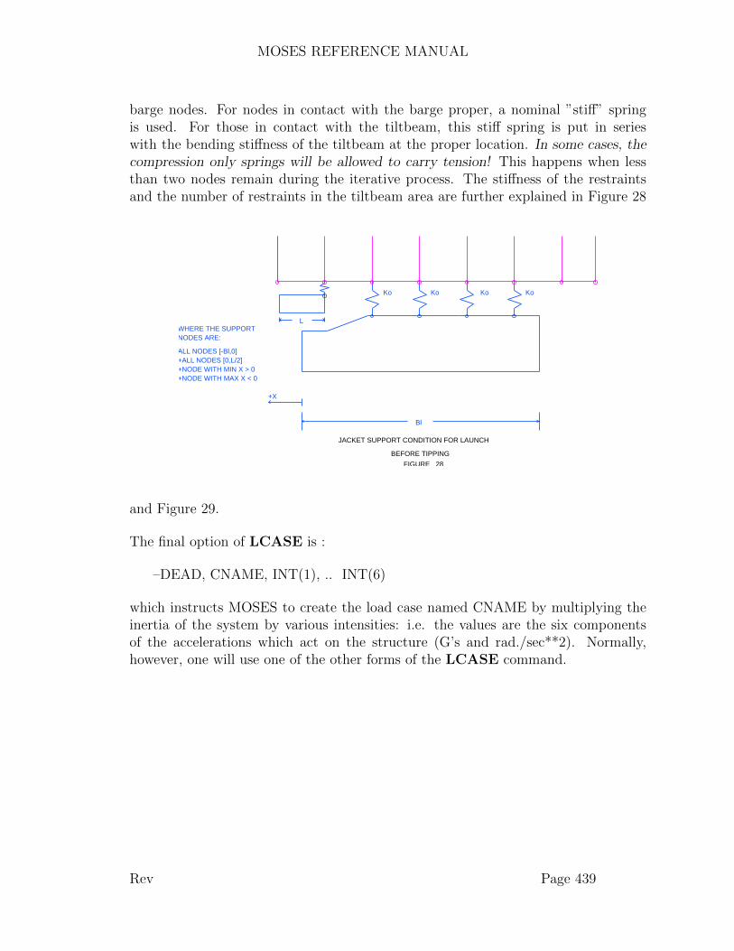
MOSES REFERENCE MANUAL
barge nodes. For nodes in contact with the barge proper, a nominal ”stiff” springis used. For those in contact with the tiltbeam, this stiff spring is put in serieswith the bending stiffness of the tiltbeam at the proper location. In some cases, thecompression only springs will be allowed to carry tension! This happens when lessthan two nodes remain during the iterative process. The stiffness of the restraintsand the number of restraints in the tiltbeam area are further explained in Figure 28
JACKET SUPPORT CONDITION FOR LAUNCH
BEFORE TIPPING
FIGURE 28
WHERE THE SUPPORTNODES ARE:
ALL NODES [-Bl,0]+ALL NODES [0,L/2]+NODE WITH MIN X > 0+NODE WITH MAX X < 0
Bl
+X
Ko Ko Ko Ko
L
and Figure 29.
The final option of LCASE is :
–DEAD, CNAME, INT(1), .. INT(6)
which instructs MOSES to create the load case named CNAME by multiplying theinertia of the system by various intensities: i.e. the values are the six componentsof the accelerations which act on the structure (G’s and rad./sec**2). Normally,however, one will use one of the other forms of the LCASE command.
Rev Page 439

MOSES REFERENCE MANUAL
JACKET SUPPORT CONDITION FOR LAUNCHAFTER TIPPING
FIGURE 29
1 1=
K b**3 1+
3EI Ko
K
K
K
K
b
Structural Element
Barge Node
Barge Node Nearest the Rocker Pin
Rev Page 440
MOSES REFERENCE MANUAL
XXVI.D Obtaining Applied Loads
If the goal of entering the Structural Menu was to generate a set of applied loads, oneshould first issue the appropriate LCASE commands, and then select the portion ofthe model for which he wishes to generate the loads. If the loads for the entire modelare desired, then no further action is necessary. If, however, loads on only a portionare desired, the loads generated can be limited by the commands:
S PART, PART NAME(1), PART TYPE(1), .. PART NAME(n), PART TYPE(n)S BODY, BODY NAME(1), BODY NAME(n), .....
Here, PART NAME(i) and BODY NAME(i) are the part and/or body names to beselected, and PART TYPE is the type of the part, and all can contain wild characters.When using S PART, a part will be selected only when both part name and typematch that of a PART NAME(i) and PART TYPE(i).
After the load cases and the model have been defined, one then exports the loads bysimply issuing the command:
EXP ALOAD
and MOSES will write the loads applied to the selected system to a file for useelsewhere. By default, this file will be named root.ppo. The user may overridethis name by using the proper options of the &DEVICE command. There are threebasic components to this file: the load case name, nodal loads (if present) and elementloads. A sample of this file is:
$&DIMEN –DIMEN Feet Kips$APLOADLOAD CASE TWO*2 6.4185E–16 6.4185E–16 –1.0000E+01 0.0000E+00 0.0000E+006.4185E–14*3 6.4185E–16 6.4185E–16 –1.0000E+01 0.0000E+00 0.0000E+006.4185E–14ELMAPL T ∼T *1 *2 .00 10.000.0000E+00 0.0000E+00 –3.8378E–02 0.0000E+00 0.0000E+00
0.0000E+000.0000E+00 0.0000E+00 –3.8378E–02 0.0000E+00 0.0000E+00
0.0000E+00ELMAPL T ∼T *1 *2 10.00 131.420.0000E+00 0.0000E+00 –4.2654E–02 0.0000E+00 0.0000E+00
0.0000E+000.0000E+00 0.0000E+00 –4.2654E–02 0.0000E+00 0.0000E+00
Rev Page 441

MOSES REFERENCE MANUAL
0.0000E+00ELMAPL T ∼T *1 *2 131.42 141.420.0000E+00 0.0000E+00 –3.8378E–02 0.0000E+00 0.0000E+00
0.0000E+000.0000E+00 0.0000E+00 –3.8378E–02 0.0000E+00 0.0000E+00
0.0000E+00
The first line in the file indicates the units used, and the second line is a commentline indicating the file content. The next line indicates the load case name for theapplied loads that follow. All loads are reported in the part coordinate system.
If there are nodal loads in the structure, they are next. The format of the nodal loadsstarts with the node name, followed by the forces and moments acting at the node:FX, FY, FZ, MX, MY, MZ. The nodal loads are continued for this load case untilan ELMAPL command is encountered.
Element loads have three lines per element. The first line begins with ELMAPLfollowed by the element name, the class name, the begin and end nodes, and the beginand end distance from the end of the beam over which the load acts. If the beginand end distances are equal then the load is concentrated. The next two lines definethe load distribution. For concentrated loads, the two lines are the same and eachone define the total load; i.e. one of these lines should be ignored. For distributedloads, the first line defines the load intensity at the beginning distance from the startof the beam and the second line at the end distance. There are six numbers on eachline corresponding to force intensities in the X, Y, and Z directions and momentintensities in X, Y, and Z directions. These loads are trapezoidally distributed loadsdefined by the intensity at each end and the portion of the beam over which it acts,as shown in Figure 30.
Normally, there will be more than one ELMAPL command for each element. Thesecome from a variety of sources, and there is no way to ascertain their origin. TheELMAPL commands are repeated for all the elements in the model that have loadfor this load case. The sequence of load case name, nodal loads and ELMAPLcommands is then repeated for each load case specified.
Rev Page 442

MOSES REFERENCE MANUAL
TRAPEZOIDAL ELEMENT LOADS
FIGURE 30
*A *B
FB
FA
XA
XB
Rev Page 443

MOSES REFERENCE MANUAL
XXVII. STRUCTURAL ANALYSIS & APPLIED LOADS
To perform a structural analysis or emit a set of applied structural loads, one mustenter the Structural Menu. This is accomplished by issuing the command:
STRUCTURAL, –OPTIONS
where the available option is:
–INITIALIZE
This command places the user in a sub–menu where he can define a situation andperform an analysis. If the option is selected, then this will delete all previous struc-tural results; otherwise, the results will be added to previous results so that all ofthem are available later for Structural Post–Processing. In general, there are threetypes of commands available in this menu: commands which define the load casesto be used, commands which define the portion of the system which will be used,and commands which produce the results. When the solution has been completed,one should issue END STRUCT to return to the main menu. There are no re-ports produced directly in this menu. The results that are produced are the systemdeflections and element loads, but to obtain a report of them, one must enter theStructural Post–Processing Menu.
Three general types of results can be obtained in this menu: structural analysisresults (system deflections and element internal loads), loads applied to the structure,or vibration modes. In the first two cases, both the load cases and the portion ofthe system to be considered must be defined before the commands to compute theresults are issued. With vibration modes, a single command suffices. The remainderof this discussion is applicable only to structural analysis and applied loads.
Before proceeding, however, it is best to make a distinction between load cases andload sets. A load set is either one of the intrinsic load sets that the program generates,or a user defined load set. Load sets are combined to form load cases. It is thesecases that are used to obtain the results. When emitting applied loads, or whenperforming a structural analysis, it is the load cases which will be used.
It is beneficial to think of the solution as being performed in one of four types:
• Frequency Domain,• Time snap–shots of a frequency domain,• Events during a MOSES generated process, or• At events in a user defined process.
Rev Page 444

MOSES REFERENCE MANUAL
Here, the types refer to the type of loadings which will be applied to the structure.MOSES is different from most programs in that the structural dynamics is includeddirectly in the analysis via generalized degrees of freedom. Thus, if generalized degreesof freedom are included during an analysis, the deformation inertia is automaticallyincluded when the load case is generated. The result is a true load case whichaccurately describes the static as well as the dynamic behavior. The type of solutionis controlled by the type of loads generated.
When a structural analysis has been performed, the results can again be combined inthe post–processor. If the problem is linear, combining the deflections in the post–processor or combining the loads prior to solution produce the same results. For anonlinear problem, however, this is not the case.
For the linear problem in the frequency domain, either options 1 or 2 defined aboveare available. Of these two methods, the frequency domain allows the user moreflexibility, while the time domain can offer some savings in computational effort. Thefrequency domain method must be used if one wishes to compute the cumulativefatigue damage for the system.
If one wishes to use nonlinear elements, the structural system of equations will benonlinear. In this case, the frequency domain solution method will not really yieldthe proper results since the solution will be for unit wave. Here, it is better tocombine loads to form the total load on the system prior to solution. Thus, onecannot correctly assess cumulative fatigue damage using nonlinear elements.
When the structural analysis is complete, one should issue:
END STRUCT
Rev Page 445

MOSES REFERENCE MANUAL
XXVIII. STRUCTURAL POST–PROCESSING
At the conclusion of the Structural Menu, the deflections and element loads arestored in the database. To obtain reports of these results, or any results which canbe derived from them, one must enter the Structural Post–Processing Menu. This isaccomplished by issuing the command,
STRPOST.
At this point, the commands discussed in this section become available. When oneis finished with Structural Post–Processing, he should issue:
END STRPOST
to return to the main menu.
For any of the commands in this menu which produce reports, the selection criteriadiscussed for the &REP SELECT command is operative. In fact, each of thesereport commands has as a subset of options, the options of the &REP SELECTcommand. Thus, it is a simple matter to obtain reports for a single element, or for anysubset of elements. In particular, for commands which deal with elements (beams,generalized plates, connectors, or restraints) only the following will be selected:
• The class name of the element must match the class selector defined by the last–CLASS option,• The nodes which form the vertices of the element all must match a node selector
defined by the last –NODE option, and• The element name must match the element selector defined by the last –
ELEMENT option.
A similar scheme is used for joints, and will be discussed later. In all cases, onlycases which match the last –LOAD selector defined will be considered. A commonmistake is to define a selector to limit one report and forget that it will also limit allsubsequent reports until the selector is redefined. In most cases, the answer to thequestion of why did I not get ... is answered by a forgotten selector.
There is a string function
&str pst(ACTION, –OPTION)
which gives information about the results obtained in the STRPOST Menu. HereACTION should be chosen from: E CHECK, E FATIGUE, E LOADS, E STRESS,J CHECK, J FATIGUE, C CHECK, C LOADS, C FOUNDATION, or DU-
Rev Page 446
MOSES REFERENCE MANUAL
RATION, and the only option is
–INITIALIZE.
MOSES saves a set of data about the ”worst” situation encountered for each typeof report in the STRPOST Menu. This information is initialized for all sets of dataeach time the menu is entered, or for a particular set when the –INITIALIZE optionis used. The prefix stands for the type of data to be returned: E for elements, Jfor joints, and C for connectors. The word following the is the type of commandfor which the data will be returned: CHECK for a code check, FATIGUE for CDRs,LOAD for internal loads, and STRESS for stresses.
The ACTION DURATION is different from all of the others. It returns informationabout the duration data used in computing fatigue. In particular it will return 4numbers:
• The number of spectra used to define the duration,• The length of time of the duration in days,• The length of tow in in feet or meters, and• The average speed of the tow in feet or meters per second.
The data returned for the other values of ACTION vary in detail, but in general willbe:
• The name of the element/joint which was the most severe,• The value which was most critical,• The number of things which failed,• The number of classes resized,• The load case which produced the worst value, and• The loads (six numbers) which produced the worst value.
The only ACTION which produces exactly what it says is E CHECK. The othersdiffer from the above as follows:
• E CHECK – follows the above exactly,• E FATIGUE – has only the first three values,• E LOADS – does not have number of classes resized,• E STRESS– does not have number of classes resized,• J CHECK – has neither the number of classes resized nor the six loads,• J FATIGUE – has only the first three values,• C CHECK – does not have number of classes resized,• C LOADS– does not have number of classes resized,
Rev Page 447

MOSES REFERENCE MANUAL
• C FOUNDATION– has neither the number of classes resized nor the sixloads.
Rev Page 448

MOSES REFERENCE MANUAL
XXVIII.A Post–Processing Cases
In all commands in the Structural Post–Processing Menu, one has the option tospecify precisely which cases to consider. One always has the ”basic” cases obtaineddirectly from the structural solution available, but one of the more powerful capabil-ities of MOSES is the ability to combine the results of the fundamental load cases toobtain new cases for post–processing. For most situations, this capability is exercisedvia the CASES command.
As mentioned above, most of the control of post–processing cases is accomplishedwith the command:
CASES POST, –OPTIONS
where the available options are:
–DELETE, :CASE SEL(1), ........., CASE SEL(n)–COMBINE, NEWNAME, CASE(1), MULT F(1), MULT P(1) ...,–AMOD, MULT, NAME(1), ........., NAME(n)–NOMINAL, NAME, MULT–PRELOAD, NAME–TIME, ENV NAME, NEWNAME(1), T(1), .........., NEWNAME(i), T(i)–PROCESS, PRC NAME–MEAN, MLCNAME–FATIGUE, DURATION NAME, TOTTIME, TOW VEL–SPECTRA, ENV NAME(1), ............., ENV NAME(i)
If one has defined some cases which he no longer needs, he can delete them by usingthe option –DELETE, which will delete all cases which match any of the selectorsCASE SEL(i).
The –COMBINE option is used to define a simple linear combination of previouslydefined cases (either fundamental or combinations themselves). Here NEWNAME isthe name the user wishes to give to this combination, CASE(i) is the name of thecases to be combined, and MULT F(i) and MULT P(i) are the multiplier for this casefor loads and pressure respectively. One really should not have two multipliers here,but some codes require multiplying the static loads by a factor. If one also multipliesthe pressures by the same factor, one gets unreasonable code pressure checks. IfMULT P is omitted, then it is set to the value of MULT F.
Some codes allow one to employ an ”allowable stress modifier”. This is a numberwhich is multiplied by the allowable stress in the computation of a code check. If theuser takes no action, these factors are set to 1. To alter these multipliers, one should
Rev Page 449

MOSES REFERENCE MANUAL
use the –AMOD option. Here, MULT is the new allowable stress modifier for caseswhich match any of the names NAME(i) and it can contain wild characters.
The allowable stress modifiers operate on ”cases”, either load cases or combine cases.They do not operate on the constituents of a combine. Thus, suppose one issues thefollowing:
CASES –AMOD 1.3 @CASES –COMBINE DOG CAT .5 BIRD .5
Since the combine case, DOG, was defined after the definition of the allowable stressmodifiers, a default modifier will be assigned. If one wishes DOG to have a differentmodifier, he must either issue another CASES –AMOD command, or define DOGbefore the –AMOD.
The –NOMINAL and –PRELOAD options define load cases and multiplier to beconsidered as the nominal and pre–load cases during a foundation code check. Theyplay the same role here as the –SET STATE option on &CONNECTOR play for aProcess Post–Processing FOUNDATION check. If either of these are not defined thevalues defined via &CONNECTOR will be used.
The –TIME option is used to produce a time domain ”snap–shot” from resultsobtained via a frequency domain structural solution. Here, ENV NAME is a seastatename which has been previously defined on an &ENV command, and NEWNAME(i)is the name given to the snapshot of the system at time T(i).
All of the other options deal with converting response operator solutions into some-thing more meaningful. MOSES associates a process name with each set of responseoperator loads cases. The –PROCESS option tells MOSES to use the response op-erators associated with process PRC NAME for all options which follow. Normally,one wishes to combine the response operators with the mean to obtain the results.Without any other action, MOSES will use the ”frequency mean” load case for thisprocess in the combination. Use of the –MEAN option instructs the program to usethe case MLCNAME instead of FRQMEAN(i) for all cases defined after the –MEANoption is encountered until a new –MEAN is encountered.
The –FATIGUE option can be used to alter the total time of exposure to a givenenvironment or the process to which it is applied. If this option is used, then wheneverthe duration DURATION NAME is used to compute fatigue, the actual exposure fora given component will be WTIME * TOTTIME / SUMTIME where TOTTIME(days) is that specified with the option, WTIME is the time specified when thecomponent was defined, and SUMTIME is the sum of WTIME(i) for the duration.If TOW VEL is specified, the length of the tow will be computed as the tow velocity
Rev Page 450
MOSES REFERENCE MANUAL
times the duration of the tow, where TOW VEL is in ft/sec or m/sec, and theduration of the tow is determined by summing the durations. When this option isused, the process associated with the duration is also changed to be the one specifiedby the preceding –PROCESS option.
The –SPECTRA option allows one to combine the frequency domain results toobtain spectral ones. Here, ENV NAME(i) are the names of environments which havebeen previously defined via &ENV commands or in the &DATA Menu. The casesdefined by this option will have the same names as the environments. These caseswill be formed as follows: First, the RMS of each force or deflection will be computedbased on the spectrum. The statistic selected by the –PROBABILITY option onthe &ENV command will then be computed. Finally, if the –USE MEAN optionwas selected when the environment was defined, the statistical result will be added tothe mean using the sign of the mean. In other words, the mean and the deviation willbe combined by adding the absolute value of the two quantities and using the signof the mean. Here, the mean is either the appropriate FRQMEAN or MLCNAME.
Rev Page 451
MOSES REFERENCE MANUAL
XXVIII.B Post–Processing & Pictures
Whenever one computes joint or element code checks or fatigue, or beam loads thelast values computed will be stored for use with pictures. Storing only a single valueis in keeping with the philosophy of checking all cases and using the maximum tosize the structure.
With animations, however, we have a different problem. Here we may want to lookat the deflections of the structure or at code checks as a function of time. Beforeyou can do this, you must have load cases that are snapshots at times during a timedomain simulation. If so, then you must tell MOSES to store the results so that youcan use them for pictures. One does this with the option
–FOR ANIMATION
on the Post–Processing command: commands:
BEAM POST CODE CHECKJOINT POST CODE CHECKJOINT POST DISPLACEMENTS
If you use this option, then
• no output of the results will be generated.• Results will be generated only for the current process. If you have more than
one process, then you need to generate the data for each process; i.e. use&DESCRIBE PROCESS to change the current process.• Once the data has been generated, it will be used in place of the ”system wide”
data for all events greater than 0.• If you define a combination case, then it will inherit the time association of the
first member of the combination.• If you have a combination case generated with the –TIME option, then it will
have the event behavior of the time specified. It will not, however, be usefulunless you use the FR 2TIME to associate a process with these events.
Perhaps it is good to look at some examples. Suppose that you have a time domainsimulation and that you generated load cases with:
&loop t 1 1000lcase –process %t &string(o number T0000)
&endloop
Now, suppose that you wanted to look at the deflections as a function of time. You
Rev Page 452

MOSES REFERENCE MANUAL
can do this with
strpostjoint deflection –load t@
end&picture iso –events 0 1000 –deflect 200 only –movie
Of course, once the deflections are associated with the events the making of thepicture is the same as with any animation.
Now, suppose you have a combination case (suppose you are doing an LRFD codecheck, etc.) Then
&loop t 1 1000&set num = &string(o number 0000)cases –combine %(c)%num %(t) 1 some –1
&endloop
will have a time association while
&loop t 1 1000&set num = &string(o number 0000)cases –combine %(c)%num some –1 %(t) 1
&endloop
will not.
Rev Page 453
MOSES REFERENCE MANUAL
XXVIII.C Post–Processing Modes
Structural Post–Processing results for modes are obtained with the command:
MODES POST, TYPE(1), ...., TYPE(i) –OPTIONS
where TYPE(i) must be chosen from VALUES or VECTOR. and the availableoptions are:
–LOAD, :LSEL–NODE, :NODE SEL
With modes, the ”load cases” are the names M00000001, M00000002, etc. where1 designates the first mode, 2 the second mode, etc. The –LOAD option can beused to select modes based on this nomenclature. If TYPE is VALUES, then theeigenvalues (natural frequencies) for the selected modes will be reported. If TYPE isVECTOR then the eigenvectors (normal modes) for each node selected by –NODE:NODE SEL will be reported.
With a TYPE of VECTOR, the command works the same way the joint deflectionsdo. In particular, one can issue &PICTURE –TYPE STRUCT immediately after thecommand to plot the mode shape.
Rev Page 454
MOSES REFERENCE MANUAL
XXVIII.D Post–Processing Connectors & Restraints
To obtain post–processing results for restraints and connectors, one should issue thecommand:
RESTRAINT POST, TYPE(1), ...., TYPE(i) –OPTIONS
where TYPE(i) must be chosen from ENVELOPE, LOADS FOUNDATION, orPILE CHECK, and the available options are:
–CLASS, :CLS SEL–NODE, :NODE SEL(1), :NODE SEL(2), :NODE SEL(3), :NODE SEL(4)–ELEMENT, :ELE SEL–LOAD, :LSEL–DETAIL–STANDARD, L(1), T(1), ..... L(n), T(n)–SUMMARY, L(1), T(1), ..... L(n), T(n)
Here, one will only receive results for elements which match the selectors defined withthe –CLASS, –NODE, and –ELEMENT options as described previously and forcases which match :LSEL which is defined with the –LOAD option. If no values aregiven for TYPE(i), then results for all TYPEs will be produced.
With a TYPE of ENVELOPE, the maximum and minimum restraint loads aresummarized for all selected load cases and the –DETAIL, –STANDARD, and–SUMMARY options are ignored.
A TYPE of LOADS will yield a report of the loads acting in the elements whichrestrain and connect the system. A TYPE of PILE CHECK will yield an APIcode check of any piles used in the solution, and a TYPE of FOUNDATION willproduce a ”foundation check”. This check is the same as the FOUNDATION checkin the Process Post–Processing menu. The only difference is that here the Nominaland Pre–load cases are those defined with the –NOMINAL and –PRELOAD optionsof the CASES command. If these are not defined, then the values defined with the&CONNECTOR command will be used.
The extent of the reports which will be produced is controlled by which of the reporttypes were –DETAIL, –STANDARD, or –SUMMARY was selected and thereport limits. With a –STANDARD or –SUMMARY report, L(i) and T(i) areused to specify a range of unity ratios for which a given report will be printed. Onecan specify as many ranges as he desires, or he can omit all data following the option.If no ranges are specified, one report for all ranges of unity ratio will be printed. Anoption of –STANDARD will result in a report of the results for the maximum unity
Rev Page 455

MOSES REFERENCE MANUAL
ratio over all selected load cases for each member selected. If one specifies an option of–SUMMARY, this report will be reduced to the results for only the selected elementin each class which has the greatest unity ratio. Finally, if one specifies –DETAIL asan option, the original report will be expanded to include checks of all members forall selected load cases at all load points. Notice that –DETAIL, –STANDARD,and –SUMMARY may all be used on the same command to produce reports of allthree types. Also, if no options are specified, then a default of –STANDARD isassumed.
Rev Page 456
MOSES REFERENCE MANUAL
XXVIII.E Bending Moments and Shears
Bending moments and shears are somewhat different from the other commands inthe Structural Post–Processing Menu in that one is placed in the Disposition Menuso that the results can be graphed, viewed, or saved. To obtain these results, oneshould issue the command:
BMOM SHR, SELE DATA –OPTIONS
here SELE DATA is the data that selects the beams to be processed and is either:
BMOM SHR, ELE(1), ELE(2), ... ... ELE(n–1) –OPTIONS
or
BMOM SHR, *NODE(1), *NODE(2), ... *NODE(n) –OPTIONS
where the only option is:
–LOAD, :LSEL
With the first form of this command, one defines a string of beams which lie in a lineby specifying their names, ELE(i). With the second, the elements are defined by theelements connecting a string of nodes. With this form of the command, the stringfunction &NODE(N 2NODES *NODE(1), *NODE(n)) can be used here to find theintermediate nodes; i.e. an alternative to the above is:
BMOM SHR, &NODE(N 2NODES *NODE(1), *NODE(n)) –OPTIONS
Please notice that SP BEAMS are not real ”elements” so that for this type of element,the first form of the command must be used. When either of these commands isissued, MOSES will find the beams connecting the nodes and store the elementforces for each stress point of each beam according to the distance of the stress pointfrom the first node of ELE(1) or *NODE(1) depending upon how the command wasissued. The loads for up to 10 loads cases selected by :LSEL will be considered. Afterthe data has been obtained, the user is placed in the Disposition Menu to dispose ofit as he sees fit.
Another command which deals with moments and shears is:
Rev Page 457

MOSES REFERENCE MANUAL
COUNT FM POST, ELE(1), ELE(2), ... ... ELE(n–1) –OPTIONS
or
COUNT FM POST, *NODE(1), *NODE(2), ... *NODE(n) –OPTIONS
where the options are:
–FM BINS, F(1), M(1), ....., F(n), M(n)–DURATION, :DURATION SEL
which allows one to have the number of cycles of the bending moments and shears bro-ken down into ”bins”. The beams are selected for processing as with the BMOM SHRcommand. The –FM BINS option defines the values for force, F(i) (bforce), and mo-ment, M(i) (bforce–blength) which are used to delimit the bins, and the –DURATIONoption selects the durations which will be used to count the cycles.
Rev Page 458

MOSES REFERENCE MANUAL
XXVIII.F Force Response Operators
Response operators of the forces in beams and connectors are obtained with thecommand:
F RAO POST, –OPTIONS
and the available options are:
–CLASS, :CLS SEL–NODE, :NODE SEL(1), :NODE SEL(2), :NODE SEL(3), :NODE SEL(4)–ELEMENT, :ELE SEL–DETAIL–STANDARD, L(1), T(1), ..... L(n), T(n)–SUMMARY, L(1), T(1), ..... L(n), T(n)–REPORT, YES/NO–FILE, YES/NO
Here, one will only receive RAOs for elements which match the selectors defined withthe –CLASS, –NODE, and –ELEMENT options as described previously.
The extent of the reports which will be produced is controlled by which of the threereport types –DETAIL, –STANDARD or –SUMMARY were selected and thereport limits. With a –STANDARD or –SUMMARY report, L(i) and T(i) areused to specify a range of values for which a given report will be printed. The valueused for determining the range is the axial load. One can specify as many ranges ashe desires, or he can omit all data following the option. If no ranges are specified, onereport for all ranges of axial load will be printed. An option of –STANDARD willresult in a report of the RAOs for the maximum axial force over all selected periodsand headings for each member selected. If one specifies an option of –SUMMARY,this report will be reduced to the RAOs for only the selected element in each classwhich has the greatest axial force. Finally, if one specifies –DETAIL as an option,the original report will be expanded to include checks of all members for all periodsand headings at all load points. Notice that –DETAIL, –STANDARD, and –SUMMARY may all be used on the same command to produce reports of all threetypes. Also, if no options are specified, then a default of –STANDARD is assumed.
The options –REPORT and –FILE are used to control whether or not the RAOsare written to a post–processing file, or the standard output file. The default is towrite them only to the output file. If –FILE YES is specified, then the RAOs willbe written to both places. If –FILE YES –REPORT NO is specified, then theRAOs will only be written to the post–processing file.
Rev Page 459
MOSES REFERENCE MANUAL
XXVIII.G Post–Processing Beams
Structural Post–Processing results for beams are obtained with the command:
BEAM POST, TYPE(1), ...., TYPE(i) –OPTIONS
where TYPE(i) must be chosen from LOADS, CODE CHECK, H COLLAPSE,ENVELOPE, STRESS, COUNT, NT FATIGUE, or FATIGUE, and the avail-able options are:
–CLASS, :CLS SEL–NODE, :NODE SEL(1), :NODE SEL(2), :NODE SEL(3), :NODE SEL(4)–ELEMENT, :ELE SEL–LOAD, :LSEL–DURATION, :DURATION SEL–CODE, TYPE, CCAT–STANDARD, L(1), T(1), ..... L(n), T(n)–SUMMARY, L(1), T(1), ..... L(n), T(n)–DETAIL–DOF SEL, DOF–REPORT, YES/NO–FILE, YES/NO–B LOAD, YES/NO–EQUIVALENT, YES/NO–RESIZE, CONT–COSTS, STCOST, RCOST–UP CLASS, YES/NO–S BINS, S(1), S(2), ......, S(n)–SLA COEFFICIENT, S COE–SLA DAF, S DAF–SLA CDAMP, S CDAMP–SLA FIXITY, S FIXITY–SLA MULTIPLIER S VEL(1), S MUL(1), ... S VEL(n), S MUL(n)
Here, one will only receive results for elements which match the selectors defined withthe –CLASS, –NODE, and –ELEMENT options as described previously and forcases which match :LSEL which is defined with the –LOAD option. For COUNT,NT FATIGUE or FATIGUE, all durations which match :DURATION SEL de-fined via the –DURATION option will be considered. If no values are given forTYPE(i), then results for all TYPEs will be produced.
Here, a TYPE of
Rev Page 460
MOSES REFERENCE MANUAL
• LOADS will produce the internal element loads,• CODE CHECK will produce a report of the elements checked against the
code specified by the –CODE option,• H COLLAPSE will produce an API hydrostatic collapse check,• ENVELOPE will produce an envelope of beam stresses or loads,• STRESS will produce the stresses at ”stress points” for each longitudinal
location on the beam,• COUNT will produce the number of cycles of the stresses in ”bins”, and• NT FATIGUE or FATIGUE will produce fatigue results. Here, NT FATIGUE
will consider only sections of beams which are not part of tubular joints andFATIGUE will consider all beams.
With the exception of a TYPE of COUNT, the extent of the reports which willbe produced is controlled by which of the three report types were selected and thereport limits. With a –STANDARD or –SUMMARY report, L(i) and T(i) areused to specify a range of values for which a given report will be printed. Remember,the beams for which results are computed is already restricted by the –CLASS, –NODE, and –ELEMENT selectors, and the load cases by the –LOAD selectors.Thus, here we are talking about restricting what is reported out of what is computed.The easiest of these to describe is –DETAIL. Here, all the results are printed. With –STANDARD, only the result with the greatest ”value” is a candidate for reporting,and it will only be reported if the value is between the report limits specified for thatreport. What is meant by ”value” depends on type and will be described later. Witha report option of –SUMMARY, only the result with the greatest value for a classis a candidate for reporting. One can specify as many ranges as he desires, or hecan omit all data following the option. If no ranges are specified, one report for allranges of value will be printed. An option of –STANDARD will result in a reportof the results for the maximum ”value” over all selected load cases for each memberselected. If one specifies an option of –SUMMARY, this report will be reduced tothe results for only the selected element in each class which has the greatest ”value”.Notice that –DETAIL, –STANDARD, and –SUMMARY may all be used onthe same command to produce reports of all three types. Also, if no options arespecified, then a default of –STANDARD is assumed. For a type of STRESS, thereporting criteria is the Von Mises stress divided by the yield stress, for a type ofFATIGUE, the value is the CDR, and for all others except LOADS it is the codeunity value.
For a TYPE of LOADS, the value used for determining the range is the absolutevalue of DOF in bforce or bforce–blength units. For this type, The –DOF SELoption is used to specify the degree of freedom to be used as the reporting criteria.With this option, DOF is selected from the list: FX, FY, FZ, MX, MY, MZ,SHEAR or MOMENT. Only one value may be selected, and the default value is
Rev Page 461
MOSES REFERENCE MANUAL
FX, axial. The value for DOF determines which quantity of the beam is used asthe criteria for selecting the load case to report. When using the –STANDARD or–SUMMARY options, only the load case providing the highest absolute value ofDOF is reported. The options –REPORT and –FILE operate only with a TYPEof LOADS. These options are used to control whether or not the results are writtento a post–processing file, or the standard output file. The default is to write themonly to the output file. If –FILE YES is specified, then the results will be writtento both places. If –FILE YES –REPORT NO is specified, then the results willbe written to the post–processing file only.
The options –CODE, –EQUIVALENT, –RESIZE, –COSTS, –UP CLASS,and –B LOAD are applicable only to a TYPE of CODE CHECK. The type ofcode which will be used depends upon the last –CODE option. Here, TYPE maybe either AISC, API, NORSOK, or ISO. The value CCAT defines the class ofcheck for AISC or API type checks. It should be omitted for ISO or NORSOKtype checks and it must be either WS or LRFD for AISC or API checks. If it isomitted for these checks, WS will be assumed. If one wishes to use an LRFD check,it is his responsibility to build load cases which include the proper multipliers. Thisoption is remembered between BEAM code checks and JOINT checks. Thus, if onehas previously used the –CODE option he need not be re–issued. If one is checkingNORSOK or ISO codes, non tube beams will be checked using EUROCODE 3. NoNational Annex changes are considered and class 4 sections are treated as failures.
None of the codes are clear in how to treat non–prismatic members with respectto buckling. If one uses the –EQUIVALENT option with NO, then each sectionis checked using a slenderness based on the geometrical properties of that section,the ”k” factor, and the length. If, however, this option is used with YES, then theslenderness of each section will be based on an estimate of the true buckling loadof the element; i.e. a Raleigh Quotient will be used to compute the Euler criticalload in the element and then a slenderness (and hence a radius of gyration) will becomputed for each section which when combined with the standard formulae yieldthe estimated Euler buckling load.
The –RESIZE option directs MOSES to resize the selected classes so that eachmember will have a unity ratio less than one for the load cases considered. If CONTis UP and a class has a unity ratio less than one, no change in the class will bemade. If either the unity ratio is greater than one or CONT is UPDOWN, the classwill be resized. The manner in which MOSES picks a new member depends uponthe table selector specified on the –RDES option for the class definition command.The shapes selected by the selector are assigned a cost based on the two unit costsdefined via the –COSTS option. Here, STCOST is the cost of steel in monetaryunits per bforce, and RCOST is the corresponding cost of adding a single hydrostatic
Rev Page 462

MOSES REFERENCE MANUAL
ring. The selected shapes are then tried in order of increasing cost until a workableshape is found. If –UP CLASS is specified with YES/NO equal YES, then thenew sizes will be stored in the database. Otherwise, the original sizes will remain.If –B LOAD is specified with YES/NO equal to YES, a third line will be addedto the code check output. This line contains the loads which produced the reportedstresses.
For a TYPE of ENVELOPE, the maximum and minimum internal element loadsare summarized for all selected load cases. This is quite useful in understanding thenature of loadings in the beam elements of a structure. If –DETAIL is specifiedas an option, the envelope of loads is reported at all load points. With an optionof –STANDARD, the maximum and minimum values are reported once, for anylocation on the beam.
The –S BINS option is applicable only to a type of COUNT. It is used to define aset of ”bins” by stress range to accumulate the cycle data. Here, S(1) (ksi or mpa)marks the ”top” of the first bin, S(2) the top of the second bin, etc. The stresseswhich are accumulated include the stress concentration factor.
The options –SLA COEFFICIENT, –SLA DAF, –SLA CDAMP, –SLA FIXITY,or –SLA MULTIPLIER are applicable only to a TYPE of FATIGUE. They de-fine the parameters used in frequency domain slamming fatigue are are discussedin the section on Beam Fatigue Due to Slamming. If you do not want to considerslamming, you should use
–SLA COEFFICIENT 0.
Also with FATIGUE, the meaning of –DETAIL, –STANDARD, and –SUMMARYis a bit different. –DETAIL is ignored. For –STANDARD, one receives the totalCDRs for all computed points where the maximum of the CDRs lie between L(i) andT(i). Finally, for –SUMMARY, one only receives a report of the maximum CDRfor all of the computed points which lie in the specified range.
Rev Page 463
MOSES REFERENCE MANUAL
XXVIII.H Post–Processing Generalized Plates
Structural Post–Processing results for generalized plates are obtained with the com-mand:
PLATE POST, TYPE(1), ...., TYPE(i) –OPTIONS
where TYPE(i) must be chosen from STRESS, LOADS, FATIGUE, or COUNT,and the available options are:
–CLASS, :CLS SEL–NODE, :NODE SEL(1), :NODE SEL(2), :NODE SEL(3), :NODE SEL(4)–ELEMENT, :ELE SEL–LOAD, :LSEL–DURATION, :DURATION SEL–DETAIL–STANDARD, L(1), T(1), ..... L(n), T(n)–SUMMARY, L(1), T(1), ..... L(n), T(n)–REPORT, YES/NO–FILE, YES/NO–S BINS, S(1), S(2), ......, S(n)–CDR VONMISES, FLAG
Here, one will only receive results for elements which match the selectors defined withthe –CLASS, –NODE, and –ELEMENT options as described previously, and forcases which match :LSEL which is defined with the –LOAD option. For FATIGUE,all durations which match :DURATION SEL defined via the –DURATION optionwill be considered. If no values are given for TYPE(i), then results for all TYPEswill be produced.
Here, a TYPE of STRESS will produce the average stress in the element, LOADSwill produce the membrane tractions acting on the faces of the element and the aver-age bending stresses, FATIGUE will produce spectral fatigue results, and COUNTwill produce the number of cycles of the stresses in ”bins”. With the exception ofCOUNT, the extent of the reports which will be produced is controlled by which ofthe three report types –DETAIL, –STANDARD or –SUMMARY were selectedand the report limits. With a –STANDARD ob –SUMMARY report, L(i) andT(i) are used to specify a range of values for which a given report will be printed. Thevalue used for determining the range is the Von Mises stress divided by yield stressexcept for FATIGUE where the value is the CDR. One can specify as many ranges ashe desires, or he can omit all data following the option. If no ranges are specified, onereport for all ranges of value will be printed. An option of –STANDARD will resultin a report of the results for the maximum unity ratio over all selected load cases for
Rev Page 464
MOSES REFERENCE MANUAL
each member selected. If one specifies an option of –SUMMARY, this report willbe reduced to the results for only the selected element in each class which has thegreatest unity ratio. Finally, if one specifies –DETAIL as an option, the originalreport will be expanded to include checks of all members for all selected load cases atall load points. Notice that –DETAIL, –STANDARD, and –SUMMARY mayall be used on the same command to produce reports of all three types. If no optionsare specified, then a default of –STANDARD is assumed.
The options –REPORT and –FILE operate only with a TYPE of LOADS. Theseoptions are used to control whether or not the results are written to a post–processingfile, or the standard output file. The default is to write them only to the output file.If –FILE YES is specified, then the results will be written to both places. If –FILE YES –REPORT NO is specified, then the results will only be written tothe post–processing file.
The last options are applicable only to a TYPE of FATIGUE or COUNT. Thesets of duration data which will be used are those which match the selector :DU-RATION SEL defined with the –DURATION option. The –S BINS option isapplicable only to a type of COUNT. It is used to define a set of ”bins” by stressrange to accumulate the cycle data. Here, S(1) (ksi or mpa) marks the ”top” of thefirst bin, S(2) the top of the second bin, etc. The stresses which are accumulatedinclude the stress concentration factor. If stress used in computing the CDR dependson the value of FLAG following the –CDR VONMISES option. If it is YES theVon Mises stress will be used. If it is NO then the principle stresses will be used. Alsowith FATIGUE, the meaning of –DETAIL, –STANDARD, and –SUMMARYis a bit different. –DETAIL is ignored. For –STANDARD, one receives the totalCDRs for all computed points where the maximum of the CDRs lie between L(i) andT(i).
Rev Page 465

MOSES REFERENCE MANUAL
XXVIII.I Post–Processing Joints
Structural Post–Processing results for joints are obtained with the command:
JOINT POST, TYPE(1), ...., TYPE(i) –OPTIONS
where TYPE(i) must be chosen from DISPLACEMENT, CODE CHECK, S FATIGUE,CRUSH, COUNT, or FATIGUE, and the available options are:
–NODE, :NODE SEL(1), :NODE SEL(2), :NODE SEL(3), :NODE SEL(4)–ELEMENT, :ELE SEL–LOAD, :LSEL–STANDARD, L(1), T(1), ..... L(n), T(n)–SUMMARY, L(1), T(1), ..... L(n), T(n)–DETAIL–REPORT, YES/NO–FILE, YES/NO–LOCAL, YES/NO–CLASS, :CLS SEL–CODE, TYPE, CCAT, EDITION–SN, CURVE, TYPE, S(1), N(1), ..... S(n), N(n)–THICK SN, TO, POWER, MAXCOR, YES/NO–LIFE, DLIFE–WL RANGE, –ELEV, +ELEV–DURATION, :DURATION SEL–S BINS, S(1), S(2), ......, S(n)–CSRV JFAT, YES/NO–CLS MEAN, YES/NO
Here, joints which match :NODE SEL(1) will be considered. Further, if the class ofthe chord does not match :CLS SEL, the joint will not be considered. Only braceswith end nodes which match both :NODE SEL(1) and :NODE SEL(2), names whichmatch :ELE SEL, and classes which match :CLS SEL will be considered. Results willonly be considered for cases which match :LSEL which is defined with the –LOADoption. For FATIGUE, all durations which match :DURATION SEL defined viathe –DURATION option will be considered. If no values are given for TYPE(i),then results for all TYPEs will be produced.
Here, a TYPE of
• DISPLACEMENT will produce the deflections of the selected joints,• CODE CHECK will produce a report of the joint checked against API–
RP2A,
Rev Page 466
MOSES REFERENCE MANUAL
• S FATIGUE will produce a report of the API–RP2A simplified fatigue check,• CRUSH will produce a report of the crush unities based on effective closed
ring analysis,• COUNT will produce the number of cycles of the stresses in ”bins”, and finally,• FATIGUE will produce CDRs computed using a stochastic fatigue approach.
The extent of the reports except for DISPLACEMENT and COUNT is controlledby which of the three report types were selected and the report limits. With a –STANDARD or –SUMMARY report, L(i) and T(i) are used to specify a range ofcode unity values for which a given report will be printed. For a TYPE of FATIGUE,the value is the CDR, and for all others it is the code unity value. One can specifyas many ranges as he desires, or he can omit all data following the option. If noranges are specified, one report for all ranges of value will be printed. An option of–STANDARD will result in a report of the results for the maximum unity ratioover all selected load cases for each member selected. If one specifies an option of –SUMMARY, this report will be reduced to the results for only the selected elementin each class which has the greatest unity ratio. Finally, if one specifies –DETAIL asan option, the original report will be expanded to include checks of all members forall selected load cases at all load points. Notice that –DETAIL, –STANDARD,and –SUMMARY may all be used on the same command to produce reports of allthree types. If no options are specified, –STANDARD is assumed.
For a TYPE of DISPLACEMENT, three additional options are available: –REPORT,–FILE, and –LOCAL. The first two of these options are used to control whether ornot the results are written to a post–processing file, or to the standard output file.The default is to write them only to the output file. If –FILE YES is specified, thenthe results will be written to both places. If –FILE YES –REPORT NO is speci-fied, then the results will only be written to the post–processing file. By default, thedisplacements are reported in the body part system. If one uses the option –LOCALNO, then the displacements will be reported in the ”current” global system. Notice,since the structural results can come from many different processes at many differentevents, the current global system may not be a good system in which to view thedeflections produced at events with a different configuration.
The type of unity ratio which will be computed for types of CRUSH and CODE CHECKdepends upon the last –CODE option. The type of code which will be used dependsupon the last –CODE option. Here, TYPE may be either AISC, API, NOR-SOK, or ISO. The value CCAT defines the class of check for AISC or API typechecks. It should be omitted for ISO or NORSOK type checks and it must beeither WS or LRFD for AISC or API checks. If it is omitted for these checks,WS will be assumed. If one wishes to use an LRFD check, it is his responsibilityto build load cases which include the proper multipliers. This option is remembered
Rev Page 467
MOSES REFERENCE MANUAL
between BEAM code checks and JOINT checks. Thus, if one has previously used the–CODE option he need not be re–issued. EDITION defines the edition of RP2Awhich will be used checked for the check. If it is OLD, then the first supplement ofthe 21st edition will be used otherwise the ”new” method will be used. If one wishesto use an LRFD check, it is his responsibility to build load cases which include theproper multipliers.
For a type of CRUSH the results computed consist of the force and moment in thechord due to the braces, stresses in the chord as a function of angle around the chord,and a unity ratio. The unity ratio is the larger of the stress unity based on an allowableof .6Fy and the shear unity based on an allowable of .4Fy. The stress reported isthe stress which produced the unity ratio. This angle is measured clockwise fromthe first brace. For the options –STANDARD and –SUMMARY only the resultsat the angle which corresponds to the highest unity check are reported, while if theoption –DETAIL is selected, one will receive results for all 36 angles around thejoint. The stresses are computed by superimposing stresses due to each brace loadand using the formulae for circular rings in Roark’s Formulas for Stress and Strain,Sixth Edition. Here, the length of the ring is taken to be the ”effective length” of thejoint according to API–RP2A. For each brace, two cases are added: first, a uniformload distributed over a segment of the chord equal the brace diameter, and second ashear around the circumference of the chord.
The –SN, –F STRESS, and –THICK SN options are used to define the SN curvewhich will be used in computing the cumulative damage ratios, and are discussedin detail in the section on Defining and Associating SN curves. The two options–LIFE and –WL RANGE are applicable only to a TYPE of S FATIGUE. Here,DLIFE is the design life, which must be either 20 or 40. The two parameters –ELEVand +ELEV define the distances below and above the water surface between whichmembers will be considered to be ”waterline” members. –ELEV should be a negativenumber and +ELEV should be a positive one.
The –DURATION option is applicable only to types of FATIGUE and COUNTand tells MOSES to use only the sets of duration data which match :DURATION SEL.The –S BINS option is applicable only to a type of COUNT. It is used to define aset of ”bins” by stress range to accumulate the cycle data. Here, S(1) (ksi or mpa)marks the ”top” of the first bin, S(2) the top of the second bin, etc. The stresseswhich are accumulated include the stress concentration factor, but not any stressconcentration due to an SN curve.
The final options are applicable only to a TYPE of FATIGUE. Also with FA-TIGUE, the meaning of –DETAIL, –STANDARD, and –SUMMARY is a bitdifferent. –DETAIL is ignored. For –STANDARD, one receives the total CDRsfor all computed points where the maximum of the CDRs lie between L(i) and T(i).
Rev Page 468

MOSES REFERENCE MANUAL
Finally, for –SUMMARY, one only receives a report of the maximum CDR for allof the computed points which lie in the specified range. The –CSRV JFAT optioncontrols the action taken with the brace/chord SCFs. MOSES computes CDRs ateight points around the intersection of the brace with the chord. If YES/NO is NO,both the brace and chord side are considered, and sixteen CDRs will be computed.If, however, YES/NO is YES, then the maximum of the two SCF values is taken anda CDR is computed for these values of SCF at the eight points. A value of YES willyield slightly conservative values and significantly reduce the computational effort.The –CLS MEAN option controls the manner in which the joint is classified if theprevious option is not used. IF YES/NO is YES, then the joint will be classifiedusing the frequency mean load case; otherwise, MOSES will compute a new jointclassification (and hence SCF) for each force response operator.
Rev Page 469

MOSES REFERENCE MANUAL
Index∼, 137, 166, 211, 214, 224, 226, 230, 231,
236, 238, 239*, 137, 203, 205–, 74.AND., 76.EQ., 76.GE., 76.GT., 76.LE., 76.LT., 76.NE., 76.NOT., 76.OR., 76:, 40#, 187, 188, 251, 268#AMASS, 268#AREA, 270#BUOY, 269#DRAG, 269#ELAT, 250#PLATE, 270#TABLE, 271#TANAKA, 272#TANKER, 274#TUBE, 271#WEIGHT, 268&APPLY, 188&BODY(, 195&BUILDG, 51&CHANNEL, 31&CLASS(, 213&CMP BAL, 302&COLOR, 25&COMPARTMENT, 298&COMPARTMENT(, 296&CONNECTOR, 321&CONNECTOR(, 309&CONVERT, 141&CTYPE, 37
&CUTYPE, 37&DATA A TABLE, 272&DATA CONVOLUTION, 153&DATA CURVES, 154&DATA DURATION, 169&DATA ENVIRONMENT, 166&DATA SHAPES, 222&DATA SOIL, 224&DEFAULT, 144, 187&DEFINE, 98&DESCRIBE ACTIVITY, 201&DESCRIBE BODY, 191&DESCRIBE COMPARTMENT, 276&DESCRIBE HOLE, 294&DESCRIBE INTEREST, 204&DESCRIBE LOAD GROUP, 265&DESCRIBE NODE NAS, 203&DESCRIBE PART, 197&DESCRIBE PIECE, 278&DESCRIBE PROCESS, 326&DESCRIBE SENSOR, 156&DESCRIBE SYSTEM, 201&DEVICE, 34&DIMEN, 22&D GENERATE, 47&ELEMENT(, 240&ELSE, 71&ELSEIF, 71&EMIT, 139&ENDIF, 71&ENDLOOP, 71&ENDMACRO, 73&END &D GENERATE, 47&ENV, 158&ENV(, 167&EOFILE, 72&EQUI, 402&ERROR, 37&EVENT STORE, 327
Rev Page 470

MOSES REFERENCE MANUAL
&EXIT, 71&EXPORT MESH, 287&EXPORT POINTS, 204&E STRING, 88&FILE, 94&FINISH, 72&FORMAT(, 76&FVGET(FUNNAM, VAR), 99&FVPUT, 99&F READ(, 94&GET(, 86&IF, 71&INFO(, 78, 94, 189&INSERT, 36&INSTATE, 198&LOADG(, 266&LOCAL, 70&LOGDEVICE, 30&LOGICAL(, 76&LOOP, 71&MACRO, 73&MENU, 92&M ACTIVE, 75&M CNAME, 75&M DELETE, 75&NAMES, 122&NAMES(, 122, 139&NEXT, 71&NUMBER(, 80&NUMVAR(, 98&PANEL(, 281&PARAMETER, 149&PART(, 198&PATH, 136&PICTURE, 55&PIECE(, 280&PI VIEW, 55&POINT(, 208&PROCESS(, 327&READY, 100&REPORT, 37&REP SELECT, 120, 173, 183
&SELECT, 40, 41&SET, 69&SLAM(, 407&STATUS, 125&STRING, 88&STRING(, 83&STYLE, 28&SUBELEMENT(, 242&SUBTITLE, 37&SUMMARY, 130&SURFACE, 288&SUSPEND, 100&S BACK, 11&TABLE, 53&TITLE, 37&TOKEN(, 85&TYPE, 37&UGX, 43&VARIABLE, 97&VARIABLE(, 97&V EXIST(, 76&V TRANSF, 210&WEIGHT, 200&str pst(, 446{
I}, 49LIST}, 50PRE}, 48TABLE}, 50U}, 49
{BPAGE,}, 49{CENTER }, 50{CONTENTS,}, 49{EJECT}, 48{EODD}, 48{FOOT,}, 48{HEAD,}, 48{INDEX,}, 49{I}, 49{LIST,}, 49{MOVE,}, 48{PART,}, 49
Rev Page 471

MOSES REFERENCE MANUAL
{PRE}, 48{RPAGNUM,}, 48{SECTION,}, 49{SKIP,}, 48{STYLE,}, 47{SUBPART,}, 49{TABLE,}, 50{U}, 49{b}, 49
ADD COLUMN, 105AGAIN, 116ALIAS, 260ANGLE, 272ARC, 45ASSEMBLY CONTROL, 319ASSEMBLY LLEG, 312ASSEMBLY PULLEY, 311ASSEMBLY T–H DEFINITION, 315ASSEMBLY WINCH, 320
BBOX, 43BEAM, 247BEAM POST, 460BEAM SUM, 131BEGIN, 411BLOCK, 288BMOM SHR, 457BODY FORCE, 419BOUNDS CONN, 352BOX, 45
C LENGTH, 426C SCALE, 101C SHIFT, 101CASES POST, 449CATEG SUM, 133CF MAGNITUDE, 427CF TOTAL, 427CFORM, 356CL D/T RESIZE, 305CL DELETE, 304CLASS SUM, 133
COLOR, 44COMPART SUM, 130CONFORCE, 427CONN DESIGN, 345CONNECTOR, 308COUNT CF, 398COUNT FM POST, 457CSYMBOL, 45CTEXT, 46CTYPE, 38CURR ARE, 272CUTYPE, 38
DELETE BLOCK, 289DEPTH, 224DESIRE VALUE, 352DIFFERENCE, 289DIMENSION, 46DLINE, 45DO REPO, 352DRAFT, 420
E MDRIFT, 379E PRESSURE, 374E TOTAL, 374ED CLASS, 212, 304ED ELEMENT, 240, 304ED POINT, 178, 203EL ACTIVE, 304EL DELETE, 304ELA DELETE, 304ELMFORCE, 424EMIT, 290END, 108, 141END &DATA, 166, 222, 224, 272END &SEL, 40END &SUMMARY, 130END &SURFACE, 288END &TABLE, 53END &UGX, 43END BLOCK, 288END DURATION, 169END FREQ RESPONSE, 381
Rev Page 472

MOSES REFERENCE MANUAL
END HYDRODYNAMICS, 370END I PRESSURE, 376END I TOTAL, 376END INPG, 167END M DRIFT, 380END MEDIT, 136END MESH, 288END PGEN, 282END PRCPOST, 417END REPO, 352END REPORT, 37END STRPOST, 446END STRUCT, 432, 433, 444, 445ENVIRONMENT, 166EQU SUM, 387EQUI H, 357EXCEPT, 41EXFORCE, 387EXP ALOAD, 441EXTREME, 110
F RAO POST, 459FAT CFORCE, 397FDELP, 376FFT, 108FIG NUM, 46FILL, 45FLOOD, 414FOUNDATION, 427FP MAP, 375FP STD, 385FPANEL, 375FPPHI, 375FR 2TIME, 385FR CFORCE, 396FR FCARGO, 393FR PANPRESS, 400FR POINT, 389FREQ RESPONSE, 381
G MDRIFT, 379G PRESSURE, 373GEN OFFS, 305
GEOMETRY, 347GOTO, 412GRID SUM, 134
H AMASS, 377H DAMP, 377H EULERA, 377H FORCE, 377H ORIGIN, 377H PERIOD, 377HOLE FLOODING, 423HORIZONTAL, 167HSTATICS, 354HYDRODYNAMICS, 370
I BEGIN, 331I CONNECTOR 4 TIE, 335I CONNECTOR PCONNECT, 335I CONNECTOR H BRACE, 335I CONNECTOR P BRACE, 335I CONNECTOR PCONNECT, 335I CONNECTOR UP SLING, 334I CONNECTOR V BRACE, 335I CONNECTOR V CAN, 336I CONNECTOR V LWAY, 336I CONNECTOR V REST, 336I CONNECTOR XY DELTA, 335I MDRIFT, 379I PRESSURE, 375I SET B SN, 330I SET C CODE, 330I SET CODE LIM, 330I SET DO MOVIE, 329I SET FAT LIM, 330I SET MARGIN, 329I SET N CODE, 330I SET N FAT, 330I SET PER APPLY, 329I SET RENDER, 329I SET SCF, 330I SET SN, 330, 331I SET T CODE, 329I SET WDEPTH, 329
Rev Page 473

MOSES REFERENCE MANUAL
I TANK, 333I TOTAL, 376INFO SEL, 41INMODEL, 135INST LAUNCH, 341INST LIFT –OPTIONS, 341INST LOADOUT, 337INST SPOST, 344INST TRANSP, 338INST UP, 343INTERSECT, 289
JOINT POST, 466
KG ALLOW, 368
LAUNCH, 408LAUP STD, 417LCASE, 436LDGFORCE, 424LG DELETE, 304LIFT, 413LINE, 45LIST BLOCK, 289LIST SEL, 41LOADG SUM, 131LWFORCE, 428
M DRIFT, 380M PAN FIX, 284MAP, 286MATRICES, 387MD MOTION, 380MEDIT, 136, 304MESH, 288MODEL IN, 332MODES, 434MODES POST, 454MOMENT, 358MOVE, 348MOVE BLOCK, 289MOVETO, 45MPY, 224MQW, 224
MTZ, 224
NAME, 40
P MIN DISTANCE, 422P TANAKA, 273PANEL, 281PCONNECT, 260PGEN, 282PICTURE, 290PILE DESIGN, 349PIPE, 317PLANE, 283PLATE, 253PLATE POST, 464PLATE SUM, 132PLOT, 115PMOTION, 391POINT SUM, 133POINTS, 421POSITION, 431PRCPOST, 417PROPULSION, 351PY, 224
QW, 224
R DETAIL, 429R ENVELOPE, 429R TANAKA, 273R VIEW, 430RANGE, 117RAO, 382RARM, 359RARM STATIC, 415REFINE, 256REFLECT BLOCK, 289REL MOTION, 421RENAME BLOCK, 290REPO, 352REPORT, 103REST, 308RESTRAINT POST, 455RESTRAINT SUM, 132
Rev Page 474

MOSES REFERENCE MANUAL
REVERSE, 281REVIEW, 415
S BODY, 441S GRID, 166S PART, 441SAVE GRAPH, 116SELECT, 40SELECT CONN, 352SENSOR, 420SET VARIABLE, 118SHOW SYS, 352SLING DESIGN, 350SP BEAM, 264SP CFORCE, 397SP FCARGO, 395SP PLATE, 264SP POINT, 391SPECTRUM, 108SRESPONSE, 383ST CFORCE, 397ST CLEARANCE, 391ST EXFORCE, 388ST FCARGO, 394ST PANPRESS, 400ST POINT, 390ST RFORCE, 398ST RSTRESS, 399STAB OK, 362, 366STABILITY, 431STATIC PROCESS, 410STATISTIC, 111STORE, 103STP STD, 417STRPOST, 169, 446STRUCTURAL, 432, 444STYLE, 44
T PRESSURE, 166TAB ADD, 89TABLE, 346TANK BAL, 423TANK CAPACITY, 355
TANK FLD, 423TDOM, 405TDOWN, 261TEXT, 46TEXT ADD, 89TIP–HOOK, 428TOWSOLVE, 435TRAJECTORY, 418TRANS CON, 261TRANSFORM, 44TUBTANK, 277TUG DCHANGE, 352TYPE, 38TZ, 224
UNION, 289USE MAC, 136USE VES, 136, 331
V EXFORCES, 374V MATRICES, 374V MDRIFT, 379VERTICAL, 167VIEW, 103VLIST, 101
WEIGHT CONN, 352WIDGET ADD, 89WIND ARE, 272WIZARD, 89
XBRACE, 305
Rev Page 475