!reee transactions on geoscience and … · a. komjathy is with the colorado center for...
TRANSCRIPT

!rEEE TRANSACTIONS ON GEOSCIENCE AND REMOTE SENSING, VOL. XX, NO. Y, MONTH 1999
Wind Speed Measurement from Bistatically
lO0
Scattered GPS Signals
James L. Garrison, Attila Komjathy, , Valery U. Zavorotny, Stephen J. Katzberg
Abstract
Instrumentation and retrieval algorithms are described which use the forward, or bistatically scattered
range-coded signals from the Global Positioning System (GPS) radio navigation system for the measurement
of sea surface roughness. This roughness is known to be related directly to the surface wind speed. Experiments
were conducted from aircraft along the TOPEX ground track, and over experimental surface truth buoys. These
flights used a receiver capable of recording the cross correlation power in the reflected signal. The shape of this
power distribution was then compared against analytical models derived from geometric optics. Two techniques
for matching these functions were studied. The first recognized the most significant information content in the
reflected signal is contained in the trailing edge slope of the waveform. The second attempted to match the
complete shape of the waveform by approximating it as a series expansion and obtaining the nonlinear least
squares estimate. Discussion is also presented on anomalies in the receiver operation and their identification
and correction.
Keywords
J. Garrison is with NASA Goddard Space Flight Center, Code 572, Greenbelt, MD, 20707, E-mail: [email protected]
A. Komjathy is with the Colorado Center for Astrodynamics Research, Campus Box 431, University of Colorado, Boulder, CO,
80309-0431, E-mail: komjathy_GPS.colorado.edu
V. Zavorotny is with the CIRES/NOAA Environmental Technology Laboratory, R/E/ET6, 325 Broadway, Boulder, CO, 80303-
3328, E-mail: vzavorotny_etl.noaa.gov
S. Katzberg is with NASA Langley Research Center, Mail Stop 328, Hampton, VA, 23681, E-maih [email protected]
https://ntrs.nasa.gov/search.jsp?R=19990100651 2018-08-18T02:26:28+00:00Z

IEEETRANSACTIONSONGEOSCIENCEANDREMOTESENSING,VOL.XX,NO.Y,MONTH1999
GlobalPositioningSystem(GPS),Scatterometry,Oceanography,Retrievals
IOI
I. INTRODUCTION
T has long been recognized that the reflection of electromagnetic radiation from the ocean surfacecontains information about the statistical properties of that surface. These statistics are indirect-
ly related to the near-surface meteorological conditions. This relationship forms the basis of most
oceanographic radar remote sensing systems. Most experiments to date, however, have used systems
employing a dedicated transmitter and receiver. Furthermore, these systems have almost always been
monostatic, measuring the power of the backscattered radiation. The possibility of using the radio
navigation signals from the Global Positioning System (GPS) as a source of illumination in a bistatic,
or forward scattered radar remote sensing instrument for sea surface roughness was first disclosed in
a 1998 patent application [1]. This invention was unique, not only in the use of a bistatic geometry
with existing sources of radio frequency illumination, but also in the application of the correlation
properties of the pseudo random noise signal transmitted by GPS.
Katzberg et. al's, patent application proposed measuring the shape of the cross correlation between
a reflected signal and the locally generated pseudorandom noise (PRN) code. This paper documents
the subsequent research performed to mechanize this instrument concept, involving the construction
of a specialized GPS receiver and the inversion of bistatic scattering models to estimate wind speed
from correlation measurements. The conduct of two campaigns of aircraft flights in conjunction with
surface truth and satellite remote sensing measurement and one high altitude balloon experiment are
described.
IEEE TRANSACTIONS ON GEOSCIENCE AND REMOTE SENSING, VOL. XX, NO. Y, MONTH 1999
II. EXPERIMENT DESCRIPTION
102
A. Measurement Technique
ONSIDER first the reflection of a GPS signal from a perfectly flat conducting surface. Otherthan a change in polarization from exclusively right hand circular to predominantly left hand
circular (which can be accounted for with a proper antenna design), the reflected signal will appear
identical to a direct signal delayed by the path length difference to the specular point. Consequently
when the cross-correlation between this signal and the locally generated PRN code is computed as a
function of the relative delay between the two signals, it will ideally be described by the function
= - - (1)0 otherwise
in which _ is the relative delay (in distance) between two codes, and ac is the length of one code
"chip" or data bit transition (300 meters for the C/A code used exclusively in this experimentation).
For more details on the fundamentals of GPS receiver technology the interested reader is referred to
several textbook references [2] and [3]. Given the incoherent nature of the reflected signal, it is best
to work only with power, not voltage signals, therefore the square of this function, A2(a) is used from
nOW on.
When the surface is not perfectly flat, but has some random variation in height, then the incident
radiation will be reflected from points having longer path length delays than the specular point. The
result of this is that all of the reflected signal power no longer arrives with a single time delay, but
rather with a continuous distribution in delay. When the cross correlation is performed, the result will
IEEETRANSACTIONSONGEOSCIENCEANDREMOTESENSING,VOL.XX,NO.Y,MONTH1999 103
thereforebean infinite sum of the A2functionsat thesedelays,scaledwith the relative powerdensity.
This sumcan be expressedas a convolutionof the reflectedpowerdistribution with the A2 function.
y2(5) = f p( )A2(5_ (2)
The power per unit delay, p(r/) is itself computed by the integral of reflected power over all points
with delay r/. (The locus of these points forms an ellipse on a flat reflecting surface).
Qualitatively, the reflecting surface roughness increases with increasing surface wind speed. Analyt-
ical and empirical models have been generated for this dependence [4], [5] and [6]. The application of
them for the retrieval of wind speed will be described later in this paper.
B. Instrumentation
A GPS receiver development system [7] was used to make the first experimental measurements of
reflected GPS signals. Software was written for this receiver board to allow direct open-loop control of
the correlator code delay and the down conversion frequency for a set of correlator channels operating
on the 2 bit digitized signal from a downward-looking left hand circularly polarized (LHCP) antenna.
An automatic gain control (AGC) is used prior to this digitization to set the statististics of the noise-like
signal prior to correlation. This receiver was capable of tracking direct line of sight satellites through
a zenith-oriented right hand circularly polarized (RHCP) antenna and recording the cross-correlation
function from the same six satellites viewed as reflected signals using a nadir-oriented LHCP antenna.
The Serial Delay Mapping Receiver (SDMR), illustrated in figure 1 tracks up to 6 direct satellites
and generates a position and time solution from their pseudroanges. This position is used to initialize

IEEE TRANSACTIONS ON GEOSCIENCE AND REMOTE SENSING, VOL. XX, NO. Y, MONTH 1999 104
"/RHCP From Other Point Soluthm
Zenith Channels (Ptl6itkm and
Time)
Code and Carrier ] PseudorangeTracking I ,mlps
E
Predicted Specular [
Point Delay ]
(2 h sinY ) J
I
_,_'-1 .=_TO32 ! ',!
I
I1 ms Accumulati(m
I
LHCP
Zenith
MIhWavcforrn
Fig. 1. Serial Delay Mapping Receiver (SDMR)
the code delay and Doppler frequency in the reflected channels. The code delay is set to approximate
a specular reflection delay of 2hsin(_/) within the nearest half code chip. (h is the receiver altitude
over a flat Earth and "), is the reflection grazing angle.) It then records the correlation power from
the reflected signal in 32 range bins for each of the same 6 satellites by sequentially stepping through
relative delays and performing a coherent integrating of the in-phase and quadrature components for 1
ms at each step. The correlation power is then computed as the sum square of these two components.
This power in each range bin is passed through a moving average filter with a time constant of 1
second and then saved to disk once per second. The commanded code delay of each reflected channel
correlator relative to that for the direct (tracking) channel is also saved.

IEEE TRANSACTIONS ON GEOSCIENCE AND REMOTE SENSING, VOL. XX, NO. Y, MONTH 1999 105
1I Loop I
RHCP Zcnilh
Specular
Poinl D¢ ay
t
Cn_elalor_
--N--LHCP Nadir
Code Phase and
Carrier Frequency 1
.@
%""%';.% %
-@
t
I+_
Square-law
Accumulalof Dclcclion ln-Cohercnl
P
Wav¢lbrm
Fig. 2. Parallel Delay Mapping Receiver (PDMR)
This instrumentation was improved, entirely through software enhancements, to continuously record
the cross-correlation in 10 to 12 range bins at fixed delays all from one or two satellites. The coherent
integration time is fixed at 1 ms on the correlator chip hardware. However, the sum square of the
inphase and quadrature components is (incoherently) averaged for 0.1 seconds before being saved to
disk. Furthermore, samples of the relative code phase between the direct and reflected channels are
taken at each 0.1 second interval. This improves the ability to reference the waveform samples to
specular point delays. This Parallel Delay Mapping Receiver (PDMR), illustrated in figure 2, has an
improvement in signal to noise ratio of 10 dB over the SDMR at each sample.
In the PDMR, the timing differences between the direct channel and the parallel reflected channels
is measured each 0.1 second to a precision of 1/2048 chip. Although the samples are still placed at half

IEEETRANSACTIONSONGEOSCIENCEANDREMOTESENSING,VOL.XX,NO.Y,MONTH1999 106
codechip spacing, this knowledgeof the timing allows subsequentsamplesto be better alignedwith
the true estimateof the specularpoint, taking out muchof the error resulting from aircraft motion.
Previously, the placementof samplescould only be known to a precision of 1/4 code chip and the
resultswereaveragedin 1/2 chip bins.
C. Data Collection Campaigns
The first collection of correlation data from reflected GPS signals occurred on four aircraft flights
between July and November, 1997. These early experiments compared measured waveform shapes
collected under a variety of sea state conditions (as measured by NOAA NDBC buoys) [8].
Two aircraft flight campaigns were flown using this receiver in conjunction with surface truth mea-
surements and other remote sensing instrumentation. The purpose of these experiments was to provide
comparison data for wind speed retrievals from the reflected GPS signal. The NASA Goddard Space
Flight Center C-130 aircraft operating out of the NASA Wallops Flight Facility was flown along the
TOPEX-Poseidon ground track (cycles no. 107, 110 and 111, pass no. 228) on three different days
(on May 5, June 6, and Jun 15, 1998) and the B-200 King Air aircraft from NASA Langley Research
Center was flown along along this same track on a different day (Dec. 7, 1999). These flights offered
the first direct comparison between cross-correlation measurement from the delay-mapping receivers
and existing instruments.
Later, the B-200 aircraft was used in conjunction with the Space and Naval Warfare Systems Com-
mand (SPAWAR) Electro-Optical Propagation Assessment in Coastal Environments (EOPACE) pro-
gram, sponsored by the Office of Naval Research (ONR). These flight experiments took place off the

IEEE TRANSACTIONS ON GEOSCIENCE AND REMOTE SENSING, VOL. XX, NO. Y, MONTH 1999 107
z
Z
DGo Idsboro
7B "61 77 76 75 74 73 72_U
z
Fig. 3. TOPEX Experiment Flight Path
coast of Duck, NC. on five different days (Mar. 1, 5, 8, 11 and 12, 1999) along the same ground
track. Surface truth data was available at three different locations: the Duck meteorological station
(DUCNT), and two research buoys provided for this experiment (identified as the "Flux" and "Met"
buoy).
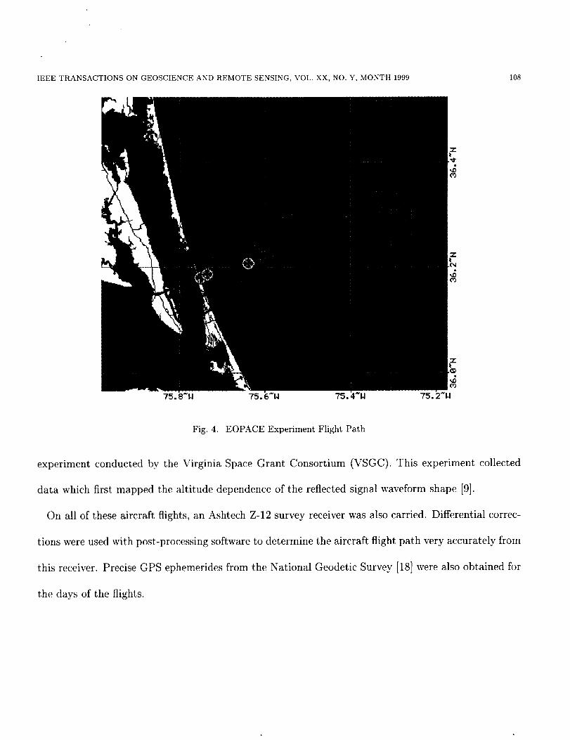
The flight path of the TOPEX underflight is shown in figure 3, and that of the EOPACE experiments
is shown in figure 4. Figure 4 also shows the location of 3 data buoys.
On August 22, 1998, the SDMR hardware was carried to altitudes in excess of 25 km on a balloon
IEEE TRANSACTIONS ON GEOSCIENCE AND REMOTE SENSING, VOL. XX, NO. Y, MONTH 1999 108
Fig. 4. EOPACE Experiment Flight Path
experiment conducted by the Virginia Space Grant Consortium (VSGC). This experiment collected
data which first mapped the altitude dependence of the reflected signal waveform shape [9].
On all of these aircraft flights, an Ashtech Z-12 survey receiver was also carried. Differential correc-
tions were used with post-processing software to determine the aircraft flight path very accurately from
this receiver. Precise GPS ephemerides from the National Geodetic Survey [18] were also obtained for
the days of the flights.

IEEE TRANSACTIONS ON GEOSCIENCE AND REMOTE SENSING, VOL. XX, NO. Y, MONTH 1999
P
109
III. POST PROCESSING
OST processing was performed on the raw, or level 0 data from the receiver which accomplishes
two basic functions: determining the location of the specular reflection point on the surface
of the ellipsoidal Earth, and re-alignment of each (1/2 code chip spaced) correlator sample in code
delay relative to the specular point. This was done to more precisely reference the measurement to the
location of ground truth (the location of the specular point can be several kilometers from the aircraft
ground track) and to continuously map the waveform samples at finer than 1/2 chip precision.
This realignment was performed through use of the navigation data from the aircraft and the NGS
ephermides. Timing of the measurements was either provided from the GPS solution (in the case of
4 or more direct satellites tracked), or from a single satellite in the case of the PDMR. The true path
length difference of a specular reflection from the surface of the WGS-84 ellipsoid was computed by
minimizing the total path length of a reflected signal.
PL
(xL- Xs(¢s,:_s))2+
(YL- gs(¢s, :_s))2+
(z_- zs(,s, As))2
(Xcps - Xs(_s, _s))2+
+ (YAPS- Ys(Os, As))2+ (3)
\ (zcps- zs(O_,A_)) _
The Earth-centered Earth-fixed coordinates of the LHCP antenna phase center (XL, YL, ZL) were
obtained from the differentially corrected Ashtech flight path (assuming level flight). The GPS satellite

IEEE TRANSACTIONS ON GEOSCIENCE AND REMOTE SENSING, VOL. XX, NO. Y, MONTH 1999 110
coordinates (Xaps, YaPs, ZGps) were obtained from the NGS ephemeris. The coordinates of the
specular point (Xs, Ys, Zs) were found by numerically minimizing PL through varying the geodetic
latitude and longitude, Cs and As of a specular point which was assumed to be fixed to lie on the
WGS-84 ellipsoid. The details of these coordinate systems can be found in [11].
The difference between this geometric location of the specular point and the stored code phase
information from sampling the code epoch for each correlator was used to compute the relative delay
between each power sample and the specular point.
This alignment is illustrated in figure 5 (a) and (b).
The correlation power was then normalized to have a constant total area of one half code chip
by dividing by the total integrated power in all range bins at each waveform sample. This removes
changes in the intensity of the incident radiation and was also found to produce results with the lowest
variance. This effectively eliminates the need to calibrate the lower channel correlation values with a
physically meaningful measurement of reflected power and eliminates many uncalibrated effects such
as aircraft attitude motion and the antenna gain pattern.
The result of post-processing is a standard set of "level 1" data. This consists of waveform mea-
surements of the incoherent power, Yk2(Si) at specific code delays, 5k,i. For each k TH waveform sample
(taken at a 1Hz rate for the SDMR and a 10 Hz rate for the PDMR) auxiliary information giving the
specular point location (¢&, Ask) and the GMT of the measurement are also tabulated.
These waveform samples were then used with several retrieval techniques to estimate surface wind
speed. In this paper, summaries are provided for two of these techniques.

IEEE TRANSACTIONS ON GEOSCIENCE AND REMOTE SENSING, VOL. XX, NO. Y, MONTH 1999 111
_4
z3
22o+
0.6
0.5
106 (a.) Level 0 Receiver Data
0.4
0.3O..
0.2o
z 0.1
0
-0.1-2
Illl,I ,
2 4 6 8 10
Delay Bin Number
(b.) Normalized and Georeferenced Data
0
Code Delay (Chips)
0.6(d.) Least Squares Fit to Data
0.5
0.4
0.3O..
E_ 0.2
o0.1
-0.1-2 0 2 4
Code Delay (Chips)
(e.) Post-Fit Residuals
°11 :
,I' ,tloo°....'....,tli,,"I _oo_. i,jj, o,/ '"
2 4 -2 0 4
Code Delay (Chips)
(c.) Corrected Level 1 Data0.6
0.5
0.4 i
' i_. o.a
Z
ol |ll=lal
-0.i 8
-2 0 2 4
Code Delay (Chips)
July 15, 1999 TOPEX Underflight
Altitude: 8km
Satellite Elevation: 73 deg.
80 sec of 10Hz PDMR data (800 samples)
Retrieval: 3.2 trds
TOPEXMeasurement: 2-3.5 m/s
Fig. 5. Example Data Post Processing

IEEE TRANSACTIONS ON GEOSCIENCE AND REMOTE SENSING, VOL. XX, NO. Y, MONTH 1999 112
IV. ESTIMATION TECHNIQUES
A. Wind Speed Estimation Using the Wave form Trailin9 Edge
This retrieval technique includes the generation of sets of modeled waveforms, the normalized power
versus time delay with respect to the nominal specular point, for various wind speeds. The theoretical
model by Zavorotny and Voronovich [6] was used to generate waveforms. The model used the elevation
spectrum of wind-driven sea surface derived by Elfohaily et al. [12] taking into account fetch-limited
conditions. For this research, we assumed that seas are well-developed with an unlimited fetch. The
trailing edge of the waveform taken in a logarithmic scale was used for the estimation as the most
sensitive part to surface wind speeds.
The measured signals were normalized by the integral power observed in delay bins within the
expected range of the glistening zone. Measurements showed that there is no strong signal correlation
between the top and bottom channels. The total reflected power is not expected to depend on surface
statistics and can be used as a normalization factor.
A comparison was made between data collected at 3.8 km altitude on the EOPACE experiment and
the theoretical model developed by Zavorotny and Voronovich. To smooth this data, a 150 second
sliding average was applied to the raw reflected GPS measurements. As described above, an adaptive
signal normalization, which generates a constant area waveform was used to cancel out the uncalibrated
effects of antenna gain, aircraft attitude motion, and difference in cable loss and front-end gain between
the direct and reflected signals. This data was "binned" across discrete code delays measuring one
half-code chip. 'This corresponds to 150 meters in range resolution). To account for variations in

IEEETRANSACTIONSONGEOSCIENCEANDREMOTESENSING,VOL.XX,NO.Y,MONTH1999 113
the noisefloor of the reflectedsignal, the correlation powerrecordedin the last four delay bins and
subtractedit from the reflectedsignal. The trailing edgeslopeona decibelscalewasestimated with a
leastsquaresfit of a straight line to the measuredwaveformsbetween5 and 20dB. This wascompared
to the theoreticalmodel predictionsusingvariousincrementalwind speeds.The estimatedwind speed
wasobtained by interpolating the measuredslopesbetweenthe modeledones.
The TOPEX-altimeter over-flight covereda wide range of wind speedsranging from 0.5 m/s to
8.7 m/s within a ground distanceof about 40 kin. After processingthe data, the TOPEX-indicated
geographicarea wasmatched with the location of GPS measurements.Two different waveformsfor
PRN15wereobtained for 0.5 and 8.7 m/s wind speedsasindicated in Figure 6. This figure displays
the modeledvaluesfor these two different wind speeds. As predicted by the model, a higher wind
speedresultsin a wider waveformwith a loweredpeak power. Note that agreementbetweenmeasured
and modeledwaveformscan be assessedon the trailing edgeof the waveformbetween5 and 20 dB
asdescribedearlier. The measuredand modeledwind speedsshowedgood agreementfor PRN15 in
Figure 7.
It canbeconcludedthat for the lower0.5m/s wind speed,the agreementappearednot to beasgood
asfor the 8.7 m/s wind speed. This could bedue to the fact that at lower wind speedthe Rayleigh
criteria of diffusescattering may be violated, possibly limiting the accuracyof modeledwaveform at
lower than 2 to 3 m/s wind speeds. In Figure 7, we displayed the processed waveform for PRN19
along with the predicted waveforms for 6, 8, 10, and 12 m/s. TOPEX wind measurement indicated
an 8.7 m/s. The figure clearly shows that the observed wind speed is between 8 and 10 m/s. We have
found the trailing edge of the waveform to be very stable between 5 and 20 dB , therefore we used

IEEE TRANSACTIONS ON GEOSCIENCE AND REMOTE SENSING, VOL. XX, NO. Y, MONTH 1999 114
O
O
Z
0
-5
-10
-15
-20
-25
-30
0 2 4 6 8 [0 12 14 16
Delay in Half-Chips
Fig. 6. Predicted and measured waveforms for low and high wind speeds for PRN15
._=
O
N
O
Z
-5
-I0
-15
-20
-25
-30
2 4 6 8 10
Average Measured Waveform
Delay in Half-Chips
.10 m/s
18m/s
12 14 16
Modeled W aveforms
Fig. 7. Predicted and measured waveforms for 8.7 m/s wind speed (PRN19)

IEEETRANSACTIONSONGEOSCIENCEANDREMOTESENSING,VOL.XX,NO.Y,MONTH1999
12
10
8
e.,
"_ 6
2
TOPEX-Measured Wind Data
• Wind Speed Estimates Using PRN15 T -r -,-
• Wind Speed Estimates Using PRN19
i,____.t2e,.I i I I I I I I I
36.7 36.6 36.5 36.4 36.3 36.2 36.1 36 35.9 35.8
Latitude in Degrees
115
Fig. 8. Estimated wind speed using PRN15 and PRN19 and TOPEX ground truth
that region to routinely infer surface wind speeds.
For every TOPEX wind speed measurement, the trailing edge slope was estimated using the measured
waveforms between 5 and 20 dB and the theoretical model using various incremental wind speeds. The
estimated wind speed was obtained by interpolating the measured slopes between the modeled ones.
In Figure 8, we displayed both the TOPEX measured wind speeds and our estimated ones using GPS
data from two different satellites: PRN15 and PRN19. The 1 -a error bars were also displayed for the
measured wind speeds. The figure shows that the error bars are larger for higher wind speed. This is
due to the fact that for higher wind speeds the separation between two waveform slopes, corresponding
to two separate wind speeds, are smaller than the separation between two wind speeds at smaller wind
speeds. Furthermore, the figure indicates that wind speeds estimated independently using the two
satellites show good agreement with the TOPEX-measured wind data.

IEEE TRANSACTIONS ON GEOSCIENCE AND REMOTE SENSING, VOL. XX, NO. Y, MONTH 1999
0
-5
"_ -10
-15
Z-20
-25
6 8 10 12 14 16 18 20 22
+ Average Measured Waveform _ Modeled Waveforrm
Delay in Half-Chips
24
116
Fig. 9. Predicted and Measured Waveforms for PRN04 at 6.5 km altitude.
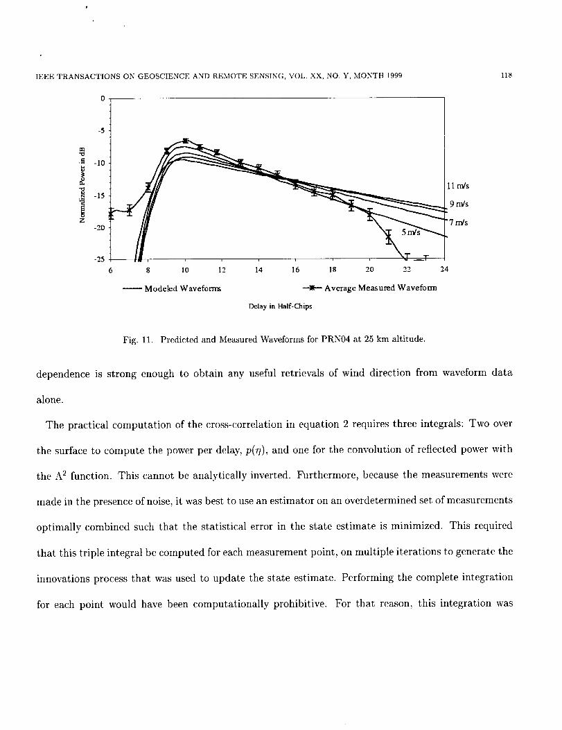
We have also processed the surface-reflected GPS data from the VSGC Balloon Experiment. Here,
waveforms are presented for three different altitudes for the same PRN04 satellite. In Figure 9, a
waveform for PRN04 collected at an altitude of 6.5 km is shown. The modeled theoretical waveforms
for wind speeds 5, 7, 9, 11 m/s are also plotted. Figure 10 presents a waveform for the altitude 12 km,
whereas Figure 11 displays the highest altitude of 25 km. The comparison of these figures reveal that
the waveform trailing edge slope and peak power decreases with height as predicted by the theoretical
model. A comparison between modeled and measured waveforms suggests that the wind speed might
have been between 5 to 7 m/s around that region. The nearby buoy data indicates a 5 m/s wind
speed for the vicinity of the experiment. Even at 25 km altitude a strong reflected signal was observed
showing a straight line trailing edge (on a logarithmic scale) allowing the estimation of surface wind

IEEE TRANSACTIONS ON GEOSCIENCE AND REMOTE SENSING, VOL. XX, NO. Y, MONTH 1999 117
0
-5
"_ -10
-25
11 rr/s
m/s
7 m/s
5 m/s
6 8 10 12 14 16 18 20
+ Average Measured Waveform _ Modeled Waveforms
Delay in Half-Chips
Fig. 10. Predicted and Measured Waveforms for PRN04 at 12 km altitude.
speed. These results show that similar estimates of 5 m/s wind speed were obtained at three different
altitudes up to 25 km.
B. Series Approximation of Waveform Shape
Conceptually, existing analytical models [6] and [4] generate waveforms, Y2(5), with a function
relationship to wind speed.
y2(5) = f(5, V_) (4)
Only the magnitude of wind speed (V_) was considered in this study. The use of the anisotropic
surface statistics [6] (or a skewed non-Gaussian probability density function) [4] would show that the
waveform shape is weakly dependent upon wind direction as well. It has not been determined if this
IEEE TRANSACTIONS ON GEOSCIENCE AND REMOTE SENSING, VOL. XX, NO. Y, MONTH 1999
0
118
-5
"i°_ -15-10 119m/m/i
-25 .....
6 8 10 12 14 16 18 20 22 24
Modeled Waveforrm _ Average Measured Waveform
Delay in Half-Chips
Fig. 11. Predicted and Measured Waveforms for PRN04 at 25 km altitude.
dependence is strong enough to obtain any useful retrievals of wind direction from waveform data
alone.
The practical computation of the cross-correlation in equation 2 requires three integrals: Two over
the surface to compute the power per delay, p(zl), and one for the convolution of reflected power with
the A 2 function. This cannot be analytically inverted. Furthermore, because the measurements were
made in the presence of noise, it was best to use an estimator on an overdetermined set of measurements
optimally combined such that the statistical error in the state estimate is minimized. This required
that this triple integral be computed for each measurement point, on multiple iterations to generate the
innovations process that was used to update the state estimate. Performing the complete integration
for each point would have been computationally prohibitive. For that reason, this integration was
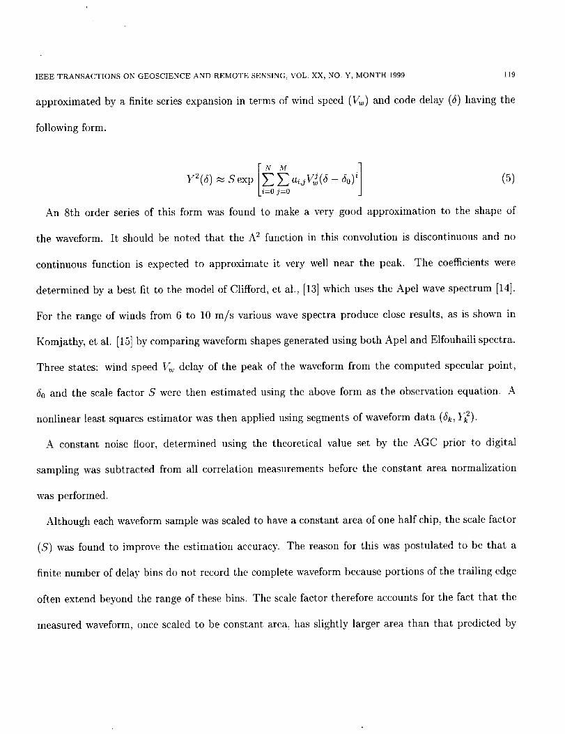
IEEE TRANSACTIONS ON GEOSCIENCE AND REMOTE SENSING, VOL. XX, NO. Y, MONTH 1999 119
approximated by a finite series expansion in terms of wind speed (Vw) and code delay (_f) having the
following form.
]Y_(5) S exp ai,jV_((_ _o) i (5)
ki=0 j=0
An 8th order series of this form was found to make a very good approximation to the shape of
the waveform. It should be noted that the A2 function in this convolution is discontinuous and no
continuous function is expected to approximate it very well near the peak. The coefficients were
determined by a best fit to the model of Clifford, et al., [13] which uses the Apel wave spectrum [14].
For the range of winds from 6 to 10 m/s various wave spectra produce close results, as is shown in
Komjathy, et al. [15] by comparing waveform shapes generated using both Apel and Elfouhaili spectra.
Three states: wind speed Vw delay of the peak of the waveform from the computed specular point,
(_0 and the scale factor S were then estimated using the above form as the observation equation. A
nonlinear least squares estimator was then applied using segments of waveform data ((_k, Y_).
A constant noise floor, determined using the theoretical value set by the AGC prior to digital
sampling was subtracted from all correlation measurements before the constant area normalization
was performed.
Although each waveform sample was scaled to have a constant area of one half chip, the scale factor
(S) was found to improve the estimation accuracy. The reason for this was postulated to be that a
finite number of delay bins do not record the complete waveform because portions of the trailing edge
often extend beyond the range of these bins. The scale factor therefore accounts for the fact that the
measured waveform, once scaled to be constant area, has slightly larger area than that predicted by

IEEE TRANSACTIONS ON GEOSCIENCE AND REMOTE SENSING, VOL. XX, NO. Y, MONTH 1999 120
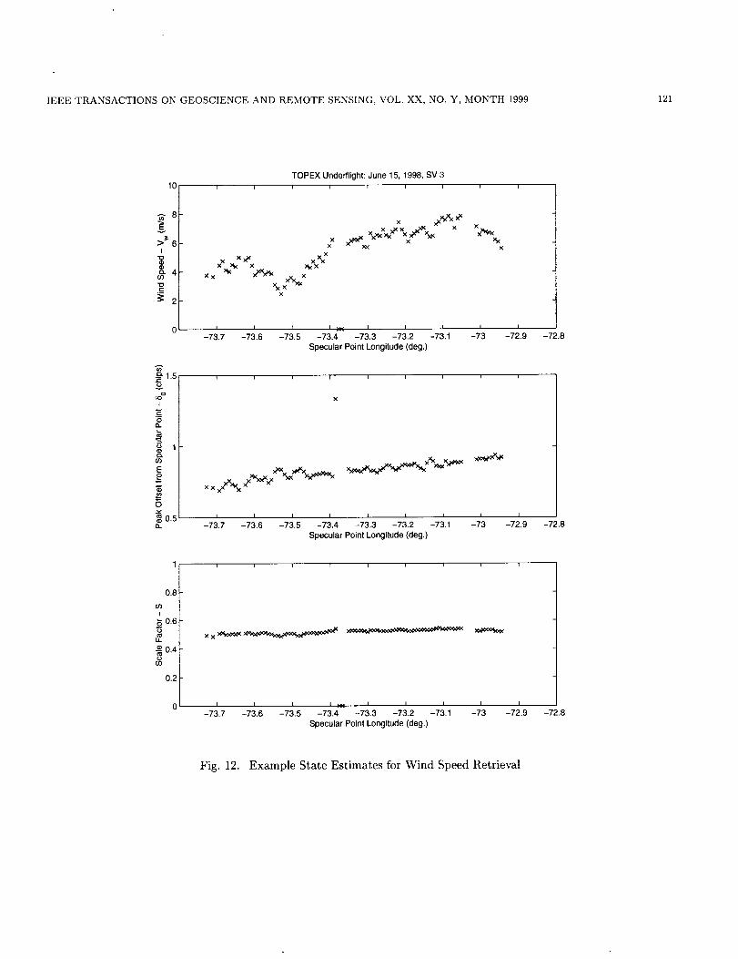
theory. Using the state 5o effectively calibrated the relative delay between the direct and the reflected
signal path lengths. The variance in this state could also being interpreted as an upper bound on
the practical accuracy achievable using the reflected GPS signal as an altimeter. The state estimate
in figure 12 suggests that this uncertainty is approximately 0.1 chip, or 30 meters. Figure 12 shows
the time history of these three states for a typical segment of reflected GPS data collected under the
TOPEX ground track.
Three effects and receiver anomalies were not accounted in these signal models. These were identified
and corrected before the data was processed by the least squares estimator. Editing the data in this
manner was found to improve the performance of this estimator and removed most of the outlying wind
speed estimates. However, as the single outlier point in the estimate for 5o near -73.4 deg. in figure 12
shows, there were occasionally these anomalies which were not detected. With an improved residual
monitoring process these cases may be eliminated in the future. First, the total power in all delay
bins was computed and if this fell below a threshold, then the complete waveform was rejected. This
eliminated measurements made over land, and time in which the receiver had not acquired a strong
reflected signal. Second, occasionally slips by an integer number of half code chips in the spacing of the
delay bins was observed (as demonstrated by the two superimposed waveforms on figure 5 (b)). This
anomaly was identified and corrected by adding or subtracting an integral number of half-code chips
to the array of delay variables (5) on each waveform until the maximum recorded cross correlation
measurement was within 1 code chip of the specular reflection point. This correction is illustrated in
figure 5 (c). The outlier shown near -73.4 deg. was the result of failure to detect one of these slips.
An improved receiver design (to eliminate this failure at the source) combined with a better residual
IEEE TRANSACTIONS ON GEOSCIENCE AND REMOTE SENSING, VOL. XX, NO. Y, MONTH 1999 121
TOPEX Underflight: June 15, 1998, SV 310 , , _ , J
8
>_= 6I
"oo
o. 4
_ 2
_" 1.5,
I
E
o.ffl
E
O
_0.5D.
0.8
8 0.6
0.4
0.2
x_x_xxx
Xx_ XxxKx_ :_x
x
I I 1 I )$( I I I | I
-73.7 -73.6 -73.5 -73.4 -73.3 -73.2 -73.1 -73 -72.9
Specular Point Longitude (deg.)
i , , 1 J l , i l
X
I i I I I I I
-73.7 -73.6 -73.5 -73.4 -73.3 -73.2 -73.1
Specular Point Longitude (deg.)
_7i3 J-72.9
, , i J i , i , r
I I I I )iK I I I / I
-73.7 -73.6 -73.5 -73.4 -73.3 -73.2 -73.1 - 73 -72.9
Specular Point Longitude (deg.)
-72.8
-72.8
-72.8
Fig. 12. Example State Estimates for Wind Speed Retrieval

IEEETRANSACTIONSONGEOSCIENCEANDREMOTESENSING,VOL.XX,NO.Y,MONTH1999 122
monitoring processcould reducethesecases.
The third effect identified wasanother receiverartifact in which the leadingedgeof the waveform
extendedearlier than the first correlator. In thesecases,there was correlation power in the earliest
correlator powerbin. Attempts to blindly fit the function definedaboveto this situation resulted in a
wider than required waveformshapeand consequentlya higher wind speed.Individual waveformsin
which this correlation power exceedssomethresholdare deletedfrom the ensemble.Although most
of the information about the surfaceslopestatistics is containedin the trailing edgeof the waveform,
this method makesuseof the complete shapeand the presenceof this anomaly resulted in higher
than expectedwind speedestimatesbecauseof the tendency to fit a "wider" function to waveforms
truncatedin this manner. At presentall that wasdoneto correct for this effectis to deletethe waveform
samplefrom the ensemblealtogether. It may be possibleto include zero-valuedpower measurements
at time delaysearlier than the start of the measurementssoas to forcethe curve fitting algorithm to
convergeto zero for delaysearlier than -1 codechip relative to the specularpoint. This correction
would be justified becauseno reflectedpower could be receivedearlier than the specularpoint and
thereforeno correlation could exist earlier than 1 chip prior to the specularpoint. Methods described
earlierwhich useonly the trailing edgedata would not sufferfrom this anomaly.
Finally, a residualmonitoring processisusedin whicha thresholdis seton the sumsquareof residuals
in onewaveform.This wascomputedfrom the differencebetweenthe observedand computed power
following the least squaresestimate for the k Tt_ waveform.
rk = Y_(Y_i- Y_((_k,i, V_, S, 6o)) 2 (6)i

IEEE TRANSACTIONS ON GEOSCIENCE AND REMOTE SENSING, VOL. XX, NO. Y, MONTH 1999 123
in which Y_ is the function from equation (5) computed with the estimated state vector ($_, S, 69). The
k TtI waveform was rejected from the ensemble when rk exceeded a threshold. The complete ensemble
(less the waveforms which were rejected) was then processed through the least squares estimator a
second time. Figure 5 (d) shows the resulting best fit waveform to the data from figure 5 (c). Figure
5 (e) shows the post fit residuals for each measured waveform.
Results from this estimator were compared against the TOPEX wind speed retrievals for the series
of TOPEX underflights and against the surface truth measured from buoys during the EOPACE
experiment. Figure 13 shows a comparison between the results of this method operating on PDMR
data and TOPEX wind speed retrieval. These retrievals were performed on 100 second batches of
waveform measurements using coefficients, ai,j computed for the altitude and average elevation of each
GPS satellite from which data was collected. Longitude of the TOPEX ground track and the specular
point are used as the independent variable. These results indicate at most a 2 m/sec difference between
the two sensors. It should be noted in this comparison that the longitude of the reflection specular
point does not lie on exactly the same line as the TOPEX ground track and that measurements at the
same longitude from the two sensors are not necessarily the physically closest on the ocean surface.
This could explain the apparent shift between the two retrievals on the May 5 data. Also, the largest
discrepancies between the two sensors occur for low wind speeds (4(2 m/s), showing a similar effect to
that observed in the trailing edge slope retrieval.
For the EOPACE experiment, segments of data in which the specular point of the reflection was near
to the three sources of surface truth were used for this comparison. Please refer back to figure 4 for
the location of the ground tracks for these two flights. Measurements with a specular point longitude
IEEE TRANSACTIONS ON GEOSCIENCE AND REIVIOTE SENSING, VOL. XX, NO. Y, MONTH 1999 125
of less than 75.7 deg.W were not used because these were judged to lie too close to the shore line.
Measurements from these points were often significantly lower than that from the recording buoys.
The Met Buoy was 10 km from the shore and was expected to give the best comparison with nearby
measurements. The land area surrounding the shoreline was relatively fiat, however, and therefore the
wind speed measured at all three surface truth locations was found to be similar. Wind direction was
obtained from the Duck meteorological station.
For retrievals of the EOPACE data, batches of 300 seconds of waveform data were processed for
each state estimate. A set of coefficients ai,j were computed for and altitude of 3.8 km and elevation
increments of 15 degrees. The set for the elevation closest to the average elevation for a given satellite
was used in the estimator. This simplification was justified because the shape of the waveform is not
strongly dependent upon grazing angle for the satellite elevations used.
Results from this are shown in figures 14 through 17. The comparison data from the Flux and Met
research buoys was averaged for 5 minutes near the time of each overpass. The standard deviation of
this measurement is also illustrated by the errorbars on these figures. Duck wind speed measurement
was taken as the average of the three measurements recorded nearest recorded time to the overflights.
These plots show in most cases an agreement to better than 2 meters per second between the reflected
GPS retrievals and the surface truth data.
V. CONCLUSIONS AND FUTURE WORK
These experiments have demonstrated reliable retrievals of geophysical data using the power versus
delay waveform recorded from bistatically scattered GPS signals. The two airborne data campaigns

IEEE TRANSACTIONS ON GEOSCIENCE AND REMOTE SENSING, VOL. XX, NO. Y, MONTH 1999 126
. 75.6"W 75 75.4~g
14
_t2
_e
_6
4
i
J/DUCK
O
+x
NetI
-75.75
i i i ,
Flux x sv 27 (pass1) J_ BuoyData
x_ x
x x xx xx
-75.7 -75 65 -75,6 -75 55 -75.5 -75 45 -75,4
14
4 DUCK
_75175
' Flux_ 'm
o0p ,
II xm
Net
, ,. ,-75.7 -75 65 -75.6
oe
m x x_
x X x
x SV 15
_ SV 27 (pass 1)BuoyData
-75'.55 A-75.5 -75'.45 -75.4
Specular Point Longitude (deg)
Fig. 14. EOPACE Data Comparison: March 1, 1999
75. 75. 75. 713. N
15
°ti
DUCK Flux
0 x x _ x
-75,75 -75.7 -75 65
i 1 i
DUCK Met
xi X
-75175 -75.7 _751,65
, i i
L x sv 18 (pass 1)1BuoyData
x x x x x xx
i i I i-75.6 -75.55 -75.5 -75.45 -75.4
Flux x sv 18 (pass 2)
Buoy Data
xx x x x x x
-75.6 -75 55 -75.5 -75 45 -75.4
15 ,
JDucK Met
._c 51- 0 ®/
| = ,-7525 -75.7
i
Flux
x J x x x
x _ x
_751.65 I-75.6 -75'.55
Specular Point Longitude (deg)
i
SV 19
_)-- Buoy Data I
-75.5 -75 45 -75.4
Fig. 15. EOPACE Data Comparison: March 5, 1999

IEEE TRANSACTIONS ON GEOSCIENCE AND REIVIOTE SENSING, VOL. XX, NO. Y, MONTH 1999 127
75 . 7"g 75 . 6"g 75 • 75.4"U 75.3 .I
= i14
_12 O
g,0® } .,_6
_ 6 DUCK4
2 -75 75 -75.7
i i
14
-._- 12 0
v
6 DUCK4
,. ,2 -75 75 -75.7
i i
Flux
. ¢e
x
x mmx
x SV 31 (pass 1)• SV 19 (pass 1)
---O-- Buoy Data
oe
x x
-75.65 -75.6 -75 55 -75.5 -75 45 -75.4
' _ Flux
(_ m •O
m m
i i
x SV 31 (pass 2)
.__ SV 19 (pass 2)Buoy Data
_75n65 n i-75.6 -75'.55 -75.5 -75'.45 -75.4
Specular Point Longitude (deg)
Fig. 16. EOPACE Data Comparison: March 8, 1999
75,7~g 75 75. 75° 4"14 75, 3
15 /
;_ 5 DUCt x x
xx x
x SV31 (pass 1)_ Buoy Data
i-75155 -75.5 -75145 -75.4
x
x x x x x
x SV 31 (pass 2)_ Buoy Data
, ,.-75.5 -75 45 -75.4
Fluxt L i
-75.75 -75.7 -75.65 -75,6
15 _
_" t _ FluxI0 0 x x x x
°f t_=5 DUCK ....-75,75 -75,7 -75,65 -75,6 -75.55
15j
_,Ol- o _Flu'xx
i f
x SV 13 IBuoy Data 1
x x x
i
-75.5-75.75
a
-75.7
x xx
x
i i I
-75.65 -75.6 -75,55 -75145 -75,4
Specular Point Longitude (deg)
Fig. 17. EOPACE Data Comparison: March 12, 1999

IEEE TRANSACTIONS ON GEOSCIENCE AND REMOTE SENSING, VOL. XX, NO. Y, MONTH 1999 128
evaluated in this study provide reference data to compare retrieval techniques. Future experimentation,
however, should be conducted under better known conditions and with better ground truth. Retrieval
methods could be improved through better electromagnetic models of the reflection process, specifically
effects of polarization. Also, statistical parameters describing the random rough surface could be used
as the estimation state as opposed to a geophysical parameter such as wind speed. This separates
the more fundamental geometric optics measurement model from the empirical relationship between
geophysical data (wind vectors) and surface statistics (mean square slope and wave spectra). Another
area of improvement is the incorporation of multiple satellites into the same estimator, for measurement
situations in which the specular point locations are close enough together such that they can be assumed
to be samples of the same surface process. An understanding of the statistics of the waveform power
samples, from both experimental and theoretical sources, would improve the estimator design and
provide a rational basis for selecting data weights and thresholds on the residual monitoring.
Directional information may also be retrieved from the reflected signal through the mapping of the
waveform in both code delay and Doppler frequency. This would require enhancements in the receiver
architecture and is the next step in the development of this hardware.
REFERENCES
[1] Katzberg, S. J., Garrison, J. L., Coffey, N. C., and Kowitz, H. R., Method and System for Monitoring Sea State Using
GPS, application filed with the U.S. Patent and Trademark Office, 8 January 1998.
[2] Kaplan, Elliot D., ed., Understanding GPS Principles and Applications,Artech House Publishers, Boston, 1996.
[3] Parkinson, Bradford W., Spilker, James J., Axelrad, Penina, and Enge Per, eds. Global Positioning System: Theory and
Applications Volume I, AIAA, Washington DC, 1996.
[4] Lin, B., Katzberg, S. J., Garrison, J. L., and Wielicki, B., The Relationship Between the GPS Signals Reflected from Sea

IEEETRANSACTIONSONGEOSCIENCEANDREMOTESENSING,VOL,XX,NO,Y,MONTH1999 129
SurfacesandtheSurfaceWinds:ModelingResultsandComparisonsWithAircraftMeasurements,Journal of Geophysical
Research - Oceans,in press.
[5] Cox, C. and Munk, W., Measurement of the Roughness of the Sea Surface from Photographs of the Sun's Glitter, Journal of
the Optical Society of America, 17ol. 44, No. 11, pp. 838-850, November 1954.
[6] Zavorotny, V. U., and Voronovich, A.G., Scattering of GPS signals from the ocean with wind remote sensing application,
IEEE Trans. Geosci. Remote Sensing,in press.
[7] GEC Plessey Semiconductors, Global Positioning Products Handbook, August 1996.
[8] Garrison, J. L., Katzberg, S. J. and Hill, M. I., Effect of Sea Roughness on Bistatically Scattered Range Coded Signals from
the Global Positioning System, Geophysical Research Letters, Vol. 25, No. 13, pp. 2257-2260, July I, 1998.
[9] Garrison, James L., and Katzberg, Stephen J., "The Application of Reflected GPS Signals to Ocean Remote Sensing," Remote
Sensing of Environment, in press.
[10] National Oceanic and Atmospheric Administration (NOAA), NDBC Data Availability Summary, NDBC Technical Document
96-03, Stennis Space Center, MS, February 1997.
[11] Hofmann-Wellenhof, B., Lichtenegger, H., and Collins, J., GPS Theory and Practice,Springer-Verlag, New York, 1992.
[12] Elfouhaily, T., B. Chapron, K. Katsaros, and D. Vandermark, "A Unified Directional Spectrum for Long and Short Wind-
Driven Waves," J. Geophys. Res., 102,15,781-15,796.
[13] Clifford, S.F., V.I.Tatarskii, A. G. Voronovich and V.U.Zavorotny, "GPS Sounding of Ocean Surface "Waves: Theoretical
Assesment,in Proceedings o] the IEEE International Geoseience and Remote Sensing Symposium: Sensing and Managing the
Environment,pp. 2005-2007, IEEE, Piscataway, N. J., 1998.
[14] Apel, John R., "An Improved Model of the Ocean Surface Wave Vector Spectrum and its Effects on Radar Backscatter,"
Journal of Geophysical Research, Vol. 99, No. C8, August 15, 1994, pp. 16,269-16,291.
[15] Komjathy, A., Zavorotny, V., Axelrad, P., Born, G. H., and Garrison, J. L., GPS Signal Scattering from Sea Surface: Wind
Speed Retrieval Using Experimental Data and Theoretical Model, Remote Sensing of Environment, in press.
[16] Garrison, J. L., Katzberg, S. J., and Howell, C. T., Detection of Ocean Reflected GPS Signals: Theory and Experiment,
Proceedings IEEE Southeastcon, Blacksburg, VA, p. 290-294, 12-14 April 1997.
[17] Graf, J., Sasaki, C., Winn, C., Lui, W. T., Tsai, W., Freilich, M., and Long, D., NASA Scatterometer Experiment, ACTA
Astronautica,Vol. 43, No. 7, pp 367-407, 1998.
[18] National Oceanic and Atmospheric Administration (NOAA), NOAA Technical Report NOS 133 NGS 46, Extending the
National Geodetic Survey Standard Orbit Formats, November 1989

IEEETRANSACTIONSONGEOSCIENCEANDREMOTESENSING,VOL.XX,NO.Y,MONTH1999 130
[19]Shaw,JosephA.,Churnside,JamesH.,"Scanning-laserGlintMeasurementsofSea-SurfaceSlopeStatistics,"Applied Optic-
s,Vol. 36, No. 18, June 1997, pp 4202-4213.