reduction of onu buffering for pon/vdsl hybrid access networks
TRANSCRIPT

University of Texas at El PasoDigitalCommons@UTEP
Open Access Theses & Dissertations
2013-01-01
Reduction Of Onu Buffering For Pon/vdsl HybridAccess NetworksElliott Ivan GurrolaUniversity of Texas at El Paso, [email protected]
Follow this and additional works at: https://digitalcommons.utep.edu/open_etdPart of the Electrical and Electronics Commons
This is brought to you for free and open access by DigitalCommons@UTEP. It has been accepted for inclusion in Open Access Theses & Dissertationsby an authorized administrator of DigitalCommons@UTEP. For more information, please contact [email protected].
Recommended CitationGurrola, Elliott Ivan, "Reduction Of Onu Buffering For Pon/vdsl Hybrid Access Networks" (2013). Open Access Theses & Dissertations.1637.https://digitalcommons.utep.edu/open_etd/1637

REDUCTION OF ONU BUFFERING FOR PON/VDSL
HYBRID ACCESS NETWORKS
ELLIOTT IVAN GURROLA
Department of Electrical and Computer Engineering
APPROVED:
Michael P. McGarry, Ph.D., Chair
John A. Moya, Ph.D.
Patricia J. Teller, Ph.D
Benjamin C. Flores, Ph.D.Dean of the Graduate School

Copyright c©
by
Elliott I. Gurrola
2013

A mis padres que nos apoyan con todo su amor y carino.
To my aunt Olga who has always been here for me,
making my journey less harsh and more pleasant.

REDUCTION OF ONU BUFFERING FOR PON/VDSL
HYBRID ACCESS NETWORKS
By
ELLIOTT IVAN GURROLA, B.S.E.E
Presented to the Faculty of the Graduate School of
The University of Texas at El Paso
in Partial Fulfillment
of the Requirements
for the Degree of
MASTER OF SCIENCE
Department of Electrical and Computer Engineering
THE UNIVERSITY OF TEXAS AT EL PASO
December 2013

Acknowledgements
I would first like to thank my advisor Dr. Michael McGarry for his invaluable guidance. Dr.
McGarry has been more than just an academic advisor, he has also served as a mentor and guide
in personal matters, always willing to provide advice and share his experiences with his students.
Dr. McGarry has also provided a research assistantship which allowed me purse my degree for
which I will always be really grateful.
I would also like to extend my gratitude to Dr. John Moya and Dr. Patricia Teller for kindly
agreeing to serve in my thesis committee.
Finally, I would like to thank the Texas Instruments Foundation for its support in funding my
education.
v

Table of Contents
Page
Acknowledgements . . . . . . . . . . . . . . . . . . . . . . . . . . . . . . . . . . . . . . . . v
Table of Contents . . . . . . . . . . . . . . . . . . . . . . . . . . . . . . . . . . . . . . . . . vi
List of Tables . . . . . . . . . . . . . . . . . . . . . . . . . . . . . . . . . . . . . . . . . . . viii
List of Figures . . . . . . . . . . . . . . . . . . . . . . . . . . . . . . . . . . . . . . . . . . ix
List of Symbols . . . . . . . . . . . . . . . . . . . . . . . . . . . . . . . . . . . . . . . . . . xi
1 Introduction . . . . . . . . . . . . . . . . . . . . . . . . . . . . . . . . . . . . . . . . . . 1
1.1 Motivation . . . . . . . . . . . . . . . . . . . . . . . . . . . . . . . . . . . . . . . . 1
1.2 Thesis Structure . . . . . . . . . . . . . . . . . . . . . . . . . . . . . . . . . . . . . 4
2 Hybrid PON/VDSL Access Networks . . . . . . . . . . . . . . . . . . . . . . . . . . . . 6
2.1 Passive Optical Networks . . . . . . . . . . . . . . . . . . . . . . . . . . . . . . . . 7
2.1.1 XG-PON standard . . . . . . . . . . . . . . . . . . . . . . . . . . . . . . . 10
2.2 Digital Subscriber Lines . . . . . . . . . . . . . . . . . . . . . . . . . . . . . . . . 14
2.2.1 VDSL2 standard . . . . . . . . . . . . . . . . . . . . . . . . . . . . . . . . 16
3 Reducing Memory Requirements on Drop-Point Devices . . . . . . . . . . . . . . . . . 19
3.1 Downstream buffering . . . . . . . . . . . . . . . . . . . . . . . . . . . . . . . . . 19
3.1.1 Rate Limiting Device . . . . . . . . . . . . . . . . . . . . . . . . . . . . . . 21
3.2 Upstream buffering . . . . . . . . . . . . . . . . . . . . . . . . . . . . . . . . . . . 22
3.2.1 Ethernet Flow Control . . . . . . . . . . . . . . . . . . . . . . . . . . . . . 22
3.2.2 GATED Flow Control . . . . . . . . . . . . . . . . . . . . . . . . . . . . . 24
4 Performance Analysis . . . . . . . . . . . . . . . . . . . . . . . . . . . . . . . . . . . . . 29
vi

4.1 Downstream Performance . . . . . . . . . . . . . . . . . . . . . . . . . . . . . . . 29
4.2 Upstream Performance . . . . . . . . . . . . . . . . . . . . . . . . . . . . . . . . . 32
4.2.1 Step 1: Control case . . . . . . . . . . . . . . . . . . . . . . . . . . . . . . 33
4.2.2 Step 2: Optimal point for Ethernet flow control . . . . . . . . . . . . . . . 36
4.2.3 Step 3: Performance Comparison between flow control mechanisms . . . . 40
5 Conclusions . . . . . . . . . . . . . . . . . . . . . . . . . . . . . . . . . . . . . . . . . . 48
5.1 Future work . . . . . . . . . . . . . . . . . . . . . . . . . . . . . . . . . . . . . . . 49
Bibliography . . . . . . . . . . . . . . . . . . . . . . . . . . . . . . . . . . . . . . . . . . . 51
Appendix A Simulation Tools . . . . . . . . . . . . . . . . . . . . . . . . . . . . . . . . . 53
A.1 Downstream Simulator . . . . . . . . . . . . . . . . . . . . . . . . . . . . . . . . . 53
A.2 Upstream Simulator . . . . . . . . . . . . . . . . . . . . . . . . . . . . . . . . . . 55
Curriculum Vitae . . . . . . . . . . . . . . . . . . . . . . . . . . . . . . . . . . . . . . . . . 58
vii

List of Tables
2.1 Classification of available DBA algorithms . . . . . . . . . . . . . . . . . . . . . . 10
2.2 Grant Scheduling Frameworks . . . . . . . . . . . . . . . . . . . . . . . . . . . . . 10
2.3 Grant Sizing Policy . . . . . . . . . . . . . . . . . . . . . . . . . . . . . . . . . . . 10
2.4 Grant Scheduling Policy . . . . . . . . . . . . . . . . . . . . . . . . . . . . . . . . 10
4.1 Downstream maximum drop-point buffer length . . . . . . . . . . . . . . . . . . . 30
4.2 Upstream Simulation Plan, step 1 . . . . . . . . . . . . . . . . . . . . . . . . . . . 34
4.3 Maximum Buffer Length with no Flow Control . . . . . . . . . . . . . . . . . . . . 35
4.4 Maximum Loss Rates with no Flow Control . . . . . . . . . . . . . . . . . . . . . 35
4.5 Upstream Simulation Plan, step 2 . . . . . . . . . . . . . . . . . . . . . . . . . . . 36
4.6 Packet Loss observations at 80% traffic load . . . . . . . . . . . . . . . . . . . . . 39
4.7 Upstream Simulation Plan, step 3 . . . . . . . . . . . . . . . . . . . . . . . . . . . 40
A.1 Upstream Simulator Features . . . . . . . . . . . . . . . . . . . . . . . . . . . . . 56
viii

List of Figures
1.1 Structure of a Passive Optical Network (PON). . . . . . . . . . . . . . . . . . . . 1
1.2 Fiber to the drop-point architecture. . . . . . . . . . . . . . . . . . . . . . . . . . 2
1.3 Components of a drop-point device. . . . . . . . . . . . . . . . . . . . . . . . . . . 3
2.1 Physical PON architecture . . . . . . . . . . . . . . . . . . . . . . . . . . . . . . . 7
2.2 PON signal transmission . . . . . . . . . . . . . . . . . . . . . . . . . . . . . . . . 8
2.3 PON REPORT and GRANT messages . . . . . . . . . . . . . . . . . . . . . . . . 9
2.4 XG Transmission Convergence layer . . . . . . . . . . . . . . . . . . . . . . . . . . 11
2.5 XG-TC Service Adaptation Sub-layer . . . . . . . . . . . . . . . . . . . . . . . . . 12
2.6 XG-TC Framing sub-layer . . . . . . . . . . . . . . . . . . . . . . . . . . . . . . . 13
2.7 VDSL point-to-point layout . . . . . . . . . . . . . . . . . . . . . . . . . . . . . . 15
2.8 FDD and TDD comparison . . . . . . . . . . . . . . . . . . . . . . . . . . . . . . 15
2.9 VDSL2 protocol sub-layers . . . . . . . . . . . . . . . . . . . . . . . . . . . . . . . 16
2.10 VDSL2 TPS-TC sub-layer . . . . . . . . . . . . . . . . . . . . . . . . . . . . . . . 17
2.11 VDSL2 PMS-TC sub-layer . . . . . . . . . . . . . . . . . . . . . . . . . . . . . . . 18
3.1 Drop-point Downstream Buffer . . . . . . . . . . . . . . . . . . . . . . . . . . . . 20
3.2 Traffic Shaper placement . . . . . . . . . . . . . . . . . . . . . . . . . . . . . . . . 21
3.3 Effects of Flow Control . . . . . . . . . . . . . . . . . . . . . . . . . . . . . . . . . 24
3.4 Polling time for a drop-point with a single CPE attached . . . . . . . . . . . . . . 25
3.5 Polling time for a drop-point with two CPEs attached . . . . . . . . . . . . . . . . 27
4.1 Placement of Traffic Shapers . . . . . . . . . . . . . . . . . . . . . . . . . . . . . . 30
4.2 Downstream simulation discrepancy . . . . . . . . . . . . . . . . . . . . . . . . . . 31
4.3 Packet Loss Rate at 80% channel load. . . . . . . . . . . . . . . . . . . . . . . . . 38
ix

4.4 PON queueing Delays . . . . . . . . . . . . . . . . . . . . . . . . . . . . . . . . . 42
4.5 Histogram of PON queue delay values for an average presented load of 74% (of
2.488 Gbit/sec). The values are shown for the simulation case of {Online, Limited}
and 3 msec cycle length . . . . . . . . . . . . . . . . . . . . . . . . . . . . . . . . 43
4.6 DSL Queueing Delays . . . . . . . . . . . . . . . . . . . . . . . . . . . . . . . . . . 45
4.7 Maximum per DSL buffer Length . . . . . . . . . . . . . . . . . . . . . . . . . . . 46
4.8 Maximum drop-point aggregate buffer Length . . . . . . . . . . . . . . . . . . . . 47
A.1 Downstream simulator layout . . . . . . . . . . . . . . . . . . . . . . . . . . . . . 53
A.2 Traffic Shaper Pseudo Code . . . . . . . . . . . . . . . . . . . . . . . . . . . . . . 54
A.3 Upstream simulator layout . . . . . . . . . . . . . . . . . . . . . . . . . . . . . . . 56
A.4 Upstream simulator GUI interface . . . . . . . . . . . . . . . . . . . . . . . . . . . 57
x

List of Symbols
CBR Constant Bit Rate
CPE Customer Premise Equipment
DBA Dynamic Bandwidth Allocation
DSL Digital Subscriber Line
DSLAM DSL Access Multiplexer
DTU Data Transfer Unit
FDD Frequency Division Duplexing
FEC Forward Error Correction
FTTdp Fiber to the drop-point
FTTH Fiber to the home
IBLS Input Buffer Limit Scheme
ITU International Telecommunications Union
ONU Optical Network Unit
OLT Optical Line Terminal
PMD Physical Media Dependent
PMS-TC Physical Media Specific Transmission Convergence
PON Passive Optical Network
PTM Packet Transfer Mode
SDU Service Data Unit
TDD Time Division Duplexing
TDM Time Division Multiplexing
TPS-TC Transport Protocol Specific Transmission Convergence
XG-PON 10-Gigabit-Capable Passive Optical Network
XG-TC XG-PON Transmission Convergence Layer
xi

Chapter 1: Introduction
1.1 Motivation
With the increasing proliferation of portable electronics and other smart devices, it is expected
that by 2016 there will be nearly 18.9 billion network connections worldwide compared to the 10.3
billion connections estimated in 2011 [1]. The current trend in the Internet also shows that the
average subscriber bandwidth consumption will increase from 9 Mbit/sec to around 34 Mbit/sec
in 2016 [1], this is in part due to the widespread of high definition video and other emerging
multimedia technologies. In order to keep up with the increasing demand, it would seem logical
that service providers would upgrade their services to offer fiber optical capabilities since this
technology can provide transmission rates on the Gigabit per second range [2]. A common type
of fiber optical network that is commonly used is known as Passive Optical Network (PON). A
basic PON consists on a single Optical Line Terminal (OLT) located at the central office and is
connected to several optical network units (ONU). The structure of a PON is shown in Figure
1.1 and is described in more detail in Chapter 2.
OLT Optical splitter
ONU
ONU
ONU
Fiber connection
Figure 1.1: Structure of a Passive Optical Network (PON).
Deployment of fiber optic cabling and ONU equipment between the OLT and customer
premises, known as fiber to the home (FTTH), represents over 60% of the total cost of set-
ting up a fiber network [3, 4] and in many cases the cost-benefit return is not enough to justify
1

such investment. An alternative solution to reduce costs is to install a single ONU close to the
customer and take advantage of the already deployed copper network to connect the last few
hundred meters needed to reach the customer. This is known as fiber to the drop-point (FTTdp)
[3] or fiber to the curb, shown in Figure 1.2. The left side of the figure shows a PON connected to
a copper Digital Subscriber Line (DSL) network shown on the right. The bridging unit between
these two segments is known as a drop-point device.
OLT Optical splitter
Drop-point devices
Fiber segment
CPE
CPE
CPE Copper segment
CPE
CPE
ONU
DSLAM
ONU
DSLAM
Figure 1.2: A PON (left) is connected to the copper network (right) by using a drop-point deviceas the bridging element.
A drop-point device is a combination of an ONU and a DSL access multiplexer (DSLAM)
that converts the light signals from the PON into electrical signals to be transmitted through the
copper medium. Every drop-point device in the network performs two main tasks. The first task
is to encapsulate the outgoing data packets into the proper format so that they can be converted
into electrical/light signals and vice versa. A detailed explanation of the packet encapsulation
is provided in Chapter 2. The second main function of the drop-point device is to store the
arriving data in its internal memory buffers before transmission, this mainly occurs due to the
large rate mismatch between the two technologies. A drop-point device has one memory buffer
for every attached DSL line as shown in Figure 1.3. From the ONU side, the drop-point device
2
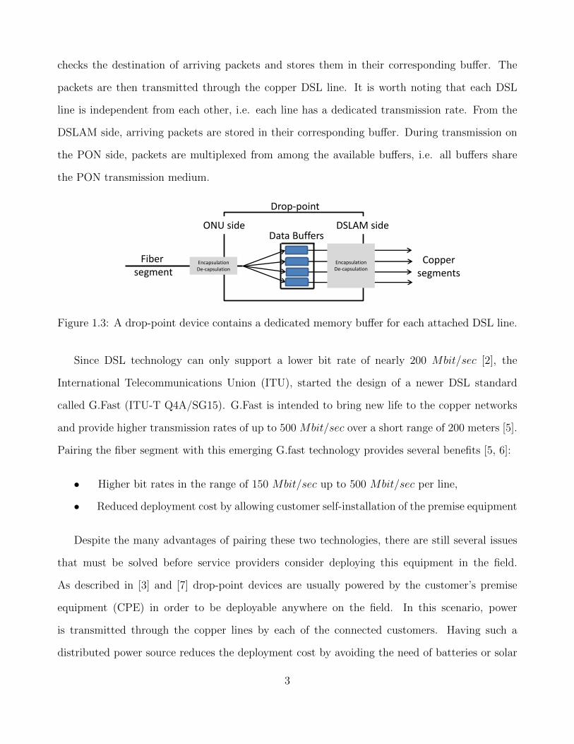
checks the destination of arriving packets and stores them in their corresponding buffer. The
packets are then transmitted through the copper DSL line. It is worth noting that each DSL
line is independent from each other, i.e. each line has a dedicated transmission rate. From the
DSLAM side, arriving packets are stored in their corresponding buffer. During transmission on
the PON side, packets are multiplexed from among the available buffers, i.e. all buffers share
the PON transmission medium.
Drop-point
Data Buffers ONU side DSLAM side
Fiber segment
Copper segments
Encapsulation De-capsulation
Encapsulation De-capsulation
Figure 1.3: A drop-point device contains a dedicated memory buffer for each attached DSL line.
Since DSL technology can only support a lower bit rate of nearly 200 Mbit/sec [2], the
International Telecommunications Union (ITU), started the design of a newer DSL standard
called G.Fast (ITU-T Q4A/SG15). G.Fast is intended to bring new life to the copper networks
and provide higher transmission rates of up to 500 Mbit/sec over a short range of 200 meters [5].
Pairing the fiber segment with this emerging G.fast technology provides several benefits [5, 6]:
• Higher bit rates in the range of 150 Mbit/sec up to 500 Mbit/sec per line,
• Reduced deployment cost by allowing customer self-installation of the premise equipment
Despite the many advantages of pairing these two technologies, there are still several issues
that must be solved before service providers consider deploying this equipment in the field.
As described in [3] and [7] drop-point devices are usually powered by the customer’s premise
equipment (CPE) in order to be deployable anywhere on the field. In this scenario, power
is transmitted through the copper lines by each of the connected customers. Having such a
distributed power source reduces the deployment cost by avoiding the need of batteries or solar
3

panel installation. Even though solar power seems like a promising solution, many locations are
not suitable for solar panels due to the inaccessibility of direct sun light. Because of its reduced
installation and maintenance cost, a copper connection remote powering is usually preferred.
However, when designing such power source for a drop-point device, engineers have to consider
the worst case scenario in which only a single customer is connected to the drop-point device.
Because of this, a single power connection has to be enough to power the system and account for
the power losses due to the relatively long distances between the customer and the drop-point
device. Due to this power limitation, it is not feasible for a drop-point device to perform all the
tasks a regular ONU or a DSLAM would [3].
A possible solution to keep energy consumption at an acceptable level is to delegate some tasks
towards the customer premise equipment (CPE) or the central office’s OLT instead of performing
them at the drop-point device. Another possible way of reducing the energy consumption, and
price, of the drop-point device is by reducing the amount of memory in the device. Having
less memory in the unit means that less transistors have to be placed effectively reducing the
power consumption and the total fabrication cost for each unit. However, reducing the memory
capacity of the drop-point device can have serious consequences on the system performance if
measures are not taken in order to prevent buffer accumulation.
In this study we investigate three methods, described in Chapter 3, that are intended to
reduce the buffer size of the drop-point device. We also provide a performance trade-off analysis
between ONU memory, packet delay and packet loss. Due to the heavy dependence on the
implementation, we do not provide a power consumption analysis of using smaller memories, it
suffice to say that a smaller memory will have a smaller number of transistors with less energy
leakage.
1.2 Thesis Structure
Chapter 2 describes the architecture of a hybrid PON/DSL access network. Section 2.1 first
describes the PON segment of the network including the XG-PON standard used to regulate the
4

fiber link-level communications. Section 2.2 describes the DSL segment of the network including
the VDSL2 and G.Fast standards. Chapter 3 describes our proposed algorithms to reduce the
buffer size in both the downstream (Section 3.1) and upstream (Section 3.2) directions. We pro-
vide a mathematical analysis of the performance of our proposed flow control algorithms. Chapter
4 describes the performance analysis for our proposed flow control algorithms. We describe our
experimental plan and present the obtained simulation results for both the downstream (4.1) and
upstream analysis (4.2). Finally, Chapter 5 presents our conclusion and discusses the avenues
for future work. Appendix A explains the implementation details of the developed simulators.
We also provide a brief overview of the simulator structure.
5

Chapter 2: Hybrid PON/VDSL Access Networks
An access network, also known as the last mile, is the section of a telecommunications network
that connects the end user with its Internet service provider. This section of the network is known
to be the bottleneck in providing high bandwidth services to subscribers. This is because a single
access network usually servers a very limited number of users becoming very cost prohibitive.
In an effort to improve the transmission bit rates in this segment of the network, hybrid access
networks have become the next generation access networks, providing higher bandwidths without
exceeding the cost-benefit necessary for deployment. A hybrid access network is the combination
of at least two technologies working together to provide the function of an access network. There
are many kinds of access networks deployed today whose characteristics vary depending on the
requirements of the subscriber. The most common ones combine a fiber technology on the back-
end, such as PON, and some kind of wireless technology, such as WiFi or WiMAX as the front
end to provide wide user mobility. WOBAN [8] and FiWi [9] are two examples of such hybrid
access networks that have received a lot of attention by the academic community.
In cases where mobility is not required, or whenever traffic security is a priority, such as a
military network, a copper front end technology is more suitable than a wireless technology. In
our study we consider a PON in tandem with the copper VDSL network which is a fast version
of the standard Digital Subscriber Line (DSL). We consider the XG-PON protocol for the PON
segment because of its great popularity in the North America marketplace [10]. In Figure 1.2 we
showed the typical architecture of a PON/VDSL network in which the PON is used as the back-
end connecting the central office of the service provider, the drop-point device and the VDSL
segment that connects the drop-point device to the subscriber’s equipment. An advantage of this
kind of hybrid network is that, in most cases, the copper segment has already been deployed at
the customer’s location.
In this chapter we analyze the behavior of each segment of the access network and provide
details regarding the standard communication protocols used in each segment.
6
2.1 Passive Optical Networks
Central Office
OLT
Optical Splitter
ONU 1
Fiber channel
ONU N
1:N
ONU 2
. . .
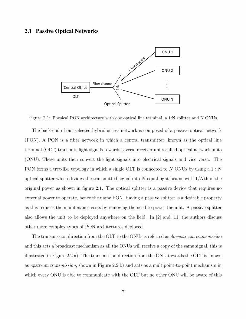
Figure 2.1: Physical PON architecture with one optical line terminal, a 1:N splitter and N ONUs.
The back-end of our selected hybrid access network is composed of a passive optical network
(PON). A PON is a fiber network in which a central transmitter, known as the optical line
terminal (OLT) transmits light signals towards several receiver units called optical network units
(ONU). These units then convert the light signals into electrical signals and vice versa. The
PON forms a tree-like topology in which a single OLT is connected to N ONUs by using a 1 : N
optical splitter which divides the transmitted signal into N equal light beams with 1/Nth of the
original power as shown in figure 2.1. The optical splitter is a passive device that requires no
external power to operate, hence the name PON. Having a passive splitter is a desirable property
as this reduces the maintenance costs by removing the need to power the unit. A passive splitter
also allows the unit to be deployed anywhere on the field. In [2] and [11] the authors discuss
other more complex types of PON architectures deployed.
The transmission direction from the OLT to the ONUs is referred as downstream transmission
and this acts a broadcast mechanism as all the ONUs will receive a copy of the same signal, this is
illustrated in Figure 2.2 a). The transmission direction from the ONU towards the OLT is known
as upstream transmission, shown in Figure 2.2 b) and acts as a multipoint-to-point mechanism in
which every ONU is able to communicate with the OLT but no other ONU will be aware of this
7
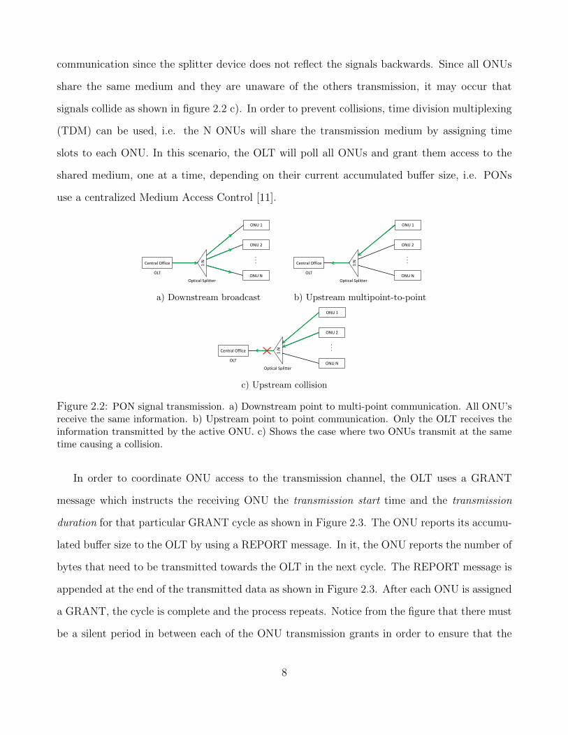
communication since the splitter device does not reflect the signals backwards. Since all ONUs
share the same medium and they are unaware of the others transmission, it may occur that
signals collide as shown in figure 2.2 c). In order to prevent collisions, time division multiplexing
(TDM) can be used, i.e. the N ONUs will share the transmission medium by assigning time
slots to each ONU. In this scenario, the OLT will poll all ONUs and grant them access to the
shared medium, one at a time, depending on their current accumulated buffer size, i.e. PONs
use a centralized Medium Access Control [11].
Central Office
OLT
Optical Splitter
ONU 1
ONU N
ONU 2
. . .
1:N
Central Office
OLT
Optical Splitter
ONU 1
ONU N
ONU 2
. . .
1:N
a) Downstream broadcast b) Upstream multipoint-to-point
Central Office
OLT
Optical Splitter
ONU 1
ONU N
ONU 2
. . .
1:N
c) Upstream collision
Figure 2.2: PON signal transmission. a) Downstream point to multi-point communication. All ONU’sreceive the same information. b) Upstream point to point communication. Only the OLT receives theinformation transmitted by the active ONU. c) Shows the case where two ONUs transmit at the sametime causing a collision.
In order to coordinate ONU access to the transmission channel, the OLT uses a GRANT
message which instructs the receiving ONU the transmission start time and the transmission
duration for that particular GRANT cycle as shown in Figure 2.3. The ONU reports its accumu-
lated buffer size to the OLT by using a REPORT message. In it, the ONU reports the number of
bytes that need to be transmitted towards the OLT in the next cycle. The REPORT message is
appended at the end of the transmitted data as shown in Figure 2.3. After each ONU is assigned
a GRANT, the cycle is complete and the process repeats. Notice from the figure that there must
be a silent period in between each of the ONU transmission grants in order to ensure that the
8

proper light level amplification is configured at the OLT and to prevent any transmission errors
caused by minor timing misalignments. This silent period is known as guard time.
OLT
ONU 1
downstream(TX)
downstream(RX)
upstream(TX)
upstream(RX)
ONU 2 downstream(RX)
upstream(TX)
GRANT 2400
GRANT 5200
2400 + 64 (RPT)
5200 + 64 (RPT)
Guard Time
Figure 2.3: The OLT receives REPORT messages from the ONUs. The OLT then GRANTs each ONUaccess to the transmission medium for certain amount of time. After transmitting the buffered data,the ONU REPORTs its current buffer size to be considered in the next granting cycle.
Because of the bursting nature of the traffic transmitted by the ONUs, it would not be
practical to allocate a fixed amount of the transmission channel to each ONU. In order to provide
a more efficient utilization of the channel, the OLT has to provide statistical multiplexing by using
a dynamic bandwidth allocation algorithm (DBA). The DBA used will let the OLT decide the
order and GRANT duration for each ONU transmission. Choosing the correct DBA algorithm is
important as the system will have a different performance depending on what factors are taken
into consideration to decide the transmission order and duration. For a more detailed analysis of
DBA algorithms and their performance the reader is referred to [12]. According to [12] there are
three criteria by which we can classify the available DBA algorithms, these are shown in Table
2.1.
The Grant Scheduling Framework refers to the moment in time when the OLT should
make the bandwidth assignment, Table 2.2 describes the possible Scheduling frameworks avail-
able. The Grant Sizing Policy refers to the maximum grant size that each ONU will receive,
possible grant sizing policies are shown in Table 2.3. And finally, the Grant Scheduling Policy
9

Table 2.1: Classification of available DBA algorithmsGrant Scheduling Framework Grant Sizing Policy Grant Scheduling Policy
Online Fixed Shortest Processing TimeOflline Gated Shortest Propagation Delay
LimitedLimited with
Excess Distribution
refers to the criteria of how to order the ONU transmissions, i.e. which ONU should transmit
first, Table 2.4 describes the different ordering criteria. In our studies we only consider {Online,
Limited, -} and {Online, Excess, -} DBA algorithms. Since these two DBA algorithms operate
on an Online Framework, no ordering criteria is used as just one ONU is scheduled at a time.
Table 2.2: Grant Scheduling FrameworksGrant Scheduling Framework
Online Bandwidth assignment starts when a single REPORT message isreceived. Only the transmitting ONU is scheduled.
Oflline Bandwidth assignment starts after receiving REPORT from allONUs. All ONUs are scheduled.
Table 2.3: Grant Sizing PolicyGrant Sizing Policy
Fixed Every ONU is granted a fixed grant size of L bytes.Gated Every ONU is granted the previously reported buffer size.Limited Every ONU is granted the reported buffer size up to a maximum value.Limited Excess Similar to Limited, but the unused credits are redistributed among the ONUs re-
questing transmission sizes above the limit. The reader is referred to [12] for a moredetailed explanation of this method.
Table 2.4: Grant Scheduling PolicyGrant Scheduling Policy
Shortest Processing Time ONUs are ordered in ascending order depending on their assignedgrant size.
Shortest Propagation Delay ONUs are ordered in ascending order depending on the one phys-ically closest to the OLT.
2.1.1 XG-PON standard
Because of its popularity in the North America region, in this study we have decided to implement
a 10-Gigabit-capable passive optical network (XG-PON), however, the proposed mechanisms for
10

ONU simplification explained in chapter 3 can be extended to other types of PON/xVDSL hybrid
networks. A XG-PON is a PON system that offers transmission rates of at least 10 Gbit/sec in
either direction and implements the protocols described in the ITU-T G.984.x recommendation
[13] series. These documents describe the behavior and responsibilities of both the transmission
convergence (XG-TC) and the physical media dependent layers. The XG-TC layer combines
the information coming from the various traffic sources and converts it into a single bitstream
suitable for modulation into optical signals. The upper-layer traffic sources transmit their data
in the form of service data units (SDU). This layer is divided into three sub-layers: the service
adaptation sub-layer, the framing sub-layer and the PHY adaptation sub-layer which are shown in
Figure 2.4. The physical media dependent layer encodes the bitstream from the XG-TC layer into
corresponding light waveforms to be transmitted. Because of the nature of our study, we will only
describe the behavior of the XG-TC layer whose details are specified in recommendation ITU-T
G.987.3. Due to the amount of detail contained in these recommendations, only an overview of
these protocols will be provided, the reader is referred to [13] for the complete implementation
details.
Data client
XGTC layer
Upper layer PON control /
management
Service adaptation sub-layer
Framing sub-layer
PHY adaptation sub-layer
XGTC frame / burst
Data client
SDU
XGEM frame
PHY frame / burst
SDU
PMD layer
Figure 2.4: Overview of the XG-transmission convergence layer.
11

I) Service adaptation sub-layer
In the transmitting direction, the service adaptation sub-layer multiplexes, delineates and
encapsulates the arriving upper-layer service data units (SDU). To do so, the arriving SDUs are
encapsulated into a series of XGEM frames, which have an 8-byte header and a word (4-byte)
delineated payload. The multiplexing services of this sub-layer are provided by taking SDUs from
several upper-layer traffic sources and combining them into a single XGEM stream. If a single
SDU does not fit into a single XGEM frame, the SDU will be partitioned and the remainder will
be encapsulated in the next XGEM frame. Only one SDU can be encapsulated on every XGEM
frame. Because of this, XGEM frames will have a varying size ranging from: 4 to 16384 bytes.
In the receiving direction, the XG-TC layer extracts the encapsulated data from XGEM frames,
reassembles fragmented frames and forwards them to its matching upper-layer client. The Port-
ID field in the XGEM header is used to match the data with its corresponding recipient. The
service adaptation layer is shown in Figure 2.5.
Data client n
Service Adaptation Sub-layer
OMCI client Data client A
SDU SDU
OMCI adapter
XGEM engine
User data adapter
PON Management
frames
…
Data Multiplexor
XGEM frames
Header SDU from A
Header SDU from B
Framing sub-layer Header OMCI control
Figure 2.5: The service adaptation sub-layer multiplexes the incoming SDUs, delineates them andfinally encapsulates them into a XGEM frame(s). The service adaptation sublayer uses the Port-IDfield in the XGEM header to determine the recipient.
II) Framing sub-layer
The framing sub-layer multiplexes the PON control and management information with the ar-
riving XGEM frames to form a XGTC frame. An XGTC frame is made up of a header, which
12

contains the control signals, and a payload, which is made up of several XGEM frames. The
framing sub-layer and a simplified version of the upstream/downstream XGTC frame are shown
in Figure 2.6. The XG-TC layer provides 3 channels to control the operation of the PON, two
of which are implemented in this sub-layer. The first channel is the embedded OAM channel
which provides a low latency path for time urgent communication between the OLT and the
ONUs. This channel provides the following functions: upstream timing, bandwidth allocation,
data encryption and ONU power controls. The embedded OAM channel is specially important
since this is where the GRANT and REPORT messages are contained in the downstream and
upstream direction respectively. The second control channel, the PLOAM control channel is
used to control the Physical and the overall XG-TC layers. Some of its functions include: ONU
activation and registration, encryption key exchange and ONU power management. These two
channels are embedded in the header of an XGTC frame. The third control channel supported
by the XG-TC layer corresponds to the upper-layer control signals. These control signals are
seamlessly encapsulated into regular XGEM frames, which are then transmitted as any other
XGEM frame would be. The destination Port ID for these control signals is the receiver control
Client.
XGTC payload
Framing Sub-layer
OMCI client XGTC frame
Service adaptation sub-layer
Upstream DBA control
Header Fields PLOAM partition XGEM Partition
PHY adaptation sub-layer
PLOAM processor
PON management
XGEM frames
XGEM XGEM XGEM
XGTC frame
XGTC frame
Figure 2.6: The framing sub-layer combines the arriving XGEM frames and appends the XGTC headerfields which contain PON control information such as the REPORT and GRANT messages.
III) PHY adaptation sub-layer
The main function of the PHY adaptaion sub-layer is to provide error correction capabilities
to the generated XGTC frames. On the transmitter side, the PHY adaptation sub-layer takes
13
the incoming XGTC frames from the framing sub-layer and partitions them into Forward Error
Correction (FEC) codewords. A FEC codeword consists on a data segment appended with an
error correction code. The PHY adaptation sub-layer uses the Reed-Solomon code to provide
error detection and correction capabilities. The resulting FEC codewords are then scrambled
in order to provide burst error immunity. Finally, a synchronization block is appended at the
beginning of the scrambled FEC codewords to form a PHY frame. The resulting PHY frame is
then forwarded to the Physical Media Dependent (PMD) layer.
The PMD layer will then encode the bitstream into corresponding light signals. On the
receiving direction, the PHY adaptation sub-layer uses the synchronization block to delineate
the arriving PHY frames. Once the frame is delineated, the arriving bitstream is unscrambled
to obtain the generated FEC codewords. The Reed-Solomon code is then verified to detect any
errors in the transmission and attempts to correct any. Once data integrity is verified, the PHY
adaptation sub-layer extracts the segmented XGTC frame from the FEC codewords and forwards
it to the framing sub-layer.
2.2 Digital Subscriber Lines
The front-end of our hybrid access network consists of a series of individual DSL lines connecting
the drop-point device with each customer. The DSL architecture consists on a simple point-to-
point communication between the DSL transceiver unit at the central station (or in our case
at the drop-point device), labeled as VTU-O and the receiver side on the customer’s premise,
VTU-R. The DSL architecture is shown in Figure 2.7. In our study we will consider an enhanced
version of the traditional DSL protocol called Very high speed DSL2 (VDSL2). The specifics of
this standard can be found on the ITU recommendation ITU-T G.993.2 [14]. The VDSL standard
supports a bidirectional data rate of up to 200 Mbits/sec. We will also consider an alternative
protocol called G.Fast DSL. The main enhancement G.Fast introduces is more sophisticated
signal modulating techniques that allows higher transmission rates. These modulation techniques
are out of the scope of our study.
14

Central Office
VTU-O VTU-R
Customer
Figure 2.7: VDSL point-to-point layout.
VDSL uses Frequency Division Duplexing (FDD) to separate the upstream and down-
stream transmissions using a frequency range of up to 30 MHz. FDD consists on modulating
the transmitted signals by using different non-overlapping carrying frequencies. Using this mech-
anism allows the downstream and upstream signals to be transmitted simultaneously. On the
other hand, G.Fast uses Time Division Duplexing (TDD) in order to share the transmission
medium between the upstream and downstream transmissions. TDD consists on allocating time
slots for each side to transmit at a time. This way each side is given access to the full transmis-
sion channel. This is done by first partitioning time into frames of a certain duration. Each side
will then be assigned a fraction of this frame. Figure 2.8 illustrates the two methods. Figure
2.8 a) shows the case of FDD in which both sides can transmit at the same time by sharing the
channel capacity. Figure 2.8 b) shows the case of TDD in which each side gets complete access
to the channel. The signal amplitudes represent the available channel capacity in each scenario.
time
Downstream
Upstream a)
b)
TDD frame
Downstream
Upstream
Figure 2.8: a) Shows the FDD method in which both direction are allowed channel access at the sametime. However, the channel capacity is divided among them. b) Using TDD each transmitting directionis allowed full access to the channel for a certain fraction of a frame, in this case we show a 50-50division.
15

2.2.1 VDSL2 standard
The VDSL2 protocol was developed by the ITU and its defining characteristics can be found in
ITU-T G.993.2 recommendation [14]. VDSL serves as a point-to-point connection that transmits
data at a constant bit rate (CBR). The VDSL2 protocol is divided into three sub-layers: the
Transport Protocol Specific Transmission Convergence (TPS-TC) sub-layer, the Physical Me-
dia Specific Transmission Convergence (PMS-TC) sub-layer and the Physical Media Dependent
(PMD) sub-layer. Figure 2.9 shows the organization of these sub-layers.
VDSL2
TPS-TC sub-layer
PMS-TC sub-layer
PMD sub-layer
DTU frame
Traffic Source
Ethernet Frames
PTM Codewords
Waveform Symbols
Receiver VDSL modem
TPS-TC sub-layer
Traffic Source
Figure 2.9: Sub-layers forming the VDSL protocol.
I) Transport Protocol Specific Transmission Convergence sub-layer
The main function of the TPS-TC layer is to encapsulate the asynchronous Ethernet frames into
synchronously generated Packet Transfer Mode (PTM) Codewords. Figure 2.10 illustrates the
process of generating PTM codewords. Because of the Constant Bit Rate (CBR) nature of the
VDSL2 protocol, this layer is constantly generating idle or empty PTM codewords, which are
65 bytes long. As soon as an Ethernet frame arrives to this sub-layer, the frame will first be
appended with a 1-byte Start Frame, 1-byte End Frame and a 2-byte CRC error correction code,
this is shown at the top of Figure 2.10. The resulting expanded Ethernet frame will then be
16

segmented into 64-byte long chunks. Each chunk is appended with a synchronization byte to
form a PTM codeword which is then transmitted to the PMS-TC sub-layer.
TPS-TC sub-layer
time
idle
PMS-TC sub-layer
idle
Traffic Source
Eth Frame 1
idle idle
Ethernet Frame arrives
Frame 1 S CRC C
idle
Codeword
Eth Frame 2
Frame expansion
Figure 2.10: TPS-TC sub-layer encapsulation of an arriving Ethernet frame. Four bytes are firstappended to the Ethernet frame, then it is segmented into 64 byte blocks which are then encapsulatedinside the PTM Codeweords. The PTM encapsulation process does not need to start at the beginningof a generated codeword.
II) Physical Media Specific Transmission Convergence sub-layer
The PMS-TC sub-layer performs the framing, frame synchronization, forward error correction
(FEC), error detection, byte interleaving and scrambling functions. Additionally, the PMS-TC
sub-layer provides an overhead channel that is used to transport management data (control
messages generated by upper-layer management entities). The PMS-TC sub-layer will combine
A number PTM codewords and append them with a sequence identifier byte, a time stamp and
a CRC byte to form a Data Transfer Unit (DTU). The formed DTU is then scrambled to make it
more resilient to burst errors. The scrambled DTU is then partitioned into Reed-Solomon error
correction codewords to form an expanded DTU frame. The expanded DTU frame is then sent
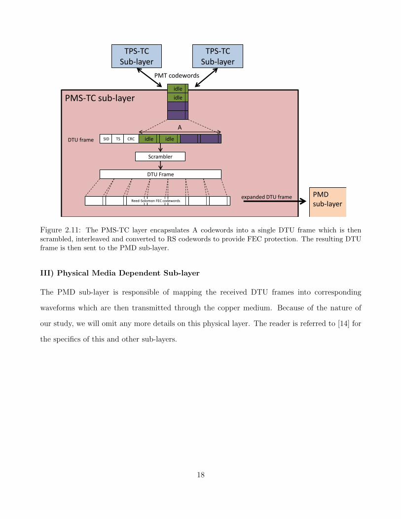
to the PMD sub-layer for transmission. This process is illustrated in Figure 2.11.
17
PMS-TC sub-layer
PMD sub-layer
TPS-TC Sub-layer
TPS-TC Sub-layer
idle
idle
PMT codewords
idle idle SID TS CRC DTU frame
Scrambler
DTU Frame
expanded DTU frame Reed-Solomon FEC codewords
A
Figure 2.11: The PMS-TC layer encapsulates A codewords into a single DTU frame which is thenscrambled, interleaved and converted to RS codewords to provide FEC protection. The resulting DTUframe is then sent to the PMD sub-layer.
III) Physical Media Dependent Sub-layer
The PMD sub-layer is responsible of mapping the received DTU frames into corresponding
waveforms which are then transmitted through the copper medium. Because of the nature of
our study, we will omit any more details on this physical layer. The reader is referred to [14] for
the specifics of this and other sub-layers.
18

Chapter 3: Reducing Memory Requirements on Drop-Point Devices
In order for hybrid PON/xDSL networks to become a feasible solution for future bandwidth
requirements, one of the main problems that must be addressed is reducing the power consump-
tion of the drop-point device [5]. There are several ways we can accomplish this task. One of
them is by reducing the design complexity of the drop-point device [3]. As it is now, the current
drop-point device oversees many tasks in the network. Some of these tasks include: keeping
track of the traffic management in order to ensure quality of service among the users. Also, the
drop-point device has to keep track of the buffer occupancy in order to prevent data loss. All
these tasks add complexity and increase the processing power required by the unit.
What we propose in our study is to reduce the memory complexity of the drop-point device
by applying back-pressure mechanisms towards the more resourceful OLT and CPE devices. By
using these back-pressure mechanisms we intend to limit the amount of packets being stored at
the drop-point device at any given time, thus reducing the total amount of memory required in
the unit. Doing this will reduce the number of transistors needed to fabricate such a device and
this will indirectly reduce the overall cost and power consumption of the unit.
In this chapter we analyze three methods by which we can reduce the buffer requirements in
the downstream and upstream directions. In section 3.1 we analyze a proposed mechanism to
reduce downstream memory utilization at the ONU by implementing a rate limiting device at
the OLT. In section 3.2 we first analyze the effects on the buffer by implementing a flow control
algorithm known as Input Buffer Limit. Then we consider the idea of extending the DBA
algorithms used by the OLT so that the MAC protocol at the PON coordinates the transmission
of both the ONU and the DSL sides of the drop-point device, we call this approach GATED flow
control.
3.1 Downstream buffering
In this section we analyze a method to limit the downstream buffer size at the drop-point by
limiting the maximum bitrate that can be delivered to the drop-point by the OLT at a given
19
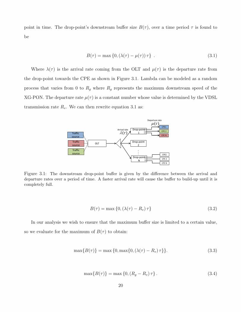
point in time. The drop-point’s downstream buffer size B(τ), over a time period τ is found to
be
B(τ) = max {0, (λ(τ)− µ(τ)) τ} . (3.1)
Where λ(τ) is the arrival rate coming from the OLT and µ(τ) is the departure rate from
the drop-point towards the CPE as shown in Figure 3.1. Lambda can be modeled as a random
process that varies from 0 to Rg where Rg represents the maximum downstream speed of the
XG-PON. The departure rate µ(τ) is a constant number whose value is determined by the VDSL
transmission rate Rv. We can then rewrite equation 3.1 as:
OLT
Drop-point 1
Drop-point N
Drop-point 2
. . .
CPE1
CPE N
CPE 2
CPE1
CPE N
CPE 2
Traffic source
Traffic source
Traffic source
)(
)(
Arrival rate
Departure rate
19
Figure 3.1: The downstream drop-point buffer is given by the difference between the arrival anddeparture rates over a period of time. A faster arrival rate will cause the buffer to build-up until it iscompletely full.
B(τ) = max {0, (λ(τ)−Rv) τ} (3.2)
In our analysis we wish to ensure that the maximum buffer size is limited to a certain value,
so we evaluate for the maximum of B(τ) to obtain:
max{B(τ)} = max {0,max{0, (λ(τ)−Rv) τ}}. (3.3)
max{B(τ)} = max {0, (Rg −Rv) τ} . (3.4)
20

From Equation (3.4) we can see that in order to bound the value of max{B(τ)} we have to
limit upper bound on the arrival rate.
3.1.1 Rate Limiting Device
A possible way by which we can limit the PON rate, and thus the arrival rate λ(τ), is by
implementing a rate limiting device, such as a traffic shaper, on the OLT side of the XG-PON
network as shown in Figure 3.2. A traffic shaper is a lossless rate limiting device whose purpose
is to limit the amount of bytes that flow through a transmission channel [15]. A traffic shaper has
two parameters: the bucket size b (in bytes) and the refill rate r (in bytes/sec). Whenever a
packet arrives to this device, a credit counter is checked to make sure enough credits are available
in the shaper. If the credit count is greater than or equal than the packet byte size, the packet
will then be forwarded to the intended destination, in this case the OLT transmission queue.
The credit counter will then be decreased by the packet’s byte size. In the case where the packet
size is bigger than the current credit counter, the packet will remain in a waiting queue until
enough credits are accumulated. The credits are refilled at a rate controlled by parameter r up
to the maximum bucket size b.
OLT
Optical Splitter
Drop-point 1
Drop-point N
1:N
Drop-point 2
. . .
Traffic for DP 1 Line 1
Traffic for DP 1 Line N
Traffic for DP 1 Line 2
Traffic Shaper
Traffic Shaper
Traffic Shaper
Figure 3.2: Each traffic shaper will only allow a limited amount of traffic to flow through the XG-PONwhich limits the arrival rate λ(τ) at the corresponding drop-point.
Given our traffic shaper, the number of bytes b(τ) that can flow through the traffic shaper in
any given time interval τ is given by:
b(τ) = b+ rτ (3.5)
21

The transmission rate r(τ) is then given by:
r(τ) =b(τ)
τ=b
τ+ r (3.6)
Since this rate will then be delivered through the XG-PON, equation (3.6) is also the arrival
rate at the drop-point, so λ(τ) = r(τ). Letting the refill rate r = Rv for our traffic shaper and
substituting back into (3.3) we obtain:
max{B(τ)} = max
{0,
(b
τ+Rv −Rv
)τ
}= max {0, b} = b (3.7)
From (3.7) we can see that the maximum buffer length at the drop-point is dependent on the
traffic shaper’s bucket size parameter b.
3.2 Upstream buffering
In this section we analyze two methods of reducing the drop-point’s memory requirements for
the upstream direction: Ethernet flow control and GATED flow control.
3.2.1 Ethernet Flow Control
Flow control, also known as congestion control [16] is a protocol or set of protocols designed to
keep the network from congesting by regulating the flow of packets [17]. The main functions of
flow control are: to prevent throughput degradation, ensure a fair allocation of resources, and
speed matching between users [17]. There are many kinds of flow control protocols which are
detailed in [17], however, in our study we will be dealing with a Network Access Flow Control type
known as Input Buffer Limit Scheme (IBLS) proposed in [18]. Network access flow control consists
on throttling the network inputs based on the measurements of internal network congestion.
More specifically, IBLS blocks the input traffic when certain buffer utilization thresholds are
reached. To do this, the buffer utilization is constantly being monitored as packets arrive. Once
the buffer size reaches a THRESHOLD value, the device sends a pause frame to the source
22

telling it to stop its transmission for PAUSE amount of time. This method allows a device
to apply back-pressure on the transmitting devices. Simulations done in [19] show that there
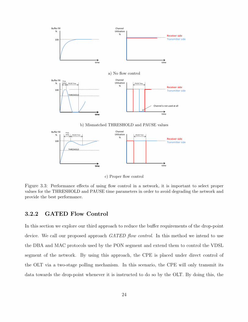
is an optimal buffer threshold that maximizes throughput for heavy traffic loads. Figure 3.3
illustrates the potential impact that flow control can have in a system. In Figure 3.3 a) we can
observe that applying no flow control to the network provides 100% transmission rates, however,
since the buffer is full all of the time, many packets are being dropped by the network and packet
retransmissions sent by the sources can cause a lot of congestion in the network. Eventually most
of the traffic flowing will only be due to the retransmissions and the actual throughput would
decrease drastically. Figure 3.3 b) shows the issues that may arise when selecting improper
THRESHOLD and PAUSE values. In this case, the THRESHOLD value has been set too high,
and because of the propagation delay, the PAUSE frame does not arrive to the sender before
the buffer becomes full. In this case, the PAUSE time was also set to a very long time causing
the network to be underutilized as can be seen on the right plot. Finally, Figure 3.3 c) shows
the proper use of the parameters in order to match the network’s propagation and transmission
rates. In this case, the buffer size oscillates within a given range, ideally close to 100%.
From the previous example we can conclude that several parameters like: transmission rate
and propagation delay should be carefully taken into account when selecting the proper THRESH-
OLD and PAUSE time values. In our simulations we first test several values for THRESHOLD
and PAUSE time in order to find the optimal conditions for our flow control algorithm.
In our application, this method of flow control, aims to reduce the minimum buffer size
needed at the drop-point device. Ethernet flow control is a well developed standard that does
this by signaling the DSL CPE unit to stop its transmission for a fixed amount of time after the
drop-point’s buffer reaches a certain threshold. Forcing the DSL CPE to stop its transmission
applies a back-pressure on the CPE. If desired, the CPE can then implement a similar approach
to signal the traffic source to stop its transmission as well. Eventually, the back-pressure will
reach the user’s equipment at the end-point of the netwrok. Pushing the traffic towards the user
is a simple way of reducing the memory needed in the network devices to store backlogged traffic.
23
time
Buffer fill %
100
time
Channel Utilization
% Receiver side Transmitter side
a) No flow control
time
Buffer fill %
time
100
THRESHOLD
PAUSE Time
Prop. delay
time
Channel Utilization
% Receiver side Transmitter side
PAUSE Time
Channel is not used at all
b) Mismatched THRESHOLD and PAUSE values
time
Buffer fill %
time
100
THRESHOLD
PAUSE Time
Prop. delay
time
Channel Utilization
% Receiver side Transmitter side
PAUSE Time
c) Proper flow control
Figure 3.3: Performance effects of using flow control in a network, it is important to select propervalues for the THRESHOLD and PAUSE time parameters in order to avoid degrading the network andprovide the best performance.
3.2.2 GATED Flow Control
In this section we explore our third approach to reduce the buffer requirements of the drop-point
device. We call our proposed approach GATED flow control. In this method we intend to use
the DBA and MAC protocols used by the PON segment and extend them to control the VDSL
segment of the network. By using this approach, the CPE is placed under direct control of
the OLT via a two-stage polling mechanism. In this scenario, the CPE will only transmit its
data towards the drop-point whenever it is instructed to do so by the OLT. By doing this, the
24

OLT can ensure that the drop-point will only receive data just in time before the ONU-side of
the drop-point retransmits the data towards the OLT. By implementing this semi cut-through
mechanism, we can ensure that only the data that is scheduled for transmission through the
PON will leave the CPE buffer instead of being stored at the drop-point as it would do in the
regular scenario.
A single drop-point device can have several point-to-point DSL connections which can all
transmit their upstream data in parallel. However, the order in which the OLT schedules their
transmission does have an effect in the polling time. We define the polling time as time interval
after the OLT started its transmission until the time when the first bit of data from the drop-point
is received by the OLT. In the following sections we illustrate our GATED flow control.
A. Polling time with a single attached CPE
OLT
Drop-
point
downstream(TX)
downstream(RX)
upstream(TX)
upstream(RX)
time
time Gt2 O
up
PR
G
C
Gt
PON
CPE downstream(RX)
upstream(TX)
time
up
SR
GC
downstream(TX)
upstream(RX) DSL
Ct
C2
Ot
up
SR
MTU
T
O
Figure 3.4: Polling time for a drop-point device with a single CPE attached.
We will first develop an expression for the polling time when there is only a single CPE
attached to the drop-point device as shown in Figure 3.4. In the figure we show the OLT
25
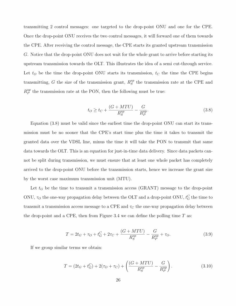
transmitting 2 control messages: one targeted to the drop-point ONU and one for the CPE.
Once the drop-point ONU receives the two control messages, it will forward one of them towards
the CPE. After receiving the control message, the CPE starts its granted upstream transmission
G. Notice that the drop-point ONU does not wait for the whole grant to arrive before starting its
upstream transmission towards the OLT. This illustrates the idea of a semi cut-through service.
Let tO be the time the drop-point ONU starts its transmission, tC the time the CPE begins
transmitting, G the size of the transmission grant, RupS the transmission rate at the CPE and
RupP the transmission rate at the PON, then the following must be true:
tO ≥ tC +(G+MTU)
RupS
− G
RupP
. (3.8)
Equation (3.8) must be valid since the earliest time the drop-point ONU can start its trans-
mission must be no sooner that the CPE’s start time plus the time it takes to transmit the
granted data over the VDSL line, minus the time it will take the PON to transmit that same
data towards the OLT. This is an equation for just-in-time data delivery. Since data packets can-
not be split during transmission, we must ensure that at least one whole packet has completely
arrived to the drop-point ONU before the transmission starts, hence we increase the grant size
by the worst case maximum transmission unit (MTU).
Let tG be the time to transmit a transmission access (GRANT) message to the drop-point
ONU, τO the one-way propagation delay between the OLT and a drop-point ONU, tCG the time to
transmit a transmission access message to a CPE and τC the one-way propagation delay between
the drop-point and a CPE, then from Figure 3.4 we can define the polling time T as:
T = 2tG + τO + tCG + 2τC +(G+MTU)
RupS
− G
RupP
+ τO. (3.9)
If we group similar terms we obtain:
T = (2tG + tCG) + 2(τO + τC) +
((G+MTU)
RupS
− G
RupP
). (3.10)
26

By inspecting equation (3.10) we observe that the first term corresponds to the time to
transmit the transmission access message across the PON and VDSL lines, the second term
represents the propagation delays between on the PON and VDSL segments respectively. Finally,
the third term represents the time for data to arrive just in time at the drop-point.
B. Polling time with two attached CPEs
OLT
Drop-
point
downstream(TX)
downstream(RX)
upstream(TX)
upstream(RX)
time Gt3
PON
CPE #1 downstream(RX)
upstream(TX)
time
downstream(TX)
upstream(RX) DSL #1
T
downstream(TX)
upstream(RX) DSL #2
CPE #2 downstream(RX)
upstream(TX)
up
SR
MTU
OC
Gt OC2
up
SR
MTU
Figure 3.5: Polling time for a drop-point device with two CPEs attached with parallel transmissioncapabilities.
We will now consider the case for two CPE’s attached to a single drop-point device, each
having independent point-to-point connections as shown in figure 3.5. In this case, the OLT
transmits 3 control messages: 1 for the drop-point ONU and 1 for each CPE. Each CPE starts
its transmission at the time indicated by the control message, However, the GRANT ordering does
have an impact of the total polling time. To show this, let G1 and G2 be the granted transmission
windows for CPE 1 and CPE 2 respectively and τ 1C and τ 2C be the one-way propagation delay
between the drop-point and CPE 1 and CPE 2 respectively. Similarly to the case of one CPE,
27

we can find the polling time to be:
T = (1+2)tG+tCG+2τO+max
(2τ 1C +
(G1 +MTU)
RupC
− G1
RupP
, 2τ 2C +(G2 +MTU)
RupC
− (G1 +G2)
RupP
).
(3.11)
In order to minimize (3.11) we have:
2τ 2C +G2
RupC
> 2τ 1C +G1
RupC
. (3.12)
So the CPE whose combined propagation delay and transmission time should be polled last.
C. Polling time with n attached CPEs
Finally, we consider the case where n CPEs are attached to a single drop-point device. General-
izing euqation (3.11) we find that,
T = (1 + n)tG + tCG + 2τO + maxi=1...n
(2τ iC +
(Gi +MTU)
RupC
−∑i
j=1Gj
RupP
). (3.13)
Similarly, to minimize (3.13) we need to order the CPE transmission in ascending order for
propagation and transmission time.
In our experiments we will compare the performance of extending the polling stage to the CPE
with and without the proposed optimization. We call these two methods GATED Flow Control
and GATED OPT Flow Control respectively. We will also compare the performance of the
traditional flow control using the Ethernet pauses after finding the optimal parameters for such
method. In order to get a good reference point on the performance of our proposed algorithms we
will also simulate the case were no flow control mechanism has been implemented. Our metrics
of interest are: the maximum buffer sizes per DSL line, the aggregate drop-point buffer size, the
observed queueing delays (DSL and PON) and the maximum achievable channel utilization.
28

Chapter 4: Performance Analysis
After formulating our hypothesis of how our proposed methods can limit the drop-point buffering
in both the downstream and upstream directions, we now need to verify the performance of
each algorithm. A physical implementation of the system is not a feasible way of testing the
performance of our methods due to the quantity and price of the equipment required. Instead,
we have designed two simulation engines that emulate the behavior of a real PON/VDSL access
network. The simulation engines were designed in the C programming language using a discrete
event simulation library [20]. The simulation engines will validate our mathematical analysis and
confirm the performance of our proposed methods.
In this chapter we present our experimental plan for our performance analysis and present
the results from our experiments. Section 4.1 presents the analysis related to the Downstream
performance while Section 4.2 covers the upstream performance analysis. The details regarding
the simulator implementation are omitted in this chapter but are later shown in Appendix A.
4.1 Downstream Performance
The goal of the downstream simulator is to verify that we can limit the downstream drop-point
buffer size by implementing a per DSL line traffic shaper at the OLT. The placement of the
traffic shapers for a single drop-point device is shown in Figure 4.1. To perform the analysis
we simulated several scenarios varying the amount of data generated by the traffic sources and
delivered to each DSL line. We also varied the parameters for the traffic shaper: bucket length
and fill rate. After observing the maximum buffer we can then asses the effectiveness of a traffic
shaper in limiting the drop-point’s downstream buffer size. According to our hypothesis, the
buffer size will not be affected by the traffic sources rate.
In our experiments we will simulate a system with 4 drop-point devices with a single VDSL line
connected to each device. The VDSL line bitrate has been configured to 75Mbit/sec. Our traffic
sources will generate data with a Self-Similar random distribution and a long term bitrate average
of {65, 70, 100} Mbit/sec. We have selected a Self-Similar distribution due to its similarity with
29

OLT Drop-point 1
CPE1
CPE N
CPE 2
Traffic source Traffic Shaper Splitter
Traffic source Traffic Shaper
Traffic source Traffic Shaper
VDSL line rate
Figure 4.1: A single traffic shaper device will be placed at the OLT for every CPE connected to eachdrop-point.
real Internet traffic. For each of the selected traffic bitrates, we will vary the parameters of the
traffic shapers to observe the effects that these have on the buffer length. According to our
analysis, only the bucket size parameter, b, should affect the maximum observed buffer size. In
our simulations we vary the traffic shapers’ fill rate to {70, 73, 74} Mbit/sec. It is important to
note that fill rate has to be less than the VDSL rate in order to prevent a buffer overflow. For
our bucket size parameter, we have selected the following values: {10, 50, 100} Kbytes.
In our simulator we made two important assumptions regarding the behavior of the OLT and
drop-point systems. First, we assumed a PHY frame is completely assembled from the arriving
traffic packets before it is transmitted to the drop-points. Secondly, we assumed that the drop-
point will not forward any packets to the VDSL queues until a complete PHY frame has been
received from the OLT.
Table 4.1: Downstream maximum recorded drop-point buffer lengths.
Fill Rate (Mbit/sec) Bucket Size (Kbytes)Drop-point Buffer (bytes)
Traffic Source Rate (Mbit/sec)65 75 100
7010 11086 11086 1077650 51080 51064 50024100 101058 101066 99800
7310 11352 11568 1110450 51352 51350 50824100 101118 101310 100586
7410 63080 96032 ∞50 107780 176288 ∞100 183424 265938 ∞
Our observations are presented in Table 4.1. Columns 3, 4 and 5 in the table show the max-
30

imum buffer lengths recorded for the different generated traffic bitrates {65, 70, 100} Mbit/sec
respectively. As we can observe, for any selected fill rate and bucket size configuration the buffer
size of the drop-point is independent of the traffic bitrate. Without a traffic shaper, higher traffic
bitrates would result in larger buffer sizes, however, this is clearly not the case. On the contrary,
we can observe that at higher traffic rates, the buffer size actually diminishes. This occurs be-
cause at higher traffic rates, the traffic shaper credits are less likely to accumulate due to the
more frequent data arrival. Secondly, we observe that selecting a fill rate of 74Mbit/sec causes
the drop-point buffers to overflow. Even though the departure rate of the VDSL lines is set to
75Mbit/sec, this value does not consider the overhead bytes added due to the VDSL2 protocol
encapsulation. This overhead causes the effective VDSL bitrate to be less than 74Mbit/sec and
thus causes an infinite buffer to accumulate of time. Finally, we can also observe that higher fill
rates lead to a larger recorded buffer size. This is a discrepancy from our analysis in Chapter 3
which we will explain as follows. As we mentioned before, our simulator engine assumes that a
PHY frame is completely assembled before it is transmitted to the drop-points, this is shown in
Figure 4.2.
OLT
Drop-point N
PHY frame PHY frame
PHY frame PHY frame
125 µsec
time
Figure 4.2: During the 125 µsec transmission period, packets arriving from the traffic shapers areencapsulated into the next PHY frame.
This “wait to assemble” period allows the traffic shaper to transmit more bytes during this
period as more credits are constantly being generated. Due to this behavior the maximum buffer
size we observe is now given by:
max{B(τ)} = b+ r0τ (4.1)
31

This equation has an extra term as compared to Equation (3.7). Recall that the XG-PON
protocol specifies a constant PHY frame duration of τ = 125 µsec. Despite the additional term
in the equation, the obtained buffer size can still be bounded by the traffic shaper by configuring
the b and r0 parameter values.
4.2 Upstream Performance
The goal of the upstream simulations is to asses the performance of the developed flow control
mechanisms compared to the case where no flow control mechanism has been implemented. We
will measure the performance of each algorithm with respect following criteria:
• PON queueing delay: defined as the amount of time a packet has to wait at the
drop-point before it is transmitted towards the OLT.
• DSL queueing delay: defined as the time a packet has to wait at the CPE before it
is transmitted through the VDSL line and received by the drop-point device.
• Maximum per DSL line buffer length: this is the maximum observed buffer length
for a single DSL line. This value is obtained by comparing all single DSL line buffers from
all the drop-points: max (Bi,j(t)).
• Maximum drop-point aggregate buffer length: this is the maximum observed
buffer length for all DSL lines in a single drop-point. This value is obtained by comparing
the total buffer length of all the DSL lines within a drop-point device: max(∑DSL
j=1 Bi,j(t)).
• Channel utilization: data bitrate that can be transmitted in a channel with trans-
mission rate R. In most cases the actual throughput is less than the transmission rate due
to the overhead added in the encapsulation.
We will divide our upstream performance analysis into three main steps. In the first step
we will measure the system performance without applying any of our proposed flow control
algorithms, this test will serve as the control case for future comparison. Next we will find
32

the optimal parameters for the Ethernet flow control mechanism as described in Chapter 3.
Finally, we will compare the performance of the three flow control algorithms using different
PON configurations, such as varying the cycle length or the DBA algorithm.
4.2.1 Step 1: Control case
In this step we analyze the performance of the system without any flow control algorithm by
recording the maximum per DSL line buffer length. To prevent any packet loss in this experiment
we will configure our drop-points to have an infinite size buffer. Next, we will observe the packet
loss rates that would occur when using the more realistic {10 KB, 50 KB, 100 KB} per DSL
buffer sizes.
We have configured our simulation engine to simulate a network with a realistic x8 over-
subscription rate. To attain this over-subscription rate we will have 32 drop-points with 8 VDSL
lines attached for a total of 256 VDSL lines. Each VDSL line has a codeword generation rate of
75 Mbit/sec. Each of the drop-points will have a random propagation delay between 2.5 µsec
and 100 µsec, which corresponds to a realistic range of 500 m to 20 km away from the OLT. Our
PON segment has been configured, according to the XG-PON standard, to have a transmission
rate of 2.488 Gbit/sec. Without loss of generality we have selected an {Online, Excess} DBA
algorithm for our OLT scheduler. In this simulation we will vary the packet arrival rate by using
a Self-Similar traffic generator connected to each CPE line independently. The long-term average
packet bitrate will vary in our simulations from {20%, 30%,..,90%} the PON transmission rate
for each of the packet generators. A summary of the simulation configurations is shown in Table
4.2
We will also simulate a similar network using the G.Fast protocol instead of the VDSL2
protocol. In order to keep the over-subscription rate at x8, we will only simulate 16 drop-point
devices with 8 G.Fast DSL lines each, for a total of 128 lines. Each G.Fat line will have a
codeword generation rate of 300 Mbit/sec. The Time Division Duplexing on the G.Fast has
been configured to a 50%-50% upstream/downstream transmission. The rest of the parameters
33

Table 4.2: Configuration parameters for the upstream simulation plan, step 1.
Parameter ValueSimulation Run time 30 million packetsTraffic Source Distribution Self-SimilarTraffic Source Load (rate) {20%, 30%, ..., 90%} of 2.488 Gbit/secNumber of Drop-points 32VDSL lines per drop-point 8VDSL codeword bitrate 75 Mbit/secDrop-point Buffer size {10 KB, 50 KB, 100 KB, ∞}Drop-point-OLT Propagation delay N (2.5 µsec, 100 µsec)Flow Control Algorithm NonePON bitrate 2.488 Gbit/secGuard time 30 nsecOLT DBA algorithm {Online, Excess}
have been left as in the previous case.
Our simulation results are presented in Table 4.3 and Table 4.4 for maximum buffer length
and packet loss respectively. As we can observe in Table 4.3, for the VDSL2 protocol a 50 KB
buffer would be enough to for cases is which the total traffic load is less than 80 %. In the case
of G.Fast, we require a 100 KB buffer for traffic loads up to 70 %. Despite the similar over-
subscription rate for both systems, we observe that the VDSL2 provides a better performance in
reducing the maximum buffer length. This occurs because G.Fast uses Time Division Duplexing
which periodically disables the upstream transmission. During the OFF period, the buffer at
the CPE will accumulate data coming from the traffic generators and once the ON time starts,
the CPE will burst this data towards the drop-point. This case is similar to our “stop and wait”
observations for the downstream traffic shaper discussed in section 4.1. Finally, we observe that
traffic loads greater than 80 % will require some sort of Flow Control mechanism in order to
bound the maximum buffer length.
From Table 4.4 we observe that a providing a buffer of 10 KB is completely unacceptable
as the observed packet losses are considerably high. Using a 100 KB buffer would provide a
somewhat acceptable packet loss rate less than 3 % for both the VDSL2 and G.Fast protocols.
However, we expect these packet loss values to increase considerably as get generate higher traffic
34

Table 4.3: Maximum Buffer Length with no Flow Control
LoadVDSL2 G.Fast TDD
per DSL buffer Aggregate buffer per DSL buffer Aggregate buffer
0.90 9382 KB 20832 KB 7465 KB 14149 KB
0.80 19 KB 56 KB 298 KB 623 KB
0.70 13 KB 37 KB 40 KB 104 KB
0.60 9 KB 33 KB 30 KB 88 KB
0.50 9 KB 30 KB 22 KB 81 KB
0.40 9 KB 28 KB 22 KB 74 KB
0.30 8 KB 26 KB 22 KB 70 KB
0.20 - - 22 KB 61 KB
loads conditions as we do in the last part of this experimental plan.
Table 4.4: Maximum Loss Rates with no Flow Control
Queue Size LoadVDSL2 G.Fast TDD
Packet Loss Rate Byte Loss Rate Packet Loss Rate Byte Loss Rate
10 KB 0.8 10.0 % 15.8 % 26.9 % 37.7 %
50 KB 0.8 3.20 % 3.40 % 2.23 % 2.31 %
100 KB 0.8 2.89 % 3.07 % 1.94 % 2.08 %
35

4.2.2 Step 2: Optimal point for Ethernet flow control
As discussed in Section 3.2.1 it is important to find the optimal value for the flow control
THRESHOLD and PAUSE time parameters. In this section we design an experimental plan to
find this optimal point.
Our system parameters are similar to step 1. In this case the will use a constant traffic load of
80% the PON transmission rate. We have selected this value as this seems to be the point where
buffers start saturating as observed in the previous section. For this study we will test several
values for the THRESHOLD and PAUSE time parameters and evaluate which configuration
provides the lowest packet loss. We summarize our system configurations in Table 4.5.
Table 4.5: Configuration parameters for the upstream simulation plan, step 2.
Parameter ValueSimulation Run time 30 million packetsTraffic Source Distribution Self-SimilarTraffic Source Load (rate) 80% of 2.488 Gbit/secNumber of Drop-points 32 (16 for G.Fast)VDSL lines per drop-point 8VDSL codeword bitrate 75 Mbit/sec (300 for G.Fast)Drop-point Buffer size {10 KB, 50 KB, 100 KB}Drop-point-OLT Propagation delay N (2.5 µsec, 100 µsec)Flow Control Algorithm Ethernet Flow Control
PAUSE time {2, 3, 4, 5} millisecTHRESHOLD trigger {30, 40, 50, 60} %
PON bitrate 2.488 Gbit/secGuard time 30 nsecOLT DBA algorithm {Online, Excess}
Our simulation results are shown in Table 4.6 and are presented graphically in Figure 4.3.
The table presents the observed packet loss rates for both the VDSL and G.Fast simulations
using the different combinations for THRESHOLD and PAUSE time parameters. We observe
that a buffer size of 10 KB is too small to prevent any significant packet loss regardless of the flow
control configuration used. The reason for this is that even when the pause signal is triggered
at 30% the buffer capacity, only 7 KB of memory will be available to store the arriving traffic
36

before the CPE receives the PAUSE frame and stops its transmission. At the current VDSL
transmission bitrates, 7 KB of data correspond to roughly 747 µsec of transmission time. This is
equivalent to roughly 6 Maximum Size Ethernet frames, as a result, the packet losses are quite
high. For the 50 KB and 100 KB buffer sizes, we observe that for most combinations of flow
control parameters yield a packet loss of less than 1 %. In many cases, complete packet loss can
be prevented with either buffer size.
For the 100 KB buffer case, we observe that a THRESHOLD value of 30% can prevent
complete packet loss and even at 40%, the packets losses are very small. This occurs because
after the PAUSE signal is sent, the buffer will have close to 7.466 msec (70 KB) worth of space
to absorb the data that is still being transmitted. Since data is scheduled to leave the drop-point
every cycle length, 2 msec in our simulations, this is more than enough time to prevent packet
losses.
It is important to note that in our simulation engine, we considered the propagation delay
between the drop-points and CPEs negligible. However, in systems where the propagation time
becomes more significant, a larger buffer size will be needed to absorb all of the transmitted data
before the PAUSE frame reaches the CPE. If buffer sizes are left as is, we would expect packet
losses to increase. Another possible solution is to decrease the THRESHOLD value to trigger
the PAUSE frame at an earlier stage.
37

Threshold 30% Threshold 40% Threshold 50% Threshold 60%
6
8
10
12
14
2.0 msec 2.5 msec 3.0 msec 3.5 msec 4.0 msec 4.5 msec 5.0 msec
% P
ack
et
Lo
ss
PAUSE time (seconds)
Threshold 30% Threshold 40% Threshold 50% Threshold 60%
10
15
20
25
30
35
2.0 msec 2.5 msec 3.0 msec 3.5 msec 4.0 msec 4.5 msec 5.0 msec
% P
ack
et
Lo
ss
PAUSE time (seconds)
a) VDSL2 - 10 KB buffer b) G.Fast - 10 KB buffer
Threshold 30% Threshold 40% Threshold 50% Threshold 60%
0
0.5
1
1.5
2
2.5
3
2.0 msec 2.5 msec 3.0 msec 3.5 msec 4.0 msec 4.5 msec 5.0 msec
% P
ack
et
Lo
ss
PAUSE time (seconds)
Threshold 30% Threshold 40% Threshold 50% Threshold 60%
0
0.2
0.4
0.6
0.8
1
1.2
2.0 msec 2.5 msec 3.0 msec 3.5 msec 4.0 msec 4.5 msec 5.0 msec
% P
ack
et
Lo
ss
PAUSE time (seconds)
c) VDSL2 - 50 KB buffer d) G.Fast - 50 KB buffer
Threshold 30% Threshold 40% Threshold 50% Threshold 60%
0
0.2
0.4
0.6
0.8
1
2.0 msec 2.5 msec 3.0 msec 3.5 msec 4.0 msec 4.5 msec 5.0 msec
% P
acket
Loss
PAUSE time (seconds)
Threshold 30% Threshold 40% Threshold 50% Threshold 60%
0
0.2
0.4
0.6
0.8
1
1.2
1.4
2.0 msec 2.5 msec 3.0 msec 3.5 msec 4.0 msec 4.5 msec 5.0 msec
% P
acket
Loss
PAUSE time (seconds)
e) VDSL2 - 100 KB buffer f) G.Fast - 100 KB buffer
Figure 4.3: Packet Loss Rate at 80% channel load.
38

Table 4.6: Packet Loss observations at 80% traffic loadBuffer Cap. Threshold Pause Time Packet Loss Rate Packet Loss Rate
(KB) % (msec) % %
10
30
2ms 7.36 17.633ms 11.09 22.444ms 12.75 33.435ms 14.21 34.79
40
2ms 7.01 16.853ms 8.55 19.814ms 11.26 22.995ms 12.19 29.38
50
2ms 7.62 16.763ms 8.69 18.904ms 10.52 22.725ms 13.57 25.13
60
2ms 10.34 15.203ms 11.29 17.574ms 12.58 19.405ms 14.2 22.69
50
30
2ms 0.85 0.7013ms 0.372 0.1624ms 0.082 05ms 0.15 0.0024
40
2ms 1.04 0.7573ms 0.44 0.1194ms 0.17 0.0215ms 0.32 0.0194
50
2ms 1.72 0.7823ms 1.08 0.1244ms 0.65 0.0285ms 0.47 0.043
60
2ms 2.14 0.7723ms 1.9 0.1424ms 1.85 0.1355ms 1.9 0.071
100
30
2ms 0 0.913ms 0 0.0744ms 0 05ms 0 0
40
2ms 0 0.863ms 0.005 0.0944ms 0.003 05ms 0.003 0
50
2ms 0.18 1.023ms 0.137 0.1674ms 0.142 05ms 0.018 0
60
2ms 0.455 1.063ms 0.42 0.214ms 0.25 0.01785ms 0.5 0
39

4.2.3 Step 3: Performance Comparison between flow control mecha-
nisms
In this section we will observe the performance of the various flow control algorithms proposed
in chapter 3. We are mainly concerned with understanding the behavior of the packet delay and
the maximum buffer occupancy for the various mechanisms under different operating conditions.
Table 4.7 shows the configuration parameters used. In these experiments we will test the per-
formance of the four algorithms using {Online, Excess} and {Online, Limited} DBA algorithms
and several cycle lengths, {3 msec, 4 msec, 8 msec}, for the PON segment. For this part of the
analysis we will not use G.Fast because the GATED OPT mechanism has not yet been imple-
mented and it is part of our future work. For the case of Ethernet PAUSE Flow control, we
will be using the optimal parameter of 30 % THRESHOLD and 2 msec PAUSE time found in
Section 4.2.2.
Table 4.7: Configuration parameters for the upstream simulation plan, step 3.
Parameter ValueSimulation Run time 30 million packetsTraffic Source Distribution Self-SimilarTraffic Source Load (rate) {74%, 76%, ..., 88%} of 2.488 Gbit/secNumber of Drop-points 32VDSL lines per drop-point 8VDSL codeword bitrate 75 Mbit/sec (300 for G.Fast)Drop-point Buffer size 100 KB per DSL lineDrop-point-OLT Propagation delay N (2.5 µsec, 100 µsec)Flow Control Algorithm No Flow Control
Ethernet PAUSE Flow Control (30%, 2 msec)GATED Flow ControlGATED OPTimized Flow Control
PON bitrate 2.488 Gbit/secGuard time 30 nsecPON cycle length {3 msec, 4 msec, 8 msec}OLT DBA algorithm {Online, Excess}
{Online, Limited}
The results of this section are somewhat more extensive than in the previous cases. To
40

make the analysis more organized we will subdivide the results according to the performance
metric being evaluated in each case. We present our observations for each metric in the following
subsections.
4.2.3.1) PON queueing delay
In this section we analyze the performance of our algorithms with respect to the PON queueing
delay. As stated previously, this delay corresponds to the time interval after a data packet
arrives to an drop-point queue and the moment this same packet is transmitted through the PON
segment as the head-of-the-line packet. Our measurement observations are shown in Figure 4.4.
In the figure, the plots on the left column: a), c) and e) correspond to the observations using
an {Online, Excess} DBA algorithm, while the plots on the right column: b), d) and f) use an
{Online, Limited} DBA. Plots in similar rows: (a, b), (c, d) and (e, f) compare the results using
3 msec, 4 msec and 8 msec cycle lengths respectively.
In these plots we observe that the cycle length has a significant influence on the GATED flow
control algorithms, while the PAUSE and no flow control algorithms seem to be unaffected by this
configuration. We also observe that the cycle length has a big influence on the maximum channel
utilization that can be achieved with the PAUSE and no flow control algorithms. This observation
can be made by looking at the point where the delay curve starts growing exponentially. For
example, in the case of plot a), we see that at around 84 % traffic load the delay values start
increasing considerably, so we say that there is a 84 % channel capacity. We observe that PAUSE
flow control has a slightly smaller channel capacity, and thus a smaller delay, compared to no
flow control, however, this differences diminishes as we increase the cycle length.
When comparing the performance based on the DBA algorithm, we observe that an {Online,
Limited} scheme provides slightly smaller delays for the GATED algorithms, while the opposite
is true for the PAUSE and no flow control algorithms. In either case, we cannot observe any
significant change in the channel utilization in either DBA algorithm.
As it would be expected, the GATED OPTimized algorithm has a better performance than
41

Gated/Opt Flow CtrlGated Flow CtrlPAUSE Flow CtrlNo Flow Ctrl
400.0 usec
600.0 usec
800.0 usec
1.0 msec
1.2 msec
1.4 msec
1.6 msec
1.8 msec
2.0 msec
0.74 0.76 0.78 0.8 0.82 0.84 0.86 0.88
del
ay (
in s
eco
nd
s)
load (in fraction of 2.488 Gbps)
Gated/Opt Flow CtrlGated Flow CtrlPAUSE Flow CtrlNo Flow Ctrl
400.0 usec
600.0 usec
800.0 usec
1.0 msec
1.2 msec
1.4 msec
1.6 msec
1.8 msec
2.0 msec
0.74 0.76 0.78 0.8 0.82 0.84 0.86 0.88
del
ay (
in s
eco
nd
s)
load (in fraction of 2.488 Gbps)
a) {Online, Excess} 3 msec cycle length b) {Online, Limited} 3 msec cycle length
Gated/Opt Flow CtrlGated Flow CtrlPAUSE Flow CtrlNo Flow Ctrl
400.0 usec
600.0 usec
800.0 usec
1.0 msec
1.2 msec
1.4 msec
1.6 msec
1.8 msec
2.0 msec
0.74 0.76 0.78 0.8 0.82 0.84 0.86 0.88
del
ay (
in s
eco
nd
s)
load (in fraction of 2.488 Gbps)
Gated/Opt Flow CtrlGated Flow CtrlPAUSE Flow CtrlNo Flow Ctrl
400.0 usec
600.0 usec
800.0 usec
1.0 msec
1.2 msec
1.4 msec
1.6 msec
1.8 msec
2.0 msec
0.74 0.76 0.78 0.8 0.82 0.84 0.86 0.88
del
ay (
in s
eco
nd
s)
load (in fraction of 2.488 Gbps)
c) {Online, Excess} 4 msec cycle length d) {Online, Limited} 4 msec cycle length
Gated/Opt Flow CtrlGated Flow CtrlPAUSE Flow CtrlNo Flow Ctrl
400.0 usec
600.0 usec
800.0 usec
1.0 msec
1.2 msec
1.4 msec
1.6 msec
1.8 msec
2.0 msec
2.2 msec
0.74 0.76 0.78 0.8 0.82 0.84 0.86 0.88
del
ay (
in s
econ
ds)
load (in fraction of 2.488 Gbps)
Gated/Opt Flow CtrlGated Flow CtrlPAUSE Flow CtrlNo Flow Ctrl
400.0 usec
600.0 usec
800.0 usec
1.0 msec
1.2 msec
1.4 msec
1.6 msec
1.8 msec
2.0 msec
0.74 0.76 0.78 0.8 0.82 0.84 0.86 0.88
del
ay (
in s
econ
ds)
load (in fraction of 2.488 Gbps)
e) {Online, Excess} 8 msec cycle length f) {Online, Limited} 8 msec cycle length
Figure 4.4: PON queueing Delays
the simpler GATED flow control. Likewise, we observe that the PAUSE flow control is slightly
slower than the regular no flow control algorithm. We observe that for lower traffic loads, PAUSE
and no flow control algorithm out perform our proposed GATED algorithms. However, as the
traffic load increases, the GATED flow control algorithms provide a consistent stable delay that
ends up performing better than the counterpart algorithms. This behavior is not intuitive as the
main purpose of the GATED algorithm was to provide a cut-through service at the drop-point
and thus provide a minimal delay at this stage. To understand this behavior we will refer to
Figure 4.5 that shows the PON segment queueing delay distribution for the simulation case of
42

{Online, Limited} and 3 msec cycle length. Plot a) shows the majority of the weight of the
distribution and plot b) shows the tail of the distribution appropriately zoomed to see the detail.
GATED/OPT Flow Ctrl GATED Flow Ctrl PAUSE Flow Ctrl No Flow Ctrl
0
0.05
0.1
0.15
0.2
0.25
0.3
0.35
0.4
0 100 200 300 400 500 600 700 800
Pro
bab
ilit
y
delay value (in usec)
GATED/OPT Flow Ctrl GATED Flow Ctrl PAUSE Flow Ctrl No Flow Ctrl
0
0.0005
0.001
0.0015
0.002
0.0025
0.003
1.0 1.5 2.0 2.5 3.0 3.5 4.0
Pro
bab
ilit
y
delay value (in msec)
a) Most of the distribution b) Tail of the distribution (zoomed in)
Figure 4.5: Histogram of PON queue delay values for an average presented load of 74% (of2.488 Gbit/sec). The values are shown for the simulation case of {Online, Limited} and 3 mseccycle length
If we recall from our analysis in Chapter 3, Equation 3.8 shows that packets from the DSL
must arrive a maximum transmission time unit (MTU) earlier to ensure that a full packet is
always received before it can be transmitted upstream on the PON. For an MTU of 1518 bytes
and a DSL upstream transmission rate of 75 Mbit/sec, this time is approximately 162 µsec. We
can see from the delay distribution that there is some significant weight around this value for the
GATED flow control mechanisms. There is also some significant weight around double this value
for the GATED flow control mechanisms. Finally, there is significant weight in the tail. This
tail weight, inexistent for the PAUSE an no flow control, is the reason why the PON segment
delay is larger for the GATED flow control mechanisms. This tail weight occurs because of an
idiosyncrasy of the GATED flow control mechanism. With the GATED flow control mechanism
a transmission GRANT must be generated separately for the PON segment and for each of the
DSL segments. With the different overheads on each segment (e.g., XGEM frame overhead on
XG-PON and PTM Codeword/DTU frame overhead on VDSL), the transmission grant sizes will
not be identical.
The result of this grant size mismatch is that an Ethernet frame that is accounted for in
the XG-PON grant may not be fully accounted for in the DSL grant. In this case some of the
43

XG-PON capacity is wasted and a frame will sit partially received at the drop-point. In the next
grant cycle, that frame is completely received and is transmitted a granting cycle later. However,
this extra bytes consume the space of one or more Ethernet frames in the new XG-PON grant
forcing some frames to be serviced in the next grant cycle. To mitigate this, the drop-point
should report any residual Ethernet data left over. This report from the drop-point is considered
together with the report from the DSL CPE when determining the next drop-point transmission
grant.
4.2.3.2) DSL delay
In this section we analyze the performance of our algorithms with respect to the DSL delay. As
stated previously, this delay corresponds to the time interval after a data packet arrives to an
CPE queue and the moment this same packet is received at the drop-point DSL queue. Our
measurement observations are shown in Figure 4.6. The organization of this figure is similar to
the one shown in the previous section.
As we can see from the graphs, the DSL delay of our GATED algorithms is always bigger
than the delay for PAUSE and no flow control. This is an expected result as the purpose of our
GATED algorithms was to have packets wait at the CPE rather than wait at the drop-point’s
queue. We can observe that the cycle length configuration has a significant effect on the channel
utilization for the GATED algorithms, contrary to the PON queue delay where the channel
utilization was observed at the PAUSE and no flow control algorithms. As it would be expected,
the DSL delay is unaffected by the type of DBA algorithm used in the simulations.
4.2.3.3) Maximum buffer Length
In this section we analyze the performance of our algorithms with respect to the maximum
buffer lengths. We will first analyze the case of per DSL buffer lengths and then proceed to the
drop-point aggregate buffer lengths. Our measurement observations for a per DSL buffer length
are shown in Figure 4.7. Figure 4.8 shows the measurement observations for the drop-point
aggregate buffer lengths. The organization of these figures is similar to the ones shown in the
44

Gated/Opt Flow CtrlGated Flow CtrlPAUSE Flow CtrlNo Flow Ctrl
5.0 msec
10.0 msec
15.0 msec
20.0 msec
25.0 msec
30.0 msec
35.0 msec
40.0 msec
45.0 msec
50.0 msec
0.74 0.76 0.78 0.8 0.82 0.84 0.86 0.88
del
ay (
in s
eco
nd
s)
load (in fraction of 2.488 Gbps)
Gated/Opt Flow CtrlGated Flow CtrlPAUSE Flow CtrlNo Flow Ctrl
5.0 msec
10.0 msec
15.0 msec
20.0 msec
25.0 msec
30.0 msec
35.0 msec
40.0 msec
45.0 msec
50.0 msec
0.74 0.76 0.78 0.8 0.82 0.84 0.86 0.88
del
ay (
in s
eco
nd
s)
load (in fraction of 2.488 Gbps)
a) {Online, Excess} 3 msec cycle length b) {Online, Limited} 3 msec cycle length
Gated/Opt Flow CtrlGated Flow CtrlPAUSE Flow CtrlNo Flow Ctrl
5.0 msec
10.0 msec
15.0 msec
20.0 msec
25.0 msec
30.0 msec
35.0 msec
40.0 msec
45.0 msec
50.0 msec
0.74 0.76 0.78 0.8 0.82 0.84 0.86 0.88
del
ay (
in s
eco
nd
s)
load (in fraction of 2.488 Gbps)
Gated/Opt Flow CtrlGated Flow CtrlPAUSE Flow CtrlNo Flow Ctrl
5.0 msec
10.0 msec
15.0 msec
20.0 msec
25.0 msec
30.0 msec
35.0 msec
40.0 msec
45.0 msec
50.0 msec
0.74 0.76 0.78 0.8 0.82 0.84 0.86 0.88
del
ay (
in s
eco
nd
s)
load (in fraction of 2.488 Gbps)
c) {Online, Excess} 4 msec cycle length d) {Online, Limited} 4 msec cycle length
Gated/Opt Flow CtrlGated Flow CtrlPAUSE Flow CtrlNo Flow Ctrl
5.0 msec
10.0 msec
15.0 msec
20.0 msec
25.0 msec
30.0 msec
35.0 msec
40.0 msec
45.0 msec
50.0 msec
0.74 0.76 0.78 0.8 0.82 0.84 0.86 0.88
del
ay (
in s
econ
ds)
load (in fraction of 2.488 Gbps)
Gated/Opt Flow CtrlGated Flow CtrlPAUSE Flow CtrlNo Flow Ctrl
5.0 msec
10.0 msec
15.0 msec
20.0 msec
25.0 msec
30.0 msec
35.0 msec
40.0 msec
45.0 msec
50.0 msec
0.74 0.76 0.78 0.8 0.82 0.84 0.86 0.88
del
ay (
in s
econ
ds)
load (in fraction of 2.488 Gbps)
e) {Online, Excess} 8 msec cycle length f) {Online, Limited} 8 msec cycle length
Figure 4.6: DSL Queueing Delays
previous sections.
As we can observe from Figure 4.7, increasing the cycle length in the PON causes an increase
in the buffer size for GATED algorithms. In the case of plot e) the maximum buffer required
is over 100 KB. Using an {Online, Limited} DBA algorithm reduces the buffer requirements for
all algorithms compared to using an {Online, Excess} DBA. As we can observe, PAUSE and no
flow control algorithms require a smaller buffer compared to the GATED algorithms for small
traffic loads. However, as the traffic load increases, the GATED flow control algorithms provide
a stable buffer occupancy compared to the PAUSE and no flow control algorithms which have
45

Gated/Opt Flow CtrlGated Flow CtrlPAUSE Flow CtrlNo Flow Ctrl
10000
20000
30000
40000
50000
60000
70000
80000
90000
100000
0.74 0.76 0.78 0.8 0.82 0.84 0.86 0.88
Max
. B
uff
er L
en.
(in
by
tes)
load (in fraction of 2.488 Gbps)
Gated/Opt Flow CtrlGated Flow CtrlPAUSE Flow CtrlNo Flow Ctrl
10000
20000
30000
40000
50000
60000
70000
80000
90000
100000
0.74 0.76 0.78 0.8 0.82 0.84 0.86 0.88
Max
. B
uff
er L
en.
(in
by
tes)
load (in fraction of 2.488 Gbps)
a) {Online, Excess} 3 msec cycle length b) {Online, Limited} 3 msec cycle length
Gated/Opt Flow CtrlGated Flow CtrlPAUSE Flow CtrlNo Flow Ctrl
10000
20000
30000
40000
50000
60000
70000
80000
90000
100000
0.74 0.76 0.78 0.8 0.82 0.84 0.86 0.88
Max
. B
uff
er L
en.
(in
by
tes)
load (in fraction of 2.488 Gbps)
Gated/Opt Flow CtrlGated Flow CtrlPAUSE Flow CtrlNo Flow Ctrl
10000
20000
30000
40000
50000
60000
70000
80000
90000
100000
0.74 0.76 0.78 0.8 0.82 0.84 0.86 0.88
Max
. B
uff
er L
en.
(in
by
tes)
load (in fraction of 2.488 Gbps)
c) {Online, Excess} 4 msec cycle length d) {Online, Limited} 4 msec cycle length
Gated/Opt Flow CtrlGated Flow CtrlPAUSE Flow CtrlNo Flow Ctrl
10000
20000
30000
40000
50000
60000
70000
80000
90000
100000
0.74 0.76 0.78 0.8 0.82 0.84 0.86 0.88
Max
. B
uff
er L
en.
(in
by
tes)
load (in fraction of 2.488 Gbps)
Gated/Opt Flow CtrlGated Flow CtrlPAUSE Flow CtrlNo Flow Ctrl
10000
20000
30000
40000
50000
60000
70000
80000
90000
100000
110000
0.74 0.76 0.78 0.8 0.82 0.84 0.86 0.88
Max
. B
uff
er L
en.
(in
by
tes)
load (in fraction of 2.488 Gbps)
e) {Online, Excess} 8 msec cycle length f) {Online, Limited} 8 msec cycle length
Figure 4.7: Maximum per DSL buffer Length
an unbounded buffer growth. If we were to observe the buffer size at the CPEs, we would see a
large buffer size for the GATED algorithms as these algorithms were designed to back-pressure
the data away from the drop-point into the CPEs.
As we can see in Figure 4.8, the aggregate drop-point maximum buffer occupancies is about
the same for the GATED flow control algorithms compared to the per DSL buffer length seen
in Figure 4.7. However, for the PAUSE and no flow control algorithms the aggregate drop-point
maximum buffer occupancy is a multiple of the per DSL queue maximum buffer occupancy. We
observe this advantageous behavior with the GATED flow control mechanisms because these
46
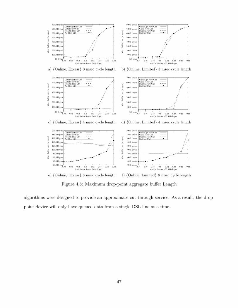
Gated/Opt Flow CtrlGated Flow CtrlPAUSE Flow CtrlNo Flow Ctrl
0.0 bytes
100.0 kbytes
200.0 kbytes
300.0 kbytes
400.0 kbytes
500.0 kbytes
600.0 kbytes
700.0 kbytes
800.0 kbytes
0.74 0.76 0.78 0.8 0.82 0.84 0.86 0.88
Max
. B
uff
er L
en.
(in
by
tes)
load (in fraction of 2.488 Gbps)
Gated/Opt Flow CtrlGated Flow CtrlPAUSE Flow CtrlNo Flow Ctrl
0.0 bytes
100.0 kbytes
200.0 kbytes
300.0 kbytes
400.0 kbytes
500.0 kbytes
600.0 kbytes
700.0 kbytes
800.0 kbytes
0.74 0.76 0.78 0.8 0.82 0.84 0.86 0.88
Max
. B
uff
er L
en.
(in
by
tes)
load (in fraction of 2.488 Gbps)
a) {Online, Excess} 3 msec cycle length b) {Online, Limited} 3 msec cycle length
Gated/Opt Flow CtrlGated Flow CtrlPAUSE Flow CtrlNo Flow Ctrl
0.0 bytes
100.0 kbytes
200.0 kbytes
300.0 kbytes
400.0 kbytes
500.0 kbytes
600.0 kbytes
700.0 kbytes
0.74 0.76 0.78 0.8 0.82 0.84 0.86 0.88
Max
. B
uff
er L
en.
(in
by
tes)
load (in fraction of 2.488 Gbps)
Gated/Opt Flow CtrlGated Flow CtrlPAUSE Flow CtrlNo Flow Ctrl
0.0 bytes
100.0 kbytes
200.0 kbytes
300.0 kbytes
400.0 kbytes
500.0 kbytes
600.0 kbytes
700.0 kbytes
0.74 0.76 0.78 0.8 0.82 0.84 0.86 0.88
Max
. B
uff
er L
en.
(in
by
tes)
load (in fraction of 2.488 Gbps)
c) {Online, Excess} 4 msec cycle length d) {Online, Limited} 4 msec cycle length
Gated/Opt Flow CtrlGated Flow CtrlPAUSE Flow CtrlNo Flow Ctrl
20.0 kbytes
40.0 kbytes
60.0 kbytes
80.0 kbytes
100.0 kbytes
120.0 kbytes
140.0 kbytes
160.0 kbytes
180.0 kbytes
200.0 kbytes
0.74 0.76 0.78 0.8 0.82 0.84 0.86 0.88
Max
. B
uff
er L
en.
(in
by
tes)
load (in fraction of 2.488 Gbps)
Gated/Opt Flow CtrlGated Flow CtrlPAUSE Flow CtrlNo Flow Ctrl
20.0 kbytes
40.0 kbytes
60.0 kbytes
80.0 kbytes
100.0 kbytes
120.0 kbytes
140.0 kbytes
160.0 kbytes
180.0 kbytes
200.0 kbytes
0.74 0.76 0.78 0.8 0.82 0.84 0.86 0.88
Max
. B
uff
er L
en.
(in
by
tes)
load (in fraction of 2.488 Gbps)
e) {Online, Excess} 8 msec cycle length f) {Online, Limited} 8 msec cycle length
Figure 4.8: Maximum drop-point aggregate buffer Length
algorithms were designed to provide an approximate cut-through service. As a result, the drop-
point device will only have queued data from a single DSL line at a time.
47

Chapter 5: Conclusions
From our simulation results we verified that a traffic shaper is an effective traffic-independent
method for limiting the downstream buffer at the drop-point device. Depending on the OLT
implementation, the maximum buffer size that can be limited to the traffic shaper’s bucket size
and fill rate parameters as shown in Equation (4.1). For an XG-PON where the downstream
frame is 125 µsec long, we would have a buffer size of q = b + (125x10−6)r. In the case where
a PHY frame is continuously being transmitted downstream, then the buffer size will just be
limited by the bucket size parameter as shown in Equation 3.7. It is important to consider the
VDSL2 overhead when selecting the traffic shaper’s refill rate, otherwise the drop-point’s buffer
will become unbounded as was shown in the last section of Table 4.1.
We conclude that flow control is not needed in a system with 100 KB buffer sizes if the
expected traffic loads are less than 70 %. However, if higher traffic rates are expected, we will
need to implement some sort of flow control in order to keep packet loss rates at acceptable
levels. For our studied buffer sizes and parameters, a 10 KB buffer is not enough to absorb the
arriving data from the CPE, regardless of the flow control mechanism used. Using a 50 KB or
100 KB buffer can reduce losses to less than 2 %, which may be an acceptable level. Even though
PAUSE flow control can diminish the packet losses compared to no flow control, it is still not
enough to prevent total packet loss.
Our performance analysis indicates that GATED flow control can not only prevent packet loss
but keep aggregate drop-point buffering (buffering across all attached DSL CPEs) dramatically
lower compared to either PAUSE flow control or no flow control mechanisms. We have observed
that PON packet delay can increase quite dramatically when using PAUSE or no flow control
as the traffic loads increase. On the other hand, this delay is quite stable when using either of
the GATED mechanisms. Comparing the throughput performance of the GATED flow control
algorithms to the PAUSE and no flow control, we observe that the maximum overall achievable
channel utilization diminishes when using the GATED algorithms. This occurs because the DSL
48

line saturates at a lower traffic bitrate compared to the PON segment. This is part of the trade-
off we need to pay if we wish to limit the drop-point buffers by applying back-pressure into
the CPEs. An optimal solution is to implement a hybrid mechanism that detects the current
load conditions of the system and instructs the drop-point to switch between either flow control
mechanism.
5.1 Future work
There are several avenues for future work in our research. The first is to implement the proposed
GATED OPT flow control for the G.Fast DSL protocol in which Time Division Duplexing is
used. This is not straight forward as the ordering of the transmissions will also need to consider
the off time parameter, α, so that CPE grants can be ordered during the ON period of the TDD.
A second avenue for future research is to implement a way to scale the sizing of the DSL grant so
that it can take into account the overhead bytes added by the VDSL2 protocol. Finding a more
accurate match between the two grants will significantly reduce the PON queue delays observed
in Figures 4.4 and would make the GATED algorithms resemble a true cut-through service at
the drop-point. A simple naive way of doing this is by scaling the assigned DSL grant size by a
constant factor γ. The VDSL grant size can then be calculated as: GDSL = γGPON . However,
using an inaccurate value for γ would lead to wasted channel resources as more space would be
allocated for the inexistent data coming from this approximation. Other more accurate methods
should be considered like estimating the number of packets in the reported grant. If the number
of packets is correctly estimated, then the assigned DSL grant can be scaled more accurately.
There are several statistical algorithms that can provide such an approximation. A third avenue
for future research is to consider implementing a hybrid flow control mechanism which switches
between Ethernet flow control and GATED flow control depending on the current system load.
As we could see from our results in Chapter 4, at lower traffic loads the PAUSE flow control
algorithm provides smaller buffer sizes and shorter packet delays, however, the opposite is true
for higher traffic loads. The proposed hybrid mechanism would need to estimate the optimal
49
load to switch between algorithms based on the current observed traffic loads.
50
Bibliography
[1] Cisco, “Cisco visual networking index: Forecast and methodology, 20122017,” 2013. [Online].
Available: http://www.cisco.com/en/US/solutions/collateral/ns341/ns525/ns537/ns705/
ns827/white paper c11-481360 ns827 Networking Solutions White Paper.html
[2] P. W. Shumate, “Fiber-to-the-home,” Journal of Lightwave Technology, vol. 29, no. 9, pp.
1093 – 1103, May 2008.
[3] Y. Luo, “Activities, drivers and benefits of extending pon over other media,” in OSA Na-
tional Fiber Optic Engineers Conference (NFOEC), Mar 2013, pp. 1 – 3.
[4] D. Colle, K. Casier, and M. P. et al, “A clear and balanced view on ftth deployment costs,”
The Journal of the Institute of Telecommunications Professionals, vol. 2, no. 3, pp. 27 – 30,
2008.
[5] L. Brown, “G.fast for fftdp,” Sep 2012, joint ITU/IEEE Workshop on Ethernet - Emerging
Applications and Technologies on Geneva, Switzerland.
[6] J. Maes, “G.fast shifting the limits of copper,” Jan 2012, bell Labs, Alcatel-Lucent. UKNOF
workshop. http://www.uknof.org.uk/uknof21/Maes-Gfast.pdf.
[7] K. Mistry, “Powering fiber-in-the-loop systems,” LTS IEEE, vol. 3, no. 4, pp. 36 – 44, 1992.
[8] P. Chowdhury, B. Mukherjee, and S. S. et al, “Hybrid wireless-optical broadband access
network(woban) : prototype development and research challenges,” IEEE Networks, vol. 23,
no. 3, pp. 41 – 48, May 2009.
[9] N. Ghazisaidi, M. Maier, and C. Assi, “Fiber-wireless (FiWi) access networks: A survey,”
IEEE Communications Magazine, vol. 47, no. 2, pp. 160 – 167, Feb 2009.
[10] F. J. Effenberger, K. McCammon, and V. O’Byrne, “Passive optical network deployment in
north america [invited],” Journal of Optical Networking, vol. 6, no. 7, pp. 808 – 818, 2007.
51

[11] M. McGarry, M. Reisslein, and M. Maier, “Ethernet passive optical network architectures
and dynamic bandwidth allocation algorithms,” IEEE Surveys and Tutorials, vol. 10, no. 3,
pp. 46 – 60, Oct 2008.
[12] M. McGarry and M. Reisslein, “Investigation of the DBA algorithm design space for
EPONs,” IEEE/OSA Journal of Lightwave Technology, vol. 30, no. 14, pp. 2271 – 2280,
Jul 2012.
[13] “ITU-T G.987.3, 10-Gigabit-capable passive optical networks (XG-PON): Transmission con-
vergence (TC) specifications,” http://www.itu.int/rec/T-REC-G.987.3/en.
[14] “ITU-T G.993.2, Very high speed digital subscriber line transceivers 2 (VDSL2),” http:
//www.itu.int/rec/T-REC-G.993.2/en.
[15] J. Kurose and K. Ross, Computer Networking: A Top-Down Approach. Addison-Wesley,
2009.
[16] L. Pouzin, “Flow control in data networks - methods and tools.” in Proc. Int, Conf. Comp.
Commun., Aug 1976.
[17] M. Gerla and L. Kleinrock, “Flow control: A comparative survey,” Communications, IEEE
Transactions on, vol. 28, no. 4, pp. 553–574, 1980.
[18] E. Raubold and J. Haenle, “a method of deadlock-free resource allocation and flow control
in packet networks.” in Proc. Int, Conf. Comp. Commun., Aug 1976.
[19] A. Giessker and et al., “Free buffer allocation - an investigation by simulation.” Computer
Networks, vol. 2, pp. 191 – 208, 1978.
[20] “Csim,” mesquite Software, Inc. http://www.mesquite.com/.
52
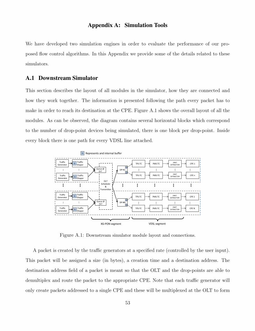
Appendix A: Simulation Tools
We have developed two simulation engines in order to evaluate the performance of our pro-
posed flow control algorithms. In this Appendix we provide some of the details related to these
simulators.
A.1 Downstream Simulator
This section describes the layout of all modules in the simulator, how they are connected and
how they work together. The information is presented following the path every packet has to
make in order to reach its destination at the CPE. Figure A.1 shows the overall layout of all the
modules. As can be observed, the diagram contains several horizontal blocks which correspond
to the number of drop-point devices being simulated, there is one block per drop-point. Inside
every block there is one path for every VDSL line attached.
VDSL segment
Traffic Generator
Traffic Shaper
Traffic Generator
Traffic Shaper
…
…
…
Traffic Generator
Traffic Shaper
Queue @ OLT
Traffic Generator
Traffic Shaper
…
…
DP #1
DP #N
OLT Scheduler
& Transmitter
…
Q
Q
…
Q
Q
…
Q
Q
Q
Q
Queue @ OLT
CPE 1
CPE n
…
PMS-TC
PMS-TC
…
TPS-TC
TPS-TC
…
ENET EXTRACTOR
ENET EXTRACTOR
…
…
CPE 1
CPE N
…
PMS-TC
PMS-TC
…
TPS-TC
TPS-TC
…
ENET EXTRACTOR
ENET EXTRACTOR
…
…
…
…
…
XG-PON segment
Q Represents and internal buffer
Figure A.1: Downstream simulator module layout and connections.
A packet is created by the traffic generators at a specified rate (controlled by the user input).
This packet will be assigned a size (in bytes), a creation time and a destination address. The
destination address field of a packet is meant so that the OLT and the drop-points are able to
demultiplex and route the packet to the appropriate CPE. Note that each traffic generator will
only create packets addressed to a single CPE and these will be multiplexed at the OLT to form
53

a PHY frame. The newly generated packets are transmitted to a dedicated the traffic shaper as
shown in Figure A.1. At the traffic shaper, the arriving packet is placed in an internal queue,
and a packet arrival event will be triggered. The traffic shaper will then compare the size of the
head-of-the-line (HOL) packet to the number of available credits. The HOL packet will not be
forwarded to the OLT until enough credits have been generated. The pseudocode logic for the
traffic shaper is shown in Figure A.2.
Figure A.2: Traffic Shaper Pseudo Code
The OLT queue contains all the incoming traffic from a specific drop-point device i.e. it
contains the traffic from all VDSL lines attached to that drop-point. In a system with 4 drop-
points and 2 VDSL lines per drop-point, there will be 4 queues at the OLT each containing the
traffic of their respective DSL line. The OLT will dequeue packets in a round-robin fashion and
insert them into the payload of a XG-PON PHY frame. The OLT will keep dequeueing packets
until the available payload in the current PHY frame is not enough or all queues become empty,
whichever occurs first. Once all packets available for transmission have been dequeued, the OLT
will then pause 125 µsec. This delay corresponds to the transmission time of a downstream
PHY frame in the XG-PON protocol. This is an important assumption made in the simulator:
a PHY packet is fully assembled before it is transmitted to the drop-points. After
the delay period, the OLT will send a START OF FRAME signal to all drop-points and then
54

forward the packets to the destination drop-point.
Once a drop-point starts receiving frames via its PON input port, it will look for a START-OF-
FRAME packet (which will precede all other packets in the frame) and pause for its corresponding
propagation delay. After this delay, the drop-point will receive the transmitted packets, check
their destination address field and place them in their corresponding VDSL output queue. The
drop-point will continue this process until another START-OF-FRAME packet is received and
the cycle restarts. Another important assumption in the model is that a drop-point will only
forward the encapsulated packets once it has received the complete PHY frame from
the OLT. This is mainly done in order to simply the computational expenses of transmitting
one packet at a time.
The packets at the drop-point are then queued in a per DSL buffer. The VDSL lines will
then extract packets from their corresponding buffer and encapsulate them into one or more
codewords as it would normally be done by the TPS-TC process. These codewords are then be
sent to the PMS process which further encapsulates them into DTU frames. Once a DTU frame
has been assembled with A codewords, it will be transmitted through the DSL line and reach an
Ethernet extractor process. This process will remove the DTU and codeword encapsulation and
transmit the packet to the receiving CPE. At the CPE, the packet statistics get recorded and it
is then removed from the system.
A.2 Upstream Simulator
The upstream simulator is a more complex simulation engine and only the main characteristics
related to this study will be described. Figure A.3 shows the overall layout of the simulator.
Packets are generated at the traffic generator modules which can be configured to produce
traffic with distinct distribution and variable bitrates. The generated packets travel through
the VDSL modules the same as how they traveled in our downstream simulator. Once packets
reach the drop-point, they will sit in a per DSL dedicated queue until they are scheduled for
”depature” by the OLT scheduling engine. A list of supported simulator features relevant to our
55
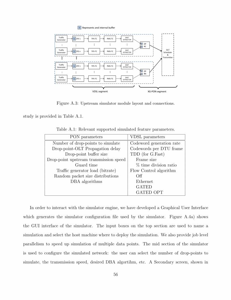
XG-PON segment VDSL segment
…
Traffic Generator
…
DP #N
OLT Scheduler
& Transmitter
CPE n
…
PMS-TC
PMS-TC
…
TPS-TC
TPS-TC
…
ENET EXTRACTOR
ENET EXTRACTOR
…
…
…
… …
Q Represents and internal buffer
Traffic Generator
CPE 1 Q
Q
Q
Traffic Generator
…
DP #1
CPE n
…
PMS-TC
PMS-TC
…
TPS-TC
TPS-TC
…
ENET EXTRACTOR
ENET EXTRACTOR
…
Traffic Generator
CPE 1 Q
Q
Q
Q
Q
Figure A.3: Upstream simulator module layout and connections.
study is provided in Table A.1.
Table A.1: Relevant supported simulated feature parameters.
PON parameters VDSL parameters
Number of drop-points to simulate Codeword generation rateDrop-point-OLT Propagation delay Codewords per DTU frame
Drop-point buffer size TDD (for G.Fast)Drop-point upstream transmission speed Frame size
Guard time % time division ratioTraffic generator load (bitrate) Flow Control algorithm
Random packet size distributions OffDBA algorithms Ethernet
GATEDGATED OPT
In order to interact with the simulator engine, we have developed a Graphical User Interface
which generates the simulator configuration file used by the simulator. Figure A.4a) shows
the GUI interface of the simulator. The input boxes on the top section are used to name a
simulation and select the host machine where to deploy the simulation. We also provide job level
parallelism to speed up simulation of multiple data points. The mid section of the simulator
is used to configure the simulated network: the user can select the number of drop-points to
simulate, the transmission speed, desired DBA algortihm, etc. A Secondary screen, shown in
56

Figure A.4b) contain the available VDSL configuration parameters.
a) Main screen b) VDSL configuration parameters
Figure A.4: Upstream simulator GUI interface.
We have also added some feature to help with the data visualization once a simulation finishes
execution. Some of these feature include: data retrieval and automatic graph generation.
57
Curriculum Vitae
Elliott Ivan Gurrola was born in Durango, Dgo. Mexico. In 2008 he joined the University of
Texas at El Paso (UTEP) to pursue a Bachelors of Science in Electrical Engineering. Upon
admission, Elliott was awarded the Presidential Excellence Scholarship. During his second year,
Elliott was selected for a teacher’s assistant position in the Physics Department for the Intro-
ductory Mechanics and the Fields and Waves courses; Elliott held this position for three years
and won the outstanding teacher assistant award in spring 2010. In summer 2011 Elliott was
accepted to participate at Purdue’s University Summer Fellowship program, where he joined the
Network for Photovoltaic Technology to develop a solar panel simulator. Elliott also worked as
an undergraduate research assistant for the Mechanical Engineering department developing and
designing autonomous navigation and control systems.
Elliott graduated Summa cum Laude in Fall 2011. After graduation, he was accepted into
the Computer Engineering Masters program at UTEP. As a graduate student, Elliott joined
the Networks and Communications Lab under the supervision of Dr. Michael McGarry. As
a graduate researcher, he helped develop simulation experiments for passive optical networks.
Elliott also developed a series of automation scripts used for processing data and simulation
monitoring. He contributed to the publication of On the Reduction of ONU Upstream Buffering
for PON/xDSL Hybrid Access Networks and Downstream ONU Buffer Modeling for Fiber to the
Drop-point, which he co-authored.
Permament Address: Elliott I. Gurrola
640 Bristol Dr.
El Paso, TX. 79912
USA
58