Reducing the Tuning Effort of a Steer-Torque-Manager for Vehicle Lateral Control

OLA WALLNÄS

Master of Science Thesis

Stockholm, Sweden 2015

Reducing the Tuning Effort of a Steer-Torque-Manager for Vehicle Lateral Control

Ola Wallnäs

Master of Science Thesis MMK 2015:29 MDA 505

KTH Industrial Engineering and Management

Machine Design

SE-100 44 STOCKHOLM

Master of Science Thesis MMK 2015:29 MDA 505

Reducing the Tuning Effort of a Steer-Torque-Manager for Vehicle Lateral

Control

Ola Wallnäs

Approved

2015-06-05

Examiner

Lei Feng

Supervisor

Daniel Frede

Company partner

Volvo Cars

Company contact person

Martin Distner

Abstract

A lot of research and development in the automotive industry today is focusing on active safety

and driver assistance functions. On the market there are already car models with the ability to

provide autonomous steering and behind next door stands the fully autonomous vehicles.

The steering functionality is often referred to as Lane Keeping or lateral control. When its

operation is verified in one vehicle it needs to be introduced into the following vehicles models

as efficiently as possible. Aspects like vehicle dynamics together with system and component

responses require the need for tuning and modification for each new vehicle model. One

software component in the steering functionality that needs extensive tuning is the module

determining the steer torque request that is sent to the Electric Power Steering (EPS). This

component is referred to as the Steer-Torque-Manager (STM).

In this thesis an investigation takes place regarding how the tuning effort of the STM can be

reduced with help from model-based development and what the requirements for this are. To

achieve this two virtual vehicle models including a steering system model are evaluated against

physical measurements from a Volvo XC90. The first one is a model created in the software

CarMaker and Simulink and the second one is a co-simulation model between Adams and

Simulink. To evaluate the significance of certain parameters and settings a sensitivity analysis is

performed. With the objective to evaluate if the existent STM controller can be modified to

allow more rapid tuning a Two-Degree-Of-Freedom (2-DOF) controller, an Internal Model

Control (IMC) controller and a Self-Tuning Regulator (STR) are implemented and evaluated.

The results show that the accuracy of the co-simulation model is sufficient to make it useful in

the design and tuning of the STM and that the characteristics of the torsion bar, steering column

and steering wheel has a large impact on the system response. From the control investigation it

can be concluded that the 2-DOF controller has the ability to simplify the tuning and slightly

improve the performance, while the IMC controller decreases the performance and the STR

suffers from implementation issues.

Examensarbete MMK 2015:29 MDA 505

Reducering av inställningsbehovet av en

Steer-Torque-Manager för lateral fordonsreglering

Ola Wallnäs

Godkänt

2015-06-05

Examinator

Lei Feng

Handledare

Daniel Frede

Uppdragsgivare

Volvo Cars

Företagskontakt

Martin Distner

Sammanfattning

Mycket forskning och utveckling inom fordonsindustrin i dag fokuserar på aktiv säkerhet och

förarassistansfunktioner. På marknaden finns redan bilmodeller som har möjlighet att erbjuda

autonom styrning och bakom nästa hörn står helt autonoma fordon.

Styrfunktionaliteten refereras ofta till genom termen Lane Keeping och när dess funktion är

verifierad för ett fordon måste den införas i efterföljande fordon så effektivt som möjligt.

Aspekter såsom fordonsdynamik samt system- och komponentsvar skapar ett behov av

inställning och anpassning för varje ny bilmodell. En mjukvarukomponent som i synnerhet är i

behov av anpassning är funktionen som fastställer styrmomentbegäran som skickas till den

elektriska styrservon (EPS). Denna komponent kallas för Steer-Torque-Manager (STM).

I denna avhandling genomförs en undersökning om hur anpassningsbehovet av STM kan

minskas med hjälp av modellbaserad utveckling och vilka kraven för detta är. För att uppnå detta

utvärderas två virtuella bilmodeller, innehållande en modell över bilens styrsystem mot fysiska

mätningar ifrån en Volvo XC90. Den första modellen är skapad i mjukvaran CarMaker och

Simulink och den andra är en co-simulering mellan Adams och Simulink. För att utvärdera

betydelsen av vissa parametrar och inställningar så genomförs en känslighetsanalys. I syfte att

undersöka om den existerande STM regulatorn kan modifieras för att möjliggöra snabbare

inställning, så har också en 2-DOF regulator, en IMC regulator och en självinställande regulator

(STR) skapats och testats.

Resultaten visar att noggrannheten hos co-simuleringsmodellen är tillräcklig för att göra den

användbar i designen och inställningen av STM och att egenskaperna hos torsionsstaven,

rattstången och ratten har en stor inverkan på systemdynamiken. Reglerundersökningen pekar på

att 2-DOF regulatorn kan möjliggöra snabbare inställning och något förbättrad prestanda, medan

IMC regulatorn försämrar prestandan och att STR lider av implementationssvårigheter.

FOREWORD

First of all, I would like to send my gratitude to all the people around me at Active Safety and

CAE Vehicle Dynamics departments at Volvo Car Corporation that have provided support and

given me an enjoyable and motivating environment to spend my days in. Special thanks go to

Lars Johannesson Mårdh for your valuable inputs regarding control theory, Andreas Johansson

for STM support, my industrial supervisors Daniel Gunnarsson and Markus Löfgren, Fredrik

Warnström for Adams support and of course Marcus Ljungberg for all your help regarding both

the CarMaker and the co-simulation model. Furthermore I also want to express my gratitude

towards my university supervisor in Stockholm Daniel Frede, my examiner Lei Feng and my

coordinator Fredrik Asplund, who have taken care of administrative issues, improved the

scientific methodology and given me continuous feedback of my progress. Since this document

will also be my last deliverable as a graduate, I finally want to thank you, my beloved Åsa, for

all your support and love throughout my studies.

Ola Wallnäs

Gothenburg, June, 2015

ABBREVIATIONS

AWD All Wheel Drive

CAD Computer Aided Design

CAN Controller Area Network

CAE Computer Aided Engineering

c.g. Centre of Gravity

DOF Degrees Of Freedom

ECU Electronic Control Unit

EPS Electric Power Steering

FOPDT First-Order Plus Dead Time

IMC Internal Model Control

KTH Kungliga Tekniska Högskolan/ Royal Institute of Technology

LKA Lane Keeping Aid

MIMO Multiple Input Multiple Output

PID Proportional, Integral and Derivative

SISO Single Input Single Output

STM Steer Torque Manager

STR Self-Tuning Regulator

TABLE OF CONTENTS

1 INTRODUCTION ................................................................................................................................................... 1

1.1 SYSTEM OVERVIEW AND BACKGROUND ........................................................................................................................ 1 1.2 PURPOSE ............................................................................................................................................................... 4 1.3 DELIMITATIONS ....................................................................................................................................................... 4 1.4 METHOD ............................................................................................................................................................... 5 1.5 SOCIAL AND ETHICAL ASPECTS .................................................................................................................................... 5

2 FRAME OF REFERENCE ........................................................................................................................................ 7

2.1 SYSTEM IDENTIFICATION THEORY ................................................................................................................................ 7 2.2 STEERING SYSTEM MODELLING ................................................................................................................................... 8 2.3 RELATED CONTROL THEORY ..................................................................................................................................... 12

3 PHYSICAL MEASUREMENTS ............................................................................................................................... 19

4 MODELLING ...................................................................................................................................................... 21

4.1 DESCRIPTION OF MODELS ........................................................................................................................................ 21 4.2 MODEL EVALUATIONS ............................................................................................................................................ 26

5 CONTROL .......................................................................................................................................................... 37

5.1 CONTROL IMPLEMENTATIONS .................................................................................................................................. 37 5.2 CONTROL EVALUATIONS .......................................................................................................................................... 43

6 DISCUSSION AND CONCLUSIONS ....................................................................................................................... 47

6.1 DISCUSSION ......................................................................................................................................................... 47 6.2 CONCLUSIONS ...................................................................................................................................................... 48

7 RECOMMENDATIONS AND FUTURE WORK ....................................................................................................... 51

7.1 RECOMMENDATIONS ............................................................................................................................................. 51 7.2 FUTURE WORK ...................................................................................................................................................... 51

8 REFERENCES ...................................................................................................................................................... 53

APPENDIX A: SELECTION OF INTERVIEW QUESTIONS

APPENDIX B: TIRE COMPARISON

APPENDIX C: SENSITIVITY ANALYSIS RESULTS

1

1 INTRODUCTION

This chapter serves to introduce the system and to state the background, the purpose, the

delimitations and the method used.

1.1 System overview and background

Within this section an overview of the system/plant is provided, which has been created from

material at Volvo Cars and from interviews. A selection of the interview questions can be found

in Appendix A.

1.1.1 The steering system

There exists a wide range of different steering configurations, covered in literature as [1] and [2].

The steering system described in this report belongs to the Volvo XC90 (2015) and is

manufactured by a sub-supplier. A schematic picture of it can be seen in Figure 1, and it can be

described as an electro-mechanical rack and pinion system.

Figure 1. Graphical representation of the steering system in use (not the actual one) [3].

The tie rods have side take-off, the pinion gear is situated on the left hand-side and the electrical

motor acts on the rack through a belt-driven ball screw. A collapsible steering column with two

universal joints is used to transfer the torque from the driver. To measure the torque resulting

from rack forces and from driver manoeuvres, a torsion bar is also situated in the connection

between the pinion and the steering column. When it comes to the steering geometry, the

Ackermann principle is used. The adopted steering linkage configuration or suspension design is

double wishbone.

Earlier, different types of hydraulic power steering systems were commonly used in order to

reduce the driver torque required to turn the wheels and thereby to improve the handling of the

vehicle. In these systems the oil provided some damping and the magnitude of the applied

2

additional force was often dependent on the current vehicle speed [2]. Also in recently developed

electric power steering (EPS) systems, like the one in Figure 1, these functionalities and even

more are provided and realized by software functions embedded in the software controlling the

electric motor. For this reason the “steering feel” and steering response is greatly affected by the

structure of the software. One example is that the speed dependency of the assistance force is

implemented using the measure torsion bar torque and Boost-curves in the software.

1.1.2 Autonomous steering

Today active safety functions that provide automatic steering for cars are getting more common.

This steering functionality provides lateral control of the vehicle and is often referred to as LKA

(Lane Keeping Aid) for example, which is a customer function name used by Volvo Cars. The

system covered in this report receives information about the lane markings and the surroundings

from a module consisting of a radar and a camera mounted in the upper part of the windshield.

An Electronic Control Unit (ECU) analyses the information. If any of the autonomous steering

functions are active, a desired pinion angle request is calculated based on a heading offset

between the actual and the desired path of the vehicle. This pinion angle is then sent to the Steer-

Torque-Manager (STM). The mission of this software function is to determine the right amount

of equivalent torque to be applied on the rack by the electronic motor in order to obtain a certain

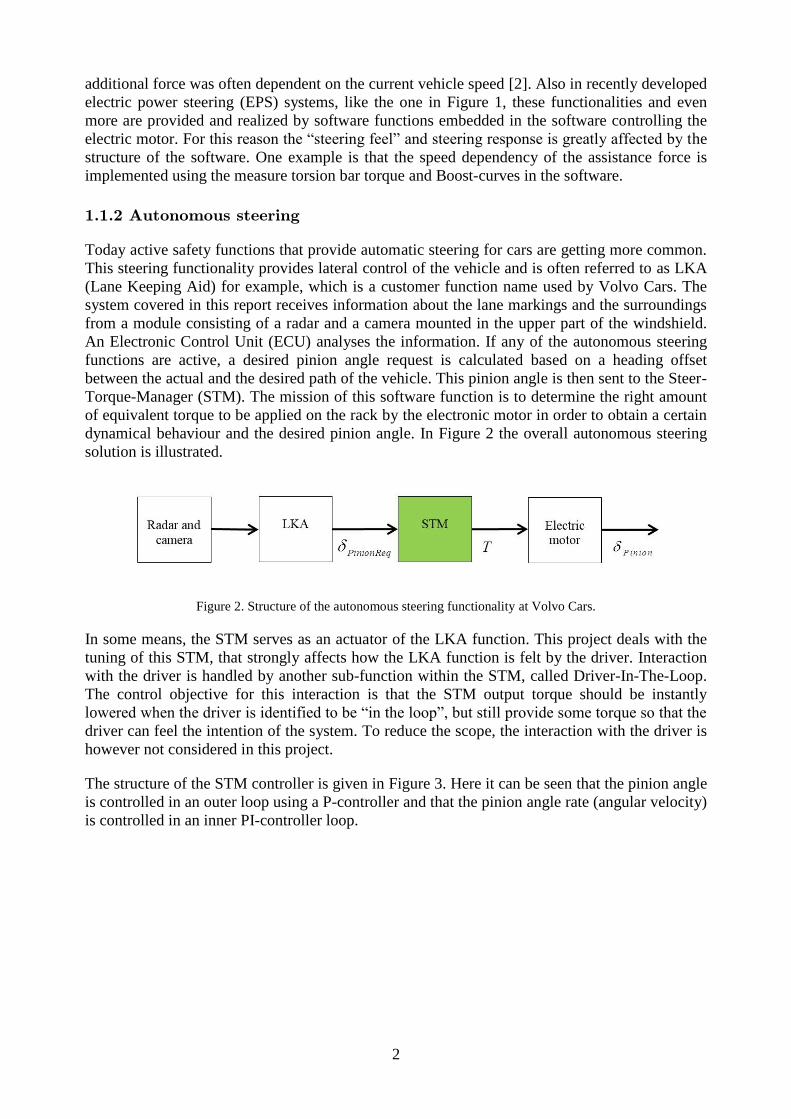
dynamical behaviour and the desired pinion angle. In Figure 2 the overall autonomous steering

solution is illustrated.

Figure 2. Structure of the autonomous steering functionality at Volvo Cars.

In some means, the STM serves as an actuator of the LKA function. This project deals with the

tuning of this STM, that strongly affects how the LKA function is felt by the driver. Interaction

with the driver is handled by another sub-function within the STM, called Driver-In-The-Loop.

The control objective for this interaction is that the STM output torque should be instantly

lowered when the driver is identified to be “in the loop”, but still provide some torque so that the

driver can feel the intention of the system. To reduce the scope, the interaction with the driver is

however not considered in this project.

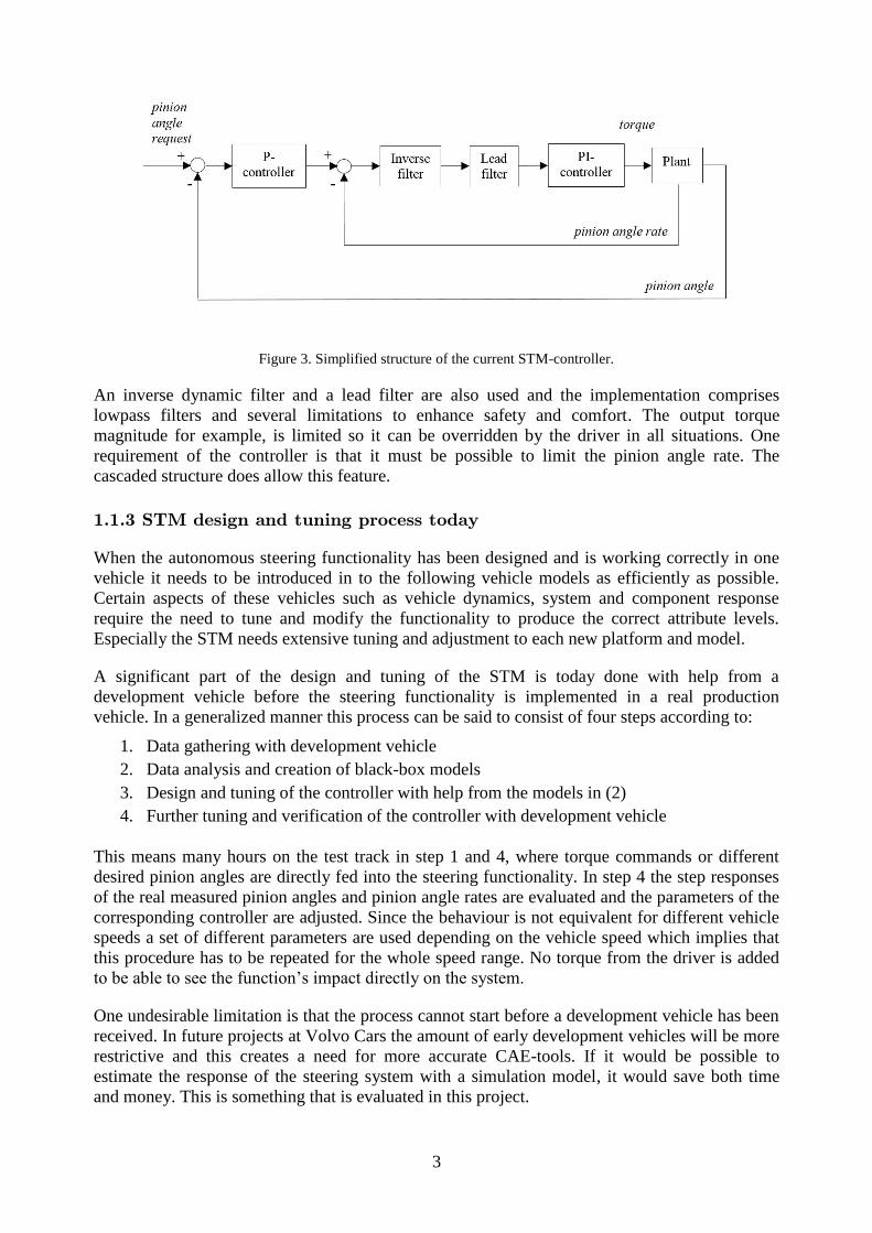
The structure of the STM controller is given in Figure 3. Here it can be seen that the pinion angle

is controlled in an outer loop using a P-controller and that the pinion angle rate (angular velocity)

is controlled in an inner PI-controller loop.

3

Figure 3. Simplified structure of the current STM-controller.

An inverse dynamic filter and a lead filter are also used and the implementation comprises

lowpass filters and several limitations to enhance safety and comfort. The output torque

magnitude for example, is limited so it can be overridden by the driver in all situations. One

requirement of the controller is that it must be possible to limit the pinion angle rate. The

cascaded structure does allow this feature.

1.1.3 STM design and tuning process today

When the autonomous steering functionality has been designed and is working correctly in one

vehicle it needs to be introduced in to the following vehicle models as efficiently as possible.

Certain aspects of these vehicles such as vehicle dynamics, system and component response

require the need to tune and modify the functionality to produce the correct attribute levels.

Especially the STM needs extensive tuning and adjustment to each new platform and model.

A significant part of the design and tuning of the STM is today done with help from a

development vehicle before the steering functionality is implemented in a real production

vehicle. In a generalized manner this process can be said to consist of four steps according to:

1. Data gathering with development vehicle

2. Data analysis and creation of black-box models

3. Design and tuning of the controller with help from the models in (2)

4. Further tuning and verification of the controller with development vehicle

This means many hours on the test track in step 1 and 4, where torque commands or different

desired pinion angles are directly fed into the steering functionality. In step 4 the step responses

of the real measured pinion angles and pinion angle rates are evaluated and the parameters of the

corresponding controller are adjusted. Since the behaviour is not equivalent for different vehicle

speeds a set of different parameters are used depending on the vehicle speed which implies that

this procedure has to be repeated for the whole speed range. No torque from the driver is added

to be able to see the function’s impact directly on the system.

One undesirable limitation is that the process cannot start before a development vehicle has been

received. In future projects at Volvo Cars the amount of early development vehicles will be more

restrictive and this creates a need for more accurate CAE-tools. If it would be possible to

estimate the response of the steering system with a simulation model, it would save both time

and money. This is something that is evaluated in this project.

4

The existing STM controller delivers satisfying results, but due to time limitations it has not been

evaluated against any other possible control structures. Both the inverse- and the lead filter have

been added in an ad hoc manner, instead of integrated together with the PI-controller. One part

that has been especially time consuming to derive is the system inverse, which is a 6th order

polynomial. The design of the PI-controller was handled by manually tuning its parameters to get

a good response and the lead filter was added to get a phase lift in a certain region. In other

words the design of the inner loop has been done by shaping the time and frequency responses.

One goal of this thesis is to evaluate the design of the inner loop and investigate if it can be

restructured in order to make the tuning easier and faster.

The outer loop that comprises a P-controller, is adaptive with regard to the vehicle speed as one

of the parameters. This means that different gains are used in different regions, which is known

as gain scheduling, where the different gains are optimized according to several cost functions

and determined by usage of the software ModeFrontier. To make the scope manageable and due

to license restrictions, the design and tuning of the outer loop is not investigated any further in

this project.

1.2 Purpose

The main goal of the thesis is to investigate how the effort for tuning of the Steer-Torque-

Manager (STM) can be reduced by addressing the problem through CAE and model-based

development. Specifically, the project aims to investigate the requirements for implementing

model-based tuning in this context and to enlarge the knowledge about which parameters affect

system behaviour. One subtask is also to benchmark the existing pinion angle rate controller. To

achieve the stated goals, two research questions have been formulated as follows:

Which requirements exist for a vehicle model in order to make the design and tuning of a

“Steer-Torque-Manager” more efficient?

Can the currently used controller (cascaded PI-controller with inverse filtering and

phase compensation) be modified or exchanged to a controller allowing more rapid

tuning without losing performance*?

1.3 Delimitations

The main delimitations of the project have already been mentioned and in this section the

complete set is summarized:

The steering wheel torque provided by the driver is assumed to be strictly zero

throughout the whole project

Regarding the STM-controller, the design and tuning of the outer cascade loop is not

investigated

Only normal, dry road conditions have been considered

All modelling and verification activity is limited to one vehicle model

*Not losing performance is here defined as having no static error and an equivalent (± 10 %) rise time and overshoot

with the existing controller.

5

1.4 Method

To ensure that the goals of the project will be fulfilled, the two above research questions have

been formulated to provide guidance in the investigation. Answering the research questions

using appropriate methods has been the main focus. One question, as well as one part of the

report, is focusing on modelling and the other one is focusing on control.

The first research question has mainly been investigated by evaluating the accuracy of two

different vehicle models, comprising the steering system, against real car measurements. By

performing a sensitivity analysis on the most accurate model, the significance of different

parameters and settings has also been evaluated. Throughout the project, collection of existing

knowledge at the company has been essential. For this purpose semi-structured interviews were

done with a few carefully chosen persons. Information has been gathered using unstructured

interviews also, but semi-structured interviews were deemed most appropriate in order to both

receive a large amount of qualitative data and to get direct answers to specific questions. A

selection of the interview questions can be found in Appendix A, and the answers received have

been summed up and expressed in other words because no audio recording took place (see

Section 1.5). The interview questions have not been used in any announced interview sessions,

but within the frame of an ordinary meeting, or one-at-a-time directly at the working desk when

time has allowed it. This adaptation was deemed suitable to use at Volvo Cars.

The second question has partly been answered through a literature study covering state-of-the-art

control solutions and with help from this material, three alternative control structures have been

proposed and compared with the original structure using simulations on the most accurate

vehicle model.

1.5 Social and ethical aspects

The intent of this thesis is to follow the directions and ethical policy from KTH. This includes

announcements of all scientific contributions to the thesis and to provide “adequate and fair

references”. When it comes to the people interviewed they were not formally told that they did

participate in an interview, which may be questionable. The participants’ name and exact

answers have however not been documented and the interviews have not been recorded, which

justifies this choice.

A well formulated model-based design and tuning process increases the chances of a more

reliable lateral control function and reduces the amount of early physical testing. This can

improve the working environment for the development engineers since the physical tuning

involves turning in high speeds without any steering wheel contact. Also in an economical and

an environmental aspect a more sustainable development can be achieved with less physical

testing. Since the lateral steering functionality is a safety critical function, its design and

robustness are critical. Safety aspects and existing safety framework surrounding the

functionality are not covered in this thesis and the function will always need to be verified using

a real vehicle, no matter how good the virtual tuning may be.

6

7

2 FRAME OF REFERENCE

In this chapter the main part of knowledge gained from the relating literature can be reviewed.

2.1 System identification theory

When it comes to identification of a dynamical system the perhaps most intuitive approach is to

model the system behaviour with help from applicable physical laws. In the scope of this project,

more than one comprehensive physical model was identified to exist within the company during

the pre-study phase. For controller purposes a simplified, linear model however is desirable and

in order to gain knowledge of the system some appropriate methods have to be used. For these

reasons a short literature review of existing system identification methods are presented in this

section.

2.1.1 Nonparametric identification

There are several ways of identifying a system and creating a model of it. Firstly, there are

nonparametric identification methods. In the time domain this can be done using transient

analysis if it is possible to perform step inputs to the system. If the input signal u(t) instead is just

measurable but not controllable, a correlation analysis between the chosen in- and output signal

y(t) can be done. This assumes that the two signals are uncorrelated and can be performed by

first removing the means and filter both signals through the same filter to approximate them as

white noise. The estimation of the transient behaviour is then given with help from the variance

of u(t) and the covariance. As for transient analysis, correlation analysis can be very useful in an

initial phase to give information about time delays, time constants, signal relationships and static

signal levels, but it does not directly produce a model of the system.

It is also common to perform a nonparametric identification in the frequency domain, which can

deliver an approximation of the bode diagrams and the transfer function G(iw) between the

measured signals. This approach is especially suited to find or to investigate frequencies of

particular interest if the system can be seen as linear. One way is to use input on the form

u(t)=u0cos(wt) and repeat the procedure for all relevant frequencies w. If this is not possible

spectral analysis can be used instead if the two signals are uncorrelated. The implementation of

such an analysis usually includes removal of means, the usage of a window function and

variance functions for u(t) and y(t) to derive estimations of the spectral densities. One example of

a window function that can be used to reduce the fluctuations originating from disturbances is

the Hann filter. The transfer function between u(t) and y(t) can be approximated from the

spectral densities and the spectral density for the disturbances [4].

2.1.2 Parametric identification

When it comes to parametric identification methods one common division is to distinguish

between models derived from physical laws (white box models) and models derived from in- and

output signals with no or limited knowledge about the physical system (black box models).

Usage of white box models will obviously generate more insight of the system. If some

parameter values are missing these may have to be identified through experiments. A black box

model can be used if the physical relationships of the system are too hard to estimate, if the time

is limited, if a linear model is required, or if the only aim with the model is to predict future

output values. This method includes gathering a set of in- and output data, deciding upon a

suitable model structure to use and finding the set of model parameters that minimizes the

prediction error. A great deal of work in this process is the choice of model structure, which first

8

involves choosing a suitable polynomial model structure and then suitable values on the design

parameters determining the number of poles and zeroes and the delay. It is important that the

input signal excite all frequencies and magnitudes of relevance and for this white noise is

preferable, which may not be possible to use on the physical system.

Sometimes the system is too nonlinear or the intended use of the model requires usage of a

nonlinear model. In this case a multiple of different parameter sets together with a linear model

can be used and combined differently in different regions. Local models based on a weighted

mean value of previous measured data are another option which requires knowledge of the noise

levels and smoothness of the function itself. Usage of nonlinear parametric models can also be

done, where Artificial Neural Networks are possible to use in the multidimensional case. This

means basically using a combination of one nonlinear base function with different gains/weights

in a significant number of different subspaces of a multidimensional solution space [4], [5]. A

large set of in- and output measurements are then required to “teach” the network; i.e. to

determine the weights [6].

2.1.3 Least squares

One very common specific method that is used for parametric identification in the time domain

is least squares. This method usually forms the basis when determining the parameters of

different model structures. The least squares is built upon minimizing the squared sum of

differences between estimated output and measured output and for a linear discrete model

expressed as

1 1 2 2

1 2

1 2

ˆ( ) ( ) ( ) ... ( ) ( )

( ) ( ( ) ( ) ... ( ))

( ... )

T

n n

T

n

T

n

y i i i i i

i i i i

(1)

, the least squares is the solution of the parameter vector that minimizes the function

2

1

1( , ) ( ( ) ( ) )

2

tT

i

V t y i i

(2)

The vector is called the regression vector and contains known functions that are together with

the measured system outputs ( ( ), ( )),i 1,2,..., ty i i , obtained from experiments [7]. In addition

to this standard expression, there also exists several variants and extensions of the least square

algorithm, where least mean squares, projection algorithm, stochastic approximation and

recursive least square are some to be mentioned. In Wittenmark et al. [7] these variants where

compared through simulations and the recursive least square showed a superior convergence

behaviour, but with a higher computational cost.

2.2 Steering system modelling

This section presents an overview of steering system modelling found in literature mostly

dealing with lane keeping control applications. The details are not covered, but can be found in

the references.

In order to be able to simulate the behaviour of a steering system during steering manoeuvres a

model of the complete vehicle is needed. The dynamics of the complete vehicle will affect the

9

forces acting on the steering system through the tires and through the forces acting on the tie rods

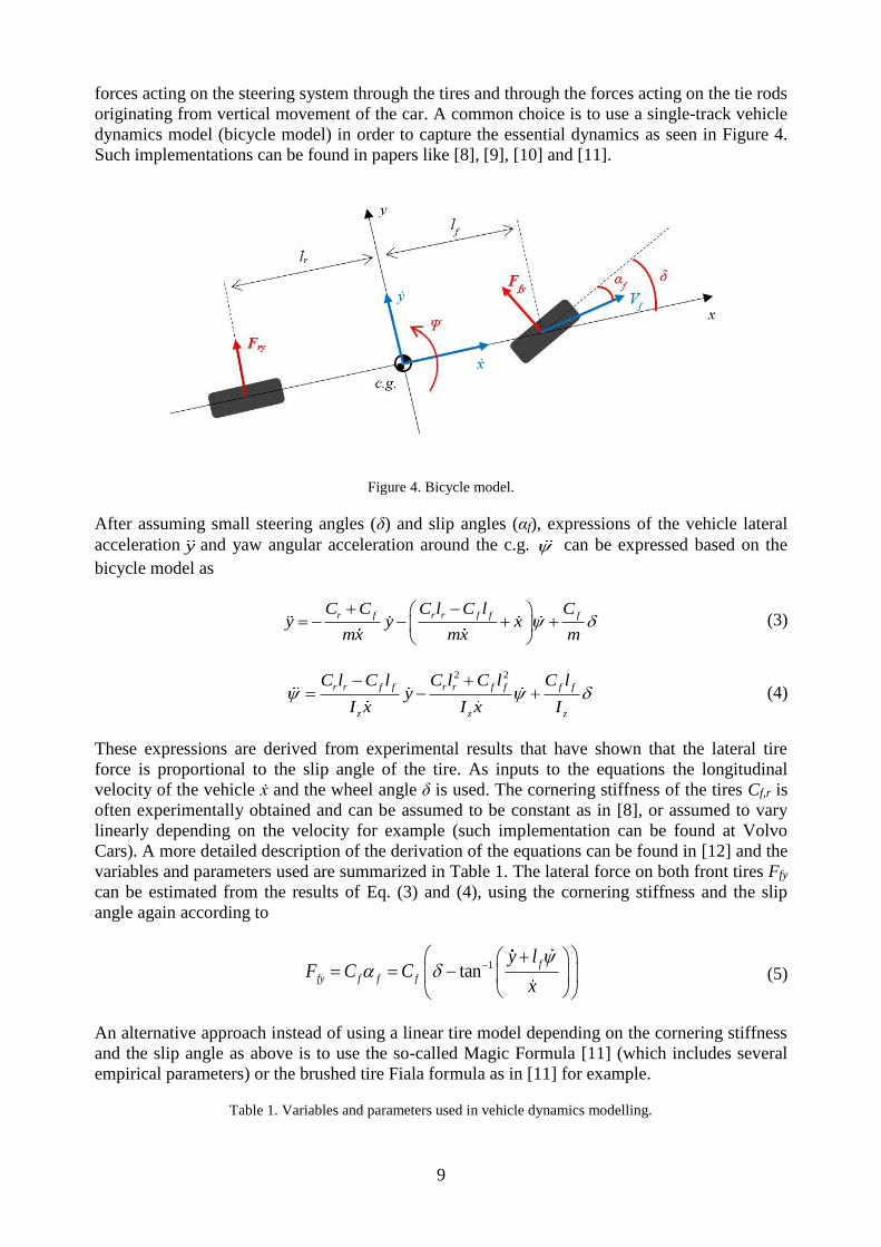
originating from vertical movement of the car. A common choice is to use a single-track vehicle

dynamics model (bicycle model) in order to capture the essential dynamics as seen in Figure 4.

Such implementations can be found in papers like [8], [9], [10] and [11].

Figure 4. Bicycle model.

After assuming small steering angles (δ) and slip angles (αf), expressions of the vehicle lateral

acceleration y and yaw angular acceleration around the c.g. can be expressed based on the

bicycle model as

r f r r f f fC C C l C l Cy y x

mx mx m

(3)

2 2

r r f f r r f f f f

z z z

C l C l C l C l C ly

I x I x I

(4)

These expressions are derived from experimental results that have shown that the lateral tire

force is proportional to the slip angle of the tire. As inputs to the equations the longitudinal

velocity of the vehicle ẋ and the wheel angle δ is used. The cornering stiffness of the tires Cf,r is

often experimentally obtained and can be assumed to be constant as in [8], or assumed to vary

linearly depending on the velocity for example (such implementation can be found at Volvo

Cars). A more detailed description of the derivation of the equations can be found in [12] and the

variables and parameters used are summarized in Table 1. The lateral force on both front tires Ffy

can be estimated from the results of Eq. (3) and (4), using the cornering stiffness and the slip

angle again according to

1tan

f

fy f f f

y lF C C

x

(5)

An alternative approach instead of using a linear tire model depending on the cornering stiffness

and the slip angle as above is to use the so-called Magic Formula [11] (which includes several

empirical parameters) or the brushed tire Fiala formula as in [11] for example.

Table 1. Variables and parameters used in vehicle dynamics modelling.

10

Symbol Description Unit

m

Iz

g

lf, lr

δ

αf

Ψ

ẋ, ẏ

Vf

Cf, Cr

Ffy, Fry

Vehicle mass

Moment of inertia around the z axis at the c.g.

Gravity acceleration constant

Distance from c.g. to rear and front axles

Average wheel steering angle

Slip angle of the front tires

Yaw of the vehicle around c.g.

Vehicle velocity at the c.g. in the x- and y direction

Velocity vector at the front axle

Cornering stiffness of front and rear tires

Lateral forces acting on front and rear tires

kg

kgm2

m/s2

m

rad

rad

rad

m/s

m/s

kN/rad

N

When it comes to modelling the steering system, it is common to assume the column as one stiff

bar together with a fixed gear ratio for the rack and pinion. The steering linkage geometry is

often not covered in detail, unless it is generated from a CAD software or equivalent. In Figure 5

a simplified model of the steering system is shown.

Figure 5. Steering system model.

The force acting on the rack through the tie rods Frod are derived from a self-aligning moment

Talign and a moment Tlift resulting from the vertical movement of the car described in [13]. In [14]

a friction torque from the road-tire interface is also included. The self-aligning moment

described in [15] results from the lateral wheel force and its moment arm created by the

pneumatic trail Lpt (the tire deformations are asymmetric) and the caster/mechanical trail Lmt (due

to kingpin geometry). Following the same methodology as presented in [8], the equations for the

system can be expressed as

s sw d tJ T T (6)

r rt t sw s sw

e e

x xT k b

r r

(7)

tr r EPS r r rod

e

Tm x F b x F

r (8)

11

( )EPS EPS EPS boost d STMF n k P T T (9)

r armx L (10)

align lift

rod

arm

T TF

L

(11)

( )align fy pt mtT F L L (12)

( cos( )sin( )) sin( )lift dist c king fz kingT L F (13)

rfz

f r

mglF

l l

(14)

In the representation of the force FEPS provided by the EPS it is of course also possible to take

the motor characteristics into account and if a belt driven ball nut gear is used, it can be

appropriate to introduce some additional friction, an efficiency constant and a stiffness for

example. The scaling factor kEPS, represents the effect of all the unknown built-in software

functions in the EPS, in addition to the boost curve polynomial Pboost. This scaling factor may

also have a significant impact on a torque request TSTM that is fed directly into the EPS.

Definitions of variables and parameters are found in Table 2.

12

Table 2. Variables and parameters used in steering system modelling.

Symbol Description Unit

Js

mr

θsw

θc

θking

xr

Larm

Lpt

Lmt

Ldist

re

nEPS

kt

bs

br

kEPS

Pboost

Td

TSTM

Tt

Talign

Tlift

Frod

FEPS

Ffz

Inertia of steering column and steering wheel

Mass of rack, steering linkage and front wheels

Steering wheel angle

Caster angle

Kingpin inclination angle

Rack displacement

Length of link arm connecting the tie rod to the knuckle

Pneumatic trail (Offset for Ffy to the tire centre)

Mechanical trail (due to the θking)

Offset distance of the wheel centre to the steer axis

Pinion gear effective radius

Ball nut screw and belt drive effective gear ratio

Torsion bar stiffness

Steering column damping

Rack damping

Dynamical scale factor representing effect of EPS functions

Boost curve polynomial

Driver torque

Torsion bar torque

Steer-Torque-Manager torque request

Aligning moment on front wheels due to Ffy

Aligning moment due to vertical movements of the wheels

Forces acting on the rack through the tie rods

Electrical power steering force acting on the rack

Normal force at front axle

kgm2

kg

rad

rad

rad

m

m

m

m

m

m

m

Nm/rad

Nms/rad

Nms/rad

-

-

Nm

Nm

Nm

Nm

Nm

N

N

N

2.3 Related Control theory

This section has been created with both the objective to understand the current control

implementation and to investigate different applicable control structures. The study is focused on

methods/concepts already included in the current solution and on concepts that seemed

promising in the context of the thesis. Due to this reason nonlinear and MIMO control solutions

are not covered.

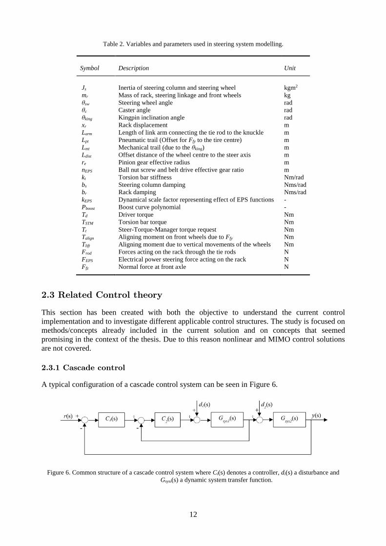
2.3.1 Cascade control

A typical configuration of a cascade control system can be seen in Figure 6.

Figure 6. Common structure of a cascade control system where Ci(s) denotes a controller, di(s) a disturbance and

Gsysi(s) a dynamic system transfer function.

13

As seen in this figure the system consists of two control loops, one outer and one faster inner

loop. This speed difference between the loops makes it possible to design the two control loops

separately. As an industry rule of thumb the inner loop should be at least five times faster to

make this possible [6]. The inner loop is designed first and then the outer one is designed by

treating the influence of the first loop as “1”. Cascaded control is particularly useful if a signal

“between” the in- and output signal of the whole control structure is measurable. Disturbances

acting on the inner loop can also be counteracted significantly faster. When controlling a position

or angle it is possible to exchange the derivative part of a single PID-controller against an inner

loop controlling the velocity. In this case the inner loop acts as a PD-controller without low-pass

filtering. The structure will however be more sensitive to non-modelled high frequency

dynamics, which motivates low-pass filtering of the velocity signal [16], [17]. One common

design choice is to use a P-controller for the inner loop. A PI-controller is needed if the inner

loop contains significant time delays and if the inner loop gain has to be limited. This will

however give the drawback of always creating an overshoot in the outer loop response [6].

According to Åström et al. [6] integral windup in the inner loop can be handled with

conventional methods, but if integral action is used also in the outer loop, it is not a trivial task to

avoid it.

2.3.2 Feedforward control

In most occasions when a disturbance is measurable the feedback controller can be successfully

extended with feedforward. By compensating for the known disturbance before the disturbance

has affected the system output makes this method effective in stabilizing the system [17]. When

it comes to usage of cascaded controllers, disturbances acting on the outer loop make it desirable

to include some setpoint tracking or servo functionality in especially the inner loop to enhance

the performance [18], which means using the system inverse 1 ( )sysG s

as a feedforward part. One

challenge in doing so is ensuring that the inverse of the system is implementable and stable. This

requires that the poles of 1 ( )sysG s

are situated on the left half-plane and that the order of its

denominator is at least as high as the order of its numerator. If this is not the case an

implementable approximation of the inverse has to be created. According to Lennartsson [17]

this can be done using a static approximation as 1 (0)sysG

or a dynamic approximation expressed as

* (s)( , , )

( ) ( ) ( , )m

AG s m

B s B s A s

(15)

, where

( ) (s) B ( )

( )( ) ( )

sys

B s B sG s

A s A s

(16)

and

1( , ) (1 )(1 )...(1 )m

mA s s s s (17)

Here B-(s) contains all unstable zeroes and B+(s) all stable ones. The constant α fulfils 0.5 ≤ α ≤ 1

and m shall be large enough to make sure that the order of the denominator is equal or of higher

order than the numerator in Eq. (15). If double poles are chosen (α=1), the constant τ can be

determined from a desired bandwidth wb according to

14

11

2 1m

bw (18)

The dynamic approximation requires that Gsys(s) is well known; otherwise the static

approximation is preferable. One example of how the inverse can be derived if the system model

is discrete is given in [19], where Okuyama et al. multiply the denominator of the inverse with

the discrete operator z to make it proper. The inverse model however has infinite gain at the

Nyquist frequency and therefore an additional filter is used to prevent vibrations.

2.3.3 Output error feedback (2-DOF control)

One way of increasing the flexibility of a conventional PID controller is to use output error

feedback or 2-DOF control. This means treating the reference input and the plant output

separately. By doing so, the controller’s capability of following the transient behaviour of the

reference signal and at the same time handle disturbances and noise increases. Regular feedback

acting on the error is forced to handle these two different control goals with the same set of

parameters. A general structure of the 2-DOF control is given in Figure 7, but of course several

different versions exist.

Figure 7. General structure of 2-DOF control.

One well-known structure is called setpoint weighting [3], [20], where the original PID

controller structure

1

( ) ( ( ) )dp d

i

deu t K e e s ds T

T dt (19)

is kept, but with the weights b and c in the error terms as p refe by y and d refe cy y . In this

setup the overshoot will decrease with a smaller value of b, and the parameter c is often chosen

to zero to avoid large transients if the setpoint includes step changes. If the controller is the

inner-loop of a cascaded structure however, the setpoint usually changes smoothly without any

steps [6]. The main disadvantage with setpoint weighting is that the responsiveness to setpoint

changes reduces when the overshoot is limited. In order to handle this some more complex

control schemes can be considered or inversion-based feedforward action, which is more

commonly used [20]. According to Wu et al. [21], design of such inversion-based 2-DOF is

almost exclusively performed in an ad hoc manner, by designing the feedback part first and then

the feedforward part separately. This may not lead to an optimal combination of the two

concepts. Therefore a concept based on a H∞ feedback controller which takes the feedforward

uncertainties into account is proposed [21]. This controller however does not have any focus on

efficient practical implementation and tuning.

Another 2-DOF structure with a stronger practical focus that also include inverse plant dynamics

not added in an ad hoc manner is described in [7]. Using the structure in Figure 7, this controller

is created by letting the two transfer functions Cff(s) and Cfb(s) share the same denominator. The

design of this structure will be further elaborated in Section 2.3.5.

15

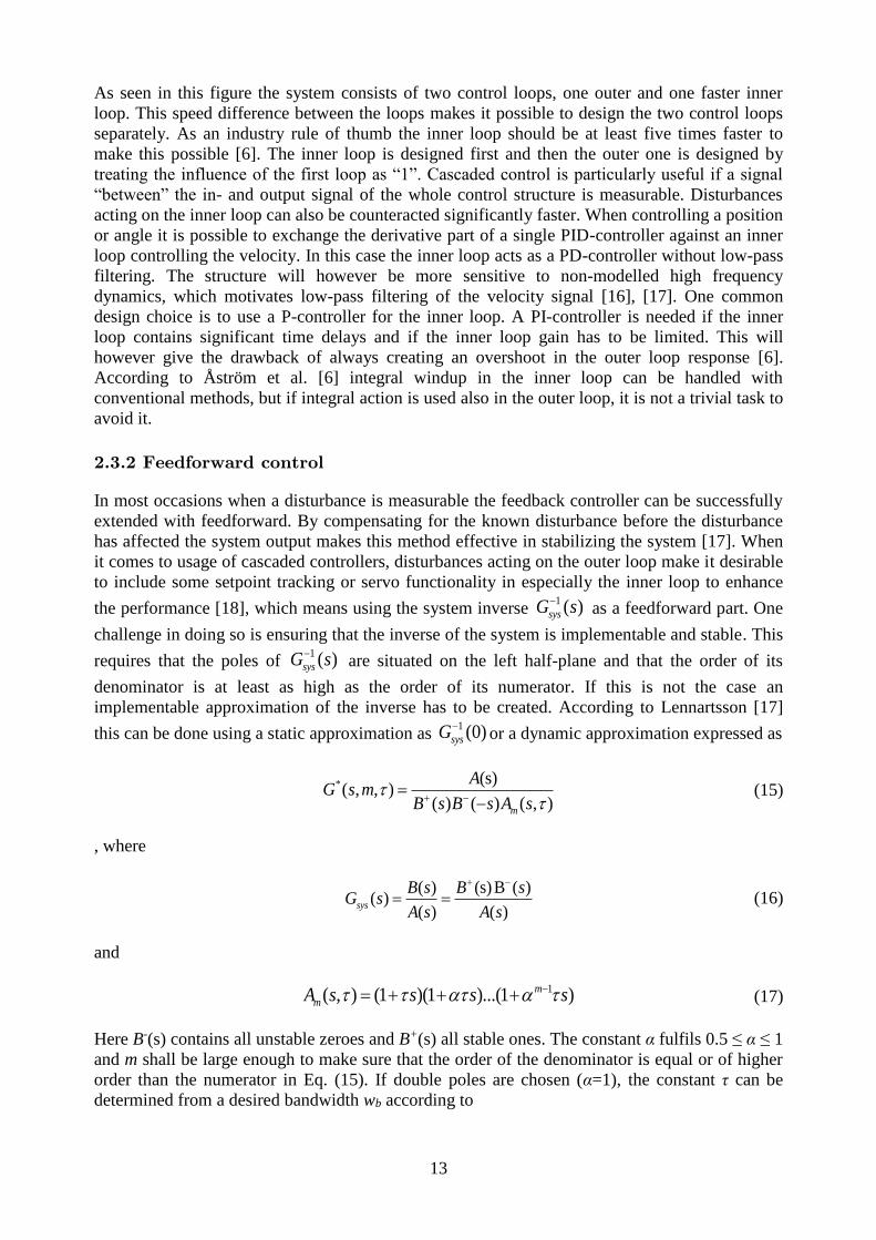
2.3.4 Internal model control

Internal model control (IMC) is a control structure commonly associated with good setpoint

tracking, robustness and efficient tuning, but suffers from slow handling of disturbances [22],

[23] and [24]. The typical IMC-structure is given by Figure 8.

Figure 8. Typical structure of an IMC-controller, where everything inside the dashed lines belongs to the controller.

For the case when ˆ(s) (s)G G perfect setpoint tracking is achieved and the closed-loop transfer

function is Q(s)Gsys(s). In other words, the closed-loop response depends linearly on Q(s). When

the plant model is not perfect the system acts like a feedback system. The first step in the design

process is to factorize the plant as in Eq. (16) and then to define the controller as

1ˆ( ) ( ) ( )Q s G s F s

(20)

, where 1ˆ ( )G s

excludes all unstable zeroes and F(s) is a low pass filter with static gain 1 [24].

The most common choice of F(s) is

1

( )(1 )n

F ss

(21)

, which provides perfect setpoint tracking of step responses, but another common choice is

1

( )(1 )n

n sF s

s

(22)

, in order to get perfect tracking of ramps. Here λ is the closed-loop time constant and n an

integer large enough to make the closed-loop transfer function proper [25]. Even if λ is the only

design parameter of the controller, Kaya [24] proposed a method of choosing λ based on the

open-loop phase and gain margin. If the closed-loop bandwidth is higher than the open-loop one,

Braatz et al. [25] proposed inclusion of lead filters in F(s) to improve the performance. One

requirement of IMC is that the open-loop plant is stable and then the robustness is guaranteed

through reduction of the closed-loop bandwidth [26]. In many papers the IMC-PID structure and

associated tuning process deals with a predefined FOPDT (First-Order Plus Dead Time) model

structure of the plant [22], [23], [24] and [26]. According to Leva [23] it may not be a trivial task

to abandon this predefined structure.

16

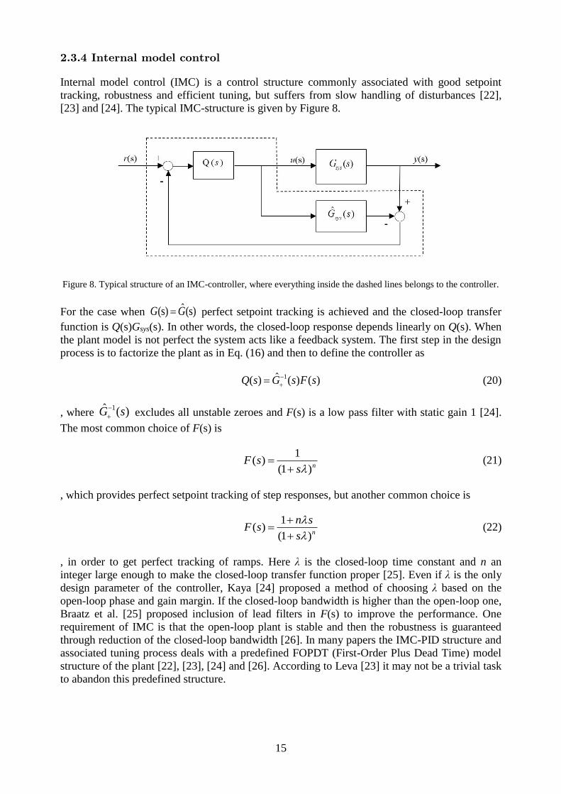
2.3.5 Self-tuning regulators

The self-tuning regulator (STR) attempts to automate several of the controller design steps

consisting of modelling, control law creation, implementation and verification. It can

automatically tune its control parameters in real-time to obtain a desired closed loop response. In

this sense it can also be described as an adaptive controller. In Figure 9 the general structure of

the STR is shown.

Figure 9. Structure of the self-tuning regulator [7].

Basically the STR executes in three steps; system identification based on the measured plant

response, calculation of control parameters based on the system identification and at last

calculation of the control signal based on the control parameters [27]. The control structure can

be viewed as two loops, in where one is the ordinary feedback loop and the other handles the

calculation of control parameters. This three-step controller is sometimes referred to as “explicit”

or “indirect”, because it is also possible to directly estimate the controller parameters in one step,

which is then referred to as “direct” or “implicit” STR.

In the context of STR a wide amount of different underlying estimation and design methods can

be used, but in this section the structure and design procedure proposed in Wittenmark et al. [7]

will be briefly described.

For the parameter estimation of the plant model the earlier presented concept of least squares can

be used. To be able to use it in a STR real-time application, the algorithm however has to be

modified in order to handle sequential access to the in- and output data pairs. The algorithm that

enables this is the recursive least squares (RLS). If the parameters vary with time depending on

the operation condition and if they vary in a smooth manner one approach is to use an extension

called exponential forgetting [7]. With the plant model written as

1 2 0 0 0( ) ( 1) ( 2) ... ( ) ( ) ... ( )

n my t a y t a y t a y t n b u t d b u t d m (23)

, the equations for the recursive least squares with exponential forgetting can be expressed as

17

0 0

1 2 0 1

1

( 1) ( 1) ... ( ) ( ) ... ( )

... ...

( ) ( 1) ( 1)( ( 1) ( 1) ( 1))

ˆ ˆ ˆ( ) ( 1) K(t)(y(t) ( 1) ( 1))

( ) ( ( ) ( 1)) P(t 1) /

T

T

n m

T

T

T

t y t y t n u t d u t d m

a a a b b b

K t P t t t P t t

t t t t

P t I K t t

(24)

This algorithm requires an initial start guess of the parameter vector and a suitable start value

of the covariance matrix P may be a large multiple of the identity matrix. Furthermore I denotes

the identity matrix and the forgetting factor that indirectly determines how many previous

samples the estimate should be based upon. If the value of equals 1, the algorithm will take

all previous values into account and for a value smaller than 1, the algorithm will “forget” old

values. A smaller value will hence make the parameter estimates fluctuate more. One

disadvantage in using the exponential forgetting method is that the parameter estimates are

adjusted even if all elements in ( 1)t equal zero and do not contain any new information. It is

however possible to avoid this using several more complex approaches not only taking the time

into account as discussed in [7] and [28]. Equation (24) also contains an inverse, but since its

argument reduces to a scalar, there is no risk for taking the inverse of a non-singular matrix. One

property of the RLS-algorithm is that it will only converge towards the true parameter values if

the input signal is sufficiently exciting. If the data gathering occurs in a closed loop system and

during operation it can be hard to obtain a persistently exciting input signal. A unique solution of

the parameter estimates may be missing for feedback systems, however this is not a problem for

high order systems or when the controller changes with time. Another requirement to ensure that

the parameters converge towards their true values using least square is that the measurement

noise can be described as white noise.

When it comes to the second and third step in the STR-execution, i.e. to calculate the controller

parameters and the output from the controller, a 2-DOF structure with zero cancellation and

shared denominators according to Figure 10 is proposed in [7].

Figure 10. Controller structure of the proposed self-tuning regulator.

Here the polynomials A and B are assumed to be expressed in the discrete shift operator z and to

not include any common factors (relatively prime). Using the Diophantine equation, pole

placement design can be done based on the closed loop transfer function

(s) ( )BT

y r sAR BS

(25)

Whether model following can be achieved using this structure depends on the model, the system

and on the setpoint. As in Eq. (16) the B polynomial has to be divided into two parts before using

the system inverse. In addition to all unstable zeroes, B- also has to include all poorly damped

18

zeroes that cannot be cancelled. Another restriction is that the B+ and A polynomials must be

monic; i.e. that the highest order should have unity gain.

To be able to cancel the plant zeroes the polynomial B+ has to be included in the closed-loop

characteristic polynomial Ac and in the expression for R as

0

'

c mA A A B

R R B

(26)

This enables a reduction of the Diophantine equation to

'

0 mAR B S A A (27)

, from where the unknown coefficients of R and S can be found. In this context the desired

closed-loop transfer function is assumed to be expressed as Bm/Am and the closed-loop pole

locations specified by A0Am. Furthermore, T can be expressed as

0 mA BT

B (28)

, where Bm should ensure that the closed loop gain is unity. To ensure that the controller is

implementable the causality conditions {deg S ≤ deg R} and {deg T ≤ deg R} must apply. To

obtain the solution with the lowest possible degree and without any unnecessary time delays, the

minimum-degree solution implies

0

deg = deg

deg = deg

deg = deg - deg - 1

m

m

A A

B B

A A B

(29)

For the case when all zeroes are cancelled it is stated as “natural” to choose

0(1) d

m mB A z (30)

, where d0 denotes the pole access of the plant model.

As is discussed in [29], several uncertainties can make it hard to implement a STR, but two

successful implementations in the context of motor control can be found in [27] and [30].

Automatic tuning systems have been developed with the purpose of making it possible for

operators in the industry to tune controllers with a very limited amount of knowledge [20].

19

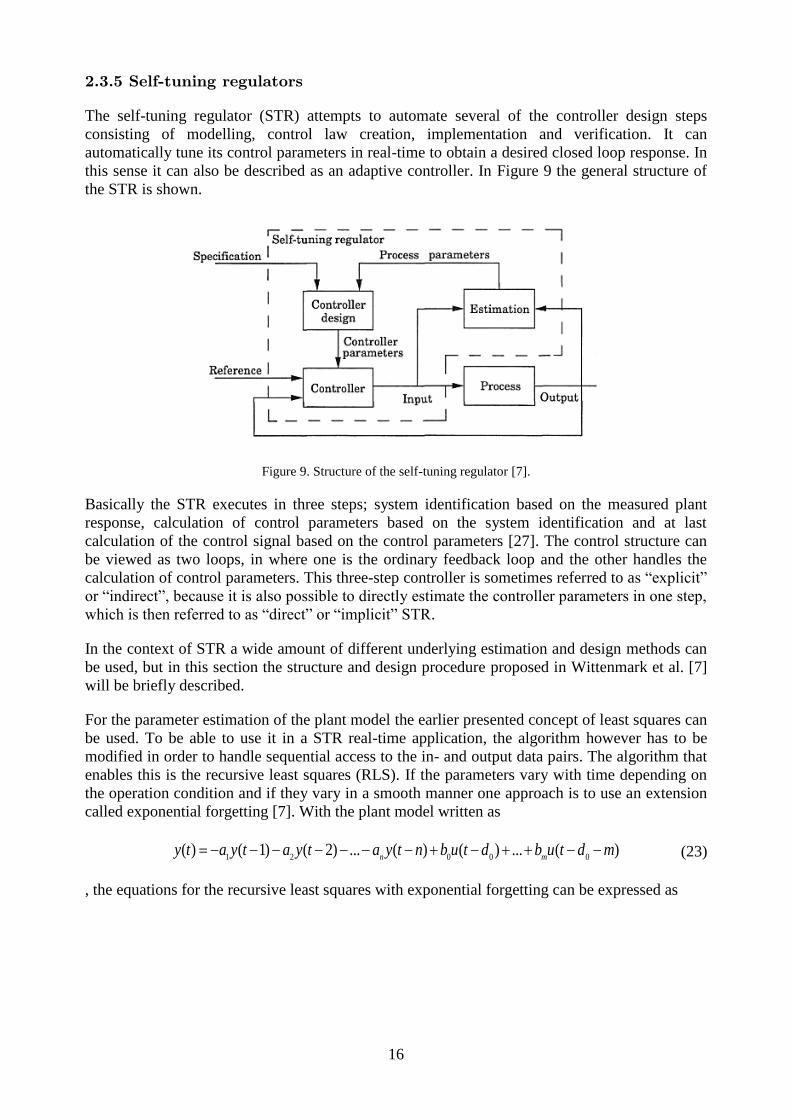
3 PHYSICAL MEASUREMENTS

In order to allow system identification on the real system and verification of the models, some

measurements had to be taken. The tests were carried out on a flat dry road surface at the test

centre Hällered, as seen in Figure 11 to the left, situated east of Gothenburg, Sweden.

Figure 11. The test centre and the vehicle used in the experiment.

To the right in this figure the test vehicle is shown; a Volvo XC90 T6, year 2015, with AWD,

automatic gearbox, a touring chassis, and normal spring dampers, equipped with Pirelli 235/55

R19 tires. The touring chassis specification determines the characteristics of the dampers, coil

springs and the anti-roll bars used.

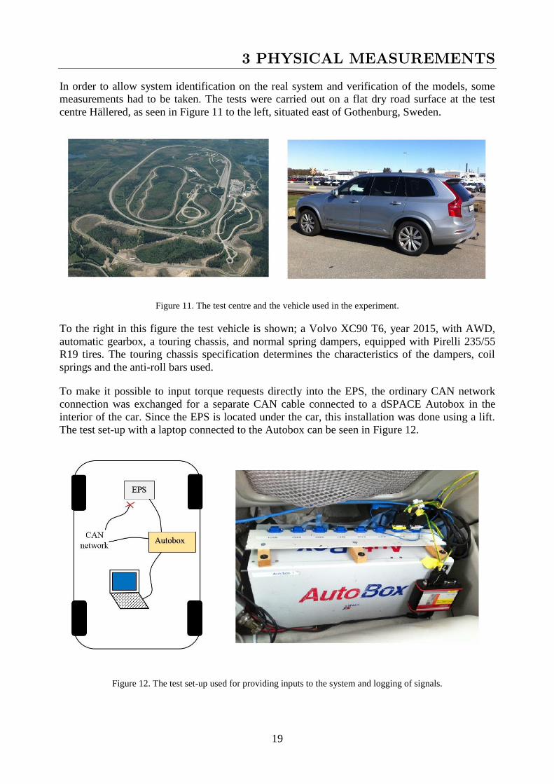
To make it possible to input torque requests directly into the EPS, the ordinary CAN network

connection was exchanged for a separate CAN cable connected to a dSPACE Autobox in the

interior of the car. Since the EPS is located under the car, this installation was done using a lift.

The test set-up with a laptop connected to the Autobox can be seen in Figure 12.

Figure 12. The test set-up used for providing inputs to the system and logging of signals.

20

With the software Control Desk running on the laptop, several test cases could be fed into the

EPS and the desired signals could be logged since they were all available on the CAN network.

The longitudinal velocity in each case was regulated by the built-in adaptive cruise controller. As

the EPS interface by default enabled pinion angle request input and not steer torque input, the

STM functionality was temporarily switched off by modifying some specific register bits with

help from the software CANape.

In the first test case a series of torque step inputs of different magnitudes were used and the

resulting pinion angle and pinion angle rate were logged. Both the pinion angle and the pinion

angle rate are calculated and measured with high accuracy by an existing encoder in the EPS.

Due to safety limitations low vehicle speeds and torques were used. In Table 3 the details of the

test cases are summarized.

Table 3. Description of the test cases used.

Test

case

Vehicle

speed [kph]

Input signal Measured output

signals

1 30 EPS torque request [Nm] using several step inputs with

magnitudes [0.1 0.2 0.3 0.4 0.5] Nm.

Pinion angle [deg] and

pinion angular velocity

[deg/s].

2 0, 5, 10, 25,

50

EPS torque request [Nm] using a continuous sinus wave with a

fixed amplitude of 0.5 Nm and with an increasing frequency

ranging from 0.6 Hz up to 20 Hz (sine sweep).

Pinion angle [deg] and

pinion angular velocity

[deg/s].

In the second test case a sinusoidal torque input was used with increasing frequency in order to

excite the whole frequency spectrum of the system. A set of different vehicle speeds were used,

in order to illustrate the speed dependence (even if this knowledge already existed at the

department). With a sample time of 10 ms the Nyquist frequency will be 50 Hz. This value will

hence equal the theoretical maximum frequency that can be identified from the measurements. In

reality it is usually recommended to have some more margin to this value. The experiment with a

sinusoidal input was therefore performed up to a frequency of 20 Hz, due to this constraint and

due previous experience at the department. According to a development engineer similar tests

have been made up to around 30 Hz, but the measured data above 20 Hz tended to be greatly

influenced by noise and to have a low gain. Independent information from the vehicle dynamics

department, based on previous experience, also states that frequencies above around 20 Hz,

resulting from the dynamics of the car are mainly damped out by the tires etc. This justifies the

choice of limiting the relevant frequency range up to 20 Hz.

21

4 MODELLING

This chapter focuses on the modelling of the system, where two complete vehicle models are

described, which originates from existing material at Volvo Cars.

4.1 Description of models

From Section 2.2 it has been concluded that a full vehicle model together with the geometry of

the steering and suspension system is needed. One identified important feature of the model if it

should be used in the design and tuning of the STM, is also that it can be easily adapted to new

car models. Since a full vehicle model contains a large amount of parameters, this requirement

makes it advantageous to make use of a model that is already used and maintained by the vehicle

dynamics department. More detailed modelling (than in Section 2.2) may be required and by

making use of existing material a higher goal can be reached. With this background an existing

model created in the software CarMaker and Matlab/Simulink was found suitable to use in this

thesis. A co-simulation model built upon existing models in Adams and Simulink has also been

created and evaluated to see if sufficient simulation accuracy can be reached.

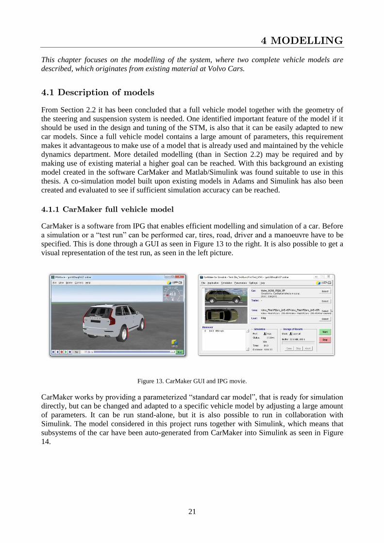
4.1.1 CarMaker full vehicle model

CarMaker is a software from IPG that enables efficient modelling and simulation of a car. Before

a simulation or a “test run” can be performed car, tires, road, driver and a manoeuvre have to be

specified. This is done through a GUI as seen in Figure 13 to the right. It is also possible to get a

visual representation of the test run, as seen in the left picture.

Figure 13. CarMaker GUI and IPG movie.

CarMaker works by providing a parameterized “standard car model”, that is ready for simulation

directly, but can be changed and adapted to a specific vehicle model by adjusting a large amount

of parameters. It can be run stand-alone, but it is also possible to run in collaboration with

Simulink. The model considered in this project runs together with Simulink, which means that

subsystems of the car have been auto-generated from CarMaker into Simulink as seen in Figure

14.

22

Figure 14. Structure of the CarMaker model after integration into Simulink.

Within this structure it is possible to exchange certain subsystems for Simulink models delivered

from different sub-suppliers for example. To make the simulation as fast as possible the

CarMaker brake and powertrain subsystems were not exchanged in the final set-up, because they

do not affect the lateral movement of the car when a constant vehicle speed is used. One

subsystem of greater importance for this application that had been exchanged was the electric

power steering system. This subsystem is delivered from a sub-supplier and is coloured light

blue in Figure 15, where it is implemented together with the CarMaker model.

Figure 15. The Simulink EPS model integrated together with CarMaker.

In this figure it is also possible to see the verification setup later used in the evaluation of the

model. The EPS-model comprises the rack, the rack and pinion gear, the servo gear (belt and ball

nut gear), the electrical motor and all software functions in the controlling ECU. For each

mechanical part, friction, stiffness, inertia/mass and efficiency are included. It can be adapted to

handle both fixed-time step solvers (simplified) and variable-time step solvers. For the CarMaker

setup a fixed-time step of 1 ms was used.

Since the ordinary usage of the model meant inputting a driver steering angle into the Simulink

model from the CarMaker GUI, the model had to be slightly modified in order to be able to

handle torque inputs. This was done by adding a dynamic equation for the steering column. With

this equation the torque from the torsion bar TTB calculated by the EPS-model, together with a

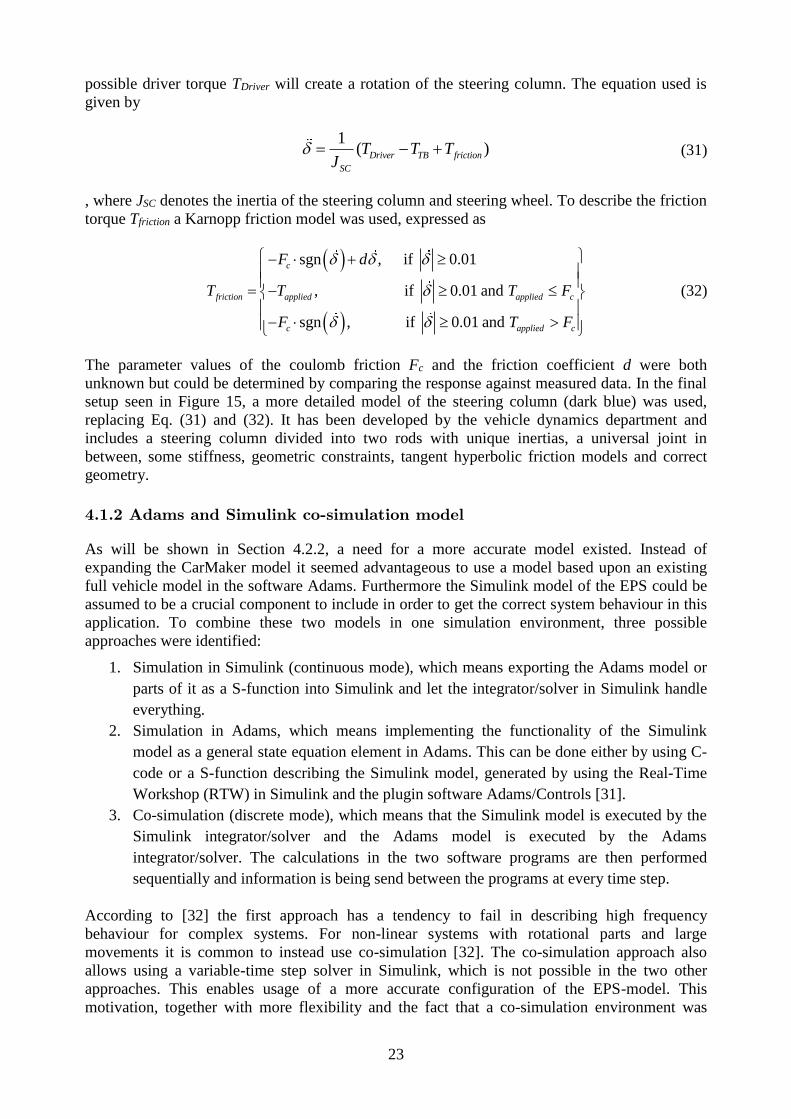
23

possible driver torque TDriver will create a rotation of the steering column. The equation used is

given by

1

( )Driver TB friction

SC

T T TJ

(31)

, where JSC denotes the inertia of the steering column and steering wheel. To describe the friction

torque Tfriction a Karnopp friction model was used, expressed as

sgn , if 0.01

, if 0.01 and

sgn , if 0.01 and

c

friction applied applied c

c applied c

F d

T T T F

F T F

(32)

The parameter values of the coulomb friction Fc and the friction coefficient d were both

unknown but could be determined by comparing the response against measured data. In the final

setup seen in Figure 15, a more detailed model of the steering column (dark blue) was used,

replacing Eq. (31) and (32). It has been developed by the vehicle dynamics department and

includes a steering column divided into two rods with unique inertias, a universal joint in

between, some stiffness, geometric constraints, tangent hyperbolic friction models and correct

geometry.

4.1.2 Adams and Simulink co-simulation model

As will be shown in Section 4.2.2, a need for a more accurate model existed. Instead of

expanding the CarMaker model it seemed advantageous to use a model based upon an existing

full vehicle model in the software Adams. Furthermore the Simulink model of the EPS could be

assumed to be a crucial component to include in order to get the correct system behaviour in this

application. To combine these two models in one simulation environment, three possible

approaches were identified:

1. Simulation in Simulink (continuous mode), which means exporting the Adams model or

parts of it as a S-function into Simulink and let the integrator/solver in Simulink handle

everything.

2. Simulation in Adams, which means implementing the functionality of the Simulink

model as a general state equation element in Adams. This can be done either by using C-

code or a S-function describing the Simulink model, generated by using the Real-Time

Workshop (RTW) in Simulink and the plugin software Adams/Controls [31].

3. Co-simulation (discrete mode), which means that the Simulink model is executed by the

Simulink integrator/solver and the Adams model is executed by the Adams

integrator/solver. The calculations in the two software programs are then performed

sequentially and information is being send between the programs at every time step.

According to [32] the first approach has a tendency to fail in describing high frequency

behaviour for complex systems. For non-linear systems with rotational parts and large

movements it is common to instead use co-simulation [32]. The co-simulation approach also

allows using a variable-time step solver in Simulink, which is not possible in the two other

approaches. This enables usage of a more accurate configuration of the EPS-model. This

motivation, together with more flexibility and the fact that a co-simulation environment was

24

being prepared by the vehicle dynamics department at Volvo Cars simultaneously, made the co-

simulation concept the best choice for further evaluations. Examples of earlier successful co-

simulation projects that were also considered include [33] and [34].

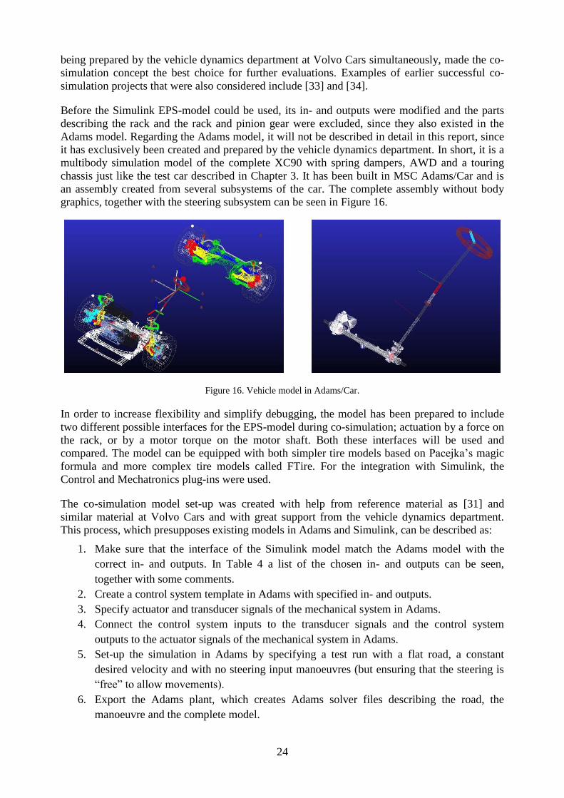
Before the Simulink EPS-model could be used, its in- and outputs were modified and the parts

describing the rack and the rack and pinion gear were excluded, since they also existed in the

Adams model. Regarding the Adams model, it will not be described in detail in this report, since

it has exclusively been created and prepared by the vehicle dynamics department. In short, it is a

multibody simulation model of the complete XC90 with spring dampers, AWD and a touring

chassis just like the test car described in Chapter 3. It has been built in MSC Adams/Car and is

an assembly created from several subsystems of the car. The complete assembly without body

graphics, together with the steering subsystem can be seen in Figure 16.

Figure 16. Vehicle model in Adams/Car.

In order to increase flexibility and simplify debugging, the model has been prepared to include

two different possible interfaces for the EPS-model during co-simulation; actuation by a force on

the rack, or by a motor torque on the motor shaft. Both these interfaces will be used and

compared. The model can be equipped with both simpler tire models based on Pacejka’s magic

formula and more complex tire models called FTire. For the integration with Simulink, the

Control and Mechatronics plug-ins were used.

The co-simulation model set-up was created with help from reference material as [31] and

similar material at Volvo Cars and with great support from the vehicle dynamics department.

This process, which presupposes existing models in Adams and Simulink, can be described as:

1. Make sure that the interface of the Simulink model match the Adams model with the

correct in- and outputs. In Table 4 a list of the chosen in- and outputs can be seen,

together with some comments.

2. Create a control system template in Adams with specified in- and outputs.

3. Specify actuator and transducer signals of the mechanical system in Adams.

4. Connect the control system inputs to the transducer signals and the control system

outputs to the actuator signals of the mechanical system in Adams.

5. Set-up the simulation in Adams by specifying a test run with a flat road, a constant

desired velocity and with no steering input manoeuvres (but ensuring that the steering is

“free” to allow movements).

6. Export the Adams plant, which creates Adams solver files describing the road, the

manoeuvre and the complete model.

25

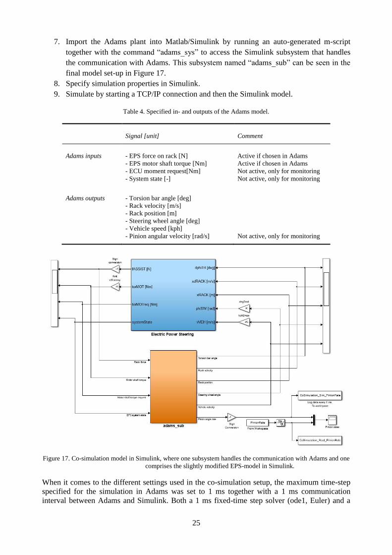
7. Import the Adams plant into Matlab/Simulink by running an auto-generated m-script

together with the command “adams_sys” to access the Simulink subsystem that handles

the communication with Adams. This subsystem named “adams_sub” can be seen in the

final model set-up in Figure 17.

8. Specify simulation properties in Simulink.

9. Simulate by starting a TCP/IP connection and then the Simulink model.

Table 4. Specified in- and outputs of the Adams model.

Signal [unit] Comment

Adams inputs - EPS force on rack [N]

- EPS motor shaft torque [Nm]

- ECU moment request[Nm]

- System state [-]

Active if chosen in Adams

Active if chosen in Adams

Not active, only for monitoring

Not active, only for monitoring

Adams outputs - Torsion bar angle [deg]

- Rack velocity [m/s]

- Rack position [m]

- Steering wheel angle [deg]

- Vehicle speed [kph]

- Pinion angular velocity [rad/s]

Not active, only for monitoring

Figure 17. Co-simulation model in Simulink, where one subsystem handles the communication with Adams and one

comprises the slightly modified EPS-model in Simulink.

When it comes to the different settings used in the co-simulation setup, the maximum time-step

specified for the simulation in Adams was set to 1 ms together with a 1 ms communication

interval between Adams and Simulink. Both a 1 ms fixed-time step solver (ode1, Euler) and a

26

variable-time step solver (ode15s, stiff/NDF) for the EPS Simulink model have been evaluated.

These two different settings corresponds to the recommended solver settings for the EPS model,

as could be found in the documentation from the sub-supplier. To avoid algebraic loops or usage

of unit delay blocks, Adams was set to “lead” the simulation with Simulink following using its

outputs. Interpolation and extrapolation of the signals passed between the programs was tried but

not used, since it did not improve or speed up the simulations. TCP/IP based communication was

used between Adams and Matlab, since the preparations for this were already done.

Initially, the largest issue with the model was the long simulation time. A simulation of 74

seconds that excites the complete frequency range of interest took over 24 hours even though the

simulation mode in Adams was set to “files only” (batch mode simulation and no interactive

simulation with graphics) and with an update of the Adams output files once every 10 ms instead

of every 1 ms (setting the parameter “Number of communications per output step”=10 inside the

adams_sub block). The solution to this was to disregard the results from Adams, either by only

updating the files once every second or by completely exclude the result file (by modifying the

generated .adm-file). This resulted in simulation times around 80 minutes for a 74 second

simulation with much dynamics.

4.2 Model evaluations

In this section the accuracy of the models are evaluated with help from the data gathered during

the physical measurements. Requirements for the model is also elaborated from physical

measurements and later in a sensitivity analysis.

4.2.1 Model requirements derived from the system

To start with, it can be clarified that a model used in the development of the STM-controller can

be useful both in the design and in the verification of the controller. As described in Section

1.1.2, the currently used controller utilizes an inverse filter derived from a system identification

of the real plant. If it is possible to perform this system identification using a virtual model

instead of using a development vehicle, it would be extremely valuable. This will however put

high demands on the model regarding accuracy. For STM simulation and verification purposes

the usage of a model is more obvious.

One important aspect to investigate in this context is how fast dynamics a model is required to

handle accurately. This requirement may differ slightly depending on the user case. The

bandwidth of the model, here defined as the frequency range were the model is able to describe

the real system behaviour (with some fault margin), that is required for simulation purposes can

be determined by investigating the characteristics of the STM output. Based on driver comfort

measurements, the derivative of the torque output is limited and this maximal value is correlated

with a maximum frequency, with which the controller output will excite the model. By studying

the frequency content in the torque signal from the STM some knowledge may therefore be

gathered. For this study earlier logged data obtained during real operating situations on

expeditions performed on roads in Europe were used. A large amount of log files were scanned

for events of automatic steering interventions, using functionality available at the department.

Four files containing a high rate of steering interventions were then retrieved. From these, the

relevant signal was located and analysed with the discrete Fourier transform, computed with the

fast Fourier transform algorithm in Matlab. The result is illustrated in Figure 18.

27

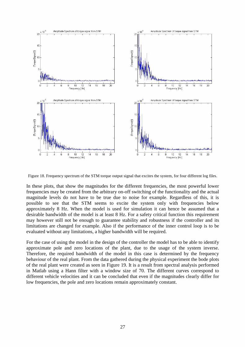
Figure 18. Frequency spectrum of the STM torque output signal that excites the system, for four different log files.

In these plots, that show the magnitudes for the different frequencies, the most powerful lower

frequencies may be created from the arbitrary on-off switching of the functionality and the actual

magnitude levels do not have to be true due to noise for example. Regardless of this, it is

possible to see that the STM seems to excite the system only with frequencies below

approximately 8 Hz. When the model is used for simulation it can hence be assumed that a

desirable bandwidth of the model is at least 8 Hz. For a safety critical function this requirement

may however still not be enough to guarantee stability and robustness if the controller and its

limitations are changed for example. Also if the performance of the inner control loop is to be

evaluated without any limitations, a higher bandwidth will be required.

For the case of using the model in the design of the controller the model has to be able to identify

approximate pole and zero locations of the plant, due to the usage of the system inverse.

Therefore, the required bandwidth of the model in this case is determined by the frequency

behaviour of the real plant. From the data gathered during the physical experiment the bode plots

of the real plant were created as seen in Figure 19. It is a result from spectral analysis performed

in Matlab using a Hann filter with a window size of 70. The different curves correspond to

different vehicle velocities and it can be concluded that even if the magnitudes clearly differ for

low frequencies, the pole and zero locations remain approximately constant.

28

Figure 19. Bode diagrams of the plant from torque (Nm) to pinion angular velocity (rad/s).

It can be seen that there exists a significant resonance frequency at around 88 rad/s (14 Hz) and

one at around 19 rad/s (3 Hz). With respect to this it can be concluded that the required

bandwidth of the model in the case of controller design has to be approximately 100 rad/s (16

Hz). According to [29] the model has to be accurate at least for frequencies where the loop gain

is around unity to enable robust controller design when using model following. This statement is

understandable and is in line with the previous conclusion.

Important model requirements can also be derived from an understanding about which

subsystems and parameters that have the largest effect on the system response. From this

knowledge it is possible to provide guidelines for the required complexity of the different parts

of the model. To utilize some of the great amount of existing knowledge at the vehicle dynamics

department, several interviews were carried out. From these interviews it was concluded that the

system response illustrated in Figure 19 showed large similarities to the vertical dynamics of the

car during brake and steering manoeuvres. Hence a natural hypothesis is that these responses are

correlated and affected by the same subcomponents to a certain extent. The components that

have the most influence on the first vertical resonance frequency around 3 Hz are the dampers of

the car.

When it comes to the higher resonance frequency around 14 Hz, the tires with a significantly

more stiff behaviour, are probably among the most important contributors according to different

sources at the vehicle dynamics department. This statement seems also valid according to an

earlier test performed at the active safety department. In this test, the system response between

applied torque into the EPS and measured angular velocity of the pinion was evaluated for two

tires that differed significantly (a “standard” tire and a low-profile tire). The conclusion was that

29

the system response does not change significantly when using different tires and that the tires

mainly affect the high frequency behaviour. Some of this data is illustrated in Appendix B.

4.2.2 CarMaker model evaluation

The dynamic behaviour between applied steering torque in the EPS and the resulting pinion

angle response has not been verified in the CarMaker model earlier and the model has not been

used within the field of active safety before. This made it necessary to verify that the model

could collaborate with the STM and that it was sufficiently accurate for this purpose.

As concluded in the previous section it is important that the model is accurate in a frequency

range up to at least 16 Hz. With the sinusoidal torque input signal used during the experiment,

the pinion angle rates produced by the model was compared with the real measurements. For low

frequencies the simulation model produced very good results, as can be seen in Figure 20, with

good amplitude and friction levels.

Figure 20. Comparison between CarMaker simulation and measured pinion angle rate for a vehicle speed of 50

km/h. The input is a low frequency sinusoidal torque into the EPS-system.

To evaluate the performance of the CarMaker model in the complete range of interesting

frequencies, spectral analysis of both the measured and the simulated signals were performed.

This analysis was performed in Matlab with a Hann window. A large window size of 100 was

used (small in time domain), since it gave a more true representation of the data, without giving

problems with noise variations. The data was then represented in bode plots, Figure 21, where it

can be concluded that the model accuracy for low frequencies is very good. In addition the first

resonance peak is also present in the model, but at a slightly higher frequency. For higher

frequencies, above 3 Hz (20 rad/s), the model lacks accuracy both in terms of phase shift and

gain. With respect to this, it seems possible to get an estimation of the real pole and zero

locations using the model for the lower frequencies, but not for the higher frequencies.

30

Figure 21. Comparison between CarMaker simulation and measured pinion angle rate for a vehicle speed of 50

km/h.

Possible explanations for this can partly originate from the tire model PAC2002 that is used in

the model, which is based on the magic formula. This model, according to the tire engineers at

Volvo Cars, only describes the correct behaviour of the tires up to approximately 8 Hz. Other tire

models used at Volvo Cars that perform better when it comes to high frequencies are the so

called SWIFT (designed to handle frequencies up to at least 70 Hz [35]) and the FTire model

(designed to handle frequencies up to at least 120 Hz [36]). These models were however at the

moment not possible to implement in CarMaker due to incompleteness or practical issues.

If the model is to be used together with the STM in simulations, it is also of interest how well it

can replicate step responses. In Figure 22, both the angle response and the angle rate response for

two different torque step inputs are shown. From these plots it can be concluded that model

performance for the larger step of 0.5 Nm is satisfying, but for the smaller step the performance

is less accurate. This can be due to some nonlinearities not captured by the model.

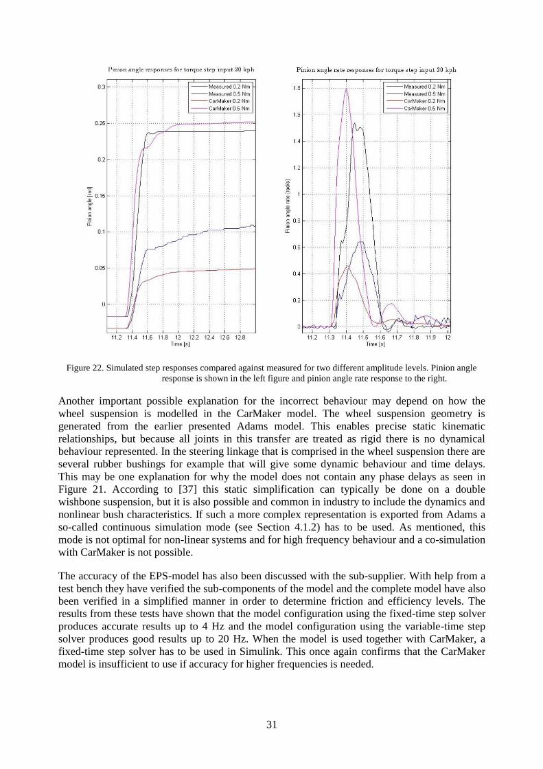
31

Figure 22. Simulated step responses compared against measured for two different amplitude levels. Pinion angle

response is shown in the left figure and pinion angle rate response to the right.

Another important possible explanation for the incorrect behaviour may depend on how the

wheel suspension is modelled in the CarMaker model. The wheel suspension geometry is

generated from the earlier presented Adams model. This enables precise static kinematic

relationships, but because all joints in this transfer are treated as rigid there is no dynamical

behaviour represented. In the steering linkage that is comprised in the wheel suspension there are

several rubber bushings for example that will give some dynamic behaviour and time delays.

This may be one explanation for why the model does not contain any phase delays as seen in

Figure 21. According to [37] this static simplification can typically be done on a double

wishbone suspension, but it is also possible and common in industry to include the dynamics and

nonlinear bush characteristics. If such a more complex representation is exported from Adams a

so-called continuous simulation mode (see Section 4.1.2) has to be used. As mentioned, this

mode is not optimal for non-linear systems and for high frequency behaviour and a co-simulation

with CarMaker is not possible.

The accuracy of the EPS-model has also been discussed with the sub-supplier. With help from a

test bench they have verified the sub-components of the model and the complete model have also

been verified in a simplified manner in order to determine friction and efficiency levels. The

results from these tests have shown that the model configuration using the fixed-time step solver

produces accurate results up to 4 Hz and the model configuration using the variable-time step

solver produces good results up to 20 Hz. When the model is used together with CarMaker, a

fixed-time step solver has to be used in Simulink. This once again confirms that the CarMaker

model is insufficient to use if accuracy for higher frequencies is needed.

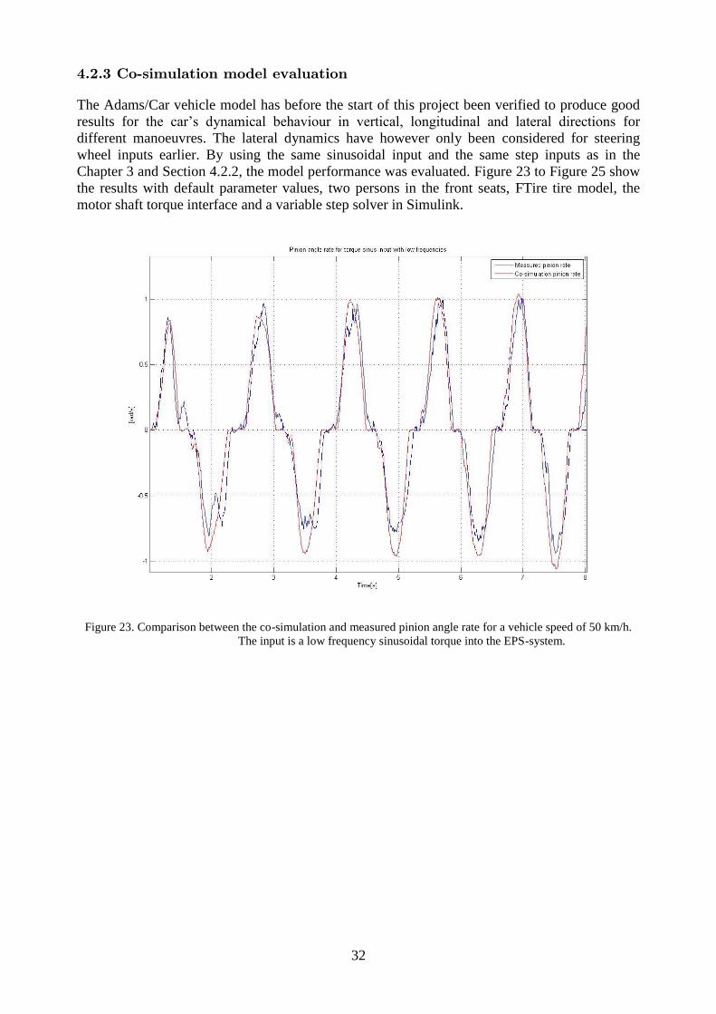
32

4.2.3 Co-simulation model evaluation

The Adams/Car vehicle model has before the start of this project been verified to produce good

results for the car’s dynamical behaviour in vertical, longitudinal and lateral directions for

different manoeuvres. The lateral dynamics have however only been considered for steering

wheel inputs earlier. By using the same sinusoidal input and the same step inputs as in the

Chapter 3 and Section 4.2.2, the model performance was evaluated. Figure 23 to Figure 25 show

the results with default parameter values, two persons in the front seats, FTire tire model, the

motor shaft torque interface and a variable step solver in Simulink.

Figure 23. Comparison between the co-simulation and measured pinion angle rate for a vehicle speed of 50 km/h.

The input is a low frequency sinusoidal torque into the EPS-system.

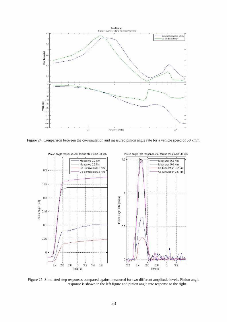
33

Figure 24. Comparison between the co-simulation and measured pinion angle rate for a vehicle speed of 50 km/h.

Figure 25. Simulated step responses compared against measured for two different amplitude levels. Pinion angle

response is shown in the left figure and pinion angle rate response to the right.

34

In Figure 23, one can see that the low frequency model behaviour is as good as for the CarMaker

model shown in Figure 20, for example static friction levels seem to be correct. Regarding the

complete frequency range in Figure 24, the co-simulation model shows a significantly better

accuracy, where both of the resonance frequencies and the zero in the amplitude dip are present.

Notably however is that the first resonance frequency appears at a slightly lower frequency for

the co-simulation model compared to the real system. Figure 25 shows that the step response for

the larger step correlates well with the measure step, but for a smaller step the correlation is not

as good. In this matter the co-simulation model shows similar tendencies as the CarMaker

model. Known differences between the test car and the Adams/Car model that may not have a

negligible influence include:

In Adams/Car 235/60 R18 tires were used instead of the 235/55 R19 tires mounted on the

test vehicle (because the same dimensions were not available)

Not 100 % correct vehicle load/mass. The correct load on the front and rear wheel axis

could have been measured and specified in Adams/Car

For the motor shaft torque interface the inertia of the ball nut screw is approximated, the

cog belt assumed stiff and frictions in the motor and ball nut gear neglected

Not 100 % correct inertia of steering wheel due to differences in the airbag setup between

test vehicle and simulation model

4.2.4 Sensitivity analysis

In order to enlarge the knowledge of the parameters influencing the system response, a

sensitivity analysis was performed on the co-simulation model. This analysis also aimed to give

information about which parameters to vary in tuning the model against the measurements and to

give information about the model requirements in terms of level of detail.

There exists a wide range of different sensitivity analyse methods where literature as [38]

provides guidance. For this specific application, no information exists about the distribution or

uncertainty of the parameters to be varied. All parameters have defined values, from now on

referred to as “default” values, which have been identified before the start of this project. With

respect to this, local methods were deemed most appropriate to use. The complexity of the model

will make analytical methods based on partial derivatives impossible and a limited amount of

time together with long simulation times created the need for a simple and efficient method. On

this basis the One-At-a-Time (OAT) analysis was found suitable, which has been employed in a

wide range of publications like in [39] for example and concluded as appropriate for similar use

by Hamby [40]. This method means neglecting the model interactions and changing one

parameter/factor at a time while keeping all other parameters on their default values. In case of

simulation error it is also easy to find the root cause of the failure.

The default parameter values were modified with ±20 % and the parameters’ influence were

ranked based on how much the resulting pinion angle rate peak value differed. As input a torque

step of 0.5 Nm was used and the vehicle speed was set to be 30 km/h.

In order to get a deeper understanding of the effect of different parameters and model setups on

the dynamics seen in Figure 24, several simulations covering the complete frequency span were

also performed with different settings. Visual inspection of the bode plots was used in order to

gather qualitative data. Influences on the location of the resonance frequencies was of particular

interest. Most of the plots and the quantitative sensitivity analysis results can be found in

Appendix C, but the findings can be summarized here as:

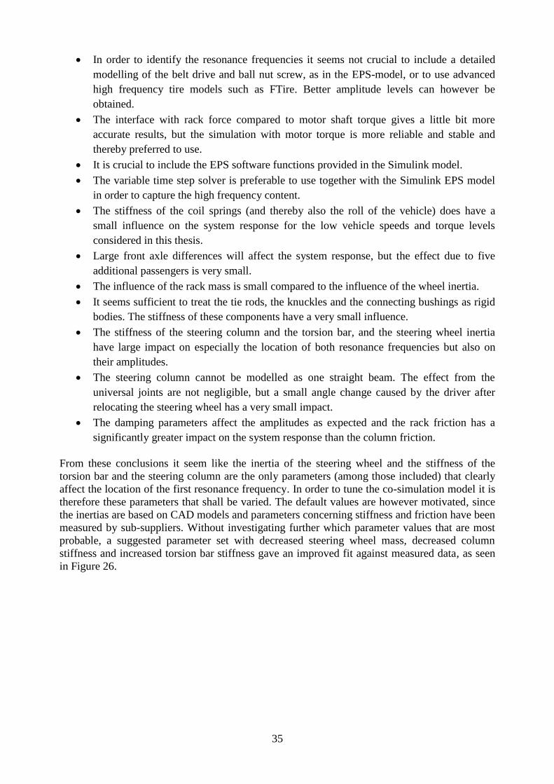
35

In order to identify the resonance frequencies it seems not crucial to include a detailed

modelling of the belt drive and ball nut screw, as in the EPS-model, or to use advanced

high frequency tire models such as FTire. Better amplitude levels can however be

obtained.

The interface with rack force compared to motor shaft torque gives a little bit more

accurate results, but the simulation with motor torque is more reliable and stable and

thereby preferred to use.

It is crucial to include the EPS software functions provided in the Simulink model.

The variable time step solver is preferable to use together with the Simulink EPS model

in order to capture the high frequency content.

The stiffness of the coil springs (and thereby also the roll of the vehicle) does have a

small influence on the system response for the low vehicle speeds and torque levels

considered in this thesis.

Large front axle differences will affect the system response, but the effect due to five

additional passengers is very small.

The influence of the rack mass is small compared to the influence of the wheel inertia.

It seems sufficient to treat the tie rods, the knuckles and the connecting bushings as rigid

bodies. The stiffness of these components have a very small influence.

The stiffness of the steering column and the torsion bar, and the steering wheel inertia

have large impact on especially the location of both resonance frequencies but also on

their amplitudes.

The steering column cannot be modelled as one straight beam. The effect from the

universal joints are not negligible, but a small angle change caused by the driver after

relocating the steering wheel has a very small impact.

The damping parameters affect the amplitudes as expected and the rack friction has a

significantly greater impact on the system response than the column friction.

From these conclusions it seem like the inertia of the steering wheel and the stiffness of the

torsion bar and the steering column are the only parameters (among those included) that clearly

affect the location of the first resonance frequency. In order to tune the co-simulation model it is

therefore these parameters that shall be varied. The default values are however motivated, since

the inertias are based on CAD models and parameters concerning stiffness and friction have been

measured by sub-suppliers. Without investigating further which parameter values that are most

probable, a suggested parameter set with decreased steering wheel mass, decreased column

stiffness and increased torsion bar stiffness gave an improved fit against measured data, as seen

in Figure 26.

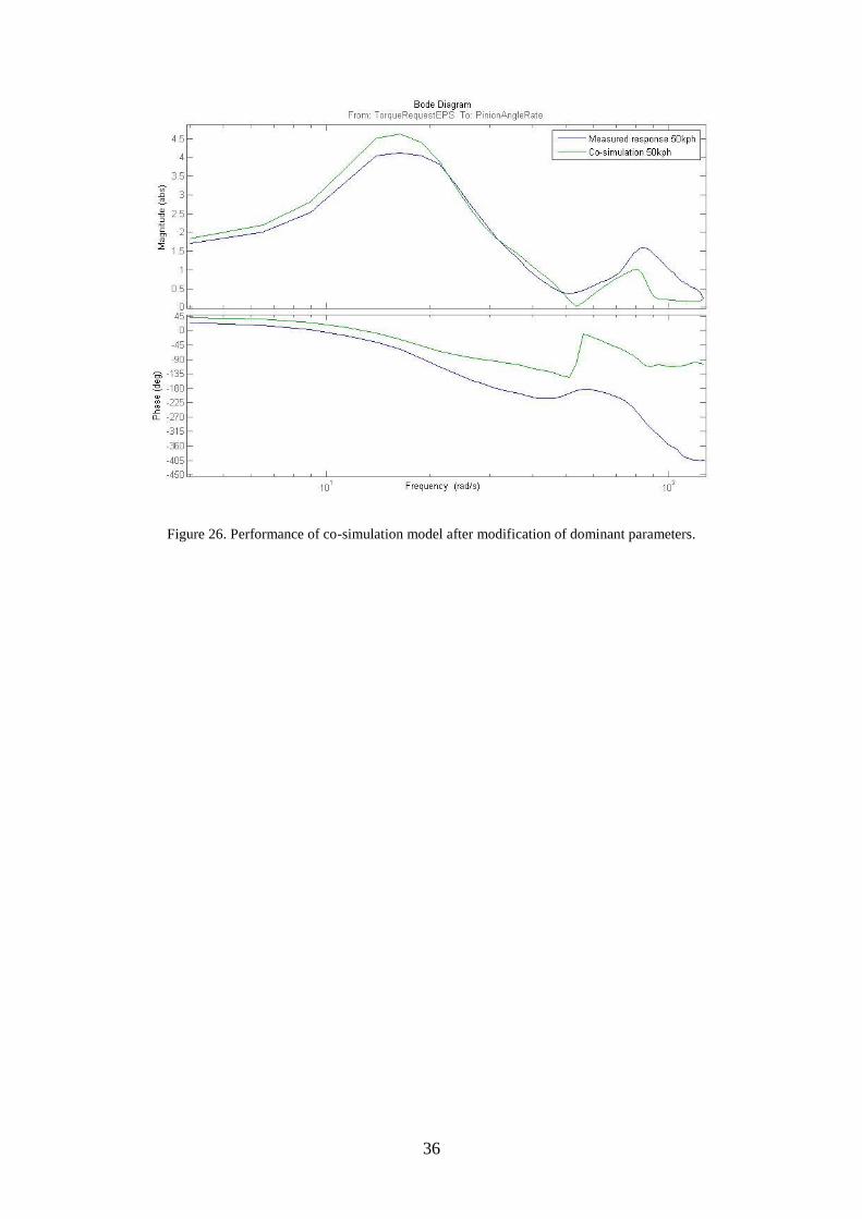
36

Figure 26. Performance of co-simulation model after modification of dominant parameters.

37

5 CONTROL

In this chapter the control investigation is described. To start with the implementations are

presented and then the results.

5.1 Control implementations

The cascaded structure was deemed advantageous to keep since it enables limitation of the

pinion angle rate and as earlier mentioned the study will focus on the STM inner loop. In Section

2.3 the basics of 2-DOF control, IMC and the STR are outlined. These three control concepts

were concluded as promising for reducing the tuning effort. In this section, the implementation

of these are described together with a section evaluating efficient system identification.

5.1.1 System identification

One step in the design of the current controller that was especially time consuming was deriving

the system inverse and therefore this step deserves some attention. If it is possible to create the

inverse more efficiently, time can be spared. One question of interest is if the parameterized

model must have a 6th order numerator and denominator. The recursive least squares algorithm

was also evaluated against other methods, since the STR requires real-time system identification.

All identification was based on the data gathered from the experiment with sinusoidal torque

input and pinion angle rate as output for a vehicle velocity of 25 km/h. After some iterations with

different model orders it was concluded that a discrete model consisting of a 3 or 4-degree

numerator and a 5-degree denominator was sufficient in capturing the essential dynamics shown

in the bode plots of the plant. Three different identification methods were tried; the Output-error

structure, a subspace algorithm for state space system identification and a transfer function

estimation, all methods easily computed with help from Matlab functions. A comparison

between the resulting parameterized models, the existing 6-degree plant model and the real plant

is given in Figure 27.

38

Figure 27. Comparison of three system identification methods, the existing 6-degree model and the real system for

the vehicle speed 25 km/h.

In this figure it can be concluded that the lower order polynomials are able to match the

performance of the higher order model. To be able to use cancellation of the plant zeroes, the

zeroes have to be stable and well-damped. For the model estimated using the subspace algorithm

one unstable zero existed. Two different solutions to this non-minimum phase zero were

evaluated in the continuous domain; i.e. exclusion of the zero together with recalculation of the

static gain (identical behaviour up to 90 Hz) and exchanging the zero to its minimum phase

equivalent as proposed in Eq. (15) (which gives a phase shift). When both models were

translated back to the discrete domain a zero reappeared on the border to instability. This

problem was solved by performing the non-minimum phase handling directly in the discrete

domain. The resulting model can then be expressed as

3 2

5 4 3 2

0.309 0.721 0.597 0.179

3.92 6.61 6.13 3.12 0.685sys

z z zG

z z z z z

(33)

The model derived from the transfer function estimator in Figure 27 seems to give slightly better

performance than the state space identified model, but it suffers from poorly damped zeroes with

a relative damping of ζ = 0.21. For the model in Eq. (33), the relative damping of the most

oscillating zeroes are not optimal either, but a bit better with a value of ζ = 0.43 (equivalent to

the existing model). Poorly damped cancelled zeroes can decrease the performance and make the

control signal oscillatory.

Also a recursive least square (RLS) estimation as proposed in [7] was derived. To lower the risk

for getting a non-minimum phase zero a 3-degree numerator and a 5-degree denominator was

used for the RLS estimation. The algorithm in Eq. (24) was used and a verification of the result

for λ = 1 was done by comparing against output produced by the LS-method in Eq. (2). For

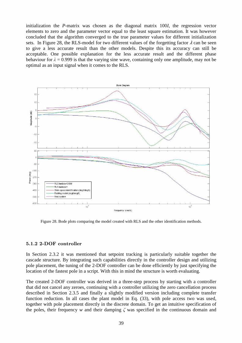
39

initialization the P-matrix was chosen as the diagonal matrix 100I, the regression vector

elements to zero and the parameter vector equal to the least square estimation. It was however

concluded that the algorithm converged to the true parameter values for different initialization

sets. In Figure 28, the RLS-model for two different values of the forgetting factor λ can be seen

to give a less accurate result than the other models. Despite this its accuracy can still be

acceptable. One possible explanation for the less accurate result and the different phase

behaviour for λ = 0.999 is that the varying sine wave, containing only one amplitude, may not be

optimal as an input signal when it comes to the RLS.

Figure 28. Bode plots comparing the model created with RLS and the other identification methods.

5.1.2 2-DOF controller

In Section 2.3.2 it was mentioned that setpoint tracking is particularly suitable together the

cascade structure. By integrating such capabilities directly in the controller design and utilizing

pole placement, the tuning of the 2-DOF controller can be done efficiently by just specifying the

location of the fastest pole in a script. With this in mind the structure is worth evaluating.

The created 2-DOF controller was derived in a three-step process by starting with a controller

that did not cancel any zeroes, continuing with a controller utilizing the zero cancellation process

described in Section 2.3.5 and finally a slightly modified version including complete transfer

function reduction. In all cases the plant model in Eq. (33), with pole access two was used,

together with pole placement directly in the discrete domain. To get an intuitive specification of

the poles, their frequency w and their damping ζ was specified in the continuous domain and

40

therefore the characteristic polynomial A0Am determining the poles was built up using an

appropriate amount of the factors

2

1 1 2A z p z p (34)

and

2 3A z p (35)

, where

0

0

1

2

1 0

2

2

3

2 cos 1s

s

s

w T

s

w T

w T

p e w T

p e

p e

(36)

The first controller was designed without model following properties or transfer function

reductions and therefore five poles were required in both the Am and A0 polynomials. This

resulted in a controller

5 4 3 2

4 3 2

5 4 3 2

0 0

3.57 3.

2.66 11.0 19.8 19.1 9.79 2.08

( 1)( 4.87 0.752)

T A 0.702 2.06 2.42 1.42 0.416 0.0488

05

z z z z z

R z z z z z

T z z z z z

S

(37)

, when using ζ = 1 and the fastest pole location possible without getting an overshoot (w0 = 20

Hz). As a result of the high order of the plant model it was necessary to place ten poles. To place

all these poles in an optimal way is not an easy task and it can therefore be a bottleneck in a

situation that requires fast tuning and high robustness. Without doing any extensive investigation

of this matter, a double pole was set at the highest frequency (w0) and then all other poles

according to 0 0 00.95 0.9 ... (1.1 0.05k)w w w on the real axis if the number of poles are

denoted by k.

The second controller version was derived using Eq. (26)-(30) with cancellation of all three plant

zeroes. With this modification, to include model following, the aim was to get a faster response

against setpoint changes. The polynomial Am was according to the minimum-phase solution

chosen to contain five poles and A0 a single pole. Equation (27) together with a monic restriction

implied the structure of R’ to be

0R z r (38)

, where r0 is a constant. As a result of the zero cancellation, the step response could be made

arbitrary fast without creating any overshoot for an ideal plant model. As seen in Figure 29, this

controller is significantly faster than the first derived controller using the values 1 and w0 =

63 Hz. To obtain an equally fast controller as the existing one it can be concluded that some

cancellation of system dynamics is required.

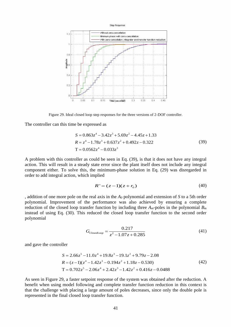
41

Figure 29. Ideal closed loop step responses for the three versions of 2-DOF controller.

The controller can this time be expressed as

4 3 2

4 3 2

4 3

0.863 3.42 5.69 4.45 1.33

1.78 0.637 0.492 0.322

T 0.0562 0.033

z z z z

R z z z z

z z

S

(39)

A problem with this controller as could be seen in Eq. (39), is that it does not have any integral

action. This will result in a steady state error since the plant itself does not include any integral

component either. To solve this, the minimum-phase solution in Eq. (29) was disregarded in

order to add integral action, which implied

0' ( 1)( )R z z r (40)

, addition of one more pole on the real axis in the A0 polynomial and extension of S to a 5th order

polynomial. Improvement of the performance was also achieved by ensuring a complete

reduction of the closed loop transfer function by including three Am-poles in the polynomial Bm

instead of using Eq. (30). This reduced the closed loop transfer function to the second order

polynomial

2

0.21

1.07 0

7

.285ClosedLoopG

z z

(41)

and gave the controller

5 4 3 2

4 3 2

5 4 3 2

2.66 11.0 19.8 19.1 9.79 2.08

( 1)( 0.194 1.18 0.530)

T 0.702 2.06 2.42 1.42 0.4

1.

16 0.

4

048

2

8

z z z z z

R z z z z z

z z

S

z z z

(42)

As seen in Figure 29, a faster setpoint response of the system was obtained after the reduction. A

benefit when using model following and complete transfer function reduction in this context is

that the challenge with placing a large amount of poles decreases, since only the double pole is

represented in the final closed loop transfer function.

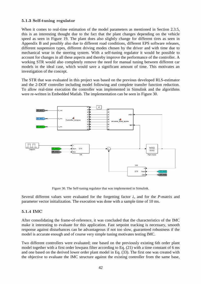
42

5.1.3 Self-tuning regulator

When it comes to real-time estimation of the model parameters as mentioned in Section 2.3.5,

this is an interesting thought due to the fact that the plant changes depending on the vehicle

speed as seen in Figure 19. The plant does also slightly change for different tires as seen in

Appendix B and possibly also due to different road conditions, different EPS software releases,

different suspension types, different driving modes chosen by the driver and with time due to

mechanical wear in the steering system. With a self-tuning regulator it would be possible to

account for changes in all these aspects and thereby improve the performance of the controller. A

working STR would also completely remove the need for manual tuning between different car

models in the ideal case, which would save a significant amount of time. This motivates an

investigation of the concept.

The STR that was evaluated in this project was based on the previous developed RLS-estimator

and the 2-DOF controller including model following and complete transfer function reduction.

To allow real-time execution the controller was implemented in Simulink and the algorithms

were re-written in Embedded Matlab. The implementation can be seen in Figure 30.

Figure 30. The Self-tuning regulator that was implemented in Simulink.

Several different values were evaluated for the forgetting factor λ, and for the P-matrix and

parameter vector initialization. The execution was done with a sample time of 10 ms.

5.1.4 IMC

After consolidating the frame-of-reference, it was concluded that the characteristics of the IMC

make it interesting to evaluate for this application. Fast setpoint tracking is necessary, smooth

response against disturbances can be advantageous if not too slow, guaranteed robustness if the

model is accurate enough and of course very simple tuning motivates testing IMC.

Two different controllers were evaluated; one based on the previously existing 6th order plant

model together with a first order lowpass filter according to Eq. (21) with a time constant of 6 ms

and one based on the derived lower order plant model in Eq. (33). The first one was created with

the objective to evaluate the IMC structure against the existing controller from the same base,

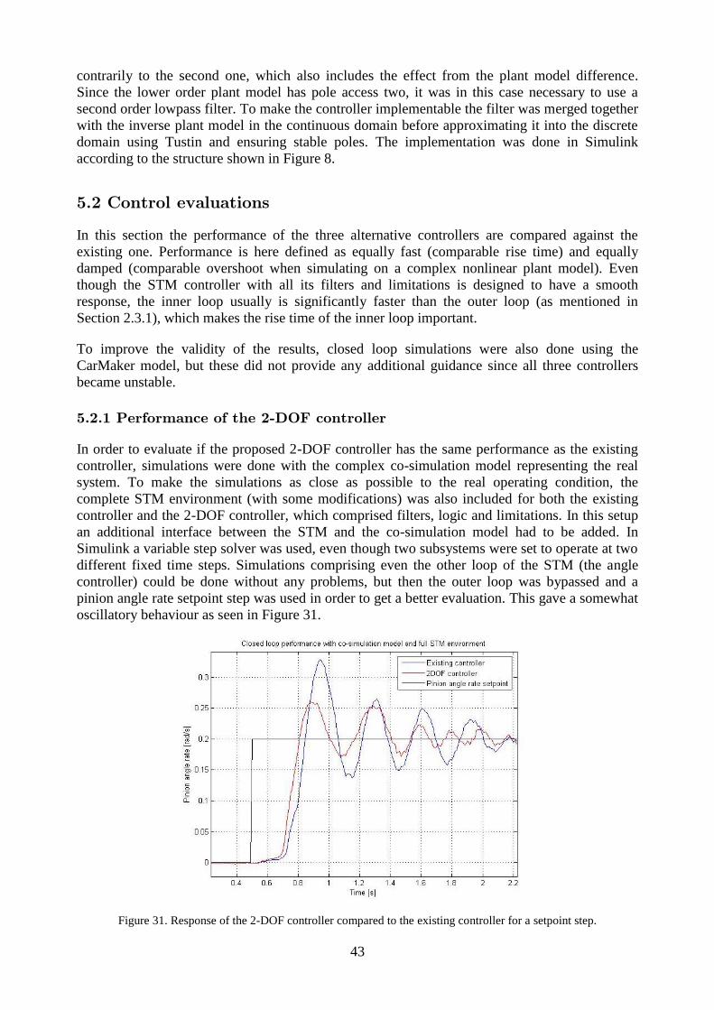
43

contrarily to the second one, which also includes the effect from the plant model difference.

Since the lower order plant model has pole access two, it was in this case necessary to use a

second order lowpass filter. To make the controller implementable the filter was merged together

with the inverse plant model in the continuous domain before approximating it into the discrete

domain using Tustin and ensuring stable poles. The implementation was done in Simulink

according to the structure shown in Figure 8.

5.2 Control evaluations

In this section the performance of the three alternative controllers are compared against the

existing one. Performance is here defined as equally fast (comparable rise time) and equally

damped (comparable overshoot when simulating on a complex nonlinear plant model). Even

though the STM controller with all its filters and limitations is designed to have a smooth

response, the inner loop usually is significantly faster than the outer loop (as mentioned in

Section 2.3.1), which makes the rise time of the inner loop important.

To improve the validity of the results, closed loop simulations were also done using the

CarMaker model, but these did not provide any additional guidance since all three controllers

became unstable.

5.2.1 Performance of the 2-DOF controller

In order to evaluate if the proposed 2-DOF controller has the same performance as the existing

controller, simulations were done with the complex co-simulation model representing the real

system. To make the simulations as close as possible to the real operating condition, the

complete STM environment (with some modifications) was also included for both the existing

controller and the 2-DOF controller, which comprised filters, logic and limitations. In this setup

an additional interface between the STM and the co-simulation model had to be added. In

Simulink a variable step solver was used, even though two subsystems were set to operate at two

different fixed time steps. Simulations comprising even the other loop of the STM (the angle

controller) could be done without any problems, but then the outer loop was bypassed and a

pinion angle rate setpoint step was used in order to get a better evaluation. This gave a somewhat

oscillatory behaviour as seen in Figure 31.

Figure 31. Response of the 2-DOF controller compared to the existing controller for a setpoint step.

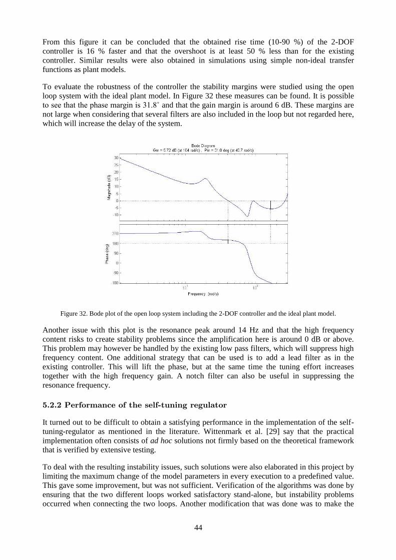
44

From this figure it can be concluded that the obtained rise time (10-90 %) of the 2-DOF

controller is 16 % faster and that the overshoot is at least 50 % less than for the existing

controller. Similar results were also obtained in simulations using simple non-ideal transfer

functions as plant models.

To evaluate the robustness of the controller the stability margins were studied using the open

loop system with the ideal plant model. In Figure 32 these measures can be found. It is possible

to see that the phase margin is 31.8˚ and that the gain margin is around 6 dB. These margins are

not large when considering that several filters are also included in the loop but not regarded here,

which will increase the delay of the system.

Figure 32. Bode plot of the open loop system including the 2-DOF controller and the ideal plant model.

Another issue with this plot is the resonance peak around 14 Hz and that the high frequency

content risks to create stability problems since the amplification here is around 0 dB or above.

This problem may however be handled by the existing low pass filters, which will suppress high

frequency content. One additional strategy that can be used is to add a lead filter as in the

existing controller. This will lift the phase, but at the same time the tuning effort increases

together with the high frequency gain. A notch filter can also be useful in suppressing the

resonance frequency.

5.2.2 Performance of the self-tuning regulator

It turned out to be difficult to obtain a satisfying performance in the implementation of the self-

tuning-regulator as mentioned in the literature. Wittenmark et al. [29] say that the practical

implementation often consists of ad hoc solutions not firmly based on the theoretical framework

that is verified by extensive testing.

To deal with the resulting instability issues, such solutions were also elaborated in this project by

limiting the maximum change of the model parameters in every execution to a predefined value.

This gave some improvement, but was not sufficient. Verification of the algorithms was done by

ensuring that the two different loops worked satisfactory stand-alone, but instability problems

occurred when connecting the two loops. Another modification that was done was to make the

45

parameter estimation loop execute in a lower frequency than the ordinary control loop. Some

improvement was obtained and as seen in Figure 33 the controller could handle the first pulse in

a pulse train before getting unstable, with the setting 0.999 and when the parameter loop

executes 10 times slower than the control loop.

Figure 33. Instability issues with the STR when the reference is a pulse train.

One property of the real plant, that does not contradict that there may be instability issues, is that

it cannot be defined as “strictly positive real”. Thereby it is not guaranteed that an adaptive

controller can be successfully implemented [7]. There is also a risk that the real-time identified

plant model has unstable poles or zeroes, which are then cancelled by the 2-DOF controller. This

is not desirable, since the identified plant model will not correspond exactly to the real system.

When the poles or zeroes are not completely cancelled the system will then become unstable. In

order to make the controller stable one possibility can be to include non-minimum phase

handling in the plant estimation as another ad hoc solution, but this still not guarantees stability.

Perhaps the system has too complex dynamical behaviour to be suitable for a STR-application.

The system behaviour may either not change enough during different operation conditions to

really motivate usage of an adaptive controller like the STR. Challenges like significantly higher

calculation load and problems with safety verification of the STR can also be very hard to

overcome. The most realistic usage of the self-tuning regulator in this context is to limit the

parameter estimations (re-tuning) to take place off-line, on behalf of a user request to tune the

controller for a new vehicle.

5.2.3 Performance of the IMC

To evaluate the IMC controller a setup with the co-simulation model, equivalent to the one

described in Section 5.2.1 was used. The result is presented in Figure 34 to the left. In this figure

the IMC controller is based on the derived transfer function in Eq. (33), but a similar result was

also obtained using the existing transfer function of the system. Even though the IMC controller

is not unstable, it can be seen that it has trouble to deal with the differences between the

simulation model and the transfer function model it is based upon. It seems like it might be more

sensitive to modelling errors than the existing controller. According to the figure, the rise time of

the IMC controller is 8.7 times longer than for the existing controller for example. The IMC

response also continues to oscillate around the steady state value even after the 2.5 s displayed in

Figure 34.

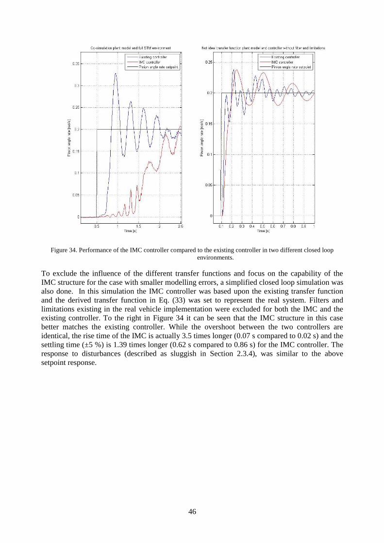
46

Figure 34. Performance of the IMC controller compared to the existing controller in two different closed loop

environments.

To exclude the influence of the different transfer functions and focus on the capability of the

IMC structure for the case with smaller modelling errors, a simplified closed loop simulation was

also done. In this simulation the IMC controller was based upon the existing transfer function

and the derived transfer function in Eq. (33) was set to represent the real system. Filters and

limitations existing in the real vehicle implementation were excluded for both the IMC and the

existing controller. To the right in Figure 34 it can be seen that the IMC structure in this case

better matches the existing controller. While the overshoot between the two controllers are

identical, the rise time of the IMC is actually 3.5 times longer (0.07 s compared to 0.02 s) and the

settling time (±5 %) is 1.39 times longer (0.62 s compared to 0.86 s) for the IMC controller. The

response to disturbances (described as sluggish in Section 2.3.4), was similar to the above

setpoint response.

47

6 DISCUSSION AND CONCLUSIONS

In this chapter a discussion about the results and some conclusions regarding the stated

research questions in Section 1.2 are presented.

6.1 Discussion

Together with the earlier presented results there has been some discussions with emphasis on

elaborating possible explanations for some results. In this section the discussion continues,

covering the most important matters regarding the final results.

6.1.1 Modelling results

The accuracy of the CarMaker model was satisfying for low frequencies up to approximately 3

Hz. By changing the inertia of the steering wheel the first resonance frequency could be matched

even better against the measurements, but no improvement of the high frequency behaviour has

been seen. The reason for this is still unknown. In section 4.2.2 the Magic Formula based tire

model and the static wheel suspension representation were mentioned as possible explanations,

but after further investigation it seems like this might not be the case. More likely the model

imperfections results from the fact that a fixed-time step solver is used to execute the Simulink

ESP-model, that the steering column representation or parameters are not accurate enough, or

that Adams performs better in simulating mechanical systems. Regarding if the model is accurate

enough to be used in the design and tuning of the STM, it can be concluded that it does not fulfil

the lowest stated frequency requirement of 8 Hz from Section 4.2.1. The closed-loop simulations

with the CarMaker model and the existing STM inner loop resulted in instability, which

furthermore justifies the conclusion that this model is not accurate enough for use in this context.

When it comes to the step responses, both models showed good correspondence for the large

step, but not equally good for the smaller step. This may depend on the models, but it can also

partly be due to that the input energy and the resulting movements are very small, which allows

disturbances and differences between the virtual and the physical test environment to influence

the results more. One identified difference is for example that the initial position of the steering

wheel was not fully centred during the physical tests, as seen in Figure 22.

The frequency behaviour of the co-simulation model showed a significant improvement

compared to the CarMaker model. Even if it was not a perfect correlation between the co-

simulation and the measurements, the model was able to reproduce all major poles and zeroes

with some fault tolerance. It is still not completely clear whether the locations of the poles and

zeroes are accurate enough for directly identifying the system inverse to be used in the STM

design. One thing that is clear though is that the model is valuable in order to give qualitative

information about how the dynamics of the system change between different vehicle models,

customer configurations and operating conditions. In other words, to enlarge the knowledge of

the system. This is valuable for decision making for example. The co-simulation model can also

be a good tool for closed-loop simulations and for evaluating the robustness of the controller.

What caused the difference between the model and the reality seems to be inaccuracy of

parameter values or of the representation of the steering wheel and steering column. The tuned

parameter values gave clearly improved amplitudes for the different frequencies, but since these

values do not originate from any measurements or similar like the default parameters do, more

investigation is needed to see whether the new values can be motivated or if the solution can be

found in any other related difference. One other possible improvement can be to exchange some

viscous damping models used against non-linear ones, providing lower damping at low velocities

48

and higher damping at high velocities. Regarding the usability of the model its complexity

results in long simulation times and sometimes in temporary simulation errors, which are time

consuming, but still manageable.

The sensitivity analysis resulted in several important conclusions for the project and showed one

possible use case of the co-simulation model. Notice however that the conclusions may only be

valid in a limited range around the used operating point. To improve the validity of these

conclusions global methods can be considered and more simulations should be done in different

speeds and with different parameter values. It is for example realistic to assume that the tires’

influence is larger for parking speeds. Synergy effects have not been studied either. The

concluded importance of the steering wheel and the steering column when it comes to the

dynamical behaviour probably originates from the fact that these components form a freely

oscillating mass. If there are hands on the steering wheel, the response and the effect from these

components will probably change significantly.

6.1.2 Control results

The final tuning of the 2-DOF controller that was used was set with the aim to provide a

critically damped, ideal closed-loop response with a rise time comparable to the one achieved

with the existing controller. This required the fastest closed-loop poles to be placed at a

frequency only ten times slower than the sampling frequency, which is on the border of what is

possible. Therefore it seems like the tuning of the existing controller is also pushed to the limit

and after comparison with other control structures its performance is still satisfying. During the

closed-loop simulations together with the co-simulation model the 2-DOF controller showed a

slightly improved performance compared to the existing controller. The overshoots of the two

controllers originate from model imperfections and in this sense the 2-DOF has shown a

tendency to be more robust against modelling errors. In this sense the structure is promising. The

limited stability margins of the open loop can however be a problem that needs further

investigation. Better stability margins have not been obtained for any of the other 2-DOF

controller versions considered in this report and not for a version based on a 2nd order plant

model either. To lift the phase it may be necessary to add additional components such as a lead

filter. Then it can be questioned how much more rapid the structure is, in terms of tuning,

compared to the existing controller even if it has the model following capabilities integrated in

the controller design. One user friendly tool that can make the tuning easier and more efficient

for both controller versions is the SISO Design Tool available in Matlab.

As concluded, the STR turned out to be hard to implement and besides the earlier comments

about this, it can once again be noted that this version of an adaptive controller seems to be not

suitable for this application. The implementation of the IMC controller was on the other hand

straight forward. It surely simplifies the controller design and thereby also the tuning, but the

closed loop simulation performance is less appealing. As mentioned in Section 2.3.4 robustness

is guaranteed, but this does not imply acceptable performance in the presence of modelling

errors, as experienced in the simulation results. Even with less modelling errors and with a less

complex simulation model, the performance of the IMC controller is not comparable to the

existing controller.

6.2 Conclusions

To make the design and tuning of a Steer-Torque-Manager more efficient through model-based

development, identified requirements on the vehicle model include:

49

To completely remove the need of a development vehicle in the design phase of the

STM, the model needs to be able to describe the system response accurately up to at least

16 Hz

If the model should be used as a plant model in closed-loop simulations, accuracy up to at

least 8 Hz is needed, but up to 16 Hz is desirable

It is advantageous if the model is maintained by the CAE Vehicle Dynamics department

It must be possible to feed the model with an EPS torque request without any inputs or

limitations on the steering wheel movement

In order to fulfil the requirements of accuracy it is crucial to involve the software

functions in the EPS, to use a variable time step solver for the Simulink EPS-model, to

have accurate friction models and to have accurate parameter values together with an

accurate representation of the torsion bar, the steering column and the steering wheel.

Neglecting the influence from the universal joints is not motivated

In order to fulfil the requirements of accuracy it is NOT crucial to use a more advanced

tire model than a Magic Formula based model (even if it is preferred), to include any

flexibility in the steering linkage between the rack and the wheels or to have particularly

high accuracy on parameters defining rack mass and vehicle roll

Regarding whether the existing inner loop of the STM-controller can be exchanged against a

similar controller allowing more rapid tuning without losing performance, one 2-DOF controller,

one STR and one IMC controller have been evaluated. To provide an equally fast response

against setpoint changes as the existing controller, some model following capabilities have been

identified as necessary. Despite the interesting theoretical capabilities of STR, it is not robust

enough to be used on this fairly complex system. Through simulations it has been shown that an

IMC controller will result in degradation of the performance. The 2-DOF controller which

includes transfer function reduction and model following has however shown slightly improved

performance compared to the existing controller. Rapid tuning in this case is also enabled

through an automated pole placement procedure. This controller thus realizes the expectations,

but before classifying it as an advantageous replacement, its robustness must be further

evaluated.

50

51

7 RECOMMENDATIONS AND FUTURE WORK

This chapter presents useful recommendations and suggestions of future work in connection to

the performed thesis subject.

7.1 Recommendations

After the completion of the project several recommendations can be given as:

Start early to acquire all the required licenses, software programs and accesses that are

needed before using any of the two evaluated vehicle models

When performing co-simulation with complex models, prevent Adams from storing the

results if the most important signals can be saved within Matlab, in order to decrease

simulation times. If the co-simulation cannot be started due to internal Matlab errors or

problems with one of the Adams s-functions, the problems usually disappear after

restarting the TCP/IP connection and Matlab and ensuring that a WiFi-connection is not

used

Be sure to gather all possible data during an experiment (for example wheel axis loads)

even if you may not think you need it, to get rid of uncertainties between the test vehicle

and the simulation model

When working with a Steer-Torque-Manager for a new vehicle model, it is of particular

importance to be observant of any differences regarding the steering wheel and the

steering column between the development vehicle and the upcoming production vehicles.

One difference can be that the airbag system is not installed in the development vehicle,

but differences may also appear through different customer adaptions or through late

design changes

7.2 Future work

In the field of the master thesis subject some future work of interest could be mentioned:

Create and evaluate a steering system model that cooperates with a simple bicycle model,

but can be executed with a variable time step solver in Simulink

Investigate how much faster and/or robust the STM controller can be made if a shorter

sampling period is possible to use

Create and evaluate a corresponding co-simulation model for the next upcoming car

model, in order to identify differences of the STM plant model before any development

vehicles are available

Gather step response and frequency data from measurements with both a different

development vehicle and a production vehicle of the same vehicle model, in order to get

a better picture of the normal distribution of the step and frequency response. This will

give more knowledge of how robust the STM has to be against modelling errors and

whether modelling results are acceptable or not

Evaluate if the accuracy of the co-simulation model can be further improved by making

the steering system structure more complex and by setting harder accuracy requirements

on the parameter values. Even more system knowledge can be obtained by measuring the

52

system response from actual applied torque to pinion movement or by performing an

eigenmode analysis in Adams for example

Identify a transfer function based on in- and output data from the co-simulation model,

implement it in the STM controller and test if its accuracy is enough by evaluating it in a

real vehicle

Evaluate if the 2-DOF controller can be made robust enough with respect to stability

margins when using the complete STM environment and test its performance in a real

vehicle

53

8 REFERENCES

[1] K. Newton, T. Garrett and W. Steeds, Motor Vehicle, Oxford: Butterworth-Heinemann,

2000, pp. 1043-1084.

[2] H. Stoll, J. Betzler and J. Reimpell, The Automotive Chassis, 2nd ed., Oxford: Elsevier

Science, 2001, pp. 86-306.

[3] TWR Inc., “Electrically Powered Steering,” [Online]. Available:

www.trw.com/steering_systems/steering/electrically_powered_steering. [Accessed 30 04

2015].

[4] L. Ljung and T. Glad, Modellbygge och simulering, vol. 2:5, Lund: Studentlitteratur AB,

2004, pp. 38-49, 249-269.

[5] J. Schoukens and R. Pintelon, System Identification: A Frequency Domain Approach,

Second ed., New Jersey: John Wiley & Sons Inc., 2012, pp. 17,18.

[6] K. Åström and T. Hägglund, PID Controllers: Theory, Design and Tuning, 2nd ed.,

Research Triangle Park, NC: Instrument Society of America, 1995, pp. 70-116, 274-297.

[7] B. Wittenmark and K. Åström, Adaptive control, 2nd ed., Upper Saddle River: Prentice

Hall, 1994, pp. 41-120.

[8] D. Katzourakis, J. de Winter, R. Happee and S. de Groot, “Driving simulator

parameterization using double-lane change steering metrics as recorded on five modern

cars,” Simulation Modelling Practice and Theory, vol. 26, no. -, pp. 96-112, 2012.

[9] J.-F. Lin, J.-H. Wu and Y.-F. Su, “Development of an interactive lane keeping control

system for vehicle,” in IEEE Vehicle Power and Propulsion Conference, Arlington, 2007.

[10] H. Mouri, K. Uenuma, M. Shimakage and S. Satoh, “Design of lane-keeping control

withsteering torque input,” JSAE Review, vol. 23, no. 3, pp. 317-323, 2002.

[11] J. Gerdes, S. Laws and Y.-H. Judy Hsu, “Estimation of Tire Slip Angle and Friction Limits

Using Steering Torque,” IEEE Transactions on Control Systems Technology, vol. 18, no.

4, pp. 896-907, 2010.

[12] R. Rajamani, Vehicle Dynamics and Control, New York: Springer Science+Business

Media, 2006, pp. 15-49.

[13] R. Granger and R. Sharp, “On car steering torques at parking speeds,” Proceedings of the

Institution of Mechanical Engineers, Part D: Journal of Automobile Engineering, vol. 217,

no. 2, pp. 87-96, 2003.

[14] B. Zhou, H. Zheng and L. Fan, “A New Control Strategy for Electric Power Steering on

Low Friction Roads,” SAE International Journal of Passenger Cars - Mechanical Systems,

vol. 7, no. 3, pp. 972-980, 2014.

[15] M. Abe, Vehicle Handling Dynamics- Theory and Application, Oxford: Elsevier's Science

& Technology, 2009, pp. 149-164.

[16] L. Ljung and T. Glad, Reglerteknik- Grundläggande teori, vol. 4:8, Lund: Studentlitteratur

AB, 2006, pp. 137-142.

54

[17] B. Lennartsson, Reglerteknikens grunder, vol. 4:6, Lund: Studentlitteratur, 2002, pp. 381-

386, 391-395.

[18] O. Arrieta, R. Vilanova and V. Alfaro, “Robust tuning of Two-Degree-of-Freedom (2-

DoF) PI/PID based cascade control systems,” Journal of Process Control, vol. 19, no. 10,

pp. 1658-1670, 2009.

[19] A. Okuyama, T. Nakamura and T. Komatsu, “Feedforward tracking control for lower-limb

robot,” in Advanced Motion Control (AMC), Yokohama, 2014.

[20] A. Visioli, “A new design for a PID plus feedforward controller,” Journal of Process

Control, vol. 14, no. 4, pp. 457-463, 2004.

[21] Q. Zou and Y. Wu, “Robust Inversion-Based 2-DOF Control Design for Output Tracking:

Piezoelectric-Actuator Example,” Control Systems Technology, IEEE, vol. 17, no. 5, pp.

1069-1082, 2009.

[22] S. Skogestad, “Simple analytic rules for model reduction and PID controller tuning,”

Journal of Process Control, vol. 13, no. 4, pp. 291-309, 2003.

[23] A. Leva, “Performance and robustness improvement in the IMC-PID Tuning Method,”

European Journal of Control, vol. 12, no. 2, pp. 195-204, 2006.

[24] I. Kaya, “Tuning PI controllers for stable processes with specifications on gain and phase

margins,” ISA Transactions, vol. 43, no. 2, pp. 297-304, 2004.

[25] I. Horn, J. Arulandu, C. Gombas, J. VanAntwerp and R. Braatz, “Improved Filter Design

in Internal Model Control,” Industrial & Engineering Chemistry Research, vol. 35, no. 10,

pp. 3437-3441, 1996.

[26] R. Vilanova, “IMC based Robust PID design: Tuning guidelines and automatic tuning,”

Journal of Process Control, vol. 18, no. 1, pp. 61-70, 2008.

[27] J. Pan, J. Yang, N. Cheung, S. Zhao and W.-C. Gan, “A Self-Tuning Regulator for the

High-Precision Control of a Linear Switched Reluctance Motor,” IEEE Transactions on

Industrial Electronics, vol. 54, no. 5, pp. 2425-2434, 2007.

[28] R. Kulhavy, “Restricted Exponential Forgetting in Real-time Identification,” Automatica,

vol. 23, no. 5, pp. 589-600, 1987.

[29] B. Wittenmark and K. Åström, “Practical Issues in the Implementation of Self-tuning

Control,” Automatica, vol. 20, no. 5, pp. 595-605, 1984.

[30] F. Mohamed and S. Yaacob, “Real time self tuning controller for induction motor based on

PI method,” in SICE Annual Conference, Morioka, 1999.

[31] MSC Software knowledge base, “Getting Started Using Adams/Controls,” 07 11 2014.

[Online]. Available:

www.simcompanion.mscsoftware.com/infocenter/index?page=content&id=DOC10042&a

ctp=LIST. [Accessed 09 04 2015].

[32] The University of Texas at El Paso, “ADAMS/Controls Version 12 TRAINING,”

[Online]. Available: www.research.utep.edu/Portals/1107/Student%20Guide.pdf.

[Accessed 22 03 2015].

[33] S. Rao, “Vehicle modeling and adams-simulink co-simulation with integrated

continuously controlled electronic suspension (ces) and electronic stability control (esc)

55

models,” Ohio State University, Columbus, 2009.

[34] T. Eriksson, “Co-Simulation of Full Vehicle Model in Adams and Anti-Lock Brake

System Model in Simulink,” Chalmers University of Technology, Göteborg, 2014.

[35] A. Schmeitz, C. Schröder, J. Pauwelussen, K.-U. Köhne, L. Gootjes and S. Jansen, “Full

vehicle ABS braking using the SWIFT rigid ring tyre model,” Control Engineering

Practice, vol. 11, no. 2, pp. 199-207, 2003.

[36] M. Gipser, “FTire, a New Fast Tire Model for Ride Comfort,” in ADAMS Users

Conference, Berlin, 1999.

[37] D. Harty and M. Blundell, The Multibody Systems Approach to Vehicle Dynamics,

Coventry: Elsevier Ltd, 2015, pp. 451-533.

[38] A. Saltelli, K. Chan and E. Scott, Sensitivity Analysis, New York: Wiley, 2008.

[39] A. Jakeman, B. Croke and J. Ticehurst, “Model design for the hydrology of tree belt

plantations on hillslopes,” Mathematics and Computers in Simulation, vol. 69, no. 1-2, pp.

188-212, 2005.

[40] D. Hamby, “A Comparison of Sensitivity Analysis Techniques,” Health Physics, vol. 68,

no. 2, pp. 195-204, 1995.

1

APPENDIX A: SELECTION OF INTERVIEW QUESTIONS

Could you describe the tuning process of the Steer-Torque-Manager today? What is the

most time consuming part of the tuning? How can it be improved? What kind of tools do

you use in this process? What would you call the method you used in tuning the inner

loop of the controller (before the final tuning in the car)?

Could you walk me through the current design of the Steer-Torque-Manager? Were some

components added afterwards, or they were added all at once? How did you conclude that

the current structure was the best to use? Did you consider any other control structure

during the design process? If you had some time left to test other control solutions, what

would you have done then, and why? Can you list the different requirements that exist on

the controller?

In previous system identification experiments, how high frequencies have you

considered? Why not any higher?

Could you describe in which context the Steer-Torque-Manager operates? Which

functions does it collaborates with? How is safety guaranteed and how does it interact

with the driver?

What components do the steering system in the new XC90 include, starting from the

steering wheel? Are there any known non-linearities, and if so, where and why? How

does the electric power steering work? Do there exist any models of its functionality?

2

APPENDIX B: TIRE COMPARISON

Figure 35. Data acquired from a previous test at Volvo Cars, performed before the start of this project. The data

illustrates the frequency behaviour from applied torque in the EPS to pinion angular velocity, for

one tire with normal profile in comparison with one low-profile tire.

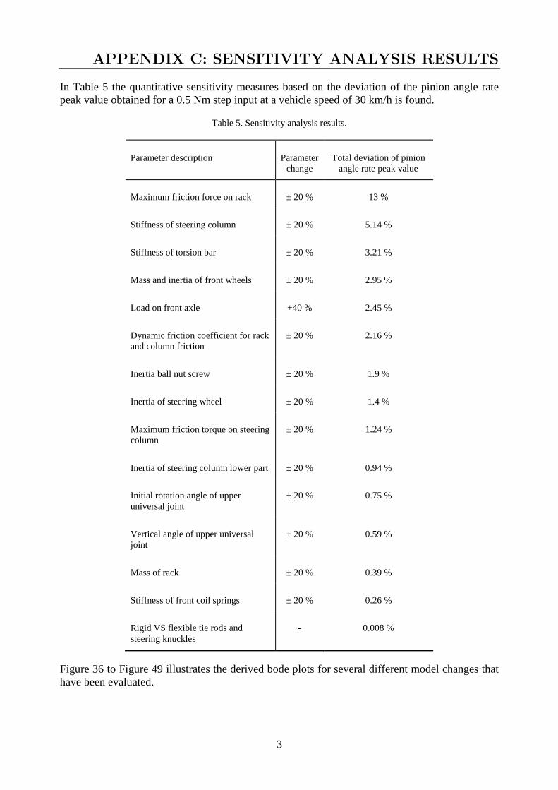
3

APPENDIX C: SENSITIVITY ANALYSIS RESULTS

In Table 5 the quantitative sensitivity measures based on the deviation of the pinion angle rate

peak value obtained for a 0.5 Nm step input at a vehicle speed of 30 km/h is found.

Table 5. Sensitivity analysis results.

Parameter description Parameter

change

Total deviation of pinion

angle rate peak value

Maximum friction force on rack ± 20 % 13 %

Stiffness of steering column ± 20 % 5.14 %

Stiffness of torsion bar ± 20 % 3.21 %

Mass and inertia of front wheels ± 20 % 2.95 %

Load on front axle +40 % 2.45 %

Dynamic friction coefficient for rack

and column friction

± 20 % 2.16 %

Inertia ball nut screw ± 20 % 1.9 %

Inertia of steering wheel ± 20 % 1.4 %

Maximum friction torque on steering

column

± 20 % 1.24 %

Inertia of steering column lower part ± 20 % 0.94 %

Initial rotation angle of upper

universal joint

± 20 % 0.75 %

Vertical angle of upper universal

joint

± 20 % 0.59 %

Mass of rack ± 20 % 0.39 %

Stiffness of front coil springs ± 20 % 0.26 %

Rigid VS flexible tie rods and

steering knuckles

- 0.008 %

Figure 36 to Figure 49 illustrates the derived bode plots for several different model changes that

have been evaluated.

4

Figure 36. Different amount of passengers.

Figure 37. Modified ball nut screw inertia.

5

Figure 38. Ten times stiffer coil springs on all four wheels.

Figure 39. Comparison between the two interfaces rack force and motor shaft torque.

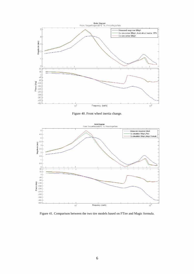
6

Figure 40. Front wheel inertia change.

Figure 41. Comparison between the two tire models based on FTire and Magic formula.

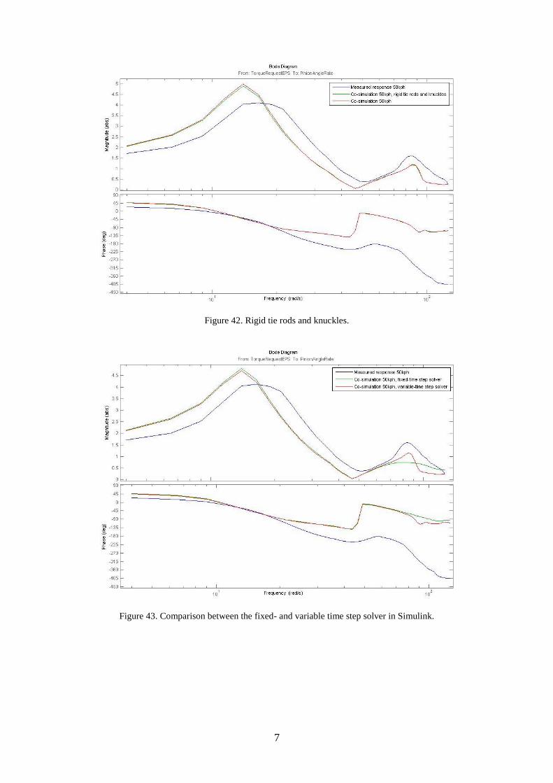
7

Figure 42. Rigid tie rods and knuckles.

Figure 43. Comparison between the fixed- and variable time step solver in Simulink.

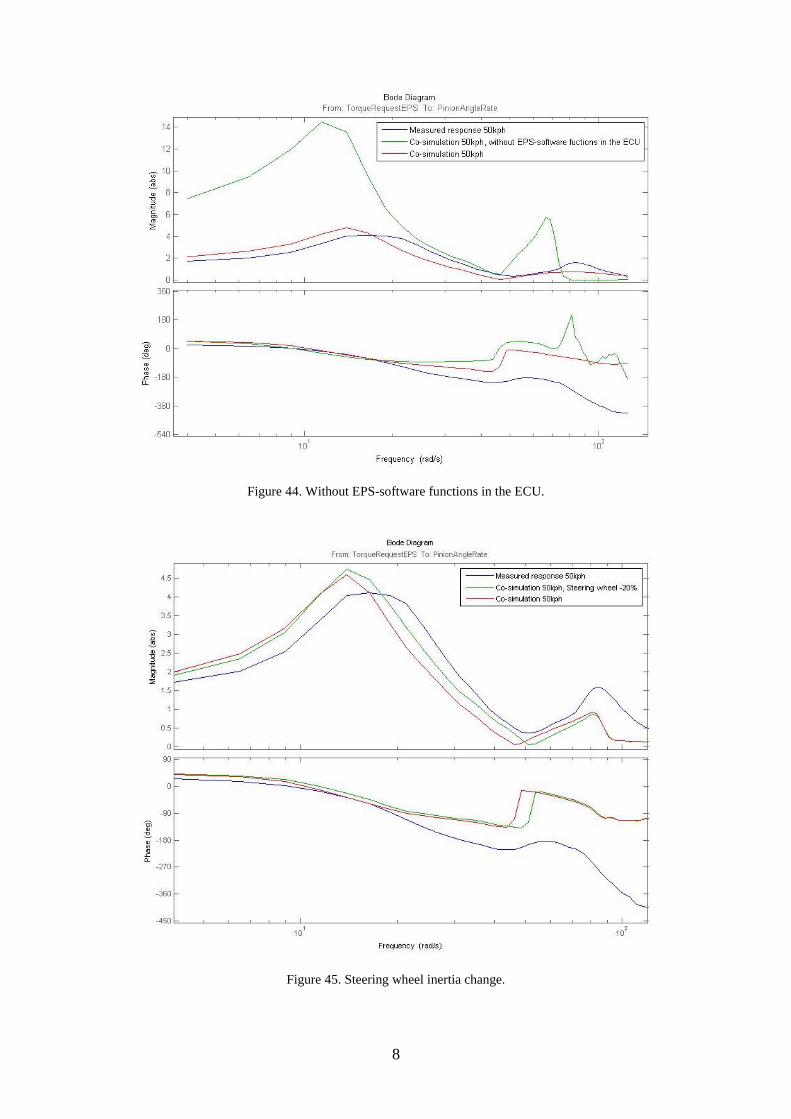
8

Figure 44. Without EPS-software functions in the ECU.

Figure 45. Steering wheel inertia change.

9

Figure 46. Torsion bar stiffness change.

Figure 47. Stiff column and torsion bar.

10

Figure 48. Straight steering column.

Figure 49. Vertical angle of upper universal joint +20 %.