reduced total energy requirements for the natario warp drive
TRANSCRIPT

Reduced Total Energy Requirements for the Natario Warp Drive
Spacetime using Heaviside Step Functions as Analytical Shape Functions.
Fernando Loup ∗
Daniel Rocha †
December 3, 2012
Abstract
Warp Drives are solutions of the Einstein Field Equations that allows superluminal travel within theframework of General Relativity. There are at the present moment two known solutions: The Alcubierrewarp drive discovered in 1994 and the Natario warp drive discovered in 2001. However as stated by bothAlcubierre and Natario themselves the warp drive violates all the known energy conditions because thestress energy momentum tensor(the right side of the Einstein Field Equations) for the Einstein tensorG00 is negative implying in a negative energy density. While from a classical point of view the negativeenergy is forbidden the Quantum Field Theory allows the existence of very small amounts of it being theCasimir effect a good example as stated by Alcubierre himself.The major drawback concerning negativeenergies for the warp drive are the huge negative energy density requirements to sustain a stable warpbubble configuration. Ford and Pfenning computed these negative energy and concluded that at least10 times the mass of the Universe is required to sustain a warp bubble configuration. However bothAlcubierre and Natario warp drives as members of the same family of the Einstein Field Equationsrequires the so-called shape functions in order to be mathematically defined. We present in this worktwo new shape functions for the Natario warp drive spacetime based on the Heaviside step function andone of these functions allows arbitrary superluminal speeds while keeping the negative energy densityat ”low” and ”affordable” levels.We do not violate any known law of quantum physics and we maintainthe original geometry of the Natario warp drive spacetime We also discuss briefly Horizons and infiniteDoppler blueshifts.
∗Residencia de Estudantes Universitas-Lisboa-Portugal-email:[email protected]†INPI- Instituto Nacional da Propriedade Industrial-Rio de Janeiro-Brazil-email:[email protected]
1

1 Introduction
The Warp Drive as a solution of the Einstein Field Equations of General Relativity that allows superlu-minal travel appeared first in 1994 due to the work of Alcubierre.([1]) The warp drive as conceived byAlcubierre worked with an expansion of the spacetime behind an object and contraction of the spacetimein front.The departure point is being moved away from the object and the destination point is being movedcloser to the object.The object do not moves at all1.It remains at the rest inside the so called warp bubblebut an external observer would see the object passing by him at superluminal speeds(pg 8 in [1])(pg 1 in [2]).
Later on in 2001 another warp drive appeared due to the work of Natario.([2]).This do not expandsor contracts spacetime but deals with the spacetime as a ”strain” tensor of Fluid Mechanics(pg 5 in [2]).Imagine the object being a fish inside an aquarium and the aquarium is floating in the surface of a river butcarried out by the river stream.The warp bubble in this case is the aquarium whose walls do not expand orcontract. An observer in the margin of the river would see the aquarium passing by him at a large speedbut inside the aquarium the fish is at the rest with respect to his local neighborhoods.
However the major drawback that affects the warp drive is the quest of large negative energy require-ments enough to sustain the warp bubble.While from a classical point of view negative energy densitiesare forbidden the Quantum Field Theory allows the existence of such energies but the major problemaffecting the Quantum Field Theory negative energies for the warp drive are the so called Quantum In-equalities(QI):The QI restricts the time we can observe a negative energy density which means to say thatas large the amount of negative energy density is then the time when this amount of energy can exists to beobserved becomes incredible small.This time is known as the sampling time which is inversely proportionalto the magnitude of the negative energy density amount.
Ford and Pfenning computed the QI for the Alcubierre warp drive using a Planck Length2 Scale shapefunction and arrived at the conclusion that the sampling time is incredible small and approximately aroundthe order of 10−33 seconds3. This means to say that the negative energy according to them can exists foronly 10−33 seconds making the warp drive an impracticable form of transport because for an interstellartrip for example a given star at 20 light years away with a warp drive speed of 200 times faster thanlight some months are required.to complete the journey but if the warp bubble can exists for only 10−33
seconds then the warp drive is impossible for such an interstellar trip. Ford and Pfenning also computedthe negative energy density requirements for the Alcubierre warp drive and they arrived at the conclusionthat in order to sustain a warp bubble able to perform interstellar travel the amount of negative energydensity is of about 10 times the mass of the universe(see pg 10 in [3])
Again they concluded that the warp drive is impossible.
However they performed all the calculations for the Alcubierre warp drive and not the Natario one.This means to say that while the Alcubierre warp drive is physically impossible the possibility or impossi-bility of Natario warp drive is still an open quest to be solved by modern science in the future.
1do not violates Relativity210−35 meters.See Wikipedia The free Encyclopedia3Consider a warp bubble with a 100 meters of radius a thickness ∆ defined by eq 23 pg 9 in [3] moving at 200 times light
speed.Look to eqs 19 pg 8 and eq 20 pg 9 in [3].Insert the thickness and the speed of the bubble in these equations and thesampling time of 10−33 seconds will appear.
2

In this work we follow the line of reason of Ford and Pfenning and we compute the total energyrequirements for the Natario warp drive.Warp drives are defined mathematically by the so-called shapefunctions.This means to say the functions that defines the mathematical structure for the geometry ofthe warp drive spacetimes.While in the Alcubierre warp drive the shape function f(rs) gives 1 in oneregion(inside the warp bubble) and 0 in another region(outside the bubble) and 1 > f(rs) > 0 in a thirdregion(warp bubble walls)(eq 7 pg 4 in [1] or top of pg 4 in [2]),in the Natario warp drive the shape functionn(rs) gives 0 in one region(inside the bubble),12 in another region(outside the bubble) and 0 < n(rs) < 1
2in a third region(warp bubble walls)(pg 5 in [2]).
We will demonstrate in this work the fact that the request or requirements of negative energy densi-ties able to sustain the geometry of the warp drive are driven by the mathematical form of the shapefunction and in a last analysis the form of the derivatives or integrals of the shape function.
However Natario point out in his work an important statement:
Any function that gives 0 in one region and 12 in another region can be regarded as a valid shape function
for the Natario warp drive spacetime.
We will demonstrate in this work that some particular choices for the shape function will produce com-pletely different mathematical results when compared between each other and some shape functions arebetter than other ones.
Ford and Pfenning arrived at the result of 10 tines the mass of the Universe for the Alcubierre warpdrive due to the particular choice they adopted for the shape function.A different shape function wouldproduce different results.And remember that their shape function was not analytical4 in all points of thetrajectory.What would happen with eq 4 pg 3 in [3] when rs = R− ∆
2 or rs = R + ∆2 ??.
All the studies about analytical shape functions for the warp drive are being carried over the Alcubierreshape function or functions constructed over the Alcubierre model.We introduce in this work the Heavisidestep functions h(rs) as valid analytical shape functions for the Natario warp drive.Dividing the Heavisidestep function that gives 0 in one region,1 in another region and 1 > h(rs) > 0 in a third region by 2 weget exactly the requested behavior of a valid Natario shape function.
In this work we introduce two Heaviside step functions as valid analytical Natario shape functions and wedemonstrate that while one of these functions still produces huge amounts of negative energy,the other keepsthe Natario warp drive with ”low” and ”affordable” amounts of negative energy even at large superluminalspeeds.
4a function in order to be analytical must be continuous and differentiable in every point of the trajectory
3

This work is divided in 4 sections:
• 1)-Basic Concepts of the Natario Warp Drive Spacetime:Warp Drive with Zero Expansion
• 2)-The Problem of the Negative Energy in the Natario Warp Drive Spacetime-The Unphysical Natureof Warp Drive
• 3)-The Heaviside Step Functions as valid Analytical Shape Functions for the Natario Warp DriveSpacetime
• 4)-Horizon and Infinite Doppler Blueshifts in both Alcubierre and Natario Warp Drive Spacetimes
The first section is a rigorous mathematical description of the basic properties of the Natario warp drivespacetime.Our goal is to produce an auto-contained or a self-contained paper with rigorous mathematicalformalism on this subject.Anyone with knowledge on differential forms can almost5 follow the study(orderive)the geometrical properties of the Natario spacetime using only 6the material presented here.
The second section illustrates the problem of the negative energy requirements in the warp drive spacetimeand why some scientists are skeptic about this concept.We compute the total energy density requirementsfor a spaceship travelling at 200 times light speed and even without Ford and Pfenning we also arrive atan unphysical result.But in the end we show that the mathematical form of the derivative of the shapefunction is very important to low or ameliorate these energy density requirements.
The third section is the most important section of this work.It presents 2 Heaviside step functions asvalid analytical shape functions for the Natario warp drive spacetime.This material is new and was nevercovered before by all the existing published or e-print literature available about warp drives7.The firstchoosen of these functions still produces a pathological result but the other produces very interesting re-sults and as a matter of fact even at 200 times light speed these functions keeps the negative energy densityat arbitrarily low levels.
The fourth section is a brief discussion of the other two problems that affects the warp drive geome-try:Horizons(causally disconnected portions of spacetime) and Doppler blueshifts outlining the fact thatthe Natario warp drive behaves slightly different when compared to its Alcubierre counterpart.
In this work the Eulerian element is defined as r2 = rs2 = [(x − xs)2 + y2 + z2] or r = rs accordingto pg 4 in [1] except in section 4.
5we outline the word almost6of course for the complex tensor calculus(e.g extrinsic curvatures etc) a computer program like the GrTensorII would be
required7as far as we can tell the Heaviside step function as an analytical shape function for the Natario warp drive never appeared
before neither in the well-known peer-review scientific publications nor in the known available e-print servers eg. arXiv,HALor viXra.We are simply confirming a fact!
4
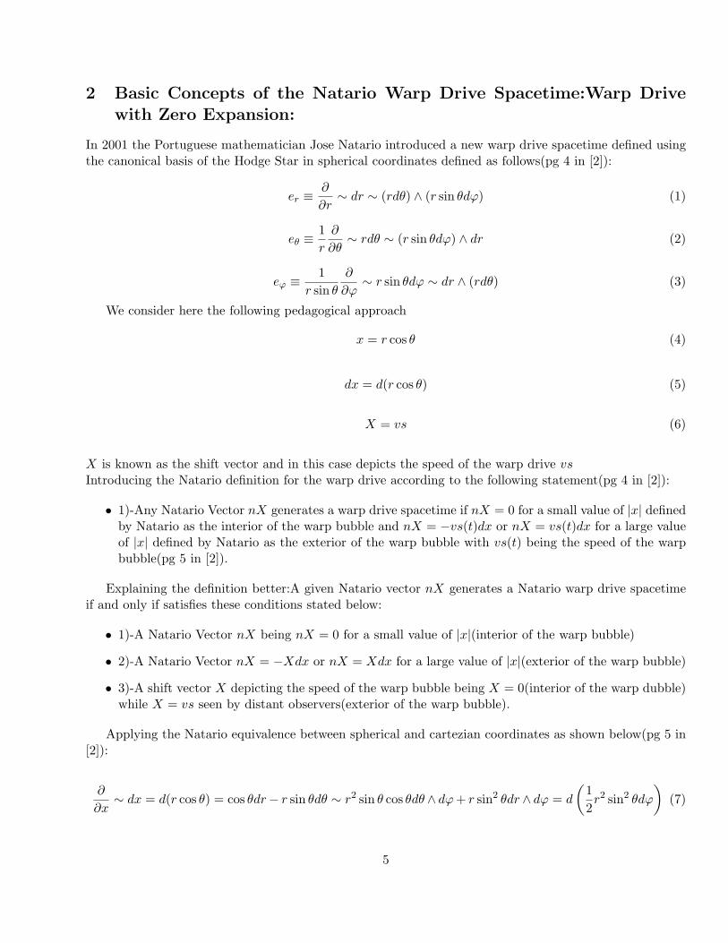
2 Basic Concepts of the Natario Warp Drive Spacetime:Warp Drivewith Zero Expansion:
In 2001 the Portuguese mathematician Jose Natario introduced a new warp drive spacetime defined usingthe canonical basis of the Hodge Star in spherical coordinates defined as follows(pg 4 in [2]):
er ≡∂
∂r∼ dr ∼ (rdθ) ∧ (r sin θdϕ) (1)
eθ ≡1r
∂
∂θ∼ rdθ ∼ (r sin θdϕ) ∧ dr (2)
eϕ ≡1
r sin θ
∂
∂ϕ∼ r sin θdϕ ∼ dr ∧ (rdθ) (3)
We consider here the following pedagogical approach
x = r cos θ (4)
dx = d(r cos θ) (5)
X = vs (6)
X is known as the shift vector and in this case depicts the speed of the warp drive vsIntroducing the Natario definition for the warp drive according to the following statement(pg 4 in [2]):
• 1)-Any Natario Vector nX generates a warp drive spacetime if nX = 0 for a small value of |x| definedby Natario as the interior of the warp bubble and nX = −vs(t)dx or nX = vs(t)dx for a large valueof |x| defined by Natario as the exterior of the warp bubble with vs(t) being the speed of the warpbubble(pg 5 in [2]).
Explaining the definition better:A given Natario vector nX generates a Natario warp drive spacetimeif and only if satisfies these conditions stated below:
• 1)-A Natario Vector nX being nX = 0 for a small value of |x|(interior of the warp bubble)
• 2)-A Natario Vector nX = −Xdx or nX = Xdx for a large value of |x|(exterior of the warp bubble)
• 3)-A shift vector X depicting the speed of the warp bubble being X = 0(interior of the warp dubble)while X = vs seen by distant observers(exterior of the warp bubble).
Applying the Natario equivalence between spherical and cartezian coordinates as shown below(pg 5 in[2]):
∂
∂x∼ dx = d(r cos θ) = cos θdr− r sin θdθ ∼ r2 sin θ cos θdθ ∧ dϕ + r sin2 θdr ∧ dϕ = d
(12r2 sin2 θdϕ
)(7)
5

We would get the following expression(pg 5 in [2])8
nX = −vs(t)d[f(r)r2 sin2 θdϕ
]∼ −2vsf(r) cos θer + vs(2f(r) + rf ′(r)) sin θeθ (8)
From now on we will use this pedagogical approach that gives results practically similar the onesdepicted in the original Natario vector shown above:
nX = −vs(t)d[f(r)r2 sin2 θdϕ
]∼ −2vsf(r) cos θdr + vs(2f(r) + rf ′(r))r sin θdθ (9)
In order to make the definition of the Natario warp drive holds true we need for the Natario vector nXa continuous Natario shape function being f(r) = 1
2 for large r(outside the warp bubble) and f(r) = 0 forsmall r(inside the warp bubble) while being 0 < f(r) < 1
2 in the walls of the warp bubble(pg 5 in [2])
To avoid confusion with the Alcubierre shape function f(rs) (pg 4 in [1])we will redefine the Natarioshape function as n(r) and the Natario vector as shown below
nX = −vs(t)d[n(r)r2 sin2 θdϕ
]∼ −2vsn(r) cos θdr + vs(2n(r) + rn′(r))r sin θdθ (10)
nX = −vs(t)d[n(r)r2 sin2 θdϕ
]∼ −2vsn(r) cos θdr + vs(2n(r) + r[
dn(r)dr
])r sin θdθ (11)
The Natario Vector nX = −vs(t)dx = 0 vanishes inside the warp bubble because inside the warpbubble there are no motion at all because dx = 0 or n(r) = 0 or X = 0 while being nX = −vs(t)dx 6= 0not vanishing outside the warp bubble because n(r) do not vanish.Then an external observer would seethe warp bubble passing by him with a speed defined by the shift vector X = −vs(t) or X = vs(t).
Redefining the Natario vector nX as being the rate-of-strain tensor of Fluid Mechanics as shown below(pg5 in [2]):
nX = Xrer + Xθeθ + Xϕeϕ (12)
Applying the extrinsic curvature for the shift vectors contained in the Natario vector nX above wewould get the following results(pg 5 in [2]):
Krr =∂Xr
∂r= −2vsn
′(r) cos θ (13)
Kθθ =1r
∂Xθ
∂θ+
Xr
r= vsn
′(r) cos θ; (14)
Kϕϕ =1
r sin θ
∂Xϕ
∂ϕ+
Xr
r+
Xθ cot θ
r= vsn
′(r) cos θ (15)
Krθ =12
[r
∂
∂r
(Xθ
r
)+
1r
∂Xr
∂θ
]= vs sin θ
(n′(r) +
r
2n′′(r)
)(16)
Krϕ =12
[r
∂
∂r
(Xϕ
r
)+
1r sin θ
∂Xr
∂ϕ
]= 0 (17)
8for a complete mathematical demonstration see Appendices B and C
6

Kθϕ =12
[sin θ
r
∂
∂θ
(Xϕ
sin θ
)+
1r sin θ
∂Xθ
∂ϕ
]= 0 (18)
Examining the first three results we can clearly see that(pg 5 in [2]):
θ = Krr + Kθθ + Kϕϕ = 0 (19)
The expansion of the normal volume elements in the Natario warp drive is Zero.
A warp drive with zero expansion.
The spacetime contraction in one direction(radial) is balanced by the spacetime expansion in the remainingdirection(perpendicular)(pg 5 in [2]).
The energy density in the Natario warp drive is given by the following expression(pg 5 in [2]):
ρ = − 116π
KijKij = − v2
s
8π
[3(n′(r))2 cos2 θ +
(n′(r) +
r
2n′′(r)
)2sin2 θ
]. (20)
ρ = − 116π
KijKij = − v2
s
8π
[3(
dn(r)dr
)2 cos2 θ +(
dn(r)dr
+r
2d2n(r)
dr2
)2
sin2 θ
]. (21)
This energy density is negative and depends on the configuration of the the Natario shape function n(r)or its derivatives..In order to generate the warp drive as a dynamical spacetime large outputs of energy areneeded due to the factor vs2 and this is a critical issue unless we use very low derivatives of the Natariowarp drive continuous shape function n(r) .
7
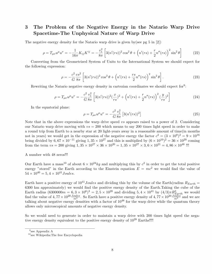
3 The Problem of the Negative Energy in the Natario Warp DriveSpacetime-The Unphysical Nature of Warp Drive
The negative energy density for the Natario warp drive is given by(see pg 5 in [2])
ρ = Tµνuµuν = − 1
16πKijK
ij = − v2s
8π
[3(n′(rs))2 cos2 θ +
(n′(rs) +
r
2n′′(rs)
)2sin2 θ
](22)
Converting from the Geometrized System of Units to the International System we should expect forthe following expression:
ρ = −c2
G
vs2
8π
[3(n′(rs))2 cos2 θ +
(n′(rs) +
rs
2n′′(rs)
)2sin2 θ
]. (23)
Rewriting the Natario negative energy density in cartezian coordinates we should expect for9:
ρ = Tµνuµuν = −c2
G
v2s
8π
[3(n′(rs))2(
x
rs)2 +
(n′(rs) +
r
2n′′(rs)
)2(
y
rs)2
](24)
In the equatorial plane:
ρ = Tµνuµuν = −c2
G
v2s
8π
[3(n′(rs))2
](25)
Note that in the above expressions the warp drive speed vs appears raised to a power of 2. Consideringour Natario warp drive moving with vs = 200 which means to say 200 times light speed in order to makea round trip from Earth to a nearby star at 20 light-years away in a reasonable amount of time(in monthsnot in years) we would get in the expression of the negative energy the factor c2 = (3 × 10⁸)2 = 9 × 10¹⁶
being divided by 6, 67× 10−11 giving 1, 35× 1027 and this is multiplied by (6× 10¹⁰)2 = 36× 1020 comingfrom the term vs = 200 giving 1, 35× 1027 × 36× 1020 = 1, 35× 1027 × 3, 6× 1021 = 4, 86× 1048 !!!
A number with 48 zeros!!!
Our Earth have a mass10 of about 6× 1024kg and multiplying this by c2 in order to get the total positiveenergy ”stored” in the Earth according to the Einstein equation E = mc2 we would find the value of54× 1040 = 5, 4× 1041Joules.
Earth have a positive energy of 1041Joules and dividing this by the volume of the Earth(radius REarth =6300 km approximately) we would find the positive energy density of the Earth.Taking the cube of theEarth radius (6300000m = 6, 3 × 10⁶)3 = 2, 5 × 10²⁰ and dividing 5, 4 × 1041 by (4/3)πR3
Earth we wouldfind the value of 4, 77×1020 Joules
m3 . So Earth have a positive energy density of 4, 77×1020 Joulesm3 and we are
talking about negative energy densities with a factor of 1048 for the warp drive while the quantum theoryallows only microscopical amounts of negative energy density.
So we would need to generate in order to maintain a warp drive with 200 times light speed the nega-tive energy density equivalent to the positive energy density of 1028 Earths!!!!
9see Appendix A10see Wikipedia:The free Encyclopedia
8
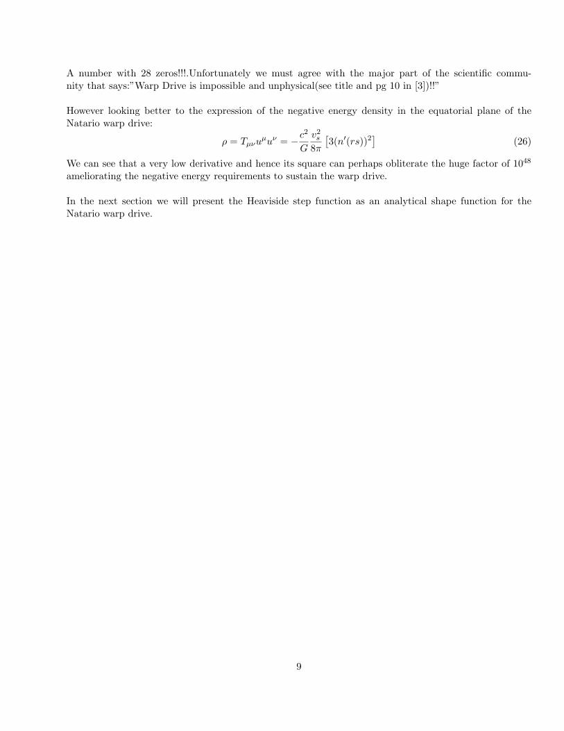
A number with 28 zeros!!!.Unfortunately we must agree with the major part of the scientific commu-nity that says:”Warp Drive is impossible and unphysical(see title and pg 10 in [3])!!”
However looking better to the expression of the negative energy density in the equatorial plane of theNatario warp drive:
ρ = Tµνuµuν = −c2
G
v2s
8π
[3(n′(rs))2
](26)
We can see that a very low derivative and hence its square can perhaps obliterate the huge factor of 1048
ameliorating the negative energy requirements to sustain the warp drive.
In the next section we will present the Heaviside step function as an analytical shape function for theNatario warp drive.
9
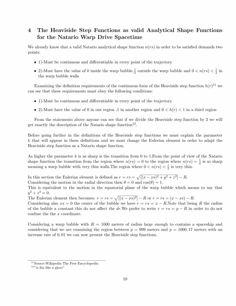
4 The Heaviside Step Functions as valid Analytical Shape Functionsfor the Natario Warp Drive Spacetime
We already know that a valid Natario analytical shape function n(rs) in order to be satisfied demands twopoints:
• 1)-Must be continuous and differentiable in every point of the trajectory
• 2)-Must have the value of 0 inside the warp bubble,12 outside the warp bubble and 0 < n(rs) < 12 in
the warp bubble walls
Examining the definition requirements of the continuous form of the Heaviside step function h(r)11 wecan see that these requirements must obey the following conditions:
• 1)-Must be continuous and differentiable in every point of the trajectory
• 2)-Must have the value of 0 in one region ,1 in another region and 0 < h(r) < 1 in a third region
From the statements above anyone can see that if we divide the Heaviside step function by 2 we willget exactly the description of the Natario shape function12.
Before going further in the definitions of the Heaviside step functions we must explain the parameterk that will appear in these definitions and we must change the Eulerian element in order to adapt theHeaviside step function as a Natario shape function.
As higher the parameter k is as sharp is the transition from 0 to 1.From the point of view of the Natarioshape function the transition from the region where n(rs) = 0 to the region where n(rs) = 1
2 is so sharpmeaning a warp bubble with very thin walls.The region where 0 < n(rs) < 1
2 is very thin.
In this section the Eulerian element is defined as r = rs =√
[(x− xs)2 + y2 + z2]−R.Considering the motion in the radial direction then θ = 0 and cos(θ) = 1.This is equivalent to the motion in the equatorial plane of the warp bubble which means to say thaty2 + z2 = 0.The Eulerian element then becomes: r = rs =
√[(x− xs)2]−R or r = rs = (x− xs)−R.
Considering also xs = 0 the center of the bubble we have r = rs = x − R.Note that being R the radiusof the bubble a constant this do not affect the dr.We prefer to write r = rs = p − R in order to do notconfuse the the x coordinate.
Considering a warp bubble with R = 1000 meters of radius large enough to contains a spaceship andconsidering that we are examining the region between p = 999 meters and p = 1000, 17 meters with anincrease rate of 0, 01 we can now present the Heaviside step functions.
11Source:Wikipedia The Free Encyclopedia12”it fits like a glove”
10

The first of these Heaviside step functions gives the value of 0 from p = 999 meters to p = 999, 99meters.At p = 1000 meters the value of 0, 5 and from p = 1000, 01 and beyond the function returns thevalue of 1 as expected by a Heaviside step function.
Remarkably the value of k being k = 10300 or k = 1050 do not affect the result.This can be confirmed byany calculation program available in any personal computer(eg. Excel,OpenOffice etc).
• 1)-The function is:
h(r) =12
+ [12] tanh(kr) (27)
• 2)-Its derivative is:
h′(r) = [12]
k
cosh(kr)2(28)
• 3)-The square of the derivative is:
h′(r)2 = [14]
k2
cosh(kr)4(29)
Integrating13 we get: ∫(h′(r)2)dr =
∫([
14]
k2
cosh(kr)4)dr (30)
∫(h′(r)2)dr = [
14][(k2)(
2 tanh(kr)3k
+tanh(kr)sech(kr)2
3k) (31)
∫(h′(r)2)dr = [
14][(k2)(
2 tanh(kr)3k
+tanh(kr)
3k cosh(kr)2) (32)
Note that we integrated in cartezian coordinates because Alcubierre wrote his metric using hyperbolicfunctions in cartezian coordinates(see eqs 6 to 8 pg 4 in [1]). Using the volume element of spherical coor-dinates which is (2π)(r2)dr the expression would be more complicated because we would need to integratehyperbolic functions in spherical coordinates but wether in cartezian or spherical coordinates both expres-sions have one thing in common.The parameter k is in the upper part of the fraction and considering that aNatario shape function would simply be the division by 2 of this step function the integration of the energydensity using this function would not ameliorate the 1048 arising from the speed 200 times faster than light.
As a matter of fact this function makes it worst due to the parameter k of (k = 10300 or k = 1050)14.13we use the on-line analytical integrator available at http://www.wolframalpha.com/14if this function do not fits our purposed then why waste time writing a lengthly expression in spherical coordinates when
want only outline the parameter k in the upper part of the fraction that appears in both expressions ??
11

The second of these Heaviside step functions gives the value of 1, 6 × 10⁻¹² from p = 999 meters top = 999, 99 meters.At p = 1000 meters the value of 0, 5 and from p = 1000, 01 and beyond the functionreturns the value of 0, 999999999... as expected by a Heaviside step function when k approaches ∞.
Like as the previous function the value of k being k = 10300 or k = 1050 do not affect the result.Thiscan be confirmed by any calculation program available in any personal computer(eg. Excel,OpenOfficeetc).Also both functions changed its values by 0, 5 exactly at 1000 meters.
We were limited by the numerical precision of Excel or OpenOffice but we have no doubts that withvalues of k even bigger we would get results even closer to 0 or even closer to 1.
• 1)-The function is:
h(r) = limk−>∞
[12
+1π
arctan(kr)] (33)
• 2)-Its derivative is:
h′(r) = limk−>∞
[1π
k
[1 + (kr)2]] (34)
• 3)-The square of the derivative is:
h′(r)2 = limk−>∞
[1π2
k2
[1 + (kr)2]2] (35)
Integrating in spherical coordinates15 we get:∫(h′(r)2)(2π)(r2))dr =
∫( limk−>∞
[1π2
k2
[1 + (kr)2]2])(2π)(r2))dr (36)
∫( limk−>∞
[1π2
k2
[1 + (kr)2]2])(2π)(r2))dr =
∫( limk−>∞
[2π
k2
[1 + (kr)2]2])(r2))dr (37)
∫( limk−>∞
[2π
k2
[1 + (kr)2]2])(r2))drs = lim
k−>∞[2π
(arctan(kr)− kr
1+(kr)2
2k)] (38)
The result above is very important:it is the core(or the nucleus) and the main reason of existence ofthis work.
Wether k being k = 10300 or k = 1050,k appears in the lower part of the fraction.Since the Natario shapefunction is the Heaviside step function divided by 2 any reader can see that this function can obliteratethe factor 1048 arising from the speed 200 times faster than light.As larger is k as lower is the energy.
15we use the on-line analytical integrator available at http://www.wolframalpha.com/
12

This was the main reason of this work:to demonstrate that the energy density requirements dependson the form of the shape function and some shape functions are better than other ones.
So a warp drive cannot be ruled out due to a pathological result if we can change the shape functionto achieve better results.
While the first Heaviside step function renders the Natario warp drive impossible,the second makes itperfectly possible
13

5 Horizon and Infinite Doppler Blueshifts in both Alcubierre and NatarioWarp Drive Spacetimes
According to pg 6 in [2] warp drives suffers from the pathology of the Horizons and according to pg 8in [2] warp drive suffer from the pathology of the infinite Doppler Blueshifts that happens when a photonsent by an Eulerian observer to the front of the warp bubble reaches the Horizon.This would render thewarp drive impossible to be physically feasible.
The Horizon occurs in both spacetimes.This means to say that the Eulerian observer cannot signal thefront of the warp bubble wether in Alcubierre or Natario warp drive because the photon sent to signal willstop in the Horizon..The solution for the Horizon problem must be postponed until the arrival of a Quan-tum Gravity theory that encompasses both General Relativity and Non-Local Quantum Entanglements ofQuantum Mechanics-
The infinite Doppler Blueshift happens in the Alcubierre warp drive but not in the Natario one.Thismeans to say that Alcubierre warp drive is physically impossible to be achieved but the Natario warp driveis perfectly physically possible to be achieved.
Consider the negative energy density distribution in the Alcubierre warp drive spacetime(see eq 8 pg6 in [3])16:
〈Tµνuµuν〉 = 〈T 00〉 =18π
G00 = − 18π
v2s(t)[y
2 + z2]4r2
s(t)
(df(rs)drs
)2
, (39)
And considering again the negative energy density in the Natario warp drive spacetime(see pg 5 in[2])17:
ρ = Tµνuµuν = − 1
16πKijK
ij = − v2s
8π
[3(n′(rs))2(
x
rs)2 +
(n′(rs) +
r
2n′′(rs)
)2(
y
rs)2
](40)
In pg 6 in [2] a warp drive with a x-axis only is considered.In this case for the Alcubierre warp drive[y2 + z2] = 0 and the negative energy density is zero but the Natario energy density is not zero and givenby:.
ρ = Tµνuµuν = − 1
16πKijK
ij = − v2s
8π
[3(n′(rs))2(
x
rs)2
](41)
The Alcubierre shape function f(rs) is defined as being 1 inside the warp bubble and 0 outside thewarp bubble while being 1 > f(rs) > 0 in the Alcubierre warped region according to eq 7 pg 4 in [1] ortop of pg 4 in [2].
Expanding the quadratic term in eq 8 pg 4 in [1] and solving eq 8 for a null-like interval ds2 = 0 wewill have the following equation for the motion of the photon sent to the front18:
dx
dt= vsf(rs)− 1 (42)
16f(rs) is the Alcubierre shape function.Equation written in the Geometrized System of Units c = G = 117n(rs) is the Natario shape function.Equation written in the Geometrized System of Units c = G = 118The coordinate frame for the Alcubierre warp drive as in [1] is the remote observer outside the ship
14

Inside the Alcubierre warp bubble f(rs) = 1 and vsf(rs) = vs.Outside the warp bubble f(rs) = 0 andvsf(rs) = 0.
Somewhere inside the Alcubierre warped region when f(rs) starts to decrease from 1 to 0 making theterm vsf(rs) decreases from vs to 0 and assuming a continuous behavior then in a given point vsf(rs) = 1and dx
dt = 0.The photon stops,A Horizon is established.This due to the fact that there are no negativeenergy density in the front of the Alcubierre warp drive in the x-axis to deflect the photon.
Now taking the components of the Natario vector defined in the top of pg 5 in [2] and inserting thesecomponents in the first equation of pg 2 in [2] and solving for the same null-like interval ds2 = 0 con-sidering only radial motion we will get the following equation for the motion of the photon sent to thefront19:
dx
dt= 2vsn(rs)− 1 (43)
The Natario shape function n(rs) is defined as being 0 inside the warp bubble and 12 outside the warp
bubble while being 0 < n(rs) < 12 in the Natario warped region according to pg 5 in [2].
Inside the Natario warp bubble n(rs) = 0 and 2vsn(rs) = 0.Outside the warpb bubble n(rs) = 12 and
2vsn(rs) = vs. Somewhere inside the Natario warped region n(rs) starts to increase from 0 to 12 making
the term 2vsn(rs) increase from 0 to vs and assuming a continuous behavior then in a given point wewould have a 2vsn(rs) = 1 and a dx
dt = 0 The photon would stops.A Horizon would be established.
However when the photon reaches the beginning of the Natario warped region it suffers a deflection by thenegative energy density in front of the Natario warp drive because this negative energy is not null.So inthe case of the Natario warp drive the photon never reaches the Horizon and the Natario warp drive neversuffer from the pathology of the infinite Doppler Blueshift due to a different distribution of energy densitywhen compared to its Alcubierre counterpart.
Adapted from the negative energy in Wikipedia:The free Encyclopedia:
”if we have a small object with equal inertial and passive gravitational masses falling in the gravitationalfield of an object with negative active gravitational mass (a small mass dropped above a negative-massplanet, say), then the acceleration of the small object is proportional to the negative active gravitationalmass creating a negative gravitational field and the small object would actually accelerate away from thenegative-mass object rather than towards it.”
19The coordinate frame for the Natario warp drive as in [2] is the ship frame observer in the center of the warp bubblexs = 0
15

6 Conclusion
In this work we demonstrated that the energy density requirements for the Natario warp drive dependson the form of the shape function.We adopted a new point of view introducing the Heaviside step functionsin the study of the Natario warp drive spacetime.This was never done before. Since one of these Heavisidestep functions allows low energy requirements and since the Natario warp drive can bypass the physicalproblem of the infinite Doppler Blueshift then the Natario warp drive can be regarded as a valid candidatefor interstellar space travel. In this work we mentioned many times our interstellar trip of 20 light years at200 times faster than light.It was inspired by the first planet discovered in the habitable zone of anotherstar:the Gliese 581 at 20 light years away.Given the huge number of planets in the habitable zones of theirparent stars example:Kepler-22 at 600 light years away or Kepler-47 at 4950 light years away these planetscan only be accessible to our space exploration if faster than light space travel could ever be developed.
16
7 Appendix A:The Natario Warp Drive Negative Energy Density inCartezian Coordinates
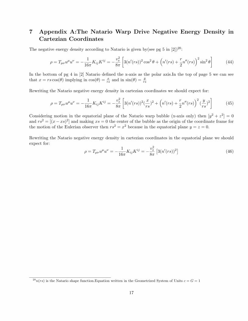
The negative energy density according to Natario is given by(see pg 5 in [2])20:
ρ = Tµνuµuν = − 1
16πKijK
ij = − v2s
8π
[3(n′(rs))2 cos2 θ +
(n′(rs) +
r
2n′′(rs)
)2sin2 θ
](44)
In the bottom of pg 4 in [2] Natario defined the x-axis as the polar axis.In the top of page 5 we can seethat x = rs cos(θ) implying in cos(θ) = x
rs and in sin(θ) = yrs
Rewriting the Natario negative energy density in cartezian coordinates we should expect for:
ρ = Tµνuµuν = − 1
16πKijK
ij = − v2s
8π
[3(n′(rs))2(
x
rs)2 +
(n′(rs) +
r
2n′′(rs)
)2(
y
rs)2
](45)
Considering motion in the equatorial plane of the Natario warp bubble (x-axis only) then [y2 + z2] = 0and rs2 = [(x− xs)2] and making xs = 0 the center of the bubble as the origin of the coordinate frame forthe motion of the Eulerian observer then rs2 = x2 because in the equatorial plane y = z = 0.
Rewriting the Natario negative energy density in cartezian coordinates in the equatorial plane we shouldexpect for:
ρ = Tµνuµuν = − 1
16πKijK
ij = − v2s
8π
[3(n′(rs))2
](46)
20n(rs) is the Natario shape function.Equation written in the Geometrized System of Units c = G = 1
17
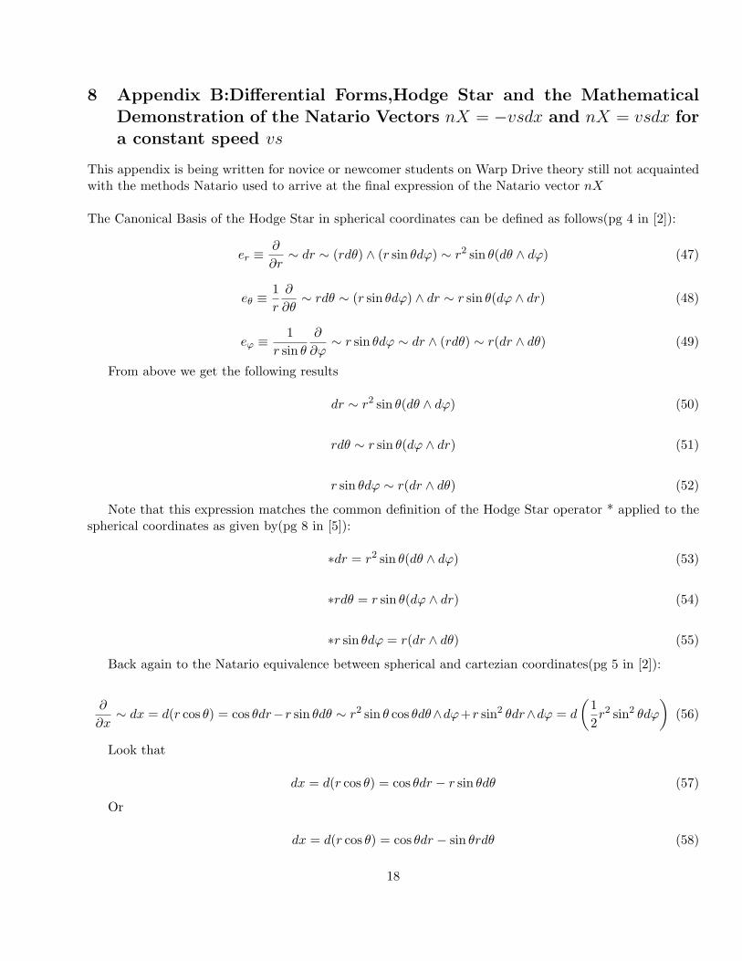
8 Appendix B:Differential Forms,Hodge Star and the MathematicalDemonstration of the Natario Vectors nX = −vsdx and nX = vsdx fora constant speed vs
This appendix is being written for novice or newcomer students on Warp Drive theory still not acquaintedwith the methods Natario used to arrive at the final expression of the Natario vector nX
The Canonical Basis of the Hodge Star in spherical coordinates can be defined as follows(pg 4 in [2]):
er ≡∂
∂r∼ dr ∼ (rdθ) ∧ (r sin θdϕ) ∼ r2 sin θ(dθ ∧ dϕ) (47)
eθ ≡1r
∂
∂θ∼ rdθ ∼ (r sin θdϕ) ∧ dr ∼ r sin θ(dϕ ∧ dr) (48)
eϕ ≡1
r sin θ
∂
∂ϕ∼ r sin θdϕ ∼ dr ∧ (rdθ) ∼ r(dr ∧ dθ) (49)
From above we get the following results
dr ∼ r2 sin θ(dθ ∧ dϕ) (50)
rdθ ∼ r sin θ(dϕ ∧ dr) (51)
r sin θdϕ ∼ r(dr ∧ dθ) (52)
Note that this expression matches the common definition of the Hodge Star operator * applied to thespherical coordinates as given by(pg 8 in [5]):
∗dr = r2 sin θ(dθ ∧ dϕ) (53)
∗rdθ = r sin θ(dϕ ∧ dr) (54)
∗r sin θdϕ = r(dr ∧ dθ) (55)
Back again to the Natario equivalence between spherical and cartezian coordinates(pg 5 in [2]):
∂
∂x∼ dx = d(r cos θ) = cos θdr−r sin θdθ ∼ r2 sin θ cos θdθ∧dϕ+r sin2 θdr∧dϕ = d
(12r2 sin2 θdϕ
)(56)
Look that
dx = d(r cos θ) = cos θdr − r sin θdθ (57)
Or
dx = d(r cos θ) = cos θdr − sin θrdθ (58)
18
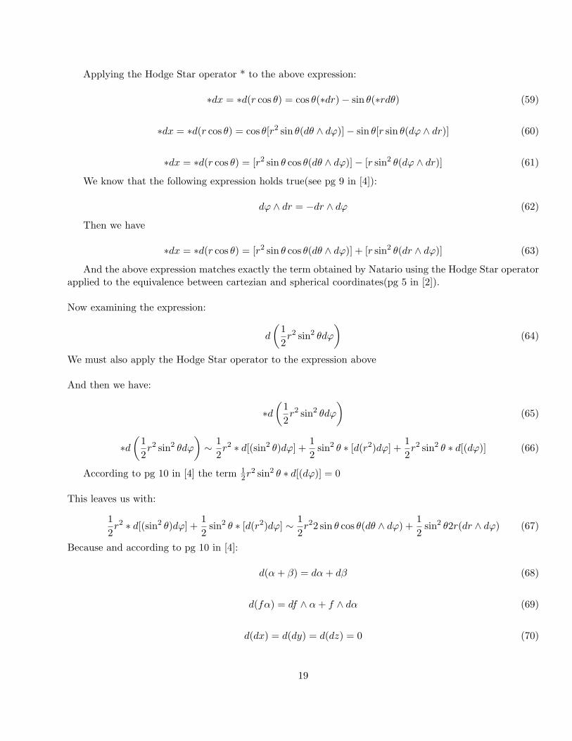
Applying the Hodge Star operator * to the above expression:
∗dx = ∗d(r cos θ) = cos θ(∗dr)− sin θ(∗rdθ) (59)
∗dx = ∗d(r cos θ) = cos θ[r2 sin θ(dθ ∧ dϕ)]− sin θ[r sin θ(dϕ ∧ dr)] (60)
∗dx = ∗d(r cos θ) = [r2 sin θ cos θ(dθ ∧ dϕ)]− [r sin2 θ(dϕ ∧ dr)] (61)
We know that the following expression holds true(see pg 9 in [4]):
dϕ ∧ dr = −dr ∧ dϕ (62)
Then we have
∗dx = ∗d(r cos θ) = [r2 sin θ cos θ(dθ ∧ dϕ)] + [r sin2 θ(dr ∧ dϕ)] (63)
And the above expression matches exactly the term obtained by Natario using the Hodge Star operatorapplied to the equivalence between cartezian and spherical coordinates(pg 5 in [2]).
Now examining the expression:
d
(12r2 sin2 θdϕ
)(64)
We must also apply the Hodge Star operator to the expression above
And then we have:
∗d(
12r2 sin2 θdϕ
)(65)
∗d(
12r2 sin2 θdϕ
)∼ 1
2r2 ∗ d[(sin2 θ)dϕ] +
12
sin2 θ ∗ [d(r2)dϕ] +12r2 sin2 θ ∗ d[(dϕ)] (66)
According to pg 10 in [4] the term 12r2 sin2 θ ∗ d[(dϕ)] = 0
This leaves us with:
12r2 ∗ d[(sin2 θ)dϕ] +
12
sin2 θ ∗ [d(r2)dϕ] ∼ 12r22 sin θ cos θ(dθ ∧ dϕ) +
12
sin2 θ2r(dr ∧ dϕ) (67)
Because and according to pg 10 in [4]:
d(α + β) = dα + dβ (68)
d(fα) = df ∧ α + f ∧ dα (69)
d(dx) = d(dy) = d(dz) = 0 (70)
19

From above we can see for example that
∗d[(sin2 θ)dϕ] = d(sin2 θ) ∧ dϕ + sin2 θ ∧ ddϕ = 2sinθ cos θ(dθ ∧ dϕ) (71)
∗[d(r2)dϕ] = 2rdr ∧ dϕ + r2 ∧ ddϕ = 2r(dr ∧ dϕ) (72)
And then we derived again the Natario result of pg 5 in [2]
r2 sin θ cos θ(dθ ∧ dϕ) + r sin2 θ(dr ∧ dϕ) (73)
Now we will examine the following expression equivalent to the one of Natario pg 5 in [2] except thatwe replaced 1
2 by the function f(r) :
∗d[f(r)r2 sin2 θdϕ] (74)
From above we can obtain the next expressions
f(r)r2 ∗ d[(sin2 θ)dϕ] + f(r) sin2 θ ∗ [d(r2)dϕ] + r2 sin2 θ ∗ d[f(r)dϕ] (75)
f(r)r22sinθ cos θ(dθ ∧ dϕ) + f(r) sin2 θ2r(dr ∧ dϕ) + r2 sin2 θf ′(r)(dr ∧ dϕ) (76)
2f(r)r2sinθ cos θ(dθ ∧ dϕ) + 2f(r)r sin2 θ(dr ∧ dϕ) + r2 sin2 θf ′(r)(dr ∧ dϕ) (77)
Comparing the above expressions with the Natario definitions of pg 4 in [2]):
er ≡∂
∂r∼ dr ∼ (rdθ) ∧ (r sin θdϕ) ∼ r2 sin θ(dθ ∧ dϕ) (78)
eθ ≡1r
∂
∂θ∼ rdθ ∼ (r sin θdϕ) ∧ dr ∼ r sin θ(dϕ ∧ dr) ∼ −r sin θ(dr ∧ dϕ) (79)
eϕ ≡1
r sin θ
∂
∂ϕ∼ r sin θdϕ ∼ dr ∧ (rdθ) ∼ r(dr ∧ dθ) (80)
We can obtain the following result:
2f(r) cosθ[r2sinθ(dθ ∧ dϕ)] + 2f(r) sinθ[r sin θ(dr ∧ dϕ)] + f ′(r)r sin θ[r sin θ(dr ∧ dϕ)] (81)
2f(r) cosθer − 2f(r) sinθeθ − rf ′(r) sin θeθ (82)
∗d[f(r)r2 sin2 θdϕ] = 2f(r) cosθer − [2f(r) + rf ′(r)] sin θeθ (83)
Defining the Natario Vector as in pg 5 in [2] with the Hodge Star operator * explicitly written :
nX = vs(t) ∗ d(f(r)r2 sin2 θdϕ
)(84)
nX = −vs(t) ∗ d(f(r)r2 sin2 θdϕ
)(85)
20
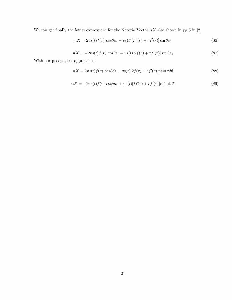
We can get finally the latest expressions for the Natario Vector nX also shown in pg 5 in [2]
nX = 2vs(t)f(r) cosθer − vs(t)[2f(r) + rf ′(r)] sin θeθ (86)
nX = −2vs(t)f(r) cosθer + vs(t)[2f(r) + rf ′(r)] sin θeθ (87)
With our pedagogical approaches
nX = 2vs(t)f(r) cosθdr − vs(t)[2f(r) + rf ′(r)]r sin θdθ (88)
nX = −2vs(t)f(r) cosθdr + vs(t)[2f(r) + rf ′(r)]r sin θdθ (89)
21
9 Appendix C:Mathematical Demonstration of the Natario Warp DriveEquation for a constant speed vs
The warp drive spacetime according to Natario is defined by the following equation but we changed themetric signature from (−,+,+,+) to (+,−,−,−)(pg 2 in [2])
ds2 = dt2 −3∑
i=1
(dxi −Xidt)2 (90)
where Xi is the so-called shift vector.This shift vector is the responsible for the warp drive behaviordefined as follows(pg 2 in [2]):
Xi = X, Y, Z y i = 1, 2, 3 (91)
The warp drive spacetime is completely generated by the Natario vector nX(pg 2 in [2])
nX = Xi ∂
∂xi= X
∂
∂x+ Y
∂
∂y+ Z
∂
∂z, (92)
Defined using the canonical basis of the Hodge Star in spherical coordinates as follows(pg 4 in [2]):
er ≡∂
∂r∼ dr ∼ (rdθ) ∧ (r sin θdϕ) (93)
eθ ≡1r
∂
∂θ∼ rdθ ∼ (r sin θdϕ) ∧ dr (94)
eϕ ≡1
r sin θ
∂
∂ϕ∼ r sin θdϕ ∼ dr ∧ (rdθ) (95)
Redefining the Natario vector nX as being the rate-of-strain tensor of fluid mechanics as shown below(pg5 in [2]):
nX = Xrer + Xθeθ + Xϕeϕ (96)
nX = Xrdr + Xθrdθ + Xϕr sin θdϕ (97)
ds2 = dt2 −3∑
i=1
(dxi −Xidt)2 (98)
Xi = r, θ, ϕ y i = 1, 2, 3 (99)
We are interested only in the coordinates r and θ according to pg 5 in [2])
ds2 = dt2 − (dr −Xrdt)2 − (rdθ −Xθdt)2 (100)
(dr −Xrdt)2 = dr2 − 2Xrdrdt + (Xr)2dt2 (101)
22
(rdθ −Xθdt)2 = r2dθ2 − 2Xθrdθdt + (Xθ)2dt2 (102)
ds2 = dt2 − (Xr)2dt2 − (Xθ)2dt2 + 2Xrdrdt + 2Xθrdθdt− dr2 − r2dθ2 (103)
ds2 = [1− (Xr)2 − (Xθ)2]dt2 + 2[Xrdr + Xθrdθ]dt− dr2 − r2dθ2 (104)
making r = rs we have the Natario warp drive equation:
ds2 = [1− (Xrs)2 − (Xθ)2]dt2 + 2[Xrsdrs + Xθrsdθ]dt− drs2 − rs2dθ2 (105)
According with the Natario definition for the warp drive using the following statement(pg 4 in [2]):anyNatario vector nX generates a warp drive spacetime if nX = 0 and X = vs = 0 for a small value of rsdefined by Natario as the interior of the warp bubble and nX = −vs(t)dx or nX = vs(t)dx with X = vsfor a large value of rs defined by Natario as the exterior of the warp bubble with vs(t) being the speed ofthe warp bubble
The expressions for Xrs and Xθ are given by:(see pg 5 in [2])
nX ∼ −2vsn(rs) cos θers + vs(2n(rs) + (rs)n′(rs)) sin θeθ (106)
nX ∼ 2vsn(rs) cos θers − vs(2n(rs) + (rs)n′(rs)) sin θeθ (107)
nX ∼ −2vsn(rs) cos θdrs + vs(2n(rs) + (rs)n′(rs)) sin θrsdθ (108)
nX ∼ 2vsn(rs) cos θdrs− vs(2n(rs) + (rs)n′(rs)) sin θrsdθ (109)
But we already know that the Natario vector nX is defined by(pg 2 in [2]):
nX = Xrsdrs + Xθrsdθ (110)
Hence we should expect for:
Xrs = −2vsn(rs) cos θ (111)
Xrs = 2vsn(rs) cos θ (112)
Xθ = vs(2n(rs) + (rs)n′(rs)) sin θ (113)
Xθ = −vs(2n(rs) + (rs)n′(rs)) sin θ (114)
23
10 Epilogue
• ”The only way of discovering the limits of the possible is to venture a little way past them into theimpossible.”-Arthur C.Clarke21
• ”The supreme task of the physicist is to arrive at those universal elementary laws from which thecosmos can be built up by pure deduction. There is no logical path to these laws; only intuition,resting on sympathetic understanding of experience, can reach them”-Albert Einstein22
11 Legacy
This work is dedicated as a tribute to memory of the English mathematician Oliver Heaviside.Althoughself-student without an university degree and ill-casted or outcasted by the great majority of the scientificcommunity of his time,his contributions prevailed and survived to our days.He adapted complex numbersto the study of electrical circuits, invented mathematical techniques to the solution of differential equations(later found to be equivalent to Laplace transforms), reformulated Maxwell’s field equations in terms ofelectric and magnetic forces and energy flux, and independently co-formulated vector analysis. Althoughat odds with the scientific establishment for most of his life, Heaviside changed the face of mathematicsand science for years to come.23 24 Without the Heaviside step function the Natario warp drive wouldperhaps remain forever as an unphysical mathematical curiosity and impossible to be achieved from a realphysical point of view.
21special thanks to Maria Matreno from Residencia de Estudantes Universitas Lisboa Portugal for providing the SecondLaw Of Arthur C.Clarke
22”Ideas And Opinions” Einstein compilation, ISBN 0− 517− 88440− 2, on page 226.”Principles of Research” ([Ideas andOpinions],pp.224-227), described as ”Address delivered in celebration of Max Planck’s sixtieth birthday (1918) before thePhysical Society in Berlin”
23quoted from Wikipedia The Free Encyclopedia24all these contributions from a man that do not have a standard university degree ranks Oliver Heaviside among the greatest
mathematicians that ever lived.And perhaps the greatest of all!!!
24
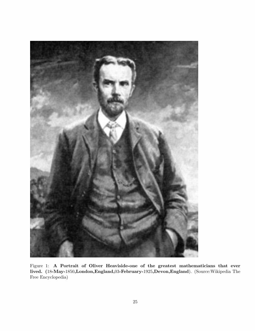
Figure 1: A Portrait of Oliver Heaviside-one of the greatest mathematicians that everlived. (18-May-1850,London,England,03-February-1925,Devon,England). (Source:Wikipedia TheFree Encyclopedia)
25
References
[1] Alcubierre M., (1994). Class.Quant.Grav. 11 L73-L77,arXiv.org@gr-qc/0009013
[2] Natario J.,(2002). Class.Quant.Grav. 19 1157-1166,arXiv.org@gr-qc/0110086
[3] Ford L.H. ,Pfenning M.J., (1997). Class.Quant.Grav. 14 1743-1751,arXiv.org@gr-qc/9702026
[4] Introduction to Differential Forms,Arapura D.,2010
[5] Teaching Electromagnetic Field Theory Using Differential Forms,Warnick K.F. Selfridge R. H.,ArnoldD. V.,IEEE Transactions On Education Vol 40 Num 1 Feb 1997
.
26