redistributive non-dissipative battery balancing …...abstract energy storage systems with many...
TRANSCRIPT
Redistributive Non-Dissipative Battery Balancing
Systems with Isolated DC/DC Converters: Theory,
Design, Control and Implementation
REDISTRIBUTIVE NON-DISSIPATIVE BATTERY BALANCING
SYSTEMS WITH ISOLATED DC/DC CONVERTERS: THEORY,
DESIGN, CONTROL AND IMPLEMENTATION
BY
LUCAS MCCURLIE, B.Tech.
a thesis
submitted to the department of electrical & computer engineering
and the school of graduate studies
of mcmaster university
in partial fulfilment of the requirements
for the degree of
Master of Applied Science
c© Copyright by Lucas McCurlie, August 2016
All Rights Reserved
Master of Applied Science (2016) McMaster University
(Electrical & Computer Engineering) Hamilton, Ontario, Canada
TITLE: Redistributive Non-Dissipative Battery Balancing Sys-
tems with Isolated DC/DC Converters: Theory, Design,
Control and Implementation
AUTHOR: Lucas McCurlie
Bachelor of Technology, Process Automation
McMaster University, Hamilton, ON, Canada
SUPERVISOR: Dr. Ali Emadi
NUMBER OF PAGES: xii, 87
ii

I would like to dedicate this thesis to my parents, John and Carmen McCurlie for
encouraging me to follow my dreams and pursue my passions. I would also like to
dedicate this to my girlfriend Stacie Wiertel for supporting me through my
academic journey and inspiring me to keep moving forward. Lastly, this thesis is
dedicated to my brother John William McCurlie. You may not be with us anymore
but the memory of you will always be in our hearts.
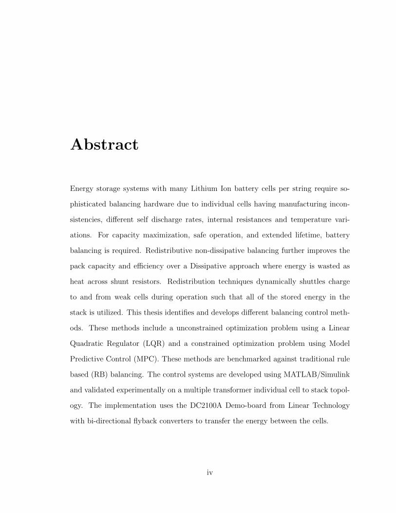
Abstract
Energy storage systems with many Lithium Ion battery cells per string require so-
phisticated balancing hardware due to individual cells having manufacturing incon-
sistencies, different self discharge rates, internal resistances and temperature vari-
ations. For capacity maximization, safe operation, and extended lifetime, battery
balancing is required. Redistributive non-dissipative balancing further improves the
pack capacity and efficiency over a Dissipative approach where energy is wasted as
heat across shunt resistors. Redistribution techniques dynamically shuttles charge
to and from weak cells during operation such that all of the stored energy in the
stack is utilized. This thesis identifies and develops different balancing control meth-
ods. These methods include a unconstrained optimization problem using a Linear
Quadratic Regulator (LQR) and a constrained optimization problem using Model
Predictive Control (MPC). These methods are benchmarked against traditional rule
based (RB) balancing. The control systems are developed using MATLAB/Simulink
and validated experimentally on a multiple transformer individual cell to stack topol-
ogy. The implementation uses the DC2100A Demo-board from Linear Technology
with bi-directional flyback converters to transfer the energy between the cells.
iv

Acknowledgements
This research was undertaken, in part, thanks to funding from the Canada Excellence
Research Chairs Program. I would like to thank my supervisor Dr. Emadi for growing
my interest and passion for Electric Vehicles. Dr. Emadi’s inspiring words fueled
my ambitions and I am truly grateful for his guidance throughout this Masters. My
deepest gratitude goes to Dr. Matthias Preindl for co-supervising this thesis research.
His teaching ability and motivation consistently challenged my boundaries and pushed
me towards my goals. I would also like to thank my friends and colleagues for all of
their support and encouragement.
v

List of abbreviations
Ah Ampere-hourBEV Battery Electric VehicleBMS Battery Management SystemC2C Cell to CellC2S Cell to StackCCS Code Composer StudioCOPM Constant Operating Point ModulationDoD Depth of DischargeEOL End of LifeEV Electric VehicleESS Energy Storage SystemHEV Hybrid Electric VehicleICE Internal Combustion EngineLi-Ion Lithium IonLQR Linear Quadratic RegulatorMPC Model Predictive ControlNiMH Nickelmetal hydrideOCV Open Circuit VoltagePHEV Plug-in Electric VehiclePWM Pulse Width ModulationRB Rule BasedS2C Stack to CellSoC State-of-ChargeSoH State-of-HealthTMS Thermal Management SystemV VoltsW WattWh Watt-hour
vi
List of symbols
C (Ah) Maximum Charge CapacityEU Total Initial Unbalanced EnergyEL Total Energy LossEA Final Additional Energy
I (A) Maximum Link Current
i (Ah) Estimated Discharge Current
i (Ah) Estimated Charge Currentic (A) Average balancing link currentIM (A) Maximum Primary Currentk High level Sampling InstantKlqr LQR GainLp (µH) Primary InductanceLs (µH) Secondary Inductancem Number of linksηB Balancing efficiencyn Number of cellsNr (2:1) Flyback Turns Ratioτ (s) Time to balanceTa (s) Maximum Operational Sampling TimeTb (s) Switch On TimeTp (s) Low level Controller Sampling TimeTs (s) High level Controller Sampling Timeu Normalized balancing currentVc (V) Cell VoltageVs (V) Stack Voltagex0 Initial State-of-chargex State-of-chargexτ Balanced State-of-charge
vii
Contents
Abstract iv
Acknowledgements v
List of abbreviations vi
List of symbols vii
1 Introduction and Problem Statement 1
1.1 Introduction . . . . . . . . . . . . . . . . . . . . . . . . . . . . . . . . 1
1.2 Research problem definition . . . . . . . . . . . . . . . . . . . . . . . 4
1.3 Research goals and requirements . . . . . . . . . . . . . . . . . . . . . 5
1.4 Electric Vehicle Battery Technologies . . . . . . . . . . . . . . . . . . 6
1.5 Basic Battery Terms . . . . . . . . . . . . . . . . . . . . . . . . . . . 11
1.6 Battery Management System (BMS) . . . . . . . . . . . . . . . . . . 14
1.7 Thesis outline . . . . . . . . . . . . . . . . . . . . . . . . . . . . . . . 15
2 Balancing methods 16
2.1 Dissipative balancing topologies . . . . . . . . . . . . . . . . . . . . . 18
2.2 Non-Dissipative balancing topologies . . . . . . . . . . . . . . . . . . 20
viii
3 Power Electronics used for Redistributive Battery Balancing 24
3.1 Overview of Power Electronics . . . . . . . . . . . . . . . . . . . . . . 24
3.2 DC-to-DC Converters . . . . . . . . . . . . . . . . . . . . . . . . . . . 25
3.2.1 Buck-boost converter . . . . . . . . . . . . . . . . . . . . . . . 25
3.2.2 Flyback converter . . . . . . . . . . . . . . . . . . . . . . . . . 29
4 Control Techniques, Analysis and Design 33
4.1 Battery System Description . . . . . . . . . . . . . . . . . . . . . . . 34
4.2 LQR Control . . . . . . . . . . . . . . . . . . . . . . . . . . . . . . . 38
4.3 MPC Control . . . . . . . . . . . . . . . . . . . . . . . . . . . . . . . 40
4.4 Rule based Control . . . . . . . . . . . . . . . . . . . . . . . . . . . . 43
5 Implementation Details 45
5.1 Linear Technology DC2100A Hardware . . . . . . . . . . . . . . . . . 45
5.2 Texas Instruments F28377D Controller . . . . . . . . . . . . . . . . . 47
5.3 Pack Harness . . . . . . . . . . . . . . . . . . . . . . . . . . . . . . . 49
5.4 Full Test Bench . . . . . . . . . . . . . . . . . . . . . . . . . . . . . . 50
5.5 Low Level Control . . . . . . . . . . . . . . . . . . . . . . . . . . . . 52
5.6 Test Procedure and Graphical User Interface . . . . . . . . . . . . . . 55
6 Simulation results and Experimental validation 58
6.1 Rule Based Control Strategy . . . . . . . . . . . . . . . . . . . . . . . 60
6.2 Linear Quadratic Regulator Control Strategy . . . . . . . . . . . . . . 61
6.3 Model Predictive Control Strategy . . . . . . . . . . . . . . . . . . . 62
6.4 Dissipative Topology for comparison . . . . . . . . . . . . . . . . . . 63
6.5 Balancing Efficiency . . . . . . . . . . . . . . . . . . . . . . . . . . . 64
ix
6.6 Discussion . . . . . . . . . . . . . . . . . . . . . . . . . . . . . . . . . 66
7 Conclusions 71
Appendix 73
A Linear Quadratic Regulator MATLAB Script . . . . . . . . . . . . . . 74
B Model Predictive Control MATLAB Script . . . . . . . . . . . . . . . 76
C Rule Based MATLAB Script . . . . . . . . . . . . . . . . . . . . . . . 78
x
List of Figures
1.1 Basic Battery Illustration [1]. . . . . . . . . . . . . . . . . . . . . . . 7
1.2 Ragone Plot of Battery Chemistries. . . . . . . . . . . . . . . . . . . 8
1.3 Trade offs Among Lithium Ion Battery Technology [2]. . . . . . . . . 9
1.4 Panasonic 18650 cell characteristics [3]. . . . . . . . . . . . . . . . . . 10
1.5 Example Balancing Strategy [4]. . . . . . . . . . . . . . . . . . . . . . 15
2.1 Passive Dissipative Balancing using Resisters. . . . . . . . . . . . . . 18
2.2 Active Dissipative Balancing using Switched Resistors. . . . . . . . . 19
2.3 Non-dissipative (Shunting) Current Divider. . . . . . . . . . . . . . . 20
2.4 Non-dissipative (Shuttling) Single Switched Capacitor. . . . . . . . . 21
2.5 Non-dissipative (Energy Converter) shared transformer. . . . . . . . . 22
2.6 Balance Hardware Topologies from [5]. . . . . . . . . . . . . . . . . . 23
2.7 Performance metrics; T2B (a), E2B (b) [5]. . . . . . . . . . . . . . . . 23
3.1 General form DC-to-DC Converter. . . . . . . . . . . . . . . . . . . . 25
3.2 Buck-Boost Converter. . . . . . . . . . . . . . . . . . . . . . . . . . . 27
3.3 Buck-Boost Converter Waveforms (CCM). . . . . . . . . . . . . . . . 28
3.4 Voltage Clamping [6]. . . . . . . . . . . . . . . . . . . . . . . . . . . . 30
3.5 Flyback Converter. . . . . . . . . . . . . . . . . . . . . . . . . . . . . 31
3.6 Flyback Converter Waveforms (DCM). . . . . . . . . . . . . . . . . . 32
xi
4.1 Multiple Transformer Balancing Topology (Flyback Converters). . . 35
5.1 DC2100A Code Communication Diagram [7]. . . . . . . . . . . . . . . 46
5.2 Oscilloscope SPI protocol with TMS320F28377D and DC2100A. . . . 48
5.3 Battery Balancing 3D Graphic of Harness. . . . . . . . . . . . . . . . 49
5.4 Battery test harness Altium PCB trace layout. . . . . . . . . . . . . . 50
5.5 Test bench. . . . . . . . . . . . . . . . . . . . . . . . . . . . . . . . . 51
5.6 LTC DC2100A simplified schematic and operational waveforms [8]. . 52
5.7 Low Level Control Switching Waveforms. . . . . . . . . . . . . . . . . 53
5.8 Measured vs. Estimated Link Currents. . . . . . . . . . . . . . . . . . 55
5.9 Programming with Matlab Coder for DSP. . . . . . . . . . . . . . . . 56
5.10 Graphical User Interface for Battery Balancing. . . . . . . . . . . . . 57
6.1 RB Simulation and Experimental Results. . . . . . . . . . . . . . . . 60
6.2 LQR Simulation and Experimental Results. . . . . . . . . . . . . . . 61
6.3 MPC Simulation and Experimental Results. . . . . . . . . . . . . . . 62
6.4 Dissipative Simulation and Experimental Results. . . . . . . . . . . . 63
6.5 RB Unbalanced(a); Balanced(b) State-of-Charge. . . . . . . . . . . . 67
6.6 LQR Unbalanced(a); Balanced(b) State-of-Charge. . . . . . . . . . . 68
6.7 MPC Unbalanced(a); Balanced(b) State-of-Charge. . . . . . . . . . . 69
xii

Chapter 1
Introduction and Problem
Statement
1.1 Introduction
Electric Vehicles (EV) have gained significant attention due to elevated atmospheric
pollution, a spreading concern for the reliance on fossil fuels as well as harsher govern-
ment policies on carbon emissions and greenhouse gases. Without any formal change
in the policy, the International Energy Agency (IEA) predicts a 70% increase in oil
consumption and a 130% increase in CO2 emissions by 2050, raising the global aver-
age temperature by 6◦C [9,10]. Despite this, the sales of alternative fuel vehicles still
suffer due to consumer range anxiety, a lack of charging stations, high initial purchase
price and longer fueling times all compared to the conventional internal combustion
engine (ICE) vehicle [11,12].
These alternative fuel vehicles include Plug-in Hybrid Electric Vehicles (PHEV),
conventional Hybrid Electric Vehicles (HEV) and full Battery Electric Vehicles (BEV).
1
M.A.Sc. Thesis - Lucas McCurlie McMaster - Electrical Engineering
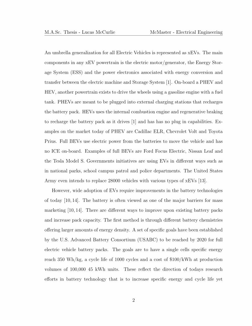
An umbrella generalization for all Electric Vehicles is represented as xEVs. The main
components in any xEV powertrain is the electric motor/generator, the Energy Stor-
age System (ESS) and the power electronics associated with energy conversion and
transfer between the electric machine and Storage System [1]. On-board a PHEV and
HEV, another powertrain exists to drive the wheels using a gasoline engine with a fuel
tank. PHEVs are meant to be plugged into external charging stations that recharges
the battery pack. HEVs uses the internal combustion engine and regenerative braking
to recharge the battery pack as it drives [1] and has has no plug in capabilities. Ex-
amples on the market today of PHEV are Cadillac ELR, Chevrolet Volt and Toyota
Prius. Full BEVs use electric power from the batteries to move the vehicle and has
no ICE on-board. Examples of full BEVs are Ford Focus Electric, Nissan Leaf and
the Tesla Model S. Governments initiatives are using EVs in different ways such as
in national parks, school campus patrol and police departments. The United States
Army even intends to replace 28000 vehicles with various types of xEVs [13].
However, wide adoption of EVs require improvements in the battery technologies
of today [10, 14]. The battery is often viewed as one of the major barriers for mass
marketing [10, 14]. There are different ways to improve upon existing battery packs
and increase pack capacity. The first method is through different battery chemistries
offering larger amounts of energy density. A set of specific goals have been established
by the U.S. Advanced Battery Consortium (USABC) to be reached by 2020 for full
electric vehicle battery packs. The goals are to have a single cells specific energy
reach 350 Wh/kg, a cycle life of 1000 cycles and a cost of $100/kWh at production
volumes of 100,000 45 kWh units. These reflect the direction of todays research
efforts in battery technology that is to increase specific energy and cycle life yet
2
M.A.Sc. Thesis - Lucas McCurlie McMaster - Electrical Engineering
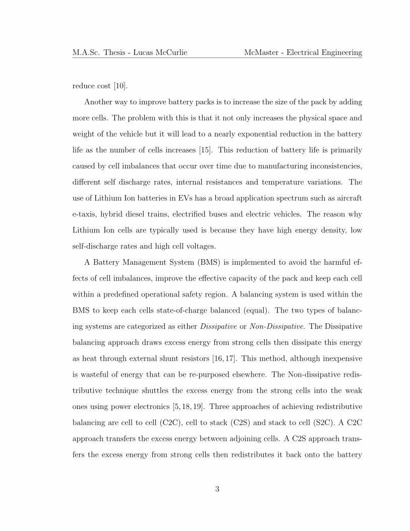
reduce cost [10].
Another way to improve battery packs is to increase the size of the pack by adding
more cells. The problem with this is that it not only increases the physical space and
weight of the vehicle but it will lead to a nearly exponential reduction in the battery
life as the number of cells increases [15]. This reduction of battery life is primarily
caused by cell imbalances that occur over time due to manufacturing inconsistencies,
different self discharge rates, internal resistances and temperature variations. The
use of Lithium Ion batteries in EVs has a broad application spectrum such as aircraft
e-taxis, hybrid diesel trains, electrified buses and electric vehicles. The reason why
Lithium Ion cells are typically used is because they have high energy density, low
self-discharge rates and high cell voltages.
A Battery Management System (BMS) is implemented to avoid the harmful ef-
fects of cell imbalances, improve the effective capacity of the pack and keep each cell
within a predefined operational safety region. A balancing system is used within the
BMS to keep each cells state-of-charge balanced (equal). The two types of balanc-
ing systems are categorized as either Dissipative or Non-Dissipative. The Dissipative
balancing approach draws excess energy from strong cells then dissipate this energy
as heat through external shunt resistors [16, 17]. This method, although inexpensive
is wasteful of energy that can be re-purposed elsewhere. The Non-dissipative redis-
tributive technique shuttles the excess energy from the strong cells into the weak
ones using power electronics [5, 18, 19]. Three approaches of achieving redistributive
balancing are cell to cell (C2C), cell to stack (C2S) and stack to cell (S2C). A C2C
approach transfers the excess energy between adjoining cells. A C2S approach trans-
fers the excess energy from strong cells then redistributes it back onto the battery
3
M.A.Sc. Thesis - Lucas McCurlie McMaster - Electrical Engineering
stack. Likewise, a S2C approach transfers the excess energy from the battery stack
to the weak cells. It is possible to achieve simultaneously charge and discharge of
individual cells by integrating a S2C with C2S.
Each method can use different types of strategies to control the battery currents
for individual cells. In this thesis, a redistributive non-dissipative battery balancing
system is developed using flyback converters for shuttling the energy simultaneous
to and from each cell in the pack. Different control strategies are implemented on
top of the hardware to compare performance variation and to help understand better
balancing practices. Furthermore, a model predictive control technique is developed
using performance metrics from [5], which balances the cells in minimum time. A
minimum time to balance control can be used in electric fleet vehicles where time
to balance is important. Other applications for redistributive control are further
explored.
1.2 Research problem definition
Electric fleet vehicles are becoming more common as companies are starting to real-
ize the advantage of lower operating and maintenance costs [13]. Medium and heavy
duty Battery Electric Vehicles and Plug-In Hybrids have begun penetrating several
transportation sectors such as transit buses and delivery vehicles. Benefits in these
sectors are reduced road traffic noise, less noise polluted cities and more sustainable
transportation. Further improvements over ICEs are due to a reduction in mainte-
nance cost (as brakes do not wear as easily due to regenerative braking), fewer engine
fluids and fewer moving parts [20]. By 2020, Fort Motor Company believes that 10%
to 25% of its global fleet will be electrified. Purolator is purchasing more electric
4

M.A.Sc. Thesis - Lucas McCurlie McMaster - Electrical Engineering
vehicles for delivery application; Ford and Frieghtliner will be selling full BEV utility
vehicles soon and Navistar intends to produce EVs as well [13].
Lithium Ion batteries require balancing due to individual cells having manufactur-
ing inconsistencies, different self discharge rates, internal resistances and temperature
variations. The desired result of this research is to present a Non-dissipative redis-
tributive balancing system to further improve on the pack capacity and balancing
efficiency over a active dissipative approach being deployed in most EVs. As batter-
ies are charged and discharges in a vehicle, they degrade over time. Car manufactures
typically define the end-of-life (EOL) as 20% reduction in the battery capacity from
when it was first installed into the car. This degradation also increases the resistance
and reduces the amount of power the battery is able to deliver. However, once a cell
reaches this 20% reduction in battery capacity does not mean it cannot be used for
another purpose.
Two applications where redistributive non-dissipative balancing may be useful in
the future are in delivery fleet vehicles and second life battery applications. Delivery
fleet vehicles might find it useful to have a minimum time to balance implementation
since this could mean more time on the road. Battery second life applications use
recycled battery packs for stationary power systems with mismatched capacities and
large initial imbalances. Having optimization methods embedded in the balancing,
could mean weak capacity cells would not hinder the system.
1.3 Research goals and requirements
Different control approaches are simulated using Matlab Simulink and are compared
to experimental results conducted on a small test bench lab setup. The three control
5
M.A.Sc. Thesis - Lucas McCurlie McMaster - Electrical Engineering
approaches being compared are Rule Based (RB), Linear Quadratic Regulator (LQR)
and Model Predictive Control (MPC). Results show that MPC and LQR achieve a
single point convergence of the state-of-charge when compared against a common
Rule Based algorithm. However, LQR balances in less time due to saturation of the
balancing currents. RB and MPC balance in the same time but MPC has a higher
balancing efficiency.
In this thesis, a new performance metric is introduced for battery balancing. The
balancing hardware and control strategy have a associated balancing efficiency (ηB).
This balancing efficiency is attributed to the total amount of initial unbalanced energy
and the total amount of lost energy during balancing the cells. This metric is used to
compare RB control and the MPC as both provide nearly optimal minimum time to
balance but MPC has higher balancing efficient. It is also used to show that active
dissipative approach has a balancing efficiency of zero due to all the unbalanced energy
being lost as heat to the resistors.
1.4 Electric Vehicle Battery Technologies
A battery contains a number of electrically connected cells that convert stored chem-
ical energy into electric energy. Each cell is a combination of two electrodes arranged
so that an overall oxidation-reduction reaction produces an electromotive force. There
exists several types of batteries, all with different applications. A primary battery is
one that is disposable and cannot be recharged. It has irreversible chemical reactions
inside the electrode to generate electricity. In the attempt to recharge this type of
battery, it would produce hazardous liquids that would eventually leak. For an ex-
ample, a Alkaline Manganese cell known as the common household battery is often
6
M.A.Sc. Thesis - Lucas McCurlie McMaster - Electrical Engineering
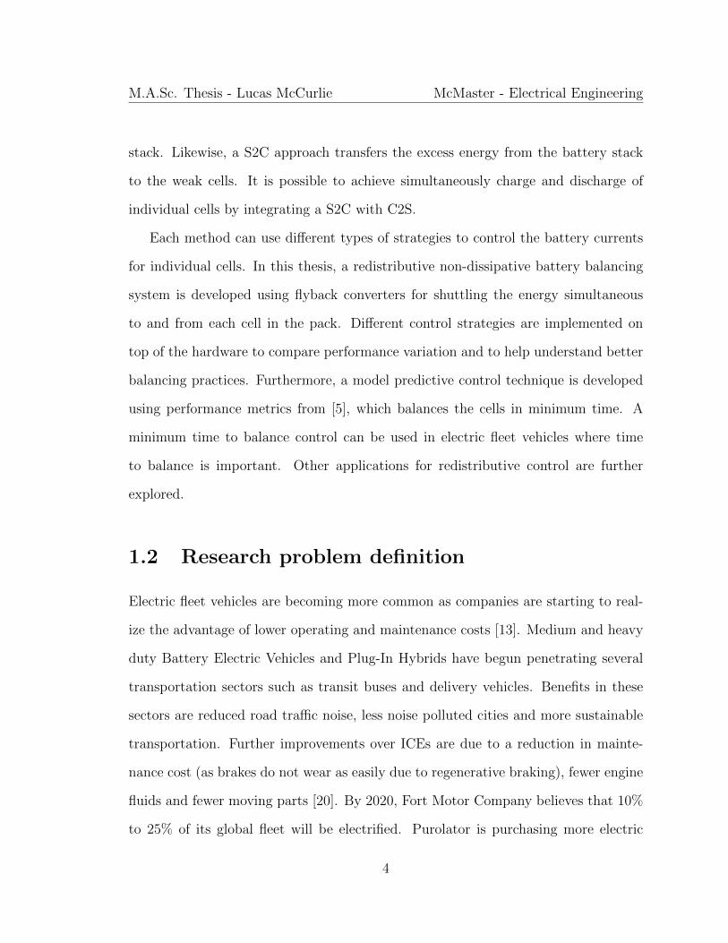
Figure 1.1: Basic Battery Illustration [1].
found in smoke alarms and Television remotes.
A secondary battery is one that involves a reversible chemical reaction and can
be recharged multiple times. This type of battery is used in Electric Vehicles for
obvious reasons but can also be found in ICEs as Lead-acid batteries for starting the
car. The components of a secondary battery consist of a anode, cathode, separators,
current collector and electrolyte. The anode is the negative electrode and is where
the electrons are generated. The cathode is the positive electrode and is where the
electrons return after doing work outside of the battery. The separator is the insulat-
ing divider and is physically separated by the two electrodes. It helps move the ions
from one electrode to the other and also prevents any electrons from crossing over.
The current collector is placed on each of the electrodes and its primary function is to
conduct electrons to and from the external electrical circuit. The final component is
the electrolyte. This facilitates ions that are essential to support the electrochemical
reactions.
Due to its superior performance, Lithium ion batteries are leading the EV market
over Lead acid batteries and NiMH batteries [10, 21, 22]. For this reason, it will be
used as the main focus for this thesis. The anode (negative electrode) is made of
carbon and the cathode (positive electrode) consists of a metal oxide. The charging
7
M.A.Sc. Thesis - Lucas McCurlie McMaster - Electrical Engineering
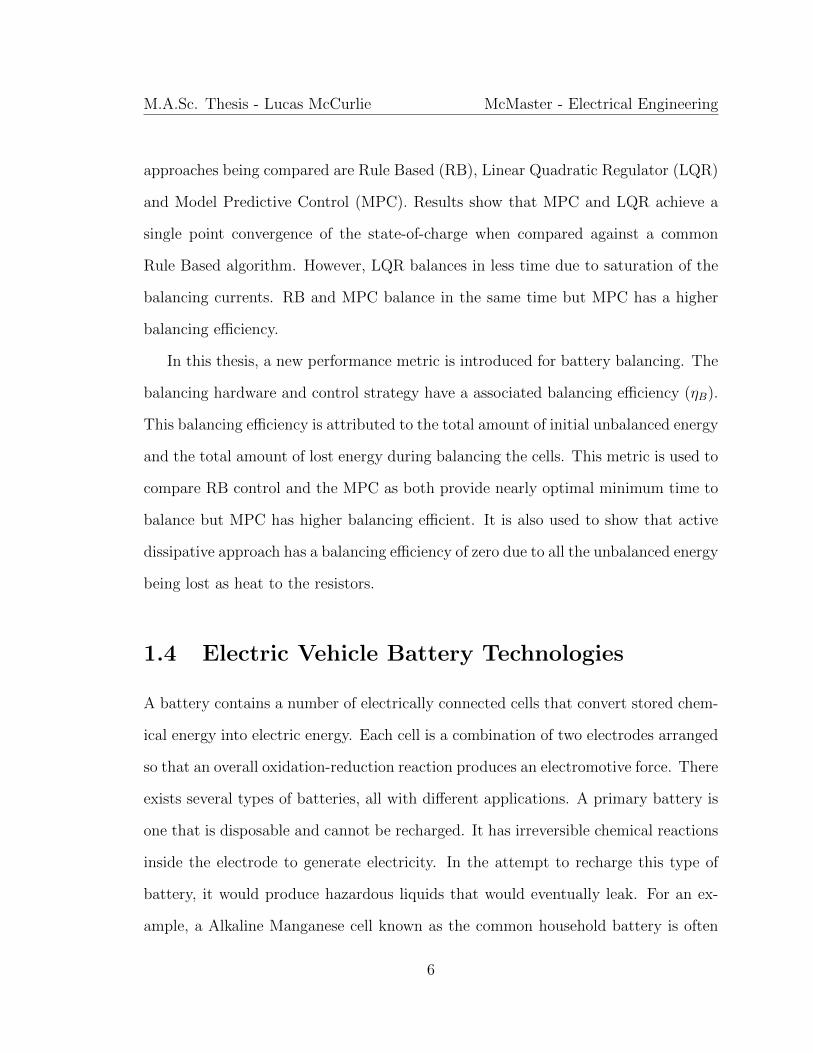
Figure 1.2: Ragone Plot of Battery Chemistries.
and discharging of the cell occurs by transferring Lithium ions between these two
electrodes across the solution and electrons through the current collectors. The sep-
arator will inhibit the flow of electrons but conduct ions. Fig. 1.1 shows different cell
formats such (a) small cylindrical cell, (b) prismatic cell and (c) pouch cell. Each
format has an appropriate application and is up to the engineer to decide what works
best. A more detailed comparison between the different formats can be found in [4].
Lithium Ion batteries typically have a flat discharge curve that associates cell
capacity (Ah) to the cells open circuit voltage (OCV). Different curves for different
c-rates are provided by many battery manufacturing companies and can be shown
in Fig. 1.4. The advantage of having a flat discharge curve is that it simplifies the
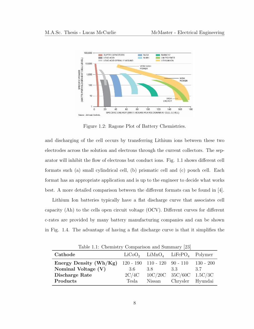
Table 1.1: Chemistry Comparison and Summary [23]
Cathode LiCoO2 LiMnO4 LiFePO4 Polymer
Energy Density (Wh/Kg) 120 - 190 110 - 120 90 - 110 130 - 200Nominal Voltage (V) 3.6 3.8 3.3 3.7Discharge Rate 2C/4C 10C/20C 35C/60C 1.5C/3CProducts Tesla Nissan Chrysler Hyundai
8
M.A.Sc. Thesis - Lucas McCurlie McMaster - Electrical Engineering
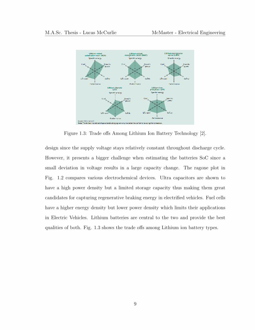
Figure 1.3: Trade offs Among Lithium Ion Battery Technology [2].
design since the supply voltage stays relatively constant throughout discharge cycle.
However, it presents a bigger challenge when estimating the batteries SoC since a
small deviation in voltage results in a large capacity change. The ragone plot in
Fig. 1.2 compares various electrochemical devices. Ultra capacitors are shown to
have a high power density but a limited storage capacity thus making them great
candidates for capturing regenerative braking energy in electrified vehicles. Fuel cells
have a higher energy density but lower power density which limits their applications
in Electric Vehicles. Lithium batteries are central to the two and provide the best
qualities of both. Fig. 1.3 shows the trade offs among Lithium ion battery types.
9

M.A.Sc. Thesis - Lucas McCurlie McMaster - Electrical Engineering
Fig
ure
1.4:
Pan
ason
ic18
650
cell
char
acte
rist
ics
[3].
10

M.A.Sc. Thesis - Lucas McCurlie McMaster - Electrical Engineering
1.5 Basic Battery Terms
In order to fully describe the state and properties of different battery cells, commonly
used terms are summarized in the following as a quick reference.
Cell, module, pack. A single cell has two electrodes, separator and electrolyte.
A module is a few cells in series or parallel with one another. The battery pack is
comprised of many modules to accommodate high voltages and large capacities. For
example, the Chevrolet Volt uses 96 Lithium Ion cells in its pack construction.
State-of-Charge (SoC). SoC is an expression that indicates the amount of battery
capacity as a percentage of the maximum capacity. The state of charge x is not
measurable but can be estimated according to y = C(x) where y is the voltage asso-
ciated with the battery terminals and C is some nonlinear mapping [24]. Advanced
methods for SoC estimation are Kalman filters [25], neural networks [26], electro-
chemical impedance spectroscopy [27] and fuzzy logic [28,29]. If Ah capacity is used,
the change of SoC can be expressed as
∆SoC = SoC(t)− SoC(t0) =1
Ah Capacity
∫ t
t0
u(t)dt (1.1)
State-of-Health (SoH). SoH is a ratio of the maximum charge capacity of an aged bat-
tery to the maximum charge capacity when the battery was new. It can be expressed
as
SoH =Aged Energy Capacity
Nomincal Energy Capacity(1.2)
11

M.A.Sc. Thesis - Lucas McCurlie McMaster - Electrical Engineering
Terminal Cell voltage (V). Terminal voltage (Vt) is measured between the battery
terminals with a load being applied. This changes with state-of-charge and applied
current.
Open circuit voltage (V). The voltage that is measured between the battery ter-
minals when no load is applied.
Capacity (Ah). The capacity of a battery is the amount of current it can provide
for a certain amount of time. It is typically expressed in Amphours. For example,
the Panasonic 18650 cells shown in Fig. 1.4 has a nominal capacity of 3.07 Ah.
C-rate. Typically used when describing how much current a type of battery cell
can discharge. A C-rate is a measure of the rate at which a battery can discharge
relative to its maximum capacity. A 1C rate means that the discharge current will
discharge the entire battery in 1 hour. For a battery with a capacity of 50 Amphours,
this equates to a discharge current of 50 Amps. A 5C rate for this battery would be
250 Amps, and a C/2 rate would be 25 Amps.
Cycle Life. Cycle life is the number of discharge-charge cycles before a battery
fails to meet specific performance criteria. Under specific charge and discharge con-
ditions, Cycle life can be estimated. The operating life is affected by the rate and
depth of cycles as well as temperature and humidity.
12
M.A.Sc. Thesis - Lucas McCurlie McMaster - Electrical Engineering
Internal resistance. Internal Resistance is the resistance within the battery. In
general, it is dependent on the cells state-of-charge and if its being charged or dis-
charged. The batteries efficiency decreases as the internal resistance increases.
Depth of Discharge (DoD). The percentage of battery capacity that has been
discharged expressed as a percentage of maximum capacity.
DoD = 1− SoC (1.3)
Stored Energy (Wh). The energy stored in a battery depends on its voltage and
capacity. A unit of Watthour is typically used.
Stored energy (Wh) = Voltage (V) x Capacity (Ah) (1.4)
Specific energy. Specific energy is the quantity of energy stored in the battery for
every kilogram of mass. The specific energy is typically given in Wh/Kg.
Specific Energy =Stored Energy (Wh)
Battery Mass (Kg)(1.5)
Specific power. Specific power is the amount of power obtained for each kilogram
of the battery and is measured in W/Kg.
Specific Power =Peak Power (W)
Battery Mass (Kg)(1.6)
Thermal management System. TMS protects the battery pack from overheating.
This can help extend the packs calender life. EVs which use NiMH batteries use
13
M.A.Sc. Thesis - Lucas McCurlie McMaster - Electrical Engineering
simple forced air cooling TMS, but more sophisticated and powerful liquid cooling is
required for Lithium ion batteries in EV Applications [30].
1.6 Battery Management System (BMS)
The Battery Management System (BMS) is a system used for the following tasks:
1. Monitoring
2. Protection
3. Estimation
4. Control
These four main functions are found in any BMS to ensure safe operation, high
performance and longer lifetime expectancy [31, 32]. Protection of Lithium-ion bat-
teries experiencing over and under voltages is essential to maximizing the health and
safety of the cells [33]. If over voltage occurs, production of CO2, C2H4 and other
gases will increase the internal temperature and pressure causing severe battery dam-
age or an explosion [32]. If under voltage occurs, internal reactions cause the cell to
lose a large part of its capacity. The voltage of a battery cell is related to its remain-
ing energy (state-of-charge). Therefore, a weak cell is defined as one that has a lower
SoC than the others in the pack. Likewise a strong cell is one that has a higher SoC.
Without a on-board balancing system, the cells capacities would drift apart causing
weak cells to dominate discharging time and strong cells to dominate charging time.
A Battery Management System (BMS) is implemented to avoid the harmful effects of
cell imbalances, improve the effective capacity of the pack and keep each cell within
14
M.A.Sc. Thesis - Lucas McCurlie McMaster - Electrical Engineering
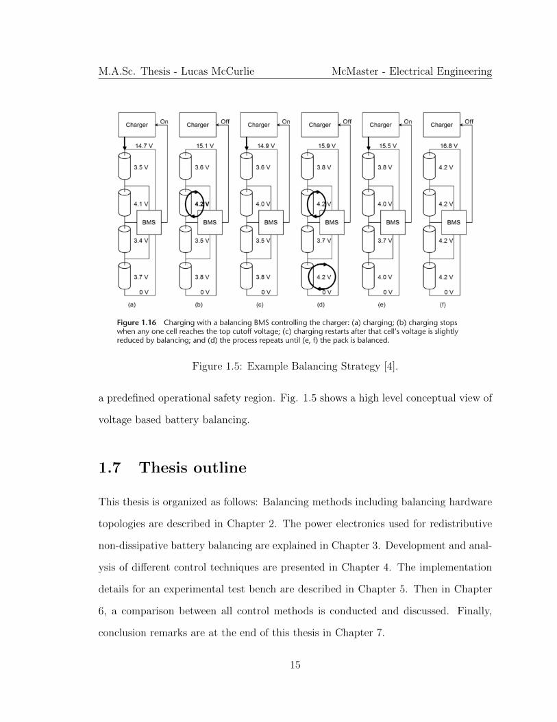
Figure 1.5: Example Balancing Strategy [4].
a predefined operational safety region. Fig. 1.5 shows a high level conceptual view of
voltage based battery balancing.
1.7 Thesis outline
This thesis is organized as follows: Balancing methods including balancing hardware
topologies are described in Chapter 2. The power electronics used for redistributive
non-dissipative battery balancing are explained in Chapter 3. Development and anal-
ysis of different control techniques are presented in Chapter 4. The implementation
details for an experimental test bench are described in Chapter 5. Then in Chapter
6, a comparison between all control methods is conducted and discussed. Finally,
conclusion remarks are at the end of this thesis in Chapter 7.
15
Chapter 2
Balancing methods
Electric Vehicles are rapidly shifting towards drivetrains with high-power electric
machines and inverters. The battery system therefore needs to be high voltage, high
efficiency and have long lifetime [22,34–36]. The battery cells are connected in series
to achieve high voltage levels which will lead to a nearly exponential reduction in
the battery life as the number of cells increases [15]. A significant reason for reduced
lifetime is charge imbalances of the cells which only degrades even further with time.
Cell imbalances arise due to internal effects such as manufacturing inconsistencies,
different self-discharge rates and internal resistance as well as external effects such as
temperature variations. To avoid damages, correct any imbalances and improve the
effective capacity of the pack, an energy balancing system is required [37].
The two types of battery balancing hardware is dissipative and non-dissipative.
A dissipative approach draws excess charge from the cells with a higher state-of-
charge and dissipates it through resistors. A non-dissipative approach uses power
electronics to transfer excess charge between cells [5, 18, 19, 38]. Balancing simply
means equalizing all cells state-of-charge in a series connected string. If a unbalanced
16

M.A.Sc. Thesis - Lucas McCurlie McMaster - Electrical Engineering
string remains as such, the effective capacity of the pack is low. As mentioned before,
Lithium Ion battery cells are typically used in EVs because of their superior energy
density, self discharge rate and cycle life. However, Li-ion cells have more safety
precautions than lead-acid and NiMH [4]. This means while discharging the stack,
operation must halt once the weakest cell is completely empty, even if the stronger
cells still contain energy. Redistribution is defined as dynamically shuttling charge
to the weak cells from the stronger cells during operation such that all of the stored
energy in the stack can be utilized [10,39].
Redistributive techniques and various hardware topologies have been studied and
applied in industry [18] [19] [5]. Three approaches of achieving redistributive balanc-
ing are cell to cell (C2C), cell to stack (C2S) and stack to cell (S2C). A C2C approach
transfers the excess energy between adjoining cells. A C2S approach transfers the
excess energy from strong cells then redistributes it back onto the battery stack. Like-
wise, a S2C approach transfers the excess energy from the battery stack to the weak
cells. By Combining the last two methods, it is possible to simultaneously charge
and discharge individual cells. Both classifications can further be divided into passive
balancing and active balancing. Passive balancing relies on system properties and
does not require a controller. Faster balancing can be achieved using active balancing
systems which use a high level controller to direct the charge and discharge currents
per cell.
17
M.A.Sc. Thesis - Lucas McCurlie McMaster - Electrical Engineering
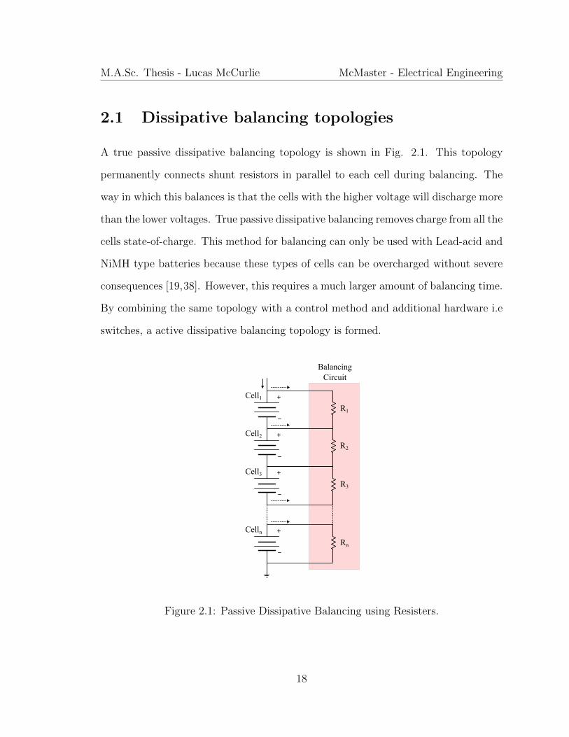
2.1 Dissipative balancing topologies
A true passive dissipative balancing topology is shown in Fig. 2.1. This topology
permanently connects shunt resistors in parallel to each cell during balancing. The
way in which this balances is that the cells with the higher voltage will discharge more
than the lower voltages. True passive dissipative balancing removes charge from all the
cells state-of-charge. This method for balancing can only be used with Lead-acid and
NiMH type batteries because these types of cells can be overcharged without severe
consequences [19,38]. However, this requires a much larger amount of balancing time.
By combining the same topology with a control method and additional hardware i.e
switches, a active dissipative balancing topology is formed.
R2
Cell2
R3
Cell3
Rn
Celln
R1
Cell1
Balancing Circuit
Figure 2.1: Passive Dissipative Balancing using Resisters.
18
M.A.Sc. Thesis - Lucas McCurlie McMaster - Electrical Engineering
R2
S2
Cell2
R3
S3
Cell3
Rn
Sn
Celln
R1
S1
Cell1
Balancing Circuit
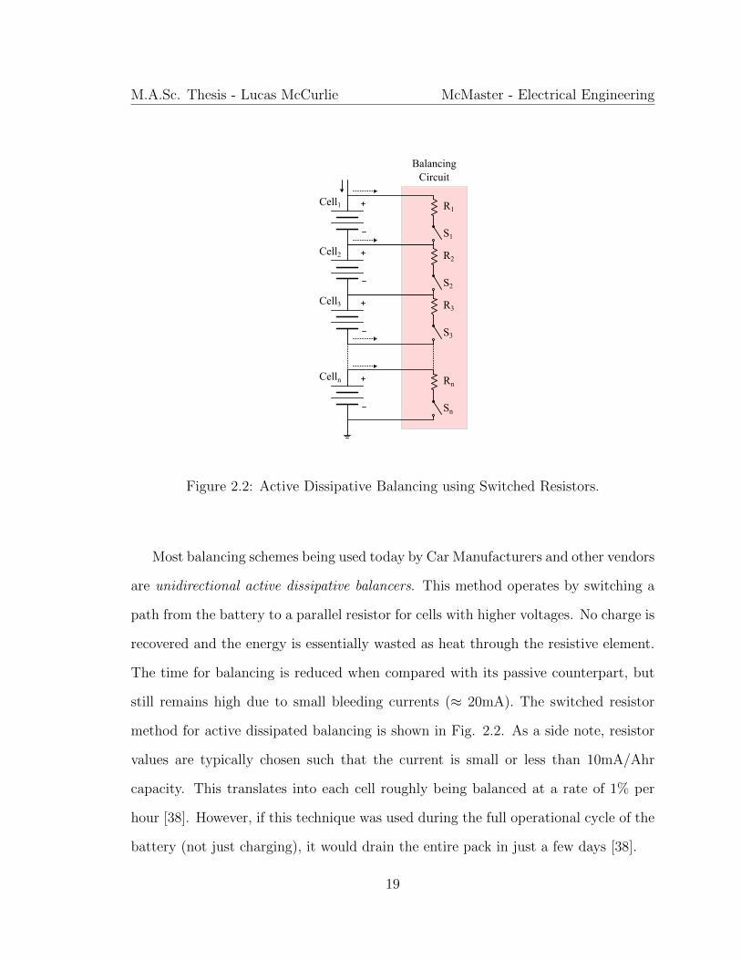
Figure 2.2: Active Dissipative Balancing using Switched Resistors.
Most balancing schemes being used today by Car Manufacturers and other vendors
are unidirectional active dissipative balancers. This method operates by switching a
path from the battery to a parallel resistor for cells with higher voltages. No charge is
recovered and the energy is essentially wasted as heat through the resistive element.
The time for balancing is reduced when compared with its passive counterpart, but
still remains high due to small bleeding currents (≈ 20mA). The switched resistor
method for active dissipated balancing is shown in Fig. 2.2. As a side note, resistor
values are typically chosen such that the current is small or less than 10mA/Ahr
capacity. This translates into each cell roughly being balanced at a rate of 1% per
hour [38]. However, if this technique was used during the full operational cycle of the
battery (not just charging), it would drain the entire pack in just a few days [38].
19
M.A.Sc. Thesis - Lucas McCurlie McMaster - Electrical Engineering
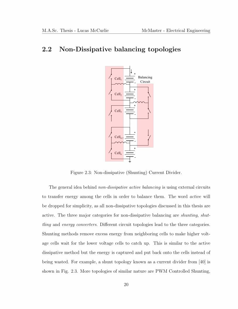
2.2 Non-Dissipative balancing topologies
Cell1
Celln-1
Cell2
Cell3
Celln
Balancing Circuit
Figure 2.3: Non-dissipative (Shunting) Current Divider.
The general idea behind non-dissipative active balancing is using external circuits
to transfer energy among the cells in order to balance them. The word active will
be dropped for simplicity, as all non-dissipative topologies discussed in this thesis are
active. The three major categories for non-dissipative balancing are shunting, shut-
tling and energy converters. Different circuit topologies lead to the three categories.
Shunting methods remove excess energy from neighboring cells to make higher volt-
age cells wait for the lower voltage cells to catch up. This is similar to the active
dissipative method but the energy is captured and put back onto the cells instead of
being wasted. For example, a shunt topology known as a current divider from [40] is
shown in Fig. 2.3. More topologies of similar nature are PWM Controlled Shunting,
20
M.A.Sc. Thesis - Lucas McCurlie McMaster - Electrical Engineering
Resonant Converter, Boost Shunting and Complete Shunting [19,38].
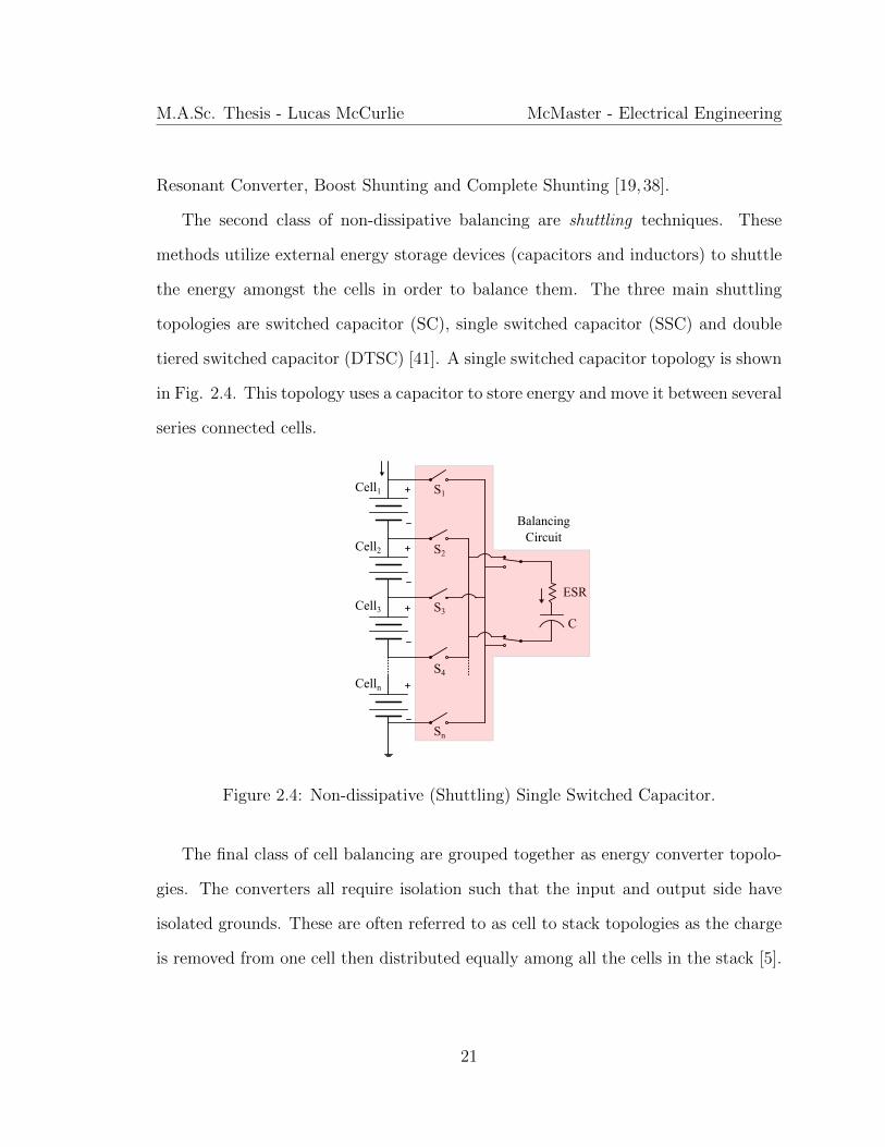
The second class of non-dissipative balancing are shuttling techniques. These
methods utilize external energy storage devices (capacitors and inductors) to shuttle
the energy amongst the cells in order to balance them. The three main shuttling
topologies are switched capacitor (SC), single switched capacitor (SSC) and double
tiered switched capacitor (DTSC) [41]. A single switched capacitor topology is shown
in Fig. 2.4. This topology uses a capacitor to store energy and move it between several
series connected cells.
Cell2
Cell3
Celln
Cell1
S2
S3
Sn
S1
Balancing Circuit
C
ESR
S4
Figure 2.4: Non-dissipative (Shuttling) Single Switched Capacitor.
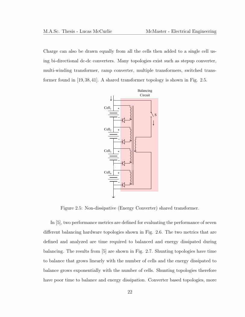
The final class of cell balancing are grouped together as energy converter topolo-
gies. The converters all require isolation such that the input and output side have
isolated grounds. These are often referred to as cell to stack topologies as the charge
is removed from one cell then distributed equally among all the cells in the stack [5].
21
M.A.Sc. Thesis - Lucas McCurlie McMaster - Electrical Engineering
Charge can also be drawn equally from all the cells then added to a single cell us-
ing bi-directional dc-dc converters. Many topologies exist such as stepup converter,
multi-winding transformer, ramp converter, multiple transformers, switched trans-
former found in [19,38,41]. A shared transformer topology is shown in Fig. 2.5.
S
Balancing Circuit
Cell1
Cell2
Cell3
Celln
Figure 2.5: Non-dissipative (Energy Converter) shared transformer.
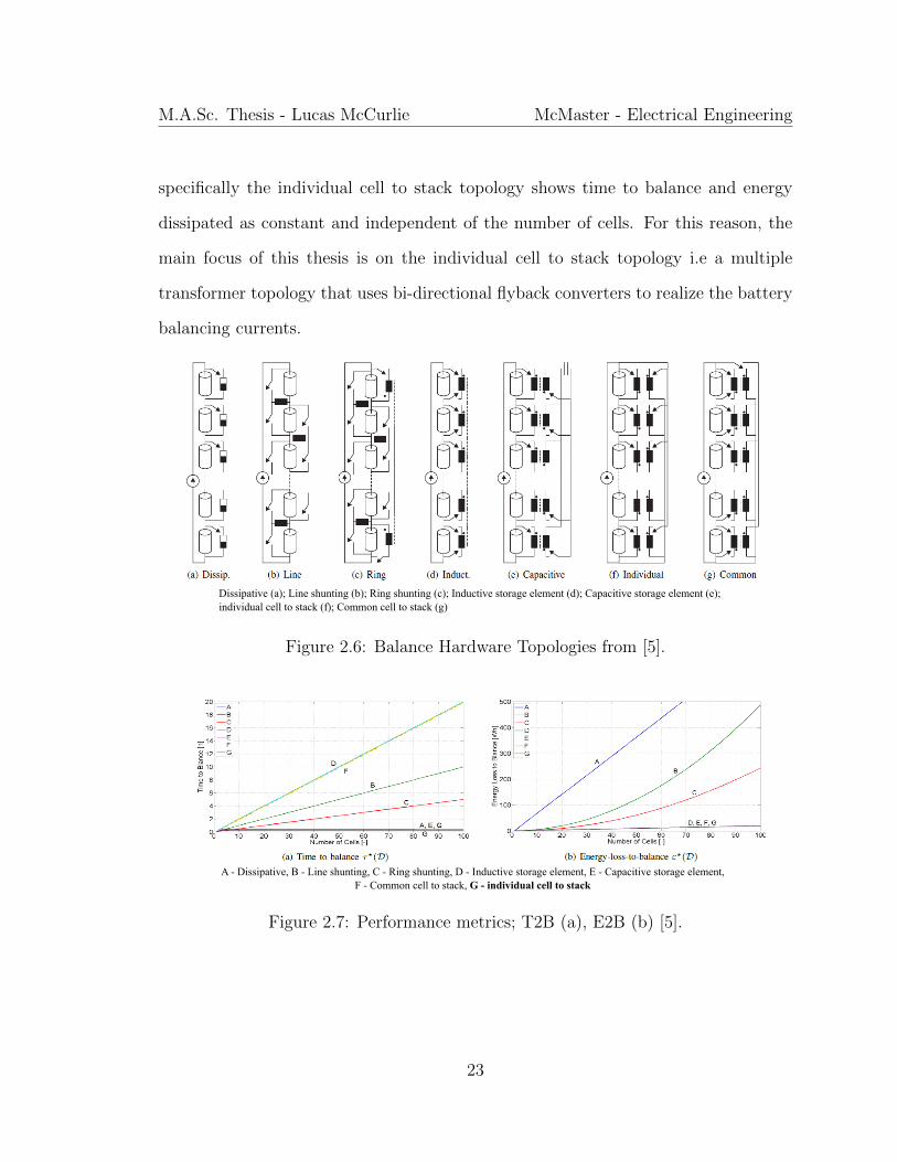
In [5], two performance metrics are defined for evaluating the performance of seven
different balancing hardware topologies shown in Fig. 2.6. The two metrics that are
defined and analyzed are time required to balanced and energy dissipated during
balancing. The results from [5] are shown in Fig. 2.7. Shunting topologies have time
to balance that grows linearly with the number of cells and the energy dissipated to
balance grows exponentially with the number of cells. Shunting topologies therefore
have poor time to balance and energy dissipation. Converter based topologies, more
22
M.A.Sc. Thesis - Lucas McCurlie McMaster - Electrical Engineering
specifically the individual cell to stack topology shows time to balance and energy
dissipated as constant and independent of the number of cells. For this reason, the
main focus of this thesis is on the individual cell to stack topology i.e a multiple
transformer topology that uses bi-directional flyback converters to realize the battery
balancing currents.
Dissipative (a); Line shunting (b); Ring shunting (c); Inductive storage element (d); Capacitive storage element (e); individual cell to stack (f); Common cell to stack (g)
Figure 2.6: Balance Hardware Topologies from [5].
A - Dissipative, B - Line shunting, C - Ring shunting, D - Inductive storage element, E - Capacitive storage element, F - Common cell to stack, G - individual cell to stack
Figure 2.7: Performance metrics; T2B (a), E2B (b) [5].
23
Chapter 3
Power Electronics used for
Redistributive Battery Balancing
3.1 Overview of Power Electronics
Power electronics is a way of controlling and converting electric power. More specif-
ically, it is the study of switching electronic circuits for the purpose of controlling
energy flow. Different classifications are made depending on the type of input and
output power requirements. A rectifier converts alternating current (AC) to direct
current (DC) and is found in many consumer products such as Televisions and Per-
sonal computers. Contrast to the rectifier is a power inverter which converts DC to
AC. System design includes parameters such as input voltage, output voltage, fre-
quency and power requirements. Many inverter applications exist such as the use
in solar panels. A AC-to-AC converter is one that converts a AC line input to AC
inverter output. A very common example of this is used in Variable frequency drives
found in electro-mechanical drive systems to control AC motor speed and torque.
24
M.A.Sc. Thesis - Lucas McCurlie McMaster - Electrical Engineering
3.2 DC-to-DC Converters
The final class in power electronics is DC-to-DC converters which convert one DC
voltage level to another. The power levels can range from very low such as in small
battery applications, to very high such as in high-voltage power transmission. Low
power level applications can be found in cell phones and laptop computers (5 - 10V).
High power level applications are Electric vehicles(300V+). In many electrical de-
vices, a large number of sub-circuits exist that require different voltage levels. Instead
of using many batteries with different input voltages, a single source is typically used
in conjunction with switched DC-to-DC converters to either increase or decrease the
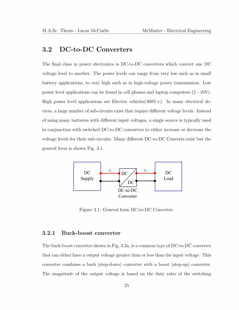
voltage levels for their sub-circuits. Many different DC-to-DC Converts exist but the
general form is shown Fig. 3.1.
DC Supply
DC Load
DC
DC
DC-to-DCConverter
V1 V2
Figure 3.1: General form DC-to-DC Converter.
3.2.1 Buck-boost converter
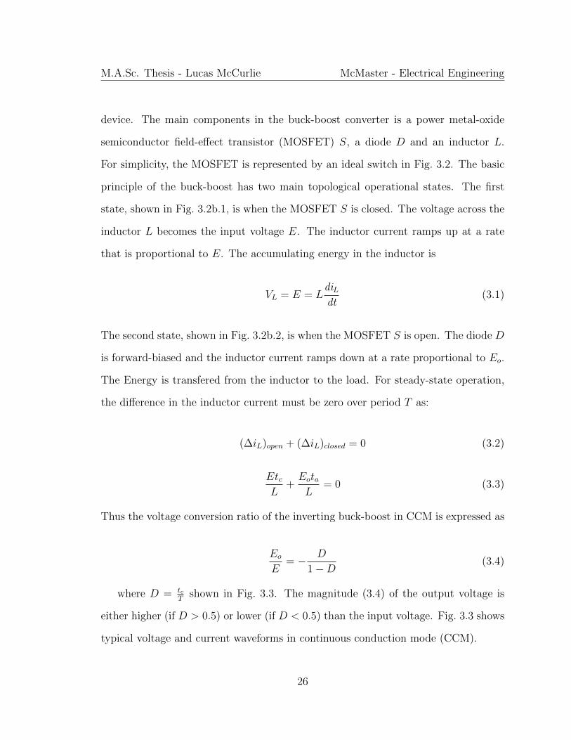
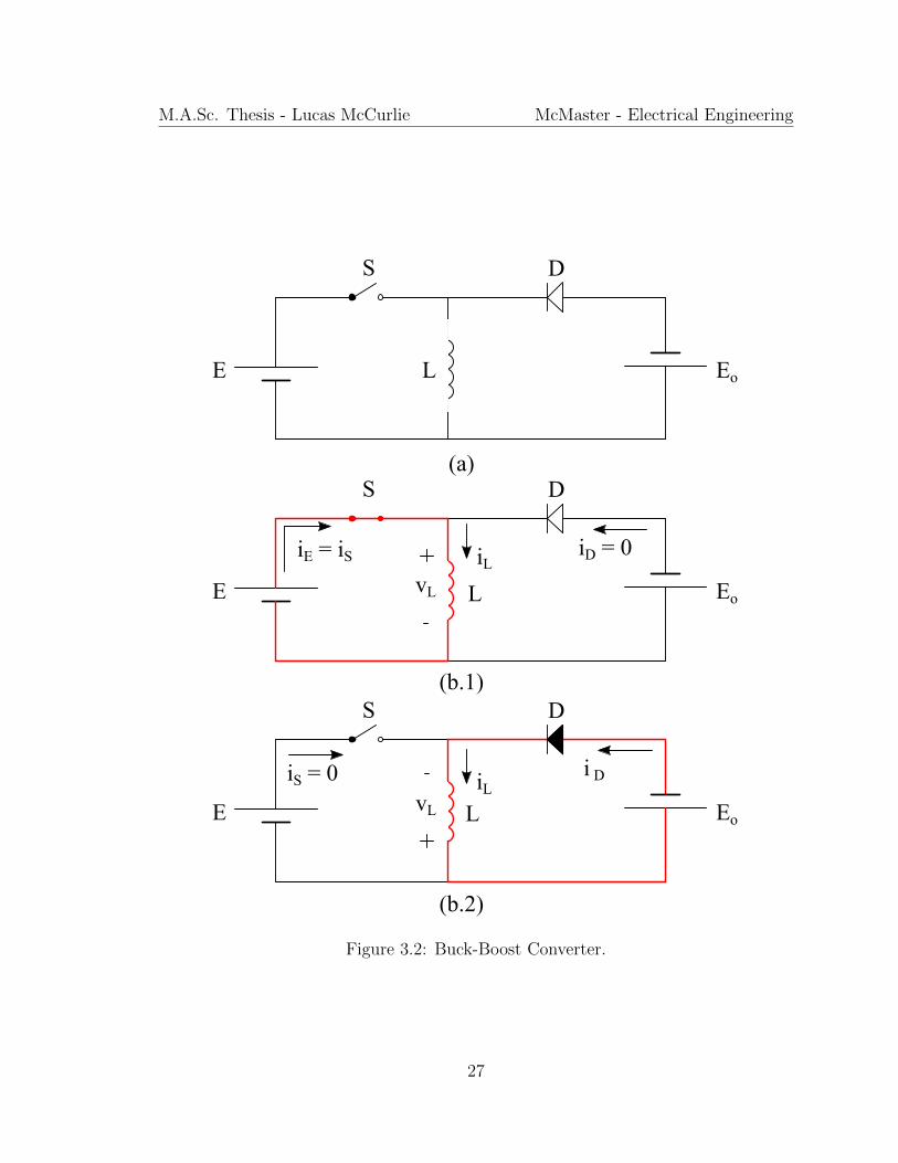
The buck-boost converter shown in Fig. 3.2a, is a common type of DC-to-DC converter
that can either have a output voltage greater than or less than the input voltage. This
converter combines a buck (step-down) converter with a boost (step-up) converter.
The magnitude of the output voltage is based on the duty ratio of the switching
25
M.A.Sc. Thesis - Lucas McCurlie McMaster - Electrical Engineering
device. The main components in the buck-boost converter is a power metal-oxide
semiconductor field-effect transistor (MOSFET) S, a diode D and an inductor L.
For simplicity, the MOSFET is represented by an ideal switch in Fig. 3.2. The basic
principle of the buck-boost has two main topological operational states. The first
state, shown in Fig. 3.2b.1, is when the MOSFET S is closed. The voltage across the
inductor L becomes the input voltage E. The inductor current ramps up at a rate
that is proportional to E. The accumulating energy in the inductor is
VL = E = LdiLdt
(3.1)
The second state, shown in Fig. 3.2b.2, is when the MOSFET S is open. The diode D
is forward-biased and the inductor current ramps down at a rate proportional to Eo.
The Energy is transfered from the inductor to the load. For steady-state operation,
the difference in the inductor current must be zero over period T as:
(∆iL)open + (∆iL)closed = 0 (3.2)
EtcL
+EotaL
= 0 (3.3)
Thus the voltage conversion ratio of the inverting buck-boost in CCM is expressed as
EoE
= − D
1−D(3.4)
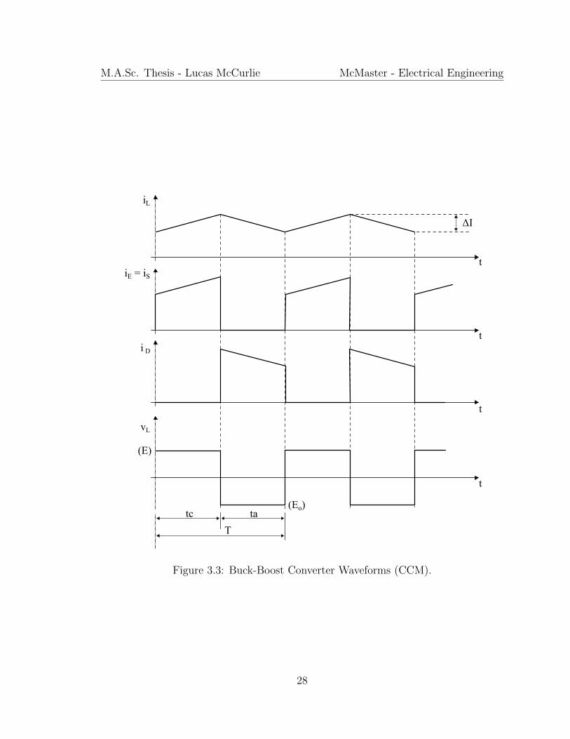
where D = tcT
shown in Fig. 3.3. The magnitude (3.4) of the output voltage is
either higher (if D > 0.5) or lower (if D < 0.5) than the input voltage. Fig. 3.3 shows
typical voltage and current waveforms in continuous conduction mode (CCM).
26
M.A.Sc. Thesis - Lucas McCurlie McMaster - Electrical Engineering
E
S
L
D
Eo
E
S
L
D
Eo
E
S
L
D
Eo
(a)
(b.1)
(b.2)
iE = iS
vL
iD = 0iL
i DiLvL
iS = 0
Figure 3.2: Buck-Boost Converter.
27
M.A.Sc. Thesis - Lucas McCurlie McMaster - Electrical Engineering
t
t
t
t
T
tc ta
(E)
vL
i D
iE = iS
iL
ΔI
(Eo)
Figure 3.3: Buck-Boost Converter Waveforms (CCM).
28
M.A.Sc. Thesis - Lucas McCurlie McMaster - Electrical Engineering
3.2.2 Flyback converter
To achieve galvanic isolation, safety, and enhanced noise immunity, the secondary
side is electrically isolated from the primary side in a isolated DC/DC converter.
This isolation is typically used in EVs to keep the power rating of the switches low
[5]. The Flyback converter provides a simple implementation for the redistributive
non-dissipated balancing system and has similar inter workings as the buck-boost
converter.
The Flyback is commonly used at 50-100W power range but still functions as high
voltage power supplies for televisions and computer monitors. Its main advantage is
in a low number of components [42] when compared to other isolated topologies.
These converter can operate in either Continuous Conduction Mode (CCM) or Dis-
continuous Conduction Mode (DCM). For the multiple transformer topology in the
redistributive non-dissipative balancer, they will be operated in Discontinuous Con-
duction Mode (DCM) because it requires a smaller transformer, reducing system
costs than its Continuous Conduction Mode (CCM) counterpart [6]. Additional volt-
age on the primary side transformer may be viewed due to ringing associated with
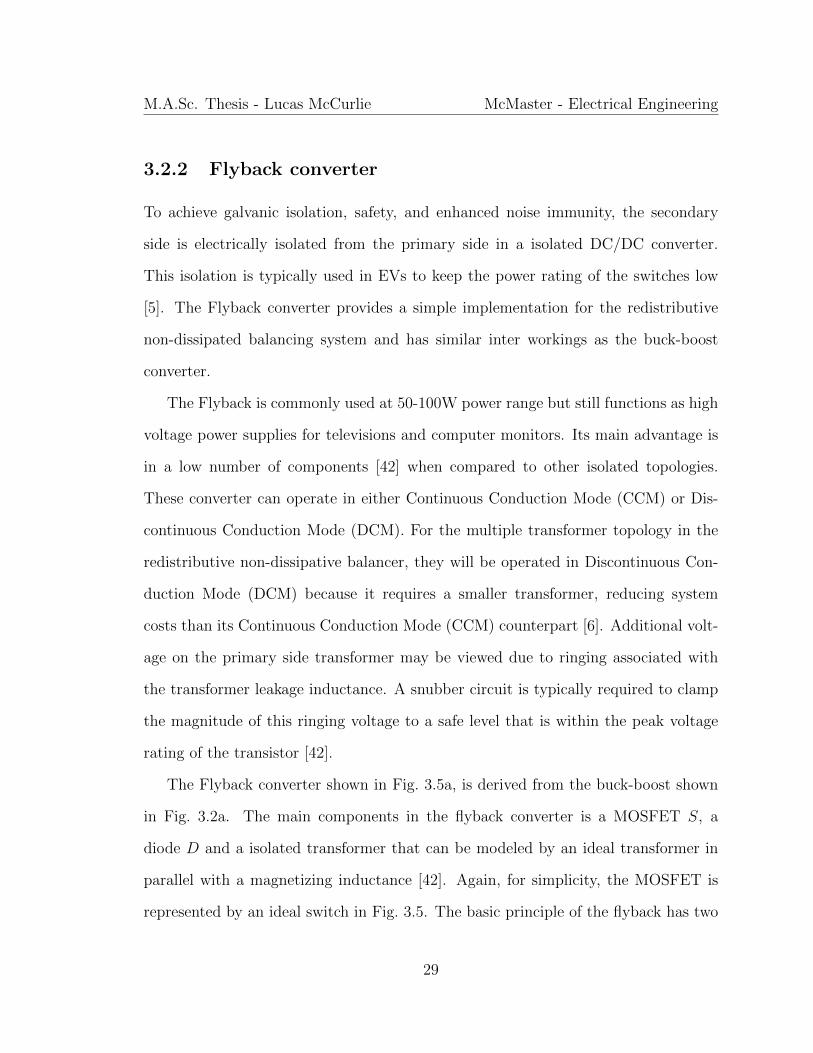
the transformer leakage inductance. A snubber circuit is typically required to clamp
the magnitude of this ringing voltage to a safe level that is within the peak voltage
rating of the transistor [42].
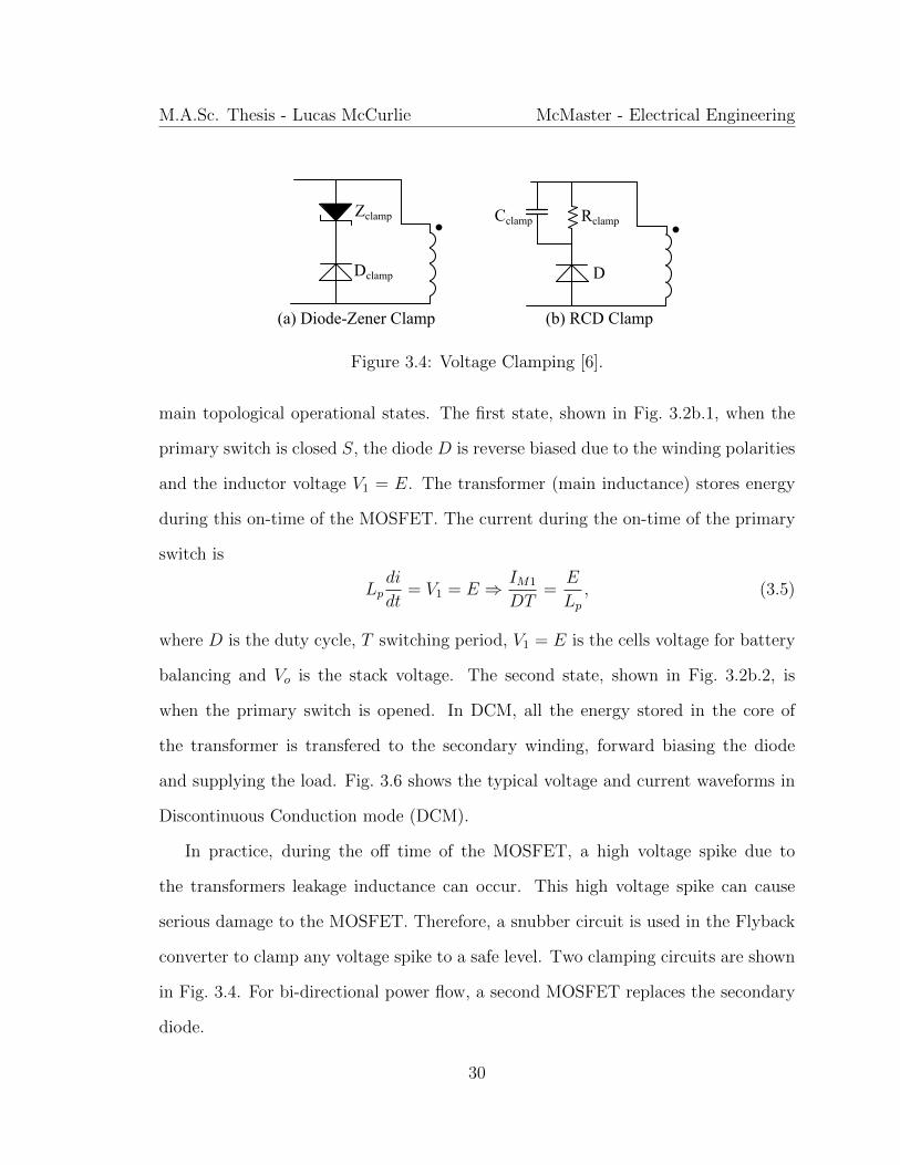
The Flyback converter shown in Fig. 3.5a, is derived from the buck-boost shown
in Fig. 3.2a. The main components in the flyback converter is a MOSFET S, a
diode D and a isolated transformer that can be modeled by an ideal transformer in
parallel with a magnetizing inductance [42]. Again, for simplicity, the MOSFET is
represented by an ideal switch in Fig. 3.5. The basic principle of the flyback has two
29
M.A.Sc. Thesis - Lucas McCurlie McMaster - Electrical Engineering
Dclamp
Zclamp
(a) Diode-Zener Clamp
D
Rclamp
(b) RCD Clamp
Cclamp
Figure 3.4: Voltage Clamping [6].
main topological operational states. The first state, shown in Fig. 3.2b.1, when the
primary switch is closed S, the diode D is reverse biased due to the winding polarities
and the inductor voltage V1 = E. The transformer (main inductance) stores energy
during this on-time of the MOSFET. The current during the on-time of the primary
switch is
Lpdi
dt= V1 = E ⇒ IM1
DT=
E
Lp, (3.5)
where D is the duty cycle, T switching period, V1 = E is the cells voltage for battery
balancing and Vo is the stack voltage. The second state, shown in Fig. 3.2b.2, is
when the primary switch is opened. In DCM, all the energy stored in the core of
the transformer is transfered to the secondary winding, forward biasing the diode
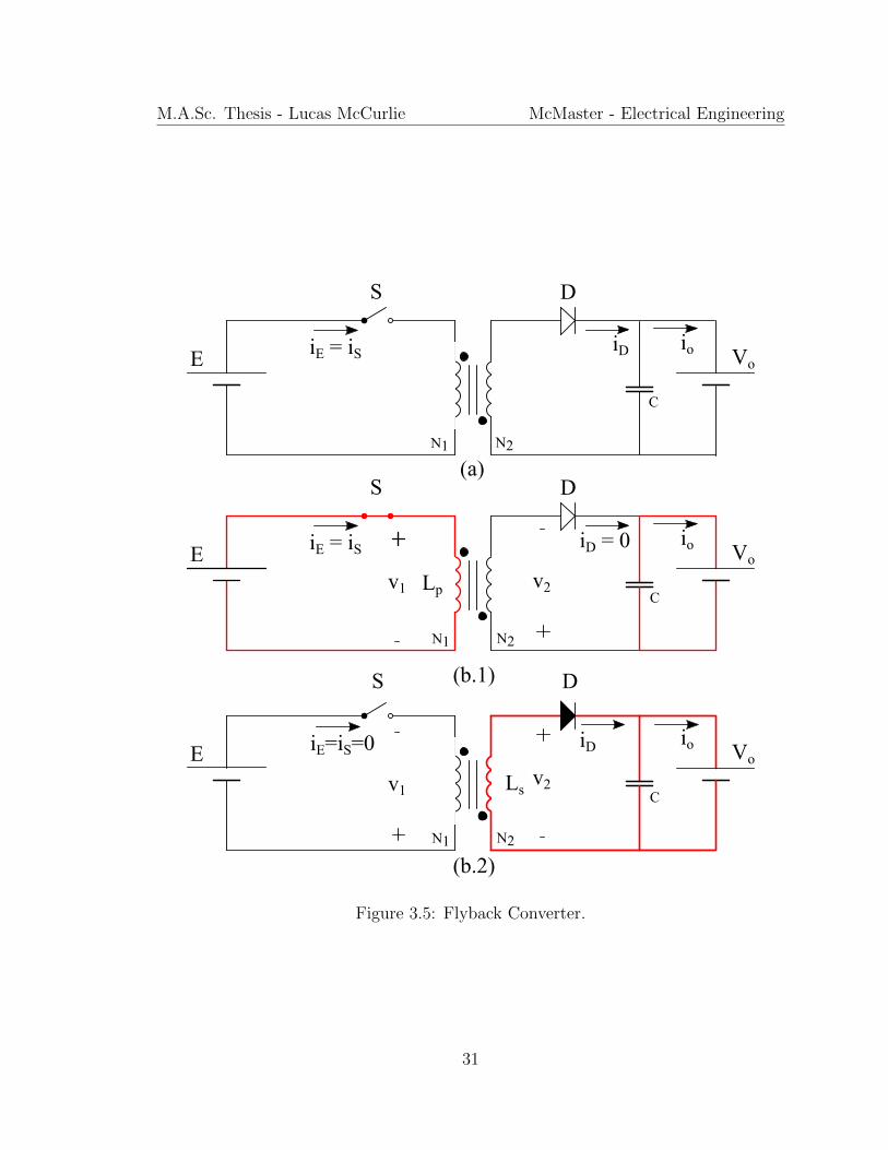
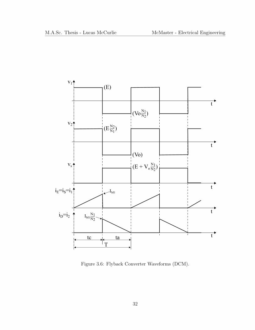
and supplying the load. Fig. 3.6 shows the typical voltage and current waveforms in
Discontinuous Conduction mode (DCM).
In practice, during the off time of the MOSFET, a high voltage spike due to
the transformers leakage inductance can occur. This high voltage spike can cause
serious damage to the MOSFET. Therefore, a snubber circuit is used in the Flyback
converter to clamp any voltage spike to a safe level. Two clamping circuits are shown
in Fig. 3.4. For bi-directional power flow, a second MOSFET replaces the secondary
diode.
30
M.A.Sc. Thesis - Lucas McCurlie McMaster - Electrical Engineering
(a)
(b.2)
S D
Vo
N1 N2
C
EiDiE = iS
io
S D
VoE iD = 0iE = iS
io
N1 N2
Cv1 Lp v2
DS
VoE iDiE=iS=0 io
N1 N2
Cv1 Ls
v2
(b.1)
Figure 3.5: Flyback Converter.
31
M.A.Sc. Thesis - Lucas McCurlie McMaster - Electrical Engineering
t
t
t
t
iE=iS=i1
v1(E)
(Vo )N1N2
v2(E )
(Vo)
N1
N2
vs (E + Vo )N1N2
IM1
iD=i2 IM1N1N2
Ttc ta t
Figure 3.6: Flyback Converter Waveforms (DCM).
32
Chapter 4
Control Techniques, Analysis and
Design
High level cell balancing can be achieved using either voltage based input or state-of-
charge based input. Voltage based methods use simple hardware thus making their
implementation easier, but suffer from slower balancing speeds and possibly introduc-
ing further imbalances due to distortions from impedance differences [43]. SoC based
methods are much more complicated but are more accurate and faster to balance [43].
In this thesis, a top level controller balances the cells state-of-charge using actuating
currents in the links. The state-of-charge x is not measurable but can be estimated
according to y = C(x) where y is the voltage associated with the battery terminals
and C is some nonlinear mapping [24]. Kalman filters [25], neural networks [26], elec-
trochemical impedance spectroscopy [27] and fuzzy logic [28, 29] are all examples of
advanced methods for SoC estimation. This Chapter assumes SoC is constructed with
sufficient precision. In this Chapter, different balancing control methods are identi-
fied and developed. These methods include a unconstrained optimization problem
33
M.A.Sc. Thesis - Lucas McCurlie McMaster - Electrical Engineering
using a Linear Quadratic Regulator (LQR) and finally a constrained optimization
problem using Model Predictive Control (MPC). These methods are benchmarked
against traditional rule based (RB) balancing.
4.1 Battery System Description
A description for the overall system must first be defined before developing the con-
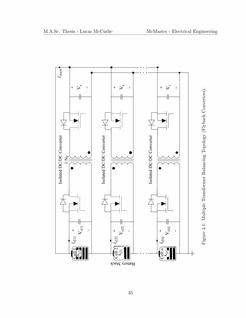
trol algorithms. The redistributive non-dissipative balancing system known as the
Multiple Transformer topology is shown Fig. 4.1. The battery pack is defined by n
series connected battery cells with m number of links. Each cell is described by the
amount of remaining charge via Qx ∈ Rn. The matrix
Q =
C1 0 . . . 0
0 C2 . . . 0
......
...
0 0 . . . Cn
∈ Rnxn
is a diagonal matrix that defines each cells maximum charge capacities (C in Ah) and
x is the state-of-charge vector
x =
[x1 x2 . . . xn
]>∈ Rn.
Each element in the SoC vector ranges between zero and one where the value of 0
corresponds to a completely empty cell and the value of 1 corresponds to a fully
charged cell. For the system to become balanced, charge is moved between m links.
The balancing current being transfered through the links is Au ∈ Rm where u is a
34
M.A.Sc. Thesis - Lucas McCurlie McMaster - Electrical Engineering
Cel
l 1
1:N
r
Isol
ated
DC
/DC
Con
vert
eri stack
x [1]
Vs
Vs
Vs
Cel
l 2x [
2]
Cel
l nx [n]
Vc[
2]
Vc[
1]
Vc[n]
i c[1
]
i c[2
]
i c[n
]
Battery Stack
Isol
ated
DC
/DC
Con
vert
er
Isol
ated
DC
/DC
Con
vert
er
Fig
ure
4.1:
Mult
iple
Tra
nsf
orm
erB
alan
cing
Top
olog
y(F
lybac
kC
onve
rter
s).
35
M.A.Sc. Thesis - Lucas McCurlie McMaster - Electrical Engineering
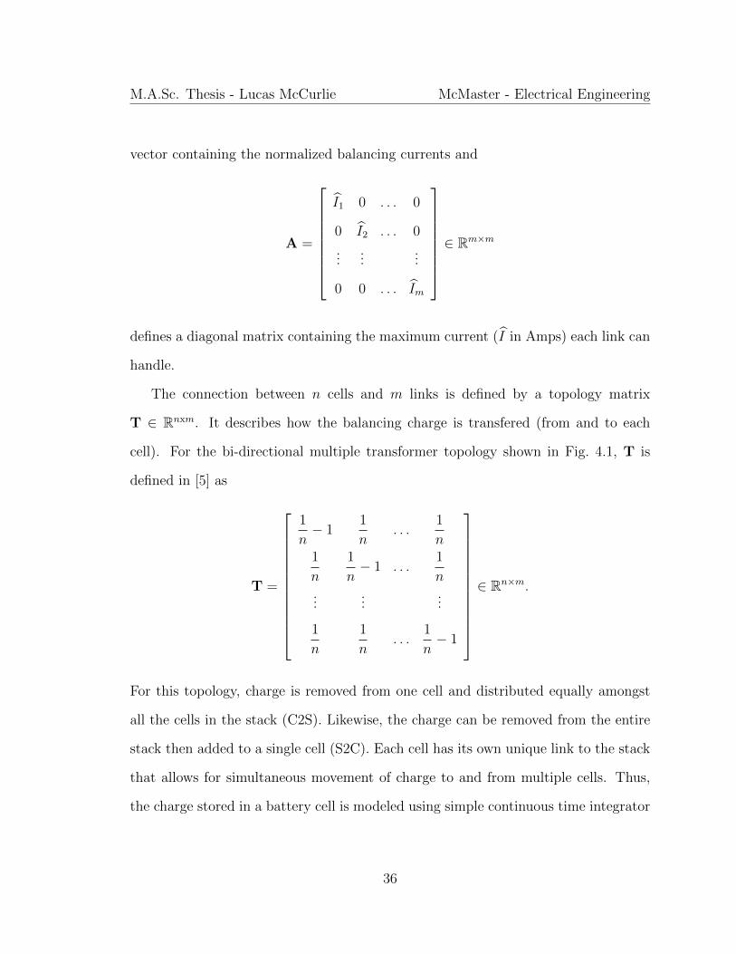
vector containing the normalized balancing currents and
A =
I1 0 . . . 0
0 I2 . . . 0
......
...
0 0 . . . Im
∈ Rm×m
defines a diagonal matrix containing the maximum current (I in Amps) each link can
handle.
The connection between n cells and m links is defined by a topology matrix
T ∈ Rnxm. It describes how the balancing charge is transfered (from and to each
cell). For the bi-directional multiple transformer topology shown in Fig. 4.1, T is
defined in [5] as
T =
1
n− 1
1
n. . .
1
n1
n
1
n− 1 . . .
1
n...
......
1
n
1
n. . .
1
n− 1
∈ Rn×m.
For this topology, charge is removed from one cell and distributed equally amongst
all the cells in the stack (C2S). Likewise, the charge can be removed from the entire
stack then added to a single cell (S2C). Each cell has its own unique link to the stack
that allows for simultaneous movement of charge to and from multiple cells. Thus,
the charge stored in a battery cell is modeled using simple continuous time integrator
36
M.A.Sc. Thesis - Lucas McCurlie McMaster - Electrical Engineering
dynamics as
Qx(t) = TAu(t), (4.1)
where the topology matrix T relates the normalized balancing currents u(t) with the
SoC x(t). A sign convention of u(t) > 0 indicates a flow of charge from the cell to
the stack and u(t) < 0 indicates a flow of charge from the stack the cell. Since T, A,
Q are all constants, the system dynamics can be simplified to
x(t) = Bu(t), (4.2)
where B = Q−1TAu. With the addition of the topology matrix T, equation 4.2 is
identical to equation 1.1 but has been expanded for multiple cells. The maximum
rated link current limits the applied balancing current. These balancing currents are
subject to polyhedral constraints that depend on the topology [5] [44]. The inequality
constraint is based on the maximum amount of current through each link |u(t)| ≤ 1.
From Proposition 1 [5] there exists a constant input trajectory u(t) = u. Thus, the
state-of-charge is further simplified to just
x+ = x+ TsBu, (4.3)
where Ts is the sampling period and u is the normalized balancing currents found by
each control method.
37
M.A.Sc. Thesis - Lucas McCurlie McMaster - Electrical Engineering
4.2 LQR Control
This method is first described in [37] but is expanded upon in this Thesis. The
constraints for the system are written as Hu ≤ K for the inequality constraint and
Hequ = Keq for the equality constraint. For the LQR control to function, the equality
constraint on the system dynamics is defined by transforming (4.3) into a regulation
problem using the transformation matrix
L =
1 −1 0 . . . 0 0
0 1 −1 . . . 0 0
......
......
...
0 0 0 . . . 1 −1
∈ R(n−1)×n.
This matrix L leaves the difference in SoC between neighboring cells. Thus the
regulation problem uses x = Lx and the balanced state is when x = 0. The equality
constraint is removed using the transformation
u = Fu′ + u0, (4.4)
where F is the nullspace of Heq, such that FHeq ≡ 0 and u0 is any solution of Hequ0 =
Keq. This will yield the system
x+ = x+ Bu′ + LBu0, (4.5)
where B = LBF. The component LBu0 is a non-zero offset value in general that
can be removed by integration. However, LBu0 ≡ 0 for all topologies studied in [5].
38
M.A.Sc. Thesis - Lucas McCurlie McMaster - Electrical Engineering
The updated system (4.5) is linear, thus a discrete, infinite-time Linear Quadratic
Regulator (LQR) that minimizes the cost function J =∑∞
k=0(xTkQxk + uTkRuk) is
used.
The LQR problem is solved by a regular feedback controller defined as
u′ = −Klqrx, (4.6)
where Klqr is found by solving the discrete time Riccati equation. However, the con-
troller input may not satisfy the inequality constraints. Thus, the input is saturated
such that it satisfies the inequality constrains according to
Hu ≤ K, (4.7)
where H = HF and K = K −Hu0. The result is transformed into a control input
for the original system with (4.4). The saturation (4.7) ensures that the inequality
constraints are satisfied and the transformation (4.4) ensures that the equality con-
straints are met. Meaning that the resulting back-transformed u is feasible. Also,
the resulting closed loop system is stable according to [45] [46]. The LQR now has a
control input u that defines the balancing currents in each link as
Au = [ic1 , ic2 , ic3 ...icm ]. (4.8)
39
M.A.Sc. Thesis - Lucas McCurlie McMaster - Electrical Engineering
4.3 MPC Control
In [5] performance metrics have been developed to evaluate hardware. This thesis
uses the minimum time to balance (t2b) metric as a balancing control. Defining this
control is not as straight forward as LQR because it not only has to determine the
normalized balancing currents, but must do so such that the balancing occurs in the
minimum amount of time τ . Thus, a battery cells state of charge in terms of a control
input at the final balancing time τ , is
x(τ) = x(0) + B
∫ τ
0
u(t)dt. (4.9)
From Proposition 1 [5] there exists a constant input trajectory u(t) = u such
that
x(τ) = x(0) + Buτ. (4.10)
Much like the LQR method, the constraints for the system are written as Hu ≤ K for
the inequality constraint and Hequ = Keq for the equality constraint. The equality
constraint on the system dynamics is defined by transforming (4.10) into a regulation
problem. However, with MPC the transformation matrix is
L = I− J (4.11)
where I ∈ Rnxn is the identity matrix and J ∈ Rnxn is a matrix containing all 1/n
elements. This removes the average SoC and leaves the unbalanced SoC. The equality
40
M.A.Sc. Thesis - Lucas McCurlie McMaster - Electrical Engineering
constraint now becomes
Lx(0) + LBuτ = Lx(τ) = 0. (4.12)
The constraints for the system are written as Hu ≤ K for the inequality constraint
and Hequ = Keq for the equality constraint. The constrained linear optimization
problem is formally expressed as
τ ?(x) = minimizeτ≥0
τ (4.13a)
subject to Lx+ LBuτ = 0 (4.13b)
Huτ −Kτ ≤ 0 (4.13c)
To efficiently solve (4.13a) using popular Linear programming solver packages such
as LPSOLVE, CPLEX or MOSEK, it is worth reproducing the problem in standard
form. This is achieved by defining a new column vector containing both variables
z =
v
τ
,where v = uτ . It is important to realize that Lx is a parameter and is treated as a
constant. The minimum time to balance problem (4.13a) in standard form becomes
z? = minimize g′z (4.14a)
subject to Aeqz = beq (4.14b)
Az ≤ b (4.14c)
41
M.A.Sc. Thesis - Lucas McCurlie McMaster - Electrical Engineering
where Aeq = [LB 0], beq = [−Lx 0], A = [H− k], b = 0.
Many simple solvers are more efficient when dealing without equality constraints
such as qpOASES. This is not mandatory but by removing the equality constraint
from (4.14a), the dimensions of the optimization problem are reduced.
To do this, the following linear transformation is used
z = Fz + z0 (4.15)
where F is the nullspace of Aeq, such that FAeq ≡ 0 and z0 is any solution of Aeqz0 =
beq. Equation (4.15) is substituted into (4.14a) to ensure that the equality constraint
is still satisfied but is now removed from the problem. Thus, a formal definition for
the minimum time to balance problem in standard form with the removed equality
constraint is
z? = minimize g′z (4.16a)
subject to Az ≤ b (4.16b)
where A = AF, b = b−Azo.
The performance metric is now used to define a model predictive controller. To
adapt this into a discrete time MPC controller, equation (4.16a) is solved for the
optimal τ ∗ and u∗ at each sampling time instant kTs using the discrete time dynamics
Lx+ LBuτ = 0. (4.17)
Then a scaling factor ν is introduced to scale down the control if τ ∗ is smaller than the
42
M.A.Sc. Thesis - Lucas McCurlie McMaster - Electrical Engineering
sampling period Ts such that the process leads to the following closed loop dynamics
x[k + 1] = x[k] + νTsBu∗[k] (4.18)
where
ν =
τ∗
Tsfor τ ∗ ≤ Ts
1 for τ ∗ > Ts
(4.19)
This sequence is repeated for each sampling instant until the system becomes bal-
anced, i.e Lx[k] = 0.
4.4 Rule based Control
Rule based control methods use a set of rules to manipulate some form of outcome
in a system. Examples of RB in other EV applications are found in [47–49]. For a
bi-directioanl (C2S/S2C) system, the average state-of-charge is defined as
x =||x||1n
(4.20)
where x is a vector containing state-of-charge and n is number of cells. If a cells x is
higher than the average x then it is discharged onto the stack i.e u = 1. Likewise, if a
cells x is lower than the average x then it is charged by the stack i.e u = −1. As a side
note, this could easily be changed for a uni-directional active dissipative approach by
balancing towards the minimum SoC. This simple control method uses the maximum
link current available i.e each cell is always charging or discharging until all cells SoC
43

M.A.Sc. Thesis - Lucas McCurlie McMaster - Electrical Engineering
fall within a ”balanced region” Bz. A transformation matrix is used
L = I− J (4.21)
where I ∈ Rnxn is the identity matrix and J ∈ Rnxn is a matrix containing all 1/n
elements. This removes the average SoC and leaves the unbalanced SoC. Thus the
balanced region Bz is defined as 5% or when
||Lx||1 < 0.05 (4.22)
The set of simple rules for redistributive non-dissipative balancing are summarized as
u =
1(Discharge) if x > x
−1(Charge) if x < x
0 if ||Lx||1 < 0.05
(4.23)
44
Chapter 5
Implementation Details
5.1 Linear Technology DC2100A Hardware
At the outset of this thesis, implementing control strategies and obtaining experi-
mental data as such was most important. For rapid prototyping and implementation,
the hardware for experimental data was built upon an existing Linear Technology
DC2100A Demonstration board [50]. This application hardware is developed for bi-
directional cell balancing of up to 12 Lithium ion cells. By monitoring the cell voltage
and protecting against over charge and under charge conditions, algorithms for State-
of-charge estimation can be embedded onto a daughter board (PIC18F47J53). This
microcontroller communicates to the LTC3300-1 and LTC6804 integrated circuits
through SPI communication.
Off the shelf this board had bi-directional flyback converters that were all con-
trolled with a convenient graphical user interface. The original Code Communication
Diagram in Fig. 5.1 shows the flow of communication such that any new software
communicates with the boot firmware through the HID windows driver. The GUI
45

M.A.Sc. Thesis - Lucas McCurlie McMaster - Electrical Engineering
Figure 5.1: DC2100A Code Communication Diagram [7].
software communicates with the Application Firmware through the WinUSB win-
dows driver. The App FW passes commands and responds to the GUI SW. The App
FW must also provide communication to the ICs and general inputs and outputs.
The main ICs on the DC2100A are the LTC6820, LTC6804-2 and LTC3300-1. The
LTC6820 IC converts SPI into isoSPI for the monitoring ICs on the DC2100A. The
LTC6804-2 IC measures battery voltage as well as passes I2C and SPI communication
to the balancing chips. The LTC3300-1 IC provides active balancing commands to
the bi-directional converters.
On the surface this board seemed to have what was required for conducting the ex-
periments with little to no modifications. However, during the initial stages of testing,
it became clear that the on-board PIC microcontroller did not have sufficient stor-
age space for any additional algorithms. Luckily, the designers at Linear Technology
made it possible to disconnect the PIC from the system then connect an alternative
solution to monitor and control the DC2100A hardware. This is done through the
JP7 header seen in the original communication diagram (Fig. 5.1). The JP7 header
is a 6 row pin configuration that interfaces with alternative microcontrollers via SPI
46
M.A.Sc. Thesis - Lucas McCurlie McMaster - Electrical Engineering
and has a pinout as follows: pin 1 - LTC6820 ENABLE, pin 2 - SPI MOSI, pin 3 -
SPI MISO, pin 4 - SPI SCK, pin 5 - SPI CS, pin 6 - GND.
5.2 Texas Instruments F28377D Controller
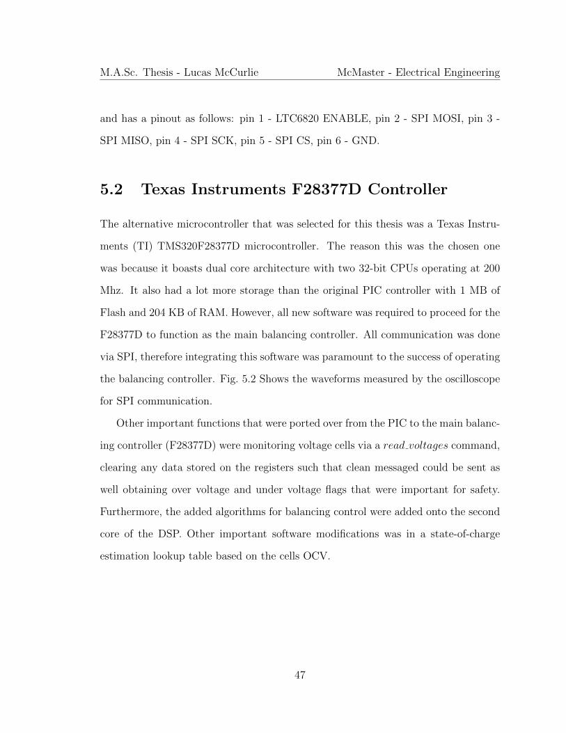
The alternative microcontroller that was selected for this thesis was a Texas Instru-
ments (TI) TMS320F28377D microcontroller. The reason this was the chosen one
was because it boasts dual core architecture with two 32-bit CPUs operating at 200
Mhz. It also had a lot more storage than the original PIC controller with 1 MB of
Flash and 204 KB of RAM. However, all new software was required to proceed for the
F28377D to function as the main balancing controller. All communication was done
via SPI, therefore integrating this software was paramount to the success of operating
the balancing controller. Fig. 5.2 Shows the waveforms measured by the oscilloscope
for SPI communication.
Other important functions that were ported over from the PIC to the main balanc-
ing controller (F28377D) were monitoring voltage cells via a read voltages command,
clearing any data stored on the registers such that clean messaged could be sent as
well obtaining over voltage and under voltage flags that were important for safety.
Furthermore, the added algorithms for balancing control were added onto the second
core of the DSP. Other important software modifications was in a state-of-charge
estimation lookup table based on the cells OCV.
47
M.A.Sc. Thesis - Lucas McCurlie McMaster - Electrical Engineering
Figure 5.2: Oscilloscope SPI protocol with TMS320F28377D and DC2100A.
48
M.A.Sc. Thesis - Lucas McCurlie McMaster - Electrical Engineering
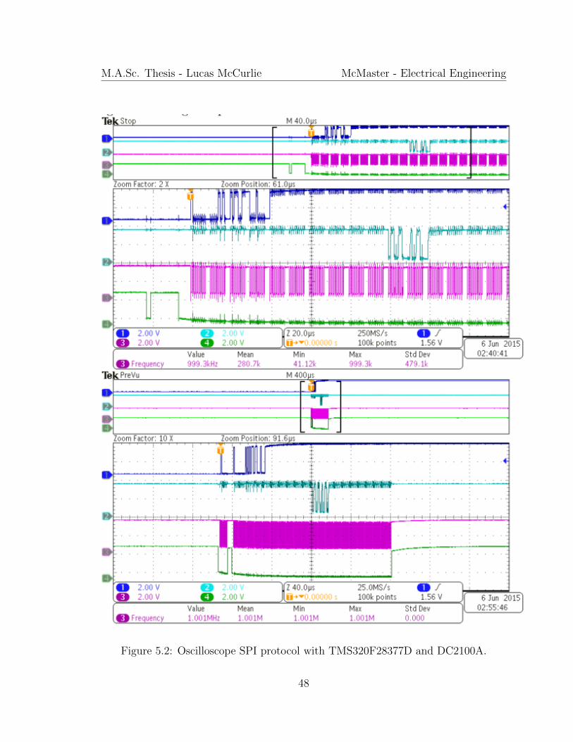
Figure 5.3: Battery Balancing 3D Graphic of Harness.
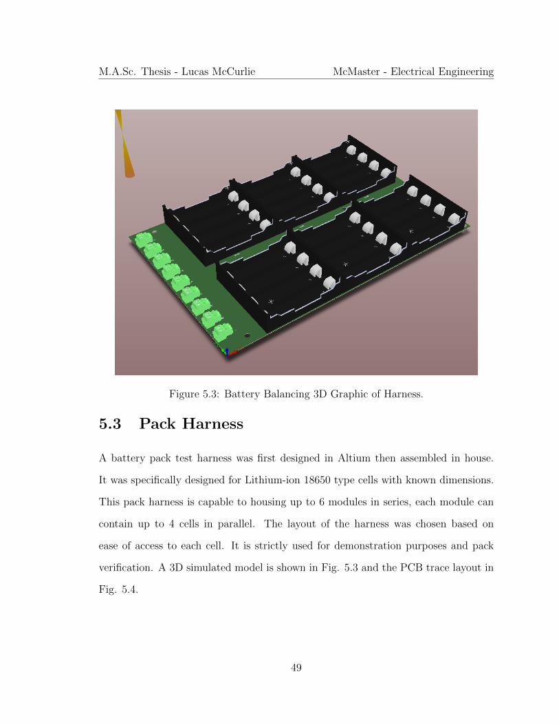
5.3 Pack Harness
A battery pack test harness was first designed in Altium then assembled in house.
It was specifically designed for Lithium-ion 18650 type cells with known dimensions.
This pack harness is capable to housing up to 6 modules in series, each module can
contain up to 4 cells in parallel. The layout of the harness was chosen based on
ease of access to each cell. It is strictly used for demonstration purposes and pack
verification. A 3D simulated model is shown in Fig. 5.3 and the PCB trace layout in
Fig. 5.4.
49
M.A.Sc. Thesis - Lucas McCurlie McMaster - Electrical Engineering
Figure 5.4: Battery test harness Altium PCB trace layout.
5.4 Full Test Bench
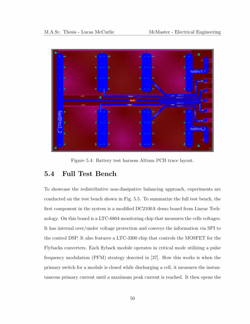
To showcase the redistributive non-dissipative balancing approach, experiments are
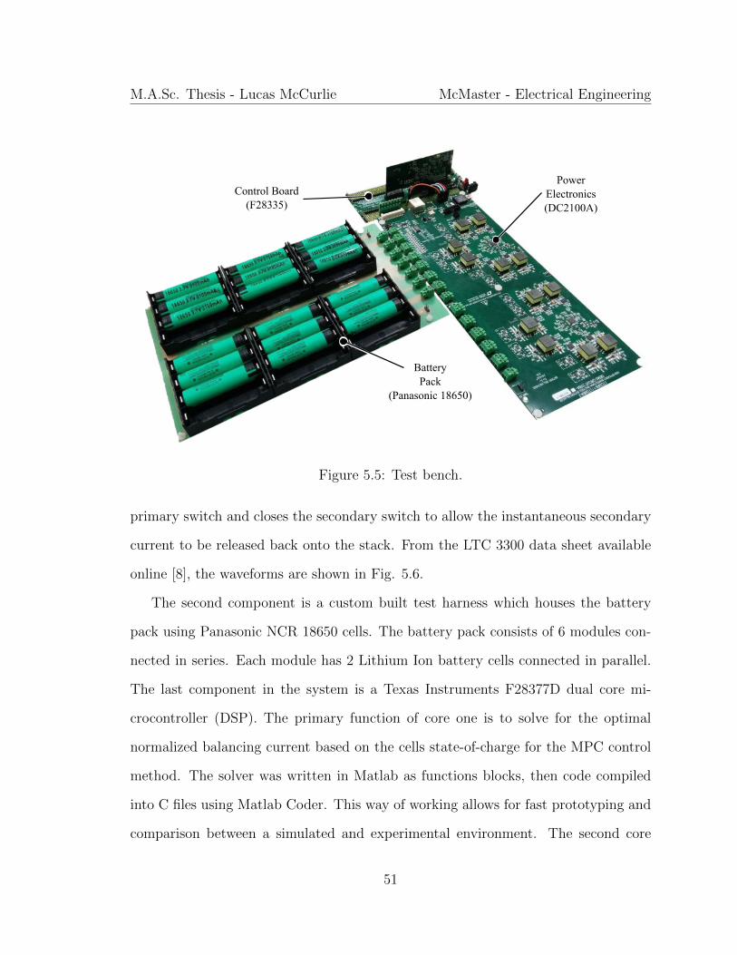
conducted on the test bench shown in Fig. 5.5. To summarize the full test bench, the
first component in the system is a modified DC2100A demo board from Linear Tech-
nology. On this board is a LTC-6804 monitoring chip that measures the cells voltages.
It has internal over/under voltage protection and conveys the information via SPI to
the control DSP. It also features a LTC-3300 chip that controls the MOSFET for the
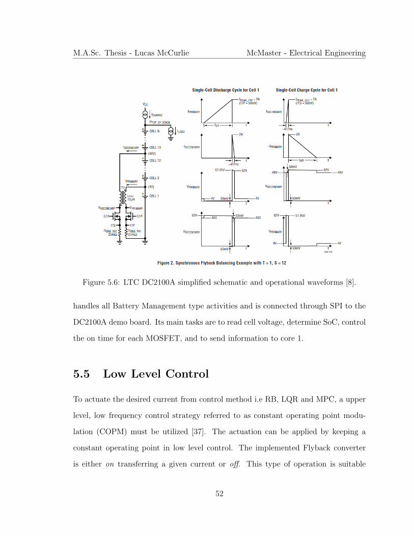
Flybacks converters. Each flyback module operates in critical mode utilizing a pulse
frequency modulation (PFM) strategy descried in [37]. How this works is when the
primary switch for a module is closed while discharging a cell, it measures the instan-
taneous primary current until a maximum peak current is reached. It then opens the
50
M.A.Sc. Thesis - Lucas McCurlie McMaster - Electrical Engineering
BatteryPack
(Panasonic 18650)
Control Board(F28335)
PowerElectronics(DC2100A)
Figure 5.5: Test bench.
primary switch and closes the secondary switch to allow the instantaneous secondary
current to be released back onto the stack. From the LTC 3300 data sheet available
online [8], the waveforms are shown in Fig. 5.6.
The second component is a custom built test harness which houses the battery
pack using Panasonic NCR 18650 cells. The battery pack consists of 6 modules con-
nected in series. Each module has 2 Lithium Ion battery cells connected in parallel.
The last component in the system is a Texas Instruments F28377D dual core mi-
crocontroller (DSP). The primary function of core one is to solve for the optimal
normalized balancing current based on the cells state-of-charge for the MPC control
method. The solver was written in Matlab as functions blocks, then code compiled
into C files using Matlab Coder. This way of working allows for fast prototyping and
comparison between a simulated and experimental environment. The second core
51
M.A.Sc. Thesis - Lucas McCurlie McMaster - Electrical Engineering
Figure 5.6: LTC DC2100A simplified schematic and operational waveforms [8].
handles all Battery Management type activities and is connected through SPI to the
DC2100A demo board. Its main tasks are to read cell voltage, determine SoC, control
the on time for each MOSFET, and to send information to core 1.
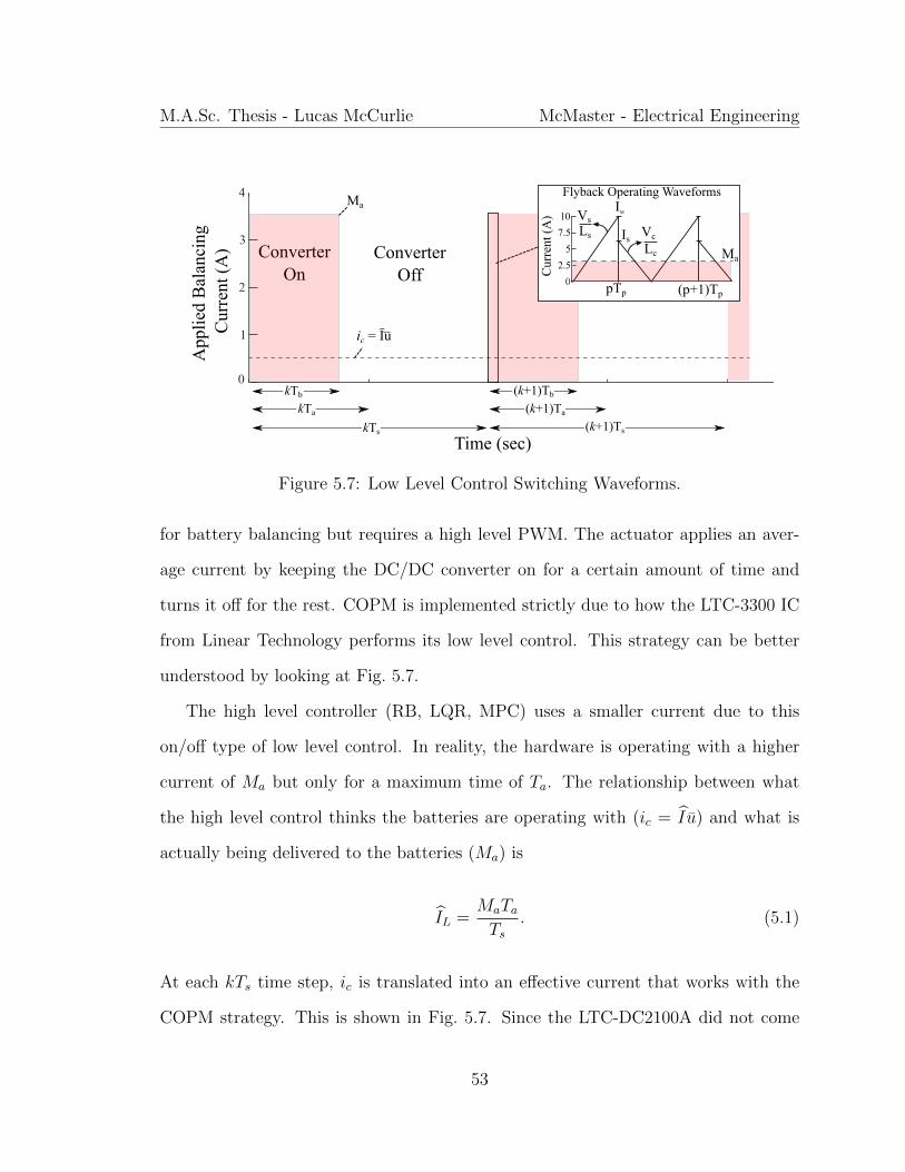
5.5 Low Level Control
To actuate the desired current from control method i.e RB, LQR and MPC, a upper
level, low frequency control strategy referred to as constant operating point modu-
lation (COPM) must be utilized [37]. The actuation can be applied by keeping a
constant operating point in low level control. The implemented Flyback converter
is either on transferring a given current or off. This type of operation is suitable
52
M.A.Sc. Thesis - Lucas McCurlie McMaster - Electrical Engineering
0
1
2
3
4Ma
App
lied
Bal
anci
ng C
urre
nt (
A)
Time (sec)
ic = Iuˆ
kTb
kTa
kTs
(k+1)Tb
(k+1)Ta
(k+1)Ts
ConverterOn
ConverterOff
Vs
Ls Vc
Lc
(p+1)TppTp
Flyback Operating Waveforms
Ma
Is
IM
10
0
2.5
5
7.5
Cur
rent
(A
)
Figure 5.7: Low Level Control Switching Waveforms.
for battery balancing but requires a high level PWM. The actuator applies an aver-
age current by keeping the DC/DC converter on for a certain amount of time and
turns it off for the rest. COPM is implemented strictly due to how the LTC-3300 IC
from Linear Technology performs its low level control. This strategy can be better
understood by looking at Fig. 5.7.
The high level controller (RB, LQR, MPC) uses a smaller current due to this
on/off type of low level control. In reality, the hardware is operating with a higher
current of Ma but only for a maximum time of Ta. The relationship between what
the high level control thinks the batteries are operating with (ic = I u) and what is
actually being delivered to the batteries (Ma) is
IL =MaTaTs
. (5.1)
At each kTs time step, ic is translated into an effective current that works with the
COPM strategy. This is shown in Fig. 5.7. Since the LTC-DC2100A did not come
53
M.A.Sc. Thesis - Lucas McCurlie McMaster - Electrical Engineering
equipped with average link current sensors, estimated current equations provide a
close approximation of the average link current through each flyback converter [37].
While a cell is being discharged, the estimated current through the link is
id =IMVs
2(Vs +NrVc). (5.2)
While a cell is being charged, the estimated current through the link is
ic =ISNrVs
2(Vs +NrVc). (5.3)
The values of the estimated currents are then scaled with the maximum operating
link current Ma. These calculations are performed by the DSP in order to control
how long each switch is on for Tb to achieve the same effective current the fast MPC
controller requires. This on-time is calculated as
Tb =
uMaTa
idfor u > 0
−uMaTa
icfor u < 0
0 for u = 0
(5.4)
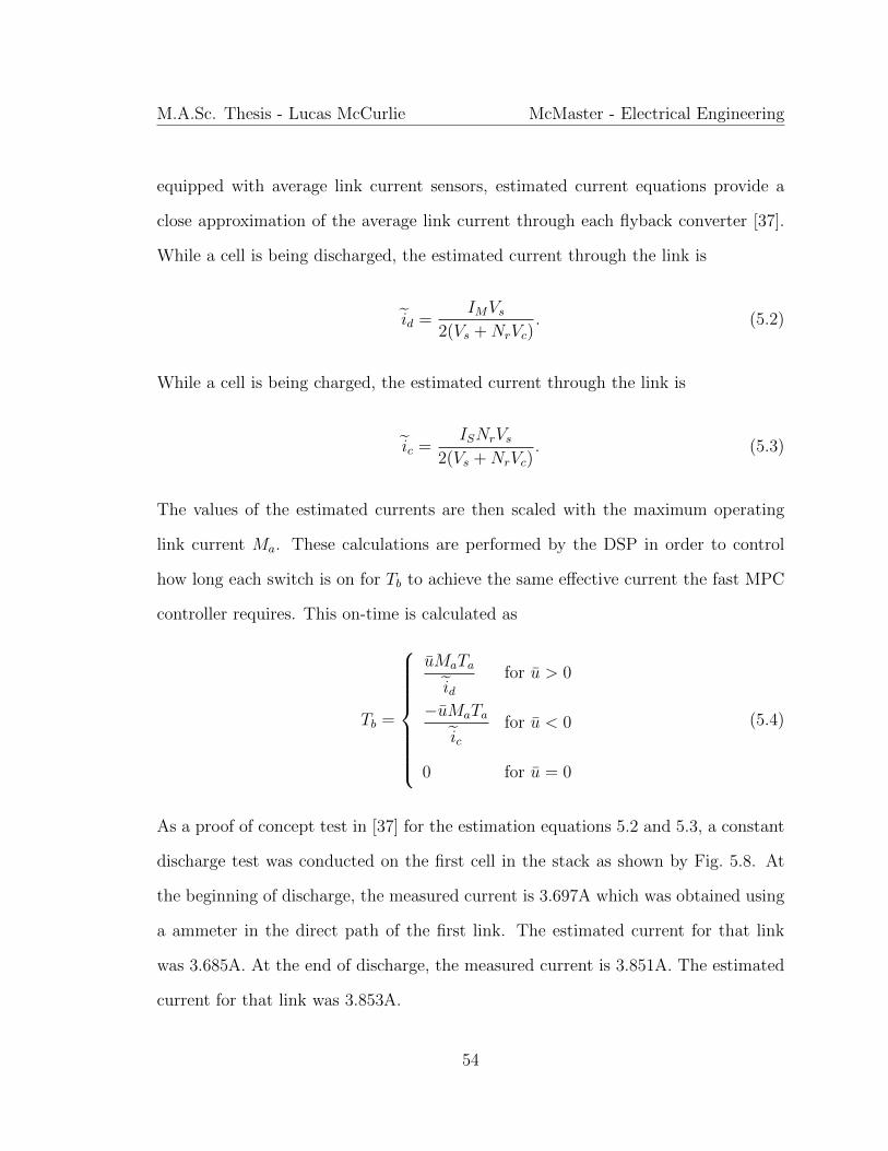
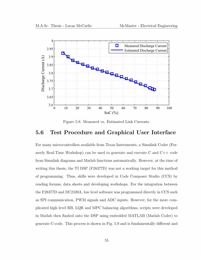
As a proof of concept test in [37] for the estimation equations 5.2 and 5.3, a constant
discharge test was conducted on the first cell in the stack as shown by Fig. 5.8. At
the beginning of discharge, the measured current is 3.697A which was obtained using
a ammeter in the direct path of the first link. The estimated current for that link
was 3.685A. At the end of discharge, the measured current is 3.851A. The estimated
current for that link was 3.853A.
54
M.A.Sc. Thesis - Lucas McCurlie McMaster - Electrical Engineering
0 10 20 30 40 50 60 70 80 90 1003.6
3.65
3.7
3.75
3.8
3.85
3.9
3.95
4
SoC (%)
Dis
char
ge C
urre
nt (
A)
Measured Discharge CurrentEstimated Discharge Current
Figure 5.8: Measured vs. Estimated Link Currents.
5.6 Test Procedure and Graphical User Interface
For many microcontrollers available from Texas Instruments, a Simulink Coder (For-
merly Real-Time Workshop) can be used to generate and execute C and C++ code
from Simulink diagrams and Matlab functions automatically. However, at the time of
writing this thesis, the TI DSP (F28377D) was not a working target for this method
of programming. Thus, skills were developed in Code Composer Studio (CCS) by
reading forums, data sheets and developing workshops. For the integration between
the F28377D and DC2100A, low level software was programmed directly in CCS such
as SPI communication, PWM signals and ADC inputs. However, for the more com-
plicated high level RB, LQR and MPC balancing algorithms, scripts were developed
in Matlab then flashed onto the DSP using embedded MATLAB (Matlab Coder) to
generate C-code. This process is shown in Fig. 5.9 and is fundamentally different and
55
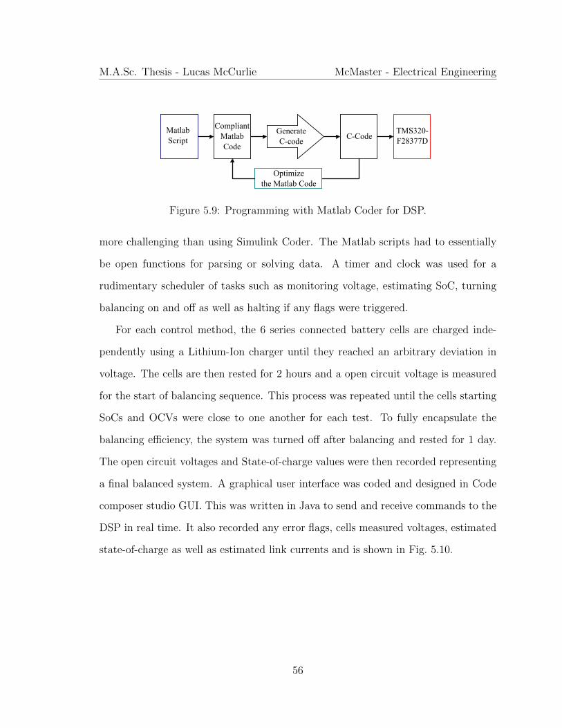
M.A.Sc. Thesis - Lucas McCurlie McMaster - Electrical Engineering
Matlab Script
CompliantMatlabCode
GenerateC-code
C-CodeTMS320-F28377D
Optimize the Matlab Code
Figure 5.9: Programming with Matlab Coder for DSP.
more challenging than using Simulink Coder. The Matlab scripts had to essentially
be open functions for parsing or solving data. A timer and clock was used for a
rudimentary scheduler of tasks such as monitoring voltage, estimating SoC, turning
balancing on and off as well as halting if any flags were triggered.
For each control method, the 6 series connected battery cells are charged inde-
pendently using a Lithium-Ion charger until they reached an arbitrary deviation in
voltage. The cells are then rested for 2 hours and a open circuit voltage is measured
for the start of balancing sequence. This process was repeated until the cells starting
SoCs and OCVs were close to one another for each test. To fully encapsulate the
balancing efficiency, the system was turned off after balancing and rested for 1 day.
The open circuit voltages and State-of-charge values were then recorded representing
a final balanced system. A graphical user interface was coded and designed in Code
composer studio GUI. This was written in Java to send and receive commands to the
DSP in real time. It also recorded any error flags, cells measured voltages, estimated
state-of-charge as well as estimated link currents and is shown in Fig. 5.10.
56
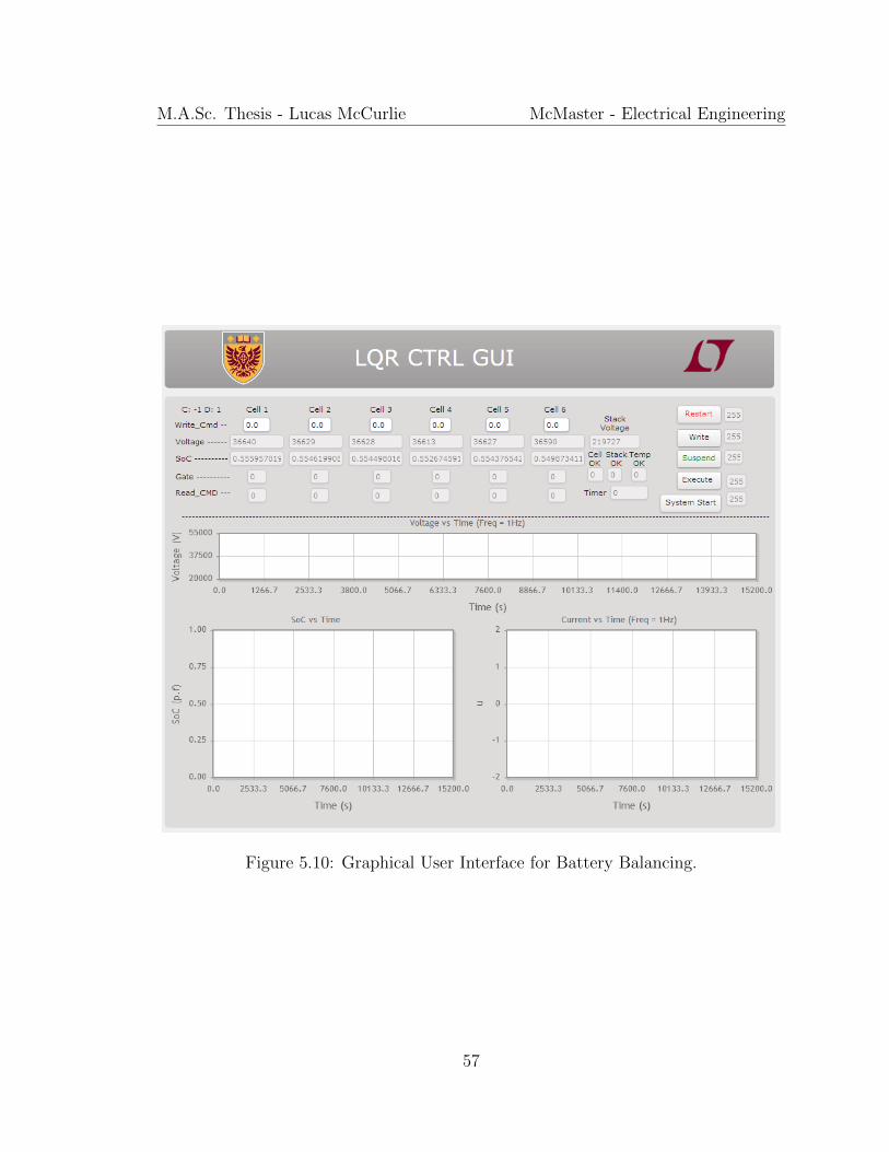
M.A.Sc. Thesis - Lucas McCurlie McMaster - Electrical Engineering
Figure 5.10: Graphical User Interface for Battery Balancing.
57
Chapter 6
Simulation results and
Experimental validation
For this thesis, different battery balancing control methods have been simulated us-
ing MATLAB. The simulation scripts for each control method can be found in the
Appendix of this Thesis. The closed loop system is compared with that of an exper-
imental one. An evaluation of the controller and balancing hardware for a system
containing 6 cells in series, each with a rated capacity of C = 6.14Ah and each link
with a maximum of I = 0.875A. The balancing hardware is carried out using flyback
converters between each cell connecting to the stack of batteries in a individual cell
to stack topology. The control methods being compared (defined earlier) are Rule
based control (RB), Linear Quadratic Regulator Control (LQR) and Model Predictive
Control (MPC). Each method has advantages and disadvantages alike and have an
associated time to balance. The linear battery model used in simulation is represented
58
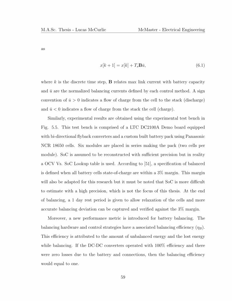
M.A.Sc. Thesis - Lucas McCurlie McMaster - Electrical Engineering
as
x[k + 1] = x[k] + TsBu, (6.1)
where k is the discrete time step, B relates max link current with battery capacity
and u are the normalized balancing currents defined by each control method. A sign
convention of u > 0 indicates a flow of charge from the cell to the stack (discharge)
and u < 0 indicates a flow of charge from the stack the cell (charge).
Similarly, experimental results are obtained using the experimental test bench in
Fig. 5.5. This test bench is comprised of a LTC DC2100A Demo board equipped
with bi-directional flyback converters and a custom built battery pack using Panasonic
NCR 18650 cells. Six modules are placed in series making the pack (two cells per
module). SoC is assumed to be reconstructed with sufficient precision but in reality
a OCV Vs. SoC Lookup table is used. According to [51], a specification of balanced
is defined when all battery cells state-of-charge are within a 3% margin. This margin
will also be adapted for this research but it must be noted that SoC is more difficult
to estimate with a high precision, which is not the focus of this thesis. At the end
of balancing, a 1 day rest period is given to allow relaxation of the cells and more
accurate balancing deviation can be captured and verified against the 3% margin.
Moreover, a new performance metric is introduced for battery balancing. The
balancing hardware and control strategies have a associated balancing efficiency (ηB).
This efficiency is attributed to the amount of unbalanced energy and the lost energy
while balancing. If the DC-DC converters operated with 100% efficiency and there
were zero losses due to the battery and connections, then the balancing efficiency
would equal to one.
59
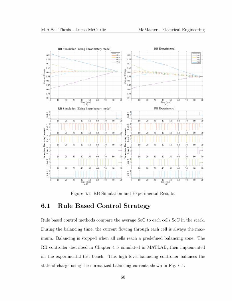
M.A.Sc. Thesis - Lucas McCurlie McMaster - Electrical Engineering
10 20 30 40 50 60 70 80 90 10 20 30 40 50 60 70 80 90
10 20 30 40 50 60 70 80 90
10 20 30 40 50 60 70 80 90
10 20 30 40 50 60 70 80 90
10 20 30 40 50 60 70 80 90
10 20 30 40 50 60 70 80 90
10 20 30 40 50 60 70 80 90
10 20 30 40 50 60 70 80 90
10 20 30 40 50 60 70 80 90
10 20 30 40 50 60 70 80 90
10 20 30 40 50 60 70 80 90
10 20 30 40 50 60 70 80 90
10 20 30 40 50 60 70 80 90
Time (min)0
Sta
te-o
f-C
harg
e
0.3
0.35
0.4
0.45
0.5
0.55
0.6
0.65
0.7
0.75
0.8
RB Simulation (Using linear battery model) RB Experimental
0
-101
-101
-101
-101
-101
-101
Nor
mal
ized
Bal
anci
ng C
urre
nts
0
0
0
0
0
0
(a.1)Time (min)
(b.1)
Time (min)(a.2)
Time (min)(b.2)
-101
-101
-101
-101
-101
-101
Nor
mal
ized
Bal
anci
ng C
urre
nts
0
0
0
0
0
0
Sta
te-o
f-C
harg
e
0.3
0.35
0.4
0.45
0.5
0.55
0.6
0.65
0.7
0.75
0.8
RB Simulation (Using linear battery model) RB Experimental
cell 1cell 2
cell 3
cell 4
cell 5cell 6
Lin
k 6
Lin
k 5
Lin
k 4
Lin
k 3
Lin
k 2
Lin
k 1
Lin
k 6
Lin
k 5
Lin
k 4
Lin
k 3
Lin
k 2
Lin
k 1
cell 1cell 2
cell 3
cell 4
cell 5cell 6
Figure 6.1: RB Simulation and Experimental Results.
6.1 Rule Based Control Strategy
Rule based control methods compare the average SoC to each cells SoC in the stack.
During the balancing time, the current flowing through each cell is always the max-
imum. Balancing is stopped when all cells reach a predefined balancing zone. The
RB controller described in Chapter 4 is simulated in MATLAB, then implemented
on the experimental test bench. This high level balancing controller balances the
state-of-charge using the normalized balancing currents shown in Fig. 6.1.
60
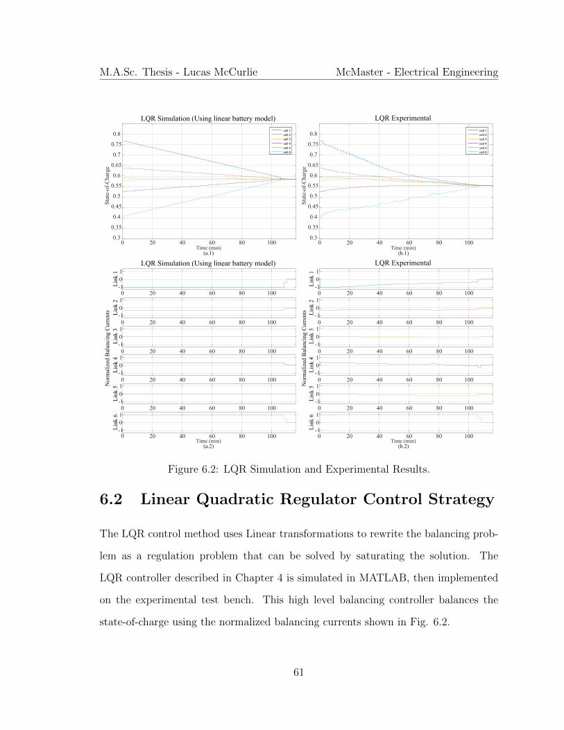
M.A.Sc. Thesis - Lucas McCurlie McMaster - Electrical Engineering
Time (min)0
Sta
te-o
f-C
harg
e
0.3
0.35
0.4
0.45
0.5
0.55
0.6
0.65
0.7
0.75
0.8
LQR Simulation (Using linear battery model) LQR Experimental
0
-101
-101
-101
-101
-101
-101
Nor
mal
ized
Bal
anci
ng C
urre
nts
0
0
0
0
0
0
(a.1)Time (min)
(b.1)
Time (min)(a.2)
Time (min)(b.2)
-101
-101
-101
-101
-101
-101
Nor
mal
ized
Bal
anci
ng C
urre
nts
0
0
0
0
0
0
Sta
te-o
f-C
harg
e
0.3
0.35
0.4
0.45
0.5
0.55
0.6
0.65
0.7
0.75
0.8
LQR Simulation (Using linear battery model) LQR Experimental
Lin
k 6
Lin
k 5
Lin
k 4
Lin
k 3
Lin
k 2
Lin
k 1
Lin
k 6
Lin
k 5
Lin
k 4
Lin
k 3
Lin
k 2
Lin
k 1
20 40 60 80 100
cell 1cell 2
cell 3
cell 4
cell 5cell 6
cell 1cell 2
cell 3
cell 4
cell 5cell 6
20 40 60 80 100
20 40 60 80 100
20 40 60 80 100
20 40 60 80 100
20 40 60 80 100
20 40 60 80 100
20 40 60 80 100
20 40 60 80 100
20 40 60 80 100
20 40 60 80 100
20 40 60 80 100
20 40 60 80 100
20 40 60 80 100
Figure 6.2: LQR Simulation and Experimental Results.
6.2 Linear Quadratic Regulator Control Strategy
The LQR control method uses Linear transformations to rewrite the balancing prob-
lem as a regulation problem that can be solved by saturating the solution. The
LQR controller described in Chapter 4 is simulated in MATLAB, then implemented
on the experimental test bench. This high level balancing controller balances the
state-of-charge using the normalized balancing currents shown in Fig. 6.2.
61
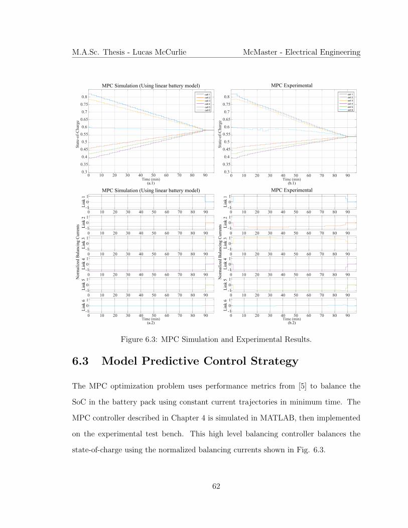
M.A.Sc. Thesis - Lucas McCurlie McMaster - Electrical Engineering
10 20 30 40 50 60 70 80 90Time (min)
0
Sta
te-o
f-C
harg
e
0.3
0.35
0.4
0.45
0.5
0.55
0.6
0.65
0.7
0.75
0.8
MPC Simulation (Using linear battery model) MPC Experimental
0
-101
-101
-101
-101
-101
-101
Nor
mal
ized
Bal
anci
ng C
urre
nts
0
0
0
0
0
0
(a.1)Time (min)
(b.1)
Time (min)(a.2)
Time (min)(b.2)
-101
-101
-101
-101
-101
-101
Nor
mal
ized
Bal
anci
ng C
urre
nts
0
0
0
0
0
0
Sta
te-o
f-C
harg
e
0.3
0.35
0.4
0.45
0.5
0.55
0.6
0.65
0.7
0.75
0.8
MPC Simulation (Using linear battery model) MPC Experimental
Lin
k 6
Lin
k 5
Lin
k 4
Lin
k 3
Lin
k 2
Lin
k 1
Lin
k 6
Lin
k 5
Lin
k 4
Lin
k 3
Lin
k 2
Lin
k 1
cell 1cell 2
cell 3
cell 4
cell 5cell 6
cell 1cell 2
cell 3
cell 4
cell 5cell 6
10 20 30 40 50 60 70 80 90
10 20 30 40 50 60 70 80 90
10 20 30 40 50 60 70 80 90
10 20 30 40 50 60 70 80 90
10 20 30 40 50 60 70 80 90
10 20 30 40 50 60 70 80 90
10 20 30 40 50 60 70 80 90
10 20 30 40 50 60 70 80 90
10 20 30 40 50 60 70 80 90
10 20 30 40 50 60 70 80 90
10 20 30 40 50 60 70 80 90
10 20 30 40 50 60 70 80 90
10 20 30 40 50 60 70 80 90
Figure 6.3: MPC Simulation and Experimental Results.
6.3 Model Predictive Control Strategy
The MPC optimization problem uses performance metrics from [5] to balance the
SoC in the battery pack using constant current trajectories in minimum time. The
MPC controller described in Chapter 4 is simulated in MATLAB, then implemented
on the experimental test bench. This high level balancing controller balances the
state-of-charge using the normalized balancing currents shown in Fig. 6.3.
62
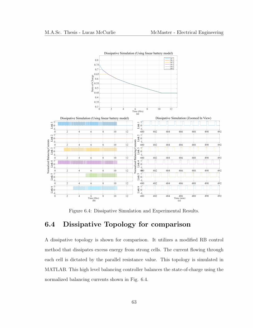
M.A.Sc. Thesis - Lucas McCurlie McMaster - Electrical Engineering
480 482 484 486 488 490 492
2 4 6 8 10 12
2 4 6 8 10 12
2 4 6 8 10 12
2 4 6 8 10 12
2 4 6 8 10 12
2 4 6 8 10 12
2 4 6 8 10 12
480 482 484 486 488 490 492
480 482 484 486 488 490 492
480 482 484 486 488 490 492
480 482 484 486 488 490 492
480 482 484 486 488 490 492
Time (Hrs)0
Sta
te-o
f-C
harg
e
0.3
0.35
0.4
0.45
0.5
0.55
0.6
0.65
0.7
0.75
0.8
Dissipative Simulation (Using linear battery model)
-101
-101
-101
-101
-101
-101
Nor
mal
ized
Bal
anci
ng C
urre
nts
0
0
0
0
0
0
(a)
Time (Hrs)(b)
Time (min)(c)
-101
-101
-101
-101
-101
-101
Nor
mal
ized
Bal
anci
ng C
urre
nts
0
Dissipative Simulation (Using linear battery model) Dissipative Simulation (Zoomed In View)
Lin
k 6
Lin
k 5
Lin
k 4
Lin
k 3
Lin
k 2
Lin
k 1
Lin
k 6
Lin
k 5
Lin
k 4
Lin
k 3
Lin
k 2
Lin
k 1
cell 1cell 2
cell 3
cell 4
cell 5cell 6
Figure 6.4: Dissipative Simulation and Experimental Results.
6.4 Dissipative Topology for comparison
A dissipative topology is shown for comparison. It utilizes a modified RB control
method that dissipates excess energy from strong cells. The current flowing through
each cell is dictated by the parallel resistance value. This topology is simulated in
MATLAB. This high level balancing controller balances the state-of-charge using the
normalized balancing currents shown in Fig. 6.4.
63
M.A.Sc. Thesis - Lucas McCurlie McMaster - Electrical Engineering
6.5 Balancing Efficiency
For a battery pack with n series connected cells with m number of links, the amount
of initial charge stored in the battery cells is Qx0 ∈ Rn. The diagonal matrix
Q =
C1 0 . . . 0
0 C2 . . . 0
......
...
0 0 . . . Cn
∈ Rnxn
defines each cells maximum charge capacities (C in Ah), and the initial state of
charge vector x0 is the amount of initial stored charge normalized by the total charge
capacity. Each element in the x0 vector ranges between zero and one where the value
of 0 corresponds to a completely empty cell and the value of 1 corresponds to a fully
charged cell. Furthermore, the matrix
V0 ∈ Rnxn,
defines another diagonal matrix containing the initial measured voltages (V) for each
cell.
A balanced point about the initial average SoC is the column vector
x0 = Jx0 ∈ Rn,
where J ∈ Rnxn is a matrix containing all 1/n elements. The difference in SoC each
64
M.A.Sc. Thesis - Lucas McCurlie McMaster - Electrical Engineering
cell is from this average is x = x0 − x0. Thus, the total initial unbalanced energy is
EU = ||Mx||1
where M = V0Q. Similarly, the final SoC vector is defined as x(τ) where τ represents
the time at which the system is balanced. Again, a diagonal matrix Vτ ∈ Rnxn defines
the final measured voltages (V) for each cell. The difference in SoC each cell is from
the initial average, xτ = x(τ) − x0, dictates how much total energy has been lost in
the system. Thus, the total energy lost is
EL = ||Mτ xτ ||1
where Mτ = VτQ.
A balancing efficiency performance metric is the overall effectiveness to redistribu-
tive the energy between the series connected cells while balancing. This metric can be
used by any balancing hardware and control implementation. It is used in this thesis
to compare the experimental results obtained in Fig. 6.1, Fig. 6.2 and Fig. 6.3. It
can be described in words as the total amount of final additional energy EA divided
by the total amount of initial unbalanced energy EU . It is now formally defined as
ηB =EAEU
=EU − ELEU
where EL is the energy lost due to balancing. Most of this loss can be attributed
to the power electronic energy conversion efficiency [15, 52, 53] and the battery cells
coulombic efficiency [10, 54], . The balancing efficiency ranges between zero and one
65
M.A.Sc. Thesis - Lucas McCurlie McMaster - Electrical Engineering
where the value of 0 corresponds to all the unbalanced energy being lost i.e dissipative
balancing and the value of 1 corresponds to perfect balancing with no losses in the
system.
6.6 Discussion
According to [51], a specification of balanced is defined when all battery cells SoC is
within a 3% margin. This thesis will try to define a more aggressive margin set of
2% difference between all SoC values. It must be noted that with a more accurate
SoC estimation strategy and low level control strategy, this value margin will decrease
substantially.
The RB experimental test started with an initial set of start-of-charge values in 6
cells as
x0 = [0.82, 0.59, 0.63, 0.42, 0.70, 0.55]
for cells 1 through 6 respectively The initial voltage set (volts) for the same corre-
sponding cells were
V0 = diag[3.9023, 3.695, 3.7294, 3.5712, 3.7968, 3.6595]
The test originally started with an arbitrary unbalance of 40% difference in maximum
and minimum SoC and 331mV in starting voltages. At the end of balancing and
after the predefined rest period, this system had a ending set of start-of-charge values
equivalent to
xτ = [0.56, 0.55, 0.56, 0.54, 0.56, 0.55]
66

M.A.Sc. Thesis - Lucas McCurlie McMaster - Electrical Engineering
Sta
te-o
f-C
harg
e
0.3
0.4
0.5
0.6
0.7
0.8
0.9
1
0.2
0.1
0
RB Unbalanced SoC
Cell 1 Cell 2 Cell 3 Cell 4 Cell 5 Cell 6(a)
Sta
te-o
f-C
harg
e
0.3
0.4
0.5
0.6
0.7
0.8
0.9
1
0.2
0.1
0
RB balanced SoC
Cell 1 Cell 2 Cell 3 Cell 4 Cell 5 Cell 6(b)
Figure 6.5: RB Unbalanced(a); Balanced(b) State-of-Charge.
The final voltage set in volts was
V0 = diag[3.6703, 3.6581, 3.6645, 3.6514, 3.6691, 3.6610]
This shows the test ended with just a 2% difference in maximum and minimum SoC
was achieved with 18.9mV difference in final voltages. According to the balance
margin, RB was able to successfully balance the cells state-of-charge. However, the
balancing efficiency for the RB method was calculated to be 0.36, due to the lost
energy of the intermediate cells being charge and discharged until the end.
For the LQR experimental test, an initial set of start-of-charge values was
x0 = [0.77, 0.64, 0.58, 0.52, 0.60, 0.41]
67
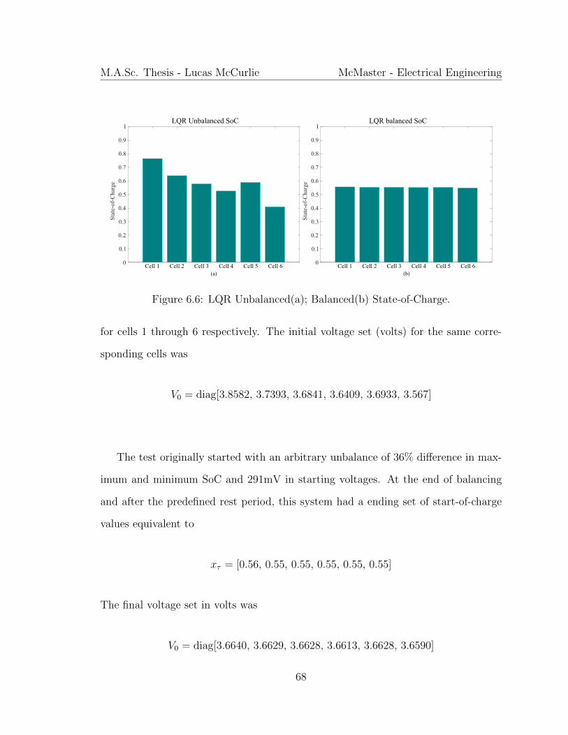
M.A.Sc. Thesis - Lucas McCurlie McMaster - Electrical Engineering
Sta
te-o
f-C
harg
e
0.3
0.4
0.5
0.6
0.7
0.8
0.9
1
0.2
0.1
0
LQR Unbalanced SoC
Cell 1 Cell 2 Cell 3 Cell 4 Cell 5 Cell 6(a)
Sta
te-o
f-C
harg
e
0.3
0.4
0.5
0.6
0.7
0.8
0.9
1
0.2
0.1
0
LQR balanced SoC
Cell 1 Cell 2 Cell 3 Cell 4 Cell 5 Cell 6(b)
Figure 6.6: LQR Unbalanced(a); Balanced(b) State-of-Charge.
for cells 1 through 6 respectively. The initial voltage set (volts) for the same corre-
sponding cells was
V0 = diag[3.8582, 3.7393, 3.6841, 3.6409, 3.6933, 3.567]
The test originally started with an arbitrary unbalance of 36% difference in max-
imum and minimum SoC and 291mV in starting voltages. At the end of balancing
and after the predefined rest period, this system had a ending set of start-of-charge
values equivalent to
xτ = [0.56, 0.55, 0.55, 0.55, 0.55, 0.55]
The final voltage set in volts was
V0 = diag[3.6640, 3.6629, 3.6628, 3.6613, 3.6628, 3.6590]
68
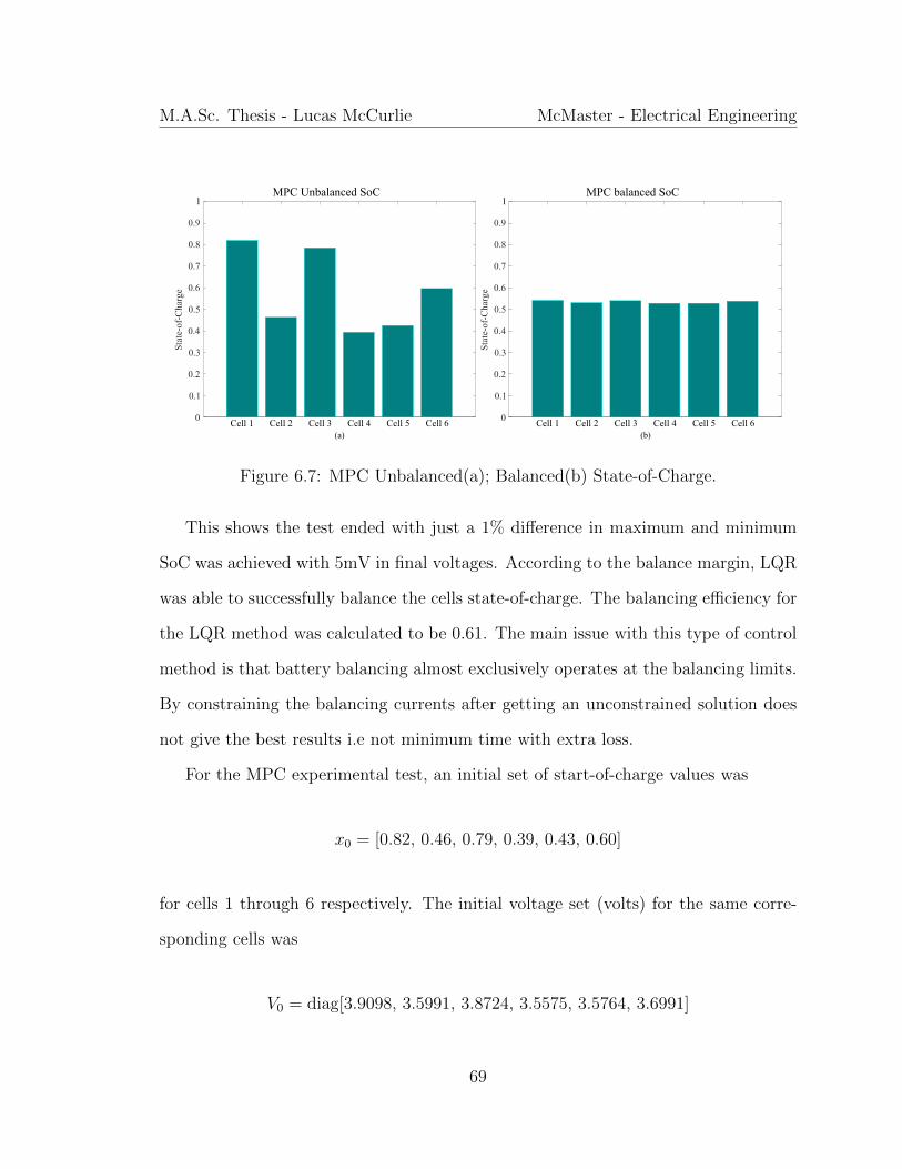
M.A.Sc. Thesis - Lucas McCurlie McMaster - Electrical Engineering
Sta
te-o
f-C
harg
e
0.3
0.4
0.5
0.6
0.7
0.8
0.9
1
0.2
0.1
0
MPC Unbalanced SoC
Cell 1 Cell 2 Cell 3 Cell 4 Cell 5 Cell 6(a)
Sta
te-o
f-C
harg
e
0.3
0.4
0.5
0.6
0.7
0.8
0.9
1
0.2
0.1
0
MPC balanced SoC
Cell 1 Cell 2 Cell 3 Cell 4 Cell 5 Cell 6(b)
Figure 6.7: MPC Unbalanced(a); Balanced(b) State-of-Charge.
This shows the test ended with just a 1% difference in maximum and minimum
SoC was achieved with 5mV in final voltages. According to the balance margin, LQR
was able to successfully balance the cells state-of-charge. The balancing efficiency for
the LQR method was calculated to be 0.61. The main issue with this type of control
method is that battery balancing almost exclusively operates at the balancing limits.
By constraining the balancing currents after getting an unconstrained solution does
not give the best results i.e not minimum time with extra loss.
For the MPC experimental test, an initial set of start-of-charge values was
x0 = [0.82, 0.46, 0.79, 0.39, 0.43, 0.60]
for cells 1 through 6 respectively. The initial voltage set (volts) for the same corre-
sponding cells was
V0 = diag[3.9098, 3.5991, 3.8724, 3.5575, 3.5764, 3.6991]
69
M.A.Sc. Thesis - Lucas McCurlie McMaster - Electrical Engineering
The test originally started with an arbitrary unbalance of 43% difference in maximum
and minimum SoC and 351mV in starting voltages. At the end of balancing and
after the predefined rest period, this system had a ending set of start-of-charge values
equivalent to
xτ = [0.54, 0.53, 0.54, 0.53, 0.53, 0.54]
The final voltage set in volts was
V0 = diag[3.6531, 3.6447, 3.6520, 3.6434, 3.6432, 3.6509]
This shows the test ended with just a 1% difference in maximum and minimum SoC
was achieved with 9mV in final voltages. According to the balance margin, MPC
was able to successfully balance the cells state-of-charge. The balancing efficiency
for the MPC method was calculated to be the highest out of the three controllers at
0.71. This is because the intermediate cells have more constant current trajectories
and is balanced in the minimum time as both the strongest and weakest cells are
operated with the maximum link currents. A final remark about these results is that
this shows a clear motivation behind adopting a MPC approach which is to apply
more of a constant current that results in higher balancing efficiency and minimum
time to balance.
70
Chapter 7
Conclusions
Many cells in a pack configured in both series and parallel orientations introduce
monitoring and management difficulties. The capacity and the lifetime of the battery
pack are determined by the weakest cell. Each cell must be properly monitored to
prevent overcharge and over discharge of Lithium-ion cells. The differences in state-of-
charge will cause further variations between each cell that only grow with time. To use
the entire effective pack capacity, balancing the individual cells needs to occur. This
thesis shows varies balancing topologies found in literature and implements a multiple
transformer individual cell to stack topology for redistributive non-dissipative battery
balancing. This was the chosen topology because in [5], the time to balance and energy
dissipated remained constant as the number of cells increased.
Furthermore, three high level control strategies were designed to balance, i.e.
equalize the state-of-charge of n number of series connected cells with m links. The
control methods are rule based (RB) control, Linear Quadratic Regulator (LQR)
control and Model Predictive Control (MPC). For comparison, a typical active dis-
sipated topology using switched resistors [19, 38] was used with a rule based control
71
M.A.Sc. Thesis - Lucas McCurlie McMaster - Electrical Engineering
that drives the higher SoCs to the minimum SoC. If resistor values are chosen such
that the current is small or less than 10mA/Ahr capacity, then each cell roughly can
balance at a rate of 1% per hour [38]. However, if trying to employ the redistribu-
tive technique i.e operating all the time not just during charging then this technique
could drain the entire battery pack in a few days [38]. Furthermore, it has a balancing
efficiency of zero because the total initial unbalanced energy is lost i.e EU = EL.
The high level controllers are based on a general battery pack model that can be
adopted for cells with different capacities since each cell is modeled by its capacity and
state-of-charge. Also, it can be combined with various battery balancing topologies
that are modeled by a topology matrix defined in [5] and the maximum current in
each link. In practice, isolated DC/DC converters actuate the average balancing
current defined by the high level controller. For the high level LQR controller, Linear
transformations are used to transform the control into a regulation problem and to
ensure that the control input is feasible. The main issue with this type of control
method is that battery balancing almost exclusively operates at the balancing limits.
By constraining the balancing currents after getting an unconstrained solution does
not give the best results i.e not minimum time with extra loss. This result is validated
by having a worse balancing efficiency than MPC of 0.61. The fast MPC controller
is developed based on the minimum time to balance performance metric in [5]. The
fast MPC controller applies the maximum input u if τ > Ts. If τ ≤ Ts then the input
is scaled by a τTs
factor. The MPC approach is compared to a rule based strategy
and shows that constant current will result in a single point of converge of the SoCs.
This reduces any micro-cycles between charging and discharging of the intermediate
battery cells [55] and improves the balancing efficiency.
72

Appendix
73
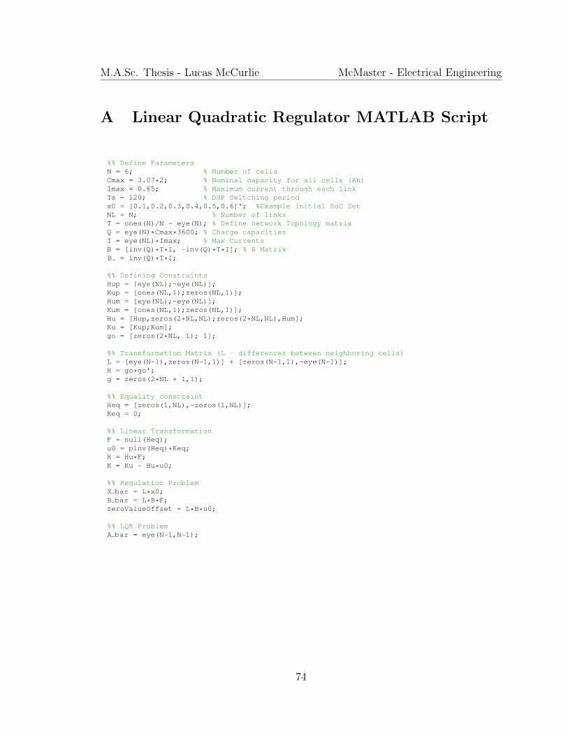
M.A.Sc. Thesis - Lucas McCurlie McMaster - Electrical Engineering
A Linear Quadratic Regulator MATLAB Script
%% Define ParametersN = 6; % Number of cellsCmax = 3.07*2; % Nominal capacity for all cells (Ah)Imax = 0.85; % Maximum current through each linkTs = 120; % DSP Switching periodx0 = [0.1,0.2,0.3,0.4,0.5,0.6]'; %Example initial SoC SetNL = N; % Number of linksT = ones(N)/N - eye(N); % Define network Topology matrixQ = eye(N)*Cmax*3600; % Charge capacitiesI = eye(NL)*Imax; % Max CurrentsB = [inv(Q)*T*I, -inv(Q)*T*I]; % B MatrixB = inv(Q)*T*I;
%% Defining ConstraintsHup = [eye(NL);-eye(NL)];Kup = [ones(NL,1);zeros(NL,1)];Hum = [eye(NL);-eye(NL)];Kum = [ones(NL,1);zeros(NL,1)];Hu = [Hup,zeros(2*NL,NL);zeros(2*NL,NL),Hum];Ku = [Kup;Kum];go = [zeros(2*NL, 1); 1];
%% Transformation Matrix (L - differences between neighboring cells)L = [eye(N-1),zeros(N-1,1)] + [zeros(N-1,1),-eye(N-1)];H = go*go';g = zeros(2*NL + 1,1);
%% Equality constraintHeq = [zeros(1,NL),-zeros(1,NL)];Keq = 0;
%% Linear TransformationF = null(Heq);u0 = pinv(Heq)*Keq;H = Hu*F;K = Ku - Hu*u0;
%% Regulation ProblemX bar = L*x0;B bar = L*B*F;zeroValueOffset = L*B*u0;
%% LQR ProblemA bar = eye(N-1,N-1);
1
74
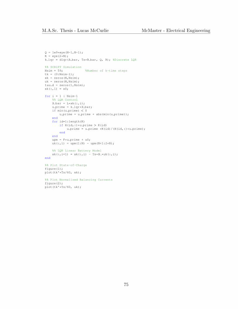
M.A.Sc. Thesis - Lucas McCurlie McMaster - Electrical Engineering
Q = 1e9*eye(N-1,N-1);R = eye(2*N);k lqr = dlqr(A bar, Ts*B bar, Q, R); %Discrete LQR
%% SCRIPT SimulationNsim = 59; %Number of k-time stepstk = (0:Nsim-1);xk = zeros(N,Nsim);uk = zeros(N,Nsim);tau d = zeros(1,Nsim);xk(:,1) = x0;
for i = 1 : Nsim-1%% LQR ControlX bar = L*xk(:,i);u prime = k lqr*X bar;if min(u prime) < 0
u prime = u prime + abs(min(u prime));endfor id=1:length(K)
if H(id,:)*u prime > K(id)u prime = u prime *K(id)/(H(id,:)*u prime);
endendupm = F*u prime + u0;uk(:,i) = upm(1:N) - upm(N+1:2*N);
%% LQR Linear Battery Modelxk(:,i+1) = xk(:,i) - Ts*B *uk(:,i);
end
%% Plot State-of-Chargefigure(1);plot(tk'*Ts/60, xk);
%% Plot Normalized Balancing Currentsfigure(2);plot(tk'*Ts/60, uk);
2
75
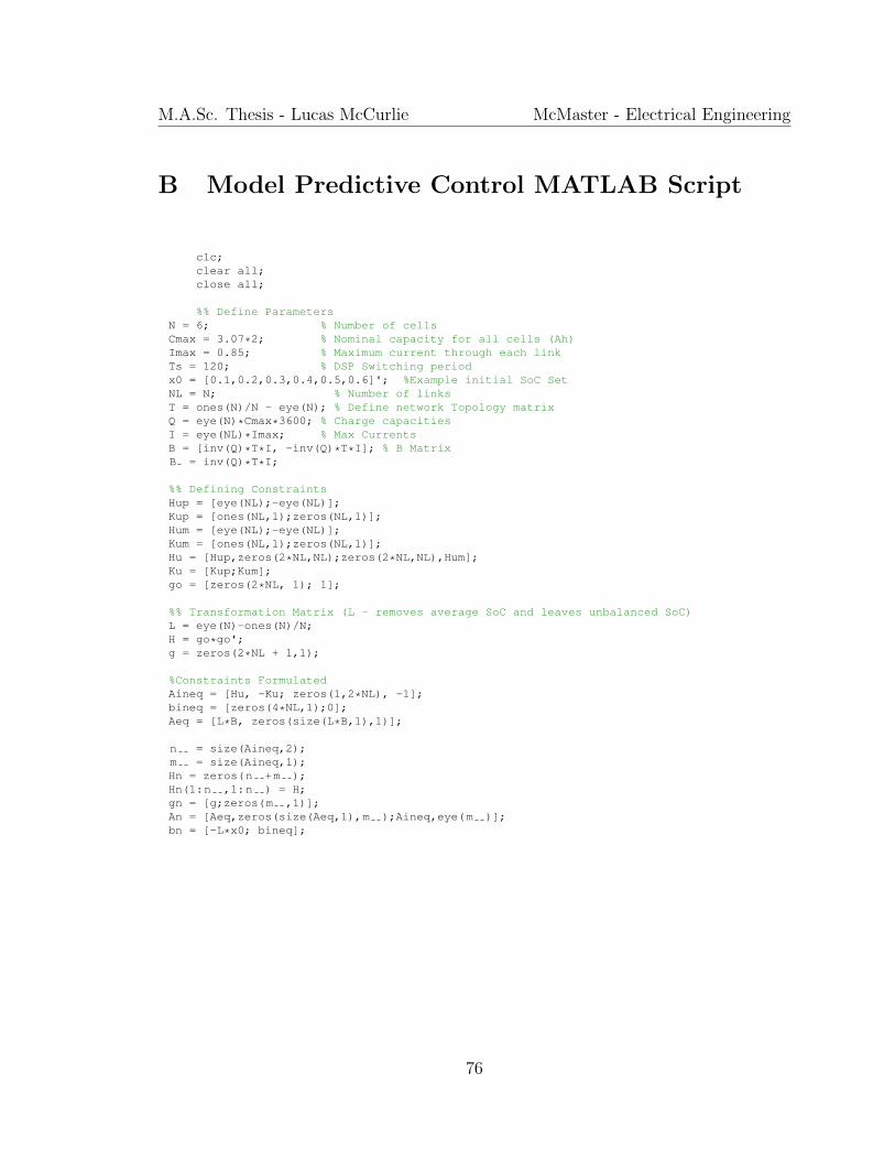
M.A.Sc. Thesis - Lucas McCurlie McMaster - Electrical Engineering
B Model Predictive Control MATLAB Script
clc;clear all;close all;
%% Define ParametersN = 6; % Number of cellsCmax = 3.07*2; % Nominal capacity for all cells (Ah)Imax = 0.85; % Maximum current through each linkTs = 120; % DSP Switching periodx0 = [0.1,0.2,0.3,0.4,0.5,0.6]'; %Example initial SoC SetNL = N; % Number of linksT = ones(N)/N - eye(N); % Define network Topology matrixQ = eye(N)*Cmax*3600; % Charge capacitiesI = eye(NL)*Imax; % Max CurrentsB = [inv(Q)*T*I, -inv(Q)*T*I]; % B MatrixB = inv(Q)*T*I;
%% Defining ConstraintsHup = [eye(NL);-eye(NL)];Kup = [ones(NL,1);zeros(NL,1)];Hum = [eye(NL);-eye(NL)];Kum = [ones(NL,1);zeros(NL,1)];Hu = [Hup,zeros(2*NL,NL);zeros(2*NL,NL),Hum];Ku = [Kup;Kum];go = [zeros(2*NL, 1); 1];
%% Transformation Matrix (L - removes average SoC and leaves unbalanced SoC)L = eye(N)-ones(N)/N;H = go*go';g = zeros(2*NL + 1,1);
%Constraints FormulatedAineq = [Hu, -Ku; zeros(1,2*NL), -1];bineq = [zeros(4*NL,1);0];Aeq = [L*B, zeros(size(L*B,1),1)];
n = size(Aineq,2);m = size(Aineq,1);Hn = zeros(n +m );Hn(1:n ,1:n ) = H;gn = [g;zeros(m ,1)];An = [Aeq,zeros(size(Aeq,1),m );Aineq,eye(m )];bn = [-L*x0; bineq];
1
76
M.A.Sc. Thesis - Lucas McCurlie McMaster - Electrical Engineering
%% SCRIPT SimulationNsim = 59; %Number of k-time stepstk = (0:Nsim-1);xk = zeros(N,Nsim);uk = zeros(N,Nsim);tau d = zeros(1,Nsim);xk(:,1) = x0;
for i = 1 : Nsim-1%% MPC Controlbn = [-L*xk(:,i); bineq];% Substitute MPC SOLVER with stnd solvers such as CPLEX & qpOASES[x micro, exitflag] = MPC SOLVER(Hn, gn, An, bn);
%% Post Process x microtau = max(x micro(2*N+1),1e-12);vpm = x micro(1:2*N);if tau > Ts
upm out = vpm/tau ;else
if tau > 0upm out = vpm/Ts;
elseupm out = zeros(2*6,1);
endendu = (upm out(1:N) -upm out(N+1:2*N));
%% MPC Linear Battery Modelxk(:,i+1) = xk(:,i) + Ts*B *uk(:,i);
end
%% Plot State-of-Chargefigure(1);plot(tk'*Ts/60, xk);
%% Plot Normalized Balancing Currentsfigure(2);plot(tk'*Ts/60, uk);
2
77

M.A.Sc. Thesis - Lucas McCurlie McMaster - Electrical Engineering
C Rule Based MATLAB Script
clc;clear all;close all;
%% Define ParametersN = 6; % Number of cellsCmax = 3.07*2; % Nominal capacity for all cells (Ah)Imax = 0.85; % Maximum current through each linkTs = 120; % DSP Switching periodx0 = [0.1,0.2,0.3,0.4,0.5,0.6]'; %Example initial SoC SetNL = N; % Number of linksT = ones(N)/N - eye(N); % Define network Topology matrixQ = eye(N)*Cmax*3600; % Charge capacitiesI = eye(NL)*Imax; % Max CurrentsB = [inv(Q)*T*I, -inv(Q)*T*I]; % B MatrixB = inv(Q)*T*I;L = eye(N)-ones(N)/N;
%% SCRIPT SimulationNsim = 59; %Number of k-time stepstk = (0:Nsim-1);xk = zeros(N,Nsim);uk = zeros(N,Nsim);tau d = zeros(1,Nsim);xk(:,1) = x0;
for i = 1 : Nsim-1%% Rule based controlsoc average = sum(xk(:,i))/N;tdL = norm(L*xk(:,i),1);for iL = 1:N
if(tdL > 0.005)if (xk(iL,i) >= soc average )
% If above average, discharge.upm1(iL) = 1;upm2(iL) = 0;
elseif (xk(iL,i) < soc average )% If below average, charge.upm1(iL) = 0;upm2(iL) = -1;
endenduk(iL,i) = upm1(iL) + upm2(iL);
end
1
78
M.A.Sc. Thesis - Lucas McCurlie McMaster - Electrical Engineering
% Linear Plant Modelxk(:,i+1) = xk(:,i) + Ts*B *uk(:,i);
end
%% Plot State-of-Chargefigure(1);plot(tk'*Ts/60, xk);
%% Plot Normalized Balancing Currentsfigure(2);plot(tk'*Ts/60, uk);
2
79
Bibliography
[1] B. Bilgin, P. Magne, P. Malysz, Y. Yang, V. Pantelic, M. Preindl, A. Korobkine,
W. Jiang, M. Lawford, and A. Emadi, “Making the Case for Electrified Trans-
portation,” IEEE Transactions on Transportation Electrification, vol. 1, no. 1,
pp. 4–17, 2015.
[2] The Boston Consulting Group, “Batteries for Electric Cars - Challenges, Oppor-
tunities, and the Outlook to 2020,” Tech. Rep. 1, 2010.
[3] Panasonic, “Panasonic NCR18650A Datasheet,” Tech. Rep., 2012.
[4] D. Andrea, Battery Management Systems for Large Lithium-ion Battery Packs.
Artech House, 2010.
[5] M. Preindl, C. Danielson, and F. Borrelli, “Performance evaluation of battery
balancing hardware,” in European Control Conference, jul 2013, pp. 4065–4070.
[6] A. Saliva, “Design Guide for Off-line Fixed Frequency DCM Flyback Converter,”
Infineon, Tech. Rep. January, 2013.
[7] LTC, “Linear Technology - LTC DC2100A Demoboard: User Manual,” Tech.
Rep., 2013.
80

M.A.Sc. Thesis - Lucas McCurlie McMaster - Electrical Engineering
[8] ——, “Linear Technology - LTC3300-1: High Efficiency Bidirectional Multicell
Battery Balancer (Datasheet),” Tech. Rep., 2013.
[9] International Technology Perspectives 2008 - Scenarios and strategies to 2050.
International Energy Agency, 2008.
[10] E. Chemali, M. Peindl, P. Malysz, and A. Emadi, “Electrochemical and Elec-
trostatic Energy Storage and Management Systems for Electric Drive Vehicles:
State-of-the-Art Review and Future Trends,” IEEE Journal of Emerging and
Selected Topics in Power Electronics, vol. 6777, no. c, pp. 1–1, 2016.
[11] N. Rauh, T. Franke, and J. F. Krems, “Understanding the Impact of Electric
Vehicle Driving Experience on Range Anxiety,” Human Factors: The Journal of
the Human Factors and Ergonomics Society, vol. 57, no. 1, pp. 177–187, 2015.
[12] O. Veneri, L. Ferraro, C. Capasso, and D. Iannuzzi, “Charging infrastructures
for EV: Overview of technologies and issues,” Electrical Systems for Aircraft,
Railway and Ship Propulsion, ESARS, pp. 0–5, 2012.
[13] California Environmental Protection Agency Air Resources Board, “Technology
Assessment: Medium- and Heavy- Duty Battery Electric Trucks and Buses,”
Tech. Rep. October 2015 (Draft), 2015.
[14] S. Abu-Sharkh and D. Doerffel, “Rapid test and non-linear model characterisa-
tion of solid-state lithium-ion batteries,” Journal of Power Sources, vol. 130, no.
1-2, pp. 266–274, 2004.
81
M.A.Sc. Thesis - Lucas McCurlie McMaster - Electrical Engineering
[15] N. H. Kutkut, H. L. N. Wiegman, D. M. Divan, and D. W. Novotny, “Charge
equalization for an electric vehicle battery system,” IEEE Transactions on
Aerospace and Electronic Systems, vol. 34, no. 1, pp. 235–246, 1998.
[16] B. Lindemark, “Individual cell voltage equalizers (ICE) for reliable battery per-
formance,” in Energy Conference, vol. 91, 1991, pp. 196–201.
[17] C. S. Moo, Y. C. Hsieh, and I. S. Tsai, “Charge equalization for series-connected
batteries,” IEEE Transactions on Aerospace and Electronic Systems, vol. 39,
no. 2, pp. 704–710, 2003.
[18] N. H. Kutkut and D. M. Divan, “Dynamic equalization techniques for series
battery stacks,” in International Telecommunications Energy Conference, 1996,
pp. 514–521.
[19] J. Cao, N. Schofield, and A. Emadi, “Battery balancing methods: A compre-
hensive review,” in IEEE Vehicle Power and Propulsion Conference, 2008, pp.
3–8.
[20] R. Lache, D. Galves, and P. Nolan, “Electric cars: Plugged in 2,” Tech. Rep.
November, 2009.
[21] D. H. Zhang, S. Qiu, G. R. Zhu, and W. Chen, “Balancing Control Strategy
for Li-ion Batteries String Based on Dynamic Balanced Point,” in IEEE Vehicle
Power and Propulsion Conference, no. 2011, 2013, pp. 60–64.
82
M.A.Sc. Thesis - Lucas McCurlie McMaster - Electrical Engineering
[22] N. Omar, M. Daowd, P. van den Bossche, O. Hegazy, J. Smekens, T. Coosemans,
and J. van Mierlo, “Rechargeable energy storage systems for plug-in hybrid elec-
tric vehicles-assessment of electrical characteristics,” Energies, vol. 5, no. 8, pp.
2952–2988, 2012.
[23] McMaster University, “MechEng739: Management and Control of Electric Ve-
hicle Batteries,” 2015.
[24] B. Xiao and Y. Shi, “A universal state-of-charge algorithm for batteries,” in
Design Automation Conference, 2010, pp. 687–692.
[25] G. L. Plett, “Extended Kalman filtering for battery management systems of
LiPB-based HEV battery packs. Part 1: Background,” Journal of Power Sources,
vol. 161, no. 2, pp. 1356–1368, 2004.
[26] M. Charkhgard and M. Farrokhi, “State-of-charge estimation for lithium-ion
batteries using neural networks and EKF,” IEEE Transactions on Industrial
Electronics, vol. 57, no. 12, pp. 4178–4187, 2010.
[27] D. Howey, P. Mitcheson, V. Yufit, G. Offer, and N. Brandon, “Online measure-
ment of battery impedance using motor controller excitation,” IEEE Transac-
tions on Vehicular Technology, vol. 63, no. 6, pp. 2557–2566, 2014.
[28] R. Feng, S. Zhao, and X. Lu, “On-line estimation of Dynamic State-of-Charge
for lead acid battery based on fuzzy logic,” in International Conference on Mea-
surement, Information and Control, no. 1, 2013, pp. 447–451.
83
M.A.Sc. Thesis - Lucas McCurlie McMaster - Electrical Engineering
[29] R. Ling, Y. Dong, H. Yan, M. Wu, and Y. Chai, “Fuzzy-PI control battery
equalization for series connected lithium-ion battery strings,” in Electronics and
Motion Control Conference (IPEMC), vol. 4, no. 5, 2012, pp. 2631–2635.
[30] K. Young, C. Wang, L. Y. Wang, and K. Strunz, Electric Vehicle Integration
into Modern Power Networks, 2013.
[31] S. M. Lukic, J. Cao, R. C. Bansal, F. Rodriguez, and A. Emadi, “Energy storage
systems for automotive applications,” IEEE Transactions on Industrial Electron-
ics, vol. 55, no. 6, pp. 2258–2267, 2008.
[32] A. Affanni, A. Bellini, G. Franceschini, P. Guglielmi, and C. Tassoni, “Battery
choice and management for new-generation electric vehicles,” IEEE Transactions
on Industrial Electronics, vol. 52, no. 5, pp. 1343–1349, 2005.
[33] M. J. Isaacson, R. P. Hollandsworth, P. J. Giampaoli, F. A. Linkowsky, A. Salim,
and V. L. Teofil, “Advanced Lithium Ion Battery Charger,” in Fifteenth Annu.
Battery Conf. Applications and Advances, 2000, pp. 798–801.
[34] G. Mulder, N. Omar, S. Pauwels, M. Meeus, F. Leemans, B. Verbrugge, W. De
Nijs, P. Van Den Bossche, D. Six, and J. Van Mierlo, “Comparison of commercial
battery cells in relation to material properties,” Electrochimica Acta, vol. 87, pp.
473–488, 2013.
[35] H. Popp, J. Attia, F. Delcorso, and A. Trifonova, “Lifetime analysis of four
different lithium ion batteries for ( plugin ) electric vehicle,” Transport Research
Arena, 2014.
84
M.A.Sc. Thesis - Lucas McCurlie McMaster - Electrical Engineering
[36] H. Chen, T. N. Cong, W. Yang, C. Tan, Y. Li, and Y. Ding, “Progress in electrical
energy storage system: A critical review,” Progress in Natural Science, vol. 19,
no. 3, pp. 291–312, 2009.
[37] L. Mccurlie, M. Preindl, P. Malysz, and A. Emadi, “Simplified Control for Redis-
tributive Balancing Systems using Bidirectional Flyback Converters,” in IEEE
Transportation Electrification Conference and Exposition, 2015.
[38] S. Moore and P. Schneider, “A Review of Cell Equalization Methods for Lithium
Ion and Lithium Polymer Battery Systems,” SAE World Congress, pp. Doc.
2001–01–0959, 2001.
[39] B. Lawson, “A Software Configurable Battery,” EVS26 International Battery,
Hybrid and Fuel Cell Electric Vehicle Symposium, Los Angeles, California, 2012.
[40] N. H. Kutkut, “A Modular Non Dissipative Current Diverter For Ev Battery
Charge Equalization,” in Applied Power Electronics Conference and Exposition,
1998, pp. 686–690.
[41] M. Daowd, N. Omar, P. van den Bossche, and J. van Mierlo, “A review of pas-
sive and active battery balancing based on MATLAB/Simulink,” International
Review of Electrical Engineering, vol. 6, no. 7, pp. 2974–2989, 2011.
[42] R. Erickson, “The Flyback Converter - Lecture notes ECEN4517,” 2012.
[43] Y. Barksukov and J. Qian, Battery Power Management for Portable Devices,
2013.
85

M.A.Sc. Thesis - Lucas McCurlie McMaster - Electrical Engineering
[44] M. Caspar and S. Hohmann, “Optimal Cell Balancing with Model-based Cascade
Control by Duty Cycle Adaption,” The International Federation of Automatic
Control, pp. 10 311–10 318, 2014.
[45] E. D. Sontag, “An algebraic approach to bounded controllability of linear sys-
tems,” International Journal of Control, vol. 39, no. 1, pp. 181–188, 1984.
[46] J. Choi, “On the stabilization of linear discrete time systems subject to input
saturation,” Systems & Control Letters, vol. 36, 1999.
[47] T. Hofman, M. Steinbuch, R. M. V. Druten, and a. F. a. Serrarens, “Rule-
Based Equivalent Fuel Consumption Minimization Strategies for Hybrid Vehi-
cles,” IFAC Symposium on Mechatronic Systems, vol. 17, no. 1, 2008.
[48] S. Malkhandi, “Fuzzy logic-based learning system and estimation of state-of-
charge of lead-acid battery,” Engineering Applications of Artificial Intelligence,
vol. 19, no. 5, pp. 479–485, 2006.
[49] M. Sorrentino, G. Rizzo, and I. Arsie, “Analysis of a rule-based control strategy
for on-board energy management of series hybrid vehicles,” Control Engineering
Practice, vol. 19, no. 12, pp. 1433–1441, 2011.
[50] LTC, “Linear Technology - DC2100A: Bi-Directional Cell Balancer,” Tech. Rep.
[51] A. M. Imtiaz and F. H. Khan, “”Time shared flyback converter” based regener-
ative cell balancing technique for series connected li-ion battery strings,” IEEE
Transactions on Power Electronics, vol. 28, no. 12, pp. 5960–5975, 2013.
[52] S. A. Akbarabadi, H. Atighechi, and J. Jatskevich, “Corrected state-space
averaged-value modeling of second-order flyback converter including conduction
86
M.A.Sc. Thesis - Lucas McCurlie McMaster - Electrical Engineering
losses,” in IEEE Canadian Conference of Electrical and Computer Engineering,
2013.
[53] Y. Yuanmao, K. W. E. Cheng, and Y. P. B. Yeung, “Zero-current switching
switched-capacitor zero-voltage-gap automatic equalization system for series bat-
tery string,” IEEE Transactions on Power Electronics, vol. 27, no. 7, pp. 3234–
3242, 2012.
[54] H. He, R. Xiong, and J. Fan, “Evaluation of Lithium-Ion Battery Equivalent
Circuit Models for State of Charge Estimation by an Experimental Approach,”
Energies, vol. 4, no. 12, pp. 582–598, 2011.
[55] E. Chemali, L. Mccurlie, B. Howey, T. Stiene, M. M. Rahman, M. Preindl,
R. Ahmed, and A. Emadi, “Minimizing Battery Wear in a Battery-Ultracapacitor
Hybrid Energy Storage System using a Linear Quadratic Regulator,” in IEEE
IECON, 2015, pp. 3265–3270.
87