IZA DP No. 1057

Redesigning Teams and Incentives in a Merger:An Experiment with Managers and Students

Claude MontmarquetteJean-Louis RullièreMarie-Claire VillevalRomain Zeiliger

DI

SC

US

SI

ON

PA

PE

R S

ER

IE

S

Forschungsinstitutzur Zukunft der ArbeitInstitute for the Studyof Labor

March 2004

Redesigning Teams and Incentives in a Merger: An Experiment with

Managers and Students

Claude Montmarquette CIRANO and University of Montreal

Jean-Louis Rullière

GATE, CNRS and University of Lumiere Lyon 2

Marie-Claire Villeval GATE, CNRS, University of Lumiere Lyon 2

and IZA Bonn

Romain Zeiliger GATE, CNRS, and University of Lumiere Lyon 2

Discussion Paper No. 1057 March 2004

IZA

P.O. Box 7240 53072 Bonn

Germany

Phone: +49-228-3894-0 Fax: +49-228-3894-180

Email: iza@iza.org

Any opinions expressed here are those of the author(s) and not those of the institute. Research disseminated by IZA may include views on policy, but the institute itself takes no institutional policy positions. The Institute for the Study of Labor (IZA) in Bonn is a local and virtual international research center and a place of communication between science, politics and business. IZA is an independent nonprofit company supported by Deutsche Post World Net. The center is associated with the University of Bonn and offers a stimulating research environment through its research networks, research support, and visitors and doctoral programs. IZA engages in (i) original and internationally competitive research in all fields of labor economics, (ii) development of policy concepts, and (iii) dissemination of research results and concepts to the interested public. IZA Discussion Papers often represent preliminary work and are circulated to encourage discussion. Citation of such a paper should account for its provisional character. A revised version may be available on the IZA website (www.iza.org) or directly from the author.

IZA Discussion Paper No. 1057 March 2004

ABSTRACT

Redesigning Teams and Incentives in a Merger: An Experiment with Managers and Students∗

After a merger, company officials face the challenge of making compensation schemes uniform and of redesigning teams with managers from companies with different incentives, work habits and recruiting methods. In this paper, we investigate the relationship between executive pay and performance after a merger by dissociating the respective influence of shifts, which occur in both compensation incentives and team composition. The results of a real effort experiment conducted with managers within a large pharmaceutical company not only show that changes in compensation incentives affect performance but also suggest that the sorting effect of incentives in the previous companies impact cooperation and efficiency after the merger. Replicating this experiment with students showed differences in strategy rather than in substance between the two groups of subjects with managers appearing performance driven while students are more cost driven. JEL Classification: C81, C92, J33, M52 Keywords: executive and team-based compensation, subject pool effects, real effort

experiment, incentives, sorting, mergers Corresponding author: Marie-Claire Villeval GATE University of Lumiere Lyon 2 93 chemin des Mouilles 69130 Ecully France Tel.: +33 472 86 60 60 Fax: +33 472 86 60 90 Email: villeval@gate.cnrs.fr

∗ We are greatly indebted to AVENTIS Pharma for its collaboration in this research. We are also grateful to Laurent Volpi, Muriel Prat and Jean-Benoît Grégoire-Rousseau for their help in conducting the research. Our thanks to David Dickinson and Edward P. Lazear for their useful comments and suggestions. The final version of the paper has benefited from comments and criticisms provided by the associate editor and the referees. Financial support from the Region of Rhône-Alpes and of the LUBC3E (Laboratoire Universitaire Bell) is acknowledged.

1. Introduction

There is strong evidence of the existence of extensive heterogeneity among the

compensation packages applied by firms within the same industry (Hermalin and Wallace,

2001). It is not surprising to find that after a merger, difficulties can arise because of the

different compensation policies of the newly merged firms and that new consolidated

policies need to be designed. Furthermore, downsizing and the reorganization of production

entail a reshuffling of teams and headquarters, which affect executives from the companies

involved in the merger. In order to promote internal social cohesion and enhance the

performance of groups within the new entity, mergers usually lead to the harmonization of

company statutes so that all executives are paid according to the same compensation

schemes. But within new teams comprised of executives of the merged companies,

performance also depends on the willingness of individuals to cooperate with other teams

members. This willingness to cooperate may be affected by the heterogeneity of past

compensation practices, work habits and non-market interactions.

There are many pitfalls, which can hamper an empirical analysis of the relationship

between new executive pay packages and executive performance after a merger. The

lingering importance of past compensation schemes is a case in point (see Nalbantian and

Schotter, 1997). The impact of new compensation packages may differ from one employee

to another depending on the short, medium and long-term influence of preceding modes of

compensation. Thus, assessing the impact of new compensation schemes on executive

performance after a merger requires controlling for the possibility of the long-term impacts

of the compensation packages used before the merger. Furthermore, unbiased estimates of

2

the relationship between pay and performance require disentangling the effects of shifts in

direct incentives from the effects of the emergence of a new group culture founded on a

variety of previous corporate cultures (Kreps, 1990). Individuals coming from a variety of

previous corporate cultures, with different norms of fairness and social comparison, could

be expected to behave differently in the new company. Previous corporate cultures can

affect the efficiency of a new unified compensation policy particularly in the short run.

Experimental methods can help in circumventing part of these potential difficulties through

the comparison of various treatments in a controlled environment. This point has been

successfully made in the context of a merger by Weber and Camerer (2003). In their

laboratory with students, these authors have allowed firms to develop a culture (here

associated with language) before they merge. They showed that performance decreases

following the merger of two laboratory firms because failure in coordination.

In this paper, we design an experiment to analyze the relationship between executive

compensation schemes and performance after a merger. A novel feature of the study is to

investigate an incentive scheme that combine individual and team incentives. Our

laboratory experiment was conducted with 36 managers in the headquarters of a large

pharmaceutical company created by the recent merger of two companies, one French and

one German. It was replicated with 72 students of ITECH (Institut Textile Chimique) -

Lyon (France) and HEC (Hautes Études Commerciales) - Montreal (Canada). Thus, our

paper will also contribute to the growing literature on subject pool effects by comparing

decisions made by student-subjects and manager-subjects. Previous studies by Dyer, Kagel

and Levin (1989), and Carpenter, Burks and Verhoogen (2003) have underlined differences

3

(risk attitudes, fairness) and similarities (winner’s curse) across subject pools. Hannan,

Kagel and Moser (2002) show that MBA effort levels are significantly greater than those of

undergraduates students and Fehr and List (2002) observe that CEO’s exhibit more trustful

behavior. How can one explain that in some games expertise seems to influence behavior

whereas in others it has no significant influence? Analyzing the ratchet effect, Cooper,

Kagel, Lo and Gu (1999) emphasize the relationship between context and expertise. Their

findings show that expertise can improve the relative efficiency of manager-subjects in

experiments, only when managers are able to recognize the similarity between the

laboratory context and their field experience. Hannan et al. (2002) also attribute differences

in results to context effects in conjunction with past work experience. Carpenter et al

(2003) emphasize the framing interactions in Dictator Games. In our experiment, we could

expect that conducting the experiment within the company context and performing an

abstract task, which reproduces important characteristics of executive teamwork, should

induce a greater level of performance from managers than from student-subjects. Our paper

is also innovative since it examines potential subject-pool effects in the context of team

effort with individual and team rewards.

The task required of participants consisted of searching for the highest value of a multiple-

peaked function in a two-dimensional space. This task has a cognitive component since,

intense concentration is required because of uncertainty and time pressure and there is a

monetary cost linked to the chosen speed of progression. This real-effort experiment

conducted with managers and students adds to the limited number of experimental papers

(Dickinson, 1999, Sillamaa, 1999, van Dijk, Sonnemans and van Winden, 2001, Falk and

4

Ichino, 2003, Gneezy, Niederle and Rustichini, 2003)), which study rewards and team

cooperation in a real work setting. Many experiments, which require subjects to choose an

effort level or a contribution level, are not related to the production of a real effort (Bull,

Schotter and Weigelt, 1987; Fehr, Gächter and Kirchsteiger, 1997; Güth, Königstein,

Kovacs and Zala-Meso, 2001; Nalbantian and Schotter, 1997, Schotter 1998). These studies

confirm that monetary incentives do matter, but lack postulates concerning the equivalence

between intention of contribution and effort, and between disutility of effort and money.

Real task experiments allow the direct measurement of the impact of incentives on actual

effort level in a controlled environment.

Our experiment on incentives differs from naturally occurring experiments (for example,

Lazear, 2000) or field experiments (Erev, Bornstein and Galili, 1993; Shearer, 2001) in

which subjects have to perform a task in a real work environment. It is original in that it is a

laboratory experiment encompassing some the characteristics of a field experiment. In our

study, manager-subjects undertake tasks, which reproduce aspects of a manager’s job under

a familiar structure of incentives. Managers make their decisions in an artificial

environment of anonymous interactions, according to instructions using neutral wording

and without field referents. This work falls into the “synthetic field experiment” category

according to the Harrison and List (2003)’s taxonomy. Our experimental design involves

two parts: in the first part, teams are homogeneous and are paid according to the rules in

effect before the merger of the pharmaceutical firms. In the second part, the teams remain

homogenous or are formed randomly with participants originating from each of the two

merged companies or from both schools; all are paid according to the rules in use after the

5

merger. These treatments are aimed at disentangling the effect of the shift in team

composition and the impact of the shift in incentive schemes.

Our main results indicate that there is a pure effect on performance of the shift in incentives

after the merger. They show that the past matters in as much as some managers reduce their

effort when they are potentially mixed with managers from the other incoming firm. This

may be the result of sorting effect of previous incentives schemes: paying executives under

different rules has probably contributed to the creation of attitudes towards cooperation in

teams. Lastly, we find evidence that manager-subjects and student-subjects differ more in

strategy than in substance, with managers being more to the maximization of performance

oriented while students focus more on cost minimization.

The remainder of the paper is organized as follows: In Section 2, the design of the real

effort experiment is outlined. In Section 3, we present the experimental procedures. The

econometric estimations and the empirical results are presented and discussed in Section 4.

In Section 5, we summarize and conclude.

2. Experimental Design

The experiment consists of two parts. In the first part, it reconstitutes the pay structure of

firms X and Y before they merge. In the second part, the pay structure prevailing in the

merger is replicated. The nature of the task to be performed during the experiment remains

the same, thus allowing an analysis of the consequences on performance of both changes in

the payment structure and of team composition. In this section, we present the design of the

task performed by the participants, the structure of payment schemes, the experimental

6

treatments that were applied and the information made available to subjects during the

experiment.

2.1. Task Design and Behavioral Heuristics

One original aspect of this experiment lies in the design of the task. Effort must be elicited

by means of a task, which mimics some aspects of the content of a manager’s job

(concentration, variability, adjustment of means to targets and ability to cope with

uncertainty under time pressure). The task requires cost-based effort, with more effort

entailing extra cost. While the task must avoid boredom, it must be neither too complex nor

so ludic to limit the uncontrolled differences in abilities between subjects. The challenge is

to be able to discriminate the impact of effort on the outcome from that of ability. For

example, if subjects have been asked to solve games or puzzles, a high score may derive

less from effort than from expertise for those who are used to playing videogames; if the

experimenter cannot control for that difference in ability, the evaluation of effort is biased.

In addition, the outcome itself and the related cost of effort have to be directly measurable

by the subjects themselves.

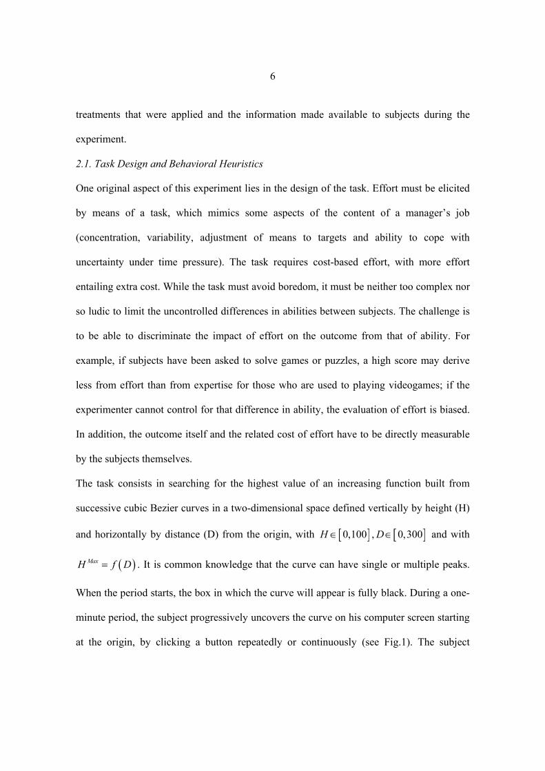
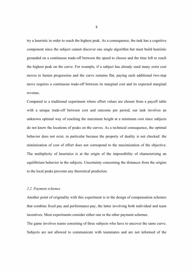
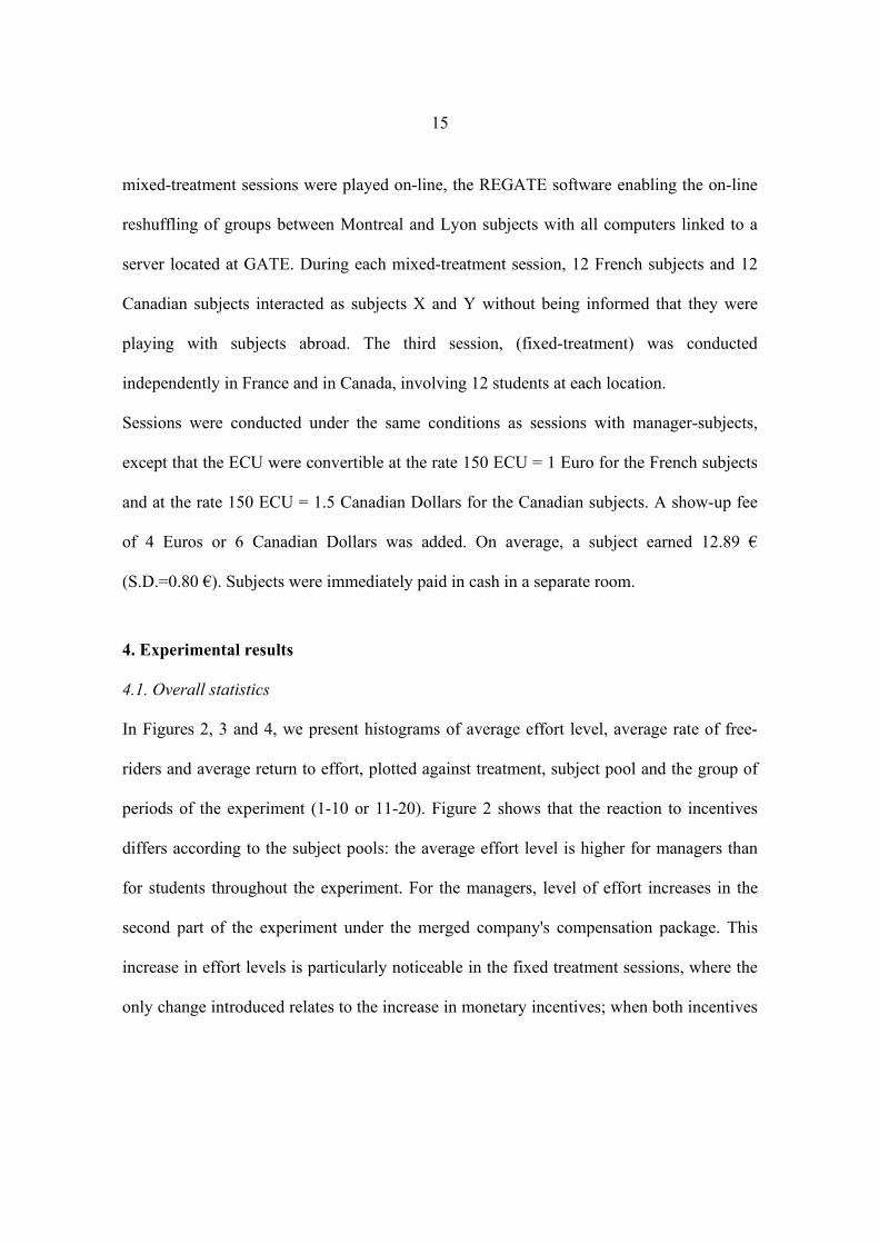
The task consists in searching for the highest value of an increasing function built from

successive cubic Bezier curves in a two-dimensional space defined vertically by height (H)

and horizontally by distance (D) from the origin, with [ ]0,100H ∈ , [ ]0,300D∈ and with

( )MaxH f D= . It is common knowledge that the curve can have single or multiple peaks.

When the period starts, the box in which the curve will appear is fully black. During a one-

minute period, the subject progressively uncovers the curve on his computer screen starting

at the origin, by clicking a button repeatedly or continuously (see Fig.1). The subject

7

discovers the curve by discrete steps on the horizontal axis. Subjects can stop their

progression at any moment. The curve and its surface become visible as the subject

progresses. The outcome achieved by a subject in a period is given by the maximum height

reached on the curve, which depends notably on the number of moves.

[Insert figure 1 about here]

The monetary cost associated with the effort is represented by the choice of the speed of

progression, i.e. the work pace. Parameters are chosen so that it is impossible to reach

maximum height during the one-minute period allowed by using the regular speed only,

with the exception of one of the 13 randomly occurring curves. The subjects do not know

this information. Two buttons are available to the subject: a “1-step button” used to uncover

the curves at one step (regular) speed and is cost free in terms of points; a “2-step button”

that doubles the steps (speed) but which costs 0.4 points. The subject can switch speeds at

will. This design allows a control over the subject’s effort cost and makes possible an

analysis of efficiency.

A subject's outcome depends on the use of two-step moves and on chance since there is

uncertainty about the distances from the origins to the peaks. Therefore, the cognitive

dimension of the task partly relates to the uncertainty about the shape of the curve, partly to

time pressure and partly to the subject’s decision to use the 1-step or 2-step button.

Unlike other real-effort experiment such as van Dijk, Sonnemans and van Winden's (2001),

in which the subject can discover a single peak of a three-dimension convex by using the

gradient method successively following two dimensions, our experiment involves no

algorithm enabling the discovery of a peak at minimum cost while under time constrains. In

our experiment no one benefits from previous learning. Each participant must develop and

8

try a heuristic in order to reach the highest peak. As a consequence, the task has a cognitive

component since the subject cannot discover one single algorithm but must build heuristic

grounded on a continuous trade-off between the speed to choose and the time left to reach

the highest peak on the curve. For example, if a subject has already used many extra cost

moves to hasten progression and the curve remains flat, paying each additional two-step

move requires a continuous trade-off between its marginal cost and its expected marginal

revenue.

Compared to a traditional experiment where effort values are chosen from a payoff table

with a unique trade-off between cost and outcome per period, our task involves an

unknown optimal way of reaching the maximum height at a minimum cost since subjects

do not know the locations of peaks on the curves. As a technical consequence, the optimal

behavior does not exist, in particular because the property of duality is not checked: the

minimization of cost of effort does not correspond to the maximization of the objective.

The multiplicity of heuristics is at the origin of the impossibility of characterizing an

equilibrium behavior in the subjects. Uncertainty concerning the distances from the origins

to the local peaks prevents any theoretical prediction.

2.2. Payment schemes

Another point of originality with this experiment is in the design of compensation schemes

that combine fixed pay and performance-pay, the latter involving both individual and team

incentives. Most experiments consider either one or the other payment schemes.

The game involves teams consisting of three subjects who have to uncover the same curve.

Subjects are not allowed to communicate with teammates and are not informed of the

9

simultaneous progression of their teammates. Each subject has to perform the task on her

own but payoffs depend on both individual and collective outcomes. Individual earnings

from a task in a given period are calculated from the sum of three elements whose amount

and relative proportion depend on the stage of the game and on the treatment. Specifically,

earnings are defined as: i F I Tα α α απ = + + , with { },X Yα = . X and Y correspond to the two

firms before they merge, and for simplicity X and Y subjects keep their respective labels

after the merger in order to track their origin.

• Fα is a fixed-wage earned by subject i when her individual outcome reaches a first

threshold, min1H , defined by the height reached. This threshold can always be

achieved with no cost steps in the time allowed, but this information is not given to

subjects. An employer would consider an effort level below this benchmark as

professional misconduct.

• Iα is an individual bonus earned if i’s outcome reaches a second threshold, min2H

with min min2 1H H> .

• Tα is a team reward obtained when the sum of individual outcomes by the team of

3 subjects reaches a third threshold min3H with min min min

3 2 13 3H H H> > . In contrast

with the two former elements, a subject may earn this reward even though she does

not contribute an effort greater than the effort giving her the fixed wage or the

individual bonus. This situation creates an incentive to free ride by members of the

team.

10

At each repetition of the game, a new curve is randomly drawn, whose shape determines

the extent of uncertainty faced by the subjects. The analysis of performance and costs must

control for the degree of difficulty of the curves. Because of the structure of the

compensation package, the difficulty of a curve depends on the location of the various

thresholds. An index of difficulty is calculated as : d = (D1)2 + (D2 – D1)2 + (D3 – D2) with

D1 being the abscissa at the origin of the first threshold, 2D the abscissa of the second

threshold and 3D the abscissa of the maximum height. The more distant the first threshold

is from the origin and the greater the distance between the first and the second thresholds,

the more difficult it becomes to reach additional rewards.

2.3. Experimental Treatments and Information Conditions

The experiment aims at identifying the separate influences of changes in incentives and in

team composition. To measure the impact of changes in payment schemes after the merger,

an experimental session was designed having two parts of 10 periods each, with a random

order of presentation of 13 payoff curves. In the first part, used as a benchmark, we

reproduce initial payment schemes that were used before the merger; in the second part the

payment scheme in use after the merger is applied. In the first part, we team X and Y

subjects separately, each playing under the payment scheme used in their initial company.

Members of X teams may receive a fixed wage, an individual bonus and a team reward.

Earnings for members of Y teams are derived from a fixed wage and a team reward only

(see Table 1). The proportion of potential total earnings from the fixed wage is higher for Y

subjects than for X subjects, but the same performance is required from all subjects to

11

trigger their fixed payment and team reward. In the second part of the session, the payment

scheme is the one actually used after the merger and is the same for all subjects. It includes

a fixed wage, an individual bonus and a team reward. Compared to the first part, Y subjects

may now receive an individual bonus and X subjects have seen an increase in the value of

their fixed wage. In avoiding a decrease in the absolute level of any pay component of

earnings between the two parts of the session, the maximum earnings all subjects can

obtain is now 120 ECU (Experimental Currency Units) instead of 100. The comparison of

the performance achieved in the two parts of the experimental session enables us to identify

the influence of changes in monetary incentives.

To measure the impact of team composition on performance, a new matching treatment was

introduced in two experimental sessions. This new treatment is referred as the mixed-

treatment, where teams of 3 randomly associated subjects are formed potentially involving

both X and Y subjects. The fixed-treatment used in the first part of all sessions, where X

and Y subjects are teamed exclusively with X and Y subjects, respectively, is maintained in

the second part in one session. The fixed-treatment serves as a benchmark against which

the effect of team composition after the merger can be tested. In all sessions, a strangers

matching protocol is used. It should be noted that in the second part of the session, only

team composition is changed and not the size of the teams (the negative impact on

efficiency of the increasing size of teams in a merger has already been documented by

Camerer and Knez, 1994).

[Insert Table 1 about here]

All subjects, except those playing the fixed treatment, knew of the existence of two

categories of subjects in equal numbers in the room, but they were kept unaware of the

12

meaning of labels X and Y in order to avoid bias. Subjects learned their own identity by

reading the instruction sheet. They were notified that they would keep the same identity

throughout the session. The instruction sheet for the first 10 periods also mentioned that

they were matched with two other subjects belonging to the same category as themselves

and that the composition of groups would within the same category change with each new

period. They were informed that they would never know the identity and the payoff of their

successive teammates.

Subjects knew the description of the task to be performed and the payoff structure

applicable to their category. They were not given information about the payoff structure of

the other category of subjects. They were aware that the same task was to be achieved by

the three members of their group, but they had no current information about the progression

of their teammates on the curve. They were also informed that during play, their screen

would indicate the time currently left, the cumulated cost of their 2-step decisions and the

height of the different thresholds reached. At the end of each period, a historic table would

give each subject feedback on their own outcome, the outcome (cumulative height)

achieved by their group, total cost, amount of compensation obtained, by source, and total

payoff net of costs.

In the second part of the session, periods 11 to 20, subjects were informed about the payoff

structure of the first part for each of the two categories. The new payoff structure common

to all subjects was explained. In one experimental session, on equal number of subjects

from both categories continued to play under the fixed treatment for periods 11 to 20 as in

the first part. In two experimental sessions, subjects drawn in equal numbers from X and Y

13

were informed that during the remaining 10 rounds they could be matched randomly with

members of the other categoryi.

3. Experimental Procedures

The experiment was first conducted with managers of the pharmaceutical company about

two years after the merger and it was later replicated with students of ITECH (Institut

Textile Chimique)- Lyon (France) and HEC (Hautes Études Commerciales) - Montreal

(Canada).

The experiment with manager-subjects was funded by the Human Resources Department of

the new company. This Department recruited executives by emailing a message on

voluntary participation in a scientific experiment to be conducted by researchers from the

National Center for Scientific Research. A sample of 36 volunteer executives with average

annual earnings of 69,000 euros was created, consisting of 18 managers from each

incoming firm. To limit uncontrolled peer group effects, sessions were designed such that

the participants represented a large diversity of departments and came from different

geographical locationsii. This procedure suggests that most people did not know other

session participants.

The experiment was conducted at company headquarters in Paris. All sessions were held on

the same day to limit the dissemination of information. Managers left the premises rapidly

after completion of a session, and thus did not meet participants of subsequent experimental

sessions. In the first two sessions, 12 participants (6X, 6Y) were subjected to the mixed-

treatment protocol (non homogeneous teams for periods 11-20). In a third session, 12

participants played under the fixed-treatment protocol (homogeneous teams for all 20

14

periods). On average, a session lasted 75 minutes including initial instructions and practice

periods. The experiment was computerized using the REGATE program.

Running the experiment with managers required higher payoffs than with traditional

student pools. Transactions were conducted in Experimental Currency Units, with ECU

convertible to Euros at the rate 150 ECU = 4.5 €. A show-up fee of 8 € was added. On

average, a subject earned 51.45 € (S.D.=3.75). Subjects were paid a few days later with

vouchers.

Upon arrival, each manager had to register and was invited to draw a ticket from an

envelope to assign him or her a computer. In fact, company specific envelopes were

presented to subjects according to their originating company, but subjects were unaware of

this allocation rule. At the beginning of the experiment, subjects discovered a set of written

instructions for the first part of the session under their keyboard. As the payment schemes

differed among X and Y participants, the experimenter did not read the instructions aloud

(available upon request)iii. Instructions were phrased in neutral terms (we spoke about a

curve, a group, a payoff, an outcome, and we avoided loaded terms such as effort,

contribution and wage). Participants were allowed to ask questions, which were answered

in private. Three practice rounds were then run before the first part of the experiment

began. At the end of the first part, the game stopped and further instructions for the second

part were distributed, without any questions allowed.

This experiment was replicated with 72 student subjects, in the experimental laboratories of

Groupe d’Analyse et de Théorie Economique (GATE, Lyon, France) and at the laboratory

(LUBC3E) of the Center for Interuniversity Research and ANalysis on Organizations

(CIRANO, Montreal, Canada). Three sessions were organized over two days. The two

15

mixed-treatment sessions were played on-line, the REGATE software enabling the on-line

reshuffling of groups between Montreal and Lyon subjects with all computers linked to a

server located at GATE. During each mixed-treatment session, 12 French subjects and 12

Canadian subjects interacted as subjects X and Y without being informed that they were

playing with subjects abroad. The third session, (fixed-treatment) was conducted

independently in France and in Canada, involving 12 students at each location.

Sessions were conducted under the same conditions as sessions with manager-subjects,

except that the ECU were convertible at the rate 150 ECU = 1 Euro for the French subjects

and at the rate 150 ECU = 1.5 Canadian Dollars for the Canadian subjects. A show-up fee

of 4 Euros or 6 Canadian Dollars was added. On average, a subject earned 12.89 €

(S.D.=0.80 €). Subjects were immediately paid in cash in a separate room.

4. Experimental results

4.1. Overall statistics

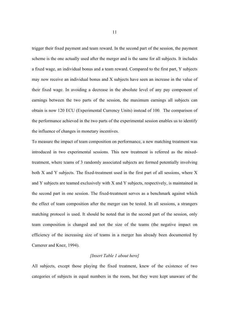
In Figures 2, 3 and 4, we present histograms of average effort level, average rate of free-

riders and average return to effort, plotted against treatment, subject pool and the group of

periods of the experiment (1-10 or 11-20). Figure 2 shows that the reaction to incentives

differs according to the subject pools: the average effort level is higher for managers than

for students throughout the experiment. For the managers, level of effort increases in the

second part of the experiment under the merged company's compensation package. This

increase in effort levels is particularly noticeable in the fixed treatment sessions, where the

only change introduced relates to the increase in monetary incentives; when both incentives

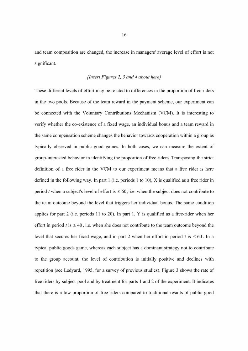
16

and team composition are changed, the increase in managers' average level of effort is not

significant.

[Insert Figures 2, 3 and 4 about here]

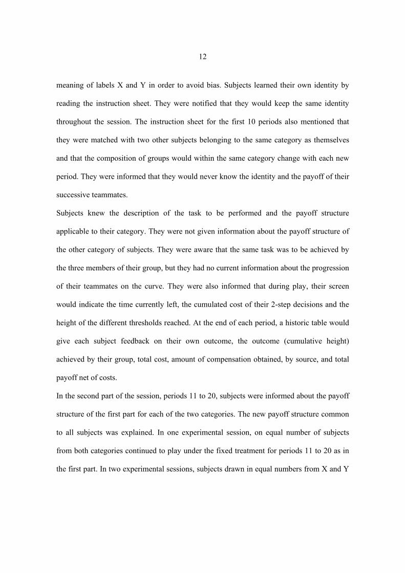
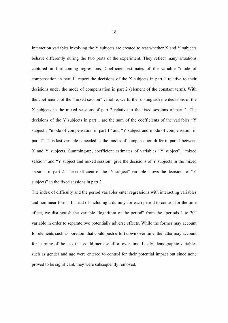
These different levels of effort may be related to differences in the proportion of free riders

in the two pools. Because of the team reward in the payment scheme, our experiment can

be connected with the Voluntary Contributions Mechanism (VCM). It is interesting to

verify whether the co-existence of a fixed wage, an individual bonus and a team reward in

the same compensation scheme changes the behavior towards cooperation within a group as

typically observed in public good games. In both cases, we can measure the extent of

group-interested behavior in identifying the proportion of free riders. Transposing the strict

definition of a free rider in the VCM to our experiment means that a free rider is here

defined in the following way. In part 1 (i.e. periods 1 to 10), X is qualified as a free rider in

period t when a subject's level of effort is 60≤ , i.e. when the subject does not contribute to

the team outcome beyond the level that triggers her individual bonus. The same condition

applies for part 2 (i.e. periods 11 to 20). In part 1, Y is qualified as a free-rider when her

effort in period t is 40≤ , i.e. when she does not contribute to the team outcome beyond the

level that secures her fixed wage, and in part 2 when her effort in period t is 60≤ . In a

typical public goods game, whereas each subject has a dominant strategy not to contribute

to the group account, the level of contribution is initially positive and declines with

repetition (see Ledyard, 1995, for a survey of previous studies). Figure 3 shows the rate of

free riders by subject-pool and by treatment for parts 1 and 2 of the experiment. It indicates

that there is a low proportion of free-riders compared to traditional results of public good

17

games (see Keser and van Winden, 2000), probably because of both the coexistence of

individual and collective payments and the impossibility of calculating the marginal per

capita return of investing in the team outcome. The proportion of free riders is lower among

managers than among students in both part 1 and part 2. This proportion is lower when the

threshold that triggers the greater individual reward is low. It increases in part 2 in both

subject pools, particularly in the mixed sessions, and this cannot be explained by a restart

effect at the 11th period of the game as will be shown later. This is in line with the declining

cooperation over time usually found in public goods experiments and could be compared

with the differences observed between stranger- and partner-matching protocols (see

Croson, 1996, and Keser and van Winden, 2000).

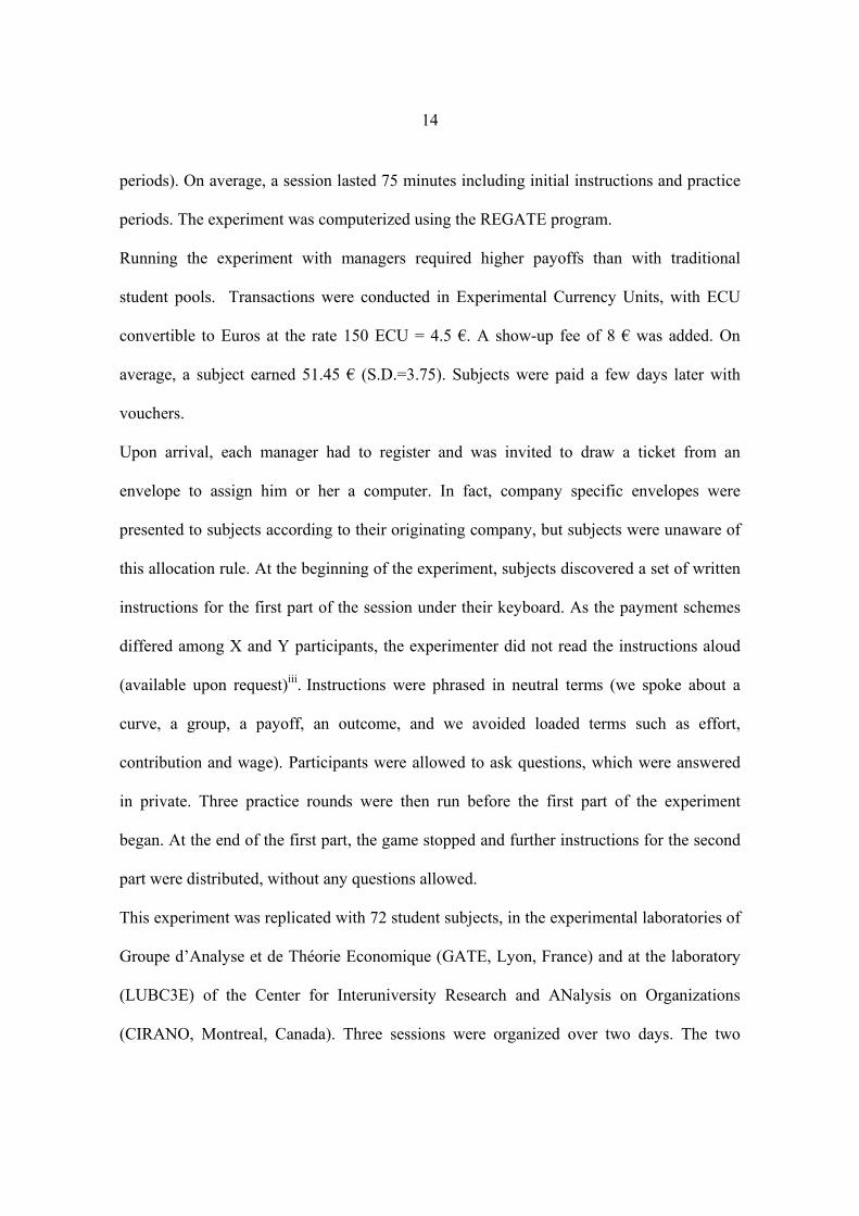
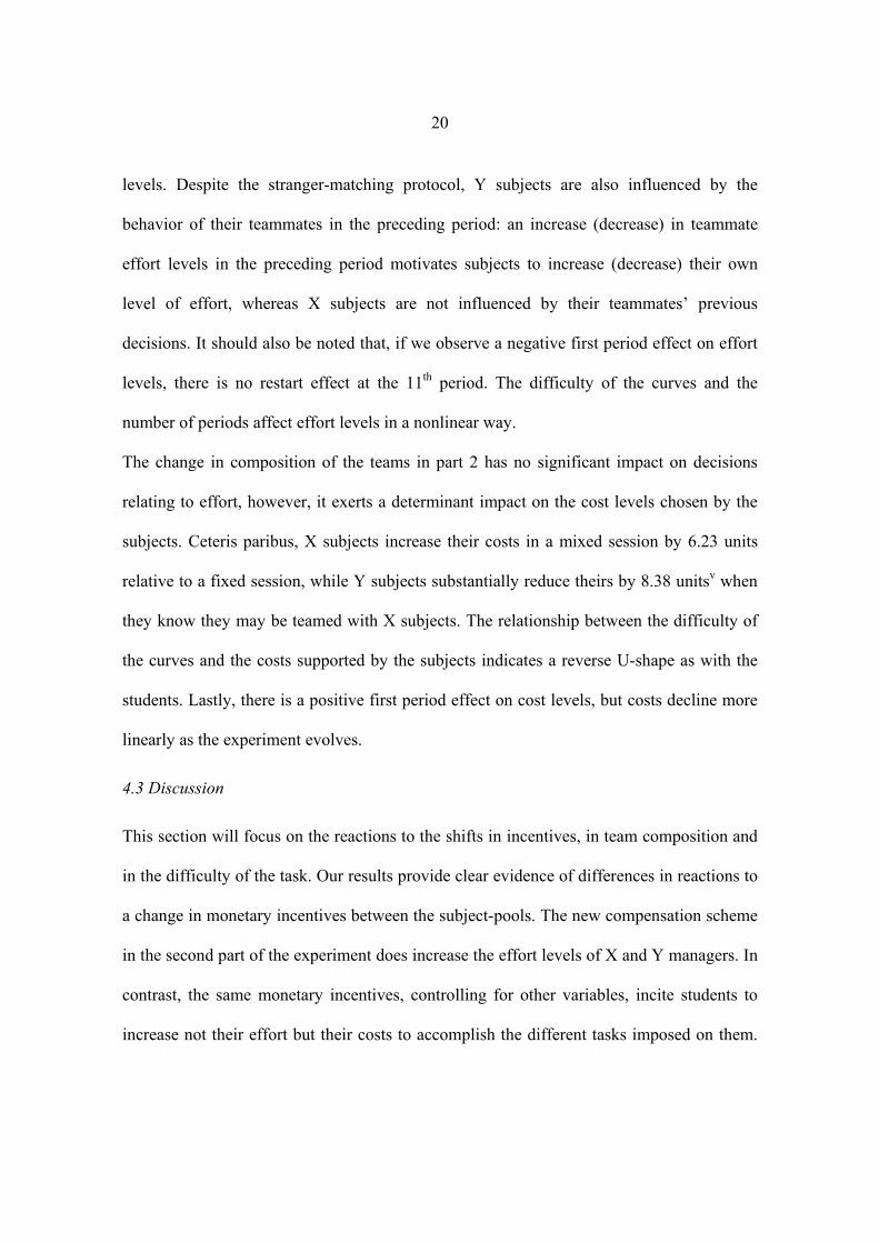
Figure 4 displays the average return to effort, i.e. the average effort level divided by the

average cost level. On average, managers achieve a lower level of efficiency than students.

The former perform a greater effort but at a higher cost. In part 2, the average level of

efficiency rises slightly in both subject pools.

However, overall statistics are uncontrolled for time, difficulty of the curves and individual

effects. Regression analyses controlling for these dimensions are thus required to identify

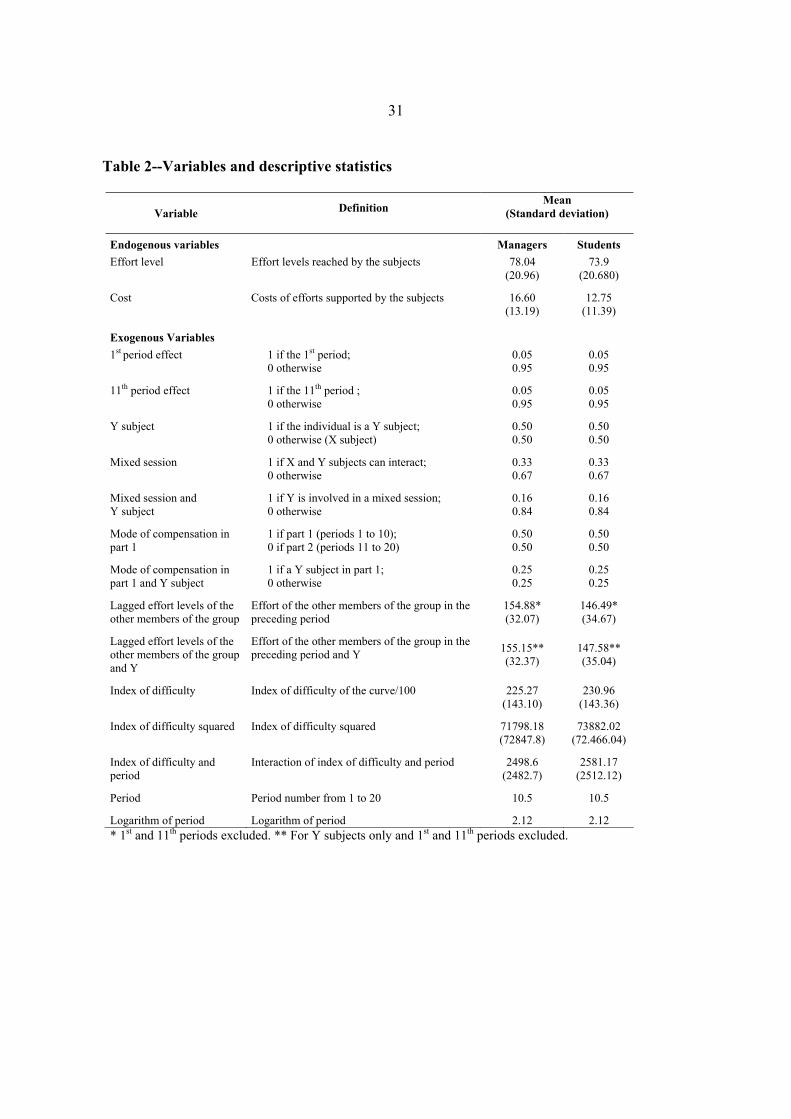
the determinants of two endogenous variables: effort levels and costs. In Table 2, we

present the definition and descriptive statistics of variables used in these regressions.

[Insert Table2 about here]

Exogenous variables are the period, the category of subjects, the mode of compensation, the

composition of groups (either fixed or mixed) and an index of difficulty for each curve. The

“lagged effort level of the other group members” variable assesses whether subjects

modulate their efforts to what their teammates did in the previous period.

18

Interaction variables involving the Y subjects are created to test whether X and Y subjects

behave differently during the two parts of the experiment. They reflect many situations

captured in forthcoming regressions. Coefficient estimates of the variable “mode of

compensation in part 1” report the decisions of the X subjects in part 1 relative to their

decisions under the mode of compensation in part 2 (element of the constant term). With

the coefficients of the “mixed session” variable, we further distinguish the decisions of the

X subjects in the mixed sessions of part 2 relative to the fixed sessions of part 2. The

decisions of the Y subjects in part 1 are the sum of the coefficients of the variables “Y

subject”, “mode of compensation in part 1” and “Y subject and mode of compensation in

part 1”. This last variable is needed as the modes of compensation differ in part 1 between

X and Y subjects. Summing-up, coefficient estimates of variables “Y subject”, “mixed

session” and “Y subject and mixed session” give the decisions of Y subjects in the mixed

sessions in part 2. The coefficient of the “Y subject” variable shows the decisions of “Y

subjects” in the fixed sessions in part 2.

The index of difficulty and the period variables enter regressions with interacting variables

and nonlinear forms. Instead of including a dummy for each period to control for the time

effect, we distinguish the variable “logarithm of the period” from the “periods 1 to 20”

variable in order to separate two potentially adverse effects. While the former may account

for elements such as boredom that could push effort down over time, the latter may account

for learning of the task that could increase effort over time. Lastly, demographic variables

such as gender and age were entered to control for their potential impact but since none

proved to be significant, they were subsequently removed.

19

4.2 Econometric results

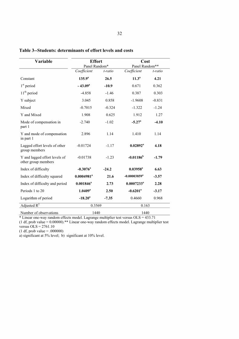
Column 1 of Tables 3 and 3a display the results for the students and managers,

respectively, from a linear one-way random effects model on the subjects’ effort

levelsiv.Column 2 of both tables report the results on the determinants of cost levels decided

by the subjects. The cost incurred corresponds to the number of occasion the 2-steps button

was used to perform the task. The econometric estimates are also obtained with a linear

one-way random effects model.

[Insert Tables 3 and 3a about here]

For the students considered as a benchmark, few variables significantly influence effort

levels, except periods and the difficulty of the task. In contrast, the cost levels are

influenced by more elements. A change in monetary incentives in the second part of the

experiment (a higher maximum pay and a new structure of compensation) makes students

react by increasing their cost levels but not their effort. An increase in the effort levels of

their teammates during the preceding period incites them to increase their costs, particularly

for the X subjects. Lastly, costs decline over time and the relationship between the

difficulty of the curves and the costs indicates a reverse U-shape.

In contrast, we observe for managers a significant and substantial increase in effort levels

by both X and Y subjects in part 2 relative to part 1. The change in incentives after the

merger increases effort levels by almost 12 points. The change in the composition of teams

exerts no significant influence on effort. Note however the negative but statistically

insignificant coefficient of the interaction variable “Y subject and Mixed”: Y subjects,

knowing that they may be interacting with X subjects, have a tendency to lower their effort

20

levels. Despite the stranger-matching protocol, Y subjects are also influenced by the

behavior of their teammates in the preceding period: an increase (decrease) in teammate

effort levels in the preceding period motivates subjects to increase (decrease) their own

level of effort, whereas X subjects are not influenced by their teammates’ previous

decisions. It should also be noted that, if we observe a negative first period effect on effort

levels, there is no restart effect at the 11th period. The difficulty of the curves and the

number of periods affect effort levels in a nonlinear way.

The change in composition of the teams in part 2 has no significant impact on decisions

relating to effort, however, it exerts a determinant impact on the cost levels chosen by the

subjects. Ceteris paribus, X subjects increase their costs in a mixed session by 6.23 units

relative to a fixed session, while Y subjects substantially reduce theirs by 8.38 unitsv when

they know they may be teamed with X subjects. The relationship between the difficulty of

the curves and the costs supported by the subjects indicates a reverse U-shape as with the

students. Lastly, there is a positive first period effect on cost levels, but costs decline more

linearly as the experiment evolves.

4.3 Discussion

This section will focus on the reactions to the shifts in incentives, in team composition and

in the difficulty of the task. Our results provide clear evidence of differences in reactions to

a change in monetary incentives between the subject-pools. The new compensation scheme

in the second part of the experiment does increase the effort levels of X and Y managers. In

contrast, the same monetary incentives, controlling for other variables, incite students to

increase not their effort but their costs to accomplish the different tasks imposed on them.

21

Among managers, Y participants substantially decrease their costs in part 2. Another

difference is the reaction to lagged effort levels of the other group members. Y managers

increase (decrease) their effort if the effort levels of their previous teammates increase

(decrease). Student participants do not adjust their effort levels to that of others but modify

their cost levels to the previous effort levels of their group members.

These results show that the change in incentives influences both subject-pools, with

managers appearing to be objective driven while students are cost driven. This is not that

surprising as managers in their professional life are evaluated, remunerated and promoted

by meeting their objectives whatever the cost they must incur to do so (long working hours

for example). For most students, a large part of the return of their academic effort is from

lowering their cost (time devoted to studying a specific matter) in order to obtain good

grades. Note that we were able to observe this kind of results because we used a real cost

task with time constraints. If the student-subjects appear to be more money maximizing

than managers in the laboratory, this cannot be attributed to the differences in the

opportunity costs to participate, since this was taken into account in the conversion rates.

The changing composition of teams also influences the behavior of subjects. Within the

same category (X or Y), most subjects are influenced by the behavior of their preceding

teammates although teams are reshuffled each period. This might suggest that the subjects

refer to their category as a whole. However, the linear one-way effects models used to

explain effort and cost levels recognized that subjects are heterogeneous; our results

suggest that subject-pools and categories are also heterogeneous. Both X and Y student-

subjects are influenced by the effort of the subjects they were previously teamed with but

they are not influenced by the merging between categories in the second part of the

22

experiment; thus, they do not refer to a specific category but to a whole set of subjects in

the laboratory. By contrast, after the merger, the decisions of the category of managers who

are more sensitive to the efforts of previous teammates (the Y managers) change behavior

knowing that they may be interacting with subjects from the other category; they become

less cooperative and they substantially reduce their costs and to a lesser degree their effort.

On the contrary, X managers who are not influenced by the behavior of previous teammates

react positively to the merging of the categories in the same teams. Groups of reference are

not the same across subject-pools.

In traditional experimental economics literature, reaction to others’ decision is usually

characterized by a reciprocity concept (see Fehr and Falk, 2002). Since our experiment is

run with randomly re-matched subjects at each period, this can also be explained by

learning and conditional cooperation: subjects learn the behavior of other subjects in the

same category or in the same room and constantly update their evaluation of the behavior

of their potential teammates. But more puzzling is the reaction to the mixing of categories

after the merger. Three explanations could be evoked. A first explanation might be that the

merger changes the preferences of the subjects by introducing new incentives. This

explanation cannot help since we measure the impact of a shift in team composition other

things equal, i.e. we control for changes in incentives. The psychological concept of “in-

group/out-group” might affect the cooperative behavior of participants (see Tajfel, Flament,

Billig and Bundy, 1971). This explanation cannot directly help here since students and

managers do not react in the same way. If managers were able to transfer their experience

of the merger into the laboratory whereas the students were not able to do so (Canadian

students were not aware of interacting with French subjects and vice versa), this

23

psychological effect might play a role for the managers. But it does not explain why X and

Y managers did not react similarly. The last and most convincing explanation refers to a

sorting or a selection effect. The incoming companies that merged might differ in recruiting

different profiles of managers, then developing different cultures, because of their various

incentive schemes. The pre-existence of an individual bonus may contribute to focusing on

one’s own performance instead on the other’s effort. This sorting effect of incentives has

been documented by Lazear (2000) in the context of a natural experiment.

The reaction to the difficulty of the task is similar for managers and students. The observed

U-shape curve suggests that across all compensation schemes, more difficult tasks may

actually elicit, to some extent, more effort by all types of participants. This job challenge

effect is present even in the later stages of the experiment (see the “index of difficulty and

period” crossed variable). This result is consistent with the psychological literature showing

that challenging goals lead to higher performance than easy goals (Locke, Saari, Shaw and

Latham, 1981). The job challenge may even be at the initiative of the subject herself (for

example if she uses targets like reaching the second peak). These relationships also suggest

that the production of effort as a function of the degree of difficulty changes over time:

while the logarithm of period (that could be interpreted as boredom or tiredness) exerts a

negative effect on the production of effort, the agent reacts more and more to job challenge

over time.

The relationship between the difficulty of the curves and the costs supported by all

participants indicates a reverse U-shape. If the task is too difficult, subjects increase their

efforts but without resorting to costly 2-step moves. This result reinforces our preceding

24

analysis: an increased difficulty does not discourage effort under the condition that subjects

can save on their costs. Lastly, there is a positive first period effect on the cost levels

(significant for the managers), but costs decline more linearly as the experiment evolves.

This is possibly due to a learning effect on the task, on the other’s behavior, and on the best

moment to use the costly 2-step moves. Students appear to learn more than managers as

they play the game since they not only decrease their costs but also increase their efforts

(see variable “Period 1 to 20”). Overall, along with their cost driven strategy, they realize a

better average return to effort than managers, as shown earlier.

5. Summary and conclusions

Executive behavior with respect to performance, motivation and cooperation is a major

element in the success or failure of a merger between companies. Traditionally, economists

have suggested looking for an adapted compensation policy to facilitate cooperation and

renewed effort from groups of individuals coming from different corporate cultures. The

aim of this paper is to check whether a harmonization of compensation packages is

sufficient to motivate all managers to cooperate to the same extent. A laboratory

experiment has been run involving managers of two large pharmaceutical companies that

recently went through a merger. The experimental design has introduced various

compensation schemes, including an incentive scheme combining individual and team

incentives that were implemented in the context of a real effort. As in most mergers, these

manager-subjects have experienced the redesigning of both compensation schemes and

team composition in their newly merged company. The experimental protocol reproduced

the pre- and post-merger situation both in terms of compensation and in terms of team

25

composition. To complement this experiment with managers, a replication with a subject

pool consisting of French and Canadian students was conducted that can serve as a

benchmark.

The results show that financial incentives do work in improving effort among managers, in

accordance with standard results (Prendergast, 1999). However, the unified incentives are

not entirely sufficient to create cooperation among heterogeneous groups, as already

experimentally observed (Meidinger, Rulliere and Villeval, 2003). The past matters. In

contrast with Nalbantian and Schotter (1997), it matters more in terms of shifting team

composition than in terms of incentives, since the change from the two pre-merger

incentive schemes to the unified one increases effort in the same proportion for both

categories of managers. Individuals coming from different corporate cultures, likely with

different fairness norms and social comparison behavior, tend to react differently in the

mixed treatment part of our experiment. This may result notably from a sorting effect,

attributable to various manager selection policies in the originating firms: companies with

different incentive policies will probably attract different types of managers. This suggests

that shifting team composition may limit, at least in the short run, the efficiency of a new

unified compensation policy, if not taken into account. Merging cultures requires more time

than merging incentives and deserves special attention. This is probably more accurate in

the case of mergers than in the case of other kinds of restructuring policies.

Results from the student-subject pool differ in strategy more than in substance, allowing

confirmation of the external validity of laboratory experiments. In contrast to the managers,

students react to an increase in monetary incentives by accepting more costs to complete a

given task rather than increasing their effort levels. They are cost driven whereas managers

26

appear to be objective-driven. Being objective-driven means that the managers are also

more cooperative and free ride less than the student-subjects. Our results corroborate the

interpretation of Cooper et al. (1999) in that when they are able to recognize the similarity

between the laboratory context and their field experience, manager-subjects may choose

different strategic options than inexperienced subjects. Moreover, it may indicate that if

students are more inclined to minimize costs than experts in the laboratory, when one

observes the existence of other-regarding preferences in traditional experiments involving

student-subjects, one may deduce that this deviation from the equilibrium is likely even

more developed in real settings.

Lastly, our experiment shows that introducing a complex task is not necessarily detrimental

to more effort and cooperation. The concept of job challenge is perhaps more important to

soliciting greater effort among employees than is usually suggested in current literature.

27

Figure 1. An example of a typical curve

Figure 2. Average effort by subject pool and by treatment

70

72

74

76

78

80

82X Students 1-10

Y Students 1-10

Mixed Students 11-20

Fixed Students 11-20

X Managers 1-10

Y Managers 1-10

Mixed Managers 11-20

Fixed Managers 11-20

28

Figure 3. Average proportion of free riders by subject pool and by treatment

0

5

10

15

20

25

30

35 X Students 1-10Y Students 1-10Mixed Students 11-20 Fixed Students 11-20

X Managers 1-10Y Managers 1-10Mixed Managers 11-20 Fixed Managers 11-20

4

4,5

5

5,5

6

6,5X Students 1-10

Y Students 1-10

Mixed Students 11-20

Fixed Students 11-20

X Managers 1-10

Y Managers 1-10

Mixed Managers 11-20

Fixed Managers 11-20

29

Figure 4. Average return to effort by subject pool and by treatment

Note: The average indices of difficulty of the curves are the following: In the student-sessions, periods 1 to 10: 22 949; periods 11-20 in the mixed treatment: 24 047; periods 11-20 in the fixed sessions: 21 635. In the manager-sessions, periods 1 to 10: 22 949; periods 11-20 in the mixed treatment: 22 339; periods 11-20 in the fixed sessions: 21 635.

30

Table 1-- Payment schemes in ECU

Part 1 – All treatments Part 2 – Fixed treatment Part 2 – Mixed treatment Group Composition

Teams of X subjects

Teams of Y subjects

Teams of X subjects

Teams of Y subjects

Teams of X and Y subjects

Height reached 40iH <

40 60iH≤ <

60 100iH≤ ≤

3

1240iH ≥∑

0 40 60

100

0 60 60

100

0 60 80

120

0 60 80

120

0 60 80

120

Note: For the teams of X subjects the table should be read as follows. In the first part of the experiment, if a X subject realizes an outcome lower than the first threshold of 40, he receives no payoff. If he reaches a height between the first (40) and the second threshold (60), he receives only a fixed wage of 40 ( XF ). If the subject reaches the second threshold, he receives a payoff of 60, consisting of the sum of the fixed wage and the individual bonus ( X XF I+ ). If the subject’s team reaches a cumulated height of 240, the subject receives a payoff of 100, corresponding to the sum of the fixed wage, the individual bonus and the team reward ( X X XF I T+ + ). Part 2 and the teams of Y subjects should be interpreted in a similar manner.

31

Table 2--Variables and descriptive statistics

Variable Definition Mean

(Standard deviation)

Endogenous variables Managers Students Effort level Effort levels reached by the subjects 78.04

(20.96) 73.9

(20.680)

Cost

Costs of efforts supported by the subjects 16.60 (13.19)

12.75 (11.39)

Exogenous Variables 1st period effect

1 if the 1st period; 0 otherwise

0.05 0.95

0.05 0.95

11th period effect

1 if the 11th period ; 0 otherwise

0.05 0.95

0.05 0.95

Y subject 1 if the individual is a Y subject; 0 otherwise (X subject)

0.50 0.50

0.50 0.50

Mixed session

1 if X and Y subjects can interact; 0 otherwise

0.33 0.67

0.33 0.67

Mixed session and Y subject

1 if Y is involved in a mixed session; 0 otherwise

0.16 0.84

0.16 0.84

Mode of compensation in part 1

1 if part 1 (periods 1 to 10); 0 if part 2 (periods 11 to 20)

0.50 0.50

0.50 0.50

Mode of compensation in part 1 and Y subject

1 if a Y subject in part 1; 0 otherwise

0.25 0.25

0.25 0.25

Lagged effort levels of the other members of the group

Effort of the other members of the group in the preceding period

154.88* (32.07)

146.49* (34.67)

Lagged effort levels of the other members of the group and Y

Effort of the other members of the group in the preceding period and Y 155.15**

(32.37) 147.58** (35.04)

Index of difficulty Index of difficulty of the curve/100 225.27 (143.10)

230.96 (143.36)

Index of difficulty squared Index of difficulty squared 71798.18 (72847.8)

73882.02 (72.466.04)

Index of difficulty and period

Interaction of index of difficulty and period 2498.6 (2482.7)

2581.17 (2512.12)

Period Period number from 1 to 20 10.5 10.5

Logarithm of period Logarithm of period 2.12 2.12 * 1st and 11th periods excluded. ** For Y subjects only and 1st and 11th periods excluded.

32

Table 3--Students: determinants of effort levels and costs

Variable Effort Panel Random*

Cost Panel Random**

Coefficient t-ratio Coefficient t-ratio

Constant 135.9a 26.5 11.3a 4.21

1st period - 43.09a -10.9 0.671 0.362

11th period -4.858 -1.46 0.387 0.303

Y subject 3.045 0.858 -1.9608 -0.831

Mixed -0.7015 -0.324 -1.322 -1.24

Y and Mixed 1.908 0.625 1.912 1.27

Mode of compensation in part 1

-2.740 -1.02 -5.27a -4.10

Y and mode of compensation in part 1

2.896 1.14 1.410 1.14

Lagged effort levels of other group members

-0.01724 -1.17 0.02892a 4.18

Y and lagged effort levels of other group members

-0.01738 -1.23 -0.01186b -1.79

Index of difficulty -0.3076a -24.2 0.03958a 6.63

Index of difficulty squared 0.0004981a 21.6 -0.00003859a -3.57

Index of difficulty and period 0.001846a 2.73 0.0007233a 2.28

Periods 1 to 20 1.0409a 2.50 -0.6201a -3.17

Logarithm of period -18.20a -7.35 0.4660 0.968

Adjusted R2 0.3569 0.163

Number of observations 1440 1440 * Linear one-way random effects model. Lagrange multiplier test versus OLS = 433.71 (1 df, prob value = 0.00000).** Linear one-way random effects model. Lagrange multiplier test versus OLS = 2761.10 (1 df, prob value = .000000) a) significant at 5% level; b) significant at 10% level.

33

Table 3a--Managers: determinants of effort levels and costs

Variable Effort Panel Random*

Cost Panel Random**

Coefficient t-ratio Coefficient t-ratio

Constant 125.32a 13.3 6.197 1.13

1st period - 11.80 -1.59 10.25a 2.42

11th period -1.539 -0.289 0.967 0.318

Y subject -3.030 -0.526 8.06a 2.16

Mixed 1.500 0.414 6.23a 2.83

Y and Mixed -7.194 -1.41 -14.61a -4.69

Mode of compensation in part 1

-11.791a -2.47 -1.805 -0.653

Y and mode of compensation in part 1

-4.559 -1.04 -10.09a -3.88

Lagged effort levels of other group members

0.03469 1.251 0.02427 1.53

Y and lagged effort levels of other group members

0.05420a 2.33 0.0195 1.37

Index of difficulty -0.2132a -9.41 0.05503a 4.27

Index of difficulty squared 0.0003381a 8.37 -0.00007559a -3.29

Index of difficulty and period 0.003394a 2.82 0.001122b 1.64

Periods 1 to 20 -1.354b -1.83 -1.037a -2.47

Logarithm of period -7.768b -1.76 2.799 1.11

Adjusted R2 0.1562 0.1792

Number of observations 720 720 * Linear one-way random effects model. Lagrange multiplier test versus OLS = 12.06 (1 df, prob value = .000515). ** Linear one-way random effects model. Lagrange multiplier test versus OLS = 114.41 (1 df, prob value = .000000). a) significant at 5% level; b) significant at 10% level.

34

Notes

i It would have been interesting to test whether belonging to the majority category or the

minority category of a team would influence individual behavior within teams. However,

this would have required collecting a far greater number of observations. For this reason we

did not inform subjects about the detailed composition of their teams.

ii Overall, participants came from 4 different sites and 22 departments.

iii Reading instructions aloud guarantees that rules are common knowledge. However the

section of instructions related to different payment schemes of the X and Y subjects must

remain unknown until the end of the first part of the session. Reading aloud only other

sections of the instructions would have focused undue attention on the question of

compensation.

iv Let itE measure individual i’s level of effort in period t, explained by a vector of

observable variables zit, the corresponding parameter vector δ, a random individual

component iη and a random variable itε :

TtnizE iititit ,,1,,,1, KK ==++= ηεδ with the usual assumptions,

( ) ( ) .0,,0~,1,0~ 2 =εησσηε NN itit

v This result derives from the following calculation: [8.06 – (8.06 + 6.23 – 14.61)]. The first

term corresponds to the coefficient of the variable for Y participants in part 2 when groups

are fixed. The second term represents the value of the coefficients for Y participants in part

2 when groups are mixed.

35

References

Bull, C., Schotter, A., Weigelt, K., 1987.Tournaments and Piece-Rates: An experimental

Study. Journal of Political Economy 95, 1-33.

Camerer, C.F., Knez, M., 1994. Creating “expectational assets” in the laboratory: “weakest-

link” coordination games. Strategic Management Journal 15, 101-119.

Carpenter, J., Burks, S., Verhoogen, E., 2003. Comparing Students to Workers: The Effects

of Social Framing on Behavior in Distribution Games Mimeo, Middlebury College.

Cooper, D.J., Kagel, J.H., Lo, W., Gu, Q.L., 1999. Gaming against managers in Incentive

Systems: Experimental Results with Chinese Students and Chinese Managers. American

Economic Review 89(4), 781-804.

Croson, R.T.A., 1996. Partners and Strangers Revisited. Economics Letters 53(1), 25-32.

Dickinson, D.L., 1999. An Experimental Examination of Labor Supply and Work

Intensities. Journal of Labor Economics 17 (4), 608-638.

Dyer, D., Kagel, J.H., Levin, D., 1989. A Comparison of Naive and Experienced Bidders in

Common Value Offer Auctions: A Laboratory Analysis. The Economic Journal 99, 108-

115.

Erev, I., Bornstein, G., Galili, R., 1993. Constructive Intergroup Competition as Solution to

the Free Rider Problem: A Field Experiment. Journal of Experimental Social Psychology

29, 463-478.

Falk, A., Ichino, A., 2003. Clean Evidence on Peer Pressure. IZA Discussion Paper 732,

Bonn.

Fehr, E., Gächter, S., Kirchsteiger, G., 1997. Reciprocity as a Contract Enforcement

Device: Experimental Evidence. Econometrica 65, 833-860.

36

Fehr, E., Falk, A., 2002. Psychological Foundations of Incentives. European Economic

Review 46, 687-724.

Fehr, E., List, J.A., 2002. The Hidden Costs and Returns of Incentives – Trust and

Trustworthiness among CEOs. Institute for Empirical Research in economics, University of

Zurich, Working Paper n°14.

Gneezy, U., Niederle, M., Rustichini, A., 2003. Performance in Competitive Environments:

Gender Differences. Quarterly Journal of Economics, August, 1049-1074.

Güth, Königstein, Kovacs and Zala-Meso, 2001.

Hannan, R.L., Kagel, J.H., Moser, D.V., 2002. Partial Gift Exchange in an Experimental

Labor Market: Impact of Subject Population Differences, Productivity Differences, and

Effort Requests on Behavior. Journal of Labor Economics 20(4), 923-951.

Harrison, G.W., List, J.A., 2003. What Constitutes a Field Experiment in Economics?

University of Central Florida and University of Maryland, mimeo.

Hermalin, B.E., Wallace, N.E., 2001. Firm performance and Executive Compensation in

the Savings and Loan Industry. Journal of Financial Economics 61, 139-170.

Keser, C., van Winden, F., 2000. Conditional Cooperation in Voluntary Contributions to

Public Goods. Scandinavian Journal of Economics 102(1), 23-39.

Kreps, D., 1990. Corporate Culture and Economic Theory. In J. Alt and K. Schepsle (Eds.),

Perspective on Positive Political Economy, Cambridge, Cambridge University Press, 90-

143.

Lazear, E.P., 2000. Performance Pay and Productivity. American Economic Review 90 (5),

1346-1361.

Ledyard, J.O., 1995. Public Goods: A Survey of Experimental Research, in J.H. Kagel and

37

A.E. Roth (Eds.), Handbook of Experimental Economics, Princeton, Princeton University

Press, 111-194.

Locke, E.A., Saari, L.M., Shaw, K.N., Latham, G.P., 1981. Goal Setting and Task

Performance: 1969-1980. Psychological Bulletin 90 (1), 125-152.

Meidinger, C., Rulliere, J.L., Villeval, M.C., 2003. Does Team-Based Compensation Give

Rise to Problems when Agents Vary in Their Ability? Experimental Economics 6, 253-272.

Nalbantian, H.R., Schotter, A., 1997. Productivity under Group Incentives: An

Experimental Study. American Economic Review 87, 314-341.

Prendergast, C., 1999. The Provision of Incentives in Firms. Journal of Economic

Literature XXXVII (1), 7-63.

Schotter, A., 1998. Worker trust, system vulnerability, and the performance of work

groups. In A. Ben-Ner and L. Putterman (Eds.), Economics, Values and Organization.

Cambridge, Cambridge University Press, 364-407.

Shearer, B., 2001. Piece-Rates, Fixed Wages and Incentives: Evidence from a Field

Experiment. Université Laval, Québec, Working Paper.

Sillamaa, M.A., 1999. How Work Effort Responds to Wage Taxation: An Experimental

Test of a Zero Top Marginal Tax Rate. Journal of Public Economics 73, 125-134.

Tajfel, H., Flament, C., Billig, M.G., Bundy, R.P., 1971. Social Categorization and

Intergroup Behavior. European Journal of Social Psychology 1, 147-175.

Van Dijk, F., Sonnemans, J., van Winden, F., 2001. Incentives Systems in a Real Effort

Experiment. European Economic Review 45, 187-214.

Weber, R.A., Camerer, C.F., 2003. An Experimental Approach to the Study Culture.

Management Science. In Press.

38

39

Instructions for Redesigning Teams and Incentives: A Real Effort Experiment

with Managers of a Merged Company

Instructions for X participants in the mixed-treatment – Part 1

You are going to participate in an experiment about incentives in work organization, which is part of a scientific program supported by your company and by the CNRS (French National Center for Scientific Research).

During this experimental session, you can earn money. The amount of your earnings depends not only on your decisions, but also on the decisions of the other participants with whom you will interact.

This session consists in 2 parts of 10 periods each. The session should last about one hour. During this session, transactions are conducted in ECU (Experimental Currency Units). Your final earnings are equal to the sum of the ECU you will earn in each of the 20 periods. At the end of the session, the total amount of ECU you have earned will be converted to Euros at the following rate:

10 ECU = 0.30 €

In addition, you will receive a show-up fee of 7,60 €. Your entire earnings from the experiment will be paid in vouchers that will be given to you in a few days.

At the beginning of the session, the group of participants is subdivided into two categories: X and Y participants. You are an X participant. X or Y, you keep the same role throughout this session. Periods 1-10

What does occur in each period? In each period, which lasts 1 minute, each participant has to perform a task on his or her computer.

The task consists in uncovering a curve where a line has been plotted beforehand.

This curve is increasing and/or flat but it never decreases. It can have single or multiple peaks, with a maximum of 3 peaks that are ranked from the lowest to the highest. The highest altitude that can be reached by this curve is 100.

You uncover the line of this curve as you move along. Starting from point 0, you are make progress at the same time in terms of distance (you go along the horizontal axis) and in terms of altitude (you go up on the vertical axis). Time starts running as soon as you click the “OK” button. You can move by clicking one of the two buttons offered on your computer screen. These two buttons correspond to two available speeds.

A first button enables you to take steps of 1. Steps of 1 do not cost money. A second button enables you to take steps of 2. These steps are twice as rapid as steps of 1,

but each step of 2 costs 0.4 ECU. You may switch speed whenever you want and as many times as you like. As long as you do not want to change your speed, you can hold the mouse down and the progression along the curve automatically proceeds at the chosen speed. You can stop your progression whenever you like, even before the one-minute time is over.

When a new period starts, you have to uncover a different curve.

40

With whom do you interact? In each period, you are a member of a team made-up of three people who belong to the same category. In other words, an X participant is necessarily matched with two X participants and a Y participant is necessarily matched with two Y participants. The other two members of your group have to uncover the same curve as you do on their computer screen but none of you knows the current position or the progression of the two other members of the group. For each new period, the composition of the group is changed. However, if you are an X participant, you are still teamed up with X participants, and if you are a Y participant, you are still teamed up with Y participants. How are your earnings determined? Your earnings for each period depend on the following elements:

your own result, which corresponds to the altitude reached on the curve when you stop your progression or when the time is over; this means that only altitude matters; distance does not matter;

the result of your group, i.e. the sum of the altitudes reached by the three members of your group;

the number of steps of 2 that you made, since these steps cost money. You are an X participant. The earnings of an X participant are determined as follows:

Conditions Earnings of X participant If your own outcome reaches: • an altitude lower than 40 • an altitude between 40 and 59 • an altitude between 60 and 100

your gross payoff is: • 0 ECU • 40 ECU • a first complement of 20 ECU is added, i.e.

your gross total payoff is 60 ECU If the sum of the altitudes

achieved by the 3 members of your group reaches at least 240

you receive a second complement of 40 ECU. Your total gross payoff is then 100 ECU.

Beware: the total cost linked to the steps of 2 that you have used will be subtracted from this gross payoff. What information do you receive for each period? During each period, you are informed of the following elements via your computer screen:

the moment your result has reached the altitudes of 40, 60 and 100

the time remaining

the cumulated cost of steps of 2

In addition, as you are moving along the curve: the surface of the curve is colored in blue until the altitude that triggers the first payoff

is reached (from altitude 0 to altitude 39 inclusively); the surface of the curve is colored in yellow as soon as the altitude that triggers the first

payoff is reached and until the altitude that triggers the first complement is reached (from altitude 40 to altitude 59);

beyond that, the surface of the curve is colored in green (from altitude 60 to 100). In other words, as long as the surface of the curve is blue, your gross payoff is null (you may even loose money if you have used steps of 2). When the curve becomes yellow, your gross payoff amounts to 40. When the curve becomes green, your gross payoff is 60 ECU and,

41

depending on the cumulated altitude reached by you and the two other members of your group, you will be informed at the end of the period of whether you have reached the second complement that yields a total gross payoff of 100 ECU or not.

At the end of each period, a summary table indicates for each past period:

your final altitude

the cumulated altitude of your group

the total cost of steps of 2 that you used

whether you have reached the first payoff of 40 ECU and the first complement of 20 ECU

whether the cumulated result of your group enables you to get the second complement of 40 ECU

your total net earnings.

*** If you have any questions regarding these instructions, please raise your hand. Someone will answer your questions privately. Throughout the entire session, talking is not allowed. As soon as everybody is ready, we will begin with 3 practice periods, in order for you to familiarize yourself with the task at hand. The results of these practice periods will not be taken into account in your earnings.

Thank you for your participation.

***

Instructions for Y participants in the mixed-treatment – Part 1

You are going to participate in an experiment about incentives in work organization that is part of a scientific program supported by your company and by the CNRS.

During this experimental session, you can earn money. The amount of your earnings depends not only on your decisions, but also on the decisions of the other participants with whom you will interact.

This session consists in 2 parts of 10 periods each. The session should last about one hour. During this session, transactions are conducted in ECU (Experimental Currency Units). Your final earnings are equal to the sum of the ECU you will earn in each of the 20 periods. At the end of the session, the total amount of ECU you have earned will be converted to Euros at the following rate:

10 ECU = 0.30 €

In addition, you will receive a show-up fee of 7,60 €. Your entire earnings from the experiment will be paid in vouchers that will be given to you in a few days.

At the beginning of the session, the group of participants is subdivided into two categories: X and Y participants. You are a Y participant. X or Y, you keep the same role throughout this session.

42

Periods 1-10

What does occur in each period? In each period, which lasts 1 minute, each participant has to perform a task on his or her computer.

The task consists in uncovering a curve, where a line has been plotted beforehand. This curve is increasing and/or flat but it never decreases. It can have single or multiple peaks, with a maximum of 3, which are ranked from the lowest to the highest. The highest altitude that can be reached by this curve is 100.

You uncover the line of this curve as you move along. Starting from point 0, you make progress at the same time in terms of distance (you go along the horizontal axis) and in terms of altitude (you go up on the vertical axis). Time starts running as soon as you click the “OK” button. You can move by clicking one of the two buttons offered on your computer screen. These two buttons correspond to two available speeds.

A first button enables you to take steps of 1. Steps of 1 do not cost money. A second button enables you to take steps of 2. These steps are twice as rapid as steps of 1,

but each step of 2 costs 0.4 ECU. You may switch speed whenever you want and as many times as you like. As long as you do not want to change your speed, you can hold the mouse down and the progression along the curve automatically proceeds at the chosen speed. You can stop your progression whenever you like, even before the one-minute time is over. When a new period starts, you have to uncover a different curve. With whom do you interact? In each period, you are member of a team made-up of three people who belong to the same category. In other words, an X participant is necessarily matched with two X participants and a Y participant is necessarily matched with two Y participants.

The other two members of your group have to uncover the same curve as you do on their computer screen but none of you knows the current position or the progression of the two other members of the group. For each new period, the composition of the group is changed. However, if you are an X participant, you are still teamed up with X participants, and if you are a Y participant, you are still teamed up with Y participants. How are your earnings determined? Your earnings for each period depend on the following elements:

your own result, which corresponds to the altitude reached on the curve when you stop your progression or when the time is over; this means that only altitude matters; distance does not matter;

the result of your group, i.e. the sum of the altitudes reached by each of the three members of your group;

the number of steps of 2 that you made, since these steps cost money. You are a Y participant. The earnings of a Y participant are determined as follows:

Conditions Earnings of Y participant

43

If your own result reaches: • an altitude lower than 40 • an altitude between 40 and 100

your gross payoff is: • 0 ECU • 60 ECU

If the sum of the altitudes achieved by the 3 members of your group reaches at least 240

you receive a complement of 40 ECU. Your total gross payoff is then 100 ECU.

Beware: the total cost linked to the steps of 2 that you have used will be subtracted from this gross payoff. What information do you receive for each period? During each period, you are informed of the following elements via your computer screen:

the moment your result has reached the altitudes of 40 and 100

the time remaining

the cumulated cost of steps of 2

In addition, as you are moving along the curve: the surface of the curve is colored in blue until the altitude that triggers the first payoff

is reached (from altitude 0 to altitude 39 inclusively); the surface of the curve is colored in yellow as soon as the altitude that triggers the first

payoff is reached (from altitude 40 to altitude 100). In other words, as long as the surface of the curve is blue, your gross payoff is null (you may even loose money if you have used steps of 2). When the curve becomes yellow, your gross payoff amounts to 60 and, depending on the cumulated altitude reached by you and the two other members of your group, you will be informed at the end of the period whether you have reached the complement that yields a total gross payoff of 100 ECU.

At the end of each period, a summary table indicates for each past period:

your final altitude

the cumulated altitude of your group

the total cost of steps of 2 that you used

whether you have reached the first payoff of 60 ECU

whether the cumulated result of your group enables you to get the complement of 40 ECU

your total net earnings.

*** If you have any questions regarding these instructions, please raise your hand. Someone will answer your questions privately. Throughout the entire session, talking is not allowed. As soon as everybody is ready, we will begin with 3 practice periods, in order for you to familiarize yourself with the task at hand. The results of these practice periods will not be taken into account in your earnings. Thank you for your participation.

***

Instructions for both X and Y participants in the mixed-treatment – Part 2

Periods 11 – 20

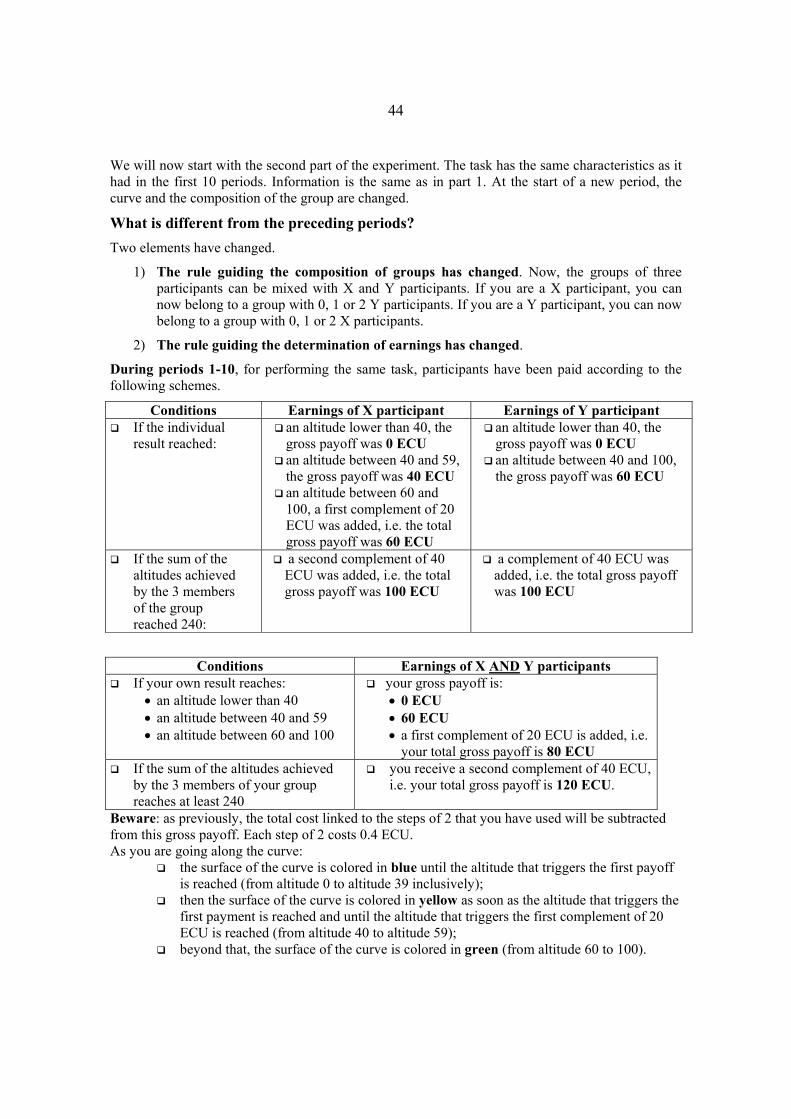
44

We will now start with the second part of the experiment. The task has the same characteristics as it had in the first 10 periods. Information is the same as in part 1. At the start of a new period, the curve and the composition of the group are changed.

What is different from the preceding periods? Two elements have changed.

1) The rule guiding the composition of groups has changed. Now, the groups of three participants can be mixed with X and Y participants. If you are a X participant, you can now belong to a group with 0, 1 or 2 Y participants. If you are a Y participant, you can now belong to a group with 0, 1 or 2 X participants.

2) The rule guiding the determination of earnings has changed.

During periods 1-10, for performing the same task, participants have been paid according to the following schemes.

Conditions Earnings of X participant Earnings of Y participant If the individual

result reached:

an altitude lower than 40, the gross payoff was 0 ECU an altitude between 40 and 59, the gross payoff was 40 ECU an altitude between 60 and 100, a first complement of 20 ECU was added, i.e. the total gross payoff was 60 ECU

an altitude lower than 40, the gross payoff was 0 ECU an altitude between 40 and 100, the gross payoff was 60 ECU

If the sum of the altitudes achieved by the 3 members of the group reached 240:

a second complement of 40 ECU was added, i.e. the total gross payoff was 100 ECU

a complement of 40 ECU was added, i.e. the total gross payoff was 100 ECU

Conditions Earnings of X AND Y participants If your own result reaches:

• an altitude lower than 40 • an altitude between 40 and 59 • an altitude between 60 and 100

your gross payoff is: • 0 ECU • 60 ECU • a first complement of 20 ECU is added, i.e.

your total gross payoff is 80 ECU If the sum of the altitudes achieved

by the 3 members of your group reaches at least 240

you receive a second complement of 40 ECU, i.e. your total gross payoff is 120 ECU.

Beware: as previously, the total cost linked to the steps of 2 that you have used will be subtracted from this gross payoff. Each step of 2 costs 0.4 ECU. As you are going along the curve:

the surface of the curve is colored in blue until the altitude that triggers the first payoff is reached (from altitude 0 to altitude 39 inclusively);

then the surface of the curve is colored in yellow as soon as the altitude that triggers the first payment is reached and until the altitude that triggers the first complement of 20 ECU is reached (from altitude 40 to altitude 59);

beyond that, the surface of the curve is colored in green (from altitude 60 to 100).

45

In other words, as long as the surface of the curve is blue, your gross payoff is null (you may even loose money if you have used steps of 2). As long as the curve is yellow, your gross payoff amounts to 60. When it becomes green, your gross payoff is 80 ECU. And, depending on the cumulated altitude reached by you and the two other members of your group, you will be informed at the end of the period whether you have reached the second complement that yields a total gross payoff of 120 ECU or not.

Instructions for X participants in the fixed-treatment – Part 1

You are going to participate in an experiment about incentives in work organization that is part of a scientific program supported by your company and by the CNRS.

During this experimental session, you can earn money. The amount of your earnings depends not only on your decisions, but also on the decisions of the other participants with whom you will interact.

This session consists in 2 parts of 10 periods each. The session should last about one hour. During this session, transactions are conducted in ECU (Experimental Currency Units). Your final earnings are equal to the sum of the ECU you will earn in each of the 20 periods. At the end of the session, the total amount of ECU you have earned will be converted to Euros at the following rate:

10 ECU = 0.30 €

In addition, you will receive a show-up fee of 7,60 €. Your entire earnings from the experiment will be paid in vouchers that will be given to you in a few days.

Periods 1-10

What does occur in each period? In each period, which lasts 1 minute, each participant has to perform a task on his or her computer.

The task consists in uncovering a curve where a line has been plotted beforehand.

This curve is increasing and/or flat but it never decreases. It can have single or multiple peaks, with a maximum of 3 peaks that are ranked from the lowest to the highest. The highest altitude that can be reached by this curve is 100.

You uncover the line of this curve as you move along. Starting from point 0, you are make progress at the same time in terms of distance (you go along the horizontal axis) and in terms of altitude (you go up on the vertical axis). Time starts running as soon as you click the “OK” button. You can move by clicking one of the two buttons offered on your computer screen. These two buttons correspond to two available speeds.

A first button enables you to take steps of 1. Steps of 1 do not cost money. A second button enables you to take steps of 2. These steps are twice as rapid as steps of 1,

but each step of 2 costs 0.4 ECU. You may switch speed whenever you want and as many times as you like. As long as you do not want to change your speed, you can hold the mouse down and the progression along the curve automatically proceeds at the chosen speed. You can stop your progression whenever you like, even before the one-minute time is over.

46

When a new period starts, you have to uncover a different curve.

With whom do you interact? In each period, you are a member of a team made-up of three people. The other two members of your group have to uncover the same curve as you do on their computer screen but none of you knows the current position or the progression of the two other members of the group. For each new period, the composition of the group is changed.

How are your earnings determined? Your earnings for each period depend on the following elements:

your own result, which corresponds to the altitude reached on the curve when you stop your progression or when the time is over; this means that only altitude matters; distance does not matter;

the result of your group, i.e. the sum of the altitudes reached by each of the three members of your group;

the number of steps of 2 that you made, since these steps cost money. Your earnings are determined as follows:

Conditions Gross payoff If your own outcome reaches: • an altitude lower than 40 • an altitude between 40 and 59 • an altitude between 60 and 100

your gross payoff is: • 0 ECU • 40 ECU • a first complement of 20 ECU is added, i.e.

your gross total payoff is 60 ECU If the sum of the altitudes

achieved by the 3 members of your group reaches at least 240

you receive a second complement of 40 ECU. Your total gross payoff is then 100 ECU.

Beware : the total cost linked to the steps of 2 that you have used will be subtracted from this gross payoff. What information do you receive for each period? During each period, you are informed of the following elements via your computer screen:

the moment when your result has reached the altitudes of 40, 60 and 100

the time remaining

the cumulated cost of steps of 2

In addition, as you are going along the curve: the surface of the curve is colored in blue until the altitude that triggers the first payoff

is reached (from altitude 0 to altitude 39 inclusively); the surface of the curve is colored in yellow as soon as the altitude that triggers the first

payoff is reached and until the altitude that triggers the first complement is reached (from altitude 40 to altitude 59);

beyond that, the surface of the curve is colored in green (from altitude 60 to 100).

47

In other words, as long as the surface of the curve is blue, your gross payoff is null (you may even loose money if you have used steps of 2). When the curve becomes yellow, your gross payoff amounts to 40. When the curve becomes green, your gross payoff is 60 ECU and, depending on the cumulated altitude reached by you and the two other members of your group, you will be informed at the end of the period whether you have reached the second complement that yields a total gross payoff of 100 ECU or not.

At the end of each period, a summary table indicates for each past period:

your final altitude

the cumulated altitude of your group

the total cost of steps of 2 that you used

whether you have reached the first payoff of 40 ECU and the first complement of 20 ECU

whether the cumulated result of your group enables you to get the second complement of 40 ECU

your total net earnings.

*** If you have any questions regarding these instructions, please raise your hand. Someone will answer your questions privately. Throughout the entire session, talking is not allowed. As soon as everybody is ready, we will begin with 3 practice periods, in order for you to familiarize yourself with the task at hand. The results of these practice periods will not be taken into account in your earnings.

Thank you for your participation.

***

Instructions for Y participants in the fixed-treatment – Part 1

You are going to participate in an experiment about incentives in work organization, which is part of a scientific program supported by your company and by the CNRS.

During this experimental session, you can earn money. The amount of your earnings depends not only on your decisions, but also on the decisions of the other participants with whom you will interact.

This session consists in 2 parts of 10 periods each. The session should last about one hour. During this session, transactions are conducted in ECU (Experimental Currency Units). Your final earnings are equal to the sum of the ECU you will earn in each of the 20 periods. At the end of the session, the total amount of ECU you have earned will be converted to Euros at the following rate:

10 ECU = 0.30 €

In addition, you will receive a show-up fee of 7,60 €. Your entire earnings from the experiment will be paid in vouchers that will be given to you in a few days. Periods 1-10

What does occur in each period? In each period, which lasts 1 minute, each participant has to perform a task on his or her computer.

48

The task consists in uncovering a curve where a line has been plotted beforehand. This curve is increasing and/or flat but it never decreases. It can have single or multiple peaks with a maximum of 3 that are ranked from the lowest to the highest. The highest altitude that can be reached by this curve is 100.

You uncover the line of this curve as you move along. Starting from point 0, you make progress at the same time in terms of distance (you go along the horizontal axis) and in terms of altitude (you go up on the vertical axis). Time starts running as soon as you click the “OK” button. You can move by clicking one of the two buttons offered on your computer screen. These two buttons correspond to two available speeds.

A first button enables you to take steps of 1. Steps of 1 do not cost money. A second button enables you to take steps of 2. These steps are twice as rapid as steps of 1,

but each step of 2 costs 0.4 ECU. You may switch speed whenever you want and as many times as you like. As long as you do not want to change your speed, you can hold the mouse down and the progression along the curve automatically proceeds at the chosen speed. You can stop your progression whenever you like, even before the one-minute time is over. When a new period starts, you have to uncover a different curve. With whom do you interact? In each period, you are member of a team made-up of three people.

The other two members of your group have to uncover the same curve as you do on their computer screen but none of you knows the current position or the progression rhythm of the two other members of the group. For each new period, the composition of the group is changed.

How are your earnings determined? Your earnings for each period depend on the following elements:

your own result, which corresponds to the altitude reached on the curve when you stop your progression or when the time is over; this means that only altitude matters; distance does not matter;

the result of your group, i.e. the sum of the altitudes reached by each of the three members of your group;

the number of steps of 2 that you made, since these steps cost money. Your earnings are determined as follows:

Conditions Gross payoff If your own result reaches:

• an altitude lower than 40 • an altitude between 40 and 100

your gross payoff is: • 0 ECU • 60 ECU

If the sum of the altitudes achieved by the 3 members of your group reaches at least 240

you receive a complement of 40 ECU. Your total gross payoff is then 100 ECU.

Beware: the total cost linked to the steps of 2 that you have used will be subtracted from this gross payoff.

49

Which information do you receive for each period? During each period, you are informed of the following elements via your computer screen:

the moment when your result has reached the altitudes of 40 and 100

the time remaining

the cumulated cost of steps of 2

In addition, as you are going along the curve: the surface of the curve is colored in blue until the altitude that triggers the first payoff

is reached (from altitude 0 to altitude 39 inclusively); the surface of the curve is colored in yellow as soon as the altitude that triggers the first

payoff is reached (from altitude 40 to altitude 100). In other words, as long as the surface of the curve is blue, your gross payoff is null (you may even loose money if you have used steps of 2). When the curve becomes yellow, your gross payoff amounts to 60 and, depending on the cumulated altitude reached by you and the two other members of your group, you will be informed at the end of the period whether you have reached the complement that yields a total gross payoff of 100 ECU or not.

At the end of each period, a summary table indicates for each past period:

your final altitude

the cumulated altitude of your group

the total cost of steps of 2 that you used

whether you have reached the first payoff of 60 ECU

whether the cumulated result of your group enables you to get the complement of 40 ECU

your total net earnings.

*** If you have any questions regarding these instructions, please raise your hand. Someone will answer your questions privately. Throughout the entire session, talking is not allowed. As soon as everybody is ready, we will begin with 3 practice periods, in order for you to familiarize yourself with the task at hand. The results of these practice periods will not be taken into account in your earnings.

Thank you for your participation.

***

Instructions for both X and Y participants in the fixed-treatment – Part 2

Periods 11 – 20

We will now start with the second part of the experiment. The task has the same characteristics as it had in the first 10 periods. Information is the same as in part 1. At the start of a new period, the curve and the composition of the group are changed.

50

What is different from the preceding periods? Your gross earnings are now determined as follows for each period.

Conditions Gross payoff If your own result reaches:

• an altitude lower than 40 • an altitude between 40 and 59 • an altitude between 60 and 100

your gross payoff is: • 0 ECU • 60 ECU • a first complement of 20 ECU is added, i.e.

your total gross payoff is 80 ECU If the sum of the altitudes achieved

by the 3 members of your group reaches at least 240

you receive a second complement of 40 ECU, i.e. your total gross payoff is 120 ECU.

Beware: as previously, the total cost linked to the steps of 2 that you have used will be subtracted from this gross payoff. Each step of 2 still costs 0.4 ECU. As you are going along the curve:

the surface of the curve is colored in blue until the altitude that triggers the first payoff is reached (from altitude 0 to altitude 39 inclusively);

then the surface of the curve is colored in yellow as soon as the altitude that triggers the first payment is reached and until the altitude that triggers the first complement of 20 ECU is reached (from altitude 40 to altitude 59);

beyond that, the surface of the curve is colored in green (from altitude 60 to 100). In other words, as long as the surface of the curve is blue, your gross payoff is null (you may even loose money if you have used steps of 2). As long as the curve is yellow, your gross payoff amounts to 60. When it becomes green, your gross payoff is 80 ECU. And, depending on the cumulated altitude reached by you and the two other members of your group, you will be informed at the end of the period whether you have reached the second complement that yields a total gross payoff of 120 ECU or not.