REDESIGN OF DATABASE ALGORITHMS

FOR NEXT GENERATION

NON-VOLATILE MEMORY TECHNOLOGY

Weiwei Hu

Bachelor of Engineering

Tsinghua University, China

A THESIS SUBMITTED

FOR THE DEGREE OF MASTER OF SCIENCE

SCHOOL OF COMPUTING

NATIONAL UNIVERSITY OF SINGAPORE

2012

brought to you by COREView metadata, citation and similar papers at core.ac.uk

provided by ScholarBank@NUS

Acknowledgement

I would like to express my sincere gratitude to my supervisor, Prof. Beng Chin Ooi

for his guidance and encouragement throughout the research work. His continuous

support led me to the right way. He teaches me the right working attitude which

I believe will help me a lot along my whole life. His understanding and guidance

provides me a good direction of my thesis.

I would also like to thank Prof. Kian-Lee Tan and Guoliang Li, who help me a

lot to edit the paper and give me valuable advice for research.

During this work I have collaborated with many colleagues in the database lab,

who have given me lots of valuable comments and ideas. I would like to thank

all of them. They are Sai Wu, Su Chen, Vo Hoang Tam, Suraj Pathak, Peng Lu,

Yanyan Shen etc. I have really enjoyed the pleasant cooperation and work with

these smart and motivated people.

Finally, and most importantly, I would like to thank my parents for their encour-

agement and support. All of these have helped me a lot to complete my graduate

studies and this research work.

i

Contents

Acknowledgement i

Summary v

1 Introduction 1

1.1 Our Contributions . . . . . . . . . . . . . . . . . . . . . . . . . . . 3

1.2 Outline of The Thesis . . . . . . . . . . . . . . . . . . . . . . . . . . 4

2 Next-generation Non-volatile Memory Technology 6

2.1 NVM Technology . . . . . . . . . . . . . . . . . . . . . . . . . . . . 6

2.2 Positions in the Memory Hierarchy . . . . . . . . . . . . . . . . . . 9

2.3 Challenges to Algorithms Design . . . . . . . . . . . . . . . . . . . 10

2.4 Algorithms Design Considerations . . . . . . . . . . . . . . . . . . . 12

2.5 Summary . . . . . . . . . . . . . . . . . . . . . . . . . . . . . . . . 13

3 Literature Review 15

3.1 Write-optimized Indexing Algorithms . . . . . . . . . . . . . . . . . 15

3.1.1 HDD-based Indexing . . . . . . . . . . . . . . . . . . . . . . 16

3.1.2 SSD-based Indexing . . . . . . . . . . . . . . . . . . . . . . 18

3.1.3 WORM-based Indexing . . . . . . . . . . . . . . . . . . . . . 20

ii

3.1.4 PCM-based Indexing . . . . . . . . . . . . . . . . . . . . . . 20

3.2 Query Processing Algorithms . . . . . . . . . . . . . . . . . . . . . 21

3.2.1 Adaptive Query Processing . . . . . . . . . . . . . . . . . . 21

3.2.2 SSD-based Query Processing . . . . . . . . . . . . . . . . . . 24

3.3 PCM-based Main Memory System. . . . . . . . . . . . . . . . . . . 26

3.4 Prediction Model . . . . . . . . . . . . . . . . . . . . . . . . . . . . 27

3.5 Summary . . . . . . . . . . . . . . . . . . . . . . . . . . . . . . . . 29

4 Predictive B+-Tree 31

4.1 Overview of the Bp-tree . . . . . . . . . . . . . . . . . . . . . . . . 31

4.1.1 Design Principle . . . . . . . . . . . . . . . . . . . . . . . . . 32

4.1.2 Basic Idea . . . . . . . . . . . . . . . . . . . . . . . . . . . . 33

4.2 Main Components of Bp-tree . . . . . . . . . . . . . . . . . . . . . 34

4.2.1 DRAM Buffer . . . . . . . . . . . . . . . . . . . . . . . . . . 35

4.2.2 Warm-up Phase . . . . . . . . . . . . . . . . . . . . . . . . . 36

4.2.3 Update Phase . . . . . . . . . . . . . . . . . . . . . . . . . . 37

4.3 Summary . . . . . . . . . . . . . . . . . . . . . . . . . . . . . . . . 39

5 Predictive Model 41

5.1 Predictive Model for Warm-up . . . . . . . . . . . . . . . . . . . . . 41

5.1.1 Predicting the Bp-tree Skeleton . . . . . . . . . . . . . . . . 42

5.1.2 Bp-tree Construction . . . . . . . . . . . . . . . . . . . . . 43

5.2 Predictive Model for Updates . . . . . . . . . . . . . . . . . . . . . 48

5.2.1 Search . . . . . . . . . . . . . . . . . . . . . . . . . . . . . . 48

5.2.2 Deletion . . . . . . . . . . . . . . . . . . . . . . . . . . . . . 49

5.2.3 Insertion . . . . . . . . . . . . . . . . . . . . . . . . . . . . . 50

iii

5.3 Evaluating Bp-tree . . . . . . . . . . . . . . . . . . . . . . . . . . . 53

5.4 Summary . . . . . . . . . . . . . . . . . . . . . . . . . . . . . . . . 56

6 Experimental Evaluation 57

6.1 Experimental Setup . . . . . . . . . . . . . . . . . . . . . . . . . . . 57

6.1.1 Experimental platform . . . . . . . . . . . . . . . . . . . . . 58

6.1.2 Data sets and workloads . . . . . . . . . . . . . . . . . . . . 58

6.1.3 Algorithms compared . . . . . . . . . . . . . . . . . . . . . . 59

6.2 Results and Analysis . . . . . . . . . . . . . . . . . . . . . . . . . . 60

6.2.1 Insertion . . . . . . . . . . . . . . . . . . . . . . . . . . . . . 60

6.2.2 Update . . . . . . . . . . . . . . . . . . . . . . . . . . . . . . 62

6.2.3 Search . . . . . . . . . . . . . . . . . . . . . . . . . . . . . . 63

6.2.4 Node Utilization . . . . . . . . . . . . . . . . . . . . . . . . 65

6.2.5 Sensitivity to Data Distribution Changes . . . . . . . . . . . 66

6.3 Summary . . . . . . . . . . . . . . . . . . . . . . . . . . . . . . . . 67

7 Conclusion 70

7.1 Conclusion . . . . . . . . . . . . . . . . . . . . . . . . . . . . . . . . 70

7.2 Future Work . . . . . . . . . . . . . . . . . . . . . . . . . . . . . . . 71

iv

Summary

In recent years, non-volatile memory like PCM has been considered an attractive

alternative to flash memory and DRAM. It has promising features, including non-

volatile storage, byte addressability, fast read and write operations, and supports

random accesses. Many research scholars are working on designing adaptive sys-

tems based on such memory technologies. However, there are also some challenges

in designing algorithms for this kind of non-volatile-based memory systems, such

as longer write latency and higher energy consumption compared to DRAM. In

this thesis, we will talk about our redesign of the indexing technique for traditional

database systems for them.

We propose a new predictive B+-tree index, called the Bp-tree. which is tailored

for database systems that make use of PCM. We know that the relative slow-write

is one of the major challenges when designing algorithms for the new systems and

thus our trivial target is to avoid the writes as many as possible during the execution

of our algorithms. For B+-tree, we find that each time a node is full, we need to

split the node and write half of the keys on this node to a new place which is the

major source of the more writes during the construction of the tree. Our Bp-tree can

reduce the data movements caused by tree node splits and merges that arise from

insertions and deletions. This is achieved by pre-allocating space on the memory

v

for near future data. To ensure the space are allocated where they are needed, we

propose a novel predictive model to ascertain future data distribution based on the

current data. In addition, as in [6], when keys are inserted into a leaf node, they

are packed but need not be in sorted order which can also reduce some writes.

We implemented the Bp-tree in PostgreSQL and evaluated it in an emulated

environment. Since we do not have any PCM product now, we need to simulate

the environment in our experiments. We customized the buffer management and

calculate the number of writes based on the cache line size. Besides the normal

insertion, deletion and search performance, we also did experiments to see how

sensitive our Bp-tree is to the changes of the data distribution. Our experimental

results show that the Bp-tree significantly reduces the number of writes, therefore

making it write and energy efficient and suitable for a PCM-like hardware environ-

ment. For the future work, besides the indexing technique, we can move on to make

the query processing more friendly to the next generation non-volatile memory.

vi

List of Tables

2.1 Comparison of Memory Technologies . . . . . . . . . . . . . . . . . 8

4.1 Notations . . . . . . . . . . . . . . . . . . . . . . . . . . . . . . . . 35

6.1 Parameters and their value ranges . . . . . . . . . . . . . . . . . . . 59

vii

List of Figures

2.1 PCM Technology . . . . . . . . . . . . . . . . . . . . . . . . . . . . 7

2.2 PCM Usage Proposals . . . . . . . . . . . . . . . . . . . . . . . . . 10

4.1 Bp-tree architecture . . . . . . . . . . . . . . . . . . . . . . . . . . . 35

4.2 An example of a warm-up phase . . . . . . . . . . . . . . . . . . . . 37

4.3 An example for update phase . . . . . . . . . . . . . . . . . . . . . 38

5.1 Warmup Algorithm . . . . . . . . . . . . . . . . . . . . . . . . . . . 47

5.2 Bp-tree: Search Operation . . . . . . . . . . . . . . . . . . . . . . . 49

5.3 Bp-tree: Deletion Operation . . . . . . . . . . . . . . . . . . . . . . 50

5.4 Bp-tree: Insertion Operation . . . . . . . . . . . . . . . . . . . . . . 54

6.1 Insertion performance . . . . . . . . . . . . . . . . . . . . . . . . . . 61

6.2 Update performance . . . . . . . . . . . . . . . . . . . . . . . . . . 64

6.3 Search performance . . . . . . . . . . . . . . . . . . . . . . . . . . . 64

6.4 Leaf nodes utilization . . . . . . . . . . . . . . . . . . . . . . . . . . 66

6.5 Sensitivity to Data Distribution Changes . . . . . . . . . . . . . . . 68

viii

Chapter 1

Introduction

In the established memory technologies hierarchy, DRAMs and flash memories are

two major types that are currently in use, but both of them suffer from vari-

ous shortcomings: DRAMs are volatile and flash memories exhibit limited write

endurance and low write speed. In recent years, we found that the emerging next-

generation non-volatile memory (NVM) is a promising alternative to the traditional

flash memory and DRAM as it offers a combination of some of the best features of

both types of traditional memory technologies. In the near future NVM is expected

to become a common component of the memory and storage technology hierarchy

for PCs and servers [8, 14, 27].

In this thesis, we will research on how to make the emerging next-generation

non-volatile memory adaptive to the existing memory system hierarchy. In partic-

ular, we will focus on how to make the traditional database systems work efficiently

on the NVM-based memory systems. The problem becomes how should the tra-

ditional database systems be modified to best make use of the NVM? This thesis

is an initial research on this topic and we will present our design for the indexing

1

technique. In the future, we can continue to work on redesigning many other com-

ponents in database systems including query processing, buffer management and

transaction management etc.

There are some widely pursued NVM technologies: magneto-resistive random

access memory (MRAM), ferroelectric random access memories (FeRAM), resis-

tive random access memory (RRAM),spin-transfer torque memory (STT-RAM),

and phase change memory (PCM)[17] and in this thesis, we will focus on PCM

technology since it is at a more advanced stage of development and our algorithms

can be adapted to other similar memory technologies. We know that there are some

differences among the different kinds of NVM technologies, but in the remainder of

this thesis, we will use PCM and NVM interchangeably for simplicity and mainly

focus on the PCM technology.

Like DRAM, PCM is byte addressable and supports random accesses. Howev-

er, PCM is non-volatile and offers superior density to DRAM and thus provides

a much larger capacity within the same budget [27]. Compared to NAND flash,

PCM offers better read and write latency, better endurance and lower energy con-

sumption. Based on these features, PCM can be seen as a form of middleware

between DRAM and NAND flash, and we can expect it to have a big impact on

the memory hierarchy. Due to its attractive attributes, PCM has been considered

a feasible device for database systems [27, 6]. In this thesis, we focus on designing

indexing techniques in PCM-based hybrid main memory systems, since indexing

will greatly influence the efficiency of the traditional database systems.

There are several main challenges in designing new algorithms for PCM. First,

though PCM is faster than NAND flash, it is still much slower than DRAM, es-

pecially the write function, which greatly affects system performance. Second, the

2

PCM device consumes more energy because of the phase change of the material.

We will elaborate on this point in Chapter 2. Third, compared to DRAM, the

lifetime of PCM is shorter, which may limit the usefulness of PCM for commercial

systems. However, as mentioned in [27, 6], some measures could be taken to reduce

write traffic as a means to extend the overall lifetime. This, however, may require

substantial redesigning of the whole database system. In general, the longer access

latency and the higher energy consumption are the major factors that affect the

performance of PCM-based memory systems.

1.1 Our Contributions

In this thesis, we propose the predictive B+-tree (called Bp-tree), an adaptive in-

dexing structure for PCM-based memory. Our main objective is to devise new

algorithms to reduce the number of writes without sacrificing the search efficiency.

Our Bp-tree is able to achieve much higher overall system performance than the

classical B+-tree in the PCM-based systems. To the best of our knowledge, no

paper has addressed the issue in such detail and thoroughness. To summarize, we

make the following contributions:

1. We first look into the technology details of the next generation non-volatile

memory technology and then we conduct a comprehensive literature review

about the indexing design in the traditional database systems which can con-

tribute to our redesign. We also showed the algorithms design consideration

for the NVM-based systems.

2. We propose a new predictive B+-tree index, called the Bp-tree, which is de-

signed to accommodate the features of the PCM chip to allow it to work

3

efficiently in PCM-based main memory systems. The Bp-tree can significant-

ly reduce both number of writes and energy consumption.

3. We implemented the Bp-tree in the open source database system PostgreSQL1,

and run it in an emulated environment. Via these experiments, we will show

that our new Bp-tree index significantly outperforms the typical B+-tree in

terms of insertion and search performance and energy consumption.

1.2 Outline of The Thesis

The remainder of the thesis is organized as follows:

• Chapter 2 introduces the next generation non-volatile memory technology.

We provides the technical specifications of some NVM technology and do a

comparison between the existing memory technologies and NVM. Based on

the understanding of the technical specifications, we present our consideration

about how to design adaptive algorithms for NVM-based database systems.

• Chapter 3 reviews the existing related work. In this chapter, we did a com-

prehensive literature review about the write optimized tree indexing and the

existing redesigning work of the NVM-based memory systems. Besides, we

also reviewed the existing proposals about the query processing techniques

which can be referenced in our future work.

• Chapter 4 presents the Bp-tree. In this chapter, we propose the main design

of Bp-tree. We talked about the major structure of the tree and gave the

algorithms about how to insert and search keys on our Bp-tree.

1http://www.postgresql.org/

4

• Chapter 5 presents a predictive model to perform the predicting of future

data distribution. In the previous chapter, we have present that we need a

predictive model to predict the future data distribution and in this chapter,

we present the details of our predictive model and show how to integrate the

predictive model into our Bp-tree.

• Chapter 6 presents the experimental evaluation. In this chapter, we did

various experiments in our simulation environment and showed that our Bp-

tree reduces both execution time and energy consumption.

• Chapter 7 concludes the paper and provide a future research direction. In

this chapter, we concluded our work on the indexing technique and gave some

direction of the future work. We can continue to work on many other com-

ponents of database systems including query processing, buffer management

and transaction management etc.

5

Chapter 2

Next-generation Non-volatile

Memory Technology

Research work on next-generation non-volatile memory technology has grown rapid-

ly in recent years. Worldwide research and development effort have been made on

the emerging new memory devices [38]. Before we move on to what we have done

for the new design, we need to be clear about what exactly this emerging new

memory technology is. In this chapter, we will review the technical specifications

about the PCM technology. Besides, we will also talk about the challenges we face

to design algorithms for such systems and further our design considerations and

targets.

2.1 NVM Technology

There are some widely pursued NVM technologies: magneto-resistive random ac-

cess memory (MRAM), ferroelectric random access memories (FeRAM), resistive

random access memory (RRAM), spin-transfer torque memory (STT-RAM), and

6

Figure 2.1: PCM Technology

phase change memory (PCM). As they have relatively similar features, in this work

we focus on PCM since it is at a more advanced stage of development and it can

be expected to come out earlier.

Generally, NVM technologies share some features in common. Most NVM chips

have comparable read latency than DRAM and rather higher write latency. They

have lower energy consumption but have limited endurance. Next we will review

the technology details of PCM technology. The physical technology of other NVMs

may be different, but in this work, this is not our major focus and we will mainly

discuss about the PCM technology. Since they share some of the common features,

our design for PCM can be reused for other NVMs.

PCM is a non-volatile memory that exploits the property of some phase change

materials. The phase change material is one type of chalcogenide glass, such as

Ge2Sb2Te5 (GST) and it can be switched between two states, amorphous and crys-

talline by the current injection and the heating element. For a large number of

times, the difference in resistivity is typically about five orders of magnitude [31],

which can be used to represent the two logical states of binary data. As we can see in

Figure 2.1[38], crystallizing the phase change material by heating it above the crys-

7

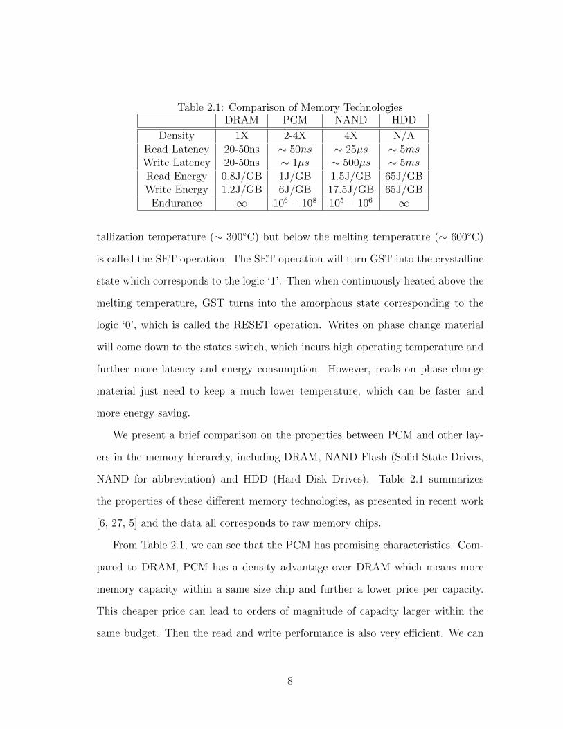
Table 2.1: Comparison of Memory TechnologiesDRAM PCM NAND HDD

Density 1X 2-4X 4X N/ARead Latency 20-50ns ∼ 50ns ∼ 25µs ∼ 5msWrite Latency 20-50ns ∼ 1µs ∼ 500µs ∼ 5msRead Energy 0.8J/GB 1J/GB 1.5J/GB 65J/GBWrite Energy 1.2J/GB 6J/GB 17.5J/GB 65J/GB

Endurance ∞ 106 − 108 105 − 106 ∞

tallization temperature (∼ 300◦C) but below the melting temperature (∼ 600◦C)

is called the SET operation. The SET operation will turn GST into the crystalline

state which corresponds to the logic ‘1’. Then when continuously heated above the

melting temperature, GST turns into the amorphous state corresponding to the

logic ‘0’, which is called the RESET operation. Writes on phase change material

will come down to the states switch, which incurs high operating temperature and

further more latency and energy consumption. However, reads on phase change

material just need to keep a much lower temperature, which can be faster and

more energy saving.

We present a brief comparison on the properties between PCM and other lay-

ers in the memory hierarchy, including DRAM, NAND Flash (Solid State Drives,

NAND for abbreviation) and HDD (Hard Disk Drives). Table 2.1 summarizes

the properties of these different memory technologies, as presented in recent work

[6, 27, 5] and the data all corresponds to raw memory chips.

From Table 2.1, we can see that the PCM has promising characteristics. Com-

pared to DRAM, PCM has a density advantage over DRAM which means more

memory capacity within a same size chip and further a lower price per capacity.

This cheaper price can lead to orders of magnitude of capacity larger within the

same budget. Then the read and write performance is also very efficient. We can

8

see that the read latency of PCM is comparable to that of the DRAM. Although

writes are almost an order of magnitude slower than that of DRAM, some tech-

niques like buffer organization or partial writes could be used in algorithms design

to reduce the performance gap. For NAND, the write on NAND should be based

on pages and even though only small parts of a page are modified, the whole page

need to be rewritten, which is called the erase-before-writes problem. NAND suf-

fers from the erase-before-writes problem greatly and this issue caused the slow

read and write speed directly compared to DRAM and PCM. Unlike NAND, PCM

uses a totally different technology and it does not have the problem of erase-before-

writes and thus supports random reads and writes more efficiently. We can see that

reads and writes on PCM are orders of magnitude faster than those of NAND and

the endurance is also higher than that of NAND. In summary, in most aspects,

PCM can be seen as a technology in the middle between DRAM and NAND Flash.

Even though PCM has its own shortcomings but we believe that it will have a

major role to play in the memory hierarchy, impacting system performance, energy

consumption and reliability because of its promising features.

2.2 Positions in the Memory Hierarchy

In previous section, we talked about the technical specifications of the PCM tech-

nology and we did a comparison between the several commonly used memory tech-

nologies. Now in this section, we want to talk about how to best integrate PCM

into the existing memory systems, in other words, what is the proper position of

PCM in the current memory hierarchy.

In recent years, the computer systems community has already got various re-

9

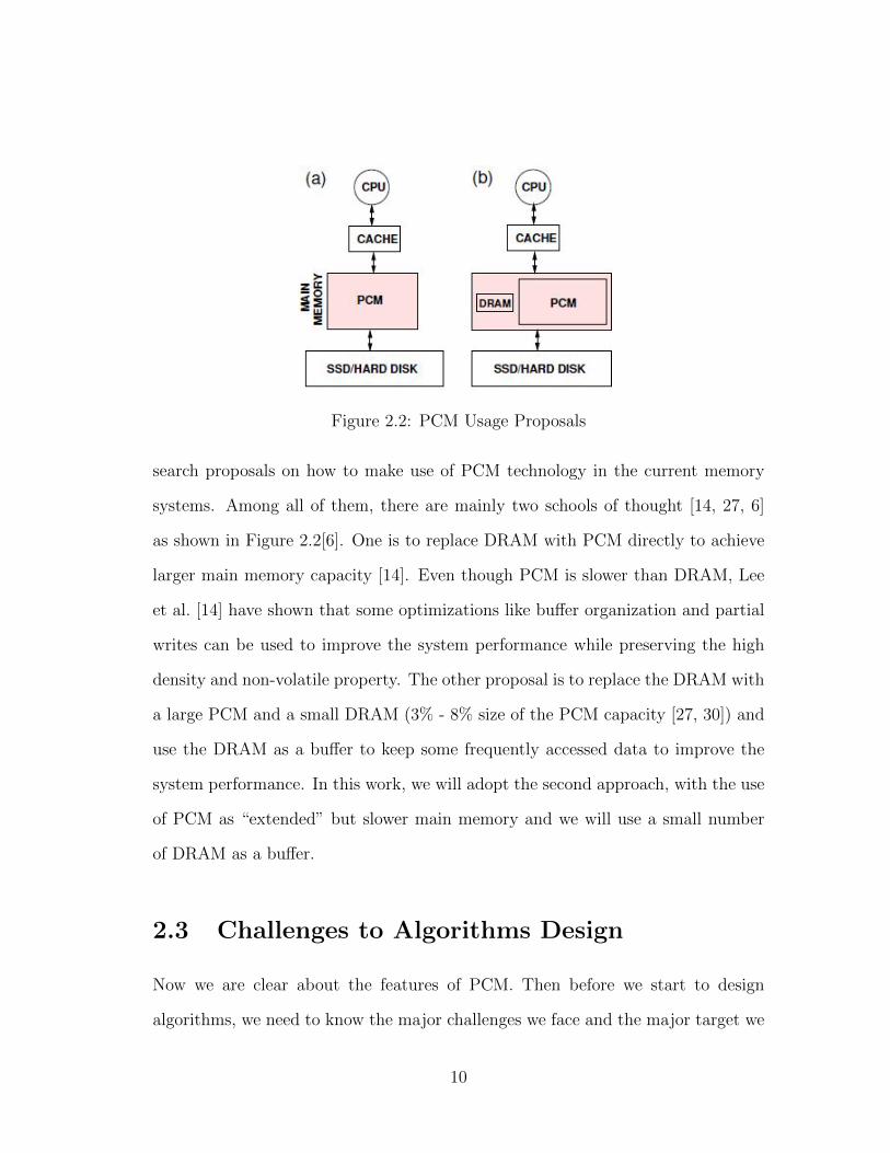
Figure 2.2: PCM Usage Proposals

search proposals on how to make use of PCM technology in the current memory

systems. Among all of them, there are mainly two schools of thought [14, 27, 6]

as shown in Figure 2.2[6]. One is to replace DRAM with PCM directly to achieve

larger main memory capacity [14]. Even though PCM is slower than DRAM, Lee

et al. [14] have shown that some optimizations like buffer organization and partial

writes can be used to improve the system performance while preserving the high

density and non-volatile property. The other proposal is to replace the DRAM with

a large PCM and a small DRAM (3% - 8% size of the PCM capacity [27, 30]) and

use the DRAM as a buffer to keep some frequently accessed data to improve the

system performance. In this work, we will adopt the second approach, with the use

of PCM as “extended” but slower main memory and we will use a small number

of DRAM as a buffer.

2.3 Challenges to Algorithms Design

Now we are clear about the features of PCM. Then before we start to design

algorithms, we need to know the major challenges we face and the major target we

10

want to reach.

From the technologies comparison in previous sections, we can find the following

three challenges we need to overcome.

1. Slow writes. Even the read and write speed is much faster than that of the

NAND, it is still a bit slower than DRAM which will influence the system

efficiency greatly. This challenge is the major one we want to overcome in

this thesis. The idea is a bit trivial that since the writes are slow, we want

to avoid writes as many as possible.

2. High energy consumption. This challenge is related to the writes. We know

that each time we want to write values to the PCM chip, we need to switch its

state. Then we need to heat to switch the state of the phase change material

which leads to high energy consumption. But for read, since we do not need

to switch the state, the energy consumption is much lower.

3. Limited endurance. Existing PCM prototypes have a write endurance ranging

from 106 to 108 writes per cell [6]. With some good round robin or write

leveling algorithms, a PCM main memory can last several years working time

[26]. However, such kinds of algorithms should be conducted in the memory

driver layer, which is not our main focus then.

From these challenges, we can find that actually if we want to make best use

of PCM technology in our existing systems, the most important requirement is to

figure out the challenge of high write latency. Our basic idea is that since the speed

can not be raised physically, can we just avoid the writes as many as possible?

Then The design objective becomes how to reduce the number of writes in our

new algorithms which is an widely studied topic, especially the algorithms designed

11

for NAND in recent years. However, our consideration is different from that of the

algorithms design for NAND. For NAND, they want to avoid the erase-before-writes

and thus they will mostly use the batch algorithms to convert random accesses

to sequential writes. Our design consideration is different that we can support

random writes efficiently but we want to reduce the number of writes including

both random writes and sequential write as many as possible. Once the number of

writes is limited, we can reduce the energy consumption and extend the life time

as well.

2.4 Algorithms Design Considerations

Let us go back to our initial problem that we want to make best use of PCM in

the existing database systems and we want to integrate PCM into the memory

systems. Thus we considering the algorithms design, we need to be careful about

the following design goals: (1) CPU time, (2) CPU cache performance and (3)

energy consumption. Compared to DRAM, the major shortcoming of PCM is the

high write latency. Then for general algorithms, the slow write speed should not

influence the cache performance, it can only influence the CPU execution time

and energy consumption performance. We also know that the PCM writes incur

much higher energy consumption and is much slower than read. Then the major

challenge we are facing now is how to reduce the number of writes as many as

possible. Actually we have already had this basic direction in mind in previous

sections.

Next the problem comes. We need a matric to measure the number of writes

on the database algorithms level. In other words, we need to determine what

12

granularity of writes we need to use in the algorithms analysis using PCM as the

main memory. Generally when analyzing algorithms for main memory, we need to

consider two granularities including bits and cache lines. For the high level database

systems, we have the buffer management and it is easier to count the number of

cache line based writes. However, in order to simulate the energy consumption, we

need to get the number of writes based on the bits granularity.

Then we can use a mixture of these two metrics. To evaluate the CPU time,

we count the number of writes based on the cache line granularity and to evaluate

the energy consumption, we first compare the new cache line to the old cache line

to get the number of modified bits and get the energy consumption then based

on the bits level. Since we have not got any PCM prototype, we need to build a

simulated environment to evaluate our algorithms. These should be configured in

our simulated environment.

2.5 Summary

In this chapter, we introduced the next-generation non-volatile memory technology.

There are many kinds of popular non-volatile memory technologies and in this work,

we will mainly focus on the phase change memory (PCM), but our algorithms can

also be adaptive to other non-volatile memories having the similar features. We

present the technical specification details of PCM and did a comparison among

PCM and some commonly used memory technologies like DRAM, NAND and HDD

about the major features. We found that PCM has its advantages, but there are

also some challenges we need to overcome when designing algorithms for PCM-

based database systems. Our main design goal is to avoid the slow writes as

13

many as possible, which further can reduce the energy consumption and extend

the lifetime of PCM chips. Finally, we discussed about some metrics to evaluate

our new algorithms.

14

Chapter 3

Literature Review

Database research community has contributed a lot to the algorithms design of the

traditional database systems in the last several decades. Database system is also

very complex and there are many components inside each of which can be worthy

of lots of effort to work on. In this work, we mainly focus on the indexing technique

and query processing algorithms. In this thesis, we have proposed a new design of

B+-tree technique and we will leave the query processing to the future work.

In this chapter, we did the literature review, including the write-optimized

indexing algorithms, traditional query processing algorithms and some recent PCM-

based main memory system proposals. Since our indexing design has a prediction

model, we also reviewed some works on histograms and how to use histograms to

construct the prediction model.

3.1 Write-optimized Indexing Algorithms

In previous chapters we know that our main design goal is to reduce the number of

writes, thus we first did a brief survey of the write-optimized indexing techniques.

15

We want to find out whether these existing techniques can be used to our new

PCM-based systems or not and if they can not be used directly, whether we can

borrow some ideas from them. Actually write-optimized B+-tree index has been an

intensive research topic for more than a decade. In this section, we will review the

write-optimized indexing algorithms for HDD, SSD technologies and their design

consideration is similar to ours, but there are also some differences. For HDD-based

indexing, the proposed solutions are mainly focusing on using some DRAM buffer

to convert small random writes into sequential writes. For SSD-based indexing,

some of the proposed solutions change the major structure of B+-tree and some

solutions add an inner layer using SSD between DRAM and HDD, but their major

design consideration is very similar and they expect to avoid the erase-before-writes

as much as possible and they also expect to convert the small random writes into

sequential writes in some sense.

3.1.1 HDD-based Indexing

For the B+-tree index on hard disks, there are many proposals to optimize the

efficiency of write operations and logarithmic structures have been widely used. In

[21], O’Neil et al. proposed the LSM-tree to maintain a real-time low cost index

for the database systems. LSM-tree (Log-Structured Merge-tree) is a disk-based

data structure and it was designed to support high update rate over an extended

period efficiently. The basic idea of LSM-tree is to use an algorithm to defer

and batch the random index changes to reduce the disk arm movements. Some

smaller components of LSM-tree will be entirely memory resident and the larger

and major components will be disk-based. The smaller components resident in

memory will be used as a buffer to keep the frequently referenced page nodes in the

16

larger components. The insertion to the memory resident component has no I/O

cost and the larger component on disk is optimized for sequential disk access with

nodes 100% full. This optimization is similar to that used in the SB-tree [22]. Both

of them support multi-page reads or writes during a sequential access to any node

level below the root, which can offer high-performance sequential disk access for

long range retrievals. Each time when the smaller component reaches a threshold

size near the maximum allotted, it will be merged into the large components on

the disk. A search on the LSM-tree will search both the smaller components in the

memory and the larger components on the disk. Then LSM-tree is most useful in

applications where index insertion are more than searches, which is just the case

for history tables and log files etc.

In [3], Lars Arge proposed the buffer tree for the optimal I/O efficiency. The

structure of the buffer tree is very similar to that of the traditional B+-tree. The

major difference is that in buffer tree, there is a buffer in the main memory for

each node on the hard disk. When we want to update the tree, the buffer tree

will construct an entry with the inserted key, a time stamp and an indication of

whether the key is to be inserted or deleted and put the entry into the buffer of the

root. When the main memory buffer of the root is full, it will insert the elements in

the buffer downwards to its children and this buffer-emptying process will be done

recursively on internal nodes. The main contribution of the buffer tree is that it is

a simple structure with efficient I/O operations and can be applied to other related

algorithms.

Graefe proposed a new write optimized B+-tree index in [10] based on the idea

of the log-structured file systems [32]. Their proposals make the page migration

more efficient and retain the fine-granularity locking, full concurrency guarantees

17

and fast lookup performance at the same time.

Most of the HDD-based write optimized tree indexing follow the following two

idea. First, most of them want to convert the many random writes to batch se-

quential writes to raise the efficiency; second, a small area of DRAM can be used

as the buffer. For our design, we want to support both random and sequential

writes efficiently, thus we cannot “hold” the random writes to a sequential write.

But the idea of using DRAM as buffer can be used as well. In previous chapters,

we have found out that a small area of DRAM buffer can make our system much

more efficient.

3.1.2 SSD-based Indexing

Recently, there are some proposals on the write-optimized B+-tree index on SSDs

[1][15][39]. The major bottleneck of the B+-tree index for SSDs to overcome is the

rather slower small random writes because of the erase-before-write requirement.

In [39], an efficient B-tree layer (BFTL) was proposed to handle the fine-grained

updates of B-tree index efficiently. BFTL is introduced as a layer between file

systems and FTL and thus there is no need to modify the existing applications.

BFTL is considered as a part of the operating system. BFTL consists of a small

reservation buffer and a node translation table. B+-tree index services call from

the upper-level applications are handled and translated from the file system of

operation system to BFTL and then a block-based calls are sent from BFTL to

FTL to do the operation. When a new record is inserted or updated to the B+-

tree, it will first be temporarily held by the reservation buffer of BFTL and then

flushed in batch operation to reduce the writes latency.

FlashDB was proposed in [20] and it is a self-tuning database system optimized

18

for sensor networks using flash SSDs. The self-tuning B+-tree index in the FlashDB

uses two modes, Log and Disk, to make the small random writes together on

consecutive pages. The B+-tree (Disk) assumes that the storage is a disk-like block-

device. The disadvantage is that updates are expensive. Even if only a small part

of the node needs to be updated, the whole block needs to be written. Thus B+-tree

(Disk) is not suitable for write-intensive workload. B+-tree (Log) design is a log-

structured-like indexing and it can avoid the high update cost of B+-tree (Disk).

The basic idea is to construct the index tree as transaction logs. Updates will be

put into buffer first and flushed into SSD when the buffer contains enough data to

fill a page.

More recently, Li et al. [15] proposed the FD-tree which consists of two main

parts, a head B+-tree in the DRAM and several levels of sorted runs in the SSDs.

Thus the basic idea is to limit the random writes to the small top B+-tree and

then merge into the lower runs after they have been transformed into sequential

writes. FD-tree modifies the basic structure of a traditional B+-tree and their major

contribution is to limit random writes to a small area and further raise the insertion

efficiency.

For the SSD-based indexing, some of them tried to use the same idea of that

of the HDD-based indexing. We can adopt the idea of using DRAM as a buffer.

FD-tree is also efficient in some sense, but it modified the basic structure of the B+-

tree, which is not what we want. We want that our B+-tree can be easily adapted

to the existing traditional database systems and thus we do not want to modify

the main structure too much.

19

3.1.3 WORM-based Indexing

There are also some proposals focusing on the Write-Once-Read-Many (WORM)

storage [16][25]. In [16], Mitra, Hsu and Winslett proposed a novel efficient trust-

worthy inverted index for keyword-based search and a secure jump index structure

for multi-keyword searches. In [25], Pei et al. proposed the TS-Trees and they also

built the tree structure based on a probabilistic method. These WORM indexing

proposals mainly focused on designing mechanisms to detect adversarial changes to

guarantee trustworthy search. Unlike WORM indexing, in PCM-based indexing,

we want to reduce the number of writes. Moreover, we can update the index and

afford the small penalty of adjustments due to data movement if the prediction is

no longer that accurate because of changes in data distributions over time.

3.1.4 PCM-based Indexing

The recent study [6] has outlined new database algorithm design considerations for

PCM technology and initiated the research on algorithms for PCM-based database

systems. To our best knowledge, this paper is the most relevant to our work until

now. In the paper, Chen, Gibbons and Nath described the basic characteristics

and the potential impact of PCM on the database system design. They presented

analytic metrics for PCM endurance, energy and latency, and proposed techniques

to modify the current B+-tree index and Hash Joins for better efficiency on the

PCM-based database system. Their idea is to unsort the keys in the node of B+-

tree which can reduce large number of writes. In our proposal, we will take a step

further in this direction and design a PCM-aware B+-tree, called the Bp-tree and

and will compare our Bp-tree with their B+-tree.

20

3.2 Query Processing Algorithms

Query processing is an important part of the traditional database systems. The aim

of query processing is to transform a query in a high-level declarative language (e.g.

SQL) into a correct and efficient execution strategy. Different execution strategies

can lead to much difference in execution efficiency. The traditional query processing

algorithms include two types, one is heuristic-based query optimization and the

other is cost-based query optimization. In heuristic-based query optimization, given

a query expression, the algorithm will perform selections and projections as early

as possible and it will try to eliminate duplicate computations. In cost-based query

optimization, the algorithm will estimate the cost of different equivalent query

calculator and choose the execution plan with the lowest cost estimation.

In this section, we will review the existing query processing algorithms. We

mainly focus on two parts, the adaptive query processing and the recently proposed

query processing for SSD-based database systems. This section of review will give

us some inspiration about what to do in the future and we will discuss about it in

detail in Chapter 7.

3.2.1 Adaptive Query Processing

In traditional query processing, the query optimizer can not have necessary statis-

tics during the compile time, thus it may lead to poor performance, especially in

long running query evaluations. Adaptive query processing addresses this problem

and the idea is to adapt the query plan to changing the environmental conditions at

runtime. In [12], adaptive query processing is defined as that if the query process-

ing system receives information from its environment and determines its behavior

21

according to the information in an iterative manner, that means there is a feedback

loop between the environment and the behavior of the query processing system.

The research on adaptive query processing mainly lies on two main directions. One

is to modify the execution plan at runtime according to the changes of the evalu-

ation environment, the other is to develop new operators that has more flexibility

to deal with unpredictable conditions. Then we will review some of the classical

proposals on adaptive query processing.

Memory Adaptive Sorting and Hash Join

Memory shortage is a common design restriction for query processing techniques,

especially for sorting and join since they need large amount of excess memory.

In [24], Pang et al. introduces new techniques for external sorting to adapt to

fluctuations in memory availability. Since memory buffer size can greatly influence

the performance of sorting, memory-friendly management strategies need to be

taken. [24] introduces a dynamic splitting technique, which adjusts the buffer size

to reduce the performance penalty due to the memory shortages. The basic idea is

to split the merge step of sorting run into some smaller sub-steps in case of memory

shortages and when the memory buffer is larger, it will combine some small sub-

steps into larger steps. This adjust is adaptive and is balancing well. For hash

join, [23] proposes partially preemptible hash joins (PPHJs) which is one kind of

memory adaptive hash joins. The idea is similar to that of [24], they split the

original relations and if the memory buffer is not enough, it will flush part of the

partition to disk. The most efficient case for PPHJs is when the inner relation can

be put in memory but the outer relation can only be scanned and partially put

into the buffer. It can reduce both I/O and the total response time. [40] is also a

22

memory-adaptive sorting which is complementary to [24]. It allows many sorts to

run concurrently to improve the throughput, while [24] focuses on improving the

query response time.

Operators for Producing Partial Results Quickly

In most database applications, we focus on the total response time of all the results.

But in some applications especially in online aggregation, it is important to get

some of the results in a very short time and respond earlier while leaving the

remaining process running at the same time. To this end, pipelining algorithms

are used for the implementation of join and sort operators. Ripple joins [11] are

a new family of physical pipelining join operators. They make use of both block

nested loops join and hash joins. They target on online processing of multi-table

aggregation queries in traditional DBMS. It is designed to minimize the time until

an acceptably precise estimate of the query result is available, as measured by the

length of a confidence interval. Ripple join comes from the nested loops join since

it has an outer relation and an inner relation, the difference is that it adjusts the

retrieve rates of tuples from these two input based on the statistical information

during the runtime and reduce the response time of important part of the whole

results. Xjoin [37] is a variant of Ripple joins. It partitions the input and thus

requires less external memory, which makes it more suitable for parallel processing.

[29] proposes another pipelining reorder operator for providing user control during

long running, data intensive operations to get partial results during the process.

The input of this operator is an unordered set of data and it can produce a nearly

sorted result according to user preferences which can change during the runtime

with an attempt to ensure that interesting items are processed first.

23

Algorithms that Defer Some Optimization Decisions until Runtime

Sometimes the statistical information gathered in the beginning of the query pro-

cessing is not that accurate which can lead to a bad performance. There are some

algorithms that defer some optimization decisions until they have collected enough

statistics. [13] proposes an algorithm that detects sub-optimality in query plans at

runtime, through on-the-fly collection of query statistics. It can improve the total

performance by either reallocating resources (e.g. memory) or by reordering the

query plan. It introduces a new operator called statistics collector operator which

is used for the re-optimization algorithm. The algorithm is heuristics-based and

relies heavily on intermediate data materialization. The new operator is inserted

into the query plan, ensuring that it does not slow down the query by more than

a specific fraction and also assigns a potential inaccuracy level of low, medium or

high to the various estimates, which will be used in the following processing.

3.2.2 SSD-based Query Processing

Recently there are some research work on query processing for SSD-based database

systems. In previous Section 3.1.2, we have said that the major design goal of SSD-

related algorithms is to reduce the influence of the high write latency caused by the

erase-before-write restriction. We will then review the following several proposals

about query processing algorithms.

In [36], Graefe et al. focus on the impact of SSD characteristics on query

processing in relational databases and especially on join processing. They first

demonstrate a column-based layout within each page and show that it can reduce

the amount of data read during selections and projections. Then they introduce

24

FlashJoin, which is a general pipelined join algorithm that minimized accesses to

base and intermediate relational data. FlashJoin has better performance than a

variety of existing binary joins, mainly due to its novel combination of three well-

known ideas: using a column-based layout when possible, creating a temporary

join index and using late materialization to retrieve the non-join attributes from

the fewest possible rows. Then we focus on the details of FlashJoin algorithm.

FlashJoin is a multi-way equi-join algorithm, implemented as a pipeline of stylized

binary joins, each of which includes a join kernel and a fetch kernel. The join kernel

computes the join and outputs a join index, which is used in the fetch kernel to

do a late materialization, which only retrieves the needed attributes to compute

the next join using RIDs specified in the previous join index. The final fetch

kernel retrieves the remaining attributes for the result. The experiments show that

FlashJoin significantly reduces memory and I/O requirements for each join in the

query and raises the query performance greatly.

[35] propose RARE-join algorithm. They convert traditional sequential I/O

algorithms to ones that use a mixture of sequential and random I/O to process

less data in less time. To make scans and projection faster, they examine a PAX-

based page layout [2], which arranges rows within a page in column-major order.

Then they designed the RARE-join (RAndom Read Efficient Join) algorithm for

the column-based page layout. RARE-join first constructs a join index and then

retrieves only the pages and columns needed for computing the join result. The

main idea of RARE-join is very similar to that of the FlashJoin. In [4], the authors

show that many of the results from magnetic HDD-based join methods also hold

for flash SSDs. Their results show that in many cases the block nested loops join

over sort-merge join and grace hash join works well for SSD and they also propose

25

the idea that simply looking at the I/O costs when designing new flash SSD join

algorithms can be problematic, because the CPU cost can be a big part of the total

join cost in some cases. Their idea also tells us that we need to do a precise research

on the new algorithms design and we need to consider all kinds of costs which can

influence the main system performance in different aspects.

3.3 PCM-based Main Memory System.

Several recent studies from the computer architecture community have proposed

new memory system designs on PCM. They mainly focused on how to make PCM

a replacement or an addition to the DRAM in the main memory system. Al-

though these studies mainly focused on the hardware design, they provided us the

motivation on the use of PCM in the new memory hierarchy design for database

applications.

The major disadvantages of the PCM for a main memory system are the limited

PCM endurance, longer access latency and higher dynamic power compared to the

DRAM. There are many relevant studies addressing these problems [27, 41, 14, 26].

In [27], Qureshi, Srinivasan and Rivers designed a PCM-based hybrid main memory

system consisting of the PCM storage coupled with a small DRAM buffer. Such an

architecture has both the latency benefits of DRAM and the capacity benefits of

PCM. The techniques of partial writes, row shifting and segment swapping for wear

leveling to further extend the lifetime of PCM-based systems have been proposed

to reduce redundant bit-writes [41, 14]. Qureshi et al. [26] proposed the Start-

Gap wear-leveling technique and analyzed the security vulnerabilities caused by

the limited write endurance problems. Their proposal requires less than 8 bytes of

26

total storage overhead and increased the achievable lifetime of the baseline system

from 5% to 50% of the theoretical maximum. Zhou et al. [41] also focused on

the energy efficiency and their results indicated that it is feasible to use PCM

technology in place of DRAM in the main memory for better energy efficiency.

There are other PCM related studies such as, [33] focusing on error corrections,

and [34] focusing on malicious wear-outs and durability.

Many of the studies in computer architecture community focus on the lifetime

issue of PCM technology which is in a lower level consideration. This is the reason

why we do not focus on the wear out problem in our proposal. This issue should

be addressed in the PCM driver level and what we want to do is about the upper

level database system algorithms.

3.4 Prediction Model

In this section, we will review the traditional prediction model based on the his-

togram since we need an accurate prediction model in our proposal for indexing

algorithms.

Prediction has always been an extremely important activity and it is an impor-

tant research topic in statistical theory and it is a big business. The basic idea of

prediction is to predict the future value or distribution of a random variable (RV).

The probability distributions of many RVs encountered in practice are subject to

changes over time and thus it is well known that the fundamental goal of predict-

ing is actually to update the probability distribution based on the present and past

information.

Traditionally, we use histogram to represent the distribution of a random vari-

27

able. We divide the observed range of variation of the RV into a number of value

intervals and the relative frequency of each interval is defined to be the proportion

of observed values of the RV that lie in that interval. We define the relative fre-

quency in each value interval Ii is the estimate of the probability pi that the RV

lies in that interval.

Let I1, ..., In be the value intervals with u1, ..., un as their midpoints and p =

(p1, ..., pn) is the probability vector of the distribution of RV. Then we can get µ

and σ as the estimates of expected value µ and standard deviation of the RV.

µ =n∑

i=1

uipi, σ =

√√√√ n∑i=1

pi(ui − u)2 (3.1)

Then we can define the most commonly used probability distribution in deci-

sion making, the normal distribution. It is completely specified by the above two

parameters. It is symmetric around the mean and the probabilities corresponding

to the intervals [µ− σ, µ+ σ], [µ− 2σ, µ+ 2σ], [µ− 3σ, µ+ 3σ] are 0.68, 0.95, 0.997

respectively.

In our prediction model in practice, the probability distributions of RVs may

change with time. For example, the distribution of the values inserted into the B+-

tree may change with time. We want to capture all the dynamic changes occurring

in the shapes of probability distributions from time to time and the traditional

method is not adequate anymore.

In [19], Murty proposes to represent probability distribution by the traditional

distributions to make all changes possible. When updating the distribution of RV,

we can change the values of any pi which makes it possible to capture any change

in the shape of the distribution. In their model, in addition to the present distri-

28

bution vector p1, ..., pn, they add the recent histogram f1, ..., fn and the updated

distribution x1, ..., xn.

f = (f1, ..., fn) represents the estimate of the probability vector in the recent

histogram, but it is based on the most recent few observations (for example 50). p =

(p1, ..., pn) is the probability vector in the traditional distribution at the previous

updating. x = (x1, ..., xn) is the updated probability vector which can be obtained

by incorporating the changing trend reflected in f into p. In [18], the authors

proposed to compute x from p and f using the following formula.

x = βp+ (1− β)f (3.2)

In equation 3.2, β is a weight between 0 and 1 and they found that β =0.8 or

0.9 works well for the model.

We can find that the basic idea of Murty’s proposal is to combine the latest

change trend of the data distribution into the current distribution to better predict

the future distribution. Since they will keep updating the trend vector, the pre-

diction will keep changing based on the current distribution changing trend which

makes the prediction more accurate. Their work may be helpful to our prediction

model to predict the future inserted values into the B+-tree.

3.5 Summary

In this chapter, we did a comprehensive literature review on the related topics to

our problem. Since we want to design a write-optimized indexing technique, we

first reviewed some of the existing write-optimized indexing techniques for other

memory technologies based database systems. Then we reviewed the typical query

29

processing algorithms which can be useful for our future work. After that, we

talked about the recent research proposals on the PCM-based memory systems

design. We have the similar challenges but we are doing the job on a different level

and thus our major focus is a bit different. But some of the basic ideas coming from

the computer architecture community can also be used by our design. Lastly, we

did a brief review about prediction model since we need to use a prediction model

to predict the future database distributions in our design.

30

Chapter 4

Predictive B+-Tree

In previous chapters, we introduced the background information about phase change

memory technology and the algorithms design consideration for PCM-based database

systems. From this chapter, we are going to present the design of our predictive

B+-tree, the Bp-tree. The purpose of our Bp-tree is to reduce the number of writes

of traditional B+-tree while keep the insert and search performance at the same

time. Our basic idea is to reduce the number of node splits caused by being full

since node splits are a major source of the unnecessary writes of keys. As there

are many B+-tree variants in database research community, for simplicity, in our

work, we will use the standard B+-tree and our techniques can be easily extended

to other variants.

4.1 Overview of the Bp-tree

In this section, we will introduce the basic concept of Bp-tree. We first talk about

the design principle of Bp-tree and then we present the basic idea of Bp-tree. The

idea itself is very simple but we need to be very careful to make the tree balance

31

and stable.

4.1.1 Design Principle

Our goal is to reduce the number of writes for data insertions and updates, without

sacrificing the performance of search queries. We have seen that there are many

traditional methods to do write optimization and we can borrow the DRAM buffer

idea. For our own design, we want to reduce the number of writes in the following

two ways. First, we adopt the Unsorted Leaf strategy in [6]. Essentially, newly

inserted keys are simply appended to the end of the key entries. As such, they are

not necessarily in sorted order which may reduce large amount of writes. Hence,

the search cost may incur additional overhead as all entries within a leaf node have

to be examined. But since we now consider the main memory algorithms design

and we want to set the size of the node to several cache lines’ size, this additional

overhead will not be that much. Second, we develop a scheme that minimizes data

movement caused by node splits and merges. We have present in the previous

sections that the splits and merges are the major source of many additional writes

required. If we can reduce the number of splits, the performance can be greatly

raised. But in the traditional B+-tree, the algorithm is very stable that only when

the node is full, the split happens. Or only when the node becomes “underflow”

because of deletion, we merge the sibling nodes. Now we want to reduce these

operations, we need to “break” some of the existing rules. For the remainder of

this thesis, we shall focus on reducing the number of node splits and merges, which

is the main motivation for designing the Bp-tree and we will talk about more details

next.

32

4.1.2 Basic Idea

The general idea is to predict the data distribution based on the past insertions

and pre-allocate space on PCM for accommodating future tree nodes, which can

reduce the key movements caused by node splits and merges. At the same time, it

is possible to fail some of the basic balance properties of B+-tree, but we will adopt

some strategies to ensure the balance property and make sure that the difference

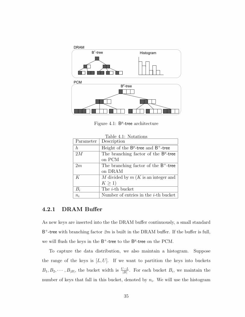
will not influence the performance. Figure 4.1 illustrates the main architecture of

a Bp-tree. We use the following techniques to implement a Bp-tree.

DRAM Buffer

We use a small DRAM buffer to maintain a small B+-tree for current insertions.

We also record the summary of previously inserted keys in a histogram and use

them to predict the structure of the Bp-tree. If the buffer is full, we will merge it

into the Bp-tree on PCM.

Bp-tree on PCM

Like a standard B+-tree, a Bp-tree is also a balanced multiway search tree. The key

differences between the Bp-tree and the B+-tree include:

1. The structures and nodes in a Bp-tree can be pre-allocated.

2. Given a branching factor 2M of a Bp-tree, the number of children of an internal

node may be smaller than M . and the real number of children is between

[0, 2M ].

3. The insertions and deletions are different from the B+-tree (see Section 5.2).

33

4. The tree construction process consists of two phases: (i) warm-up phase:

The first N keys are initially inserted into the tree as a warm-up process; (ii)

update phase: All new keys are first inserted into a DRAM buffer. Each

time the buffer is full, the keys in DRAM would be merged into the main

tree on PCM. For a search query, we will find them from both the B+-tree in

DRAM and the Bp-tree in PCM.

Predictive Model

Predictive model is a very important component in our Bp-tree. Each time we

want to merge the small B+-tree on DRAM to PCM, we need to use the predictive

model. If the model is too sparse, it may lead to many more nodes and the nodes

utilization is very low. If the model is too strict, the influence of the our strategy

may be not that obvious and our Bp-tree becomes similar to the traditional B+-

tree. Thus an accurate predictive model is very important to our design and we

also proposed some strategies to guard the prediction model in order to make it

work properly. Currently in our predictive model, we use the histogram and we

can get better predictive model for better performance in the future.

4.2 Main Components of Bp-tree

In this section, we will describe the details of the construction process of a Bp-tree.

It consists of two phases, namely the warm-up phase and update phase, which will

be described in Section 4.2.2 and Section 4.2.3 respectively.

For ease of presentation, we summarize the notations used throughout this paper

in Table 4.1.

34

PCM

DRAM

Bp-tree

B+-tree Histogram

Figure 4.1: Bp-tree architecture

Table 4.1: NotationsParameter Description

h Height of the Bp-tree and B+-tree2M The branching factor of the Bp-tree

on PCM2m The branching factor of the B+-tree

on DRAMK M divided by m (K is an integer and

K ≥ 1)Bi The i-th bucketni Number of entries in the i-th bucket

4.2.1 DRAM Buffer

As new keys are inserted into the the DRAM buffer continuously, a small standard

B+-tree with branching factor 2m is built in the DRAM buffer. If the buffer is full,

we will flush the keys in the B+-tree to the Bp-tree on the PCM.

To capture the data distribution, we also maintain a histogram. Suppose

the range of the keys is [L,U ]. If we want to partition the keys into buckets

B1, B2, · · · , B|B|, the bucket width is U−L|B| . For each bucket Bi, we maintain the

number of keys that fall in this bucket, denoted by ni. We will use the histogram

35

to “forecast” the data distribution (Section 5.1).

The main function of DRAM buffer is to adaptively adjust our predictive model

based on the currently inserted keys in a time window. Then we can use the updated

predictive model to merge all the keys in the time window in the B+-tree to the

Bp-tree on PCM.

4.2.2 Warm-up Phase

Initially, the Bp-tree on PCM is empty. We use a DRAM buffer for warm-up. We

create a standard B+-tree for supporting insertions, deletions and search. Before

the buffer is full, we use the conventional B+-tree for the initial operations. For the

first time that the DRAM buffer is full, all the keys in the buffer will be moved to

the PCM, and this step is called the warm-up process. The main function of the

warm-up phase is to construct the skeleton of the Bp-tree on PCM.

Suppose the DRAM buffer can accommodate N keys. We first predict the to-

tal number of possible keys. Then, for each B+-tree node, we use our predictive

model to decide whether to split it in an eager manner to avoid writes for subse-

quent insertions. We will provide the details for constructing the initial Bp-tree in

Section 5.1.

Figure 4.2 shows an example for the warm-up phase. The B+-tree and histogram

are in the DRAM and Bp-tree is in the PCM. In this example, N is 10 and the

buffer is full and thus we need to flush all the keys in the B+-tree to the PCM. The

black portion of the histogram bar indicates the number of inserted keys in each

range so far, while the whole bar indicates the predicted number of keys in each

range based on our predictive model. From this figure, we can observe that the

structure of the Bp-tree is similar to that of the original B+-tree. However, there

36

Figure 4.2: An example of a warm-up phase

are two key distinctions. First, the node could be split in an early manner if it

meets the requirement of node splits. Second, some of the nodes could underflow

due to either an enlargement of the node size or an early split. These are guided

by our predictive model and tree construction strategy. In the example, node C

in the B+-tree is split into node C and node C ′ when it is moved to the Bp-tree,

nodes B and E underflow because of the enlargement of the node size, while node

C and node C ′ underflow because of the early split. Details about the early split

algorithm will be presented in Section 5.1.

4.2.3 Update Phase

After the warm-up phase, we have a Bp-tree structure on the PCM. Then for new

operations, we use both the DRAM buffer and Bp-tree to handle the operations.

For an insertion, we insert it into the B+-tree. For a search query, we search the key

37

Figure 4.3: An example for update phase

from both the B+-tree on DRAM and the Bp-tree on PCM. If we find it, we return

the answer; otherwise we return “null”. (Section 5.2.1). For delete, we search it

from both the B+-tree and the Bp-tree. If we find it, we remove it from the B+-

tree and the Bp-tree (Section 5.2.2). However, even if a node “underflows” after

deletions, we do not merge it with its siblings. The reason is that since the read

latency of PCM is much less than the write latency, the overhead caused by empty

nodes during query processing is negligible. Furthermore, space could be reserved

for future insertion keys to reduce subsequent writes. For update operation, like

other indexes, we treat it as a deletion operation followed by an insertion. The

deletion operation does not need to be buffered, while the following insertion needs

to be buffered first like the standard insertion operation on the Bp-tree. Note that

we need to update the histogram for the insertion and deletion operations. If the

DRAM buffer is full, we need to merge the B+-tree into the Bp-tree (Section 5.2.3).

Figure 4.3 shows an example for update phase affected on the earlier example

38

described in Figure 4.2. The case in Figure 4.3 is that the buffer is full for the

second time and all the keys in the B+-tree are merged into the Bp-tree described

in Figure 4.2. In this example for the update phase, we want to delete the key

5 in the Bp-tree index from Figure 4.2. First, we search the B+-tree in the buffer

and cannot find it. Then we search the Bp-tree on the PCM and find it in node

A and subsequently remove it from the Bp-tree. As can be seen from the figure,

the histogram is updated to reflect the effect of this deletion and the new round of

prediction is performed based on all the keys inserted currently including the keys

in the buffer. Node F in the Bp-tree is split because of the similar reason as that

of the node C in Figure 4.2. We will describe the details in Section 5.2.

4.3 Summary

In this chapter, we introduced our Bp-tree. We present the design principle and

basic idea of Bp-tree. We know that there are two major parts of Bp-tree including

the DRAM buffer and the normal B+-tree on PCM. When new keys are inserted

into the Bp-tree, there are two phases. First, the new key is inserted into the small

B+-tree on the DRAM buffer, when the DRAM buffer is full for the first time, we

merge the whole tree to PCM and construct the skeleton of the tree on PCM based

on the predictive model. After that each time when the DRAM is full, we will

merge the tree to the existing B+-tree on PCM. During the construction, the node

of our Bp-tree may be “underflow” which is different from the traditional B+-tree.

The reason is that sometimes we want to split the node in advance based on the

prediction model even the node is not full. In our design, even some nodes may

be “underflow”, we will still use some strategy to ensure that the whole tree is in

39

a good shape. We will talk about the details about the prediction model and the

construction process in next chapter.

40

Chapter 5

Predictive Model

In this chapter, we are going to present the predictive model which is a key part

of our design. In the previous chapter, we have known that there are two major

phases in our Bp-tree, both of which will be based on this predictive model. Thus

in this chapter, we will talk about how we construct the predictive model and use

it in these two phases. We also know that the accuracy of the model is critical

to the performance of the whole indexing and thus we will present our strategy

to evaluate the realtime status of the predictive model and make adjustment to

make it work properly. There will be three major parts of this chapter including

the predictive model for warm-up phase, predictive model for update phase and

evaluating Bp-tree.

5.1 Predictive Model for Warm-up

In this section, we introduce a predictive model to construct a Bp-tree structure

in the warm-up phase. We will present running examples to show what the pre-

dictive model is and how it is integrated into our Bp-tree. We first discuss how to

41

predict a Bp-tree skeleton (Section 5.1.1), and then propose to construct a Bp-tree

(Section 5.1.2).

5.1.1 Predicting the Bp-tree Skeleton

Suppose there are N keys in the DRAM B+-tree, the height of the B+-tree is h, and

the branching factor is 2m. The Bp-tree has the same height as the B+-tree, but

with a larger branching order 2M = K ∗ 2m, where K is an integer and K ≥ 1. K

can be set by the administrator. We can also predict K as follows.

Let T denote the total number of possible keys in the whole dataset. We

estimate T using the numbers of keys in the histogram. Suppose the maximal

number of keys in a bucket is A and the bucket width is W = U−L|B| , thus there are

at most W keys in a bucket. We use N × WA

to predict the possible key number T .

As there are T keys in Bp-tree and N keys in B+-tree, we set K = loghTN

.

Obviously, if we overestimate K, the Bp-tree will turn out to be sparse; on the

contrary, if we underestimate the number, we may need to do more splits. We

assume that each tree node in the final Bp-tree is expected to be µ% full, i.e., each

leaf node has E = µ%× 2M keys. Thus the i-th level is expected to have Ei nodes

(the root is the first level, which has only one node).

After we got the number K, we can build the skeleton of the Bp-tree, in other

words, we are going to enlarge the size of each node in the tree by K, in which case,

there may be many “underflow” nodes. But we will not worry about this and we

will gradually insert keys into these nodes and raise the average node utilization.

42

5.1.2 Bp-tree Construction

In this section, we discuss how to construct the Bp-tree based on the current B+-tree

structure. We traverse the B+-tree in post-order. For each node, we predict whether

we need to split it based on our predictive model (which will be introduced later).

If we need to split it, we split it into two (or more) nodes, and insert separators (or

keys) into its parent node, which may in turn cause the parent node to be split.

Following this approach, the process will continue to spread to the whole tree. As

we employ a post-order traversal, we can guarantee that the child splits are before

the parent split, and our method can keep a balanced tree structure.

Next we discuss how to split a B+-tree node. For ease of presentation, we first

introduce a concept.

Definition 5.1 (Node Extent) Each node n in the index tree is associated with

a key range [nl, nu], where nl and nu are respectively the minimum key and the

maximum key that could fall in this node. We call this range the extent of the

node.

The extent of node A and B of the B+-tree in Figure 4.2, for example, are [0, 19)

and [19, 32) respectively. If a node is not the leftmost or the rightmost child of its

parent, we can get its extent from its parent (except for the root node); otherwise

we need to determine it from its ancestors. In practice, we need to update this

information each time we split or merge nodes and we also need to consider this

overhead in the evaluation.

Consider a B+-tree node n on the i-th level. Suppose its extent is [keymin, keymax]

and currently it has |n| keys, key1, key2, · · · , key|n|. We access the keys in order.

Suppose the current key is keyj. We next discuss whether to split the node ac-

43

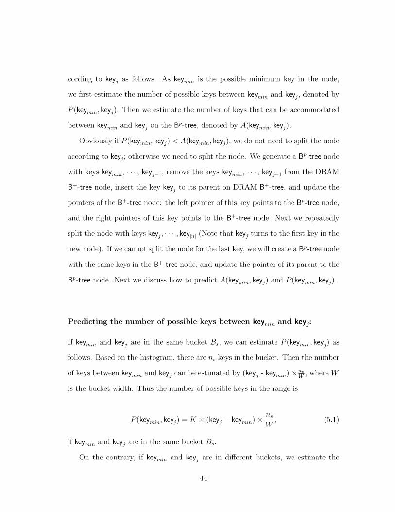
cording to keyj as follows. As keymin is the possible minimum key in the node,

we first estimate the number of possible keys between keymin and keyj, denoted by

P (keymin, keyj). Then we estimate the number of keys that can be accommodated

between keymin and keyj on the Bp-tree, denoted by A(keymin, keyj).

Obviously if P (keymin, keyj) < A(keymin, keyj), we do not need to split the node

according to keyj; otherwise we need to split the node. We generate a Bp-tree node

with keys keymin, · · · , keyj−1, remove the keys keymin, · · · , keyj−1 from the DRAM

B+-tree node, insert the key keyj to its parent on DRAM B+-tree, and update the

pointers of the B+-tree node: the left pointer of this key points to the Bp-tree node,

and the right pointers of this key points to the B+-tree node. Next we repeatedly

split the node with keys keyj, · · · , key|n| (Note that keyj turns to the first key in the

new node). If we cannot split the node for the last key, we will create a Bp-tree node

with the same keys in the B+-tree node, and update the pointer of its parent to the

Bp-tree node. Next we discuss how to predict A(keymin, keyj) and P (keymin, keyj).

Predicting the number of possible keys between keymin and keyj:

If keymin and keyj are in the same bucket Bs, we can estimate P (keymin, keyj) as

follows. Based on the histogram, there are ns keys in the bucket. Then the number

of keys between keymin and keyj can be estimated by (keyj - keymin) ×ns

W, where W

is the bucket width. Thus the number of possible keys in the range is

P (keymin, keyj) = K × (keyj − keymin)× ns

W, (5.1)

if keymin and keyj are in the same bucket Bs.

On the contrary, if keymin and keyj are in different buckets, we estimate the

44

number as follows. Without loss of generality, suppose keymin is in bucket Bs and

keyj is in bucket Be. Let Bus denote the upper bound of keys in bucket Bs and Bl

e

denote the lower bound of keys in bucket Be. Thus the number of keys between

keymin and keyj in bucket Bs is (Bus -keymin) ×ns

W. The number of keys between

keymin and keyj in bucket Be is (keyj - Ble) ×nb

W. Thus the total number of keys

between keymin and keyj is (Bus -keymin) ×ns

W+∑e−1

t=s+1 nt + (keyj - Ble) ×nb

W. Thus

the number of possible keys between keymin and keyj is

P (keymin, keyj) = K ×((Bu

s − keymin)× ns

W+

e−1∑t=s+1

nt + (keyj −Ble)×

nb

W

), (5.2)

if keymin and keyj are in different buckets.

Predicting the number of keys that can be accommodated between keymin

and keyj:

Note that node n has |n| keys and it is expected to have E keys, thus the number

of accommodated keys in this node is E − |n|. Thus

A(keymin, keyj) = min(keyj − keymin, E − |n|),

if n is a leaf node.

If node n is a non-leaf node, we can directly add j children between the two

keys. In addition, we can also add some keys between keymin and keyj as there

are E − |n| positions which are not used in the node. Obviously, we insert at

most min(keyj − keymin, E − |n|) keys in the node. Thus we can add at most

c = j + min(keyj − keymin, E − |n|) children under the node between keymin and

45

keyj. As node n is in the i-level, the children are on i + 1-level. As each child can

have E keys and E + 1 children, each node can have (E + 1)h−i−1 descendants.

Thus there are c×∑h−i−1

t=0 (E + 1)t nodes between the two keys. As each node can

accommodate E keys, the total number of accommodated keys is

A(keymin, keyj) = E × c×h−i−1∑t=0

(E + 1)t, (5.3)

if node n is a non-leaf node.

To summarize, we can use the predicted numbers to split the nodes. Iteratively,

we can split all the nodes and insert the new nodes into PCM. Figure 5.1 illustrates

the algorithm. The Warm-up algorithm first traverses the B+-tree in post-order

by calling its function PostOrder (line 3). Function PostOrder splits the nodes

iteratively. Given a node n on level i, it checks whether the node should be split by

calling function Split (line 4), which is used to split a node based on our predictive

model. If our model decides to split node n, we generate a Bp-tree node with keys,

keymin, · · · , keyj−1 (line 6), remove the keys, keymin, · · · , keyj−1, from the DRAM

B+-tree node (line 7), insert the key keyj to its parent on DRAM B+-tree (line 8),

and update the pointers of the B+-tree node: the left pointer of this key to the

Bp-tree node, and the right pointers of this key to the B+-tree node. Next we

repeatedly split the node with keys, keyj, · · · , key|n| (line 9). If we cannot split the

node for the last key, we will create a Bp-tree node with the keys, and update the

pointer of its parent to the Bp-tree node (line 10). Iteratively, we can construct the

Bp-tree structure.

We show an example of the split algorithms in Figure 4.2. Here we take the leaf

node for an example instead of the whole split algorithm. As can be seen from the

46

Algorithm 1: Warm-up(B+-tree, Histogram)

Input: B+-tree and Histogram in DRAM BufferOutput: Bp-tree on PCMbegin1

Let r denote the root of the B+-tree, Level i = 0 ;2

PostOrder (r, i, Histogram) ;3

end4

Function PostOrder(n, i, Histogram)

Input: n: B+-tree node; i: Level of n; HistogramOutput: Bp-tree nodesbegin1

for each child c of n do2

PostOrder (c, i+ 1, Histogram);3

keyj = Split (n, i, Histogram);4

while keyj ! = φ do5

Generate a Bp-tree node with keymin,· · · ,keyj−1;6

Remove keys after keyj from B+-tree node n;7

Insert keyj to the parent of n on B+-tree and update the pointers ;8

Split(n, i, Histogram);9

Create a node with keymin,· · · ,keyj−1, remove n, update n’s parent;10

end11

Function Split(n, i, Histogram)

Input: n: B+-tree node; i: Level of n; HistogramOutput: Key: Split Keybegin1

Let keymin denote the first key in node n ;2

for j = 2, 3, · · · |n| do3

if PredictTwoKeys (keymin, keyj, i) then4

return keyj ;5

return φ ;6

end7

Function PredictTwoKeys(keymin, keyj, Histogram)

Input: keymin; keyj; HistogramOutput: True or falsebegin1

Compute A(keymin, keyj); Compute P(keymin, keyj) ;2

if A(keymin, keyj) < P (keymin, keyj) then return true;3

else return false;4

end5

Figure 5.1: Warmup Algorithm

47

Figure 4.2, the previous node C is split into two nodes C and C ′, though it is not

full. Since there are only two keys in previous node C, we shall calculate A(keymin,

key2) and P(keymin, key2) as follows. A(keymin, key2) = min(39 − 32, 4 − 2) = 2,

P(keymin, key2) = (39 − 32) ∗ 820

= 2.8. As A(keymin, key2) < P(keymin, key2),

according to the algorithms in Figure 5.1, node C needs to be split and a new node

C ′ is created and then we update the pointers.

5.2 Predictive Model for Updates

In this section we propose a predictive model for the update phase. We will de-

scribe the basic operations on a Bp-tree, including search (Section 5.2.1), deletion

(Section 5.2.2), and insertion (Section 5.2.3). Actually the search and deletion pro-

cesses are similar to that of the standard B+-tree (except the need to deal with

unordered leaf entries). Thus our main focus will be on the insertion.

5.2.1 Search

Since we use a small DRAM as a buffer, some newly inserted keys will still be

in the main memory B+-tree and have not been merged into the main Bp-tree on

PCM. Thus, besides searching the main Bp-tree in the manner similar to that of the

B+-tree, for our Bp-tree, a search operation still needs to search the small B+-tree

first. Then there will be two steps in the search process. We first lookup the small

B+-tree in the buffer, and then search the main Bp-tree. As noted, since the entries

within a leaf node of the Bp-tree may not be sorted, the search will examine every

key entry. If neither of the two steps return any results, null will be returned. The

above steps are summarized in Figure 5.2. Obviously the time complexity of the

48

Algorithm 2: Search(B+-tree, Bp-tree, key)

Input: B+-tree; Bp-tree; A search keyOutput: Search resultbegin1

Search both the B+-tree and Bp-tree using key ;2

if Find key in B+-tree or find key in Bp-tree then3

return the entry or entries;4

else5

return null;6

end7

Figure 5.2: Bp-tree: Search Operation

search operation is O(h), where h is the height of the Bp-tree and it is similar to

the traditional B+-tree.

5.2.2 Deletion

Like search, deletion also requires searching both Bp-tree and B+-tree. A deletion on

the Bp-tree is handled in a similar way as that for standard B+-tree, but with some

differences. First, the deleted entry can be replaced by the last key entry in the

node. This is to pack the entries within the leaf node. Second, if the corresponding

leaf node has fewer than M keys, we will not borrow keys from its siblings. This

can avoid the merge operations. The reason is that since the read latency of PCM

is much shorter than the write latency, the overhead caused by the empty node in

the query processing stage is negligible. Furthermore, the space could be reserved

for the future keys to reduce subsequent writes.

Given a key to delete, we first search it from the B+-tree. If we find the entry, we

directly remove it from B+-tree. If not, we then search it in the Bp-tree. If we find

the leaf node in the Bp-tree, we remove the key from the node. Note that we will

49

not do merge operations even if the node has less than half (M) keys. We do not

propagate the deletion operation to its ancestors. The above steps are summarized

in Figure 5.3. Obviously the time complexity of the deletion operation is O(h).

Algorithm 3: Delete(B+-tree, Bp-tree, key)

Input: B+-tree, Bp-tree, keyOutput: Delete statusbegin1

result ← false ;2

Search the B+-tree using key ;3

if Find key in B+-tree then4

delete the entry in a B+-tree operation manner;5

result ← true ;6

Search the Bp-tree using key ;7

if Find key in Bp-tree then8

remove the entry from the leaf node;9

result ← true ;10

return result ;11

end12

Figure 5.3: Bp-tree: Deletion Operation

5.2.3 Insertion

Since Bp-tree is maintained with the aid of a DRAM buffer and a predictive model,

both the B+-tree in the buffer and the histogram of the predictive model need to

be updated in each insertion. When the buffer is full, the B+-tree will be merged

into the main Bp-tree on PCM.

All the keys in the B+-tree will be inserted into the main tree one by one. Once

a key is to be inserted, we first look up the leaf node L that the new key belongs

to as the standard B+-tree. Then we predict whether it should be directly inserted

into the node or the node should be split. We first compute the number of keys

50

that can be accommodated in this node L, denoted by ANOL. We then predict the

number of keys that could fall in this node, denoted by PNOL. If PNOL ≥ ANOL,

we need to split the node; otherwise, we will not. If we need to split the node, a new

leaf node will be created and a “middle” key will be chosen based on the predictive

model and pushed upward to the parent node. Existing keys in the node L needs

to be adjusted according to the “middle” key.

Note that the middle key is not the key in the median position as the standard

B+-tree. Instead, we need to select a median key based on the data distribution

(which will be discussed later). As we insert a middle key into its parent, it may

cause its parent to split. The above steps are summarized in Figure 5.4. Next, we

discuss how to compute PNOn and ANOn for node n.

Computing the accommodated key number of node n, ANOn:

Suppose node n is in the i-th level. Each node has at most 2M keys and 2M+1

pointers, thus node n has∑h−i

t=1(2M + 1)t descendants. Thus the accommodated

key number of node n is

ANOn = 2M ∗h−i∑t=0

(2M + 1)t. (5.4)

Predicting the possible key number occupancy in node n, PNOn:

Next we predict the total number of keys that could potentially belong to this node.

We first find the extent of this node, denoted by [keymin, keymax], where keymin and

51

keymax are respectively the minimum key and the maximum key in this node. Based

on the two bounds, we can compute the number of possible keys fell into this node

as discussed in Section 5.1.2.

That is if keymax and keymin are in the same bucket Bs,

PNOn = K × (keymax − keymin)× ns

W; (5.5)

otherwise if keymin and keymax are respectively in two different buckets Bs and Be.

PNOn = K ×((Bu

s − keymin)× ns

W+

e−1∑t=s+1

nt + (keymax −Ble)×

nb

W

). (5.6)

Based on ANOn and PNOn, we can decide whether to split a node n. Next we

discuss how to select a middle key if we need to split a node.

Computing the middle key in node n, midKey:

Consider the keys in n are key1, key2, · · · , key|n|. Without loss of generality, suppose

key1 ≤ key2 ≤ · · · ≤ key|n|. Based on extent of a node, we define the middle key

formally.

Definition 5.2 (Middle Key) A key keyi in node n is called a middle key if

P (keymin, keyi) ≤P (keymin, keymax)

2,

P (keymin, keyi+1) >P (keymin, keymax)

2,

52

where P (keyi, keyj) denote the number of predicted keys between keyi and keyj.

A straightforward method to find the middle key from a node is to compute

P (keymin, keyi) for each i from 1 to |n| until we find the middle key. The com-

plexity is O(M). If the keys are sorted, e.g., the keys in an internode, we can

use an alternative method. We have an observation that if the keys are sorted,

P (keymin, keyi) ≤ P (keymin, keyj) for i < j as formalized in Lemma 5.1. Thus we

can employ a binary search method to find the middle key and reduce the time

complexity to O(logM). If the keys are unsorted, the complexity is O(M).

Lemma 5.1 Given a node n with keys ordered as key1, key2, · · · , key|n|, and two

keys keymin ≤ key1 and keymax ≥ key|n|, we have

P (keymin, keyi) ≤ P (keymin, keyj)

for i < j.

Thus the worst-case time complexity of an insertion operation is O(M + h ×

logM), where M is the branching factor and h is the height.

5.3 Evaluating Bp-tree

In this section, we introduce several metrics to evaluate the status of Bp-tree and

use them to guide the future prediction which is necessary to keep the tree balanced.

The first metric is insertion overflow. When inserting a new entry into the Bp-

tree, we employ a leaf-to-root way, that is we always insert a key into leaf node

first. If the node overflows, it needs to be split and some of the keys need to be

53

Algorithm 4: Insert(B+-tree, Bp-tree, key)

Input: B+-tree, Bp-tree, keyOutput: Updated Bp-treebegin1

Search the leaf node for key, L ;2

Upgrade (L, Histogram);3

end4

Function Upgrade(n, Histogram)

Input: n: A Bp-tree node, Histogrambegin1

PNOn ← GetPredictedNumber(n);2

ANOn ← GetAccomodatedNumber(n);3

if PNOn < ANOn then4

insert key into n;5

return;6

else7

midKey ← GetMiddleKey(n);8

midKey is pushed upward to the parent p ;9

A new leaf node n′ is created and new pointer from the parent node10

to n′ ;Remove keys larger than midKey from n to n′ ;11

Upgrade (p, Histogram) ;12

end13

Figure 5.4: Bp-tree: Insertion Operation

moved to other nodes. Obviously, the larger the number of keys in a node is, the

higher is the probability for it to split and the overhead incurred to move keys.

Thus we can use the number of keys in a node to evaluate the degree of insertion

overflow. Given a node n with nkeys keys. A larger nkeys implies there is a higher

probability for n to split, resulting in a larger number of possible writes.

The second metric is unqualified-node ratio. A node is called an unqualified

node if its key number is smaller than M . If there are many unqualified nodes, the

constructed Bp-tree is very sparse. For a node n, the smaller the value of nkeys, the

54

sparser the tree will be. To evaluate the overall Bp-tree, we need to consider all tree

nodes. Let nun denote the number of unqualified nodes. The larger the value of

nun, the sparser the Bp-tree. We can easily determine nun as follows. Initially, all

nodes are unqualified nodes and nun is the total number of nodes. When inserting

a key, if an unqualified node turns to be a qualified node (with key number no

smaller than M), we decrease the number nun by 1.

Next we combine the above two factors to evaluate a Bp-tree. As the expected

utilization is µ% and then the average key number of a node is µ%× 2M , we can

use the following equation to evaluate the Bp-tree,

Q =∑n

δ × (nkeys − µ%× 2M), (5.7)

where

δ =

nkeys

keymax−keyminnkeys ≥ µ%× 2M

keymax−keymin

nkeysnkeys < µ%× 2M

(5.8)

and [keymin, keymax] is the extent of node n, in [7] µ is 69 for the standard B+-tree.

If Q is larger than 0, then it means that the Bp-tree is very dense. The larger

the value of Q, the denser the Bp-tree will be. However it may involve many more

numbers of writes when the tree needs to be reorganized (by splits and merges).

If Q is larger than an upper bound τu, we need to tune our model to do more

(planned) splits (when merging B+-tree with Bp-tree).

On the contrary, if Q is smaller than 0, Bp-tree is very sparse. The smaller the

value of Q, the sparser the Bp-tree. If Q is smaller than a lower bound τl, we need

55

to tune our method to reduce the number of (planned) splits.

5.4 Summary

In this chapter, we introduced the predictive model we use to construct the Bp-tree.

There are two phases when constructing the tree including the warm-up phase and

the update phase. The warm-up phase means the time before the first time that

the DRAM buffer is full and after that we start the update phase. In both phases,

the predictive model is very important and it will influence whether we will split a

node in advance or not. Then we talked about the normal operations of our Bp-tree

and we gave the detailed algorithms. After that we proposed a evaluating model to

evaluate the realtime status of our predictive model and some metrics are adopted

to make it work properly and further ensure a good status of the whole indexing

tree.

56

Chapter 6

Experimental Evaluation

In this chapter, we evaluate the performance of our proposed Bp-tree and show the

experimental results. An extensive performance study is conducted to show the ef-

ficiency and effectiveness of the Bp-tree with various types of queries and updates.

Since we have not got any PCM prototype in hand, we need to setup an environ-

ment to simulate the PCM characteristics first. Then we did our experiments in

the simulated environment. Our results show Bp-tree outperforms the traditional

B+-tree on the insertion and deletion performance, while holding a similar search

performance at the same time.

6.1 Experimental Setup

In this section, we are going to present our experimental setup. We talk about

the experimental platform first and we will present the details of our simulation

platform. After that we will propose our data set, workloads and the different

algorithms we are going to compare with.

57

6.1.1 Experimental platform

We integrate our proposed Bp-tree in PostgreSQL and extend the buffer manage-

ment module to support the PCM model. We follow the specifications of the PCM

model in [6] and we also talked about this in Chapter 2. Three metrics are used

in our experiments to measure the performance the Bp-tree, namely the number

of writes, energy consumption and CPU cycles. Each time when we write a new

cache line into the PCM, we compute the number of modified bits and bytes by

comparing it with the previous one. In our experiments, the number of writes is

computed as the number of modified bytes, while the energy consumption is esti-

mated by the number of modified bits. We compute the CPU cost by combining

the CPU cycles of our Bp-tree in both PCM and DRAM.

The experiments were conducted in CentOS release 5.6 with g++ 4.1.2. Our

system is powered with a 16-core Intel Xeon E5620 2.4GHz CPU and 64GB main

memory. Based on the benchmark used in [6, 27, 5], we set the parameters as

follows: the read latency of a PCM cache line is 288 cycles; the write latency of

PCM is 281 cycles for every 4 bytes; the read latency of a DRAM cache line is

115 cycles and the write latency of DRAM is 7 cycles for every 4 bytes. In PCM,

the energy consumption is estimated as: the read energy per bit is 2pJ and the

write energy per bit is 16pJ. In Table 6.1, we list the other parameters used in our

experiments and their value ranges.

6.1.2 Data sets and workloads

Two synthetic datasets are used in our experiments. One is generated to follow

the uniform distribution, while the other one follows the skewed distribution. We

58

Table 6.1: Parameters and their value rangesParameter Value Ranges

Size of DRAM buffer 5% of the size of the PCM usedSize of cache line 64B

Size of the B+-tree node 256B (4 cache lines)Size of the Bp-tree node 256B, 512B, 1024B

(4, 8, 16 cache lines)K 1, 2, 4

Number of keys in 5 millionsthe data set

generate 5 millions keys in each dataset. In our experiments, the node size of the

DRAM B+-tree is 256B, which is equivalent to 4 cache lines; whereas the node

size of all tree structures on the PCM varies from 256B, 512B to 1024B. In our

Bp-tree, each index entry contains a 4-Byte key and a 4-Byte pointer. The size of

the DRAM buffer used is approximately 5% of the size of the PCM. We generate

various workloads (i.e., insertions, updates and searches) to study the performance

of our approach. Specifically, an update is processed as a deletion operation followed

by an insertion operation, and the search queries are composed of both the point

queries and range queries. Based on our experimental results, we find that the

performance on uniform dataset is similar to that on skewed dataset. Therefore,

we only report the results on skewed dataset.

6.1.3 Algorithms compared

We compare four different indexing structures including our Bp-tree, the traditional

B+-tree, the proposed Unsorted Leaf tree in [6] and our Bp-tree with sorted leaf

nodes on the basis of the following measures, the number of writes during the

insertions, the energy consumption, the CPU cycles (including the small B+-tree

in the DRAM for Bp-tree) during the insertions and searches, and the leaf nodes

59

utilization.

As the Bp-tree is a composite structure including the main Bp-tree on PCM and

the small buffer B+-tree on DRAM, we need to determine how to compute each

performance metric first. In the performance evaluation, we only consider the PCM

cost while calculating the number of writes and the energy consumption. As for

the CPU cost, the CPU cycles occupied for manipulating the DRAM B+-tree are

recorded, which can represent a more accurate processing time. All the indexes are

tuned and only the best results are reported.

In all figures presented in this section, “BP-tree” represents our Bp-tree; “B-tree”

represents the traditional B+-tree; “Unsorted” represents the proposed unsorted leaf

tree in [6]; and “BP-minus” represents Bp-tree with sorted leaf nodes. The x-axis

represents the node size of the corresponding tree, e.g., x-coordinates 4 indicates

that the node size of the corresponding tree is 4 cache lines.

6.2 Results and Analysis

We did various of experiments and in this chapter, we will show the results including

insertion, update, search and node utilization. At last, we also did some more

experiments to show that our Bp-tree indexing can work well under different data

distributions.

6.2.1 Insertion

We first evaluate the insertion performance of Bp-tree. We insert all the keys in the

dataset back-to-back using the different indexing algorithms. Moreover, for each

data set, we build the tree using three different node sizes, that is, 4, 8, 16 cache

60

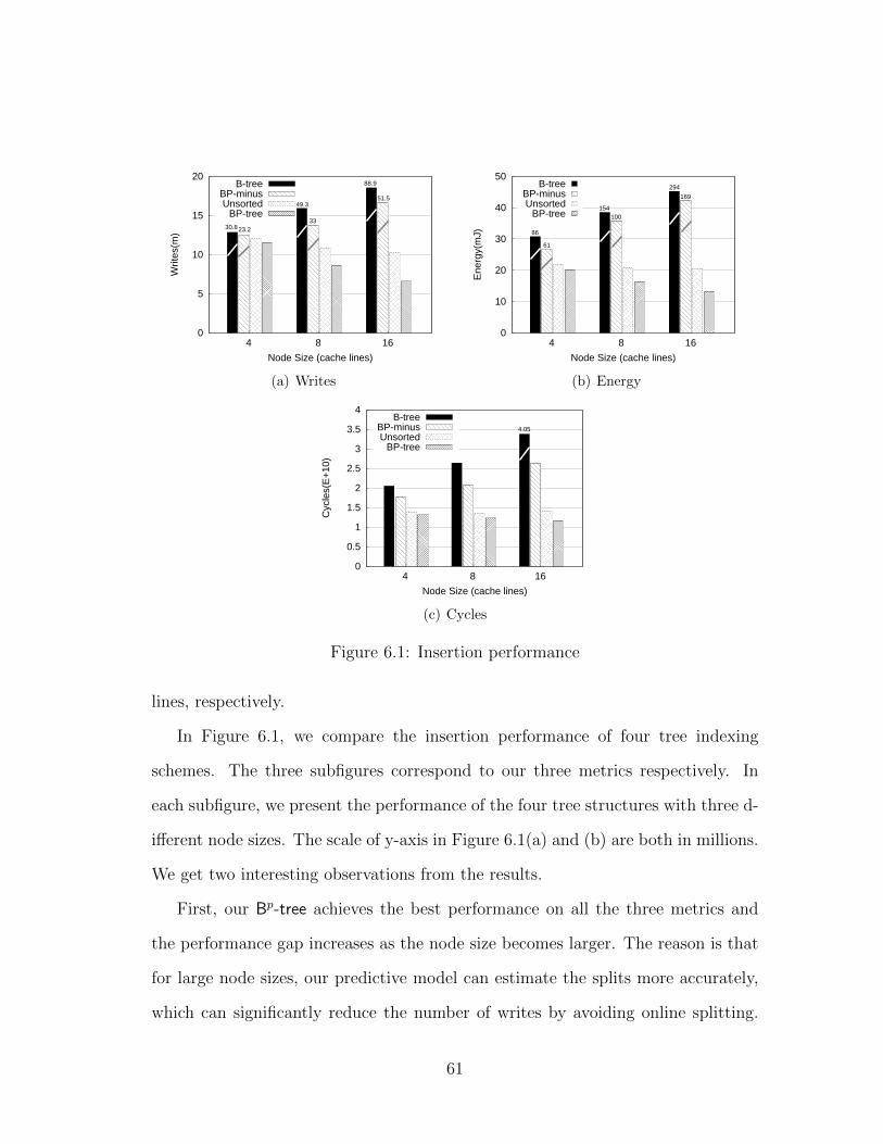
0

5

10

15

20

4 8 16

Writ

es(m

)

Node Size (cache lines)

88.9

51.549.3

3330.823.2

B-treeBP-minusUnsorted BP-tree

(a) Writes

0

10

20

30

40

50

4 8 16

Ene

rgy(

mJ)

Node Size (cache lines)

294

169

154100

86

61

B-treeBP-minusUnsorted BP-tree

(b) Energy

0

0.5

1

1.5

2

2.5

3

3.5

4

4 8 16

Cyc

les(

E+

10)

Node Size (cache lines)

4.05

B-treeBP-minusUnsorted BP-tree

(c) Cycles

Figure 6.1: Insertion performance

lines, respectively.

In Figure 6.1, we compare the insertion performance of four tree indexing

schemes. The three subfigures correspond to our three metrics respectively. In

each subfigure, we present the performance of the four tree structures with three d-

ifferent node sizes. The scale of y-axis in Figure 6.1(a) and (b) are both in millions.

We get two interesting observations from the results.

First, our Bp-tree achieves the best performance on all the three metrics and

the performance gap increases as the node size becomes larger. The reason is that

for large node sizes, our predictive model can estimate the splits more accurately,

which can significantly reduce the number of writes by avoiding online splitting.

61

On the other hand, Unsorted outperforms B+-tree and BP-minus. This is because

most writes will appear in leaf nodes and Unsorted can reduce the number of writes

on leaf nodes. Our Bp-tree outperforms the Unsorted scheme, as it splits the nodes

in advance, which can reduce the numbers of future splits. Bp-tree incurs about

5%, 22%, 37% less PCM writes than the Unsorted scheme on the three different

node sizes respectively. For energy consumption, the result is very similar to that

of the writes. For CPU cycles, the gap becomes slightly smaller because Bp-tree

incurs extra CPU costs on the small B+-tree in the DRAM buffer. However, Bp-tree

still performs better than the Unsorted tree by a factor of 18% when the node size

is 16 cache lines.

Second, we compare the performance of the two tree indexes with sorted leaf

nodes, namely BP-minus and B+-tree. BP-minus outperforms B+-tree in all metrics.

BP-minus reduces about 25%, 33%, 42% of numbers of PCM writes compared to

the B+-tree. Similar trend is observed for the energy consumption. This means that

our Bp-tree outperforms the traditional B+-tree even if we do not want to make the

keys on each node unsorted. For CPU cycles, the gap is not that significant because

of the extra cost on the small B+-tree in the DRAM buffer. Despite this, BP-minus

still reduces 14%, 22%, 35% cost of that of B+-tree.

6.2.2 Update

In this section, we evaluate the update performance of Bp-tree. We first insert all

the keys back-to-back as the previous insertion experiment and then we generate

and run 100k update queries randomly. The update query consists of two keys,

oldKey and newKey. We first search the oldKey. If we find it, we delete it and

insert the newKey. Otherwise, we will ignore the insertion request. In Figure 6.2,

62

we compare the average update performance of our Bp-tree and the other three tree

structures. The result is very close to that of the insertion performance.

Our Bp-tree still achieves the best performance on all the three measures. The

main reason is that our Bp-tree can predict future insertions and can pre-allocate

space to reduce the number of writes. Compared to Unsorted, our Bp-tree reduces

24% of the writes, 26% of the energy and 19% of the CPU cycles, when the node

size is 16 cache lines. If the node size is small, the gap decreases but our Bp-tree

still outperforms Unsorted.

Compared to the traditional B+-tree, the performance of BP-minus is better.

It reduces 14% of the writes, 22% of the energy and 7% of the CPU cycles and the

gap increases as the node size becomes larger. It shows the similar trends for all of

the three measures.

6.2.3 Search

The philosophy of Bp-tree is two-fold: 1) Bp-tree is designed to reduce the number

of writes on PCM, and 2) Bp-tree should be efficient for query processing as well.

In this section, we evaluate the search performance of Bp-tree. The experiments

include point queries and range queries. We experiment on both the uniform and

skewed datasets. We first insert all keys into the index. Then for both point query

and range query, we randomly generate 50k queries and calculate the CPU cycles

during the processing.

In Figure 6.3, we compare the search performance of the four tree indexes. The

left subfigure is for point query and the right one is for range query. The y-axis

represents the total CPU cycles to run these search queries. For point query, the

performance of Bp-tree is better than Unsorted. This is because when we process

63

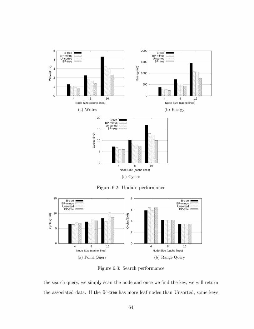
0

1

2

3

4

5

4 8 16

Writ

es(E

+7)

Node Size (cache lines)

B-treeBP-minusUnsorted

BP-tree

(a) Writes

0

500

1000

1500

2000

4 8 16

Ene

rgy(

mJ)

Node Size (cache lines)

B-treeBP-minusUnsorted

BP-tree

(b) Energy

0

5

10

15

20

4 8 16

Cyc

les(

E+

9)

Node Size (cache lines)

B-treeBP-minusUnsorted

BP-tree

(c) Cycles

Figure 6.2: Update performance

0

5

10

15

4 8 16

Cyc

les(

E+

6)

Node Size (cache lines)

B-treeBP-minusUnsorted

BP-tree

(a) Point Query

0

2

4

6

8

4 8 16

Cyc

les(

E+

9)

Node Size (cache lines)

B-treeBP-minusUnsorted

BP-tree

(b) Range Query

Figure 6.3: Search performance

the search query, we simply scan the node and once we find the key, we will return

the associated data. If the Bp-tree has more leaf nodes than Unsorted, some keys

64

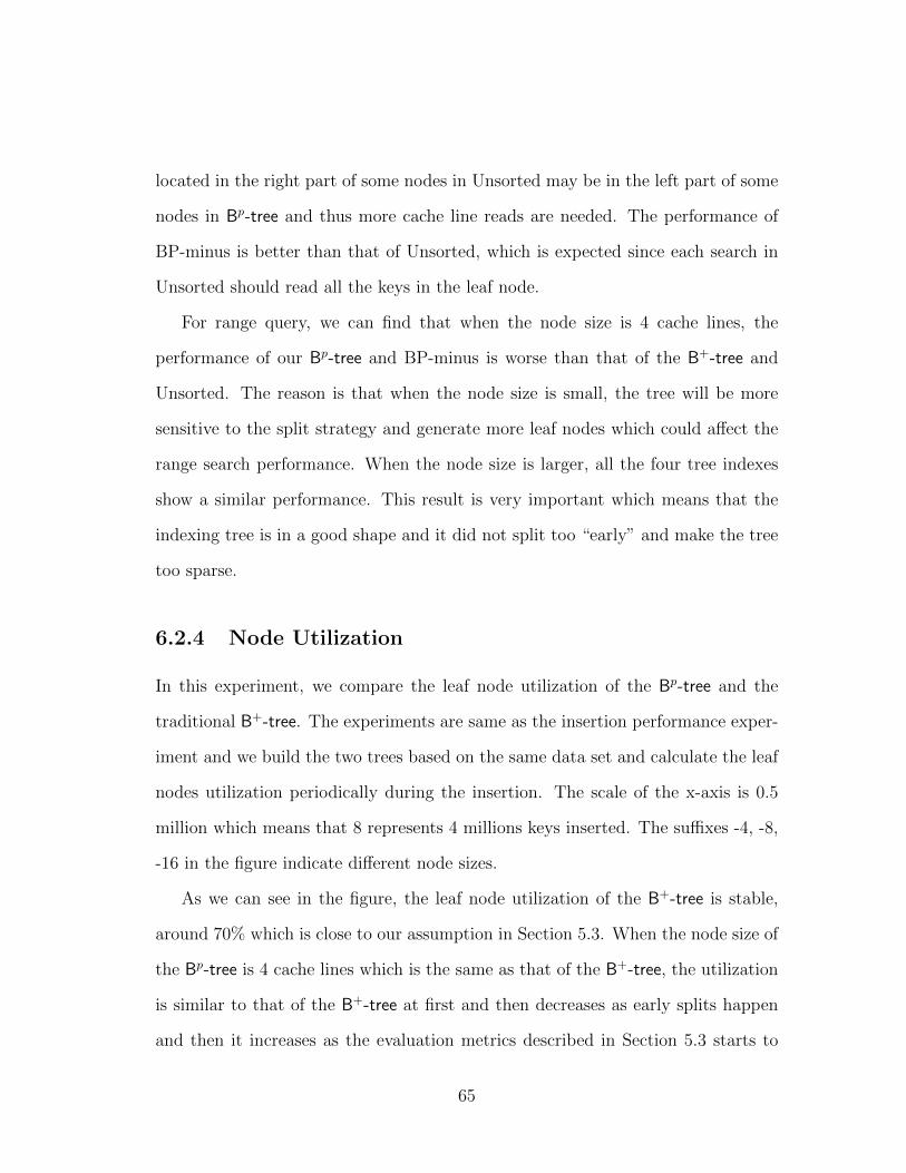
located in the right part of some nodes in Unsorted may be in the left part of some

nodes in Bp-tree and thus more cache line reads are needed. The performance of

BP-minus is better than that of Unsorted, which is expected since each search in

Unsorted should read all the keys in the leaf node.

For range query, we can find that when the node size is 4 cache lines, the

performance of our Bp-tree and BP-minus is worse than that of the B+-tree and

Unsorted. The reason is that when the node size is small, the tree will be more

sensitive to the split strategy and generate more leaf nodes which could affect the

range search performance. When the node size is larger, all the four tree indexes

show a similar performance. This result is very important which means that the

indexing tree is in a good shape and it did not split too “early” and make the tree

too sparse.

6.2.4 Node Utilization

In this experiment, we compare the leaf node utilization of the Bp-tree and the

traditional B+-tree. The experiments are same as the insertion performance exper-

iment and we build the two trees based on the same data set and calculate the leaf

nodes utilization periodically during the insertion. The scale of the x-axis is 0.5

million which means that 8 represents 4 millions keys inserted. The suffixes -4, -8,

-16 in the figure indicate different node sizes.

As we can see in the figure, the leaf node utilization of the B+-tree is stable,

around 70% which is close to our assumption in Section 5.3. When the node size of

the Bp-tree is 4 cache lines which is the same as that of the B+-tree, the utilization

is similar to that of the B+-tree at first and then decreases as early splits happen

and then it increases as the evaluation metrics described in Section 5.3 starts to

65

0.1

0.2

0.3

0.4

0.5

0.6

0.7

0.8

1 2 3 4 5 6 7 8

Leaf

Nod

es U

tiliz

atio

n

Number of Insertions

B-tree-4BP-tree-4BP-tree-8

BP-tree-16

Figure 6.4: Leaf nodes utilization

work. When the node size is 8 cache lines, the utilization is smaller than that of

the B+-tree at first because of the enlargement of the node size and then it starts

to increase. The result for the node size of 16 cache lines is similar. The stable

utilization of all the three different Bp-tree indexes are all slightly smaller than that

of the traditional B+-tree, but according to the previous range search experiment,

the influence of the utilization gap on the range search performance is not obvious

and it is affordable.

6.2.5 Sensitivity to Data Distribution Changes

In this section, we evaluate the sensitivity of our predictive model to data distribu-

tion changes in order to show that our Bp-tree is stable with the dataset of different

data distributions. We change the dataset as follows. The size of the dataset is 5

millions and the dataset follows a skewed (Zipf) distribution. However, we gradual-

ly change the Zipf factors and add a random offset every one million keys generated,

resulting in a change of the data distribution. We did the insertion, update, search

experiments as in previous sections. In Figure 6.5, we show comparisons of the

66

CPU cycles of all the four tree indexes with respect to different operations.

From the figure, we can observe that the relative performance of insertion,

update and point search is very similar to that of the previous experiments. For

the leaf node utilization, when the node size is 4 cache lines, the trend of the first

half is similar to that of the previous result, but the utilization decreases slightly as

the second half starts and increases again at last. The reason of the decrease is that

changes of data distribution caused a wrong prediction from the predictive model

and further caused some improper splits. After that the predictive model adjusts

its prediction via the evaluation metrics and makes the structure normal again

which means that our evaluating scheme works fine and it can help the predictive

model to modify the splitting strategy.

We can also observe from Figure 6.5(e) that the stable utilization value is a

bit smaller than that of the previous experiments, which may have also caused the

range search performance to degrade slightly as shown in Figure 6.5(d). To sum-

marize, the major performance of the Bp-tree verified in the previous experiments

still holds when the data distribution changes which shows Bp-tree to be stable.

6.3 Summary

In this chapter, we did an extensive experiments evaluation of our Bp-tree. We build

our experimental platform to simulate the PCM environment and compare it with

some of the other write-optimized indexing technique and the traditional normal

B+-tree. We did the experiments based on both the uniform dataset and skewed

dataset. We observed that for both data distribution, our Bp-tree can work well.

The experimental results show that the Bp-tree significantly reduces the number of

67

0

2

4

6

4 8 16

Cyc

les(

E+

10)

Node Size (cache lines)

B-treeBP-minusUnsorted

BP-tree

(a) Insertion

0

5

10

15

20

4 8 16

Cyc

les(

E+

9)

Node Size (cache lines)

B-treeBP-minusUnsorted

BP-tree

(b) Update

0

5

10

15

4 8 16

Cyc

les(

E+

6)

Node Size (cache lines)

B-treeBP-minusUnsorted

BP-tree

(c) Point Search

0

10

20

30

4 8 16

Cyc

les(

E+

8)

Node Size (cache lines)

B-treeBP-minusUnsorted

BP-tree

(d) Range Search

0.1

0.2

0.3

0.4

0.5

0.6

0.7

0.8

1 2 3 4 5 6 7 8

Leaf

Nod

es U

tiliz

atio

n

Number of Insertions

B-tree-4BP-tree-4BP-tree-8

BP-tree-16

(e) Leaf Node Utilization

Figure 6.5: Sensitivity to Data Distribution Changes

writes for both the insertions and updates while having a good search performance

at the same time, therefore making it write and energy efficient and suitable for a

PCM-like hardware environment. The sensitivity experiments show that Bp-tree is

68

a stable indexing technique and it works fine for different datasets.

69

Chapter 7

Conclusion

In this chapter, we are going to conclude our work of this thesis and present a

direction for the future work.

7.1 Conclusion

Phase change memory (PCM) is an emerging memory technology with many attrac-

tive features. In the near future, PCM is expected to become a common component

in the memory hierarchy of the computer systems. On one hand, PCM could turn

out to be a low-cost, more reliable, faster and better alternative to flash memory.

On the other hand, PCM is also a very promising alternative to the traditional

DRAM to become the major component of the main memory system.

However, PCM is still in its early stage and we still face some challenges to

design algorithms for PCM-based memory systems including the high read and

write latency compared to DRAM, the limited lifetime of the chip and the high

energy consumption etc. If we want to make best use of PCM in the existing

systems, we need to overcome these challenges.

70

In this thesis, we proposed to study the algorithms redesigning for database sys-

tems on phase change memory, particularly for indexing technique but in the future

we can reconsider the whole technology stack of a traditional database systems. In

our work, we proposed the Bp-tree indexing structure to best take advantage of the

good features of PCM.

The main design objective of our Bp-tree indexing is to reduce the number of

writes and energy consumption while keeping the tree construction and search effi-

cient. We developed a predictive model to predict the near future data distribution

based on the current data and then pre-allocate space for them in the PCM memory

to reduce the movements caused by node splits and merges. We present the details

of the model and show some metrics to evaluate the performance of the model

during the construction process. If the metrics indicate that the prediction model

is not running in a normal manner, we will adjust the model or rebuild the index in

the worst case. The experiments on PostgreSQL database system showed that our

Bp-tree indexing scheme achieves a better performance than the traditional B+-tree

and outperforms the state-of-the-art solution proposed in [6]. Additionally, our

Bp-tree can be easily implemented in existing commercial database systems based

on the existing B+-tree structures.

7.2 Future Work

Database system is a very complex system and it consists of many complex subsystems[28,

9]. Currently we only considered the indexing technique but there are many others

we can work on for example the query processing algorithms.

In the future, we can continue to work on algorithms redesigning for PCM-based

71

database systems. We can gradually move on the the query processing algorithms

and buffer management. Since query processing is an important component of the

database system, which will influence the overall performance of the whole system

greatly, it needs to be redesigned carefully.

In [6], Chen, Gibbons and Nath have already done some work on hash joins.

First they show the simple hash join, there are two phases, the build phase and

the probe phase. In the build phase, the algorithm scans the smaller build relation

and build a hash table for this relation. Then in the probe phase, the algorithm

scans the larger probe relation. For each probe tuple, it computes the hash code

and compare with the hash table to output the join result. The main disadvantage

of the simple hash join is that whenever the size of the recode is large or not, it will

lead to many cache misses, which can lead to a low performance. Then to solve

the cache miss problem, the cache partitioning algorithm is introduced. The major

difference is that in the build phase, instead of hashing the whole relation, the

algorithm partitioned the two input relations using the same hash function so that

every pair of the partitions can fit into the CPU cache. Then in the join phase, for

each pair of the partition, the simple hash join algorithm can be used. The cache

partitioning algorithm can solve the cache miss problem of the simple hash join.

But it introduces a large number of writes which is not suitable for PCM-based

database systems. Thus in this paper, the authors propose the virtual partitioning

hash join, which is a variant of the cache partitioning method. The basic idea is

that instead of physically copying input records into partitions, we perform the

partitioning virtually. For each partition in build phase, we remember the record

IDs and then in the join phase, we can use the record ID lists to join the records

of a pair of partitions in place, thus avoiding the large number of writes in cache

72

partitioning.

In our research, since we want to reduce the writes, we need to reconsider and

redesign the operators if necessary, including scan, sort, join etc. Since PCM does

not have the “erase-before-write” shortage, we do not need to focus on the erase

and block writes. Since PCM supports fast random reads, we can work on the

page layouts like the algorithms design for SSD to reduce the read latency. For

refinement of operators, some of the existing techniques can be used like the “first

index and late materialization” strategy which can reduce much writes.

Much work can be done for the query processing optimization for PCM-based

database systems. In this thesis, we just show a direction and we can continue to

work on this topic in the future.

73

Bibliography

[1] D. Agrawal, D. Ganesan, R. Sitaraman, Y. Diao, and S. Singh. Lazy-adaptive

tree: An optimized index structure for flash devices. PVLDB, 2(1):361–372,

2009.

[2] Anastassia Ailamaki, David J. DeWitt, Mark D. Hill, and Marios Skounakis.

Weaving relations for cache performance. In Proceedings of the 27th Interna-

tional Conference on Very Large Data Bases, VLDB ’01, pages 169–180, San

Francisco, CA, USA, 2001. Morgan Kaufmann Publishers Inc.

[3] Lars Arge. The buffer tree: A new technique for optimal i/o-algorithms.

Algorithms and Data Structures, pages 334–345, 1995.

[4] D. Bausch, I. Petrov, and A. Buchmann. On the performance of database

query processing algorithms on flash solid state disks. In Database and Expert

Systems Applications (DEXA), 2011 22nd International Workshop on, pages

139–144. IEEE, 2011.

[5] F. Bedeschi, R. Fackenthal, C. Resta, EM Donze, M. Jagasivamani, E. Buda,

F. Pellizzer, D. Chow, A. Cabrini, G.M.A. Calvi, et al. A multi-level-cell

bipolar-selected phase-change memory. In Solid-State Circuits Conference,

74

2008. ISSCC 2008. Digest of Technical Papers. IEEE International, pages

428–625. IEEE, 2008.

[6] S. Chen, P.B. Gibbons, and S. Nath. Rethinking Database Algorithms for

Phase Change Memory. CIDR, 2011.

[7] Douglas Comer. The ubiquitous b-tree. ACM Comput. Surv., 11(2):121–137,

1979.

[8] Jeremy Condit, Edmund B. Nightingale, Christopher Frost, Engin Ipek, Ben-

jamin Lee, Doug Burger, and Derrick Coetzee. Better i/o through byte-

addressable, persistent memory. In Proceedings of the ACM SIGOPS 22nd

symposium on Operating systems principles, SOSP ’09, pages 133–146, New

York, NY, USA, 2009. ACM.

[9] CJ Date. An introduction to database systems , vol. iiaddison-wesley. Reading,

MA, 1983.

[10] Goetz Graefe. Write-optimized b-trees. In Proceedings of the Thirtieth in-

ternational conference on Very large data bases-Volume 30, pages 672–683,

2004.

[11] Peter J. Haas and Joseph M. Hellerstein. Ripple joins for online aggregation.

In Proceedings of the 1999 ACM SIGMOD international conference on Man-

agement of data, SIGMOD ’99, pages 287–298, New York, NY, USA, 1999.

ACM.

[12] J.M. Hellerstein, M.J. Franklin, S. Chandrasekaran, A. Deshpande, K. Hil-

drum, S. Madden, V. Raman, and M.A. Shah. Adaptive query processing:

Technology in evolution. IEEE Data Engineering Bulletin, 23(2):7–18, 2000.

75

[13] Navin Kabra and David J. DeWitt. Efficient mid-query re-optimization of

sub-optimal query execution plans. 27(2):106–117, June 1998.

[14] Benjamin C. Lee, Engin Ipek, Onur Mutlu, and Doug Burger. Architecting

phase change memory as a scalable dram alternative. In Proceedings of the

36th annual international symposium on Computer architecture, ISCA ’09,

pages 2–13. ACM, 2009.

[15] Yinan Li, Bingsheng He, Robin Jun Yang, Qiong Luo, and Ke Yi. Tree in-

dexing on solid state drives. Proceedings of the VLDB Endowment, 3(1):1195–

1206, 2010.

[16] Soumyadeb Mitra, Windsor W. Hsu, and Marianne Winslett. Trustworthy

keyword search for regulatory-compliant record retention. In Proceedings of

the International Conference on Very Large Data Bases, pages 1001–1012,

2006.

[17] G. Muller, N. Nagel, C.U. Pinnow, and T. Rohr. Emerging non-volatile mem-

ory technologies. In Proceedings of the 29th European Solid-State Circuits

Conference, ESSCIRC ’03, pages 37–44. IEEE, 2003.

[18] K.G. Murty. Supply chain management in the computer industry. Technical

report, Working Paper, University of Michigan Department of Industrial and

Operations Engineering, 2000.

[19] K.G. Murty. Histogram, an ancient tool and the art of forecasting. Technical

report, Citeseer, 2002.

76

[20] Suman Nath and Aman Kansal. Flashdb: dynamic self-tuning database for

nand flash. In Proceedings of the 6th international conference on Information

processing in sensor networks, IPSN ’07, pages 410–419. ACM, 2007.

[21] Patrick O’Neil, Edward Cheng, Dieter Gawlick, and Elizabeth O’Neil. The

log-structured merge-tree (lsm-tree). Acta Informatica, 33(4):351–385, 1996.

[22] P.E. O’Neil. Thesb-tree an index-sequential structure for high-performance

sequential access. Acta Informatica, 29(3):241–265, 1992.

[23] Hwee Hwa Pang, Michael J. Carey, and Miron Livny. Partially preemptible

hash joins. In Proceedings of the 1993 ACM SIGMOD international conference

on Management of data, SIGMOD ’93, pages 59–68, New York, NY, USA,

1993. ACM.

[24] Hweehwa Pang, Michael J. Carey, and Miron Livny. Memory-adaptive external

sorting. In 19th International Conference on Very Large Data Bases, pages

618–629. Morgan Kaufmann, 1993.

[25] Jian Pei, Man Ki Mag Lau, and Philip S. Yu. Ts-trees: A non-alterable search

tree index for trustworthy databases on write-once-read-many (worm) storage.

In AINA, pages 54–61, 2007.

[26] Moinuddin K. Qureshi, John Karidis, Michele Franceschini, Vijayalakshmi S-

rinivasan, Luis Lastras, and Bulent Abali. Enhancing lifetime and security

of pcm-based main memory with start-gap wear leveling. In Proceedings of

the 42nd Annual IEEE/ACM International Symposium on Microarchitecture,

MICRO ’42, pages 14–23. ACM, 2009.

77

[27] Moinuddin K. Qureshi, Vijayalakshmi Srinivasan, and Jude A. Rivers. Scalable

high performance main memory system using phase-change memory technol-

ogy. In Proceedings of the 36th annual international symposium on Computer

architecture, ISCA ’09, pages 24–33. ACM, 2009.

[28] R. Ramakrishnan, J. Gehrke, and J. Gehrke. Database management systems.

McGraw-Hill, 2003.

[29] Vijayshankar Raman, Bhaskaran Raman, and Joseph M. Hellerstein. Online

dynamic reordering. The VLDB Journal, 9(3):247–260, December 2000.

[30] Luiz E. Ramos, Eugene Gorbatov, and Ricardo Bianchini. Page placement

in hybrid memory systems. In Proceedings of the international conference on

Supercomputing, ICS ’11, pages 85–95. ACM, 2011.

[31] S. Raoux, GW Burr, MJ Breitwisch, CT Rettner, Y.C. Chen, RM Shelby,

M. Salinga, D. Krebs, S.H. Chen, H.L. Lung, et al. Phase-change random

access memory: A scalable technology. IBM Journal of Research and Devel-

opment, 52(4.5):465–479, 2008.

[32] Mendel Rosenblum and John K. Ousterhout. The design and implementation

of a log-structured file system. In Proceedings of the thirteenth ACM sympo-

sium on Operating systems principles, SOSP ’91, pages 1–15. ACM, 1991.

[33] Stuart Schechter, Gabriel H. Loh, Karin Straus, and Doug Burger. Use ecp,

not ecc, for hard failures in resistive memories. In Proceedings of the 37th

annual international symposium on Computer architecture, ISCA ’10, pages

141–152. ACM, 2010.

78

[34] Nak Hee Seong, Dong Hyuk Woo, and Hsien-Hsin S. Lee. Security refresh:

Prevent malicious wear-out and increase durability for phase-change memory

with dynamically randomized address mapping. In Proceedings of the 37th

annual international symposium on Computer architecture, ISCA ’10, pages

383–394. ACM, 2010.

[35] M.A. Shah, S. Harizopoulos, J.L. Wiener, and G. Graefe. Fast scans and joins

using flash drives. In Proceedings of the 4th international workshop on Data

management on new hardware, pages 17–24. ACM, 2008.

[36] D. Tsirogiannis, S. Harizopoulos, M.A. Shah, J.L. Wiener, and G. Graefe.

Query processing techniques for solid state drives. In Proceedings of the

35th SIGMOD international conference on Management of data, pages 59–

72. ACM, 2009.

[37] T. Urhan and M.J. Franklin. Xjoin: A reactively-scheduled pipelined join

operatory. Bulletin of the Technical Committee on, page 27, 2000.

[38] H. Wong, S. Raoux, S.B. Kim, J. Liang, J.P. Reifenberg, B. Rajendran,

M. Asheghi, K.E. Goodson, et al. Phase change memory. Proceedings of

the IEEE, 98(12):2201–2227, 2010.

[39] Chin-Hsien Wu, Tei-Wei Kuo, and Li Ping Chang. An efficient b-tree lay-

er implementation for flash-memory storage systems. ACM Transactions on

Embedded Computing Systems (TECS), 6(3):19–es, 2007.

[40] Weiye Zhang and Per-AAke Larson. Dynamic memory adjustment for external

mergesort. In Proceedings of the 23rd International Conference on Very Large

79

Data Bases, VLDB ’97, pages 376–385, San Francisco, CA, USA, 1997. Morgan

Kaufmann Publishers Inc.

[41] Ping Zhou, Bo Zhao, Jun Yang, and Youtao Zhang. A durable and energy

efficient main memory using phase change memory technology. In Proceedings

of the 36th annual international symposium on Computer architecture, ISCA

’09, pages 14–23. ACM, 2009.

80