red blood cell distribution in simpliﬁed capillary...

Phil. Trans. R. Soc. A (2010) 368, 2897–2918doi:10.1098/rsta.2010.0045

Red blood cell distribution in simplifiedcapillary networks

BY DOMINIK OBRIST1,*, BRUNO WEBER2, ALFRED BUCK3

AND PATRICK JENNY1

1Institute of Fluid Dynamics, ETH Zurich, Zurich, Switzerland2Institute of Pharmacology and Toxicology, University of Zurich,

Zurich, Switzerland3Division of Nuclear Medicine, University Hospital Zurich, Zurich, Switzerland

A detailed model of red blood cell (RBC) transport in a capillary network is anindispensable element of a comprehensive model for the supply of the human organismwith oxygen and nutrients. In this paper, we introduce a two-phase model for theperfusion of a capillary network. This model accounts for the special role of RBCs,which have a strong influence on network dynamics. Analytical results and numericalsimulations with a discrete model and a generic network topology indicate that thereexists a local self-regulation mechanism for the flow rates and a global de-mixing processthat leads to an inhomogeneous haematocrit distribution. Based on the results from thediscrete model, we formulate an efficient algorithm suitable for computing the pressureand flow field as well as a continuous haematocrit distribution in large capillary networksat steady state.

Keywords: microcirculation; capillary network; red blood cell transport; bifurcation law

1. Introduction

Recent numerical studies of cerebral blood flow (Boas et al. 2008; Reichold et al.2009) modelled the perfusion of large vascular trees as complex three-dimensionalpipe networks with a viscous flow. The flow and pressure field in such networkscan be simulated on the basis of Kirchhoff’s laws for electrical networks. Thisinvolves very large systems of linear equations. In order to reduce the total sizeof these systems, the lowest levels of the vascular tree, i.e. the capillaries, can betreated as a spatial continuum with a given permeability that is based on the localmorphology of the capillary network. We will show that this approach falls shortof describing the perfusion of a capillary network because it neglects the role ofthe red blood cells (RBCs). In capillary networks, blood must not be modelledas a single viscous phase. Rather, the transport of RBCs and the plasma phaseare to be treated separately. This leads to perfusion characteristics that differstrongly from single-phase models.

*Author for correspondence ([email protected]).

One contribution of 13 to a Theme Issue ‘The virtual physiological human: computer simulationfor integrative biomedicine II’.

This journal is © 2010 The Royal Society2897

on July 14, 2018http://rsta.royalsocietypublishing.org/Downloaded from

mailto:[email protected]

http://rsta.royalsocietypublishing.org/

2898 D. Obrist et al.

The role of RBCs in the dynamics of the microcirculation has been recognized,studied and discussed in a series of papers in the 1980s and 1990s (e.g.Schmid-Schönbein et al. 1980; Papenfuss & Gross 1981; Klitzman & Johnson1982; Dawant et al. 1986a,b; Pries et al. 1986, 1989, 1990, 1992; Secomb et al.1986). It was shown that the dynamics in a capillary network is much more thanjust the ‘sum’ of viscous flows through narrow pipes. The local concentrationof RBCs has a strong impact on the local flow resistance, which influencesthe flow and pressure fields in the whole network. Schmid-Schönbein et al.(1980) illustrated local self-regulation mechanisms that tend to balance theflow rates in capillaries diverging from the same parent vessel. Unfortunately,it appears that many of today’s researchers are not aware of these results.Therefore, this paper revisits the basic discrete model for RBC transportin capillary networks (as outlined by Pries et al. (1990)). Based on thisapproach, we will formulate a new continuous algorithm to solve for thepressure, flow and haematocrit distribution in a capillary network. This algorithmis efficient and well suited for today’s applications that often use largemorphological datasets of vascular networks (Reichold et al. 2009; Tsai et al.2009). We will show for some idealized configurations that the equations forthe pressure field can be decoupled from the equations for the flow field andhaematocrit distribution. Furthermore, we will present some principal resultsfor capillary networks and discuss their consequences for the perfusion of thesenetworks. In particular, we will stress the differences between the transportof substances in capillary networks with and without RBCs (two phase versussingle phase).

We will introduce the theory in a general framework since the presented resultsapply to the wider field of particulate flows in pipe networks (or even porousmedia) with the only conditions that the Reynolds number is sufficiently smalland that the particle size is comparable to the pipe diameter. In order to reveal theprincipal phenomena in a clear way, we will idealize and simplify the configurationas far as possible. A more detailed description of the local physical phenomenawould not change the global dynamics in a fundamental way, but only take offsome of the rough edges of the results discussed here.

2. Governing equations for red blood cell transport in a capillary network

We model capillary networks as sets of nodes that are connected by rigid pipeswith circular cross sections. A pipe connecting node i with node j has a length Lijand a constant diameter Dij . We require that the diameter of the pipes is small,i.e. Lij � Dij .

The local Reynolds number in a capillary with diameter D and bulk velocityu is defined as Re = Dr|u|/m = 4|q|/(pDm), where r is the fluid density, m thedynamic viscosity of the fluid (i.e. the plasma) and q the mass flow rate. Incapillary networks, this Reynolds number is smaller than unity.

The network transports particles (RBCs) with the same density as thecarrier fluid. The RBCs are deformable and incompressible such that thevolume is preserved even when their shape changes. Their size is of the orderof the capillary diameter such that there is only a narrow lubrication gapbetween an RBC and the vessel wall. They form a single file as they are

Phil. Trans. R. Soc. A (2010)



RBC transport in capillary networks 2899

advected through a capillary. Further, we assume that the RBCs are flexibleenough to pass through each capillary in the network and there is no blockageof capillaries.

Because of the small Reynolds number, the plasma velocity field u and thepressure p are governed by the Stokes equation

mV2u = Vp (2.1)

and the continuity equationV · u = 0. (2.2)

These equations assume implicitly that the flow field is stationary or atleast changing so slowly that the term rvu/vt of the unsteady Stokesequation is negligible with respect to the other terms in equation (2.1). Adimensional analysis of the situation in the microcirculation confirms that this isthe case.

(a) Flow without red blood cells

For a one-dimensional flow through a pipe, it follows directly from equation(2.1) that the mass flow rate qij is proportional to the pressure drop between thetwo adjacent nodes, i.e.

qij = pi − pj

Rij, (2.3)

where pi and pj are the pressure values at the nodes i and j , respectively. Thenominal resistance Rij is given by

Rij = rijLij , (2.4)

where rij is the specific resistance of the capillary. According to Poiseuille’s law(Sutera & Skalak 1993), it is given by

rij = 128m

pD4ijr

. (2.5)

The linear relationship between pressure drop and mass flux drastically simplifiesthe flow calculations. In analogy to Kirchhoff’s first rule for electrical networks,we formulate an equation for the mass balance at each node i,∑

j

qij =∑

j

pi − pj

Rij= qi , (2.6)

where qi is a source term describing a flux into or out of the network at nodei (except at the in- and outflow of the network, we set qi typically to zero).This results in a system of linear equations. To close the system, we have tofix one node pressure by a Dirichlet boundary condition (e.g. by setting thepressure at the outflow to zero). The linear system of equations (2.6) is thediscrete equivalent to Darcy’s law coupled with mass balance. Its solution yieldsall node pressure values pi , and the flow rates qij can then be computed fromequation (2.3).





?

?L ij

Lij

Lij

qij uij

Rijqij + 2Dij

Dij

p

Dij

node i node j

Figure 1. Pressure distribution in a capillary of diameter Dij and length Lij connecting the nodes iand j with a mass flow rate qij and two RBCs of length Lij with a velocity uij . The sketch indicatesalso the typical velocity profiles between two RBCs (Poiseuille) and around an RBC (Couette).

(b) Flow with red blood cells

The situation becomes more complex with the presence of RBCs. Because of thesmall Reynolds numbers and the quasi-stationary flow field, we may neglect theRBC inertia. This means also that the RBC velocities adjust ‘immediately’ tobalance the pressure and the viscous forces.

In general, the flow resistance of a capillary will increase if RBCs are present.This increase is related to the altered flow field in the vicinity of an RBC (figure 1).Instead of a Poiseuille flow profile, we find a narrow shear flow (similar to Couetteflow) in the narrow gap between an RBC and the vessel wall. This shear flow leadsto an increased wall shear stress and, thus, to a higher resistance. The additionalpressure drop Dij owing to an RBC can be written as

Dij = qij Lij [r ij − rij ], (2.7)

where Lij is the effective length of the section in which the velocity profile isinfluenced by the RBC, and r ij is the specific resistance within that section.

The additional pressure drop is illustrated in figure 1 for a capillary with twoRBCs. The total pressure drop in the pipe i–j with Nij RBCs is then

pi − pj = qijRij + Nij Dij = qijReij , (2.8)

where we have introduced the effective resistance

Reij = Rij

(1 + Hijbij

), (2.9)

with the tube haematocrit

Hij = Nij Lij

Lij(2.10)

and

bij = r ij

rij− 1. (2.11)





The variable bij is typically of order 1 and is known as the apparent intrinsicviscosity (Secomb et al. 1986). Several numerical results illustrate the dependenceof bij on various flow parameters (Pozrikidis 2003, 2005a,b) and on the endothelialsurface layer (ESL) (Secomb et al. 2003). In the present work, we simply assumethat bij is a constant property of a capillary and of order 1. This idealizationis legitimate because we will see in §3b that one of the central mechanismsin capillary networks does not depend on the exact form of equation (2.9),but only requires that the effective resistance increases monotonically with thehaematocrit. Similar to equation (2.6), we can use the effective resistance Re

ij toderive a linear system of equations∑

j

pi − pj

Reij

= qi , (2.12)

which yields the node pressure values in a network with RBCs.The velocity of an RBC is given by

uij = uij qij = 4qij qij

prD2ij

, (2.13)

where the coefficient qij ≥ 1 corrects the RBC velocity with respect to the meanvelocity uij . Very tightly fitting RBCs will be advected with the mean fluidvelocity (qij = 1), whereas RBCs at the centreline of very large blood vessels(e.g. arteries) will be advected nearly with the peak fluid velocity (qk

ij → 2).The velocity correction coefficient qij is directly related to the Fåhræus effectin capillaries (Albrecht et al. 1979).

(c) Bifurcation rule

If the RBC locations in the network are given, the pressure and flow field canbe computed from equations (2.9) and (2.12). Equation (2.13) can then be usedto compute the RBC velocities with which the RBCs are advected. As long asthe RBCs remain within their capillary, this propagation is well defined and thepressure and flow field do not change. Once an RBC arrives at a bifurcation, itwill enter a different capillary such that the effective resistance Re

ij changes andthe pressure and flow fields have to be recomputed.

To decide which capillary the RBC will enter, we need a bifurcation rule. Atfirst glance, the RBC dynamics at a bifurcation appears to be a very complexmatter that does not only depend on the local flow field but also on the exactbifurcation geometry and RBC properties. Intuitively, we would assume thatan RBC prefers the capillary that requires the least change in direction. Thisreasoning is motivated by the inertia of the RBC. In our case, however, we havea low-Reynolds-number configuration governed by the Stokes equation (2.1) thatdoes not contain any inertial terms. Therefore, we postulate that the RBCs willfollow the path of the steepest pressure gradient (regardless of their inertia).Further, we assume that the work required to deform an RBC (e.g. to squeeze itinto a capillary with a smaller diameter) is negligible (Secomb & Hsu 1996). Weformalize the bifurcation rule as follows: an RBC at node i will enter the pipe





i–j ∗ with the highest negative pressure gradient

Gij ∗ = maxj

{Gij}, (2.14)

where the local pressure gradient Gij of the pipe i–j is given by

Gij = qij rij . (2.15)

Note that Gij does not depend on the effective resistance Reij , but rather on the

specific resistance rij , because the RBC at the bifurcation only ‘feels’ the localpressure gradient and does not ‘see’ what is behind the bifurcation (cf. figure 1).Therefore, the bifurcation dynamics is not directly influenced by any obstacle,constriction or dilation behind the bifurcation.

Note that this formulation of the bifurcation rule is different from thebifurcation rule used in older studies (e.g. Klitzman & Johnson 1982; Pries et al.1990), where the models for the bifurcation dynamics are based on empiricalresults (e.g. Fung 1973; Pries et al. 1989). Our bifurcation rule is motivated byphysical arguments and follows from a strict analysis of an idealized configuration.It may neglect some of the more subtle effects present at a bifurcation (e.g. RBCdeformation), but has the advantage that it can be used to derive analyticalresults for capillary networks (as will be shown, for instance, in §4a).

In idealized configurations where the local specific resistances rij are equal forall diverging vessels, an RBC will prefer the capillary with the highest flow rate.In this case, our bifurcation rule is consistent with the bifurcation rule used bySchmid-Schönbein et al. (1980). Therefore, it can be considered an idealizationof the experimental findings by Fung (1973) and Pries et al. (1989), and it isconsistent with the more recent numerical results by Barber et al. (2008) if onlynarrow vessels are considered.

3. Discrete model: red blood cell transport in capillary networks

The mass balance at the bifurcations, the effective resistance and the bifurcationrule constitute a complete model for the RBC transport in a capillary network.The basic simulation algorithm reads as follows:

(1) Choose initial RBC positions.(2) Compute effective resistance Re

ij using equation (2.9).(3) Set up a linear system of equations according to equation (2.12).(4) Solve the linear system of equations for node pressure values pi .(5) Compute flow rates qij from equation (2.8).(6) Propagate the RBCs with the RBC velocities (2.13) until the first RBC

reaches a bifurcation.(7) Apply the bifurcation rule (2.14) to assign the RBC to a new capillary.(8) Continue with step 2.

Schmid-Schönbein et al. (1980) was the first to use such an algorithm to simulateblood flow in the microcirculation. Although they studied only a small networkwith 12 vessels, their results revealed a self-regulation mechanism for flow ratesin the vessels diverging from a bifurcation (see discussion below).





We use this algorithm in the following to study the dynamics in a generic squarenetwork. It consists of nodes i = I (i1, i2) with 1 ≤ i1, i2 ≤ n, which are arranged ina square. Each node is connected to its neighbours, i.e. to the nodes I (max(1, i1 −1), i2), I (min(n, i1 + 1), i2), I (i1, max(1, i2 − 1)) and I (i1, min(n, i2 + 1)). Theinflow is at the node I (1, 1) with a constant flow rate q0 > 0 and the outflow with−q0 at the node I (n, n). The pressure at the outflow node I (n, n) is set to zero.

Such a network is the simplest possible configuration for studying basicmechanisms of RBC transport. Although it cannot be found in nature, it is wellsuited for illustrating the dramatic differences between a single- and a two-phasemodel.

For the following numerical experiments, a network with n = 11 is seededrandomly with np = 550 RBCs (uniformly distributed), which corresponds to anaverage haematocrit of 0.4. The network is homogeneous in the sense that allcapillaries have the same physical properties (D = 5 mm, L = 50 mm, L = 8 mm,b = 2.7, q = 1). The number of RBCs is held constant by reinjecting all RBCsthat exit the network through the outflow. The mass flow rate at the inflow isset to q0 = rpD2/4 × 10−3 ms−1. The fluid (i.e. the plasma) is assumed to havedensity r = 1050 kg m−3 and dynamic viscosity m = 1.5 × 10−3 kg ms−1.

(a) Transition towards a steady-state configuration

Figure 2 shows the network with the RBCs at different times. Startingwith the uniformly distributed initial condition (figure 2a), the network goesthrough a transient phase (figure 2b,c), during which the uniform haematocritdistribution becomes increasingly inhomogeneous. Eventually, this de-mixing ofthe RBC and plasma phases reaches a statistically steady state (figure 2d) inthe sense that the ensemble averages of the flow field, the pressure field andthe haematocrit distribution are constant in time. The duration of the transientphase is comparable to the total network turnover time t = 11 s, which is definedas the ratio of the total network volume to the volumetric flow rate q0/r atthe inflow. The particular steady-state configuration is a direct consequence ofthe bifurcation rule and of the effective resistance that depends on the localhaematocrit. For the given network topology, the steady-state configurationexhibits a low haematocrit and a relatively high flow rate in the centre of thenetwork. An ‘RBC highway’ emerges along the main diagonal, while the RBCsin the outer corners accumulate and stagnate.

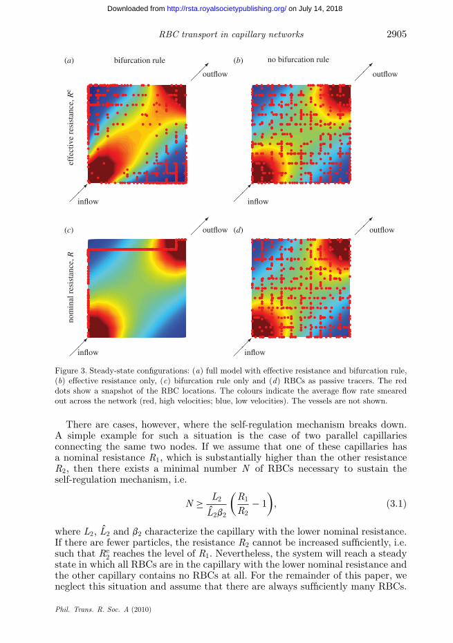
In order to illustrate the relevance of the bifurcation rule and the effectiveresistance, we show in figure 3 four different steady-state solutions. Only figure 3ahas been obtained with the full model. In the three other plots, the effectiveresistance and/or the bifurcation rule have been replaced by the nominalresistance Rij and/or by a random bifurcation (biased by the local flow rate).Only the full model exhibits a low particle concentration and a relatively highflow rate in the centre of the network. If the bifurcation rule is switched off(figure 3b,d), the particles maintain their uniform distribution across the wholenetwork. The flow rates in figure 3c,d are identical because the effective resistanceis replaced by the nominal resistance such that the flow field is independent ofthe particles (single-phase flow). In figure 3c, the RBCs follow the path of thesteepest pressure gradient. In figure 3d, the RBCs act as passive tracers that arecarried along with the fluid without influencing the flow.





outflow

inflow

(a) (b)

(c) (d)

outflow

inflow

outflow

inflow

outflow

inflow

Figure 2. Generic capillary network with 11 × 11 rows and columns of capillaries. The network isseeded randomly with 550 RBCs (black dots). The RBCs at the outflow (b) are reinjected throughthe inflow (d). (a) t/t = 0; (b) t/t = 0.5; (c) t/t = 1.0; (d) t/t = 1.5.

(b) Self-regulation mechanism

The steady-state configuration in a network is the global result of a localphenomenon, i.e. the self-regulation mechanism. Schmid-Schönbein et al. (1980)described this mechanism for a bifurcation with two identical diverging vessels.Here, we discuss the mechanism in the context of our more general bifurcationrule. According to this rule, an RBC arriving at a bifurcation moves intothe capillaries with the highest pressure gradient. This increases the effectiveresistance and thus reduces the flow rate and the pressure gradient. This processcontinues until another capillary has the highest pressure gradient. On average,an equilibrium is attained where all capillaries (with qij > 0) have the samepressure gradient. For capillaries with equal specific resistances rij , this processis tantamount to a self-regulation mechanism that leads to equal flow rates in alldivergent capillaries, as reported by Schmid-Schönbein et al. (1980). Their resultsshow also that the self-regulation mechanism is able to adjust the flow rates veryrapidly, i.e. the time necessary to attain a statistical equilibrium is of the orderof the network turnover time.





bifurcation rule(a) (b)

(c) (d)

no bifurcation ruleef

fect

ive

resi

stan

ce, R

eoutflow

inflow

outflow

inflow

outflow

inflow

outflow

inflow

nom

inal

res

ista

nce,

R

Figure 3. Steady-state configurations: (a) full model with effective resistance and bifurcation rule,(b) effective resistance only, (c) bifurcation rule only and (d) RBCs as passive tracers. The reddots show a snapshot of the RBC locations. The colours indicate the average flow rate smearedout across the network (red, high velocities; blue, low velocities). The vessels are not shown.

There are cases, however, where the self-regulation mechanism breaks down.A simple example for such a situation is the case of two parallel capillariesconnecting the same two nodes. If we assume that one of these capillaries hasa nominal resistance R1, which is substantially higher than the other resistanceR2, then there exists a minimal number N of RBCs necessary to sustain theself-regulation mechanism, i.e.

N ≥ L2

L2b2

(R1

R2− 1

), (3.1)

where L2, L2 and b2 characterize the capillary with the lower nominal resistance.If there are fewer particles, the resistance R2 cannot be increased sufficiently, i.e.such that Re

2 reaches the level of R1. Nevertheless, the system will reach a steadystate in which all RBCs are in the capillary with the lower nominal resistance andthe other capillary contains no RBCs at all. For the remainder of this paper, weneglect this situation and assume that there are always sufficiently many RBCs.





500

2

4

6

8

10

12

14

16

18

20

0 50 0 50 0 50 0 50x (µm)

t (s)

x (µm) x (µm) x (µm) x (µm)

1 2 3 4 5

54321

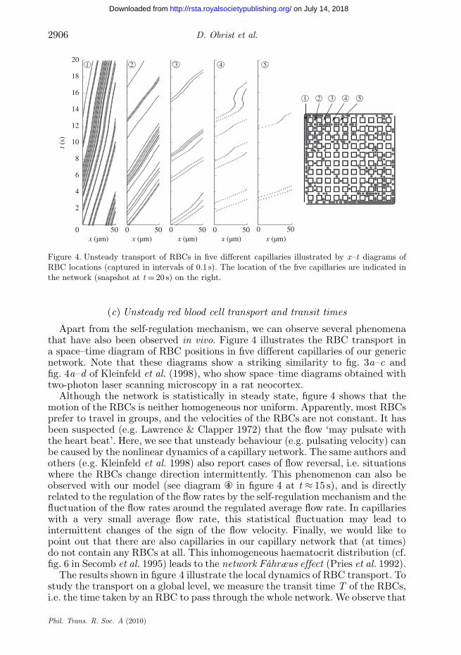
Figure 4. Unsteady transport of RBCs in five different capillaries illustrated by x–t diagrams ofRBC locations (captured in intervals of 0.1 s). The location of the five capillaries are indicated inthe network (snapshot at t = 20 s) on the right.

(c) Unsteady red blood cell transport and transit times

Apart from the self-regulation mechanism, we can observe several phenomenathat have also been observed in vivo. Figure 4 illustrates the RBC transport ina space–time diagram of RBC positions in five different capillaries of our genericnetwork. Note that these diagrams show a striking similarity to fig. 3a–c andfig. 4a–d of Kleinfeld et al. (1998), who show space–time diagrams obtained withtwo-photon laser scanning microscopy in a rat neocortex.

Although the network is statistically in steady state, figure 4 shows that themotion of the RBCs is neither homogeneous nor uniform. Apparently, most RBCsprefer to travel in groups, and the velocities of the RBCs are not constant. It hasbeen suspected (e.g. Lawrence & Clapper 1972) that the flow ‘may pulsate withthe heart beat’. Here, we see that unsteady behaviour (e.g. pulsating velocity) canbe caused by the nonlinear dynamics of a capillary network. The same authors andothers (e.g. Kleinfeld et al. 1998) also report cases of flow reversal, i.e. situationswhere the RBCs change direction intermittently. This phenomenon can also beobserved with our model (see diagram ④ in figure 4 at t ≈ 15 s), and is directlyrelated to the regulation of the flow rates by the self-regulation mechanism and thefluctuation of the flow rates around the regulated average flow rate. In capillarieswith a very small average flow rate, this statistical fluctuation may lead tointermittent changes of the sign of the flow velocity. Finally, we would like topoint out that there are also capillaries in our capillary network that (at times)do not contain any RBCs at all. This inhomogeneous haematocrit distribution (cf.fig. 6 in Secomb et al. 1995) leads to the network Fåhræus effect (Pries et al. 1992).

The results shown in figure 4 illustrate the local dynamics of RBC transport. Tostudy the transport on a global level, we measure the transit time T of the RBCs,i.e. the time taken by an RBC to pass through the whole network. We observe that





2 4 6 8 100

0.05

0.10

0.15

0.20

0.25

T/τ

Figure 5. Normalized histogram (evaluated over 100t) of the RBC transit time T (red) comparedwith the transit time of passive tracers in a network without RBCs (blue).

some RBCs pass rapidly along the main ‘highway’ towards the outlet, while manyRBCs take a slower route via the periphery of the network. This is reflected in thehistogram of the transit times (figure 5). For comparison, we also show the transittimes of passive tracer particles that are equivalent to a single-phase model. Whileboth histograms peak at around T = t, we observe that the transit time variesless for passive tracer particles than for RBCs (long tail in the histogram). At thesame time, the fastest RBCs traverse the network slightly faster than the fastestpassive tracers. It is also worthwhile to note that the two peaks around T/t = 5and 6.5 appear to be genuine in the sense that the statistics have converged. Thepreference for these two transit times is probably related to the specific networktopology, but is not fully understood at the moment.

4. Continuous model: dynamics in steady state

We have seen in §3b that the self-regulation mechanism regulates the pressuregradients in the diverging blood vessels of a bifurcation. This local mechanismleads to steady-state configurations of the whole network.

To make further progress in investigating the dynamics of steady-stateconfigurations, we assume that Lij � Lij and r ij � rij . It is then a valididealization to consider the haematocrit Hij ≥ 0 to be a continuous real number.In contrast to the previous section, where we tracked discrete RBCs in a transientprocess, we will now study the dynamics of a stationary system with continuousvariables. We use the haematocrit to formulate an equation for the conservationof RBCs within the network, i.e. we require that the sum of all RBC mass flowrates at a bifurcation is zero. This is similar to the application of Kirchhoff’s firstrule in equation (2.6), except that we are now directly involving the haematocritin our equations. Further, we formulate a reordering approach for determining theflow rates. This will allow us to determine the steady-state solution in an iterativeprocess. A similar scheme was used by Papenfuss & Gross (1981) and Dawantet al. (1986a,b) to study the haematocrit distribution in microvascular networks.





Here, we will formulate an algorithm that makes use of our specific formulationof the bifurcation rule. This algorithm is able to solve the governing equations inan efficient manner such that it is well suited for studying very large networks.We will use this algorithm to illustrate some basic phenomena. Furthermore, wewill derive some analytical results for idealized network configurations.

(a) Red blood cell mass balance

The RBC mass balance for node i reads∑j

q ij = q i , (4.1)

where q i is the rate at which RBCs flow into or out of the network at node i(typically zero, except at the in- and outflow). The RBC flow rate q ij in the pipei–j is defined as

q ij = uijHij

Lij= 4qij qijHij

prD2ij Lij

. (4.2)

We can use equations (2.8) and (2.9) to express the haematocrit by

Hij = pi − pj

bij qijRij− 1

bij, (4.3)

such that the RBC flow rate is given by

q ij = 4qij

prD2ijbij Lij

(pi − pj

Rij− qij

). (4.4)

With this expression, the RBC mass balance becomes

4pr

∑j

[(pi − pj

Rij− qij

)qij

bijD2ij Lij

]= q i . (4.5)

Note that equation (4.5) relates the flow rates qij to the node pressure values piand does not contain any terms that depend explicitly on the haematocrit Hij .To determine the statistically stationary haematocrit distribution, an additionalequation is required.

(b) Reordering approach

The self-regulation mechanism ensures that all pressure gradients Gij (forthe capillaries with qij > 0) attain the same value Gi in steady state. If allnode pressure values were known, we could calculate the RBC distribution by areordering approach. To this end, we start at the node i with the highest pressurevalue (where the inflow rate qi is known). In steady state, the mass flow rate for





all diverging capillaries is

qij = Gi

rij, (4.6)

withGi = qi∑

j : pi>pj1/rij

. (4.7)

These flow rates provide the inflow rates for a new network that we obtain byeliminating the node i. Exactly the same procedure can be applied to this newnetwork. We repeat this scheme until the flow rates in all branches are known.

Equations (4.6) and (4.7) constitute implicitly the bifurcation rule in thecontinuous model because they enforce the self-regulation mechanism. Thisbecomes intuitively clear for the special configuration where the resistances ofall diverging vessels are the same, rij = r . In that case, equations (4.6) and (4.7)simplify to qij = qi/Ndiverging (where Ndiverging is the number of diverging vessels)such that the inflow qi is distributed equally to all diverging vessels.

(c) Iterative solution of the pressure and flow fields

In order to solve for all node pressure values, mass flow rates andtube haematocrits, we combine the reordering approach with the system ofequations (4.5). This yields the following iterative procedure:

(1) Set n = 0 and q(0)ij = 0.

(2) Solve the linear system of equations

∑j

(p(n+1)i − p(n+1)

j )qij

RijbijD2ij Lij

=∑

j

q(n)ij qij

bijD2ij Lij

+ pr

4q i (4.8)

for the node pressure values p(n+1)i .

(3) The new node pressure values are used for reordering and the new massflow rates q(n+1)

ij are obtained from equation (4.6).(4) Increment the iteration count n and continue with step 2 until the

algorithm has converged, i.e. when p(n+1)i ≈ p(n)

i .(5) Finally, the converged node pressure values pi = p(n)

i and mass flow ratesqij = q(n)

ij are used to calculate the mean tube haematocrits Hij accordingto equation (4.3).

In the following, we use this algorithm to study a number of networkconfigurations similar to the networks studied in §3.

(i) Homogeneous networks

First, we study the steady-state configuration of a homogeneous network whereall capillaries have the same diameter Dij = D and where qij = q and bij = b. Inthat idealized case, it is not necessary to apply the full iterative process introduced





above. Instead, we find that equation (4.5) reduces to the linear system

∑j

pi − pj

Rij= prD2bL

4qq i + qi = qi(1 + bHi), (4.9)

where we expressed the RBC inflow q i by qi and the inflow haematocrit Hi . Ifthe injection flow rates qi and the corresponding injection haematocrits Hi arespecified, the pressure distribution can be computed directly from equation (4.9),regardless of how the RBCs get distributed in the network.

For the special case where the injected haematocrit is constant, i.e. Hi = H , wecan derive an important and surprising result. We find that a network withoutRBCs yields the same system of equations as described in equation (4.9), exceptthat the source terms on the right-hand side of equation (4.9) are scaled withthe factor 1 + bH . Therefore, we find that the steady-state pressure field in acapillary network is the same as the pressure field in a network without RBCs upto the factor 1 + bH .

Once we have computed the node pressure values, we can compute the massflow rates through the reordering approach. For the generic square networkintroduced in §3, the flow rate qin

I (i1,i2)into node I (i1, i2) can be determined

recursively by

qinI (i1,i2)

=

⎧⎪⎪⎪⎨⎪⎪⎪⎩

q0, if i1 = i2 = 1;qinI (i1,i2−1)

(2 − di1n)+

qinI (i1−1,i2)

(2 − di2n), if 1 ≤ i1,2 ≤ n;

0, otherwise;

(4.10)

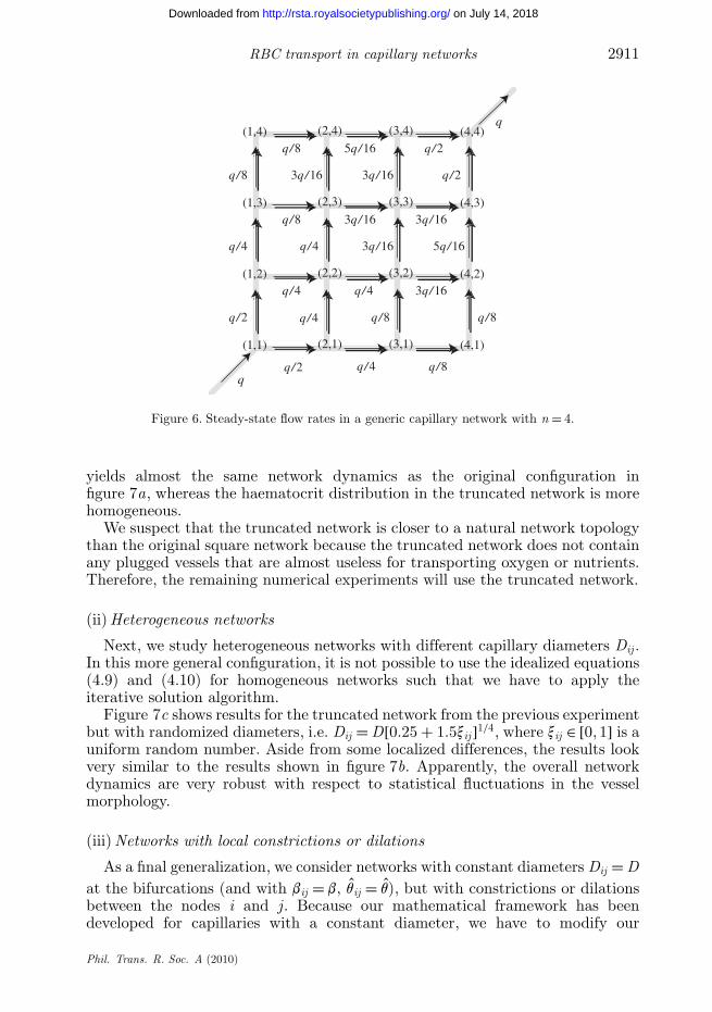
where dij is the Kronecker delta. The result of this algorithm for a network withn = 4 is illustrated in figure 6. It has been confirmed that the steady-state resultsfor the discrete RBC dynamics from §3 converge towards the continuous resultas the number of discrete RBCs increases.

Figure 7a shows the pressure field, mass flow rate, haematocrit and passivetracer distribution in a homogeneous 30 × 30 network with and without RBCs.As expected, we find that the pressure fields are the same up to a multiplicativeconstant. At the same time, we observe strong differences in the transportcharacteristics. The distribution of a passive tracer after the dimensionless timet = 0.4t illustrates these differences most clearly. Without RBCs, the tracer frontassumes roughly a circular shape. With RBCs, most of the tracer moves alonga preferential highway directly from the source to the sink. The haematocritdistribution is qualitatively the same as the distribution in the steady-stateconfiguration in figure 2d. The highest haematocrits are found in areas where theflow rates are small, i.e. a large fraction of the RBCs is used to ‘plug’ the networkin these places.

To illustrate this ‘plugging’, figure 7b shows results for a truncated network.In such a network, we eliminate all connections for which the effective resistanceis larger than a certain threshold. In other words, we assume that the capillarieswith high haematocrits are ‘plugged’ such that these capillaries might as wellbe omitted from the network. Surprisingly, we find that the truncated network





q

q

q/2

q/2

q/4

q/8

q/8

q/8

q/4 q/4

q/4

q/4

q/4

q/8

q/8

q/8 3q/16

3q/16

3q/16

3q/16

5q/16

5q/16

3q/16

3q/16 q/2

q/2

(1,1) (2,1) (3,1) (4,1)

(1,2) (2,2) (3,2) (4,2)

(1,3) (2,3) (3,3) (4,3)

(1,4) (2,4) (3,4) (4,4)

Figure 6. Steady-state flow rates in a generic capillary network with n = 4.

yields almost the same network dynamics as the original configuration infigure 7a, whereas the haematocrit distribution in the truncated network is morehomogeneous.

We suspect that the truncated network is closer to a natural network topologythan the original square network because the truncated network does not containany plugged vessels that are almost useless for transporting oxygen or nutrients.Therefore, the remaining numerical experiments will use the truncated network.

(ii) Heterogeneous networks

Next, we study heterogeneous networks with different capillary diameters Dij .In this more general configuration, it is not possible to use the idealized equations(4.9) and (4.10) for homogeneous networks such that we have to apply theiterative solution algorithm.

Figure 7c shows results for the truncated network from the previous experimentbut with randomized diameters, i.e. Dij = D[0.25 + 1.5xij ]1/4, where xij ∈ [0, 1] is auniform random number. Aside from some localized differences, the results lookvery similar to the results shown in figure 7b. Apparently, the overall networkdynamics are very robust with respect to statistical fluctuations in the vesselmorphology.

(iii) Networks with local constrictions or dilations

As a final generalization, we consider networks with constant diameters Dij = Dat the bifurcations (and with bij = b, qij = q), but with constrictions or dilationsbetween the nodes i and j . Because our mathematical framework has beendeveloped for capillaries with a constant diameter, we have to modify our





pressure f low rate(a)

(b)

(c)

(d )

haematocrit tracer at t = 0.4τ

horizontal dilation vertical dilationhorizontal and vertical

dilationhorizontal and vertical

constriction

Figure 7. Pressure, mass flow rate, haematocrit and passive tracer concentration at t = 0.4t ina 30 × 30 network (red, high values; blue, low values): (a) with (top row) and without RBCs(bottom row); (b) in a truncated network in which the capillaries with Re > 50R are eliminated;(c) truncated network with randomized diameters. The diagrams in (d) show the relative changein the haematocrit (top row) and flow rate (bottom row) for local constrictions/dilations in thecentre of the network.

network configuration. To this end, we split a capillary into three subsectionsby introducing two auxiliary nodes. The two outer sections have the diameter D,whereas the interior section of length L′ has the diameter D′ and an apparent





intrinsic viscosity b′. Each subsection can now be treated as a separate capillary.The application of the bifurcation rule at the auxiliary nodes is trivial becausethere is only a single capillary to choose from. It can even be shown thatequation (2.9), for computing the effective resistance, remains valid, albeit withmodified parameters Rij and bij . The effective resistance Re of the whole capillaryis given by

Re = Rij

(1 + Hij bij

), (4.11)

where Hij is the tube haematocrit in the unaltered vessel sections,

Rij =[Lij + L′

(D4

D′4 − 1

)]rij (4.12a)

and

bij =[

Lij + L′[(b′D2q)/(bD′2q′) − 1]Lij + L′(D4/D′4 − 1)

]bij . (4.12b)

With these modifications, we can use again the iterative solution algorithm tofind the steady-state solution of such networks. For the corresponding numericalexperiments, we use the truncated network and dilate or constrict capillaries inthe centre of the network.

Figure 7d shows the relative changes in the haematocrit (top row) and flowrate (bottom row) with respect to the truncated network shown in figure 7b. Westudy four different cases.

— Horizontal dilation. The diameter of the horizontal capillary in the centreof the network is increased such that the resulting specific resistance isreduced by 50 per cent.

— Vertical dilation. The diameter of the vertical capillary in the centre of thenetwork is increased such that the resulting specific resistance is reducedby 50 per cent.

— Horizontal and vertical dilation. The diameters of the horizontal and thevertical capillaries in the centre of the network are increased such thatboth specific resistances are reduced by 50 per cent.

— Horizontal and vertical constriction. The diameters of the horizontal andthe vertical capillaries in the centre of the network are decreased such thatboth specific resistances are doubled.

For the horizontal dilation (leftmost column in figure 7d), we find that thehaematocrit increases locally by more than 5 per cent to compensate for the lowerspecific resistance, i.e. there are more RBCs in the dilated capillary to ‘readjust’the effective resistance to its undilated value. At the same time, we find a regionjust above the dilated capillary with reduced haematocrit, which is probably dueto a local shortage of RBCs because of the higher RBC demand in the dilatedvessel. The mass flow rates change as well: there is a region of lower flow rate inthe wake of the dilated vessel and a region of increased flow rate on the oppositeside. Because of the symmetry of the network, the results for the vertical dilationare, of course, identical to those for the horizontal dilation, except that they aremirrored with respect to the main diagonal.





If we dilate the horizontal and the vertical vessels simultaneously (third columnin figure 7d), the wakes behind the dilations disappear. There is only a verylocalized increase in the haematocrit (and a small decrease in the neighbouringvessels). The flow rate is not noticeably affected by this dilation. For a constrictionof the horizontal and vertical vessels, we obtain the same result, but withopposite sign. Again, we find that local modifications lead to local changes inthe haematocrit and barely affect the flow rates.

5. Discussion and concluding remarks

We have presented a model for RBC transport in capillary networks, with a focuson the formulation of efficient algorithms and on the fundamental mechanisms ofthe network dynamics. We have shown that single-phase models for capillarynetworks lead to wrong results. The unphysiological build-up in the cornersof our generic network, for instance, would not be detected by a single-phaseKirchhoff approach. This finding is further supported by results as in figure 7a,which make it clear that the presence of RBCs in a capillary network has adramatic impact on the network dynamics. Figure 3 emphasizes the importanceof using a full model with a haematocrit-dependent flow resistance as well as abifurcation rule.

Of course, the proposed bifurcation rule may be questioned. Results byDesjardins & Duling (1987) suggest that the distribution of the dischargehaematocrit throughout a capillary network is quite homogeneous, whereas thevariations in the tube haematocrit are mostly due to an ESL rather than due tophase separation at bifurcations. If this were the case, we would need to replaceour bifurcation rule by a random bifurcation biased by the flow rate. Apartfrom the missing dynamical effects of the ESL (see the discussion in subsequentsections), we would then obtain results as in figure 3b. For the following reasons,however, we are confident that our bifurcation rule is appropriate: First, it isderived on the basis of strict physical arguments for a low Reynolds numberregime. Second, experimental observations at bifurcations (e.g. Fung 1973; Prieset al. 1989) are consistent with our numerical results. It can be regarded as asign of strength of the present formulation that it does not just duplicate theexperimentally observed behaviour by design, but that this behaviour follows asa result of the bifurcation rule.

An efficient model for the simulation of the fluid dynamics in themicrocirculation is particularly critical for the investigation of organs in whichthe level of perfusion is high. This can either be because the organ has ahigh metabolic rate (e.g. heart or brain) or is involved in the clearance ofmetabolites and toxins (e.g. liver and kidney). The impact of the presentmodel to study cerebral blood flow is evident. However, there are severalother fields where our model is relevant. In cancer therapy, for instance, adetailed understanding of the perfusion of densely vascularized tumours (Prieset al. 2009) is very important for general advances in tumour biology andan efficient administration of pharmaceuticals. The dynamics at bifurcationscan be used to design sophisticated filters (e.g. blood plasma separation;Yang et al. 2006).





(a) Limitations of the model

We have limited our studies to idealized square networks with a high level ofsymmetry. Certainly, it will be interesting to investigate the dynamics in moreirregular and realistic networks (e.g. Wieringa et al. 1982; Kassab et al. 1999).The local mechanisms (e.g. self-regulation) will also be found in these networks,but it is not clear per se what effect the local mechanisms will have on the globaldynamics of the whole network.

Further, the present formulation of the model neglects the distensibility ofthe vessels (Kassab et al. 1999) and the role of the ESL. The ESL interactswith the plasma and the blood particles, and has an influence on the localhaematocrit and flow resistance (Desjardins & Duling 1990; Vink & Duling 1996;Constantinescu et al. 2001). The effect of an ESL could be introduced to ourmodel by a velocity-dependent resistance of the RBC, i.e. the parameter r ij inequation (2.7) is then also a function of the RBC velocity uij . This will have aconsiderable impact on the transient dynamics of RBC transport. Nevertheless,the self-regulation mechanism will remain intact as long as the relations betweenthe intrinsic viscosity and the RBC velocity and the haematocrit are monotonic.Fig. 4 in Secomb et al. (2003) and fig. 4 in Pries & Secomb (2005), indicate thatthese relations are indeed monotonic. Therefore, we expect that the distributionof the flow rates in the steady-state configuration would remain unchanged (upto a constant multiplicative factor), whereas the haematocrit distribution wouldadapt to the changed conditions.

The present model neglects the presence of other blood particles apart fromRBCs. Possible implications of leucocytes on the RBC transport have beendiscussed by Schmid-Schönbein et al. (1980) with respect to the self-regulationmechanisms and by Han et al. (2006) with respect to the endothelial glycocalyx.

Although we believe that our formulation represents an appropriateidealization of the actual dynamics at a bifurcation, we would like to point outthat our bifurcation rule does not prevent an RBC from entering a capillary that isalready filled with RBCs. Such a situation can be found in diagram ① of figure 4,which shows more than 10 RBCs in a single capillary section of 50 mm length. Wecan prevent this from happening by adding another condition to the bifurcationrule that allows RBCs to enter a capillary only if Nij < Lij/Lij is satisfied. Wehave performed simulations with this modified bifurcation rule and found nofundamental differences in the presented results. We only noticed that the RBCdistribution is somewhat more homogeneous and that the ‘highway’ along themain diagonal is less pronounced.

(b) Relevance for the study of cerebral blood flow

A better knowledge of the cerebral microvascular system and the regulationof cerebral blood flow is fundamental for understanding the dynamics of manyphysiological and pathological processes in the brain. Furthermore, most ofthe functional neuroimaging methods, including the widely applied functionalmagnetic resonance imaging, rely on the haemodynamic response following neuralactivation. As a consequence, in order to correctly interpret the results of neuro-imaging experiments, mechanisms governing cerebral blood flow regulation mustbe well understood. Despite its small relative size, the brain uses approximately





one-quarter of the body’s total glucose turnover and about one-fifth of the oxygen.The continuous delivery of oxygen is particularly critical and already temporaryshortages can lead to transient failures or irreversible damage of nervous tissue.The present study provides the basis for studying oxygen transfer from blood totissue, particularly when applied to realistic vascular networks. More specifically,the haematocrit and RBC residence time fundamentally determine the tissueoxygen extraction. Recent studies have demonstrated that pericyte constrictionscan regulate vascular resistance on the capillary level (Peppiatt et al. 2006;Yemisci et al. 2009). Our simulations provide first evidence that the effect ofa local increase in capillary diameter is a concomitant increase in the localhaematocrit. Recent advances in high-resolution imaging (e.g. two-photon laserscanning microscopy) should be exploited to confirm this result in vivo. Anotherinteresting finding is the fact that RBC flow stagnates in specific areas of ourartificial network. When looking at this phenomenon from a developmentalviewpoint, it becomes evident that the vascular topology undergoes a kind ofselection process. Flow in ‘inefficient’ capillaries would stall and would eventuallylead to the degeneration of these vessels. In fact, there is evidence from histologicalstudies that capillaries do indeed degenerate, which results in basal membraneremnants known as ‘string vessels’ (Challa et al. 2002).

The presented model for RBC transport in capillary networks is a buildingblock for a comprehensive model of human physiology. In such a framework, themodel can serve as an algorithmic tool for simulating blood flow in a spatiallyresolved capillary network. It can be linked through in- and outflow boundaryconditions to a model for flow in larger blood vessels. The link to the perfusedorgan is established through the haematocrit distribution (oxygen supply) and/orthrough a passive tracer distribution (e.g. glucose concentration). Alternatively,the model may be used in a multi-scale approach where basic results for thenetwork dynamics are upscaled to a next higher level of spatial abstraction. Inthat sense, numerical results for isolated prototypical networks (e.g. figure 7)could be used to estimate the permeability tensor for Darcy’s law (Reichold et al.2009), such that capillaries can be treated as a spatial continuum between largerblood vessels.

References

Albrecht, K. H., Gaehtgens, P., Pries, A. & Heuser, M. 1979 The Fahraeus effect innarrow capillaries (i.d. 3.3 to 11.0 micron). Microvasc. Res. 18, 33–47. (doi:10.1016/0026-2862(79)90016-5)

Barber, J. O., Alberding, J. P., Restrepo, J. M. & Secomb, T. W. 2008 Simulated two-dimensionalred blood cell motion, deformation, and partitioning in microvessel bifurcations. Ann. Biomed.Eng. 36, 1690–1698. (doi:10.1007/s10439-008-9546-4)

Boas, D. A., Jones, S. R., Devor, A., Huppert, T. J. & Dale A. M. 2008 A vascular anatomicalnetwork model of the spatio-temporal response to brain activation. NeuroImage 40, 1116–1129.(doi:10.1016/j.neuroimage.2007.12.061)

Challa, V. R., Thore, C. R., Moody, D. M., Brown, W. R. & Anstrom, J. A. 2002 A three-dimensional study of brain string vessels using celloidin sections stained with anti-collagenantibodies. J. Neurol. Sci. 203–204, 165–167. (doi:10.1016/S0022-510X(02)00284-8)

Constantinescu, A. A., Vink, H. & Spaan, J. A. E. 2001 Elevated capillary tube hematocrit reflectdegradation of endothelial cell glycocalyx by oxidized LDL. Am. J. Physiol. Heart. Circ. Physiol.280, H1051–H1057.



http://dx.doi.org/doi:10.1016/0026-2862(79)90016-5


http://dx.doi.org/doi:10.1007/s10439-008-9546-4

http://dx.doi.org/doi:10.1016/j.neuroimage.2007.12.061

http://dx.doi.org/doi:10.1016/S0022-510X(02)00284-8



Dawant, B., Levin, M. & Popel, A. S. 1986a Effect of dispersion of vessel diameters and lengthsin stochastic networks: I. Modeling of microcirculatory flow. Microvasc. Res. 31, 203–222.(doi:10.1016/0026-2862(86)90035-X)

Dawant, B., Levin, M. & Popel, A. S. 1986b Effect of dispersion of vessel diameters and lengths instochastic networks: II. Modeling of microvascular hematocrit distribution. Microvasc. Res. 31,223–234. (doi:10.1016/0026-2862(86)90035-X)

Desjardins, C. & Duling, B. R. 1987 Microvessel hematocrit: measurement and implications forcapillary oxygen transport. Am. J. Physiol. Heart Circ. Physiol. 252, H494–H503.

Desjardins, C. & Duling, B. R. 1990 Heparinase treatment suggests a role for the endothelialcell glycocalyx in regulation of capillary hematocrit. Am. J. Physiol. Heart Circ. Physiol. 258,H647–H654.

Fung, Y. C. 1973 Stochastic flow in capillary blood vessels. Microvasc. Res. 5, 34–48. (doi:10.1016/S0026-2862(73)80005-6)

Han, Y., Weinbaum, S., Spaan, J. A. E. & Vink, H. 2006 Large-deformation analysis of the elasticrecoil of fibre layers in a Brinkman medium with application to the endothelial glycocalyx.J. Fluid. Mech. 554, 217–235. (doi:10.1017/S0022112005007779)

Kassab, G. S., Le, K. N. & Fung, Y.-C. B. 1999 A hemodynamic analysis of coronary capillaryblood flow based on anatomic and distensibility data. Am. J. Physiol. Heart Circ. Physiol. 277,2158–2166.

Kleinfeld, D., Mitra, P. P., Helmchen, F. & Denk, W. 1998 Fluctuations and stimulus-inducedchanges in blood flow observed in individual capillaries in layers 2 through 4 of rat neocortex.Proc. Natl Acad. Sci. USA 95, 15 741–15 746. (doi:10.1073/pnas.95.26.15741)

Klitzman, B. & Johnson, P. C. 1982 Capillary network geometry and red cell distribution in hamstercremaster muscle. Am. J. Physiol. Heart Circ. Physiol. 242, H211–H219.

Lawrence, M. & Clapper, M. P. 1972 Analysis of flow pattern in vas spirale. Acta Otolaryngol. 73,94–103. (doi:10.3109/00016487209138917)

Papenfuss, H.-D. & Gross, J. F. 1981 Microhemodynamics of capillary networks. Biorheology 18,673–692.

Peppiatt, C., Howarth, C., Mobbs, P. & Attwell, D. 2004 Bidirectional control of CNS capillarydiameter by pericytes. Nature 443, 700–704. (doi:10.1038/nature05193)

Pozrikidis, C. 2003 Numerical simulation of the flow-induced deformation of red blood cells. Ann.Biomed. Eng. 31, 1194–1205. (doi:10.1114/1.1617985)

Pozrikidis, C. 2005a Axisymmetric motion of a file of red blood cells through capillaries. Phys.Fluids 17, 031503. (doi:10.1063/1.1830484)

Pozrikidis, C. 2005b Numerical simulation of cell motion in tube flow. Ann. Biomed. Eng. 33,165–178. (doi:10.1007/s10439-005-8975-6)

Pries, A. R. & Secomb, T. W. 2005 Microvascular blood viscosity in vivo and the endothelialsurface layer. Am. J. Physiol. Heart Circ. Physiol. 289, H2657–H2664. (doi:10.1152/ajpheart.00297.2005)

Pries, A. R., Ley, K. & Gaehtgens, P. 1986 Generalization of the fahraeus principle for microvesselnetworks. Am. J. Physiol. Heart Circ. Physiol. 251, H1324–H1332.

Pries, A. R., Ley, K., Claasen, M. & von Gaehtgens, M. 1989 Red cell distribution at microvascularbifurcations. Microvasc. Res. 38, 81–101. (doi:10.1016/0026-2862(89)90018-6)

Pries, A. R., Secomb, T. W., Gaehtgens, P. & Gross, J. F. 1990 Blood flow in microvascularnetworks. Experiments and simulation. Circ. Res. 67, 826–834.

Pries, A. R., Fritzsche, A., Ley, K. & Gaehtgens, P. 1992 Redistribution of red blood cell flow inmicrocirculatory networks by hemodilution. Circ. Res. 70, 1113–1121.

Pries, A. R., Cornelissen, A. J. M., Sloot, A. A., Hinkeldey, M., Dreher, M. R., Höpfner, M.,Dewhirst, M. W. & Secomb, T. W. 2009 Structural adaptation and heterogeneity of normaland tumor microvascular networks. PLoS Comput. Biol. 5, e1000394. (doi:10.1371/journal.pcbi.1000394)

Reichold, J., Stampanoni, M., Keller, A. L., Buck, A., Jenny, P. & Weber, B. 2009 Vascular graphmodel to simulate the cerebral blood flow in realistic vascular networks. J. Cereb. Blood FlowMetab. 29, 1429–1443. (doi:10.1038/jcbfm.2009.58)



http://dx.doi.org/doi:10.1016/0026-2862(86)90035-X

http://dx.doi.org/doi:10.1016/0026-2862(86)90035-X

http://dx.doi.org/doi:10.1016/S0026-2862(73)80005-6

http://dx.doi.org/doi:10.1016/S0026-2862(73)80005-6

http://dx.doi.org/doi:10.1017/S0022112005007779

http://dx.doi.org/doi:10.1073/pnas.95.26.15741

http://dx.doi.org/doi:10.3109/00016487209138917

http://dx.doi.org/doi:10.1038/nature05193

http://dx.doi.org/doi:10.1114/1.1617985


http://dx.doi.org/doi:10.1007/s10439-005-8975-6

http://dx.doi.org/doi:10.1152/ajpheart.00297.2005

http://dx.doi.org/doi:10.1152/ajpheart.00297.2005


http://dx.doi.org/doi:10.1371/journal.pcbi.1000394

http://dx.doi.org/doi:10.1371/journal.pcbi.1000394

http://dx.doi.org/doi:10.1038/jcbfm.2009.58



Schmid-Schönbein, G. W., Skalak, R., Usami, S. & Chien, S. 1980 Cell distribution in capillarynetworks. Microvasc. Res. 19, 18–44. (doi:10.1016/0026-2862(80)90082-5)

Secomb, T. W. & Hsu, R. 1996 Motion of red blood cells in capillaries with variable cross-sections.J. Biomech. Eng. 118, 538–544. (doi:10.1115/1.2796041)

Secomb, T. W., Skalak, R., Özkaya, N. & Gross, J. F. 1986 Flow of axisymmetric red blood cellsin narrow capillaries. J. Fluid. Mech. 163, 405–423. (doi:10.1017/S0022112086002355)

Secomb, T. W., Pries, A. R. & Gaehtgens, P. 1995 Architecture and hemodynamics of microvascularnetworks. In Biological flows (eds M. Y. Jaffrin & C. Caro), pp. 159–176. New York, NY: PlenumPress.

Secomb, T. W., Hsu, R. & Pries, A. R. 2003 Motion of red blood cells in a capillary with anendothelial surface layer: effect of flow velocity. Am. J. Physiol. Heart Circ. Physiol. 281, H629–H636.

Sutera, S. P. & Skalak, R. 1993 The history of Poiseuille’s law. Annu. Rev. Fluid Mech. 25, 1–20.(doi:10.1146/annurev.fl.25.010193.000245)

Tsai, P., Kaufhold, J. P., Blinder, P., Friedman, B., Drew P. J., Karten, H. J., Lyden, P. D. &Kleinfeld, D. 2009 Correlations of neuronal and microvascular densities in murine cortex revealedby direct counting and colocalization of nuclei and vessels. J. Neurosci. 29, 14 553–14 570.(doi:10.1523/jneurosci.3287-09.2009)

Vink, H. & Duling, B. R. 1996 Identification of distinct luminal domains for macromolecules,erythrocytes, and leukocytes within mammalian capillaries. Circ. Res. 79, 581–589.

Wieringa, P. A., Spaan, J. A. E., Stasse, H. G. & Laird, J. D. 1982 Heterogeneous flow distributionin a three dimensional network simulation of the myocardial microcirculation—a hypothesis.Microcirculation 2, 195–216.

Yang, S., Ündar, A. & Zahn, J. 2006 A microfluidic device for continuous, real time blood plasmaseparation. Lab. Chip 6, 871–880. (doi:10.1039/b516401j)

Yemisci, M., Gursoy-Ozdemir, Y., Vural, A., Can, A., Topalkara, K. & Dalkara, T. 2009 Pericytecontraction induced by oxidative-nitrative stress impairs capillary reflow despite successfulopening of an occluded cerebral artery. Nat. Med. 15, 1031–1073. (doi:10.1038/nm.2022)





http://dx.doi.org/doi:10.1017/S0022112086002355

http://dx.doi.org/doi:10.1146/annurev.fl.25.010193.000245

http://dx.doi.org/doi:10.1523/jneurosci.3287-09.2009

http://dx.doi.org/doi:10.1039/b516401j

http://dx.doi.org/doi:10.1038/nm.2022


red blood cell distribution in simpliﬁed capillary...

Documents