recursive teaching dimension, vc-dimension and sample...

Journal of Machine Learning Research 15 (2014) 3107-3131 Submitted 1/13; Revised 5/14; Published 10/14

Recursive Teaching Dimension, VC-Dimension and SampleCompression

Thorsten Doliwa [email protected] of MathematicsRuhr-Universität Bochum, D-44780 Bochum, Germany

Gaojian Fan [email protected] of Computing ScienceUniversity of Alberta, Edmonton, AB, T6G 2E8, Canada

Hans Ulrich Simon [email protected]örtz Institute for IT Security and Faculty of MathematicsRuhr-Universität Bochum, D-44780 Bochum, Germany

Sandra Zilles [email protected] of Computer ScienceUniversity of Regina, Regina, SK, S4S 0A2, Canada

Editor: Manfred Warmuth

AbstractThis paper is concerned with various combinatorial parameters of classes that can be learnedfrom a small set of examples. We show that the recursive teaching dimension, recentlyintroduced by Zilles et al. (2008), is strongly connected to known complexity notions inmachine learning, e.g., the self-directed learning complexity and the VC-dimension. To thebest of our knowledge these are the first results unveiling such relations between teachingand query learning as well as between teaching and the VC-dimension. It will turn outthat for many natural classes the RTD is upper-bounded by the VCD, e.g., classes of VC-dimension 1, intersection-closed classes and finite maximum classes. However, we will alsoshow that there are certain (but rare) classes for which the recursive teaching dimensionexceeds the VC-dimension. Moreover, for maximum classes, the combinatorial structureinduced by the RTD, called teaching plan, is highly similar to the structure of samplecompression schemes. Indeed one can transform any repetition-free teaching plan for amaximum class C into an unlabeled sample compression scheme for C and vice versa, whilethe latter is produced by (i) the corner-peeling algorithm of Rubinstein and Rubinstein(2012) and (ii) the tail matching algorithm of Kuzmin and Warmuth (2007).Keywords: recursive teaching, combinatorial parameters, Vapnik-Chervonenkis dimen-sion, upper bounds, compression schemes, tail matching algorithm

1. Introduction

In the design and analysis of machine learning algorithms, the amount of training datathat needs to be provided for the learning algorithm to be successful is an aspect of central

c©2014 Thorsten Doliwa, Gaojian Fan, Hans Ulrich Simon and Sandra Zilles.

Doliwa, Fan, Simon and Zilles

importance. In many applications, training data is expensive or difficult to obtain, andthus input-efficient learning algorithms are desirable. In computational learning theorytherefore, one way of measuring the complexity of a concept class is to determine the worst-case number of input examples required by the best valid learning algorithm. What is avalid learning algorithm depends on the underlying model of learning. We refer to this kindof complexity measure as information complexity. For example, in PAC-learning (Valiant,1984), the information complexity of a concept class C is the worst-case sample complexity abest possible PAC learner for C can achieve on all concepts in C. In query learning (Angluin,1988), it is the best worst-case number of queries a learner would have to ask to identifyan arbitrary concept in C. In the classical model of teaching (Goldman and Kearns, 1995;Shinohara and Miyano, 1991), the information complexity of C is given by its teachingdimension, i.e., the largest number of labeled examples that would have to be provided fordistinguishing any concept in C from all other concepts in C.

Besides the practical need to limit the required amount of training data, there are anumber of reasons for formally studying information complexity. Firstly, a theoretical studyof information complexity yields formal guarantees concerning the amount of data that needsto be processed to solve a learning problem. Secondly, analyzing information complexityoften helps to understand the structural properties of concept classes that are particularlyhard to learn or particularly easy to learn. Thirdly, the theoretical study of informationcomplexity helps to identify connections between various formal models of learning, forexample if it turns out that, for a certain type of concept class, the information complexityunder learning model A is in some relationship with the information complexity under modelB. This third aspect is the main motivation of our study.

In the past two decades, several learning models were defined with the aim of under-standing in which way a low information complexity can be achieved. One such model islearning from partial equivalence queries (Maass and Turán, 1992), which subsume all typesof queries for which negative answers are witnessed by counterexamples, e.g., membership,equivalence, subset, superset, and disjointness queries (Angluin, 1988). As lower bounds onthe information complexity in this query model (here called query complexity) hold for nu-merous other query learning models, they are particularly interesting objects of study. Evenmore powerful are self-directed learners (Goldman et al., 1993). Each query of a self-directedlearner is a prediction of a label for an instance of the learner’s choice, and the learner getscharged only for wrong predictions. The query complexity in this model lower-bounds theone obtained from partial equivalence queries (Goldman and Sloan, 1994).

Dual to the models of query learning, in which the learner actively chooses the instancesit wants information on, the literature proposes models of teaching (Goldman and Kearns,1995; Shinohara and Miyano, 1991), in which a helpful teacher selects a set of examples andpresents it to the learner, again aiming at a low information complexity. A recent modelof teaching with low information complexity is recursive teaching, where a teacher choosesa sample based on a sequence of nested subclasses of the underlying concept class C (Zilleset al., 2008). The nesting is defined as follows. The outermost “layer” consists of all conceptsin C that are easiest to teach, i.e., that have the smallest sets of examples distinguishingthem from all other concepts in C. The next layers are formed by recursively repeatingthis process with the remaining concepts. The largest number of examples required forteaching at any layer is the recursive teaching dimension (RTD) of C. The RTD substantially

3108

Recursive Teaching Dimension, VC-Dimension and Sample Compression

reduces the information complexity bounds obtained in previous teaching models. It lowerbounds not only the teaching dimension—the measure of information complexity in the“classical” teaching model (Goldman and Kearns, 1995; Shinohara and Miyano, 1991)—butalso the information complexity of iterated optimal teaching (Balbach, 2008), which is oftensubstantially smaller than the classical teaching dimension.

A combinatorial parameter of central importance in learning theory is the VC-dimen-sion (Vapnik and Chervonenkis, 1971). Among many relevant properties, it provides boundson the sample complexity of PAC-learning (Blumer et al., 1989). Since the VC-dimensionis the best-studied quantity related to information complexity in learning, it is a naturalfirst parameter to compare to when it comes to identifying connections between informa-tion complexity notions across various models of learning. For example, even though theself-directed learning complexity can exceed the VC-dimension, existing results show someconnection between these two complexity measures (Goldman and Sloan, 1994). However,the teaching dimension, i.e., the information complexity of the classical teaching model,does not exhibit any general relationship to the VC-dimension—the two parameters can bearbitrarily far apart in either direction (Goldman and Kearns, 1995). Similarly, there is noknown connection between teaching dimension and query complexity.

In this paper, we establish the first known relationships between the information com-plexity of teaching and query complexity, as well as between the information complexity ofteaching and the VC-dimension. All these relationships are exhibited by the RTD. Two ofthe main contributions of this work are the following:

• We show that the RTD is never higher (and often considerably lower) than the com-plexity of self-directed learning. Hence all lower bounds on the RTD hold likewise forself-directed learning, for learning from partial equivalence queries, and for a varietyof other query learning models.

• We reveal a strong connection between the RTD and the VC-dimension. Thoughthere are classes for which the RTD exceeds the VC-dimension, we present a numberof quite general and natural cases in which the RTD is upper-bounded by the VC-dimension. These include classes of VC-dimension 1, intersection-closed classes, avariety of naturally structured Boolean function classes, and finite maximum classesin general (i.e., classes of maximum possible cardinality for a given VC-dimension anddomain size). Many natural concept classes are maximum, e.g., the class of unionsof up to k intervals, for any k ∈ N, or the class of simple arrangements of positivehalfspaces. It remains open whether every class of VC-dimension d has an RTD linearin d.

In proving that the RTD of a finite maximum class equals its VC-dimension, we also makea third contribution:

• We reveal a relationship between the RTD and sample compression schemes (Little-stone and Warmuth, 1996).

Sample compression schemes are schemes for “encoding” a set of examples in a small subsetof examples. For instance, from the set of examples they process, learning algorithms oftenextract a subset of particularly “significant” examples in order to represent their hypotheses.

3109


This way sample bounds for PAC-learning of a class C can be obtained from the size ofa smallest sample compression scheme for C (Littlestone and Warmuth, 1996; Floyd andWarmuth, 1995). Here the size of a scheme is the size of the largest subset resulting fromcompression of any sample consistent with some concept in C.

The relationship between RTD and unlabeled sample compression schemes (in whichthe compression sets consist only of instances without labels) is established via a recentresult by Rubinstein and Rubinstein (2012). They show that, for any maximum class of VC-dimension d, a technique called corner-peeling defines unlabeled compression schemes of sized. Like the RTD, corner-peeling is associated with a nesting of subclasses of the underlyingconcept class. A crucial observation we make in this paper is that every maximum classof VC-dimension d allows corner-peeling with an additional property, which ensures thatthe resulting unlabeled samples contain exactly those instances a teacher following the RTDmodel would use. Similarly, we show that the unlabeled compression schemes constructedby Kuzmin and Warmuth’s Tail Matching algorithm (Kuzmin and Warmuth, 2007) exactlycoincide with the teaching sets used in the RTD model, all of which have size at most d.

This remarkable relationship between the RTD and sample compression suggests thatthe open question of whether or not the RTD is linear in the VC-dimension might be relatedto the long-standing open question of whether or not the best possible size of sample com-pression schemes is linear in the VC-dimension, cf. (Littlestone and Warmuth, 1996; Floydand Warmuth, 1995). To this end, we observe that a negative answer to the former ques-tion would have implications on potential approaches to settling the second. In particular,if the RTD is not linear in the VC-dimension, then there is no mapping that maps everyconcept class of VC-dimension d to a superclass that is maximum of VC-dimension O(d).Constructing such a mapping would be one way of proving that the best possible size ofsample compression schemes is linear in the VC-dimension.

Note that sample compression schemes are not bound to any constraints as to howthe compression sets have to be formed, other than that they be subsets of the set tobe compressed. In particular, any kind of agreement on, say, an order over the instancespace or an order over the concept class, can be exploited for creating the smallest possiblecompression scheme. As opposed to that, the RTD is defined following a strict “recipe”in which teaching sets are independent of orderings of the instance space or the conceptclass. These differences between the models make the relationship revealed in this papereven more remarkable. Further connections between teaching and sample compression canin fact be obtained when considering a variant of the RTD introduced by Darnstädt et al.(2013). This new teaching complexity parameter upper-bounds not only the RTD and theVC-dimension, but also the smallest possible size of a sample compression scheme for theunderlying concept class. Darnstädt et al. (2013) dubbed this parameter order compressionnumber, as it corresponds to the smallest possible size of a special form of compressionscheme called order compression scheme of the class.

This paper is an extension of an earlier publication (Doliwa et al., 2010).

2. Definitions, Notation and Facts

Throughout this paper, X denotes a finite set and C denotes a concept class over domainX. For X ′ ⊆ X, we define C|X′ := C ∩ X ′| C ∈ C. We treat concepts interchangeably

3110


as subsets of X and as 0, 1-valued functions on X. A labeled example is a pair (x, l) withx ∈ X and l ∈ 0, 1. If S is a set of labeled examples, we define X(S) = x ∈ X | (x, 0) ∈S or (x, 1) ∈ S. For brevity, [n] := 1, . . . , n. VCD(C) denotes the VC-dimension of aconcept class C.

Definition 1 Let K be a function that assigns a “complexity” K(C) ∈ N to each conceptclass C. We say that K is monotonic if C′ ⊆ C implies that K(C′) ≤ K(C). We say thatK is twofold monotonic if K is monotonic and, for every concept class C over X and everyX ′ ⊆ X, it holds that K(C|X′) ≤ K(C).

2.1 Learning Complexity

A partial equivalence query (Maass and Turán, 1992) of a learner is given by a functionh : X → 0, 1, ∗ that is passed to an oracle. The latter returns “YES” if the targetconcept C∗ coincides with h on all x ∈ X for which h(x) ∈ 0, 1; it returns a “witness ofinequivalence” (i.e., an x ∈ X such that C∗(x) 6= h(x) ∈ 0, 1) otherwise. LC-PARTIAL(C)denotes the smallest number q such that there is some learning algorithm which can exactlyidentify any concept C∗ ∈ C with up to q partial equivalence queries (regardless of theoracle’s answering strategy).

A query in the model of self-directed learning (Goldman et al., 1993; Goldman and Sloan,1994) consists of an instance x ∈ X and a label b ∈ 0, 1, passed to an oracle. The latterreturns the true label C∗(x) assigned to x by the target concept C∗. We say the learnermade a mistake if C∗(x) 6= b. The self-directed learning complexity of C, denoted SDC(C),is defined as the smallest number q such that there is some self-directed learning algorithmwhich can exactly identify any concept C∗ ∈ C without making more than q mistakes.

In the model of online-learning, the learner A makes a prediction bi ∈ 0, 1 for a giveninstance xi but, in contrast to self-directed learning, the sequence of instances x1, x2, . . .is chosen by an adversary of A that aims at maximizing A’s number of mistakes. Theoptimal mistake bound for a concept class C, denoted Mopt(C), is the smallest number qsuch that there exists an online-learning algorithm which which can exactly identify anyconcept C∗ ∈ C without making more than q mistakes (regardless of the ordering in whichthe instances are presented to A).

Clearly, LC-PARTIAL and SDC are monotonic, and Mopt is twofold monotonic. Thefollowing chain of inequalities is well-known (Goldman and Sloan, 1994; Maass and Turán,1992; Littlestone, 1988):

SDC(C) ≤ LC-PARTIAL(C) ≤Mopt(C) ≤ log |C| . (1)

2.2 Teaching Complexity

A teaching set for a concept C ∈ C is a set S of labeled examples such that C, but noother concept in C, is consistent with S. Let T S(C, C) denote the family of teaching sets for

3111


C ∈ C, let TS(C; C) denote the size of the smallest teaching set for C ∈ C, and let

TSmin(C) := minC∈C

TS(C; C) ,

TSmax(C) := maxC∈C

TS(C; C) ,

TSavg(C) :=1

|C|∑C∈C

TS(C; C) .

The quantity TD(C) := TSmax(C) is called the teaching dimension of C (Goldman andKearns, 1995). It refers to the concept in C that is hardest to teach. In the sequel, TSmin(C)is called the best-case teaching dimension of C, and TSavg(C) is called the average-caseteaching dimension of C. Obviously, TSmin(C) ≤ TSavg(C) ≤ TSmax(C) = TD(C).

We briefly note that TD is monotonic, and that a concept class C consisting of exactlyone concept C has teaching dimension 0 because ∅ ∈ T S(C, C).

Definition 2 (Zilles et al. 2011) A teaching plan for C is a sequence

P = ((C1, S1), . . . , (CN , SN )) (2)

with the following properties:

• N = |C| and C = C1, . . . , CN.

• For all t = 1, . . . , N , St ∈ T S(Ct, Ct, . . . , CN).

The quantity ord(P ) := maxt=1,...,N |St| is called the order of the teaching plan P . Finally,we define

RTD(C) := minord(P ) | P is a teaching plan for C ,RTD∗(C) := max

X′⊆XRTD(C|X′) .

The quantity RTD(C) is called the recursive teaching dimension of C.

A teaching plan (2) is said to be repetition-free if the sets X(S1), . . . , X(SN ) are pairwisedistinct. (Clearly, the corresponding labeled sets, S1, . . . , SN , are always pairwise distinct.)Similar to the recursive teaching dimension we define

rfRTD(C) := minord(P ) | P is a repetition-free teaching plan for C .

One can show that every concept class possesses a repetition-free teaching plan. First,by induction on |X| = m, the full cube 2X has a repetition-free teaching plan of order m:It results from a repetition-free plan for the (m − 1)-dimensional subcube of concepts forwhich a fixed instance x is labeled 1, where each teaching set is supplemented by the example(x, 1), followed by a repetition-free teaching plan for the (m − 1)-dimensional subcube ofconcepts with x = 0. Second, “projecting” a (repetition-free) teaching plan for a conceptclass C onto the concepts in a subclass C′ ⊆ C yields a (repetition-free) teaching plan for C′.Putting these two observations together, it follows that every class over instance set X hasa repetition-free teaching plan of order |X|.

3112


x1 x2 x3 x4 x5 TSmin TSmin(Ci,C\C1) TSmin(Ci,C\C2) TSmin(Ci,C\C1/2)

C1 0 0 0 0 0 2 - 2 -C2 1 1 0 0 0 2 2 - -C3 0 1 0 0 0 4 3 3 2C4 0 1 0 1 0 4 4 4 4C5 0 1 0 1 1 3 3 3 3C6 0 1 1 1 0 3 3 3 3C7 0 1 1 0 1 3 3 3 3C8 0 1 1 1 1 3 3 3 3C9 1 0 1 0 0 3 3 3 3C10 1 0 0 1 0 4 3 3 3C11 1 0 0 1 1 3 3 3 3C12 1 0 1 1 0 3 3 3 3C13 1 0 1 0 1 3 3 3 3

Table 1: A class with RTD(C) = 2 but rfRTD(C) = 3.

It should be noted though that rfRTD(C) may exceed RTD(C). For example, considerthe class in Table 1, which is of RTD 2. In any teaching plan of order 2, both C1 and C2

have to be taught first with the same teaching set x1, x2 augmented by the appropriatelabels. The best repetition free teaching plan for this class is of order 3.

As observed by Zilles et al. (2011), the following holds:

• RTD is monotonic.

• The recursive teaching dimension coincides with the order of any teaching plan thatis in canonical form, i.e., a teaching plan ((C1, S1), . . . , (CN , SN )) such that for allt = 1, . . . , N it holds that |St| = TSmin(Ct, . . . , CN).

Intuitively, a canonical teaching plan is a sequence that is recursively built by always pickingan easiest-to-teach concept Ct in the class C \ C1, . . . , Ct−1 together with an appropriateteaching set St.

The definition of teaching plans immediately yields the following result:

Lemma 3 1. If K is monotonic and TSmin(C) ≤ K(C) for every concept class C, thenRTD(C) ≤ K(C) for every concept class C.

2. If K is twofold monotonic and TSmin(C) ≤ K(C) for every concept class C, thenRTD∗(C) ≤ K(C) for every concept class C.

RTD and TSmin are related as follows:

Lemma 4 RTD(C) = maxC′⊆C TSmin(C′).

Proof Let C1 be the first concept in a canonical teaching plan P for C so that TS(C1; C) =TSmin(C) and the order of P equals RTD(C). It follows that

RTD(C) = maxTS(C1; C),RTD(C \ C1) = maxTSmin(C),RTD(C \ C1) ,

3113


and RTD(C) ≤ maxC′⊆C TSmin(C′) follows inductively. As for the reverse direction, letC′0 ⊆ C be a maximizer of TSmin. Since RTD is monotonic, we get RTD(C) ≥ RTD(C′0) ≥TSmin(C′0) = maxC′⊆C TSmin(C′).

2.3 Intersection-closed Classes and Nested Differences

A concept class C is called intersection-closed if C ∩ C ′ ∈ C for all C,C ′ ∈ C. Among thestandard examples of intersection-closed classes are the d-dimensional boxes over domain[n]d:

BOXdn := [a1 : b1]× · · · × [ad : bd] | ∀i = 1, . . . , d : 1 ≤ ai, bi ≤ n

Here, [a : b] is an abbreviation for a, a + 1, . . . , b, where [a : b] is the empty set if a > b.For the remainder of this section, C is assumed to be intersection-closed.

For T ⊆ X, we define 〈T 〉C as the smallest concept in C containing T , i.e.,

〈T 〉C :=⋂

T⊆C∈CC .

A spanning set for T ⊆ X w.r.t. C is a set S ⊆ T such that 〈S〉C = 〈T 〉C . S is called aminimal spanning set w.r.t. C if, for every proper subset S′ of S, 〈S′〉C 6= 〈S〉C . I(C) denotesthe size of the largest minimal spanning set w.r.t. C. It is well-known (Natarajan, 1987;Helmbold et al., 1990) that every minimal spanning set w.r.t. C is shattered by C. Thus,I(C) ≤ VCD(C). Note that, for every C ∈ C, I(C|C) ≤ I(C), because every spanning setfor a set T ⊆ C w.r.t. C is also a spanning set for T w.r.t. C|C .

The class of nested differences of depth d (at most d) with concepts from C, denotedDIFFd(C) (DIFF≤d(C), resp.), is defined inductively as follows:

DIFF1(C) := C ,DIFFd(C) := C \D | C ∈ C, D ∈ DIFFd−1(C) ,

DIFF≤d(C) :=d⋃

i=1

DIFFi(C) .

Expanding the recursive definition of DIFFd(C) shows that, e.g., a set in DIFF4(C) has theform C1\(C2\(C3\C4)) where C1, C2, C3, C4 ∈ C. We may assume without loss of generalitythat C1 ⊇ C2 ⊇ · · · because C is intersection-closed.

Nested differences of intersection-closed classes were studied in depth at the early stagesof research in computational learning theory (Helmbold et al., 1990).

2.4 Maximum Classes and Unlabeled Compression Schemes

Let Φd(n) :=∑d

i=0

(ni

). For d = VCD(C) and for any subset X ′ of X, we have

∣∣C|X′∣∣ ≤Φd(|X ′|), according to Sauer’s Lemma (Vapnik and Chervonenkis, 1971; Sauer, 1972). Theconcept class C is called a maximum class if Sauer’s inequality holds with equality for everysubset X ′ of X. It is well-known (Welzl, 1987; Floyd and Warmuth, 1995) that a class overa finite domain X is maximum iff Sauer’s inequality holds with equality for X ′ = X.

The following definition was introduced by Kuzmin and Warmuth (2007):

3114


Definition 5 An unlabeled compression scheme for a maximum class of VC-dimension d isgiven by an injective mapping r that assigns to every concept C a set r(C) ⊆ X of size atmost d such that the following condition is satisfied:

∀C,C ′ ∈ C (C 6= C ′),∃x ∈ r(C) ∪ r(C ′) : C(x) 6= C ′(x) . (3)

(3) is referred to as the non-clashing property. In order to ease notation, we add the followingtechnical definitions. A representation mapping of order k for a (not necessarily maximum)class C is any injective mapping r that assigns to every concept C a set r(C) ⊆ X ofsize at most k such that (3) holds. A representation-mapping r is said to have the acyclicnon-clashing property if there is an ordering C1, . . . , CN of the concepts in C such that

∀1 ≤ i < j ≤ N, ∃x ∈ r(Ci) : Ci(x) 6= Cj(x) . (4)

Considering maximum classes, it was shown by Kuzmin and Warmuth (2007) that arepresentation mapping with the non-clashing property guarantees that, for every sample Slabeled according to a concept in C, there is exactly one concept C ∈ C that is consistentwith S and satisfies r(C) ⊆ X(S). This allows to encode (compress) a labeled sample S byr(C) and, since r is injective, to decode (decompress) r(C) by C (so that the labels in Scan be reconstructed). This coined the term “unlabeled compression scheme”.

A concept class C over a domain X of size n is identified with a subset of 0, 1n. Theone-inclusion-graph G(C) associated with C is defined as follows:

• The nodes are the concepts from C.

• Two concepts are connected by an edge if and only if they differ in exactly one coor-dinate (when viewed as nodes in the Boolean cube).

A cube C′ in C is a subcube of 0, 1n such that every node in C′ represents a concept from C.In the context of the one-inclusion graph, the instances (corresponding to the dimensions inthe Boolean cube) are usually called “colors” (and an edge along dimension i is said to havecolor i). For a concept C ∈ C, I(C;G(C)) denotes the union of the instances associated withthe colors of the incident edges of C in G(C), called incident instances of C. Recall that thedensity of a graph with m edges and n nodes is defined as m/n. As shown by Haussler et al.(1994, Lemma 2.4), the density of the 1-inclusion graph lower-bounds the VC-dimension,i.e., dens(G(C)) < VCD(C).

The following definitions were introduced by Rubinstein and Rubinstein (2012); we re-formulate the notation in order to stress the similarities to the definition of teaching plans.

Definition 6 A corner-peeling plan for C is a sequence

P = ((C1, C′1), . . . , (CN , C′N )) (5)

with the following properties:

1. N = |C| and C = C1, . . . , CN.

2. For all t = 1, . . . , N , C′t is a cube in Ct, . . . , CN which contains Ct and all itsneighbors in G(Ct, . . . , CN). (Note that this uniquely specifies C′t.)

3115


The nodes Ct are called the corners of the cubes C′t, respectively. The dimension of thelargest cube among C′1, . . . , C′N is called the order of the corner-peeling plan P . C can bed-corner-peeled if there exists a corner-peeling plan of order d.

A concept class C is called shortest-path closed if, for every pair of distinct conceptsC,C ′ ∈ C, G(C) contains a path of length |C 4 C ′| (known as the Hamming distance) thatconnects C and C ′, where 4 denotes the symmetric difference. Note that every maximumclass is shortest-path closed, but not vice versa. Rubinstein and Rubinstein (2012) showedthe following:

1. If a maximum class C has a corner-peeling plan (5) of order VCD(C), then an unlabeledcompression scheme for C is obtained by defining r(Ct) to be the set of colors in cubeC′t for t = 1, . . . , N .

2. Every maximum class C can be VCD(C)-corner-peeled.

Although it had previously been proved (Kuzmin and Warmuth, 2007) that any maximumclass of VC-dimension d has an unlabeled compression scheme of size d, the corner-peelingtechnique still provides very useful insights. We will see an application in Section 4.3, wherewe show that RTD(C) = VCD(C) for every maximum class C.

3. Recursive Teaching Dimension and Query Learning

Kuhlmann proved the following result:

Lemma 7 (Kuhlmann 1999) For every concept class C: TSmin(C) ≤ SDC(C).

In view of (1), the monotonicity of LC-PARTIAL and SDC, the twofold monotonicity ofMopt, and in view of Lemma 3, we obtain:

Corollary 8 For every concept class C, the following holds:

1. RTD(C) ≤ SDC(C) ≤ LC-PARTIAL(C) ≤Mopt(C).

2. RTD∗(C) ≤Mopt(C).

As demonstrated by Goldman and Sloan (1994), the model of self-directed learning isextremely powerful. According to Corollary 8, recursive teaching is an even more powerfulmodel so that upper bounds on SDC apply to RTD as well, and lower bounds on RTD applyto SDC and LC-PARTIAL as well. The following result, which is partially known from thework by Goldman and Sloan (1994) and Zilles et al. (2011), illustrates this:

Corollary 9 1. If VCD(C) = 1, then RTD(C) = SDC(C) = 1.

2. RTD(Monotone Monomials) = SDC(Monotone Monomials) = 1.

3. RTD(Monomials) = SDC(Monomials) = 2.

4. RTD(BOXdn) = SDC(BOXd

n) = 2.

5. RTD(m-Term Monotone DNF) ≤ SDC(m-Term Monotone DNF) ≤ m.

3116


6. SDC(m-Term Monotone DNF) ≥ RTD(m-Term Monotone DNF) ≥ m provided thatthe number of Boolean variables is at least m2 + 1.

Proof All upper bounds on SDC were proved by Goldman and Sloan (1994) and, asmentioned above, they apply to RTD as well. The lower bound 1 on RTD (for concept classeswith at most two distinct concepts) is trivial. RTD(Monomials) = 2 was shown by Zilleset al. (2011). As a lower bound, this carries over to BOXd

n which contains Monomials as asubclass. Thus the first five assertions are obvious from known results in combination withCorollary 8.

As for the last assertion, we have to show that RTD(m-Term Monotone DNF) ≥ m. Tothis end assume that there are n ≥ m2 + 1 Boolean variables. According to Lemma 4, itsuffices to find a subclass C′ of m-Term Monotone DNF such that TSmin(C′) ≥ m. Let C′be the class of all DNF formulas that contain precisely m pairwise variable-disjoint terms oflength m each. Let F be an arbitrary but fixed formula in C′. Without loss of generality,the teacher always picks either a minimal positive example (such that flipping any 1-bit to0 turns it negative) or a maximal negative example (such that flipping any 0-bit to 1 turnsit positive). By construction of C′, the former example has precisely m ones (and revealsone of the m terms in F ) and the latter example has precisely m zeroes (and reveals onevariable in each term). We may assume that the teacher consistently uses a numbering ofthe m terms from 1 to m and augments any 0-component (component i say) of a negativeexample by the number of the term that contains the corresponding Boolean variable (theterm containing variable xi). Since adding information is to the advantage of the learner,this will not corrupt the lower-bound argument. We can measure the knowledge that is stillmissing after having seen a collection of labeled instances by the following parameters:

• m′, the number of still unknown terms

• l1, . . . , lm, where lk is the number of still unknown variables in term k

The effect of a teaching set on these parameters is as follows: a positive example decre-ments m′, and a negative example decrements some of l1, . . . , lm. Note that n was chosensufficiently large1 so that the formula F is not uniquely specified as long as none of theparameters has reached level 0. Since all parameters are initially of value m, the size of anyteaching set for F must be at least m.

In powerful learning models, techniques for proving lower bounds become an issue. Onetechnique for proving a lower bound on RTD was applied already in the proof of Corollary 9:select a subclass C′ ⊆ C and derive a lower bound on TSmin(C′). We now turn to the questionwhether known lower bounds for LC-PARTIAL or SDC remain valid for RTD. Maass andTurán (1992) showed that LC-PARTIAL is lower-bounded by the logarithm of the lengthof a longest inclusion chain in C. This bound does not even apply to SDC, which followsfrom an inspection of the class of half-intervals over domain [n]. The longest inclusion chainin this class, ∅ ⊂ 1 ⊂ 1, 2 ⊂ · · · ⊂ 1, 2, . . . , n, has length n + 1, but its self-directedlearning complexity is 1. Theorem 8 in the paper by Ben-David and Eiron (1998) implies

1. A slightly refined argument shows that requiring n ≥ (m− 1)2 + 1 would be sufficient. But we made noserious attempt to make this assumption as weak as possible.

3117


that SDC is lower-bounded by log |C|/ log |X| if SDC(C) ≥ 2. We next show that the samebound applies to RTD:

Lemma 10 Suppose RTD(C) ≥ 2. Then, RTD(C) ≥ log |C|log |X| .

Proof Samei et al. (2012) have shown that Sauer’s bound holds with RTD(C) in the roleof VCD(C), i.e., for k = RTD(C), the following holds:

|C| ≤k∑

i=1

(|X|i

)= Φk(|X|) ≤ |X|k

Solving for k yields the desired lower bound on RTD(C).

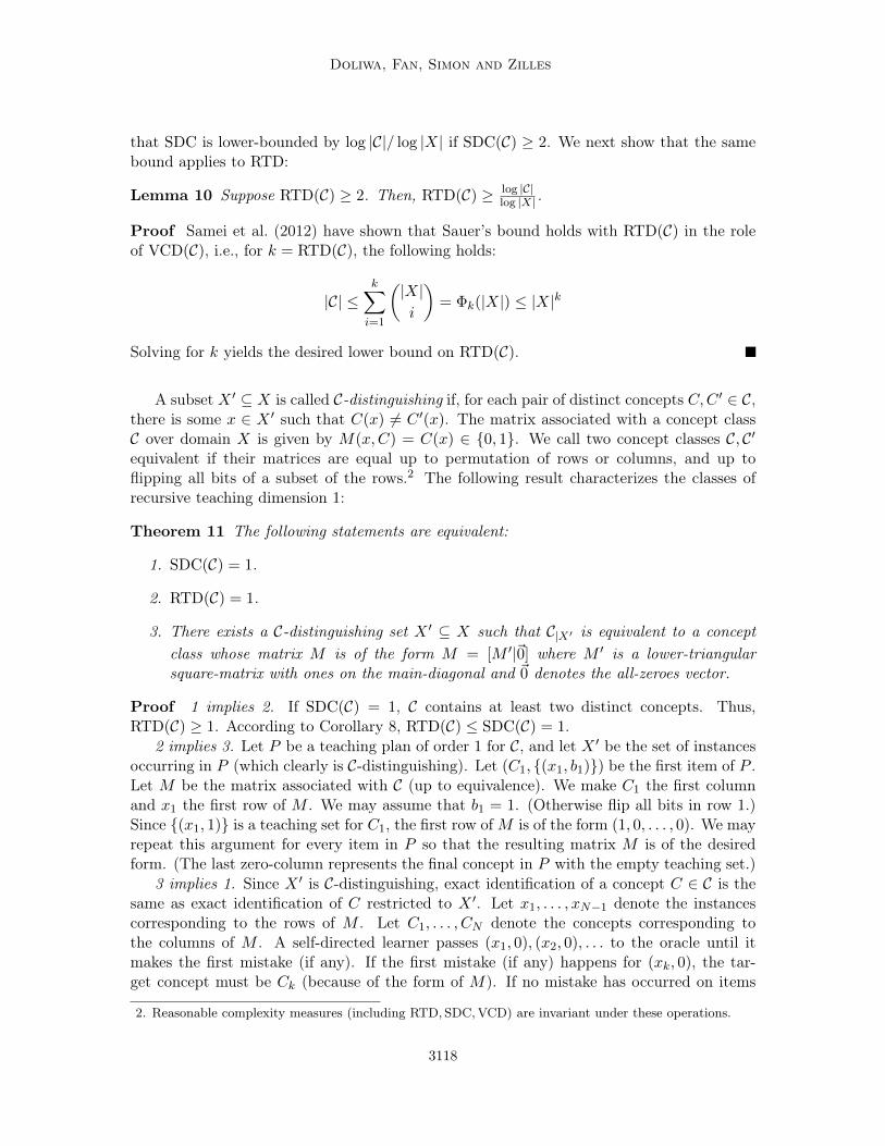
A subset X ′ ⊆ X is called C-distinguishing if, for each pair of distinct concepts C,C ′ ∈ C,there is some x ∈ X ′ such that C(x) 6= C ′(x). The matrix associated with a concept classC over domain X is given by M(x,C) = C(x) ∈ 0, 1. We call two concept classes C, C′equivalent if their matrices are equal up to permutation of rows or columns, and up toflipping all bits of a subset of the rows.2 The following result characterizes the classes ofrecursive teaching dimension 1:

Theorem 11 The following statements are equivalent:

1. SDC(C) = 1.

2. RTD(C) = 1.

3. There exists a C-distinguishing set X ′ ⊆ X such that C|X′ is equivalent to a conceptclass whose matrix M is of the form M = [M ′|~0] where M ′ is a lower-triangularsquare-matrix with ones on the main-diagonal and ~0 denotes the all-zeroes vector.

Proof 1 implies 2. If SDC(C) = 1, C contains at least two distinct concepts. Thus,RTD(C) ≥ 1. According to Corollary 8, RTD(C) ≤ SDC(C) = 1.

2 implies 3. Let P be a teaching plan of order 1 for C, and let X ′ be the set of instancesoccurring in P (which clearly is C-distinguishing). Let (C1, (x1, b1)) be the first item of P .Let M be the matrix associated with C (up to equivalence). We make C1 the first columnand x1 the first row of M . We may assume that b1 = 1. (Otherwise flip all bits in row 1.)Since (x1, 1) is a teaching set for C1, the first row of M is of the form (1, 0, . . . , 0). We mayrepeat this argument for every item in P so that the resulting matrix M is of the desiredform. (The last zero-column represents the final concept in P with the empty teaching set.)

3 implies 1. Since X ′ is C-distinguishing, exact identification of a concept C ∈ C is thesame as exact identification of C restricted to X ′. Let x1, . . . , xN−1 denote the instancescorresponding to the rows of M . Let C1, . . . , CN denote the concepts corresponding tothe columns of M . A self-directed learner passes (x1, 0), (x2, 0), . . . to the oracle until itmakes the first mistake (if any). If the first mistake (if any) happens for (xk, 0), the tar-get concept must be Ck (because of the form of M). If no mistake has occurred on items

2. Reasonable complexity measures (including RTD,SDC,VCD) are invariant under these operations.

3118


(x1, 0), . . . , (xN−1, 0), there is only one possible target concept left, namely CN . Thus theself-directed learner exactly identifies the target concept at the expense of at most one mis-take.

As we have seen in this section, the gap between SDC(C) and LC-PARTIAL(C) can bearbitrarily large (e.g., the class of half-intervals over domain [n]). We will see below, thata similar statement applies to RTD(C) and SDC(C) (despite the fact that both measuresassign value 1 to the same family of concept classes).

4. Recursive Teaching Dimension and VC-Dimension

The main open question that we pursue in this section is whether there is a universal constantk such that, for all concept classes C, RTD(C) ≤ k ·VCD(C). Clearly, TSmin(C) ≤ RTD(C) ≤RTD∗(C), so that the implications from left to right in

∀C : RTD∗(C) ≤ k ·VCD(C) ⇔ ∀C : RTD(C) ≤ k ·VCD(C)⇔ ∀C : TSmin(C) ≤ k ·VCD(C) (6)

are obvious. But the implications from right to left hold as well as can be seen from thefollowing calculations based on the assumption that TSmin(·) ≤ k ·VCD(·):

RTD∗(C) = maxX′⊆X

maxC′⊆C

TSmin(C′|X′) ≤ k · maxX′⊆X

maxC′⊆C

VCD(C′|X′) ≤ k ·VCD(C)

Here, the first equation expands the definition of RTD∗ and applies Lemma 4. The finalinequality makes use of the fact that VCD is twofold monotonic. As a consequence, thequestion of whether RTD(·) ≤ k · VCD(·) for a universal constant k remains equivalent ifRTD is replaced by TSmin or RTD∗.

4.1 Classes with RTD Exceeding VCD

In general the recursive teaching dimension can exceed the VC-dimension. Kuhlmann(1999) presents a family (Cm)m≥1 of concept classes for which VCD(Cm) = 2m but RTD(Cm)≥ TSmin(Cm) = 3m. The smallest class in Kuhlmann’s family, C1, consists of 24 conceptsover a domain of size 16.

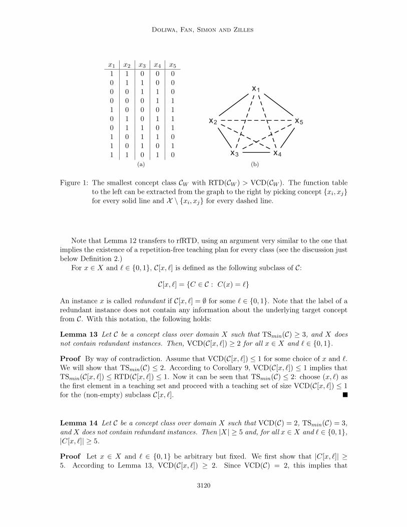
A smaller class CW with RTD(CW ) = TSmin(CW ) = 3 and VCD(CW ) = 2 was commu-nicated to us by Manfred Warmuth. It is shown in Figure 1.

Brute-force enumeration shows that RTD(CW ) = TSmin(CW ) = 3 and VCD(CW ) = 2.Warmuth’s class CW is remarkable in the sense that it is the smallest concept class for whichRTD exceeds VCD. In order to prove this, the following lemmas will be helpful.

Lemma 12 RTD(C) ≤ |X| − 1 unless C = 2X .

Proof If C 6= 2X , then C must contain a concept C such that C4x /∈ C for some instancex ∈ X. Then, C can be uniquely identified within C using the instances from X \ x andthe corresponding labels. Iterative application of this argument leads to a teaching plan forC of order at most |X| − 1.

3119


x1 x2 x3 x4 x51 1 0 0 00 1 1 0 00 0 1 1 00 0 0 1 11 0 0 0 10 1 0 1 10 1 1 0 11 0 1 1 01 0 1 0 11 1 0 1 0

(a)

x1

x2 x5

x3 x4

(b)

Figure 1: The smallest concept class CW with RTD(CW ) > VCD(CW ). The function tableto the left can be extracted from the graph to the right by picking concept xi, xjfor every solid line and X \ xi, xj for every dashed line.

Note that Lemma 12 transfers to rfRTD, using an argument very similar to the one thatimplies the existence of a repetition-free teaching plan for every class (see the discussion justbelow Definition 2.)

For x ∈ X and ` ∈ 0, 1, C[x, `] is defined as the following subclass of C:

C[x, `] = C ∈ C : C(x) = `

An instance x is called redundant if C[x, `] = ∅ for some ` ∈ 0, 1. Note that the label of aredundant instance does not contain any information about the underlying target conceptfrom C. With this notation, the following holds:

Lemma 13 Let C be a concept class over domain X such that TSmin(C) ≥ 3, and X doesnot contain redundant instances. Then, VCD(C[x, `]) ≥ 2 for all x ∈ X and ` ∈ 0, 1.

Proof By way of contradiction. Assume that VCD(C[x, `]) ≤ 1 for some choice of x and `.We will show that TSmin(C) ≤ 2. According to Corollary 9, VCD(C[x, `]) ≤ 1 implies thatTSmin(C[x, `]) ≤ RTD(C[x, `]) ≤ 1. Now it can be seen that TSmin(C) ≤ 2: choose (x, `) asthe first element in a teaching set and proceed with a teaching set of size VCD(C[x, `]) ≤ 1for the (non-empty) subclass C[x, `].

Lemma 14 Let C be a concept class over domain X such that VCD(C) = 2, TSmin(C) = 3,and X does not contain redundant instances. Then |X| ≥ 5 and, for all x ∈ X and ` ∈ 0, 1,|C[x, `]| ≥ 5.

Proof Let x ∈ X and ` ∈ 0, 1 be arbitrary but fixed. We first show that |C[x, `]| ≥5. According to Lemma 13, VCD(C[x, `]) ≥ 2. Since VCD(C) = 2, this implies that

3120


VCD(C[x, `]) = 2. Let C1, C2, C3, C4 ∈ C[x, `] be concepts that shatter two points x′, x′′

in X \ x. For at least one of these four concepts, say for C1, the neighboring conceptC14x does not belong to C (because otherwise the VC-dimension of C would be at least3). If C1, . . . , C4 were the only concepts in C[x, `], then (x′, C1(x

′)) and (x′′, C1(x′′)) would

form a teaching set for C1 in contradiction to TSmin(C) = 3. We conclude that C1, C2, C3, C4

are not the only concepts in C[x, `] so that |C[x, `]| ≥ 5.We still have to show that |X| ≥ 5. Clearly, |X| ≥ TSmin(C) = 3. Let us assume by way

of contradiction that |X| = 4, say X = x, y, z, u. We write concepts over X as 4-tuples(C(x), C(y), C(z), C(u)). The following considerations are illustrated in Figure 2. FromLemma 13 and from the assumption VCD(C) = 2, we may conclude that VCD(C[u, 0]) =2 = VCD(C[u, 1]). The set of size 2 shattered by C[u, 0] cannot coincide with the set ofsize 2 shattered by C[u, 1] because, otherwise, the VC-dimension of C would be at least 3.Let’s say, C[u, 0] shatters x, y but not x, z and C[u, 1] shatters x, z but not x, y. Bysymmetry, we may assume that C[u, 1] does not contain a concept that assigns label 1 toboth x and y, i.e., the concepts (1, 1, 0, 1) and (1, 1, 1, 1) are missing in C[u, 1]. Since x, z isshattered, C[u, 1] must contain the concepts (1, 0, 0, 1) and (1, 0, 1, 1) so as to realize the labelassignments (1, 0), (1, 1) for (x, z). Recall from the first part of the proof that |C[u, `]| ≥ 5for ` = 0, 1. Note that |C[u, `]| = 6 would imply that y, z is also shattered by C[u, `].Since VCD(C) = 2, this cannot occur for both subclasses C[u, 1] and C[u, 0] simultaneously.By symmetry, we may assume that |C[u, 1]| = 5. Thus, besides (1, 1, 0, 1) and (1, 1, 1, 1),exactly one more concept is missing in C[u, 1]. We proceed by case analysis:

Case 1: The additional missing concept in C[u, 1], say C ′, has Hamming-distance 1 fromone of (1, 1, 0, 1) and (1, 1, 1, 1). For reasons of symmetry, we may assume that C ′ =(0, 1, 1, 1). It follows that the concept (0, 1, 0, 1) belongs to C[u, 1] and has the teachingset (u, 1), (y, 1). This is a contradiction to TSmin(C) = 3.

Case 2: The additional missing concept in C[u, 1] has Hamming-distance 2 from both of(1, 1, 0, 1) and (1, 1, 1, 1). Then C[u, 1] contains (0, 1, 1, 1), (0, 1, 0, 1), (1, 0, 1, 1), and(1, 0, 0, 1). In particular, C[u, 1] shatters y, z. In this case, it cannot happen thaty, z is shattered by C[u, 0] too. Thus, |C[u, 0]| = 5. We may now expose C[u, 0] tothe same case analysis that we already applied to C[u, 1]. Since C[u, 0] does not shattery, z, Case 2 is excluded. As described above, Case 1 leads to a contradiction.

We are now ready to prove the minimality of Warmuth’s class:

Theorem 15 Let C be a concept class over domain X such that RTD(C) > VCD(C). Then|C| ≥ 10 and |X| ≥ 5.

Proof Obviously VCD(C) = 0 implies that RTD(C) = 0. According to Corollary 9,VCD(C) = 1 implies that RTD(C) = 1. So we may safely assume that VCD(C) ≥ 2 andRTD(C) ≥ 3. According to Lemma 4, we may assume that RTD(C) = TSmin(C) because,otherwise, our proof could proceed with the class C′ ⊆ C such that RTD(C′) = TSmin(C′).We may furthermore assume that C[x, `] 6= ∅ for all x ∈ X and ` ∈ 0, 1 because, otherwise,x is a redundant instance and the proof could proceed with the subdomain X \x. We may

3121


0011

0001

1101

0111 1111

0101

1011

1001

z

y

x

u = 0x,y shattered

u = 1x,z shattered

Figure 2: As indicated by circles, the concepts 1101 and 1111 are missing in C[u, 1].There is exactly one additional concept C ′ which is missing. If C ′ ∈0101, 0111, 1001, 1011, then C ′ has a teaching set of size 2. Otherwise, C[u, 1]shatters y, z.

therefore apply Lemma 13 and conclude that VCD(C[x, `]) ≥ 2 for all x ∈ X and ` ∈ 0, 1.Clearly |X| ≥ RTD(C) ≥ 3. We claim that |X| ≥ 5, which can be seen as follows. First,note that C 6= 2X , because RTD(C) > VCD(C). Thus RTD(C) ≤ |X| − 1 by Lemma 12so that |X| ≥ RTD(C) + 1 ≥ 4. Assume |X| = 4 by way of contradiction. It follows thatRTD(C) ≤ 3 and VCD(C) ≤ 2. Thus, RTD(C) = 3 and VCD(C) = 2. But then |X| ≥ 5 byLemma 14. Having established |X| ≥ 5, it remains to prove that |C| ≥ 10. According to (1),RTD(C) ≤ log |C|. RTD(C) ≥ 4 would imply that |C| ≥ 16 > 10. We may therefore focuson the case RTD(C) = 3, which implies that VCD(C) = 2. But now it is immediate fromLemma 14 that |C| ≥ 10, as desired.

We close this section by showing that RTD(C)− VCD(C) can become arbitrarily large.This can be shown by a class whose concepts are disjoint unions of concepts taken fromWarmuth’s class CW . Details follow. Suppose that C1 and C2 are concept classes overdomains X1 and X2, respectively, such that X1 ∩X2 = ∅. Then

C1 ] C2 := A ∪B| A ∈ C1, B ∈ C2 .

We apply the same operation to arbitrary pairs of concept classes with the understandingthat, after renaming instances if necessary, the underlying domains are disjoint. We claimthat VCD, TSmin and RTD behave additively with respect to “]”, i.e., the following holds:

Lemma 16 For all K ∈ VCD,TSmin,RTD: K(C1 ] C2) = K(C1) + K(C2).

Proof The lemma is fairly obvious for K = VCD and K = TSmin. Suppose that wehave an optimal teaching plan that teaches the concepts from C1 in the order A1, . . . , AM

(resp. the concepts from C2 in the order B1, . . . , BN ). Then, the teaching plan that proceedsin rounds and teaches Ai∪B1, . . . , Ai∪BN in round i ∈ [M ] witnesses that RTD(C1]C2) ≤

3122


RTD(C1) + RTD(C2). The reverse direction is an easy application of Lemma 4. ChooseC′1 ⊆ C1 and C′2 ⊆ C2 so that RTD(C1) = TSmin(C′1) and RTD(C2) = TSmin(C′2). Now itfollows that

RTD(C1 ] C2) ≥ TSmin(C′1 ] C′2) = TSmin(C′1) + TSmin(C′2) = RTD(C1) + RTD(C2) .

Setting CnW = CW ] . . . ] CW with n duplicates of CW on the right-hand side, we nowobtain the following result as an immediate application of Lemma 16:

Theorem 17 VCD(CnW ) = 2n and RTD(CnW ) = 3n.

We remark here that the same kind of reasoning cannot be applied to blow up rfRTD,because rfRTD(C]C) can in general be smaller than 2·rfRTD(C): considering again the classC with rfRTD(C) = 3 from Table 1, simple brute-force computations show that rfRTD(C ×C) = 5.

4.2 Intersection-closed Classes

As shown by Kuhlmann (1999), TSmin(C) ≤ I(C) holds for every intersection-closed conceptclass C. Kuhlmann’s central argument (which occurred first in a proof of a related resultby Goldman and Sloan (1994)) can be applied recursively so that the following is obtained:

Lemma 18 For every intersection-closed class C, RTD(C) ≤ I(C).

Proof Let k := I(C). We present a teaching plan for C of order at most k. Let C1, . . . , CN

be the concepts in C in topological order such that Ci ⊃ Cj implies i < j. It follows that,for every i ∈ [N ], Ci is an inclusion-maximal concept in Ci := Ci, . . . , CN. Let Si denotea minimal spanning set for Ci w.r.t. C. Then:

• |Si| ≤ k and Ci is the unique minimal concept in C that contains Si.

• As Ci is inclusion-maximal in Ci, Ci is the only concept in Ci that contains Si.

Thus (x, 1) | x ∈ Si is a teaching set of size at most k for Ci in Ci.

Since I(C) ≤ VCD(C), we get

Corollary 19 For every intersection-closed class C, RTD(C) ≤ VCD(C).

This implies RTD∗(C) ≤ VCD(C) for every intersection-closed class C, since the property“intersection-closed” is preserved when reducing a class C to C|X′ for X ′ ⊆ X.

For every fixed constant d (e.g., d = 2), Kuhlmann (1999) presents a family (Cm)m≥1 ofintersection-closed concept classes such that the following holds:3

∀m ≥ 1 : VCD(Cm) = d and SDC(Cm) ≥ m. (7)

3. A family satisfying (7) but not being intersection-closed was presented previously by Ben-David andEiron (1998).

3123


This shows that SDC(C) can in general not be upper-bounded by I(C) or VCD(C). It showsfurthermore that the gap between RTD(C) and SDC(C) can be arbitrarily large (even forintersection-closed classes).

Lemma 18 generalizes to nested differences:

Theorem 20 If C is intersection-closed then RTD(DIFF≤d(C)) ≤ d · I(C).

Proof Any concept C ∈ DIFF≤d(C) can be written in the form

C = C1 \=:D1︷︸︸︷

(C2 \ (· · · (Cd−1 \ Cd) · · · )) (8)

such that, for every j, Cj ∈ C ∪ ∅, Cj ⊇ Cj+1, and this inclusion is proper unless Cj =∅. Let Dj = Cj+1 \ (Cj+2 \ (· · · (Cd−1 \ Cd) · · · )). We may obviously assume that therepresentation (8) of C is minimal in the following sense:

∀j = 1, . . . , d : Cj = 〈Cj \Dj〉C (9)

We define a lexicographic ordering, A, on concepts from DIFF≤d(C) as follows. Let C be aconcept with a minimal representation of the form (8), and let the minimal representationof C ′ be given similarly in terms of C ′j , D

′j . Then, by definition, C A C ′ if C1 ⊃ C ′1 or

C1 = C ′1 ∧D1 A D′1.Let k := I(C). We present a teaching plan of order at most dk for DIFF≤d(C). Therein,

the concepts are in lexicographic order so that, when teaching concept C with minimal rep-resentation (8), the concepts preceding C w.r.t. A have been discarded already. A teachingset T for C is then obtained as follows:

• For every j = 1, . . . , d, include in T a minimal spanning set for Cj \ Dj w.r.t. C.Augment its instances by label 1 if j is odd, and by label 0 otherwise.

By construction, C as given by (8) and (9) is the lexicographically smallest concept inDIFF≤d(C) that is consistent with T . Since concepts being lexicographically larger than Chave been discarded already, T is a teaching set for C.

Corollary 21 Let C1, . . . , Cr be intersection-closed classes over the domain X. Assume thatthe “universal concept” X belongs to each of these classes.4 Then,

RTD(

DIFF≤d(C1 ∪ · · · ∪ Cr))≤ d ·

r∑i=1

I(Ci) .

Proof Consider the concept class C := C1∧· · ·∧Cr := C1∩· · ·∩Cr | Ci ∈ Ci for i = 1, . . . , r.According to Helmbold et al. (1990), we have:

1. C1 ∪ · · · ∪ Cr is a subclass of C.

4. This assumption is not restrictive: adding the universal concept to an intersection-closed class does notdestroy the property of being intersection-closed.

3124


2. C is intersection-closed.

3. Let C = C1 ∩ · · · ∩ Cr ∈ C. For all i, let Si be a spanning set for C w.r.t. Ci, i.e.,Si ⊆ C and 〈Si〉Ci = 〈C〉Ci . Then S1 ∪ · · · ∪ Sr is a spanning set for C w.r.t. C.

Thus I(C) ≤ I(C1) + · · ·+ I(Cr). The corollary follows from Theorem 20.

4.3 Maximum Classes

In this section, we show that the recursive teaching dimension coincides with the VC-dimension on the family of maximum classes. In a maximum class C, every set of k ≤ VCD(C)instances is shattered, which implies RTD(C) ≥ TSmin(C) ≥ VCD(C). Thus, we can focuson the reverse direction and pursue the question whether RTD(C) ≤ VCD(C). We shall an-swer this question in the affirmative by establishing a connection between “teaching plans”and “corner-peeling plans”.

We say that a corner-peeling plan (5) is strong if Condition 2 in Definition 6 is replacedas follows:

2’. For all t = 1, . . . , N , C′t is a cube in Ct, . . . , CN which contains Ct and whose colors(augmented by their labels according to Ct) form a teaching set for Ct ∈ Ct, . . . , CN.

We denote the set of colors of C′t as Xt and its augmentation by labels according to Ct asSt in what follows. The following result is obvious:

Lemma 22 A strong corner-peeling plan of the form (5) induces a teaching plan of theform (2) of the same order.

The following result justifies the attribute “strong” of corner-peeling plans:

Lemma 23 Every strong corner-peeling plan is a corner-peeling plan.

Proof Assume that Condition 2 is violated. Then there is a color x ∈ X \Xt and a conceptC ∈ Ct+1, . . . , CN such that C coincides with Ct on all instances except x. But then C isconsistent with set St so that St is not a teaching set for Ct ∈ Ct, . . . , CN, and Condition2’ is violated as well.

Lemma 24 Let C be a shortest-path closed concept class. Then, every corner-peeling planfor C is strong.

Proof Assume that Condition 2’ is violated. Then some C ∈ Ct+1, . . . , CN is consistentwith St. Thus, the shortest path between C and Ct in G(Ct, . . . , CN) does not enter thecube C′t. Hence there is a concept C ′ ∈ Ct+1, . . . , CN \ C′t that is a neighbor of Ct inG(Ct, . . . , CN), and Condition 2 is violated.

As maximum classes are shortest-path closed (Kuzmin and Warmuth, 2007), we obtain:

3125


Corollary 25 Every corner-peeling plan for a maximum class is strong, and therefore in-duces a teaching plan of the same order.

Since Rubinstein and Rubinstein (2012) showed that every maximum class C can beVCD(C)-corner-peeled, we may conclude that RTD(C) ≤ VCD(C). As mentioned above,RTD(C) ≥ TSmin(C) ≥ VCD(C) for every maximum class C. Thus the following holds:

Theorem 26 For every maximum class C, RTD(C) = TSmin(C) = VCD(C).

The fact that, for every maximum class C and every X ′ ⊆ X, the class C|X′ is stillmaximum implies that RTD∗(C) = VCD(C) for every maximum class C.

We establish a connection between repetition-free teaching plans and representationshaving the acyclic non-clashing property:

Lemma 27 Let C be an arbitrary concept class. Then the following holds:

1. Every repetition-free teaching plan (2) of order d for C induces a representation map-ping r of order d for C given by r(Ct) = X(St) for t = 1, . . . , N . Moreover, r has theacyclic non-clashing property.

2. Every representation mapping r of order d for C that has the acyclic non-clashingproperty (4) induces a teaching plan (2) given by St = (x,Ct(x)) | x ∈ r(Ct) fort = 1, . . . , N . Moreover, this plan is repetition-free.

Proof

1. A clash between Ct and Ct′ , t < t′, on X(St) would contradict the fact that St is ateaching set for Ct ∈ Ct, . . . , CN.

2. Conversely, if St = (x,Ct(x)) | x ∈ r(Ct) is not a teaching set for Ct ∈ Ct, . . . , CN,then there must be a clash on X(St) between Ct and a concept from Ct+1, . . . , CN.The teaching plan induced by r is obviously repetition-free since r is injective.

Corollary 28 Let C be maximum of VC-dimension d. Then, there is a one-one mappingbetween repetition-free teaching plans of order d for C and unlabeled compression schemeswith the acyclic non-clashing property.

A closer look at the work by Rubinstein and Rubinstein (2012) reveals that corner-peeling leads to an unlabeled compression scheme with the acyclic non-clashing property(again implying that RTD(C) ≤ VCD(C) for maximum classes C). Similarly, an inspectionof the work by Kuzmin and Warmuth (2007) reveals that the unlabeled compression schemeobtained by the Tail Matching Algorithm has the acyclic non-clashing property, too. Thus,this algorithm too can be used to generate a recursive teaching plan of order VCD(C) forany maximum class C.

It is not known to date whether every concept class C of VC-dimension d can be embed-ded into a maximum concept class C′ ⊇ C of VC-dimension O(d). Indeed, finding such an

3126


embedding is considered as a promising method for settling the sample compression conjec-ture. It is easy to see that a negative answer to our question "Is RTD(C) ∈ O(VCD(C))?"would deem this approach fruitless:

Theorem 29 If RTD(C) is not linearly bounded in VCD(C), then there is no mappingC 7→ C′ ⊇ C such that C′ is maximum and VCD(C′) is linearly bounded in VCD(C).

Proof Suppose there is a universal constant k and a mapping MAXIMIZE that maps everyconcept class C to a concept class C′ ⊇ C such that C′ is maximum and VCD(C′) ≤ k·VCD(C).It follows that, for any concept class C, the following holds:

RTD(C) ≤ RTD(MAXIMIZE(C)) = VCD(MAXIMIZE(C)) ≤ k ·VCD(C))

where the equation RTD(MAXIMIZE(C)) = VCD(MAXIMIZE(C)) follows from Theo-rem 26.

According to (6), this theorem still holds if RTD is replaced by RTD∗.

4.4 Shortest-Path Closed Classes

In this section, we study the best-case teaching dimension, TSmin(C), and the average-caseteaching-dimension, TSavg(C), of a shortest-path closed concept class C.

It is known that the instances of I(C;G(C)), augmented by their C-labels, form a uniqueminimal teaching set for C in C provided that C is a maximum class (Kuzmin and Warmuth,2007). Lemma 30 slightly generalizes this observation.

Lemma 30 Let C be any concept class. Then the following two statements are equivalent:

1. C is shortest-path closed.

2. Every C ∈ C has a unique minimum teaching set S, namely the set S such thatX(S) = I(C;G(C)).

Proof 1 ⇒ 2 is easy to see. Let C be shortest-path closed, and let C be any concept inC. Clearly, any teaching set S for C must satisfy I(C;G(C)) ⊆ X(S) because C must bedistinguished from all its neighbors in G(C). Let C ′ 6= C be any other concept in C. SinceC and C ′ are connected by a path P of length |C 4 C ′|, C and C ′ are distinguished bythe color of the first edge in P , say by the color x ∈ I(C;G(C)). Thus, no other instances(=colors) besides I(C;G(C)) are needed to distinguish C from any other concept in C.

To show 2 ⇒ 1, we suppose 2 and prove by induction on k that any two conceptsC,C ′ ∈ C with k = |C4C ′| are connected by a path of length k in G(C). The case k = 1 istrivial. For a fixed k, assume all pairs of concepts of Hamming distance k are connected by apath of length k in G(C). Let C,C ′ ∈ C with |C4C ′| = k+1 ≥ 2. Since I(C;G(C)) = X(S),there is an x ∈ I(C;G(C)) such that C(x) 6= C ′(x). Let C ′′ be the x-neighbor of C in G(C).Note that C ′′(x) = C ′(x) so that C ′′ and C ′ have Hamming-distance k. According to theinductive hypothesis, there is a path of length k from C ′′ to C ′ in G(C). It follows that Cand C ′ are connected by a path of length k + 1.

3127


Theorem 31 Let C be a shortest-path closed concept class. Then, TSavg(C) < 2VCD(C).

Proof According to Lemma 30, the average-case teaching dimension of C coincides withthe average vertex-degree in G(C), which is twice the density of G(C). As mentioned inSection 2.4 already, dens(G(C)) < VCD(C).

Theorem 31 generalizes a result by Kuhlmann (1999) who showed that the average-caseteaching dimension of “d-balls” (sets of concepts of Hamming distance at most d from acenter concept) is smaller than 2d. It also simplifies Kuhlmann’s proof substantially. InTheorem 4 of the same paper, Kuhlmann (1999) stated furthermore that TSavg(C) < 2 ifVCD(C) = 1, but his proof is flawed.5 Despite the flawed proof, the claim itself is correctas we show now:

Theorem 32 Let C be any concept class. If VCD(C) = 1 then TSavg(C) < 2.

Proof By Theorem 31, the average-case teaching dimension of a maximum class of VC-dimension 1 is less than 2. It thus suffices to show that any class C of VC-dimension 1 can betransformed into a maximum class C′ of VC-dimension 1 without decreasing the average-caseteaching dimension. Let X ′ ⊆ X be a minimal set that is C-distinguishing, i.e., for every pairof distinct concepts C,C ′ ∈ C, there is some x ∈ X ′ such that C(x) 6= C(x′). Let m = |X|and C′ = C|X′ . Obviously, |C′| = |C| and VCD(C′) = 1 so that |C′| ≤

(m0

)+(m1

)= m + 1.

Now we prove that C′ is maximum. Note that every x ∈ X ′ occurs as a color in G(C′)because, otherwise, X ′ \ x would still be C-distinguishing (which would contradict theminimality of X ′). As VCD(C′) = 1, no color can occur twice. Thus |E(G(C′))| = m.Moreover, there is no cycle in G(C′) since a cycle would require at least one repeated color.As G(C′) is an acyclic graph of m edges, it has at least m + 1 vertices, i.e. |C′| ≥ m + 1.Thus, |C′| = m + 1 and C′ is maximum. This implies that TSavg(C′) < 2VCD(C′). SinceX ′ ⊆ X but X ′ is still C-distinguishing, we obtain TS(C; C) ≤ TS(C|X′ , C′) for all C ∈ C.Thus, TSavg(C) ≤ TSavg(C′) < 2VCD(C′) = 2, which concludes the proof.

We briefly note that TSavg(C) cannot in general be bounded by O(VCD(C)). Kushilevitzet al. (1996) present a family (Cn) of concept classes such that TSavg(Cn) = Ω(

√|Cn|) but

VCD(Cn) ≤ log |Cn|.We conclude this section by showing that there are shortest-path closed classes for which

RTD exceeds VCD.

Lemma 33 If degG(C)(C) ≥ |X| − 1 for all C ∈ C, then C is shortest-path closed.

Proof Assume by way of contradiction that C is not shortest-path closed. Pick two con-cepts C,C ′ ∈ C of minimal Hamming-distance, say d, subject to the constraint of not beingconnected by a path of length d in G(C). It follows that d ≥ 2. By the minimality of d, any

5. His Claim 2 states the following. If VCD(C) = 1, C1, C2 ∈ C, x ∈ X, x /∈ C1, C2 = C1 ∪ x,then, for either (i, j) = (1, 2) or (i, j) = (2, 1), one obtains TS(Ci; C) = TS(Ci − x; C − x) + 1 andTS(Cj ; C) = 1. This is not correct, as can be shown by the class C = xz : 1 ≤ z ≤ k : 0 ≤ k ≤ 5 overX = xk : 1 ≤ k ≤ 5, which has VC-dimension 1. For C1 = x1, x2, C2 = x1, x2, x3, and x = x3, weget TS(C1; C) = TS(C2; C) = TS(C1 − x; C − x) = 2.

3128


neighbor of C with Hamming-distance d − 1 to C ′ does not belong to C. Since there ared such missing neighbors, the degree of C in G(C) is bounded by |X| − d ≤ |X| − 2. Thisyields a contradiction.

Rubinstein et al. (2009) present a concept class C with TSmin(C) > VCD(C). An in-spection of this class shows that the minimum vertex degree in its 1-inclusion graph is|X|−1. According to Lemma 33, this class must be shortest-path closed. Thus, the inequal-ity TSmin(C) ≤ VCD(C) does not generalize from maximum classes to shortest-path closedclasses.

5. Conclusions

This paper relates the RTD, a recently introduced teaching complexity notion, to informationcomplexity parameters of various classical learning models.

One of these parameters is SDC, the information complexity of self-directed learning,which constitutes the most information-efficient query learning model known to date. Ourmain result in this context, namely lower-bounding the SDC by the RTD, has implicationsfor the analysis of information complexity in teaching and learning. In particular, everyupper bound on SDC holds for RTD; every lower bound on RTD holds for SDC.

The central parameter in our comparison is the VC-dimension. Although the VC-dimension can be arbitrarily large for classes of recursive teaching dimension 1 (which iswell-known and also evident from Theorem 11) and arbitrarily smaller than SDC (Ben-Davidand Eiron, 1998; Kuhlmann, 1999), it does not generally lie in between the two. However,while the SDC cannot be upper-bounded by any linear function of the VC-dimension, itis still open whether such a bound exists for the RTD. The existence of the latter wouldmean that the combinatorial properties that determine the information complexity of PAC-learning (i.e., of learning from randomly drawn examples) are essentially the same as thosethat determine the information complexity of teaching (i.e., of learning from helpfully se-lected examples), at least when using the recursive teaching model.

As a partial solution to this open question, we showed that the VC-dimension coincideswith the RTD in the special case of maximum classes. Our results, and in particular the re-markable correspondence to unlabeled compression schemes, suggest that the RTD is basedon a combinatorial structure that is of high relevance for the complexity of information-efficient learning and sample compression. Analyzing the circumstances under which teach-ing plans defining the RTD can be used to construct compression schemes (and to boundtheir size) seems to be a promising step towards new insights into the theory of samplecompression.

Acknowledgments

We would like to thank Manfred Warmuth for the permission to include the concept classfrom Figure 1 in this paper. Moreover, we would like to thank Malte Darnstädt and MichaelKallweit for helpful and inspiring discussions, and the anonymous referees of both this article

3129


and its earlier conference version for many helpful suggestions and for pointing out mistakesin the proofs of Theorems 20 and 32.

This work was supported by the Natural Sciences and Engineering Research Council ofCanada (NSERC).

References

Dana Angluin. Queries and concept learning. Machine Learning, 2(4):319–342, 1988.

Frank Balbach. Measuring teachability using variants of the teaching dimension. TheoreticalComputer Science, 397(1–3):94–113, 2008.

Shai Ben-David and Nadav Eiron. Self-directed learning and its relation to the VC-dimensionand to teacher-directed learning. Machine Learning, 33(1):87–104, 1998.

Anselm Blumer, Andrzej Ehrenfeucht, David Haussler, and Manfred K. Warmuth. Learn-ability and the Vapnik-Chervonenkis dimension. Journal of the Association on ComputingMachinery, 36(4):929–965, 1989.

Malte Darnstädt, Thorsten Doliwa, Hans U. Simon, and Sandra Zilles. Order compressionschemes. In Proceedings of the 24th International Conference on Algorithmic LearningTheory, pages 173–187, 2013.

Thorsten Doliwa, Hans U. Simon, and Sandra Zilles. Recursive teaching dimension, learningcomplexity, and maximum classes. In Proceedings of the 21st International Conference onAlgorithmic Learning Theory, pages 209–223, 2010.

Sally Floyd and Manfred Warmuth. Sample compression, learnability, and the Vapnik-Chervonenkis dimension. Machine Learning, 21(3):1–36, 1995.

Sally A. Goldman and Michael J. Kearns. On the complexity of teaching. Journal ofComputer and System Sciences, 50(1):20–31, 1995.

Sally A. Goldman and Robert H. Sloan. The power of self-directed learning. MachineLearning, 14(1):271–294, 1994.

Sally A. Goldman, Ronald L. Rivest, and Robert E. Schapire. Learning binary relations andtotal orders. SIAM Journal on Computing, 22(5):1006–1034, 1993.

David Haussler, Nick Littlestone, and Manfred K. Warmuth. Predicting 0, 1 functions onrandomly drawn points. Information and Computation, 115(2):284–293, 1994.

David Helmbold, Robert Sloan, and Manfred K. Warmuth. Learning nested differences ofintersection-closed concept classes. Machine Learning, 5:165–196, 1990.

Christian Kuhlmann. On teaching and learning intersection-closed concept classes. In Pro-ceedings of the 4th European Conference on Computational Learning Theory, pages 168–182, 1999.

3130


Eyal Kushilevitz, Nathan Linial, Yuri Rabinovich, and Michael E. Saks. Witness sets forfamilies of binary vectors. J. Comb. Theory, Ser. A, 73(2):376–380, 1996.

Dima Kuzmin and Manfred K. Warmuth. Unlabeled compression schemes for maximumclasses. Journal of Machine Learning Research, 8:2047–2081, 2007.

Nick Littlestone. Learning quickly when irrelevant attributes abound: a new linear thresholdalgorithm. Machine Learning, 2(4):245–318, 1988.

Nick Littlestone and Manfred K. Warmuth. Relating data compression and learnability.Technical Report, UC Santa Cruz, 1996.

Wolfgang Maass and György Turán. Lower bound methods and separation results for on-linelearning models. Machine Learning, 9:107–145, 1992.

Balas K. Natarajan. On learning boolean functions. In Proceedings of the 19th AnnualSymposium on Theory of Computing, pages 296–304, 1987.

Benjamin I. P. Rubinstein and J. Hyam Rubinstein. A geometric approach to sample com-pression. Journal of Machine Learning Research, 13:1221–1261, 2012.

Benjamin I. P. Rubinstein, Peter L. Bartlett, and J. Hyam Rubinstein. Shifting: One-inclusion mistake bounds and sample compression. Journal of Computer and SystemSciences, 75(1):37–59, 2009.

Rahim Samei, Pavel Semukhin, Boting Yang, and Sandra Zilles. Sauer’s bound for a notionof teaching complexity. In Proceedings of the 23rd International Conference on AlgorithmicLearning Theory, pages 96–110, 2012.

Norbert Sauer. On the density of families of sets. Journal of Combinatorial Theory, SeriesA, 13(1):145–147, 1972.

Ayumi Shinohara and Satoru Miyano. Teachability in computational learning. New Gener-ation Computing, 8(4):337–348, 1991.

Leslie G. Valiant. A theory of the learnable. Communications of the ACM, 27(11):1134–1142,1984.

Vladimir N. Vapnik and Alexey Ya. Chervonenkis. On the uniform convergence of relativefrequencies of events to their probabilities. Theor. Probability and Appl., 16(2):264–280,1971.

Emo Welzl. Complete range spaces, 1987. Unpublished Notes.

Sandra Zilles, Steffen Lange, Robert Holte, and Martin Zinkevich. Teaching dimensionsbased on cooperative learning. In Proceedings of the 21st Annual Conference on LearningTheory, pages 135–146, 2008.

Sandra Zilles, Steffen Lange, Robert Holte, and Martin Zinkevich. Models of cooperativeteaching and learning. Journal of Machine Learning Research, 12:349–384, 2011.

3131

recursive teaching dimension, vc-dimension and sample...

Documents