Available online at www.sciencedirect.com

08) 653–663

Intelligence 36 (20

Recruitment modeling: An analysis and an application to the study ofmale–female differences in intelligence☆

Earl Hunt ⁎, Tara Madhyastha

The University of Washington

Received 1 December 2006; received in revised form 26 February 2008; accepted 20 March 2008Available online 16 May 2008

Abstract

Studies of group differences in intelligence often invite conclusions about groups in general from studies of group differences inselected populations. The same design is used in the study of group differences in other traits as well. Investigators observe samplesfrom two groups (e.g. men and women) in some accessible population, but seek to conclude something about a wider, generalpopulation. The most frequent case is probably a study contrasting undergraduate men and women. The investigator will know themethod by which people are recruited from the accessible population. However the methods by which the members of each groupenter the accessible population from the general population is not under the control of the investigator. Call this the recruitmentprocess. The recruitment process may introduce differences between groups in the accessible population that do not occur in thegeneral population. Continuing the example, the recruitment processes that draw men and women from the college-age populationinto the population of students may not be the same. Therefore, in order to draw an inference about group differences in the generalpopulation from group differences in samples from the accessible population it is necessary to have a model of the recruitmentprocess. We develop such a model, and present data showing that it appears to be valid for the case of recruitment into thepopulation of youth who consider post-secondary education. We illustrate use of the model by analyzing findings from a widelypublicized study of differences in intelligence between men and women, and show that the conclusions from that study aremodified by consideration of the recruitment process.© 2008 Elsevier Inc. All rights reserved.

Keywords: Intelligence; Male–female differences; Sampling; Population estimates; Gender differences; Mathematical modeling

1. Introduction

Many studies of intelligence, and indeed, many studiesin psychology in general, use the following paradigm. Theresearcher wishes to draw an inference about differencesbetween two or more groups along some trait (here

☆ We thank Paul Irwing and Wendy Johnson for helpful,constructive comments on earlier drafts of this paper.⁎ Corresponding author. Department of Psychology Box 351525,

University of Washington, Seattle, WA 98195-1525, United States.E-mail address: ehunt@u.washington.edu (E. Hunt).

0160-2896/$ - see front matter © 2008 Elsevier Inc. All rights reserved.doi:10.1016/j.intell.2008.03.002

intelligence). Because it is often infeasible to construct atrue random sample of the general population, theresearcher observes the difference in a sample fromsome population that can readily be tested (e.g., collegestudents,military personnel, or public school students).Wewill refer to this as the accessible population. The problemis that recruitment from the general population to theaccessible population may be different for each groupwithin the overall population. To take an obvious case,compared to their frequencies in the general population,men are overrepresented and women are underrepresentedin the United States Armed Services. It is highly likely that

1 We accept Jackson and Rushton's statement. We have been unableto reanalyze their data directly as the College Board does not have thisdata in their current archives. According to Rushton (personalcommunication, April 8, 2007) Jackson, who is now deceased, hadphysical custody of the data and it is no longer available.

654 E. Hunt, T. Madhyastha / Intelligence 36 (2008) 653–663

the psychological factors that influence aman's decision toenlist are not the same as those that influence a woman toenlist. It would be inappropriate to draw an unqualifiedconclusion about a psychological difference between menand women based upon observations of differencesbetween service men and women. More abstractly, whenthere are inter-group differences in recruitment from thegeneral to the accessible population, it is inappropriate togeneralize results about group differences observed in thesample to the general population, even if the sample is arandom sample of the accessible population.

Once stated, the problem is obvious. But what can wedo about it? In this paper we approach the problem byconstructing mathematical models of the process bywhich members of different groups are recruited fromthe general population to the accessible population. Wewill refer to them as recruitment models. These modelscan be used to generalize results based upon a sample ofthe accessible population to form a conclusion about thegeneral population.

Wewill illustrate our methods by considering amuch-studied, much debated topic: differences in intelligencebetween men and women. More particularly, we willexamine a highly publicized recent finding claiming thatthere are such differences, in favor of men, and will showthat when recruitment effects are considered theconclusion of the original authors must be substantiallymodified. We regard this finding as interesting in itself.However we believe that in the long run the methodol-ogy behind our reasoning is likely to be of moreimportance than the specific finding, because it providesa potential solution to the recruitment problem.

We will first describe the example. We then considerbriefly a simple recruitment model that has beenpreviously applied to the study of group differences inintelligence. The reason for doing so is because thismodelhas been used before. We then consider a more realisticrecruitment model, provide data showing its validity, andthen apply it to the example.

2. The example

Jackson and Rushton (2006) claimed that there isapproximately a 4 IQ point (.24 SD units) male–femaledifference in general intelligence, in favor of males. Theybased this conclusion on an analysis of approximately100,000 examinees in the Scholastic Assessment Test(SAT) validation study sample of 1991. Jackson andRushton extracted a general factor from individual itemscores on the math and verbal subsections of the SAT, andthen compared the scores of men and women on thatgeneral factor. They also found that there was a higher

percentage of men than women in all score ranges abovethe mean, and a higher percentage of women than men inranges below the mean. Jackson and Rushton argued thatthis rules out the possibility that male scores are higherbecause males have higher variability in intelligence (e.g.Jensen, 1998, pg. 537), on the grounds that they did notobserve an excess of males in both the high and lowscoring categories of the SAT. They included in theirpaper the caution that it would be interesting to see if thisfinding could be repeated in a more general population.

Their paper generated a good deal of attention in thepopular press. Rushton was interviewed on television.Jackson and Rushton's conclusion was also mentioned,usually with skepticism, in a number of editorials in thepopular press. To the best of our knowledge, none ofthese interviews or commentaries questioned whetherthe validity study sample was representative of thegeneral population, or included the original authors'caution that the finding should be repeated in a moregeneral population.

There is reason to believe that Jackson and Rushton'sstudy was influenced by substantial recruitment effects.The accessible population, students who take the SAT ina given year, is constructed by self selection from thegeneral population of students in their last two years ofhigh school. In Jackson and Rushton's data set, whichwe assume was an appropriate sample of the accessiblepopulation, approximately 55% of the examinees werewomen. However, according to the US census approxi-mately 49% of people aged 15–19 are female. Thissuggests that for some reason women are more likely tochoose to take the SAT than are men.

We shall show, by applying recruitment models, thatthe Jackson and Rushton results could be produced evenif the mean intelligence of women was equal to the meanintelligence of men in the general population.

3. The recruitment issue illustrated by the Jacksonand Rushton dataset

Jackson and Rushton examined a 1991 validity studysample of the Scholastic Assessment Test (SAT). This setcontained scores for 46,509 men and 56,007 women.They describe the sample by saying “about 50% of theUS population now go to college and SAT test takers arerepresentative of those who aspire to do so.” (Jackson &Rushton , 2006, pg. 480). 1 The re is a dispa rity between

655E. Hunt, T. Madhyastha / Intelligence 36 (2008) 653–663

ratio of men to women in Jackson and Rushton's sampleand in the population. The ratio in the sample was .83.According to the US census data for 1990, the ratio ofmen to women in the United States was 1.04:1, i.e.slightly more men than women. In addition, a higherpercentage of women than men complete high school.Estimates of dropout rates vary significantly dependingon how they are calculated.2 However, a recent study( Losen, Orfiel d, Wald, & Swanson, 2004) has esti mateddropout rates at the turn of the century to be 32%. TheNational Center for Education Statistics (2006) hasestimated the 1991–1992 graduation rate to have been73.2% of the population of 17 year olds. Currently, thereis an 8% difference in dropout rates between men (36%)and women (28%). This is somewhat controversial, sowe will assume that men and women both drop out at the32% rate. (Were we to use differential dropout rates theeffects we shall describe would increase.) Finally, in thehigh school population, more females than males takethe SAT. In 1991–1992, 52.45% of SAT test takers werewomen, and that percentage has been increasing. This isclose to the percentage in Jackson and Rushton's sample.

A two stage recruitment process applied; recruitmentinto the class of high school juniors and seniors, and theninto the subset of the class who decide to take the SAT.The recruitment process was in all likelihood related towhatever trait causes people to have high SATscores, fora massive literature has shown that people with high testscores are less likely to drop out of high school and morelikely to enter college than people with low test scores.Jackson and Rushton refer to this trait as intelligence (g),and we shall follow their lead. Because the recruitmentprocess has been more selective for men than women,and has selected against low intelligence, it is virtuallycertain that an estimate of the differences between maleand female test scores in the (differentially recruited)sample will be biased toward overestimating thedifference in intelligence between men and women inthe population. But what is the extent of the bias?

4. The left censored model

Faced with an analogous problem in another article inthis journal, estimation of differences in intelligencescores across states in the United States from SATscores, Kanazawa (2006) applied a recruitment modelthat he referred to as the left censored model. He

2 A related statistic, the percentage of the population age 16–24 whoare not high school graduates has varied between 12.5% and 9.4% ,with most figures close to 11%. A very small time trend is discernible(National Center for Educational Statistics, 2006, Table 104).

assumed that anyone who completes high school would,if tested, have had a higher test score than everyone whodoes not, and that anyone who takes the SAT wouldhave a higher test score than everyone who does not. Asthe name implies, the left censored model amounts toobserving the distribution of scores above a certainknown percentile, and estimating the distribution of allscores from these observations.

We now apply the left censored model to calculatethe expected mean differences in Jackson and Rushton'ssample, assuming that there is no difference between themeans in the population.

Assume a standard normal distribution, and letP be thepercentile at which left censoring occurs. Let pm and pf bethe percentages of men and women, respectively, takingthe SAT. Therefore Pm=1−pm, Pf=1−pf. We will use theNational Center for Education Statistics (NCES) (2006)estimate that .4167 of all high school students take theSAT, and Losen et al.'s (2004) estimate of .32 dropout rate.

Determining the percentiles of men and women whotook the SAT can be calculated by treating the problem ina manner analogous to a Bayes' law problem inprobability theory. Let S be the descriptive statement“took the SAT”, M and F be the statements “Male” or“Female”, and let D be the descriptive statement“Dropped out of High School.” Let f(S), f(D), f(M), andf(F) be the relative frequencies of individuals described inthis way. Using a frequency analog to Bayes' lawwe have

f M&Sð Þ ¼ f Sð Þf M jSð Þf M&Sð Þ ¼ f Mð Þf SjMð Þf SjMð Þ ¼ f Sð Þf M jSð Þ

f Mð Þ: ð1Þ

From the census statistics we know that f(M)~ .5098.Multiplying the percentage of students who took the SATin 1991 (from the NCES statistics) by the estimatedpercentage of high school graduates (Losen et al., 2004)we calculate f(S)=relative frequency of individuals in therelevant age range who take the SAT=.4167 (1−.32), sothat f(S)= .2834. Assuming that Jackson and Rushton'ssample is representative of the SAT test takers in that year,f(M|S)= .4537. Four digit accuracy is appropriate giventhe very large sample and population sizes involved.Substituting these numbers into Eq. (1) produces

f SjMð Þ ¼ :2522: ð2aÞAn analogous set of calculations for women produces

f SjFð Þ ¼ :3158: ð2bÞAccording to the left censored model, Jackson and

Rushton were comparing roughly the top quarter of men

656 E. Hunt, T. Madhyastha / Intelligence 36 (2008) 653–663

to slightly less than the top third of women. In this casewe would expect men to score higher than women, onthe average, even though the population means wereidentical.

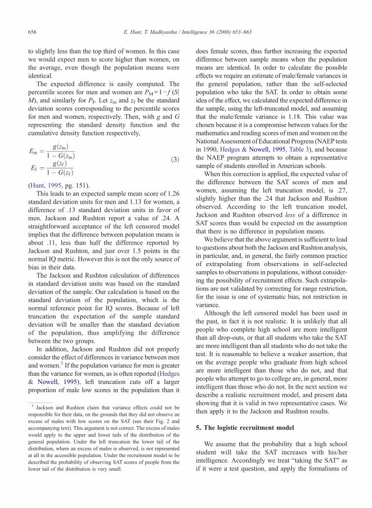
The expected difference is easily computed. Thepercentile scores for men and women are PM=1− f (S|M), and similarly for PF. Let zm and zf be the standarddeviation scores corresponding to the percentile scoresfor men and women, respectively. Then, with g and Grepresenting the standard density function and thecumulative density function respectively,

Em ¼ g zmð Þ1� G zmð Þ

Ef ¼ g zfð Þ1� G zfð Þ

ð3Þ

(Hunt, 1995, pg. 151).This leads to an expected sample mean score of 1.26

standard deviation units for men and 1.13 for women, adifference of .13 standard deviation units in favor ofmen. Jackson and Rushton report a value of .24. Astraightforward acceptance of the left censored modelimplies that the difference between population means isabout .11, less than half the difference reported byJackson and Rushton, and just over 1.5 points in thenormal IQ metric. However this is not the only source ofbias in their data.

The Jackson and Rushton calculation of differencesin standard deviation units was based on the standarddeviation of the sample. Our calculation is based on thestandard deviation of the population, which is thenormal reference point for IQ scores. Because of lefttruncation the expectation of the sample standarddeviation will be smaller than the standard deviationof the population, thus amplifying the differencebetween the two groups.

In addition, Jackson and Rushton did not properlyconsider the effect of differences in variance between menand women.3 If the population variance for men is greaterthan the variance for women, as is often reported (Hedges& Nowel l, 1995), left truncation cuts off a largerproportion of male low scores in the population than it

3 Jackson and Rushton claim that variance effects could not beresponsible for their data, on the grounds that they did not observe anexcess of males with low scores on the SAT (see their Fig. 2 andaccompanying text). This argument is not correct. The excess of maleswould apply to the upper and lower tails of the distribution of thegeneral population. Under the left truncation the lower tail of thedistribution, where an excess of males is observed, is not representedat all in the accessible population. Under the recruitment model to bedescribed the probability of observing SAT scores of people from thelower tail of the distribution is very small.

does female scores, thus further increasing the expecteddifference between sample means when the populationmeans are identical. In order to calculate the possibleeffects we require an estimate of male/female variances inthe general population, rather than the self-selectedpopulation who take the SAT. In order to obtain someidea of the effect, we calculated the expected difference inthe sample, using the left-truncated model, and assumingthat the male/female variance is 1.18. This value waschosen because it is a compromise between values for themathematics and reading scores ofmen and women on theNationalAssessment of Educational Progress (NAEP testsin 1990, H e dg es & Nowell, 1995, Ta b l e 3 ), and becausethe NAEP program attempts to obtain a representativesample of students enrolled in American schools.

When this correction is applied, the expected value ofthe d ifference between the SAT scores of men andwomen, assuming the left truncation model, is .27,slightly higher than the .24 that Jackson and Rushtonobserved. According to the left truncation model,Jackson and Rushton observed less of a difference inSAT scores than would be expected on the assumptionthat there is no difference in population means.

We believe that the above argument is sufficient to leadto questions about both the Jackson and Rushton analysis,in particular, and, in general, the fairly common practiceof extrapolating from observations in self-selectedsamples to observations in populations, without consider-ing the possibility of recruitment effects. Such extrapola-tions are not validated by correcting for range restriction,for the issue is one of systematic bias, not restriction invariance.

Although the left censored model has been used inthe past, in fact it is not realistic. It is unlikely that allpeople who complete high school are more intelligentthan all drop-outs, or that all students who take the SATare more intelligent than all students who do not take thetest. It is reasonable to believe a weaker assertion, thaton the average people who graduate from high schoolare more intelligent than those who do not, and thatpeople who attempt to go to college are, in general, moreintelligent than those who do not. In the next section wedescribe a realistic recruitment model, and present datashowing that it is valid in two representative cases. Wethen apply it to the Jackson and Rushton results.

5. The logistic recruitment model

We assume that the probability that a high schoolstudent will take the SAT increases with his/herintelligence. Accordingly we treat “taking the SAT” asif it were a test question, and apply the formalisms of

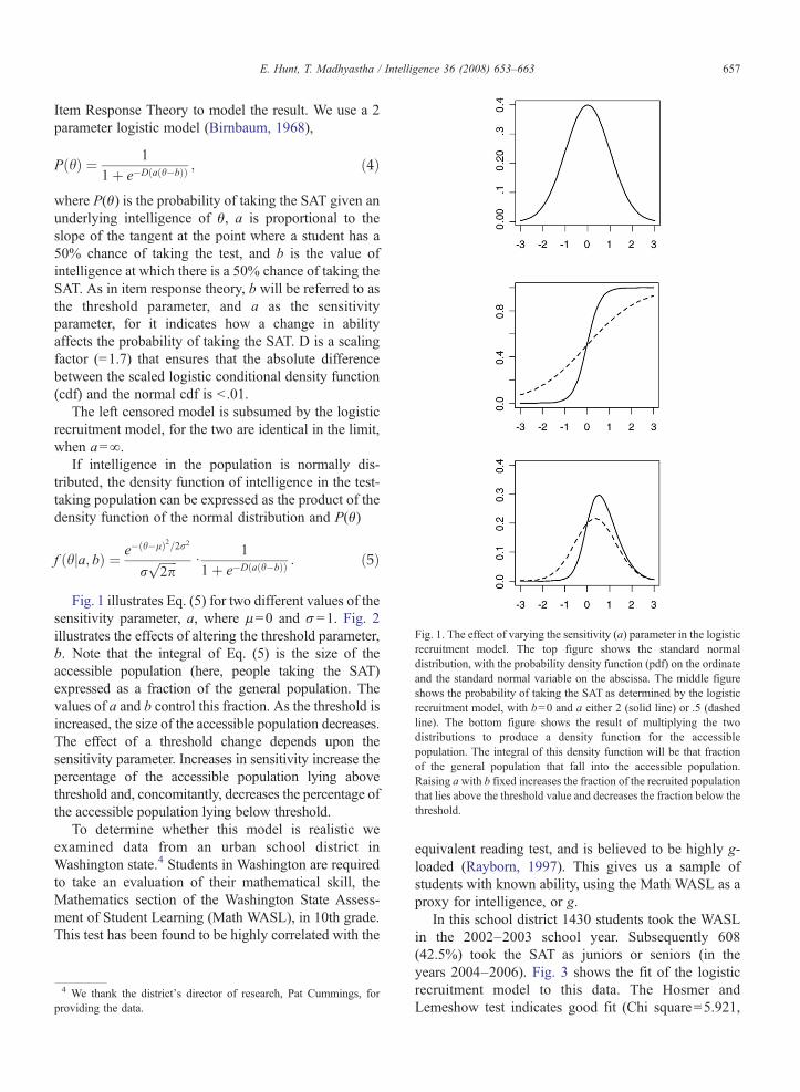
Fig. 1. The effect of varying the sensitivity (a) parameter in the logisticrecruitment model. The top figure shows the standard normaldistribution, with the probability density function (pdf) on the ordinateand the standard normal variable on the abscissa. The middle figureshows the probability of taking the SAT as determined by the logisticrecruitment model, with b=0 and a either 2 (solid line) or .5 (dashedline). The bottom figure shows the result of multiplying the twodistributions to produce a density function for the accessiblepopulation. The integral of this density function will be that fractionof the general population that fall into the accessible population.Raising awith b fixed increases the fraction of the recruited populationthat lies above the threshold value and decreases the fraction below thethreshold.

657E. Hunt, T. Madhyastha / Intelligence 36 (2008) 653–663

Item Response Theory to model the result. We use a 2parameter logistic model (Birnbaum, 1968),

P hð Þ ¼ 1

1þ e�D a h�bð Þð Þ ; ð4Þ

where P(θ) is the probability of taking the SAT given anunderlying intelligence of θ, a is proportional to theslope of the tangent at the point where a student has a50% chance of taking the test, and b is the value ofintelligence at which there is a 50% chance of taking theSAT. As in item response theory, b will be referred to asthe threshold parameter, and a as the sensitivityparameter, for it indicates how a change in abilityaffects the probability of taking the SAT. D is a scalingfactor (=1.7) that ensures that the absolute differencebetween the scaled logistic conditional density function(cdf) and the normal cdf is b .01.

The left censored model is subsumed by the logisticrecruitment model, for the two are identical in the limit,when a=∞.

If intelligence in the population is normally dis-tributed, the density function of intelligence in the test-taking population can be expressed as the product of thedensity function of the normal distribution and P(θ)

f hja; bð Þ ¼ e� h�lð Þ2=2r2

rffiffiffiffiffiffi

2pp d

1

1þ e�D a h�bð Þð Þ : ð5Þ

Fig. 1 illustrates Eq. (5) for two different values of thesensitivity parameter, a, where μ=0 and σ=1. Fig. 2illustrates the effects of altering the threshold parameter,b. Note that the integral of Eq. (5) is the size of theaccessible population (here, people taking the SAT)expressed as a fraction of the general population. Thevalues of a and b control this fraction. As the threshold isincreased, the size of the accessible population decreases.The effect of a threshold change depends upon thesensitivity parameter. Increases in sensitivity increase thepercentage of the accessible population lying abovethreshold and, concomitantly, decreases the percentage ofthe accessible population lying below threshold.

To determine whether this model is realistic weexamined data from an urban school district inWashington state.4 Students in Washington are requiredto take an evaluation of their mathematical skill, theMathematics section of the Washington State Assess-ment of Student Learning (Math WASL), in 10th grade.This test has been found to be highly correlated with the

4 We thank the district's director of research, Pat Cummings, forproviding the data.

equivalent reading test, and is believed to be highly g-loaded (Rayborn, 1997). This gives us a sample ofstudents with known ability, using the Math WASL as aproxy for intelligence, or g.

In this school district 1430 students took the WASLin the 2002–2003 school year. Subsequently 608(42.5%) took the SAT as juniors or seniors (in theyears 2004–2006). Fig. 3 shows the fit of the logisticrecruitment model to this data. The Hosmer andLemeshow test indicates good fit (Chi square=5.921,

Fig. 2. The effect of varying the threshold (b) parameter in the logisticrecruitment model. The top figure shows the standard normaldistribution, with the probability density function (pdf) on the ordinateand the standard normal variable on the abscissa. The middle figureshows the probability of taking the SAT as determined by the logisticrecruitment model, with a=.5 and b either 2 (solid line) or .5 (dashedline). The bottom figure shows the result of multiplying the twodistributions to produce a density function for the accessiblepopulation. The integral of this density function will be the fractionof the general population that fall into the accessible population.Raising b with a fixed a decreases the size of the accessiblepopulation, as a fraction of the general population, and increases thevalues within the accessible population of the variable on whichrecruitment takes place.

Fig. 3. The logistic recruitment model fitted to data from an urbanschool district in Washington State. The relative frequency of takingthe SAT (P(SAT) is shown as a function of a student's MathematicsWASL score. The points represent the fraction of students taking theWASL in a bin of ten students whose WASL scores were within a tenpoint span. The line is the logistic regression of the P(SAT) on theWASL. The best fitting parameters are a=.669 and b=.339.

658 E. Hunt, T. Madhyastha / Intelligence 36 (2008) 653–663

df=8, pb .65). For reference, a score of 400 on theWASL indicates proficiency as established by the statestandards. The parameters are a=.669, b=.339 for allstudents.

We then examined the population ofmales and femalesseparately. The Math WASL was taken by 800 (55.94%)females and 630 (44.06%)males. Fig. 4 shows the logisticregression of the probability of taking the SAT on mathWASL separately for females and males. For females, theHosmer and Lemeshow goodness of fit is Chisquare=5.02, df=8, and pb .75. For males, it is Chisquare=8.56, df=8, and pb .38. The parameter values are

a=.751, b=.172 for females and a=.598, b=.591 formales. This means that the 50% threshold for deciding totake the SATwas lower for women than for men, and thatfor practically all but the lowest levels of the MathWASLwomen were more likely to take the SAT than men.

We then used the logistic recruitmentmodel to calculatethe expected difference in SAT scores in the school inquestion. As before, and as in Jackson and Rushton'sanalysis, the calculations will be in terms of populationstandard deviation units, assuming a population mean ofzero, and no mean differences between men and women.

The expected value of the sample mean for a groupcan be calculated by taking the integral of the product ofEq. (6) at each level of intelligence (θ), multiplied by theθ value, and normalizing by dividing by the expectedfraction of the group that appears in the accessiblepopulation. The a and b parameters used are thosedetermined by fitting the logistic regression model to thegroup equation.

E hð Þ ¼ ∫ e� h�lð Þ2=2r2

rffiffiffiffiffiffi

2pp d

1

1þ e�D a h�bð Þð Þ d hdh

�∫ e� h�lð Þ2=2r2

rffiffiffiffiffiffi

2pp d

1

1þ e�D a h�bð Þð Þ dh:

ð6Þ

We applied Eq. (6) to calculate the expected samplemeans for men and women, using the parameter

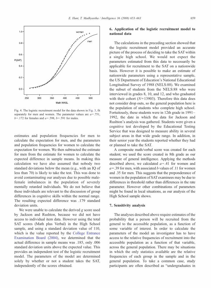
Fig. 4. The logistic recruitment model for the data shown in Fig. 3, fitseparately for men and women. The parameter values are a=.751,b=.172 for females and a=.598, b=.591 for males.

659E. Hunt, T. Madhyastha / Intelligence 36 (2008) 653–663

estimates and population frequencies for men tocalculate the expectation for men, and the parametersand population frequencies for women to calculate theexpectation for women. We then subtracted the estimatefor men from the estimate for women to calculate theexpected difference in sample means. In making thiscalculation we have also assumed that nobody twostandard deviations below the mean (e.g., with an IQ ofless than 70) is likely to take the test. This was done toavoid contaminating our analyses due to possible male-female imbalances in the population of severelymentally retarded individuals. We do not believe thatthese individuals are relevant to the discussion of groupdifferences in cognitive skills within the normal range.The resulting expected difference was .179 standarddeviation units.

We were unable to calculate the derived g score usedby Jackson and Rushton, because we did not haveaccess to individual item data. However using the totalSAT scores (Math plus Verbal) in the High Schoolsample, and using a standard deviation value of 110,which is the value reported by the College EntranceExamination Board (2004), we determined that theactual difference in sample means was .185, only .006standard deviation units above the expected value. Thisprovides an independent test of the logistic recruitmentmodel. The parameters of the model are determinedsolely by whether or not a student takes the SAT,independently of the scores obtained.

6. Application of the logistic recruitment model tonational data

The calculations in the preceding section showed thatthe logistic recruitment model provided an accuratepicture of the process of deciding to take the SATwithina single high school. We would not expect theparameters estimated from this data to necessarily beapplicable for recruitment to the SAT on a nationwidebasis. However it is possible to make an estimate ofnationwide parameters using a representative sample,the US Department of Education's National EducationalLongitudinal Survey of 1988 (NELS:88). We examinedthe subset of students from the NELS:88 who wereinterviewed in grades 8, 10, and 12, and who graduatedwith their cohort (N=13903). Therefore this data doesnot consider drop outs, so the general population here isthe population of students who complete high school.Fortuitously, these students were in 12th grade in 1991–1992, the date in which the data for Jackson andRushton's analysis was gathered. Students were given acognitive test developed by the Educational TestingService that was designed to measure ability in severalsubject areas in that wide grade range. In addition, intheir senior year the students reported whether they hador planned to take the SAT.

A composite math/verbal score was created for eachstudent; we used the score created in 8th grade as ourmeasure of general intelligence. Applying the methodsdescribed above, we calculated a=.41 for women anda=.39 for men, with associated b values of .11 for womenand .35 for men. This suggests that the preponderance ofwomen in the population of SATexaminees may be due todifferences in threshold rather than differences in the rateparameter. However other combinations of parametersmight be found in local situations, as our analysis of theHigh School sample shows.

7. Sensitivity analysis

The analyses described above require estimates of theprobability that a person will be recruited from thegeneral to the accessible population, as a function ofsome variable of interest. In order to calculate theparameters of the model an investigator has to haveaccess to the relative frequencies of recruitment into theaccessible population as a function of that variable,across the general population. There may be situationsin which the only statistics available are the relativefrequencies of each group in the sample and in thegeneral population. To take a common case, studyparticipants are often described as “undergraduates in

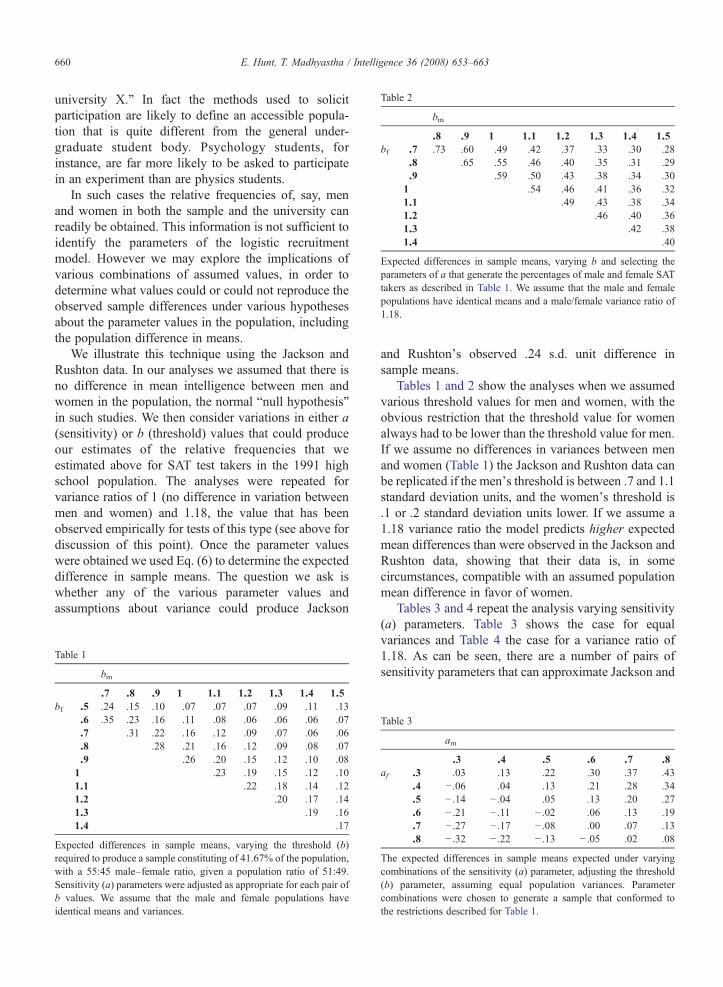
Table 2

bm

.8 .9 1 1.1 1.2 1.3 1.4 1.5bf .7 .73 .60 .49 .42 .37 .33 .30 .28

.8 .65 .55 .46 .40 .35 .31 .29

.9 .59 .50 .43 .38 .34 .301 .54 .46 .41 .36 .321.1 .49 .43 .38 .341.2 .46 .40 .361.3 .42 .381.4 .40

Expected differences in sample means, varying b and selecting theparameters of a that generate the percentages of male and female SATtakers as described in Table 1. We assume that the male and femalepopulations have identical means and a male/female variance ratio of1.18.

660 E. Hunt, T. Madhyastha / Intelligence 36 (2008) 653–663

university X.” In fact the methods used to solicitparticipation are likely to define an accessible popula-tion that is quite different from the general under-graduate student body. Psychology students, forinstance, are far more likely to be asked to participatein an experiment than are physics students.

In such cases the relative frequencies of, say, menand women in both the sample and the university canreadily be obtained. This information is not sufficient toidentify the parameters of the logistic recruitmentmodel. However we may explore the implications ofvarious combinations of assumed values, in order todetermine what values could or could not reproduce theobserved sample differences under various hypothesesabout the parameter values in the population, includingthe population difference in means.

We illustrate this technique using the Jackson andRushton data. In our analyses we assumed that there isno difference in mean intelligence between men andwomen in the population, the normal “null hypothesis”in such studies. We then consider variations in either a(sensitivity) or b (threshold) values that could produceour estimates of the relative frequencies that weestimated above for SAT test takers in the 1991 highschool population. The analyses were repeated forvariance ratios of 1 (no difference in variation betweenmen and women) and 1.18, the value that has beenobserved empirically for tests of this type (see above fordiscussion of this point). Once the parameter valueswere obtained we used Eq. (6) to determine the expecteddifference in sample means. The question we ask iswhether any of the various parameter values andassumptions about variance could produce Jackson

Table 1

bm

.7 .8 .9 1 1.1 1.2 1.3 1.4 1.5bf .5 .24 .15 .10 .07 .07 .07 .09 .11 .13

.6 .35 .23 .16 .11 .08 .06 .06 .06 .07

.7 .31 .22 .16 .12 .09 .07 .06 .06

.8 .28 .21 .16 .12 .09 .08 .07

.9 .26 .20 .15 .12 .10 .081 .23 .19 .15 .12 .101.1 .22 .18 .14 .121.2 .20 .17 .141.3 .19 .161.4 .17

Expected differences in sample means, varying the threshold (b)required to produce a sample constituting of 41.67% of the population,with a 55:45 male–female ratio, given a population ratio of 51:49.Sensitivity (a) parameters were adjusted as appropriate for each pair ofb values. We assume that the male and female populations haveidentical means and variances.

and Rushton's observed .24 s.d. unit difference insample means.

Tables 1 and 2 show the analyses when we assumedvarious threshold values for men and women, with theobvious restriction that the threshold value for womenalways had to be lower than the threshold value for men.If we assume no differences in variances between menand women (Table 1) the Jackson and Rushton data canbe replicated if the men's threshold is between .7 and 1.1standard deviation units, and the women's threshold is.1 or .2 standard deviation units lower. If we assume a1.18 variance ratio the model predicts higher expectedmean differences than were observed in the Jackson andRushton data, showing that their data is, in somecircumstances, compatible with an assumed populationmean difference in favor of women.

Tables 3 and 4 repeat the analysis varying sensitivity(a) parameters. Table 3 shows the case for equalvariances and Table 4 the case for a variance ratio of1.18. As can be seen, there are a number of pairs ofsensitivity parameters that can approximate Jackson and

Table 3

am

.3 .4 .5 .6 .7 .8af .3 .03 .13 .22 .30 .37 .43

.4 − .06 .04 .13 .21 .28 .34

.5 − .14 − .04 .05 .13 .20 .27

.6 − .21 − .11 − .02 .06 .13 .19

.7 − .27 − .17 − .08 .00 .07 .13

.8 − .32 − .22 − .13 − .05 .02 .08

The expected differences in sample means expected under varyingcombinations of the sensitivity (a) parameter, adjusting the threshold(b) parameter, assuming equal population variances. Parametercombinations were chosen to generate a sample that conformed tothe restrictions described for Table 1.

Table 4

am

.3 .4 .5 .6 .7 .8af .3 .19 .31 .42 .51 .59 .66

.4 .10 .22 .33 .43 .51 .58

.5 .02 .14 .25 .35 .43 .50

.6 − .05 .07 .18 .28 .36 .43

.7 − .11 .01 .12 .21 .30 .37

.8 − .17 − .04 .07 .16 .24 .31

The analysis of Table 3 repeated assuming a variance ratio of 1.18.

661E. Hunt, T. Madhyastha / Intelligence 36 (2008) 653–663

Rushton's result and, if the 1.18 variance ratio isaccepted, a number of pairs for which the expectedmean difference exceeds that found by Jackson andRushton.

Tables 1–4 and the different assumptions aboutvariance ratios can be thought of as analogous to theconventional procedure of evaluating empirical results bycomparing them towhat would be expected under the nullhypothesis that there is no difference between groups. Theonly logical difference is that in the conventionalprocedure one determines the region of a one-dimensionalspace (the population mean) that could give rise to theobserved effects. In the analysis here we consider whatregion of the five dimensional space (parameter valuesand the variance ratio) might have produced the observedresults. In terms of familiar statistics, we are dealing withconfidence regions instead of confidence intervals.

The sensitivity analysis presented here considersonly the case of the “null hypothesis,” that there are nodifferences in population means. It is also possible todetermine confidence regions under alternative hypoth-eses about population means. For instance, Jackson andRushton state (and we agree) that it would be interestingto know if their results could be replicated in moregeneral populations. Suppose we take as an alternativehypothesis the assumption that the population means areindeed approximately those observed in Jackson andRushton's sample. This hypothesis is also interestingbecause it approximates a hypothesis about differencesin g in men and women that has been put forward byother inves tigators (Lynn & Irwing, 2004a,b) .

We have explored this possibility, and found that ifthe alternative hypothesis is true there are manyparameter combinations for which the predicted differ-ence in sample means is greater than that observed byJackson and Rushton. This finding is not surprising, for,as Tables 1–4 show, there are combinations of parametervalues that lead to a greater-than-observed difference insample means without assuming a difference inpopulation means. This is particularly true for anassumed variance ratio of 1.18, which we regard asthe most likely value for a test similar to the SAT. For

studies using different types of tests, such as the RavenMatrices reports analyzed by Lynn and Irwing (2004a,b), a different assumption might be appropriate. Whatthis means in terms of generalizing their results (oranyone else's) can only be answered by conductinganalyses similar to the ones we have reported here forthe Jackson and Rushton data.

We repeat our major conclusion. By combining anobserved difference with a recruitment model we maydetermine what the characteristics of the generalpopulation would have to be to give rise to observationsin a sample from the accessible population. While theprocedures we describe here are, insofar as we know,original, our use of the logistic regression model is inprinciple no different from the use of the normaldistribution in the common procedures of placingconfidence limits around sample results or investigatingthe compatibility of observed results with variousalternative hypotheses.

8. Discussion

Our results have two implications: for the interpreta-tion of sample results in general, and for the specificcase that we used as an example, male–femaledifferences in intelligence.

We regard the first implication as by far the mostimportant. However we would like to dispose of theissue concerning male–female differences first. Webelieve that the Jackson and Rushton study cannot beused to draw the conclusion that men exceed women ingeneral intelligence, in the population as a whole.However, conditional upon accepting their identifica-tion of a general factor on the SAT with ‘generalintelligence,' which is not unreasonable, the Jacksonand Rushton study does provide evidence for aconclusion that in the population of university appli-cants men have higher average scores than women. Thismore limited conclusion is not trivial. For instance,Jackson and Rushton's data could validly be used toargue that, given SAT scores, women should beexpected to have lower grades in college than men. Tothe extent that this is not true (and it generally is not, asindicated by a number of studies) other factors, notevaluated by the SAT, must be determining grades.Speculating about what these factors are would take usfar beyond the present discussion.

We now turn to the issue of recruitment moregenerally. We believe that the logistic recruitment modelis a good model of a situation in which the probability ofrecruitment can reasonably be ordered along somevariable of interest. Ordering the variable “probability of

662 E. Hunt, T. Madhyastha / Intelligence 36 (2008) 653–663

preparing to continue education beyond high school” byvariables relating to intelligence, grades, or socio-economic status are obvious candidates for analysis bythe logistic recruitment model.

On the other hand, we do not believe that the logisticrecruitment model applies to all situations. Our moregeneral point is that some recruitment process will apply,and before interpreting a finding consideration has to begiven to the recruitment process. We can think ofrecruitment processes in which probability of recruitmentmight be negatively related to intelligence, or even non-monotonically related, but still reflect an orderly process.

As an example of what is likely to be a non-monotoniccase, consider the many studies in which the participantsare drawn from enlistees in the US Armed Services.Enlistment in the military is related to intelligence in twoseparate ways. People with low scores on cognitiveaptitude tests (such as the Armed Services QualificationTest-AFQT) are either disqualified or, depending upon theneed for enlistees at the time, unlikely to be recruited.Those individuals in the general population who, if theytook the AFQT, would have obtained very high scores arenot likely to volunteer for enlistment; preferring to pursueother options, including enrollment in colleges anduniversities. We conjecture that a model of the militaryrecruitment process into the US Armed Services wouldhave to establish some point on an intelligence test scalethat represents individuals most likely to enlist, with theprobability of enlistment falling off from that point,possibly in an asymmetric fashion.

Readers may think of other models, for othersituations. The point is that recruitment effects can besubstantial. Furthermore, it will often be the case that thepresence of substantial recruitment effects can bedetected by a rather superficial analysis of the data. Toillustrate this we consider two more studies of male–female differences.

Lynn and Irwing (2004b) report a difference betweenmen and women, in favor of men, on the Raven Matrixtest. From this study they generalize to the population ofcollege students. Their sample consisted of 1807 menand 415 women enrolled at Texas Agricultural andMechanical University (Texas A&M) during the 1990s.The sample was not collected by Lynn and Irwingthemselves, and they provide no further informationconcerning the sampling procedure.

Examination of the statistical analysis of enrollmentsprovided on the Texas A&M website shows that over thisperiod the enrollments of men and women wereapproximately equal, so the sample was clearly not arandom sample of that university's student body, let aloneof American university students in general. Given how

little we know about the construction of the sample, wehave noway to construct a recruitmentmodel. For instance,in this case there is no compelling reason to believe that therecruitment process for women would necessarily havebeen more selective with respect for intelligence than theprocess for men. In fact, it might have been the reverse.Wesimply do not know. What we do know, however, is thatsubstantial and differentiated recruitment must haveoccurred, because the male:female ratio in the samplewas so disparate from that in the university at the time.

The same authors report a meta-analysis of studies ofmale–female differences in intelligence in several coun-tries (Ly n n & Irwing, 2004a). It would not be appropriatehere to go into detail about this meta-analysis, as ourpurpose is only to show how suspicious some (not all) oftheir data points are. The ratio of men to women in theirBrazilian sample was 2.35:1. Either Brazil has an unusualpopulation, or a recruitment model should be investigated,or the data point should be regarded as of low qualityindeed. Similarly, their male–female ratios for studies inFrance, England, and the US (two studies combined) are,respectively, .70, .82, and .80. In these developedcountries wewould not expect such ratios unless samplingwas restricted to senior citizens, a population where thereis a preponderance of women. Some consideration ofrecruitment effects is obviously required.

We do not believe that the problems discussed hereoccur solely in the study of male–female differences, orfor that matter solely in the study of intelligence.Elsewhere one of us has pointed out that recruitmenteffects are common in the study of differences in traitsbetween groups, and that failing to consider them canlead to errone ous conclu sions ( Hunt & Carlso n, 2007).Here we have illustrated one possible solution to therecruitment problem. We think it has widespread but notuniversal applicability. We encourage others to developmodels for other situations. We also believe that, in theabsence of modeling, authors should provide, andeditors and reviewers should insist upon, much moreinformation about sampling than statements like “parti-cipants were university students…”. This is especiallythe case when, as in the studies cited here, examinationsof statistics on group participation rate indicate that theaccessible population was unlikely to be a representativesample of the general population.

References

Birnbaum, A. (1968). Some latent trait models and their use ininferring an examinee's ability. In F. M. Lord, & M. R. Novick(Eds.), Statistical theories of mental test scores Reading, Mass.:Addison-Wesley Publishing.

663E. Hunt, T. Madhyastha / Intelligence 36 (2008) 653–663

College Entrance Examination Board (2004). College-bound seniors:A profile of SAT program test-takers. Retrieved November 14,2007, from http://www.collegeboard.com/prod_downloads/about/news_info/cbsenior/yr2004/2004_CBSNR_total_group.pdf

Hedges, L. V., & Nowell, A. (1995). Sex differences in mental testscores, variability, and numbers of high-scoring individuals.Science, 270, 365−367.

Hunt, E. (1995). Will we be smart enough: A cognitive analysis of thecoming workforce. New York: Russell Sage Foundation.

Hunt, E., & Carlson, J. (2007). Considerations relating to the study ofgroup differences in intelligence. Perspectives in PsychologicalScience, 2(2), 194−213.

Jackson, D. N., & Rushton, J. P. (2006). Males have greater g. Sexdifferences in mental ability from 100,000 17–18-year-olds on theScholastic Assessment Test. Intelligence, 34(5), 479−486.

Jensen, A. R. (1998). The g factor: the science of mental ability.Human evolution, behavior, and intelligence. Westport, CT:Praeger.

Kanazawa, S. (2006). IQ and the wealth of states. Intelligence, 34(6),593−600.

Losen, D. J., Orfield, G., Wald, J., & Swanson, C. B. (2004). Losingour future: how minority youth are being left behind by thegraduation rate crisis. Cambridge, MA: Civil Rights Project,Harvard University.

Lynn, R., & Irwing, P. (2004). Sex differences on the progressivematrices: A meta-analysis. Intelligence, 32(5), 481−498.

Lynn, R., & Irwing, P. (2004). Sex differences on the advancedprogressive matrices in college students. Personality and Indivi-dual Differences, 37(1), 219−223.

National Center for Education Statistics (2006). Digest of educationstatistics. Retrieved August 7, 2007, from http://nces.ed.gov/programs/digest/

Rayborn, R. R. (1997). An examination of content and constructvalidity for the Washington State assessment of student learninggrade 4 math test. Washington Educational Research Association,Winter Conference, 1997.