recovering industrial waste heat by the means of ... · recovering industrial waste heat by the...
TRANSCRIPT

Recovering Industrial Waste Heat by the Means ofThermoelectricity
Spring 2010
Department of ChemistryNorwegian University of Science and Technology


I
Declaration
I declare that the work presented in this thesis has been accomplished independentlyand in agreement with “Reglement for sivilarkitekt- og sivilingeniøreksamen”.
Trondheim, June 27, 2010
Marit Takla


III
Summary
The main objectives of this thesis were to establish testing procedures to test perfor-mances of commercially available thermoelectric modules and to build a thermoelectricpower generator demonstration unit. The purpose of the demonstration unit was to gen-erate electricity from energy dissipated as thermal radiation from liquid silicon coolingin the casting area at the silicon plant of Elkem Salten.
An experimental set up has been constructed to test the performance of a thermoelectricmodule operating as a power generator. The polarisation curves, where module potentialis plotted as a function of current, was used as a measure for module performance. Weobtained polarisation curves for different temperature differences across the module.The experimentally determined performances were found to be poorer than performancedata provided by the supplier and underlines the importance of testing performances ofcommercially available modules. From the polarisation curves we determined the internalresistance of the module and found this to increase by increasing temperature. The emfof the module was plotted as a function of temperature difference across the module andthe emf appeared to be a linear function of the temperature difference. We determinedthe Seebeck coefficient for the semiconductor pairs that constitutes the module from theline slope.
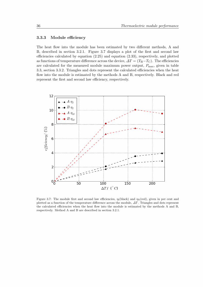
The first and second law efficiency for the thermoelectric device has been estimated.We had to know the heat flow into the module in order to calculate the efficiency, andestimated this by two methods, A and B. In method A, the heat flow was estimatedfrom cooling water volume flow and the cooling water temperature at outlet and inletto the water cooled heat sink in the experimental set up. By method B, we calculatedthe heat flow from module thermal conductivity and temperature difference across themodule. The heat flow estimated by the two methods differed which may be explainedby a heat leakage in the set up. The first and second law efficency were estimated tobe in the range 2 % - 4 % and 6 % - 10 %, respectively, depending on the temperaturedifference across the module and the method used to determine the heat flow. The firstlaw efficiency seemed to increase linearly with temperature while a maximum for thesecond law efficiency was observered. This indicates that the degree of reversibility istemperature dependent.
A calorimeter has been used to measure the heat supplied by a thermoelectric module

(operated as a heat pump) to the surroundings. This heat was interpreted as the lostwork of the device. The aim of the calorimetric study was to investigate the contri-butions to the losses in a thermoelectric device. We determined the lost work for twoexperimental conditions; for the condition of changing the voltage applied to the devicestepwise and for the condition of keeping the current constant while changing the tem-perature difference across the device. We found that work is lost in a thermoelectricdevice due to heat conduction and Joule heating. In order to minimize the lost workin a thermoelectric device, the thermal conductivity and the ohmic resistance of thesemiconductors must be minimized.
In the calorimetric study, we also measured the device internal resistance as a functionof device temperature. The internal resistance was found to increase with increasingtemperature which was in agreement with the findings from the performance testing.
We established a model for determining the module Seeebeck coefficient from data ob-tained from the calorimetric study. The value for the Seebeck coefficient determined bythis calorimetric method was not in agreement with the Seebeck coefficient determinedfrom performance testing data which. We suspect that the model may be too roughor incorrect and it should therefore be further improved to see if the two methods canestimate corresponding values for the coefficient.
A thermoelectric power generator demonstration unit has been constructed in coopera-tion with Termo-Gen AB (Sweden) who also built the demonstration unit. It has beendesigned to yield 100 W gross, assuming a minium heat flux of 15 kW/m2 and a max-imum heat flux of 22.5 − 25 kW/m2 into the hot side of the generator. Unfortunately,there was no time for testing the demonstration unit as the delivery of the unit wasseveral weeks delayed.

V
Sammendrag
Hovedmalene for denne oppgaven var a etablere prosedyrer for a teste yteevnen til ter-moelektriske moduler samt a bygge en demonstrasjonsenhet av en termoelektrisk gen-erator. Formalet med demonstrasjonsenheten var a bruke den til a generere strøm fravarme avgitt fra flytende silisium under støping ved silisiumverket Elkem Salten.
Et forsøksoppsett har blitt bygget for a kunne bestemme ytelsen til en termoelektriskmodul (som genererer strøm) som en funksjon av temperaturforskjell over modulen. Sommal for ytelse har vi brukt polarisasjonskurver som er kurver hvor modulens potensialplottes som en funksjon av strøm. Den eksperimentelt bestemte ytelsen til en modul vardarligere enn ytelsen oppgitt fra leverandør. Dette understreker at det er viktig a testeytelsen til moduler opp imot data oppgitt fra leverandør. Modulens indre motstandble bestemt utifra polarisasjonskurvene og funnet til a øke med økende temperatur.Fra polarisasjonskurvene har vi ogsa bestemt modulens emf og ved a plotte denne mottemperaturforskjellen over modulen har vi observert at den ser ut til a øke lineært medtemperaturforskjellen. Denne grafen har vi brukt til a estimere Seebeck koeffisienten tilhalvlederparene som utgjør modulen.
Videre har vi estimert modulens første og andre lovs virkningsgrad. For a estimere dissematte varmestrømmen inn i modulen estimeres. Denne varmestrømmen har blitt es-timert for tilfellet nar det ikke gar noen elektrisk strøm igjennom modulen ved to ulikemetoder, A og B. Ved metode A har varmestrømmen blitt estimert fra oppvarming avkjølevannet til den kalde siden i forsøksoppsettet og gjort ved a male utløps- og innløp-stemperaturen til kjølevannet samt volumstrømmen. Ved metode B har varmestrømmenblitt beregnet utifra modulens termiske ledningsevne (bestemt eksperimentelt) og tem-peraturforskjell over modulen. Varmestrømmen estimert ved metode A er høyere ennvarmestrømmen estimert ved metode B og forsøksoppsettet bør forbedres for a se omde to metodene vil gi bedre samsvar. Modulens første og andre lovs virkningsgrad harblitt estimert til a være henholdsvis mellom 2 % - 4 % og 6% - 10%, avhengig av metodebrukt til a estimere varmestrømmen inn i modulen og temperaturforskjell over modulen.Første lovs virkningsgrad ser ut til a være en lineær funksjon av temperaturforskjellover modulen, for andre lovs virkningsgrad er det observert et maksimum. Dette maksi-mumet kan tolkes som at graden av reversibilitet for modulen ikke er en lineær funksjonav temperatur.

Et kalorimeter har blitt brukt til a male varme avgitt fra en termoelektrisk modul sombrukes som en varmepumpe. Denne varmen har blitt tolket til a være lik det taptearbeidet til modulen. Hensikten med a male denne varmen var a undersøke bidragenetil tapt arbeid i en termoelektrisk modul. Tapt arbeid ble bestemt ved to ulike forsøks-betingelser; spenningen patrykt modulen ble endret trinnvis og strømmen ble holdtkonstant samtidig som temperaturforskjellen over modulen ble endret trinnvis. Resul-tatene viser at bade Joule-effekten og varmeledning ser ut til a være viktige bidrag tiltapt arbeid, hvilket betyr at indre motstand og termisk ledningsevne bør minimeres fora minimere tapt arbeid.
Kalorimeteroppsettet ble ogsa brukt til a bestemme modulens indre motstand som enfunksjon av temperatur. Den indre motstanden ble funnet til a øke med en økning itemperatur som samsvarer med observasjonene fra ytelesesforsøkene.
En modell ble etablert for a estimere Seebeck koeffisienten til halvlederene i modulenfra kalorimeterdata. Seebeck koeffisienten som ble bestemt med denne modellen var enstørrelsesorden større enn den som ble estimert fra ytelsesforsøkene. Dette kan tyde paat modellen er for grov og eventuelt ogsa feil, dette bør undersøkes nærmere.
En demonstrasjonsenhet av en termoelektriske generator har blitt til i samarbeid medTermo-Gen AB (Svergie). Disse har ogsa bygget den. Den er designet til a levere100 W brutto, forutsatt at varmefluksen inn i generatoren er mellom 15kW/m2 og 22.5−25kW/m2. Det ble ikke tid til a teste generatoren ettersom den var flere uker forsinketog fortsatt ikke var levert nar denne oppgaven gikk i trykken.

VII
Preface
This thesis concludes the five year Master’s degree program in Chemical Engineeringand Biotechnology at the Norwegian University of Science and Technology (NTNU).This thesis is submitted to the Department of Chemistry, Faculty of Natural Sciencesand Thecnology at NTNU as a partial fulfillment of the requirements for the degree ofMaster of Technology (M. Tech).
This thesis work was carried out between 18 th of January 2010 and 28 th of June 2010at NTNU under the supervision of Professor Signe Kjelstrup, Professor Leiv Kolbeinsenand Dr. Odne Stokke Burheim.
This work is based on a previous project that was conducted autum 2009, and both worksare performed as sub-projects of the NFR founded competence building project FugitiveEmissions of Materials and Energy (FUME). In the previous work, we investigated theopportunity for generating power from radiation waste heat by means of thermoelectric-ity. The focus of the project was the casting area at the silicon plant of Elkem Saltenwhere liquid silicon is the source of radiation. We looked at the opportunity for usingcommercially available thermoelectric devices to convert a part of this heat into electricpower that could power a suction fan in the casting area.


IX
Acknowledgements
First of all I would like to thank Professor Signe Kjelstrup and Professor Leiv Kolbeinsenfor giving me the opportunity to join the work on the project Energy emissions that is asub-project of the FUME project. I would also like to thank Dr. Odne Stokke Burheimfor helping me with the practical work, for his enthusiasm and long discussions in hisoffice.
I would like to thank the people at the local workshop at NTNU that have made theparts for the new experimental set up constructed during this work. I would also liketo thank Lennart Holmgren at Termo-Gen AB who has built the thermoelectric powergenerator reported in this work.


XI
List of Symbols
Roman symbols
∆Si entropy change J K−1
dSirrdt total entropy procuction J K−1s−1
Ω cross sectional area semiconductors m2
Q heat flow rate W
T average temperature K
V volume flow rate m3s−1
cp specific heat capacity at constant pressure J kg−1 K−1
E electromotive force, emf V
F Faradays constant 96500 C mol−1
I current A
j current density A m−2
J ′q flux of measurable heat Jm−2s−1
K total thermal conductivity. Linked to specific thermal conductivity as K = λ AdxW
K−1
l length m
Ljj main coefficient
Ljk phenomenological coefficient for coupling of fluxes j and k

N number of semiconductor pairs
P power delivered to an external load W
R internal resistance ohm
RL resistance of external load ohm
S∗ transported entropy J K−1 mol−1
T absolute temperature K
t time s
V volume m3
w work done on the system J
wlost work lost in an irreversible process J
Zc thermoelectric figure of merit
Greek symbols
∆ change in quantity or variable
ηI first law efficiency
ηC Carnot efficiency
ηdevice thermoelectric device efficiency
ηII second law efficiency
ηs seebeck coefficient V K−1
γ embodies the parameters of the materials
κ electrical conductivity S m−1
λ thermal conductivity W K−1 m−1
Ω surface area m2
φ electric potential V
π peltier coefficient J mol−1

ρ density kg m−3
σ local entropy production Js−1K−1m−3
Superscripts and subscripts
0 super- or subscript reffering to the surroundings
C subscript meaning cold side
H subscript meaning hot side
id super- or subscript meaning the ideal case
m subscript meaning module
n super- or subscript meaning n-type semiconductor
p super- or subscript meaning p-type semiconductor
surr surroundings
sys system
w super-or subscript meaning water

XV
Contents
1 Introduction 11.1 The Elkem Salten Case study . . . . . . . . . . . . . . . . . . . . . . . . . 2
1.1.1 The Silicon Production . . . . . . . . . . . . . . . . . . . . . . . . 21.1.2 The casting process . . . . . . . . . . . . . . . . . . . . . . . . . . 6
1.2 Project objectives and outline . . . . . . . . . . . . . . . . . . . . . . . . . 8
2 Thermoelectricity 92.1 Thermoelectric devices . . . . . . . . . . . . . . . . . . . . . . . . . . . . . 112.2 Practical application of thermoelectric devices . . . . . . . . . . . . . . . . 132.3 Commerically available thermoelectric devices . . . . . . . . . . . . . . . . 15
2.3.1 New materials . . . . . . . . . . . . . . . . . . . . . . . . . . . . . 162.4 Thermodynamics of thermoelectric devices . . . . . . . . . . . . . . . . . . 17
2.4.1 Coupling of heat and charge transport . . . . . . . . . . . . . . . . 172.4.2 Potential expression . . . . . . . . . . . . . . . . . . . . . . . . . . 182.4.3 Power output . . . . . . . . . . . . . . . . . . . . . . . . . . . . . . 202.4.4 The efficiency of a thermoelectric generator . . . . . . . . . . . . . 21
3 Thermoelectric module performance 253.1 Experimental . . . . . . . . . . . . . . . . . . . . . . . . . . . . . . . . . . 26
3.1.1 Experimental setup . . . . . . . . . . . . . . . . . . . . . . . . . . 263.2 Procedure . . . . . . . . . . . . . . . . . . . . . . . . . . . . . . . . . . . . 28
3.2.1 Module efficiency . . . . . . . . . . . . . . . . . . . . . . . . . . . . 283.3 Results . . . . . . . . . . . . . . . . . . . . . . . . . . . . . . . . . . . . . . 31
3.3.1 Module potential . . . . . . . . . . . . . . . . . . . . . . . . . . . . 313.3.2 Module power output . . . . . . . . . . . . . . . . . . . . . . . . . 343.3.3 Module efficiency . . . . . . . . . . . . . . . . . . . . . . . . . . . . 36
4 Calorimetric study of a thermoelectric device operating in Pelitiermode 394.1 Experimental . . . . . . . . . . . . . . . . . . . . . . . . . . . . . . . . . . 39
4.1.1 Apparatus and experimental setup . . . . . . . . . . . . . . . . . . 394.1.2 Procedure . . . . . . . . . . . . . . . . . . . . . . . . . . . . . . . . 42
4.2 Results . . . . . . . . . . . . . . . . . . . . . . . . . . . . . . . . . . . . . . 48

4.2.1 Experiment type I . . . . . . . . . . . . . . . . . . . . . . . . . . . 484.2.2 Experiment type II . . . . . . . . . . . . . . . . . . . . . . . . . . . 494.2.3 Experiment type III . . . . . . . . . . . . . . . . . . . . . . . . . . 524.2.4 Seebeck coefficient . . . . . . . . . . . . . . . . . . . . . . . . . . . 53
5 Thermoelectric power generator demonstration unit 555.1 Demonstration unit . . . . . . . . . . . . . . . . . . . . . . . . . . . . . . . 555.2 Testing procedure . . . . . . . . . . . . . . . . . . . . . . . . . . . . . . . . 58
6 Discussion 596.1 Performance testing . . . . . . . . . . . . . . . . . . . . . . . . . . . . . . 59
6.1.1 Module potential . . . . . . . . . . . . . . . . . . . . . . . . . . . . 596.1.2 Module power output . . . . . . . . . . . . . . . . . . . . . . . . . 616.1.3 Module efficiency . . . . . . . . . . . . . . . . . . . . . . . . . . . . 62
6.2 Calorimetric studies . . . . . . . . . . . . . . . . . . . . . . . . . . . . . . 646.2.1 Experiment type I . . . . . . . . . . . . . . . . . . . . . . . . . . . 646.2.2 Experiment type II . . . . . . . . . . . . . . . . . . . . . . . . . . . 646.2.3 Experiment type III . . . . . . . . . . . . . . . . . . . . . . . . . . 666.2.4 Seebeck coefficient . . . . . . . . . . . . . . . . . . . . . . . . . . . 66
6.3 Further work . . . . . . . . . . . . . . . . . . . . . . . . . . . . . . . . . . 67
7 Conclusions 69
A Data for the thermoelectric module TEP-1265-1.5 75A.1 Specifications of semiconductor pairs . . . . . . . . . . . . . . . . . . . . . 75A.2 Module specifications . . . . . . . . . . . . . . . . . . . . . . . . . . . . . . 76A.3 Semiconductor properties . . . . . . . . . . . . . . . . . . . . . . . . . . . 80
B Module performance 83B.1 Experimental setup . . . . . . . . . . . . . . . . . . . . . . . . . . . . . . . 83B.2 Raw data . . . . . . . . . . . . . . . . . . . . . . . . . . . . . . . . . . . . 84B.3 Cooling water volume flow . . . . . . . . . . . . . . . . . . . . . . . . . . . 89
C Calorimetric study 91C.1 Experimental set up . . . . . . . . . . . . . . . . . . . . . . . . . . . . . . 91C.2 Raw data for calorimetric studies . . . . . . . . . . . . . . . . . . . . . . . 93
C.2.1 Experiment type II . . . . . . . . . . . . . . . . . . . . . . . . . . . 93C.2.2 Experiment type III . . . . . . . . . . . . . . . . . . . . . . . . . . 99
1
Chapter 1
Introduction
The world’s energy demand increases, driven by population growth and increase in livingstandards [1] and at the same time is global warming recognized as our most seriousenvironmental problem [2]. This makes it necessary to optimize the utilization of energyand encourages scientists and engineers to explore untapped energy sources. Energydissipated as heat into the surroundings is the lost work of a process [3] and this energybecomes unavailable for future utilization. This waste heat represents an untappedenergy source and it’s exploitation will contribute to improve the energy efficiency ofmany processes.
The metalurgical industry is known for its high energy use per unit produced metal;about 13 kWh is needed per kilogram of aluminium produced [4] and about the sameamount is needed per kilogram of silisium produced [5]. About half of the energy inputto Norwegian ferro alloy furnaces is preserved in the metal and the rest leaves the processas varoius heat losses [6]. The total loss is of the same order of magnitude as the totalelectrical input to the process and the possibility for recovering a portion of this is thusof great interest.
Thermoelectricity is about the interconverison of heat and electricity and represents anopportunity for the direct conversion of heat into electricity. Solid state thermoelectricdevices are units based on semiconductors that directly convert a heat flow into electricityor it can be used for heating/cooling applications. We explore the possibillity for usingcommercially available solid state thermoelectric devices for recovering industrial wasteheat. The long range aim is to recover energy dissipated as heat from liquid siliconduring casting at the slicon plant of Elkem Salten.

2 Introduction
1.1 The Elkem Salten Case study
Elkem Salten is one of the silicon plants in the Elkem group and it is located at Salten,about 80 kilometers from Bodø. The plant has been in operation since 1967 and is todayone of the world’s largest and most modern silicon plants. Ferrosilicon with high siliconcontent (typically 97%) and Microsilica R© are the main products [7]. Figure 1.1 displaysa picture of the casting area at Elkem Salten.
Figure 1.1: The casting area at Elkem Salten [7].
1.1.1 The Silicon Production
Silicon is the most common metalloid (semi metal) and it was recognized as an elementin the early nineteenth century. It is the second-most abundant element in the earth’scrust after oxygen. In nature, it exists almost exclusively in combination with oxygen assilicon dioxide and silicates. It is esimated that the earth’s crust contains about 28 percent silicon bound as silicates and silicon dioxide [5].
Silicon is utilized in the metallurgical industry in alloying and deoxidation (binding andremoving of oxides and oxygen) of steel and cast iron, and in alloying of other metals.It is a raw material in the chemical industry and in the semiconductor industry [5].
Silicon is commercially prepared by reduction of silicon dioxide with carbon in an elec-trical arc furnace. The reduction reaction can be written in an idealized form as [5]:
SiO2(s) + 2C(s) = Si(s) + 2CO(g) (1.1)
Figure 1.2 is a schematic drawing illustrating the silicon production process with energyrecovery.
The electric arc furnace is the core of the silicon plant. The size of a furnace is determinedby the electrical power, which can be in the range of less than 10MW and up to about

The Elkem Salten Case study 3
Figure 1.2: A typical silicon metal plant with off-gas cleaning system and energy recovery system. Seetext for more thorough explanation. [5]

4 Introduction
40MW [8]. The pot size of a typical arc furnace is around 10 meter in diameters. Usually,the arc furnaces are water cooled. The raw materials silicon dioxide and carbon are addedto the furnace at the top, and is called the charge material. Production of silicon is anenergy intensive process, requiring temperatures above 1800 C. These temperaturesare achieved by adding large amounts of electric energy. Three electrodes are submergedinto the charge and supply a three phase current. The supplied current heats the hottestpart of the charge up to about 2000C. At this temperature silicon dioxide is reducedto molten silicon. The liquid silicon is tapped from the bottom of the furnace. Aftertapping, the liquid silicon is refined by slag treatment or gas purging. Then the liquidsilicon is poured into suitable moulds, allowed to cool down and then crushed to thedesired sizes. Most plants use 11-13kWh per kilogram of silicon metal produced [5].
The off-gas from the furnace is captured into the gas-cleaning system and filtered. Thedust in the filter consists mainly of SiO2 particles, also named condensed silica fume,which can be used as filler material in concrete, ceramics, rubber etc. [5]. Elkem Siliconsells this product under the trade name Microsilica R©, as mentioned.

The Elkem Salten Case study 5
Dissipated energy and recovery
In a 10 MW furnace, electrical energy accounts for about 45 % of the total energysupplied to the process and chemical energy from the charge materials accounts for therest. About 70 % of the total energy supplied to the process is dissipated as heat [8]into the surroundings. The energy into and out of the process is illustrated in Figure1.3. Available energy is lost as thermal energy in the cooling water, in the off-gass,by radiation and convection from the furnace and from the cooling process of the theliquid metal. The heat content of the cooling water leaving the process correspondsto about 28 % of the electric input to a 10 MW furnace while the heat content in theoff-gas corresponds to about 50 % of the total energy input to the process for a 10MW furnace [9]. One way of increasing the energy efficiency for the silicon productionprocess is to install energy recovery systems. The off-gas temperature is in the rangerange from 200C to 700C [8], which makes the thermal energy in the off-gas suitablefor electric energy conversion using a steam turbine and generator system. No off-gasenergy recovery system is installed at Elkem Salten today. An energy recovery systemfor electricity production from furnace off-gases has been installed at Elkem Thamshavnsince 1981. Thermal energy in the cooling water can be used for heating purposes. AtElkem Salten,the furnace cooling water provides heat to greenhouses for rose farming,fish farming, heating wardrobe facilities in conjunction with a football field in addition toheat the fotball field, giving an all-year round sports arena [9]. No system for recoveringthe energy lost from the liquid metal cooling down in the casting area at the silicon plantis reported in litterature.
Figure 1.3: Illustration of the total energy input and output to the silicon production process.

6 Introduction
1.1.2 The casting process
The liquid silicon is tapped from the furnace into a casting ladle and after refining pouredinto moulds. Figure 1.4 illustrates this process.
Figure 1.4: Liquid silicon is poured from the casting ladle and into a mould. [5]
A total of 18 moulds are placed next to each other on a carousel, called the castingcarousel. The height of the casting carousel from the floor and to the top of mould isabout 160 cm. A schematic drawing of the casting area with the casting carousel isshown in Figure 1.5.
1
2
3
4
Figure 1.5: Schematic drawing of the casting area with the casting carousel and the wall in focus in theprevious work. See text for explanation
Figure 1.5 also shows a wall which today serve as heat protection for silos located nextto the casting carousel. The liquid silicon is poured from the ladle into the mould at theposition indicated by 1 in figure 1.5. One casting ladle contains approximately 8000-9000kg liquid silicon at a temperature of approximately 1450 C at casting. The casting ofone ladle requires 25-30 minutes [10]. The temperature of the silicon has dropped toabout 1050C when the mould reaches the position marked by 2 in Figure 1.5. At this

The Elkem Salten Case study 7
position the silicon is sprayed with water in order to cool it down further. The mouldis emptied at position 4 in Figure 1.5 and the silicon is transported to the next step inthe process. The part of the thermal energy lost from the silicon via radiation radiatesinto the surroundings in the casting area and eventually hits a surface which then isheated. The thermal radiation from the liquid silicon during casting has been calculatedby Stephen Lobo in his Master Thesis to be 6.4 MW [11]. The wall marked by 3 in Figure1.5 was the focus in the previous work. The heat flux into this wall was calculated tobe an average 19 kW/m2 [11] , with a high non-uniform distribution. Figure 1.6 showsthe heat flux distribution into the wall The wall is made of stainless oxidized steel andis 8.8 m wide and 4.6 m tall which gives a total wall area of A = 40.5 m2.
Figure 1.6: The distribution of the heat flux into the wall as calculated by Stephen Lobo in his Master’sThesis [11].
8 Introduction
1.2 Project objectives and outline
There are two main objectives for this project; we want to establish testing procedures totest commercially available thermoelectric device performances and we want to build athermoelectric power generator demonstration unit. The demonstration unit is designedfor the purpose of converting energy lost as thermal radiation from the liquid siliconcooling in the casting area at Elkem Salten into electric energy.
Chapter 2 gives an introduction to thermoelectricity. The first part of the chapterdescribes solid state thermoelectric devices, how to apply them for power generationand present a selection of commercially available thermoelectric devices. The secondpart of the chapter presents the thermodynamics of thermoelectric devices, based on thetheory of non-equilibrium thermodynamics as outlined by Bedeaux and Kjelstrup [3].
Chapter 3 describes an experimental setup constructed to measure the performance ofa thermoelectric device as a function of temperature difference across the device. Thepolarisation curves, where potential is plotted as a function of current, are used as thedevice performance measure and we obtain the power output as a function of currentand temperature difference across the device from these polarisation curves. We alsoestimate the first and second law efficiency of the device.
Chapter 4 presents a calorimeteric study of a thermoelectric device operating as a heatpump, as is in the Peltier mode. We use a calorimeter, originally designed by Burheim[12], to measure the heat delivered by the thermoelectric device to the surroundings. Thisheat can be interpreted as the lost work and the aim is to investigate the contributionsto the losses in a thermoelectric device.
In chapter 5, the thermoelectric power generator demonstration unit is described alongwith the tentative testing procedures. Unfortunately, there was no time for testingthe demonstration unit as the delivery of the unit was several weeks delayed. Chapter6 discuss the results of the module performance testing and the calorimetric study,conclusions are drawn in chapter 7.

9
Chapter 2
Thermoelectricity
The term thermoelectricity refers to the phenomena in which a flux of electric charge iscaused by a temperature gradient or the opposite in which a flux of heat is caused by anelectric potential gradient. These phenomena include three effects; the Seebeck, Peltierand Thomson effect.
The German physicist Thomas Johann Seebeck discovered the first of the thermoelectriceffects in 1821. He found that a circuit made out of two dissimilar metals would deflecta compass needle if their junctions were kept at two different temperatures. Initially, hethought that this effect was due to magnetism induced by the temperature difference,but it was realized that it was due to an induced electrical current [13]. The second of theeffects was observed by the French watchmaker Jean Charles Athanase Peltier in 1834.He discovered the small heating or cooling effect which occurs when a current is forcedthrough a junction of two different metals. The third effect was observed by the britishphysicist William Thomson (later Lord Kelvin) in 1856 [14]. He discovered that there isa heat exchange with the surroundings when there is both a temperature gradient anda flow of electric current in a conductor, this heat effect comes in addition to the Jouleheating. He also recognised the interdependency between the Seebeck and Peltier effects,and by applying the theory of thermodynamics he established a relationship between thecoefficients that describes the Peltier and Seebeck effects. These relations are known asthe Kelvin relations [15]. After the discovery of the thermoelectric effects, there was aslow progress in the field of thermoelectricity. Applications of the thermoelectric effectswere limited to temperature measurements. New interest into the field came with thediscovery of semiconductors in the 1930s [13]. The introduction of semiconductors asthermoelectric materials in the 1950s made it possible to make Peltier refrigerators andthermoelectric generators with sufficient efficiency for special applications [15]. Theinterest in thermoelectricity waned until new interest was shown in the beginning of the1990s.
The thermoelectric power generator can be a solid state heat-engine where the chargecarriers serve as the working fluid. It converts heat directly into electricity. The solid

10 Thermoelectricity
state device is maintenance free for a long time, reliable, silent and adaptable for a vari-ety of temperature ranges [16]. Due to a relatively low efficiency (typically around 5%)its use has been limited to military, space and specialized medical applications wherecost is of minor consideration compared to the other properties of the thermoelectricgenerator [17]. When waste heat, geothermal heat and solar is the heat source, the costof thermal input can be considered free and the low conversion efficiency is no longer aserious drawback [18]. There exists a large amount of literature on thermoelectric powergenerators and applications of thermoelectric power generators. For example, Nuway-hid, Rowe and Min have investigated the possibility for using commercially availablethermoelectric devices for generating power from heating stoves in rural areas with un-reliable electricity supply [19] and Wang et el have reported a wearable miniaturizedthermoelectric power generator for human body applications [20].

Thermoelectric devices 11
2.1 Thermoelectric devices
Commercially available thermoelectric devices are solid state units based on semiconduc-tors and are often called thermoelectric modules. There are essentially two different mod-ule types available on the market. One specifically manufactured for heating/cooling,often called a Peltier element, and one specifically designed for power generation, oftencalled a Seebeck device. Both types of modules can be used both for heating/cooling andfor power generation. The construction of the two types is quite similiar and describedin the following.
A pair of n- and p- type semiconductors, called a thermocouple, is the basic unit of athermoelectric module. A schematic drawing of the basic unit is shown in figure 2.1.The n-type and p-type semiconductors are connected electrically at one end. The electricconductors are marked by * in the figure.
Figure 2.1: The basic unit of a thermoelectric device. A p- and a n-type semiconductor are connectedelectrically. The electronic conductors are marked by *. TH and TC are the junction temperature andbase temperature, respectively.
The typical semiconductor pair geometry is as shown in figure 2.1 and the dimensions ofthe semiconductors is typically in the order of millimeters. The main difference betweenmodules designed specifically for heating/cooling applications and power generation ap-plications is in the geometry of the semiconductors [21].
The charge carriers in semiconductors and metals are free to move much like gas moleculesand carry heat as well as charge. The charge carriers (either electrons, e− or holes, h+)tend to diffuse towards the cold end when a temperature gradient is applied to a ma-terial. There will then be a build-up of charge carriers in the cold end of the materialwhich results in a build-up of net charge in the cold end. This net charge results ina potential [22]. When the junction of a thermocouple is heated and the other end isat a lower temperature, TH > TC, a voltage will be generated. This voltage is propor-tional to the temperature difference and is called the Seebeck voltage. It is typicallyof the order of hundreds of microvolts per degree temperature difference between thehot junction and the cold end of the semiconductor thermocouples [23]. Conventional

12 Thermoelectricity
thermocouples are based on metals or metal alloys and used extensively for temperaturemeasurements and for temperature control in for example refrigerators and domestic airconditioning equipment. They generate a voltage of the order of tens of microvolts perdegree temperature difference [23].
The thermoelectric performance of a thermocouple is given by the figure-of-merit, Zc,[24]:
Zc =κη2
s
λ(2.1)
Here, κ is the thermocouple combined electrical conductivity, ηs is the Seebeck coefficientfor the thermocouple and will be defined in section 2.4.2 and λ is the thermal conductivityfor the thermocouple. The background for the expression will be discussed briefly insection 2.4.4.
Thermoelectric modules consists of several p- and n-type semiconductor pairs connectedelectrically in series and/or parallel. Figure 2.2 is a schematic drawing showing a cutthrough a typical thermoelectric module. Two semiconductor pairs are connected elec-trically by electric conductors, marked by *, and kept in between two ceramic plates.The ceramic plates serves both as constructional support and as electrical isolation.Additionally the ceramic plates are good heat conductors.
Figure 2.2: A schematic drawing showing a cut through of a typical thermoelectric module. Twosemiconductor pairs, each consisting of a p- and an n-type semiconductor are connected electrically byelectric conductors marked by *. The semiconductor assembly is kept in between two ceramic plates ofTH and TC
The number of thermocouples in commercially available thermoelectric modules is any-where between a few and up to several dozens. For example, Termo-Gen AB (Sweden)supplies thermoelectric modules where the number of thermocouples ranges from sevento 127 [25].
Power output from commercially availble thermoelectric power generating modules isanywhere between hundred watts up to some dozen watts. For example, Thermalforce(Germany) supplies thermoelectric generating modules in the range from around 0.04Wup to around 40W [26].

Practical application of thermoelectric devices 13
2.2 Practical application of thermoelectric devices
Thousands of thermocouples are required for a large power output. Since it would beimpractical to construct a generator of thousands of thermocouples, a large power systemis constructed from a number of modules [27]. Figure 2.3 displays a schematic drawingof a large power system consisting of several thermoelectric modules. Nc is the numberof columns and Nr is the number of rows. The number of modules in the generatorsystem will be determined by the required power output for the generator system. Thethermoelectric power generator system is connected to an outer circuit with an externalload, RL.
RL
N C
N r
module
Figure 2.3: A thermoelectric system for large power outputs consits of an array of thermoelectric modulesconnected in series and/or parallel. The thermoelectric system is connected to an outer circuit with anexternal load with resistance RL.
In addition to the thermoelectric modules, a thermoelectric power generator systemconsists of a heat source and heat sink. The heat source can for example be a platewhich absorbs radiation and converts it to heat. The heat sink can be made of a coolingrib and fans or it can be a water cooling system. Figure 2.4 displays a schematic drawingof a thermoelectric power generator system. The thermoelectric module, marked by 2,is kept between the heat source of temperature TH, marked by 1, and the heat sinkmarked by 3 of temperature TC. The module is kept under compressive load in order tofacillitate heat transfer and to stabilize the module, which is important due to thermalstress.
The power output of the thermoelectric power system depends on the heat flux throughthe system. The system efficiency depends, among other factors, upon the module hotside temperature and cold side temperature (see section 2.4.4). In addition the operatingtemperature region for a certain module is limited due to material properties and maybecome degraded if operated at too high temperatures, or the efficiency will be too lowif operated at too low temperatures. Designs of heat source and heat sink are importantfactors.

14 Thermoelectricity
Figure 2.4: Schematic drawing of a thermoelectric power generator system consisting of a heat source (1)of temperature TH, heat sink (3) of temperature TC and thermoelectric module (2). The thermoelectricmodule is kept under compressing load.

Commerically available thermoelectric devices 15
2.3 Commerically available thermoelectric devices
Established thermoelectric materials, which are employed in commercial applications,operate within relatively well defined temperature regions. Materials based on bismuthtelluride operates at temperatures up to about 500K. Materials based on lead tellurideoperate in the intermediate region 500-900K, while materials based on silicon germaniumoperate at temperatures up to 1300K [18].
An overview of some thermoelectric module suppliers, the material the thermoelectricmodules they supply are based on, the module hot side operating temperature and themodule matched load power output, Pmax, is given in table 2.1. The matched loadpower output is obtained when the resistance in the external circuit equals the internalresistance of the module and will be further discussed in section 2.4.3.
Table 2.1: Suppliers of thermoelectric modules, the material the thermoelectric modules are based onand the hot side operating temperature.
Supplier material Hot side operating temperature Pmax
continuously intermittently [W]Hi-Z Technology Inc. BiTe 250C 400C 2.5-20Thermonamic Electronics BiTe 260C 380C 2.6 - 14.7Termo-Gen AB BiTe 260C 380C 2.6 -14.7
PbTe 500-550C - -Global Thermoelectrics PbTe 540C - -
Hi-Z (US) offers thermoelectric power generating modules based on Bi-Te semiconduc-tors. The modules can work continuosly at a hot side temperature of 250C and inter-mittently at a hot side temperature of 400C. They offer modules with matched loadpower output in the range from 2.5W up to 20W [28]. The matched load power outputis the power output when the resistance of the external load equals the inner resistancein the module. This will be discussed in section 2.4.3.
Thermonamic Electronics (China) offers thermoelectric power generating modules basedon Bi-Te which can operate continuosly at a hot side temperature of 260C and intermit-tently at hot side temperature of 380C. They offer modules with matched load poweroutput in the range from 2.6W up to 14.7W [29]
Termo-Gen AB (Sweden) offers thermoelectric power generating modules based on Bi2Te3.These modules operate at a hot side temperatures of 260C continuously and intermit-tently up to 380C. They offer modules with matched load power output from 2.6W to14.7W [30]. These modules seems to be the same as the modules a offerred by Thermon-amic Electronics (China), as they operate within the same hot side temperatures andgenerate the same amount of power.
Termo-Gen AB (Sweden) also supplies thermoelectric modules based on lead-tin-telluridefor use in high temperature power generation, where the hot side temperature is 500-

16 Thermoelectricity
550C and cold side temperature is 120-140C [30].
Global Thermoelectrics (Canada) is the world’s largest supplier of thermoelectric gener-ators and offer remote power systems based on thermoelectrics. The power systems theyoffer consists of a thermoelectric generator and a gas burner. They produces a rangeof thermoelectric generators with power outputs from 15W to 550W, where burning ofpropane, natural gas or LNG provides the heat at the module hot side. The thermoelec-tric generators is based on lead-tin-telluride semiconductor elements and the operatingtemperature are 540C and 140C at the hot and cold side, respectively [31].
2.3.1 New materials
The performance of a thermoelectric material is given by the figure-of-merit, Zc, givenin equation (2.1). All three parameters that occur in the figure-of-merit depend on thematerial charge carrier concentration. The material electric conductivity increases bythe charge carrier concentration and so does also the material thermal conductivity,while the material Seebeck coefficient decreases [24]. In order to achieve high-efficiencythermoelectric materials, the materials’ Seebeck coefficient and electrical conductivitymust be large and the thermal conductivity small [22].
Hence, improving the efficiency of thermoelectric materials is a real challenge due tothe requirement of a conflicting combination of materials traits. However, moderncharacterization- and synthesis techniques, particulary for nanoscale materials, makeit possible to make complex materials so that the material electric conductivity, thermalconductivity and the seebeck coefficient can be optimized and higher figure-of-merit canbe achieved. Great efforts have been done in identifying complex materials. So-calledphonon-glas electron-crystals, Skutterudites and clathrates has shown to be good candi-dates [22]. Skutterudites were identified by Oftedal in 1928 and is named after Skutterud,a small mining town in Norway [32]. Skutterudites encompass binary compounds of thecomposition MX3 where M is Co, Rh or Ir and X is P, As or Sb [32]. There has also beena success in increasing the thermoelectric efficiency through nanostructural engineeringsuch as quantum wires, quantum wells and quantum dots [22].

Thermodynamics of thermoelectric devices 17
2.4 Thermodynamics of thermoelectric devices
We derive theoretical expressions based on the simplest thermoelectric device, the semi-conductor thermocouple as given in figure 2.1. The derivations are based on the theoryof irreversible thermodynamics as outlined by Kjelstrup and Bedaux [3].
2.4.1 Coupling of heat and charge transport
We consider an electric conductor and the entropy production, σ, determines the conju-gate fluxes and forces in the system and enable us to establish a model for our system.The system we are considering is the semiconductor thermocouple given in figure 2.1.Current is positive when moving from left to right, by convention, and the electric po-tential and temperature changes as a function of position. The entropy production forthe homogenouse phase is, as given by Kjelstrup and Bedeaux:
σ = J ′q
( ddx
1T
)+ j(− 1T
dφ
dx
)(2.2)
The entropy production, σ, is a function of the measureable heat flux J ′q and its conjugatedriving force d
dx1T , the current flux j and its conjugate driving force − 1
TdΦdx
The flux equations are
J ′q = −Lqq
T 2
dT
dx−Lqφ
T
dφ
dx(2.3)
j = −Lφq
T 2
dT
dx−LφφT
dφ
dx(2.4)
We identify the electric conductivity by equating the current density, j, to Ohm’s law atconstant temperature
κ = −( j
dφ/dx
)dT=0
=LφφT
(2.5)
The thermal conductivity, λ, is found by equating the measurable heat flux to Fourier’slaw at zero current density
λ = −( J ′qdT/dx
)j=0
=1T 2
(Lqq −
LqφLφq
Lφφ
)(2.6)
The heat transferred reversibly with the current is defined as the Peltier coefficient, π.π is the ratio of the fluxes at constant temperature
π =( J ′qj/F
)dT=0
= FLqφ
Lφφ(2.7)
18 Thermoelectricity
The Peltier coefficient can be interpreted as the entropy transferred by the electrons, thetransported entropy.
π ≡ TS∗ (2.8)
The transported entropy is independent of temperature gradient and is therefore in-dependent of the heat transferred by heat conduction. It is a kinetic property and isnot an absolute quantity, in contrast to thermodynamic entropies, i.e. it depends ona choice of a reference compound. Lead is a commonly used reference compund [33].Transported entropies varies between 1 and 20 J/(K mol) in electronic conductors [34].By convention, the transported entropies transported in the same direction of electriccurrent is positive. Transported entropies for electrons are small compared to the trans-ported entropies for ions which are of the same order of magnitude as the entropy of thecompound it derives from [3].
The heat flux can be written as
J ′q = −λdTdx
+π
Fj (2.9)
We obtain equation (2.9) by eliminating the potential gradient in equation (2.4). Thisequation expresses the effect which thermoelectric heating/cooling is based upon on. Aheat flux arise both due to a temperature gradient and an electric current. A reversal ofthe current will reverse the direction of the heat flux due to the current.
The gradient in electric potential can be written as
dφ
dx= − π
FT
dT
dx− rj
= −S∗
F
dT
dx− rj
(2.10)
2.4.2 Potential expression
∆Φ is the electrical potential difference in V and is obtained by integrating equation(2.10) from terminal to terminal of the semiconductor pair. That is, from x = 0 to x =l and from x = l to x = 0.
∆Φ =
l∫0
(−S∗n
F
dTdx− rnj)dx+
0∫l
(−S∗pF
dTdx− rpj)dx (2.11)
S∗p and S∗n are the transported entropies of the p- and n - type semiconductor, rp and rn
are the ohmic resistances of the p- and n- type semiconductor.

Thermodynamics of thermoelectric devices 19
Combining the integrals, we obtain
∆Φ =
l∫0
((S∗p − S∗n
F
dTdx
)− (rn + rp)j)dx =
l∫0
(ηsdTdx− (rn + rp)j)dx (2.12)
We assume that the transported entropies and resistances are independent of tempera-ture, neglect contact resistance and obtain
∆Φ = ηs(TH − TC)− l(rn + rp)j (2.13)
The electric potential is generated becuase there is a difference between the transportedentropies in the two conductors. We find that the potential consists of two parts, theemf and the semiconductor pair internal resistance. The potential for a thermoelectricmodule which consists of textitN semiconductor pair connected electrically in series is∆Φm = N∆Φ. We interpret the current-less potential, or the reversible potential, as thethermocouple emf , E,
E = ∆Φj=0 = ηs(TH − TC) (2.14)
The current-less potential is proportional to the temperature difference between the hotand cold side of the thermocouple. The proportionality constant, ηs [VK−1] , is theSeebeck coefficient of the semiconductor pair and is defined as
ηs =∆Φ
TH − TC|j=0=
1F
(S∗p − S∗n) = (ηps − ηns ) (2.15)
ηps and ηns is the Seebeck coefficient for the p- and n- type semiconductor. The semicon-ductor pair Seebeck coefficient and Peltier coefficient are related through
ηs =π
TF(2.16)
The internal resistance, R, of a thermoelectric module consisting of N semiconductorpairs is (neglecting contact resistance)
R =N
Ω(lrp + lrn) (2.17)
Where Ω is the semiconductor cross sectional area.
The electric potential, ∆Φm, for a thermoelectric module consisting of N semiconductorpairs connected electrically in series is then
∆Φm = NηS(TH − TC)−RI (2.18)
∆Φm is the sum of the electric potential differences between the terminals of the semi-conductor pairs that constitute the module. The module emf is then
20 Thermoelectricity
2.4.3 Power output
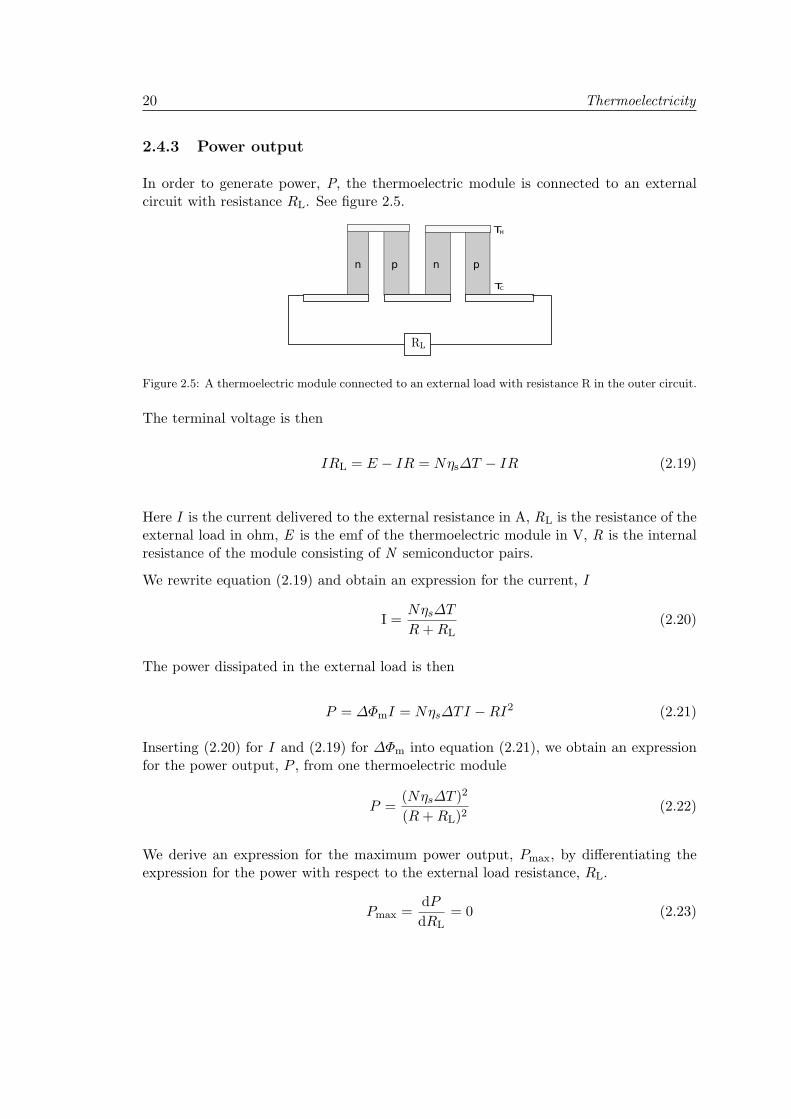
In order to generate power, P, the thermoelectric module is connected to an externalcircuit with resistance RL. See figure 2.5.
n p n p
TH
TC
Figure 2.5: A thermoelectric module connected to an external load with resistance R in the outer circuit.
The terminal voltage is then
IRL = E − IR = Nηs∆T − IR (2.19)
Here I is the current delivered to the external resistance in A, RL is the resistance of theexternal load in ohm, E is the emf of the thermoelectric module in V, R is the internalresistance of the module consisting of N semiconductor pairs.
We rewrite equation (2.19) and obtain an expression for the current, I
I =Nηs∆T
R+RL(2.20)
The power dissipated in the external load is then
P = ∆ΦmI = Nηs∆TI −RI2 (2.21)
Inserting (2.20) for I and (2.19) for ∆Φm into equation (2.21), we obtain an expressionfor the power output, P , from one thermoelectric module
P =(Nηs∆T )2
(R+RL)2(2.22)
We derive an expression for the maximum power output, Pmax, by differentiating theexpression for the power with respect to the external load resistance, RL.
Pmax =dPdRL
= 0 (2.23)

Thermodynamics of thermoelectric devices 21
Consequently, we obtain the maximum power output, Pmax, when the load resistanceequals the total internal resistance of the module, RL = R . By inserting this result intoequation (2.21), we obtain an expression for the maximum power output:
Pmax =(NηS∆T )2
4R(2.24)
Pmax can also be referred to as the matched load power output.
2.4.4 The efficiency of a thermoelectric generator
First law efficiency
The efficiency, ηI , of a thermoelectric power generator has been defined as the ratio ofthe energy supplied to the load in the external circuit, P, and the rate of heat, Q in, intothe hot side of the thermoelectric device
ηI =P
Qin(2.25)
ηI can be referred to as the device first law efficiency. According to Harman andHonig [14], the device first law efficiency can be expressed as the product of the Carnotefficiency, ηC, and the device efficiency ηdevice.
ηI = ηCηdevice (2.26)
The thermoelectric power generator maximum efficiency can be written as
ηmax = ηCγ (2.27)
Where ηC is the Carnot efficiency defined as TH−TCTH
and γ embodies the parameters ofthe materials and is given as
γ =
√1 + ZcT − 1√
1 + ZcT + TCTH
Where T = TH+TC2 and the thermoelectric figure of merit of the thermocouple is Zc =
κη2sλ .

22 Thermoelectricity
Second law efficiency
The second law of thermodynamics states that the sum of entropy change for the system,that undergoes a change, and the surroundings is equal to or larger than zero. The sumis zero for a reversible process and equals the entropy production in a time interval, ∆t,for an irreversible process: (dSirr
dt
)∆t ≡ ∆Ssys +∆Ssurr (2.28)
We can find the total entropy production for a system by integrating the local entropyprouction, σ, over the total volume of the system
dSirr
dt=∫σdV ≥ 0 (2.29)
The second law efficiency, ηII, is a measure on how well a process operates compared tothe ideal process. For a work producing process, the second law efficiency can be definedas
ηII ≡|w||wid|
(2.30)
The difference between real work obtained and the ideal work available is defined as thelost work. The rate of lost work is
wlost = w− wid = T0dSirr
dt(2.31)
The lost work is the energy dissipated as heat to the surroundings at temperature T0
and the relation is called the Gouy-Stodola theorem [35]. It states that the lost availablework is proportional to the total entropy production for the system.
By inserting equation (2.31) into equation (2.30), we obtain
ηII = 1−T0
dSirrdt
wid(2.32)
A thermoelectric power generator is a heat engine and the maximum available work isthe carnot efficiency times the heat into the generator, wid = ηCQin. The real workobtained is the power delivered to an external load, P . Introducing this into equation(2.30), we obtain
ηII =P
ηCQin
(2.33)

Thermodynamics of thermoelectric devices 23
Entropy generation in a semiconductor thermocouple
We obtain an expression for the entropy production in one semiconductor by introducingequation (2.9) and equation (2.10) into equation (2.2)
σ = −(−λdTdx
+π
Fj)
1T 2
dT
dx+ j(− 1
T(− π
TF
dT
dx− rj))
=λ
T 2(dT
dx)2 − 1
Trj2
(2.34)
We see from this that the reversible contributions cancel and that entropy is generateddue to heat conduction and joule heat, rj2.
The total entropy production in the semiconductor thermocouple, see Figure 2.1, is
dSirr
dt= Ω
∫ l
0(λ
T 2
(dTdx
)2+
1Trj2)dx (2.35)
Where Ω is the cross-sectional area, λ is the sum of the thermal conductivity for the n-and p-semiconductor, r is the sum of the ohmic resistances for the n- and p- semicon-ductors. Contact resistances between p- and n- semiconductors have been neglected.


25
Chapter 3
Thermoelectric moduleperformance
The polarisation curves, where the module potential is plotted as a function of current,is used to describe the thermoelectric module performance. We report an experimentalsetup designed to determine the performance of a thermoelectric module exposed to atemperature difference. We use the experimental setup to determine the performance ofthe thermoelectric module TEP-1264-1.5 (Termo-Gen AB, Sweden), the module poweroutput and the module first and second law efficiencies.
The module is square-shaped of size 40 mm x 40 mm and consits of 126 semiconductorpairs based on bismuth-telluride. The semiconductor pairs are connected electricallyin series and are squeezed between two ceramic plates made of aluminium oxide. Thedevice total thickness is about 3.4 mm. A picture of the thermoelectric module is shownin Figure 3.1. A fraction of one of the ceramic plates is removed, revealing some of thethermocouples. See appendix A.2 for module specifications given by the supplier.
Figure 3.1: A picture of the thermoelectric module TEP-1264-1.5 (Termo-Gen AB, Sweden). 126 semi-conductor thermocouples based on bismuth-telluride are connected electrically in series and arrangedin between two ceramic plates of aluminium oxide. A fraction of one of the ceramic plates is removed,revealing some of the thermocouples.

26 Thermoelectric module performance
3.1 Experimental
3.1.1 Experimental setup
The experimental setup enables us to measure the module potential and current as afunction of temperature difference across the device. Figure 3.2 displays a schematicdrawing of the experimental setup. Pictures of the experimental setup are given inappendix B.1.
Figure 3.2: A schematic drawing of the experimental setup used for testing the performance of a ther-moelectric module under different temperature differences across the device. The thermoelectric moduleis kept between a heat source and heat sink aluminium plate H and C, respectively. TH and TC is theheat source and heat sink temperatures. The aluminium plate marked with H is heated by an electricplate, called heater in the figure. The heat sink is water cooled, water temperature is controlled by arefrigerated water bath. The plexiglas is a part of the heat sink system. The module is kept undercompressive load, the exact measure of the load is not known. The aluminium plate marked with 1,bolts, and the aluminium plate marked with H forms the compressive system. The module is connectedto an external load and a power supply. See text for more thourough explanation.
The thermoelectric module is kept between two aluminium plates. The aluminium platemarked with H serves as heat source and the aluminium plate marked with C serves asheat sink (see figure 3.2). The module is kept under compressive load in order to facilitateheat transfer between the module and the heat source and heat sink. In addition, a thin

Experimental 27
layer thermal paste (HTSP Electrolube) is applied at the surfaces of the module in orderto further enhance heat transfer. Keeping the module under compressive load will alsostabilize the module, which expands as the temperature increases. Four bolts (two areshown in figure 3.2) goes from the aluminium heat source and through the aluminumtop plate marked with 3. The aluminium top plate is pressed downwards by using screwnuts. In addition, springs (not shown in figure 3.2) are used in between the aluminiumtop plate and the hex screws. The springs will allow the system to expand and in thatway prevent the module from breaking as the temperature increases. An exact measureof the compressive load is not known, the screw nuts were tightened using hand force.The heat sink is a water cooled aluminium plate which is square-shaped of dimensions40 mm x 40 mm; the same dimensions as the thermoelectric module. As the heat sinkaluminium plate exactly covers the thermoelectric module it will absorb all the heatpassing through the module. The heat sink aluminium plate is 20 mm thick and awater channel is milled into the aluminium plate. A plate of plexiglas glued on top ofthe aluminium plate makes the water cooling system closed and prevents heat transferbetween the aluminium heat sink and the aluminium top plate (aluminium plate markedwith 3). The heat source aluminum plate is square-shaped, 15 cm x 15 cm, 15 mm thickand it is heated by an external heater. We applied an electric plate (Beha) for heater.Glava R© was used for isolation of the module and the heat sink. This is not shown infigure 3.2.
K-type thermocouples are used for measuring the temperatures TH and TC. H refers tothe heat source aluminium plate and C refers to the heat sink aluminium plate. Twothermocouples are inserted into holes, 1 mm in diameter, in the heat sink aluminiumplate. Measuring temperatures at two locations in the plate enables us to monitor theplate temperature distribution. Three thermocouples are inserted into holes, 1 mm indiameter, in the heat source aluminium plate. Three thermocouples allow simultaneoustemperature measurement, monitoring of plate temperature distribution and in additionexternal temperature control of TH. TH is controlled by an Eurotherm PID-controllerwhich controls the effect added to the electrical plate and hence the temperature of theheat source aluminium plate. This temperature control is not shown in figure 3.2. Inaddition, K-type thermocouples are used to measure the cooling water temperatures atthe inlet and outlet of the heat sink. This is not shown in figure 3.2. The intentionof measuring these temperatures is to estimate the heat flow through the device fromthe heating of the water. All temperatures were measured by an Agilent 34970A DataAcquisition/Switch unit and logged by Agilent BenchLink Data logger 3.
The cooling water through the heat sink was controlled by a refrigerated water bath. Avalve at the water coil (not shown in figure 3.2) makes it possible to adjust the waterflow through the heat sink. This valve is located where the cooling water reenters therefrigerated water bath. The water bath temperature set point was about 15C.
The thermoelectric module is connected to an external, electronic load (Agilent 6060B)and power supply (Agilent EE3633A). The electronic load controls the thermoelectricmodule voltage (cell potential). The power supply running potentiostatically is used to

28 Thermoelectric module performance
boost the cell potential. Separate potential probes connected to the input sense of theload allows for accurate cell voltage measurements avoiding ohmic losses in the externalcircuit. A LabView setup controlled the electronic load and power supply and loggedthe cell potential and current.
3.2 Procedure
We tested the thermoelectric module steady state performance for three temperaturedifferences across the module; ∆T = 220C, ∆T = 165C and ∆T = 105C. Thesetemperature differences were obtained by controlling the heat source temperature, TH.The three different temperature differences were obtained by setting TH at 260C, 200Cand 130C. The heat sink temperature, TC, was not controlled, but determined by thecooling water that had a constant inlet temperature, controlled by the refrigerated waterbath, and the heat flow through the module. The three test condtions are summaraizedin table 3.1
Table 3.1: Thermoelectric module performance testing conditions
condition TH (C) TC (C) ∆T ()1 260 ±2 40 ±2 220 ±32 200 ±2 35 ±2 165 ±23 130 ±1 25 ±2 105 ±2
Each experiment started by setting the heat source temperature TH, this was done byadjusting the Eurotherm PID-controller temperature set point. The system was thenleft to stabilize and was assumed to be stable when the temperatures were stable within±3C.
Polarisation curves for the thermoelectric module were obtained by keeping a constantmodule potential, ∆Φm, for thirty minutes at each potential. We changed the modulepotential in steps of 0.5 V from the open circuit potential, the module emf E, to zeromodule potential.
The cooling water volume flow, V, was determined for each experiment by measuringthe time it took to fill a 100± 0.75 mL measuring glass. We used a stop watch (Jaquet)to measure the time with accuracy of ±0.1s. The mean of five repeated measurementswas taken as the cooling water volume flow, V.
3.2.1 Module efficiency
We will estimate both the first and second law efficiencies for the thermoelectric module.To calculate the first law efficiency and the second law efficiency by equation (2.25)and equation (2.33), respectively, we must know the heat flow into the thermoelectric
Procedure 29
module, Qin, when it generates power. The heat flow into the device is difficult todetermine exactly as heat is moved by the current and joule heat is generated insidethe device when I 6= 0. Therefore, we will estimate the heat flow into the module byassuming that it equals the heat conducted through the module at zero current, Q∆T,I=0.
Qin = Q∆T,I=0 (3.1)
The heat flow through the module at zero current, Q∆T,I=0, is estimated by two differentmethods, method A and B. The efficiencies are estimated for the matched load poweroutput obtainded from measurements, that is the maximum power output Pmax.
Method A - Heating of cooling water
Method A estimates the heat flow through the module at zero current by assuming thatthe heat absorbed by the cooling water at zero current equals the heat flow through themodule. The heat absorbed by the water is calculated as
Q∆T,I=0 = V ρcp∆Tw (3.2)
where V is the cooling water volume flow, ρ is the water density, cp is the water heatcapacity and ∆Tw is the difference between the cooling water outlet temperature andinlet temperature, (Tw,o − Tw,i).
The cooling water volume flow was measured to be about the same for all three ex-periments and was measured to be 2.94 mL/s within an accuracy of ±0.02mL/s. Seeappendix B, section B.3. We assume an average cooling water temperature of 20C. Weuse the values 998 kg/m3 for ρ and 4.185 KJ/Kg K for cp, which are the values givenby Geankoplis [36] for a temperature of T = 20C. The cooling water outlet and inlettemperatures are given in appendix B, section B.2 figures B.5, B.6 and B.7 and is takenat the start of experiments, that is at t = 0.
Method B - By conduction
Method B estimates the heat flow through the module as
Q∆T,I=0 =∆T
Rth= K∆T (3.3)
where ∆T = TH − TC is the temperature difference across the module in K, Rth isthe total thermal resistance of the module module in K/W and K is the module totalthermal conductivity in W/K. The relation between the total thermal conductivity, K,and the specific thermal conductivty λ is K = λ A
dx . A is the crossectional area of thedevice and dx is the thickness.
We measured K by the apparatus reported by Burheim et al [37]. The apparatus isdesigned for circular samples, 21 mm in diameter. Therefore, we cut out a circular

30 Thermoelectric module performance
sample 21 mm in diameter of the square shaped thermoelectric module. The totalthermal conductivity was measured to be K = 0.45 ± 0.05 W/K. This total thermalconductivity includes the thermal paste applied to each side of the thermoelectric moduleand is valid for the module dimensions A = 16 cm2 and dx = 3.4 mm.
Figure 3.3 illustrates the thermal resistance network that the measured total thermalconductivity is valid for. It includes the thermal paste, applied to the surfaces at bothsides of the module in order to enhance heat transfer between the heat source, moduleand heat sink, and the thermoelectric module.
Figure 3.3: Thermal resistance network illustrating what the measured thermoelectric module totalthermal conductivity, K, include. TP is the thermal paste applied the surface at each side of the modulein order to enhance the heat transfer.

Results 31
3.3 Results
3.3.1 Module potential
Figure 3.4 displays the module potential, ∆Φm, plotted as a function of current, I, forthe three experimental conditions ∆T = 220C, ∆T = 165C and ∆T = 105C. ∆T isthe temperature difference across the thermoelectric module, (TH − TC).
Figure 3.4: The thermoelectric module TEP-1264-1.5 potential, ∆Φm, as a function of current, I. ∆T isthe temperature difference across the module, (TH − TC).

32 Thermoelectric module performance
From equation (2.18) we have that the module potential equals the module emf, Nηs∆T ,when I = 0 and is lowered by a factor RI when I 6= 0. We find the module emf fromthe y-axis intersections and the internal resistance R of the module from the line slopes,these are given in table 3.2.
Table 3.2: The thermoelectric module emf, Nηs∆T , internal resistance R and corresponding temperaturedifference across the device, ∆T = (TH − TC).
∆T (C) Nηs∆T (V) R (ohm)105 3.2 ±0.1 2.54 ±0.02165 5.4 ±0.1 2.74 ±0.02220 6.8 ±0.1 2.88 ±0.02
Results 33
Seebeck coefficient
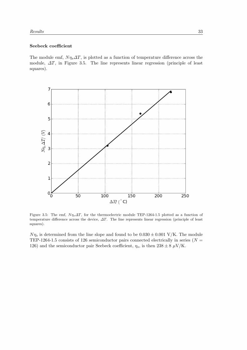
The module emf, Nηs∆T , is plotted as a function of temperature difference across themodule, ∆T , in Figure 3.5. The line represents linear regression (principle of leastsquares).
Figure 3.5: The emf, Nηs∆T , for the thermoelectric module TEP-1264-1.5 plotted as a function oftemperature difference across the device, ∆T . The line represents linear regression (principle of leastsquares).
Nηs is determined from the line slope and found to be 0.030± 0.001 V/K. The moduleTEP-1264-1.5 consists of 126 semiconductor pairs connected electrically in series (N =126) and the semiconductor pair Seebeck coefficient, ηs, is then 238± 8 µV/K.

34 Thermoelectric module performance
3.3.2 Module power output
Figure 3.6 displays the module power output, P , as calculated by equation (2.21) andplotted as a function of current I. Triangles, dots and squares represent ∆T = 220 C,165 C and 105 C, respectively. ∆T is the temperature difference across the module,(TH − TC).
Figure 3.6: The power output, P , for the thermoelectric module TEP-1264-1.5, calculated by equation(2.21) and plotted as a function of current, I
Results 35
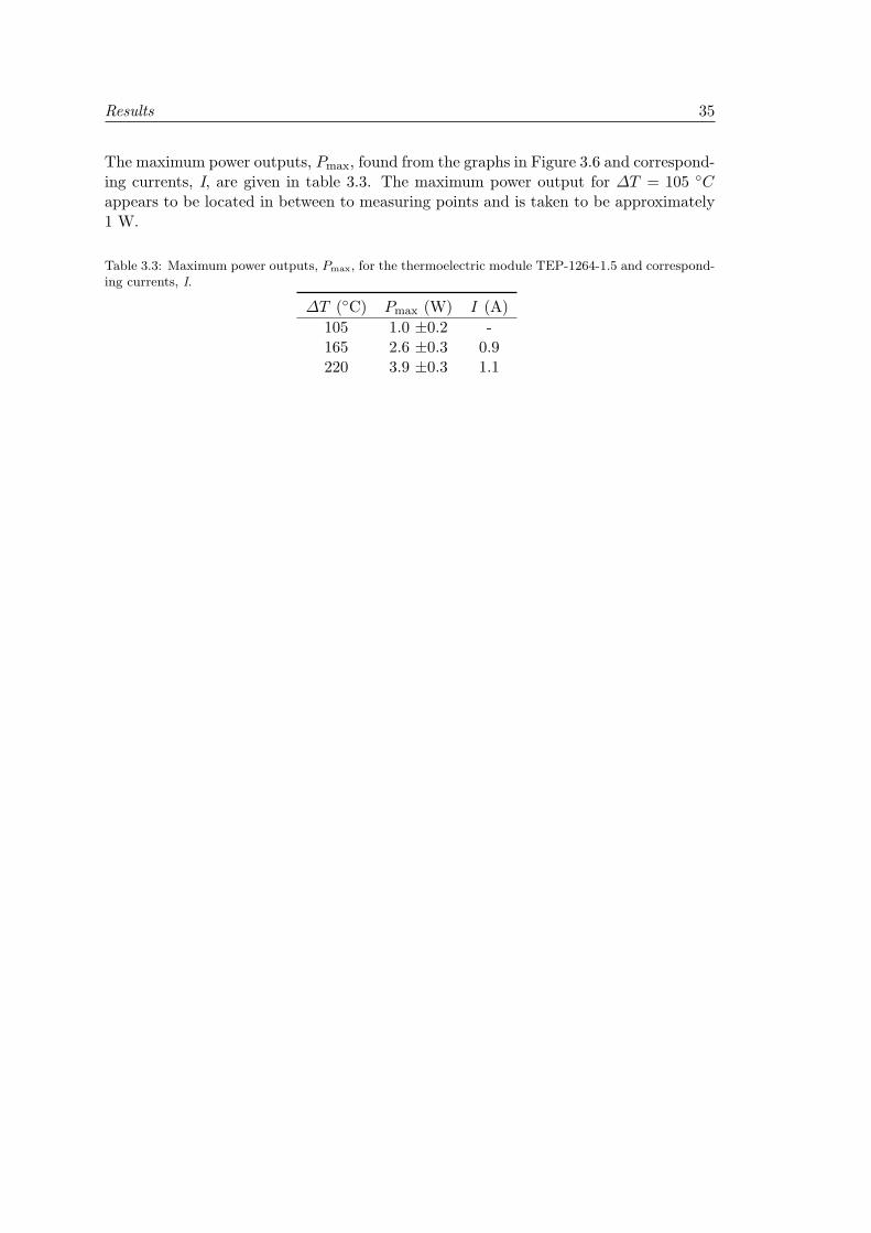
The maximum power outputs, Pmax, found from the graphs in Figure 3.6 and correspond-ing currents, I, are given in table 3.3. The maximum power output for ∆T = 105 Cappears to be located in between to measuring points and is taken to be approximately1 W.
Table 3.3: Maximum power outputs, Pmax, for the thermoelectric module TEP-1264-1.5 and correspond-ing currents, I.
∆T (C) Pmax (W) I (A)105 1.0 ±0.2 -165 2.6 ±0.3 0.9220 3.9 ±0.3 1.1
36 Thermoelectric module performance
3.3.3 Module efficiency
The heat flow into the module has been estimated by two different methods, A andB, described in section 3.2.1. Figure 3.7 displays a plot of the first and second lawefficiencies calculated by equation (2.25) and equation (2.33), respectively, and plottedas functions of temperature difference across the device, ∆T = (TH−TC). The efficienciesare calculated for the measured module maximum power output, Pmax, given in table3.3, section 3.3.2. Triangles and dots represent the calculated efficiencies when the heatflow into the module is estimated by the methods A and B, respectively. Black and redrepresent the first and second law efficiency, respectively.
Figure 3.7: The module first and second law efficiencies, ηI(black) and ηII(red), given in per cent andplotted as a function of the temperature difference across the module, ∆T . Triangles and dots representthe calculated efficiencies when the heat flow into the module is estimated by the methods A and B,respectively. Method A and B are described in section 3.2.1.

Results 37
The discrepancy between the efficiencies estimated by method A and B expresses theuncertainty in the estimated efficiencies, and will be discussed in chapter 6, section 6.1.3.


39
Chapter 4
Calorimetric study of athermoelectric device operatingin Pelitier mode
We determine the lost work in the thermoelectric module TEP-1264-1.5 (Termo-GenAB, Sweden) operating in the Peltier mode, by measure the heat deliverd by the deviceto a calorimeter. The Peltier mode is when a voltage is added to the device so that acurrent moves through the device and the device moves heat from one side to the otherside. Details for the thermoelectric device are given in the start of the previous chapterand in appendix A.2.
4.1 Experimental
4.1.1 Apparatus and experimental setup
We have used the same calorimeter as was reported by Burheim et al. [38], designedfor measuring the heat production of a fuel cell. Small modifications of the originalapparatus were necessary in order to measure the heat production of a thermoelectricdevice operating in the peltier mode. The calorimeter is constructed as a cylinder withinsulated walls so that heat transfer occurs in the axial directions. Figure 4.1 is a sketchdisplaying a cross section through the axis of the cylinder. Pictures of the calorimeterare given in appendix C, section C.1.
The calorimeter consists of two symmetrical parts, the thermoelectric device is squeezedin between the two parts. It is constructed out of four materials; aluminium, copper,steel (ss316) and PEEK (Poly Ether Ether Ketone). Two aluminium plates, 10 mmthick, are placed at the center of the apparatus. The side of the aluminum plate facing

40 Calorimetric study of a thermoelectric device operating in Pelitier mode
Figure 4.1: A sketch of the cross section through the axis of the cylindrical calorimeter. The calorimeterconsist of two symmetrical parts, the thermoelectric device is squeezed in between. TH,1, TC,1,TH,0 andTC,0 are temperatures. H refers to the left hand side of the calorimeter and C refers to the right handside of the calorimeter. 1 refers to the aluminium plates next to the thermoelectric device, 0 refers tothe copper end plates. U is the voltage applied to the thermoelectric device. See text for explanation.
outwards is disk-shaped with a diameter of 40 mm. The side facing into the center issquare-shaped, 40 mm x 40 mm; the same dimensions as the thermoelectric device. Theoriginal calorimeter was designed for disk-shaped fuel cells, and the aluminium platesmake it possible to do calorimetric study of a square shaped device. As the aluminiumplates exactly cover the square shaped device, will the heat generated by the devicebe catched by the aluminium plates. Internal heaters are placed next to the aluminiumplates. The internal heaters consists of two copper disks and a 10 Ω resistive heating wireplaced into a channel in one of the copper disks. Steel cylinders are placed next to theheaters with the purpose of thermally insulating the end plates from the heaters so that itis possible to maintain a substantial thermal gradient across each side of the calorimeter,from the aluminium plate to the end plate. The end plates are made of copper and arecooled down and kept at constant temperature by circulating cold water through copperpipes which are soldered on to the end plates. PEEK is used for constructional reasonsand because it is a good thermal and electrical insulator. Expanded polyester was usedfor isolating the part of the calorimeter not covered by the PEEK layer, i.e. parts of thealuminum plates and the thermoelectric device. Expanded polyester was also used forisolation of the cylinder in figure 4.1, the expanded polyester isolation is not shown inthe figure.
K-type thermocouples are used for measuring the temperatures TH,1, TC,1,TH,0 and TC,0.H refers to the left hand side of the calorimeter and C refers to the right hand side of thecalorimeter. 1 refers to the aluminium plates next to the thermoelectric device, 0 refersto the copper end plates. Two thermocouples are inserted into holes, 1 mm in diameter,

Experimental 41
in the aluminium plates, allowing simultaneous temperature measurement and externaltemperature control of TH,1 and TC,1. The temperatures are controlled by EurothermPID-controllers, which control the amount of heat added to the internal heaters andhence the aluminium plates temperatures. One thermocouple is taped on to each copperend plate. In addition the temperature of the heaters is measured by thermocouplesinserted into holes of 0.7 mm diameter in each heater, this is not shown in figure 4.1.
An Agilent EE3633A power supply is used to apply a voltage to the thermoelectric device.The power supply is connected to the thermoelectric device so that heat is moved fromthe right hand side to the left hand side when applying a voltage to the device AnAgilent 4338B High Frequency Ohmmeter is used to measure the ohmic resistance of thethermoelectric device. All temperatures, heat added to the heaters, current through thedevice and applied voltage was recorded by a LabView set up.
The power supplied to the heaters, Qadd,H and Qadd,C, was controlled by the EurothermPID-controllers. The cooling water to the copper end plates was controlled by a refrig-erated water bath, and was kept at approximately 10 C.

42 Calorimetric study of a thermoelectric device operating in Pelitier mode
4.1.2 Procedure
We performed three types of experiments. In experiment type I, we determined theresistance of the device as a function of device temperature. Both in experiments oftype II and type III we determined the heat generated by the device, but under differentconditions. In experiments of type II, we changed the voltage applied to the device.In experiments of type III, we kept the current constant and changed the temperaturedifference across the device. Table 4.1 summarizes the types of experiments conducted.
Table 4.1: Types of experiments conducted in the calorimeter.
ExperimentI The device internal resistance, R, is measured as a function
of device average temperature, 12(TH,1 + TC,1).
II The voltage, U, applied to the device is varied stepwise andthe heat delivered by the device to the calorimeter is deter-mined.
III The temperature difference across the device, (TH,1-TC,1), isincreased stepwise, the current, I, is kept constant and theheat delivered by the device to the calorimeter is determined.
Experiment type IWe measured the internal resistance, R, of the thermolectric device as a function ofdevice temperature. The internal resistance was measured by the Agilent 4338B HighFrequency Ohmmeter. The device temperature was set by manually controlling thealuminium plate temperature at the left and right side of the device, TH,1 and TC,1.This was done by changing the Eurotherm PID-controllers set point temperatures. Thetemperatures were kept approximately equal and the device temperature was taken asthe average of TH,1 and TC,1.
We started the experiment at TH,1 and TC,1 of 22 ±1C and raised the temperaturesby 5 ±1C every ten minutes. The end point temperatures were about 55 ±1C. Thetemperatures, TH,1 and TC,1, and the resistance, R, were logged by the LabView setupevery three seconds.
Experiment type IIWe determined the heat delivered by the thermoelectric device to the calorimeter as afunction of applied voltage, U. We changed the voltage stepwise in the range from U =0.0 V up to U = 4.0 V. Each experiment was started at U = 0 and the voltage was keptat one level at least one hour in order to have stable measurements. The Eurotherm PID-controllers temperature set points were 50 C for both TH,1 and TC,1. The temperaturedifference across the device, ∆T = (TH − TC), was not zero or constant as the voltagewas increased during the experiments. The reason for this was that the Eurotherm-PIDcontrollers set a limit on the power delivered to the heaters.

Experimental 43
All temperatures (TH,1, TC,1, TH,0 and TC,0), power deliverd to the heaters (Qadd,H andQadd,C), applied voltage (U ) and current through the device (I ) were recorded by theLabView set up every six seconds.
Experiment type IIIWe determined the heat delivered by the thermoelectric device as a function of thetemperature difference, ∆T = TH,1 - TC,1, across the device. Each experiment wasstarted at a TH,1
∼= TC,1 of approximately 50 C and the current was kept constant at1.00±0.05A throughout the experiments. The current was kept constant by adjusting thevoltage difference, U, across the device. The temperature difference, ∆T , was increasedby lowering TC,1. This was done by lowering the set point temperature for the EurothermPID-controller controlling TC,1. The ∆T was kept at one level about an hour in order tohave stable measurements. All temperatures (TH,1, TC,1, TH,0 and TC,0), power deliverdto the heaters (Qadd,H and Qadd,C), impressed voltage (U ) and current through thedevice (I ) were recorded by the LabView set up every six seconds.

44 Calorimetric study of a thermoelectric device operating in Pelitier mode
Data analysis
Figure 4.2 is a schematic drawing, explaining the principle of the calorimeter, see figure4.1, used for determining the heat delivered by the thermoelectric device, operating inthe Peltier mode, to the surroundings, i.e. the calorimeter. The direction of current isso that heat is moved from the right hand side to left hand side of the device.
Figure 4.2: A schematic drawing explaining the principle of the calorimter used for determining theheat production of a thermoelectric device. The thermoelectric device is kept in between the two partsof the calorimeter which are mirror symmetric. Qadd,H and Qadd,C is heat added to each part of thecalorimeter. Qflow,H and Qflow,C is the heat flowing out of the calorimeter. H and C refers to the left andright hand side of the thermoelectric device, respectively. Q is the heat supplied to the calorimeter by thethermoelectric device. TH and TC is the temperature in the aluminium plates next to the thermoelectricdevice, at the two sides.
The calorimeter consists of two symmetrical parts, the thermoelectric device is squeezedin between. Heat is added to the heaters at each side of the calorimeter, and heat flowsout of the calorimeter at each side, see figure 4.2. As the thermoelectric device is square-shaped, while the calorimeter is designed for cylindrical units we will operate with totalquantities and not fluxes.
In order to use the thermoelectric device as a heat pump we must provide work to theelement. This work is the effect, P , added to the device and equals
P = UI = Nηs∆TI +RI2 =Nπ
T∆TI +RI2 (4.1)
Where N is the number of semiconductor pair in the device, ηs is the Seebeck coefficientdefined in section 2.4.2, ∆T is the temperature difference across the device (TH−TC). Ris the device internal resistance, π is the peltier coefficient defined in section 2.4.1 and Tis the device average temperature, taken as the average of the calorimeter temperatures

Experimental 45
TH and TC, 0.5(TH + TC). When TH > TC, the applied work, P , must overcome thepotential induced by the temperature difference pluss the ohmic resistance.
The first law of thermodynamics gives the change in internal energy of the thermoelectricdevice. At steady state conditions the change in internal energy is zero and we obtain
∆U = Q + P = 0⇒ P = −Q (4.2)
From this, we have that the effect added to the thermoelectric device equals the heatdelivered by the device to the surroundings, i.e. the calorimeter. The energy balance forthe calorimeter given in Figure 4.2 is
Q = P = (Qflow,H − Qadd,H) + (Qflow,C − Qadd,C)
= QH + QC
(4.3)
Where H and C denotes left and right of the calorimeter, respectively. Qflow,H and Qflow,C
is heat flowing out of the calorimeter, Qadd,H and Qadd,C is heat added to the calorimeterat the two sides, see figure 4.2.
Determining the lost work assuming TH = TC
The rate of lost work of a process relative to the surroundings equals the total entropyproduction times the surroundings temperature, see equation (2.31). When TH = TC
we have that the heat delivered by the thermoelectric device to the calorimeter, Q,equals the rate of lost work of the thermoelectric device given by equation (4.3). Thetotal entropy production is found by integrating the local entropy production over thevolume of the device, see equation (2.29). We introduce equation (2.34) for the localentropyproduction and obtain
Q = TdSirr
dt
= TA
∫ l
0
( λ′T 2
(dTdx
)2− π
FT 2
dT
dxj +
π
FT 2
dT
dxj +
1Tr′j2)dx
= TA
∫ l
0
( λ′T 2
(dTdx
)2− π
F
dlnT
Tj
1dx
+π
F
dlnT
Tj +
1Tr′j2)dx
= K∆T 2
T+RI2
(4.4)
Where λ′ is the combined thermal conductivity of the device, r′ is the device combinedresistivity. K is the total thermal conductivity of the thermoelectric device in WK−1, R

46 Calorimetric study of a thermoelectric device operating in Pelitier mode
is the device total internal resistance in ohm. A is the device cross sectional area in m2
and l is the device thickness in m. T is the average device temperature. The reversiblecontributions cancels and work is lost due to heat conduction and Joule heating. Thesurroundings in this case is the calorimeter, and the surroundings temperature will bethe average temperature of the two sides of the calorimeter.
T ∼= T =12
(TH,1 + TC,1
)(4.5)
Determining the lost work when TH 6= TC
The total entropy production equals the rate of entropy flowing out minus the rate ofentropy flowing and in when TH 6= TC and is
dSirrdt
= A
∫ l
0
( λ′T 2
(dTdx
)2+
1Tr′j2)dx
= K∆T 2
T2 +1TRI2
= (Qflow,H
TH+
Qflow,C
TC)− (
Qadd,H
T+
Qadd,C
T)
= (Qflow,H
TH−
Qadd,H
T) + (
Qflow,C
TC−
Qadd,C
T)
(4.6)
The lost work is then found by mulitply the total entropy production calculated byequation (4.6) by the surroundings temperature given in equation (4.5).
We calculate also the absolute value for the heat flowing out of the calorimeter at thetwo sides, Qflow,j,as the temperature difference over the thermal resistance,
Qflow,j =Tj,1 − Tj,0
Rj(4.7)
j is either H or C. T j,1 is the temperature of the aluminium plates next to the ther-moelectric device. T j,0 is the temperatures of the copper end plates. Rj is the thermalresistance of side j.
At U = 0 and ∆T = 0, there is no flux of current or heat through the device andconsequently no heat generated by the thermoelectric module. Then, the heat addedto the internal heaters equals the heat flowing out of the calorimeter. At U = 0, wecalculate the thermal resistances for the two sides from equation (4.7). We assume thatthe thermal resistances calculated at U = 0 and ∆T = 0 is constant throughout theexperiment.
Experimental 47
Determining the Seebeck coefficient
QH and QC are the differences between the heat flowing out of the calorimeter at eachside and the heat added, see equation (4.3). From equation (4.4) and assuming that halfof the heat supplied by the thermoelectric device to the calorimeter enter each side ofthe calorimeter we obtaint
QH =π
F∆(lnT )I +
12
Q (4.8)
QC = − πF∆(lnT )I +
12
Q (4.9)
Where πF∆lnT I is the heat moved reversibly by the current. The difference between QH
and QC is
QH − QC = 2π
F∆ lnTI (4.10)
Where 12(QH− QC) is interpreted as the heat moved reversibly by the device. A plot of
12(QH − QC) versus current should give a straight line. The Seebeck coefficient for thesemiconductors in the device can be found from the slope of the line and by using therelation between the Seebeck and Peltier coefficient given in equation (2.16).

48 Calorimetric study of a thermoelectric device operating in Pelitier mode
4.2 Results
4.2.1 Experiment type I
Figure 4.3 displays the measured device internal resistance, R, plottet as a function ofdevice average temperature, T = TH,1+TC,1
2 in units of C.
Figure 4.3: The total ohmic resistance, R, in ohm of the thermoelectric device TEP-1265-1.5 as measuredby the Agilent 4338B High Frequency Ohmmeter plotted as a function of the device average temperature,T in units of C.
Linear regression (principles of least squares) gives this expression for the device totalohmic resistance:
R = 1.403 + 0.00758 ∗ T (4.11)
The ohmic resistance is given in units of ohm with a standard error of ± 0.01 ohm, thetemperature T is in units of C.

Results 49
4.2.2 Experiment type II
The results given in this section is based on data from three experiments, raw data aregiven in appendix C, section C.2.1. There is a temperature difference across the device,∆T , when I 6= 0, see figure C.7.
Determining the lost work, assuming TH = TC
The lost work of the thermoelectric device TEP 1264-1.5 is determined as the heatdelivered by the device to the calorimeter, Q, caculated by equation (4.3). Q and theeffect added to the device, P = UI, are plotted as functions of current, I in Figure 4.4.
Figure 4.4: The lost work of the thermoelectric device TEP-1264-1.5, Q , and the effect added to thedevice, P = UI, as a function of current, I. ∆T 6= 0 when I 6= 0, ∆T is the temperature difference acrossthe device.
The uncertainty in Q is due to fluctuations in Qadd,H and Qadd,C and error in thecalculated heat flows Qflow,H and Qflow,C. The uncertainty in P is due to error in currentmeasurements.

50 Calorimetric study of a thermoelectric device operating in Pelitier mode
Determining the lost work when TH 6= TC
The device total entropy production, dSirrdt , is calculated by equation (4.6) and multi-
plied by the calorimeter average temperature T. The result is plotted together with Q,calculated by equation (4.3) as functions of current I.
Figure 4.5: The device lost work, T dSirrdt
, determined by equation (4.6), the lost work Q calculated byequation (4.3) plotted as functions of current, I. ∆T 6= 0 as I 6= 0, ∆T is the temperature differenceacross the device.

Results 51
Effect and Joule heat
Figure 4.6 displays a plot of the effect added to the device, P = UI, and the joule heatRI2 as functions of current I. The device internal resistance, R, is taken from figure 4.3.
Figure 4.6: The effect P = UI added to the device TEP-1264-1.5 and the joule heat, RI2 generated bythe device TEP-1264-1.5 as a function of current I. R is taken from figure 4.3. ∆T 6= 0 as I 6= 0, ∆T isthe temperature difference across the device.
The uncertainty in both P and RI2 stem from error in current measurements.
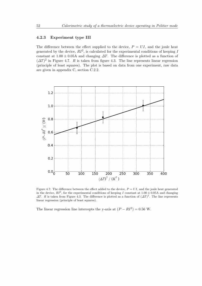
52 Calorimetric study of a thermoelectric device operating in Pelitier mode
4.2.3 Experiment type III
The difference between the effect supplied to the device, P = UI, and the joule heatgenerated by the device, RI2, is calculated for the experimental conditions of keeping Iconstant at 1.00 ± 0.05A and changing ∆T . The difference is plotted as a function of(∆T )2 in Figure 4.7. R is taken from figure 4.3. The line represents linear regression(principle of least squares). The plot is based on data from one experiment, raw dataare given in appendix C, section C.2.2.
Figure 4.7: The difference between the effect added to the device, P = UI, and the joule heat generatedin the device, RI2, for the experimental conditions of keeping I constant at 1.00± 0.05A and changing∆T . R is taken from Figure 4.3. The difference is plotted as a function of (∆T )2. The line representslinear regression (principle of least squares).
The linear regression line intercepts the y-axis at (P −RI2) = 0.56 W.

Results 53
4.2.4 Seebeck coefficient
The measurement data for experiment of type II are evaluated by equation (4.10) andmulitiplied by 0.5. The results are plotted as a function of current in Figure 4.8 and isbased on data from three experiments. Raw data are given in appendix C, section C.2.1
Figure 4.8: The difference between QH and QC multiplied by 0.5 and plotted versus current, I. The linerepresents linear regression (principle of least squares) on the points from current of I = 0.8 and above.
The line is linear regression on the points for I = 0.8 A and higher. The line slope is foundto be 5.32± 0.03 J/C. According to equation (4.10), the line slope can be interpreted asπF∆(lnT ). The Seebeck coefficient for the semiconductor pairs is determined using therelation between the Seebeck and Peltier coefficents given in equation (2.16), dividingthe line slope value by the number of semiconductor pairs connected electrically in series,N = 126, and by using the averages of ∆(lnT ) and device average temperatures, T, forI = 0.8 A and higher. The Seebeck coefficient is then found to be ηs = 3.82±0.02 mV/K.


55
Chapter 5
Thermoelectric power generatordemonstration unit
The design of the demonstration unit is a result of cooperation with Termo-Gen AB(Sweden), represented by Lennart Holmgren, who also built the unit. The unit will bemounted on a stand with wheels so that it easily can be moved around in the castingarea and be handled by one person. A description of the thermoelectric power generatorand the stand is given in section 5.1. The demonstration unit was delivered severalweeks behind schedule and there was no time for testing. A tentative testing procedureis briefly outlined in section 5.2.
5.1 Demonstration unit
Description of thermoelectric power generator
Based on the calculated heat flux of of 19 kW into the wall mounted in the casting area(see section 1.1.2), the thermoelectric power generator has been desgined to withstand aheat flux of 22.5− 25 kW/m2 into the hot side. It has been estimated to provide 100 Wgross, even at a heat flux of 15 kW/m2.
Figure 5.1 shows a 3D drawing of the thermoelectric power generator. It is square-shaped (0.5 m x 0.5 m) and consists of a heat block, 36 square-shaped (40 mm x 40 mm)thermoelectric modules (TEP-1264-1.5) and six heat sinks.
The heat block (blue details in figure 5.1) will be directed towards the liquid silicon andbe heated by thermal radiation. It consists of 36 square-shaped units, 80 mm x 80 mm,made of 10 mm thick aluminum plates. The planar front side of the units will be facingtowards the liquid silicon and the thermoelectric modules will be attached to the backside of the units. The back side is bevelled so that the heat flow will be directed into

56 Thermoelectric power generator demonstration unit
Figure 5.1: A 3D drawing of the thermoelectric power generator demonstration unit. The blue detailsis the heat block that will be facing towards the heat source. The thermoelectric modules are wedgedin between the heat block and the water cooled heat sinks by bolts running through the heat block andthe U-beam. See text for more thoroughly explanation.

Demonstration unit 57
the modules. Figure 5.2 is a picture showing both the front (unit at right hand sidein picture) and back (unit at left hand side in the picture) of a unit in the heat block.There is a gap between the heat block units as they will expand as temperature increase.
Figure 5.2: Picture of two units in the heat block system, showing both sides of the heat block units.The unit to the right shows the planar front that will be directed towards the heat source. The unit tothe left shows the bevelled back side to which the thermoelectric device will be attached.
The thermoelectric modules are wedged in between the heat block units and the heatsinks by spring-loaded bolts running through the heat block units and the U-beam. Usingspring-loaded bolts will allow the system to expand and in that way prevent the modulefrom breaking as temperature increase. The 36 modules are connected electrically inseries of six and six groups are connected in parallel. This initial coupling is adapted toa 12 V system and will yield a voltage output of approximately 14 V . The voltage ouputdepends the temperature difference across the generator, i.e. upon the heat flux into thegenerator, not known exactly, and the cooling capacity. If cooling works well and theheat flux is larger than assumed, the voltage output will be too high for a 12 V system.Therefore, the modules are connected so that they can be rearranged into series of fourmodules and nine groups connected in parallel, in that way will the voltage output belowered. The six heat sinks are made of aluminium and water cooled. The water willenter and exit the heat sink at the locations indicated in figure 5.1 and flow in a zigzagpattern from the inlet to the outlet. A cooling unit of the type intended for use in carscontrols the cooling water flow and temperature. An external battery will be used torun this cooling unit. The cooling water voulme flow will be measured by a flow sensor.
K-type thermocouples are included at three locations at the diagonal of the heat block tofacilitate the survey of temperature distribution in the heat block. K-type thermocouplesare also included in the heat sink so that the temperature difference across the generatorcan be measured. In addition, knowing the hot side and cold side of the thermoelectricmodules is important as they can be damaged if exposed to too high temperatures. K-type thermocouples are also included at the cooling water inlet and outlet so that theheat flow through the generator can be estimated from cooling water volume flow andtemperature increase from inlet to outlet. From the heat flow through the module can

58 Thermoelectric power generator demonstration unit
the generator efficiency be estimated.
Description of stand
Figure 5.3 shows a picture of the stand that the thermoelectric power generator will bemounted on. The green watering can illustrates the thermoelectric power generator.
Figure 5.3: A picture of the stand that the thermoelectric power generator will be mounted on. The greenwatering can illustrates the thermoelectric power generator. See text for more thorough explanation.
The stand is made of aluminium profiles which make it possible to modify it if necessary.A part of the stand is moveable and can be raised and lowered by a winch, the maximumheight is 250 cm above the floor. The generator is attached to the stand in a way whichmake it possible to alter the angle of the generator and the heat flux into it be optimized.The battery for the cooling unit will be placed at the bottom of the stand together withequipment for measuring and logging of voltage output, current, temperatures and watervolume flow.
5.2 Testing procedure
The thermoelectric power generator will be tested before taking it to the casting area atthe silicon plant. In the pre-test, radiant heaters will be used as a heat source in orderto simulate the liquid silicon and it will be performed in a clean envrionment. A purposeof this pre-testing is to investigate how the performance of the generator is affected bythe dusty environment at the plant and also to learn using the generator.
The amount of thermal radiation to the surroundings differs between the individualcastings and varies as the process advances. Therefore, the testing at the plant shouldtake place over a longer period of time in order to investigate how the generator isaffected by the cyclic heating.

59
Chapter 6
Discussion
Section 6.1 discusses the results obtained from the performance testing and improvementsin the experimental set up. The results from the calorimetric study are discussed insection 6.2. Suggestions for future work are given in section 6.3.
6.1 Performance testing
6.1.1 Module potential
From Figure 3.4 we see that the measured module potential, ∆Φm, decreases linearlywith increasing current, I, for all three experiments. This observation is in accordancewith equation (2.18) and therefore expected. We observe that the internal resistanceof the device, given in table 3.2, increases with increasing device temperature. Thesemiconductor’s electric resistivity increases as the electrical conductivity decline byincreasing temperature, see appendix A.3. An increase in module internal resistanceis therefore expected when temperature is increased. We calculate the module internalresistance by equation (2.17), using electrical conductivity data given in appendix A.3at the average temperatures of the device, T= 0.5(TH + TC), in each experiment. Thesemiconductor dimensions are given in appendix A.1. The resistances calculated byequation (2.17) are 2.26 ohm, 2.06 ohm and 1.74 ohm for ∆T = 220C, 165C and 105C,respectively. The calculated resistances are lower than the experimentally determinedones. Contact resistance is neglected when calculating the internal resistance by equation(2.17) and may explain the discrepancy between the measured and calculated values.
We also observe that the module potential increases with increasing temperature differ-ence across the device, ∆T . We recall that the maximum module potential is the moduleemf and that the module emf increase with increasing ∆T . Thus, the the experimentalresult is in agreement with the theory.

60 Discussion
Comparing to supplier dataThe supplier gives an open circuit voltage of 8.6 V and an internal resistance of 3 ohmat the design temperatures TH = 230 C and TC = 50 C (∆T = 180C), see appendixA.2. At ∆T = 220C, the internal resistance was determined to be 2.88 ohm, which isabout the same as the internal resistance provided by the supplier, while we measuredan open circuit voltage, the emf, to be 6.8 V, that is approximately 20 % lower thanthe emf measured by the supplier. As the emf is expected to increase with increasingtemperature, this observation may indicate that the performance data given by thesupplier is incorrect and that establishing testing procedures for testing the performanceagainst the performance data provided by the supplier is important.
Seebeck coefficient
The Seebeck coefficient, ηs, for the semiconductor pairs in the thermoelectric moduleTEP-1264-1.5 is determined from the slope of the linear regression line in Figure 3.5to be 238 ± 8 µV/K. Determining the Seebeck coefficient from the slope of the linearregression line is based on the assumption that the Seebeck coefficient is constant and in-dependent of temperature. The Seebeck coefficient is related to the transported entropiesof the semiconductors through equation (2.15). The transported entropy is a functionof temperature [3] and the assumption of constant transport entropies only holds when∆T is small [39]. However, data for the Seebeck coefficients for the p- and n-type semi-conductors that constitutes the module, given in appendix A.3, yields that both theSeebeck coefficient for the p- and n-type semiconductors are about constant within thetemperature range 300K < T < 425K. The device average temperature is 350K and423K when ∆T = 105 C and ∆T = 220 C, respectively. Thus, we operate within therange of constant Seebeck coefficients. The Seebeck coefficients provided for both the p-and n- type semiconductors in appendix A.2 are positive. The transported entropies forthe n- type semiconductors is by convention negative and consequently so is the Seebeckcoefficient [14]. Assumuing that the Seebeck coefficients provided in appendix A.2 areabsolute values, we obtain a semiconductor pair Seebeck coefficient of about 435 µV/Kfor the temperature range 300K < T < 425K which is larger than the experimentallydetermined Seebeck coefficient. The exact composistions and preparation techniques ofthe semiconductors are not known to us. A material’s Seebeck coefficient is dependentupon the materials composition as well as the preparation technique [40], therefore wehave not compared the experimental determined Seebeck coefficient with values foundin literature, expect from data provided by the supplier.
When determining the Seebeck coefficient from the slope of the linear regression linewe use the temperature difference across the whole module. The emf is proportional tothe temperature difference across the semiconductor pairs, which is placed between twoceramic plates. This difference in ∆T (illustrated in Figure 6.1) may give an error in theexperimentally determined Seebeck coefficient.
Due to the uncertainty in temperature measurements, this procedure may not be suit-

Performance testing 61
Figure 6.1: A schematic drawing of thermoelectric module squeezed in between the heat source aluminiumplate and the heat sink aluminium, denoted H and C in the figure, respectively. plate in the experimentalset up given in section 3.1.1. The components marked with * are the ceramic plates, componentsmarked with # is the electrical conductor and components marked with n and p are the n- and p-type semiconductors, respectively. ∆Tin and ∆To is the internal and external temperature difference,respectively.
able to determine the exact value for the Seebeck coefficient for semiconductor pairs in athermoelectric module, but the method can provides an estimate. Further, determiningthe Seebeck coefficient using this procedure demands that the semiconductor pairs areconnected electrically in series which may not be the case for a random thermoelec-tric module. However, the proportionality factor for the emf, Nηs, can be determinedand serve as a characterisation of a module. However, more experiments with differentmodules should be done in order to further test this procedure’s validity and limitations.
6.1.2 Module power output
We recall from equation (2.21) that the thermoelectric module power output, P, is com-posed of the module emf times the current, Nηs∆TI, and the resistance times the squareof current, RI2. The power output reaches a maximum when the resistance of the exter-nal circuit, RL, equals the module internal resistance, R, as shown in section 2.4.3. FromFigure 3.6 we observe that the thermoelectric module power output increases, reaches amaximum and then decreases as the current increases, as expected. We also note thatthe power output increases as ∆T is increased. An increase in module power output as∆T increases is expected due to the increase in module emf, as discussed in the previoussection. We also observe that the location for the maximum power shifts to right byan increase in ∆T across the device. The current I equals the emf over the sum ofthe internal and external resistances (see equation (2.20)). As discussed in the previoussection both the emf and the internal resistance R increase with increasing temperaturedifference. However, the increase in internal resistance is small compared to the increase

62 Discussion
in emf. When the module internal resistance equals the load resistance, the moduledeliver the maximum power to the external load and as the emf is a stronger function oftemperature than the internal resistance, the matched load current will increase by anincrease in ∆T and we observe a shift to the right for the location of Pmax.
Comparing to supplier dataAt ∆T = 180C, the supplier gives a matched load power output Pmax = 5.9 W (seeappendix A.2), we determined a Pmax = 3.9 W for ∆T = 220C. This discrepancy isexpected due to the discrepancy between the experimentally determined emf and theemf provided by the supplier, discussed in the previous section.
6.1.3 Module efficiency
From Figure 3.7 we observe that both the first and second law efficiencies, ηI and ηII,calculated for method B are larger than ηI and ηII calculated for method A. The discrep-ancy between the efficiencies calculated for method A and B is due to the discrepancybetween the heat flow into the module, Q in, estimated by the two methods. The heatflow into the module estimated by method A is higher than the heat flow into the moduleestimated by method B. There may be several reasons for this. First, no isolation wasused between the bolts connecting the heat source aluminium plate and the aluminiumtop-plate (see figure 3.2) which may explain the discrepancy. A schematic drawing illus-trating the heat flow in the experimental set up is given in Figure 6.2, the heat flow isillustrated by the arrows in the figure.
Figure 6.2: Illustration of heat flow in the experimental set up described in chapter 3, section 3.1.1. Thered arrows illustrates the heat flow.
Second, there may be an error in the experimental determined device total thermalconductivity, K = 0.45 ± 0.05 W/K. The thermal conductivity was measured for acircular fraction of the thermoelectric device and may not be representative for thesquare-shaped device. The supplier gives a total heat flow of 140 W through the deviceat the design temperatures TH = 230 C and TH = 50 C (see appendix A.2), which yieldsa total thermal conductivity of K = 0.77 W/K. This indicates that the experimentaldetermined total thermal conductivity may be to low which contributes to the error.The set up should be improved by isolating the bolts and then compare the heat flow
Performance testing 63
estimated by the two methods in order to determine whether the measured total thermalconductivity is reliable or not.
Additionally, the heat flow into the device was estimated as the heat conducted throughthe device when I = 0. The heat into the device when I 6= 0 does not equal the heatflow through the device when I = 0. A part of the heat flowing into the device whenI 6= 0 will be converted to work. In addition, heat will be moved through the device bycurrent (Peltier effect) and heat will be generated inside the device due to Joule heating.Therefore, exact determination of the heat flow into the device when I 6= 0 is not aneasy task. One way to solve this could be to redesign the experimental set up.
From Figure 3.7 we see that the second law efficiencies calculated for both method A andB are higher than the first law efficiencies. We also observe that the second law efficiencyestimated by both methods has a maximum in ∆T = 165 C, while the first law efficiencyincreases linearly with ∆T . The discrepancy between ηI and ηII can be explained fromthe definition of the efficiencies, see equation (2.25) and equation (2.33). The first lawefficiency gives the fraction of useful energy out (the electric work, P) over the energy intothe system, Q in. The second law efficiency gives the fraction of useful energy out overthe maximum obtainable energy out. That is, ηII compares the thermoelectric moduleperformance to the ideal heat engine and thus say something about how close to reversiblethe thermoelectric device operates. The maximum work that can be obtained from aheat flow in a heat engine is wmax = wid = ηCQ in and consequently the estimated secondlaw efficiencies are higher than the first law efficiencies. The maximum observed for ηIIindicates that the degree of reversiblity of the thermoelectric module is temperaturedependent. This may be useful to know when determining the operating temperaturefor a module. The second law efficiency is useful for design purposes and in optimisingmachines and processes. The first law efficiency is useful for determining how much workyou can expect from from a given amount of heat input when the efficiency is known.
Comparing to supplier dataThe module first and second law efficiencies estimated from the data provided by thesupplier at the design temperatures (∆T = 180C, appendix A.2) are 4.2 % and 11.8%, respectively, which is larger than the first and second law efficiencies estimated bymethods A and B (see figure 3.7) for ∆T = 220C and ∆T = 165C. This discrepancybetween the efficiencies obtained from data provided by the supplier and efficienciesobtained from experiments can be explained by the fact that the module emf given bythe supplier is larger than the experimentally determined values, discussed in section6.1.1.

64 Discussion
6.2 Calorimetric studies
6.2.1 Experiment type I
From figure 4.3 we see that the measured device internal resistance, R, increases lin-early by increasing device temperature. The increase in internal resistance by increas-ing temperature corresponds to the observations from the potential measurements, dis-cussed in section 6.1.1. We have calculated the module internal resistances by equation(4.11) and for the device average temperature for the performance testing conditions of∆T = 105C, 165C and 220C. The results are given in table 6.1. We observe that thecalculated values are lower than the values determined experimentally in section 3.3.1and that the discrepancy decreases by increasing device temperature.
Table 6.1: Module internal resistances as determined from experiments in section 3.3.1, R, calculated byequation (4.11),Rc, and the deviation between them.
∆T (C) R (ohm) Rc (ohm) deviaton (%)105 2.54 1.99 21.7165 2.74 2.28 16.8220 2.88 2.54 11.8
Equation (4.11) has been obtained from measurements for a device temperature in therange from 20C up to 50C and may not be valid outside this temperature range. Thismay explain the discrepancy and the internal resistance should be measured by thisprocedure for higher device temperatures to check this.
6.2.2 Experiment type II
Determining the lost work, assuming TH = TC
From Figure 4.4 we observe a discrepancy between the heat delivered by the device tothe calorimeter, Q, calculated by equation (4.3) and the effect added to the device, P .We also see that both Q and P increases by increasing current and that the curves aresmooth ignoring Q for 0 < I < 0.6 A. This increase with increasing current is expectedfrom equations (4.1) and (4.3). At low currents, 0 < I < 0.6 A, Q is larger than P . Forcurrents from about I = 1 A and higher Q is smaller than P . From equation (4.3) weexpect that Q equals P . That Q is larger than P indicates that we operate outside thevalid measuring range for the calorimeter. At higher currents, the observed discrepancyindicates that there is a heat leakage in the system. This heat leakage may be dueto Joule heating in the electric cables into the thermoelectric device. The cables arelocated outside the calorimeter so that heat generated in these will not be absorbed inthe calorimeter. This explanation is further strengthened by the fact that the discrepancy

Calorimetric studies 65
increase by increasing current. In future experiments the length of the cables should beminimized and measurements be performed in the valid measuring range.
Measuring heat is difficult and we observe that the uncertainty in Q is relatively largecompared to the uncertainty in P . This indicates that the method may be best for aqualitatively determination of the lost work.
The calorimeter is designed to be isothermal, but isothermal conditons was not the casewhen I 6= 0 as shown in figure C.7, appendix C.2. When I 6= 0 we had the condition ofTH > TC and determining the device lost work as Q will only be an approach.
Determining the lost work when TH 6= TC
From Figure 4.5 we observe that the lost work calculated by equation (4.6) and multipliedby the average calorimeter temperature, T dSirr
dt , equals Q calculated by equation (4.3).This indicate that determining the lost work of the thermoelectric device as Q is anacceptable approach.
Effect and Joule heat
From Figure 4.6 we see that both the effect added to the device, P , and the Joule heat,RI2, generated in the device increase by increasing current as is expected. We observea discrepancy between P and RI2 for I > 0.4 A that increases by increasing current.We recall from equation (4.3) that P equals the heat supplied by the device to thecalorimeter and that work is lost both due to heat conduction and Joule heating. Fromequation (4.3) we have that the work lost due to heat conduction is proportional tothe square of the temperature difference across the device.As discussed previously, theconditions were not isothermal in the calorimeter when I 6= 0. In fact, the temperaturedifference ∆T = (TH − TC) increased by increasing current. Therefore, we expect thatthe observed discrepancy is due to heat conduction.

66 Discussion
6.2.3 Experiment type III
From Figure 4.7 we observe that the difference between the effect added to the device,P , and the Joule heat, RI2, increases by increasing temperature difference across thedevice, ∆T . As I is kept constant during the experiment, the observed effect is due toheat conduction. The line representing the linear regression intercepts the y-axis where(P - RI2) = 0.54 W. This indicates that the lost work is not only due to Joule heatwhen ∆T = 0, or said in another way; ∆T cannot be zero. We recall from section 2.4.1that heat is transported reversibly by current, as a consequense of this there will be atemperature difference across the device when I 6= 0. That is, the internal temperaturedifference, ∆Ti , is not necessarily zero when the external temperature difference, ∆To,equals zero. This is illustrated in figure 6.3. ∆To and ∆Ti are explained in section 6.1.1.
Figure 6.3: The internal temperature difference, ∆Tin, plotted as the external temperaturedifference,∆To, when I 6= 0.
As work is lost both due to heat conduction and Joule heating the thermal conductivityand the internal resistance the semiconductor pairs that constitute a thermoelectricmodule should be minized in order to reduce the lost work. As discussed previously maythe internal and external difference across a module be different, therefore the thermalconductivity of the ceramic plates should be as high as possible.
6.2.4 Seebeck coefficient
The Seebeck coefficient for the semiconductor pairs in the thermoelectric device is bythe calorimetric method determined to be 3.82 ± 0.02 mV/K. This value is an order ofmagnitude larger than the Seebeck coefficient found from module potential measurementsin section 3.3.1. The value found from potential measurements was of the same orderof magnitude as the Seebeck coefficient estimated from semiconductor data providedby the supplier (see section 6.1.1) and is therefore assumed to be more reasonable.This indicates that the Seebeck coefficient determined by the calorimetric method isoverestimated and that the model used for find the Seebeck coefficient (equation (4.8)and (4.9)) may be too rough or incorrect it should therefore be further improved to seeif the two methods can estimate corresponding values for the Seebeck coefficient. The
Further work 67
measured heat is determined within relatively large uncertainty and to exact measureheat is difficult. Therefore, Seebeck coefficient should rather be determined from thepotential measurements than by the calorimeteric method.
As discussed in section 6.2.2 measurement for 0 < I < 0.6 is most probably outside thevalid measurement range for the calorimeter and is therefore omitted from the linearregression represented by the line in figure 4.8.
6.3 Further work
The thermoelectric power generator demonstration unit reported in chapter 5 should betested as outlined in the tentative testing procedure (section 5.2). Testing the generatorunder real conditions at the silicon plant will be necessary in order to determine whetherthermoelectric devices are a realistic measure for recovering of thermal radiation fromthe liquid silicon.
Further, the measures proposed to improve the testing and characterisations proceduresshould be performed in order to develop more robust and precise procedures.
Other methods for the direct conversion of heat into electricity should be investigated.For example, Hemmes et al [41] propose a fuel cell reactor for cogeneration of chemicalsand electric power. This fuel cell reactor has the ability of converting the heat of reactiondirectly into electric power. If the reaction exhibit a positive entropy change couldan additional amount of heat, waste heat, be converted to electric energy. So calledthermogalvanic cells represent another possibility for the direct conversion of heat intoelectricity. A thermogalvanic cell is a electrochemical cell in which electrical energy isgenerated due to a temperature difference between the two half cells [42].

69
Chapter 7
Conclusions
Performance testing
An experimental set up is constructed to determine the performance of a thermoelec-tric module as a function of temperature difference across it. The polarisation curves,where module potential is plotted as a function of current, were used as a measure forperformance of a thermoelectric module. The experimentally determined performancewas found to be poorer than the performance provided by the supplier which underlinesthe importance of testing commercially available modules. We have observed that themodule potential decreases linearly with current and determined the module internalresistance from the slope of the polarisation curves. The internal resistance was foundto increase with increasing temperature.
We have plotted the module emf as a function of temperature difference across the mod-ule and observed that the emf of the thermoelectric module used in this test appears tobe proportional to the temperature difference. From the line slope of this plot we deter-mined the Seebeck coefficient for the semiconductor pairs in the module. This methodmay be useful in characterisation of commercially available thermoelectric modules andmore experiments with different modules should be performed in order to check theprocedure’s validity and limitations.
We have estimated the first and second law efficiency of the module for the maximumpower outputs obtained from performance testing data. The first law and second lawefficiency was found to be within 2 % to 4 % and 6 % - 10 %, depending on the tem-perature difference. We have observed that the first law efficiency appears to increaselinearly with increasing temperature while we observed a maximum for the second lawefficiency. This maximum indicates that the reversibility of the module not increaseslineraly with temperature.

70 Conclusions
Calorimetric studies
We used a calorimeter to determine the heat delivered by a thermoelectric module,operating in Peltier mode, to the surroundings and have interpreted this heat as thelost work of the module. We have found that work is lost due to Joule heating andheat conduction which is in accordance with the theoretical expressions for the lost workfound from entropy production. The internal resistance of a thermoelectric module andthe thermal conductivity of the semiconductors should be minized in order to reduce thelost work of a module.
We also measured the module internal resistance as a function of temperature. Thiswas found to increase by increasing module temperature which is in agreement with theobservations from the performance testing.
We have established a model for determining the Seebeck coefficient for the semicon-ductor pairs that constitute the module from data obtained from the calorimetric study.The value obtained by this calorimetric method is an order of magnitude larger thanthe Seebeck coefficient found from the performance testing data which was found to bereasonable compared to semiconductor data provided by the supplier. We suspect thatthe model may be too rough or incorrect and therefore should therefore be developedfurther.
Thermoelectric power generator demonstration unit
A thermoelectric power generator demonstration unit constructed with the aim of gen-erating electricity from thermal radiation is described. The generator is designed togenerate 100 W gross assuming the heat flux into the hot side is at least 15 kW/m2.The unit was not ready before the end of this project and has therefore not been tested.

Bibliography 71
Bibliography
[1] A.F. Ghoniem. Needs, resources, and climate change: Clean and efficient conversiontechnologies. Progress in Energy and Combustion Science, 2010.
[2] G.H. Kats. Slowing global warming and sustaining development:the promise ofenergy efficiency. Energy Policy, 18(1):25–34, January/February 1990.
[3] D. Bedeaux and S. Kjelstrup. Non-Equilibrium Thermodynamics of HeterogeneousSystems. World Scientific Printers, Singapore, 2008.
[4] T. Foosnæs, K. Grjotheim, R. Huglen, H. Kvande, B. Lillebuen, T. Mellerud, andT. Naterstad. Introduction to aluminium electrolysis. Aluminium Verlag, Dusseldorf,2 edition, 1993.
[5] A. Schei, J.K. Tuset, and H. Tveit. Production of High Silicon Alloys, chapter 1.TAPIR forlag, Trondheim, 1998.
[6] Tuset, Tveit, and Page, editors. Energy recovery in the Norwegian Ferro Alloyindustry, Trondheim, 1995. FFF.
[7] Elkem salten. Elkem silicon: http://www.silicon.elkem.com.
[8] A. Schei, J.K. Tuset, and H. Tveit. Production of High Silicon Alloys, chapter 8.TAPIR forlag, Trondheim, 1998.
[9] N.E. Kamfjord, E.H. Myrhaug, H. Tveit, and B. Wittgens. Energy balance of a 45mw (ferro-) silicon submerged arc furnace. 2010.
[10] N.E. Kamfjord. Conversations and emails atumn 2009.
[11] S. Lobo. Modelling of radiation lost during the casting of metallurgical silicon atelkem salten. Master’s thesis, Norwegian University of Science and Technology,Trondheim, 2010.
[12] O. Burheim, P.J.S Vie, S. Møller-Holst, J. Pharoah, and S. Kjelstrup. A calorimetricanalysis of a polymer electrolyte fuel cell and the production of h2o2 at the cathode.Electrochemica Acta, 2009.

72 Bibliography
[13] D.M. Rowe. CRC handbook of thermoelectrics, chapter 1, pages 1–4. CRC PressLLC, Boca Raton, 1995.
[14] J.M. Harman, T.C.and Honig. Thermoelectric and Thermomagnetic Effects andApllications. McGraw-Hill Book Company, USA, 1967.
[15] H.J. Goldsmid. Introduction to Thermoelectricity. Springer Berlin Heidelberg, 2009.
[16] T. Kajikava. Thermoelectrics Handbook. Macro to Nano, chapter 50. CRC Press,Boca Raton, 2006.
[17] D.M. Rowe. Thermoelectrics, an environmentally- friendly source of electricalpower. Renewable Energy, 16:1251–1256, 1999.
[18] D.M. Rowe. Thermoelectrics, an environmentally-friendly source of electrical power.Renewable Energy, 16:1251–1256, 1999.
[19] R.y. Nuwayhid, D.M. Rowe, and G. Min. Low cost stove-top thermoelectric gen-erator for regions with unreliable electricity supply. Renewable energy, 28:305–222,2003.
[20] Ziyang Wang, Vladimir Leonov, Paolo Fiorini, and Chris Van Hoof. Realizationof a wearable miniaturized thermoelectric generator for human body applications.Sensors and Actuators A: Physical, 156(1):95 – 102, 2009. EUROSENSORS XXII,2008.
[21] D.M. Rowe and G. Min. Evaluation of thermoelectric modules for power generation.Journal of Power Sources, (73):193–198, 1998.
[22] G.J. Snyder and E.S Toberer. Complex thermoelectric materials. Nature Materials,7, 2008.
[23] D.M. Rowe. Thermoelectrics Handbook Macro to Nano, chapter 1. CRC Press, BocaRaton, 2006.
[24] D.M. Rowe. Thermoelectrics Handbook Macro to Nano, chapter 1. CRC Press, BocaRaton, 2006.
[25] Termo Gen AB. Thermoelectric module specification. http://www.termo-gen.se.
[26] Thermogeneratoren. http://www.thermalforce.de.
[27] D.M. Rowe and M. Gin. Design theory of thermoelectric modules for electricalpower generation. In IEE Proceedings, 1996.
[28] Hi-Z Technology Inc. Power generating modules. http://www.hi-z.com.
[29] Thermonamic Electronics. Power modules for converting heat sources to electricity.http://www.thermonamic.com.
[30] Termo-Gen AB. Bismuth telluride teg modules. http://www.termo-gen.se.

Bibliography 73
[31] Global Thermoelectric. Thermoelectric generators. power where you need it.http://www.globalte.com.
[32] C. Uher. Thermoelectrics: Macro to Nano, chapter 34. CRC Press, Boca Raton,2006.
[33] S. Kjelstrup, D. Bedeaux, and E. Johannessen. Elements of Irreversible Thermody-namics for engineers. Tapir Academic Press, Trondheim, 2 edition, 2006.
[34] Zinoviev. Thermophysical properties of metals at high temperatures. Moscov, 1989.
[35] A. Bejan. Entropy generation minimization. CRC Press, Boca Raton, 1996.
[36] C.J Geankoplis. Transport Processes and Separation Process Principles. PearsonEducation, Inc., Uppper Saddle River,USA, 4th edition, 2003.
[37] O.S. Burheim, P.J.S. Vie, J.G. Pharoah, and S. Kjelstrup. Ex-situ measurementsof through-plane thermal conductivities in a polymer electrolyte fuel cell. Journalof Power Sources, (195):249–256, 2010.
[38] O.S. Burheim. Thermal Signature and Thermal Conductivities of PEM Fuel Cells.PhD thesis, Norwegian University of Science and Technology, Trondheim, 2009.
[39] K.S. Førland, T. Førland, and S. Kjelstrup. Irreversible Thermodynamics:Theoryand Applications. Tapir Academic Press, Trondheim, 3rd edition, 2001.
[40] H. Scherrer and Scherrer S. CRC Handbook of Thermoelectrics, chapter 19, page <.CRS Press, Boca Raton, 1995.
[41] K. Hemmes, G.P.J. Dijkema, and H.J. van der Kooi. From chemical processes toelectrochemical processes: The key to minimal entropy production. Russian Journalof Electrochemistry, 40:1284–1288, 2004.
[42] T.I. Quickenden and C.F. Vernon. Thermogalvanic conversion of heat to electricity.Solar Energy, 36(1):63 – 72, 1986.
[43] L. Holmgren. Personal contact autumn 2009 and spring 2010. email.


75
Appendix A
Data for the thermoelectricmodule TEP-1265-1.5
A.1 Specifications of semiconductor pairs
Module specifications as given by the supplier, Termo-Gen AB [43]:
All semiconductor pairs (N=126) are connected electrically in series.
Semiconductor dimensions:l = b = 1.47 mm h = 1.3 mm
Electrical conductor materials:Hot side electrical conductor, marked with # in figure A.1 can be assumed to be ofaluminium. What the material actually is made of is a secret, aluminium is a goodassumptions. Cold side electrical conductor, marked with # in figure A.1, is made ofcopper.
Figure A.1: Schematic drawing of the basic unit, the semiconductor pair, of a thermoelectric module.The components marked with * are the cold side electrical contacts, the component marked with # isthe hot side electrical contact. l is the semiconductor length, h is the semiconductor height and b is thesemiconductor width.

76 Data for the thermoelectric module TEP-1265-1.5
A.2 Module specifications
Module specifications as given by the supplier are given on the following three pages.

Module specifications 77
Application notes TEP1-1264-1.5Version: 1.2
Author: Termo-Gen AB Lennart Holmgren Hangvar Olarve 609 624 54 Lärbro Sweden [email protected]
+46-(0)498 243723
Termo-Gen AB 2009-11-09
_____________________________________________________________________________________________________
Termo-Gen AB page 1 of 3
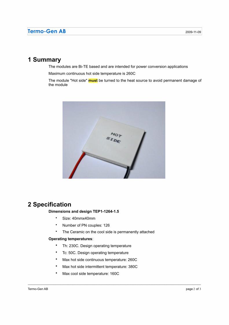
1 SummaryThe modules are Bi-TE based and are intended for power conversion applications
Maximum continuous hot side temperature is 260C
The module "Hot side" must be turned to the heat source to avoid permanent damage of the module
2 SpecificationDimensions and design TEP1-1264-1.5
• Size: 40mmx40mm• Number of PN couples: 126• The Ceramic on the cool side is permanently attached
Operating temperatures:• Th: 230C. Design operating temperature• Tc: 50C. Design operating temperature• Max hot side continuous temperature: 260C• Max hot side intermittent temperature: 380C• Max cool side temperature: 160C
Termo-Gen AB 2009-11-09
_____________________________________________________________________________________________________
Termo-Gen AB page 2 of 3

Performance at design temperature:
Open circuit voltage: 8.6VInternal resistance: 3 OhmMatch load voltage: 4.2VMatch load output current: 1.4 AMatch load output power: 5.9 WHeat flux: approximately 140 W Heat flux density: approximately 8.8 W/cm2
3 ApplicationIt is critical that the module is assembled with the "hot side" turned to the heat source to avoid permanent damage of the modules.
The ceramic wafer on the hot side is attached by a silicone for a convenient assembly of the module in the application
It is important to make sure that there always is a positive pressure (1-2 Mpa) on the module from the heat sinks. Use belleville or other spring system to allow for thermal expansion of the heat sink system and the module.
Avoid thermal shortages between the hot plate and the heat sink. Insulate mounting screws and springs
The mating surfaces must be machined flat and smooth. This is critical for efficient thermal flow and high efficiency.
The heat sink plates must be stiff to avoid warping and bending that will reduce the thermal flow and may cause damage to the modules due to high point pressures.
Apply a thin layer of thermal grease at the interfaces. Please verify the maximum temperature for the grease. We are using copper paste alternatively boron nitride powder in some high temperature applications
Termo-Gen AB Phone: +46 498 243723, Lennart Holmgren Mob: +46 708 207 534Hangvar Olarve 609 email: [email protected] 54 Lärbro http://www.termo-gen.comSweden VAT: SE556347361901
Termo-Gen AB 2009-11-09
_____________________________________________________________________________________________________
Termo-Gen AB page 3 of 3

80 Data for the thermoelectric module TEP-1265-1.5
A.3 Semiconductor properties
The semiconductor properties are given on the following two pages.

Semiconductor properties 81
r High Performance and Highly Reliable Ingot for Cooling and Power Generation Modules
Bi2Te3-Based Thermoelectric Ingot From Thermonamic
Specification of Bi2Te3-Based Thermoelectric Ingot
Description
The Bi2Te3-based thermoelectric ingot is grown by Thermonamic with the alloy of Bi, Sb, Te, Se, special doping and our unique
crystallizing processes. The Bi2Te3-based thermoelectric ingot is used to produce thermoelectric modules for cooling and heating
applications, and converting heat into electricity. Generally, the figure of merit ZT of our p-type and n-type ingots is larger than 1 at
300K, and the good feature attracts many high-end customers. Meanwhile, our ingot is featured with good mechanical strength
and highly stable property, providing the key stone for producing the high performance and reliable Peltier cooling and power
generation modules.
Features Application
High performance and reliable Peltier
cooling and power generation modules Silver-white Color
p-Type and n-type ingot ZT≥0.9@300K
Peformance Specification Sheet Options
Performance Specification p-Type n-Type Note
Diameter (mm) 31±2 31±2
Length (mm) 250± 30 250± 30
Density (gcm-3) 6.8 7.8
Suffix
Electrical
Conduction
σ(102Sm-1)
Seebeck
Coefficient
α (μVK-1)
Power Factor
P(WmK-2)
p
0: ≤1000
Geometric Characteristics (in millimeters)
Electrical Conductivity σ(102Sm-1)
850~1200 850~1200 300K
Seebeck Coefficient α (μVK-1) 190~230 180~230 300K
Thermal Conductivity κ(Wm-1K-1)
1.2~1.8 1.2~1.8 300K
Power Factor P(WmK-2) ≥0.003 ≥0.003 300K
ZT value ≥0.9 ≥0.9 300K
1:1000~1100
2: ≥1100
0: ≤190
1:190~210
2: ≥210
0: ≤0.0035
1:0.0035~0.0045
2:≥0.0045
n
0: ≤1000
1:1000~1100
2: ≥1100
0: ≤190
1:190~210
2: ≥210
0: ≤0.0035
1:0.0035~0.0045
2:≥0.0045
For Examples:P011: σ≤1000 α:190~210 P:0.0035~0.0045
N112: σ:1000~1100 α:190~210 P:≥0.0045
255±
30
φ 31± 2
p-type Ingot n-type Ingot
Tel: +86-0791-5714012 Fax: +86-791-8198660 Email: [email protected] Web Site: www.thermonamic.com/ Creative technology with fine manufacturing processes provides you the reliable and quality products.

82 Data for the thermoelectric module TEP-1265-1.5
High Performance and Highly Reliable Ingot
for Cooling and Power Generation Modules for Cooling and Power Generation Modules
Specification of Bi2Te3-Based Thermoelectric Ingot
Electrical conductivity of the Bi2Te3-based ingot Seeback coefficients of the Bi2Te3-based ingot
Operation Cautions
Caution on handling
Thermal conductivity of the Bi2Te3-based ingot Power factors of the Bi2Te3-based ingot
Z values of the Bi2Te3-based ingot ZT values of the Bi2Te3-based ingot
Storage in dry environment
Bi2Te3-Based Thermoelectric Ingot From Thermonamic
Remarks:Electrical conductivity σ and Seebeck coefficient α are measured by using a ZEM-1apparatus (Japan Vacuum Tech) in the
temperature range from 300 to 500 K. The thermal conductivity κ is obtained from the measured thermal diffusivity D, specific heat Cpand density d according to the relationship κ = D×Cp×d. Thermal diffusivity and specific heat are determined using a laser flash method(NETZSCH:LFA 457) and a power-compensation differential scanning calorimeter (TA:DSCQ20), respectively. All measurements are performed in the temperature range from 300 to 500 K.
Tel: +86-592-5714012 Fax:+86-791-8198660 Email: [email protected] Web Site: www.thermonamic.com/ Creative technology with fine manufacturing processes provides you the reliable and quality products

83
Appendix B
Module performance
B.1 Experimental setup
Figure B.1 is a picture showing a part of the experimental set up described in chapter 3.The picture is showing the electrical plate, the aluminium heat source, the thermoelectricmodule, the heat sink, and the aluminium top plate.
Figure B.1: A picture of a part of the experimental set up described in chapter 3, including the electricalplate, aluminum heat source, thermoelectric module, aluminium heat sink and aluminium top plate

84 Module performance
B.2 Raw data
The results given in section 3.3 are based on three experiments performed under threedifferent temperature differences across the module. The temperatures TH, TC, Tw,i, Tw,o
as measured for the three experiments are given in the following. Figure B.2, figure B.3and figure B.3 gives the temperatures TH and TC as a function of time for the experimentswhen ∆T = 220C , ∆T = 165C and ∆T = 105C, respectively. function of time.
Figure B.2: Measured temperatures TH, TC,Tw,i and Tw,o for experiment of ∆T = 220C. TH is measuredat two locations in the heat source aluminium plate and is represented by the red graphs. TC is measuredat two locations in the heat sink aluminum plate and is represented by the blue graphs.
The temperature TH is approximately constant and about 260 C throughout the ex-periment. We observe that the two red lines practiaclly is on top of each other. Thetemperature TC is approximately constant and about 40 C. The two blue lines rep-resenting the temperature TC measured at two locations in the heat sink aluminumplate is nearly on top of each other. We assume that the temperature distribution inthe heat source aluminium plate and heat sink aluminium plate is uniform, but frommeasurements we see that this is not totally true.
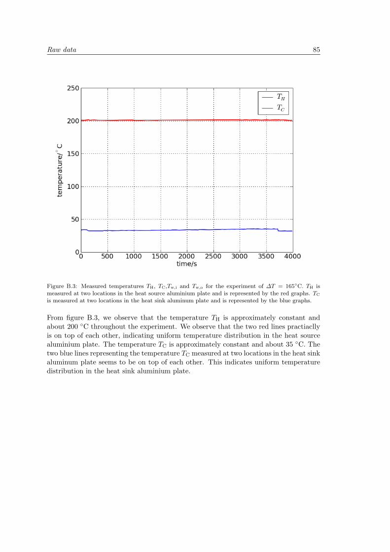
Raw data 85
Figure B.3: Measured temperatures TH, TC,Tw,i and Tw,o for the experiment of ∆T = 165C. TH ismeasured at two locations in the heat source aluminium plate and is represented by the red graphs. TC
is measured at two locations in the heat sink aluminum plate and is represented by the blue graphs.
From figure B.3, we observe that the temperature TH is approximately constant andabout 200 C throughout the experiment. We observe that the two red lines practiacllyis on top of each other, indicating uniform temperature distribution in the heat sourcealuminium plate. The temperature TC is approximately constant and about 35 C. Thetwo blue lines representing the temperature TC measured at two locations in the heat sinkaluminum plate seems to be on top of each other. This indicates uniform temperaturedistribution in the heat sink aluminium plate.

86 Module performance
Figure B.4: Measured temperatures TH, TC,Tw,i and Tw,o for the experiment of ∆T = 105C. TH ismeasured at two locations in the heat source aluminium plate and is represented by the red graphs. TC
is measured at two locations in the heat sink aluminum plate and is represented by the blue graphs.
The temperature TH is approximately constant and about 130 C throughout the exper-iment. We observe that the two red lines practiaclly is on top of each other, indicatinguniform temperature distribution in the heat source aluminium plate. We observe thatTC varies slightly throughouth the experiments, this may be due to the fact that heattransfer through the device changes as the current through the device changes. TC isassumed to be constant, even though it varies. The two blue lines representing the tem-perature TC measured at two locations in the heat sink aluminum plate seems to beon top of each other. This indicates uniform temperature distribution in the heat sinkaluminium plate.
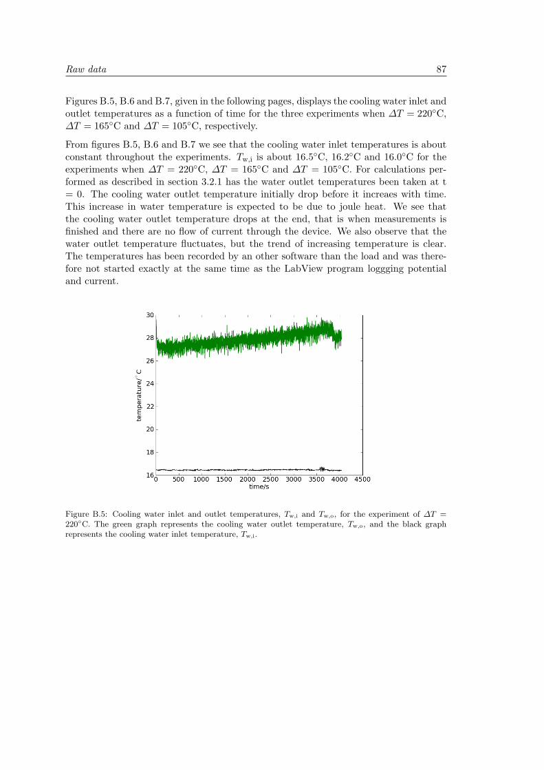
Raw data 87
Figures B.5, B.6 and B.7, given in the following pages, displays the cooling water inlet andoutlet temperatures as a function of time for the three experiments when ∆T = 220C,∆T = 165C and ∆T = 105C, respectively.
From figures B.5, B.6 and B.7 we see that the cooling water inlet temperatures is aboutconstant throughout the experiments. Tw,i is about 16.5C, 16.2C and 16.0C for theexperiments when ∆T = 220C, ∆T = 165C and ∆T = 105C. For calculations per-formed as described in section 3.2.1 has the water outlet temperatures been taken at t= 0. The cooling water outlet temperature initially drop before it increaes with time.This increase in water temperature is expected to be due to joule heat. We see thatthe cooling water outlet temperature drops at the end, that is when measurements isfinished and there are no flow of current through the device. We also observe that thewater outlet temperature fluctuates, but the trend of increasing temperature is clear.The temperatures has been recorded by an other software than the load and was there-fore not started exactly at the same time as the LabView program loggging potentialand current.
Figure B.5: Cooling water inlet and outlet temperatures, Tw,i and Tw,o, for the experiment of ∆T =220C. The green graph represents the cooling water outlet temperature, Tw,o, and the black graphrepresents the cooling water inlet temperature, Tw,i.

88 Module performance
Figure B.6: Cooling water inlet and outlet temperatures, Tw,i and Tw,o, for the experiment of ∆T =165C. The green graph represents the cooling water outlet temperature, Tw,o, and the black graphrepresents the cooling water inlet temperature, Tw,i.
Figure B.7: Cooling water inlet and outlet temperatures, Tw,i and Tw,o, for the experiment of ∆T =105C. The green graph represents the cooling water outlet temperature, Tw,o, and the black graphrepresents the cooling water inlet temperature, Tw,i.

Cooling water volume flow 89
B.3 Cooling water volume flow
The cooling water volume flows for the three experiments are given in table B.1. Thevolume flow was measured as described in section 3.2, in five parallels. The volume flowfor the experiments when ∆T = 165C and ∆T = 105C was taken as the same as theexperiments was performed consecutively.
Table B.1: Time to fill a 100 mL measuring glass, calculated volume flow and average volume flow.
Experiment time (s) Volume flow (mL/s) average volume flow∆T = 220c 34.1 2.93
33.9 2.9433.9 2.9433.9 2.9434.1 2.93
2.94 ±0.1∆T = 165C and ∆T = 105C 33.9 2.94
34.3 2.9234.0 2.9434.1 2.9333.9 2.95
2.93 ±0.2


91
Appendix C
Calorimetric study
C.1 Experimental set up
Pictures of the calorimeter, figure 4.1, used for the calorimetric study of the thermoelec-tric module TEP-1264-1.5 are given in the following.
Figure C.1 displays a picture showing half of the calorimeter described in section 4.1.1and figure 4.1. The picture displays the left hand side of the calorimeter pluss thethermoelectric module and the aluminium plate belonging to the right hand side in thecalorimeter.
Figure C.1: Picture of half of the calorimeter described in section 4.1.1 and figure 4.1. The picturedisplays the left hand side of the calorimeter pluss the thermoelectric module and the aluminium platebelonging to the right hand side in the calorimeter.

92 Calorimetric study
Figure C.2 displays a picture of the calorimeter described in section 4.1.1 and figure 4.1.The picture is taken at the location where the experiments are performed. Figure C.3displays a picture of the calorimeter, described in section 4.1.1 and figure 4.1, with thelayer of isolating expanded polyester.
Figure C.2: A picture displaying the calorimeter described in section 4.1.1 and figure 4.1. Picture istaken at the location where experiments were conducted.
Figure C.3: A picture displaying the calorimeter described in section 4.1.1 and figure 4.1, with the layerof isolating expanded polyester. Picture is taken at the location where experiments were conducted.

Raw data for calorimetric studies 93
C.2 Raw data for calorimetric studies
C.2.1 Experiment type II
The results given in section 4.2.2 and section 4.2.4 are based on data obtained from threeexperiments of type II. We present the measured parameters as a function of time forexperiment 1 of type II. The purpose is to show how the measured parameters respond toa change in applied voltage, U, and to see how the measured parameters fluctuates andstabilize as a function of time. Then we present data for the three type II experiments,used for calculating the results given in sections 4.2.2 and 4.2.4.
Figure C.4 shows the effect added to the two heaters at the left and right hand side ofthe device in the calorimeter, see figure 4.1, and the voltage applied to the device as afunction of time. The left- and right- hand sides of the calorimeter are referred to as theH- and C-sides hereafter. The red curve refers to the effect added to the heater at the Hside, Qadd,H, and the green curve refers to the effect added to the heater at the C side,Qadd,C.
Figure C.4: Effect added to the two heaters in the calorimeter and voltage, U, as a function of time forexperiment 1 of type II. The green curve is the effect added to the heater at the C-side, Qadd,C, andthe red curve is the effect added to the H-side, Qadd,H, of the thermoelectric device. See figure 4.1 forexplanation of notation. The black curve is the voltage applied to the thermoelectric device as a functionof time.
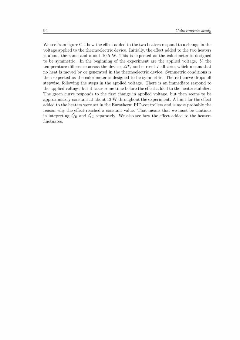
94 Calorimetric study
We see from figure C.4 how the effect added to the two heaters respond to a change in thevoltage applied to the thermoelectric device. Initially, the effect added to the two heatersis about the same and about 10.5 W. This is expected as the calorimeter is designedto be symmetric. In the beginning of the experiment are the applied voltage, U, thetemperature difference across the device, ∆T , and current I all zero, which means thatno heat is moved by or generated in the thermoelectric device. Symmetric conditions isthen expected as the calorimeter is designed to be symmetric. The red curve drops offstepwise, following the steps in the applied voltage. There is an immediate respond tothe applied voltage, but it takes some time before the effect added to the heater stabilize.The green curve responds to the first change in applied voltage, but then seems to beapproximately constant at about 13 W throughout the experiment. A limit for the effectadded to the heaters were set in the Eurotherm PID-controllers and is most probably thereason why the effect reached a constant value. That means that we must be cautiousin intepreting QH and QC separately. We also see how the effect added to the heatersfluctuates.

Raw data for calorimetric studies 95
Figure C.5 shows the temperatures of the aluminium plates next to the thermoelectricdevice, see figure 4.1, as a function of time for experiment 1 of type II. Red curve refersto TH,1 and green curve refers to TC,1. The black curve is the voltage, U, applied to thethermoelectric device, plotted as a function of time.
Figure C.5: Temperatures TH,1 and TC,1, see figure 4.1, and the applied voltage, U, as a function oftime for experiment 1 of type II. Red curve refers to the temperature TH,1, green curve refers to thetemperature TC,1 and black curve refers to the voltage applied, U.
We see from figure C.5 that there is an immediate respons in the temperatures TH,1 andTC,1 when the voltage applied is changed. Temperature TH,1 makes a jump and thenstabilise again. The temperature TH,1 is approximately constant about 51C throughoutthe experiment. TC,1 drops off as the voltage is increased. The calorimeter is designed tobe isothermal, and a drop of temperature is therefore not expected. The current throughthe device will increase as the voltage increases, and the device will move more heat fromthe C-side to the H- side. As there was a limit on the effect added to the heaters willnot enough effect be added to the heaters at the C-side in order to compensate for theheat moved from the C-side to the H-side. As a consequence of this will the temperatureTC,1 drop off as the voltage is increased.

96 Calorimetric study
Figure C.6 shows the current, I, through the device and the voltage, U, applied to thedevice as a function of time for experiment 1 of type II.Wee see from figure C.6 howthe current responds to the voltage applied, the current make a jump immediately whenvoltage is increased and then stabilize.
Figure C.6: Current, I, through the thermoelectric module and voltage, U, applied to the module asa function of time for experiment 1 of type II. The blue curve is the current and the black line is thevoltage.
Figure C.7 shows the temperatures TH,1, TC,1, TH,0 and TC,0 for all three type II ex-periments as a function of voltage, U, applied to the device. The temperatures shownin this figure are average temperatures. Averages were taken when measurements hadstabilized after a change to the applied voltage, U, was done. We see that the temper-ature TH,0 is approximately constant and about 51C as the voltage is increased. TC,0
decreases as the voltage increases. The calorimeter is designed to be isothermal, and areason for this temperature drop may be the limit on the effect added to the heaters.The temperature of the two end plates are approximately constant and about 10C asthe voltage is increased.

Raw data for calorimetric studies 97
Figure C.7: Measured temperatures for all three type II experiments plotted versus voltage applied to thethermoelectric device, U. Temperatures are average temperatures. Triangles represents the temperatureTH,1, cross represents the temperature TC,1, dots represents the temperature TH,0 and squares representsthe temperature TC,0. See figure 4.1 for explanation.
Figure C.8 shows the average effects added to the heaters for all three type II experimentsas a function of the voltage applied, U. Averages were taken when measurements hadstabilized. Square represents the heat added to the heater at the H-side, Qadd,H, anddots represents the heat added to the heater at the C-side, Qadd,C. We see that the heatadded to the two sides in the calorimeter is asymmetric. The effect added to the heaterat the H-side, Qadd,H, drop off as the voltage increases. The effect added to the C-side,Qadd,C, increases from an initial value of about 10.5 W to about 13W as the voltage isincreased from 0 V to 0.5 V. As the voltage is increased further is Qadd,C approximatelyconstant and about 13 W. Symmetri was expected as the calorimeter is designed to besymmetric, but asymmetric behaviour The limit on the effect added to the heaters maybe the reason for this asymmetric behaviour. Asymmetry in the heat added to the twoheaters coincides to the observed drop in the temperature TC,0.
Figure C.9 displays a plot of current, I, versus applied voltage U. The current is givenas the average current when measurements had stabilized.
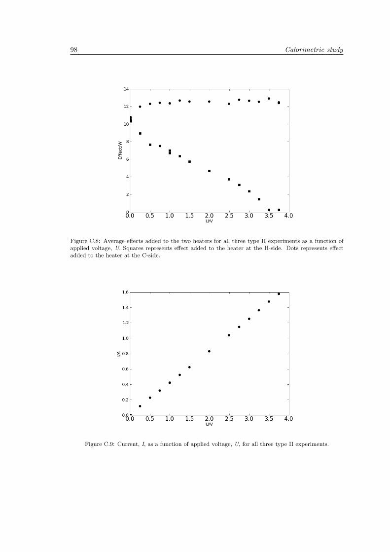
98 Calorimetric study
Figure C.8: Average effects added to the two heaters for all three type II experiments as a function ofapplied voltage, U. Squares represents effect added to the heater at the H-side. Dots represents effectadded to the heater at the C-side.
Figure C.9: Current, I, as a function of applied voltage, U, for all three type II experiments.

Raw data for calorimetric studies 99
C.2.2 Experiment type III
The results presented in section 4.2.3 are based on data from one type III experiment.The raw data which provides the basis for the results given in section 4.2.3 are presentedin the following.
The effect added to the two heaters for the experiment type III is plotted as a functionof time and shown in figure C.10. The red curve represents the effect added to the heaterat the H-side, Qadd,H, and the green curve represents the effect added to the heater atthe C-side, Qadd,C, in the calorimeter. See figure 4.1 for explanation of notation.
Figure C.10: Effect added to the two heaters in the calorimeter as a function of time for the experimentof type III. The green curve is the effect added to the heater at the C-side,Qadd,C, and the red curveis the effect added to the H-side,Qadd,H, of the thermoelectric device. See figure 4.1 for explanation ofnotation.
The effects added to the heaters at each side is both about 10 W at the start of theexperiment. That is when no current is flowing through the device and when there is notemperature difference acorss the device, I = 0 and ∆T = 0.
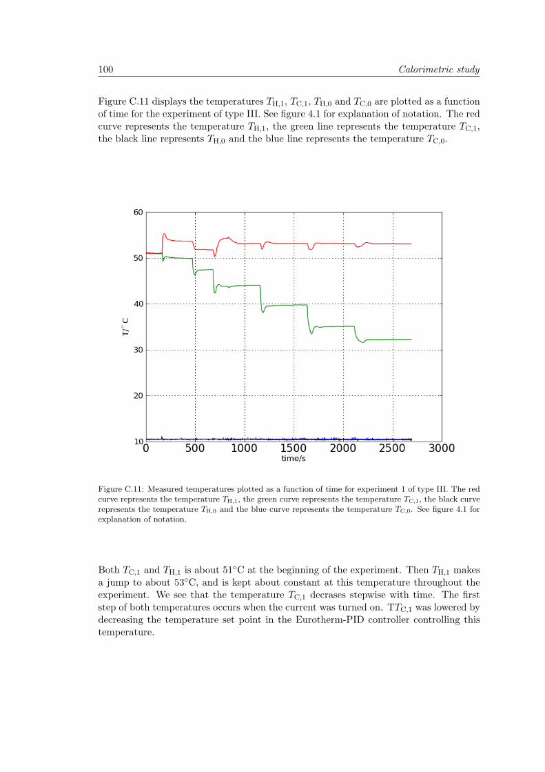
100 Calorimetric study
Figure C.11 displays the temperatures TH,1, TC,1, TH,0 and TC,0 are plotted as a functionof time for the experiment of type III. See figure 4.1 for explanation of notation. The redcurve represents the temperature TH,1, the green line represents the temperature TC,1,the black line represents TH,0 and the blue line represents the temperature TC,0.
Figure C.11: Measured temperatures plotted as a function of time for experiment 1 of type III. The redcurve represents the temperature TH,1, the green curve represents the temperature TC,1, the black curverepresents the temperature TH,0 and the blue curve represents the temperature TC,0. See figure 4.1 forexplanation of notation.
Both TC,1 and TH,1 is about 51C at the beginning of the experiment. Then TH,1 makesa jump to about 53C, and is kept about constant at this temperature throughout theexperiment. We see that the temperature TC,1 decrases stepwise with time. The firststep of both temperatures occurs when the current was turned on. TTC,1 was lowered bydecreasing the temperature set point in the Eurotherm-PID controller controlling thistemperature.

Raw data for calorimetric studies 101
Figure C.12 displays the current I through the device as a function of time for the typeIII experiment.
Figure C.12: The current I through the device as a function of time for the type III experiment.