recovering communities in the general stochastic block model without ... · recovering communities...

Recovering communities in the general stochastic block model

without knowing the parameters

Emmanuel Abbe∗ Colin Sandon†

June 12, 2015

Abstract

Most recent developments on the stochastic block model (SBM) rely on the knowledgeof the model parameters, or at least on the number of communities. This paper introducesefficient algorithms that do not require such knowledge and yet achieve the optimalinformation-theoretic tradeoffs identified in [AS15] for linear size communities. Theresults are three-fold: (i) in the constant degree regime, an algorithm is developedthat requires only a lower-bound on the relative sizes of the communities and detectscommunities with an optimal accuracy scaling for large degrees; (ii) in the regimewhere degrees are scaled by ω(1) (diverging degrees), this is enhanced into a fullyagnostic algorithm that only takes the graph in question and simultaneously learns themodel parameters (including the number of communities) and detects communities withaccuracy 1− o(1), with an overall quasi-linear complexity; (iii) in the logarithmic degreeregime, an agnostic algorithm is developed that learns the parameters and achievesthe optimal CH-limit for exact recovery, in quasi-linear time. These provide the firstalgorithms affording efficiency, universality and information-theoretic optimality forstrong and weak consistency in the general SBM with linear size communities.

∗Program in Applied and Computational Mathematics, and EE department, Princeton University, Prince-ton, USA, [email protected]. This research was partially supported by the 2014 Bell Labs Prize.

†Department of Mathematics, Princeton University, USA, [email protected].

arX

iv:1

506.

0372

9v1

[m

ath.

PR]

11

Jun

2015

Contents

1 Introduction 11.1 Related results on the general SBM with known parameters . . . . . . . . . 21.2 Estimating the parameters . . . . . . . . . . . . . . . . . . . . . . . . . . . . 4

2 Results 42.1 Definitions and terminologies . . . . . . . . . . . . . . . . . . . . . . . . . . 42.2 Partial recovery . . . . . . . . . . . . . . . . . . . . . . . . . . . . . . . . . . 52.3 Exact recovery . . . . . . . . . . . . . . . . . . . . . . . . . . . . . . . . . . 6

3 Proof Techniques and Algorithms 63.1 Partial recovery and the Agnostic-sphere-comparison algorithm . . . . . 63.2 Exact recovery and the Agnostic-degree-profiling algorithm . . . . . . 10

4 An example with real data 11

5 Open problems 12

6 The Agnostic-sphere-comparison algorithm in details 16

7 Appendix 247.1 Partial Recovery . . . . . . . . . . . . . . . . . . . . . . . . . . . . . . . . . 24

7.1.1 Formal results . . . . . . . . . . . . . . . . . . . . . . . . . . . . . . 247.1.2 Proof of Theorem 6 . . . . . . . . . . . . . . . . . . . . . . . . . . . 25

7.2 Exact recovery . . . . . . . . . . . . . . . . . . . . . . . . . . . . . . . . . . 497.2.1 Formal results . . . . . . . . . . . . . . . . . . . . . . . . . . . . . . 497.2.2 Testing degree profiles . . . . . . . . . . . . . . . . . . . . . . . . . . . 517.2.3 Proof of Theorem 7 . . . . . . . . . . . . . . . . . . . . . . . . . . . 57

1 Introduction

This paper studies the problem of recovering communities in the general stochastic blockmodel with linear size communities, for constant and slowly diverging degree regimes. Incontrast to [AS15], this paper does not require knowledge of the SBM parameters. Inparticular, the problem of learning the model parameters is solved when average degrees arediverging. We next provide some motivations on the problem and further background onthe model.

Detecting communities (or clusters) in graphs is a fundamental problem in networks,computer science and machine learning. This applies to a large variety of complex networks(e.g., social and biological networks) as well as to data sets engineered as networks viasimilarly graphs, where one often attempts to get a first impression on the data by tryingto identify groups with similar behavior. In particular, finding communities allows oneto find like-minded people in social networks [GN02, NWS], to improve recommendationsystems [LSY03, XWZ+14], to segment or classify images [SM97, SHB07], to detect proteincomplexes [CY06, MPN+99], to find genetically related sub-populations [PSD00, JTZ04],or discover new tumor subclasses [SPT+01].

While a large variety of community detection algorithms have been deployed in thepast decades, the understanding of the fundamental limits of community detection hasonly appeared more recently, in particular for the SBM [Co10, DKMZ11, Mas14, MNS14,ABH14, MNSb, YC14, AS15]. The SBM is a canonical model for community detection[HLL83, WBB76, FMW85, WW87, BC09, KN11, BCLS87, DF89, Bop87, JS98, CK99,CI01, SN97, McS01, BC09, RCY11, CWA12, CSX12], where n vertices are partitioned intok communities of relative size pi, i ∈ [k], and pairs of nodes in communities i and j connectindependently with probability Wi,j .

Recently the SBM came back to the center of the attention at both the practical level,due to extensions allowing overlapping communities [ABFX08] that have proved to fit wellreal data sets in massive networks [GB13], and at the theoretical level due to new phasetransition phenomena [Co10, DKMZ11, Mas14, MNS14, ABH14, MNSb]. The latter worksfocus exclusively on the SBM with two symmetric communities, i.e., each community is of thesame size and the connectivity in each community is identical. Denoting by p the intra- and qthe extra-cluster probabilities, most of the results are concerned with two figure of merits: (i)recovery (also called exact recovery or strong consistency), which investigates the regimesof p and q for which there exists an algorithm that recovers with high probability the twocommunities completely [BCLS87, DF89, Bop87, JS98, CK99, CI01, SN97, McS01, BC09,RCY11, CWA12, CSX12, Vu14, YC14], (ii) detection, which investigates the regimes forwhich there exists an algorithm that recovers with high probability a positively correlatedpartition [Co10, DKMZ11, MNS12, Mas14, MNS14].

The sharp threshold for exact recovery was obtained in [ABH14, MNSb], showing1

that for p = a log(n)/n, q = b log(n)/n, a, b > 0, exact recovery is solvable if and only if√a−√b ≥ 2, with efficient algorithms achieving the threshold provided in [ABH14, MNSb].

In addition, [ABH14] introduces an SDP proved to achieve the threshold in [BH14, Ban15],while [YP14] shows that a spectral algorithm also achieves the threshold. Prior to these,

1[MNSb] generalizes this to a, b = Θ(1).

1

the sharp threshold for detection was obtained in [Mas14, MNS14], showing that detectionis solvable (and so efficiently) if and only if (a − b)2 > 2(a + b), when p = a/n, q = b/n,settling a conjecture made in [DKMZ11] and improving on [Co10].

Besides the detection and the recovery properties, one may ask about the partial recoveryof the communities, studied in [MNSa, GV14, Vu14, CRV15, AS15]. Of particular interest tothis paper is the case of almost exact recovery (also called weak consistency), where only avanishing fraction of the nodes is allowed to be misclassified. For two-symmetric communities,[MNSb] shows that almost exact recovery is possible if and only if n(p− q)2/(p+ q) diverges,generalized in [AS15] for general SBMs.

In the next section, we discuss the results for the general SBM of interest in this paperand the problem of learning the model parameters. We conclude this section by providingmotivations on the problem of achieving the threshold with an efficient and universalalgorithm.

Threshold phenomena have long been studied in fields such as information theory (e.g.,Shannon’s capacity) and constraint satisfaction problems (e.g., the SAT threshold). Inparticular, the quest of achieving the threshold has generated major algorithmic developmentsin these fields (e.g., LDPC codes, polar codes, survey propagation to name a few). Likewise,identifying thresholds in community detection models is key to benchmark and guide thedevelopment of clustering algorithms. Most reasonable algorithms may succeed in someregimes, while in others they may be doomed to fail due to computational barriers. However,it is particularly crucial to develop benchmarks that do not depend sensitively on theknowledge of the model parameters. A natural question is hence whether one can solvethe various recovery problems in the SBM without having access to the parameters. Thispaper answers this question by the affirmative for the exact and almost exact recovery ofthe communities.

1.1 Related results on the general SBM with known parameters

Most of the previous works are concerned with the SBM having symmetric communities(mainly 2 or sometimes k), with the exception of [Vu14] which provides some achievabilityresults for the general SBM.2 Recently, [AS15] studied the fundamental limits for the generalSBM, with results as follows (where SBM(n, p,W ) is the SBM with community prior p andconnectivity matrix W ).

I. Partial and almost exact recovery in the general SBM. The first result of [AS15]concerns the regime where the connectivity matrix scales as Q/n for a positive symmetricmatrix Q (i.e., the node average degree is constant). The following notion of SNR isintroduced3

SNR = |λmin|2/λmax (1)

2[GV14] also study variations of the k-symmetric model.

3Note that this in a sense the “worst-case” notion of SNR, which ensures that all of the communitiescan be separated (when amplified); one could consider other ratios of the kind |λj |2/λmax, for subsequenteigenvalues (j = 2, 3, . . . ), if interested in separating only subset of the communities.

2

where λmin and λmax are respectively the smallest4 and largest eigenvalue of diag(p)Q.The algorithm Sphere-comparison is proposed that solves partial recovery with expo-

nential accuracy and quasi-linear complexity when the SNR diverges, solving in particularalmost exact recovery.

Theorem 1. [AS15] Given any k ∈ Z, p ∈ (0, 1)k with |p| = 1, and symmetric matrix Qwith no two rows equal, let λ be the largest eigenvalue of PQ, and λ′ be the eigenvalue of

PQ with the smallest nonzero magnitude. If ρ := |λ′|2λ > 4, λ7 < (λ′)8, and 4λ3 < (λ′)4,

then for some ε = ε(λ, λ′) and C = C(p,Q) > 0, Sphere-comparison (see Section 3.1)detects with high probability communities in graphs drawn from SBM(n, p,Q/n) with accuracy

1−4ke−Cρ16k /(1−exp(− Cρ

16k

((λ′)4

λ3− 1)

)), provided that the above is larger than 1− mini pi2 ln(4k) , and

runs in O(n1+ε) time. Moreover, ε can be made arbitrarily small with 8 ln(λ√

2/|λ′|)/ ln(λ),and C(p, αQ) is independent of α.

Note that for k symmetric clusters, SNR reduces to (a−b)2k(a+(k−1)b) , which is the quantity of

interest for detection [DKMZ11, MNS12]. Moreover, the SNR must diverge to ensure almostexact recovery in the symmetric case [AS15]. The following is an important consequence ofthe previous theorem, as it shows that Sphere-comparison achieves almost exact recoverywhen the entries of Q are scaled.

Corollary 1. [AS15] For any k ∈ Z, p ∈ (0, 1)k with |p| = 1, and symmetric matrix Q withno two rows equal, there exists ε(δ) = O(1/ ln(δ)) such that for all sufficiently large δ thereexists an algorithm (Sphere-comparison) that detects communities in graphs drawn fromSBM(n, p, δQ) with accuracy 1− e−Ω(δ) and complexity On(n1+ε(δ)).

II. Exact recovery in the general SBM. The second result in [AS15] is for the regimewhere the connectivity matrix scales as log(n)Q/n, Q fixed, where it is shown that exactrecovery has a sharp threshold characterized by the divergence function

D+(f, g) = maxt∈[0,1]

∑x∈[k]

(tf(x) + (1− t)g(x)− f(x)tg(x)1−t) ,

named the CH-divergence in [AS15]. Specifically, if all pairs of columns in diag(p)Q are atD+-distance at least 1 from each other, then exact recovery is solvable in the general SBM.This provides in particular an operational meaning to a new divergence function analog tothe KL-divergence in the channel coding theorem (see Section 2.3 in [AS15]). Moreover, analgorithm (Degree-profiling) is developed that solves exact recovery down to the D+ limitin quasi-linear time, showing that exact recovery has no informational to computational gap(as opposed to the conjectures made for detection with more than 4 communities [DKMZ11]).The following gives a more general statement characterizing which subset of communitiescan be extracted — see Definition 3 for formal definitions.

Theorem 2. [AS15] (i) Exact recovery is solvable in the stochastic block model G2(n, p,Q)for a partition [k] = tts=1As if and only if for all i and j in different subsets of the partition,5

D+((PQ)i, (PQ)j) ≥ 1, (2)

4The smallest eigenvalue of diag(p)Q is the one with least magnitude.

5The entries of Q are assumed to be non-zero.

3

In particular, exact recovery is information-theoretically solvable in SBM(n, p,Q log(n)/n) ifand only if mini,j∈[k],i 6=j D+((PQ)i||(PQ)j) ≥ 1.(ii) The Degree-profiling algorithm (see [AS15]) recovers the finest partition that can berecovered with probability 1 − on(1) and runs in o(n1+ε) time for all ε > 0. In particular,exact recovery is efficiently solvable whenever it is information-theoretically solvable.

In summary, exact or almost exact recovery is closed for the general SBM (and detectionis closed for 2 symmetric communities). However this is for the case where the parametersof the SBM are assumed to be known, and with linear-size communities.

1.2 Estimating the parameters

For the estimation of the parameter, some results are known for two-symmetric communities.In the logarithmic degree regime, since the SDP is agnostic to the parameters (it is arelaxation of the min-bisection), and the parameters can be estimated by recovering thecommunities [ABH14, BH14, Ban15]. For the constant-degree regime, [MNS12] shows thatthe parameters can be estimated above the threshold by counting cycles (which is efficientlyapproximated by counting non-backtracking walks). These are however for a fixed numberof communities, namely 2. We also became recently aware of a parallel work [BCS15], whichconsiders private graphon estimation (including SBMs). In particular, for the logarithmicdegree regime, [BCS15] obtains a procedure to estimate parameters of graphons in anappropriate version of the L2 norm. This procedure is however not efficient.

For the general SBM, the results of [AS15] allow to find communities efficiently, howeverthese rely on the knowledge of the parameters. Hence, a major open problem is to understandif these results can be extended without such a knowledge.

2 Results

Agnostic algorithms are developed for the constant and diverging node degrees. Theseafford optimal accuracy scaling for large node degrees and achieve the CH-divergence limitfor logarithmic node degrees in quasi-linear time. In particular, these solve the parameterestimation problems for SBM(n, p, ω(1)Q) without knowing the number of communities. Anexample with real data is provided in Section 4.

2.1 Definitions and terminologies

The general stochastic block model SBM(n, p,W ) is a random graph ensemble defined onthe vertex-set V = [n], where each vertex v ∈ V is assigned independently a hidden (orplanted) label σv in [k] under a probability distribution p = (p1, . . . , pk) on [k], and each(unordered) pair of nodes (u, v) ∈ V ×V is connected independently with probability Wσu,σv ,where Wσu,σv is specified by a symmetric k × k matrix W with entries in [0, 1]. Note thatG ∼ SBM(n, p,W ) denotes a random graph drawn under this model, without the hidden(or planted) clusters (i.e., the labels σv ) revealed. The goal is to recover these labels byobserving only the graph.

This paper focuses on p independent of n (the communities have linear size), W dependenton n such that the average node degrees are either constant or logarithmically growing, and

4

k fixed. These assumptions on p and k could be relaxed, for example to slowly growing k,but we leave this for future work. As discussed in the introduction, the above regimes forW are both motivated by applications, as networks are typically sparse [LLDM08, Str01]though the average degrees may not be small, and by the fact that interesting mathematicalphenomena take place in these regimes. For convenience, we attribute specific notations forthe model in these regimes:

Definition 1. For a symmetric matrix Q ∈ Rk×k+ , G1(n, p,Q) denotes SBM(n, p,Q/n), andG2(n, p,Q) denotes SBM(n, p, ln(n)Q/n).

Definition 2. (Partial recovery.) An algorithm recovers or detects communities in SBM(n, p,W )with an accuracy of α ∈ [0, 1], if it outputs a labelling of the nodes σ′(v), v ∈ V , whichagrees with the true labelling σ on a fraction α of the nodes with probability 1− on(1). Theagreement is maximized over relabellings of the communities.

Definition 3. (Exact recovery.) Exact recovery is solvable in SBM(n, p,W ) for a communitypartition [k] = tts=1As, where As is a subset of [k], if there exists an algorithm that takesG ∼ SBM(n, p,W ) and assigns to each node in G an element of A1, . . . , At that containsits true community6 with probability 1− on(1). Exact recovery is solvable in SBM(n, p,W ) ifit is solvable for the partition of [k] into k singletons, i.e., all communities can be recovered.

The problem is solvable information-theoretically if there exists an algorithm that solvesit, and efficiently if the algorithm runs in polynomial-time in n. Note that exact recoveryfor the partition [k] = i t ([k] \ i) is equivalent to extracting community i. In general,recovering a partition [k] = tts=1As is equivalent to merging the communities that are in acommon subset As and recovering the merged communities. Note also that exact recoveryin SBM(n, p,W ) requires the graph not to have vertices of degree 0 in multiple communitieswith high probability (i.e., connectivity in the symmetric case). Therefore, for exact recovery,

we focus below on W = ln(n)n Q where Q is fixed.

2.2 Partial recovery

Our main result in the Appendix (Theorme 6) applies to SBM(n, p,Q/n) with arbitrary Q.We provided here a specific instance which is easier to parse.

Theorem 3 (See Theorem 6). Given δ > 0 and for any k ∈ Z, p ∈ (0, 1)k with∑pi = 1

and 0 < δ ≤ min pi, and any symmetric matrix Q with no two rows equal such that everyentry in Qk is positive (in other words, Q such that there is a nonzero probability of a pathbetween vertices in any two communities in a graph drawn from G1(n, p, cQ)), there existsε(c) = O(1/ ln(c)) such that for all sufficiently large c, Agnostic-sphere-comparison(G, δ)detects communities in graphs drawn from G1(n, p, cQ) with accuracy at least 1− e−Ω(c) inOn(n1+ε(c)) time.

Note that a vertex in community i has degree 0 with probability exponential in c, andthere is no way to differentiate between vertices of degree 0 from different communities. So,

6This is again up to relabellings of the communities.

5

an error rate that decreases exponentially with c is optimal. The above gives in particularthe parameter estimation in the case c = ω(1) (see also Lemma 17 in the Appendix).

The general result in the Appendix yields the following refined results in the k-blocksymmetric case.

Theorem 4. Consider the k-block symmetric case. In other words, pi = 1k for all i, and

Qi,j is α if i = j and β otherwise. The vector whose entries are all 1s is an eigenvector of

PQ with eigenvalue α+(k−1)βk , and every vector whose entries add up to 0 is an eigenvector

of PQ with eigenvalue α−βk . So, λ = α+(k−1)β

k and λ′ = α−βk and (λ′)2

λ = (a−b)2k(a+(k−1)β) . Then,

as long as 1609 k(α+ (k − 1)β)7 < (α− β)8 and 4k(α+ (k − 1)β)3 < (α− β)4, there exist a

constant c > 0 such that Agnostic-sphere-comparison(G, 1/k) detects communities withan accuracy of 1−O(e−c(α−β)2/(α+(k−1)β)) for sufficiently large (α− β)2/(α+ (k − 1)β).

We refer to Section 4 for an example of implementation with real data.

2.3 Exact recovery

Recall that from [AS15], exact recovery is information-theoretically solvable in the stochasticblock model G2(n, p,Q) for a partition [k] = tts=1As if and only if for all i and j in differentsubsets of the partition,

D+((PQ)i, (PQ)j) ≥ 1. (3)

We next show that this can be achieved without knowing the parameters. Recall that thefinest partition is the largest partition of [k] that ensure (19).

Theorem 5. (See Theorem 7) The Agnostic-degree-profiling algorithm (see Section3.2) recovers the finest partition in any G2(n, p,Q), it uses no input except the graph inquestion, and runs in o(n1+ε) time for all ε > 0. In particular, exact recovery is efficientlyand universally solvable whenever it is information-theoretically solvable.

The proof assumes that the entries of Q are non-zero, see Remark 1 for zero entries.To achieve this result we rely on a two step procedure. First an algorithm is developedto recover all but a vanishing fraction of nodes — this is the main focus of our partialrecovery result — and then a procedure is used to “clean up” the leftover graphs using thenode degrees of the preliminary classification. This turns out to be much more efficientthan aiming for an algorithm that directly achieves exact recovery. We already used thistechnique in [AS15], but here we also deal with the difficulties resulting from not knowingthe SBM’s parameters.

3 Proof Techniques and Algorithms

3.1 Partial recovery and the Agnostic-sphere-comparison algorithm

The first key observation used to classify graphs’ vertices is that if v is a vertex in a graphdrawn from G1(n, p,Q) then for all small r the expected number of vertices in community ithat are r edges away from v is approximately ei · (PQ)reσv . So, we define:

6

Definition 4. For any vertex v, let Nr(v) be the set of all vertices with shortest path to v oflength r. We also refer to the vector with i-th entry equal to the number of vertices in Nr(v)that are in community i as Nr(v). If there are multiple graphs that v could be considered avertex in, let Nr[G](v) be the set of all vertices with shortest paths in G to v of length r.

One could probably determine PQ and eσ given the values of (PQ)reσv for a few differentr, but using Nr(v) to approximate that would require knowing how many of the verticesin Nr(v) are in each community. So, we attempt to get information relating to how manyvertices in Nr(v) are in each community by checking how it connects to Nr′(v

′) for somevertex v′ and integer r′. The obvious way to do this would be to compute the cardinality oftheir intersection. Unfortunately, whether a given vertex in community i is in Nr(v) is notindependent of whether it is in Nr′(v

′), which causes the cardinality of |Nr(v) ∩Nr′(v′)| to

differ from what one would expect badly enough to disrupt plans to use it for approximations.In order to get around this, we randomly assign every edge in G to a set E with probability

c. We hence define the following.

Definition 5. For any vertices v, v′ ∈ G, r, r′ ∈ Z, and subset of G’s edges E, let Nr,r′[E](v ·v′) be the number of pairs of vertices (v1, v2) such that v1 ∈ Nr[G\E](v), v2 ∈ Nr′[G\E](v

′),and (v1, v2) ∈ E.

Note that E and G\E are disjoint; however, G is sparse enough that even if they weregenerated independently a given pair of vertices would have an edge between them inboth with probability O( 1

n2 ). So, E is approximately independent of G\E. Thus, for anyv1 ∈ Nr[G/E](v) and v2 ∈ Nr′[G/E](v

′), (v1, v2) ∈ E with a probability of approximatelycQσv1 ,σv2/n. As a result,

Nr,r′ [E](v · v′) ≈ Nr[G\E](v) · cQnNr′[G\E](v

′)

≈ ((1− c)PQ)reσv ·cQ

n((1− c)PQ)r

′eσv′

= c(1− c)r+r′eσv ·Q(PQ)r+r′eσv′/n

Let λ1, ..., λh be the distinct eigenvalues of PQ, ordered so that |λ1| ≥ |λ2| ≥ ... ≥ |λh| ≥0. Also define h′ so that h′ = h if λh 6= 0 and h′ = h− 1 if λh = 0. If Wi is the eigenspace ofPQ corresponding to the eigenvalue λi, and PWi is the projection operator on to Wi, then

Nr,r′[E](v · v′) ≈ c(1− c)r+r′eσv ·Q(PQ)r+r

′eσv′/n (4)

=c(1− c)r+r′

n

(∑i

PWi(eσv)

)·Q(PQ)r+r

′

∑j

PWj (eσv′ )

(5)

=c(1− c)r+r′

n

∑i,j

PWi(eσv) ·Q(PQ)r+r′PWj (eσv′ ) (6)

=c(1− c)r+r′

n

∑i,j

PWi(eσv) · P−1(λj)r+r′+1PWj (eσv′ ) (7)

=c(1− c)r+r′

n

∑i

λr+r′+1

i PWi(eσv) · P−1PWi(eσv′ ) (8)

7

where the final equality holds because for all i 6= j,

λiPWi(eσv) · P−1PWj (eσv′ ) = (PQPWi(eσv)) · P−1PWj (eσv′ )

= PWi(eσv) ·QPWj (eσv′ )

= PWi(eσv) · P−1λjPWj (eσv′ ),

and since λi 6= λj , this implies that PWi(eσv) · P−1PWj (eσv′ ) = 0. In order to simplify theterminology,

Definition 6. Let ζi(v · v′) = PWi(eσv) · P−1PWi(eσv′ ) for all i, v, and v′.

Equation (14) is dominated by the λr+r′+1

1 term, so getting good estimate of the λr+r′+1

2

through λr+r′+1

h′ terms requires cancelling it out somehow. As a start, if λ1 > λ2 > λ3 then

Nr+2,r′[E](v · v′) ·Nr,r′[E](v · v′)−N2r+1,r′[E](v · v

′)

≈ c2(1− c)2r+2r′+2

n2(λ2

1 + λ22 − 2λ1λ2)λr+r

′+11 λr+r

′+12 ζ1(v · v′)ζ2(v · v′)

Note that the left hand side of this expression is equal to det

∣∣∣∣ Nr,r′[E](v · v′) Nr+1,r′[E](v · v′)Nr+1,r′[E](v · v′) Nr+2,r′[E](v · v′)

∣∣∣∣.More generally, in order to get an expression that can be used to estimate the λi and ζi(v ·v′),we consider the determinant of the following.

Definition 7. Let Mm,r,r′[E](v · v′) be the m × m matrix such that Mm,r,r′[E](v · v′)i,j =Nr+i+j,r′[E](v · v′) for each i and j.

To the degree that approximation 8 holds and c is small, each column of Mm,r,r′[E](v · v′)is a linear combination of the vectors

c(1− c)r+r′

nζi(v · v′)λr+r

′

i [1, λi, λ2i , ..., λ

m−1i ]t

with coefficients that depend only on λ1, ..., λh. So, by linearity of the determinant inone column, det(Mm,r,r′[E](v · v′)) is a linear combination of these vector’s wedge productswith coefficients that are independent of r and r′. By antisymmetry of wedge products,only the products that use m different such vectors contribute to the determinant, and theproducts involving the eigenvalues of highest magnitude will dominate. As a result, thereexist constants γ(λ1, ..., λm) and γ′(λ1, ..., λm) such that

det(Mm,r,r′[E](v · v′)) ≈cm(1− c)m(r+r′)

nmγ(λ1, ..., λm)

m∏i=1

λr+r′+1

i ζi(v · v′)

if |λm| > |λm+1|, and

det(Mm,r,r′[E](v · v′))

≈ cm(1− c)m(r+r′)

nm·m−1∏i=1

λr+r′+1

i ζi(v · v′)

·(γ(λ1, ..., λm)λr+r

′+1m ζm(v · v′) + γ′(λ1, ..., λm)λr+r

′+1m+1 ζm+1(v · v′)

)8

if |λm| = |λm+1|. These facts suggest the following plan for estimating the eigenvaluescorresponding to a graph. First, pick several vertices at random. Then, use the fact that|Nr[G\E](v)| ≈ ((1 − c)λ1)r for any good vertex v to estimate λ1. Next, use the formulasabove about det(Mm,r,r′[E](v · v)) to get an approximation of h′ and all of PQ’s eigenvaluesfor each selected vertex. Finally, take the median of these estimates.

Now, note that whether or not |λm| = |λm+1|, we have

det(Mm,r+1,r′[E](v · v′))− (1− c)mλm+1

m−1∏i=1

λi det(Mm,r,r′[E](v · v′))

≈ cm

nmγ(λ1, ..., λm)

λm − λm+1

(1− c)mλm

m∏i=1

((1− c)λi)r+r′+2ζi(v · v′)

That means that

det(Mm,r+1,r′[E](v · v′))− (1− c)mλm+1∏m−1i=1 λi det(Mm,r,r′[E](v · v′))

det(Mm−1,r+1,r′[E](v · v′))− (1− c)m−1λm∏m−2i=1 λi det(Mm−1,r,r′[E](v · v′))

≈ c

(1− c)nγ(λ1, ..., λm)

γ(λ1, ..., λm−1)

λm−1(λm − λm+1)

λm(λm−1 − λm)((1− c)λm)r+r

′+2ζm(v · v′)

This fact can be used in combination with estimates of PQ’s eigenvalues to approximateζi(v · v′) for arbitrary v, v′, and i.

Of course, this requires r and r′ to be large enough that

c(1− c)r+r′

nλr+r

′+1i ζi(v · v′)

is large relative to the error terms for all i ≤ h′. At a minimum, that requires that|(1− c)λi|r+r

′+1 = ω(n).On a different note, for any v and v′,

0 ≤ PWi(eσv − eσv′ ) · P−1PWi(eσv − eσv′ ) = ζi(v · v)− 2ζi(v · v′) + ζi(v

′ · v′)

with equality for all i if and only if σv = σv′ , so sufficiently good approximations ofζi(v · v), ζi(v · v′) and ζi(v

′ · v′) can be used to determine which pairs of vertices are in thesame community.

One could generate a reasonable classification based solely on this method of comparingvertices. However, that would require computing Nr,r′[E](v · v) for every vertex in the graphwith fairly large r + r′, which would be slow. Instead, we use the fact that for any verticesv, v′, and v′′ with σv = σv′ 6= σv′′ ,

ζi(v′ · v′)− 2ζi(v · v′) + ζi(v · v) = 0 ≤ ζi(v′′ · v′′)− 2ζi(v · v′′) + ζi(v · v)

for all i, and the inequality is strict for at least one i. So, subtracting ζi(v · v) from bothsides gives us that

ζi(v′ · v′)− 2ζi(v · v′) ≤ ζi(v′′ · v′′)− 2ζi(v · v′′)

9

for all i, and the inequality is still strict for at least one i.So, given a representative vertex in each community, we can determine which of them a

given vertex, v, is in the same community as without needing to know the value of ζi(v · v).This runs fairly quickly if ζi(v · v′) is approximated using Nr,r′[E](v

′ · v) such that r islarge and r′ is small because the algorithm only requires focusing on |Nr′(v)| vertices. Thisleads to the following plan for partial recovery. First, randomly select a set of vertices thatis large enough to contain at least one vertex from each community with high probability.Next, compare all of the selected vertices in an attempt to determine which of them are inthe same communities. Then, pick one in each community. After that, use the algorithmreferred to above to attempt to determine which community each of the remaining verticesis in. As long as there actually was at least one vertex from each community in the initialset and none of the approximations were particularly bad, this should give a reasonablyaccurate classification.

The risk that this randomly gives a bad classification due to a bad set of initial verticescan be mitigated as follows. First, repeat the previous classification procedure several times.Assuming that the procedure gives a good classification more often than not, the goodclassifications should comprise a set that contains more than half the classifications andwhich has fairly little difference between any two elements of the set. Furthermore, any suchset would have to contain at least one good classification, so none of its elements could betoo bad. So, find such a set and average its classifications together. This completes theAgnostic-Sphere-comparison-algorithm. We refer to Section 6 for a detailed version.

3.2 Exact recovery and the Agnostic-degree-profiling algorithm

The exact recovery part is similar to [AS15] and uses the fact that once a good enoughclustering has been obtained from Agnostic-sphere-comparison, the classification can befinished by making local improvements based on the nodes’ neighborhoods. The key resulthere is that, when testing between two multivariate Poisson distributions of means log(n)λ1

and log(n)λ2 respectively, where λ1, λ2 ∈ Zk+, the probability of error (of say maximum aposteriori decoding) is

Θ(n−D+(λ1,λ2)−o(1)

). (9)

This is proved in [AS15]. In the case of unknown parameters, the algorithmic approach islargely unchanged, adding a step where the best known classification is used to estimateP and Q prior to any step in which vertices are classified based on their neighbors. Theanalysis of the algorithm requires however some careful handling.

First, it is necessary to prove that given a labelling of the graph’s vertices with an errorrate of x, one can compute approximations of P and Q that are within O(x+ log(n)/

√n)

of their true values with probability 1 − o(1). Secondly, one needs to modify the robustdegree profiling lemma to show that attempting to determine vertices’ communities basedon estimates of p and Q that are off by at most δ, p′ and Q′, and a classification of itsneighbors that has an error rate of δ classifies the vertices with an error rate only eO(δ logn)

times higher than it would be given accurate values of p and Q and accurate classificationsof the vertices’ neighbors. Combining these yields the conclusion that any errors in the

10

estimates of the SBM’s parameters do not disrupt vertex classification any worse than theerrors in the preliminary classifications already were.

The Agnostic-degree-profiling algorithm. The inputs are (G, γ), where G is agraph, and γ ∈ [0, 1] (see Theorem 7 for how to set γ).

The algorithm outputs an assignment of each vertex to one of the groups of communitiesA1, . . . , At, where A1, . . . , At is the partition of [k] in to the largest number of subsetssuch that D+((pQ)i, (pQ)j) ≥ 1 for all i, j in [k] that are in different subsets (this is calledthe “finest partition”). It does the following:

(1) Define the graph g′ on the vertex set [n] by selecting each edge in g independentlywith probability γ, and define the graph g′′ that contains the edges in g that are not in g′.

(2) Run Agnostic-sphere-comparison on g′ to obtain the preliminary classificationσ′ ∈ [k]n (see Section 7.1.)

(3) Determine the size of each alleged community, and the edge density between eachpair of alleged communities.

(4) For each node v ∈ [n], determine in which community node v is most likely to belongto based on its degree profile computed from the preliminary classification σ′ (see Section7.2.2), and call it σ′′v

(5) Use σ′′v to get new estimates of p and Q.(6) For each node v ∈ [n], determine in which group A1, . . . , At node v is most likely to

belong to based on its degree profile computed from the preliminary classification σ′′ (seeSection 7.2.2).

4 An example with real data

We have tested a simplified version of our algorithm on the data from “The politicalblogosphere and the 2004 US Election” [AG05], which contains a list of political blogs thatwere classified as liberal or conservative, and links between the blogs.

The algorithm we used has a few major modifications relative to our standard algorithm.First of all, instead of using Nr,r′(v · v′) as its basic tool for comparing vertices, it uses adifferent measure, N ′r,r′(v · v′) which is defined as the fraction of pairs of an edge leavingthe ball of radius r centered on v and an edge leaving the ball of radius r′ centered on v′

which hit the same vertex but are not the same edge. Making the measure a fraction of thepairs rather than a count of pairs was necessary to prevent N ′r,r′(v · v′) from being massivelydependent on the degrees of v and v′, which would have resulted in the increased variancein vertex degree obscuring the effects of σv and σv′ on N ′r,r′(v · v′). The other changes tothe definition make the measure somewhat less reliable, but it is still useable as long as theaverage degree is fairly high and v 6= v′.

Secondly, the version of Vertex-comparison-algorithm we used simply concludes thattwo vertices, v and v′, are in different communities if N ′r,r′(v · v′) is below average and thesame community otherwise. This is reasonable because of the following facts. For onething, because the normalization converts the dominant term to a constant, N ′r,r′(v · v′) is

approximately affine in (λ2/λ1)r+r′ζ2(v · v′)/n. Also, as a result of the symmetry between

communities, ζ2(v · v) is the same for all v. So, ζ2(v · v) − 2ζ2(v · v′) + ζ2(v′ · v′) is alsoaffine in ζ2(v · v′). Furthermore, there are only two possible values of ζ2(v · v′) by symmetry,

11

and λ2 > 0, so ζ2(v · v) − 2ζ2(v · v′) + ζ2(v′ · v′) > 0 iff (λ2/λ1)r+r′ζ2(v · v′)/n is below

average. Finally, because both communities have the same average degree, ζ1(v, v′) isindependent of v and v′ so ζ1(v · v) − 2ζ1(v · v′) + ζ1(v′ · v′) is always 0. The version ofVertex-classification-algorithm we used is comparably modified.

Finally, our algorithm generates reference vertices by repeatedly picking two vertices atrandom and comparing them. If it concludes that they are in different communities andthey both have above-average degree, it accepts them as reference vertices; otherwise it triesagain. Requiring above-average degree is useful because a higher degree vertex is less likelyto have its neighborhood distorted by a couple of atypical neighbors.

Out of 40 trials, the resulting algorithm gave a reasonably good classification 37 times.Each of these classified all but 56 to 67 of the 1222 vertices in the graph’s main componentcorrectly. The state-of-the-art described in [CG15] gives a lowest value at 58, with the bestalgorithms around 60, while algorithms regularized spectral methods such as the one in[QR13] obtain about 80 errors.

Figure 1: Visual representation of the clustering obtained on the Adamic and Glance ’05blog data.

5 Open problems

The current result should also extend directly to a slowly growing number of communities(e.g., up to logarithmic). It would be interesting to extend the current approach to smallersized communities or larger numbers of communities (watching the complexity scalingwith the number of communities), as well as more general models with corrected-degrees,labeled-edges, or overlapping communities (though linear-sized overlapping communities canbe treated with the approach of [AS15]).

12

References

[ABFX08] E. M. Airoldi, D. M. Blei, S. E. Fienberg, and E. P. Xing, Mixed membershipstochastic blockmodels, J. Mach. Learn. Res. 9 (2008), 1981–2014. 1

[ABH14] E. Abbe, A. S. Bandeira, and G. Hall, Exact recovery in the stochastic blockmodel, Available at ArXiv:1405.3267. (2014). 1, 4, 50

[AG05] Lada A. Adamic and Natalie Glance, The political blogosphere and the 2004 u.s.election: Divided they blog, Proceedings of the 3rd International Workshop onLink Discovery (New York, NY, USA), LinkKDD ’05, ACM, 2005, pp. 36–43. 11

[AS15] E. Abbe and C. Sandon, Community detection in general stochastic block models:fundamental limits and efficient recovery algorithms, arXiv:1503.00609 (2015). 1,2, 3, 4, 6, 10, 12, 27, 50, 51, 54, 57

[Ban15] A. S. Bandeira, Random laplacian matrices and convex relaxations,arXiv:1504.03987 (2015). 1, 4

[BC09] P. J. Bickel and A. Chen, A nonparametric view of network models and newman-girvan and other modularities, Proceedings of the National Academy of Sciences(2009). 1

[BCLS87] T.N. Bui, S. Chaudhuri, F.T. Leighton, and M. Sipser, Graph bisection algorithmswith good average case behavior, Combinatorica 7 (1987), no. 2, 171–191 (English).1

[BCS15] C. Borgs, J. Chayes, and A. Smith, Private graphon estimation for sparse graphs,In preparation (2015). 4

[BH14] J. Xu B. Hajek, Y. Wu, Achieving exact cluster recovery threshold via semidefiniteprogramming, arXiv:1412.6156 (2014). 1, 4

[Bop87] R.B. Boppana, Eigenvalues and graph bisection: An average-case analysis, In28th Annual Symposium on Foundations of Computer Science (1987), 280–285.1

[CG15] A. Y. Zhang H. H. Zhou C. Gao, Z. Ma, Achieving optimal misclassificationproportion in stochastic block model, arXiv:1505.03772 (2015). 12

[CI01] T. Carson and R. Impagliazzo, Hill-climbing finds random planted bisections,Proc. 12th Symposium on Discrete Algorithms (SODA 01), ACM press, 2001,2001, pp. 903–909. 1

[CK99] A. Condon and R. M. Karp, Algorithms for graph partitioning on the plantedpartition model, Lecture Notes in Computer Science 1671 (1999), 221–232. 1

[Co10] A. Coja-oghlan, Graph partitioning via adaptive spectral techniques, Comb.Probab. Comput. 19 (2010), no. 2, 227–284. 1, 2

13

[CRV15] P. Chin, A. Rao, and V. Vu, Stochastic block model and community detec-tion in the sparse graphs: A spectral algorithm with optimal rate of recovery,arXiv:1501.05021 (2015). 2

[CSX12] Y. Chen, S. Sanghavi, and H. Xu, Clustering Sparse Graphs, arXiv:1210.3335(2012). 1

[CWA12] D. S. Choi, P. J. Wolfe, and E. M. Airoldi, Stochastic blockmodels with a growingnumber of classes, Biometrika (2012). 1

[CY06] J. Chen and B. Yuan, Detecting functional modules in the yeast proteinproteininteraction network, Bioinformatics 22 (2006), no. 18, 2283–2290. 1

[DF89] M.E. Dyer and A.M. Frieze, The solution of some random NP-hard problems inpolynomial expected time, Journal of Algorithms 10 (1989), no. 4, 451 – 489. 1

[DKMZ11] A. Decelle, F. Krzakala, C. Moore, and L. Zdeborova, Asymptotic analysis ofthe stochastic block model for modular networks and its algorithmic applications,Phys. Rev. E 84 (2011), 066106. 1, 2, 3

[FMW85] S. E. Fienberg, M. M. Meyer, and S. S. Wasserman, Statistical analysis ofmultiple sociometric relations, Journal of The American Statistical Association(1985), 51–67. 1

[GB13] P. K. Gopalan and D. M. Blei, Efficient discovery of overlapping communities inmassive networks, Proceedings of the National Academy of Sciences (2013). 1

[GN02] M. Girvan and M. E. J. Newman, Community structure in social and biologicalnetworks, Proceedings of the National Academy of Sciences 99 (2002), no. 12,7821–7826. 1

[GV14] O. Guedon and R. Vershynin, Community detection in sparse networks viaGrothendieck’s inequality, ArXiv:1411.4686 (2014). 2

[HLL83] P. W. Holland, K. Laskey, and S. Leinhardt, Stochastic blockmodels: First steps,Social Networks 5 (1983), no. 2, 109–137. 1

[JS98] Mark Jerrum and Gregory B. Sorkin, The metropolis algorithm for graph bisection,Discrete Applied Mathematics 82 (1998), no. 13, 155 – 175. 1

[JTZ04] D. Jiang, C. Tang, and A. Zhang, Cluster analysis for gene expression data:a survey, Knowledge and Data Engineering, IEEE Transactions on 16 (2004),no. 11, 1370–1386. 1

[KN11] B. Karrer and M. E. J. Newman, Stochastic blockmodels and community structurein networks, Phys. Rev. E 83 (2011), 016107. 1

[LLDM08] J. Leskovec, K. J. Lang, A. Dasgupta, and M. W. Mahoney, Statistical propertiesof community structure in large social and information networks, Proceedings ofthe 17th international conference on World Wide Web (New York, NY, USA),WWW ’08, ACM, 2008, pp. 695–704. 5

14

[LSY03] G. Linden, B. Smith, and J. York, Amazon.com recommendations: Item-to-itemcollaborative filtering, IEEE Internet Computing 7 (2003), no. 1, 76–80. 1

[Mas14] L. Massoulie, Community detection thresholds and the weak Ramanujan property,STOC 2014: 46th Annual Symposium on the Theory of Computing (New York,United States), June 2014, pp. 1–10. 1, 2

[McS01] F. McSherry, Spectral partitioning of random graphs, In 42nd Annual Symposiumon Foundations of Computer Science (2001), 529–537. 1

[MNSa] E. Mossel, J. Neeman, and A. Sly, Belief propagation, robust reconstruction, andoptimal recovery of block models, Arxiv:arXiv:1309.1380. 2

[MNSb] , Consistency thresholds for binary symmetric block models,Arxiv:arXiv:1407.1591. To appear in STOC15. 1, 2

[MNS12] E. Mossel, J. Neeman, and A. Sly, Stochastic block models and reconstruction,Available online at arXiv:1202.1499 [math.PR] (2012). 1, 3, 4

[MNS14] , A proof of the block model threshold conjecture, Available online atarXiv:1311.4115 [math.PR] (2014). 1, 2

[MPN+99] E.M. Marcotte, M. Pellegrini, H.-L. Ng, D.W. Rice, T.O. Yeates, and D. Eisen-berg, Detecting protein function and protein-protein interactions from genomesequences, Science 285 (1999), no. 5428, 751–753. 1

[NWS] M. E. J. Newman, D. J. Watts, and S. H. Strogatz, Random graph models ofsocial networks, Proc. Natl. Acad. Sci. USA 99, 2566–2572. 1

[PSD00] J. K. Pritchard, M. Stephens, and P. Donnelly, Inference of Population StructureUsing Multilocus Genotype Data, Genetics 155 (2000), no. 2, 945–959. 1

[QR13] T. Qin and K. Rohe, Regularized spectral clustering under the degree-correctedstochastic blockmodel, Advances in Neural Information Processing Systems 26(C.j.c. Burges, L. Bottou, M. Welling, Z. Ghahramani, and K.q. Weinberger,eds.), 2013, pp. 3120–3128. 12

[RCY11] K. Rohe, S. Chatterjee, and B. Yu, Spectral clustering and the high-dimensionalstochastic blockmodel, The Annals of Statistics 39 (2011), no. 4, 1878–1915. 1

[SHB07] M. Sonka, V. Hlavac, and R. Boyle, Image processing, analysis, and machinevision, Thomson-Engineering, 2007. 1

[SM97] J. Shi and J. Malik, Normalized cuts and image segmentation, IEEE Transactionson Pattern Analysis and Machine Intelligence 22 (1997), 888–905. 1

[SN97] T. A. B. Snijders and K. Nowicki, Estimation and Prediction for StochasticBlockmodels for Graphs with Latent Block Structure, Journal of Classification 14(1997), no. 1, 75–100. 1

15

[SPT+01] T. Sorlie, C.M. Perou, R. Tibshirani, T. Aas, S. Geisler, H. Johnsen, T. Hastie,Mi.B. Eisen, M. van de Rijn, S.S. Jeffrey, T. Thorsen, H. Quist, J.C. Matese, P.O.Brown, D. Botstein, P.E. Lonning, and A. Borresen-Dale, Gene expression pat-terns of breast carcinomas distinguish tumor subclasses with clinical implications,no. 19, 10869–10874. 1

[Str01] S. H. Strogatz, Exploring complex networks, Nature 410 (2001), no. 6825, 268–276. 5

[Ver86] S. Verdu, Asymptotic error probability of binary hypothesis testing for poissonpoint-process observations (corresp.), Information Theory, IEEE Transactionson 32 (1986), no. 1, 113–115. 54

[Vu14] V. Vu, A simple svd algorithm for finding hidden partitions, Available online atarXiv:1404.3918 (2014). 1, 2

[WBB76] H. C. White, S. A. Boorman, and R. L. Breiger, Social structure from multiplenetworks, American Journal of Sociology 81 (1976), 730–780. 1

[WW87] Y. J. Wang and G. Y. Wong, Stochastic blockmodels for directed graphs, Journalof the American Statistical Association (1987), 8–19. 1

[XWZ+14] J. Xu, R. Wu, K. Zhu, B. Hajek, R. Srikant, and L. Ying, Jointly clusteringrows and columns of binary matrices: Algorithms and trade-offs, SIGMETRICSPerform. Eval. Rev. 42 (2014), no. 1, 29–41. 1

[YC14] J. Xu Y. Chen, Statistical-computational tradeoffs in planted problems andsubmatrix localization with a growing number of clusters and submatrices,arXiv:1402.1267 (2014). 1

[YP14] S. Yun and A. Proutiere, Accurate community detection in the stochastic blockmodel via spectral algorithms, arXiv:1412.7335 (2014). 1

6 The Agnostic-sphere-comparison algorithm in details

Recall the following motivation and definitions.

Definition 8. For any vertex v, let Nr(v) be the set of all vertices with shortest path to v oflength r. We also refer to the vector with i-th entry equal to the number of vertices in Nr(v)that are in community i as Nr(v). If there are multiple graphs that v could be considered avertex in, let Nr[G](v) be the set of all vertices with shortest paths in G to v of length r.

One could probably determine PQ and eσ given the values of (PQ)reσv for a few differentr, but using Nr(v) to approximate that would require knowing how many of the verticesin Nr(v) are in each community. So, we attempt to get information relating to how manyvertices in Nr(v) are in each community by checking how it connects to Nr′(v

′) for somevertex v′ and integer r′. The obvious way to do this would be to compute the cardinality oftheir intersection. Unfortunately, whether a given vertex in community i is in Nr(v) is not

16

independent of whether it is in Nr′(v′), which causes the cardinality of |Nr(v) ∩Nr′(v

′)| todiffer from what one would expect badly enough to disrupt plans to use it for approximations.

In order to get around this, we randomly assign every edge in G to a set E with probabilityc. We hence define the following.

Definition 9. For any vertices v, v′ ∈ G, r, r′ ∈ Z, and subset of G’s edges E, let Nr,r′[E](v ·v′) be the number of pairs of vertices (v1, v2) such that v1 ∈ Nr[G\E](v), v2 ∈ Nr′[G\E](v

′),and (v1, v2) ∈ E.

Note that E and G\E are disjoint; however, G is sparse enough that even if they weregenerated independently a given pair of vertices would have an edge between them inboth with probability O( 1

n2 ). So, E is approximately independent of G\E. Thus, for anyv1 ∈ Nr[G/E](v) and v2 ∈ Nr′[G/E](v

′), (v1, v2) ∈ E with a probability of approximatelycQσv1 ,σv2/n. As a result,

Nr,r′ [E](v · v′) ≈ Nr[G\E](v) · cQnNr′[G\E](v

′)

≈ ((1− c)PQ)reσv ·cQ

n((1− c)PQ)r

′eσv′

= c(1− c)r+r′eσv ·Q(PQ)r+r′eσv′/n

Let λ1, ..., λh be the distinct eigenvalues of PQ, ordered so that |λ1| ≥ |λ2| ≥ ... ≥ |λh| ≥0. Also define h′ so that h′ = h if λh 6= 0 and h′ = h− 1 if λh = 0. If Wi is the eigenspace ofPQ corresponding to the eigenvalue λi, and PWi is the projection operator on to Wi, then

Nr,r′[E](v · v′) ≈ c(1− c)r+r′eσv ·Q(PQ)r+r

′eσv′/n (10)

=c(1− c)r+r′

n

(∑i

PWi(eσv)

)·Q(PQ)r+r

′

∑j

PWj (eσv′ )

(11)

=c(1− c)r+r′

n

∑i,j

PWi(eσv) ·Q(PQ)r+r′PWj (eσv′ ) (12)

=c(1− c)r+r′

n

∑i,j

PWi(eσv) · P−1(λj)r+r′+1PWj (eσv′ ) (13)

=c(1− c)r+r′

n

∑i

λr+r′+1

i PWi(eσv) · P−1PWi(eσv′ ) (14)

where the final equality holds because for all i 6= j,

λiPWi(eσv) · P−1PWj (eσv′ ) = (PQPWi(eσv)) · P−1PWj (eσv′ )

= PWi(eσv) ·QPWj (eσv′ )

= PWi(eσv) · P−1λjPWj (eσv′ ),

and since λi 6= λj , this implies that PWi(eσv) · P−1PWj (eσv′ ) = 0. In order to simplify theterminology,

17

Definition 10. Let ζi(v · v′) = PWi(eσv) · P−1PWi(eσv′ ) for all i, v, and v′.

Equation (14) is dominated by the λr+r′+1

1 term, so getting good estimate of the λr+r′+1

2

through λr+r′+1

h′ terms requires cancelling it out somehow. As a start, if λ1 > λ2 > λ3 then

Nr+2,r′[E](v · v′) ·Nr,r′[E](v · v′)−N2r+1,r′[E](v · v

′)

≈ c2(1− c)2r+2r′+2

n2(λ2

1 + λ22 − 2λ1λ2)λr+r

′+11 λr+r

′+12 ζ1(v · v′)ζ2(v · v′)

Note that the left hand side of this expression is equal to det

∣∣∣∣ Nr,r′[E](v · v′) Nr+1,r′[E](v · v′)Nr+1,r′[E](v · v′) Nr+2,r′[E](v · v′)

∣∣∣∣.More generally, in order to get an expression that can be used to estimate the λi and ζi(v ·v′),we consider the determinant of the following.

Definition 11. Let Mm,r,r′[E](v · v′) be the m ×m matrix such that Mm,r,r′[E](v · v′)i,j =Nr+i+j,r′[E](v · v′) for each i and j.

To the degree that approximation 8 holds and c is small, each column of Mm,r,r′[E](v · v′)is a linear combination of the vectors

c(1− c)r+r′

nζi(v · v′)λr+r

′

i [1, λi, λ2i , ..., λ

m−1i ]t

with coefficients that depend only on λ1, ..., λh. So, by linearity of the determinant inone column, det(Mm,r,r′[E](v · v′)) is a linear combination of these vector’s wedge productswith coefficients that are independent of r and r′. By antisymmetry of wedge products,only the products that use m different such vectors contribute to the determinant, and theproducts involving the eigenvalues of highest magnitude will dominate. As a result, thereexist constants γ(λ1, ..., λm) and γ′(λ1, ..., λm) such that

det(Mm,r,r′[E](v · v′)) ≈cm(1− c)m(r+r′)

nmγ(λ1, ..., λm)

m∏i=1

λr+r′+1

i ζi(v · v′)

if |λm| > |λm+1|, and

det(Mm,r,r′[E](v · v′))

≈ cm(1− c)m(r+r′)

nm·m−1∏i=1

λr+r′+1

i ζi(v · v′)

·(γ(λ1, ..., λm)λr+r

′+1m ζm(v · v′) + γ′(λ1, ..., λm)λr+r

′+1m+1 ζm+1(v · v′)

)if |λm| = |λm+1|. In the later case, λm = −λm+1, so either γ(λ1, ..., λm)λr+r

′+1m and

γ′(λ1, ..., λm)λr+r′+1

m+1 have the same sign or γ(λ1, ..., λm)λr+r′+2

m and γ′(λ1, ..., λm)λr+r′+2

m

have the same sign. In any of these cases,

max(|detMm,r,r[E](v · v)|, |detMm,r+1,r[E](v · v)|) ≈ cm(1− c)m(r+r′)

nm

m∏i=1

|λi|r+r′+1

18

This suggests the following algorithm for finding PQ’s eigenvalues.

The Basic-Eigenvalue-approximation-algorithm The inputs are (E, c, v), where v isa vertex of the graph, c ∈ (0, 1), and E is a subset of G’s edges.

The algorithm ouputs a claim about how many distinct nonzero eigenvalues PQ has anda list of approximations of them.

(1) Compute Nr[G\E](v) for each r until |Nr[G\E](v)| >√n, and then set λ′′1 = 2r

√n/(1−c).

(2) Set r = r′ = 23 log n/ log((1− c)λ′′1)−

√lnn. Then, compute

2r

√nmax(| detMm,r,r[E](v · v)|, | detMm,r+1,r[E](v · v)|)

cmax(|detMm−1,r,r[E](v · v)|, |detMm−1,r+1,r[E](v · v)|)

until an m is found for which this expression is less than ((1− c)λ′′1)3/4 + 1√lnn

. Then, set

h′′ = m− 1.(3) Then, set

|λ′i| =1

1− c

√det(Mi,r+3,r′[E](v · v′))/det(Mi,r+1,r′[E](v · v′))/

i−1∏j=1

(1− c)|λ′j |

unless | det(Mi,r+1,r′[E](v·v′))| <√| det(Mi,r,r′[E](v · v′))| · | det(Mi,r+2,r′[E](v · v′))|, in which

case set

|λ′i| =1

1− c

√det(Mi,r+2,r′[E](v · v′))/ det(Mi,r,r′[E](v · v′))/

i−1∏j=1

|λ′j |

Repeat this for each i ≤ h′′(4) Next, for each i < h′′, if ||λ′i| − |λ′i+1|| < 1

lnn then set λ′i = |λ′i| and λ′i+1 = −|λ′i+1|.For each i ≤ h′′ such that ||λ′i| − |λ′i+1|| ≥ 1

lnn and ||λ′i−1| − |λ′i|| ≥ 1lnn set

λ′i =1

1− cdet(Mi,r+1,r′[E](v · v′))/det(Mi,r,r′[E](v · v′))/

i−1∏j=1

λ′j

(5) Return (λ′1, ..., λ′h′′)

The risk when using this algorithm is that if the set of edges in v’s immediate neighborhoodis sufficiently atypical it may not work correctly. This can be solved by repeating it forseveral vertices and taking the median estimates.The Improved-Eigenvalue-approximation-algorithm The input is c ∈ (0, 1)

The algorithm ouputs a claim about how many distinct nonzero eigenvalues PQ has anda list of approximations of them.

(1) Create a set of edges E, that each of G’s edges is independently assigned to withprobability c.

(2) Randomly select√

lnn of G’s vertices, v[1], v[2],..., v[√

lnn].

19

(3) Run Basic-Eigenvalue-approximation-algorithm(E,c,v[i]) for each i ≤√

lnn, stoppingthe algorithm prematurely if it takes more than O(n

√lnn) time.

(4) Return (λ′1, ..., λ′h′′) where h′′ and λi are the median outputs of the executions of

Basic-Eigenvalue-approximation-algorithm for each i.

Now, note that whether or not |λm| = |λm+1|, we have

det(Mm,r+1,r′[E](v · v′))− (1− c)mλm+1

m−1∏i=1

λi det(Mm,r,r′[E](v · v′))

≈ cm

nmγ(λ1, ..., λm)

λm − λm+1

(1− c)mλm

m∏i=1

((1− c)λi)r+r′+2ζi(v · v′)

That means that

det(Mm,r+1,r′[E](v · v′))− (1− c)mλm+1∏m−1i=1 λi det(Mm,r,r′[E](v · v′))

det(Mm−1,r+1,r′[E](v · v′))− (1− c)m−1λm∏m−2i=1 λi det(Mm−1,r,r′[E](v · v′))

≈ c

(1− c)nγ(λ1, ..., λm)

γ(λ1, ..., λm−1)

λm−1(λm − λm+1)

λm(λm−1 − λm)((1− c)λm)r+r

′+2ζm(v · v′)

This fact can be used in combination with estimates of PQ’s eigenvalues to approximateζi(v · v′) for arbitrary v, v′, and i as follows.

The Vertex-product-approximation-algorithm The inputs are(v, v′, r, r′, E, c, (λ′1, ..., λ

′h′′)), where v, v′ are vertices, r, r′ are positive integers, E is a subset

of G’s edges, c ∈ (0, 1), and λ′i ∈ R for all i. It is assumed that Nr′′[G\E](v) has already beencomputed for r′′ ≤ r+ 2h′′ + 3 and that Nr′′[G\E](v

′) has already been computed for r′′ ≤ r′.The algorithm outputs (z1(v · v′), ..., zh′′(v · v′)) such that zi(v · v′) ≈ ζi(v · v′) for all i.(1) For each i ≤ h′′, set

zi(v · v′) =det(Mi,r+1,r′[E](v · v′)− (1− c)iλ′i+1

∏i−1j=1 λ

′j det(Mi,r,r′[E](v · v′)

det(Mi−1,r+1,r′[E](v · v′)− (1− c)i−1λ′i∏i−2j=1 λ

′j det(Mi−1,r,r′[E](v · v′)

·n(λ′i−1 − λ′i)γ((1− c)λ′j, i− 1)

cλ′i−1(λ′i − λ′i+1)γ((1− c)λ′j, i)((1− c)λ′i)−r−r

′−1

(2) Return (z1(v · v′), ..., zh′′(v · v′)).

Of course, this requires r and r′ to be large enough that

c(1− c)r+r′

nλr+r

′+1i ζi(v · v′)

20

is large relative to the error terms for all i ≤ h′. At a minimum, that requires that|(1− c)λi|r+r

′+1 = ω(n), so

r + r′ > log(n)/ log((1− c)|λh′ |).

On the flip side, one also needs

r, r′ < log(n)/ log((1− c)λ1)

because otherwise the graph will start running out of vertices before one gets r steps awayfrom v or r′ steps away from v′.

Furthermore, for any v and v′,

0 ≤ PWi(eσv − eσv′ ) · P−1PWi(eσv − eσv′ )

= ζi(v · v)− 2ζi(v · v′) + ζi(v′ · v′)

with equality for all i if and only if σv = σv′ , so sufficiently good approximations ofζi(v · v), ζi(v · v′) and ζi(v

′ · v′) can be used to determine which pairs of vertices are in thesame community as follows.

The Vertex-comparison-algorithm. The inputs are (v, v′, r, r′, E, x, c, (λ′1, ..., λ′h′′)), where

v, v′ are two vertices, r, r′ are positive integers, E is a subset of G’s edges, x is a positivereal number, c is a real number between 0 and 1, and (λ′1, ..., λ

′h′′) are real numbers.

The algorithm outputs a decision on whether v and v′ are in the same community ornot. It proceeds as follows.

(1) Run Vertex-product-approximation-algorithm(v,v’,r,r’,E,c,(λ′1, ..., λ′h′′)),Vertex-product-

approximation-algorithm(v,v,r,r’,E,c,(λ′1, ..., λ′h′′)), and Vertex-product-approximation-

algorithm(v’,v’,r,r’,E,c,(λ′1, ..., λ′h′′)).

(2) If ∃i : zi(v · v)− 2zi(v · v′) + zi(v′ · v′) > 5(2x(min pj)

−1/2 + x2) then conclude thatv and v′ are in different communities. Otherwise, conclude that v and v′ are in the samecommunity.

One could generate a reasonable classification based solely on this method of comparingvertices (with an appropriate choice of the parameters, as later detailed). However, thatwould require computing Nr,r′[E](v · v) for every vertex in the graph with fairly large r + r′,which would be slow. Instead, we use the fact that for any vertices v, v′, and v′′ withσv = σv′ 6= σv′′ ,

ζi(v′ · v′)− 2ζi(v · v′) + ζi(v · v) = 0

≤ ζi(v′′ · v′′)− 2ζi(v · v′′) + ζi(v · v)

for all i, and the inequality is strict for at least one i. So, subtracting ζi(v · v) from bothsides gives us that

ζi(v′ · v′)− 2ζi(v · v′) ≤ ζi(v′′ · v′′)− 2ζi(v · v′′)

21

for all i, and the inequality is still strict for at least one i.So, given a representative vertex in each community, we can determine which of them a

given vertex, v, is in the same community as without needing to know the value of ζi(v · v)as follows.

The Vertex-classification-algorithm. The inputs are (v[], v′, r, r′, E, c, λ′1, ..., λ′h′′)), where

v[] is a list of vertices, v′ is a vertex, r, r′ are positive integers, E is a subset of G’s edges,c is a real number between 0 and 1, and (λ′1, ..., λ

′h′′) are real numbers. It is assumed that

zi(v[σ] · v[σ]) has already been computed for each i and σ.The algorithm is supposed to output σ such that v′ is in the same community as v[σ]. It

works as follows.(1) Run Vertex-product-approximation-algorithm(v[σ],v’,r,r’,E,c,(λ′1, ..., λ

′h′′)) for each σ.

(2) Find a σ that minimizes the value of

maxσ′ 6=σ,i≤h′′

zi(v[σ] · v[σ])− 2zi(v[σ] · v′)− (zi(v[σ′] · v[σ′])− 2zi(v[σ′] · v′))

and conclude that v′ is in the same community as v[σ].

This runs fairly quickly if r is large and r′ is small because the algorithm only requiresfocusing on Nr′(v

′) vertices. This leads to the following plan for partial recovery. First,randomly select a set of vertices that is large enough to contain at least one vertex from eachcommunity with high probability. Next, compare all of the selected vertices in an attempt todetermine which of them are in the same communities. Then, pick one anchor vertex in eachcommunity. After that, use the algorithm above to attempt to determine which communityeach of the remaining vertices is in. As long as there actually was at least one vertex fromeach community in the initial set and none of the approximations were particularly bad, thisshould give a reasonably accurate classification.

The Unreliable-graph-classification-algorithm. The inputs are (G, c,m, ε, x, (λ′1, ..., λ′h′′)),

where G is a graph, c is a real number between 0 and 1, m is a positive integer, ε is a realnumber between 0 and 1, x is a positive real number, and (λ′1, ..., λ

′h′′) are real numbers.

The algorithm outputs an alleged list of communities for G. It works as follows.(1) Randomly assign each edge in G to E independently with probability c.(2) Randomly select m vertices in G, v[0], ..., v[m− 1].(3) Set r = (1− ε

3) log n/ log((1− c)λ′1)−√

lnn and r′ = 2ε3 · log n/ log((1− c)λ′1)

(4) Compute Nr′′[G\E](v[i]) for each r′′ < r + 2h′′ + 3 and 0 ≤ i < m.(5) Run vertex-comparison-algorithm(v[i],v[j],r,r’,E,x,(λ′1, ..., λ

′h′′)) for every i and j

(6) If these give consistent results, randomly select one alleged member of each communityv′[σ]. Otherwise, fail.

(7) For every v′′ in the graph, compute Nr′′[G\E](v′′) for each r′′ ≤ r′. Then, run

Vertex-classification-algorithm(v’[],v”, r,r’,E,(λ′1, ..., λ′h′′)) in order to get a hypothesized

classification of v′′

22

(8) Return the resulting classification.

The risk that this randomly gives a bad classification due to a bad set of initial verticescan be mitigated as follows. First, repeat the previous classification procedure several times.Assuming that the procedure gives a good classification more often than not, the goodclassifications should comprise a set that contains more than half the classifications andwhich has fairly little difference between any two elements of the set. Furthermore, any suchset would have to contain at least one good classification, so none of its elements could betoo bad. So, find such a set and average its classifications together.

So, the overall Agnostic-sphere-comparison-algorithm starts by estimating PQ’seigenvalues. Then, it uses those estimates to pick appropriate values of x and ε for theUnreliable-graph-classification-algorithm. Finally, it runs it several times and combines theresulting classifications as explained above. The only inputs it requires are the graph itselfand some δ > 0 such that pi ≥ δ for all i.

The Reliable-graph-classification-algorithm (i.e., Agnostic Sphere comparison). Theinputs are (G,m, δ, T (n)), where G is a graph, m is a positive integer, δ is a positive realnumber, and T is a function from the positive integers to itself.

The algorithm outputs an alleged list of communities for G. It works as follows.(1) Run Improved-Eigenvalue-approximation-algorithm(.1) in order to compute (λ′1, ..., λ

′h′′)

(2) Let λ′′1 = λ′1 + 2 ln−3/2(n), λ′′h′′ = λ′h′′ − 2 ln−3/2(n), and k′ = b1/δc(3) Let x be the smallest rational number of minimal numerator such that

k′(1− δ)m +m · 2k′e−

x2(λ′′h′′ )

2δ

16λ′′1 (k′)3/2((δ)−1/2+x) /

1− e−

x2(λ′′h′′ )

2δ

16λ′′1 (k′)3/2((delta)−1/2+x)·((

(λ′′h′′ )

4

4(λ′′1 )3)−1)

<1

2

(4) Let ε be the smallest rational number of the form 1z or 1−1

z such that (2(λ′′1)3/(λ′′h′′)2)1−ε/3 <

λ′′1 and (1 + ε/3) > log(λ′′1)/ log((λ′′h′′)2/2λ′′1)

(5) Let c be the largest unit reciprocal less than 1/9 such that all of the following hold:

(1− c)(λ′′h′′)4 > 4(λ′′1)3

(2(1− c)(λ′′1)3/(λ′′h′)2)1−ε/3 < (1− c)λ′′1

(1 + ε/3) > log((1− c)λ′′1)/ log((1− c)(λ′′h′)2/2λ′′1)

k′(1− δ)m +m · 2k′e−

x2(1−c)(λ′′h′ )

2δ

16λ′′1 (k′)3/2((δ)−1/2+x) /

1− e−

x2(1−c)(λ′′h′′ )

2δ

16λ′′1 (k′)3/2((δ)−1/2+x)·((

(1−c)(λ′′h′′ )

4

4(λ′′1 )3)−1)

<1

2

(6) Run Unreliable-graph-classification-algorithm(G, c,m, ε, x, (λ′1, ..., λ′h′′)) T (n) times

and record the resulting classifications.(7) Find the smallest y′′ such that there exists a set of more than half of the classifications

no two of which have more than y′′ disagreement, and discard all classifications not in theset. In this step, define the disagreement between two classifications as the minimumdisagreement over all bijections between their communities.

(8) For every vertex in G, randomly pick one of the remaining classifications and assertthat it is in the community claimed by that classification, where a community from one

23

classification is assumed to correspond to the community it has the greatest overlap with ineach other classification.

(9) Return the resulting combined classification.If the conditions of theorem 2 are satisfied, then there exists δ such that

Reliable-graph-classification-algorithm(G, ln(4b1/δc)/δ, δ, lnn)

classifies at least

1− 6ke−Cρ2

4k

1− e−Cρ2

4k

(.9(λh′ )

2

λ21ρ2−1

) (15)

of G’s vertices correctly with probability 1−o(1) and it runs in O(n1+ε) time, for appropriate

C and ρ =√λ2h′/4λ1.

7 Appendix

7.1 Partial Recovery

7.1.1 Formal results

Theorem 6. For any δ > 0, there exists an algorithm (Agnostic-sphere-comparison)such that the following holds. Given any k ∈ Z, p ∈ (0, 1)k with |p| = 1, and symmetricmatrix Q with no two rows equal, let λ be the largest eigenvalue of PQ, and λ′ be theeigenvalue of PQ with the smallest nonzero magnitude. For any x, x′, and ε such that x iseither a unit reciprocal or an integer, ε is a rational number of the form 1

z or 1− 1z , and all

of the following hold:

2ke− .9x2λ′2 min pi

16λk3/2((min pi)−1/2+x) /

(1− e

− .9x2λ′2 min pi

16λk3/2((min pi)−1/2+x)

·(( .9λ′4

4λ3)−1)

)<

1

2

.9(λ′2/2)4 > λ7

0 < x ≤ x′ < λk

λ′min pi

(2λ3/λ′2)1−ε/3 < λ

(1 + ε/3) > log(λ)/ log(λ′2/2λ)

13(2x′(min pj)−1/2 + (x′)2) < min

6=0(wi(v)− wi(v′)) · P−1(wi(v)− wi(v′))

Every entry of Qk is positive

∃w ∈ Rk such that QPw = λw,w · Pw = 1, and x ≤ minwi/2.

δ ≤ min pi

8 ln(4b1/δc)b1/δce− x2λ′2δ

16λb1/δc3/2(δ−1/2+x) /

(1− e

− x2λ′2δ16λb1/δc3/2(δ−1/2+x)

·(( λ′4

4λ3)−1)

)< δ

min pi > 8ke− .9x′2λ′2 min pi

16λk3/2((min pi)−1/2+x′) /

(1− e

−.9 x′2λ′2 min pi

16λk3/2((min pi)−1/2+x′)

·(( .9λ′4

4λ3)−1)

)

24

With probability 1 − o(1), the algorithm runs in O(n1+ 23ε log n) time and detects com-

munities in graphs drawn from G1(n, p,Q) with accuracy at least 1− 3y′ without any inputbeyond δ and the graph, where

y′ = 2ke− .9x′2λ′2 min pi

16λk3/2((min pi)−1/2+x′) /

(1− e

−.9 x′2λ′2 min pi

16λk3/2((min pi)−1/2+x′)

·(( .9λ′4

4λ3)−1)

)

Considering the way δ, ε, x, and x′ scale when Q is multiplied by a scalar yields thefollowing corollary.

Corollary 2. For any k ∈ Z, p ∈ (0, 1)k with |p| = 1, and symmetric matrix Q with no tworows equal such that Qk has all positive entries, there exist ε(c) = O(1/ ln(c)) such that forall sufficiently large c, Agnostic-sphere-comparison detects communities in graphs drawnfrom G1(n, p, cQ) with accuracy at least 1− e−Ω(c) in On(n1+ε(c)).

If instead of having constant average degree, one has an average degree which increasesas n increases, one can slowly reduce b, δ, and ε as n increases, leading to the followingcorollary.

Corollary 3. For any k ∈ Z, p ∈ [0, 1]k with |p| = 1, symmetric matrix Q with no tworows equa such that Qm has all positive entries for sufficiently large ml, and c(n) such thatc = ω(1), Agnostic-sphere-comparison detects the communities with accuracy 1− o(1) inG1(n, p, c(n)Q) and runs in o(n1+ε) time for all ε > 0.

These corollaries are important as they show that if the entries of the connectivitymatrix Q are amplified by a coefficient growing with n, almost exact recovery is achieved by(Agnostic-sphere-comparison) without parameter knowledge.

7.1.2 Proof of Theorem 6

Proving Theorem 6 will require establishing some terminology. First, let λ1, ..., λh be thedistinct eigenvalues of PQ, ordered so that |λ1| ≥ |λ2| ≥ ... ≥ |λh| ≥ 0 and if |λi| = |λi+1|then λi > 0 > λi+1. Also define h′ so that h′ = h if λh 6= 0 and h′ = h − 1 if λh = 0. Inaddition to this, let d be the largest sum of a column of PQ.

Definition 12. For any graph G drawn from G1(n, p,Q) and any set of vertices in G, V ,

let−→V be the vector such that

−→V i is the number of vertices in V that are in community i.

Define w1(V ), w2(V ), ..., wh(V ) such that−→V =

∑wi(V ) and wi(V ) is an eigenvector of

PQ with eigenvalue λi for each i.

w1(V ), ..., wh(V ) are well defined because Rk is the direct sum of PQ’s eigenspaces. Thekey intuition behind their importance is that if V ′ is the set of vertices adjacent to vertices

in V then−→V ′ ≈ PQ

−→V , so wi(V

′) ≈ PQ · wi(V ) = λiwi(V ).

Definition 13. For any vertex v, let Nr(v) be the set of all vertices with shortest path to vof length r. If there are multiple graphs that v could be considered a vertex in, let Nr[G′](v)be the set of all vertices with shortest paths in G′ to v of length r.

25

We also typically refer to−−−−−−→Nr[G′](v) as simply Nr[G′](v), as the context will make it clear

whether the expression refers to a set or vector.

Definition 14. A vertex v of a graph drawn from G1(n, p,Q) is (R, x)-good if for all0 ≤ r < R and w ∈ Rk with w · Pw = 1

|w ·Nr+1(v)− w · PQNr(v)| ≤ xλh′

2

(λ2h′

2λ1

)rand (R, x)-bad otherwise.

Note that since any such w can be written as a linear combination of the ei, v is

(R, x)-good if |ei · Nr+1(v) − ei · PQNr(v)| ≤ xλh′2

(λ2h′

2λ1

)r√pi/k for all 1 ≤ i ≤ k and

0 ≤ r < R.

Lemma 1. If v is a (R, x)-good vertex of a graph drawn from G1(n, p,Q), then for every0 ≤ r ≤ R, |Nr(v)| ≤ λr1

√k((min pi)

−1/2 + x).

Proof. First, note that for any eigenvector of PQ, w, and r < R,

|(P−1w) ·Nr+1(v)− (P−1w) · PQNr(v)| ≤ xλh′

2

(λ2h′

2λ1

)r√w · P−1w

So, by the triangle inequality,

|(P−1w) ·Nr+1(v)| ≤ |(P−1PQw) ·Nr(v)|+ xλh′

2

(λ2h′

2λ1

)r√w · P−1w

≤ λ1|(P−1w) ·Nr(v)|+ x

(λ1

2

)r+1√w · P−1w

Thus, for any r ≤ R, it must be the case that

|(P−1w) ·Nr(v)| ≤ λr1|(P−1w) ·N0(v)|+r∑

r′=1

λr−r′

1 · x(λ1

2

)r′ √w · P−1w

≤ λr1(|wσv/pσv |+ x

√w · P−1w

)Now, define w1,..., wh such that PQwi = λiwi for each i and p =

∑hi=1wi. For any i, j,

λiwi · P−1wj = (PQwi) · P−1wj

= wi · P−1PQwj

= λjwi · P−1wj

If i 6= j, then λi 6= λj , so this implies that wi · P−1wj = 0. It follows from this that∑i

wi · P−1wi =∑i,j

wi · P−1wj

=

(∑i

wi

)· P−1

∑j

wj

= p · P−1p = 1

26

Also, for any i, it is the case that

|(wi)σv/pσv | ≤√

(wi)σv · p−1σv · (wi)σv/

√pσv ≤ (min pi)

−1/2√wi · P−1wi

Therefore, for any r ≤ R, we have that

|Nr(v)| = |(P−1p) ·Nr(v)|

≤∑i

|(P−1wi) ·Nr(v)|

≤ λr1∑i

|(wi)σv/pσv |+ λr1x∑i

√wi · P−1wi

≤ λr1√k((min pi)

−1/2 + x)

The following two lemmas are proved in [AS15].

Lemma 2. Let k ∈ Z, p ∈ (0, 1)k with |p| = 1, Q be a symmetric matrix such that λ4h′ > 4λ3

1,and 0 < x < λ1k

λh′ min pi. Then there exists

y < 2ke−

x2λ2h′ min pi

16λ1k3/2((min pi)

−1/2+x) /

1− e−

x2λ2h′ min pi

16λ1k3/2((min pi)

−1/2+x)·((

λ4h′

4λ31)−1)

and R(n) = ω(1) such that at least 1− y of the vertices of a graph drawn from G1(n, p,Q)are (R(n), x)-good with probability 1− o(1).

Lemma 3. Let k ∈ Z, p ∈ (0, 1)k with |p| = 1, Q be a symmetric matrix such that λ4h′ > 4λ3

1,R(n) = ω(1), and ε > 0 such that (2λ3

1/λ2h′)

1−ε/3 < λ1. A vertex of a graph drawn from

G(p,Q, n) is (R(n), x)-good but (1−ε/3lnλ1

lnn, x)-bad with probability o(1).

Definition 15. For any vertices v, v′ ∈ G, r, r′ ∈ Z, and subset of G’s edges E, letNr,r′[E](v · v′) be the number of pairs of vertices (v1, v2) such that v1 ∈ Nr[G\E](v), v2 ∈Nr′[G\E](v

′), and (v1, v2) ∈ E.

Note that if Nr[G\E](v) and Nr′[G\E](v′) have already been computed, Nr,r′[E](v · v′) can

be computed by means of the following algorithm, where E[v] = v′ : (v, v′) ∈ E

Compute-Nr,r′[E](v · v′):for v1 ∈ Nr′[G\E](v

′):for v2 ∈ E[v1] :

if v2 ∈ Nr[G\E](v) :count=count+1

return count

Note that this runs in O((d+1)|Nr′[G\E](v′)|) average time. The plan is to independently

put each edge in G in E with probability c. Then the probability distribution of G\E will

27

be G1(n, p, (1− c)Q), so Nr[G\E](v) ≈ ((1− c)PQ)reσv and Nr′[G\E](v′) ≈ ((1− c)PQ)r

′eσv′ .

So, it will hopefully be the case that

Nr,r′[E](v ·v′) ≈ ((1−c)PQ)reσv ·cQ((1−c)PQ)r′eσv′/n = c(1−c)r+r′eσv ·Q(PQ)r+r

′eσv′/n.

More rigorously, we have that:

Lemma 4. Choose p, Q, G drawn from G1(n, p,Q), E randomly selected from G’s edgessuch that each of G’s edges is independently assigned to E with probability c, and v, v′ ∈ Gchosen independently from G’s vertices. Then with probability 1− o(1),

|Nr,r′[E](v · v′)−Nr[G\E](v) · cQNr′[G\E](v′)/n| < (1 +

√|Nr[G\E](v)| · |Nr′[G\E](v′)|/n) log n

Proof. Roughly speaking, for each v1 ∈ Nr[G\E](v) and v2 ∈ Nr′[G\E](v′), (v1, v2) ∈ E with

probability cQσv1 ,σv2/n. This is complicated by the facts that (v1, v1) is never in E and noedge is in G\E and E. However, this changes the expected value of Nr,r′[E](v · v′) givenG\E by at most a constant unless G has more than double its expected number of edges,something that happens with probability o(1). Furthermore, whether (v1, v2) is in E isindependent of whether (v′1, v

′2) is in E unless (v′1, v

′2) = (v1, v2) or (v′1, v

′2) = (v2, v1). So,

the variance of Nr,r′[E](v · v′) is proportional to its expected value, which is

O(|Nr[G\E](v)| · |Nr′[G\E](v′)|/n).

Nr,r′[E](v · v′) is within log n standard deviations of its expected value with probability1− o(1), which completes the proof.

Note that if −→v is an eigenvector of (1− c)PQ,√PQ−→v is an eigenvector of the symmetric

matrix (1−c)√PQ√P . So, since eigenvectors of a symmetric matrix with different eigenvalues

are orthogonal, we have

Nr[G\E](v) · cQNr′[G\E](v′)/n =

c

n

∑i

wi(Nr[G\E](v)) ·Qwi(Nr′[G\E](v′))

Lemma 5 (Determinant Lemma). Let 0 < c < 1, x > 0, G be drawn from G1(n, p,Q), E bea subset of G’s edges that independently contains each edge with probability c, and m ∈ Z+.For any v, v′ ∈ G and r ≥ r′ ∈ Z+, such that ((1− c)λ2

h′/2)r+r′> λr+r

′

1 n let Mm,r,r′[E](v · v′)be the m × m matrix such that Mm,r,r′[E](v · v′)i,j = Nr+i+j,r′[E](v · v′) for each i and j.There exist γ = γ((1− c)λi,m) and γ′ = γ′((1− c)λi,m) such that γ is nonzero and for anyr, r′, and vertices v, v′ ∈ G, then with probability 1− o(1), either v is (r + 2m+ 1, x)-bad, v′

is (r′ + 1, x)-bad, or

|det(Mm,r,r′[E](v · v′))−cm

nm

m−1∏i=1


· (γwm(Nr[G\E](v)) ·Qwm(Nr′[G\E](v′)) + γ′wm+1(Nr[G\E](v)) ·Qwm+1(Nr′[G\E](v

′)))|

≤ cm

nmlnm+1 n(1− c)m(r+r′)|λm+2|r+r

′m−1∏i=1

|λi|r+r′

+cm

nmlnm+1 n(1− c)m(r+r′)|λm|r+r

′ |λm+1|r+r′m−2∏i=1

|λi|r+r′

28

where we temporarily adopt the convention that if i > h′, λi = λh′/√

2 and wi(S) = 0 for allS.

Alternately, if m = h′ + 1 then with probability 1− o(1), either v is (r + 2m+ 1, x)-bad,v′ is (r′ + 1, x)-bad, or

|det(Mm,r,r′[E](v · v′))|

≤ ch′+1

nh′+1log2(n)(1− c)h′(r+r′)

h′∏i=1

|λi|r+r′(

((1− c)λ1)2r

n+ ((1− c)λ1)r/2

)· (1− c)r′λr′1

Proof. For each 1 ≤ l ≤ 2m and 1 ≤ i ≤ h, let

xl(i) =c

n(1− c)lλliwi(Nr[G\E](v)) ·Qwi(Nr′[G\E](v

′))

Next, for each 1 ≤ i ≤ h and 0 ≤ l ≤ m, let ul(i) be the column vector thats jth entry isxl+j(i) for 1 ≤ j ≤ m. Also, for each 1 ≤ l ≤ m, let ul(h + 1) be the length m column

vector thats jth entry is Nr+l+j,r′[E](v · v′)−∑h

i=1 xl+j(i) for 1 ≤ j ≤ m. Note that for each

1 ≤ l ≤ m, the lth column of Mm,r,r′[E](v · v′) is∑h+1

i=1 ul(i). So,

det(Mm,r,r′[E](v · v′)) =∑

i∈(Z∩[1,h+1])m

det([u1(i1), u2(i2), ..., um(im)])

For any i ∈ (Z ∩ [1, h + 1])m, if there exist j 6= j′ such that ij = ij′ ≤ h′, then uj(ij) =

(1− c)j−j′λj−j′

ijuj′(ij′), which implies that det([u1(i1), u2(i2), ..., um(im)]) = 0.

If m ≤ h and i is some permutation of the integers from 1 to m, then

det([u1(i1), u2(i2), ..., um(im)]) =

m∏j=1

(1− c)jλjij

sgn(i) det([u0(1), u0(2), ..., u0(m)])

The jth column of this matrix is proportional to cnwj(Nr[G\E](v)) ·Qwj(Nr′[G\E](v

′)), sothere exists some γ = γ((1− c)λj,m) such that the sum of all such terms is

cm

nmγ

m∏j=1

wj(Nr[G\E](v)) ·Qwj(Nr′[G\E](v′))

Alternately, the sum of all such terms is equal to

det

m∑j=1

u1(j),m∑j=1

u2(j), ...,m∑j=1

um(j)

If xl(0) 6= 0 for each 1 ≤ l ≤ m and u′ ∈ (R)m such that

29

([∑mj=1 u1(j),

∑mj=1 u2(j), ...,

∑mj=1 um(j)

])u′ = 0, then for each 1 ≤ i ≤ m,

m∑l=1

u′l

m∑j=1

xl+i(j) = 0

m∑j=1

m∑l=1

u′lc

n(1− c)l+iλl+ij wj(Nr[G\E](v)) ·Qwj(Nr′[G\E](v

′)) = 0

m∑j=1

wj(Nr[G\E](v)) ·Qwj(Nr′[G\E](v′))(1− c)iλij

m∑l=1

u′l · (1− c)lλlj = 0

That can only hold for all such i if∑m

l=1 u′l(1− c)lλlj = 0 for all 1 ≤ j ≤ m, and that can

only be the case if u′ = 0. Therefore, the determinant is nonzero unless xl(0) = 0 for some l,which implies that γ 6= 0. If m < h then by similar logic, there exists γ′ = γ′((1− c)λi,m)such that the sum of all terms for which i is a permutation of the integers from 1 to m− 1and m+ 1 is

cm

nmγ′ · wm+1(Nr[G\E](v)) ·Qwm+1(Nr′[G\E](v

′))m−1∏i=1


That accounts for all i ∈ (Z ∩ [1, h+ 1])m except for some of those such that there existsj such that ij ≥ min(m+ 2, h+ 1) or there exist j, j′ such that ij = m and ij′ = m+ 1.

If v is (r + 2m+ 1, x)-good, then

wi(Nr[G/E](v))P−1wi(Nr[G/E](v)) ≤ ((min pj)−1/2 + x)2(1− c)2rλ2r

i

for all i. Similarly, if v′ is (r′ + 1, x)-good then

wi(Nr′[G/E](v′))P−1wi(Nr′[G/E](v

′)) ≤ ((min pj)−1/2 + x)2(1− c)2r′λ2r′

i

for all i. If both hold, then |xl(i)| ≤ cn(1− c)r+r′+l|λi|r+r

′+l+1((min pj)−1/2 + x)2 for all

i. Furthermore, for any l and j,

|ul(h+ 1)j | = |Nr+l+j,r′[E](v · v′)−h∑i=1

xl+j(i)|

≤ |Nr+l+j,r′[E](v · v′)−c

nNr+l+j[G\E](v) ·QNr′[G\E](v

′)|

+ | cnNr+l+j[G\E](v) ·QNr′[G\E](v

′)−h∑i=1

xl+j(i)|

≤ (1 +√|Nr+l+j[G\E](v)| · |Nr′[G\E](v′)|/n) log n

+c

n

h∑i=1

|wi(Nr+l+j[G\E](v)) ·Qwi(Nr′[G\E](v′))

− (1− c)l+jλl+ji wi(Nr[G\E](v)) ·Qwi(Nr′[G\E](v′))|

30

hence

|ul(h+ 1)j | ≤ (1 + ((1− c)λ1)(r+r′+l+j)/2)√k((min pi)

−1/2 + x)/√n) log n

+c

n

h∑i=1

(1− c)r+l+j−1xλh′

(λ2h′

2λ1

)r|λi|l+j−1

·√wi(Nr′[G\E](v′)) ·QPQwi(Nr′[G\E](v′))

≤ (1 + ((1− c)λ1)(r+r′+l+j)/2)√k((min pi)

−1/2 + x)/√n) log n

+c

n

h∑i=1

(1− c)r+l+j−1xλh′

(λ2h′

2λ1

)r|λi|l+j−1((min pj)

−1/2 + x)(1− c)r′ |λi|r′+1

≤ (1 + ((1− c)λ1)(r+r′+l+j)/2)√k((min pi)

−1/2 + x)/√n) log n

+ch

n(1− c)l+j−1xλh′

((1− c)2λ2

h′

2

)(r+r′)/2

λl+j1 ((min pj)−1/2 + x)

with probability 1− o(1).In other words, under these circumstances |xl(i)| is upper bounded by a constant multiple

of cn((1− c)|λi|)r+r

′if v and v′ are both good, and every entry of ul(h+ 1) has a magnitude

that is upper bounded by a constant multiple of ((1 − c)λ1)(r+r′)/2 log n/√n + c

n((1 −c)2λ2

h′/2)(r+r′)/2. Either way, every entry of ul(i) is upper bounded by a constant multipleof c

n((1− c)|λi|)r+r′log n.

That means that for any i ∈ (Z ∩ [1, h + 1])m such that ij ≥ m + 1 for some i, thendet([u1(i1), u2(i2), ..., um(im)]) is upper bounded by a constant multiple of cm

nm logm(n)(1−c)m(r+r′)|λm+2|r+r

′∏m−1i=1 |λi|r+r

′Similarly, for i ∈ (Z ∩ [1, h + 1])m such that ij ≥ m− 1

and ij′ ≥ m− 1 with j 6= j′, det([u1(i1), u2(i2), ..., um(im)]) is upper bounded by a constantmultiple of cm

nm logm(n)(1 − c)m(r+r′)|λm|r+r′ |λm+1|r+r

′∏m−2i=1 |λi|r+r

′. There are at most

mm such i; therefore,

| det(Mm,r,r′[E](v · v′))−cm

nm

m−1∏i=1


· (γwm(Nr[G\E](v)) ·Qwm(Nr′[G\E](v′))

+ γ′wm+1(Nr[G\E](v)) ·Qwm+1(Nr′[G\E](v′)))|

≤ cm

nmlnm+1(n)(1− c)m(r+r′)|λm+2|r+r

′m−1∏i=1

|λi|r+r′

+cm

nmlnm+1(n)(1− c)m(r+r′)|λm|r+r

′ |λm+1|r+r′m−2∏i=1

|λi|r+r′

with probability 1− o(1), as desired.Alternately, recall that if v is (r + 2m + 1, x)-good then for any r′′ < r + 2m + 1 and

31

i ≤ h,

||E[Nr′′+1[G\E](v))− (1− c)PQNr′′[G\E](v)|| = O

(|Nr′′[G\E](v)|2

n

)= O

(((1− c)λ1)2r′′

n

)

Also, for fixed values of Nr′′′(v) for all r′′′ ≤ r′′ ≤ r+2m+1, each element of Nr′′+1[G\E](v)

has a variance of O(|Nr′′[G\E](v)|) = O((1− c)λr′′1 ). So,

||wi(Nr′′+l+j[G\E](v))− (1− c)l+jλl+ji wi(Nr′′ [G\E](v))||

≤

(((1− c)λ1)2r′′

n+ ((1− c)λ1)r

′′/2

)lnn

with probability 1−o(1) for all l, j ≤ m and i ≤ h. This implies that if v is (r+2m+1, x)-goodand v′ is (r′ + 1, x)-good then

|ul(h+ 1)j | = |Nr+l+j,r′[E](v · v′)−h∑i=1

xl+j(i)|

≤ |Nr+l+j,r′[E](v · v′)−c

nNr+l+j[G\E](v) ·QNr′[G\E](v

′)|

+ | cnNr+l+j[G\E](v) ·QNr′[G\E](v

′)−h∑i=1

xl+j(i)|

≤ (1 +√|Nr+l+j[G\E](v)| · |Nr′[G\E](v′)|/n) log n

+c

n

h∑i=1

|wi(Nr+l+j[G\E](v)) ·Qwi(Nr′[G\E](v′))

− (1− c)l+jλl+ji wi(Nr[G\E](v)) ·Qwi(Nr′[G\E](v′))|

≤ (1 + ((1− c)λ1)(r+r′+l+j)/2)√k(((min pi)

−1/2 + x)/√n) log n

+c

n

h∑i=1

(((1− c)λ1)2r

n+ ((1− c)λ1)r/2

)log n · ||Qwi(Nr′[G\E](v

′))||

≤ (1 + ((1− c)λ1)(r+r′+l+j)/2)√k(((min pi)

−1/2 + x)/√n) log n

+c

n

h∑i=1

(((1− c)λ1)2r

n+ ((1− c)λ1)r/2

)log n((min pj)

−1/2 + x)(1− c)r′ |λi|r′+1

≤ (1 + ((1− c)λ1)(r+r′+l+j)/2)√k(((min pi)

−1/2 + x)/√n) log n

+ch

n

(((1− c)λ1)2r

n+ ((1− c)λ1)r/2

)log n((min pj)

−1/2 + x)(1− c)r′λr′+11

for any l and j with probability 1− o(1). If m = h′ + 1 then for any i ∈ (Z ∩ [1, h+ 1])m,either there exist j 6= j′ such that ij = ij′ ≤ h′, or there exists j such that ij > h′. Either

32

way, det([u1(i1), u2(i2), ..., um(im)]) is upper bounded by a constant multiple of

ch′+1

nh′+1log(n)(1− c)h′(r+r′)

h′∏i=1

|λi|r+r′(

((1− c)λ1)2r

n+ ((1− c)λ1)r/2

)· (1− c)r′λr′1

with probability 1 − o(1). There are only mm possible choices of i, so with probability1− o(1), either v is (r + 2m+ 1, x)-bad, v′ is (r′ + 1, x)-bad, or

|det(Mm,r,r′[E](v · v′))|

≤ ch′+1

nh′+1log2(n)(1− c)h′(r+r′)

h′∏i=1

|λi|r+r′(

((1− c)λ1)2r

n+ ((1− c)λ1)r/2

)· (1− c)r′λr′1

While this is a helpful result, it turns out to be more useful to have an expression thatlinks the determinant to wi(Nr[G\E](v)) ·Qwi(Nr′[G\E](v

′)) for fixed values of r and r′. So,we have the following:

Lemma 6. Let 0 < c < 1, x > 0, G be drawn from G1(n, p,Q), E be a subset of G’s edgesthat independently contains each edge with probability c, and m ≤ h′. Now, for any v, v′ ∈ Gand√

lnn ≤ r′ ≤ r ∈ Z+, such that ((1− c)λ2h′/2)r+r

′> λr+r

′

1 n, with probability 1− o(1),either v is (r + 2m+ 1, x)-bad, v′ is (r′ + 1, x)-bad, or

|det(Mm,r,r′[E](v · v′))−cm

nm

m−1∏i=1

((1− c)λi)r+r′−2√

lnnwi(N√lnn[G\E](v)) ·Qwi(N√lnn[G\E](v′))

· (γ((1− c)λm)r+r′−2√

lnnwm(N√lnn[G\E](v)) ·Qwm(N√lnn[G\E](v′))

+ γ′((1− c)λm+1)r+r′−2√

lnnwm+1(N√lnn[G\E](v)) ·Qwm+1(N√lnn[G\E](v′)))|

≤ 1

ln2m+2 n· c

m

nm

m∏i=1

|(1− c)λi|r+r′

Proof. First, note that

|wi(Nr[G/E](v)) ·Qwi(Nr′[G/E](v′))

− ((1− c)λi)r+r′−2√

lnnwi(N√lnn[G/E](v)) ·Qwi(N√lnn[G/E](v′))|

≤ |λi[wi(Nr[G/E](v)) · P−1(wi(Nr′[G/E](v′))− ((1− c)λi)r

′−√

lnnwi(N√lnn[G/E](v′)))

+ (wi(Nr[G/E](v))− ((1− c)λi)r−√

lnnwi(N√lnn[G/E](v)))

· P−1((1− c)λi)r′−√

lnnwi(N√lnn[G/E](v′))]|

≤ |λi|√wi(Nr[G/E](v)) · P−1wi(Nr[G/E](v)) · x|(1− c)λi|

r′

2√

lnn

+ |λi|x|(1− c)λi|r

2√

lnn· |(1− c)λi|r

′−√

lnn√wi(N√lnn[G/E](v

′)) · P−1wi(N√lnn[G/E](v′))

≤ 2x(1− c)r+r′ |λi|r+r′+1

2√

lnn((min pj)

−1/2 + x) = o(|(1− c)λi|r+r′/ ln2m+2(n))

33

Also,

|λm+2|r+r′/|λm|r+r

′ ≤ n− ln(|λm/λm+2|)/ ln((1−c)λ2h′/(2λ1)) = o(1/ ln3m+3 n)

and

|λm+1|r+r′/|λm−1|r+r

′ ≤ n− ln(|λm−1/λm+1|)/ ln((1−c)λ2h′/(2λ1)) = o(1/ ln3m+3 n)

Combining these inequalities with the determinant lemma yields the desired result.

In some sense, this establishes that

det(Mm,r,r′[E](v · v′)) ≈cm

nm

m−1∏i=1

((1− c)λi)r+r′−2√

lnnwi(N√lnn[G\E](v)) ·Qwi(N√lnn[G\E](v′))

· (γ((1− c)λm)r+r′−2√

lnnwm(N√lnn[G\E](v)) ·Qwm(N√lnn[G\E](v′))

+ γ′((1− c)λm+1)r+r′−2√

lnnwm+1(N√lnn[G\E](v)) ·Qwm+1(N√lnn[G\E](v′)))

However, in order to know this in a useful sense it is necessary to prove that these terms arelarge relative to the error terms. In order to do that, we need the following:

Lemma 7. For any p ∈ (0, 1)k with∑pi = 1 and k × k matrix Q with nonnegative entries

such that every entry of Qk is positive, there exists a unique w ∈ (0,∞)k such that w is aneigenvector of PQ with eigenvalue λ1 and w·P−1w = 1. Now, let G be drawn from G1(n, p,Q),v ∈ G, and w′ be an eigenvector of PQ with eigenvalue λi such that λ2

i > λ1. With probability

1− o(1) either v is (√

lnn,min(P−1w)i/2)-bad, or |w′ · P−1N√lnn(v)| ≥ λ√

lnni / lnn.

Proof. Every entry in (PQ)k is positive, so its eigenvector of largest eigenvalue is unique upto multiplication, and its entries all have the same sign. That means that it has a uniquemultiple, w, such that w · P−1w = 1 and w1 > 0. In this case all of w’s entries must bepositive, and since (PQ)kw = λk1w, it must be the case that PQw = λ1w.

Given any (√

lnn,min(P−1w)j/2)-good vertex v, and any r <√

lnn,

w · P−1Nr(v) ≥ λr1w · P−1v − min(P−1w)j2

r−1∑j=0

2−j−1λr1 ≥ λr1 min(P−1w)j/2

For any eigenvector w′′ with eigenvalue λi′ and w′′ · P−1w′′ = 1,

|w′′·P−1Nr(v)| ≤ |λi′ |rw′′·P−1v+min(P−1w)j2

r−1∑j=0

2−j−1|λi′ |r ≤ |λi′ |r(min p−1/2j +min(P−1w)j/2)

λ1 > λ2, so there exists a constant r0 such that for any r > r0,

Nr(v)j ≥min(P−1w)j

4λr1wj

for all j. For r0 < r ≤√

lnn, 1 ≤ j ≤ k, and a fixed value of Nr(v), the probabil-ity distribution of Nr+1(v)j is within o(1) of a poisson distribution with expected value

34

(PQNr(v))j . Furthermore, Nr+1(v)j′ has negligible dependence on Nr+1(v)j for all j′ 6= j.So, w′ ·P−1Nr+1(v) has an expected value of λiw

′ ·P−1Nr(v)+o(1) and a standard deviationof √√√√ k∑

j=1

w′2j p−2j (PQNr(v))j + o(1) ≤

√√√√2λr+11 min(P−1w)j

k∑j=1

w′2j p−2j wj + o(1)

This implies that

E[|w′ · P−1N√lnn(v)− λ

√lnn−r

i w′ · P−1Nr(v)|]

≤

√lnn−1∑r′=r

E[|λ√

lnn−1−r′i w′ · P−1Nr′+1(v)− λ

√lnn−r′

i w′ · P−1Nr′(v)|]

≤

√lnn−1∑r′=r

λ√

lnn−1−r′i

√√√√2λr′+1

1 min(P−1w)j

k∑j=1

w′2j p−2j wj + o(1)

≤ λ

√lnn−r

i λr/21 · 1√

λ2i /λ1 − 1

√√√√2 min(P−1w)j

k∑j=1

w′2j p−2j wj + o(1)

In particular, this means that if there exists r0 < r < 2 ln lnn/ ln(λ2i /λ1) such that |w′ ·

P−1Nr(v)| > λr/21 ln ln ln lnn then with probability 1− o(1),

|w′ · P−1N√lnn(v)| ≥ λ√

lnn−ri λ

r/21 ln ln ln lnn− λ

√lnn−r

i λr/21

√ln ln ln lnn

≥ λ√

lnni · (λ2

i /λ1)−r/2

≥ λ√

lnni / lnn

Furthermore, since the probability distribution of w′ · P−1Nr(v) for a fixed value ofNr−1(v) is a sum of constant multiples of poisson distributions with expected values of Ω(λr1),

it must be the case that |w′ ·P−1Nr(v)| > λr/21 ln ln ln lnn with probability e−O(ln2 ln ln lnn) =

ω(1/ ln lnn). Therefore, there exists r0 < r < 2 ln lnn/ ln(λ2i /λ1) such that this holds with

probability 1− o(1), and the lemma follows.

This also implies that for any v, v′, and i, either v is (√

lnn,min(P−1w)i/2)-bad, v′

is (√

lnn,min(P−1w)i/2)-bad, or |wi(N√lnn(v)) · P−1wi(N√lnn(v′))| ≥ λ2√

lnni / ln2 n with

probability 1 − o(1), since the degree of dependence between N√lnn(v) and N√lnn(v′) isnegligible. This allows me to attempt to approximate PQ’s eigenvalues as follows.

Lemma 8. Let 0 < c < 1, min(P−1w)i/2 > x > 0, G be drawn from G1(n, p,Q), E be asubset of G’s edges that independently contains each edge with probability c, v ∈ G, suchthat (1− c)(λ2

h′/2)4 > λ71.

With probability 1− o(1), either v is (23 · log n/ log((1− c)λ1), x)-bad or Basic-Eigenvalue-

approximation-algorithm(E,c,v) runs in O(n) time and returns (λ′1, ..., λ′h′′) such that h′ = h′′

and |λ′i − λi| < ln−3/2(n) for all i.

35

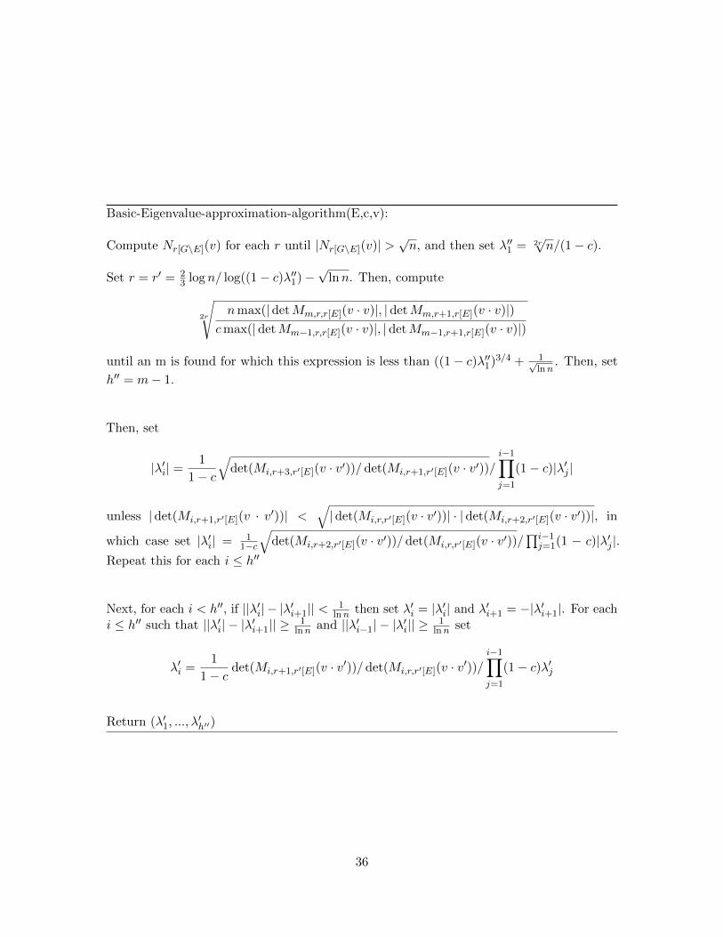
Basic-Eigenvalue-approximation-algorithm(E,c,v):

Compute Nr[G\E](v) for each r until |Nr[G\E](v)| >√n, and then set λ′′1 = 2r

√n/(1− c).

Set r = r′ = 23 log n/ log((1− c)λ′′1)−

√lnn. Then, compute

2r

√nmax(| detMm,r,r[E](v · v)|, | detMm,r+1,r[E](v · v)|)

cmax(|detMm−1,r,r[E](v · v)|, |detMm−1,r+1,r[E](v · v)|)

until an m is found for which this expression is less than ((1− c)λ′′1)3/4 + 1√lnn

. Then, set

h′′ = m− 1.

Then, set

|λ′i| =1

1− c

√det(Mi,r+3,r′[E](v · v′))/det(Mi,r+1,r′[E](v · v′))/

i−1∏j=1

(1− c)|λ′j |

unless | det(Mi,r+1,r′[E](v · v′))| <√| det(Mi,r,r′[E](v · v′))| · | det(Mi,r+2,r′[E](v · v′))|, in

which case set |λ′i| = 11−c

√det(Mi,r+2,r′[E](v · v′))/ det(Mi,r,r′[E](v · v′))/

∏i−1j=1(1 − c)|λ′j |.

Repeat this for each i ≤ h′′

Next, for each i < h′′, if ||λ′i| − |λ′i+1|| < 1lnn then set λ′i = |λ′i| and λ′i+1 = −|λ′i+1|. For each

i ≤ h′′ such that ||λ′i| − |λ′i+1|| ≥ 1lnn and ||λ′i−1| − |λ′i|| ≥ 1

lnn set

λ′i =1

1− cdet(Mi,r+1,r′[E](v · v′))/ det(Mi,r,r′[E](v · v′))/

i−1∏j=1

(1− c)λ′j

Return (λ′1, ..., λ′h′′)

36

Proof. If v is (23 · log n/ log((1− c)λ1, x)-good, there exists a constant r such that for any

r < r′′ < 23 · log n/ log((1− c)λ1),

min(P−1w)j4

((1− c)λ1)r′′

k∑j=1

wj ≤ |Nr′′[G\E](v[0])| ≤ ((1− c)λ1)r′′√

k((min pi)−1/2 + x)

So, the minimum r′′ such that |Nr′′[G\E](v)| >√n is within a constant of log n/2 log((1−c)λ1).

That means that |λ1 − λ′′1| is upper bounded by a constant multiple of 1/ log n, and thatr = r′ is within a constant of the value it would have if λ′′1 were λ1. This also implies that ifn is sufficiently large it is less than 2

3 · log n/ log((1− c)λ1)− 2h′ − 3.For m ≤ h′, r′′ ∈ r, r + 1, and v ∈ G if |λi| 6= |λi+1| then

|det(Mm,r′′,r′′[E](v · v))

γ((1−c)λj,m)cm

nm∏mi=1((1− c)λi)2r′′−2

√lnnwi(N√lnn[G\E](v)) ·Qwi(N√lnn[G\E](v))

−1| = o(1)

with probability 1− o(1). If |λi| = |λi+1| then λi = −λi+1, so either

γ((1− c)λm)2r−2√

lnnwm(N√lnn[G\E](v)) ·Qwm(N√lnn[G\E](v)) has the same sign as γ′((1−c)λm+1)2r−2

√lnnwm+1(N√lnn[G\E](v)) ·Qwm+1(N√lnn[G\E](v)) or

γ((1−c)λm)2r+1−2√

lnnwm(N√lnn[G\E](v))·Qwm(N√lnn[G\E](v)) has the same sign as γ′((1−c)λm+1)2r+1−2

√lnnwm+1(N√lnn[G\E](v)) ·Qwm+1(N√lnn[G\E](v))). Either way, we have that

(1− o(1))|γ((1− c)λj,m)cm

nm

m∏i=1

((1− c)λi)2r−2√

lnnwi(N√lnn[G\E](v)) ·Qwi(N√lnn[G\E](v))|

≤ max(|det(Mm,r,r[E](v · v))|, |det(Mm,r+1,r[E](v · v))|)

≤ (1 + o(1))| cm

nm

m−1∏i=1

((1− c)λi)2r+1−2√

lnnwi(N√lnn[G\E](v)) ·Qwi(N√lnn[G\E](v))|

· (|γ((1− c)λm)2r+1−2√

lnnwm(N√lnn[G\E](v)) ·Qwm(N√lnn[G\E](v))|

+ |γ′((1− c)λm+1)2r+1−2√

lnnwm+1(N√lnn[G\E](v)) ·Qwm+1(N√lnn[G\E](v))|)

with probability 1− o(1). Furthermore, by lemma 8, these bounds are within a factor ofO(ln2 n) of each other with probability 1− o(1).

That means that

nmax(| detMm,r,r[E](v · v)|, | detMm,r+1,r[E](v · v)|)cmax(| detMm−1,r,r[E](v · v)|, |detMm−1,r+1,r[E](v · v)|)

is within a factor of ln3(n) of |((1−c)λm)2r1−2√

lnnwm(N√lnn[G\E](v)) ·Qwm(N√lnn[G\E](v))|with probability 1− o(1), and thus that

2r1

√nmax(| detMm,r,r[E](v · v)|, |detMm,r+1,r[E](v · v)|)

cmax(| detMm−1,r,r[E](v · v)|, |detMm−1,r+1,r[E](v · v)|)= |(1− c)λm| ± o(1)

37

with probability 1− o(1). |(1− c)λm| ≥ 4√

(4(1− c)3λ31, so with probability 1− o(1), this

expression is not less than ((1− c)λ′′1)3/4 + 1√lnn

.

If m = h′ + 1, r′′ ∈ r, r + 1, and v ∈ G, then with probability 1 − o(1) either v is(r′′ + 2m+ 1, x)-bad or

|det(Mm,r,r′[E](v · v))|

≤ ch′+1

nh′+1ln2(n)(1− c)2h′·r′′

h′∏i=1

|λi|2r′′

(((1− c)λ1)2r′′

n+ ((1− c)λ1)r

′′/2

)· (1− c)r′′λr′′1

≤ 2ch′+1

nh′+1ln2(n)(1− c)2h′·r′′

h′∏i=1

|λi|2r′′ · ((1− c)λ1)3r′′/2

If v falls under the later case,

nmax(| detMm,r,r[E](v · v)|, | detMm,r+1,r[E](v · v)|)cmax(|detMm−1,r,r[E](v · v)|, |detMm−1,r+1,r[E](v · v)|)

= O(ln2(n)((1− c)λ1)3r/2)

, so

2r

√nmax(|detMm,r,r[E](v · v)|, |detMm,r+1,r[E](v · v)|)

cmax(|detMm−1,r,r[E](v · v)|, | detMm−1,r+1,r[E](v · v)|)= ((1−c)λ1)3/4+O(ln(ln(n))/ ln(n))

Therefore, with probability 1− o(1), either v is (23 · log n/ log((1− c)λ1), x)-bad or h′′ = h′.

By the previous two lemmas, with probability 1− o(1) either v is (r+ 2m+ 4, x)-bad, or

wi(N√lnn(v)) · P−1wi(N√lnn(v′))| ≥ λ2√

lnni / ln2 n

for all i ≤ h and

|det(Mm,r′′,r′[E](v · v′))

− cm

nm

m−1∏i=1

((1− c)λi)r′′+r′−2

√lnnwi(N√lnn[G\E](v)) ·Qwi(N√lnn[G\E](v

′))

· (γ((1− c)λm)r′′+r′−2

√lnnwm(N√lnn[G\E](v)) ·Qwm(N√lnn[G\E](v

′))

+ γ′((1− c)λm+1)r′′+r′−2

√lnnwm+1(N√lnn[G\E](v)) ·Qwm+1(N√lnn[G\E](v

′)))|

≤ 1

ln2m+2 n· c

m

nm

m∏i=1

|(1− c)λi|r′′+r′

for all m ≤ h′ + 1 and r ≤ r′′ < r + 4.Assume that the later holds. If |λm+1| < |λm| then if n is sufficiently large the γ′ term

will be negligable relative to the γ term, while if |λm+1| = |λm| increasing r′′ by two wouldmultiply both of these terms by (1− c)2λ2

m. Either way, we have that for any k ≤ h′ andr ≤ r′′ ≤ r + 1,

| det(Mm,r′′+2,r′[E](v · v′))/det(Mm,r′′,r′[E](v · v′))−k∏j=1

((1− c)λj)2| ≤ 1

ln7/8 n

38

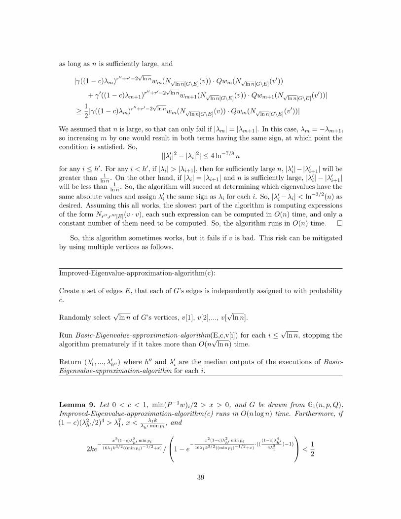
as long as n is sufficiently large, and

|γ((1− c)λm)r′′+r′−2


′))

+ γ′((1− c)λm+1)r′′+r′−2


′))|

≥ 1

2|γ((1− c)λm)r

′′+r′−2√

lnnwm(N√lnn[G\E](v)) ·Qwm(N√lnn[G\E](v′))|

We assumed that n is large, so that can only fail if |λm| = |λm+1|. In this case, λm = −λm+1,so increasing m by one would result in both terms having the same sign, at which point thecondition is satisfied. So,

||λ′i|2 − |λi|2| ≤ 4 ln−7/8 n

for any i ≤ h′. For any i < h′, if |λi| > |λi+1|, then for sufficiently large n, |λ′i|−|λ′i+1| will begreater than 1

lnn . On the other hand, if |λi| = |λi+1| and n is sufficiently large, |λ′i| − |λ′i+1|will be less than 1

lnn . So, the algorithm will suceed at determining which eigenvalues have the

same absolute values and assign λ′i the same sign as λi for each i. So, |λ′i−λi| < ln−3/2(n) asdesired. Assuming this all works, the slowest part of the algorithm is computing expressionsof the form Nr′′,r′′′[E](v · v), each such expression can be computed in O(n) time, and only aconstant number of them need to be computed. So, the algorithm runs in O(n) time.

So, this algorithm sometimes works, but it fails if v is bad. This risk can be mitigatedby using multiple vertices as follows.

Improved-Eigenvalue-approximation-algorithm(c):

Create a set of edges E, that each of G’s edges is independently assigned to with probabilityc.

Randomly select√

lnn of G’s vertices, v[1], v[2],..., v[√

lnn].

Run Basic-Eigenvalue-approximation-algorithm(E,c,v[i]) for each i ≤√

lnn, stopping thealgorithm prematurely if it takes more than O(n

√lnn) time.

Return (λ′1, ..., λ′h′′) where h′′ and λ′i are the median outputs of the executions of Basic-

Eigenvalue-approximation-algorithm for each i.

Lemma 9. Let 0 < c < 1, min(P−1w)i/2 > x > 0, and G be drawn from G1(n, p,Q).Improved-Eigenvalue-approximation-algorithm(c) runs in O(n log n) time. Furthermore, if(1− c)(λ2

h′/2)4 > λ71, x < λ1k

λh′ min pi, and

2ke−

x2(1−c)λ2h′ min pi

16λ1k3/2((min pi)

−1/2+x) /

1− e−


16λ1k3/2((min pi)

−1/2+x)·((

(1−c)λ4h′

4λ31)−1)

<1

2

39

then Improved-Eigenvalue-approximation-algorithm(c) returns (λ′1, ..., λ′h′′) such that h′ = h′′

and |λ′i − λi| < ln−3/2(n) for all i with probability 1− o(1).

Proof. Generating E takes O(n) time, picking v[i] takes o(n) time, each execution ofBasic-Eigenvalue-approximation-algorithm(c) runs in O(n

√log n) time, and combining their

outputs takes o(n) time. So, this algorithm runs in O(n log n) time.Assuming the conditions are satisfied, there exists y < 1

2 such that 1− y of G’s verticesare (2

3 · log n/ log((1− c)λ1, x)-good with probability 1− o(1). So, with probability 1− o(1),the majority of the selected vertices of G are (2

3 · log n/ log((1 − c)λ1), x)-good and themajority of the executions of Basic-Eigenvalue-approximation-algorithm give good output.If this happens, then the median value of h′′ is h′, and for each 1 ≤ i ≤ h′, the median valueof λ′i is within ln−3/2(n) of λi for each i, as desired.

Given approximations of PQ’s eigenvalues, one can attempt to approximate Ni(v) ·P−1Ni(v′) as follows.

Vertex-product-approximation-algorithm(v,v’,r,r’,E,c,(λ′1, ..., λ′h′′)):

(Assumes that Nr′′[G\E](v) has already been computed for r′′ ≤ r + 2h′′ + 3 and thatNr′′[G\E](v

′) has already been computed for r′′ ≤ r′)

For each i ≤ h′′, set

zi(v · v′) =det(Mi,r+1,r′[E](v · v′)− (1− c)iλ′i+1

∏i−1j=1 λ




·n(λ′i−1 − λ′i)γ((1− c)λ′j, i− 1)

cλ′i−1(λ′i − λ′i+1)γ((1− c)λ′j, i)((1− c)λ′i)−r−r

′−1

Return (z1(v · v′), ..., zh′′(v · v′)).

Lemma 10. Let 0 < c < 1, min(P−1w)i/2 > x > 0, G be drawn from G1(n, p,Q), E bea subset of G’s edges that independently contains each edge with probability c, v, v′ ∈ Gand

√lnn ≤ r′ ≤ r ∈ Z+, such that ((1 − c)λ2

h′/2)r+r′> λr+r

′

1 n. Also let (λ′1, ..., λ′h′′)

be a h′′-tuple which may depend on n such that h′′ = h′ and |λ′i − λi| ≤ ln−3/2(n) forall i. Assume that Nr′′[G\E](v) has already been computed for r′′ ≤ r + 2m + 3 andthat Nr′′[G\E](v

′) has already been computed for r′′ ≤ r′. Vertex-product-approximation-

algorithm(v, v′, r, r′, E, c, (λ′1, ..., λ′h′′)) runs in O(((1− c)λ1)r

′) average time. Furthermore,

with probability 1 − o(1), either v is (r + 2m + 4, x)-bad, v′ is (r′ + 1, x)-bad, or Vertex-product-approximation-algorithm(v, v′, r, r′, E, c, (λ′1, ..., λ

′h′′)) returns (z1(v · v′), ..., zh′(v · v′))

such that |zi(v · v′)− wi(v) · P−1wi(v′)| < 2x(min pj)−1/2 + x2 + o(1) for all i.

40

Proof. The slowest part of the algorithm is computing the expressions of the form Nr′′,r′[E](v ·v′). Each of these can be computed in O(E[|Nr′[G\E](v

′)|]) = O(((1− c)λ1)r′) average time,

and the number of these that need to be computed is constant in n. So, this algorithm runsin O(((1− c)λ1)r

′) average time.

With probability 1− o(1) either v is (r + 2m+ 4, x)-bad, v′ is (r′ + 1, x)-bad, or

wi(N√lnn(v)) · P−1wi(N√lnn(v′))| ≥ λ2√

lnni / ln2 n

for all i ≤ h and

|det(Mm,r′′,r′[E](v · v′))−cm

nm

m−1∏i=1

((1− c)λi)r′′+r′−2


′))

· (γ((1− c)λm)r′′+r′−2


′))

+ γ′((1− c)λm+1)r′′+r′−2


′)))|

≤ 1

ln2m+2 n· c

m

nm

m∏i=1

|(1− c)λi|r′′+r′

for all m ≤ h′ + 1 and r ≤ r′′ < r + 4.Assume that the later holds.

|det(Mi,r+1,r′[E](v · v′))− (1− c)iλ′i+1

i−1∏j=1

λ′j det(Mi,r,r′[E](v · v′))

− γλi − λi+1

λi· c

i

ni

i∏j=1

((1− c)λj)r+1+r′−2√

lnnwj(N√lnn[G\E](v)) ·Qwj(N√lnn[G\E](v′))|

≤ 1

lnn· | c

i

ni

i∏j=1

((1− c)λj)r+1+r′−2√

lnnwj(N√lnn[G\E](v)) ·Qwj(N√lnn[G\E](v′))|

for any i ≤ h with probability 1− o(1). So,

|det(Mi,r+1,r′[E](v · v′)− (1− c)iλ′i+1

∏i−1j=1 λ




− γ((1− c)λj, i)γ((1− c)λj, i− 1)

· λi−1(λi − λi+1)

λi(λi−1 − λi)

· cn

((1− c)λi)r+r′−2√

lnn+1wi(N√lnn[G\E](v)) ·Qwi(N√lnn[G\E](v′))|

≤ 1

n√

lnn· |((1− c)λi)r+r

′+1|

with probability 1− o(1). Therefore,

|zi(v · v′)− λ−1i ((1− c)λi)−2


′))| = o(1)

41

with probability 1− o(1). That implies that

|zi − wi(v) · P−1wi(v′)|

≤ |zi − (1− c)((1− c)λi)−2√

lnn−1wi(N√lnn[G\E](v)) ·Qwi(N√lnn[G\E](v′))|

+ (1− c) · |((1− c)λi)−2√

lnn−1wi(N√lnn[G\E](v)) ·Qwi(N√lnn[G\E](v′))

− ((1− c)λi)−√

lnn−1wi(v) ·Qwi(N√lnn[G\E](v′))|

+ |(1− c) · ((1− c)λi)−√

lnn−1wi(v) ·Qwi(N√lnn[G\E](v′))− wi(v) · P−1wi(v′))|

≤ |((1− c)λi)−√

lnnwi(N√lnn[G\E](v′)) · P−1[((1− c)λi)−

√lnnwi(N√lnn[G\E](v))− wi(v)]|

+ |wi(v) · P−1[((1− c)λi)−√

lnnwi(N√lnn[G\E](v′))− wi(v′)] + o(1)

By goodness of v and v′, this is less than or equal to

((1− c)λi)−√

lnn√wi(N√lnn[G\E](v

′)) · P−1wi(N√lnn[G\E](v′)) · x

+√wi(v) · P−1wi(v) · x+ o(1)

≤√wi(v′) · P−1wi(v′) + 2wi(v′) · P−1[((1− c)λi)−

√lnnwi(N√lnn[G\E](v

′))− wi(v′)]+

[((1− c)λi)−√

lnnwi(N√lnn[G\E](v′))− wi(v′)]

·P−1[((1− c)λi)−√

lnnwi(N√lnn[G\E](v′))− wi(v′)] · x

+ x√

1/min pj + o(1)

≤√

1/min pj + 2x/√

min pj + x2x+ x/√

min pj + o(1)

= (x2 + 2x(min pj)−1/2) + o(1)

with probability 1− o(1), as desired.

For any two vertices in different communities, v and v′, the fact that Q’s rows are distinct

implies that Q(−→v −

−−→v′) 6= 0. So, wi(v) 6= wi(v′) for some 1 ≤ i ≤ h′. That means

that for any two vertices v and v′,

(wi(v)− wi(v′)) · P−1(wi(v)− wi(v′))= wi(v) · P−1wi(v)− 2wi(v) · P−1wi(v′) + wi(v′) · P−1wi(v′) ≥ 0

for all 1 ≤ i ≤ h′, with equality for all i if and only if v and v′ are in the same community.This also implies that given a vertex v, another vertex in the same community v′, and avertex in a different community v′′,

2wi(v) · P−1wi(v′)− wi(v′) · P−1wi(v′)≥ 2wi(v) · P−1wi(v′′)− wi(v′′) · P−1wi(v′′)

for all 1 ≤ i ≤ h′ and the inequality is strict for at least one i. This suggests the followingalgorithms for classifying vertices.

42

Vertex-comparison-algorithm(v,v’, r,r’,E,x,c,(λ′1, ..., λ′h′′)):

(Assumes that Nr′′[G\E](v) and Nr′′[G\E](v′) have already been computed for r′′ ≤ r+2h′′+3)

Run Vertex-product-approximation-algorithm(v, v′, r, r′, E, c, (λ′1, ..., λ′h′′)), Vertex-product-

approximation-algorithm(v, v, r, r′, E, c, (λ′1, ..., λ′h′′)), and Vertex-product-approximation-

algorithm(v′, v′, r, r′, E, c, (λ′1, ..., λ′h′′)).

If ∃i : zi(v · v)− 2zi(v · v′) + zi(v′ · v′) > 5(2x(min pj)

−1/2 + x2) then conclude that v and v′

are in different communities.

Otherwise, conclude that v and v′ are in the same community.

Lemma 11. Assuming that each of G’s edges was independently assigned to E with prob-ability c, this algorithm runs in O(((1− c)λ1)max(r,r′)) average time. Furthermore, if eachexecution of Vertex-product-approximation-algorithm succeeds and 13(2x(min pj)

−1/2 + x2)is less than the minimum nonzero value of (wi(v)− wi(v′)) · P−1(wi(v)− wi(v′))then the algorithm returns the correct result with probability 1− o(1).

Proof. The slowest step of the algorithm is using Vertex-product-approximation-algorithm.This runs in an average time of O(((1− c)λ1)max(r,r′)) and must be done 3 times. If eachexecution of Vertex-product-approximation-algorithm succeeds then with probability 1− o(1)the zi are all within 6

5(2x(min pj)−1/2 + x2) of the products they seek to approximate, in

which casezi(v · v)− 2zi(v · v′) + zi(v

′ · v′) > 5(2x(min pj)−1/2 + x2)

if and only if(wi(v)− wi(v′)) · P−1(wi(v)− wi(v′)) 6= 0,

which is true for some i if and only if v and v′ are in different communities.

Vertex-classification-algorithm(v[],v’, r,r’,E,c,(λ′1, ..., λ′h′′)):

(Assumes that Nr′′[G\E](v[σ])have already been computed for 0 ≤ σ < k and r′′ ≤ r+2h′′+3,that Nr′′[G\E](v

′) has already been computed for all r′′ ≤ r′, and that zi(v[σ] · v[σ]) hasalready been computed for each i and σ)

Run Vertex-product-approximation-algorithm(v[σ], v′, r, r′, E, c, (λ′1, ..., λ′h′′)) for each σ.

Find a σ that minimizes the value of


zi(v[σ] · v[σ])− 2zi(v[σ] · v′)− [zi(v[σ′] · v[σ′])− 2zi(v[σ′] · v′)]

and conclude that v′ is in the same community as v[σ].

43

Lemma 12. Assuming that E was generated properly, this algorithm runs in O(((1−c)λ1)r′)

average time. Let x > 0 and assume that each execution of Vertex-product-approximation-algorithm succeeds (including the previous ones to compute zi(v[σ] · v[σ])), and that v[]contains exactly one vertex from each community. Also, assume that 13(2x(min pj)

−1/2 +x2)is less than the minimum nonzero value of (wi(v)− wi(v′)) · P−1(wi(v)− wi(v′)).Then this algorithm classifies v′ correctly with probability 1− o(1).

Proof. Again, the slowest step of the algorithm is running Vertex-product-approximation-algorithm. This runs in an average time of O(((1− c)λ1)r

′) and must be done k times. If

the conditions given above are satisifed, then each zi is within 2120(2x(min pj)

−1/2 + x2) ofthe product it seeks to approximate with probability 1− o(1). If this is the case, then

2wi(v′) · P−1wi(v[σ])− wi(v[σ]) · P−1wi(v[σ])≥ 2wi(v′) · P−1wi(v[σ′])− wi(v[σ′]) · P−1wi(v[σ′])

for all i and σ′ if v′ is in the same community as v[σ], and

2wi(v′) · P−1wi(v[σ])− wi(v[σ]) · P−1wi(v[σ])≤ 2wi(v′) · P−1wi(v[σ′])− wi(v[σ′]) · P−1wi(v[σ′])− 13(2x(min pj)

−1/2 + x2)

for some i and σ otherwise. So,

zi(v[σ] · v[σ])− 2zi(v[σ] · v′) ≤ zi(v[σ′] · v[σ])− 2zi(v[σ′] · v′) +19

3· (2x(min pj)

−1/2 + x2)

for all i and σ iff v′ is in the same community as v[σ]. So,


zi(v[σ]·v[σ])−2zi(v[σ]·v′)−[zi(v[σ′]·v[σ′])−2zi(v[σ′]·v′)] ≤ 19

3·(2x(min pj)

−1/2+x2)

iff v′ is in the same community as v[σ]. Therefore, the algorithm returns the correct resultwith probability 1− o(1).

At this point, we can finally start giving algorithms for classifying a graph’s vertices.

Lemma 13. Let x′ > 0, and assume that all of the following hold:

ε < 1

(1− c)λ4h′ > 4λ3

1

0 < x ≤ x′ < λ1k

λh′ min pi

(2(1− c)λ31/λ

2h′)

1−ε/3 < (1− c)λ1

(1 + ε/3) > log((1− c)λ1)/ log((1− c)λ2h′/2λ1)

13(2x′(min pj)−1/2 + (x′)2) < min

6=0(wi(v)− wi(v′)) · P−1(wi(v)− wi(v′))

∃k such that every entry of Qk is positive

∃w ∈ Rk such that QPw = λ1w,w · Pw = 1, and x ≤ minwi/2.

h′′ = h′

|λi − λ′i| ≤ ln−3/2(n) for all i

44

Unreliable-graph-classification-algorithm(G,c,m,ε,x,(λ′1, ..., λ′h′′)):

Randomly assign each edge in G to E independently with probability c.

Randomly select m vertices in G, v[0], ..., v[m− 1].

Let r = (1− ε3) log n/ log((1− c)λ′1)−

√lnn and r′ = 2ε

3 · log n/ log((1− c)λ′1)

Compute Nr′′[G\E](v[i]) for each r′′ ≤ r + 2h′′ + 3 and 0 ≤ i < m.

Run vertex-comparison-algorithm(v[i], v[j], r, r′, E, x, (λ′1, ..., λ′h′′)) for every i and j

If these give consistent results, randomly select one alleged member of each community v′[σ].Otherwise, fail.

For every v′′ in the graph, compute Nr′′[G\E](v′′) for each r′′ ≤ r′. Then, run

vertex-classification-algorithm(v′[], v′′, r, r′, E, (λ′1, ..., λ′h′′)) in order to get a hypothesized

classification of v′′

Return the resulting classification.

Let y = 2ke−


16λ1k3/2((min pi)

−1/2+x) /

1− e−


16λ1k3/2((min pi)

−1/2+x)·((

(1−c)λ4h′

4λ31)−1)

and y′ = 2ke

−x′2(1−c)λ2

h′ min pi

16λ1k3/2((min pi)

−1/2+x′) /

1− e−

x′2(1−c)λ2h′ min pi

16λ1k3/2((min pi)

−1/2+x′)·((

(1−c)λ4h′

4λ31)−1)

This algorithm runs in O(m2n1− ε

3 + n1+ 23ε) time. Furthermore, with probability 1− o(1),

G is such that Unreliable-graph-classification-algorithm(G, c,m, ε, x, (λ′1, ..., λ′h′′)) has at least

a1− k(1−min pi)

m −my

chance of classifying at least 1− y′ of G’s vertices correctly.

Proof. Let r0 = (1− ε3) log n/ log((1−c)λ1). There exists y′′ < y such that if these conditions

hold, then with probability 1− o(1), at least 1− y′′ of G’s vertices are (r0, x)-good and thenumber of vertices in G in community σ is within

√n log n of pσn for all σ. If this is the

case, then for sufficiently large n, it is at least 1− k(1−min pi)m −my likely that every one

of the m randomly selected vertices is (r0, x)-good and at least one is selected from eachcommunity.

If v[i] is (r0, x)-good for all i, then with probability 1 − o(1), vertex-comparison-algorithm(v[i], v[j], r, r′, E, x, c, (λ′1, ..., λ

′h′′)) determines whether or not v[i] and v[j] are

in the same community correctly for every i and j, allowing the algorithm to pick one mem-ber of each community. If that happens, then the algorithm will classify each (r′+h′, x′)-good

45

vertex correctly with probability 1−o(1). So, as long as the initial selection of v[] is good, thealgorithm classifies at least 1− y′ of the graph’s vertices correctly with probability 1− o(1).

Generating E and v[] takes O(n) time. Computing Nr′′[G\E](v[i]) for all r′′ ≤ r+ 2h′ + 3takes O(m| ∪r′′ Nr′′[G\E](v[i])) = O(mn) time, and computing Nr′′[G\E](v

′) for all r′′ ≤ r′

and v′ ∈ G takes

O(n| ∪r′′≤r′ Nr′′[G\E]) = O(n · ((1− c)λ1)r′) = O(n1+ 2

3ε)

time. Once these have been computed, running Vertex-comparison-algorithm(v[i], v[j], r, r′, E, x, (λ′1, ..., λ

′h′′)) for every i and j takes O(m2 · ((1 − c)λ1)r) =

O(m2n1− ε3 ) time, at which point an alleged member of each community can be found

in O(m2) time. Running Vertex-classification-algorithm(v′[], v′′, r, r′, E, c, (λ′1, ..., λ′h′′)) for

every v′′ ∈ G takes O(n · ((1− c)λ1)r′) = O(n1+ 2

3ε) time. So, the overall algorithm runs in

O(m2n1− ε3 + n1+ 2

3ε) average time.

So, this algorithm can sometimes give a vertex classification that is nontrivially betterthan that obtained by guessing. However, it has an assymptotically nonzero failure rateand requires too much information about the graph’s parameters. In order to get aroundthat, we combine the results of multiple executions of the algorithm and add in a parameteranalysis procedure as follows.

Lemma 14. Assume that there exist x, x′, and ε such that x is either a unit reciprocal or

46

Reliable-graph-classification-algorithm(G,m,δ, T(n)) (i.e., Agnostic-sphere-comparison):

Run Improved-Eigenvalue-approximation-algorithm(.1) in order to compute (λ′1, ..., λ′h′′)

Let λ′′1 = λ′1 + 2 ln−3/2(n), λ′′h′′ = λ′h′′ − 2 ln−3/2(n), and k′ = b1/δc

Let x be the smallest rational number of minimal numerator such that

k′(1− δ)m +m · 2k′e−

x2(λ′′h′′ )

2δ

16λ′′1 (k′)3/2((δ)−1/2+x) /

1− e−

x2(λ′′h′′ )

2δ

16λ′′1 (k′)3/2((δ)−1/2+x)·((

(λ′′h′′ )

4

4(λ′′1 )3)−1)

<1

2

Let ε be the smallest rational number of the form 1z or 1− 1

z such that (2(λ′′1)3/(λ′′h′′)2)1−ε/3 <

λ′′1 and (1 + ε/3) > log(λ′′1)/ log((λ′′h′′)2/2λ′′1)

Let c be the largest unit reciprocal less than 1/9 such that all of the following hold:

(1− c)(λ′′h′′)4 > 4(λ′′1)3

(2(1− c)(λ′′1)3/(λ′′h′)2)1−ε/3 < (1− c)λ′′1

(1 + ε/3) > log((1− c)λ′′1)/ log((1− c)(λ′′h′)2/2λ′′1)

k′(1− δ)m +m · 2k′e−

x2(1−c)(λ′′h′ )

2δ

16λ′′1 (k′)3/2((δ)−1/2+x) /

1− e−

x2(1−c)(λ′′h′′ )

2δ

16λ′′1 (k′)3/2((δ)−1/2+x)·((

(1−c)(λ′′h′′ )

4

4(λ′′1 )3)−1)

<1

2

Run Unreliable-graph-classification-algorithm(G, c,m, ε, x, (λ′1, ..., λ′h′′)) T (n) times and

record the resulting classifications.

Find the smallest y′′ such that there exists a set of more than half of the classificationsno two of which have more than y′′ disagreement, and discard all classifications not inthe set. In this step, define the disagreement between two classifications as the minimumdisagreement over all bijections between their communities.

For every vertex in G, randomly pick one of the remaining classifications and assert that it isin the community claimed by that classification, where a community from one classificationis assumed to correspond to the community it has the greatest overlap with in each otherclassification.

Return the resulting combined classification.

47

an integer, ε is a rational number of the form 1z or 1− 1

z , and all of the following hold:

2ke−

.9x2λ2h′ min pi

16λ1k3/2((min pi)

−1/2+x) /

1− e−

.9x2λ2h′ min pi

16λ1k3/2((min pi)

−1/2+x)·((

.9λ4h′

4λ31)−1)

<1

2

.9(λ2h′/2)4 > λ7

1

λ4h′ > 4λ3

1

0 < x ≤ x′ < λ1k

λh′ min pi

(2λ31/λ

2h′)

1−ε/3 < λ1

(1 + ε/3) > log(λ1)/ log(λ2h′/2λ1)

13(2x′(min pj)−1/2 + (x′)2) < min

6=0(wi(v)− wi(v′)) · P−1(wi(v)− wi(v′))

every entry of Qk is positive

∃w ∈ Rk such that QPw = λ1w,w · Pw = 1, and x ≤ minwi/2.

δ ≤ min pi

b1/δc · (1− δ)m +m · 2b1/δce−

x2λ2h′δ

16λ1b1/δc3/2(δ−1/2+x) /

1− e−

x2λ2h′δ

16λ1b1/δc3/2(δ−1/2+x)·((

λ4h′

4λ31)−1)

<1

2

T (n) = w(1)

T (n) ≤ ln(n)

min pi > 8ke−

.9x′2λ2h′ min pi

16λ1k3/2((min pi)

−1/2+x′) /

1− e−.9

x′2λ2h′ min pi

16λ1k3/2((min pi)

−1/2+x′)·((

.9λ4h′

4λ31)−1)

With probability 1− o(1), Reliable-graph-classification-algorithm(G,m,δ, T(n)) runs in

O(m2n1− ε3T (n) + n1+ 2

3εT (n)) time and classifies at least 1− 3y′ of G’s vertices correctly,

where

y′ = 2ke−

.9x′2λ2h′ min pi

16λ1k3/2((min pi)

−1/2+x′) /

1− e−.9

x′2λ2h′ min pi

16λ1k3/2((min pi)

−1/2+x′)·((

.9λ4h′

4λ31)−1)

Proof. With probability 1−o(1), Improved-Eigenvalue-approximation-algorithm gives outputsuch that h′′ = h′ and |λi − λ′i| ≤ ln−3/2(n) for each i. Assuming that this holds, thealgorithm finds the largest x and ε that satisfy the conditions above and the largest unitreciprocal less than 1/9, c, that satisifes the conditions for Unreliable-graph-classification-algorithm(G, c,m, ε, x, (λ′1, ..., λ

′h′′)) to have a greater than 1/2 success rate for any k ≤ b1/δc

with probability 1− o(1). Since its success rate is greater than 1/2 and T (n) = ω(1), morethan half of the executions of Unreliable-graph-classification-algorithm give classificationswith error y′ or less with probability 1− o(1). That means that y′′ ≤ 2y′ and at least oneof the classifications in the selected set must have error y′ or less. Thus, all of the selectedclassifications have error 3y′ or less. The requirement that min pi > 4y′ ensures that thebijection between any two of these classifications’ communities that minimizes disagreeement

48

is the identity. Therefore, this algorithm classifies at least 1− 3y′ of the vertices correctly,as desired.

Assuming this all works correctly, Improved-Eigenvalue-approximation-algorithm runsin O(n ln(n)) time. Finding x, ε, and c takes constant time, and running Unreliable-graph-

classification-algorithm T (n) times takes O(m2n1− ε3T (n) + n1+ 2

3εT (n)). Computing the

degree of agreement between each pair of classifications takes O(n ln2(n)) time. T (n) < lnn,so the brute force algorithm finds y′′ and the corresponding set in O(n) time. Combining theclassifications takes O(n) time. Therefore, this whole algorithm runs in O(m2n1− ε

3T (n) +

n1+ 23εT (n)) time with probability 1− o(1), as desired.

Proof of Theorem 6. If the conditions hold, Reliable-graph-classification-algorithm(G, ln(4b1/δc)/δ, δ, ln(n)) has the desired properties by the previous lemma.

7.2 Exact recovery

Recall that p is a probability vector of dimension k, Q is a k × k symmetric matrix withpositive entries, and G2(n, p,Q) denotes the stochastic block model with community priorp and connectivity matrix ln(n)Q/n. A random graph G drawn under G2(n, p,Q) has aplanted community assignment, which we denote by σ ∈ [k]n and call sometime the truecommunity assignment.

Recall also that exact recovery is solvable for a community partition [k] = tts=1As, ifthere exists an algorithm that assigns to each node in G an element of A1, . . . , At thatcontains its true community7 with probability 1 − on(1). Exact recovery is solvable inSBM(n, p,W ) if it is solvable for the partition of [k] into k singletons, i.e., all communitiescan be recovered.

7.2.1 Formal results

Definition 16. Let µ, ν be two positive measures on a discrete set X , i.e., two functionsfrom X to R+. We define the CH-divergence between µ and ν by

D+(µ, ν) := maxt∈[0,1]

∑x∈X

(tµ(x) + (1− t)ν(x)− µ(x)tν(x)1−t) . (16)

Note that for a fixed t,∑x∈X

(tµ(x) + (1− t)ν(x)− µ(x)tν(x)1−t)

is an f -divergence. For t = 1/2, i.e., the gap between the arithmetic and geometric means,we have ∑

x∈Xtµ(x) + (1− t)ν(x)− µ(x)tν(x)1−t =

1

2‖√µ−

√ν‖22 (17)

7Up to a relabelling of the communities.

49

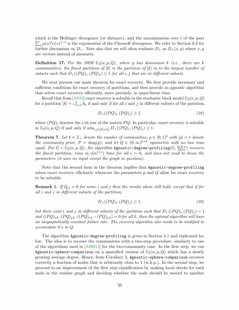
which is the Hellinger divergence (or distance), and the maximization over t of the part∑x µ(x)tν(x)1−t is the exponential of the Chernoff divergence. We refer to Section 8.3 for

further discussions on D+. Note also that we will often evaluate D+ as D+(x, y) where x, yare vectors instead of measures.

Definition 17. For the SBM G2(n, p,Q), where p has dimension k (i.e., there are kcommunities), the finest partition of [k] is the partition of [k] in to the largest number ofsubsets such that D+((PQ)i, (PQ)j) ≥ 1 for all i, j that are in different subsets.

We next present our main theorem for exact recovery. We first provide necessary andsufficient conditions for exact recovery of partitions, and then provide an agnostic algorithmthat solves exact recovery efficiently, more precisely, in quasi-linear time.

Recall that from [AS15] exact recovery is solvable in the stochastic block model G2(n, p,Q)for a partition [k] = tts=1As if and only if for all i and j in different subsets of the partition,

D+((PQ)i, (PQ)j) ≥ 1, (18)

where (PQ)i denotes the i-th row of the matrix PQ. In particular, exact recovery is solvablein G2(n, p,Q) if and only if mini,j∈[k],i 6=j D+((PQ)i, (PQ)j) ≥ 1.

Theorem 7. Let k ∈ Z+ denote the number of communities, p ∈ (0, 1)k with |p| = 1 denotethe community prior, P = diag(p), and let Q ∈ (0,∞)k×k symmetric with no two rowsequal. For G ∼ G2(n, p,Q), the algorithm Agnostic-degree-profiling(G, ln lnn

4 lnn ) recoversthe finest partition, runs in o(n1+ε) time for all ε > 0, and does not need to know theparameters (it uses no input except the graph in question).

Note that the second item in the theorem implies that Agnostic-degree-profiling

solves exact recovery efficiently whenever the parameters p and Q allow for exact recoveryto be solvable.

Remark 1. If Qij = 0 for some i and j then the results above still hold, except that if forall i and j in different subsets of the partition,

D+((PQ)i, (PQ)j) ≥ 1, (19)

but there exist i and j in different subsets of the partition such that D+((PQ)i, (PQ)j) = 1and ((PQ)i,k ·(PQ)j,k ·((PQ)i,k−(PQ)j,k) = 0 for all k, then the optimal algorithm will havean assymptotically constant failure rate. The recovery algorithm also needs to be modified toaccomodate 0’s in Q.

The algorithm Agnostic-degree-profiling is given in Section 3.1 and replicated be-low. The idea is to recover the communities with a two-step procedure, similarly to oneof the algorithms used in [ABH14] for the two-community case. In the first step, we runAgnostic-sphere-comparison on a sparsified version of G2(n, p,Q) which has a slowlygrowing average degree. Hence, from Corollary 2, Agnostic-sphere-comparison recoverscorrectly a fraction of nodes that is arbitrarily close to 1 (w.h.p.). In the second step, weproceed to an improvement of the first step classification by making local checks for eachnode in the residue graph and deciding whether the node should be moved to another

50

community or not. This step requires solving a hypothesis testing problem for deciding thelocal degree profile of vertices in the SBM. The CH-divergence appears when resolving thisproblem, as the mis-classification error exponent. We present this result of self-interest inSection 7.2.2. The proof of Theorem 7 is given in Section 7.2.3.

Agnostic-degree-profiling algorithm.Inputs: a graph G = ([n], E), and a splitting parameter γ ∈ [0, 1] (see Theorem 7 for thechoice of γ).Output: Each node v ∈ [n] is assigned a community-list A(v) ∈ A1, . . . , At, whereA1, . . . , At is intended to be the partition of [k] in to the largest number of subsets such thatD+((pQ)i, (pQ)j) ≥ 1 for all i, j in [k] that are in different subsets.Algorithm:(1) Define the graph G′ on the vertex set [n] by selecting each edge in G independently withprobability γ, and define the graph G′′ that contains the edges in G that are not in G′.(2) Run Agnostic-sphere-comparison on G′ to obtain the preliminary classification σ′ ∈[k]n (see Section 7.1 and Corollary 2.)(3) Estimate p and Q based on the alleged communities’ sizes and the edge densities betweenthem.(4) For each node v ∈ [n], determine in which community node v is most likely to belong tobased on its degree profile computed from the preliminary classification σ′ and the estimatesof p and Q (see Section 7.2.2), and call it σ′′v(5) Re-estimate p and Q based on the sizes of the communities claimed by σ′′ and the edgedensities between them.(6) For each node v ∈ [n], determine in which group A1, . . . , At node v is most likely tobelong to based on its degree profile computed from the preliminary classification σ′′ andthe new estimates of P and Q (see Section 7.2.2).

7.2.2 Testing degree profiles

In this section, we consider the problem of deciding which community a node in the SBMbelongs to based on its degree profile. The notions are the same as in [AS15], we repeat themto ease the reading and explain how the Agnostic-degree-profiling algorithm works.

Definition 18. The degree profile of a node v ∈ [n] for a partition of the graph’s verticesinto k communities is the vector d(v) ∈ Zk+, where the j-th component dj(v) counts thenumber of edges between v and the vertices in community j. Note that d(v) is equal to N1(v)as defined in Definition 8.

For G ∼ G2(n, p,Q), community i ∈ [k] has a relative size that concentrates exponentiallyfast to pi. Hence, for a node v in community j, d(v) is approximately given by

∑i∈[k]Xijei,

where Xij are independent and distributed as Bin(npi, ln(n)Qi,j/n), and where Bin(a, b)denotes8 the binomial distribution with a trials and success probability b. Moreover, theBinomial is well-enough approximated by a Poisson distribution of the same mean in this

8Bin(a, b) refers to Bin(bac, b) if a is not an integer.

51

regime. In particular, Le Cam’s inequality gives∥∥∥∥Bin

(na,

ln(n)

nb

)− P (ab ln(n))

∥∥∥∥TV

≤ 2ab2 ln2(n)

n, (20)

hence, by the additivity of Poisson distribution and the triangular inequality,

‖µd(v) − P(ln(n)∑i∈[k]

piQi,jei)‖TV = O

(ln2(n)

n

). (21)

We will rely on a simple one-sided bound (see (44)) to approximate our events under thePoisson measure.

Consider now the following problem. Let G be drawn under the G2(n, p,Q) SBM andassume that the planted partition is revealed except for a given vertex. Based on the degreeprofile of that vertex, is it possible to classify the vertex correctly with high probability?We have to resolve a hypothesis testing problem, which involves multivariate Poisson distri-butions in view of the previous observations. We next study this problem.

Testing multivariate Poisson distributions. Consider the following Bayesian hy-pothesis testing problem with k hypotheses. The random variable H takes values in [k] withPH = j = pj (this is the a priori distribution of H). Under H = j, an observed randomvariable D is drawn from a multivariate Poisson distribution with mean λ(j) ∈ Rk+, i.e.,

PD = d|H = j = Pλ(j)(d), d ∈ Zk+, (22)

where

Pλ(j)(d) =∏i∈[k]

Pλi(j)(di), (23)

and

Pλi(j)(di) =λi(j)

di

di!e−λi(j). (24)

In other words, D has independent Poisson entries with different means. We use the followingnotation to summarize the above setting:

D|H = j ∼ P(λ(j)), j ∈ [k]. (25)

Our goal is to infer the value of H by observing a realization of D. To minimize the errorprobability given a realization of D, we must pick the most likely hypothesis conditioned onthis realization, i.e.,

argmaxj∈[k]PD = d|H = jpj , (26)

which is the Maximum A Posteriori (MAP) decoding rule.9 To resolve this maximization,we can proceed to a tournament of k − 1 pairwise comparisons of the hypotheses. Eachcomparison allows us to eliminate one candidate for the maxima, i.e.,

PD = d|H = ipi > PD = d|H = jpj ⇒ H 6= j. (27)

9Ties can be broken arbitrarily.

52

The error probability Pe of this decoding rule is then given by,

Pe =∑i∈[k]

PD ∈ Bad(i)|H = ipi, (28)

where Bad(i) is the region in Zk+ where i is not maximizing (26). Moreover, for any i ∈ [k],

PD ∈ Bad(i)|H = i ≤∑j 6=i

PD ∈ Badj(i)|H = i (29)

where Badj(i) is the region in Zk+ where PD = x|H = ipi ≤ PD = x|H = jpj . Notethat with this upper-bound, we are counting the overlap regions where PD = x|H = ipi ≤PD = x|H = jpj for different j’s multiple times, but no more than k − 1 times. Hence,∑

j 6=iPD ∈ Badj(i)|H = i ≤ (k − 1)PD ∈ Bad(i)|H = i. (30)

Putting (28) and (29) together, we have

Pe ≤∑i 6=j

PD ∈ Badj(i)|H = ipi, (31)

=∑i<j

∑d∈Zk+

min(PD = d|H = ipi,PD = d|H = jpj) (32)

and from (30),

Pe ≥1

k − 1

∑i<j

∑d∈Zk+

min(PD = d|H = ipi,PD = d|H = jpj). (33)

Therefore the error probability Pe can be controlled by estimating the terms∑

d∈Zk+min(PD =

d|H = ipi,PD = d|H = jpj). In our case, recall that

PD = d|H = i = Pλ(i)(d), (34)

which is a multivariate Poisson distribution. In particular, we are interested in the regimewhere k is constant and λ(i) = ln(n)ci, ci ∈ Rk+, and n diverges. Due to (32), (33), wecan then control the error probability by controlling

∑x∈Zk+

min(Pln(n)ci(x)pi,Pln(n)cj (x)pj),

which we will want to be o(1/n) to classify vertices in the SBM correctly with high probabilitybased on their degree profiles (see next section). The following lemma provides the relevantestimates.

Lemma 15. For any c1, c2 ∈ (R+ \ 0)k with c1 6= c2 and p1, p2 ∈ R+ \ 0,∑x∈Zk+

min(Pln(n)c1(x)p1,Pln(n)c2(x)p2) = O

(n−D+(c1,c2)− ln ln(n)

2 ln(n)

), (35)

∑x∈Zk+

min(Pln(n)c1(x)p1,Pln(n)c2(x)p2) = Ω

(n−D+(c1,c2)− k ln ln(n)

2 ln(n)

), (36)

where D+(c1, c2) is the CH-divergence as defined in (16).

53

In other words, the CH-divergence provides the error exponent for deciding amongmultivariate Poisson distributions. We did not find this result in the literature, but founda similar result obtained by Verdu [Ver86], who shows that the Hellinger distance (thespecial case with t = 1/2 instead of the maximization over t) appears in the error exponentfor testing Poisson point-processes, although [Ver86] does not investigate the exact errorexponent. This lemma was proven in [AS15].

This lemma together with previous bounds on Pe imply that if D+(ci, cj) > 1 for alli 6= j, the true hypothesis is correctly recovered with probability o(1/n). However, it may bethat D+(ci, cj) > 1 only for a subset of (i, j)-pairs. What can we then infer? While we maynot recover the true value of H with probability o(1/n), we may narrow down the searchwithin a subset of possible hypotheses with that probability of error.

Testing composite multivariate Poisson distributions. We now consider theprevious setting, but we are no longer interested in determining the true hypothesis, butin deciding between two (or more) disjoint subsets of hypotheses. Under hypothesis 1, thedistribution of D belongs to a set of possible distributions, namely P(λi) where i ∈ A, andunder hypothesis 2, the distribution of D belongs to another set of distributions, namelyP(λi) where i ∈ B. Note that A and B are disjoint subsets such that A ∪B = [k]. In short,

D|H = 1 ∼ P(λi), for some i ∈ A, (37)

D|H = 2 ∼ P(λi), for some i ∈ B, (38)

and as before the prior on λi is pi. To minimize the probability of deciding the wronghypothesis upon observing a realization of D, we must pick the hypothesis which leads tothe larger probability between PH ∈ A|D = d and PH ∈ B|D = d, or equivalently,∑

i∈APλ(i)(d)pi ≥

∑i∈BPλ(i)(d)pi ⇒ H = 1, (39)∑

i∈APλ(i)(d)pi <

∑i∈BPλ(i)(d)pi ⇒ H = 2. (40)

In other words, the problem is similar to the previous one, using the above mixturedistributions. If we denote by Pe the probability of making an error with this test, we have

Pe =∑x∈Zk+

min

(∑i∈APλ(i)(x)pi,

∑i∈BPλ(i)(x)pi

). (41)

Moreover, applying bounds on the minima of two sums,

Pe ≤∑x∈Zk+

∑i∈A,j∈B

min(Pλ(i)(x)pi,Pλ(j)(x)pj

), (42)

Pe ≥1

|A||B|∑x∈Zk+

∑i∈A,j∈B

min(Pλ(i)(x)pi,Pλ(j).(x)pj

). (43)

Therefore, for constant k and λ(i) = ln(n)ci, ci ∈ Rk+, with n diverging, it suffices to controlthe decay of

∑x∈Zk+

min(Pλ(i)(x)pi,Pλ(j)(x)pj) when i ∈ A and j ∈ B, in order to bound

54

the error probability of deciding whether a vertex degree profile belongs to a group ofcommunities or not.

The same reasoning can be applied to the problem of deciding whether a given nodebelongs to a group of communities, with more than two groups. Also, for any p and p′ suchthat |pj − p′j | < lnn/

√n for each j, Q, γ(n), and i,

∑x∈Zk+

max

(Bin(

np′, (1−γ(n)) ln(n)n

Qi

)(x)− 2PPQi(1−γ(n)) ln(n)/n(x), 0

)= O(1/n2). (44)

So, the error rate for any algorithm that classifies vertices based on their degree profile in agraph drawn from a sparse SBM is at most O(1/n2) more than twice what it would be ifthe probability distribution of degree profiles really was the poisson distribution.

In summary, we have proved the following.

Lemma 16. Let k ∈ Z+ and let A1, . . . , At be disjoint subsets of [k] such that ∪ti=1Ai = [k].Let G be a random graph drawn under G2(n, p, (1 − γ(n))Q). Assigning the most likelycommunity subset Ai to a node v based on its degree profile d(v) gives the correct assignmentwith probability

1−O(n−(1−γ(n))∆− 1

2ln((1−γ(n)) lnn)/ lnn +

1

n2

),

where

∆ = minr,s∈[t]r 6=s

mini∈Ar,j∈As

D+((pQ)i, (pQ)j). (45)

Moreover, in order to prove Theorem 7, we will need a version of this lemma thatstill holds when some of our information is inaccurate. First of all, consider attemptingthe previous testing procedure when one thinks the distributions are λ′ with probabilityp′ instead of λ with probability p. Assume that there exists ε such that for all i and j,|λ′(i)j−λ(i)j | ≤ εmin(λ′(i)j , λ(i)j) and |p′i−pi| ≤ εmin(p′i, pi). Then for any i ∈ A, x ∈ Zk+,the previous hypothesis testing procedure will not classify x as being in B unless∑

j∈B(1 + ε)|x|+1Pλ(j)(x)pj ≥ (1 + ε)−|x|−1Pλ(i)(x)pi

That means that for any i ∈ A, x ∈ Zk+, the probability that x arises from Pλ(i) and is thenmisclassified as being in B is at most

Pλ(i)(x)pi ≤∑j∈B

(1 + ε)2|x|+2Pλ(j)(x)pj

So, this hypothesis testing procedure has an error probability of at most∑x∈Zk+

(1 + ε)2|x|+2∑

i∈A,j∈Bmin

(Pλ(i)(x)pi,Pλ(j)(x)pj

)Furthermore,

55

Lemma 17. For any p and Q there exists c such that the following holds for all δ < min pi/2.Let G be a random graph drawn from G2(n, p,Q), and σ′ be a classification of G’s verticesthat misclassifies δn vertices. Also, let p′ be the frequencies with which vertices are classifiedas being in the communities, and Q′ be n/ lnn times the edge densities between the allegedcommunities. Then with probability 1−o(1), every element of p′ or Q′ is within cδ+

√lnn/n

of the corresponding element of p or Q.

Proof. With probability 1 − o(1), the size of every community is within√

lnn/n of itsexpected value, and the edge density between each pair of communities is within

√n lnn

of its expected value. Also, there exists a constant c′ such that with probability 1− o(1),no vertex has degree more than c′ lnn. Assuming this is the case, the misclassification ofvertices can not change the apparent number of edges between any two communities bymore than c′δn lnn, and it can not change the apparent size of any community by morethan δn. Thus, |p′i − pi| ≤

√lnn/n+ δ and

|Q′i,j −Qi,j | ≤√

lnn/n+ 4c′δ

pi · pj+ 4Qi,j

δpi + δpj + δ2

pipj

This lets us prove the following “robust” version of this lemma to prove Theorem 7.

Lemma 18. Let k ∈ Z+ and let A1, . . . , At be disjoint subsets of [k] such that ∪ti=1Ai = [k].Let G be a random graph drawn under G2(n, p, (1 − γ(n))Q). There exist c1, c2, and c3

such that with probability 1− o(1) G is such that for any sufficiently small δ, assigning themost likely community subset Ai to a node v based on a distortion of its degree profile thatindependently gets each node’s community wrong with probability at most δ and estimates ofp and Q based on a classification of the graphs vertices that misclassifies each vertex withprobability δ gives the correct assignment with probability at least

1− c2 · (1 + c1δ)c3 lnn ·

(n−(1−γ(n))∆− 1

2ln((1−γ(n)) lnn)/ lnn

)− c2

n2,

where

∆ = minr,s∈[t]r 6=s

mini∈Ar,j∈As

D+((pQ)i, (pQ)j). (46)

Proof. First, note that by the previous lemma, with probability 1 − o(1), G is such thatevery element of the estimates of p and Q is within cδ +

√lnn/n of its true value. Choose

c3 such that every vertex in the graph has degree less than c3 lnn with probability 1− o(1).If this holds, then the probability of misclassifying a vertex based on its true degree profileand the estimates of its parameters is at most

2(1 + 2cδ/min(pi, (PQ)i,j))2c3 lnn+2 ·

(n−(1−γ(n))∆− 1

2ln((1−γ(n)) lnn)/ lnn

)+O

(1

n2

)based on the previous bounds on the probability that classifying a vertex based on its degreeprofile fails.

56

Now, let

c′1 = maxi,j

∑pi′qi′,j/(piqi,j).

The key observation is that v’s mth neighbor had at least a mini,j(piqi,j)/∑pi′qi′,j chance

of actually being in community σ for each σ, so its probability of being reported as being incommunity σ is at most 1 + c′1δ times the probability that it actually is. So, the probabilitythat its reported degree profile is bad is at most (1 + c′1δ)

|N1(v)| times the probability thatits actual degree profile is bad. The conclusion follows.

7.2.3 Proof of Theorem 7

We prove the possibility result here. The converse was proven in [AS15] for known parame-ters, hence also applies here.

Let G ∼ G2(n, p,Q) and γ = ln lnn4 lnn , and A1, . . . , At be a partition of [k]. Agnostic-degree-

profiling(G, p,Q, γ) recovers the partition [k] = tts=1As with probability 1− on(1) if forall i, j in [k] that are in different subsets,

D+((PQ)i, (PQ)j) ≥ 1. (47)

The idea behind Claim 1 is contained in Lemma 16. However, there are several technicalsteps that need to be handled:

1. The graphs G′ and G′′ obtained in step 1 of the algorithm are correlated, since anedge cannot be both in G′ and G′′. However, this effect can be discarded since twoindependent versions would share edges with low enough probability.

2. The classification in step 2 using Agnostic-sphere-comparison has a vanishingfraction of vertices which are wrongly labeled, and the SBM parameters are unknown.This requires using the robust version of Lemma 16, namely Lemma 18.

3. In the case where D+((PQ)i, (PQ)j) = 1 a more careful classification is needed ascarried in steps 3 and 4 of the algorithm.

Proof. With probability 1−O(1/n), no vertex in the graph has degree greater than c3 lnn.Assuming that this holds, no vertex’s set of neighbors in G′′ is more than

(1−max qi,j lnn/n)−c3 lnn · (n/(n− c3 lnn))c3 lnn = 1 + o(1)

times as likely to occur as it would be if G′′ were independent of G′. So, the fact that theyare not has negligible impact on the algorithm’s error rate. Now, let

δ = (e(1−γ)2c3

mini6=j D+((PQ)i,(PQ)j) − 1)/c1.

By Lemma 18, if the classification in step 2 has an error rate of at most δ, then theclassification in step 3 has an error rate of

O(n−(1−γ) mini 6=j D+((PQ)i,(PQ)j)/2 + 1/n2),

57

observing that if σ′v 6= σv the error rate of σ′′v′ for v′ adjacent to v is at worst multiplied by aconstant. That in turn ensures that the final classification has an error rate of at most

O

((1 +O(n−(1−γ) mini 6=j D+((PQ)i,(PQ)j)/2 + 1/n2))c3 lnn 1

nlnn−1/4

)= O

(1

nlnn−1/4

).

58

recovering communities in the general stochastic block model without ... · recovering communities...

Documents