reconstruction of a tornado disaster employing remote ... · reconstruction of a tornado disaster...
TRANSCRIPT

i
Reconstruction of a Tornado Disaster Employing Remote Sensing Techniques: A
Case Study of the 1999 Moore, Oklahoma Tornado
by
Melissa A. Wagner
A Thesis Presented in Partial Fulfillmentof the Requirements for the Degree
Masters of Arts
Approved April 2011 by theGraduate Supervisory Committee:
Randall S. Cerveny, Co-ChairSoe W. Myint, Co-Chair
Elizabeth A. WentzAnthony J. Brazel
ARIZONA STATE UNIVERSITY
May 2011

ii
ABSTRACT
Remote sensing has demonstrated to be an instrumental tool in monitoring
land changes as a result of anthropogenic change or natural disasters. Most
disaster studies have focused on large-scale events with few analyzing small-scale
disasters such as tornadoes. These studies have only provided a damage
assessment perspective with the continued need to assess reconstruction. This
study attempts to fill that void by examining recovery from the 1999 Moore,
Oklahoma Tornado utilizing Landsat TM and ETM+ imagery. Recovery was
assessed for 2000, 2001 and 2002 using spectral enhancements (vegetative and
urban indices and a combination of the two), a recovery index and different
statistical thresholds. Classification accuracy assessments were performed to
determine the precision of recovery and select the best results. This analysis
proved that medium resolution imagery could be used in conjunction with
geospatial techniques to capture recovery. The new indices, Shortwave Infrared
Index (SWIRI) and Coupled Vegetation and Urban Index (CVUI), developed for
disaster management, were the most effective at discerning reconstruction using
the 1.5 standard deviation threshold. Recovery rates for F-scale damages revealed
that the most incredibly damaged areas associated with an F5 rating were the
slowest to recover, while the lesser damaged areas associated with F1-F3 ratings
were the quickest to rebuild. These findings were consistent for 2000, 2001 and
2002 also exposing that complete recovery was never attained in any of the F-
scale damage zones by 2002. This study illustrates the significance the
biophysical impact has on recovery as well as the effectiveness of using medium
resolution imagery such as Landsat in future research.

iii
ACKNOWLEDGEMENTS
I would like to thank the following people: Kimme DeBiasse for
formatting help, Barbara Trapido-Lurie for helping me beautify my maps and
tailor the information to my audience, Shai Kaplan for bouncing remote sensing
ideas off of, and Chris Galetti for atmospheric correction and the use of his
labtop; only crisp and beautiful images from now on. I am extremely fortunate to
Dr. Brazel who took an interest in my application and offered sage advice. Thank
you Dr. Elizabeth Wentz, for letting me camp out during your class to work on
my research, your poignant insights and support, and believing in me. While I
know I tried the patience of Dr. Soe Myint, I am forever indebted to you for my
remote sensing education, introduction to tornado damage assessment and
brilliant guidance in my research. To Dr. Randall Cerveny, may I never hear the
phrase “If it was easy, everybody would do it.” Thank you for letting me be the
headstrong, obstinate student I am, but most importantly for never giving up on
me and coaxing me along the way when I seriously doubted my abilities. My best
friends, Kym Suthers, Heidi Berardi and Tracy Schirmang for their support,
editing capabilities including untangling the words in my head and
encouragement to pursue my passion regardless of the difficulty. To my children,
Paix, Cierra, Hugo and Helen, follow your dreams, live passionately and never set
limits. Education will take you wherever you envision yourselves. Lastly, but
most importantly, my husband, Joe Wagner, without your support none of this
would be possible and understanding this is only the beginning.

iv
TABLE OF CONTENTS
Page
LIST OF TABLES..................................................................................... vi
LIST OF FIGURES .................................................................................. vii
1. INTRODUCTION .................................................................................. 1
1.1 Introduction............................................................................... 1
1.2 Research Question .................................................................... 2
1.3 Background .............................................................................. 5
1.4 Framework ............................................................................... 6
2. LITERATURE REVIEW ....................................................................... 8
2.1 Theory of Hazards..................................................................... 8
2.2 Damage Assessment ............................................................... 17
2.3 Aerial photography ................................................................. 21
2.4 Remote Sensing ...................................................................... 22
2.5 Conclusion .............................................................................. 30
3. STUDY, DATA AND METHODS ...................................................... 32
3.1 Introduction............................................................................. 32
3.2 Study Area .............................................................................. 32
3.3. Data and Data Preparation ..................................................... 35
3.4. Digital Analysis ..................................................................... 39

v
3.5 Change Vector Analysis ......................................................... 46
3.6 Conclusion .............................................................................. 47
4. RESULTS ............................................................................................. 49
4.1 Introduction............................................................................. 49
4.2 Assessment of New Indices and Initial Impact of Tornado.... 49
4.3 Performance of the Recovery Index ....................................... 55
4.4 Annual Reconstruction and Recovery Rates........................... 69
4.5 Recovery Rates as a Function of the Fujita Scale................... 76
4.6 Change Vector Analysis ......................................................... 84
4.7 Conclusion .............................................................................. 84
5. DISCUSSION....................................................................................... 86
5.1 Introduction............................................................................. 86
5.2 Remotely Sensed Data and Recovery Index........................... 87
5.3 Recovery Rates as a Function of F-scale ................................ 92
5.4 Conclusion .............................................................................. 97
6. SUMMARY AND CONCLUSION ..................................................... 99
6.1 Summary................................................................................. 99
6.2 Suggestions for Future Research .......................................... 100
6.3 Significance........................................................................... 101
REFERENCES ....................................................................................... 103

vi
LIST OF TABLESTable Page
1. Specific satellite imagery utilized in the study ..................................... 36
2. List of Threshold Values of 0.5, 1.0, 1.5 standard deviations to define
recovery for each index and year. ................................................. 45
3. Sampled Means of Different Land Cover Classes. ............................... 50
4. Accuracy Assessments listed by Index, Standard Deviation Threshold
and Year. ....................................................................................... 66
5. Averaged Accuracy Assessments listed by Index and Standard
Deviation Threshold. (Overall = Overall accuracy, Prod. =
Producer’s accuracy, User’s = User’s Accuracy) ......................... 67
6. Annual Recovery Rates listed by Index, Threshold (Thres.) and Year. 71
7. Recovery Rates for F-scale zones listed by Index, Threshold (Thres.)
and Year. ....................................................................................... 78
8.Recovery Rates for F-scale zones listed by Index, Threshold and Year 79
9. List of Land Class Types and Associated Land Use Changes.............. 82
vii
LIST OF FIGURES
Figure Page
Fig. 1. Map of recorded tornado locations during the May 3, 1999
Tornado Outbreak in Central Oklahoma....................................... 35
Fig. 2. Map displaying county boundaries in the state of Oklahoma and the
study area outlined in red.............................................................. 38
Fig. 3. False Color Composite of the Study Area displaying Band 4 in red,
Band 3 in green and Band 2 in blue. ............................................. 38
Fig. 4. 1998 Urban Index showing the transect of different land covers of
the 1999 Moore, Oklahoma Tornado-impacted region a year before
the tornado disaster. ...................................................................... 50
Fig. 5. Reflectance Curves for Coupled Vegetation and Urban Index,
Normalized Difference Vegetative Index, Soil Adjusted Vegetative
Index, Shortwave Infrared Index, Urban Index.. .......................... 51
Fig. 6. 1999 Coupled Vegetation and Urban Image (CVUI) of the Moore,
Oklahoma Tornado-impacted region. ........................................... 52
Fig. 7. 1999 Urban Index (UI) of the Moore, Oklahoma Tornado-impacted
region. ........................................................................................... 53
Fig. 8. 1999 Normalized Difference Vegetative Index (NDVI) of the
Moore, Oklahoma Tornado-impacted region. .............................. 53
Fig. 9. 1999 Soil Adjusted Vegetative Index (SAVI) for the Moore,
Oklahoma Tornado-impacted region. ........................................... 54

viii
Figure Page
Fig. 10. 1999 Shortwave Infrared Vegetative Index (SWIRI) for the
Moore, Oklahoma Tornado-impacted region. .............................. 54
Fig. 11. 1999 Urban Index showing the transect for 1999 Moore,
Oklahoma Tornado-impacted region right after the tornado
disaster. ......................................................................................... 55
Fig. 12. Transect of Damaged Area affected by the 1999 Moore,
Oklahoma 4.3................................................................................ 55
Fig. 13. 2000 Recovery Image of Coupled Vegetation and Urban Image
CVUI of the 1999 Moore, Oklahoma Tornado-impacted region. 57
Fig. 14. 2001 Recovery Image of Coupled Vegetation and Urban Image
CVUI of the 1999 Moore, Oklahoma Tornado-impacted region. 58
Fig. 15. 2002 Recovery Image of Coupled Vegetation and Urban Image
CVUI of the 1999 Moore, Oklahoma Tornado-impacted region. 58
Fig.16. 2000 Recovery Image of the Urban Index (UI) of the 1999 Moore,
Oklahoma Tornado-impacted region. ........................................... 59
Fig. 17. 2001 Recovery Image of the Urban Index (UI) of the 1999 Moore,
Oklahoma Tornado-impacted region. ........................................... 59
Fig.18. 2002 Recovery Image of the Urban Index (UI) of the 1999 Moore,
Oklahoma Tornado-impacted region. ........................................... 60
Fig. 19. 2000 Recovery Image of Normalized Difference Vegetative Index
(NDVI) of the 1999 Moore, Oklahoma Tornado-region. ............. 60

ix
Figure Page
Fig. 20. 2001 Recovery Image of Normalized Difference Vegetative Index
(NDVI) of the 1999 Moore, Oklahoma Tornado-impacted region.
....................................................................................................... 61
Fig. 21. 2002 Recovery Image of Normalized Difference Vegetative Index
(NDVI) of the 1999 Moore, Oklahoma Tornado-impacted region.
....................................................................................................... 61
Fig. 22. 2000 Recovery image of Soil Adjusted Vegetative Index (SAVI)
of the 1999 Moore, Oklahoma Tornado-impacted region. ........... 62
Fig . 23. 2001 Recovery image of Soil Adjusted Vegetative Index (SAVI)
of the 1999 Moore, Oklahoma Tornado-impacted region. ........... 62
Fig. 24. 2002 Recovery image of Soil Adjusted Vegetative Index (SAVI)
of the 1999 Moore, Oklahoma Tornado-impacted region. ........... 63
Fig. 25. 2000 Recovery image of the Shortwave Infrared Index (SWIRI)
of the 1999 Moore, Oklahoma tornado-impacted region.............. 63
Fig. 26. 2001 Recovery image of the Shortwave Infrared Index (SWIRI)
of the 1999 Moore, Oklahoma tornado-impacted region.............. 64
Fig.27. 2002 Recovery image of the Shortwave Infrared Index (SWIRI) of
the 1999 Moore, Oklahoma tornado-impacted region.................. 64
Fig. 28. Map of the 1999 impacted region showing recovered and
damaged regions for 2000, 2001 and 2002 using the Coupled
vegetative and urban index and 1.0 standard deviation threshold. 72
x
Figure Page
Fig. 29. Map of the 1999 impacted region showing recovered and
damaged regions for 2000, 2001 and 2002 using the coupled
vegetative and urban index and 1.5 standard deviation threshold. 73
Fig. 30. Map of the 1999 impacted region showing recovered and
damaged regions for 2000, 2001 and 2002 using the Shortwave
Infrared Index (SWIRI) and 1.0 standard deviation threshold. .... 73
Fig. 31. Map of the 1999 impacted region showing recovered and
damaged regions for 2000, 2001 and 2002 using the Shortwave
Infrared Index (SWIRI) and 1.5 standard deviation threshold. .... 74
Fig. 32. Map of the 1999 Moore Oklahoma Tornado-impacted region
showing recovered and damaged regions for 2000, 2001 and 2002
using the Urban Index (UI) and 1.0 standard deviation threshold.75
Fig. 33. Map of the 1999 Moore Oklahoma Tornado-impacted region
showing recovered and damaged regions for 2000, 2001 and 2002
using the Urban Index (UI) and 1.5 standard deviation threshold.75
Fig. 34. Graph for the 1999 Moore Oklahoma Tornado-impacted region
displaying annual recovery rates for 2000, 2001 and 2002 in
percent by F-scale intensity as established by the recovery index.80
Fig. 35. Graph for the 1999 Moore Oklahoma Tornado-impacted region
displaying F-scale recovery rates in percent for 2000, 2001 and
2002 as established by the recovery index.................................... 81
xi
Figure Page
Fig. 36. Change Vector Analysis Map of the 1999 Moore Oklahoma
Tornado-impacted region for 2000 showing different land class
changes.......................................................................................... 82
Fig. 37. Map of the 1999 Moore Oklahoma Tornado-impacted region
showing the magnitude of changes for 2000 using change vector
analysis.......................................................................................... 83
Fig. 38. Map of the 1999 Moore Oklahoma Tornado-impacted region
showing the magnitude of changes for 2001 using change vector
analysis.......................................................................................... 84
Fig. 39. Map of the 1999 Moore Oklahoma Tornado-impacted region
showing the magnitude of changes for 2002 using change vector
analysis.......................................................................................... 84
1
1. Introduction
1.1 Introduction
Hazard studies have recognized remote sensing technology as a powerful
tool in damage assessment and recovery analysis. These methods have been
extensively used in monitoring land cover changes resulting from natural and
anthropogenic processes as a result of its ubiquitous coverage, regular data
collection and repeatable independent analyses (Magsig et al. 2000, Yuan et al.
2002, Myint et al. 2008, Myint et al. 2008b, Mura et al. 2008). Through the
manipulation of multispectral data, damaged areas can be detected by the
alterations of spectral signatures in land cover features caused by a natural
disaster (Bentley et al. 2002, Yuan et al. 2002, Jedlovec et al. 2006). Depending
on the technology selection and resolution employed, different damage levels can
be discerned, thus serving as a low cost alternative to aerial photography or
intensive ground surveys (Yuan et al. 2002, Jedlovec et al. 2006, Myint et al.
2008, Myint et al. 2008b).
Improvements in resolution and image processing techniques have
recently made remote sensing an increasingly popular method for studying
disaster impacts (Yuan et al. 2002). Finer resolutions have improved the
discernment of small-scale features; yet, drawbacks exist as the result of more
intensive algorithms and increasing processing times for imagery analysis. While
detailed damage information can be obtained on individual objects with finer
resolution, this imagery may fail to capture the extent of the impacted areas due to
much smaller scenes. Medium resolution imagery such as Landsat TM and

2
Landsat ETM+ considers ground features together with the bigger pixel size,
thereby providing a top-view assessment. With the development of an effective
series of image processing algorithms, this imagery could better capture the
chaotic nature of damaged areas than fine resolution imagery.
Most disaster studies have focused on issues of vulnerability and recovery
with large-scale events such as floods, earthquakes, tsunamis and hurricanes.
While tornado damage may be viewed as only affecting a small concentrated area,
there is still a need to examine the impacts tornadoes have on society. Depending
on the intensity of the tornado and the infrastructure within its path, the magnitude
of damage can actually be greater than large-scale events.
Understanding all aspects of a disaster from its impact to recovery is
crucial in implementing effective mitigation strategies for future events (Uitto
1998, Cutter 2003). More recently, issues of social vulnerabilities and recovery
have been brought to the forefront with such notable disasters as the December
2004 Tsunami, Hurricane Katrina and Haitian Earthquake. While these factors
affect society’s ability to recover, the scope and magnitude of the disaster still
plays a critical role in societal recovery and resiliency (Cutter 1996, Cutter et al.
2003). Examining disparities in reconstruction due to the biophysical impact can
provide valuable information in the degree of restoration and recovery. This
knowledge would lead to better decision-making policies that could reduce
disparities in the reconstruction process within the most severely damaged areas.
1.2 Research Question

3
Hazard studies have shown that the effects of a natural disaster to a society
are not uniform. The scope and magnitude of the disaster can have a lasting
impact based on the amount of damage sustained, thus affecting the ability to
fully recover (Dacy and Kunreuther 1969, Haas et al. 1977, Uitto 1998, Yasui
2007, Fitch et al. 2010, Aldridge 2011). Most disaster studies have assessed the
initial damages and reconstruction of large-scale events like hurricanes,
earthquakes and tsunamis, but very few hazard studies have examined the lasting
impacts of small-scale events like tornadoes.
Remote sensing techniques have more recently been employed in the few
tornado disaster studies. Their research (Magsig et al. 2000, Yuan et al. 2002,
Jedlovec et al. 2006, Myint et al. 2008, Wilkinson and Crosby 2010) only
examined the initial impact with regards to the extent and severity of damages.
Another study by Myint et al 2008b expanded on previous damage studies by
categorizing the different F-scale ratings through geospatial techniques.
However, no known study has employed geospatial methods as a means to
objectively capture the reconstruction of a tornado disaster.
This study attempts to answer the following research questions:
How effective are geospatial techniques in assessing recovery and
reconstruction using medium resolution imagery (e.g. Landsat TM or
Landsat ETM+)?
Are recovery rates uniform with regard to damage level (e.g., Fujita
scale)?

4
These questions can be addressed through a study involving remote
sensing and GIS technologies. My hypothesis is that recovery rates are directly
dependent on the level of the damage sustained, as measured by the Fujita Scale.
Consequently, employing an analysis involving geospatial techniques will assess
the initial tornado damage and reconstruction using Landsat-TM and Landsat
ETM+ imagery before and several years after the disaster.
This analysis focuses on the 1999 Moore, Oklahoma tornado event of May
3, 1999. The tornado first touched down in the central portion of Grady County
and traveled 38 miles before dissipating on the eastern side of Oklahoma City in
Oklahoma County. Within the path, the cities of Moore and Bridge Creek
sustained the most damage based on its dense infrastructure and inferred intensity
rating of F5 on the Fujita Scale. The impact of the 1999 Moore, Oklahoma
tornado was 36 people lost their lives and damages exceeded 1.6 billion US
dollars making it one of the costliest tornadoes in US history (Brooks and
Doswell 2002, NCDC 2010).
For the Moore, Oklahoma tornado, image-processing techniques were
performed on Landsat TM imagery of 1998, 1999, 2000, 2001, and 2002. These
images were normalized the data to reduce spatial and temporal variations not
associated with the tornado (Singh 1989, Myint et al. 2008). Spectral
enhancements and temporal differencing were also employed to discern changes
attributed to the tornado. Both damaged and recovered areas were classified
using a recovery index and spatially analyzed in conjunction with F-scale zones

5
determined by National Weather Service ground surveys. Recovery rates were
then computed for each F-scale zone.
By examining the recovery rate of the Moore, Oklahoma tornado, the
hypothesis is that the response to such a disaster is not uniform, but rather a
function of the biophysical impact. By revealing these issues of disparity, future
studies can use this knowledge to implement better planning methods and
mitigation strategies in the most impacted regions that can be expected to reduce
the recovery period for those groups most impacted by the storm.
1.3 Background
After a tornado event, damage surveys are conducted to assess the extent
of the damaged area and classify the intensity of the tornado on the Fujita Scale.
Since no direct measurements can be made, the intensity of the tornado must be
inferred by correlating the level of damage and estimated wind speeds (Marshall
2002, McDonald 2002, Doswell et al. 2009). Ratings on this scale range from F0
to F5 where an F5 rating corresponds to the most incredible degree of damage
(Fujita 1971, 1981, 1993, Grazulis 1991). Recently, this scale was modified to
reduce the subjectivity of the scale and renamed to the Enhanced Fujita Scale with
EF ratings (McDonald 2002). However, this change was made several years after
the tornado, therefore, I used the classified tornado ratings in the context of the
original Fujita Scale.
To research recovery, remote sensing methods of spectral enhancements,
temporal differencing and series of image processing algorithms were used.
Spectral enhancements can discern damages not readily visible to the human eye

6
either by either reducing data redundancy (e.g. principle components analysis
(PCA)) or algebraically manipulating bands (e.g. band ratioing) on a single image.
Temporal differencing differs from spectral enhancements in a new image is
produced based on the subtraction two images of the same area to highlight
changed areas (Singh 1989, Myint et al. 2008). With these images, a series of
image processing techniques were employed to classify damaged and recovered
regions using a recovery index and different thresholds. The top-performing
results were spatially analyzed in conjunction with F-scale damage zones to
derive F-scale recovery rates for the specific recovery years of 2000, 2001, and
2002.
1.4 Framework
To accomplish this geospatial assessment of the reconstruction of the 1999
Moore, Oklahoma Tornado, my thesis is organized as follows:
Chapter 2 provides a detailed literature review on issues pertaining to both
hazards and remote sensing components. This section is divided into discussions
of biophysical and social vulnerability factors concerning the initial impacts and
the recovery process. This chapter also examines previous remote sensing studies
for both large-scale events and small-scale events with regards to damage
assessments and recovery analysis. By reviewing both hazard perspectives and
geospatial techniques, this section aims to produce a comprehensive view of the
recovery process after a natural disaster.
Chapter 3 discusses the study area, data selected for the analysis, and
methods involved in assessing reconstruction. Limitations inherent in the data
7
and quality control methods necessary for successful change detection are
addressed. Geospatial techniques for analyzing the reconstruction process are
discussed as well as how recovery rates were calculated.
In Chapter 4, the results produced from the methods are presented.
Detected changes in terms of damaged and recovered regions are discussed. Both
recovery rates and spatial disparities are analyzed and presented.
In Chapter 5, the results from Chapter 4 are interpreted with the key
findings discussed. Critical findings regarding geospatial assessments of the
reconstruction of a tornado and spatial disparities are explained.
In Chapter 6, the key findings are summarized and fundamental
conclusions of this thesis are offered. Suggestions for future work are highlighted
with the significance of this work closing this research.
8
2. Literature Review
2.1 Theory of Hazards
When a natural process or phenomenon negatively impacts society, that
event concentrated in time and space is labeled a natural disaster (Turner 1976,
Alexander 1991). Unlike a disaster, a natural hazard is the perceived threat or
likelihood of loss from a future occurrence of suffering an adverse effect where
human vulnerability intersects with the biophysical processes (Fussel 2007). At
this intersection, the impacts of a disaster can either be attenuated or amplified
depending on the type of implemented mitigation strategies and underlining social
characteristics (Alexander 1991, Cutter 2003, Turner et al. 2003, Cutter 2008).
Understanding how the biophysical process integrates with the socio-environment
is crucial in not only measuring the sensitivity of the impact, but also in
determining the recovery and resiliency of the region (Cutter 1996).
The emergence of hazard studies in geography began with Barrows (1923)
by taking an ecological approach to human adaptation and the environment
(Alexander 1991). He analyzed spatial and temporal aspects of risk and
susceptibility, but only focused on high magnitude events. Brookfield (1964)
pointed out contradictions with perceptions and responses to hazards calling to
expand the scope of how it relates to the socio-environment system (Grossman
1977, Alexander 1991). Following Brookfield, Hewitt and Burton (1971)
recognized human elements in disasters in addition to geophysical components
(Cutter et al. 2003). Further research by Burton et al. 1978 stressed viewing
hazards as ongoing phenomena within socio-environment systems, thus

9
advancing hazards research beyond causal agents. Building on this ecological
perspective, Timmerman (1981) argued that disasters were largely functions of
societal vulnerabilities in terms of sensitivity and resiliency of a system (Cutter
1996, Adger 2006, Fussel 2007).
Hazard research can be broken down into aspects of vulnerability and
resiliency (Klein et al 2003, Adger 2006, Zhou et al. 2010). Vulnerability broadly
defined is the potential for loss (Cutter 1996, Cutter et al 2003, Etkin et al. 2004,
Berkes et al. 2005) and can be further subdivided into physical and social
components. Physical vulnerability, or risk, is the likelihood of experiencing
some adverse effect based on the geophysical characteristics of the environment,
whereas, social vulnerability is concerned with whom or what is susceptible to the
loss (Turner 1976, Turner et al. 2003, Cutter et al 2003; 2008). Resiliency, unlike
risk and social vulnerability, is concerned with post-event impacts and measures
how an individual or group responds and recovers once the disaster has occurred
(Cutter 1996, Turner et al. 2003, Cutter et al. 2008).
In hazard studies, risk loosely defined is the likelihood of the phenomena
occurring with an undesirable outcome (Brooks et al. 2003). From the beginning
of hazard research, risk has been viewed as the distribution from some hazard
condition (Burton et al. 1978, Alexander 1991, Cutter 1996). Here, inhabiting in
hazard zones and the degree of loss is associated with a regionalized event based
on known past occurrences (Cutter 1996, Brooks et al. 2003). Within these zones,
risk can either be attenuated or amplified depending on the magnitude, duration,

10
impact and onset of the event as well as any mitigation strategies already in place
(Cutter 1996, Mileti 1999, Mitchell 1999, Uitto 1999, Cutter et al. 2008).
Social vulnerability like risk is also concerned with the antecedent
conditions of the event except the focus shifts from the physical characteristics of
the hazard to social concerns in terms of whom or what is exposed to the loss
(Turner 1976, Turner et al. 2003, Cutter et al. 2003; 2008). This concept views
the hazard draped over society as a given and investigates who or what would be
most adversely affected based on social conditions (Cutter et al. 2003; 2008).
Here, disadvantaged groups are more vulnerable to certain hazards based on lower
socioeconomic means, lack of resources and poor housing quality regardless of
the distance to the damaging source (Burton et al. 1993, Cutter 2000). The
disparaging impacts of a disaster can be attributed to social inequalities based on
factors of age, race, ethnicity, socioeconomic status, political institutions and
other social variables (Liverman 1990, Burton et al. 1993, Blaikie et al 1994,
Cutter 1996; 2000, Cutter et al. 2003). Recent examples of these inequalities have
been noted with the impact and recovery of Hurricane Katrina and the 2004
Tsunami (Finch et al. 2010)
In addition to the aforementioned factors, social vulnerability takes into
account how the built environment is constructed from a generalized paradigm.
This aspect of social vulnerability has essentially evolved from engineering
mitigation strategies that have recognized shortcomings in dwelling types, certain
types of infrastructure, and urban versus rural settings. Certain dwelling types
and infrastructure have proven to be a key factor in disaster impacts based on

11
material composition and number of housing units within a dwelling as shown by
Uitto 1998, Mitchell 1999 and Mileti 1999. In particular, mobile homes and
manufacturing houses are far more susceptible to damage than the typical framed
house even when anchored to a foundation (Marshal 2002, Pan 2002). While
these dwellings only make up about 8% of the housing market, approximately
40% of the tornado fatalities occur in these structures (Simmons 2007). These
marginalized residents comprised of elderly and low-income families are 10 to 15
times more likely to die in a tornado disaster than the occupants of a single family
framed home (Brooks and Doswell 2002, Simmons 2007).
Urban settings can also compound the effects of a disaster due to higher
density and societal trends. Higher densities in the urban environment increase the
conditional risk for fatalities by generating more debris and consequently
projectiles (Brooks and Doswell 2002, Marshall 2002, Pan 2002, DeSilva et al.
2008). This produces a domino effect in damage patterns and can often lead to
structural failure of surrounding structures in wind driven disasters and flooding
events (Brooks and Doswell 2002, Marshall 2002, Pan 2002, Brooks et al. 2003,
DeSilva et al. 2008). In the case of tornado disasters, both structural failures and
wind-driven projectiles are responsible for the leading cause of death (Brooks and
Doswell 2000, Boruff et al. 2003).
Societal trends in urban settings also pose a higher risk based on growing
populations. With an increased demand for housing and service buildings, rushed
decision making in planning and construction could affect the integrity of the
structure and consequently increase the building’s vulnerability (Uitto 1998,

12
Marshall 2002, Brooks et al. 2003, Cutter 2003, Doswell 2005, Cutter et. al 2008,
Wentz et al. 2009). The presence of such vulnerable structures within this
environment could compromise the integrity of nearby buildings, thereby
producing a larger damage field (Uitto 1998, Marshall 2002, Brooks et al. 2003,
Cutter 2003, Doswell 2005, Cutter et. al 2008, DeSilva et al. 2008, Wentz et al.
2009). However, rural settings could just as vulnerable as the urban environment
due to the lack of building code enforcement necessary to ensure their structural
integrity despite their sparse spacing (Cross 2001, Cutter 2003).
Another social vulnerability factor that should be considered is hazard
perception. (Preston et al. 1983, Alexander 1991, Donner 2007). Due to
variations within society, perception differences arise based on levels of interest
and the ability to implement protective measures (Donner 2007). How this threat
is perceived affects their anticipated responses and consequently the magnitude of
the impact (Preston et al. 1983, Alexander 1991, Cutter 1996, Donner 2007).
Additionally, perception in terms of public apathy contributes to be a major factor
in how prepared a society is due to long intervals between high magnitude events
or frequent exposure to low impact events that become integrated within the
culture (Preston et al 1983, Alexander 1991, Cutter 1996, Brooks and Doswell
1998; 2002, Doswell 2005). Perceived psychological distances and imagined
boundaries drawn around the threat can also foster a false sense of security,
thereby affecting the level of preparedness and consequently the degree of impact
(Davis 2003).

13
Another aspect that has been evolving over recent years is place-based
vulnerabilities. This dimension of vulnerability fuses the biophysical and social
factors together to examine the most vulnerable subgroups within a geographic
region (Liverman 1990, Cutter 1996). Certain places or sites can exhibit higher
degrees of vulnerability based on the spatial clustering of social and biophysical
characteristics (Cutter et al. 2000). This paradigm seeks not only to understand
the local manifestation of vulnerability, but also the influence of larger factors
operating on bigger scales (Cutter 1996, Cutter et al. 2000, Turner et al. 2003,
Cutter et al. 2008). As a result, this view has moved hazard studies away from the
fragmented or specialized approach common in the local or regional level to a
more integrative approach (Blaikie and Brookfield 1987, Wilhite and Easterling
1987, Mitchell et al. 1989, Lewis 1987; 1990, Liverman 1990, Degg 1993,
Longhurst 1995, Cutter 1996).
In addition to vulnerability, another core aspect studied in hazard research
is resiliency. This concept measures how well a system can handle stress by
focusing on the post-disaster responses and coping capacities of individuals or
groups (Cutter 1996, Turner et. al 2003, Cutter et. al 2008, Zhou et al. 2010). As
noted by Cutter et al. 2008, “Resiliency incorporates the capacity to reduce or
avoid losses, contain the effects of disasters, and recover with minimal social
disruptions” (Buckle et al. 2000, Manyena 2006, Tierney and Bruneau 2007,
Cutter et al. 2008, p 600). This concept considers both pre-disaster mitigation and
post-disaster strategies with the notion that a well-designed and resourceful
system can handle the external stresses of an event and still maintain its integrity

14
(Adger 1997, Klein et al. 2003, Bruneau et al. 2003, Berkes et al. 2005, Tierney
and Bruneau 2007, Cutter et al. 2008).
The relationship between resiliency and vulnerability has been argued
within the discipline based on how resiliency is conceptualized. Traditionally,
hazard studies have nested resiliency within vulnerability based on defining
resiliency as an outcome or coping mechanism to the disaster (Cutter 1996).
Other researchers, more in lined with socio-ecologists, treat vulnerability and
resiliency as separate and opposite concepts (Turner et al. 2003). With this
paradigm, resiliency is treated as a process by which a system modifies and copes
with the aftermath based on adaptive capacities and knowledge gained (Cutter et
al. 2008, Zhou et al. 2010). The last paradigm does not discriminate between
resiliency as a process or outcome, but instead links these two concepts through a
dynamical feedback with the ideology that a more resilient society will be less
vulnerable and vice versa (Cutter 1996). While this conceptualization has been
growing in popularity, problems exist in both measuring and delineating between
these core aspects (Cutter et al. 2008).
Issues in assessing vulnerability and resiliency also exist when dealing
with spatial and temporal components. In terms of scale, attributes selected to
measure a particular variable may not always transcend across other scales
without losing some detailed information (Turner et al. 2003). In regards to
temporal aspects, the true onset of an event may be difficult to define depending
on measurement unit and scale (Turner et al. 2003, Cutter et al. 2008). In addition
to identifying the impact, the declaration of recovery can be somewhat ambiguous
15
as other factors or outside scale influences can affect the reconstruction process
(Cutter et al. 2008).
After the disaster has occurred, there are two generalized phases within the
disaster management cycle. The first phase deals with the initial consequences of
the disaster in terms of emergency responses including rescues, evacuations,
temporary shelters and damage assessments (Alexander 2000, Carter 1991,
Quarantelli 1998, Dunford and Li 2011). The second phase, recovery,
incorporates both short-term reconstruction and long-term planning. The short-
term reconstruction consists of repairing and rebuilding damaged housing and
infrastructure that could last up to three years, while long-term recovery pertains
to economic development and long-term mitigation plans (Alexander 2000, Carter
1991, Quarantelli 1998, Dunford and Li 2011). Ideally, these two recovery
concepts should overlap in the rebuilding phase to improve the resiliency of the
impacted society from future events (Burby 2001).
Focusing on short-term recovery, reconstruction rates depend on the
magnitude of the biophysical impact as well as social vulnerability factors. Dacy
and Kunreuther (1969) initially noted that the rate of recovery was mainly
attributed to the magnitude of damage sustained in the recovery assessment of the
1964 Alaskan earthquake (Haas et al. 1977, Yasui 2007, Fitch et al. 2010,
Aldridge 2011). Both Haas et al. 1977 and Yasui 2007 elaborated on this finding
by pointing out that the lesser damaged structures will take less time and
resources to complete (Aldridge 2011). They continued to state that the most
severely damaged areas will lag in reconstruction due to more resources necessary

16
for either intricate repairs or complete rebuilds as well as issues of shorter housing
supplies for temporary residence (Aldridge 2011). This finding was demonstrated
in an economic assessment by Desilva et al. 2004, which inferred recovery based
on property values returning to pre-tornado disaster prices in Oklahoma County.
They found that the housing prices associated with the most incredibly damaged
ranking of an F5 lagged the market prices of less damaged homes before finally
rebounding three years later. This illustrates the significance that the magnitude of
the biophysical impact has on the rate of recovery (Cutter 1996; 2000; 2003, Fitch
et al. 2010).
Within short-term reconstruction, another indirect ramification of the
impact to consider is the decision to rebuild or relocate. This decision is
predominantly based on the loss of livelihood and income opportunities or fear of
another event (Paul 2005). In a study by Paul 2005, he examined the connection
between aid and outmigration in of a tornado disaster in north-central Bangladesh.
Through mail surveys and interviews, he discovered that all residents stayed
based on receiving more aid than anticipated. However, he did point out that the
generous amount of aid was in response to a previous tornado disaster in this
region that had generated negatively publicity based on government negligence.
Contrary to this finding, another study by Cross 2001 revealed that only half of
the population returned to the rural community of Spencer, Kansas, Cross (2001)
based on mail surveys without mentioning of aid amounts. His study focused
more on the rural versus urban argument in which small town livelihoods played a
crucial role in the decision to remain and rebuild.

17
2.2 Damage Assessment
Once a tornado has occurred, damage surveys are conducted to determine
the inferred intensity of the tornado and extent of its path. From these surveys,
the tornado is assigned an F-scale rating on the Fujita Scale based on correlating
inferred wind speeds from the observed degrees of damages (Fujita 1971, 1981,
Fujita and Smith 1993, McDonald 2002, Marshall 2002). All observed tornadoes
have been assigned an F-scale rating since the implementation of the Fujita Scale
in the 1970s and continues to be the most requested statistic following a tornado
disaster to date (Grazulis 1991, McCarthy 2003).
Although the Fujita scale is meant to be an intensity scale, this scale is
really more of a damage scale (Doswell and Burgess 1988). F-scale ratings
implicitly equate damage with intensity primarily based on its interception with
the constructed environment (Doswell and Burgess 1988, Brooks 2003, Doswell
et al. 2003, Dotzek et al. 2003). Significant tornado ratings, F3 or higher, are
often assigned only when tornadoes initiate construction failure and scatter debris
over large expanses (Doswell et al. 2003, Dotzek et al. 2003). In relatively
remote locations, tornadoes that are observed are usually assigned much lower
ratings because their paths often traverse vegetative cover with little chance to
intersect infrastructure. Although tornadoes in densely populated regions are
more likely to be reported with higher damage ratings, other difficulties exists in
rating F-0 tornadoes based on small damage amounts and brief lifetimes (Brooks
2003, Dotzek et al. 2003). These aforementioned problems highlight the issue of
the dependency of F-scale ratings with the underline material and not solely on

18
inferred wind speeds, which this scale aims to achieve (Doswell and Burgess
1988, Doswell et al. 2009).
Additional problems with the Fujita Scale result from the subjective nature
in damage assessments and other underline assumptions. When surveying
tornado damage, a great deal of uncertainty exists with the interpretation of the
single paragraph descriptors that are often deemed vague and limited in scope
(Grazulis 1991, Marshall 2002). These biases are often exacerbated based on the
knowledge of different estimators, which can lead to spatial and temporal
inconsistencies in rating tornadoes (Doswell et al. 2009). Other discrepancies can
be attributed to the assumption of well-built structures and their homogeneous
construction instead of the considering the construction the variability of
construction (Marshall 2002, Doswell et al. 2009). As a result, these problems
and inconsistencies can affect the completeness and accuracy of tornado
climatology (McCarthy 2003, Doswell et al. 2009).
Some of these issues were addressed with the modification of the Fujita
Scale to develop the Enhanced Fujita Scale. Adjustments included more detailed
damage descriptors to reduce subjectivity in damage surveys and account for
construction variability and building types (Doswell et al. 2009). Additional
damage indicators were also implemented to deal with damages to different types
of vegetation (Doswell et al. 2009). However, these indicators still fail to
represent the various vegetation types as well as capture any of the antecedent
conditions in terms of soil saturation that may contribute to damage severity. In
addition to the improved damage descriptors, wind speed ranges were also

19
lowered based on the observation of building failure initiation at much lower
speeds than previous thought (Doswell et al. 2009). Yet, despite these
modifications, problems still remain due to the inherent subjectivity in damage
surveys and dependency of intercepting structures necessary to infer tornadic
intensity with wind speeds.
Despite the aforementioned issues in the Fujita Scale, relating damage to
intensity can be useful in modeling hazards associated with tornadoes (Schaefer et
al. 2002, McCarthy 2003). Since implementing the Fujita Scale, damaged
surveys have noted the different magnitudes of observed damages based on rough
guidelines built in the scale (Doswell and Burgess 1988). Upon surveying
different damage swaths, weaker structures were more susceptible to wind
damage based on materials and poor construction practices (Marshall 2002).
Within the past decade, damage surveys have brought forth new information on
the correlation of structural engineering and quality to observed damages.
In particular, detailed surveys of the Moore, Oklahoma tornado made
important discoveries concerning the relationship between architectural design
and degrees of damage. Roof attachment and geometry were found to contribute
to the magnitude of damage as the result of weight distribution and number of
connections (Brooks and Doswell 2002, Marshall 2002). These results were
important findings considering structural failure is often initiated when uneven
pressure fields expose these connections. Garage doors also posed a higher risk
for greater damage since positive wind pressure can easily raise these relatively
flimsy doors (Marshall 2002, Brooks and Doswell 2002). This breach of
20
envelope creates additional pressure side loads that can cause the roof to uplift
and often initiates structural failure (Marshall 2002).
In addition to the direct impacts of the tornado itself, indirect impacts such
as projectiles or debris can often aggravate the extent of the damage path as well
as magnitude. Once a building has been compromised, projectiles in the debris
field become a serious threat to surrounding structures especially those downwind
(Marshall 2002, Pan et al. 2002). These projectiles can breach the external
envelopes of structures that might have otherwise resisted damage. Evidence of
this damage pattern can be seen emanating out from the source in a cascading
pattern suggesting the presence of vulnerable structures either directly within the
path or on the fringe (Brooks and Doswell 2002, Pan 2002).
Valuable information obtained from damage surveys in conjunction with
working with the Enhanced Fujita scale could still lead to instituting better
mitigation strategies. With any tornado occurrence, wind speeds can vary greatly
with the most intense winds often confined to a small area within the path. The
actual likelihood of encountering these winds associated with F3 rated tornadoes
or higher is relatively low based on the climatology of observed significant
tornadoes (Brooks and Doswell 2000, Dotzek et al. 2003). Thereby, structural
integrity could be designed to handle most tornadic wind fields (Marshall 2002).
Marshall pointed out that “when wind speeds are overestimated in the Fujita
Scale, the general public, designers and builders may conclude that is
economically unreasonable to design for these higher wind speeds and associated
loads (Marshall 2002, p597).” Understanding how engineering improvements can

21
withstand the majority of tornadic winds could lead to policy changes in building
codes and other construction practices, thus aiding those most vulnerable to such
disasters.
2.3 Aerial photography
Historically, tornado damage has been measured by ground and aerial
surveys. Beginning in 1965, the Fujita group used aerial photography and ground
surveys to determine multi-scale airflows of tornadoes and microbursts through
damage assessments (Fujita and Smith 1993, Yuan et al. 2002). They found that
tornadoes had highly convergent swirling wind patterns that affected a relatively
narrow swath (Fujita 1981). These paths were easily discerned in violent
tornadoes based on damaged structures and associated debris (Fujita 1981).
Aerial photographs captured additional information of blown down grasses, but
often lost track of the path associated with weaker tornadoes or tornadoes in
dissipating stages (Fujita 1981, Fujita and Smith 1993). Ground surveys alone
proved too difficult in distinguishing weak tornadoes and downbursts.
From aerial damage assessment, the Fujita group identified multi-scale
surface winds associated with tornadoes and their resulting damage patterns. The
multi-scale winds are the mesocyclone, the tornado, and suction vortices, which
are one magnitude smaller than the parent tornado. Instead of newly devoid
vegetative swaths, it was discovered that suction vortices would pick debris up
near its rotational center and deposit it along their axes (Fujita 1971, 1981, Fujita
and Smith1993). The level of damage sustained proved to be a function of the
relative positioning of objects within its path to suction vortices rotating around

22
the tornado itself as well as the tornado’s diameter and ratio of rotational to
translational velocity (Fujita 1981, Fujita and Smith 1993).
While aerial surveys have played a vital role in gaining knowledge of the
dynamics and structure of a tornado, this approach does have its limitation.
Aerial surveys tend to be time consuming and costly in locating such an
operations as well as processing imagery (Yuan et al. 2002, Jedlovec et al. 2006,
Myint et al. 2008). Analysts must have prior knowledge of the affected region to
capture the damage swaths (Yuan et al. 2002, Jedlovec et al. 2006). Even with this
prior knowledge, additional damaged tracks that were not reported could easily go
undetected especially in remote regions (Yuan et al. 2002, Speheger et al. 2002,
Jedlovec et al. 2006, Myint et al. 2008). In cases of supercell outbreaks, not all
tornado tracks may be examined in detail due to limited resources and attention
focused on swaths that sustained the most damage (Fujita and Smith 1993).
2.4 Remote Sensing
Remote sensing can help minimize problems associated with traditional
methods. With routine satellite acquisition and reduced costs of satellite imagery,
damage assessment can be completed in a relatively inexpensive and timely
manner (Yuan et al. 2002, Myint et al. 2008). In addition, satellite data can detect
larger swaths of the damage tract provided with the synoptic view (Yuan et al.
2002, Myint et al. 2008). This synoptic view also provides access into otherwise
inaccessible regions on the ground from either the debris field or remote locations
(Yuan et al. 2002, Jedlovec et al. 2006, Myint et al. 2008). Another advantage of
using satellite imagery is the ability to detect damaged areas not discernable to the

23
human eye through change detection methods and other geospatial techniques
(Yuan et al. 2002, Jedlovec et al. 2006, Myint et al. 2008).
Change detection methods have been widely utilized in monitoring land
cover changes either anthropogenically induced or disaster-related (Singh 1989,
Jensen 1996). These techniques have been employed in many large-scale
disasters such as earthquakes (Rejaie and Shinozuka 2004, Sun and Okubu 2004),
hurricanes (Wang et al. 2010, Kelmas 2009, Heneka and Ruck 2008, Lee et al.
2008), tsunamis (Belward et al. 2007, Kaplan 2009), wildfires (Gitas et al. 2008),
landslides (Lin et al. 2004) and floods (Wang et al. 2002, Islam and Sado 2000)
and a few small-scale disasters such as hail (Bentley et al. 2002) and tornado
assessments (Yuan et al. 2002, Jedlovec et al. 2006, Myint et al. 2008, Myint et al.
2008b).
The most common approach employed for hazard analyses has been multi-
temporal differencing of imagery with the same sensor properties and resolution
size. In this method, pixel values assigned in the pre-event image are subtracted
from pixel values of the post-event image creating a changed image (Singh 1989,
Bentley 2002, Lillesand et al. 2004). Alterations in surface features can then be
discerned based on changes in surface orientation or reflective properties as a
result of the disaster (Bentley et al. 2002, Yuan et al. 2002, Jedlovec et al. 2006,
Myint et al. 2008).
Band-ratio techniques in conjunction with multitemporal differencing
often yield better results in capturing changes associated with natural disasters.
Band ratio techniques manipulate the data contained in the multispectral bands

24
into indexed values by aggregating spectral responses of similar class features
(Sabins 1997, Lillesand et al. 2004). Working with known indexed values not
only makes it easier to track changes with different land class types, but can also
minimize scene differences by removing atmospheric effects (Yuan et al. 2002,
Lillesand et al. 2004, Jedlovec et al. 2006). While the resulting indexed images
can be used as stand-alone composites for direct comparison, multitemporal
differencing of these indexed images are often more effective in detecting the
smallest changes that could often go unnoticed (Yuan et al 2002).
Normalized Difference Vegetation Index (NDVI) is the most popular
index used in damage assessments and recovery analyses (Lin et al. 2004). NDVI
has been extensively employed to assess vegetative health, but can also indicate
the type of changes in other land classes based on known indexed values (Rouse
et al. 1973, Yuan et al. 2002, Lin et al. 2004, Jedlovec et al. 2006, Wilkinson and
Crosby 2010, Roemer et al. 2011).
In studies by Yuan et al. 2002, Jedlovec et al. 2006, and Myint et al. 2008,
they used NDVI composites as part of their damage assessment of a tornado
disaster. They found that NDVI composites not only captured a broader portion of
the tornado track, but could also differentiate between soil deposition and
vegetation removal from tornadic winds. Yuan et al. 2002 found that NDVI
composites could discern F2 related damages in the urban affected regions and F3
damages in the rural areas of their analysis. Bentley et al. 2002 also discovered
that NDVI could distinguish between hail and wind damage in their severe storm
damage assessment. They revealed that hail damage vegetation had significantly

25
lower NDVI values as the crop was completely destroyed, whereas wind damaged
vegetation had relatively minor differences in NDVI values due to only temporary
disruptions in photosynthesis.
Even though NDVI composites have obtained valuable information in
disaster analysis, NDVI differencing has illustrated more success at discerning
damages and reconstruction. Yuan et al. 2002 was able to detect more portions of
the tornado track using NDVI differencing than NDVI composites with F2
damages captured in the rural areas and some F1 damages detected in urban
regions. They also demonstrated that NDVI differencing could delineate between
F-scale damages based on decreasing values with increasing F-scale ratings using
overlay analysis of F-scale damage data. Wilkinson and Crosby (2010) also
linked NDVI differencing values to tornado damage. However, unlike Yuan et al.
2002, their study was more simplistic in that they classified NDVI differenced
values into categories of light, moderate and severe damages.
NDVI and NDVI differencing does, however, have some problems in
providing a complete damage survey. First, monitoring vegetative damage tends
to be difficult using NDVI as stated by Bentley et al. 2002, because vegetation is
often blown and not uprooted in grassland or agriculture crop regions. With these
ground covers, much of the vegetation survives resulting in only subtle changes in
NDVI values making it difficult to detect any changes (Bentley et al. 2002,
Jedlovec et al. 2006). Other pitfalls with NDVI scenes correspond to seasonal
differences in vegetation and climatic changes that could complicate damage
assessments (Bentley et al. 2002, Yuan et al. 2002, Jedlovec et al. 2006, Myint et
26
al. 2008). Jedlovec et al. 2006, in particular, noted problems due to spring
greenness that degraded the track’s signal in urban settings. NDVI also begins to
fail in detecting portions of the tracks along rivers and other water bodies possibly
due to similar reflectance values between bare soil of the tornado track and
riverbanks (Jedlovec et al. 2006, Yuan et al. 2002). Additionally, Jedlovec et al.
2006 reported some signature confusion between exogenous land use changes due
to a newly constructed road and land degradation from the tornado based on very
similar NDVI values.
Other spectral enhancements such as principal component analysis (PCA)
can be helpful in detecting damaged pixels in urban areas despite some of their
problems. Yuan et al. 2002 found that depending on the channels used to collect
data, PCA could extract some damage information in urban areas by reducing
noise and scattering associated with the atmosphere (Yuan et al. 2002). Myint et
al. 2008 also found PCA effective in discerning the damaged path due to the
contrasting signatures of vegetation and soil surfaces. However, Jedlovec et al.
2006 noted difficulties with PCA detecting damage in rural environments where
land cover is fairly homogeneous due to subtle changes in texture. PCA also has
trouble recognizing the damage tract in severe damage cases where debris has
been scattered into small fragments (Jedlovec et al. 2006).
Classification techniques in conjunction with spectral enhancements have
also been utilized in many disaster studies including tornado damage assessments.
These techniques have been frequently used to differentiate between damaged and
non-damaged regions (Chou et al. 2009). More recently, shifts from pixel-based

27
approaches to object-oriented approaches have significantly improved their
degree of accuracy increasing their popularity in hazard analysis (Myint et al.
2008b, Wentz et al. 2009).
Myint et al. 2008 demonstrated this finding with their damage assessment
of the 1999 Moore, Oklahoma tornado. Using PC3 and PC4, they classified
damaged and non-damaged portions of the track using both traditional methods of
supervised and unsupervised approaches and object-oriented approach. His study
highlighted problems with traditional classification methods due to the high
variability in urban settings that matched the chaotic pattern of fragmented debris.
By developing an effective algorithm tailored to spatial relationships of
segmented objects in terms of damaged and non-damaged regions, they found the
highest accuracies using object-oriented approach over the traditional pixel-based
techniques. However, despite this improvement, their study still had problems in
detecting some of the fine scale damages associated with F0 and F1 ratings near
the river proving the difficulty in discerning small-scale damages.
Other geospatial-based research has used spatial indexes as a means to
capture damaged regions. Myint et al. 2008b performed such an analysis on the
same tornado to identify the different F-scale damages within the track. They
were able to correlate the changing spatial arrangements of objects with the
different magnitude of damages using Getis Index and a window size of 21X21.
Although their study had some problems identifying some of the F-scale damages
due to resolution size, this method could still serve as an alternative to ground
studies where accessibility is a concern and fine resolution imagery is available.

28
From these tornado damage assessments, factors of land cover classes,
damage severity and image quality should be considered when selecting spectral
enhancement type and imagery for future research. The ability to detect tornado
damage depends on the underline land cover and damage severity as noted by
Yuan et al. 2002, Jedlovec et al. 2006, and Myint et al. 2008. Urban areas with
high-class variability often obscure the track because of the similar chaotic pattern
in the tornado (Yuan et al. 2002, Myint et al. 2008). While homogeneous regions
such as forested regions were overall easier to discern, some vegetative covers are
problematic based on texture, land cover type and damage magnitude (Yuan et al.
2002, Jedlovec et al. 2006). Additionally, image quality plays a key role in the
ability to discern damaged regions as Jedlovec et al. 2006 study was plagued with
atmospheric contamination from evaporation of damp surfaces and selection of
coarse resolution (250 meters). These issues can hamper the ability to discern the
damage track (Myint et al. 2008,Yuan et al. 2002).
While the aforementioned studies only employed remote sensing
techniques for tornado damage assessments, other analyses have used geospatial
methods to examine the recovery process from large-scale disasters. These
studies have obtained valuable in recovery by investigating uncovered spatial
disparities that could be applied in reconstruction assessments of small-scale
events such as tornadoes. One such example is Lin et al. 2004 study of an
earthquake-induced landslide in Central Taiwan. Using a recovery index and
NDVI differenced images, their study assessed vegetation restoration of landslide-
affected region. Their analysis was able to distinguish between damaged and

29
recovered regions and establish recovery rates based on the resulting index values.
By classifying recovery rates into ordinal rankings, they were also able to
investigate the spatial disparities in recovery where they uncovered further land
degradation after the landslide in the steep sloped areas.
In a similar recovery analysis of a different landslide-damaged area, Chou
et al. 2009 employed a modified version of Lin et al. 2004 recovery index using
an exponential derivative. In their study, they predefined the damaged regions
first using unsupervised classification techniques using weighted values and then
employed their index. Although their index correlated recovery with low index
values unlike Lin et al. 2004, they too uncovered vulnerable regions in vegetation
regeneration along the river due to escarpment and invasion of non-native species.
As a result of this finding, they also noted that complete recovery was never
attained during their six year analysis.
Another recovery study conducted by Roemer et al. 2011 examined the
recovery rates for a tsunami-affected area. They also modified Lin et al. 2004
index, but used the same recovery rate values as Lin et al. 2004 unlike Chou et al.
2009. They defined the damaged area like Chou et al. 2009, but employed an
impact threshold based on statistically analysis of sampled pixels to capture the
impacted region. Using this approach, they could distinguish between recovered
and damaged regions for each subsequent recovery analyzed. Through
classification accuracy assessments, their results proved successful when
compared with ground truth data with overall accuracies of 80.77%. From their

30
results, they also revealed disparities in recovery rates due to different vegetative
species and shoreline exposure similar to Chou et al. 2009 findings.
Roemer et al. 2011 also used change vector analysis (CVA) as a means to
cross-reference his recovery index results. By detecting positional changes in
damaged and recovered pixels, their study could further investigate into the type
of land use changes after the tsunami and rate of recovery (Roemer et al. 2011,
Wang et al. 2009, Lunetta and Elvidge 1998, Engvall et al. 1977). By linking
different vegetation species data, they noted high recovery rates with non-woody
plants such as grasslands and low recovery rates for woody species. They also
discovered through CVA that human induced land use changes could have
contributed to low recovery rates in certain sections.
2.5 Conclusion
Hazard studies have uncovered many facets to disasters concerning the
initial impact and recovery process. These variables include both the biophysical
impact and social vulnerabilities. Much of this research has focused on recovery
from large-scale events in terms of hurricanes, tsunamis, floods and earthquakes
with few studies examining the reconstruction after a tornado disaster. These few
hazard studies have primarily focused on recovery from an economic assessment
using county assessor data or outmigration studies employing qualitative methods.
More recently, remote sensing methods have been used in damage
assessment of the biophysical impact of a tornado, but have yet to be employed in
recovery assessments of this hazard type. Large-scale disasters have examined
both aspects of hazards from the initial impact and reconstruction analyses.

31
Therefore, the need still exists to provide an objective view of the reconstruction
from a tornado disaster and understand the rate of recovery as a function of the
biophysical impact from a hazard perspective.

32
3. Study, Data and Methods
3.1 Introduction
Remote sensing has demonstrated to be a valuable tool in monitoring land
changes as a result of anthropogenic change or natural disasters (Mura et al.
2008). Most disaster research that utilizes remote sensing has focused on large-
scale disasters such as earthquakes (Rejaie and Shinozuka 2004, Sun and Okubu
2004), hurricanes (Wang et al. 2010, Kelmas 2009, Heneka and Ruck 2008, Lee
et al. 2008), tsunamis (Belward et al. 2007, Kaplan 2009), wildfires (Gitas et al.
2008), landslides (Lin et al. 2004) and floods (Wang et al. 2002, Islam and Sado
2000)), while only few studies have analyzed small-scale disasters like the
aftermath of a tornado. The few tornado studies (Myint et al. 2008, Myint et al.
2008b, Jedlovec et al. 2006, Yuan et al. 2002, Wilkinson and Crosby 2010) have
focused on the initial impact from a damage assessment perspective.
Consequently, the need to examine reconstruction for even small-scale disasters
like tornadoes still exists. The fundamental goal of this research attempts to fill
that void by examining reconstruction from a tornado disaster through remotely
sensed data and a series of image processing algorithms. This chapter discusses
the study area for the research, data and methods employed in the analysis.
3.2 Study Area
This research examines a tornado disaster in Central Oklahoma located in
the Southern Great Plains. This region sits within the Mississippi River basin
where rich soils and proximity to the Canadian River provide fertile land for
agricultural purposes. With a mixture of rural and urban landscapes, this stretch
33
of Oklahoma includes the state capital, Oklahoma City, as well as the smaller
cities of Newcastle, Moore, Norman and Bridge Creek. The climate in this region
has a mean annual temperature of 60 degrees Fahrenheit with seasonal
temperature extremes that vary below 32 degrees Fahrenheit in the winter to
above 90 degrees Fahrenheit in the summer (OCS 2010). Mean annual
precipitation averages to 42 inches per year, but can deviate significantly
according to the seasons (OCS 2010). Most notably, the relatively flat terrain
allows for the formation of some of the worst convective storms during the
springtime and late fall when warm tropical air masses from the south clashes
with the dry, polar air to the north (Bluestein 2006, Grazulis 1991). As a result of
this synoptic climatology, a high frequency of tornadoes is produced per year,
thus earning its nickname of Tornado Alley (Bluestein 2006, Grazulis 1991).
Within Central Oklahoma, this study concentrates on the reconstruction of
tornado track A9 shown in Figure 1. Out of 74 tornadoes spawned from the May
3, 1999 supercell outbreak, track A9 was the most significant tornado producing
devastating damages associated with an F5 rating (refer to Chapter 2 for
information on the Fujita Scale) in the cities of Moore and Bridge Creek
(Speheger et al. 2001). This tornado touched down in the central part of Grady
County near the town of Amber and traveled northeast for 38 miles through the
cities of Moore and Bridge Creek and dissipated on the eastern side of Oklahoma
City in Oklahoma County. While it could be argued that the two tornado tracks
A6 and A8 southwest of Chickasha could be a discontinuity of the focused track,
the NOAA’s publication “Storm Data” records each touchdown as a separate

34
tornado (NCDC 2010). Therefore, this research only examines the continuous
track labeled A9.
This particular tornado serves as a good example for analyzing the
reconstruction process of a tornado disaster because of its track length, path and
varying degrees of damages. This tornado tracked 38 miles on the ground, which
is considered a very long track compared to other recorded tornadoes (NCDC
2010). While on the ground, the tornado traversed different land cover types
affecting both rural and urban areas. Within its path, the magnitudes of damages
varied significantly thus affecting its Fujita Scale ratings from moderate damages
of an F1 rating to the incredible damages of an F5 rating (Fujita 1971, 1973,
1981). With such a diverse cross-section of factors involved, this tornado disaster
provides a rare opportunity to monitor recovery.
This study examines the recovery process of the Moore, Oklahoma
tornado for 2000, 2001 and 2002 by employing geospatial techniques with
remotely sensed data. These data are detailed in the next section along with F-
scale data provided by the Oklahoma Weather Center. Following the data section,
the methodology portion is discussed in which two change detection methods are
presented to evaluate reconstruction. The first method quantifies recovery
through a series of image processing algorithms with a set of spectrally enhanced
images. The second method uses change vector analysis as a means to
qualitatively assess reconstruction.

35
Fig. 1. Map of recorded tornado locations during the May 3, 1999 Tornado
Outbreak in Central Oklahoma. (image from
http://www.srh.noaa.gov/images/oun/wxevents/19990503/maps/bigoutbreak.gif)
3.3. Data and Data Preparation
For this multitemporal study, reconstruction was assessed using both
Landsat Thematic Mapper (TM) and Landsat Enhanced Thematic Mapper
(ETM+) imagery at 30 meter spatial resolution with seven multispectral channels
spanning the blue to thermal portions of the electromagnetic spectrum. All of the
multispectral bands were utilized except for the thermal band due to its coarse
resolution (Myint et al. 2008). The panchromatic band was also excluded as a
result of its availability only with Landsat ETM+ data as well as its finer spatial
resolution than all the other bands. Cloud-free imagery for Central Oklahoma
(path 28, row 35) were obtained prior to the tornado disaster on June 26, 1998 and

36
after the disaster on May 12, 1999, May 30, 2000, April 23, 2001 and September
17, 2002 listed in Table 1. Ideally, imagery should be collected within two weeks
of the anniversary date for each scene, however, cloud contamination proved
problematic (Singh 1989, Jensen et al. 1995, Lillesand et al. 2004). Therefore, the
scenes for 1998 and 2002 were selected based on similar vegetative greenness to
ensure successful change detection analysis (Mahiny et al. 2007). Images after
2002 were not collected due to the lack of cloud-free scenes prior to the
occurrence of another tornado within the study area on May 8, 2003.
Table 1. Specific satellite imagery utilized in the study
Date Satellite Spatial ResolutionJune 26, 1998 Landsat TM 28.5 metersMay 12, 1999 Landsat TM 28.5 metersMay 30, 2000 Landsat TM 28.5 metersApril 23, 2001 Landsat ETM+ 28.5 metersSeptember 17, 2002 Landsat ETM+ 28.5 meters
The selected scenes were pre-processed to reliably monitor changes
attributed to the recovery process (Townsend et al. 1992). To minimize distortion
of actual surface reflectance from haze, relative radiometric corrections were
performed using the Cos(t) model in IDRISI Taiga (Version 16). This process
removes artifacts due to solar illumination, atmospheric scattering and absorption
by subtracting digital numbers of dark objects (deep-water bodies or shadows)
that should have pixel values close to zero (Chavez 1988, 1996, Mahiny et al.
2007). However, due to the absence of a dark object in the scene, histogram
thresholds representative of haze were used. These values were located by sharp
increases in the histogram and then subtracted from each band (Chavez 1996).
Digital numbers were converted to apparent reflectance and imported into Erdas
Imagine 9.3 for further pre-processing and analysis.

37
To ensure successful change detection of the tornado disaster, post-
tornado imagery were co-registered and normalized (Mahiny et al. 2007). Post-
tornado images were co-registered to the pre-tornado image below the standard
root mean square error (RMSE) of 0.5 pixels to minimize pixel misregistration
(Myint et al. 2008b). Although locational errors cannot be entirely eliminated,
this procedure significantly reduces anomalous results attributed to spatial
inconsistencies (Myint et al. 2008b, Myint and Wang 2006, Townsend et al.
1992). After co-registration, post-tornado scenes were normalized based on
densely vegetative values in the pre-tornado image to reduce reflectance
variations between the imagery (Mahiny et al. 2007, Hall et al. 1991, Jensen et al.
1995, Lunetta and Elvidge 1998). Band values for each image were adjusted as
needed by adding the difference of these averaged reflectance values between the
selected post-tornado image and pre-tornado image to the selected post-tornado
image (Hansen et al. 2008).
After pre-processing the data to obtain corrected surface reflectance
values, each image was layer stacked and subsets were made to extract the
tornado-affected region. This region covered 1689.62 km2 with upper left
coordinates of longitude 97° 44' 36.537" W and latitude 35° 35' 32.057" N and
lower right coordinates of longitude 97° 19' 4.331" W and latitude 35° 12' 0.343"
N. An example of a corrected image of the study area is referenced in Figure 2
and shown in Figure 3 as a false color composite displaying Bands 4, 3 and 2 as
red, green and blue respectively.

38
Fig. 2. Map displaying county boundaries in the state of Oklahoma and the study
area outlined in red.
Fig. 3. False Color Composite of the Study Area displaying Band 4 in red, Band 3
in green and Band 2 in blue.

39
In conjunction with Landsat imagery, F-scale contours developed from the
Oklahoma Weather Center were utilized to define the exact damage track (Yuan
et al. 2002, Speheger et al. 2002). Using a high resolution F-scale map provided
by Speheger et al. 2001, F-scale contours were digitized in ArcGIS 9.3. These
contours were geo-referenced in Universal Transverse Mercator projection Zone
14 with World Geodetic System 1984 spheroid using the United States Geological
Survey Quadrangles, Oklahoma City North and Oklahoma City South, at a scale
of 1:100,000. The resulting shapefile was then clipped to the post-tornado image
to exclude a small portion of the track that extended into the adjacent scene
below. This decision to omit less than 10 miles of the track in a predominantly
densely, vegetative region was based on the requirement of radiometric
normalization. Including the adjacent scene would require different radiometric
corrections tailored to each scene for each year. This would have more than
likely complicated results by introducing errors, therefore this scene and segment
of track was not included in the analysis. The final F-scale shapefile was
transformed into an Area of Interest file (AOI) using the perimeter of the entire
damaged track to extract recovery information for all the F-scale zones.
3.4. Digital Analysis
In order to monitor reconstruction of the Moore, Oklahoma tornado,
spectral enhancements were performed using data transformations and indices.
Both enhancements manipulate the original multispectral bands to create a new
image that can highlight alterations in land cover associated with the tornado
(Yuan et al. 2002). Data transformations typically generate more meaningful

40
images by reducing data redundancy, while indices use band ratios in order to
aggregate land cover types based on similar spectral responses (Singh and
Harrison 1985, Yuan et al. 2002). Indices, in particular, could prove instrumental
in assessing recovery based on the premise that alterations in surface features are
correlated with changing index values (Yuan et al. 2002, Bentley et al. 2002,
Myint et al. 2008).
Spectral enhancements based on data transformations were generated for
damage and reconstruction assessment using tasseled cap transformations. This
transformation type manipulates the six bands into six new composite bands.
TCT enhances the structures in scene classes based on weights with the most
useful information usually captured into the first three bands brightness (Sabins
1997, Jensen et al. 1995, Lillesand et al. 2004). The set of equations for the first
three TC bands equation is listed below:
(3.1)
(3.2)
(3.3)
where (TC 1), greenness (TC 2) and wetness (TC 3) respectively measure soil
brightness, vegetative greenness, and soil moisture and canopy (Kauth and
Thomas 1976, Crist and Cicone 1984, Crist 1985). This type of imagery could
TM40.5585TM30.4743TM20.2793TM10.307TC1
)0.1863(TM7)0.5082(TM5
TM40.7243TM30.5436TM20.2435TM10.2848TC2
)0.1800(TM7)0.0840(TM5
TM40.3406TM30.3279TM20.1973TM10.1509TC3
)0.4572(TM7)0.7112(TM5

41
help discriminate between damaged and recovered land covers by transforming
the original image into a more meaningful interpretation (Yuan et al. 2002).
In addition to Tasseled Cap transformations, spectral enhancements of
vegetative and urban indices as well as a combined index of these two
components were generated to help evaluate the recovery process. The first
vegetative index, Normalized Difference Vegetation Index (NDVI), has been
extensively used to monitor vegetative health as well as distinguish between
different land cover types (Rouse et al. 1973, Bentley et al. 2002, Yuan et al.
2002, Roemer et al. 2011). This index quantifies the spectral signatures of ground
features using the near-infrared (NIR) and red (R) bands on a scale of -1.0 to +1.0
according to the following equation:
(3.4)
(Tucker 1979, Jackson et al. 1983, Marsh et al. 1992, Yuan et al. 2002). Index
values fall in the high positive range for vegetation, low positive for artificial
surfaces, negative values for water features and near zero for bare soils (Rouse et
al. 1973, Bentley et al. 2002, Yuan et al. 2002, Roemer et al. 2011, Villa 2007).
By understanding the range of values associated with vegetative health and land
cover types, land cover changes associated with the Moore, Oklahoma tornado
can be monitored based on changing NDVI values (Yuan et al. 2002). Therefore,
NDVI outputs were generated for 1998, 1999, 2000, 2001 and 2002 to assess
recovery.
Another popular vegetative index utilized in this analysis is the Soil
Adjusted Vegetative Index (SAVI). This index uses the same-scaled values as
R(Band3)NIR(Band4)
R(Band3)NIR(Band4)NDVI

42
NDVI based on the manipulation of the same bands. However, SAVI differs
from NDVI by using a soil correction factor (L) in the following equation:
(3.5)
where L ranges from 0 to 1. This factor minimizes the external effects from solar
irradiances variations due to atmospheric effects or the interaction of spectral
responses between canopy cover and soil brightness (Huete 1988, Gilabert et al.
2002, Villa 2007). Therefore, SAVI images were generated for each year using
the standard soil correction factor of 0.5, since exact soil conditions were
unknown (Huete 1988).
In addition to vegetative index outputs, Urban Index (UI) images were
produced to aid in recovery assessment especially in urbanized areas. This index
can highlight damages to built-up areas such as buildings, asphalt and other
impervious surfaces by incorporating information obtained in the second mid-
infrared band (MIR) and near-infrared band (NIR) using the following equation
(Kawamura et al. 1997):
(3.6)
The Urban Index has the same range as the aforementioned indices, but differs
from the vegetative indices by assigning high positive values to artificial surfaces
and low negative values to vegetative surfaces (Kawamura et al. 1997, Villa
2007). With such a wide range between vegetative and man-made surfaces, this
index could potentially better evaluate the recovery process in residential areas
and other built-environments.
LR(Band3)NIR(Band4)
R(Band3)NIR(Band4)L1SAVI
NIR(Band4)MIR(Band7)
NIR(Band4)MIR(Band7)UI

43
I also explored two new indices that I believe could be better suited for
monitoring the effects of natural disasters such as the Moore, Oklahoma tornado.
The first index merges the Urban Index and NDVI into what I call the Combined
Vegetative Urban Index (CVUI) by combining the red (R), near-infrared (NIR)
and second mid-infrared (MIR) bands using the following equation:
(3.7)
By employing these band combinations, the aim of this index is to successfully
capture damaged regions in both vegetative and urban land covers based on their
sensitivity to the spectral responses of these materials. The second index named
the Shortwave Infrared Index (SWIRI) also contains a vegetative assessment
component using the near-infrared band (NIR) and first mid-infrared band (MIR)
shown in the following equation:
(Eq 3.8)
With the inclusion of the first mid-infrared band commonly used to delineate
moisture content in vegetation and soils, this index could help indicate the state of
surface features in terms of damaged and recovered (Sabins 1997). As a result,
both SWIRI and the Combo Index could be more effective than the
aforementioned indices. Therefore, CVUI and SWIRI images were produced for
each year to be included in the analysis.
Using the indexed images (NDVI, SAVI, UI, SWIRI and CVUI), the first
change detection method assessed recovery for the years of 2000, 2001, and 2002
R(Band3)NIR(Band4)
R(Band3)NIR(Band4)*
NIR(Band4)MIR(Band7)
NIR(Band4)MIR(Band7)CVUI
NIR(Band4)MIR(Band5)
NIR(Band4)MIR(Band5)SWIRI
44
utilizing a recovery equation in conjunction with a series of image processing
algorithms. This equation was modified from Roemer et al 2011:
(3.9)
where R is recovery and Index2 , Index1 and Index0 are respectively the images for
the recovery year, post-tornado year and pre-tornado year. These indexed images
were subtracted according to the aforementioned equation and rescaled using a
factor of two changing the possible range from -2.0 to +2.0 to a range of 0.0 to
+4.0. While Roemer et al. 2011 respectively employed an impact threshold to
define damage as well as overcome a computer algorithm problem of near zero
values in the denominator, this study found it necessary to rescale the data
instead. This process ensured the inclusion of minor to moderately damaged
areas associated with F0 and F1 ratings that could have otherwise been excluded
with an impact threshold. After rescaling the data, the resulting images were
divided accordingly for each spectral enhancement (index) to produce recovery
images for the years of 2000, 2001 and 2002.
These recovery images were further evaluated to capture true recovery by
employing different statistical thresholds to account for minor deviations that can
occur with annual changes. Using the recovery image for the year 2000, three
possible outcomes were generated based on thresholds of 0.5, 1.0 and 1.5 standard
deviations from the mean of the entire recovery scene (see Table 2). Values that
fell within the selected standard deviation were classified as recovered while out
of bound pixels were classified as still damaged. To capture only those pixels that
2IndexIndex
2IndexIndexR
01
12

45
recovered in the subsequent year, a mask was applied to the 2001 recovery image
following the above procedures. This analysis was repeated for the 2002 recovery
image using masks for the recovered pixels in 2000 and 2001 to acquire recovery
for 2002. This process was repeated for each threshold and spectral enhancement
(NDVI, SAVI, UI, SWIRI, and CVUI) yielding a total 45 possible recovery
outcomes. Subsets of these images were made to extract recovery information
only for the tornado-affected region using the damaged track Area of Interest
(AOI) file.
Table 2. List of Threshold Values of 0.5, 1.0, 1.5 standard deviations to define
recovery for each spectral enhancement type (e.g. index) and year.
0.5 1.0 1.5
Index Year Mean Min Max Min Max Min Max
NDVI 2000 1.015 0.987 1.044 0.958 1.072 0.930 1.101
2001 1.022 0.977 1.068 0.931 1.113 0.886 1.159
2002 1.000 0.968 1.033 0.935 1.065 0.903 1.098
SAVI 2000 1.009 0.991 1.028 0.972 1.046 0.954 1.065
2001 1.016 0.986 1.046 0.956 1.076 0.926 1.106
2002 1.006 0.984 1.028 0.962 1.050 0.940 1.072
UI 2000 0.985 0.951 1.019 0.917 1.053 0.883 1.087
2001 1.007 0.961 1.054 0.914 1.100 0.868 1.147
2002 0.996 0.958 1.034 0.920 1.072 0.882 1.110
SWIRI 2000 0.985 0.961 1.009 0.937 1.033 0.913 1.057
2001 1.010 0.973 1.047 0.936 1.084 0.899 1.121
2002 1.028 1.000 1.057 0.971 1.085 0.943 1.114
CVUI 2000 0.989 0.965 1.013 0.941 1.037 0.917 1.061
2001 1.002 0.966 1.039 0.929 1.075 0.893 1.112
2002 1.005 0.978 1.033 0.950 1.060 0.923 1.088
To compare the results of the recovery outcomes, accuracy assessments
were performed and analyzed for each recovery scene. As suggested by
Congalton (1991), the minimum 50 points per class (recovered and still damaged)
were collected using a stratified random sampling approach generating a total of
100 points per scene (Myint et al. 2008c, Myint 2006, Congalton and Green

46
1999). The results of these accuracy assessments generated error matrices, which
list the overall accuracies, producer’s accuracies, user’s accuracies and kappa
coefficients. These accuracies were averaged according to each threshold and
spectral enhancement type and ranked to determine the combination.
The best results were selected to generate maps displaying the annual
recovery changes and calculate recovery rates. By overlaying recovery changes
for 2000, 2001 and 2002, reconstruction maps were produced to display the
annual recovered and damaged regions onto a single map. Annual recovery rates
were calculated using the following equation:
(3.10)
to assess the total area recovered for each year. F-scale recovery rates were also
determined for each F-scale damaged zone by overlaying the F-scale contours
onto the reconstruction maps and calculated using the aforementioned equation.
3.5 Change Vector Analysis
The second change detection method, Change Vector Analysis (CVA),
was employed in this analysis to help qualitatively assess land use changes in the
recovery process. This method examines positional changes in pixels within a
two-dimensional space through vector analysis (Roemer et al. 2011, Lunetta and
Elvidege 1998, Engvall et al. 1977). The magnitude and directional changes are
calculated using the following set of equations:
(3.11)
010*AreaTotal
areaRecovery=RateRecovery
22 xbxaybyaM

47
(3.12)
where M is magnitude, ya and xa are selected bands from the earlier scene and yb
and xb are the second set of bands from the latter scene (Roemer et al. 2011,
Lunetta and Elvidege 1998, Engvall et al. 1977). The directional changes (DIR)
indicate the type of changes within the feature space where 0 to 90 degrees (180
to 270 degrees) correlates with an increase (decrease) in both band values and 90
to 180 degrees (270 to 360 degrees) exhibits an increase (decrease) in band b and
decrease (increase) in band a (Roemer et al. 2011, Lunetta and Elvidege 1998,
Engvall et al. 1977). By understanding these positional changes, both quantitative
and qualitative changes can be attributed to the type and degree of land use
changes (Roemer et al. 2011, Engvall et al. 1977). Therefore, change vector
analysis was performed using Tasseled Cap transformations employing the
greenness (y) and brightness (x) bands respectively.
3.6 Conclusion
In order to examine the reconstruction of the Moore, Oklahoma tornado,
remotely sensed data and a series of image processing algorithms were employed.
Landsat TM and Landsat ETM+ imagery were acquired for the pre-tornado
year(1998), impacted year(1999), and three years after the tornado (2000, 2001,
and 2002). These images were pre-processed and normalized to remove artifacts
from haze or sun illumination effects and minimize scene variations. In addition
to imagery, detailed F-scale data was transformed into a shapefile and clipped to
remove a small portion of the track that ran into the adjacent scene. A series of
image processing algorithms were utilized to calculate recovery by employing a
ybya
xbxaDIR 1tan

48
recovery index and different thresholds. Classification accuracy assessments
were then performed to determine the best transformation type and threshold.
With the six top-performing results, both annual and F-scale recovery rates were
calculated for each F-scale damaged zone. The results of this analysis are detailed
in the following chapter.

49
4. Results
4.1 Introduction
This research examines the recovery of a tornado disaster using satellite
imagery and change detection analysis to investigate whether or not
reconstruction is a function of the level of damaged sustained as measured by the
Fujita Scale. As previously mentioned, recovery from the Moore, Oklahoma
tornado was assessed for the years of 2000, 2001 and 2002 using a series of
spectrally enhanced images focusing on vegetation (NDVI, SAVI), urban (UI,
SWIRI) and a combination of the two (CVUI) and determined based on different
thresholds. From the aforementioned analysis, the top performing results were
used to derive annual recovery rates and recovery rates corresponding to each F-
scale zone from maps depicting reconstruction. This chapter details the outputs
from the recovery index and their overall performances and discusses the trends in
the reconstruction maps and both annual and F-scale recovery rates.
4.2 Assessment of New Indices and Initial Impact of Tornado
Before assessing the initial impact or reconstruction of the tornado
disaster, the behavior of the two new indices, Shortwave Infrared Index (SWIRI)
and Coupled Vegetation and Urban Index (CVUI), were investigated by sampling
different land use and land cover types and comparing their values with known
indices’ values. Based on the sample means of the different land classes listed in
Table 3 and shown in Fig.4, both the SWIR and CVUI indices exhibit similar
values to UI producing low positive values for bare soil and fallow agriculture
and low negative values for healthy vegetation. This pattern is even more evident

50
in Figure 5 as both SWIRI and CVUI show positive correlations with the UI curve
and negative correlations with the SAVI and NDVI curves.
Table 3. Sampled Means of Different Land Cover Classes.
Index Residential CommercialBareSoil
FallowAgriculture
ActiveAgriculture
DenseVegetation Water
NDVI 0.462 0.108 0.147 0.202 0.721 0.849 -0.295
SAVI 0.297 0.072 0.121 0.150 0.509 0.502 -0.089
Urban -0.315 0.027 0.067 0.063 -0.492 -0.662 -0.177
SWIR -0.148 0.061 0.070 0.132 -0.237 -0.360 -0.128
CVU -0.156 -0.003 0.007 0.009 -0.366 -0.567 0.053
Fig. 4. 1998 Urban Index showing the transect of different land covers of the
1999 Moore, Oklahoma Tornado-impacted region a year before the tornado
disaster.
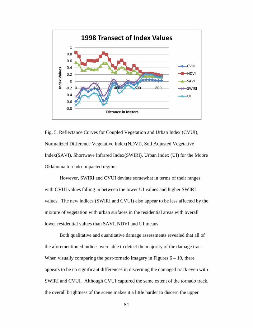
51
Fig. 5. Reflectance Curves for Coupled Vegetation and Urban Index (CVUI),
Normalized Difference Vegetative Index(NDVI), Soil Adjusted Vegetative
Index(SAVI), Shortwave Infrared Index(SWIRI), Urban Index (UI) for the Moore
Oklahoma tornado-impacted region.
However, SWIRI and CVUI deviate somewhat in terms of their ranges
with CVUI values falling in between the lower UI values and higher SWIRI
values. The new indices (SWIRI and CVUI) also appear to be less affected by the
mixture of vegetation with urban surfaces in the residential areas with overall
lower residential values than SAVI, NDVI and UI means.
Both qualitative and quantitative damage assessments revealed that all of
the aforementioned indices were able to detect the majority of the damage tract.
When visually comparing the post-tornado imagery in Figures 6 – 10, there
appears to be no significant differences in discerning the damaged track even with
SWIRI and CVUI. Although CVUI captured the same extent of the tornado track,
the overall brightness of the scene makes it a little harder to discern the upper
-0.8
-0.6
-0.4
-0.2
0
0.2
0.4
0.6
0.8
1
0 200 400 600 800Ind
ex
Val
ue
s
Distance in Meters
1998 Transect of Index Values
CVUI
NDVI
SAVI
SWIRI
UI

52
portion of the damaged path within the residential area. Additionally, all of these
indices had difficulties in capturing portions of the path near the river as well as
the regions of F0/ F1 damages found along the outer edges of the track. However,
the F0/ F1 damages could be discerned quantitatively by comparing reflectance
curves from the same transect in both pre-tornado and post-tornado imagery (see
Figs.4, 5, 11 and 12). These curves illustrate the changes due to the tornado by
curve flattening in some sections and near zero values similar to those of bare soil
or fallow agriculture indicating scattered debris and damaged vegetation.
Fig. 6. 1999 Coupled Vegetation and Urban Image (CVUI) of the Moore,
Oklahoma Tornado-impacted region.

53
Fig. 7. 1999 Urban Index (UI) of the Moore, Oklahoma Tornado-impacted region.
Fig. 8. 1999 Normalized Difference Vegetative Index (NDVI) of the Moore,
Oklahoma Tornado-impacted region.

54
Fig. 9. 1999 Soil Adjusted Vegetative Index (SAVI) for the Moore, Oklahoma
Tornado-impacted region.
Fig. 10. 1999 Shortwave Infrared Vegetative Index (SWIRI) for the Moore,
Oklahoma Tornado-impacted region.
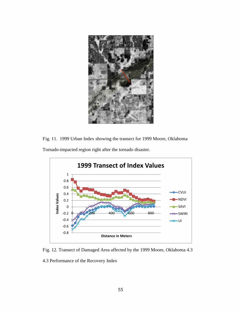
55
Fig. 11. 1999 Urban Index showing the transect for 1999 Moore, Oklahoma
Tornado-impacted region right after the tornado disaster.
Fig. 12. Transect of Damaged Area affected by the 1999 Moore, Oklahoma 4.3
4.3 Performance of the Recovery Index
-0.8
-0.6
-0.4
-0.2
0
0.2
0.4
0.6
0.8
1
0 200 400 600 800Ind
ex
Val
ue
s
Distance in Meters
1999 Transect of Index Values
CVUI
NDVI
SAVI
SWIRI
UI

56
Although the post-tornado images displayed virtually identical damage
patterns, the recovery images highlighted some significant differences between
the indices in terms of the extent of reconstruction. Most notably, both vegetation
indices indicate faster reconstruction than the CVUI, SWIRI and UI recovery
images as seen in Figures 13 – 27. While NDVI and SAVI continue to show
extensive damages similar to CVUI, SWIRI and UI for 2000, the 2001 recovery
images show only minor damages in the residential sections located in the upper
portion of the track and some of the forested regions in the lower left quadrant.
Contrary to the vegetation indices, damage remains more widespread for CVUI,
SWRI and UI scenes in 2001 particularly in the upper right and lower left sections
of the track (Figs. 13-27). Even more contrast between the 2002 recovery
patterns exists with the vegetation indices showing almost complete recovery with
only slight damage to the left of the airport and in the densely vegetative areas of
the lower left quadrant. Contrary to this pattern, the other indices show only
minor recovery changes in 2002 from 2001 with damage still visible in the
residential areas to the left of the airport as well as to the southwest (north of the
river) and in the vegetative areas in the lower left portion of the image.
Unlike the vegetation indices, there were some subtle differences in
reconstruction among the CVUI, SWIRI and UI recovery images. Overall, both
SWIRI and UI displayed nearly identical damage patterns with some discernable
differences with the CVUI recovery scenes (Figs. 13 - 18, 25 - 27). Both SWIRI
and UI showed slightly more damage in some of the residential areas to the north
of the river compared to CVUI in 2000. For the following year, more damage can
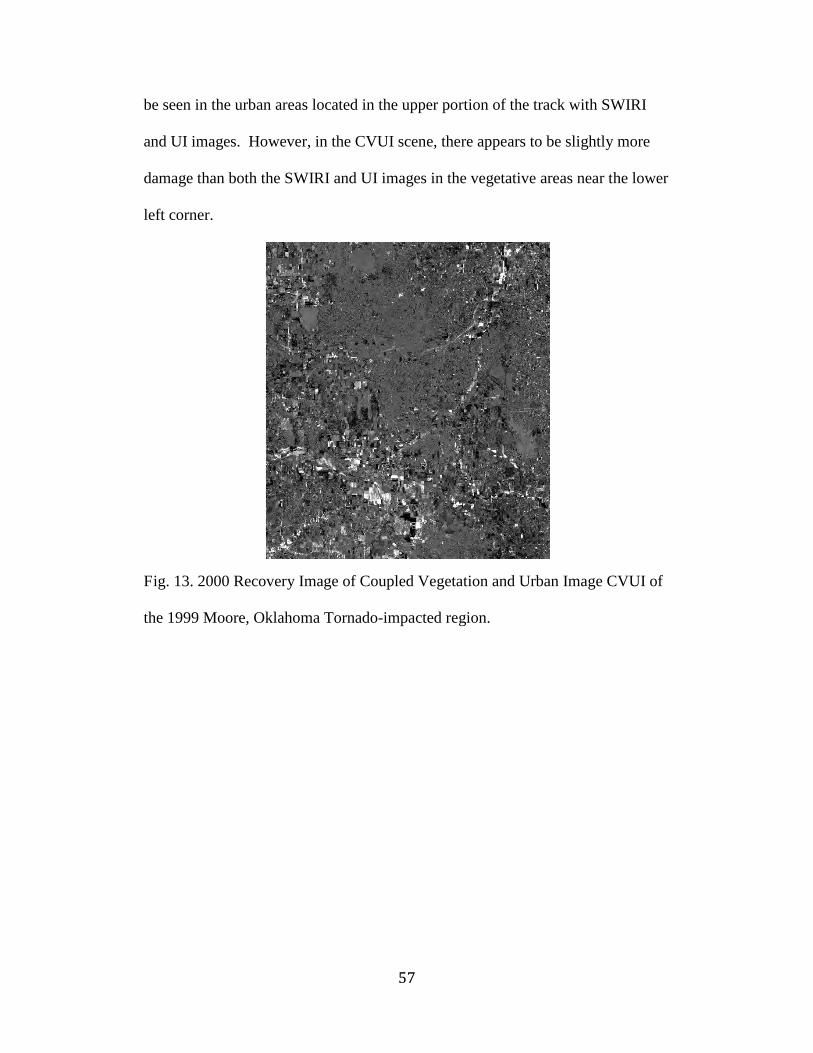
57
be seen in the urban areas located in the upper portion of the track with SWIRI
and UI images. However, in the CVUI scene, there appears to be slightly more
damage than both the SWIRI and UI images in the vegetative areas near the lower
left corner.
Fig. 13. 2000 Recovery Image of Coupled Vegetation and Urban Image CVUI of
the 1999 Moore, Oklahoma Tornado-impacted region.
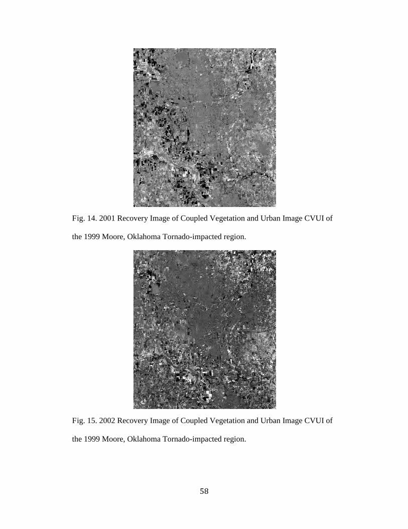
58
Fig. 14. 2001 Recovery Image of Coupled Vegetation and Urban Image CVUI of
the 1999 Moore, Oklahoma Tornado-impacted region.
Fig. 15. 2002 Recovery Image of Coupled Vegetation and Urban Image CVUI of
the 1999 Moore, Oklahoma Tornado-impacted region.
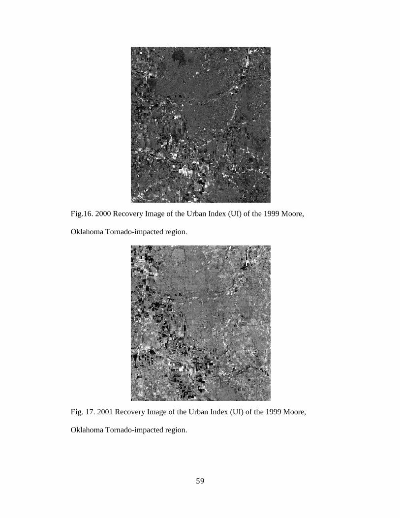
59
Fig.16. 2000 Recovery Image of the Urban Index (UI) of the 1999 Moore,
Oklahoma Tornado-impacted region.
Fig. 17. 2001 Recovery Image of the Urban Index (UI) of the 1999 Moore,
Oklahoma Tornado-impacted region.

60
Fig.18. 2002 Recovery Image of the Urban Index (UI) of the 1999 Moore,
Oklahoma Tornado-impacted region.
Fig. 19. 2000 Recovery Image of Normalized Difference Vegetative Index
(NDVI) of the 1999 Moore, Oklahoma Tornado-region.

61
Fig. 20. 2001 Recovery Image of Normalized Difference Vegetative Index
(NDVI) of the 1999 Moore, Oklahoma Tornado-impacted region.
Fig. 21. 2002 Recovery Image of Normalized Difference Vegetative Index
(NDVI) of the 1999 Moore, Oklahoma Tornado-impacted region.

62
Fig. 22. 2000 Recovery image of Soil Adjusted Vegetative Index (SAVI) of the
1999 Moore, Oklahoma Tornado-impacted region.
Fig . 23. 2001 Recovery image of Soil Adjusted Vegetative Index (SAVI) of the
1999 Moore, Oklahoma Tornado-impacted region.
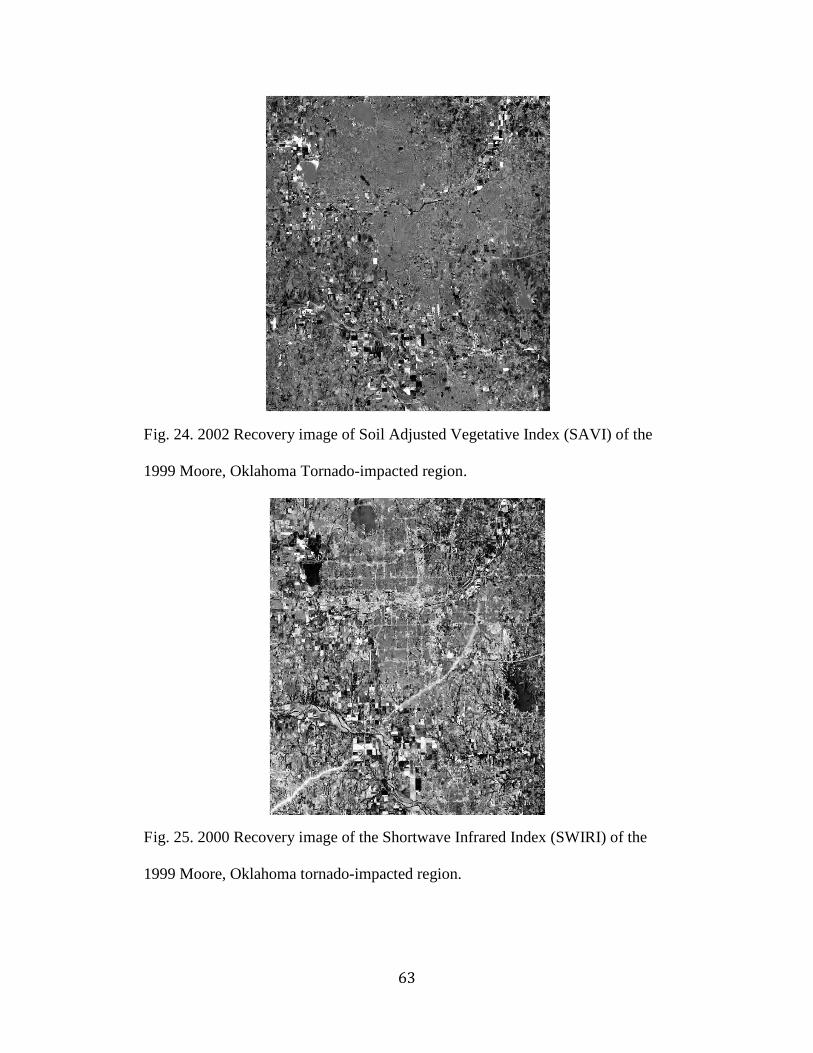
63
Fig. 24. 2002 Recovery image of Soil Adjusted Vegetative Index (SAVI) of the
1999 Moore, Oklahoma Tornado-impacted region.
Fig. 25. 2000 Recovery image of the Shortwave Infrared Index (SWIRI) of the
1999 Moore, Oklahoma tornado-impacted region.
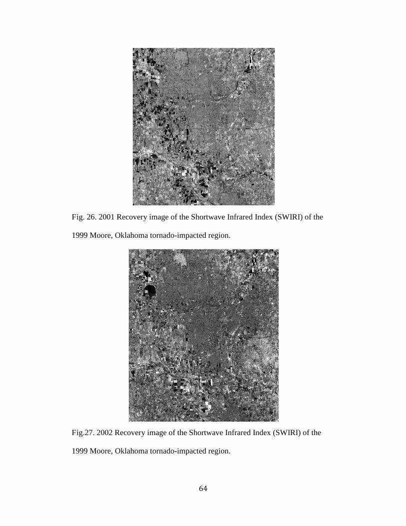
64
Fig. 26. 2001 Recovery image of the Shortwave Infrared Index (SWIRI) of the
1999 Moore, Oklahoma tornado-impacted region.
Fig.27. 2002 Recovery image of the Shortwave Infrared Index (SWIRI) of the
1999 Moore, Oklahoma tornado-impacted region.
65
For 2002, the only minor difference between the CVUI, SWIRI and UI images is
a slightly stronger damage pattern in the urban areas in the upper section of the
track of both SWIRI and UI scenes.
Accuracy assessments of the aforementioned indices and recovery
thresholds revealed several trends. Overall, the 0.5 standard deviation threshold
performed poorly among all the indices with an average overall accuracy of
70.13% based on results listed in Table 4. Within this assessment, the vegetation
indices were found to be the least effective indices with an average overall
accuracy of 66.83% with the lowest overall accuracies of 61.00% and 65.00%
with SAVI for 2000 and 2001 respectively. With only a few exceptions, both the
1.0 and 1.5 standard deviation thresholds were more effective at discerning
reconstruction by an average of 8.0% with overall accuracies above 80.00% for
UI, SWIRI and CVUI. In particular, CVUI and SWIRI yielded the best results
with overall accuracies of 86.00%, 85.00% and 84.00% for CVUI at 1.5 for 2000,
1.0 for 2000 and 1.0 for 2002 followed by 84.00% for both SWIRI 1.5 for 2002
and UI 1.5 for 2000. In addition to the trends of thresholds and spectral
enhancement types, both 2000 and 2002 recovery images generally reported
3.04% higher overall accuracies on average than the 2001 recovery images.
The same trend remained evident with the average overall accuracy
assessments according to the three recovery years by each spectral enhancement
type and threshold combination listed in Table 5. Again, the threshold values of
1.0 and 1.5 standard deviations were more effective at discerning recovery
compared to the 0.5 standard deviation thresholds (Table 5). The latter threshold

66
performed poorly among all the indices with the least effective results of 65.00%
and 68.67% produced by both SAVI and NDVI. Overall, both vegetation indices
underperformed with their best accuracies of 75.67% and 76.33% respectively
still short of the 80% land use/ land change classification (Hord 1976).
Table 4. Accuracy Assessments listed by Index, Standard Deviation Threshold
and Year. (Overall = Overall accuracy, Producer’s. = Producer’s accuracy, User’s
= User’s Accuracy)
Recovery Damaged Overall
Index StDev Year Producer's User's Producer's User's Overall Kappa
NDVI 0.5 2000 61.73% 100.00% 100.00% 38.00% 69.00% 0.3800
NDVI 0.5 2001 63.51% 94.00% 88.46% 46.00% 70.00% 0.4000
NDVI 0.5 2002 65.79% 100.00% 100.00% 48.00% 74.00% 0.4800
NDVI 1 2000 66.22% 98.00% 96.15% 50.00% 74.00% 0.4800
NDVI 1 2001 69.57% 96.00% 93.55% 58.00% 77.00% 0.5400
NDVI 1 2002 71.88% 92.00% 88.89% 64.00% 78.00% 0.5600
NDVI 1.5 2000 71.64% 96.00% 93.94% 62.00% 79.00% 0.5800
NDVI 1.5 2001 73.44% 94.00% 91.67% 66.00% 80.00% 0.6000
NDVI 1.5 2002 75.81% 94.00% 92.11% 70.00% 82.00% 0.6400
SAVI 0.5 2000 56.47% 96.00% 86.67% 26.00% 61.00% 0.2200
SAVI 0.5 2001 74.24% 98.00% 97.06% 66.00% 82.00% 0.6400
SAVI 0.5 2002 77.97% 92.00% 90.24% 74.00% 83.00% 0.6600
SAVI 1 2000 78.33% 94.00% 92.50% 74.00% 84.00% 0.6800
SAVI 1 2001 78.69% 96.00% 94.87% 74.00% 85.00% 0.7000
SAVI 1 2002 84.62% 88.00% 87.50% 84.00% 86.00% 0.7200
SAVI 1.5 2000 60.00% 90.00% 80.00% 40.00% 65.00% 0.3000
SAVI 1.5 2001 64.52% 80.00% 73.68% 56.00% 68.00% 0.3600
SAVI 1.5 2002 63.77% 88.00% 80.65% 50.00% 69.00% 0.3900
SWIRI 0.5 2000 63.01% 92.00% 85.19% 46.00% 69.00% 0.3800
SWIRI 0.5 2001 63.89% 92.00% 85.71% 48.00% 70.00% 0.4000
SWIRI 0.5 2002 65.22% 90.00% 83.87% 52.00% 71.00% 0.4200
SWIRI 1 2000 66.18% 90.00% 84.38% 54.00% 72.00% 0.4400
SWIRI 1 2001 68.33% 82.00% 77.50% 62.00% 72.00% 0.4400
SWIRI 1 2002 66.67% 92.00% 87.10% 54.00% 73.00% 0.4600
SWIRI 1.5 2000 68.12% 94.00% 90.32% 56.00% 75.00% 0.5000
SWIRI 1.5 2001 70.77% 92.00% 88.57% 62.00% 77.00% 0.5400
SWIRI 1.5 2002 75.00% 84.00% 81.82% 72.00% 78.00% 0.5600
UI 0.5 2000 70.15% 94.00% 90.91% 60.00% 79.00% 0.5800
UI 0.5 2001 74.58% 88.00% 85.37% 70.00% 79.00% 0.5800
UI 0.5 2002 74.60% 94.00% 91.89% 68.00% 81.00% 0.6200
UI 1 2000 60.81% 90.00% 80.77% 42.00% 66.00% 0.3200
UI 1 2001 62.32% 86.00% 77.42% 48.00% 67.00% 0.3400

67
Table 4 Con’t
UI 1 2002 69.57% 96.00% 93.55% 58.00% 69.00% 0.3800
UI 1.5 2000 65.71% 92.00% 86.67% 52.00% 72.00% 0.4400
UI 1.5 2001 67.65% 92.00% 87.50% 56.00% 74.00% 0.4800
UI 1.5 2002 67.65% 92.00% 87.50% 56.00% 74.00% 0.4800
CVUI 0.5 2000 62.34% 96.00% 91.30% 42.00% 75.00% 0.5000
CVUI 0.5 2001 69.70% 92.00% 88.24% 60.00% 76.00% 0.5200
CVUI 0.5 2002 70.15% 94.00% 90.91% 60.00% 76.00% 0.5200
CVUI 1 2000 70.77% 92.00% 88.57% 62.00% 77.00% 0.5400
CVUI 1 2001 72.58% 90.00% 86.84% 66.00% 78.00% 0.5600
CVUI 1 2002 74.19% 92.00% 89.47% 68.00% 80.00% 0.6000
CVUI 1.5 2000 77.19% 88.00% 86.05% 74.00% 81.00% 0.6200
CVUI 1.5 2001 78.33% 94.00% 92.50% 74.00% 84.00% 0.6800
CVUI 1.5 2002 76.56% 98.00% 97.22% 70.00% 84.00% 0.6800
Table 5. Averaged Accuracy Assessments listed by Index and Standard Deviation
Threshold. (Overall = Overall accuracy, Prod. = Producer’s accuracy, User’s =
User’s Accuracy, R = Rank, PR = Producer’s Rank, UR= User’s Rank)
Overall Recovery Damaged
IndexSt
Dev Ave. R Prod. User's PR. UR Prod. User's PR. URSAVI 0.5 65.00% 15 62.01% 94.00% 15 4 86.74% 41.33% 14 15SAVI 1.0 75.67% 8 67.32% 93.33% 9 8 89.12% 54.00% 7 10SAVI 1.5 74.33% 9 67.73% 93.33% 8 8 89.05% 55.33% 8 9NDVI 0.5 68.67% 14 62.59% 93.33% 14 8 88.21% 44.00% 11 14NDVI 1.0 76.33% 7 69.49% 94.00% 7 4 90.81% 58.67% 2 7NDVI 1.5 71.00% 12 66.24% 86.00% 12 15 80.00% 56.00% 15 8UI 0.5 73.00% 11 66.42% 93.33% 11 8 89.63% 52.67% 6 12UI 1.0 80.00% 5 74.59% 91.33% 3 12 88.91% 68.67% 9 4UI 1.5 79.00% 6 72.88% 94.00% 6 4 91.44% 64.67% 1 6SWIRI 0.5 73.67% 10 66.85% 94.00% 10 4 90.25% 53.33% 4 11SWIRI 1.0 80.33% 3 74.34% 92.67% 5 10 90.63% 68.00% 3 5SWIRI 1.5 81.67% 1 77.10% 90.00% 2 14 88.19% 73.33% 12 1CVUI 0.5 70.33% 13 64.08% 92.67% 13 10 86.77% 48.00% 13 13CVUI 1.0 80.33% 3 74.53% 92.00% 4 11 89.86% 68.67% 5 3CVUI 1.5 81.67% 1 77.27% 90.67% 1 13 88.74% 72.67% 10 2
UI was consistently better than SAVI and NDVI with the best threshold of one
standard deviation accurately classifying 80% of damaged and recovered pixels
followed by 79.67% for the 1.5 standard deviation threshold. Performing even
better than UI, both new indices, SWIRI and CVUI, were found to be the most
effective indices at capturing yearly reconstruction with the same average overall
68
accuracies of 80.33% and 81.67% for 1.0 and 1.5 standard deviation thresholds
respectively.
Additional accuracy assessments were able to correctly identify recovered
regions in terms of the user’s accuracies, but had some difficulty with the
inclusion of damaged pixels in the recovered class as noted by the producer’s
accuracies. For all the indices, the user’s accuracies were above 86.00%
suggesting little difficulty in classifying recovered pixels. The smallest threshold
of 0.5 standard deviations outperformed the other thresholds with a user’s
accuracy of 94.00% for SAVI, NDVI, SWIRI and UI, while the 1.5 standard
deviation threshold had the greatest difficulty of misclassifying damaged pixels
especially in the case of NDVI. Contrary to the user’s accuracy assessments, the
largest deviations yielded the best results with producer’s accuracies of 77.27%
for CVUI followed by 77.10% for SWIRI. The worst producer’s accuracies
resulted with accuracies below 70.00% from both SAVI and NDVI. Overall, the
producer’s accuracies had more problems excluding recovered pixels from the
damaged class with overall lower results than the user’s accuracies.
Unlike recovered regions, damaged pixels were more difficult to classify
as noted by both lower producer’s and user’s accuracy assessments. While
producer’s accuracies remained at 80.00% or above, these accuracies were still
lower than those of recovered pixels by 19.00% on average. The most effective
results were produced by the UI at 91.44% using 1.5 standard deviation followed
by NDVI and SWIRI at 1.0 standard deviation thresholds with 90.81% and
90.63% respectively. Both 0.5 and 1.5 standard deviation thresholds
69
underperformed with the least effective results of 80.00% reported with NDVI
using the 1.5 standard deviation threshold. Unlike the producer’s accuracies, the
user’s accuracies deviated more with the lowest accuracy of 41.33% noted with
SAVI at 0.5 standard deviation to the highest accuracy of 73.33% reported by
SWIRI at 1.5 standard deviation threshold. Overall, the largest standard deviation
thresholds classified damaged pixels the best using UI, SWIRI and CVUI
compared to the vegetation indices.
Although the larger thresholds reported higher overall accuracies, these
findings were mixed when examining producer’s and user’s accuracies for both
classified damaged and recovered regions. For recovered pixels, the 0.5 standard
deviation threshold had the least problem of including damaged pixels in
recovered class with the highest user’s accuracy of 93.47%, while the 1.5 standard
deviation threshold had the least problems misidentifying recovered pixels as
damaged with the highest producer’s accuracy of 72.24%. For damaged pixels,
the 1.0 standard deviation threshold noted the highest producer’s accuracy of
89.87%, while 1.5 standard deviation threshold reported the highest user’s
accuracy of 64.40%. Overall, the narrower ranges had fewer problems
misidentifying pixels, while the larger ranges were more susceptible to the
inclusion of the wrong class of pixels. However, the larger thresholds could be
less affected by exogenous land use changes such as agricultural practices and
newly built-environments.
4.4 Annual Reconstruction and Recovery Rates

70
Based on the top six overall accuracy assessments, maps depicting
reconstruction over three years portrayed similar recovery trends. These maps
shown in Figures 28 – 33 all suggested complete recovery was never achieved by
2002 with an average of 91.14% recovered in 2002 based on recovery information
listed in Tables 6. In fact, the majority of reconstruction occurred within the first
two years after the disaster by an average of 79.27% with only an 11.87%
increase in 2002. Similar damaged patterns also remained with the vegetative
regions still affected in the lower left quadrant and just south of the river and
residential sections located to the northeast of the river and to the left of the
airport (Figs. 28 - 33).
The type of differences between the recovery maps (Figs. 28 - 33) was
mainly impacted by the threshold selection followed by the spectral enhancement
type (CVUI, NDVI, SAVI, SWIRI, UI). The 1.5 standard deviation threshold
illustrated more reconstruction overall with 94.24% recovered by 2002 compared
to only 88.05% recovered using the 1.0 standard deviation threshold. The
different thresholds also highlighted deviations in annual recovery rates with the
1.5 standard deviation threshold depicting 12.70% more recovery in 2000
compared to the 1.0 standard deviation threshold. Although the latter threshold
portrayed 4.41% more reconstruction in 2001, the former threshold still captured
8.29% more recovery. The former threshold also handled land use changes better
particularly in the case of agricultural fields, which can be seen as distinct linear
shapes in McClain County. These regions were predominantly classified as

71
recovered in 2001 using the former threshold, where as the latter threshold
consistently classified these regions as still damaged even in 2002.
Table 6. Annual Recovery Rates listed by Index, Threshold (Thres.) and Year.
Index Thres. YearRecovered Area
(km)Damaged Area
(km)Total Area
(km)Recovery Rate
(%)
SWIRI 1.5 2000 24,362.10 6,975.90 31,338.00 77.74%
2001 28,655.10 2,682.90 31,338.00 91.44%
2002 29,631.60 1,706.40 31,338.00 94.55%
1.0 2000 20,372.40 10,965.60 31,338.00 65.01%
2001 25,909.20 5,428.80 31,338.00 82.68%
2002 26,928.90 4,409.10 31,338.00 85.93%
CVUI 1.5 2000 24,804.90 6,533.10 31,338.00 79.15%
2001 28,607.40 2,730.60 31,338.00 91.29%
2002 29,391.30 1,946.70 31,338.00 93.79%
1 2000 20,815.20 10,522.80 31,338.00 66.42%
2001 26,239.50 5,098.50 31,338.00 83.73%
2002 27,894.60 3,443.40 31,338.00 89.01%
UI 1.5 2000 24,124.50 7,213.50 31,338.00 76.98%
2001 28,357.20 2,980.80 31,338.00 90.49%
2002 29,575.80 1,762.20 31,338.00 94.38%
1.0 2000 20,161.80 11,176.20 31,338.00 64.34%
2001 25,674.30 5,663.70 31,338.00 81.93%
2002 27,952.20 3,385.80 31,338.00 89.20%
Spectral enhancement types (CVUI, NDVI, SAVI, SWIRI, UI) were also
affected by land cover changes with some noticeable differences determining
recovery in the vegetative regions and urban areas. Focusing on the 1.5 threshold
results, both the CVU and SWIR indices illustrated slightly more damage in the
urban areas located in the upper portion of the track as well as less damage in the
vegetative regions found in the lower portion of the track (Figs. 29 and 31).

72
.
Fig. 28. Map of the 1999 Moore Oklahoma Tornado-impacted region showing
recovered and damaged regions for 2000, 2001 and 2002 using the Coupled
Vegetative and Urban Index (CVUI) and 1.0 standard deviation threshold.

73
Fig. 29. Map of the 1999 Moore Oklahoma Tornado-impacted region showing
recovered and damaged regions for 2000, 2001 and 2002 using the Coupled
Vegetative and Urban Index (CVUI) and 1.5 standard deviation threshold.
Fig. 30. Map of the 1999 Moore Oklahoma Tornado-impacted region showing
recovered and damaged regions for 2000, 2001 and 2002 using the Shortwave
Infrared Index (SWIRI) and 1.0 standard deviation threshold.

74
Fig. 31. Map of the 1999 Moore Oklahoma Tornado-impacted region showing
recovered and damaged regions for 2000, 2001 and 2002 using the Shortwave
Infrared Index (SWIRI) and 1.5 standard deviation threshold.

75
Fig. 32. Map of the 1999 Moore Oklahoma Tornado-impacted region showing
recovered and damaged regions for 2000, 2001 and 2002 using the Urban Index
(UI) and 1.0 standard deviation threshold.
Fig. 33. Map of the 1999 Moore Oklahoma Tornado-impacted region showing
recovered and damaged regions for 2000, 2001 and 2002 using the Urban Index
(UI) and 1.5 standard deviation threshold.
Although CVUI and SWIRI displayed nearly identical damage patterns,
more damage can be seen in urban areas in the top of the track in the case of
CVUI (Fig. 29). CVUI, in particular, had the least problem in misclassifying
agricultural changes as damaged areas when comparing the bottom portion of the
track to the other indices, whereas, UI proved to be the most problematic with
more fields misidentified as damaged in the middle and bottom portions of the
track. Other differences among the indices could be seen in annual recovery rates
76
with the CVUI, SWIR and UI reporting the largest reconstruction for 2000, 2001
and 2002 respectively (Figs. 27, 29 and 31).
4.5 Recovery Rates as a Function of the Fujita Scale
By establishing recovery through the investigation of different indices and
thresholds in the previous analysis, recovery rates were determined to examine
whether or not the level of damage played a key role in reconstruction. The first
major finding of this analysis for the top six recovery indices and thresholds is the
consistent theme that the incredibly damaged regions associated with an F-5
rating were the slowest to recover, while the F0/F1 regions comprised of minor
damages reported the highest recovery rates. Specifically, in the first year
following the tornado event (2000), recovery from F0/F1-F3 damage occurred by
an average 73.45%, while the most substantial damage of F4-F5 only recovered
by an average of 58.69%. Even by the third year after the tornado event (2002),
recovery for the F5 zone was only 75.32% while F0/F1 damage had recovered to
94.07%.
Individual differences in recovery rates based on F-scale zones were
affected by threshold selection and spectral enhancement type as a result of the
previous analysis. The main differences were attributed to threshold selection
with the 1.5 standard deviation reporting 12.88%, 8.14% and 6.34% more
recovery on average for all the indices than the 1.0 standard deviation for 2000,
2001 and 2002 respectively (Table 6). The most significant differences occurred
during the first year after the tornado disaster with these deviations tapering off in
2001 and even more so in 2002. However, the SWIR index with the 1.5 standard

77
deviation threshold reported anomalously higher values in 2002 that varied from
6.54% to 10.58% with the largest rate increase in the F4 zones. As a result, the
SWIR index at the 1.5 standard deviation threshold had the highest recovery rates
for 2002 with the exception of UI reporting the highest recovery rate for the F5
zone for both thresholds. Despite this result, the CVU index displayed the highest
recovery rates overall for both thresholds followed by the SWIR index with the
lowest recovery rates reported by UI.
Using the information from the top six recovery results (Table 6), recovery
rates for each F-scale zone were averaged for further analysis according to each
year after the event. For any particular year (2000-2002), those values (Table 7)
illustrated that recovery in the F5 damage zones consistently lagged behind the
F0/F1 zone throughout 2000, 2001, and 2002 by a noticeable difference of
22.21%, 17.13% and 18.76% respectively. The recovery rates for the F4 zones
were also distinctly lower than the F0/F1 – F3 recovery rates with these lesser-
damaged regions exhibiting very similar behavior in terms of slope and range.
When the averaged values were plotted by year (Fig. 34), a significant
difference in recovery rates was evident between 2000 and 2001 as opposed to
2001 to 2002 for all damaged levels. The 2000-2001 rates displayed a 12.59% -
18.15% increase in recovery, while the 2001-2002 recovery rates increased from
2.05% to 5.55%. Other deviations regarding slope could be seen from 2001 to
2002 as the F4 zone reported the highest change in recovery by 5.55%, while the
F5 recovery rate nearly plateaued with only a 2.05% increase in 2002 with a total

78
75.32% recovered. Conversely, F0/F1-F3 recovery rates from 2000 to 2002
produced nearly identical slopes and a relatively narrow range.
Table 7. Recovery Rates for F-scale zones listed by Index, Threshold (Thres.) and
Year.
Index Thres. YearF-scaleZone
RecoveredArea (km)
Damaged Area(km)
Total Area(km)
RecoveryRate(%)
SWIR 1.5 2000 1 8,149.50 1,701.00 9850.5 82.73%2 6,468.30 1,744.20 8,212.50 78.76%3 6,130.80 1,881.00 8,011.80 76.52%4 3,174.30 1,400.40 4,574.70 69.39%5 439.20 249.30 688.50 63.79%
2001 1 9,293.40 557.10 9850.5 94.34%2 7,591.50 621.00 8,212.50 92.44%3 7,322.40 689.40 8,011.80 91.40%4 3,916.80 657.90 4,574.70 85.62%5 531.00 157.50 688.50 77.12%
2002 1 9,544.50 306.00 9850.5 96.89%2 7,842.60 369.90 8,212.50 95.50%3 7,596.00 415.80 8,011.80 94.81%4 4,110.30 464.40 4,574.70 89.85%5 538.20 150.30 688.50 78.17%
CVUI 1.5 2000 1 8,298.90 1,551.60 9,850.50 84.25%2 6,583.50 1,629.00 8,212.50 80.16%3 6,236.10 1,775.70 8,011.80 77.84%4 3,231.90 1,342.80 4,574.70 70.65%5 454.50 234.00 688.50 66.01%
2001 1 9,290.70 559.80 9,850.50 94.32%2 7,598.70 613.80 8,212.50 92.53%3 7,304.40 707.40 8,011.80 91.17%4 3,884.40 690.30 4,574.70 84.91%5 529.20 159.30 688.50 76.86%
2002 1 9,502.20 348.30 9,850.50 96.46%2 7,786.80 425.70 8,212.50 94.82%3 7,512.30 499.50 8,011.80 93.77%4 4,051.80 522.90 4,574.70 88.57%5 538.20 150.30 688.50 78.17%
SWIR 1.0 2000 1 6,997.50 2,853.00 9,850.50 71.04%2 5,411.70 2,800.80 8,212.50 65.90%3 5,060.70 2,951.10 8,011.80 63.17%4 2,555.10 2,019.60 4,574.70 55.85%5 347.40 341.10 688.50 50.46%
2001 1 8,494.20 1,356.30 9,850.50 86.23%2 6,874.20 1,338.30 8,212.50 83.70%3 6,583.50 1,428.30 8,011.80 82.17%4 3,471.30 1,103.40 4,574.70 75.88%5 486.00 202.50 688.50 70.59%
2002 1 8,831.70 1,018.80 9,850.50 89.66%2 7,126.20 1,086.30 8,212.50 86.77%3 6,851.70 1,160.10 8,011.80 85.52%4 3,626.10 948.60 4,574.70 79.26%

79
Table 7 Con’t5 493.20 195.30 688.50 71.63%
CVUI 1.0 2000 1 7,203.60 2,646.90 9,850.50 73.13%2 5,516.10 2,696.40 8,212.50 67.17%3 5,129.10 2,882.70 8,011.80 64.02%4 2,597.40 1,977.30 4,574.70 56.78%5 369.00 319.50 688.50 53.59%
2001 1 8,631.00 1,219.50 9,850.50 87.62%2 7,022.70 1,189.80 8,212.50 85.51%3 6,612.30 1,399.50 8,011.80 82.53%4 3,484.80 1,089.90 4,574.70 76.18%5 488.70 199.80 688.50 70.98%
2002 1 9,081.00 769.50 9,850.50 92.19%2 7,411.50 801.00 8,212.50 90.25%3 7,118.10 893.70 8,011.80 88.85%4 3,784.50 790.20 4,574.70 82.73%5 499.50 189.00 688.50 72.55%
UI 1.5 2000 1 8,220.60 1,629.90 9,850.50 83.45%2 6,488.10 1,724.40 8,212.50 79.00%3 5,998.50 2,013.30 8,011.80 74.87%4 3,031.20 1,543.50 4,574.70 66.26%5 386.10 302.40 688.50 56.08%
2001 1 9,228.60 621.90 9,850.50 93.69%2 7,527.60 684.90 8,212.50 91.66%3 7,261.20 750.60 8,011.80 90.63%4 3,817.80 756.90 4,574.70 83.45%5 522.00 166.50 688.50 75.82%
2002 1 9,543.60 306.90 9,850.50 96.88%2 7,827.30 385.20 8,212.50 95.31%3 7,568.10 443.70 8,011.80 94.46%4 4,095.00 479.70 4,574.70 89.51%5 541.80 146.70 688.50 78.69%
UI 1 2000 1 7,115.40 2,735.10 9,850.50 72.23%2 5,438.70 2,773.80 8,212.50 66.22%3 4,941.00 3,070.80 8,011.80 61.67%4 2,366.10 2,208.60 4,574.70 51.72%5 300.60 387.90 688.50 43.66%
2001 1 8,490.60 1,359.90 9,850.50 86.19%2 6,830.10 1,382.40 8,212.50 83.17%3 6,522.30 1,489.50 8,011.80 81.41%4 3,361.50 1,213.20 4,574.70 73.48%5 469.80 218.70 688.50 68.24%
2002 1 9,098.10 752.40 9,850.50 92.36%2 7,426.80 785.70 8,212.50 90.43%3 7,134.30 877.50 8,011.80 89.05%4 3,792.60 782.10 4,574.70 82.90%5 500.40 188.10 688.50 72.68%
Table 8. Recovery Rates for F-scale zones listed by Index, Threshold and Year.
F-scale Zone
Percent (%)Recovered
in 2000
Percent (%)Recovered
in 2001
Percent (%)Recovered
in 2002
1 77.81% 90.40% 94.07%
2 72.87% 88.17% 92.18%

80
Table 8 Con’t3 69.68% 86.55% 91.08%
4 61.77% 79.92% 85.47%
5 55.60% 73.27% 75.32%
When the averaged recovery values were plotted by F-scale damage (Fig.
35), the most recovery at all levels occurred within the first two years after the
event with relatively minor changes between 2001 and 2002. Interestingly, the
recovery lines were not parallel across all damage levels, indicating that there
were differences in the degree of recovery as a function of F-scale damage. The
biggest slope was associated with the 2000 recovery line and the smallest slope
was displayed by the 2002 recovery line. In particular, in 2002, the plotted values
of recovery between F1, F2, F3 and F4 were similar in terms of creating a nearly
horizontal line while the F5 values are still substantially lower.
Fig. 34. Graph for the 1999 Moore Oklahoma Tornado-impacted region
displaying annual recovery rates for 2000, 2001 and 2002 in percent by F-scale
intensity as established by the recovery index.
50.00%55.00%60.00%65.00%70.00%75.00%80.00%85.00%90.00%95.00%
100.00%
1 2 3 4 5
Re
cove
ryin
Pe
rce
nt
(%)
F-scale rating
Annual Recovery by F-scale rating
2000
2001
2002
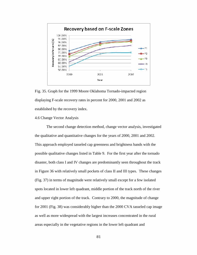
Fig. 35. Graph for the 1999 Moore Oklahoma Tornado
displaying F-scale recovery rates in percent for 2000, 2001 and 2002 as
established by the recove
4.6 Change Vector Analysis
The second change detection method, change vector analysis, investigated
the qualitative and quantitative changes for t
This approach employed tasseled cap greenness and brightness band
possible qualitative changes listed in Table
disaster, both class I and IV changes are predominantly seen throughout the track
in Figure 36 with relatively small pockets of class II and III types. These
(Fig. 37) in terms of magnitude were relatively small except for a few isolated
spots located in lower left quadrant, middle portion of the track north of the river
and upper right portion of the track.
for 2001 (Fig. 38) was considerably higher than the 2000 CVA tasseled cap image
as well as more widespread with the largest increases concentrated in the rural
areas especially in the vegetative regions in the lower left quadrant and
81
Graph for the 1999 Moore Oklahoma Tornado-impacted region
scale recovery rates in percent for 2000, 2001 and 2002 as
established by the recovery index.
4.6 Change Vector Analysis
The second change detection method, change vector analysis, investigated
the qualitative and quantitative changes for the years of 2000, 2001 and 2002
approach employed tasseled cap greenness and brightness bands with the
possible qualitative changes listed in Table 9. For the first year after the tornado
disaster, both class I and IV changes are predominantly seen throughout the track
with relatively small pockets of class II and III types. These
) in terms of magnitude were relatively small except for a few isolated
spots located in lower left quadrant, middle portion of the track north of the river
and upper right portion of the track. Contrary to 2000, the magnitude of change
) was considerably higher than the 2000 CVA tasseled cap image
as well as more widespread with the largest increases concentrated in the rural
areas especially in the vegetative regions in the lower left quadrant and
The second change detection method, change vector analysis, investigated
he years of 2000, 2001 and 2002.
s with the
. For the first year after the tornado
disaster, both class I and IV changes are predominantly seen throughout the track
with relatively small pockets of class II and III types. These changes
) in terms of magnitude were relatively small except for a few isolated
spots located in lower left quadrant, middle portion of the track north of the river
of change
) was considerably higher than the 2000 CVA tasseled cap image
as well as more widespread with the largest increases concentrated in the rural

82
agricultural areas south of the river. As a result, type IV class changes were
observed for every pixel throughout the track, therefore a map was not produced.
The 2002 change vector image had very similar changes in terms of magnitude
(Figure 39), but observed type II class changes instead of type IV in the entire
track.
Table 9. List of land class types and associated land use changes
Class Type of Change
I Increase in Greenness, Increase in Brightness
II Increase in Brightness, Decrease in Greenness
III Decrease in Greenness, Decrease in Brightness
IV Decrease in Brightness, Increase in Greenness
Fig. 36. Change Vector Analysis Map of the 1999 Moore Oklahoma Tornado-
impacted region for 2000 showing different land class changes.

83
Fig. 37. Map of the 1999 Moore Oklahoma Tornado-impacted region showing the
magnitude of changes for 2000 using change vector analysis.
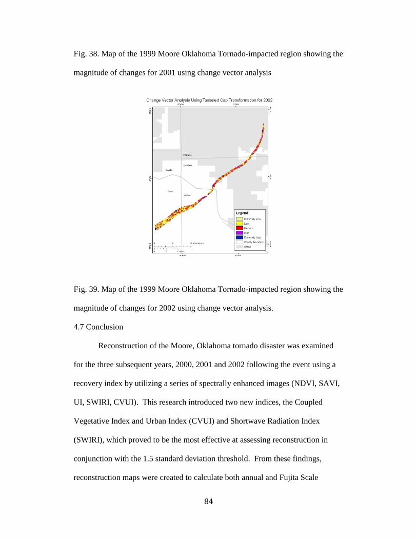
84
Fig. 38. Map of the 1999 Moore Oklahoma Tornado-impacted region showing the
magnitude of changes for 2001 using change vector analysis
Fig. 39. Map of the 1999 Moore Oklahoma Tornado-impacted region showing the
magnitude of changes for 2002 using change vector analysis.
4.7 Conclusion
Reconstruction of the Moore, Oklahoma tornado disaster was examined
for the three subsequent years, 2000, 2001 and 2002 following the event using a
recovery index by utilizing a series of spectrally enhanced images (NDVI, SAVI,
UI, SWIRI, CVUI). This research introduced two new indices, the Coupled
Vegetative Index and Urban Index (CVUI) and Shortwave Radiation Index
(SWIRI), which proved to be the most effective at assessing reconstruction in
conjunction with the 1.5 standard deviation threshold. From these findings,
reconstruction maps were created to calculate both annual and Fujita Scale
85
recovery rates. Annual recovery rates illustrated that complete recovery was
never achieved with the majority of reconstruction occurred within the first two
years. While these findings held true across all of the F-scale recovery rates, the
critical finding in this analysis is that recovery was a direct and significant
function of the level of damage sustain, as measured by the Fujita Scale. The
most damaged area assessed with an F5 rating consistently lagged in recovery
behind the lesser-damaged zones of F0/F1-F3 ratings with the explanation of
these findings discussed in the next chapter.

86
5. Discussion
5.1 Introduction
This research examined the recovery of the Moore, Oklahoma tornado
utilizing remote sensing techniques with medium resolution satellite imagery to
assess whether or not the level of damage sustained impacted recovery rates as
measured by the Fujita Scale. The degree of restoration and recovery was
determined by employing a recovery index with different thresholds on a series of
transformed images (NDVI, SAVI, UI, SWIRI, CVUI). The findings from this
research can be segregated into two broad categories, the results involving the
assessment of the recovery index and its effectiveness and the results involving
the use of that index in the interpretation of tornado recovery.
With regard to the remote sensing aspect, the first major finding was that
medium resolution satellite imagery such as Landsat TM and ETM+ can be used
to establish both annual and F-scale recovery rates. Secondly, the two new
indices, the Shortwave Infrared Index (SWIRI) and the Coupled Vegetation and
Urban Index (CVUI), developed for disaster management and reconstruction
proved to be best suited for assessing recovery over the Urban Index (UI),
Normalized Difference Vegetation Index (NDVI) and Soil Adjusted Vegetation
Index (SAVI). In addition to transformation types, recovery was most effectively
captured using the 1.5 standard deviation threshold with the best overall results
noted with SWIRI at the same threshold.
With regard to tornado recovery interpretation using these top-performing
results, analysis of both annual recovery rates and F-scale recovery rates revealed

87
two significant findings. The first and most critical finding in this part of my
analysis was that the level of damage sustained was a direct and significant
function of recovery. The second important finding in this section was that
complete recovery was never achieved by 2002 even within the F-scale zones.
This chapter discusses the findings of these results.
5.2 Remotely Sensed Data and Recovery Index
Overall, reconstruction of the 1999 Moore, Oklahoma tornado could be
discerned using geospatial techniques with medium resolution imagery of Landsat
Thematic Mapper and Landsat Enhanced Thematic Mapper (30 meters per pixel).
The medium resolution imagery was able to capture the chaotic nature the tornado
track effectively by detecting the deviations within regular patterns of spatially
arranged ground features such as residential neighborhoods and other urban areas.
Using the same premise, reconstruction was then assessed based on changes in the
damage pattern on an annual basis for the specific years of 2000, 2001 and 2002.
Although detailed damages to individual buildings, roads or trees and
reconstruction were not discernable, Landsat imagery considered the recovery of
ground features together with the bigger pixel size. Therefore, this imagery
provided a top view assessment that could have otherwise been missed with the
finer resolution data such as QuickBird or Ikonos imagery.
The degree to which recovery could be accurately discerned proved to be a
function of threshold selection and spectral enhancement type. In regards to
threshold, average overall accuracy assessments revealed that the 1.0 standard
deviation threshold better represented recovery by 78.53% compared to 77.53%

88
with the 1.5 standard deviation threshold. However, both of these thresholds
outperformed the 0.5 standard deviation threshold by an average of 8.00%. This
finding suggested that the larger range of values were more reflective of the actual
reconstruction similar to previous studies (Roemer et al. 2011, Lin et al. 2004)
that also employed thresholds to define damaged and recovered pixels in
subsequent recovery year. By employing a threshold with the recovery index,
exogenous deviations were minimized due to climate deviations in index values
or land use changes, thus reducing the possibility of misclassifying recovered
regions as still damaged.
The use of a recovery threshold does pose some limitations in terms of
accurately classifying damaged and recovered regions due to range of values
representing recovery. Generally, the narrow range of recovered values
associated the smaller thresholds had fewer problems misidentifying recovered
pixels. However, this threshold had more difficulty accurately classifying
damaged pixels. Conversely, the wider range of recovered pixels made the larger
thresholds more susceptible to the inclusion of damaged pixels in the recovered
class. Despite this limitation, the larger thresholds were more effective at
classifying damaged pixels and were able to best capture the recovery process
similar to the findings of Roemer et al. 2011 and Lin et al. 2004.
Regardless of threshold selection, damaged pixels proved to be the most
difficult to accurately classify due to different land use and land cover changes.
In particular, changes in agricultural practices such as fallow versus active field
were repeatedly misidentified as damaged when performing classification
89
accuracy assessments. Additionally, newly constructed urban surfaces were more
likely to be misclassified as damaged especially if this transformation occurred in
previously healthy vegetation areas. Such a change occurred with the
construction of the H.E. Bailey Turnpike Norma Spur (OK 4) in the lower left
quadrant of all 2000 recovery images (Figs 13, 16, 19, 22, and 25) and 2000
tasseled cap magnitude image (Figs. 36 and 37). This land use change was
repeatedly misidentified as damaged among all the thresholds during the
classification accuracy assessments and may have affected the surrounding
vegetation creating false damage areas. Consequently, these exogenous changes
did affect the overall accuracy of the recovery index, but were rather minimal in
comparison to the amount of reconstruction that was accurately identified.
In addition to threshold selection, spectral enhancement type also played a
significant role in the performance of the recovery index. The vegetation indices,
Normalized Difference Vegetation Index (NDVI) and Soil Adjusted Vegetation
Index (SAVI), were the least effective in capturing the recovery process with an
average overall accuracy assessment of 66.83%. Although these indices have
been extensively employed in disaster studies, damaged and non-damaged areas
have been confused in the urban environment due to relatively narrow range of
values (Yuan et al. 2002, Jedlovec et al. 2006). Such signature confusion could
have hindered correctly identifying recovered pixels during the recovery
assessment. Additionally, SAVI and NDVI values can also fall prey to sun
illumination effect even with radiometric corrections and normalization. Such
differences between years could result in erroneous classification of damaged or

90
recovered pixels (McDonald et al. 1998, Lu et al. 2004). The composition of
vegetation could also affect the ability to discern recovery, as SAVI is generally
more suited for densely vegetative areas (Villa 2007). This finding may explain
why SAVI consistently reported the lowest accuracies given that prairie grasses
and agricultural fields generally dominate this study area with relatively small
areas of densely forested regions.
Contrary to the vegetation indices, the Shortwave Infrared Index (SWIRI),
the Coupled Vegetation and Urban Index (CVUI) and the Urban Index (UI) were
more effective at discerning the recovery process. This finding could be
explained, in part, by the use of the mid-infrared bands in conjunction with the
near-infrared band with all these indices. The mid-infrared bands (bands 5 and 7)
can differentiate between different geology types and urban surfaces, while the
near-infrared band measures vegetation health (Lillesand et al. 2004, Sabins 1997,
Bentley et al. 2002). As a result, these indices have a wider range of values for
non-vegetative surfaces and therefore, could better discriminate between damaged
and recovered regions especially in the urban areas. Additionally, the contrast
between the tornado track and surrounding areas also made it easier to discern
damaged from recovered pixels in the tornado track for each recovery year,
thereby improving classification accuracy results.
Among these indices, SWIRI at the 1.5 standard deviation threshold
yielded the best results followed by CVUI using the same threshold. Unlike CVUI
or UI, SWIRI uses the first mid-infrared band (band 5). This is critical because in
addition to discriminating between geology types and urban surface, this band
91
also measures moisture content in soil and vegetation. Therefore, the use of this
band could further discriminate vegetative health as well as discern reconstruction
in the built-environment. This may explain why SWIRI outperformed CVUI and
UI even though UI and SWIRI had nearly identical damage and reconstruction
patterns. Although SWIRI yielded the best results, CVUI better handled
vegetative recovery of agricultural fields and densely vegetative areas. This
finding could be attributed to a better assessment of vegetation restoration with
the NDVI component, as this index is a product of NDVI and UI.
Other factors that could have affected the accuracy of the recovery index
were the quality of the images and sampling points for accuracy assessments. For
example, cloud-free imagery could not be obtained within the desired two weeks
of the anniversary date due to normal springtime storm activity for this region.
As a result, atmospheric conditions between images may be different despite
radiometric correction attempts to obtain apparent reflectance values for ground
features. In addition to atmospheric effects, climate conditions were also
significantly different at the acquisition time for 1999, 2000, 2001 and 2002. The
first year after the tornado (2000) was an abnormally wet year and then the
subsequent years were abnormally dry for April 2001 and September 2002 (OCS
2010b). Although normalization procedures should minimize variations between
scenes, some differences could still exist especially in the vegetative areas.
In addition to climate and atmospheric differences, other problems from
pixel misregistration and distribution of sampling points could have affected
classification accuracies. Locational errors may still exist between scenes despite

92
co-registration efforts, as complete pixel misregistration is unattainable. While
the same approach of stratified random sampling was used, these points were
randomly generated and not reused for each accuracy assessment. The location of
these points could have a big impact on the accuracy assessment especially if
there was a rather high concentration of points in erroneous classified damaged
areas such as agricultural fields or on the newly constructed H.E. Bailey Turnpike
Norman Spur.
Despite some of these problems, the recovery index was able to correctly
identify reconstruction with SWIRI and CVUI using the 1.5 and 1.0 standard
deviation thresholds with overall accuracies of 81.67% and 80.33% respectively.
The next best results were reported with UI using the larger thresholds with
overall accuracies of 80% and 79.33%. Among the best indices, damage patterns
were fairly consistent in showing damage in the densely vegetative areas in the
lower quadrant and in the urban areas just south of the river and upper portion of
track. These regions were some of the hardest hit areas sustaining F4 and F5
damages and would reasonably take longer to recover.
5.3 Recovery Rates as a Function of F-scale
From these top-performing results, I analyzed recovery rates for three
years following the 1999 Moore, Oklahoma tornado and established two
significant findings. The first and most critical finding in this analysis revealed
that the incredibly damaged areas associated with an F-5 rating were the slowest
to rebuild, while the lesser-damaged areas of F0/F1 ratings reported the highest
recovery rates. These results were consistent throughout 2000, 2001 and 2002 as

93
reconstruction in F5 damaged areas lagged behind F0/F1 damaged zones by a
considerable difference of 22.21%, 17.13%, and 18.76% respectively. The
recovery rates for F4 damaged areas were also significantly lower than the F0/F1
– F3 recovery rates for all the recovery years illustrating that the scope and
magnitude of the disaster has a profound and direct effect on recovery. This
finding is conclusive with other hazard studies (Dacy and Kuerether 1969, Haas et
al. 1977, Yasui 2007, Aldridge 2011) that have also found recovery rates to be a
function of the biophysical impact.
Higher reconstruction in the F0/F1-F3 damaged areas could be explained
by the contrasting differences in associated damages between these regions and
those associated with F4 and F5 ratings. Maximum damage indicators for F0/F1-
F3 ratings are noted by missing roofs and in some cases removal of walls, while
in F-4 rated damaged zones, well-constructed houses are leveled and weaker
structures are carried away for some distance (Fujita 1971). Damages associated
with F5 ratings are the most severe, as well-constructed structures are leveled and
carried away, trees debarked and automobile-sized missiles are generated (Fujita
1971). As a result, reconstruction within the lesser-damaged areas (F0/F1 – F3)
would typically require less financial resources to draw upon and time in
completing the repairs (Dacy and Kunreuther 1969, Yasui 2007, Finch et al. 2010,
Aldridge 2011). This would explain the similar reconstruction rates and faster
recovery in the F0/F1 – F3 damaged zones. Unlike the lesser-damaged areas,
reconstruction in the most severely damaged areas (F4 and F5) would likely
require more financial resources and time rebuild. Severely damaged buildings
94
and other infrastructure would also likely involve decision-making policies
regarding construction type, permits and even possibly relocation, therefore
requiring more time to complete (Finch et al. 2010).
In addition to anthropogenic reconstruction, vegetation regeneration is a
function of the magnitude of damage and plant size. Generally minor-wind
damages to vegetation will re-orient or blow over the plant, resulting in only
minor disruptions in photosynthetic activity (Bentley et al. 2002). Therefore,
much of the vegetation survives and recovers quickly back to the pre-tornado
state. Contrary to this, intense winds are more likely to snap the vegetation and
consequently destroy it recovering much slower. Additionally, the speed to which
vegetation regenerates also depends on plant size before the disaster, as smaller
plants such as short grasses or small shrubs tend to recover quicker than large
trees (Peterson 2000). Typically, larger vegetation will take several years if not
decades for complete restoration based on tree size (Peterson 2000). This aspect
explains not only the vegetative response in terms of recovery rates, but also the
location of still damaged areas in the bottom portion of the track due to the
densely forested region.
Annual recovery, utilizing the F-scale assessment of tornado damages,
also revealed that most reconstruction occurred within the first two years. During
the first year, the average recovery rate for all F-scale damage zones was 67.55%
indicating rather rapid reconstruction over the assessed time period. Typically,
after such a disaster, high priority is placed on reestablishing infrastructure and
rebuilding structures with minor damages in attempt to return to pre-disaster

95
conditions (Uitto 1998, Mitchell 1999). Other structures may take longer to
rebuild due to available financial resources, amount of disaster relief, and
decision-making policies (Finch et al. 2010). This would explain the additional
12.59% - 18.15% increase in recovery from 2000 to 2001. However, for 2001 –
2002, reconstruction only improved by 2.05% to 5.55% indicating that most
recovery occurred within the first two years. Recovery probably tapered off due
to the timing of insurance settlements and disaster relief payments within the first
couple of years, as most rebuilding occurs soon after the distribution of funds.
Additionally, temporary housing could also turn into permanent residence as
society becomes more settled with time, therefore foregoing complete
reconstruction in certain areas.
Within this recovery assessment, the second important finding was that
even by 2002, three years after the tornado event, complete recovery was never
achieved within any of the F-scale damaged zones. By 2002, the least damaged
regions (F0/F1) had rebuilt to 94.07%, while reconstruction in the most incredibly
damaged areas (F5) had reached only 75.32%. Part of this reason could be
accredited with too short assessment period, given that a subsequent F4 tornado
hit the same study area on May 8, 2003, thereby missing any continued
reconstruction. Different land use and land changes also could occur during the
recovery process as a result of decision-making policies and political institutions
seeking to either mitigate future events or help improve current economic status.
Additionally, individual decisions to relocate could also impact reconstruction
based on damage severity, financial resources, and psychological decisions to

96
rebuild in the same area. With regards to vegetation regeneration, large-scale
vegetation in terms of trees and large shrubs will take several years if not decades
to return to pre-tornado conditions, thus contributing to incomplete recovery.
In addition to the biophysical aspect of disaster, pre-existing conditions
could also affect recovery in terms of social vulnerabilities and place-based
vulnerabilities. Social vulnerabilities consider the pre-existing social conditions
of age, race, ethnicity, dwelling type, socioeconomic status, political institutions
and other social variables in conjunction with the biophysical impact of the
disaster (Liverman 1990, Blaikie et al 1994, Cutter 1996, Cutter 2000, Cutter et
al. 2003). Lower socioeconomic status, lack of resources and poor housing
quality can magnify the impact of the disaster and consequently affect the ability
to fully recover (Liverman 1990, Blaikie et al 1994, Cutter 1996, Cutter et al.
2003). Such examples of this can be seen in the more recent cases of 2004
Tsunami, Hurricane Katrina, the Haitian Earthquake (Kaplan et. al 2009, Cutter et
al. 2006). These factors could have contributed to the incomplete reconstruction
after the tornado disaster, but were not analyzed in this analysis. Future research
would need to examine these social vulnerabilities in conjunction with the
biophysical impact for a complete recovery assessment.
Certain geographic locations may also be physically and socially
susceptible to a given hazard creating place-based vulnerabilities (Liverman 1990,
Cutter 1996). These regions can have higher degrees of vulnerability based on the
clustering of social and biophysical characteristics within the hazard zone (Cutter
et al. 2000). The city of Moore, Oklahoma was previously struck by a tornado in

97
October 1998, but that tornado produced considerably smaller damages with a
maximum F-scale rating of F2 and path length of only 2 miles. Nonetheless, this
could have affected individual and commercial decisions with regard to rebuilding
or re-locating. One known example occurred in a residential section of Moore,
Oklahoma as decision-makers chose not to rebuild in this section due to the past
occurrence of tornadoes in this area and instead dedicated the land as a city park.
Other place-based vulnerabilities, similar to the aforementioned, could have also
existed within the track and affected individual and policy-making decisions on
reconstruction given the short time between disasters.
5.4 Conclusion
This research examined the reconstruction of the 1999 Moore, Oklahoma
tornado for the years of 2000, 2001, and 2002 utilizing remote sensing imagery
and change detection methods. The use of medium resolution imagery provided
to top-view assessment of reconstruction in which recovery was determined
employing a recovery index and different thresholds on a series of spectrally
enhanced images (NDVI, SAVI, UI, SWIRI, CVUI). With these spectrally
enhanced images, the two new indices, the Shortwave Infrared Index (SWIRI)
and the Coupled Vegetation and Urban Index (CVUI), developed for disaster
management and reconstruction proved to be best suited for assessing recovery
over the Urban Index (UI), Normalized Difference Vegetation Index (NDVI) and
Soil Adjusted Vegetation Index (SAVI). In addition to transformation types,
recovery was most effectively captured using the 1.5 standard deviation threshold
with the best overall results noted with SWIRI at the same threshold. This

98
threshold accounted for annual deviations between scenes in terms of climate and
atmospheric condition and non-damaged land use changes mainly in agricultural
areas.
From these top-performing results, I analyzed the recovery rates and
established two significant findings. The most critical finding in this research
discovered that most severely damaged areas associated with an F5 rating were
the slowest to recover, while the lesser damaged areas associated with F0/F1
ratings were the quickest to recover. These results were consistent throughout
2000, 2001 and 2002 as reconstruction for F5 zones consistently lagged the F0/F1
zones by 22.15%, 17.13%, and 18.76% respectively. Recovery rates for F4
damaged areas were also significantly lower than those of the lesser damaged
areas (F1-F3) for all the recovery years illustrating that the scope and magnitude
of the disaster has a profound and direct effect on recovery. Within these
findings, the second important finding was that even by 2002, three years after the
disaster, complete recovery was never attained within any of the F-scale damaged
zones. The next chapter briefly summarizes this entire project and provides
suggestions for future work.

99
6. Summary and Conclusion
6.1 Summary
This research examined the reconstruction of the 1999 Moore, Oklahoma
tornado for the specific years of 2000, 2001, and 2002 from two aspects. The first
aspect sought to investigate the recovery process from a remote sensing approach
to see if reconstruction could be discerned using geospatial techniques in
conjunction with medium resolution imagery. These techniques used different
spectral enhancements (NDVI, SAVI, UI, SWIRI, CVUI) and employed a
recovery index and different thresholds to assess the recovery process. From
these top-performing results, the second aspect took a hazard approach and
explored whether or not recovery rates, as measured by the Fujita Scale, were
dependent on the scope and magnitude of the biophysical impact. My hypotheses
were that medium resolution imagery could effectively detect the recovery
process by providing a top-view assessment and that recovery rates were a
significant and direct function of the tornado disaster according to the level of
damage sustained. The results of this two-part analysis were able to successfully
validate both of my hypotheses with the key findings listed below
With regards to the remote sensing component, the first major finding was
that medium resolution such as Landsat TM and ETM+ was able to effectively
capture the recovery process and can be used to establish both annual and F-scale
damage recovery rates. Secondly, the two new indices, Shortwave Infrared Index
(SWIRI) and the Coupled Vegetation and Urban Index (CVUI) that I developed
for disaster assessment and recovery analysis proved to be the most effective at

100
discerning reconstruction over the Normalized Difference Vegetation Index
(NDVI), Soil Adjusted Vegetation Index (SAVI) and the Urban Index (UI). This
analysis also found that the 1.0 and 1.5 standard deviation thresholds were most
effective at capturing recovery with the best results depicted by SWIRI using the
1.5 standard deviation threshold.
Using these top-performing results, tornado recovery interpretation
yielded two significant findings. The first and most critical finding in this
research was that the degree of damage proved to be a direct and significant
function of recovery. The most incredibly damaged areas associated with an
F5rating were the slowest to rebuild, while the lesser damaged areas associated
with an F0/F1 rating were the quickest to recover. This finding was consistent for
the assessed recovery years of 2000, 2001 and 2002 as recovery in the F5
damaged zones lagged behind the F0/F1 damaged areas by 22.15%, 17.13%, and
18.76% respectively. This relationship was also evident with the severely
damaged areas of an F4 rating as reconstruction was significantly lower than the
lesser-damaged regions (F0/F1-F3) for all recovery years illustrating the impact
that disaster has in terms of the scale and magnitude on recovery. The second
important discovery was that even by 2002, complete reconstruction was never
achieved even with the lesser-damaged areas of (F0/F1-F3).
6.2 Suggestions for Future Research
Future research should compare this top-view assessment approach with
finer resolution data or other detailed data such as county approved building
permits to validate these findings. Other analyses could expand upon this

101
research by including socioeconomic data such as census block data and parcel
information from county assessors’ offices to provide a complete assessment of
both the physical and social components to the recovery process. In addition to
social vulnerabilities, place-based vulnerabilities could also be analyzed to
examine regional differences in recovery in conjunction with the biophysical
impact. With these future research endeavors, the period of recovery assessment
could be extended in order to capture the complete recovery analysis provided the
availability of quality data can be acquired.
6.3 Significance
These findings illustrate the need to examine not just the impact of small-
scale disasters such as a tornado, but also stress the importance that the scope and
magnitude of the disaster has on the recovery process. Decision makers and other
policyholders could better understand the importance of the biophysical impact
and implement more resilient approaches to reconstruction within the most
severely damaged areas.
With regards to remote sensing capabilities, this research sets forth the
direction of recovery analysis for tornado disasters using cost effective resolution
imagery such as Landsat TM and ETM+ in conjunction with geospatial
techniques. This type of analysis provides a top-view assessment that could aid
decision-making processes in urban planning and developers in the reconstruction
process. Within this research, the two indices, SWIRI and CVUI, developed for
disaster management and reconstruction analysis should also be explored with the

102
traditionally employed indices (NDVI, SAVI, UI) to better capture both the initial
impact and recovery process.

103
REFERENCES
Adger, W. N., 1997: Sustainability and social resilience in coastal resource use.Global Environmental Change Working Paper 97-23. Centre for Socialand Economic Research on the Global Environment, University of EastAnglia and University College London.
Adger, W.N., 2006: Vulnerability. Global Environmental Change 16 (3), 268-281.
Aldride, D. P., 2011: The power of people: social capital’s role in recovery fromthe Kobe Earthquake. Natural Hazards 56, 595-611.
Alexander, D., 1991: Natural Disasters: A Framework for Research and Teaching.Disasters 15(3), 209-226.
Alexander, D. E., 2000: Confronting Catastrophe: New Perspectives on NaturalDisasters. New York: Terra.
Barrows, H. H., 1923: Geography as Human Ecology. Annals of the Associationof American Geographers 13, 1-14.
Belward A. S, Stibig H. J, Eva, H., Rembold, F., Bucha, T., Hartley, A., Beuchle,R., Al-Khudhairy, D., Michielon, M.,and D. Mollicone, 2007: Mappingsevere damage to land cover following the 2004 Indian Ocean tsunamiusing Moderate Spatial Resolution Satellite Imagery. International journalof Remote Sensing 28(13–14), 2977–2994.
Bentley, M. L., Mote, T. L. and P. Thebepanya, 2002: Using Landsat to IdentifyThunderstorm Damage in Agricultural Regions. Bulletin of AmericanMeteorological Society 83, 363 - 376.
Berkes, F., Bankes, N., Marschke, M., Armitage, D., and D. Clark, 2005: Cross-scale institutions and building resilience in the Canadian North. In:Berkes, F., Huebert, R., Fast, H., Manseau, M., and A. Diduck, Editors,Breaking Ice: Renewable Resource and Ocean Management in theCanadian North, University of Calgary Press, Calgary, 225-247.
Blaikie, P. and H. C. Brookfield, 1987: Land Degradation and Society. London:Routledge.
Blaikie, P., Cannon, T., Davis, I., and B. Wisner, 1994: At Risk: Natural Hazards,People’s Vulnerability, and Disasters. London: Routledge.
Bluestein, H., 2006: Tornado Alley. Oxford University Press, 7 pp.

104
Boruff, B., Easoz, J., Jones, S., Landry, H., Mitchem, J., and S. Cutter, 2003:Tornado Hazards in the United States. Climate Research 24, 103-117.Brookfield, H.C., 1964: Questions on the Human Frontiers of Geography.Economic Geography 40, 283-303.
Brooks, H. E. and C. A. Doswell III, 2000: Normalized damage from majortornadoes in the United States: 1890 – 1999. Weather and Forecasting16(1), 168-175.
Brooks, H. E. and C. A. Doswell III, 2002: Deaths in the 3 May 1999 tornadofrom a historical perspective. Weather and Forecasting 17(3), 354-361.
Brooks, H. E., 2003: On the relationship of tornado path length and width tointensity. Weather and Forecasting 17, 611-618.
Brooks, N., 2003: Vulnerability, Risk and Adaptation: A Conceptual Framework,Working Paper 38, Tyndall Centre for Climate Change Research,Norwich, UK.
Brookfield, H. C. 1964: Questions on the human frontiers of geography.Economic Geography 40, 47-67.
Bruneau, M., Chang, S.E., Eguchi, R.T., Lee, G.C., O’Rourke, T.D., Reinhorn,A.M., Shinozuka, M., Tierney, K.T., Wallace, W.A., and D. VonWinterfeldt, 2003: A framework to quantitatively assess and enhance theseismic resilience of communities, Earthquake Spectra 19 (4), pp. 733–752.
Burton, I., Kates, R. W., and G. F. White, 1978: The Environment as Hazard.Oxford University Press, New York.
Burton, I., Kates, R. W., and G. F. White, 1993: The Environment as Hazard (2nd
edition).Oxford University Press, New York.
Buckle, P., Mars, G., and S. Smale, 2000: New approaches to assessingvulnerability and resiliency. Australian Journal of EmergencyManagement 15(2), 8-14.
Burby, R. J., 2004: Reconstruction/Disaster Planning: United States.International Encyclopedia of the Social and Behavioral Sciences, 12841-12844.
Carter, W. N., 1991: Disaster Management: A Disaster Manager’s Handbook.Manila: Asian Development Bank.
Changnon, S. A., Pielke Jr., R. A., Changnon, D., Sylves, R. T., and Pulwarty, R.,

105
2000: Human factors explain the increased losses from weather andclimate Extremes. Bulletin of American Meteorological Society 81, 437–442.
Chavez, P. S., 1988: An improved dark-object subtraction technique foratmospheric scattering correction of multispectral data. Remote Sensing ofEnvironment 24, 459–479.
Chou, W. C., Lin, W. T. and C. Liu, 2009: Vegetation recovery patternsassessment at landslides caused by catastrophic earthquake: a case study incentral Taiwan. Environmental Monitoring Assessment 152, 245–257.
Congalton, R. G., 1991: A Review of Assessing the Accuracy of Classificationsof Remotely Sensed data. Remote Sensing of Environment 37, 35-46.
Congalton, R. G. and K. Green, 1999, Assessing the Accuracy of Remotely SensedData: Principles and Practices. Boca Raton, FL: Lewis Publishers: 137 p.
Crist, E. P., and R. C. Cicone, 1984: A physically-based transformation ofThematicMapper data-the TM Tasseled Cap. IEEE Transactions onGeosciences and Remote Sensing 22, 256–263.
Crist, E. P., 1985: A TM tasseled cap equivalent transformation for reflectancefactor data. Remote Sensing of Environment 17, 301-306.
Cross, J., 2001: Megacities and small towns: different perspectives on hazardvulnerability. Environmental Hazards 3(2), 63-80.
Cutter, S. L., 1996: Vulnerability to environmental hazards. Progress in HumanGeography 20(4), 529-539.
Cutter, S. L., 2000: American Hazardscapes: The Regionalization of Hazards andDisasters. Washington, D.C.: Joseph Henry Press.
Cutter, S. L., 2003: GI Science, Disasters, and Emergency Management.Transactions in GIS 7(4), 439-445.
Cutter, S., Boruff, B., and W.L. Shirley. 2003: Social Vulnerability toenvironmental hazards. Social Science Quarterly 84(2), 242-261.
Cutter, S.L., Emrich, C.T., Mitchell, J.T., Boruff, B., Gall, M., Schmidtlein, M.,Burton, C., and G. Melton, 2006: The Long Road Home: Race, Class, andRecovery from Hurricane Katrina. Environment: Science and Policy forSustainable Development 48(2), 8-20.
Cutter, S.L. and Finch, C., 2008: Temporal and spatial changes in social

106
vulnerability to natural hazards. Proceedings of the National Academy ofSciences 105(7), 2301-2306.
Dacy, D., and H. Kunreuther, 1969: The economics of natural disasters:implication for federal policy. The Free Press, New York.
Davis, I., 2003: The Effectiveness of Current Tools for the Identification andSynthesis of Vulnerability and Disaster Risk. Inter-American DevelopmentBank and Universidad Nacional de Colombia- Sede Manizales Instituto deEstudios Ambientales (IDEA): Manizales (http://idea.unalmzl.edu.co).
Degg, M. 1993: Earthquake, hazard, vulnerability and response. Geography 78,165-170.
De Silva, D. G., Kruse, J. B., and Y. Wang, 2004: Catastrophe-InducedDestruction and Reconstruction. Natural Hazards Review 7(1), 19-25.
De Silva, D. G., Kruse, J. B., and Y. Wang, 2008: Spatial Dependencies in wind-related housing damage. Natural Hazards Review 47(3), 317-330.
Donner, W., 2007: The political ecology of disaster: an analysis of factorsinfluencing U.S. tornado fatalities and injuries, 1998-2000, Demography44(3), 669-685.
Doswell, III, C. A., and D. W. Burgess, 1988: Some Issues of United Statestornado climatology, Monthly Weather Review 116, 495-501.
Doswell, III, C. A., 2003: Societal impacts of severe thunderstorms andtornadoes: lessons learned and implications for Europe, AtmosphericResearch 67–8, 135–152.
Doswell, III, C. A., 2005: Progress toward developing a practical societalresponse to severe convection (2005 EGU Sergei Soloviev MedalLecture). Natural Hazards and Earth System Science 5, 691-702.
Doswell, III, C. A., Brooks, H. E., and N. Dotzek, 2009: On the implementationof the enhanced Fujita scale in the USA. Atmospheric Research 93(1-3),554-563.
Dotzek, N., Grieser, J., and H. E. Brooks, 2003: Statistical modeling of tornadointensity distributions. Atmospheric Research 67-68, 163-187.
Dunford, M., and L. Li. 2011: Earthquake reconstruction in Wenchuan: Assessingthe state overall and addressing the ‘forgottern phase’. Applied Geography31(3), 998-1009.

107
Eckhardt, D.W., J.P. Verdin and G.R. Lyford. 1990: Automated Update of anIrrigated lands GIS Using SPOT HRV Imagery. PhotogrammetricEngineering & Remote Sensing56(11): 1515-1522.
El-Sabh, M. I., Murty, T. S., Venkatesh, S., Siccardi, F., and K. Andah, 1990:Recent Studies in Geophysical Hazards. Advances in Natural andTechnological Hazards Research 3, 260.
Engvall, J.L., Tubbs, J.D. and Q. A. Holmes, 1977: Pattern recognition of Landsatdata based upon temporal trend analysis. Remote Sensing Environment 6,303–314.
Etkin, D., Haque, E. Bellisario, L. and I. Burton, 2004: An Assessment of NaturalHazards and Disasters in Canada: The Canadian Natural HazardsAssessment Project. Public Safety and emergency preparedness Canadaand environment Canada, Ottawa.
Finch, C., Emrich, C. T. and S. L. Cutter, 2010: Disaster disparities anddifferential recovery in New Orleans. Population Environment 31(4), 179-202.
Fontaine, M.M. and A. C. Steinemann. 2009: The determinants of vulnerabilityand adaptive capacity at the national level and the implications foradaptation. Natural Hazards Review 10(1), 11-18.
Fujita, T. T., 1971: Proposed characterization of tornadoes and hurricanes by areaand intensity. SMRP Research Rep. 91, University of Chicago, Chicago,IL., 15 pp.
Fujita, T. T., 1973: Experimental classification of tornadoes in FPP scale. SMRP Research Rep. 98, University of Chicago, Chicago IL., 15 pp.
Fujita, T. T. 1981: Tornadoes and downbursts in the context of generalizedplanetary scales. Journal of Atmospheric Science 38, 1511-1534.
Fujita, T. T. and B. E. Smith, 1993: Aerial survey and photography of tornado andmicroburst damage. The Tornado: Its Structure, Prediction and Hazards.Geophys. Monogr. No. 79, Amer. Geophys. Union, 479 - 493.
Fussel, H. M., 2007: Vulnerability: A generally applicable conceptual frameworkfor climate change research. Global Environmental Change 17(2), 155-167.
Gilabert, M.A., Gonzales-Piqueros, J., Garcia-Haro, F.J. and J. Melia, 2002: Ageneralized soil-adjusted vegetation index. Remote Sensing ofEnvironment 82, 303–310.

108
Gitas, I. Z., Polychronaki, A., Katagis, T., and Malinis, G., 2008: Contribution ofremote sensing to disaster management activities: A case study of thelarge fires in the Peloponnese, Greece, International Journal of RemoteSensing 29(6), 1847–1853.
Grazulis, T. P. 1991: Significant Tornadoes, 1880–1989, Volume 1: Discussionand Analysis. Environmental Films.
Grossman, L., 1977: Man-environment relationships in anthropology andgeography. Annals of the Association of American Geographers 67(1),126-144.
Hall, F. G., D.E. Strebel, J.E. Nickeson and S.J. Goetz . 1991: Radiometricrectification: towards a common radiometric response among multidate,multisensor Images. Remote Sensing of the Environment 35(1), 11-27.
Hansen, M.C., Roy D. P., Lindquist, E., Adusei, B., Justice, C. O., and A. Altstatt,2008: A method for integrating MODIS and Landsat data for systematicmonitoring of forest cover and change in the Congo Basin. RemoteSensing of Environment, Earth Observations for Terrestrial Biodiversityand Ecosystems Special Issue 112(5), 2495-2513.
Hass, P., Eugene, K. and W. Robert, 1977: Reconstruction Following Disaster.Bowden MJ editors, MIT University Press, Cambridge.
Heneka, P. and B. Ruck, 2008: A damage model for the assessment of winterstorm damage to buildings. Engineering Structures 30(12), 3603–3609.
Hewitt, K., I. Burton, 1971: The Hazardousness of a Place: A Regional Ecologyof Damaging Events. Department of Geography Research publication 6,University of Toronto, Toronto, Canada.
Hord, R. M. and W. Brooner., 1976: Land-use map accuracy criteria.Photogrammetric Engineering and Remote Sensing 42, 671-677.
Huete, A. R., 1988: A soil-adjusted vegetation index (SAVI). Remote Sensing ofEnvironment 25, 295–309.
Islam, M.M. and K. Sado, 2000: Flood hazard assessment in Bangladesh usingNOAA-AVHRR images with Geographic Information System,Hydrological Processes 14, 605-620.
Jedlovec, G. J., Nair, U. and S. L. Haines, 2006: Detection of storm damagetracks with EOS data. Weather and Forecasting 21, 249 - 267.

109
Jensen, J. K. Rutchey, M.S. Koch and S. Narumalani, 1995: Wetland ChangeDetection in the Everglades Water Conservation Area 2A Using a TimeSeries of Normalized Remotely Sensed Data, PhotogrammetricEngineering & Remote Sensing 61(2): 199-209.
Jensen, J.R. 1996: Introductory to Digital Image Processing: A Remote SensingPerspective. Prentice-Hall. Saddle River, New Jersey.
Joyce, K. E., Belliss, S., Samsonov, S., McNeill, S., and P. J. Glassey, 2009: Areview of the status of satellite remote sensing image processingtechniques for mapping natural hazards and disasters. Progress in PhysicalGeography 113(8), 183-207.
Kawamura, M., S. Jayamamana and Y. Tsujiko, 1997: Comparison ofUrbanization and Environmental Condition in Asian Cities using SatelliteRemote Sensing Data. Availableonline:http://www.gisdevelopment.net/aars/acrs/1997/ps1/ps2008.shtml.
Kaplan, M., Renaud, F. G., and Lüchters, G., 2009: Vulnerability assessment andprotective effects of coastal vegetation during the 2004 Tsunami in SriLanka. Natural Hazards and Earth System Sciences 9(4), 1479-1494.
Kauth, R. J. and G. S. Thomas, 1976. The Tasseled Cap -- A Graphic Descriptionof the Spectral-Temporal Development of Agricultural Crops as Seen byLANDSAT, LARS Symposia. Paper 159.
Klein, Richard J. T., Nicholls, Robert J., and F. Thomalla, 2003: Resilience tonatural hazards: How useful is this concept?, Global EnvironmentalChange Part B: Environmental Hazards 5(1-2), 35-45.
Klemas, V., 2009: The role of remote sensing in predicting and determiningcoastal storm impacts. Journal of Coastal Research 25, 1264–1275.
Lee, M., Lin, T., Vadeboncoeur, M., and J. Hwong, 2008: Remote sensingassessment of forest damage in relation to the 1996 strong typhoon Herb atLienhuachi Experimental Forest, Taiwan. Forest Ecology andManagement 255, 3297–3306.
Lewis, J., 1987: Risk, Vulnerability, and survival: some post-Chernobylimplications of people, planning, and civil defense. Local GovernmentStudies July/August, 75-93.
Lewis, J., 1990: The vulnerability of small island states to sea level rise: the needfor holistic strategies. Disasters 14, 241-249.
Lillesand, T.M. and R.W.Keifer, 1979: Remote Sensing and Image Interpretation.Second Edition, John Wiley & Sons.
110
Lillesand, T.M., Kiefer, R.W. and J. W. Chipman. 2004: Remote sensing andimage interpretation (fifth edition). Chichester: Wiley, 763 pp.
Lin, C.W., Shieh, C.L., Yuan, B.D., Shieh, Y.C., Liu, S.H., and S. Y. Lee, 2004:Impact of the Chi-Chi earthquake on the occurrence of landslides anddebris flows: Example from the Chenyulan River watershed. EngineeringGeology 71, 49–61.
Lin, C.Y., Lo, H.M., Chou, W.C. and W.T. Lin, 2004: Vegetation recoveryassessment at the Jou-Jou Mountain landslide area caused by the 921Earthquake in central Taiwan. Ecology Model 176, pp. 75–81.
Liverman, D., 1990: Drought Impacts in Mexico: Climate, Agriculture,Technology, and Land Tenure in Sonora and Puebla. Annals of theAssociation of American Geographer 80(1), 49-72.
Longhurst, R., 1995: The assessment of community vulnerability in hazard proneareas, conference report. Disasters 19, 269-270.
Lu, D., Batistella, M., Moran, E., and P. Mausel, 2004: Application of spectralmixture analysis to Amazonian land-use and land-cover classification,International Journal of Remote Sensing 25, 5345–5358.
Lunetta, R. S.,and C. D.Elvidge, 1998: Remote sensing change detection. MI:Ann Arbor Press.
Magsig, M., M. Dickens-Micozzi, and M. Yuan, 2000: Analysis of tornadodamage on May 3rd, 1999, using remote sensing and high-resolutionsatellite imagery. Preprints, 20th Conf. on Severe Local Storms, Orlando,FL, American Meteorological Society, 9–12.
Mahiny, A.S. and B. Turner, 2007: A comparison of four common atmosphericcorrection methods. Photogrammetric Engineering & Remote Sensing73(4), 361–368.
Marshall, T. P., 2002: Tornado damage survey at Moore, Oklahoma. Weather andForecasting 30(4), 433-450.
Manyena, S. B., 2006: The concept of resiliency revisited. Disasters 17, 582–598.
McCarthy, D. W., 2003: NWS tornado surveys and the impact on the nationaltornado database. Preprints, First Symp. on F-Scale and Severe-WeatherDamage Assessment, Long Beach, CA, American Meteorological Society,CD-ROM, 3.2.

111
McDonald, J. R., 2002: Development of an enhanced Fujita scale for estimatingtornado intensity. Preprints 21st Conf. on Severe Local Storms, Austin.American Meteorological Society, Boston, 174–177.
Mileti, D., 1999: Disasters by Design: A Reassessment of Natural Hazards in theUnited States. Washington, D.C.: Joseph Henry Press.
Mitchell, J.K., 1989: Hazards research. In Gaile, G.L. and Willmott, C.J., editors,Geography in America, Columbus, OH: Merrill, 410-424.
Mitchell, J.K. 1999: Crucibles of Hazard: Mega-Cities and Disasters. Tokyo,United Nations University Press.
Mura, D. M., Benediktsson, J. A., Bovolo, F. and L. Bruzzone, 2008: Anunsupervised technique based on morphological filters for changedetection in very high resolution images, Geoscience Remote SensingLetters 5(3), 433–437.
Myers, C., Slack, T., and J. Singleman, 2008: Social vulnerability and migrationin the wake of disaster: the case of Hurricanes Katrina and Rita.Population Environment 29, 271-291.
Myint, S. W and L. Wang, 2006: Multi-criteria Decision Approach for Land UseLand Cover Change Using Markov Chain Analysis and Cellular AutomataApproach, Canadian Journal of Remote Sensing 32(6), 390-404.
Myint, S., Yuan, M., Cerveny, R. and C. Giri. 2008: Categorizing NaturalDisaster Damage Assessment using Satellite-based GeospatialTechniques. Natural Hazards and Earth Systems Sciences 8, 707–719.
Myint, S., Yuan, M. Cerveny, R. and C. Giri, 2008: Comparison of RemoteSensing Image Processing Techniques to Identify Tornado Damage Areasfrom Landsat TM Data. Sensors 8, 1128–1156.
Myint, S.W., Giri, C. P., Wang, L., Zhu, Z., & Gillette, S. (2008). Identifyingmangrove species and their surrounding land use and landcover classesusing an object oriented approach with a lacunarity spatial measure.GIScience and Remote Sensing 45, 188−208.
National Climate Data Center. 2010: http://www4.ncdc.noaa.gov/cgiwin/wwcgi.dll?wwEvent~Storms
National Climate Data Center.2010b:http://www.ncdc.noaa.gov/oa/climate/severeweather/tornadoes.html
Oklahoma Climatological Survey. 2010.

112
http://climate.mesonet.org/county_climate/Products/oklahoma_climate_overview.pdf
Oklahoma Climatological Survey. 2010b.http://climate.mesonet.org/climate_trends.html
Pan, K., Montpelier, P., and M. Zadeh, 2002: Engineering observations of 3 May1999 Oklahoma tornado damage. Weather and Forecasting 17, 599-610.
Paul, B., 2005: Evidence against disaster-induced migration: the 2004 tornado innorth-central Bangladesh. Disasters 29(4), 370-385.
Peterson, C.J., 2000: Damage and recovery of tree species after two differenttornadoes in the same old growth forest: A comparison of infrequent winddisturbances. Forest Ecology Management 135(1–3), 237–252.
Preston, V., Tylor, S. M., and D. C. Hodge, 1983: Adjustments to natural andtechnological hazards: a study of urban residential community.Environmental Hazards 15(2), 143-164.
Quarantelli, E. L., 1998: What is a disaster? Perspectives on the question.London/ New York: Routledge.
Rejaie, A. and M. Shinozuka, 2004: Reconnaissance of Golcuk 1999 earthquakedamage using satellite images, Journal of Aerospace Engineering 17(1),20–25.
Roemer, H., Jeewarongkakull, J., Kaiser, G., Ludwig, R., and H. Sterr, 2011:Monitoring post-tsunami vegetation recovery in Phang-Nga province,Thailand – a remote sensing based approach. International Journal ofRemote Sensing Preprint.
Rouse, J.W., Haas, R.H., Schell, J.A. and Deering, D.W., 1973. Monitoringvegetation systems in the Great Plains with ERTS. In: Freden, S.C.,Mercanti, E.P. and Becker, M., Editors, 1973. Third Earth ResourcesTechnology Satellite-1 SymposiumTechnical presentations, section A 1,National Aeronautics and Space Administration, Washington, DC, pp.309–317 NASA SP-351.
Sabins, F.F., 1997. Remote Sensing — Principles and Interpretation, 3rd edition,W.H. Freeman, New York, NY., 494 pp.
Schaefer, J. T., Schneider, R. S. and M. P. Kay, 2002: The robustness of tornadohazard estimates. Preprints, Third Symp. on Environmental Applications,Orlando, FL, American Meteorological. Society, 35–41.
Singh, A. and A. Harrison, 1985: Standardized principal components.

113
International Journal of Remote Sensing 6, 883-896.
Singh, A, 1989: Digital change detection techniques using remotely sensed data.International Journal of Remote Sensing 10, 998-1003.
Simmons, K., 2007: Tornado Shelters and manufactured home parks market.Natural Hazards 43, 365-378.
Speheger, D. A., Doswell, III, C. A., and G. J. Stumpf, 2002: The tornadoes of 3May 1999: event verification in Central Oklahoma and related issues.Weather and Forecasting 17(3), 362-381.
Sun, W. and S. Okubo, 2004: Coseismic deformations detectable by satellitegravity missions: a case study of Alaska (1964, 2002) and Hokkaido(2003) earthquakes in the spectral domain, Journal of GeophysicalResearch, [Solid Earth] 109.
Tierney, K. and M. Bruneau, 2007: Conceptualizing and measuring resilience: akey to disaster loss reduction, TR News May–June, pp. 14–17.
Timmerman, P., 1981: Vulnerability, Resilience and the Collapse of Society: AReview of Models and Possible Climatic Applications. Institute forEnvironmental Studies, University of Toronto, Canada.
Townshend, J.R.G., Justice, C.O., Gurney, C., McManus, J., 1992: The impact ofmisregistration on change detection, Geoscience and Remote Sensing,30(5), 1054 – 1060.
Turner, B.A., 1976: The Organizational and Interorganizational Development ofDisaster. Administrative Science Quarterly 21(3), 378-397.
Turner, B. L., Kasperson, R., Matson, P. A., McCarthy, J. J., Corell, R. W.,Christensen, L., Eckley, N., Kasperson, J. X., Luers, A., Martello, M. L.,Polsky, C., Pulsipher, A., and A. Schiller, 2003: A Framework forVulnerability Analysis and Sustainability Science, Proceedings of theNational Academy of Sciences 100, 8074–8079.
Uitto, J., 1998: The geography of disaster vulnerability. Applied Geography18(1), 7-16.
Villa, P., 2007: Imperviousness indexes performance evaluation for mappingurban areas using remote sensing data. Joint Urban Remote Sensing Event,Paris 11-13 , 1-6.
Wang, W., Qu, J. J., Hao, X., Liu, Y. and J. A. Stanturf, 2010: Post-hurricane

114
forest damage assessment using satellite remote sensing. Agricultural andForest Meteorology 150, 122-132.
Wang, Y., Colby, J. D., and K. A. Mulcahy, 2002: An efficient method formapping flood extent in a coastal floodplain using Landsat TM and DEMdata, International Journal of Remote Sensing 23(18), 3681–3696.
Wentz, E.A., Stefanov, W.L., Netzband, M., Moller, M., and A. J. Brazel. 2009:Global Mapping of Human Settlements: Experiences, Datasets, andProspects. 191-204.
Wilhite, D., and W. Easterling, 1987: Planning for Drought: Toward a Reductionof Societal Vulnerability. Boulder, Colorado, Westview Press.
Wilkinson, D. W., and M. K. Crosby, 2010: Rapid Assessment of Forest Damagefrom Tornadoes in Mississippi. Boulder, Photogrammetric Engineeringand Remote Sensing 76(12), 1298-1301.
Yasui, E., 2007: Community Vulnerability and capacity in post-disaster recovery:the cases of Mano and Mikura neighborhoods in the wake of the 1995Kobe Earthquake. Unpublished Ph.D. dissertation for the University ofBritish Colombia.
Yuan, M., Dickens-Micozzi, M., and M. A. Magsig, 2002: Analysis of tornadodamage tracks from the 3 May tornado outbreak using multispectralsatellite imagery. Weather and Forecasting 17(3), 382-398.
Zhou, H., Wang, J., Wan, J. and H. Jia, 2010, Resilience to natural hazards: ageographic perspective. Natural Hazards 53(1), 21-41.