reconstructing free-flight angular velocity from a ...ryanmcg/updated documents 11-9...and yields...

Ryan McGinnisGraduate Student

Member ASME

e-mail: [email protected]

N. C. PerkinsFellow ASME

Kevin KingPostdoctoral Researcher

Mechanical Engineering,

University of Michigan,

Ann Arbor, MI 48109-2125

Reconstructing Free-FlightAngular Velocity froma Miniaturized WirelessAccelerometerThe theory governing the torque-free motion of a rigid body is well established, yet directexperimental measurement in the laboratory remains an obvious challenge. This paperaddresses this challenge by presenting a novel miniature wireless inertial measurementunit (IMU) that directly measures the motion of a rigid body during free-flight. The IMUincorporates three-axis sensing of acceleration and three-axis sensing of angular velocitywith a microcontroller and an RF transceiver for wireless data transmission to a hostcomputer. Experiments consider a rigid body that is spun up by hand and then releasedinto free-flight. The measured rotational dynamics from the IMU are carefully bench-marked against theoretical predictions. This benchmarking reveals that the angularvelocity directly measured by the angular rate gyros lies within 6% of that predicted bythe (Jacobi elliptic function) solutions to the Euler equations. Moreover, experimentallyconstructed polhodes elegantly illustrate the expected stable precession for rotations ini-tiated close to the major or minor principal axes and the unstable precession for rotationsinitiated close to the intermediate axis. We then present a “gyro-free” design thatemploys a single, triaxial accelerometer to reconstruct the angular velocity during free-flight. A measurement theory is presented and validated experimentally. Results confirmthat the angular velocity can be reconstructed with exceedingly small errors (less than2%) when benchmarked against direct measurements using angular rate gyros. The sim-pler gyro-free design addresses restrictions imposed by rate gyro cost, size, and measure-ment range and may enable high-volume commercial applications of this technology ininstrumented baseballs, basketballs, golf balls, footballs, soccer balls, softballs, and thelike. [DOI: 10.1115/1.4006162]

1 Introduction

The theory governing the torque-free motion of a rigid body isa classical topic in rigid body dynamics; see for example, [1–3].Under torque-free conditions, the solution to Euler’s equations forthe angular velocity, expressible by Jacobi elliptic functions, satis-fies two first integrals; namely constant rotational kinetic energyand constant magnitude of angular momentum. Rotations initiatedclose to the major or the minor principal axis generates a stableperiodic precession about those axes. By contrast, unstable preces-sion results from rotations initiated close to the intermediate axis.These results are elegantly revealed using the geometrical con-struction due to Poinsot [1–4], which considers the rolling withoutslipping of the inertia ellipsoid on the invariable plane. The pathtraced on the inertia ellipsoid by its contact point on the invariantplane, referred to as the polhode, describes the precession of theangular velocity vector in a body-fixed frame. The polhode mayalso be constructed from the intersection of the rotational kineticenergy ellipsoid and the angular momentum ellipsoid in angularvelocity space [5]. This latter method will be demonstrated experi-mentally later in this paper.

In contrast to the well-established theory, direct experimentalmeasurements of the dynamics of rigid bodies during torque-free or“free-flight” motion remain scarce. This is not surprising given thesignificant experimental challenges in measuring free-flight dynam-ics in the laboratory in a noninvasive manner. One means to accom-plish this is through camera-based motion analysis as used; forexample, in optical motion tracking; see [6–13]. Bhat et al. [12]

deduce the motion of a rigid body using single-camera opticalmotion tracking paired with global optimization techniques to mini-mize the error between video- and simulation-derived silhouettes.The algorithm, designed to converge to optimum values for initialposition, orientation, velocity, and angular velocity, is especiallysensitive to initial guesses due to many local minima in the errorspace. A variant of camera-based measurement introduced byMasutani et al. [13] estimates the free rotational motion of a rigidbody from a sequence of grayscale or distance images. Thismethod, which relies heavily on the aforementioned closed-formsolutions to Euler’s equations, was evaluated using simulatedmotions in lieu of experiments. Fundamentally, camera-basedmotion analysis begins with noisy position data that must be differ-entiated numerous times to yield velocity, angular velocity, acceler-ation, and angular acceleration data for the purpose of comparingwith the equations of rigid body motion. The successive differentia-tion of real (i.e., noisy) position data leads to noise amplificationand yields potentially error-prone comparisons with theory. Addi-tionally, to avoid problems with aliasing, a camera must also cap-ture images (and without occlusions) at frame rates well in excessof the angular velocity of the rigid body. These challenges funda-mentally limit the utility of camera-based methods for analyzingthe dynamics of a rigid body.

The use of MEMS inertial sensors to directly measure rigidbody dynamics presents an attractive alternative to camera-basedmotion detection. Inertial sensors, consisting of accelerometersand angular rate gyros, directly measure the kinematic quantitiesgoverned by the Newton-Euler differential equations of motion.As one example, Lorenz [14] investigated the flight and attitudedynamics of a Frisbee TM using a body-fixed instrumentationpackage containing two dual-axis MEMS accelerometers (amongother sensors) to deduce the aerodynamic coefficients of the disk.

Contributed by the Applied Mechanics of ASME for publication in the JOURNAL

OF APPLIED MECHANICS. Manuscript received June 25, 2010; final manuscript receivedFebruary 16, 2012; accepted manuscript posted February 23, 2012; published onlineMay 11, 2012. Assoc. Editor: Wei-Chau Xie.

Journal of Applied Mechanics JULY 2012, Vol. 79 / 041013-1Copyright VC 2012 by ASME

Downloaded 11 Jan 2013 to 141.213.236.110. Redistribution subject to ASME license or copyright; see http://www.asme.org/terms/Terms_Use.cfm

Of keen interest in free-flight dynamics is the rotation of the rigidbody as manifested in the angular velocity. Extending the mea-surement design in [14] to include three-axis angular rate sensingas well as three-axis acceleration sensing requires a complete iner-tial measurement unit (IMU) for measuring the six degrees offreedom (6 dof) of a rigid body; see for example, [15]. However,the added cost and the limited dynamic range and resolution ofMEMS rate gyros have motivated numerous alternative “gyro-free” IMUs for deducing the 6 dof [16–21]. The consensus is that12 uniaxial accelerometers are required to form an overdeter-mined set of acceleration data for the robust reconstruction of theangular velocity of a rigid body [16,17]. Special configurations ofnine [18,19] and even six [20,21] uniaxial accelerometers can alsosucceed. Following [17] and [21], the optimal configuration of the6, 9, and 12 uniaxial accelerometers places them on the faces and/or the corners of a cube. The accuracy of the reconstructed angu-lar velocity increases with cube dimension leading to dimension-ally large, and thereby potentially invasive, sensor arrays. Asignificantly more compact solution follows from collocatingangular rate gyros and accelerometers as achieved in the highlyminiaturized IMU described herein.

In this paper we contribute an elegant experimental method thatreveals the free-flight dynamics of a rigid body. At the heart of ourmethod is a highly miniaturized wireless IMU that incorporatesthree-axis sensing of acceleration and three-axis sensing of angularvelocity with a microcontroller and a low-power RF transceiver forwireless data transmission to a host computer. This IMU is used todirectly measure acceleration and angular velocity during free-flight of a rigid body for comparison with theory. We directlyobserve the precession of the angular velocity vector in a bodyfixed frame through the construction of experimental polhodes.Rotations initiated close to the major, minor, and intermediate prin-cipal axes closely obey predictions from classical theory. This ex-perimental verification of classical free-flight dynamics enables usto demonstrate that the angular velocity vector of a body in force-and torque-free flight can be reconstructed via measurements froma single, triaxial accelerometer. This simplification, which providesan inexpensive alternative to using angular rate gyros, runs counterto prior claims that a minimum of six independent accelerometeroutputs are required for this purpose [20,21]. We open next with adescription of the wireless IMU and the experimental procedure.

2 Methods

2.1 Wireless IMU and Experimental Procedure. Figure 1illustrates what is believed to be the world’s smallest wirelessIMU enabling peer-to-peer communication to a host computer.This single-board design follows a lineage of larger, multiboardIMU designs [22–25] developed recently for novel sports trainingsystems [26].

The two faces of the design separate analog and digital circuits.The MEMS inertial sensors, mounted on the analog circuit side[Fig. 1(a)], include a three-axis accelerometer, one dual-axis, andone single-axis angular rate gyro, op-amps for signal conditioning,and off-chip components for filtering. The digital circuit side[Fig. 1(b)] includes a microprocessor for AD conversion, a lowpower RF transceiver, and a small surface mount antenna. Alsovisible are two small connectors (white, lower right) that providebattery connection and the (one-time) connection to a host com-puter for uploading the firmware program to the microprocessor.

The minimized footprint (0.019� 0.024 m) is achieved using asix-layer board containing two internal planes for interconnects andseparate planes for power and ground. The assembled IMU boardhas a mass of 0.003 kg and the associated miniature lithium-ion bat-tery adds a mere 0.0015 kg. The power draw remains below 25mW and the battery tank yields 4 h of uninterrupted use betweenrecharging. The microprocessor performs 12-bit A/D conversionand, with the current firmware, provides 1 kHz sampling of all sen-sor channels. The low power RF transceiver (Nordic nRF24LE1)uses a proprietary RF protocol to transmit over a typical open-airrange of 5 m with up to 18 m being achieved in low ambient RFenvironments. A USB-enabled receiver (not shown) enables datacollection on a host (laptop) computer via custom data collectionsoftware. The device measurement range (and noise floor) includes

accelerations up to 18 g (0.1 mg� ffiffiffiffiffiffi

Hzp

) and angular rates up

to 2000 deg/s (0.06 deg s�1� ffiffiffiffiffiffi

Hzp

) with an overall measurement

bandwidth of 400 Hz. The calibration procedure detailed in [22] isused to determine 24 calibration parameters (including scale fac-tors, cross-axis sensitivity scale factors, and biases) for the IMU.This process ensures that the acceleration and angular rate measure-ments are resolved along a common set of orthogonal sense axes.

This miniaturized IMU, which currently supports a wide rangeof human movement studies at the University of Michigan (e.g.,athlete training, gait analysis, vestibular ocular reflex, knee andelbow injury detection, and surgeon training), is used herein toexperimentally analyze the dynamics of a rigid body during free-flight. This class of motions is especially meaningful in the con-text of sports equipment (e.g., basketballs, baseballs, footballs,soccer balls, softballs, and the like) as well as aircraft, spacecraft,and smart munitions, among other applications. The IMU aboveenables the direct measurement of rigid-body dynamics in a non-invasive (wireless) mode in laboratory or even classroom settings.

In our experiments, we seek to measure the rotational dynamicsof the example rigid body illustrated in Fig. 2. This body is a

Fig. 1 Photographs of highly miniaturized, wireless IMU. (a)Analog circuit side with MEMS angular rate gyros and acceler-ometer. (b) Digital circuit side with microprocessor, wirelesstransceiver, surface mount antenna, and connectors for batterypower and firmware programming.

Fig. 2 Photograph of example rigid body employed inexperiments

041013-2 / Vol. 79, JULY 2012 Transactions of the ASME


uniform block of plastic (DelrinTM) having dimensions0.201� 0.147 � 0.102 m and a mass of 4.36 kg. The block hasreadily computed (nondegenerate) principal moments of inertia.The miniature IMU is fastened to the surface of the block in a cor-ner position as shown. The mass of the IMU, when enclosed in aprotective plastic casing, is approximately 0.014 kg, which repre-sents a mere 0.3% perturbation to the mass of the block. Withinthis casing, the MEMS accelerometer is positioned at point Pwhich is located by the known position vector r

*

p=c relative to themass center C of the block. The illustrated body fixed frame(e1; e2; e3), located at C, is aligned with the principal axes of theblock as well as the sense axes of the accelerometer and angularrate gyros of the IMU. In particular, the e1 axis (or x1 axis), the e2

axis (or x2 axis), and the e3 axis (or x3 axis) is aligned with theminor, intermediate, and major principal axes, respectively.

A simple experimental procedure is used to record the rigidbody dynamics of the block during free flight. We first select thedata sampling time (typically 5 s) via a custom data collectionapplication. Next, we initiate data collection and then launch theblock into free-flight by hand. In particular, we spin the blocklargely about a preselected axis prior to releasing it into free-flight. The IMU wirelessly transmits the acceleration data (forpoint P) and the block angular velocity data before release, duringfree-flight, and shortly after free-flight when the block is subse-quently caught by hand.

2.2 Classical Analysis of Rigid Body Rotation DuringFree-Flight. As our interest lies in measuring rigid body rotationduring free-flight, it is instructive to quickly review the classicalbehaviors predicted by theory. Assuming negligible aerodynamicmoments, the angular momentum of the block about its center ofmass remains constant as governed by Euler’s equations undertorque-free conditions [4]:

0 ¼ IC_x* þ x

* � ICx*

(1)

Here IC denotes the inertia tensor of the block about principal axesthrough its center of mass, and x

*denotes the angular velocity of

the block resolved into components along the same (body-fixed)axes. Two constants of the motion arise (under the assumed torque-free conditions), namely the rotational kinetic energy (T) and themagnitude of the angular momentum ðkH

*

kÞ [4] as given by

2T ¼ x* � H

*

¼ I1x21 þ I2x

22 þ I3x

23 ¼ const: (2)

H2 ¼ H*�� 2

¼ I1x1ð Þ2 þ I2x2ð Þ2 þ I3x3ð Þ2 ¼ const: (3)

where Iiand xi (for i¼ 1, 2, 3) denote the principal moments ofinertia and the angular velocity components, respectively.

The form of the solution to Eq. (1), as summarized in Table 1,depends on the intermediate principal moment of inertia I2 andthe constants of the motion T and H; see for example [27] or [28].In Table 1, additional constants are defined by

z1 ¼H2 � 2TðI2 þ I3Þ

I2I3

; z2 ¼H2 � 2TðI1 þ I3Þ

I1I3

;

z3 ¼H2 � 2TðI1 þ I2Þ

I1I2

; si ¼ sign xið0Þ½ �(4)

and cn, sn, and dn denote Jacobi elliptic functions. The constant t0is evaluated by satisfying the initial conditions for x 0ð Þ.

In general, the rigid body will precess during free-flight and theprecession is stable for rotations initiated close to the major andminor axes and unstable for rotations initiated close to the inter-mediate axis. The precession and stability can also be observedgeometrically using Poinsot’s construction; see for example,[1–3]. Following the development in [5], recasting the constantsof the motion defined in Eqs. (2) and (3):

x23

2T=I3ð Þ þx2

2

2T=I2ð Þ þx2

1

2T=I1ð Þ ¼ 1 (5)

x23

H=I3ð Þ2þ x2

2

H=I2ð Þ2þ x2

1

H=I1ð Þ2¼ 1 (6)

yields two ellipsoidal surfaces on which the solution evolves inthe space of the angular velocity components. The curve definedby their intersection is the path traced by the angular velocity vec-tor in this space. As mentioned earlier, this curve is the polhodeand it can be readily constructed directly from the IMU data asdemonstrated in the following results.

3 Results and Discussion

We open our discussion with a quantitative comparison of pre-dicted versus measured free-flight dynamics. We compare experi-mental and theoretical time histories of the angular velocitycomponents as well as their companion polhodes. We then turnattention to a much simplified design employing solely a single,triaxial accelerometer in lieu of a complete IMU. In so doing, wedemonstrate a new and accurate method to reconstruct the angularvelocity of a rigid body in free-flight. We accomplish this by firstpresenting the measurement theory and then by comparing experi-mental predictions of angular velocity from the accelerometer tothose obtained via the complete IMU.

3.1 Comparison of Experimental Versus Predicted RigidBody Rotation. As introduced in Sec. 2, the miniature wirelessIMU enables the direct sensing of rigid body rotation and therebythe direct confirmation of classical rigid body behaviors. Figure 3illustrates typical experimental data recorded for one trial. Figures3(a) and 3(b) illustrate the magnitude of the acceleration of pointP and the magnitude of the angular velocity, respectively, as func-tions of time. Three distinct phases of the motion are clearly iden-tifiable and they are referred to as the throw, free-flight, and catchphases. The block is spun up from rest during the throw, releasedinto free-flight at the transition between the throw and free-flight,

Table 1 Closed-form solution to Euler’s equation (1) as determined by the constants of the motion H and T

H2�

2T > I2 H2�

2T < I2 H2�

2T ¼ I2

p ¼ ffiffiffiffiffiffiffiffiffiffiffiffiffiffiz1 � z2p

k ¼ ffiffiffiffiffiffiffiffiffiffiffiffiffiffiz3 � z2p

p�1 p ¼ ffiffiffiffiffiffiffiffiffiffiffiffiffiffiz3 � z2p

k ¼ ffiffiffiffiffiffiffiffiffiffiffiffiffiffiz1 � z2p

p�1 p ¼ ffiffiffiffiffiffiffiffiffiffiffiffiffiffiz1 � z2p

x1 ¼ s1

ffiffiffiffiffiffiffiffiffiffiffiffiffiffiffiffiffiffiffiffiffiffiffiffiH2 � 2T � I3

I1ðI1 � I3Þ

sdn p t� t0ð Þ; k½ � x1 ¼ s1


I1ðI1 � I3Þ

scn p t� t0ð Þ; k½ � x1 ¼ s1

ffiffiffiffiffiffiffiffiffiffiffiffiffiffiffiffiffiffiffiffiffiffi2T I2 � I3ð ÞI1ðI1 � I3Þ

scsc h p t� t0ð Þ½ �

x2 ¼ s2


I2ðI2 � I1Þ

ssn p t� t0ð Þ; k½ � x2 ¼ s2


I2ðI2 � I3Þ

ssn p t� t0ð Þ; k½ � x2 ¼ s2

ffiffiffiffiffiffi2T

I2

rtanh p t� t0ð Þ½ �

x3 ¼ s3


I3ðI3 � I1Þ

scn p t� t0ð Þ; k½ � x3 ¼ s3


I3ðI3 � I1Þ

sdn p t� t0ð Þ; k½ � x3 ¼ s3

ffiffiffiffiffiffiffiffiffiffiffiffiffiffiffiffiffiffiffiffiffiffi2T I1 � I2ð ÞI3ðI1 � I3Þ

scsc h p t� t0ð Þ½ �

Journal of Applied Mechanics JULY 2012, Vol. 79 / 041013-3


and brought back to rest during the catch. At the start of the throw,the angular velocity is zero and the magnitude of the accelerationremains 1 g1 confirming that the block is at rest. Following a sub-stantial spin up near the end of the throw, the magnitude ofthe angular velocity remains near constant (approximately1570 deg/s) during the short (0.5 s) free-flight phase. This exam-ple trial illustrates stable rotation close to the minor axis andtherefore the block exhibits a stable precession about that axis asdiscussed later in the context of Figs. 4 and 5. Also shown are therotational kinetic energy T and the magnitude of the angular mo-mentum about the center of mass kH

*

kin Figs. 3(c) and 3(d),respectively. Note that during free-flight, T decreases by only1.2% and kH

*

k decreases by a mere 0.5% confirming the negligi-ble influence of aerodynamic moments in the experiment.

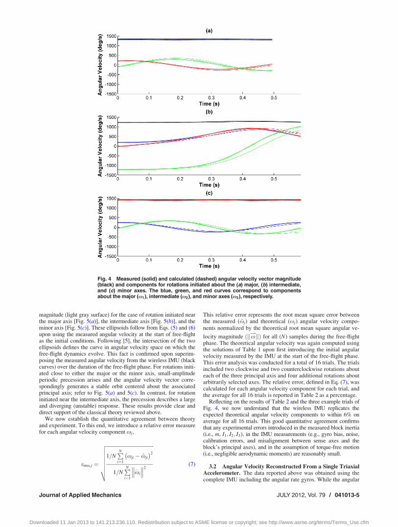
We now turn our attention to a detailed comparison of experi-mental and theoretical results for free-flight dynamics. Figure 4illustrates results for rotation initiated close to the major axis[Fig. 4(a)], the intermediate axis [Fig. 4(b)], and the minor axis[Fig. 4(c)]. In each case, experimental (solid) and theoretical(dashed) time histories are plotted for the three angular velocitycomponents as well as their vector magnitude (black). Recall thatthe components x1 (blue), x2 (green), and x3 (red) are alignedwith the major, intermediate, and minor axes, respectively. The

illustrated experimental data is low-pass filtered using a 100 Hzcut-off frequency to remove modest measurement noise. The theo-retical results are computed from the solutions reported in Table 1upon using the measured angular velocity at the start of free-flightas the initial condition for the remainder of the free-flight phase.

The results of Fig. 4 clearly confirm expected free-flight behav-iors. For rotation initiated near the major (minor) axis as illustratedin Fig. 4(a) [Fig. 4(c)], the block rotates in a stable manner with alarge, near-steady angular velocity component about the major(minor) axis. Moreover, the two “off-axis” components of angularvelocity remain small and exhibit small periodic oscillations. Theoscillation frequencies match those predicted by linear theory2 towithin 0.8% (8.3%) for the illustrated case of rotation about themajor (minor) axis. In contrast, for rotation initiated near the inter-mediate axis as illustrated in Figs. 4(b), the block experiencesunstable rotation as evidenced by the large, diverging precession.

The stable and unstable rotations are elegantly described geomet-rically upon construction of the associated polhodes as illustrated inFig. 5. Shown in this figure are the ellipsoids of constant rotationalkinetic energy (dark gray surface) and constant angular momentum

Fig. 3 Example time histories of the measured (a) magnitude of the accelerationof point P, (b) magnitude of the angular velocity, (c) the rotational kinetic energy,and (d) magnitude of angular momentum about center of mass. The throw, free-flight, and catch phases are noted. Example trial for rotation initiated nearly aboutthe minor axis.

1Note that the MEMS accelerometer detects acceleration down to DC and thus italso measures gravity.

2For example, refer to [4]. This classical analysis reveals that the “off-axis” com-ponents of angular velocity will oscillate with frequencyxn ¼ X

ffiffiffiffiffiffiffiffiffiffiffiffiffiffiffiffiffiffiffiffiffiffiffiffiffiffiffiffiffiffiffiffiffiffiffiffiffiffiffiffiffiffiffiffiI1 � I3ð Þ I2 � I1ð Þ=I3I2

por xn ¼ X

ffiffiffiffiffiffiffiffiffiffiffiffiffiffiffiffiffiffiffiffiffiffiffiffiffiffiffiffiffiffiffiffiffiffiffiffiffiffiffiffiffiffiffiffiI1 � I3ð Þ I3 � I2ð Þ=I1I2

pfor rotations

about the major and minor axes, respectively, where X is the magnitude of angularvelocity component about the major or minor axis.



magnitude (light gray surface) for the case of rotation initiated nearthe major axis [Fig. 5(a)], the intermediate axis [Fig. 5(b)], and theminor axis [Fig. 5(c)]. These ellipsoids follow from Eqs. (5) and (6)upon using the measured angular velocity at the start of free-flightas the initial conditions. Following [5], the intersection of the twoellipsoids defines the curve in angular velocity space on which thefree-flight dynamics evolve. This fact is confirmed upon superim-posing the measured angular velocity from the wireless IMU (blackcurves) over the duration of the free-flight phase. For rotations initi-ated close to either the major or the minor axis, small-amplitudeperiodic precession arises and the angular velocity vector corre-spondingly generates a stable orbit centered about the associatedprincipal axis; refer to Fig. 5(a) and 5(c). In contrast, for rotationinitiated near the intermediate axis, the precession describes a largeand diverging (unstable) response. These results provide clear anddirect support of the classical theory reviewed above.

We now establish the quantitative agreement between theoryand experiment. To this end, we introduce a relative error measurefor each angular velocity component xj,

erms;j ¼

ffiffiffiffiffiffiffiffiffiffiffiffiffiffiffiffiffiffiffiffiffiffiffiffiffiffiffiffiffiffiffiffiffiffiffiffiffiffiffi1=N

PNi¼1

xji � ~xji

� �2

1=NPNi¼1

x*

i

�� 2

vuuuuuut (7)

This relative error represents the root mean square error betweenthe measured ( ~xj) and theoretical (xj) angular velocity compo-nents normalized by the theoretical root mean square angular ve-

locity magnitude ðkx*kÞ for all (N) samples during the free-flightphase. The theoretical angular velocity was again computed usingthe solutions of Table 1 upon first introducing the initial angularvelocity measured by the IMU at the start of the free-flight phase.This error analysis was conducted for a total of 16 trials. The trialsincluded two clockwise and two counterclockwise rotations abouteach of the three principal axis and four additional rotations aboutarbitrarily selected axes. The relative error, defined in Eq. (7), wascalculated for each angular velocity component for each trial, andthe average for all 16 trials is reported in Table 2 as a percentage.

Reflecting on the results of Table 2 and the three example trials ofFig. 4, we now understand that the wireless IMU replicates theexpected theoretical angular velocity components to within 6% onaverage for all 16 trials. This good quantitative agreement confirmsthat any experimental errors introduced in the measured block inertia(i.e., m, I1; I2; I3), in the IMU measurements (e.g., gyro bias, noise,calibration errors, and misalignment between sense axes and theblock’s principal axes), and in the assumption of torque-free motion(i.e., negligible aerodynamic moments) are reasonably small.

3.2 Angular Velocity Reconstructed From a Single TriaxialAccelerometer. The data reported above was obtained using thecomplete IMU including the angular rate gyros. While the angular

Fig. 4 Measured (solid) and calculated (dashed) angular velocity vector magnitude(black) and components for rotations initiated about the (a) major, (b) intermediate,and (c) minor axes. The blue, green, and red curves correspond to componentsabout the major (x1), intermediate (x2), and minor axes (x3), respectively.



rate gyros yield highly accurate measurements of angular velocity,they are relatively expensive compared to the embedded triaxialaccelerometer. The addition of angular rate gyros obviously cre-ates a larger volume design. Moreover, commercial MEMS rategyros have limited range (e.g., typical ranges today are 6000 deg/sand less). Thus, the restrictions incurred by rate gyro cost, size,and measurement range may preclude their use in high-volumecommercial applications such as instrumented basketballs, soccerballs, baseballs, golf balls, footballs, softballs, and the like. Thisrealization naturally leads to the question of whether it is possibleto arrive at the same accurate measurements of angular velocitywithout the use of angular rate gyros for free-flight dynamics. Wepresent below an answer to this question beginning with the mea-surement theory and then proceeding to the experimentalevidence.

In reference to Fig. 2, the acceleration of point P (the center ofthe triaxial accelerometer) on the rigid body, can be written interms of the acceleration of the mass center C through

a*

p ¼ a*

c þ _x* � r

*

p=c þ x* � x

* � r*

p=c

� �(8)

where a*

c denotes the acceleration of the mass center, r*

p=c is again

the position of P relative to C, and x*

and_x*

are, respectively, theangular velocity and angular acceleration of the rigid body. Theacceleration measured by the MEMS accelerometer is the vectorsum of the acceleration of point P minus the acceleration due togravity [20] as given by

a*

s ¼ a*

p þ gK (9)

where g denotes gravity and K is a unit vector directed upwards.For the case of a rigid body in free-flight, the acceleration of themass center is simply

a*

c ¼ �gK (10)

assuming negligible aerodynamic drag. Substitution of Eqs. (9)and (10) into Eq. (8) yields

a*

s ¼ _x* � r

*

p=c þ x* � x

* � r*

p=c

� �(11)

Fig. 5 Experimental demonstration of the polhode for rotations initiated close tothe (a) major, (b) intermediate, and (c) minor principal axes. The measured angularvelocity during the entire free-flight phase (black, scale in deg/s), closely followsthe polhode defined by the intersection of the ellipsoids.

Table 2 Quantitative comparison of theoretical and experimen-tal angular velocity components. Relative root-means-squareerror for each angular velocity component averaged over all 16trials. The error measure is given by Eq. (7) and reported in thistable as a percentage.

j 1 2 3

erms;j %ð Þ 3.0 5.8 4.6



where it is obvious that the accelerometer output depends on therotational dynamics of the rigid body as governed by the torque-

free form of Euler’s equations. Solving Eq. (1) for_x*

and substitut-ing this result into Eq. (11) yields

a*

s ¼ �I�1c x

* � Icx*

� �h i� r

*

p=c þ x* � x

* � r*

p=c

� �(12)

which explicitly demonstrates that the output of the accelerometeralone can be used to deduce the angular velocity. Introducing the

components a*

s ¼ as1 as2 as3½ �T and r*

p=c ¼ r1 r2 r3½ �T into

Eq. (12) yields the component equivalent

as1

as2

as3

264

375 ¼

� x22 þ x2

3

� �1� Icð Þx1x2 1þ Ibð Þx1x3

1þ Icð Þx1x2 � x21 þ x2

3

� �1� Iað Þx3x2

1� Ibð Þx1x3 1þ Iað Þx3x2 � x21 þ x2

2

� �264

375

r1

r2

r3

264

375

(13a)

or

a*

s ¼ B x*� �

r*

p=c (13b)

in which Ia ¼ I2� I3ð Þ=I1, Ib ¼ I3� I1ð Þ=I2, and Ic ¼ I1� I2ð Þ=I3.Equation (13) provides three quadratic equations for solution ofthe three unknown angular velocity components from the meas-ured acceleration components of point P.

Moreover, the solution for x*

must satisfy the two constants ofthe motion given by Eqs. (2) and (3). These additional equations,though not independent of the above result that embeds Euler’sequations, are advantageous in the computation of x

*. In particu-

lar, Eq. (13) with Eqs. (2) and (3) yield an overdetermined set offive equations in the three unknowns (x1;x2;x3) enabling a ro-bust least squares solution, provided the values of the constants ofthe motion are known a priori.

To compute these constants, we first seek the initial conditionsfor the angular velocity and the two constants of the motion asrepresented by the set [x1 0ð Þ;x2 0ð Þ;x3 0ð Þ; 2T0;H

20]. To this end,

we numerically solve Eq. (13) with Eqs. (2) and (3) as a set of fiveequations in these five unknowns using the measured values of[as1 0ð Þ; as2 0ð Þ; as3 0ð Þ] at the start of the free-flight phase. This setof nonlinear equations admits multiple solutions which is a welldocumented issue; see for example [16,19,20,29,30]. The prob-lem, illustrated by Eq. (11), is that the expression for a

*

s is quad-ratic in x

*which renders the sign of the angular velocity vector

Table 3 Relative root-mean-square error for angular velocitycomponents reconstructed using a single, triaxial accelerome-ter as compared to those measured directly from the angularrate gyros

j 1 2 3

erms;j %ð Þ 1.3 1.2 1.2

Fig. 6 Measured (solid) and reconstructed (dashed) angular velocity magnitude(black) and components for rotations initiated nearly about the (a) major, (b) inter-mediate, and (c) minor axes. The blue, green, and red curves correspond to com-ponents about the major (x1), intermediate (x2), and minor axes (x3), respectively.



(though not the direction) ambiguous. The sign can be readilydetermined by simple observation during the experiment.

For any other time t during the free-flight phase, we computethe least-squares solution for x

*tð Þ from the five equations (13)

with (2) and (3). For each sample i, we seek the solution for x*

that minimizes the cost function

Ji ¼a*

s;i � B x*� �

r*

p=c

�� PNi¼1

a*

s;i

�� .N

0BBB@

1CCCA

2

þ 2T0 � 2Ti

2T0

2

þH2

0 � H*

i

�� 2

H20

0B@

1CA

2

(14)

where a*

s;i is the sampled accelerometer output, and N is the totalnumber of samples. The solution is found numerically using thelsqnonlin function in MATLAB

TM and angular velocity componentsfrom the last time step as an initial guess. The lsqnonlin functionemploys a trust-region method for numerical, unconstrained, non-linear, minimization problems [31].

The components of angular velocity, as reconstructed from a sin-gle triaxial accelerometer, reliably predict those measured by theangular rate gyros. Evidence for this claim is presented in Fig. 6which directly compares the reconstructed versus measured angularvelocity. Results are presented for three example trials where rota-tion is initiated nearly about the major [Fig. 6(a)], the intermediate[Fig. 6(b)], and the minor [Fig. 6(c)] axes. Both the angular velocitycomponents as well as the magnitude of the angular velocity vectorare illustrated. Inspection of these results reveals excellent agree-ment thereby demonstrating that a single, triaxial accelerometer canbe employed to accurately reconstruct the angular velocity duringfree-flight. The accuracy is summarized quantitatively in Table 3which reports the average relative rms error3 for the 16 trials previ-ously considered. The errors, which remain less than 2% for allthree angular velocity components, provide convincing evidence insupport of our claim.

4 Summary and Conclusions

The novel, miniature wireless MEMS IMU presented herein pro-vides a noninvasive and highly portable means to measure the dy-namics of a rigid body. The IMU incorporates three-axis sensing ofacceleration and three-axis sensing of angular velocity with a micro-controller and an RF transceiver for wireless data transmission to ahost computer. The small sensor footprint (0.019� 0.024 m) andmass (0.005 kg including battery) enables its use in rather broadapplications including; for example, human motion analysis, sportstraining systems, and education/learning of rigid body dynamics.Specific to this paper, we demonstrate how this novel sensor can beused in laboratory or classroom settings to accurately measure thedynamics of a rigid body in free-flight.

The experiments consider an example rigid body that is spun upby hand and then released into free-flight. The resulting rotationaldynamics measured by the angular rate gyros are carefully bench-marked against theoretical results from Euler’s equations. Thiscomparison reveals that differences between measurement andtheory remain less than 6%. Moreover, experimentally con-structed polhodes elegantly illustrate the expected stable preces-sion for rotations initiated close to the major or minor principalaxes and the unstable precession for rotations initiated close to theintermediate axis.

Finally, we present a single, triaxial accelerometer as an alterna-tive to using a full IMU for deducing the angular velocity of a rigidbody during free-flight. This simpler alternative, which addressesrestrictions incurred by rate gyro cost, size, and measurement range,may enable high-volume commercial applications such as instru-

mented basketballs, soccer balls, baseballs, golf balls, footballs,softballs, and the like. A measurement theory is presented forreconstructing the angular velocity of the body during free-flightfrom acceleration signals which is then validated experimentally.The experimental results confirm that the angular velocity can bereconstructed with small errors (less than 2%) when benchmarkedagainst direct measurements using angular rate gyros.

Acknowledgment

The authors gratefully acknowledge past support from the Uni-versity of Michigan Graduate Medical Education InnovationsFund and from Ebonite International for the development of thewireless IMU. The first author also gratefully acknowledges sup-port provided by a National Science Foundation Graduate StudentFellowship.

References[1] Routh, E. J., 1860, Dynamics of a System of Rigid Bodies, 6th ed., MacMillan,

New York.[2] Gray, A., 1918, Treatise on Gyrostatics and Rotational Motion, MacMillan,

London.[3] Goldstein, H., 1922, Classical Mechanics, 2nd ed., Addison-Wesley, Reading,

MA.[4] Greenwood, D. T., 1988, Principles of Dynamics, Prentice-Hall, Englewood

Cliffs, NJ.[5] Wie, B., 1998, Space Vehicle Dynamics and Control, American Institute of

Aeronautics and Astronautics, Reston, VA.[6] Mettler, B. F., 2010, “Extracting Micro Air Vehicles Aerodynamic Forces and

Coefficients in Free Flight Using Visual Motion Tracking Techniques,” Exp.Fluid Mech., 49, pp. 577–569.

[7] Aghili, F., and Parsa, K., 2009, “Motion and Parameter Estimation of SpaceObjects Using Laser Vision Data,” J. Guidance Control Dyn., 32(2), pp.537–549.

[8] Lichter, M. D., and Dubowsky, S., 2004, “State, Shape, and Parameter Estima-tion of Space Objects from Range Images,” Proceedings of the 2004 IEEEInternational Conference on Robotics & Automation, New Orleans, LA, pp.2974–2979.

[9] Hillenbrand, U., and Lampariello, R., 2005, “Motion and Parameter Estimationof a Free-Floating Space Object from Range Data for Motion Prediction,” 8thInternational Symposium on Artificial Intelligence, Robotics, and Automationin Space.

[10] Kim, S.-G., Crassidis, J. L. Cheng, Y. Fosbury, A. M., and Junkins, J. L., 2007,“Kalman Filtering for Relative Spacecraft Attitude and Position Estimation,” J.Guidance Control Dyn., 30(1), pp. 133–143.

[11] Thienel, J. K., and Sanner, R. M., 2007, “Hubble Space Telescope Angular Ve-locity Estimation During the Robotic Servicing Mission,” J. Guidance ControlDyn., 30(1), pp. 29–34.

[12] Bhat, K. S., Seitz, S. M., Popovic, J., and Khosla, P. K., 2002, “Computing thePhysical Parameters of Rigid-Body Motion from Video,” Lecture Notes inComputer Science, 2350, pp. 551–565.

[13] Masutani, Y., Iwatsu, T., and Miyazaki, F., 1994, “Motion Estimation ofUnknown Rigid Body Under No External Forces and Moments,” Proceedingsof IEEE International Conference on Robotics and Automation 1994, IEEEComputer Society Press, New York, Vol. 2, pp. 1066–1072.

[14] Lorenz, R. D., 2005, “Flight and Attitude Dynamics Measurements of an Instru-mented Frisbee,” Meas. Sci. Technol., 16, pp. 738–748.

[15] Titterton, D., and Weston, J., 2004, Strapdown Inertial Navigation Technology,2nd ed., The Institution of Electrical Engineers, Stevenage, Herts, UK.

[16] Zappa, B., Legnani, G., van den Bogert, A., and Adamini, R., 2001, “On theNumber and Placement of Accelerometers for Angular Velocity and Accelera-tion Determination,” ASME J. Dyn. Syst. Meas. Control, 123, pp. 552–554.

[17] Cardou, P., and Angeles, J., 2008, “Angular Velocity Estimation From theAngular Acceleration Matrix,” ASME J. Appl. Mech., 75(2), p. 021003.

[18] Mital, N. K., and King, A. I., 1979, “Computation of Rigid-Body Rotation inThree-Dimensional Space from Body-Fixed Linear Acceleration Meas-urements,” ASME J. Appl. Mech., 46, pp. 925–930.

[19] Genin, J., Hong, J., and Xu, W., 1997, “Accelerometer Placement for AngularVelocity Determination,” ASME J. Dyn. Syst. Meas. Control, 119(3), pp.474–477.

[20] Chen, J., Lee, S., and DeBra, D. B., 1994, “Gyroscope Free Strapdown InertialMeasurement Unit by Six Linear Accelerometers,” J. Guidance Control Dyn.,17(2), pp. 286–290.

[21] Hanson, R., and Pachter, M., 2005, “Optimal Gyro-Free IMU Geometry,”AIAA Guidance, Navigation, and Control Conference and Exhibit 15–18 Au-gust 2005, San Francisco, CA.

[22] King, K. W., 2008, “The Design and Application of Wireless MEMS InertialMeasurement Units for the Measurement and Analysis of Golf Swings,” Ph.D.Thesis, University of Michigan, Ann Arbor, MI.

[23] King, K. W., and Perkins, N. C., 2008, “Putting Stroke Analysis Using MEMSInertial Sensor Systems,” World Scientific Congress on Golf V, Phoenix, AZ,pp. 270–278.

3The error measure is again given by (7) where the angular velocity measured bythe angular rate gyros is now used as the “truth” data.



http://dx.doi.org/10.2514/1.37129

http://dx.doi.org/10.2514/1.22377

http://dx.doi.org/10.2514/1.22377

http://dx.doi.org/10.2514/1.20591

http://dx.doi.org/10.2514/1.20591

http://dx.doi.org/10.1007/3-540-47969-4_37

http://dx.doi.org/10.1007/3-540-47969-4_37

http://dx.doi.org/10.1088/0957-0233/16/3/017

http://dx.doi.org/10.1115/1.1386649

http://dx.doi.org/10.1115/1.2775495

http://dx.doi.org/10.1115/1.3424679

http://dx.doi.org/10.1115/1.2801281

http://dx.doi.org/10.2514/3.21195

[24] King, K. W., Yoon, S. W., Perkins, N. C., and Najafi, K., 2004, “The Dynamicsof the Golf Swing as Measured by Strapdown Inertial Sensors,” Proceedings5th International Conference on the Engineering of Sport, Davis, CA, pp.276–282.

[25] King, K. W., Yoon, S. W., Perkins, N. C., and Najafi, K., 2008, “WirelessMEMS Inertial Sensor System for Golf Swing Dynamics,” Sensors ActuatorsA, 141(2), pp. 619–630.

[26] Perkins, N. C., 2007 and 2006, “Electronic Measurement of the Motion of a Mov-ing Body of Sports Equipment,” US Patent Numbers 7,234,351 and 7,021,140.

[27] Kane, T. R., Likins, P. W., and Levinson, D. A., 1983, Spacecraft Dynamics,McGraw-Hill, New York.

[28] van Zon, R., and Schofield, J., 2007, “Numerical Implementation of the ExactDynamics of Free Rigid Bodies,” J. Comput. Phys., 225(1), pp. 145–164.

[29] Williams, T., Pahadia, A., Petovello, M., and Lachapelle, G., 2009, “Using anAccelerometer Configuration to Improve the Performance of a MEMS IMU:Feasibility Study With a Pedestrian Navigation Application,” ION GNSS 2009,Session F4, Savannah, GA.

[30] Ciblak, N., 2007, “Determining the Angular Motion of a Rigid Body Using Lin-ear Accelerometers Without Integration,” 3rd International Conference onRecent Advances in Space Technologies. RAST ’07, pp. 585–590.

[31] More, J. J., and Sorensen, D. C., 1983, “Computing a Trust Region Step,”SIAM J Sci. Comput., 4(3), pp. 553–572.



http://dx.doi.org/10.1016/j.sna.2007.08.028

http://dx.doi.org/10.1016/j.sna.2007.08.028

http://dx.doi.org/10.1016/j.jcp.2006.11.019

http://dx.doi.org/10.1137/0904038

reconstructing free-flight angular velocity from a ...ryanmcg/updated documents 11-9...and yields...

Documents