1

Reconstructing fiber networks from confocal image stacksPatrick Krauss, Claus Metzner∗, Janina Lange, Nadine Lang, Ben FabryDept. of Physics, Biophysics Group, Friedrich-Alexander University, Erlangen, Germany∗ E-mail: claus.metzner@gmx.net

Abstract

We present a numerically efficient method to reconstruct a disordered network of thin biopolymers, suchas collagen gels, from three-dimensional (3D) image stacks recorded with a confocal microscope. Ourmethod is based on a template matching algorithm that simultaneously performs a binarization andskeletonization of the network. The size and intensity pattern of the template is automatically adaptedto the input data so that the method is scale invariant and generic. Furthermore, the template matchingthreshold is iteratively optimized to ensure that the final skeletonized network obeys a universal propertyof voxelized random line networks, namely, solid-phase voxels have most likely three solid-phase neighborsin a 3 × 3 neighborhood. This optimization criterion makes our method free of user-defined parametersand the output exceptionally robust against imaging noise.

Introduction

Many biological materials, such as the cytoskeleton or the extracellular matrix, self-organize into complexnetworks by the polymerization of protein molecules into fibrils (Fig. 1). If the thickness of the fibrilsis negligible compared to the pore size, the resulting structure can be mathematically described as adisordered line network. In general, the functional properties of these networks, such as their mechanicalstiffness on the macroscopic scale, or their permeability for diffusing particles and for actively migratingcells on a microscopic scale, depend on the geometrical details of the microscopic network structure.In order to study the relationship between structure and function, it is therefore important to extract,or reconstruct, the 3D network structure from image stacks. One aspect of the reconstruction is thebinarization of the intensity values of the image stack, so that each voxel is assigned one of two possiblevalues, corresponding either to the solid phase (1, collagen fibers) or the liquid phase (0, surroundingmedium). Another aspect of the reconstruction is the skeletonization, so that the optically broadenedfibers are reduced to their central (medial) axis, with a width of only one voxel.

While most of the standard reconstruction methods realize the two aspects of reconstruction (i.e.binarization and skeletonization) in a two-step process, our template matching method achieves bothaspects in a single step. This new method avoids the problem of chosing an arbitrary intensity thresholdfor the binarization. Instead, the template matching algorithm automatically adapts to the input datasuch that within the reconstructed fraction of solid-phase voxels the most probable number of nextneighbors equals three. This represents a universal property of voxelized line networks.

Criteria for reconstruction methods We regard it essential to define the following criteria forour reconstruction method: (1) The method needs to be free of user-adjustable parameters, and (2) beinsensitive to variations in the input data quality. To test this criterion we image collagen networks undera wide range of different confocal microscope settings such as amplifyer gain and laser outlet power. Themethod (3) must be able to correctly reconstruct known networks. To simulate realistic conditions, thesenetworks are convoluted with a point spread function of the imaging system, and different levels of noiseare added.

Existing reconstruction methods A vast variety of methods can be used for the reconstructionproblem. A large class of these methods works with two separate steps of binarization and skeletonization

arX

iv:1

111.

3861

v1 [

q-bi

o.Q

M]

16

Nov

201

1

2

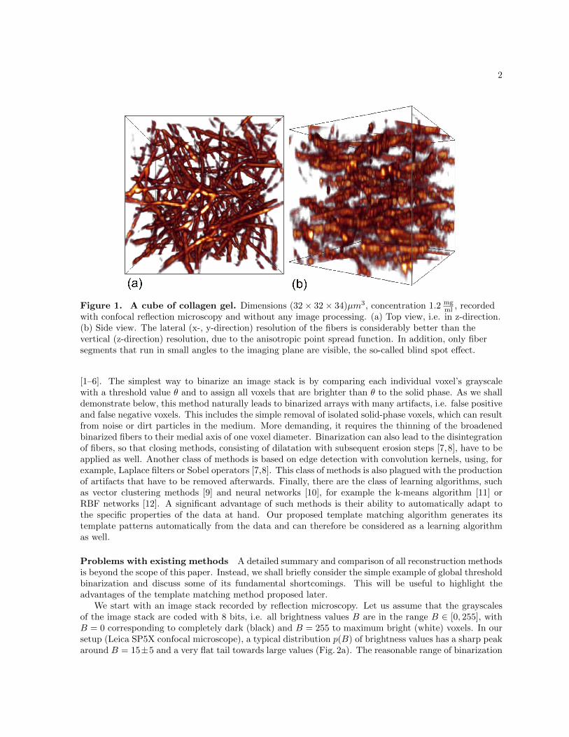
Figure 1. A cube of collagen gel. Dimensions (32× 32× 34)µm3, concentration 1.2 mgml , recorded

with confocal reflection microscopy and without any image processing. (a) Top view, i.e. in z-direction.(b) Side view. The lateral (x-, y-direction) resolution of the fibers is considerably better than thevertical (z-direction) resolution, due to the anisotropic point spread function. In addition, only fibersegments that run in small angles to the imaging plane are visible, the so-called blind spot effect.

[1–6]. The simplest way to binarize an image stack is by comparing each individual voxel’s grayscalewith a threshold value θ and to assign all voxels that are brighter than θ to the solid phase. As we shalldemonstrate below, this method naturally leads to binarized arrays with many artifacts, i.e. false positiveand false negative voxels. This includes the simple removal of isolated solid-phase voxels, which can resultfrom noise or dirt particles in the medium. More demanding, it requires the thinning of the broadenedbinarized fibers to their medial axis of one voxel diameter. Binarization can also lead to the disintegrationof fibers, so that closing methods, consisting of dilatation with subsequent erosion steps [7,8], have to beapplied as well. Another class of methods is based on edge detection with convolution kernels, using, forexample, Laplace filters or Sobel operators [7,8]. This class of methods is also plagued with the productionof artifacts that have to be removed afterwards. Finally, there are the class of learning algorithms, suchas vector clustering methods [9] and neural networks [10], for example the k-means algorithm [11] orRBF networks [12]. A significant advantage of such methods is their ability to automatically adapt tothe specific properties of the data at hand. Our proposed template matching algorithm generates itstemplate patterns automatically from the data and can therefore be considered as a learning algorithmas well.

Problems with existing methods A detailed summary and comparison of all reconstruction methodsis beyond the scope of this paper. Instead, we shall briefly consider the simple example of global thresholdbinarization and discuss some of its fundamental shortcomings. This will be useful to highlight theadvantages of the template matching method proposed later.

We start with an image stack recorded by reflection microscopy. Let us assume that the grayscalesof the image stack are coded with 8 bits, i.e. all brightness values B are in the range B ∈ [0, 255], withB = 0 corresponding to completely dark (black) and B = 255 to maximum bright (white) voxels. In oursetup (Leica SP5X confocal microscope), a typical distribution p(B) of brightness values has a sharp peakaround B = 15±5 and a very flat tail towards large values (Fig. 2a). The reasonable range of binarization

3

thresholds θ is located somewhere within this tail. However, the distribution p(B) itself offers no hint asto where the optimum threshold point should be set.

To characterize different network reconstruction methods, we use artificially generated image stacks.This requires realistic models of both, the line network itself and its transformation into cross-sectionalimages by the microscope. As described in more detail in the Methods section, we use a ”Mikado”model for the line network, where straight lines of fixed lengths and isotropic orientations are distributedthroughout the volume with a homogeneous density [13]. To model the imaging process, we take intoaccount the broadening (simulated by a convolution with a point spread function), the blind spot effect(i.e. a gradual darkening of steep fibers) [14] and the addition of random noise. The resulting imagestacks have statistical properties almost indistinguishable from measured image stacks (Fig. 2), but withthe advantage that the underlying mathematical line network is known precisely.

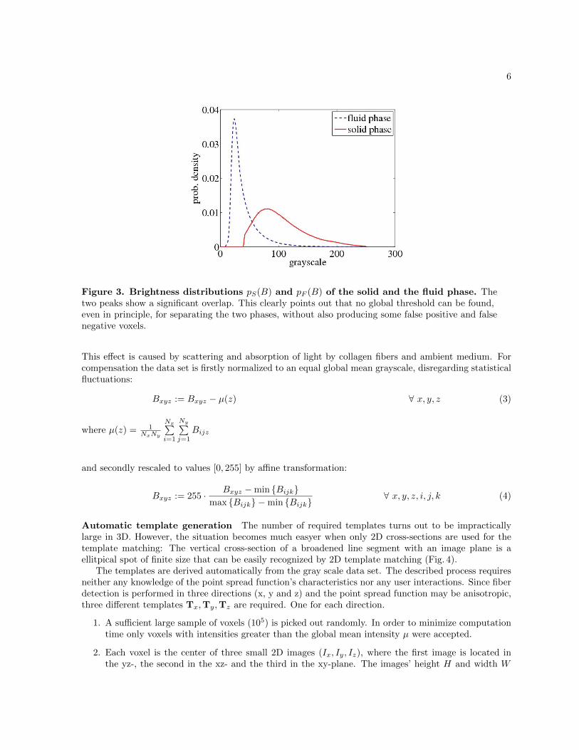
Is it possible to perfectly reconstruct the original line network using global threshold binarization?This would require the existence of a threshold θ, such that all fluid-phase voxels have brightnesses belowand all solid-phase-voxels brightnesses above this threshold. However, when we use our synthetic stackand plot the brightness distributions pS(B) and pF (B) of the two phases separately, we find in generaltwo peaks with a significant overlap (Fig. 3). This means that no global threshold can be found, evenin principle, for separating the two phases, without also producing some false positive and false negativevoxels.

The voxels with brightnesses in the overlap interval include, for example, isolated bright points dueto noise. It would be relatively easy to remove such cases in a subsequent post-processing step. Moreproblematic is that the overlap interval also includes liquid phase voxels from the narrow gaps betweentwo fibers, which have been raised in brightness beyond the threshold by the superposition of the fibers’point spread functions. This effect would lead to a merging of the two close-by fibers in the binarizedimage and would require a much more sophisticated procedure to be repaired. Finally, the overlap regionincludes voxels of fiber segments that are more vertically oriented, and therefore too dark, to exceed thethreshold, because of the blind spot problem [14]. We note that a human observer could still recognizesuch dark fiber segments quite easily.

Taken together, the threshold binarization has some fundamental limitations. To a certain extent,the method can be improved by using variable thresholds, which take into account the local brightnessconditions in the environment of each voxel to be binarized. This, however, can already be viewed as afirst step towards a template matching method that will be discussed in the following.

Template matching in line networks Template matching methods recognize specific image partswithin larger image stacks by comparing features, e.g. the brightness patterns, of small sub volumes ofthe stack with the brightness pattern of pre-defined templates. The templates incorporate the a-priori-knowledge about the features to be found. In the case of line networks, the templates would containshort line segments, that are oriented in arbitrary directions.

The number of required templates turns out to be impractically large in 3D. However, the situation ismuch simpler when only 2D cross-sections are used for the template matching: The vertical cross-sectionof a broadened line segment with a plane is a elliptical spot of finite size that can be easily recognizedby 2D template matching (Fig. 4a). The shape of the spot will vary slightly as the angle of intersectionbecomes less than 90 degrees. For angles less than 45 degrees, the distortion of the spot can become toolarge to match the template (Fig. 4b), but in this case the same line segment can be easily recognized byits intersection with a perpendicular plane. Therefore, all line segments (solid voxels) can be detectedby sequentially scanning through the x-, y- and z-planes of the sample volume. As shown below thisbinarization method turns out to be much more reliable and robust than the simple threshold method.

The similarity between the cross-sectional brightness pattern and the template will be largest if thetemplate is located exactly at the center of the finite spot. Therefore, the medial axes of the broadenedline segments can be identified as local minima of the mismatching measure. In this way, the 2D template

4

matching simultaneously achieves a skeletonization of the broadened fibers.We note that this method meets the design criteria imposed before. In order to eliminate all internal

parameters (1), we have implemented an automatic template generator, which is entirely based on theinput image stack and requires no user intervention. We will demonstrate in the Results section that ourmethod is also robust with respect to the quality of the input data (2) and yields reconstructions thatreproduce simulated line networks almost perfectly (3). The algorithm is implemented in C++ to achievefast execution times (about 12 minutes on a standard notebook for reconstructing a (512×512×597)-voxelstack) and is available as a supplement to this publication.

Methods

Generation of surrogate data sets Since the true shape of the underlying fiber network of realgrayscale data sets is unknown, we artificially generated surrogate data sets to validate the performanceof our algorithm. Firstly we created idealized line networks using a ”Mikado” model. Straight linesof fixed lengths and isotropic orientations are distributed throughout the volume with a homogeneousdensity [13]. Binary surrogate data sets are derived from these parameterized networks by a voxelizationoperation. Then we simulate the imaging process to transform these binary data sets into grayscale datasets.

Initially N sets of parameters representing N lines are randomly generated. Each parameter set con-tains uniformly distributed Cartesian coordinates of a line’s center point (xc, yc, zc), uniformly distributedazimuthal angle ϕ ∈ [−π, π] with p(ϕ) = 1

2π and polar angle ϑ ∈ [0, π] with p(ϑ) = sinϑ2 . This is an

efficient way of representing a line network, since for each arbitrary point within the volume one canunambiguously determine whether or not the point is located on any line.

To derive a binary data set from the parameterized network the whole volume is divided into distinctvolume elements representing the voxels. Initially all voxels within the 3D-array are set to value 0(fluid phase). Starting at the first center point, the line is traced in opposite directions according to itsorientation (ϕ, ϑ) until the half length of the line is reached for each direction. While tracing the line,every voxel corresponding to a touched volume element is set to value 1 (solid phase). This process isrepeated for all N sets of line parameters.

To convert the binary data set into a 8-bit-grayscale data set, we apply a process called numericblurring which simulates the imaging process. Numeric blurring is done in five subsequent steps:

1. The binary 3D-array of voxels is converted into a grayscale 3D-array by setting all voxels with value1 to brightness values B ∈ [0, 255] according to the polar angle ϑ of the line to which they belong.This procedure replicates the blind spot effect (i.e. a gradual darkening of steep fibers) as describedin [14].

2. A small number of dark voxels is randomly selected and set to brightness values > 200. Thissimulates dirt particles within the fluid phase that appear as isolated bright fluctuations in theoriginal microscope images.

3. The 3D-array of voxels is convoluted with an anisotropic Gaussian to simulate the point spreadfunction:

B(x, y, z) := (B ∗ psf)(x, y, z) (1)

(B ∗ psf)(x, y, z) =

∫∫∫B(x′, y′, z′)psf(x− x′, y − y′, z − z′)dx′ dy′ dz′ (2)

where B(x, y, z) ∈ [0, 255] is brightness of voxel (x, y, z). The point spread function is defined as

psf(x− x′, y − y′, z − z′) = exp(−(

(x−x′)2

σ2x

+ (y−y′)2σ2y

+ (z−z′)2σ2z

))with σx = σy < σz according to

the characteristics of confocal microscopy.

5

4. A Gaussian distributed random variable is added to each voxel to simulate noise1.

5. Finally, all brightness values are rescaled to values from 0 to 255 by affine transformation.

We have analyzed the statistical properties of the resulting grayscale data sets2. They are almostindistinguishable from real data sets imaged with confocal reflection microscopy (Fig. 2), but with theadvantage that the underlying mathematical line network is known in detail.

Figure 2. Statistical properties of real and surrogate image stacks. (a) Comparison of thebrightness distributions in the real and surrogate image stacks. Both distributions are similar. (b) and(c) show angular distributions of the fiber segments. (b) Typical distributions of azimuthal angles ϕ in areal and a surrogate data set. The distributions are almost indistinguishable. The peaks are a result ofvoxelization. The principal directions, corresponding to the x- and y-direction, as well as the principaldiagonals are over-represented in short fiber segments and lead to maxima at ϕ = 0,±π4 ,±

π2 ,±

3π4 ,±π.

(c) Typical distributions of polar angles ϑ in a real and a surrogate data set. Again, the distributionsare similar. Compared to an ideal isotropic network with p(ϑ) ∝ sin(ϑ), polar angles smaller than π

2 areincreasingly suppressed due to the blind spot effect of confocal reflection microscopy [14].

When we plot the brightness distributions pS(B) and pF (B) of the two phases (solid and fluid)separately, we find in general two peaks with a significant overlap (Fig. 3). This means that no globalthreshold can be found, even in principle, for separating the two phases, without also producing somefalse positive and false negative voxels.

Preprocessing Some data sets show a z-dependence of mean grayscale. The average brightness ofeach z-slice µ(z) is not constant in all layers, but rather decreases for deeper located slices in the stack.

1We are aware that photon shot noise would not be normally distributed. However, as shown below, the resultingstatistical properties of the surrogate stacks agree almost perfectly with measured data.

2It is possible to determine the direction vector of a short fiber segment, even from its voxelized representation, bytreating the brightness distribution as a mass distribution, computing and diagonalizing the moment of inertia tensor, andfinding the principal component axis of mimimal inertia. This principal component corresponds to the direction of thelocally straight line segment. Several conditions have to be met when analyzing a given small test volume: First, the fluidbackground of the fiber segment in the test volume should have a much smaller (ideally zero) brightness/mass than the fiberitself. It is therefore advisable to use already reconstructed stacks for this analysis. Second, the test volume should containenough solid voxels to clearly define a single fiber segment. Third, the test volume should not be so large to contain severalline-like objects with different directions. We have therefore used the following method: A number of PMX=105 sphericaltest volumes of radius r=3.0 vu (voxel unit, i.e. linear size of a single voxel) have been chosen randomly throughout thereconstructed stack, ensuring that each test volume contains at least NMIN=5 solid voxels. Inside each sphere, the voxelswere treated as mass points, located at the voxel centers, and with constant mass m=1 for all solid and m=0 for all liquidvoxels. After determining the easy axis of the inertia tensor, the corresponding unit direction vector was computed. Notethat this vector does not depend on the exact position of the test sphere’s center, as long as the same solid voxels areenclosed. From this Cartesian vector, the azimuthal angle ϕ and the polar angle ϑ in spherical coordinates were computed.Finally, histograms were generated for ϕ and ϑ.

6

Figure 3. Brightness distributions pS(B) and pF (B) of the solid and the fluid phase. Thetwo peaks show a significant overlap. This clearly points out that no global threshold can be found,even in principle, for separating the two phases, without also producing some false positive and falsenegative voxels.

This effect is caused by scattering and absorption of light by collagen fibers and ambient medium. Forcompensation the data set is firstly normalized to an equal global mean grayscale, disregarding statisticalfluctuations:

Bxyz := Bxyz − µ(z) ∀ x, y, z (3)

where µ(z) = 1NxNy

Nx∑i=1

Ny∑j=1

Bijz

and secondly rescaled to values [0, 255] by affine transformation:

Bxyz := 255 · Bxyz −min {Bijk}max {Bijk} −min {Bijk}

∀ x, y, z, i, j, k (4)

Automatic template generation The number of required templates turns out to be impracticallylarge in 3D. However, the situation becomes much easyer when only 2D cross-sections are used for thetemplate matching: The vertical cross-section of a broadened line segment with an image plane is aellitpical spot of finite size that can be easily recognized by 2D template matching (Fig. 4).

The templates are derived automatically from the gray scale data set. The described process requiresneither any knowledge of the point spread function’s characteristics nor any user interactions. Since fiberdetection is performed in three directions (x, y and z) and the point spread function may be anisotropic,three different templates Tx,Ty,Tz are required. One for each direction.

1. A sufficient large sample of voxels (105) is picked out randomly. In order to minimize computationtime only voxels with intensities greater than the global mean intensity µ were accepted.

2. Each voxel is the center of three small 2D images (Ix, Iy, Iz), where the first image is located inthe yz-, the second in the xz- and the third in the xy-plane. The images’ height H and width W

7

Figure 4. 2D cross-section of a 3D image stack. (a) The vertical cross-section of a broadened linesegment with a plane is a elliptical spot of finite size that can be easily recognized by 2D templatematching. (b) The shape of the spot is varying slightly as the angle of intersection becomes less than 90degrees. For angles less than 45 degrees, the distortion of the spot can become too large to match thetemplate.

are initially set to arbitrary small values. The adaptive resizing process is described in a followingsection.

3. These small images are represented as H ×W matrices P1,P2, . . . ,PN , with matrix entries corre-sponding to voxel brightnesses. Hence three sets of training patterns {Px

i } , {Pyi } , {Pz

i } are obtainedto compute the three different templates.

4. From all training patterns belonging to a set, the weighted average pattern A is computed:

A :=

∑i

wiPi∑i

wi(5)

where wi is the central entry of matrix Pi.

5. To become independent from absolute brightnesses the global mean gray scale µ is subtracted fromeach matrix entry.

6. Finally the matrices Ax,Ay,Az are normalized to obtain the templates Tx,Ty,Tz:

T :=1

‖A‖A (6)

Fiber detection process As previously mentioned the fiber detecting process in the gray scale inputdata set is performed subsequently for all three directions x, y and z. During these three cycles threetemporary binary output data sets Ox,Oy,Oz are obtained, having each voxel labeled with one of two

8

possible values 0 (fluid phase) or 1 (collagen phase). The similarity between a given cross-sectionalbrightness pattern and the corresponding template will be largest if the template is located exactly atthe center of the finite spot. Therefore, the medial axes of the broadened line segments can be identifiedas local minima of the mismatching measure. The fiber detection process includes the following steps:

1. Initially all voxels of the first x-slice (yz-plane) with brightnesses larger than the mean gray scaleµ are investigated. This restriction is only made to decrease computation time. Without thisrestriction the fraction of additionally detected fiber voxels is less than 10−5. This small fractionis negligible since it does not significantly affect the resulting network properties on the one hand.On the other hand, performance time would be increased drastically by a factor of 5, because 80%of all voxels are darker than the mean brightness. Consequently all voxels with gray scales smallerthan µ are set to 0 in the binarized output data set Ox.

2. The voxels to be investigated are taken as centers of small 2D-images located in the yz-plane.These images are represented as matrices with the same size as the corresponding template. Thesematrices are the unknown patterns to be compared with the template. We call them search patternsSn.

3. From each entry of Sn the local mean value µn is subtracted.

4. The search patterns are normalized:

Sn :=1

‖Sn‖Sn (7)

5. Now the mismatch dn between search patterns Sn and template pattern Tx for detection in x-direction is computed. The smaller dn, the more probable the central voxel of the search patternbelongs to the collagen phase. As mismatch measuring metric we chose the Euclidean distance infeature space. Hence we call dn the matching distance.

dn := ‖Sn −Tx‖ =

√∑i

∑j

(snij − txij

)2(8)

Since all matrices are normalized, the range of dn is [0, 2] where dn = 0 means perfect matching.

6. The calculated matching distances dn are compared with the threshold θxd . This threshold defineswhether the search pattern is sufficiently similar to the template, so the pattern’s central voxelmay be a fiber voxel. For dn > θxd the corresponding voxels in Ox are set to 0. Note that allthresholds θxd , θ

yd , θ

zd are not chosen arbitrarily, but derived adaptively from the input data. The

detailed method of defining these thresholds will be described in a later section.

7. To all voxels being considered (dn < θxd) a local minimum filter is applied, labeling only local bestmatching voxels as belonging to collagen phase by assigning the value 1, while all others are setto 0. After having finished this step the first x-slice (yz-plane) of the input data set is completelybinarized and stored in the temporary binary output data set Ox.

8. All previous steps are repeated for all other x-slices resulting the first binarized data set Ox.

9. Some fibers with angles less than 45 degrees to any yz-plane (x-slice) may be not well detectedsince their cross-sections, appearing as roundish spots of finite size, are distorted and hence arenot sufficiently similar to the template. Therefore the complete detection process is repeated inperpendicular xz- and xy-planes (y- and z-slices) of the sample volume. Having all y- and z-slicesbinarized two more binary data sets Oy and Oz are obtained.

9

10. Finally the three temporary reconstruction results are combined to one binary data set using logicalOR:

Oijk := Oxijk ∨Oyijk ∨O

zijk ∀ i, j, k (9)

11. As a post-processing step all isolated voxels (i.e. solid phase voxels with all 26 neighbors belongingto fluid phase) are converted to fluid phase.

Define optimal template sizes The right size H ×W of the template T ∈ RH×W is crucial. On theone hand the template must not be too small, because otherwise the pattern is not completely covered.On the other hand templates should not be too large to limit computation time. A good indication isgiven by the algebraic sign of template’s matrix entries. Since all entries are reduced by subtracting themean gray scale µ, positive entries correspond to gray scales brighter than and vice versa negative entriesto gray scales darker than the average. Taking into account that the patterns to be detected are resultingfrom convolution of bright fibers with the point spread function it is reasonable to consider positivematrix entries as belonging to the pattern’s foreground, while negative entries represent the surroundingbackground. Hence, if the template is sized in a kind that all outer entries are negative and at the sametime all inner entries are positive it is warranted that the pattern is completely covered by the template.Furthermore using both, positive and negative matrix entries, implies better use of the complete domainof definition and contrast enhancement since matching distances dn only will be minimal if the templateis perfectly centered at the patterns being investigated.

Initially height H and width W are set to arbitrary, small values, e.g. H = 15 and W = 9. Then thetemplates are iteratively resized and recalculated until the optimal size is found. Since computing thetemplate takes only a few seconds the complete runtime is not affected significantly by these iterations.

Define optimal matching thresholds The optimal thresholds θxd , θyd and θzd are also defined itera-tively. It is clear that it depends on the thresholds how many voxels are labeled as fiber voxels. Becauseboth templates and search matrices are normalized the maximum range of matching distances dn is [0, 2]and consequently the optimal thresholds are in the same range as well.If matrices are treated as vectors in high-dimensional feature space, three special cases can be distin-guished:

Identity dn = 0 ⇒ Sn ≡ T

Orthogonality dn =√

2 ⇒ Sn ⊥ T

Inversion dn = 2 ⇒ Sn = −T

Where orthogonality means a maximum dissimilarity between template and search matrix. Inversionimplies identical absolute values of corresponding matrix entries with inverted algebraic signs. Hence[√

2, 2]

is no expedient range for the thresholds which rather must be within[0,√

2].

Since reconstructed fibers should be skeletonized, the most probably number of direct fiber voxelneighbors Emode in a 33-neighborhood of a central fiber voxel turns out to be a good criterion. Extensiveevaluations of simulated line networks showed Emode = 3 in case of perfect skeletonization.

Obviously there is not only a single value for thresholds that achieves Emode = 3, but rather a range,where the optimal thresholds would be the top of this range, because this causes a maximum number ofdetected fibers while simultaneously the constraint Emode = 3 is fulfilled.The threshold for each reconstruction direction x, y and z is defined in two subsequent steps. Firstlya threshold that fulfills Emode = 4 is found using a binary search algorithm. And secondly the foundthreshold is reduced step by step until it fulfills Emode = 3.

10

Binary Search Binary search is an efficient standard algorithm for searching a specified value byhalving the number of items to check with each iteration [15, 16]. Initially the threshold is set to themiddle of the range to be searched

[0,√

2]θ(0)d :=

0 +√

2

2=

1√2

(10)

and the bounds are defined

θmax(0)d :=

√2 (11)

θmin(0)d := 0 (12)

Then the following steps are repeated until the stop criterion is fulfilled:

1. The fiber detection algorithm is performed with recent threshold θ(n)d . To limit computation time

not the complete data set (containing 512×512×597 voxels) is used but a smaller sub set containingonly 150× 150× 150 voxels.

2. The most probable number of fiber voxel neighbors Emode is evaluated.

3. The threshold and the bounds of the searching range are updated:If Emode < 4 then:

θmax(n+1)d := θ

max(n)d (13)

θmin(n+1)d := θ

(n)d (14)

θ(n+1)d := (θ

max(n+1)d + θ

min(n+1)d )/2 (15)

If Emode > 4 then:

θmax(n+1)d := θ

(n)d (16)

θmin(n+1)d := θ

min(n)d (17)

θ(n+1)d := (θ

max(n+1)d + θ

min(n+1)d )/2 (18)

If Emode = 4 then binary search is stopped.

Reduction of threshold The threshold is now iteratively reduced until Emode = 3:

1. The fiber detection algorithm is performed using the recent threshold θ(n)d . Again due to limit

computation time not the complete data set is used but a sub set. However containing now morevoxels (i.e. 250× 250× 250) than previously used for binary search to increase accuracy.

2. The most probably number of fiber voxel neighbors Emode is evaluated.

3. If Emode = 4 then the recent threshold is reduced by subtracting a small ε.If Emode = 3 then the optimal threshold is found and the iteration loop is stopped.Note that the smaller ε is chosen the more exact the best threshold is found on the one hand buton the other hand the more iteration steps are required. As a good compromise to achieve bothhigh accuracy and runtime limitation we found ε = 0.01.

11

Distribution of nearest obstacle distances The geometric properties of line networks, such as thepore sizes, are good indicators to estimate the similarity between different networks. The pore sizes ofa network can be quantified in different ways, for instance by placing within each pore a sphere of themaximum possible size and then analyzing the size distribution of these spheres [17]. In this paper, wechoose another, yet equivalent approach: We compute the distribution p(rno) of nearest obstacle distancesin the binarized network. This is done by selecting a set of random points within the stack, computingthe distance from each test point to its closest solid state obstacle (i.e. fiber segment) and then findingthe distribution of these distances [13,18].

Quality measures To evaluate the validity of our algorithm we defined two quality measures basedon Pearson product-moment correlation coefficient using the surrogate data sets. The sample correlationcoefficient of local averaged voxel arrays r(S,R) ∈ [−1, 1] and the sample correlation coefficient of thedistributions of nearest obstacle distances r(pS , pR) ∈ [−1, 1]. A value of r(S,R) = 1 indicates a completelinear dependence between the two data sets and hence implies a perfect reconstruction of the network,while r(S,R) = 0 corresponds to linear independence, i.e. both networks are entirely different. Ina similar manner, r(pS , pR) = 1 indicates that both distributions are identic. The reconstructed fibers,derived from grayscale surrogate data sets, are not exactly straight but rather smoothly fluctuating. Thatmeans that for a given solid phase voxel in binary surrogate data set the position of the correspondingsolid phase voxel in the reconstructed data set may differ. However, the range of difference does notexceed one voxel size in each direction. Taking into account that such small fluctuations do not affectthe network’s global properties, we do not compare the binary data sets (i.e. binary surrogate andbinary reconstruction) itselves, but local averaged voxel arrays S and R. Therefore both binary datasets to be compared are converted by setting each voxel to the average value of itself and its 26 directneighbors. The resulting arrays provide some significant advantages: The information of local solid voxeldensity is preserved since larger average values are corresponding to a larger number of solid phase voxelswithin a 33-neighborhood. Furthermore, independency against small differences from exact positions isachieved and the global solid voxel distribution, i.e. the network morphology, is also preserved. Afterhaving converted the data sets to be compared, the sample correlation coefficient r(S,R) of voxel valuesis calculated. To compare the distributions of nearest obstacle distances pS(rno) and pR(rno) in binarysurrogate and reconstruction result, firstly both distributions are evaluated and secondly the empiricalcorrelation coefficient r(pS , pR) is calculated.

Results

In the following, we show the results of binarizing grayscale image stacks with the template matchingalgorithm, i.e. the insensitivity to variations in the input data quality and the correct reconstruction ofknown networks. A typical reconstruction result of original microscope image stacks can be seen in Fig. 5.

Insensitivity to variations in the input data quality

We first showed that our binarization algorithm was widely independent from the setup parameters ofthe imaging process, such as the laser outlet power of the confocal microscope that defines the globalpicture brightness and the gain of the photomultiplier tubes (PMTs) which mostly determines the signal-to-noise-ratio (SNR) of the images. Therefore, both parameters were changed systematically in theavailable range. The laser outlet power was shifted from 10 % to 90 % of the laser’s produced beam, thegain being constantly fixed to an apropriate value for 50 % laser outlet power. Furthermore, the gain wasvaried about 50 V around the fitting value for a fixed laser power of 50 %. The results of a sequence ofchanged parameters can be seen in Fig. 6.

12

Figure 5. Reconstruction result. Three subsequent original microscope images (left) and thecorresponding binarizations (right) generated by the template matching algorithm.

Figure 6. Insensitivity of the algorithm to variations in the input data quality. Thealgorithm produces stable results in a wide range of photomultiplier gain and laser outlet power. Henceit is insensitive to variations in the input data quality. (a) Evaluated pore size as a function ofphotomultiplier gain (signal-to-noise-ratio). (b) Evaluated pore size as a function of laser outlet power(image brightness). The data in (a) and (b) correspond to two collagen gels that have been fabricatedunder identical conditions. The slight differences in the observed pore sizes reflect naturalsample-to-sample fluctuations.

Correct reconstruction of known networks

We calculated r(S,R) to evaluate the similarity between the surrogate and the reconstructed networks(compare Methods Section).

To highlight the performance of the template matching algorithm (PM), we also calculated r(S,R)for a simple threshold binarization algorithm (TH). We used a threshold θ = µ+2σ, with mean grayscale

13

µ and standard deviation of grayscales σ, since extensive tests have shown, that this rough rule of thumbprovides a quite fair value for the threshold.

Typical results are:

rPM (S,R) = 0.84 and rTH(S,R) = 0.46

The algorithm’s correct reconstruction was proved by using surrogate data sets. We compared thedistributions pS(rno) and pB(rno) of nearest obstacle distances for about 100 surrogate and reconstructednetworks and calculated the correlation coefficient. As can be seen in the example of Fig. 7, the distribu-tions are almost identical with a sample correlation coefficient of 0.93.

Figure 7. Distributions of nearest obstacle distances pS(rno) and pB(rno) in binarysurrogate data set and reconstruction result. Both distributions are, disregarding statisticalfluctuations, almost identic.

Summary and Outlook

In this paper we have presented a fast, robust and objectively tested method to reconstruct disorderedfiber networks from confocal image stacks. In the original stacks, visible fiber segments appear as ”cylin-drical clouds” with a bright core, surrounded by a broad ”halo” with slowly decaying gray level. Afterreconstruction, the fiber segments are represented by contiguous voxels with value 1, while all backgroundvoxels are assigned the value 0. These reconstructed traces, due to the remaining voxelization, ”wiggle”around the smooth space curve of the fiber’s medial axis. This level of reconstruction is sufficient formany purposes, such as the statistical evaluation of the distribution of nearest obstacle distances in thefiber network.

However, other statistical investigations, for example evaluating the distribution of curvatures alongthe fibers, would benefit from a parametrized description of each visible fiber segment s in terms of a spacecurve ~Rs(t). This could be achieved by a suitable post-processing of the present, voxelized representation.Alternatively, our template matching algorithm could be extended to sub-voxel accuracy. In this casethe 2D position of the fiber center would be treated as a continuous variable within each of the crosssectional planes. The local mismatch minimum can then be found, with arbitrary spatial resolution,using standard continuum optimization techniques. Once the fiber centers are determined in each crosssectional plane, they can be connected by straight line segments or spline-interpolated to obtain the spacecurves ~Rs(t).

14

Acknowledgments

We are grateful for financial support by the German Research Foundation (DFG).

15

References

1. Pudney C (1998) Distance-ordered homotopic thinning: a skeletonization algorithm for 3d digitalimages. Comput Vis Image Underst 72: 404-413.

2. Ma C, Sonka M (1996) A fully parallel 3d thinning algorithm and its applications. Comput VisImage Underst 64: 420-433.

3. Lee T, Kashyap R, Chu C (1994) Building skeleton models via 3d medial surface/axis thinningalgorithms. CVGIP: Graph Models Image Proc 56: 462-478.

4. Prohaska S (2007) Skeleton-Based Visualization of Massive Voxel Objects with Network-Like Ar-chitecture. Ph.D. thesis, University Potsdam.

5. Reniers D (2009) Skeletonization and Segmentation of Binary Voxel Shapes. Ph.D. thesis, Eind-hoven University of Technology.

6. Wang T, Basu A (2007). A note on: A fully parallel 3d thinning algorithm and its applications.Pattern Recognition Letters: http://citeseerx.ist.psu.edu/.

7. Soille P (1999) Morphological Image Analysis: Principles and Applications. Springer Berlin.

8. Szeliski R (2010) Computer Vision: Algorithms and Applications. Springer London, 1st edition.

9. Gan G, Ma C, Wu J (2007) Data Clustering: Theory, Algorithms, and Applications. SIAM, Societyfor Industrial and Applied Mathematics, 1st edition.

10. Bishop CM (1996) Neural Networks for Pattern Recognition. Oxford University Press, USA, 1stedition.

11. Bradley PS, Bennett KP, Demiriz A (2000) Constrained k-means clustering. Technical report,MSR-TR-2000-65, Microsoft Research.

12. Howlett RJ, Jain LC (2007) Radial Basis Function Networks 1: Recent Developments in Theoryand Applications. Physica-Verlag HD, 1st edition.

13. Metzner C, Krauss P, Fabry B (2011) Poresizes in random line networks. arXiv: 1110.1803.

14. Jawerth LM, Muenster S, Vader DA, Fabry B, Weitz DA (2009) A blind spot in confocal reflec-tion microscopy: The dependence of fiber brightness on fiber orientation in imaging biopolymernetworks. Biophysical Journal 98: L01-L03.

15. Cormen TH, Leiserson CE, Rivest RL, Stein C (2009) Introduction to Algorithms. MIT Press, 3rdedition.

16. Arora S, Barak B (2009) Computational Complexity: A Modern Approach. Cambridge UniversityPress, 1st edition.

17. Mickel W, Munster S, Jawerth LM, Vader DA, Weitz DA, et al. (2008) Robust pore size analysisof filamentous networks from three-dimensional confocal microscopy. Biophys J 95: 6072-6080.

18. Lang N, Lange J, Krauss P, Metzner C, Fabry B (2011) Manipulating and evaluating the pore sizesof collagen gels. bfabry@biomed .uni-erlangen.de.