reconnecting environs to their environment
TRANSCRIPT
R
Sa
b
c
a
AA
KNIIFRNNA
1
rtaidceaI
oT
(
0d
Ecological Modelling 222 (2011) 2393– 2403
Contents lists available at ScienceDirect
Ecological Modelling
jo ur n al homep ag e: www.elsev ier .com/ locate /eco lmodel
econnecting environs to their environment
.R. Borretta,b,∗, M.A. Freezec
Department of Biology & Marine Biology, University of North Carolina Wilmington, 601 S. College Rd., Wilmington, 28403 NC, USACenter for Marine Science, University of North Carolina Wilmington, Wilmington, NC, USADepartment of Math & Statistics, University of North Carolina Wilmington, 601 S. College Rd., Wilmington, NC 28403, USA
r t i c l e i n f o
rticle history:vailable online 16 November 2010
eywords:etwork environ analysis
ndirect effectsnput–output analysisood webandom walksetwork homogenizationetwork aggradationverage path length
a b s t r a c t
Environment is an ecologically important but often ill-defined concept. Environs are an operationalizationof environments that let us study their organization and activity. Specifically, environs are the directed(input and output), within-system environments of species (or more generally holons) in ecosystems.Scientists primarily study environs through Network Environ Analysis (NEA). Quantifying general environproperties was an important step in the development of NEA. However, some of the standard NEA whole-system indicator calculations contain a hidden assumption that every system component has a unitinput (output). While this can facilitate within system analysis, the even distribution assumption ofinputs or outputs is unlikely to be true in many systems. Importantly, it also decouples the environproperties from the influence of the external system environment. We contend that for many applicationswe should use the observed or realized inputs (outputs) in the NEA calculations rather than the unit vector.We illustrate the effect of the alternative formulations for the ratio of indirect-to-direct flows, networkhomogenization, and network aggradation in 50 trophically based ecosystem models. Our results revealthat while the unit and realized indicators tend to be well correlated, the qualitative interpretations canbe affected. We generalize these specific results by analytically investigating the sensitivity of the ratioof indirect to direct flows (I/D) to variation in the input distribution. We provide sufficient conditions
on the direct flow intensity matrix G for which the computed value of I/D is less than unity for arbitraryinput, as well as sufficient conditions on G for which the computed value I/D is larger than unity forarbitrary input. These results suggest that different formulations for the environ properties can alterthe qualitative assessment of the ecosystem organization. We conclude that the realized formulationreconnects the environ properties to the system environment, producing a more internally consistentand applicable theory of environment.. Introduction
Environment is a central concept in ecology and other envi-onmental sciences. However, several scientists have noted thathe term environment is often ill-defined and difficult to oper-tionalize (e.g., Patten, 1978; Gallopin, 1981; Alley, 1985). Thiss evident in dictionary definitions. For example, Dictionary.comefines environment as “(1) the aggregate of surrounding things,onditions, or influences, . . ., and (2) Ecology. the air, water, min-
rals, organisms, and all other external factors surrounding andffecting a given organism at any time” (accessed Jan 12, 2010).n the context of environmental assessments, environment is used∗ Corresponding author at: Department of Biology & Marine Biology, Universityf North Carolina Wilmington, 601 S. College Rd., Wilmington, 28403 NC, USA.el.: +1 910 962 3000; fax: +1 910 962 3000.
E-mail addresses: [email protected] (S.R. Borrett), [email protected]. Freeze).
304-3800/$ – see front matter © 2010 Elsevier B.V. All rights reserved.oi:10.1016/j.ecolmodel.2010.10.015
© 2010 Elsevier B.V. All rights reserved.
to mean the surrounding physical, chemical, biological, and some-times social systems that intersect at a given location of interest(Bregman and Mackenthun, 1992; Eccleston, 2001). The problemwith these types of definitions is that the only item not included isthe focal entity (e.g., individual, population, community, holon). Itis simply “. . . and everything else”. The emphasis on surroundingelements raises the problem of distinguishing between proxi-mal and distal actors or direct and indirect effects. These issueshave plagued environmental scientists for decades (Haskell, 1940;Mason and Langenheim, 1957; Sachs, 1976; Patten, 1978; Gallopin,1981; Patten, 2001) and hinders our ability to do ecological sci-ence, perform environmental assessments, and create a science ofsustainability (Kates et al., 2001).
To develop a formal theory of environment, Patten (1978)introduced the environ concept as a tool to investigate ecological
environments. Environs are an operationalization of environmentsthat let us study their organization and activity (Patten, 1978,1981, 1982; Fath and Patten, 1999b). Specifically, environs arethe directed (input and output), within-system environments of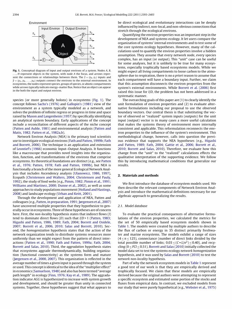
2394 S.R. Borrett, M.A. Freeze / Ecological M
Environment
Object
Input Environ Output Environ
B
C
D
E F
A
B
C
D
G
H
zB
zE
z1
yB
yC
yD
yH
yG
yA
Fig. 1. Conceptual diagram of input and output environs of a system. Nodes A, B,. . ., H represent objects in the system, with node A the focus, and arrows repre-sent the connections or relationships between them. The �z = {zB, zE} inputs and�y = {yA, yB, . . . , yH } outputs connect the environs to the external environment. Inewi
scesrai(M
uaolteefyE1Wa2
chehtH2onuaBtt(aoiptas
cosystems, the nodes represent species, groups of species, or abiotic compartmentshile arrows typically indicate energy–matter flux. Notice that an object can appear
n the both the input and output environ.
pecies (or more generally holons) in ecosystems (Fig. 1). Theoncept follows Sachs’s (1976) and Gallopin’s (1981) view of thenvironment as a system typically modeled as a network, andolves the problem of infinite regress or progress in time and spaceaised by Mason and Langenheim (1957) by specifically identifyingn analytical system boundary. Early applications of the conceptnclude a reconciliation of different aspects of the niche conceptPatten and Auble, 1981) and environmental analysis (Patten and
atis, 1982; Patten et al., 1982a,b).Network Environ Analysis (NEA) is the primary tool scientists
se to investigate ecological environs (Fath and Patten, 1999b; Fathnd Borrett, 2006). The technique is an application and extensionf Leontief’s (1966) economic Input–Output Analysis. It functionsike a macroscope that provides novel insights into the organiza-ion, function, and transformations of the environs that comprisecosystems. Its theoretical foundations are distinct (e.g., see Pattent al., 1976; Patten, 1978; Fath and Patten, 1999b), but NEA isunctionally a branch of the more general Ecological Network Anal-sis that includes Ascendency analysis (Ulanowicz, 1986, 1997),copath (Christensen and Walters, 2004; Christensen and Pauly,992), the study of food webs (e.g., Pimm, 1982; Pimm et al., 1991;illiams and Martinez, 2000; Dunne et al., 2002), as well as some
pproaches to study populations movement (Holland and Hastings,008) and landscape ecology (Urban and Keitt, 2001).
Through the development and application of NEA, Patten andolleagues (e.g., Patten, in preparation, 1991; Jørgensen et al., 2007)ave uncovered multiple properties that they hypothesize to gen-rally occur in ecosystems. Three of these hypotheses are of concernere. First, the non-locality hypothesis states that indirect flows (I)end to dominate direct flows (D) such that I/D > 1 (Patten, 1983;igashi and Patten, 1986, 1989; Fath, 2004; Borrett and Osidele,007; Borrett et al., 2006, 2010; Salas and Borrett, 2010). Sec-nd, the homogenization hypothesis states that the action of theetwork organization tends to distribute systems resources moreniformly than we might expect from the pattern of direct inter-ctions (Patten et al., 1990; Fath and Patten, 1999a; Fath, 2004;orrett and Salas, 2010). Third, the aggradation hypothesis stateshat ecosystems aggrade thermodynamically, building organiza-ion (functional connectivity) as the systems form and matureJørgensen et al., 2000, 2007). This organization is reflected in theverage number of times a given input is passed through the systemr used. This concept is identical to the idea of the “multiplier effect”n economics (Samuelson, 1948) and also has been termed “average
ath length” in ecology (Finn, 1976; Kay et al., 1989). The aggrada-ion indicator AGG is hypothesized to increase with system growthnd development, and should be greater than unity in connectedystems. Together, these hypotheses suggest that what appears toodelling 222 (2011) 2393– 2403
be direct ecological and evolutionary interactions can be deeplyinfluenced by indirect, non-local, and non-obvious connections thatstretch through the ecological environs.
Quantifying the environ properties was an important step in thedevelopment of NEA and systems ecology. It let users compare theorganization of systems’ internal environments and to test some ofthe core systems ecology hypotheses. However, many of the cal-culations used to quantify the environ properties involve a hiddenassumption. They assume that every network node, every speciescomplex, has an input (or output). This “unit” case can be usefulfor some analyses, but it is unlikely to be true for many ecosys-tems, especially trophically based ecosystems models. While wemight expect all living compartments to loose carbon to the atmo-sphere due to respiration, there is no a priori reason to assume thateach compartment will have a boundary input. Further, we claimthat this assumption disconnects the environ properties from thesystem’s external environments. While Borrett et al. (2006) firstraised this issue for I/D, the problem has not been addressed in asystematic manner.
The overarching goals of this paper are (1) to clearly identify theunit formulation of environ properties and (2) to evaluate alter-native formulations including our proposal to use the observedboundary vectors. Our central thesis is that substituting the vec-tor of observed or “realized” system inputs (outputs) for the unitinput (output) vector is in many cases a more useful calculationthat makes the systems theory of environment more internallyconsistent and applicable. This reformulation reconnects the env-iron properties to the influence of the system’s environment. Thismethodological change, however, calls into question the previ-ous evidence that supports the NEA hypotheses (e.g., Higashiand Patten, 1989; Fath, 2004; Gattie et al., 2006; Borrett et al.,2010; Borrett and Salas, 2010). Therefore, we evaluate how thischange from the “unit” to the “realized” calculations effects thequalitative interpretation of the supporting evidence. We followthis by introducing mathematical conditions that generalize ourresults.
2. Materials and methods
We first introduce the database of ecosystem models used. Wethen describe the relevant components of Network Environ Anal-ysis and introduce the mathematical definitions necessary for ouralgebraic approach to generalizing the results.
2.1. Model database
To evaluate the practical consequences of alternative formu-lations of the environ properties, we calculated the metrics forthe set of 50 empirically based ecosystem models shown inTable 1. The models were created by multiple authors to describethe flux of carbon or energy in 35 distinct primarily freshwa-ter and marine ecosystems. The models exhibit a range of sizes(4 ≤ n ≤ 125), connectance (number of direct links divided by thetotal possible number of links; 0.03 ≤ (C = L/n2) ≤ 0.40), and recy-cling (0 ≤ FCI ≤ 0.51). Borrett and Salas (2010) initially collected themodel data set to test the systems ecology network homogenizationhypothesis, and it was used by Salas and Borrett (2010) to test thenetwork non-locality hypothesis.
Part of why the network ecosystem models in Table 1 representa good test of our work is that they are empirically derived andtrophically focused. We claim that these models are empirically
derived because the original authors were attempting to representa specific ecosystem and estimated some portion of the stocks andfluxes from empirical data. In contrast, we excluded models fromour study that were purely hypothetical (e.g., Webster et al., 1975)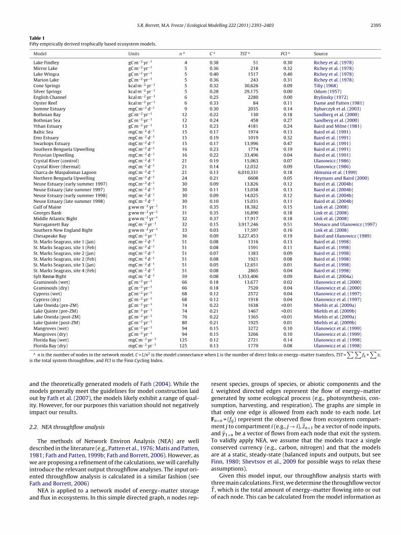
S.R. Borrett, M.A. Freeze / Ecological Modelling 222 (2011) 2393– 2403 2395
Table 1Fifty empirically derived trophically based ecosystem models.
Model Units n a C a TST a FCI a Source
Lake Findley gC m−2 yr−1 4 0.38 51 0.30 Richey et al. (1978)Mirror Lake gC m−2 yr−1 5 0.36 218 0.32 Richey et al. (1978)Lake Wingra gC m−2 yr−1 5 0.40 1517 0.40 Richey et al. (1978)Marion Lake gC m−2 yr−1 5 0.36 243 0.31 Richey et al. (1978)Cone Springs kcal m−2 yr−1 5 0.32 30,626 0.09 Tilly (1968)Silver Springs kcal m−2 yr−1 5 0.28 29,175 0.00 Odum (1957)English Channel kcal m−2 yr−1 6 0.25 2280 0.00 Brylinsky (1972)Oyster Reef kcal m−2 yr−1 6 0.33 84 0.11 Dame and Patten (1981)Somme Estuary mgC m−2 d−1 9 0.30 2035 0.14 Rybarczyk et al. (2003)Bothnian Bay gC m−2 yr−1 12 0.22 130 0.18 Sandberg et al. (2000)Bothnian Sea gC m−2 yr−1 12 0.24 458 0.27 Sandberg et al. (2000)Ythan Estuary gC m−2 yr−1 13 0.23 4181 0.24 Baird and Milne (1981)Baltic Sea mgC m−2 d−1 15 0.17 1974 0.13 Baird et al. (1991)Ems Estuary mgC m−2 d−1 15 0.19 1019 0.32 Baird et al. (1991)Swarkops Estuary mgC m−2 d−1 15 0.17 13,996 0.47 Baird et al. (1991)Southern Benguela Upwelling mgC m−2 d−1 16 0.23 1774 0.19 Baird et al. (1991)Peruvian Upwelling mgC m−2 d−1 16 0.22 33,496 0.04 Baird et al. (1991)Crystal River (control) mgC m−2 d−1 21 0.19 15,063 0.07 Ulanowicz (1986)Crystal River (thermal) mgC m−2 d−1 21 0.14 12,032 0.09 Ulanowicz (1986)Charca de Maspalomas Lagoon mgC m−2 d−1 21 0.13 6,010,331 0.18 Almunia et al. (1999)Northern Benguela Upwelling mgC m−2 d−1 24 0.21 6608 0.05 Heymans and Baird (2000)Neuse Estuary (early summer 1997) mgC m−2 d−1 30 0.09 13,826 0.12 Baird et al. (2004b)Neuse Estuary (late summer 1997) mgC m−2 d−1 30 0.11 13,038 0.13 Baird et al. (2004b)Neuse Estuary (early summer 1998) mgC m−2 d−1 30 0.09 14,025 0.12 Baird et al. (2004b)Neuse Estuary (late summer 1998) mgC m−2 d−1 30 0.10 15,031 0.11 Baird et al. (2004b)Gulf of Maine g ww m−2 yr−1 31 0.35 18,382 0.15 Link et al. (2008)Georges Bank g ww m−2 yr−1 31 0.35 16,890 0.18 Link et al. (2008)Middle Atlantic Bight g ww m−2 yr−1 32 0.37 17,917 0.18 Link et al. (2008)Narragansett Bay mgC m−2 yr−1 32 0.15 3,917,246 0.51 Monaco and Ulanowicz (1997)Southern New England Bight g ww m−2 yr−1 33 0.03 17,597 0.16 Link et al. (2008)Chesapeake Bay mgC m−2 yr−1 36 0.09 3,227,453 0.19 Baird and Ulanowicz (1989)St. Marks Seagrass, site 1 (Jan) mgC m−2 d−1 51 0.08 1316 0.13 Baird et al. (1998)St. Marks Seagrass, site 1 (Feb) mgC m−2 d−1 51 0.08 1591 0.11 Baird et al. (1998)St. Marks Seagrass, site 2 (Jan) mgC m−2 d−1 51 0.07 1383 0.09 Baird et al. (1998)St. Marks Seagrass, site 2 (Feb) mgC m−2 d−1 51 0.08 1921 0.08 Baird et al. (1998)St. Marks Seagrass, site 3 (Jan) mgC m−2 d−1 51 0.05 12,651 0.01 Baird et al. (1998)St. Marks Seagrass, site 4 (Feb) mgC m−2 d−1 51 0.08 2865 0.04 Baird et al. (1998)Sylt Rømø Bight mgC m−2 d−1 59 0.08 1,353,406 0.09 Baird et al. (2004a)Graminoids (wet) gC m−2 yr−1 66 0.18 13,677 0.02 Ulanowicz et al. (2000)Graminoids (dry) gC m−2 yr−1 66 0.18 7520 0.04 Ulanowicz et al. (2000)Cypress (wet) gC m−2 yr−1 68 0.12 2572 0.04 Ulanowicz et al. (1997)Cypress (dry) gC m−2 yr−1 68 0.12 1918 0.04 Ulanowicz et al. (1997)Lake Oneida (pre-ZM) gC m−2 yr−1 74 0.22 1638 <0.01 Miehls et al. (2009a)Lake Quinte (pre-ZM) gC m−2 yr−1 74 0.21 1467 <0.01 Miehls et al. (2009b)Lake Oneida (post-ZM) gC m−2 yr−1 76 0.22 1365 <0.01 Miehls et al. (2009a)Lake Quinte (post-ZM) gC m−2 yr−1 80 0.21 1925 0.01 Miehls et al. (2009b)Mangroves (wet) gC m−2 yr−1 94 0.15 3272 0.10 Ulanowicz et al. (1999)Mangroves (dry) gC m−2 yr−1 94 0.15 3266 0.10 Ulanowicz et al. (1999)Florida Bay (wet) mgC m−2 yr−1 125 0.12 2721 0.14 Ulanowicz et al. (1998)Florida Bay (dry) mgC m−2 yr−1 125 0.13 1779 0.08 Ulanowicz et al. (1998)
a 2 e whe∑∑ ∑
i
amoii
2
d1wieF
a
n is the number of nodes in the network model, C = L/n is the model connectancs the total system throughflow, and FCI is the Finn Cycling Index.
nd the theoretically generated models of Fath (2004). While theodels generally meet the guidelines for model construction laid
ut by Fath et al. (2007), the models likely exhibit a range of qual-ty. However, for our purposes this variation should not negativelympact our results.
.2. NEA throughflow analysis
The methods of Network Environ Analysis (NEA) are wellescribed in the literature (e.g., Patten et al., 1976; Matis and Patten,981; Fath and Patten, 1999b; Fath and Borrett, 2006). However, ase are proposing a refinement of the calculations, we will carefully
ntroduce the relevant output throughflow analyses. The input ori-
nted throughflow analysis is calculated in a similar fashion (seeath and Borrett, 2006)NEA is applied to a network model of energy–matter storagend flux in ecosystems. In this simple directed graph, n nodes rep-
n L is the number of direct links or energy–matter transfers, TST = fij + zi
resent species, groups of species, or abiotic components and theL weighted directed edges represent the flow of energy–mattergenerated by some ecological process (e.g., photosynthesis, con-sumption, harvesting, and respiration). The graphs are simple inthat only one edge is allowed from each node to each node. LetFn×n = (fij) represent the observed flow from ecosystem compart-ment j to compartment i (e.g., j → i), �zn×1 be a vector of node inputs,and �y1×n be a vector of flows from each node that exit the system.To validly apply NEA, we assume that the models trace a singleconserved currency (e.g., carbon, nitrogen) and that the modelsare at a static, steady-state (balanced inputs and outputs, but seeFinn, 1980; Shevtsov et al., 2009 for possible ways to relax theseassumptions).
Given this model input, our throughflow analysis starts withthree main calculations. First, we determine the throughflow vector�T , which is the total amount of energy–matter flowing into or outof each node. This can be calculated from the model information as
2396 S.R. Borrett, M.A. Freeze / Ecological M
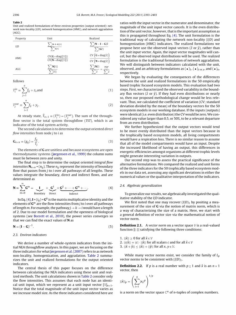
Table 2Unit and realized formulations of three environ properties (output oriented): net-work non-locality (I/D), network homogenization (HMG), and network aggradation(AGG).
Property Unit Realized
I/D
∑(N−I−G)[1]∑
G[1]
∑(N − I − G)�z∑
(G�z)
HMGCV(G ∗ diag([1]))CV(N ∗ diag([1]))
CV(
G ∗ diag(�z))
CV(
N ∗ diag(�z))
f
T
T
fli
fl
G
tm
iflvd
N
eoost
N
2
ttnri
bitcNw
AGG
∑N[1]∑[1]
∑(N�z)∑
�z= TST∑
�z
ollows
ini ≡
n∑j=1
fij + zi,and (1)
outj ≡
n∑i=1
fij + yj. (2)
At steady state, �Tn×1 ≡ (Tini
) = (Toutj
). The sum of the through-ow vector is the total system throughflow (TST), which is an
ndicator of the total system activity.The second calculation is to determine the output oriented direct
ow intensities from node j to i as
n×n ≡ (gij) = fijTj
. (3)
The elements of G are unitless and because ecosystems are openhermodynamic systems (Jørgensen et al., 1999) the column sums
ust lie between zero and unity.The final step is to determine the output oriented integral flow
ntensities Nn×n = (nij). These nij represent the intensity of boundaryow that passes from j to i over all pathways of all lengths. Thesealues integrate the boundary, direct and indirect flows, and areetermined as
≡∞∑
m=0
Gm = I︸︷︷︸Boundary
+ G1︸︷︷︸Direct
+ G2 + · · · + Gm + · · ·︸ ︷︷ ︸Indirect
. (4)
In Eq. (4), I = (iij) = G0 is the matrix multiplicative identity and thelements of Gm are the flow intensities from j to i over all pathwaysf length m. For example, the pathway j → k → i would have a lengthf 2. Due to our model formulation and the openness of biologicalystems (see Borrett et al., 2010), the power series converges sohat we can find the exact values of N as
= (I − G)−1. (5)
.3. Environ indicators
We derive a number of whole-system indicators from the ini-ial NEA throughflow analyses. In this paper, we are focusing on thehree indicators for what Jørgensen et al. (2007) refers to as networkon-locality, homogenization, and aggradation. Table 2 summa-izes the unit and realized formulations for the output orientedndicators.
The central thesis of this paper focuses on the differenceetween calculating the NEA indicators using these unit and real-
zed methods. The unit calculations shown in Table 2 consider only
he flow intensities. This assumes that each node has an identi-al unit input, which we represent as a unit input vector [1]n×1.otice that the total magnitude of the unit input vector varies ase increase model size. As the three indicators considered here areodelling 222 (2011) 2393– 2403
ratios with the input vector in the numerator and denominator, themagnitude of the unit input vector cancels. It is the even distribu-tion of the unit vector, however, that is the important assumption asthis is propagated throughout Eq. (4). The unit formulation is thetraditional way of calculating the network non-locality (I/D) andhomogenization (HMG) indicators. The realized formulations wepropose here use the observed input vectors (�z or �y), rather thanthe unit input vector. Again, the input vector magnitudes will can-cel, but the observed input distributions will be used. The realizedformulation is the traditional formulation of network aggradation.We will distinguish between indicators calculated with the unit,observed, and an arbitrary formulations as ( • )1, ( • )z or y, and ( • )u,respectively.
We began by evaluating the consequences of the differencesbetween the unit and realized formulations in the 50 empiricallybased trophic focused ecosystem models. This evaluation had twosteps. First, we characterized the observed variability in the bound-ary flux vectors (�z or �y). If they had even distributions or nearlyso, then our proposed methodological change would be less rele-vant. Thus, we calculated the coefficient of variation (CV; standarddeviation divided by the mean) of the boundary vectors for the 50ecosystem models in our working database. If the inputs (outputs)were identical (i.e. even distribution) the CV would be zero. We con-sidered any value larger than 0.5, or 50%, to be a relevant departurefrom an even distribution.
We further hypothesized that the output vectors would tendto be more evenly distributed than the input vectors because inthe trophically based ecosystem models, all living compartmentswould have a respiration loss. There is no similar reason to assumethat all of the model compartments would have an input. Despitethe increased likelihood of having an output, this differences inenergetic efficiencies amongst organisms at different trophic levelsmight generate interesting variation in outputs.
Our second step was to assess the practical significance of thealternative formulations. We compared the realized and unit formsof the three indicators for the 50 trophically based ecosystem mod-els in our data set, assessing any significant deviations in either thenumerical values or the qualitative interpretation of the indicators.
2.4. Algebraic generalization
To generalize our results, we algebraically investigated the qual-itative stability of the I/D indicator.
We first noted that one may recover (I/D)1 by positing a mea-surement of the size of G via the notion of matrix norm, which isa way of characterizing the size of a matrix. Here, we start witha general definition of vector size via the mathematical notion ofvector norm.
Definition 2.1. A vector norm on a vector space V is a real-valuedfunction ||· | | satisfying the following three conditions:
1. ||�x|| ≥ 0 for all �x ∈ V2. ||c�x|| = |c| · ||�x|| for all scalars c and for all �x ∈ V3. ||�x + �y|| ≤ ||�x|| + ||�y|| for all x, y ∈ V.
While many vector norms exist, we consider the family of Lp
vector norms to be consistent with (I/D)1.
Definition 2.2. If p is a real number with p ≥ 1 and �x is an n × 1vector, then(
n∑ )1/p
||�x||p =i=1
|xi|p
is a norm on the vector space Cn of n-tuples of complex numbers.
S.R. Borrett, M.A. Freeze / Ecological Modelling 222 (2011) 2393– 2403 2397
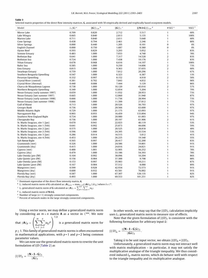
Table 3Selected matrix properties of the direct flow intensity matrices, G, associated with 50 empirically derived and trophically based ecosystem models.
Model �1(G) a ||G | | 1,inb ||G | | 1
c ||(N-I-G) | | 1,ind # SCC e %SCC f
Mirror Lake 0.709 0.820 2.712 5.517 1 60%Lake Wingra 0.665 0.840 2.813 5.135 1 100%Marion Lake 0.711 0.840 2.611 5.640 1 60%Cone Springs 0.438 0.794 2.461 2.246 1 80%Silver Springs 0.000 0.440 1.205 0.101 0 0%English Channel 0.000 0.750 1.687 0.380 0 0%Oyster Reef 0.593 0.829 3.293 5.052 1 83%Somme Estuary 0.483 1.000 7.033 4.740 1 78%Bothnian Bay 0.641 1.000 7.317 14.528 2 83%Bothnian Sea 0.724 1.000 7.438 19.176 2 83%Ythan Estuary 0.678 0.968 6.616 14.197 1 100%Baltic Sea 0.585 1.000 9.250 14.606 2 73%Ems Estuary 0.815 1.000 9.363 37.655 2 60%Swarkops Estuary 0.759 1.000 7.812 20.296 1 67%Southern Benguela Upwelling 0.547 1.000 6.323 6.387 1 13%Peruvian Upwelling 0.332 0.997 8.152 4.918 2 50%Crystal River (control) 0.381 0.702 7.843 4.832 1 90%Crystal River (thermal) 0.440 0.688 7.444 5.129 1 86%Charca de Maspalomas Lagoon 0.738 1.000 16.120 43.016 2 57%Northern Benguela Upwelling 0.349 1.000 12.854 5.204 1 79%Neuse Estuary (early summer 1997) 0.659 1.000 11.932 28.953 1 73%Neuse Estuary (late summer 1997) 0.665 1.000 12.860 31.940 1 87%Neuse Estuary (early summer 1998) 0.666 1.000 11.736 28.994 1 73%Neuse Estuary (late summer 1998) 0.666 1.000 11.399 27.812 1 77%Gulf of Maine 0.713 1.000 20.526 56.793 1 97%Georges Bank 0.736 1.000 20.566 63.600 1 97%Middle Atlantic Bight 0.729 1.000 21.175 63.093 1 97%Narragansett Bay 0.903 0.955 16.459 133.894 1 94%Southern New England Bight 0.724 1.000 20.980 61.003 1 97%Chesapeake Bay 0.736 1.000 20.197 61.906 2 61%St. Marks Seagrass, site 1 (Jan) 0.670 0.941 22.023 46.119 1 53%St. Marks Seagrass, site 1 (Feb) 0.641 0.992 25.873 44.696 1 59%St. Marks Seagrass, site 2 (Jan) 0.575 1.000 20.525 28.818 1 49%St. Marks Seagrass, site 2 (Feb) 0.596 1.000 24.395 33.534 1 53%St. Marks Seagrass, site 3 (Jan) 0.286 0.914 16.515 5.812 1 41%St. Marks Seagrass, site 4 (Feb) 0.453 1.000 26.225 19.340 1 55%Sylt Rømø Bight 0.565 0.997 28.417 32.200 1 83%Graminoids (wet) 0.326 1.000 24.586 19.801 1 91%Graminoids (dry) 0.415 1.000 24.816 24.821 1 91%Cypress (wet) 0.488 1.001 32.905 56.252 1 78%Cypress (dry) 0.479 1.000 33.186 54.393 1 78%Lake Oneida (pre-ZM) 0.164 0.992 38.096 10.204 1 86%Lake Quinte (pre-ZM) 0.156 0.984 37.300 9.798 1 88%Lake Oneida (post-ZM) 0.153 0.997 35.983 10.211 1 87%Lake Quinte (post-ZM) 0.167 0.984 37.512 8.088 1 89%Mangroves (wet) 0.599 0.928 42.934 72.573 1 91%Mangroves (dry) 0.600 0.932 43.581 76.002 1 91%Florida Bay (wet) 0.587 1.000 67.307 128.135 1 82%Florida Bay (dry) 0.493 1.000 69.553 101.251 1 82%
a Dominant eigenvalue of the direct flow intensity matrix, G.b L1 induced matrix norm of G calculated as ||A||p,in = max�x /= 0(||A�x||p/||�x||p) where �x ∈ C
n .c L1 generalized matrix norm of G calculated as ||A||1 =
∑m
i=1
∑n
j=1|aij |.
d L1 induced matrix norm of N-I-G.e
b
t
pip
f
(
Number of large (n > 1) strongly connected components.f Percent of network nodes in the large strongly connected components.
Using a vector norm, we may define a generalized matrix normy considering an m × n matrix A as a vector in C
mn. We note
hat ||A||p =
⎛⎝ m∑
i=1
n∑j=1
|aij|p⎞⎠1/p
is a generalized matrix norm for
≥ 1. This family of generalized matrix norms is often encounteredn mathematical applications, with p = 1 and p = 2 being commonarameter values.
We can now use the generalized matrix norm to rewrite the unit
ormulation of I/D (Table 2) asI/D)1 = ||N - I - G||1||G||1
.
In other words, we may say that the (I/D)1 calculation implicitlyuses L1 generalized matrix norm to measure size of effects.
Note that the given formulation of (I/D)1 is consistent with thefollowing formulation for arbitrary input �u:
(I/D)u = ||(N - I - G)�u||1||G�u||1
.
Taking �u to be unit input vector, we obtain (I/D)u = (I/D)1.Unfortunately, a generalized matrix norm may not interact well
with matrix multiplication – in particular, it may not satisfy themultiplicative analogue of the triangle inequality. We thus consid-ered induced Lp matrix norms, which do behave well with respectto the triangle inequality and its multiplicative analogue.
2 ical M
Di
|
w
pS
G
N
|
|
ts
3
3
at6eLarttW(eti
t(pi�riPS
398 S.R. Borrett, M.A. Freeze / Ecolog
efinition 2.3. Given the vector norm ||x | | p with p ≥ 1, thenduced Lp matrix norm for the matrix A is defined by
|A||p,in = max�x /= 0||As�x||p||�x||p
here �x ∈ Cn.
We illustrate that varying the matrix norm does vary the com-uted value of (I/D)1 by considering computations for the Conepring model, which has the following direct flow intensity matrix.
=
⎡⎢⎢⎣
0 0 0 0 00 0 0 0 0.45330 0.0144 0 0 0.20110 0 0.1552 0 0
0.7941 0.3074 0.0839 0.4514 0
⎤⎥⎥⎦
For this model, the indirect flow intensities are
- I - G =
⎡⎢⎢⎣
0 0 0 0 00.434 0.169 0.084 0.246 0.0930.198 0.077 0.038 0.113 0.0490.030 0.014 0.005 0.017 0.0380.164 0.066 0.101 0.093 0.206
⎤⎥⎥⎦
Using the generalized norm, we find ||N-I-G | | 1 = 2.246 and|G | | 1 = 2.460. Hence (I/D)1 has value
||N-I-G||1||G||1
= 2.2462.460
= 0.913.
Considering induced norm, we have ||N-I-G | | 1,in = 0.828 and|G | | 1,in = 0.794. Hence the corresponding (I/D)1 value is
||N-I-G||1,in
||G||1,in= 0.828
0.794= 1.04.
Clearly the choice of norm used to characterize the size ofhe matrix can influence the indicator outcome. (See Table 3 forelected matrix properties of G).
. Results
.1. Boundary variability
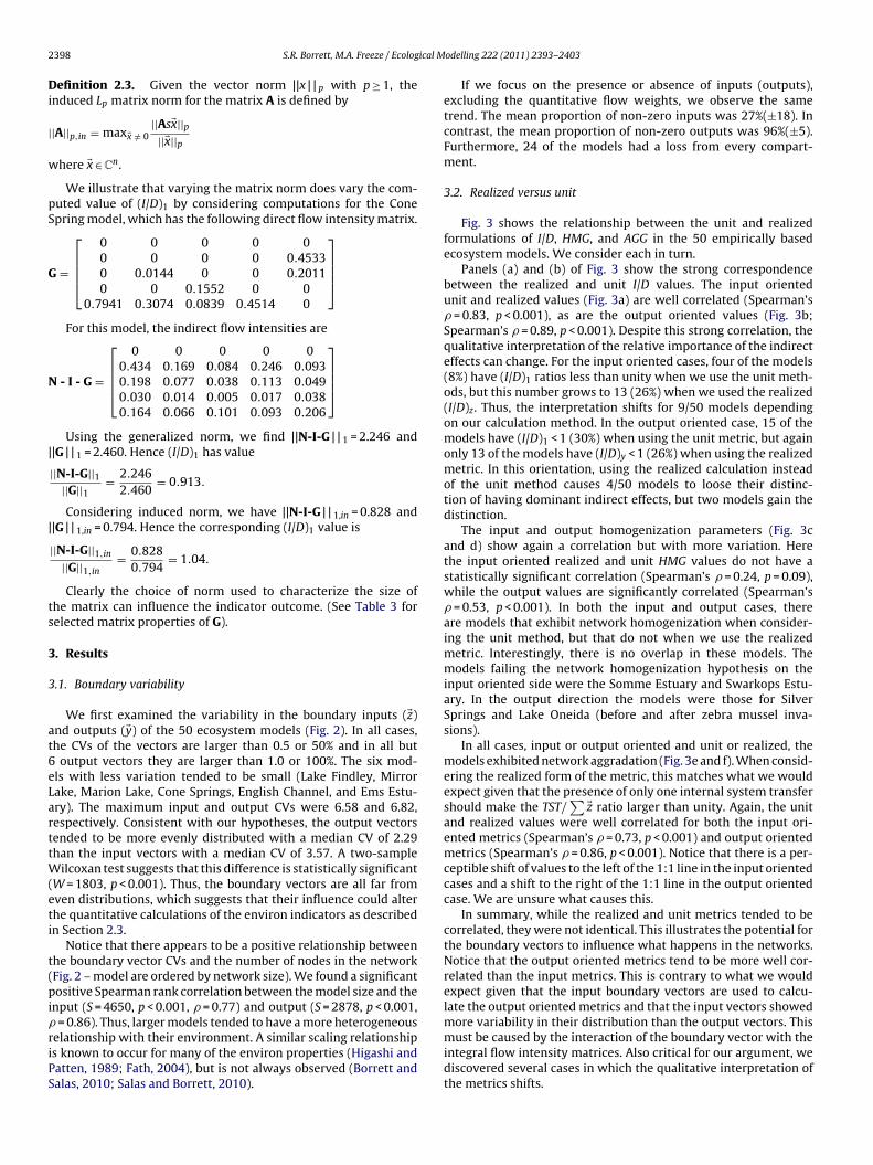
We first examined the variability in the boundary inputs (�z)nd outputs (�y) of the 50 ecosystem models (Fig. 2). In all cases,he CVs of the vectors are larger than 0.5 or 50% and in all but
output vectors they are larger than 1.0 or 100%. The six mod-ls with less variation tended to be small (Lake Findley, Mirrorake, Marion Lake, Cone Springs, English Channel, and Ems Estu-ry). The maximum input and output CVs were 6.58 and 6.82,espectively. Consistent with our hypotheses, the output vectorsended to be more evenly distributed with a median CV of 2.29han the input vectors with a median CV of 3.57. A two-sample
ilcoxan test suggests that this difference is statistically significantW = 1803, p < 0.001). Thus, the boundary vectors are all far fromven distributions, which suggests that their influence could alterhe quantitative calculations of the environ indicators as describedn Section 2.3.
Notice that there appears to be a positive relationship betweenhe boundary vector CVs and the number of nodes in the networkFig. 2 – model are ordered by network size). We found a significantositive Spearman rank correlation between the model size and the
nput (S = 4650, p < 0.001, � = 0.77) and output (S = 2878, p < 0.001, = 0.86). Thus, larger models tended to have a more heterogeneous
elationship with their environment. A similar scaling relationships known to occur for many of the environ properties (Higashi andatten, 1989; Fath, 2004), but is not always observed (Borrett andalas, 2010; Salas and Borrett, 2010).odelling 222 (2011) 2393– 2403
If we focus on the presence or absence of inputs (outputs),excluding the quantitative flow weights, we observe the sametrend. The mean proportion of non-zero inputs was 27%(±18). Incontrast, the mean proportion of non-zero outputs was 96%(±5).Furthermore, 24 of the models had a loss from every compart-ment.
3.2. Realized versus unit
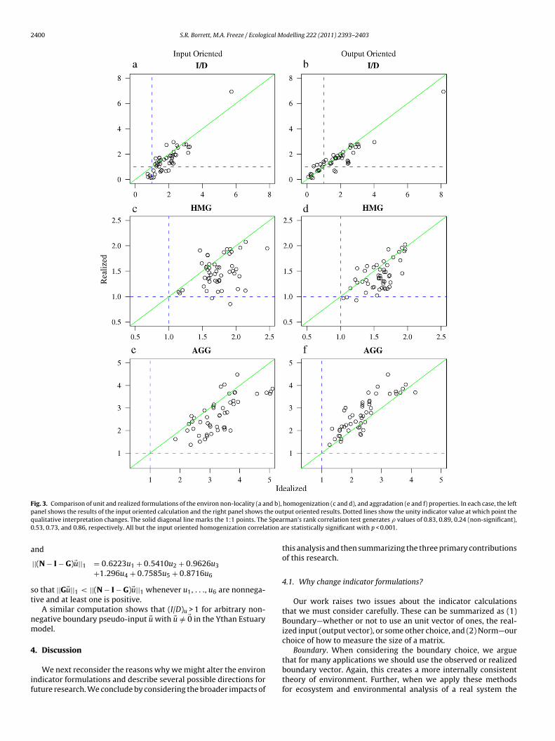
Fig. 3 shows the relationship between the unit and realizedformulations of I/D, HMG, and AGG in the 50 empirically basedecosystem models. We consider each in turn.
Panels (a) and (b) of Fig. 3 show the strong correspondencebetween the realized and unit I/D values. The input orientedunit and realized values (Fig. 3a) are well correlated (Spearman’s� = 0.83, p < 0.001), as are the output oriented values (Fig. 3b;Spearman’s � = 0.89, p < 0.001). Despite this strong correlation, thequalitative interpretation of the relative importance of the indirecteffects can change. For the input oriented cases, four of the models(8%) have (I/D)1 ratios less than unity when we use the unit meth-ods, but this number grows to 13 (26%) when we used the realized(I/D)z. Thus, the interpretation shifts for 9/50 models dependingon our calculation method. In the output oriented case, 15 of themodels have (I/D)1 < 1 (30%) when using the unit metric, but againonly 13 of the models have (I/D)y < 1 (26%) when using the realizedmetric. In this orientation, using the realized calculation insteadof the unit method causes 4/50 models to loose their distinc-tion of having dominant indirect effects, but two models gain thedistinction.
The input and output homogenization parameters (Fig. 3cand d) show again a correlation but with more variation. Herethe input oriented realized and unit HMG values do not have astatistically significant correlation (Spearman’s � = 0.24, p = 0.09),while the output values are significantly correlated (Spearman’s� = 0.53, p < 0.001). In both the input and output cases, thereare models that exhibit network homogenization when consider-ing the unit method, but that do not when we use the realizedmetric. Interestingly, there is no overlap in these models. Themodels failing the network homogenization hypothesis on theinput oriented side were the Somme Estuary and Swarkops Estu-ary. In the output direction the models were those for SilverSprings and Lake Oneida (before and after zebra mussel inva-sions).
In all cases, input or output oriented and unit or realized, themodels exhibited network aggradation (Fig. 3e and f). When consid-ering the realized form of the metric, this matches what we wouldexpect given that the presence of only one internal system transfershould make the TST/
∑ �z ratio larger than unity. Again, the unitand realized values were well correlated for both the input ori-ented metrics (Spearman’s � = 0.73, p < 0.001) and output orientedmetrics (Spearman’s � = 0.86, p < 0.001). Notice that there is a per-ceptible shift of values to the left of the 1:1 line in the input orientedcases and a shift to the right of the 1:1 line in the output orientedcase. We are unsure what causes this.
In summary, while the realized and unit metrics tended to becorrelated, they were not identical. This illustrates the potential forthe boundary vectors to influence what happens in the networks.Notice that the output oriented metrics tend to be more well cor-related than the input metrics. This is contrary to what we wouldexpect given that the input boundary vectors are used to calcu-late the output oriented metrics and that the input vectors showedmore variability in their distribution than the output vectors. This
must be caused by the interaction of the boundary vector with theintegral flow intensity matrices. Also critical for our argument, wediscovered several cases in which the qualitative interpretation ofthe metrics shifts.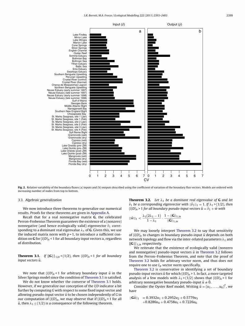
S.R. Borrett, M.A. Freeze / Ecological Modelling 222 (2011) 2393– 2403 2399
Input (z)
0 1 2 3 4 5 6 7
Florida Bay (dry)Florida Bay (wet)Mangroves (dry)Mangroves (wet)
Lake Quinte (post −ZM)Lake Oneida (p ost−ZM)
Lake Quinte (pre−Z M)Lake Oneida (pre−ZM)
Cypress (dry)Cypress (wet)
Graminoids (dry)Graminoids (wet)Sylt Rømø Bight
St. Marks Seagrass, site 4 (Feb)St. Marks Seagrass, site 3 (Jan)St. Marks Seagrass, site 2 (Feb)St. Marks Seagrass, site 2 (Jan)St. Marks Seagrass, site 1 (Feb)St. Marks Seagrass, site 1 (Jan)
Chesapeake BaySouthern New England Bight
Narraganse tt BayMiddle Atlantic Bight
Georges BankGulf of Maine
Neuse Estuary (late summer 1998)Neuse Estuary (early summer 1998)
Neuse Estuary (late summer 1997)Neuse Estuary (early summer 1997)
Northern Benguela Up wellingCharca de Maspalomas Lagoo n
Crystal River (thermal)Crystal River (control)
Peruvian UpwellingSouthern Benguela Up welling
Swarkops Estua ryEms Estuary
Baltic SeaYthan EstuaryBothnian SeaBothnian Bay
Somme EstuaryOyster Reef
English ChannelSilver SpringsCone Springs
Marion LakeLake WingraMirror Lake
Lake Findleya
Output (y)
0 1 2 3 4 5 6 7
b
CV
→ →
F d usini
3
r
Pnstdo
Ti
S
Hfaou
ig. 2. Relative variability of the boundary fluxes (a) inputs and (b) outputs describencreasing number of nodes from top to bottom.
.3. Algebraic generalization
We now introduce three theorems to generalize our numericalesults. Proofs for these theorems are given in Appendix A.
Recall that for a real nonnegative matrix G, the celebratederron-Frobenius Theorem guarantees the existence of a (nonzero)onnegative (and hence ecologically valid) eigenvector �v1 corre-ponding to a dominant real eigenvalue �1 of G. Given this, we usehe induced matrix norm with p = 1, to introduce a sufficient con-ition on G for (I/D)u < 1 for all boundary input vectors u, regardlessf distribution.
heorem 3.1. If ||G | | 1,in < (1/2), then (I/D)u < 1 for all boundarynput vectors �u.
We note that (I/D)u < 1 for arbitrary boundary input �u in theilver Springs model since the condition of Theorem 3.1 is satisfied.
We do not know whether the converse of Theorem 3.1 holds.owever, if we generalize our conception of the I/D indicator a bit
urther by computing G with respect to some fixed input vector andllowing pseudo-input vector �u to be chosen independently of G inur computation of (I/D)u, we may observe that if (I/D)u < 1 for all
� , then �1 ≤ (1/2) is a consequence of the following theorem.
g the coefficient of variation of the boundary flux vectors. Models are ordered with
Theorem 3.2. Let �1 be a dominant real eigenvalue of G and let�v1 be a corresponding eigenvector with ||�v1||1 = 1. If �1 > (1/2), then(I/D)u > 1 for all boundary pseudo-input vectors �u = �v1 + �w with
|| �w||1 <�1(2�1 − 1)
1 − �1· 1 − ||G||1,in
||G||1,in
We may loosely interpret Theorem 3.2 to say that sensitivityof (I/D)u to changes in boundary pseudo-input �u depends on bothnetwork topology and flow via the inter-related parameters �1 and||G | | 1,in respectively.
We reiterate that the existence of ecologically valid (nonzeroand nonnegative) pseudo-input vectors �u in Theorem 3.2 followsfrom the Perron–Frobenius Theorem, and note that the proof ofTheorem 3.2 holds for arbitrary vector norm, and thus does notrequire one to use Lp vector norm specifically.
Theorem 3.2 is conservative in identifying a set of boundarypseudo-input vectors �u for which (I/D)u > 1. In fact, a more targetedanalysis of a few models with �1 > (1/2) shows that (I/D)u > 1 forarbitrary nonnegative boundary pseudo-input �u /= �0.
Consider the Oyster Reef model. Writing �u = (u1, . . . , u6)T , we
have||G�u||1 = 0.3932u1 + 0.2952u2 + 0.5779u3+0.8286u4 + 0.4758u5 + 0.7226u6
2400 S.R. Borrett, M.A. Freeze / Ecological Modelling 222 (2011) 2393– 2403
Fig. 3. Comparison of unit and realized formulations of the environ non-locality (a and b), homogenization (c and d), and aggradation (e and f) properties. In each case, the leftp he ouq Spea0 tion a
a
st
nm
4
if
anel shows the results of the input oriented calculation and the right panel shows tualitative interpretation changes. The solid diagonal line marks the 1:1 points. The.53, 0.73, and 0.86, respectively. All but the input oriented homogenization correla
nd
||(N − I − G)�u||1 = 0.6223u1 + 0.5410u2 + 0.9626u3+1.296u4 + 0.7585u5 + 0.8716u6
o that ||G�u||1 < ||(N − I − G)�u||1 whenever u1, . . ., u6 are nonnega-ive and at least one is positive.
A similar computation shows that (I/D)u > 1 for arbitrary non-egative boundary pseudo-input �u with �u /= �0 in the Ythan Estuaryodel.
. Discussion
We next reconsider the reasons why we might alter the environndicator formulations and describe several possible directions foruture research. We conclude by considering the broader impacts of
tput oriented results. Dotted lines show the unity indicator value at which point therman’s rank correlation test generates � values of 0.83, 0.89, 0.24 (non-significant),re statistically significant with p < 0.001.
this analysis and then summarizing the three primary contributionsof this research.
4.1. Why change indicator formulations?
Our work raises two issues about the indicator calculationsthat we must consider carefully. These can be summarized as (1)Boundary—whether or not to use an unit vector of ones, the real-ized input (output vector), or some other choice, and (2) Norm—ourchoice of how to measure the size of a matrix.
Boundary. When considering the boundary choice, we argue
that for many applications we should use the observed or realizedboundary vector. Again, this creates a more internally consistenttheory of environment. Further, when we apply these methodsfor ecosystem and environmental analysis of a real system the
ical M
bitumlrcBttTit
tosaorua
4
d
cibc
crpiie
Ematctmmtgnifn
4
avqeabt
S.R. Borrett, M.A. Freeze / Ecolog
oundary observations are a critical component to understand-ng the functioning of the real system. This is a similar argumenthat Borrett et al. (2006) made when they first considered andsed what we are calling the realized formulation. However, thereay be occasions when considering alternative boundary vectors
ike the unit input vectors is useful. For example, the originalational for using the unit vector was to facilitate within systemomparison of environs (e.g. Patten and Auble, 1981). Further,orrett et al. (2010) chose to report (I/D)1 specifically becausehey were considering the connections between this network fea-ure, �1(G), and cumulative flow in the path series of Eq. (3).hese connections would have been less obvious had they alsoncorporated the variability introduced by the boundary vec-ors.
Norm. We have seen in Section 2.4 that the qualitative interpre-ation of the computed value of a I/D index varies with the choicef matrix norm, even when boundary input is not explicitly con-idered. Moreover, although the proofs of Theorems 3.1 and 3.2re stated in terms of L1 norm for consistency with considerationf unit and realized I/D elsewhere in the paper, analogous theo-ems continue to hold in Lp norm for p ≥ 1. Thus, the choice of normsed to describe the system and its associated matrices becomesn interesting question.
.2. Future work
The work presented here forms a foundation for at least threeirections for future work.
First, as discussed previously we need to further consider thehoice of mathematical norm we use to construct network analysisndicators. The generalized matrix norm that the community haseen using makes intuitive sense for biological applications, butonsidering other norms may lead to more robust metrics (Table 3).
Second, in this paper we only consider three of the environ indi-ator from Ecological Network Analysis (ENA), but the issues weaise will likely effect other indicators as well. An obvious exam-le is the synergism property (Fath and Patten, 1998), but other
ndicators may benefit from a careful review. Whipple et al. (2007)ndicate how this issue might further effect the formal analysis ofnvirons.
The third direction concerns the mathematical formulation ofNA. Here, we fruitfully dug deeper into the underlying mathe-atics of the analysis and we encourage a continuation of this
pproach. For example, we wonder if network models of ecosys-ems might have a consistent set of characteristics such that theyan be defined as a mathematical subclass of matrices. We couldhen use this model classification to investigate the general mathe-
atical properties of this subclass. Further, we are curious about theathematical similarities and distinctions between these ecosys-
em networks and other types of biological network models (e.g.,ene and protein interaction networks). What is the relevant exter-al environment for a genetic network and how is it incorporated
nto the analysis? We argue that this is an important direction ofuture work for building a robust formal theory of environment andetwork science.
.3. Broader impacts
This study delves into the fine details of ecosystem networknalysis methodology, but the work contributes to a broader con-ersation concerning community and ecosystem interactions anduite possibly cellular systems biology. Network models are gen-
rally useful for representing relationships among parts of ant least partially connected system. Often the models used areinary, simply representing the presence or absence of connec-ions. There is a long history of investigating community foododelling 222 (2011) 2393– 2403 2401
webs with this type of model (e.g. Pimm, 1982; Cohen et al.,1990; Dunne et al., 2002) and a growing literature on mutu-alistic communities (e.g. Jordano et al., 2003; Bascompte andJordano, 2007). The problem is that knowledge of the binarypresence–absence of a connection may be insufficient to under-stand the system function and behavior of interest. We often needto know the strength of interactions. This is not a new concern(Berlow et al., 2004), but our work highlights a new aspect ofit.
In our analysis we have estimates of the internal system strengthof interactions, but through our analytical choices we comparedwhether the boundary flows were all equally present (zi = 1 oryi = 1) or differed quantitatively due to physical and biological con-straints. This work shows how the energy distribution into and thenthrough the networks can strongly effect the effective network con-nectance as reflected in the environ properties we investigated. Thisfurther suggests that quantitative estimates of these strengths ofinteraction (energy–matter flux, evolutionary selection pressure,pollinator visitations, etc.) are essential to understanding the sys-tems organization.
4.4. Summary and conclusions
The work reported in this paper makes three primary con-tributions to the systems ecology literature. First, we expose ahidden assumption in many of the environ property indicator cal-culations and consider alternative formulations. We suggest thatusing the observed boundary vector in these calculations mightbe more appropriate for many applications and we claim thatit makes the theory more internally consistent. We show thatwhile the two methods tend to generate similar results, there arecases in which the qualitative interpretation changes. The secondcontribution is the presentation of the input and output envi-ron properties for the 50 empirically derived models. While someof the metrics have been published previously, they tended tofocus on either the input or output orientation and either usedthe unit or realized formulation. Here, we summarize all of thevalues, which consistently provide support for the systems ecol-ogy hypotheses of non-locality, homogenization, and aggradation.The third contribution is the algebraic generalizations of the env-iron calculation results. Further, we provide new theorems thatdescribe conditions on the eigenvalues of the direct flow intensitymatrix, G, for when the indirect flow intensities will necessarilybe greater or less than the direct flow intensities. This work isa step toward a formal re-evaluation of the NEA calculus and ageneral strengthening of the environ based formal theory of envi-ronment.
Acknowledgements
This contribution benefited from reviews by A.K. Salas, S.L. Fann,A. Stapleton, B.C. Patten, S.J. Whipple, and three anonymous review-ers. We also would like to thank the multiple investigators whogenerously shared their network models with us including D. Baird,R.R. Christian, A.L.J. Miehls, J. Link, R.E. Ulanowicz. UNCW fundedthis work.
Appendix A.
We provide proofs of the theorems stated in the paper.
Theorem. If ||G | | 1,in < (1/2), then (I/D)u < 1 for all boundary inputvectors �u.
2 ical M
Pi
w|
w
Tcf
|
Pta
w|
ac
w
402 S.R. Borrett, M.A. Freeze / Ecolog
roof of Theorem 3.1. Recall that ||· | | 1,in satisfies the trianglenequality and its multiplicative analogue. We thus obtain that
||∞∑
m=1
Gm||1,in ≤∞∑
m=1
||Gm||1,in
≤∞∑
m=1
||G||m1,in,
here the latter sum is a convergent geometric series since|G | | 1,in < (1/2) < 1.
Now observe that
||(N-I-G)�u||1 = ||∞∑
m=2
Gm �u||1
= ||(∞∑
m=1
Gm)G�u||1
≤ ||∞∑
m=1
Gm||1,in · ||G�u||1
≤ ||G||1,in
1 − ||G||1,in· ||G�u||1
< ||G�u||1
henever ||G | | 1,in < (1/2). �
heorem. Let �1 be a dominant real eigenvalue of G and let �v1 be aorresponding eigenvector with ||�v1||1 = 1. If �1 > (1/2), then (I/D)u > 1or all boundary pseudo-input vectors �u = �v1 + �w with
| �w||1 <�1(2�1 − 1)
1 − �1· 1 − ||G||1,in
||G||1,in
roof of Theorem 3.2. As in the proof of Theorem 3.1, we notehat ||· | | 1,in satisfies the triangle inequality and its multiplicativenalogue, and thus obtain that
||∞∑
m=2
Gm||1,in ≤∞∑
m=2
||Gm||1,in
≤∞∑
m=2
||G||m1,in,
here the latter geometric series converges since|G | | 1,in < (1/2) < 1, and has sum (||G||21,in
/(1 − ||G||1,in)).We further note that the Perron–Frobenius Theorem provides
(nonzero) nonnegative (hence ecologically valid) eigenvector �v1orresponding to a dominant real eigenvalue �1 of G.
Now observe that
||(N-I-G)�u||1 = ||∞∑
m=2
Gm �u||1
= || �21
1 − �1�v1 +
∞∑m=2
Gm �w||1
≥ || �21
1 − �1�v1||1 − ||
∞∑m=2
Gm �w||1
≥ �21
1 − �1−
||G||21,in
1 − ||G||1,in· || �w||1
> �1 + ||G||1,in · || �w||1≥ ||G�u||1
henever || �w||1 < (�1(2�1 − 1)/1 − �1) · (1 − ||G||1,in/||G||1,in). �
odelling 222 (2011) 2393– 2403
References
Alley, T.R., 1985. Organism-environment mutuality epistemics, and the concept ofan ecological niche. Synthese 65, 411–444.
Almunia, J., Basterretxea, G., Aistegui, J., Ulanowicz, R.E., 1999. Benthic-pelagicswitching in a coastal subtropical lagoon. Estuar. Coast. Shelf Sci. 49, 221–232.
Baird, D., Asmus, H., Asmus, R., 2004a. Energy flow of a boreal intertidal ecosystem,the Sylt-Rømø Bight. Mar. Ecol. Prog. Ser. 279, 45–61.
Baird, D., Christian, R.R., Peterson, C.H., Johnson, G.A., 2004b. Consequences ofhypoxia on estuarine ecosystem function: energy diversion from consumers tomicrobes. Ecol. Appl. 14, 805–822.
Baird, D., Luczkovich, J., Christian, R.R., 1998. Assessment of spatial and tempo-ral variability in ecosystem attributes of the St Marks national wildlife refuge,Apalachee Bay, Florida. Estuar. Coast. Shelf Sci. 47, 329–349.
Baird, D., McGlade, J.M., Ulanowicz, R.E., 1991. The comparative ecology of six marineecosystems. Philos. Trans. R. Soc. Lond. B 333, 15–29.
Baird, D., Milne, H., 1981. Energy flow in the Ythan Estuary, Aberdeenshire, Scotland.Estuar. Coast. Shelf Sci. 13, 455–472.
Baird, D., Ulanowicz, R.E., 1989. The seasonal dynamics of the Chesapeake Bayecosystem. Ecol. Monogr. 59, 329–364.
Bascompte, J., Jordano, P., 2007. Plant-animal mutualistic networks: the architectureof biodiversity. Ann. Rev. Ecol. Evol. Syst. 38, 567–593.
Berlow, E.L., Neutel, A.M., Cohen, J.E., de Ruiter, P.C., Ebenman, B., Emmerson, M.,Fox, J.W., Jansen, V.A.A., Jones, J.I., Kokkoris, G.D., Logofet, D.O., McKane, A.J.,Montoya, J.M., Petchey, O., 2004. Interaction strengths in food webs: issues andopportunities. J. Anim. Ecol. 73 (3), 585–598.
Borrett, S.R., Osidele, O.O., 2007. Environ indicator sensitivity to flux uncertainty ina phosphorus model of Lake Sidney Lanier, USA. Ecol. Model. 200, 371–383.
Borrett, S.R., Salas, A.K., 2010. Evidence for resource homogenization in 50 trophicecosystem networks. Ecol. Model. 221, 1710–1716.
Borrett, S.R., Whipple, S.J., Patten, B.C., 2010. Rapid development of indirect effectsin ecological networks. Oikos 119, 1136–1148.
Borrett, S.R., Whipple, S.J., Patten, B.C., Christian, R.R., 2006. Indirect effects anddistributed control in ecosystems 3. Temporal variability of indirect effectsin a seven-compartment model of nitrogen flow in the Neuse River Estuary(USA)—time series analysis. Ecol. Model., 178–188.
Bregman, J.I., Mackenthun, K.M., 1992. Environmental Impact Statements. LewisPublishers, Boca Raton.
Brylinsky, M., 1972. Steady-state sensitivity analysis of energy flow in a marineecosystem. In: Patten, B.C. (Ed.), Systems Analysis and Simulation in Ecology,vol. 2. Academic Press, pp. 81–101.
Christensen, V., Pauly, D., 1992. Ecopath-II—a software for balancing steady-stateecosystem models and calculating network characteristics. Ecol. Model. 61,169–185.
Christensen, V., Walters, C.J., 2004. Ecopath with Ecosim: methods, capabilities andlimitations. Ecol. Model. 172, 109–139.
Cohen, J.E., Briand, F., Newman, C.M., 1990. Community Food Webs: Data and Theory.Springer-Verlag, New York.
Dame, R.F., Patten, B.C., 1981. Analysis of energy flows in an intertidal oyster reef.Mar. Ecol. Prog. Ser. 5, 115–124.
Dunne, J.A., Williams, R.J., Martinez, N.D., 2002. Network topology and biodiversityloss in food webs: robustness increases with connectance. Ecol. Lett. 5, 558–567.
Eccleston, C.E., 2001. Effective Environmental Assessments: How to Manage andPrepare NEPA EAs. Lewis Publishers, Boca Raton.
Fath, B.D., 2004. Network analysis applied to large-scale cyber-ecosystems. Ecol.Model. 171, 329–337.
Fath, B.D., Borrett, S.R., 2006. A Matlab©function for network environ analysis. Env-iron. Model. Softw. 21, 375–405.
Fath, B.D., Patten, B.C., 1998. Network synergism: emergence of positive relations inecological systems. Ecol. Model. 107, 127–143.
Fath, B.D., Patten, B.C., 1999a. Quantifying resource homogenization using networkflow analysis. Ecol. Model. 107, 193–205.
Fath, B.D., Patten, B.C., 1999b. Review of the foundations of network environ analysis.Ecosystems 2, 167–179.
Fath, B.D., Scharler, U.M., Ulanowicz, R.E., Hannon, B., 2007. Ecological networkanalysis: network construction. Ecol. Model. 208, 49–55.
Finn, J.T., 1976. Measures of ecosystem structure and function derived from analysisof flows. J. Theor. Biol. 56, 363–380.
Finn, J.T., 1980. Flow analysis of models of the Hubbard Brook ecosystem. Ecology61, 562–571.
Gallopin, G.C., 1981. The abstract concept of environment. Int. J. Gen. Syst. 7,139–149.
Gattie, D.K., Schramski, J.R., Borrett, S.R., Patten, B.C., Bata, S.A., Whipple, S.J., 2006.Indirect effects and distributed control in ecosystems: network environ analysisof a seven-compartment model of nitrogen flow in the Neuse River Estuary,USA—steady-state analysis. Ecol. Model. 194, 162–177.
Haskell, E.F., 1940. Mathematical systematization of “environment”, “organism”, and“habitat”. Ecology 21, 1–16.
Heymans, J.J., Baird, D., 2000. A carbon flow model and network analysis of theNorthern Benguela upwelling system, Namibia. Ecol. Model. 126, 9–32.
Higashi, M., Patten, B.C., 1986. Further aspects of the analysis of indirect effects in
ecosystems. Ecol. Model. 31, 69–77.Higashi, M., Patten, B.C., 1989. Dominance of indirect causality in ecosystems. Am.Nat. 133, 288–302.
Holland, M.D., Hastings, A., 2008. Strong effect of dispersal network structure onecological dynamics. Nature 456, 792–794.

ical M
J
J
J
J
K
K
LL
M
M
M
M
M
O
P
P
P
P
P
P
PP
P
P
S.R. Borrett, M.A. Freeze / Ecolog
ordano, P., Bascompte, J., Olesen, J.M., 2003. Invariant properties in coevolutionarynetworks of plant-animal interactions. Ecol. Lett. 6, 69–81.
ørgensen, S.E., Fath, B.D., Bastianoni, S., Marques, J.C., Müller, F., Nielsen, S., Pat-ten, B.C., Tiezzi, E., Ulanowicz, R.E., 2007. A New Ecology: Systems Perspective.Elsevier, Amsterdam.
ørgensen, S.E., Patten, B.C., Straskraba, M., 1999. Ecosystems emerging. 3. Openness.Ecol. Model. 117, 41–64.
ørgensen, S.E., Patten, B.C., Straskraba, M., 2000. Ecosystems emerging. 4. Growth.Ecol. Model. 126, 249–284.
ates, R.W., Clark, W.C., Corell, R., Hall, J.M., Jaeger, C.C., Lowe, I., McCarthy, J.J.,Schellnhuber, H.J., Bolin, B., Dickson, N., Faucheux, S., Gallopin, G.C., Grubler,A., Huntley, B., Jager, J., Jodha, N.S., Kasperson, R., Mabogunje, A., Matson,P., Mooney, H., Moore, B., O’Riordan, T., Svedin, U., 2001. Environment anddevelopment—sustainability science. Science 292 (5517), 641–642.
ay, J.J., Graham, L.A., Ulanowicz, R.E., 1989. A detailed guide to network analysis.In: Wulff, F., Field, J.G., Mann, K.H. (Eds.), Network Analysis in Marine Ecology:Methods and Applications. Springer-Verlag, Heidelburg, pp. 15–61.
eontief, W.W., 1966. Input–Output Economics. Oxford University Press, New York.ink, J., Overholtz, W., O’Reilly, J., Green, J., Dow, D., Palka, D., Legault, C., Vitaliano,
J., Guida, V., Fogarty, M., Brodziak, J., Methratta, L., Stockhausen, W., Col, L., Gris-wold, C., 2008. The northeast US continental shelf energy modeling and analysisexercise (EMAX): ecological network model development and basic ecosystemmetrics. J. Mar. Syst. 74, 453–474.
ason, H.L., Langenheim, J.H., 1957. Language analysis and the concept environ-ment. Ecology 38, 325–340.
atis, J.H., Patten, B.C., 1981. Environ analysis of linear compartmental systems: thestatic, time invariant case. Bull. Int. Stat. Inst. 48, 527–565.
iehls, A.L.J., Mason, D.M., Frank, K.A., Krause, A.E., Peacor, S.D., Taylor, W.W., 2009a.Invasive species impacts on ecosystem structure and function: a comparison ofOneida Lake, New York, USA, before and after zebra mussel invasion. Ecol. Model.220 (22), 3194–3209.
iehls, A.L.J., Mason, D.M., Frank, K.A., Krause, A.E., Peacor, S.D., Taylor, W.W., 2009b.Invasive species impacts on ecosystem structure and function: a comparison ofthe Bay of Quinte, Canada, and Oneida Lake, USA, before and after zebra musselinvasion. Ecol. Model. 220, 3182–3193.
onaco, M.E., Ulanowicz, R.E., 1997. Comparative ecosystem trophic structure ofthree us mid-Atlantic estuaries. Mar. Ecol. Prog. Ser. 161, 239–254.
dum, H.T., 1957. Trophic structure and productivity of Silver Springs, Florida. Ecol.Monogr. 27, 55–112.
atten, B., 1983. On the quantitative dominance of indirect effects in ecosystems. In:Lauenroth, W.K., Skogerboe, G.V., Flug, M. (Eds.), Analysis of Ecological Systems:State-of-the-art in Ecol Mod. Elsevier, Amsterdam, pp. 27–37.
atten, B., Barber, M.C., Durham, S., 1982a. Synthesis and analysis of data and eco-logical modelling for salt dome brine discharge sites in the Gulf of Mexico,Task III. Final Report. Ecology Simulations, Inc. Submitted to: U.S. Departmentof Commerce, National Oceanic and Atmospheric Administration, Environmen-tal Data and Information Service, Center for Environmental Assessment Service.Submitted by: Ecology Simulations, Inc., Athens, GA.
atten, B., Higashi, M., Burns, T., 1990. Trophic dynamics in ecosystem networks:significance of cycles and storage. Ecol. Model. 51, 1–28.
atten, B., Matis, J., 1982. The water environs of the Okefenokee Swamp: an appli-cation of static linear environ analysis. Ecol. Model. 16, 1–50.
atten, B., Richardson, T., Barber, M., 1982b. Path analysis of a reservoir ecosystemmodel. Can. Water Res. J. 7, 252–282.
atten, B.C., 1978. Systems approach to the concept of environment. Ohio J. Sci. 78,206–222.
atten, B.C., 1981. Environs: the superniches of ecosystems. Am. Zool. 21, 845–852.atten, B.C., 1982. Environs: relativistic elementary particles for ecology. Am. Nat.
119, 179–219.atten, B.C., 1991. Network ecology: indirect determination of the life-environment
relationship in ecosystems. In: Higashi, M., Burns, T. (Eds.), Theoretical Studies ofEcosystems: The Network Perspective. Cambridge University Press, New York,pp. 288–351.
atten, B.C., 2001. Jakob von Uexkull and the theory of environs. Semiotica 134,423–443.
odelling 222 (2011) 2393– 2403 2403
Patten, B.C., in preparation. Holoecology: The Unification of Nature by NetworkIndirect Effects. Columbia University Press, New York.
Patten, B.C., Auble, G.T., 1981. System theory of the ecological niche. Am. Nat. 117,893–922.
Patten, B.C., Bosserman, R.W., Finn, J.T., Cale, W.G., 1976. Propagation of cause inecosystems. In: Patten, B.C. (Ed.), Systems Analysis and Simulation in Ecology,vol. IV. Academic Press, New York, pp. 457–579.
Pimm, S.L., 1982. Food Webs. Chapman and Hall, London, New York.Pimm, S.L., Lawton, J.H., Cohen, J.E., 1991. Food web patterns and their consequences.
Nature 350 (6320), 669–674.Richey, J.E., Wissmar, R.C., Devol, A.H., Likens, G.E., Eaton, J.S., Wetzel, R.G., Odum,
W.E., Johnson, N.M., Loucks, O.L., Prentki, R.T., Rich, P.H., 1978. Carbon flow infour lake ecosystems: a structural approach. Science 202, 1183–1186.
Rybarczyk, H., Elkaim, B., Ochs, L., Loquet, N., 2003. Analysis of the trophic networkof a macrotidal ecosystem: the Bay of Somme (eastern channel). Estuar. Coast.Shelf Sci. 58, 405–421.
Sachs, W.M., 1976. Toward formal foundations of teleological systems science. Gen.Syst. 21, 145–153.
Salas, A.K., Borrett, S.R., 2010. Evidence for dominance of indirect effects in ecosys-tem networks. arXiv:10091841 [q-bio].
Samuelson, P.A., 1948. Economics: An Introductory Analysis. McGraw-Hill Book Co.,New York.
Sandberg, J., Elmgren, R., Wulff, F., 2000. Carbon flows in Baltic Sea food webs – are-evaluation using a mass balance approach. J. Mar. Syst., 249–260.
Shevtsov, J., Kazanci, C., Patten, B.C., 2009. Dynamic environ analysis of compart-mental systems: a computational approach. Ecol. Model. 220, 3219–3224.
Tilly, L.J., 1968. The structure and dynamics of cone spring. Ecol. Monogr. 38,169–197.
Ulanowicz, R.E., 1986. Growth and Development: Ecosystems Phenomenology.Springer-Verlag, New York.
Ulanowicz, R.E., 1997. Ecology: The Ascendent Perspective. Columbia UniversityPress, New York.
Ulanowicz, R.E., Bondavalli, C., Egnotovich, M.S., 1997. Network Analysis of TrophicDynamics in South Florida Ecosystem, FY 96: The Cypress Wetland Ecosystem.Annual Report to the United States Geological Service Biological Resources Divi-sion Ref. No. [UMCES]CBL 97-075; Chesapeake Biological Laboratory, Universityof Maryland.
Ulanowicz, R.E., Bondavalli, C., Egnotovich, M.S., 1998. Network Analysis of TrophicDynamics in South Florida Ecosystem, FY 97: The Florida Bay Ecosystem. AnnualReport to the United States Geological Service Biological Resources DivisionRef. No. [UMCES]CBL 98–123; Chesapeake Biological Laboratory, University ofMaryland.
Ulanowicz, R.E., Bondavalli, C., Heymans, J.J., Egnotovich, M.S., 1999. Network Anal-ysis of Trophic Dynamics in South Florida Ecosystem, FY 98: The MangroveEcosystem. Annual Report to the United States Geological Service BiologicalResources Division Ref. No.[UMCES] CBL 99–0073; Technical Report Series No.TS-191–99; Chesapeake Biological Laboratory, University of Maryland.
Ulanowicz, R.E., Bondavalli, C., Heymans, J.J., Egnotovich, M.S., 2000. Network Anal-ysis of Trophic Dynamics in South Florida Ecosystem, FY 99: The GraminoidEcosystem. Annual Report to the United States Geological Service BiologicalResources Division Ref. No. [UMCES] CBL 00–0176; Chesapeake Biological Lab-oratory, University of Maryland.
Urban, D., Keitt, T., 2001. Landscape connectivity: a graph-theoretic perspective.Ecology 82, 1205–1218.
Webster, J.R., Waide, J.B., Patten, B.C., 1975. Nutrient recycling and the stability ofecosystems. In: Howell, F.G., Gentry, J.B., Simth, M.H. (Eds.), Mineral cycling insoutheastern ecosystems. Technical Information Center; Energy Research andDevelopment Administration (ERDA) Symposium Series, Washington, DC, USA,pp. 1–27.
Whipple, S.J., Borrett, S.R., Patten, B.C., Gattie, D.K., Schramski, J.R., Bata, S.A., 2007.
Indirect effects and distributed control in ecosystems: comparative networkenviron analysis of a seven-compartment model of nitrogen flow in the NeuseRiver estuary, USA-time series analysis. Ecol. Model. 206, 1–17.Williams, R.J., Martinez, N.D., 2000. Simple rules yield complex food webs. Nature404 (6774), 180–183.