Reconfiguration Planning Among Obstacles for Heterogeneous Self-

Reconfiguring RobotsRobert Fitch* (NICTA)Zack Butler (RIT)Daniela Rus (MIT)

* Research performed at Dept. of Computer Science, Dartmouth

Heterogeneous Lattice-Based SR Robots

• Composed of many modules, homogeneous and heterogeneous

• Match structure to task (modularity)• Match capability to task (heterogeneity)• Complexity of heterogeneous reconfig. planning

same as homogeneous planning (in relevant cases)!

Heterogeneous Systems

• Vision: SR robots that match capability to task– Specialized sensors– Communication with human– Dedicated battery modules– Diverse module shapes (not addressed here)

• Research challenges: planning and control– Reconfiguration– Locomotion

• So what is complexity (time and moves) of heterogeneous reconfiguration?

Reconfiguration with Heterogeneity

Coordinated Motion Planning Problems

• Warehouse Problem– Rectangles (not squares)– Multiple sizes– Rectangular bounding region– No connectivity constraints– PSPACE-hard– Polynomial-time if enough free space

or 1x1 squares• (n2-1)-Puzzle

– “Sliding-Block” puzzles– 8-puzzle, 15-puzzle– Not all instances solvable– NP-complete for optimal solution– NP-hard additive constant approx.– Polynomial-time constant-factor

approx.• Heterogeneous Reconfiguration

Problem– 1x1 modules– Connectivity constraints– Polynomial-time solvable with

sufficient free-space– Quadratic-time lower-bound

1 13 145 10 9 157 6 2 123 11 4 8

Approach

• Heterogeneous reconfiguration among obstacles– Available free space influences problem complexity

• Hierarchy of motion primitives– Discrete motions– Module trajectories– Reconfiguration plans

• Decentralized control– Centralized version first– Decentralized with message passing

Complexity Results

MeltSortGrow

TunnelSort Constrained-TunnelSort

Free space Unlimited Crust Bounding region

Planning (shape forming)

O(4n2) centralized, O(3n2 + n3) decentralized

n/a O(n2)

Plan length (shape forming)

O(3n2) n/a O(np)

Planning (sorting by type)

n/a O(25mn + min(4mt2, 4n2))

O(mn + m2 + 25m2n + 4m2t2)

Plan length (sorting by type)

n/a O(22mp + min(4mt2, 4n2))

O(22m2p + 4m2t2)

Assumptions: SlidingCube module abstraction, configurations with or without holes..Number of modules is n, m is number of type errors in goal configuration, t is bound on tunnel length, p is bound on surface path length. All analysis is worst-case.

Related Work

• Computational complexity– Reconfiguration problem [Chirikjian]– Warehouse problem [Hopcroft, Sharma]– Sliding block (n2-1) puzzle [Hearn, Demaine]

• Reconfiguration planning– Unit-compressible systems [Rus, Vona, Butler, Yim, …]– Scaffolding [Kotay, Stoy]– Chain-based [Yim, Shen, …]– Self-assembly, self-repair [Murata et al]

Outline

• Introduction• Reconfiguration, no obstacles

– Motion over surface (IROS’03)– Motion through volume (DARS’04)

• Algorithm: ConstrainedTunnelSort (ICRA’05)– Motion both over surface and through volume– Planned swap sequence– Complexity analysis

• Discussion

Reconfiguration Planning Problem

• Given two shapes, morph between them– Configurations (shapes) specify module position, type– Find sequence of primitive motions

• Obstacles– Constrain space available during reconfiguration

• Sliding Cube Model

Sliding Cube Model

• Instantiated by various hardware prototypes

• Motion primitives– Sliding across– Convex transition

• Other Properties– Square lattice– Connection at faces– Neighbor-to-neighbor

communication– Onboard computation– Onboard power

Trajectory Primitive: Motion Over Surface

Reconfiguration with Surface Motion

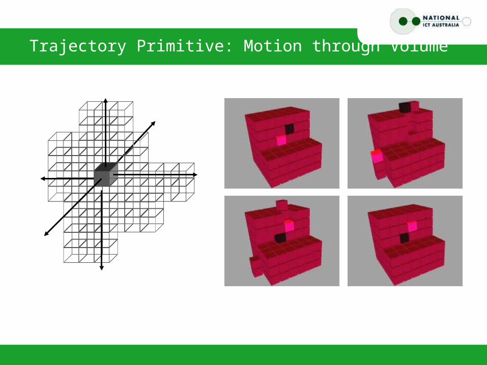
Trajectory Primitive: Motion through Volume

Reconfiguration with Tunneling

• TunnelSort• Uses limited

free-space• O(n2) in worst-

case (optimal)

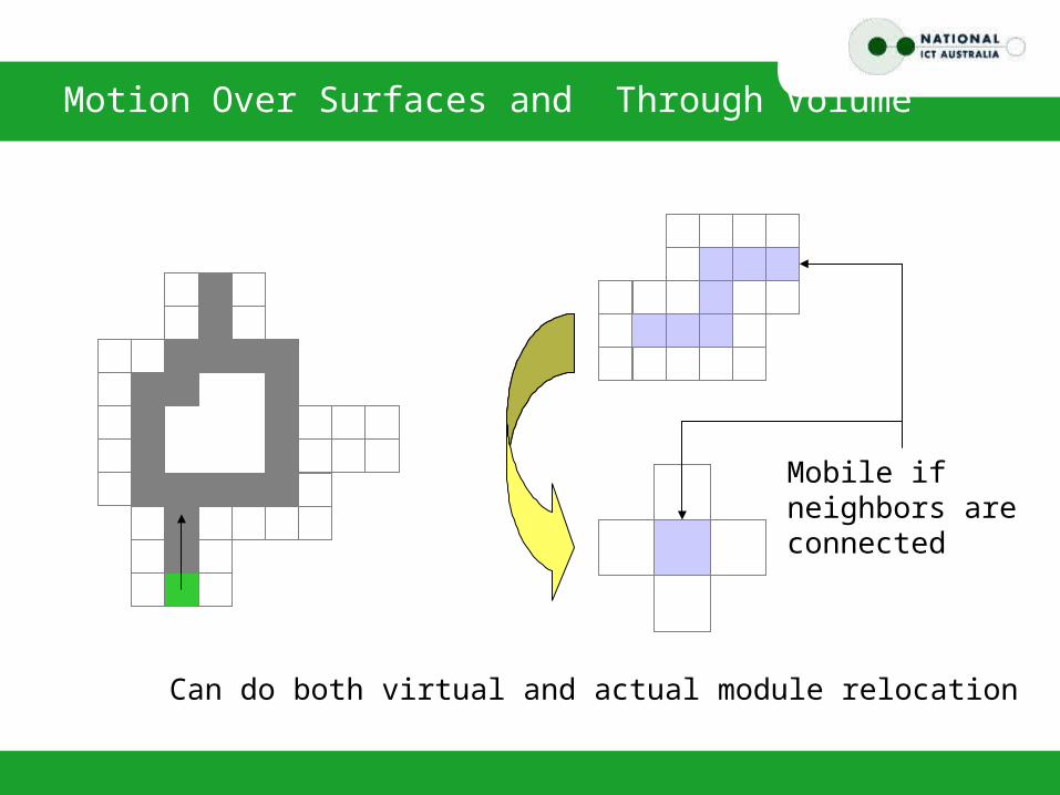
Motion Over Surfaces and Through Volume

Mobile if neighbors areconnected

Can do both virtual and actual module relocation

Reconfiguration Algorithm

• ConstrainedTunnelSort– Form goal shape

homogeneously– While not done

• Greedily choose modules to swap

• Swap using trajectory primitives

Only one move

possible – disconnect

ion!

No moves possible! 1 13 14

5 10 9 157 6 2 123 11 4 8

Maybe no solution!

Need to plan swap sequence!

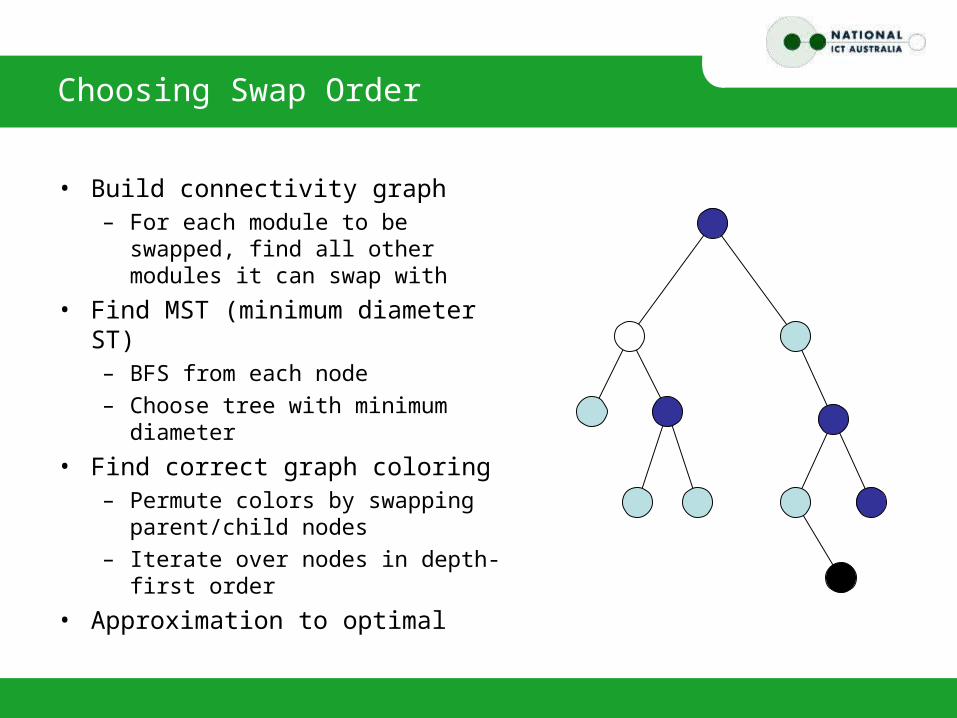
Choosing Swap Order

• Build connectivity graph– For each module to be swapped,

find all other modules it can swap with

• Find MST (minimum diameter ST)– BFS from each node– Choose tree with minimum

diameter

• Find correct graph coloring– Permute colors by swapping

parent/child nodes– Iterate over nodes in depth-first

order

• Approximation to optimal

Algorithm: Constrained TunnelSort

Homogeneous phase

• While not done– Choose module m

and position p, where m needs to move and p needs to be filled

– Find tunnel path from m to p

– Use virtual module relocation to move m along path

Heterogeneous phase

• Build connectivity graph of swappable modules

• Search for feasible swap sequence using MST-based algorithm

• Execute swaps using tunneling

O(n)

O(n)

O(n)

O(n)

O(n2

)

O(n2

)

O(n2

)

O(n2

)

O(n4

)

O(n2

)

O(n)

O(n)

O(n2

)

Example

Example

Outline

• Introduction• Reconfiguration, no obstacles

– Motion over surface– Motion through volume

• Algorithm: ConstrainedTunnelSort– Motion both over surface and through volume– Planned swap sequence– Complexity analysis

• Discussion

Discussion

• Algorithmic results– Solves heterogeneous reconfiguration among obstacles– Worst-case is uncommon in practice (m = t = p = n)– Average-case quadratic with more realistic estimates of

m,t,p.– Both centralized and decentralized versions

• Compliant locomotion– Series of goal configurations specified as overlapping

bounding boxes

• Position constraints

Position Constraints

• Objective– Maintain relative position

of single module during reconfiguration

• Assumptions– Non-exact goal

configuration representation

• Results– Initial solution

Next Steps

• Decrease number of moves, increase computation– Approximation of optimal path length

• Goal configuration determination– Alternative goal specifications (bounding box, etc.)– Use learning

Acknowledgements

• This talk describes work performed in the Dartmouth Robotics Laboratory. Support for this work was provided through NSF CAREER award IRI-9624286 and NSF awards IRI-9714332, EIA-9901589, IIS-9818299, and IIS-9912193, and a NASA SpaceGrant award. We are very grateful.

• Portions of this work were performed at National ICT Australia (NICTA). NICTA is funded by the Australian Government's Department of Communications, Information Technology and the Arts and the Australian Research Council through Backing Australia's Ability and the ICT Centre of Excellence program.