Reconciling competing models: a case study of wine fermentation

kinetics

Rodrigo AssarINRIA Bordeaux project-team MAGNOMEjoint with Université Bordeaux and CNRS

Rodrigo.Assar@inria.frFelipe A. Vargas, David J. Sherman

ANB 2010: RISC, Castle of Hagenberg, Austria, July 31-August 2

Wine fermentation

Need : more general model that better adapts to different conditions

Need : general method for this kind of reconciliation

Talk StructureIntroduction

Motivation and GoalMethods

System Analyzed models Steps of the approach

Results

Statistical results Constructive step Analysis

Summary and Perspectives

Introduction: Motivation

Wine industry: 5 mill. of tonnes/ year in France

Losses from fermentation problems (stuck and

sluggish): 7 billion of euros/year

Many different models to explain the wine

fermentation process

Not good results on not training data

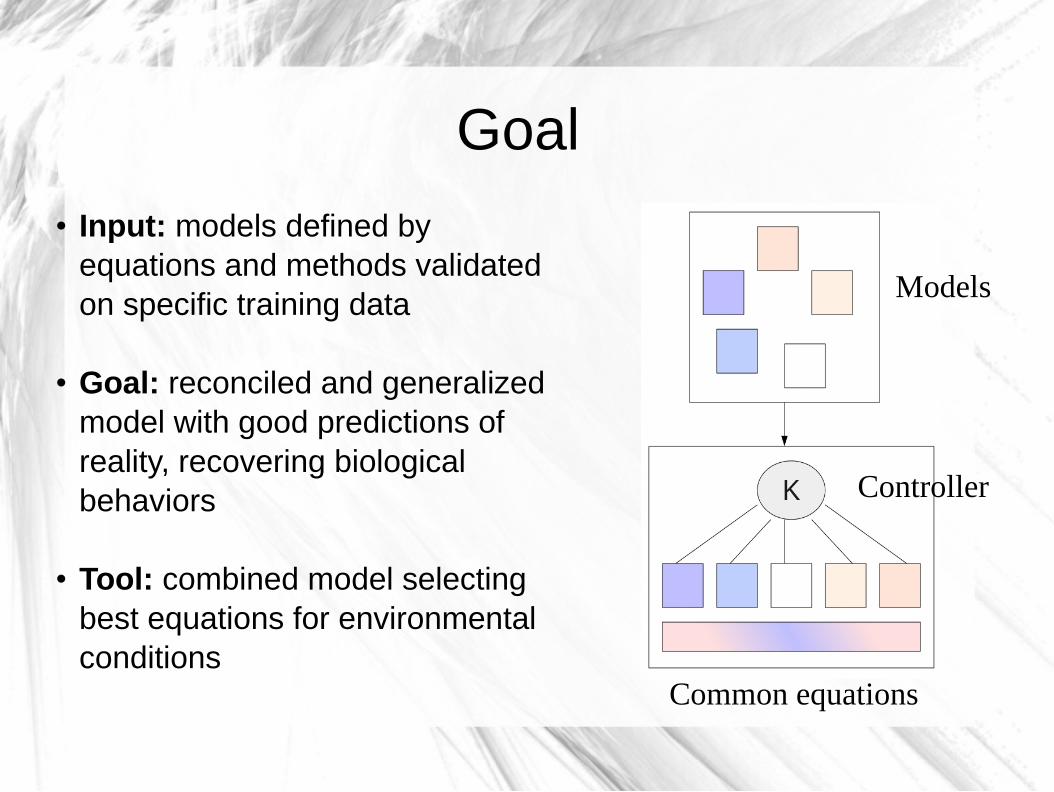
Goal Input: models defined by

equations and methods validated on specific training data

Goal: reconciled and generalized model with good predictions of reality, recovering biological behaviors

Tool: combined model selecting best equations for environmental conditions

Models

Controller

Common equations

SystemAgent: yeast

Resources: sugar and nitrogen

Other environmental factors: nutrient, pH, yeast populations and flora

Product: alcohol

By-products: carbon dioxide gas, heat

Analyzed modelsColeman et al., 2007

Scaglia et al., 2009

Pizarro et al., 2007

feedback

Steps of our approach

• Symbolic step: obtaining homogenous form, separating linear and secondary effects

• Statistical step: classifying the simulation results according to adjustment of experimental results

• Constructive step: building the combined model

Identifying effects

Effects represented by coefficient equations:

μA, ε

A, σ

A: linear effect of X

A on X, EtOH and S rate.

μ(1), ε(1), σ(1): linear effect of X on X, EtOH and S.

εCO2

: linear effect of dCO2/dt on EtOH.

μ(2) and σ(2): quadratic effect of X on S.

Rewriting models

Coleman et al., 2007 Scaglia et al., 2009 Pizarro et al., 2007

μ(2) μ(1)

Experimental dataM M (50-240 mg/l)

L (160-240 g/l) H (240-551 mg/l) 1(0-19 °C) H M

(240-308 g/l) H 2 3

M M 1 1 1M H 1 1 6 1

(20-27 °C) H M 1H 1 2

M M 1 1 1H H 2 1 2

(28-35 °C) H MH 1

Temperature Sugar Nitrogen Biomass Ethanol Sugar

Pizarro et al., 2007 Malherbe et al., 2004 M-F et al., 2007

We identified configuration levels L: Low, M: Moderate, H: High Statistical information: data sets per configuration, standard deviationBiological information: fermentations of S. cerevisiae, different strains

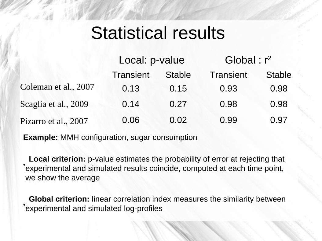
Statistical results

Pizarro et al., 2007

Coleman et al., 2007

Scaglia et al., 2009

Local: p-value Global : r2 Transient Stable Transient Stable

0.13 0.15 0.93 0.98

0.14 0.27 0.98 0.98

0.06 0.02 0.99 0.97

Example: MMH configuration, sugar consumption

Local criterion: p-value estimates the probability of error at rejecting that experimental and simulated results coincide, computed at each time point, we show the average

Global criterion: linear correlation index measures the similarity between experimental and simulated log-profiles

Statistical conclusions

There is no best model for all conditions

Quality depends on configuration of factors: level of temperature, sugar and nitrogen; temporal phase

For all the variables there exist models of good adjustment to experimental data

Combined model

Canonical representation

Factors-dependent coefficients

Initial condition-dependent equations

Configuration?Configuration?

HHHHHHMMM

Example: sugar uptake in MMH

Mendes-Ferreira data Pizarro data Coleman model Scaglia model Pizarro model Combined model

-- – x x x x x x xxxxxxxxx xxxxxxxxx xxxxxxxxx - - - - - - -

Initial conditions :20°C, 200 g/l of S, 267 mg/l of N

Summary• Combined model of wine fermentation kinetics

• Reconciling models steps:

• Symbolic: obtention of homogenous form. Polynomial for ODE systems

• Statistical: region-based analysis

• Constructive:

• Criterion to select best models• Combined model, coefficients depend of

factors levels: initial configuration and temporal phase

Perspectives Automatically homogenizing and combining of

models without revalidating

Automatically finding regions

Adding strain-specific effects

Considering competing populations

Acknowledgements

David J. Sherman

Pascal Durrens

Elisabeth Bon

Nicolás Loira

Natalia Golenetskaya

Anasua Sarkar

Aurelie Goulielmakis

Tiphaine Martin

Alice Garcia

Eduardo Agosin

Biotechnology Laboratory of Pontificia Universidad Católica de Chile

Jean-Marie Sablayrolles

Equipe de Microbiologie et Technologies des Fermentations, INRA

Thanks for Thanks for your your

attention!!attention!!!

Coleman Scaglia Pizarro

Temp. Sug. Nit. Biomass Ethanol Sugar Biomass Ethanol Sugar Biomass Ethanol Sugar

Trans. Stable Trans. Stable Trans. Stable Trans. Stable Trans. Stable Trans. Stable Trans. Stable Trans. Stable Trans. Stable

L M M

H

H M

H

M M M

H

H M

H

H M M

H

H M

H

Very good Good Little wrong Wrong

Very good:Very good: local and global criterion very favorable: p≥0.1 and corr≥0.98.

Good:Good: one criterion very favorable, other only favorable: 0.05≤p<0.1 or 0.95 ≤corr<0.98

Little wrong:Little wrong: one unfavorable (p< 0.05 or corr< 0.95) and other favorable or superior.

Wrong:Wrong: both criteria are unfavorable.

The limit cases: If local criterion is absolutely unfavorable (p= 0) we qualified in WrongWrong, if local criterion is unfavorable (but not absolutely) and global criterion is optimum (corr= 1) we considered it GoodGood.